Economics: an emerging small world?

Sanjeev Goyal∗ Marco van der Leij†

Jose Luis Moraga-Gonzalez‡

Preliminary version: November 2003This version: January 2004.

AbstractThis paper examines the small world hypothesis. The first part of the paper exam-ines the evolution of a particular world: the world of journal publishing economistsduring the period 1970-2000. We find that in the 1970’s the world of economics wasa collection of islands, with the largest island having about 15% of the population.Two decades later, in the 1990’s the world of economics was much more integrated,with the largest island covering close to half the population. At the same time, thedistance between individuals on the largest island had fallen significantly. Thus webelieve that economics is an an emerging small world.

What is it about the network structure that makes the world small? Our firstfinding is that the distribution of number of co-authors is very unequal (fat tails arepresent) and there are many stars (these are highly connected economists work witheconomists who have few or no other co-authors). Thus the world of economists is aset of inter-linked stars. Our second finding is that the increase in average numberof co-authors is the main explanation for the growth in the giant component as wellas the fall in average distances in it.

We take the view that individuals decide on whether to work alone or with others;this means that individual incentives should help us understand why the economicsworld has the structure it does. The second part of the paper develops a simpletheoretical model of co-authorship. The main finding of the model is that in thepresence of productivity differentials and a shortage of high productivity individuals,inter-connected stars will arise naturally in equilibrium. Falling costs of communi-cation and increasing credit for joint research lead to greater co-authorship and thisis consistent with the growth in the size of the giant component.

∗University of Essex and Tinbergen Institute. E-mail: sgoyal@essex.ac.uk†Tinbergen Institute, Erasmus University Rotterdam. E-mail: mvanderleij@few.eur.nl‡Erasmus University Rotterdam, Tinbergen Institute and CESifo. E-mail: moraga@few.eur.nl

We thank V. Bhaskar, Ken Burdett, Alberto Bisin, Francis Bloch, Alessandra Casella, Andrea Galeotti,Christian Ghiglino, Guillaume Haeringer, Alan Kirman, Otto Swank and participants at several seminarsfor useful comments.

1

1 Introduction

The idea of a small world is a very simple one. Tom and Sara are said to be at a distanceof 1 if they know each other and they are at a distance 2 if they do not know each otherbut have a mutual acquaintance and so on. The world is said to be small if the averagedistance between people is very small relative to the size of the population. The order ofnumbers in this claim is important: for instance, in a world of 5 billion people the averagedistance between people may well be around 6 (leading to the expression ‘six degrees ofseparation’). The idea that almost all people in the world are socially very close to eachother is a very intriguing one. It is also potentially a very important one as the structureof information flows and interaction between individuals has profound implications fora wide range of economic and social phenomena.1 In this paper we first examine theempirical content of the small world idea in the world of economists and then develop asimple individual incentives based model to help understand the factors that make theeconomics world small.

Our empirical work looks at the world of economists who publish in journals and weexamine the evolution of this world over a thirty year period, from 1970 to 2000. We splitthis period into three ten year intervals, 1970-1979, 1980-1989, and 1990-1999. For eachten year period we consider all papers published in journals listed by EconLit. This dataset contains a very large amount of information on a variety of variables. In this paperour interest is on three sorts of variables: the names of economists who have published atleast one paper in one of the journals in the list, whether these papers are co-authored orsingle authored and the journal where the paper was published. We use this informationto map a network of collaboration for each ten year period: every publishing author isa node in the network, and two nodes are linked if they have published a paper or moretogether in the period under study. Our interest is in the properties of this network ofcollaboration and the changes in these properties over time.

We start with an empirical examination of the question: is the world of economics smalland is this property stable over time. We identify three features of the network thattogether provide an answer to this question. The first feature is the growth of the network:we find that the world of economists has grown sharply in numbers and has more thandoubled in the period from 1970 to 2000. This finding is consistent with the growth inthe number of fields/specializations and in the corresponding set of field journals duringthis period and it leads us to expect that the world has probably become ‘larger’. The

1In recent years a vast literature has appeared on the role of interaction structures. A variety of termssuch as local interaction, network effects, peer group effects, have been used in this literature. See e.g.,Bala and Goyal (1998, 2001), Ellison and Fudenberg (1993) on social learning, Goyal (1996) and Morris(2000) on norms of coordination, Eshel, Samuelson and Shaked (1998) on norms of cooperation, Allen andGale (2000) on financial fragility of different inter-bank loan networks, Glaeser, Sacerdote and Scheinkman(1996) on local interaction and crime, Hagerstrand (1969) and Coleman (1966) on technological diffusion,Watkins (1991) on spread of norms in fertility and marriage and Young (1998) on spread of norms ondriving.

2

second finding is about the interconnectedness of the publishing world. In the 1970’s thelargest group of interconnected economists comprised only about 15% of the population,and there was a large number of small groups. In contrast, in the 1990’s there was onehuge group of interconnected economists with about 40% of the total population and allthe other groups had shrunk in size sharply. The numbers are worth mentioning here: inthe 1970’s the largest group of economists contained about 5,200 economists while in the1990’s the largest group contained more than 33,000 members. The third finding is aboutthe structure of this giant group of economists. We find that the average distance inthis giant group is small and has fallen significantly over time (despite the growth of thegroup), while the level of clustering remains high. We summarize these findings as follows:in the 1970’s the world of economics was a collection of islands. Two decades later, in the1990’s the world of economics was much more integrated. Hence, the economics world isan emerging small world.

What is it about the number and distribution of links in the network that makes thisworld small? The first finding is that the average number of co-authors is very low. Forinstance, in the 1990’s, the average number of co-authors was less than 2, while the totalnumber of authors was over 80000. The second finding is that the distribution is veryunequal; there exists a fat tail in the distribution, with a significant number of authorshaving a very large number of links. In the 1990’s the per capita number of collaboratorswas 1.672 while the maximally connected economist had more than 50 collaborators.Moreover, the clustering in the network in the 1990’s was .157 while the clustering forthe most connected economist was only .02. This shows that the most connected authorhad many more links than his cohorts and also that he had very low overlaps among theirco-authors as compared to the average person in the network. These numbers lead us touse the term ‘stars’ for the most connected economists. Our third finding is about therole of these well connected nodes in integrating the network. In the 1990’s over 40% ofthe nodes were in the giant component but a deletion of the 5% most connected nodesleaves less than 1% of the nodes in the giant component, thus completely destroying thenetwork.

We next examine the role of the different micro variables in explaining the main aggregatechanges noted above. We are specially interested in understanding the role of changes inaverage degree versus changes in link patterns. Our main finding is that the increase inaverage degree is the crucial factor in explaining the growth in the giant component andthe fall in average distances. This conclusion seems to contradict a widely held view thatthe world is becoming smaller because people are forming ‘distant’ links more often.2

The empirical findings are fascinating and we would like to develop a theory to account

2In particular, our finding appears to be in conflict with the conclusion of a recent paper by Rosenblatand Mobius (2003). These authors study a network of economists publishing in 8 economics journals andfocus on average distances within the giant component. They argue that it is the change in link patternsthat accounts for lower average distance between economists. We discuss the reasons for the differentfindings in detail after presenting our results in section 3 below.

3

for them. There is a large literature on the small world phenomenon in physics andmathematics. This work takes as a given that the world is small; our empirical work,however, shows that average distances and size of giant component in our network changegreatly over time. We therefore need a theoretical approach which can explain the stablearchitectural features of the network (the existence of stars, short average distance, andhigh clustering) as well as the changes in the network (such as growing giant component,falling average distance and increasing degree).3

In the second part of this paper we develop an incentives based model with the followingfeatures. Research papers contain ideas and involve routine work; the quality of a paperdepends on the quality of ideas contained in it. Individuals have ideas and can do rou-tine work; however, some people are better at generating high quality ideas than others.Institutions reward individuals on their research output; this reward specifies a thresholdlevel of output quality that is considered for evaluation and also specifies a certain creditto single authored work and co-authored work. There are costs to writing papers whichincrease in the number of papers written in a research area. Similarly there are costs tomeeting and working with others which are increasing in the number of co-authors andwhich are also sensitive to the (network) distance between the authors. Analysis of thismodel tells us that stars – which embody unequal distribution of links and links betweenwell connected and poorly connected players – arise naturally in a world with produc-tivity differentials and shortage of high productivity players. We show that equilibriumnetworks will contain inter-linked stars and hence will exhibit short average distances. Wealso study the role of two economic developments: a decline in costs of communicationand an increase in credit to co-authored papers. We find that they both lead to an in-crease in the number of collaborators and therefore an equilibrium network with a higherdegree, something which helps explain the growth in the size of the giant component.

In recent years there has been a virtual explosion of research in the field of networks. Webriefly discuss two related bodies of work in economics and in physics, respectively.4 Thetheory of network formation is a very active field of research in economics; recent workincludes Bala and Goyal (2000), Jackson and Wolinsky (1996), Kranton and Minehart(2001), among others. Dutta and Jackson (2003) is a collection of some of the mainpapers and Goyal (2003), Jackson (2003) and Van den Nouweland (2003) provide surveyson the developing field. The most distinctive aspect of this work is the use of individualincentives to derive predictions on network architectures. This work has been almostentirely theoretical and our paper’s contribution is to introduce the empirical study oflarge evolving networks in economics.

3We discuss the work in physics in detail in Section 5.4The idea of a ‘small world’ has a long history in sociology. Theoretical work on it was initiated in the

1960’s by Pool and Kochen (this work was published in 1978) and experimental work was initiated byMilgram (1967). Systematic empirical work on this subject has been hampered by the great difficultiesin collecting reliable data sets on large social networks. Theoretical work also seems to have progressedslowly. For an interesting general account of the developments in this field, see Watts (1999) and for acollection of theoretical papers until the late 1980’s, see Kochen (1989).

4

The empirical properties of large social and economic networks have been investigatedextensively by physicists in recent years; see e.g., Barabasi and Albert (1999), Barabasi,Albert and Jeong (1999), Newman (2001a,2001b,2001c, 2003) and Watts and Strogatz(1998). For comprehensive surveys of the work in physics see Albert and Barabasi (2002)and Dorogovtsev and Mendes (2002). This work focuses on the statistical properties oflarge networks, and uses a variety of techniques ranging from random graph theory tomean field analysis to elaborate on different features of observed networks. This workis discussed in detail in section 5. Here we briefly discuss two ways in which our papercontributes to this body of work. The first contribution is the incentives based approachwe develop. We believe that networks of scientific collaboration are an outcome of delib-erate decisions by individual economists. This means that the observed networks reflectthe technology of production of knowledge and the incentives faced by individuals. Weare thus interested in developing a model where technology and incentive schemes aremodelled explicitly and we can study their effects on collaboration networks systemati-cally. The second contribution of our paper is our empirical work; several aspects of it arenovel. To the best of our knowledge our paper is the first to study economics collaborationnetworks; existing work concerns the natural sciences, medical sciences and mathematics.This is interesting since these networks seem to exhibit different properties. For example,the relative size of the giant component and the number of co-authors seem to be verydifferent in economics as compared to physics or medical sciences. Moreover, we lookat the properties of the network over an extended period of time (thirty years) and thisallows us to study the impact of different technological and economic factors on the net-work, something which has not been done before since earlier studies have looked at thenetwork over relatively short periods of time (the maximum period of time covered seemsto be 8 years, see Albert and Barabasi (2002)). This difference in time horizon allows usto show the small world property is not a ‘constant’ of social networks; in particular, wefind that in the 1970’s the world of economics was fragmented into many groups and wasnot small, but that it is slowly getting integrated and is becoming a small world.

Our paper is also a contribution to the literature on different aspects of economics research;recent work includes Ellison (2002a, 2000b), Laband and Tollison (2000), among others.In particular, the increase in co-authorship has been noted and the reasons for it havebeen explored in Hudson (1996), while the role of substantial and increasing informalintellectual collaboration is explored in Laband and Tollison (2000). Hamermesh andOster (2002) present evidence which suggests that collaboration among distant authorshas increased over the years. A variety of arguments – such as increasing specializationand the falling costs of communication among others – have been proposed to explainincreasing co-authorship among economists.

The rest of this paper is organized as follows. Section 2 presents basic notation and defi-nitions. Section 3 contains our empirical analysis. Section 4 develops an incentives basedmodel to explain these network patterns while section 5 discusses alternative explanations.Section 6 contains concluding remarks.

5

2 Networks

We start by setting down some basic notation which is useful to discuss network featuresprecisely. Let N = {1, 2, .., n} be the set of nodes in a network. We shall refer to n asthe order of the network. We shall be looking at undirected links in this paper, and fortwo persons/nodes i, j ∈ N , we shall define gi,j ∈ {0, 1} as a link between them, withgi,j = 1 signifying a link and gi,j = 0 signifying the absence of a link. If two persons havepublished a paper together then they are said to have a link between them; if they havepublished no papers together then they have no link. Thus the information on authorsand papers allows us to construct a network of collaboration. We shall say that thereis a path between i and j either if gi,j = 1 or if there is a set of distinct intermediateco-authors j1, j2...jn, such that gi,j1 = gj1,j2 = ... = gjn,j = 1. The collection of all linkswill be denoted by g. The set of nodes and the links between them will be referred to asa network and denoted by G(n, g). We shall define Ni(G) = {j ∈ N : gi,j = 1}, as the setof people with whom i has a link in network G and ηi(G) = |Ni(G)|.

Two persons belong to the same component if and only if there exists a path betweenthem. The path relation therefore defines a partition of the network into components. Fora network G the partition will be denoted as P (G) = {C1, ..., Cm} with m ≥ 1. In casem = 1 we have a connected network and in case m = n we have the empty network. Thecomponents can be ordered in terms of their size, and we shall say that the network hasa giant component if the largest component fills a relatively large part of the graph andall other components are small, typically of order O(log n), where n is the total numberof vertices.

The geodesic distance between two nodes i and j in network G is the length of the shortestpath between them, and will be denoted by d(i, j; G). If there is no path between i andj in a network G then we shall set d(i, j; G) = ∞. In case G is connected, the averagedistance between nodes of a network G is given by

d(G) =

∑i∈N

∑j∈N d(i, j; G)

n(n− 1)

If G is not connected then the average distance is formally speaking infinite. In our datathe network is not connected and so to study distances we shall use the average distancein the giant component as a proxy for the average distance in the network. The maximumdistance between any pair of nodes in a network G is referred to as the diameter of thenetwork and it is given by

D(G) = maxi,j∈N

d(i, j; G)

Another measure of short distances, which is defined both for connected and unconnectednetworks, is the average size of the k-neighborhood. The k-neighborhood for an individuali is defined as

N ki (G) = {j ∈ N \ {i} : d(i, j; G) ≤ k}

6

while the size of i’s k-neighborhood is given by ψki (G) = |N k

i (G)|/(n− 1). Hence ψki (G)

is the fraction of people in the network who are at k or less degrees of separation fromindividual i. The average size of the k-neighborhood is then ψk(G) =

∑i ψ

ki (G)/n. This

statistic gives an estimate of the probability that two random nodes are connected withink degrees of separation.

The clustering coefficient of a network G is a measure of the correlation between links ofdifferent individuals. The level of clustering in an individual i’s neighborhood is given by

Ci(G) =

∑l∈Ni(G)

∑k∈Ni(G) gl,k

ηi(ηi − 1)

for all i ∈ N ′ ≡ {i ∈ N : ηi ≥ 2}, This ratio tells us what percentage of a person’sneighbors are neighbors of each other. The clustering coefficient for the network G can beobtained by averaging across all persons in a network. We shall use an averaging schemewhich weights different persons by the size of their neighborhood. This leads us to thefollowing definition for the clustering coefficient:

C(G) =

∑i∈N ′

∑l∈Ni

∑k∈Ni

gl,k∑i∈N ′ ηi(ηi − 1)

We will sometimes refer to ηi as the degree of node i. In case η1 = . . . = ηn = η wewill refer to η as the degree of the network. In general the degree is not constant acrossnodes/individuals and there will be inequality in the number of links across individuals.To measure this inequality we will compute Lorenz curves and Gini coefficients for thedegree distribution. Suppose the set of nodes S ⊂ N is ordered, such that i < j ifand only if ηi < ηj for i, j ∈ S, and denote ns = |S| as the number of nodes in S and

LS(h) =∑h

i=1 ηi as the number of links in possession of the h least linked nodes. Thenthe Lorenz curve for S is given by connecting the points

(h/ns, LS(h)/LS(ns)) ∈ [0, 1]2.

for h = 0, . . . , ns. The Lorenz curve measures the fraction of links that are in possessionof the x% least linked nodes. Note that perfect equality, that is a constant degree acrossnodes in S, implies that the Lorenz curve follows the 45 degree diagonal.

The Gini coefficient GS measures the area between the Lorenz curve and the 45 degreediagonal. That is

GS = 1− 1

ns

ns∑

h=1

LS(h) + LS(h− 1)

LS(ns).

An alternative way to write this is in terms of the relative mean difference:

GS =

∑ns

i=1

∑i−1j=1(ηi − ηj)

(ns − 1)LS(ns).

7

We note that the Gini coefficient equals 0 in case of perfect equality and 1 in case ofperfect inequality, that is when only one individual forms all the links in the network(an impossibility in graph with two-sided links). A higher value of the Gini coefficient isinterpreted as greater inequality in the degree distribution.

A star network is a network where one node, referred to as the center node, is linked toall other nodes in the graph while all these other nodes are only linked to the center node.In some networks, there is no single center of the network, but there are a small numberof extremely well connected nodes each of whose partners are almost solely connected tothem. We shall, somewhat informally, refer to these well connected nodes as ‘stars’.

3 Empirical Patterns

We study the world of economists who published in journals which are included in thelist of EconLit. We cover all journal papers that appear in a 10 year window and we lookat three such windows: 1970-1979, 1980-1989 and 1990-1999. The list of journal articlesincludes all papers in conference proceedings, as well as short papers and notes. We donot cover working papers and work published in books. The main reason for not coveringworking papers is that this can potentially lead us into double counting. The main reasonfor restricting attention to journal articles is that the EconLit database starts coveringbooks from the 1980’s only and this would sharply restrict the time frame of our study.Table 1 provides an overview of the coverage of our data. Tables 2 and 3 give us dataon the number of EconLit journals and the number of articles published in these journalsover this period. The number of journals has grown from 196 in 1970 to 687 in 1999 whilethe number of journal articles in EconLit has grown from 62,569 in the 1970’s to 156,454in the 1990’s. In Table 3 we can also derive that the number of pages per article hasincreased from 12.85 to 16.49 and that less and less papers have a single author. Thistrend was highlighted in Ellison (2002a).

The coverage of the Econlit data set is clearly partial and to check the robustness of ourfindings, we also consider an alternative set of data. We use the list of the TinbergenInstitute Amsterdam-Rotterdam (hereafter TI list) to do this. This list of journals isused by the Tinbergen Institute to assess the research output of faculty members at 3Dutch Universities (University of Amsterdam, Erasmus University Rotterdam and FreeUniversity Amsterdam). The Institute currently lists 133 journals in economics and re-lated fields (econometrics, accounting, marketing, and operations research), of which 113are covered by EconLit in 2000. The appendix presents the list of these journals andTable 2 shows the growth of this set over the 1970-2000 period. We observe that out ofthe 113 journals in 2000, only 46 were covered by EconLit in 1970! While some of the newjournals are general interest journals, it is fair to say that most of the increase comes fromthe expansion in the number of field journals. We interpret this as evidence of a broad-ening as well as a deepening in the subject matter that is covered by economics. Table 4shows summary statistics for the TI list data set. Not surprisingly we see an increase

8

in the number of papers, the number of pages per paper and the number of coauthoredpapers.

We thus have six data sets: 3 for the set of all journals covered in Econlit and 3 for theset of TI journals, and we construct a network for each data set. We first find the nodesin the network by extracting the different author names that appear in the data. As inNewman (2001c) we distinguish different authors by their last name and the initials of alltheir first names. Consequently, authors with the same last name and different initials areconsidered different nodes. We note that a single author may sometimes be representedby two nodes because of misspellings in the data or because of non-consistent use of firstor last names. Further, for papers with more than three authors EconLit reports onlythe first author and the extension et alia. Therefore we do not consider articles with fouror more authors when constructing the co-authorship network. We then construct thewhole co-authorship network by adding links between those authors that have coauthoreda paper. We note that we do not weight the links, that is, we do not distinguish betweenmore or less prolific relationships.5

3.1 Aggregate patterns

Our analysis of the collaboration network starts with an examination of the order of thenetwork, i.e., the number of publishing economists. Table 5 tells us that the professionhas grown substantially in this period: the number of authors has grown from 33,770 inthe 1970’s to 81,217 in the 1990’s. In Table 3 we saw that the the number of publishedpapers has grown from 62,569 in the 1970’s to 156,454 in the 1990’s. Thus the numberof papers grew by almost 150% over the 30 year period, while the growth in the numberof authors is a little lower. This difference is reflected in a slight increase in the percapita number of articles from 2.35 in the 1970’s to 2.83 in the 1990’s. The data basedon the TI list in Tables 4 and 6 is consistent with this trend: the number of authors hasincreased from 14,051 in the 1970’s to 28,736 in the 1990’s, the total number of papershas increased from 26,802 in the 1970’s to 52,469 in the 1990’s, and so the per capitanumber of papers has increased slightly from 2.45 in the 1970’s to 2.85 in the 1990’s. Ourfirst finding is therefore the following: the number of journal publishing economists hasgrown substantially – more than doubling – over the period 1970 to 2000.

Thus the number of nodes of the network has increased significantly. What about thepatterns of connections between these nodes? We shall focus on four macroscopic statisticsrelating to the pattern of connections: the existence and size of a giant component, theaverage distance between the nodes in the giant component, the average size of the 10-neighborhood and the clustering coefficient in the giant component as well as in thenetwork as a whole.

5We also analyzed weighted networks, see Newman (2001c). Results are only slightly different. Wealso considered networks in which separate authors are distinguished by their last name and the firstinitial only. The conclusions are not affected by this extraction rule.

9

We start with a discussion on the existence of a giant component. Table 5 presents thesestatistics for the periods under study. In the 1970’s the largest component contained5,253 nodes which constituted about 15.6% of the population. This largest componenthas expanded substantially over time and in the 1990’s it contains 33,027 nodes which isroughly 40% of all nodes. Correspondingly, there has been a sharp fall in the proportionof isolated nodes from almost 50% in the 1970’s to about 30% in the 1990’s. At the sametime the second largest component has also declined in size: it had 122 members in the1970’s and only 30 members in the 1990’s. This trend is consistent with evidence in thedata on the TI list. Table 6 shows that the number of persons in the giant componenthas increased from 2,775 in the 1970’s to 14,368 in the 1990’s. In the 1970’s the giantcomponent constituted about approximately 20% of the total population, while in the1990’s it comprises 50% of the total population of economists. The proportion of isolatedauthors has declined from about 42% in the 1970’s to about 21% in the 1990’s. Finallywe note that here too the size of the the second largest component has declined sharplyfrom 74 to 31. These observations lead to our next finding: The largest component in thecollaboration network has grown substantially in absolute numbers as well as in relativesize while the size of the second largest component has declined sharply in absolute size.Moreover, the proportion of non-collaborating economists has declined sharply.

We now turn to the distance between the nodes in the network. As is the norm we setthe distance between nodes in the different components to infinity and we use the averagedistance between nodes in the giant component as a proxy for our measure of averagedistance in the network. We find that this average distance has declined from 12.86 inthe 1970’s to 9.47 in the 1990’s. We also note that this fall in average distance has beenaccompanied with a significant fall in the standard deviation in the distances betweennodes from 4.03 in the 1970’s to 2.23 in the 1990’s. This trend is consistent with thetrends observed in the data on journals in the TI list: Table 6 tells us that the averagedistance in the giant component has declined from 11.99 in the 1970’s to 9.69 in the 1990’swhile the standard deviation has declined from 4.02 in the 1970’s to 2.35 in the 1990’s.This leads to our next finding: The giant component has grown substantially in numbersbut at the same time it has become significantly smaller in terms of distances.

The above findings suggest that nowadays it is more likely that there exists a path betweentwo random economists and that on average this path is much shorter than it was in the1970s. This is also confirmed by the trend in the average size of the k-neighborhood.Tables 5 and 6 show that the size of 10-neighborhood has increased sharply – from .7%to 11.8% for the full EconLit data set and from 1.5% to 16.5% for the data set based onthe TI list of journals. This trend is also clear if we look at the size of 10-neighborhoodwithin the giant component. For the set of all journals, we find that the mean size of the10-neighborhood increased from 28.8% in the 1970’s to 71.2% in the 1990’s and a similarpattern arises for the TI list. Hence the probability that there are less than 10 degrees ofseparation between two random nodes has increased sharply.

We turn next to the level of overlap between co-authorship which is measured by the

10

clustering coefficient in the network. Table 5 shows that clustering coefficient for thenetwork as a whole was .193 in the 1970’s, .182 in the 1980’s and .157 in the 1990’s.Table 6 shows the clustering coefficients for the journals in the TI list. These observationslead us to our next finding: the clustering coefficient for the whole network is high in the1970-2000 period.6

The discussion on the data allows us to make three general points about the aggregatecharacteristics of the network of collaboration among economists during the period 1970-2000: the first point is about the number of nodes of the network: they have more thandoubled in this period. The second point is that distinct groups of co-authors seem tohave formed links with each other and this has led to the emergence of a giant group ofinterlinked economists which now covers about half of the total population. The thirdpoint is about the structure of this giant component: the average distance in this giantgroup has steadily been falling over time while the level of clustering has remained high.Taken together, these three remarks suggest that the world of economists is expandingbut at the same time becoming a small world where most of economists find themselvesjust a few degrees of separation away from any other economist.

3.2 Link patterns

What are the mechanisms underlying the emergence of the small world? Our approachto this question is founded on the idea that individual economists have a choice betweenwriting papers by themselves or in collaboration with others, and that the network ofcollaboration we observe arises out of the decisions they make in this regard. Individualdecisions on research strategies will thus depend on a variety of factors such as the costs ofdoing individual and joint work and relative rewards of alternative modes of research. It isalso likely that differences in individual productivity have a bearing on collaboration. Wewould like to develop a model of co-authorship in which these costs and the reward schemesare exogenous parameters while the link decisions and the networks of collaboration areequilibrium outcomes. Thus the crucial micro level data in this approach are the numberof collaboration links that an individual forms and the patterns of linking across othereconomists. We look next at these micro statistics in the data that we have assembled.

We start with the average number of links per capita. In all the data we have assembledwe observe the following trend: the average number of links/collaborators per capita hasgrown significantly in the period 1970 to 2000. For the set of all journals in EconLit, Ta-ble 5 tells us that there is almost a doubling in the per capita number of links/collaboratorsfrom .894 in the 1970’s to 1.672 in the 1990’s in the giant group. This figure covers allpublishing economists and it is useful to also examine the per capita number of collabora-tors among people who are in the giant component. Table 5 shows us that the per capita

6When we say ’high’ we mean that it is substantially higher than the clustering coefficient of a randomnetwork. For a discussion on this issue, see Section 5.

11

number of collaborators increased from 2.48 in the 1970’s to 3.06 in the 1990’s. This trendis also visible and clear cut in the TI list of Journals. Table 6 tells us that mean number oflinks has increased from 1.058 in the 1970’s to 1.896 in the 1990’s. Similarly, we find thatthe mean links per author has increased in this data set if we restrict attention to authorsin the giant component. This trend of increasing number of collaborators is related tothe trend in the proportion of co-authored papers. Table 3 shows that 25% of all articlesin EconLit were coauthored in the 1970’s, while 42% of the articles were coauthored inthe 1990’s. When we consider the TI list only, then the proportion of coauthored papershas increased from 28% in the 1970’s to 50% in the 1990’s (see Table 4). This trend ofincreasing collaboration is a well-known fact in the research literature, see e.g. McDowelland Melvin (1983) and Eisenhauer (1997).

Although the average number of collaborators per author has increased over time, theabove aggregate statistics do not provide information on whether this increase has beenequally distributed in the population of economists. We explore this issue by examiningthe distribution of links in the collaboration network more closely. Figure 1 shows thePareto plot for distribution of links: this plot shows on a log-log scale the degree of linksper author k on the x-axis and the tail distribution, i.e., the fraction of authors for whichηi ≥ k, on the y-axis. This graph shows that there is a first-order stochastic dominancerelationship over time. The distribution for the 1980’s first order stochastically dominatesthe distribution of the 1970’s, while the 1990’s degree distribution first order stochasticallydominates the degree distribution of the 1980’s. This yields us our first finding on themicro statistics of the network: the number of collaborators has been increasing consistentlythrough the 1970-2000 period for all quantiles.

Another remarkable aspect of Figure 1 is that the Pareto plot seems to converge to astraight line for high degree k. This suggests that at high quantiles the distributionconverges to a Pareto or power-law distribution.7 An important characteristic of sucha distribution is the existence of a fat tail. Indeed, extreme degree values appear morefrequently in the real data than in a binomial distribution fitted on the 1990’s data set.While under the fitted binomial distribution it is unlikely that any author has more than10 links, in reality we see that more than 1% of the authors have more than 10 links andsome of them have 40 to 50 links.

We explore the inequality in the number of links per author further by looking at Lorenzcurves and Gini coefficients. Figure 2 shows Lorenz curves in the 1970’s, 1980’s and 1990’sbased on the data set that includes all EconLit journals. We see an striking inequality inthe distribution of links: the 20% most-linked authors account for about 60% of all thelinks. The plot also reveals a decreasing trend in inequality over time. This observation isconfirmed by the Gini coefficients reported in Table 7. This trend is mainly explained by adecrease in the number of isolated authors — from 50% in the 1970’s to 30% in the 1990’s— since it implies that more and more authors are involved in co-authoring. Interestingly,

7A power-law distribution would take the form f(k) = αk−β , with α > 0 and β > 0.

12

if we adjust for this participation effect by ignoring isolated authors or by considering thegiant component only, then Table 7 shows that the trend is reversed. The above resultslead to the following finding: The distribution of links in the population is very unequaland exhibits a fat tail. Further, inequality in the number of links has increased withincomponents and it has decreased when we consider the whole network.

We now examine more closely the role of the individuals who are very well connected inthe network of collaboration. Table 8 tells us that in the 1970’s the maximally connectedperson had 25 links and the 100 most linked persons had on average 12 links. Lookingmore closely at the most connected individual we see three very striking features: one, thisperson published 44 papers out of which 42 (i.e., 95% of them) were co-authored; two, hehad 25 collaborators while the average number of collaborations per capita was less than1; and three, the clustering coefficient for this person was only .05, which is much smallerthan .193, the clustering coefficient of the network at large. Similarly, in the 1990’s themost connected individual published 66 papers, of which 64 were co-authored (this is97% of the total), had 54 collaborators (while the per capita number of collaborators wasunder 2) and a clustering coefficient of .02 (while the clustering coefficient of the networkas a whole was .157). Thus the most connected individuals collaborated extensivelyand most of their co-authors did not collaborate with each other. The most connectedindividuals can be viewed as ‘stars’ from the perspective of the network architecture. Acloser inspection of Table 8 reveals that these three patterns are quite general and hold forthe average of the 100 most linked individuals in the 1970’s, 1980’s and 1990’s. Table 8also tells us that the average number of links among the top 100 stars has more thandoubled, while clustering around the stars has decreased. This leads us to state: Thereis a large number of ‘stars’ in the world of economics and they co-author most of theirresearch output and the number of stars in the world of economics is increasing.

We next examine the role of the stars in connecting different parts of the network. Forthis purpose we compared the consequences of randomly deleting 2% or 5% of the nodeson network connectivity and clustering with the consequences of deleting star nodes. Wedo this for the network based on all EconLit journals. Table 9 shows the results. Wecan see that a removal of 5% of the authors at random has almost no effect on thenetwork connectivity and clustering. For the 1990’s, we find that the size of the giantcomponent goes down from .407 to .389, while the average distance within the giantcomponent increases marginally from 9.47 to 9.68. The effects on size of 10-neighborhoodand clustering co-efficient are similarly insignificant. By contrast, a removal of the 2%most connected nodes has a devastating effect on the network. The giant componentbreaks down and its share of the total network goes down from .407 to .256, while theaverage distance within the giant component increases from 9.47 to 19.00. The effectson the size of the 10-neighborhood are substantial. We would like to note also that theimpact on clustering coefficient is very substantial: it increases from 0.157 to 0.250 withthe removal of the 2% most connected individuals and to .344 on the removal of the5% most connected ones. These observations yield our finding on error tolerance of the

13

economics network : The stars play the role of connectors and sharply reduce distancebetween different highly clustered parts of the world of economics.

We would like to plot the networks for the periods of 1970’s, 1980’s and 1990’s to getan overall picture of the networks. This has proved to be very difficult due to the largenumbers of nodes involved. We have therefore tried to plot the local network aroundsome prominent well connected economists (Figures 3-6). These plots are fascinating andsuggest a number of ideas; we would like to draw attention in particular to one strikingfeature of the networks: hierarchy. For instance, in the plot for Joseph Stiglitz (Figure 3)we find that he is linked to several persons who are themselves ‘stars’ in the sense discussedabove. Furthermore, we observe that these star co-authors of Mr. Stiglitz typically donot work with each other and also that the co-authors of these persons typically do notwork with each other either. In particular, the co-authors of the stars do not work withMr. Stiglitz. Thus there seems to be a hierarchy of well connected persons. We find thisstructure remarkable as this hierarchy is mostly self-organizing. A similar structure canbe discerned in the plot for Jean Tirole (see Figure 4).

3.3 Explaining the emerging small world

There are two principal macro level changes in the structure of the economics network:one, the growth in giant component, and two, a fall in average distance within the expand-ing giant component. We now examine the relative importance of different micro-levelvariables – in particular the average degree – in explaining these macro level changes.

We start by noting that the number of nodes in the network has also changed over theperiod under consideration. Thus to understand the role of changes in average degreeand pattern of links we first need to control for changes in the number of nodes. We dothis in the following way: we delete nodes at random from the networks in the 1990’sand 1980’s to bring the number of nodes down to the level of nodes in the 1970’s. Thisprocedure results in an adjusted network for the 1980’s and 1990’s, respectively. Table 10summarizes our findings for the network based on the TI list journals.

We note that the average degree in these adjusted networks is quite comparable to theaverage degree in the actual network of the 1970’s. Thus we now have three networks–the adjusted 1990’s network, the adjusted 1980’s network and the actual 1970’s network– that have an equal number of nodes and similar average degree. Hence, any differencesin the aggregate properties of the network must be due to changes in the patterns of links.Our first observation is that the giant component comprised 17.3% of the population in1990’s adjusted network, 21.3% in the 1980’s adjusted network, and 19.7% in the 1970’sactual network: the size of the giant component is comparable in the three networks understudy. Our second observation is that the average distance was 14.79 in the 1990’s adjustednetwork, 13.74 in the 1980’s adjusted network, and 11.99 in the 1970’s actual network:the average distance is significantly higher in the adjusted networks as compared to the

14

actual 1970’s network. These observation and our earlier comments imply that changesin the patterns of links cannot account for the growth of the giant component or thefall in average distances within the giant component. Our experiment thus leads to theconclusion that the two aggregate trends we observe must be caused by the increase in theaverage degree over time.

In a recent paper, Rosenblat and Mobius (2003) argue that it is the change in patternsof links that explains the fall in average distances. Our finding seems to contradict thisargument. We would like to examine in detail the approach used by them to understandthe reasons for the conflicting conclusions.

We note that their analysis takes as a given the size of the giant component in the periodunder consideration. By contrast, the main finding of our empirical analysis is that thesize of the giant component has grown substantially over time. Indeed, this trend is robustand is to be observed in all the different collaboration networks we have studied. Thusthe scope of the analysis in the two papers is different. We will now explain how thisdifference in scope also matters in developing an explanation for falling distances withinthe giant component.

Rosenblat and Mobius (2003) look at a network of collaboration of authors who publishedin 8 core economics journals.8 They compare the collaboration network of 1975-1989 tothe network of 1985-1999 and the network of 1970-1989 to the network of 1980-1999.They consider the giant component only, and they observe that average degree in thegiant component has increased from 2.52 to 2.67 across the two networks. They controlfor this average degree by deleting links according to the ratio 1−C1/C2, where C1 is theaverage degree in the giant component between 1975-1989 and C2 is the average degreein the giant component between 1985-1999. They find that average distances are lowerin the giant component of the adjusted 1985-1999 network as compared to the actual1975-1989 network. This leads them to argue that it is changes in the pattern of linksthat has led to a fall in average distances in the giant component (see Table 6 in theirpaper).

We replicated their experiment and our results are reported in Tables 12 and 11 (seecolumns 1-3).9 Our first observation is that the average distance in the giant componentis different as compared to the figures they obtained. Our second observation is that the

8These journals are American Economic Review, Quarterly Journal of Economics, Journal of PoliticalEconomy, Econometrica, Review of Economic Studies, Review of Economics and Statistics, Rand Journalof Economics, and Brookings Papers on Economic Activity.

9We use a data set with the same 8 journals as Rosenblat and Mobius (2003). However, the datasets are not identical, as we have no information on the way the data issues mentioned in Section 3 aretreated in the analysis of Rosenblat and Mobius. We treat the data issues in the 8 journal data set asfollows; we ignore all papers with 4 or more authors and we distinguish authors by their last name andtheir initials. In Table 12 we consider all given name initials, while in Table 11 we only consider thefirst initial. Further, we included the Bell Journal of Economics in the data set being the ancestor of theRAND Journal of Economics.

15

average distance in the adjusted giant component is lower than the average distance in thegiant component of the actual 1975-1989 network. This is consistent with their finding.We now examine the connection between average degree and average distance.

A closer inspection of the Table 12 reveals that their method yields a giant componentin which the average degree is 2.60, which is significantly higher than 2.52 the averagedegree in the actual 1975-1989 network. Thus their control on average degree is notproperly implemented. The reason for this discrepancy is as follows: implementing theirprocedure involves deleting links at random, which in a large enough network shouldyield the same average degree in the adjusted network as in the actual 1970’s network.However, as links are deleted at random it is more likely that the authors with fewer linksare disconnected from the giant component. As a result, the average degree of authorsin the giant component of the adjusted network is higher than what was aimed for. Thiscan be seen in column 3 of Tables 12 and 11.

Our goal is to understand the relative role of changes in degree and pattern of links andso we would like to implement their procedure in a way that yields us a network withcomparable average degree and size of giant component. The simplest way to do this isto delete links of all agents and not just the links of authors in the giant component witha view to obtaining a network in which the overall average degree is equal to the averagedegree in the 1975-1989 network. This way of implementing the procedure also has thegreat merit of taking into account the changes in the size of the giant component overtime in a natural way. This is important because as we have already noted the size of thegiant component is changing substantially over time.

We have carried out this experiment, and our findings are reported in the last column ofTables 12 and 11. We now find that the results are quite different: the average distance inthe adjusted network is 10.59, while the average distance in the actual 1975-1989 networkis 10.39 implying that the average distance in the giant component of the adjusted networkis now actually larger than the average distance in the actual 1975-1989 network! A similarpattern obtains in the 20 year networks as well. We therefore conclude that changes invariables other than average degree do not lead to a decrease in average distances in thegiant component.10

10We note that in our experiment, the average degree in the giant component of the adjusted networkis 2.44 which is lower than the average degree of the giant component in the actual 1975-1989 network.This may create the impression that it is differences in the average degree in the giant component thatlies behind our finding. Our experiments with the networks based on the TI list show that this is notthe case. The average degree in the adjusted 1980’s network is 2.44 which is similar to 2.48 the averagedegree of the actual 1970’s network. However, the average distance in the adjusted 1980’s network is13.74 which is significantly larger than 11.99, the average distance in the giant component of the actual1970’s network (see Table 10).

16

3.4 Data robustness

We now briefly discuss some aspects of the data that we use. A shortcoming of the abovedata for our purposes is the partial coverage of the EconLit list. We observe that thislist has been growing over time and the data discussed above relate to this expandingworld. This pattern creates the following possibility: in the 1970’s the world of journalswas actually very similar to the one we observe today but the EconLit data set does notcapture this as it covered a small subset of journals and therefore excluded a large partof the journal publishing world. If this were true then the data above would be aboutthe world of EconLit authors but would not be a good indicator of the world of journalpublishing economists per se.

There are different ways of getting around this problem. We have already done onerobustness check by looking at the TI list of journals. We now carry out another robustnesscheck. We study the network of collaboration using only the subset of journals that appearin Econlit for the entire sample period. This is the route taken in Tables 14 and 16. Thenumber of authors has gone up significantly from 22,960 in the 1970’s to 32,773 in the1990’s, about 43%. We now turn to the statistics on the pattern of connections. Wenote that the largest component has grown from 3,076 nodes in the 1970’s, which wasabout 13% of all nodes, to 10,054 nodes in the 1990’s, which is about 30% of all nodes.Likewise, the percentage of isolated authors has fallen from about 50% in the 1970’s toabout 32% in the 1990’s. Thus the order of the network is increasing while the networkis becoming more integrated. This is also witnessed by the increase in the average size ofthe 10-neighborhood, which has grown from .6% to 2.8%. We note however that there isno trend in average distances in the giant component in the period under consideration.With regard to the micro statistics, Table 16 tells us that mean number of links per authorhas increased from 0.885 in the 1970’s to 1.386 in the 1990’s.

We finally consider a fixed set of five core journals, namely, American Economic Review,Econometrica, Journal of Political Economy, Quarterly Journal of Economics and Reviewof Economic Studies. Tables 13 and 15 show the results we obtain. The size of the giantcomponent has increased from 7% in the 1970’s to 25% in the 1990’s and the averagesize of the 10-neighborhood has increased from .5% in the 1970’s to 2.9% in the 1990’s.Further, the number of per capita collaborators has increased from .833 in the 1970’s to1.429 in the 1990’s and the clustering coefficient has remained high over time. Thereare some interesting differences though. First, we see no trend in distance. Second, thenumber of articles in the top 5 journals has decreased from 5,023 in the 1970’s to 3,705in the 1990’s. This appears to be mainly due to an increase in the length of the papers.We also observe a much more significant increase in the proportion of coauthored papers.This is highlighted in Figure 7. The figure shows the proportion of coauthored articlesfor different classes of journals classified on the basis of a quality criterion (AA (top 5journals), A (second tier) and B (third tier)) as used by the Tinbergen Institute (see theappendix for the list of journals and its classification as AA, A, or B journals). We see

17

that in the 1970’s these 5 journals had the smallest fraction of coauthored papers, whilein the 1990’s they have the highest proportion of co-authored papers.

The observations lead us to conclude that there is a significant increase in the size of thegiant component as well as in the average degree of the network, but there appears to beno general trend in the average distances in the giant component in these two networks.

3.5 Economics and other subjects

We would like to compare the collaboration network in economics with the networks inother subjects. Table 17 presents a summary of statistics for economics along with thosefor physics, medical sciences, computer science and mathematics. There are significantdifferences in period covered and the status of the publications so this table should beseen as being suggestive only. First, we would like to draw attention to the substantialdifferences in the size of the giant component. We observe that both in physics as wellas in medical sciences, the giant component covers almost the whole population, while ineconomics, computer science and mathematics the giant component covers around one halfof the population only. Second, we would like to mention the average distances: here againwe find that average distances in physics and medical sciences are very small as comparedto the average distances observed in economics, computer science and mathematics. Thesedifferences appear to arise out of substantial differences in the overall number of personsin the network as well as the per capita number of links: in the medical sciences data setthe number of authors was over 2 million and the average number of links was 18.1 (for afive year period, 1995-1999), while in economics the total number of authors was 156,454while average number of links was only 1.67 (over a ten year period, 1990-1999).

4 An incentives based explanation

In this section we try to explain the observed patterns of co-authorship in terms of a modelof individual incentives. We are specially interested in explaining the following featuresof the co-author network: short average distances and high clustering and growth in sizeof giant component. Our model has three main aspects: productivity differences acrossindividuals, a technology of knowledge production, and academic reward schemes.11

4.1 Model

We suppose that there are n players and that a player can be either of High type or Lowtype. There are nh High-type players, and nl Low-type players, and n = nh + nl. We

11For a related model of co-authors, see Jackson and Wolinsky (1996). Their interest is in comple-mentarities in collaboration and their equilibrium networks are characterized by complete components ofdifferent sizes.

18

shall assume that 1 < nh << nl and that nl is sufficiently large. We shall denote theset of players by N . Players make decisions on their research strategy: whether to writealone or with others, and if with others, how many co-authorships to form and with whichtypes of players; they also decide how many papers to write and how much effort to putin each paper that they write.

Let gxij ∈ {0, 1} model i’s decision on whether to participate in a project x with author

j, where a value of 1 signifies participation while a value of 0 signifies non-participation.Let ex

ii denote the effort that player i spends on a single-authored paper x, and let exij,

refer to the time that he spends on a joint paper x with coauthor j. We assume that fora paper to be written the total effort put in by its authors must be at least 1. A researchstrategy of a player is then given by a row vector, si = {(gx

ij, exij)x∈{1,..,m},j∈N}, where m is

the number of projects that a player participates in either individually or with any othersingle coauthor.12 A player j is a coauthor of player i if gx

ij = gxji = 1 for some paper x.

Let ηi(s) be the number of coauthors of player i in research strategy s.

A paper consists of ideas and technical routine work. The quality of a paper dependsonly on the quality of the ideas it contains and the ideas of the paper in turn depend onthe type of the authors of the paper. A High-type author has high quality ideas, while aLow-type author has low quality ideas; the high and low quality types of ideas are denotedby th and tl, respectively, where th > tl > 1. It is natural to assume that a type i authorwill write single-authored papers of quality ti only, i = h, l; we assume that if two authorsi and j jointly work on a paper the quality of the paper is given by ti · tj. Thus qualityof a paper can be q ∈ {t2h, thtl, th, t2l , tl} = Q.

We now elaborate on the costs and benefits of writing papers alone and with others.We first note that writing a paper takes time and effort and this has costs in terms ofresources and the leisure sacrificed. We assume that the marginal costs of writing pa-pers increase with the number of papers, reflecting increasing marginal opportunity costsof time. Maintaining a coauthor relationship involves communication and coordinationacross different projects and possibly different partners and these costs are likely to in-crease as the number of co-authors increases. This leads us to assume that the marginalcost are increasing in the number of coauthors, ηi(s). Given these considerations, we areable to write down the costs of a research strategy si for a player i faced with a researchstrategy profile s−i, as

∑j∈N

c

∑

x∈{1,..,m}ex

ij

2

+ fηi(s)

2

2(1)

with f > 0. This cost specification captures the idea that a collaboration relation be-tween two individuals i and j is a research project and that the costs of coming up with

12The idea of m is introduced for notational convenience and is different from a capacity constraint.This will become clear when we model the costs of writing papers below.

19

interesting ideas and papers increase as more papers are written within the project. Thisleads us to suppose that writing m papers with m coauthors is less costly than writing mpapers with a single coauthor. This assumption pushes individuals toward diversificationof collaborators. On the other hand, our assumption that costs of linking with others areconvex in the number of links pushes toward fewer collaborators. The optimal number ofcollaborators trades off these two pressures and depends also on the rewards associatedwith scientific activity.

The rewards from publishing a paper depend on a variety of factors such as its qualityof papers and the number of coauthors. We shall suppose that a person is paid on thebasis of quality weighted index of papers he publishes, there is discounting of joint workand that there is a minimum quality requirement such that only papers above this qualityare accepted for publication. We shall suppose that this threshold is given by q whereq ∈ [1, t2h]. One interpretation of this threshold is in terms of different journals: a higherranked journal can be more choosy in the papers it publishes and so it will have a higherthreshold as compared to a lower ranked journal.

We suppose that a single-author paper of quality q gets a reward q, while a 2-author paperof quality q yields a reward rq to each author, where r ∈ (0, 1) reflects the discountingfor joint work in the market. Thus r = 0 means that joint work is given no credit, whiler = 1 means that each coauthor of a joint paper gets credit equal to the credit due to anauthor of a single author paper.13

For a strategy profile s, let Ixij(e) be an indicator function, which takes on value 1 if

gxij = gx

ji = 1, exij + ex

ji ≥ 1, and qxij ≥ q, and it takes a value of 0, otherwise. Given these

considerations, for a strategy si and faced with a strategy profile s−i, the payoffs to aplayer are as follows:

Πi(si, s−i) =∑

j 6=i

∑

x∈{1,..,m}Ixijrq

xij +

∑

x∈{1,..,m}Ixiiq

xii −

∑j∈N

c

∑

x∈{1,..,m}ex

ij

2

− fη(s)2

2. (2)

We study the architecture of networks that are strategically stable. Our notion of strategicstability is a refinement of Nash equilibrium. A strategy profile s∗ = {s∗1, s∗2, ..., s∗n} is saidto be a Nash equilibrium if Πi(s

∗i , s

∗−i) ≥ Πi(si, s

∗−i), for all si ∈ Si, and for all i ∈ N .

In our model a coauthoring decision requires that both players wish to participate in thepaper. It is then easy to see that an autarchic situation in which no one does any jointwork is always a Nash equilibrium. More generally, for any pair i and j, it is always amutual best response for the players not to participate in any joint projects. To avoidthis type of coordination problem we supplement the idea of Nash equilibrium with therequirement of pair-wise stability. An equilibrium network is said to be pair-wise stable

13We are assuming here that different types involved in a collaboration get the same reward; our resultsdo not change qualitatively if we assume that Low types get a lower payoff than High types.

20

if no pair of players has an incentive to initiate one or more new joint papers. We definepair-wise stable equilibrium as follows:

Definition 1 A strategy profile s∗ is a pair-wise stable equilibrium if the following con-ditions hold:

1. s∗ constitutes a Nash equilibrium.

2. For any pair of players, i and j there is no strategy pair (si, sj) such that Πi(si, sj, s∗−i−j) >

Πi(s∗i , s

∗j , s

∗−i−j) and Πj(si, sj, s

∗−i−j) > Πj(s

∗j , s

∗j , s

∗−i−j).

In what follows, for expositional simplicity we shall use the short form – pws-equilibrium– while referring to pair-wise stable equilibrium. This notion of equilibrium is taken fromGoyal and Joshi (2003). We shall say that a network is symmetric if all equal-type playershave the same number of links with each of the two types of players. This will allow usto talk of the typical number of collaborations between a typical i and j type of playersand use ηij to refer to this number.

4.2 Equilibrium analysis

We start characterizing equilibrium networks under the assumption that in a joint project,each author contributes one half of the time needed for routine work and gets credit r forthe joint paper. This may be interpreted as a model with no transfers. We note that theoptimal choice of number of papers is independent across pairwise collaboration ties. Thisis due to the cost specification which is additive across projects with different co-authorsand own projects. Our first result derives the optimal number of papers that High typeand Low type authors will write on their own and with others.14

Proposition 1 Suppose that threshold quality for publication is lower than tl. A High typeplayer optimally chooses m∗

h = th/2c single author papers, m∗hh = 2rt2h/c papers in a HH

collaboration, and m∗hl = 2rthtl/c papers in HL collaboration. A Low type player optimally

chooses m∗l = tl/2c single author papers, m∗

lh = 2rthtl/c papers in a LH collaboration, andm∗

ll = 2rt2l /c papers in LL collaboration.

Proof: For a High type the optimization problem with respect to single author papers is

maxmh

thmh − cm2h (3)

Straightforward calculations yield m∗h = th/2c. Similarly, for a High type the optimal

number of papers in an HH collaboration is the solution to the following optimizationproblem:

maxmhh

rt2hmhh − c[mhh

2

]2

(4)

14In what follows we treat the number of papers and the number of co-authors as continuous variables.

21

This optimization problem yields us the solution that m∗hh = 2rt2h/c. Similarly, the optimal

number if papers for a H type in a HL collaboration are given by m∗hl = 2rthtl/c.

Given that the publication threshold is below tl, L types will also write papers on theirown. It follows from above calculations for the H-type players that the optimal numberof single author papers for an L-type are m∗

l = tl/2c. Using arguments analogous to theabove we can also conclude that the optimal number of papers for the Low type in a LHcollaboration is m∗

lh = 2rtlth/c, while the optimal number of papers in a LL collaborationis m∗

ll = 2rt2l /c.¥

This proposition tells us that H-types will write more single authored paper than L-types. Moreover, the optimal number of papers in a HH relationship is greater than thenumber of papers in a LL co-author relation. These results follow directly from the initialproductivity differences across players. We also note that the number of optimal papersvaries negatively with the costs of writing papers, while they vary positively with theindividual credit given in co-authored papers.

One implication of the above result is that different type of players get very differentaggregate returns from working alone and working with others. Moreover, players ofdifferent types also get very different payoffs from co-authorship relations. Let πi refer tothe payoff that a i type player gets from working alone, and πij refer to the reward that atype i player gets from working with a type j player. Then the above proposition allowsus to write down the following payoffs for different type players.

π∗h =t2h4c

; π∗hh =r2t4hc

; π∗hl =r2t2ht

2l

c; (5)

π∗l =t2l4c

; π∗lh =r2t2l t

2h

c; π∗ll =

r2t4lc

. (6)

Equipped with these returns from solo research and collaborative research we can nowstudy the incentives for collaboration. The following result characterizes the architectureof symmetric co-author networks in the case where there are no constraints on findingsuitable partners. In what follows, our interest is primarily in the nature of co-authornetworks that arise and we shall omit mention of single author papers throughout thediscussion.

Proposition 2 Suppose that nh − 1 ≥ r2t4h/cf and there are an even number of H-typesand L-types in the population and q = tl. A symmetric equilibrium network exists and ithas the following properties.

1. If f > 2r2t4h/c then it is empty.

2. If 2r2t4l /c < f < 2r2t4h/c, then η∗hh =r2t4hcf

, η∗lh = 0 and η∗ll = 0.

3. If f < 2r2t4l /c, then η∗hh =r2t4hcf

, η∗hl = 0 and η∗ll =r2t4lcf

.

22

Proof: We first characterize the incentives to collaborate. Part (1) follows directly fromnoting that π∗hh < f/2 implies that there is no incentive for two H-types to collaborate.Since this is the highest possible return from co-authorship no links can arise in equilib-rium. We now prove parts (2) and (3). First, we note that an H-type and an L-type willnot collaborate in a symmetric equilibrium. The returns to an H type from an HH link,π∗hh > π∗hl, the returns from an HL link and so a H type will not link up with a L typeif there is an H type available. The assumptions that nh − 1 ≥ r2t4h/cf and that nh isan even number guarantee that this will be the case (the critical number of high typesis derived below). Second, we note that an L type would only be willing to collaboratewith H-types if f/2 < π∗lh; similarly, he will be willing to collaborate with L-types only iff/2 < π∗ll.

We now turn to optimal choice of partners. If f/2 < π∗hh then the optimal number oflinks for an H type, ηhh, can be computed by solving:

maxηhh

ηhhπ∗hh − f

η2hh

2(7)

The solution is given by η∗hh =r2t4hcf

. Thus if nh − 1 >r2t4hcf

, then there are enough H-typesaround and an H-type will not collaborate with an L-type.

Similarly, an L type collaborates with another L type if and only if f/2 < π∗ll. In this casethe optimal number of links for an L type, ηll, can be computed by solving:

maxηll

ηllπ∗ll − f

η2ll

2(8)

The solution is given by η∗ll =r2t4lcf

. Thus if n∗ll < nl − 1, then there are enough L-typesaround and the proof is complete, which follows from our earlier assumptions nl >> nh

and nh − 1 ≥ r2t4h/cf >r2t4lcf

.

The existence of symmetric equilibrium follows directly from the fact that an optimalnumber of papers and co-authors exist and there are enough players of each type to makethe optimal number of co-authors feasible. ¥

Figure 8 illustrates equilibrium networks with a large number of H and L types. Propo-sition 2 tells us that if two persons involved in a collaboration equally share the effortrequired to write a paper, then only links between same type players will form in a sym-metric equilibrium. Moreover, H-types will have more co-authors than L-types. Thedifference in the number of papers and the number of co-authors is however directly afunction of the difference between th and tl, which means that if the two types are similarin productivity then the equilibrium outcomes and payoffs will also be similar.

We now comment on the role of the two institutional reward variables: the threshold levelfor publication, q, and the credit for joint work r. The threshold q is critical in defining

23

the level and types of co-authorship: for instance, if the threshold is t2h then we will onlysee HH co-author relations and t2h quality papers. On the other hand, if the thresholdis t2l then two L types will collaborate as well. This leads us to ask: does an increasein q always raise the proportion of co-authored papers? The answer to this depends onthe relative value of th and tl. If th < t2l then the proportion of co-authored papers isincreasing in q. If on the other hand, th > t2l then there is a non-monotonicity: as qcrosses tl the proportion increases and as it increases beyond t2l it falls before rising againto a value of 1 as q crosses th. We also note that the number of joint papers as well asthe number of co-authors is increasing in r, the level of individual credit for co-authoredwork. This also implies that the proportion of co-authored papers is increasing in r.

Proposition 2 implies that there are no connections between Low and High type players.Moreover, in equilibrium, links only exist between players with the same number of links.This seems to be at variance with one of the crucial aspects of empirically observednetworks: the existence of a large number of stars (which arise when highly connectedplayers connect with very poorly connected players). This difference between observedpatterns and equilibrium predictions leads us to explore two aspects of the model moreclosely: the number of H-types available and the possibility of transfers between High andLow types.

One reason for the ‘same-type collaboration only’ result is that there are enough playersof each type. What happens if an H-type wants to collaborate with 10 H-types but thereare only 5 H-types around? In this case, High type players will not be able to reach theirglobal optima and collaboration between unequal types could emerge. This observationleads us to the following result.

Proposition 3 Suppose that nh− 1 < r2t4h/cf and the threshold for publication is q = tl.Then a symmetric equilibrium has the following features.

1. If f > 2r2t4h/c then it is empty.

2. If 2r2t4l /c < f < 2r2t4h/c, every H-type has nh − 1 H-type co-authors, and also has

ηhl = max{0, r2t2ht2lcf

−nh+1} L-type co-authors. L-types do not work with each other.

3. If f < 2r2t4l /c an H-type has exactly the same co-author pattern as in (2), while each

L-type has ηlh ∈ (1, nh) H-type co-authors and max{0, r2t4lcf− ηlh} L-type co-authors.

Proof: Part 1 follows as in Proposition 2. Part 2 is now proved. Since nh−1 < r2t4h/cf =n∗hh, it follows that there are not enough High-type players around so that a High-typemay find it worthwhile to form collaborations with Low-types. Since π∗lh > π∗ll a Low-typealways prefers to collaborate with a High-type rather than with another Low-type. Thus,the payoff to a High-type may be written as

24

(thmh − cm2

h

)+ (nh − 1)π∗hh + ηhlπ

∗hl − f

(nh − 1 + ηhl)2

2. (9)

It is now easy to see that the optimal number of HL collaborations is given by ηhl =r2t2ht

2l /cf − nh + 1. We now consider the incentives of L types. First note that since

f > 2r2t4l /c there will be no LL co-author papers. It then follows that an L-type playerwill have ηlh ∈ {1, nh} H-type co-authors in a symmetric equilibrium. This completes theproof of part 2.

Consider part 3 next. Note first that incentives of H types are as in part 2. Also note thatL types prefer to form a relation with an H type over a relation with an L type. Denotingby ηlh the number of H-type co-authors for a Low-type player, the payoff to the Low-typeplayer is given by:

ηlhπ∗lh + ηllπ

∗ll − f

(ηlh + ηll)2

2. (10)

The first order conditions yield η∗ll =r2t4lcf− ηlh. ¥

Figure 9 presents equilibrium networks, when the number of H types is small.

The above proposition says that a small number of H-types has a number of implications.The first implication is that there is a wide range of parameters for which HL collabora-tions arise in equilibrium. Related to this we note that H types and L types will have anunequal number of co-authors. In particular, in part 2, for nh << nl, the networks willhave the core-periphery structure: all H types will co-author with each other while eachof them will co-author with a number of L-types, who do not co-author with each other.

We now examine the scope of ‘a sharing of scarce resources’ motivation for collaborationbetween an H-type and an L-type. We start by examining a case in which L-types offer‘time’ for routine work and in return get High quality ideas from H-types. An importantissue here is how the exchange of ideas and time takes place. We start by looking atthe case where an L-type only shares in the routine work and does not share the costs ofcommunication and maintaining links f . To keep matters simple we shall suppose that anH-type makes a take-it-or-leave-it offer α ∈ (1/2, 1] to an L-type, where α measures theamount of time the Low-type must contribute per paper the two parties write together.15

What will be the optimal level for α and how many co-authorships between H and Ltypes will arise in this case? The following proposition provides a complete answer to thisquestion.

Proposition 4 Assume that nh− 1 ≥ r2t4h/cf and q = tl. Suppose that an H-type makesa take-it-or-leave-it offer of α ∈ (1/2, 1] to an L-type with regard to sharing routine workin a joint paper. Then in equilibrium there will be no HL co-authorships and thereforenetworks will have the same structure as in Proposition 2.

15We assume that the α-contract is enforceable.

25

Proof: Given an α ∈ (1/2, 1], an L-type faces a trade-off: work with other L-types andshare routine work equally or work with an H-type and put in a fraction of time α > 1/2per paper in exchange for high quality ideas. From 6 we know that if an L-type workswith another L-type then he receives a payoff given by πll = r2t4l /c. If a Low-type workswith an H-type instead, then he receives a payoff given by

rthtlmlh − c(αmlh)2,

where α denotes the fraction of time an L-type must put in to be able to work with anH-type. From the first order conditions it follows that mlh = rthtl/2cα

2, which yields apayoff given by πlh(α) = r2t2ht

2l /4cα

2 to the Low-type. We can compare π∗ll and πlh andwe find that πlh > πll if and only if t2h > 4α2t2l . This gives us the set of α that an L-typewill accept.

Consider now the decision of an H-type. An H-type faces a trade-off: work with High-types and share writing costs or work with Low-types and exchange quality of ideas forworking time. From (5) we know that the payoff from an HH link to an H-type player areπ∗hh = r2t4h/c. Consider now the payoffs to an H-type from a HL link, where the L-typeputs in α share of the routine work, while the H-type puts in (1−α) fraction of the routinework.

rthtlmhl − c((1− α)mhl)2

From the first order condition, it follows that mhl = rthtl/2c(1− 2α + α2). Since α ≥ 1/2it follows that mhl ≥ mlh. We assume that for a given α, the number of papers written ina HL relation is min{mhl,mlh}. Thus the payoff to an H-type from a link with an L-typeis

πhl(α) =r2t2ht

2l

2cα2

α(α + 2)− 1

2α2

We now note that πhl(α) ≥ π∗hh if and only if t2h < (α(α + 2) − 1)/4α4)t2l . This gives usthe set of parameters for which an H-type would be willing to co-author with an L-typefor a given α.Putting together the restrictions for the H and L types we get that for a fixed α ∈ (1/2, 1],an HL pair will co-author only if

4α2t2l < t2h < (α(α + 2)− 1)/4α4)t2l

It is easy to verify that 4α2 > (α(α + 2) − 1)/4α4) for all α ∈ (1/2, 1]. Thus there is nosharing of routine work between H and L types that can make a HL relation mutuallyincentive-compatible. ¥.

The above proposition says that if transfers are restricted to the sharing of routine workthen there will be no HL co-author relation in equilibrium. This result leads us to ask:are there other richer transfer schemes which would allow mutually profitable HL co-authorships. An obvious candidate is an arrangement by which an L type does all the

26

routine work and most of the costs of maintaining the relation. In that extreme case, anH type incurs no costs in writing papers with an L-type, while a L-type has to comparethe relative returns of entering into such an unequal relation versus working on equalterms with another L-type. From above calculations we can deduce that the payoffs toan L-type from such a HL relation are: πlh(α = 1) = r2t2ht

2l /4c. The payoffs to an L-type

from an LL relation are π∗ll = r2t4l /c. Now it is easy to see that for fixed f we can alwaysfind th and tl with th >> tl such that an L type would prefer to link with an H typerather than link with another L type. Thus if sharing of routine work as well as the costsof maintaining the relation are possible then an HL relation can arise in equilibrium.

We conclude this section by noting that in the equilibrium networks discussed so farthere is no a priori reason to expect high clustering levels. In the context of part 3 ofProposition 3, we know that an equilibrium network will have the property that L typeswill co-author with each other. The equilibrium characterization however does not saywhether these L-types will be linked to the same H-type or to different H-types. In theformer case we will get reasonable levels of clustering and an inverse relation betweendegree and clustering, while in the latter case aggregate clustering levels will be closeto 0 and the H-types will have the highest levels of clustering. The former is consistentwith the empirical patterns while the latter is clearly not. A simple way to rule out thelatter type of equilibrium is to suppose that the costs of co-authoring between i and jare slightly less if they have a common co-author. This captures the idea that we usuallystart collaborating with individuals whom we already know and we are more likely toknow someone with whom we share a common acquaintance. A slight difference in costis sufficient to induce two L-types who share a common H-type co-author to form a linkand de-link from other more distant L-types.

5 Alternative explanations

We now discuss some other theories that have been used to explain the emergence of asmall world. All the work we will discuss in this section has been done by physicists andthey have used statistically driven models to explain empirical patterns in large collabora-tion networks. These models are methodologically very different from the incentives-basedapproach we use and it is therefore difficult to make a direct comparison. The statisticalmodels are developed to explain salient features of the large networks observed empiricallyand we will therefore ask how well they achieve this objective. Our main point here willbe that the basic statistical models do not perform well in this regard. We will also pointout that recent attempts at matching the high clustering levels and the inverse relationbetween degree and clustering suffer from some shortcomings.

We start with a discussion of the (uniform) Erdos-Renyi random graph model, in whichthe probability that there is a link between i and j is constant for all i and j. As a firststep we set the evidence on mean number of links per capita against the average distancein the giant component. From earlier work in the theory of graphs we know that for a

27

given degree level, the random graph is very efficient at reducing average distances (seee.g., Bollobas, 1985). In our collaboration network the figures for the average distancecompare favorably with the hypothetical figures for a random graph with a similar averagedegree. This may suggest that random link formation is a good description of the processunderlying the above model. However, as we noted above the clustering coefficient in ournetwork is much larger than the clustering coefficient of a corresponding random graph.To make this concrete let us consider the figures from the 1990’s. On average a personhas 1.672 co-authors, while there are 81,217 authors in all; we can interpret this as sayingthat there is a probability of approx .000025 of a link being formed. In a random graph,since the probability of link formation is independent, the clustering coefficient should beapproximately equal to this probability of a link. However, the actual clustering coefficientis given by .157, which is well over 6000 times the level predicted by the random model oflink generation. Thus the random model of link formation is not a good explanation of theprocess that generates scientific collaboration networks such as the one we are studying.

Perhaps the best known attempt at reconciling low average distance, low average degreeand high clustering is the random rewiring model of Watts and Strogatz (1998). To geta flavor of this model suppose people are arranged on a circle and interact with theirimmediate and next to immediate neighbors. This pattern yields a very high clusteringcoefficient (of .5). Now suppose that with a small probability links are rewired: they aretaken away from immediate neighbors and redrawn at random with the whole world. Itcan be shown that for low levels of rewiring probability, this process yields a networkin which clustering remains high while average distances fall dramatically relative to theoriginal circle. Does the collaboration network among economists look like a rewirednetwork? One of the features of this rewiring in the Watts-Strogatz model is that it israndom: the probability of my rewired link being formed with someone is equal acrosspeople in the network at large (in fact this is an important aspect of the procedure whichreduces distances in the network). This in turn means that the resulting network willhave a fairly uniform distribution of links. Formally speaking, the distribution of linkswill approximately follow a Poisson distribution. However, the empirical distributionof links in our collaboration network is sharply skewed and there is a large number ofeconomists who have a very large number of links (see Figure 1). Thus the rewiringprocess fails to capture an essential aspect of our collaboration network and we must lookfurther.

In a series of papers, Albert-Lazlo Barabasi and his collaborators have developed a modelof preferential attachment and growing networks to address this problem of a highlyskewed distribution of links.16 In the basic preferential attachment model, we start witha few nodes and then add nodes one at a time. Each entering node forms links withexisting nodes in a preferential manner: the probability of a newcomer i linking withsome j is increasing in the number of links that j currently has. As time passes thenetwork grows, and it is shown that the limit distribution of degrees is scale free. A scale

16For a survey of this work see Albert and Barabasi (2002).

28

free distribution allows for fat tails and for a large number of very highly connected nodesand so the preferential attachment model provides a very simple and elegant explanationfor the skewed empirical distribution of degrees. How does this model account for theclustering coefficient? Albert and Barabasi (2002) provide simulations which suggestthat this clustering is about 5 times higher than that of a random network, and thatit is declining in the size of the network n at a rate n−0.75. We now recall that theclustering in our data is about 6,000 times the clustering in the random network, whilethe clustering level in the network as a whole has remained quite stable over the period1970-2000 while the number of nodes has more than doubled. These differences lead us toconclude that the basic preferential attachment model cannot account for the clusteringlevels observed in the data. Another feature of the data is that there is a clear andinverse relation between the degree and the clustering coefficient of a node. Figure 10shows this clearly. By contrast, simulations of the standard preferential attachment modelsuggest that clustering levels are degree independent (see e.g., Ravasz and Barabasi (2003).These two problems have led Barabasi and his collaborators to explore modifications ofthe preferential attachment model.

In recent work Ravasz and Barabasi (2003) propose a model of networks which usesmodules as building blocks. Start with a completely linked set of 5 nodes, representedas in Figure 11a (to be inserted). Replicate this set 5 times and connect the centralplayer of the initial set with the four outer nodes of each of the other 4 sets of nodes.This gives us a 2-level hierarchy as in Figure 11b, with the central player in the middleset of 5 being considered the top layer of the hierarchy. We can expand this network byreplicating this 25 node network 5 times and correspondingly connecting the central node.Figure 11c implements this step. We now have 125 nodes in all. Ravasz and Barabasi(2003) show that such modules based networks exhibit the following three properties:scale free distribution of links, clustering coefficients which are scale free and an inverserelation between degree and clustering coefficients of nodes. We briefly comment aboutthe precise nature of the hierarchy. In this structure, the central player in the central setof 5 nodes can be considered as the top player in the hierarchy. This player is linked to64 level 1 players but is not linked to any level 2 player. How does this compare with thehierarchy that we see in our collaboration network? Let us focus on the local networkof Joseph Stiglitz for the 1990’s (Figure 3). This network resembles a classical hierarchy,with persons at level 1 interacting mostly with their immediate superior at level 2 andthese superiors at level 2 in turn interact with a single person Mr. Stiglitz at level 3.Moreover, persons at the same level do not interact very much with each other. Moreoverthere are very few instances of a level 1 person interacting with a level 3 person. In ourview this is quite different from the hierarchy generated by the method in Ravasz andBarabasi, where the top level player is connected to practically all the level 1 personsand none of the level 2 persons. We have examined the effects of a change in the patternof links: consider a network in which node 1 is linked to all the level 2 players, to noneof the level 1 players, and, in addition, to the 20 outer players, in his own replica of 25players. This network generates a clustering coefficient of 1/9 (approx) for the central

29

player which seems to be much too high compared to what is needed to satisfy the 1/kscaling required for the clustering coefficient by Ravasz and Barabasi.

6 Concluding remarks

The idea that the social world is small is an intriguing one. We are led to wonder if theworld is indeed small and if so what makes the world small? Moreover, we would like toask: does the smallness have any important implications for things that we care about?

In this paper, we have focused on the first question. We study the world of journalpublishing economists during 1970-2000. The first part of our paper is an empiricalinvestigation of the co-author network over this 30 year period. Our main finding onthe issue of whether the world is small may be summarized as follows: In the 1970’s theworld of economics was a collection of islands, with the largest island having about 15%of the population. Two decades later, by the 1990’s the world of economics has becomemuch more integrated, with the largest island covering close to half the population. Atthe same time, the average distance between individuals on the largest island group hasfallen while the clustering remains high ⇒ an emerging small world.

We then ask: what is it about the number and distribution of co-authorships that accountsfor these aggregate patterns? We have two principal findings here. Our first finding isthe distribution is very unequal (fat tails are present) and there are many stars (theseare highly connected economists work with economists who have few or no other co-authors)! Thus the world of economists is a set of inter-linked stars. Our second findingis that changes in average degree are the main factor underlying the growth in the giantcomponent and the fall in distances in the expanding giant component.

Existing work on small worlds – in physics and mathematics – takes the smallness of aworld as a given and develops statistical explanations. Our empirical work however showsthat the smallness of the world is not a constant, and in fact seems not to be true at all inthe 1970’s. We take the view that the co-author network arises out of individual decisions– on working alone and with others –and its structure must therefore be understood interms of individual incentives. This perspective leads us to naturally study changes in‘smallness’ as an outcome of changes in incentives.

We develop a simple model of production of knowledge in economics with the feature thata paper consists of novel ideas and routine work. The quality of the paper depends on thequality of ideas, We embed this basic technology into a setting where individuals choosehow many papers to write, and whether to write them alone or with others. There arethree features of the model that play a role: differences in productivity of economists,institutional rewards schemes, and network effects. Our main results are that in a worldwith relatively few High productivity individuals the distribution of links/co-authors will

30

be very unequal and links between people who have many co-authors and those whohave very few co-authors will arise naturally. Thus stars are an important aspect ofequilibrium networks. Moreover, we find that the stars will be connected with each otherand so equilibrium networks will look like inter-connected stars. This architecture willdisplay short average distances. If costs of co-authoring are related to network distancethen the network will also display high clustering. Finally, we show that lower costs ofcommunication and higher individual credit for co-authored work will both lead to greaterco-authoring and can help explain the growth in the size of the giant component.

31

Appendix: Tinbergen Institute List of Journals

Journals (AA): 1. American Economic Review 2. Econometrica 3. Journal of PoliticalEconomy 4. Quarterly Journal of Economics 5. Review of Economic Studies

Journals (A): 1. Accounting Review 2. Econometric Theory 3. Economic Journal 4.European Economic Review 5. Games and Economic Behavior 6. International EconomicReview 7. Journal of Accounting and Economics 8. Journal of Business and EconomicStatistics 9. Journal of Econometrics 10. Journal of Economic Literature 11. Journal ofEconomic Perspectives 12. Journal of Economic Theory 13. Journal of EnvironmentalEconomics and Management 14. Journal of Finance 15. Journal of Financial Economics16. Journal of Health Economics 17. Journal of Human Resources 18. Journal of Inter-national Economics 19. Journal of Labor Economics 20. Journal of Marketing Research21. Journal of Monetary Economics 22. Journal of Public Economics 23. ManagementScience(*) 24. Mathematics of Operations Research (*) 25. Operations Research (*) 26.Rand Journal of Economics / Bell Journal of Economics 27. Review of Economics andStatistics 28. Review of Financial Studies 29. World Bank Economic Review.

Journals (B): 1. Accounting and Business Research(*) 2. Accounting, Organizationsand Society(*) 3. American Journal of Agricultural Economics 4. Applied Economics 5.Cambridge Journal of Economics 6. Canadian Journal of Economics 7. ContemporaryAccounting Research(*) 8. Contemporary Economic Policy 9. Ecological Economics 10.Economic Development and Cultural Change 11. Economic Geography 12. EconomicHistory Review 13. Economic Inquiry / Western Economic Journal 14. Economics Let-ters 15. Economic Policy 16. Economic Record 17. Economic Theory 18. Economica 19.Economics and Philosophy 20. Economist 21. Energy Economics 22. Environment andPlanning A 23. Environmental and Resource Economics 24. European Journal of Opera-tional Research(*) 25. Europe-Asia Studies(*) 26. Explorations in Economic History 27.Financial Management 28. Health Economics 29. Industrial and Labor Relations Review30. Insurance: Mathematics and Economics 31. Interfaces(*) 32. International Journalof Forecasting 33. International Journal of Game Theory 34. International Journal ofIndustrial Organization 35. International Journal of Research in Marketing(*) 36. Inter-national Monetary Fund Staff Papers 37. International Review of Law and Economics 38.International Tax and Public Finance 39. Journal of Accounting Literature(*) 40. Jour-nal of Accounting Research 41. Journal of Applied Econometrics 42. Journal of AppliedEconomics 43. Journal of Banking and Finance 44. Journal of Business 45. Journal ofComparative Economics 46. Journal of Development Economics 47. Journal of EconomicBehavior and Organization 48. Journal of Economic Dynamics and Control 49. Journal ofEconomic History 50. Journal of Economic Issues 51. Journal of Economic Psychology 52.Journal of Economics and Management Strategy 53. Journal of Evolutionary Economics54. Journal of Financial and Quantitative Analysis 55. Journal of Financial Interme-diation 56. Journal of Forecasting 57. Journal of Industrial Economics 58. Journal ofInstitutional and Theoretical Economics / Zeitschrift fur die gesamte Staatswissenschaft

32

59. Journal of International Money and Finance 60. Journal of Law and Economics 61.Journal of Law, Economics and Organization 62. Journal of Macroeconomics 63. Journalof Mathematical Economics 64. Journal of Money, Credit and Banking 65. Journal ofPopulation Economics 66. Journal of Post-Keynesian Economics 67. Journal of Risk andUncertainty 68. Journal of the Operations Research Society(*) 69. Journal of TransportEconomics and Policy 70. Journal of Urban Economics 71. Kyklos 72. Land Economics73. Macroeconomic Dynamics 74. Marketing Science 75. Mathematical Finance 76. Na-tional Tax Journal 77. Operations Research Letters(*) 78. Organizational Behavior andHuman Decision Processes(*) 79. Oxford Bulletin of Economics and Statistics / Bulletinof the Institute of Economics and Statistics 80. Oxford Economic Papers 81. Oxford Re-view of Economic Policy 82. Probability in the Engineering and Informational Sciences(*)83. Public Choice 84. Queuing Systems(*) 85. Regional Science and Urban Economics86 Reliability Engineering & System Safety(*) 87. Resource and Energy Economics /Resource and Energy 88. Review of Income and Wealth 89. Scandanavian Journal ofEconomics / Swedish Journal of Economics 90. Scottish Journal of Political Economy91. Small Business Economics 92. Social Choice and Welfare 93. Southern EconomicJournal 94. Theory and Decision 95. Transportation Research B - Methodological 96.Transportation Science(*) 97. Weltwirtschaftliches Archiv / Review of World Economics98. World Development 99. World Economy

(*) Journal not covered by EconLit

33

Table 1: Coverage of Econlit: Basic statistics

1970’s 1980’s 1990’s

Books 5 5302 16156Book Review 0 0 1029Collective Volume Articles 0 35422 96307Dissertation 0 2649 9649Journal Article 62518 95033 156601Working Paper 41 12215 23446

34

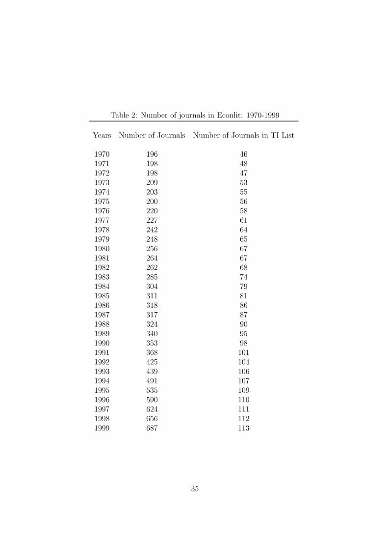
Table 2: Number of journals in Econlit: 1970-1999

Years Number of Journals Number of Journals in TI List

1970 196 461971 198 481972 198 471973 209 531974 203 551975 200 561976 220 581977 227 611978 242 641979 248 651980 256 671981 264 671982 262 681983 285 741984 304 791985 311 811986 318 861987 317 871988 324 901989 340 951990 353 981991 368 1011992 425 1041993 439 1061994 491 1071995 535 1091996 590 1101997 624 1111998 656 1121999 687 113

35

Table 3: Summary statistics for all articles in Econ-Lit.

period 70’s 80’s 90’stotal papers 62569 95027 156454

mean pages per paper 12.85 14.45 16.49standard deviation (9.94) (10.27) (10.59)

# Authors per paper: Distributionsingle-authored .753 .678 .578two authors .210 .256 .309three authors .031 .055 .090four or more authors .005 .011 .023

Table 4: Summary statistics for all articles in 113selected journals (TI list).

period 70’s 80’s 90’stotal papers 26802 38133 52469

mean pages per paper 12.17 13.76 16.29standard deviation (8.69) (8.40) (9.08)

# Authors per paper: Distributionsingle-authored .716 .616 .504two authors .244 .311 .371three authors .035 .064 .104four or more authors .005 .009 .020

36

Table 5: Network statistics for the network based on all arti-cles in EconLit.

period 70’s 80’s 90’stotal authors 33770 48608 81217

mean papers per author 2.35 2.65 2.83standard deviation (3.18) (3.65) (4.10)max papers per author 89 101 129

size of giant component 5253 13808 33027as percentage .156 .284 .407

second largest component 122 30 30

isolated authors 16735 19315 24578as percentage .496 .397 .303

mean links per author .894 1.244 1.672standard deviation (1.358) (1.765) (2.303)max links per author 25 35 54

mean size 10-neighborhood .007 .037 .118clustering coefficient .193 .182 .157

Giant componentmean papers per author 4.80 4.63 4.48standard deviation (5.91) (5.53) (5.67)

percentage coauthored .410 .476 .541

mean links per author 2.48 2.77 3.06standard deviation (2.09) (2.40) (2.93)

mean distance 12.86 11.07 9.47standard deviation (4.03) (3.03) (2.23)maximum distance (diameter) 40 36 29

mean size 10-neighborhood .288 .456 .712clustering coefficient .136 .151 .136

37

Table 6: Network statistics for the network based on all arti-cles in 113 selected journals (TI list).

period 70’s 80’s 90’stotal authors 14051 19694 28736

mean papers per author 2.45 2.77 2.85standard deviation (3.15) (3.50) (3.57)max papers per author 62 69 49

size of giant component 2775 7283 14368as percentage .197 .370 .500

second largest component 74 32 31

isolated authors 5859 5999 6156as percentage .417 .305 .214

mean links per author 1.058 1.467 1.896standard deviation (1.433) (1.815) (2.224)max links per author 21 27 43

mean size 10-neighborhood .015 .060 .165clustering coefficient .188 .180 .167

Giant componentmean papers per author 4.79 4.39 4.02standard deviation (5.45) (4.89) (4.53)

percentage coauthored .411 .502 .590

mean links per author 2.48 2.70 2.95standard deviation (2.05) (2.25) (2.61)

mean distance 11.99 11.12 9.69standard deviation (4.02) (3.07) (2.35)maximum distance (diameter) 33 31 26

mean size 10-neighborhood .379 .438 .658clustering coefficient .139 .154 .149

38

Table 7: Gini coefficients computedfor several data sets.

period 70s 80s 90s

Whole networkAll journals .659 .619 .585

TI List .609 .559 .524

Network excluding isolated authorsAll journals .324 .367 .404

TI List .329 .366 .394

Giant componentAll journals .381 .395 .420

TI List .378 .385 .402

39

Table 8: Network statistics for the economists with the highest number of links.

Author Papers % Coauthored Links Distance 2 Clust.Coeff

1970s

tollison rd 44 0.955 25 57 0.053heady eo 30 0.833 23 13 0.028feldstein ms 73 0.288 21 40 0.024schmitz a 23 0.870 20 29 0.042smith vk 72 0.514 20 26 0.032

Average top 100 23.87 0.724 11.94 25.67 0.062Average all 2.35 0.243 0.89 0.193

1980s

mccarl ba 36 0.889 35 97 0.022thisse jf 34 0.971 30 80 0.055lee cf 36 1.000 29 106 0.030whalley j 52 0.808 29 44 0.022schmitz a 26 0.846 26 118 0.058

Average top 100 28.42 0.827 16.36 49.80 0.062Average all 2.65 0.315 1.24 0.182

1990s

thisse jf 66 0.970 54 244 0.022lee j 58 0.586 45 158 0.019sirmans cf 67 1.000 41 172 0.045nijkamp p 67 0.940 41 57 0.034michel p 48 0.938 34 169 0.036

Average top 100 37.69 0.849 25.31 99.40 0.043Average all 2.82 0.409 1.67 0.157

40

Table 9: Error and attack tolerance of thenetwork based on all articles in EconLit.

period 70’s 80’s 90’s

Size of the giant component (in perc.)Whole network .156 .284 .407w/o random 2% .149 .276 .398w/o random 5% .137 .263 .389w/o top 2% .002 .067 .256w/o top 5% .000 .001 .001

Average distance within giant componentWhole network 12.86 11.07 9.47w/o random 2% 12.88 11.17 9.58w/o random 5% 12.89 11.21 9.68w/o top 2% 9.26 29.80 19.00w/o top 5% 2.64 5.71 8.91

Average size of 10-neighborhoodWhole network .007 .037 .118w/o random 2% .006 .034 .110w/o random 5% .005 .030 .102w/o top 2% .000 .000 .002w/o top 5% .000 .000 .000

Clustering coefficientWhole network .193 .182 .157w/o random 2% .193 .183 .158w/o random 5% .192 .182 .157w/o top 2% .318 .280 .250w/o top 5% .440 .380 .344

41

Table 10: Simulation experiment on the networks constructedfrom the TI data set by deleting nodes to control for the sizein the network.

period 70’s 80’s 90’sactual adjusted adjusted

total authors 14051 14051 14051mean links per author 1.058 1.038 .920

(.009) (.012)

giant component (as perc.) .197 .213 .173(.007) (.014)

isolated authors (as perc.) .417 .424 .464(.002) (.004)

clustering coefficient .188 .184 .169(.004) (.006)

Giant Component

mean links per author 2.48 2.44 2.35(.02) (.02)

mean distance 11.99 13.74 14.79(.77) (1.52)

maximum distance (diameter) 33 38.8 40.9(4.3) (2.8)

clustering coefficient .139 .146 .130(.005) (.005)

Networks are adjusted by deleting nodes randomly until the size (num-ber of authors) is equal to the base period network. Reported numberson the adjusted networks are based on 10 replications. Standard de-viation in the 10 replications is given in parentheses.

42

Table 11: Simulation experiments on the network based on all articlesin American Economic Review, Brookings Papers on Economic Ac-tivity, Econometrica, Quarterly Journal of Economics, RAND (prev.Bell) Journal of Economics, Review of Economic Statistics and Reviewof Economic Studies1.

period 1975-1989 1985-1999 adj. 12 adj. 23

total authors 5530 5468 5468 5468mean links per author 1.218 1.514 1.431 1.218

size of giant component 1147 1666 1561 1295as percentage .207 .305 .285 .237

(.004) (.006)

second largest component 24 21 22 25(4.4) (8.7)

isolated authors 1803 1252 1372 1721as percentage .326 .229 .251 .315

(.002) (.003)

clustering coefficient .229 .215 .203 .172(.002) (.004)

Giant component

mean links per author 2.52 2.67 2.60 2.44(.01) (.02)

mean distance 10.39 9.49 9.71 10.59(.16) (.46)

clustering coefficient .162 .166 .156 .129(.003) (.005)

1 Authors names are distinguished by their last name and all first and mid-dle initials. Adjusted networks are based on the average of 20 simulations.Standard deviation in the 10 replications is given in parentheses.

2 Adjusted by removing 1−C1/C2 fraction of all links, where C1 is mean links perauthor in the giant component in the 1975-1989 network, and C2 is the meanlinks per author in the giant component in the 1985-1999 network. (Methodof Rosenblat and Mobius (2003))

3 Adjusted by removing links until the mean links per author equals the 1975-1989 network.

43

Table 12: Simulation experiments on the network based on all articlesin American Economic Review, Brookings Papers on Economic Ac-tivity, Econometrica, Quarterly Journal of Economics, RAND (prev.Bell) Journal of Economics, Review of Economic Statistics and Reviewof Economic Studies1.

period 1970-1989 1980-1999 adj. 12 adj. 23

total authors 5869 6219 6219 6219mean links per author 1.327 1.657 1.555 1.327

size of giant component 1880 2730 2567 2172as percentage .320 .439 .413 .349

(.005) (.007)

second largest component 26 24 25 23(5.0) (7.5)

isolated authors 1928 1512 1658 2016as percentage .329 .243 .267 .324

(.002) (.003)

clustering coefficient .177 .171 .161 .138(.003) (.004)

Giant component

mean links per author 2.58 2.75 2.67 2.50(.01) (.02)

mean distance 9.40 9.17 9.39 10.06(.14) (.30)

clustering coefficient .144 .150 .140 .117(.003) (.004)

1 Authors names are distinguished by their last name and first initial. Adjustednetworks are based on the average of 20 simulations. Standard deviation inthe 10 replications is given in parentheses.

2 Adjusted by removing 1−C1/C2 fraction of all links, where C1 is mean links perauthor in the giant component in the 1970-1989 network, and C2 is the meanlinks per author in the giant component in the 1980-1999 network. (Methodof Rosenblat and Mobius (2003))

3 Adjusted by removing links until the mean links per author equals the 1970-1989 network.

44

Table 13: Summary statistics for all articles inAmerican Economic Review, Econometrica, Jour-nal of Political Economy, Quarterly Journal ofEconomics and Review of Economic Studies

period 70’s 80’s 90’stotal papers 5023 4565 3705

mean pages per paper 10.65 13.04 17.47standard deviation (7.73) (9.65) (11.29)

# Authors per paper: Distributionsingle-authored .743 .604 .458two authors .225 .330 .424three authors .029 .059 .099four or more authors .003 .007 .019

Table 14: Summary statistics for all articles in jour-nals that have been covered by EconLit since 1970.

period 70’s 80’s 90’stotal papers 42115 46075 49245

mean pages per paper 12.53 13.79 16.12standard deviation (9.96) (10.24) (11.74)

# Authors per paper: Distributionsingle-authored .753 .674 .587two authors .213 .263 .311three authors .030 .055 .085four or more authors .005 .008 .018

45

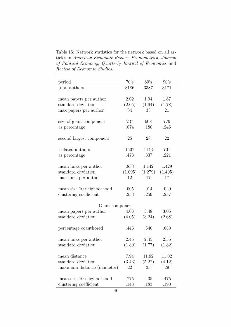
Table 15: Network statistics for the network based on all ar-ticles in American Economic Review, Econometrica, Journalof Political Economy, Quarterly Journal of Economics andReview of Economic Studies.

period 70’s 80’s 90’stotal authors 3186 3387 3171

mean papers per author 2.02 1.94 1.87standard deviation (2.05) (1.94) (1.78)max papers per author 34 33 21

size of giant component 237 608 779as percentage .074 .180 .246

second largest component 25 28 22

isolated authors 1507 1143 701as percentage .473 .337 .221

mean links per author .833 1.142 1.429standard deviation (1.095) (1.279) (1.405)max links per author 12 17 17

mean size 10-neighborhood .005 .014 .029clustering coefficient .253 .259 .257

Giant componentmean papers per author 4.08 3.48 3.05standard deviation (4.05) (3.24) (2.68)

percentage coauthored .446 .540 .680

mean links per author 2.45 2.45 2.55standard deviation (1.80) (1.77) (1.82)

mean distance 7.94 11.92 11.02standard deviation (3.43) (5.22) (4.12)maximum distance (diameter) 22 33 29

mean size 10-neighborhood .775 .435 .475clustering coefficient .143 .183 .190

46

Table 16: Network statistics for the network based on allarticles in journals that have been covered by EconLit since1970.

period 70’s 80’s 90’stotal authors 22960 27539 32773

mean papers per author 2.33 2.28 2.20standard deviation (3.02) (2.77) (2.62)max papers per author 86 97 122

size of giant component 3076 5899 10054as percentage .134 .214 .307

second largest component 82 57 23

isolated authors 11260 11062 10572as percentage .490 .402 .323

mean links per author .885 1.134 1.386standard deviation (1.312) (1.508) (1.695)max links per author 23 25 30

mean size 10-neighborhood .006 .013 .028clustering coefficient .198 .218 .216

Giant componentmean papers per author 4.78 4.00 3.44standard deviation (5.60) (4.31) (3.83)

percentage coauthored .413 .518 .585

mean links per author 2.45 2.62 2.70standard deviation (2.03) (2.11) (2.18)

mean distance 12.15 12.63 12.33standard deviation (3.75) (3.65) (3.36)maximum distance (diameter) 29 37 34

mean size 10-neighborhood .341 .279 .296clustering coefficient .134 .168 .174

47

Table 17: Comparison across subjects: 1995-19991

Biomedical Physics Maths Computer Sc. Economics

1. Total papers 2163923 98502 587000 13169 1564542. Total Authors 1520251 52909 192000 11994 812173. Mean papers per author 6.4 5.1 4.97 2.55 2.834. Mean authors per paper 3.75 2.53 1.63 2.22 1.565. Mean links 18.1 9.7 2.84 3.59 1.6726. Clustering coefficient .066 .43 .15 .496 .1577. Giant component 1395693 44337 n.a. 6396 33027

% of population 92.6 85.4 60* 57 408. Mean distance 4.6 5.9 9* 9.7 9.479. Max Distance 24 20 12* 31 291 The data for medicine, physics and computer science is taken from Newman (2001c). The data for

biomedical sciences comes from the Medline database and covers publications in referreed journals,the data for physics comes from the Los Almos Archive and covers preprints, the data for computerscience comes from the database NCSTRL, and covers preprints. The data for mathematics comesfrom a database on articles in Mathematical Reviews and covers all papers from 1940 onwards; oursummary numbers are taken from Grossman (2002). The data for mathematics and economics coversthe 1990-1999 period. The data pertaining to mathematics marked with a star relates to the networkwith all papers dating from 1940.

48

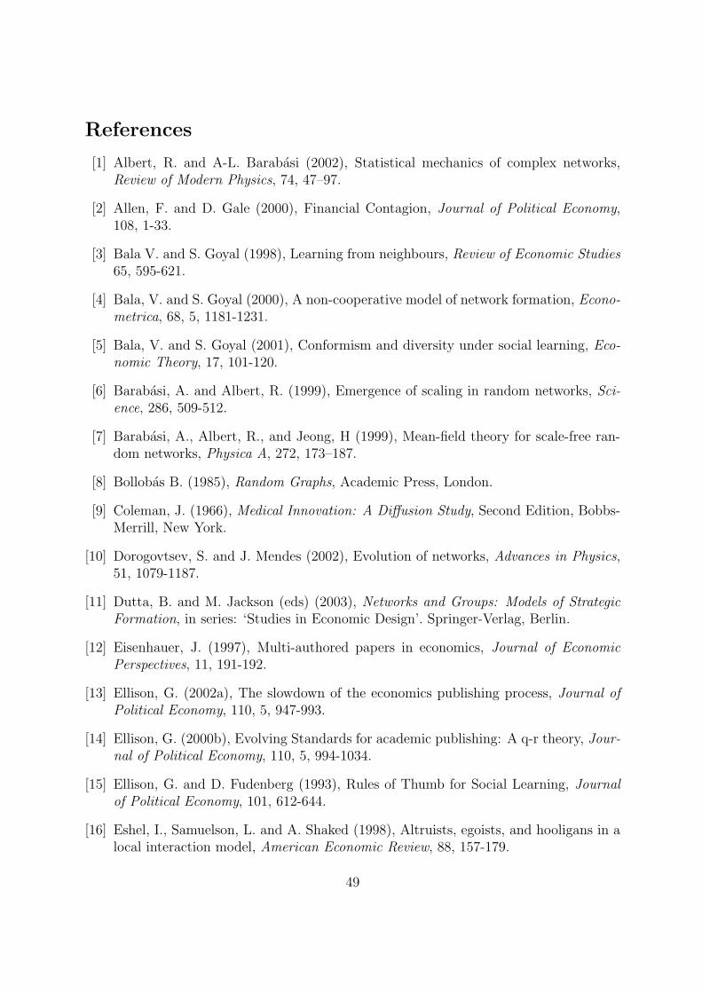
References

[1] Albert, R. and A-L. Barabasi (2002), Statistical mechanics of complex networks,Review of Modern Physics, 74, 47–97.

[2] Allen, F. and D. Gale (2000), Financial Contagion, Journal of Political Economy,108, 1-33.

[3] Bala V. and S. Goyal (1998), Learning from neighbours, Review of Economic Studies65, 595-621.

[4] Bala, V. and S. Goyal (2000), A non-cooperative model of network formation, Econo-metrica, 68, 5, 1181-1231.

[5] Bala, V. and S. Goyal (2001), Conformism and diversity under social learning, Eco-nomic Theory, 17, 101-120.

[6] Barabasi, A. and Albert, R. (1999), Emergence of scaling in random networks, Sci-ence, 286, 509-512.

[7] Barabasi, A., Albert, R., and Jeong, H (1999), Mean-field theory for scale-free ran-dom networks, Physica A, 272, 173–187.

[8] Bollobas B. (1985), Random Graphs, Academic Press, London.

[9] Coleman, J. (1966), Medical Innovation: A Diffusion Study, Second Edition, Bobbs-Merrill, New York.

[10] Dorogovtsev, S. and J. Mendes (2002), Evolution of networks, Advances in Physics,51, 1079-1187.

[11] Dutta, B. and M. Jackson (eds) (2003), Networks and Groups: Models of StrategicFormation, in series: ‘Studies in Economic Design’. Springer-Verlag, Berlin.

[12] Eisenhauer, J. (1997), Multi-authored papers in economics, Journal of EconomicPerspectives, 11, 191-192.

[13] Ellison, G. (2002a), The slowdown of the economics publishing process, Journal ofPolitical Economy, 110, 5, 947-993.

[14] Ellison, G. (2000b), Evolving Standards for academic publishing: A q-r theory, Jour-nal of Political Economy, 110, 5, 994-1034.

[15] Ellison, G. and D. Fudenberg (1993), Rules of Thumb for Social Learning, Journalof Political Economy, 101, 612-644.

[16] Eshel, I., Samuelson, L. and A. Shaked (1998), Altruists, egoists, and hooligans in alocal interaction model, American Economic Review, 88, 157-179.

49

[17] Glaeser, E., B. Sacerdote and J. Scheinkman (1996), Crime and social interactions,Quarterly Journal of Economics, 111, 507-548.

[18] Goyal, S. (1996), Interaction structure and social change, Journal of Institutionaland Theoretical Economics, 152, 3, 472-495.

[19] Goyal, S. (2003), Learning in networks: a survey. mimeo.

[20] Grossman, J (2002), The evolution of the mathematical research collaboration graph,Congressus Numerantium, 158, 201–212.

[21] Hamermesh, D and Oster, S (2002), Tools or toys: The impact of high technologyon scholarly productivity, Economic Inquiry, 40, 539–555.

[22] Hagerstrand, T. (1969), Innovation diffusion as a spatial process. University ofChicago Press. Chicago.

[23] Hudson, J. (1996), Trends in multi-authored papers in economics, it Journal of Eco-nomic Perspectives, 10, 153-158.

[24] Jackson, M. (2003), A survey of models of network formation: Stability and efficiency.mimeo.

[25] Jackson, M. and A. Wolinsky (1996), A strategic model of economic and social net-works, Journal of Economic Theory, 71, 44-74.

[26] Kochen, M. (ed) (1989), The small world, Ablex, Norwood, NJ.

[27] Kranton, R. and D. Minehart (2001), A theory of buyer-seller networks, AmericanEconomic Review, 91, 485-508.

[28] Laband, D. and Tollison, R. (2000), Intellectual collaboration, Journal of PoliticalEconomy, 108, 3, 632-662.

[29] McDowell, J.M., and Melvin, M. (1983), The determinants of co-authorship: Ananalysis of the economics literature, Review of Economics and Statistics, 65, 1, 155–160.

[30] Milgram, S. (1967), The small world problem, Psychology Today, 2, 60-67.

[31] Morris, S. (2000), Contagion, Review of Economic Studies, 67, 57-79.

[32] Newman, M. (2003), Coauthorship networks and patterns of scientific collaboration,Proceedings of the National Academy of Sciences, in press.

[33] Newman, M. (2001a), Scientific collaboration networks: I. Network construction andfundamental results, Physical Review E, 64.

50

[34] Newman, M. (2001b), Scientific collaboration networks: II. Shortest paths, weightednetworks, and centrality, Physical Reviews E, 64.

[35] Newman, M. (2001c),The structure of scientific collaboration networks, Proceedingsof the National Academy of Sciences, 98, 404-409.

[36] Pool, I de Sola. and Kochen, M. (1978), Contacts and Influence, Social Networks, 1:1-48.

[37] Ravasz, E. and A.-L. Barabasi (2003), Hierarchical organization in complex networks,Physical Review E, 67, art. 026112.

[38] Rosenblat, T. and M. Mobius (2003), Getting closer or drifting apart? mimeo.

[39] van den Nouweland, A. (2003), Models of network formation in cooperative games.mimeo.

[40] Watkins, S. (1991), Provinces into Nations: Demographic Integration in WesternEurope, 1870-1960, Princeton University Press, Princeton, New Jersey.

[41] Watts, D. (1999), Small Worlds: The Dynamics of Networks between Order andRandomness, Princeton University Press, Princeton, New Jersey.

[42] Watts, D. and Strogatz, S. (1998), Collective dynamics of ‘small world’ networks,Nature, 393, 440–442.

[43] Young, P. (1998), Individual Strategy and Social Structure, Princeton UniversityPress, NJ.

51

Figure 1: Pareto plot of links per author for the network based on all articles: 1970s to1990s.

Figure 2: Lorenz curves of links per author for the network based on all articles: 1970sto 1990s.

Figure 3: Neighborhood of network around J. Stiglitz in the 1990’s.

Figure 4: Neighborhood of network around J. Tirole in the 1990’s

Figure 5: Neighborhood of network around J.F. Thisse in the 1990’s

Figure 6: Neighborhood of network around A. Dixit in the 1990’s

Figure 7: Fraction of coauthored articles in AA journals, A journals, B journals and otherjournals.

Figure 8: Equilibrium networks

Figure 9: Equilibrium networks with size constraints.

Figure 10: Degree versus clustering.

Figure 11: The construction of a hierarchical network. Source: Ravasz and Barabasi(2003)

52

Figure 1

Figure 2

Figure 3: Local network of J. Stiglitz in 1990’s

Note: Some economists might appear twice or are missing due to the use of different initials or misspellings in EconLit.

Figure 4: Local network of J. Tirole in 1990’s

Note: Some economists might appear twice or are missing due to the use of different initials or misspellings in EconLit.

Figure 5: Local network of J. Thisse in 1990’s

Note: Some economists might appear twice or are missing due to the use of different initials or misspellings in EconLit.

Figure 6: Local network of A. Dixit in 1990’s

Note: Some economists might appear twice or are missing due to the use of different initials or misspellings in EconLit.

Figure 7Collaboration across journals

Figure 8: Symmetric equilibrium networks

nh=3 & nl=6

fll<f<fhhf>fhh

Lηhh=2

f<fll

H H

HH

L LL

LL L

L

L

L

LL

L

HL

HLL

LL

HH

Empty network Clique of High Types + isolated low types

ηll=1Hηhh=2

Separate cliques

Figure 9: Symmetric equilibrium networkswith size constraints.

nh=3 & nl=6flh<f<fhhηhh>nh-1f>fhh

L

H H

L LL

LL L H

LHLH L

HL L

Empty network Clique of High Types

f<fllfll<f<flh

H

H

L

H

H

LL L

L LHLL

LH

L LLInterlinked stars Interlinked stars + high clustering

Figure 10Degree vs clustering

Figure 11 The construction of a hierarchical network

(a) 1 level, n=5

(b) 2 levels, n=25 (c) 3 levels, n=125