economic regulation in power distribution · 2017-05-12 · ted generation (dg) is connected to...

ECONOMIC REGULATION IN POWER DISTRIBUTIONREPORT 2017:362

RISK- OCH TILLFÖRLITLIGHET

Economic Regulation in Power Distribution Economic Regulation Impact on Electricity Distribution

Network Investment Considering Distributed Generation

YALIN HUANG

ISBN 978-91-7673-362-2 | © ENERGIFORSK March 2017

Energiforsk AB | Phone: 08-677 25 30 | E-mail: [email protected] | www.energiforsk.se

ECONOMIC REGULATION IN POWER DISTRIBUTION

3

Foreword

In the future, more distributed generation will be connected to distribution and regional electrical networks. One of the EU's climate goals for 2020 is that 20% of EU electricity consumption will come from renewable electricity that mostly is from distributed generation. A lot of the investment in renewable electricity production in Sweden will probably be in the wind, because the Energy Agency proposed a planning target of 30 TWh of wind power by the year 2020. Given the network owners technical requirements, power generators independently decide which investments should be implemented and where to connect the distributed generation to distribution and regional network. The network owners must enable connection of distributed generation and also meet the requirements of power quality and reliability at a reasonable cost. An uncertainty is connected with the distributed generation. How will it affect the network companies network planning?

This project analyze how the distributed generation affects the reliability and the consequences of power outages.

Yalin Huang from the Royal Institute of Technology has been the project manager for the project. She has worked together with Lennart Söder who is professor in Electric Power Systems at KTH.

Many thanks to the program board for good initiative and support. The program Board consisted of the following persons:

• Jenny Paulinder, Göteborg Energi (Chairman)• Lars Enarsson, Ellevio• Jonas Alterbäck, Svk• Hans Andersson, Vattenfall Distribution• Kenny Granath, Mälarenergi Elnät• Par-Erik Petrusson, Jämtkraft• Magnus Brodin, Skellefteå Kraft Elnät• Ola Löfgren, FIE• Anders Richert, Elsäkerhetsverket• Carl Johan Wallnerström, Energimarknadsinspektionen• Susanne Olausson, Energiforsk (Program manager)

The following companies have been involved as stakeholders in the project. A big thanks to all the companies for their valuable contributions.

• Ellevio AB• Svenska kraftnät,• Vattenfall Distribution AB• Göteborg Energi AB,• Ellinorr AB• Jämtkraft AB,• Mälarenergi Elnät AB,• Skellefteå Kraft Elnät,• AB PiteEnergi,

ECONOMIC REGULATION IN POWER DISTRIBUTION

4

• Energigas Sverige,• Jönköping Energi Elnät AB• Boras Elnät AB• Föreningen för Industriell Elteknik, FIE

Stockholm, January 2017

Susanne Olausson Energiforsk AB Research Area Electrical networks, Wind and Solar electricity

Summary

One of EU’s actions against climate change is to meet 20% of energy consumption

from renewable resources by the year 2020 when the project was started. Now this

target has increased to at least 27% by the year 2030. In addition, given that the

renewable resources are becoming more economical to generate electricity from

and that these resources are distributed geographically, more and more distribu-

ted generation (DG) is connected to power distribution. The increasing share of

DG in the electricity networks implies re-distribution of costs and benefits among

distribution system operators (DSOs), customers and DG owners. How the costs

and benefits will be allocated among them depends on the established economic

regulation.

The established economic regulation regulates the DSOs’ revenue and perfor-

mances. The time when the DSOs are remunerated based on their actual costs has

passed. Nowadays the economic regulation is in place to steer efficient investments.

Network investments are no longer just to satisfy the load growth, or to higher the

investments does not bring higher revenue. Network investments are incentivised

by the regulation to be more efficient. Furthermore, the potential of DG to defer

network investment is widely recognized in the regulation. Ignoring this potential

of DG may decrease DSOs’ efficiency. Last but not the least, network unbundling

is a common practice in Europe. Ignoring the fact that DSOs and DG owners are

different decision makers in studies can lead to inaccurate analysis.

Driven by the target of a higher DG integration and more efficient investments

in the unbundled distribution networks, proper economic regulations are needed

to facilitate this change. The objective of this project is to evaluate the impact

from regulations on distribution network investment considering DG integration.

In other words, this project aims to develop methods assist regulators to design

desirable regulations to encourage the DSOs to make the “smart” decisions. In

order to achieve that, a modelling approach is proposed to quantify the economic

regulation impacts and the benefit of innovative investments. Regulations are en-

coded into the network investment model. The developed models, in other words,

assist DSOs to make the “right” investment in the “right” place at the “right”

time under the given regulation.

2

Sammanfattning

Mer och mer distribuerad generering kommer i framtiden anslutas till lokal- och

regionnaten. Ett av EU:s klimatmal till ar 2020 ar att 20 % av EU:s elkonsumtion

ska komma fran fornyelsebar elproduktion som till stor del bestar av distribu-

erad generering. Manga av investeringarna i fornyelsebar elproduktion i Sverige

kommer troligtvis att ske i vindkraft, eftersom Energimyndigheten har foreslagit

ett planeringsmal pa 30 TWh vindkraft till ar 2020. Natagarna ska mojliggora

anslutning av distribuerad generering samtidigt som de maste uppfylla krav pa

elkvalitet och tillforlitlighet till en rimlig kostnad. Osakerheten i var distribuerad

generering ansluts kommer att paverka elnatsforetagens natplanering. Den okade

andelen distribuerad generering i lokal- och regionnaten kommer att medfora bade

okade kostnader och okade vinster for natagare, kunder och elproducenter. Hur

mycket distribuerad generering som ansluts och hur kostnader och vinster ska

fordelas mellan aktorerna i elbranschen kommer till en stor del att avgoras av vil-

ka regelverk som upprattas.

Vilka blir de ekonomiska konsekvenserna av olika strategier for natutbyggnad for

distribuerad generering? Ska en natagare fa ekonomiska incitament for att ha va-

rit kostnadeffektiv? Hur kompenseras producenter vid bortkoppling? Alla dessa

fragestallningar beror pa vilken avkastning regleringen tillater samt hur andra de-

lar av regleringen utformas. I detta projekt har matematiska metoder som kan

ta hansyn till osakerheter kring hur mycket distribuerad generering som kommer

att anslutas till naten har utvecklats for att utvardera investeringsalternativ. Med

hjalp av de utvecklade metoderna kan den optimala natutbyggnaden givet en viss

reglering identifieras. Man kan darmed fa en battre uppskattning av vilken utbygg-

nad man far beroende pa hur natregleringen ar utformad. Dessutom kan man med

dessa metoder utreda hur natregleringen paverkar natinvestering och foresla mer

effektiv natreglering.

3

Contents

1 Introduction 1

2 Regulation on distribution systems with distributed generation 8

2.1 Revenue cap regulation . . . . . . . . . . . . . . . . . . . . . . . . . 9

2.2 Performance regulation . . . . . . . . . . . . . . . . . . . . . . . . . 11

2.3 Curtailment regulation . . . . . . . . . . . . . . . . . . . . . . . . . 13

2.4 Connection charge regulation for DG . . . . . . . . . . . . . . . . . 14

3 The developed network investment optimisation model (NIOM) 15

3.1 Modelling of input data uncertainties . . . . . . . . . . . . . . . . . 16

3.1.1 Motivation for the chosen modelling approach . . . . . . . . 16

3.1.2 Modelling the input uncertainties with correlations . . . . . 17

3.2 Modelling of regulations . . . . . . . . . . . . . . . . . . . . . . . . 18

3.2.1 Modelling of revenue cap regulation . . . . . . . . . . . . . . 20

3.2.2 Modelling of performance regulation . . . . . . . . . . . . . 20

3.2.3 Modelling of DG curtailment . . . . . . . . . . . . . . . . . 24

3.2.4 Modelling of DG connection and unbundling regulation . . . 25

3.2.5 A summary of the models . . . . . . . . . . . . . . . . . . . 25

3.3 Formulation of the developed NIOM . . . . . . . . . . . . . . . . . 26

3.3.1 Variables . . . . . . . . . . . . . . . . . . . . . . . . . . . . . 26

3.3.2 Objective function . . . . . . . . . . . . . . . . . . . . . . . 27

3.3.3 Technical constraints . . . . . . . . . . . . . . . . . . . . . . 28

3.4 Modelling of reliability . . . . . . . . . . . . . . . . . . . . . . . . . 31

4 The developed network investment assessment model (NIAM) 33

4.1 Modelling of line capacity . . . . . . . . . . . . . . . . . . . . . . . 33

4

CONTENTS

4.1.1 Standard line capacity calculation . . . . . . . . . . . . . . . 33

4.1.2 Calculation of static line rating (SLR) . . . . . . . . . . . . 34

4.1.3 Calculation of dynamic line rating (DLR) . . . . . . . . . . 35

4.2 Formulation of the developed NIAM . . . . . . . . . . . . . . . . . 36

5 Application of developed models 40

5.1 Application of NIOM . . . . . . . . . . . . . . . . . . . . . . . . . . 40

5.1.1 Case study for incentive regulation . . . . . . . . . . . . . . 40

5.1.2 Case study for curtailment regulation . . . . . . . . . . . . . 43

5.2 Application of NIAM . . . . . . . . . . . . . . . . . . . . . . . . . . 49

5.2.1 Case study for evaluating investment in DLR . . . . . . . . 50

6 Conclusions 54

6.1 Case study implications . . . . . . . . . . . . . . . . . . . . . . . . 55

5

Chapter 1

Introduction

Economic regulation in power systems

Regulation conveys different meanings in different contexts in power systems. It

can appear in the context of security or the environment as social regulation [1],

where regulation seeks to protect workers’ safety and the environment. It can

appear in the context of power system operation as frequency regulation. This

kind of regulation seeks to maintain the balance between generation and load. It

can appear in the context of electricity market, the network investment supervision

and network tariff designs as economic regulation. In this project, the economic

regulation in power distribution is the focus. The following elements are defined

as the basic scope of economic regulation in power systems [1]:

• The design of rules for steering agents’ behaviour towards the objectives de-

fined by the regulator.

• The definition of the structure of the power industry, e.g. a vertically inte-

grated or unbundled structure. For either structure, an appropriate business

model is needed.

• The supervision of agents’ behaviour. This involves reviewing their effective-

ness to achieve the defined objectives and taking legal actions.

The agents, in power systems, are referred to as utilities or service providers

in the electricity industry. Traditionally power systems were vertically integrated

1

CHAPTER 1. INTRODUCTION

world wide. In this type of structure, one utility has the monopoly on all functions

from generation, transmission to distribution in power systems. These functions

are illustrated in Fig. 1.1. The voltage levels for transmission and distribution

lines differ among countries. The price of electricity is regulated. The utility’s

investment and operating practices are supervised by the government regulator.

TransmissionUlinesU765RU500RU345RU230RUandU138UkV

TransmissionUCustomer138kVUorU230kV

GeneratingUStation

GeneratingStepUUp

Transformer

SubstationStepUDown

TransformerGeneration

Green:Blue:

SubtransmissionCustomer

26kVUandU69kV

PrimaryUCustomer13kVUandU4kV

SecondaryUCustomer120VUandU240V

TransmissionDistribution

ColorUKey:Red:U

CustomerBlack:U---->

---->

Figure 1.1: Simple diagram of electricity grids [2].

Since the end of the last century this traditional structure has changed in

many countries. Chile started this process in 1982, followed by England and

Wales, Norway, Sweden and some countries in South America. The main con-

tent of this change was to introduce market platforms for electricity trade [1].

Electricity wholesale markets and retail markets have been introduced for the

electricity production and retail activities respectively. However, the transmission

and distribution networks have remained to be monopolies, which are owned by ei-

ther independent organisation, private investors, municipalities or the government.

Therefore, electricity generation and trading are unbundled from the network ac-

tivities. The “agents” in the unbundled power systems are referred to all service

providers of the electricity generation, transmission, wholesale, distribution, retail,

etc. The regulators can be an authority or a public body or a private body inde-

pendent from the interests of the electricity industry according to the EU directive

[3]. This change requires modification in power system planning and operation. It

also requires new economic regulation for steering electricity market’s and network

companies’ behaviour and new rules to review the effectiveness.

A distinction is drawn between the regulation for the electricity market and the

network companies which are categorised as natural monopolies [4]. Regulation for

the electricity market aims to ensure a competitive trading platform, for example,

2


a minimum number of competitors, to correct monopolistic markets or imperfect

information [1]. Regulation for network companies aims to ensure the economic

and financial sustainability of the companies, and productive efficiency [4]. In other

words, the regulation for network companies aims to ensure that the companies

offer the lowest possible price without going bankrupt in the long-term. This

project focuses on the area of regulation for network companies.

Many regulatory variables to assist the regulator to reach this goal are found

in practise. One is the regulation of the revenues. The allowed revenues should be

high enough to sustain the company and should not be so high that the consumers

pay unjustifiably high prices. Another variable is to set quality standards and

performance incentives. Quality standards are the requirements that the utilities

have to meet. For example, reliability of supply, the voltage quality, etc. These re-

quirements can be linked to the regulation of the revenues. Performance incentives

are economic incentives to encourage the company perform better. For example,

reducing the thermal losses in the network. Performance incentives can also be

linked to the revenue regulation.

Many deregulated power systems have moved from the traditional cost-of-

service regulation to incentive-based regulation on the revenue. In cost-of-service

regulation, also known as rate-of-return regulation, the revenue that a network

company is allowed to receive is based on the total cost, where the investment cost

is compensated by an allowed rate-of-return set by the regulator [1]. The tariffs

charged by the company are also set by the regulator. This regulation is im-

plemented with slightly variations in different systems. However, incentive-based

regulation is implemented in very different forms. The most common form is the

revenue cap regulation, such as in Austria, Spain and Sweden, [5]. Under this

design, the maximum yearly revenue of a company for a certain period is set by

the regulator. The revenue target is set based on the historical performance with

some efficiency measures and inflation adjustment.

Under the cost-of-service regulation, the increase of cost leads to a higher rev-

enue and a higher profit of the utility as demonstrated in Fig. 1.2a. Two scenarios

are demonstrated in this figure, one is the scenario where the cost increases; the

other one is the scenario where the cost decreases. The profit is the difference be-

tween the revenue and the cost, which is marked by a shaded area in the figure. If

the cost decreases, the profit decreases as well in Fig. 1.2a. Therefore, the cost-of-

3


service regulation is not encouraging any “smart” investment. However, under the

revenue cap regulation, if the cost increases more than the efficiency requirement,

as indicated by the solid red line and dotted red line respectively in Fig. 1.2b,

the profit decreases. If the company can improve the efficiency better than the

regulator expected, which is indicated by the lower dashed red line, the profit for

the company increases. The “extra” profit due to the extra efficiency improvement

is indicated by the black strips. Therefore, the company has a significant incentive

to reduce the cost.

Time

€Revenue

CostProfit

Time

€

Revenue

CostProfit

T

T

(a) Profits under cost-of-service regulation.

Time

€Revenue

CostProfit

Time

€

Revenue

CostProfit

T

T

(b) Profits under revenue cap regulation.

Figure 1.2: DSO’s profit over time under different economic regulations.

Another form of the incentive-based regulation is the price cap regulation, for

example in the United Kingdom a few years ago[5]. In the price cap regulation, the

maximum price that the company can charge the consumers is set by the regulator.

It provides incentives to reduce costs as in the revenue cap regulation; however, it

also provides incentives to increase electricity sales [4]. The increase of electricity

sales may have little impact on the network infrastructure cost; therefore, with

higher sales the company can receive a higher revenue and consequently a higher

profit. Therefore, the price cap regulation is less compatible with energy efficiency

goals than the revenue cap regulation.

In the incentive-based regulation, the high focus on the cost reduction may lead

to deterioration of the quality of service. Therefore, other two regulatory variables,

quality standards and performance incentives, are often applied to complement it

[4]. If the company fails to satisfy the quality standards, it can lead to penalties.

4


Performance incentives can be positive or negative. They are often integrated in

the revenue cap setting formula. A company’s revenue cap may be increased or

decreased depending on the performance incentives. Regulators need to define the

correct and effective incentives to steer the performance. Therefore, methods to

model different performance incentives, economic regulatory framework and the

network investment are necessary for regulators to analyse the regulation impact

on network cost and performances.

Distributed generation

Not only the regulation schemes changed in power systems in the recent years,

power flows in the system have also changed. With the liberalisation of electricity

markets and environmental concerns, distributed generation (DG) has developed

rapidly [6]. With the development of technologies, the cost of DG units decreases.

This also contributes to a further increase of DG installation [7]. The definition

of DG in [8] is adopted in this project, which is an electric generation source

connected directly to the distribution network or on the customer side of the

meter. DG can be renewable generators like wind power plants and solar power

plants, and traditional generators like gas turbines and fuel cells [6].

Traditionally the power in the power system flows only in one direction, from

central power plants to transmission network then to distribution network, and

down to consumers. The power in the power system can now flow from the con-

sumer end back to the distribution network and even to the transmission network,

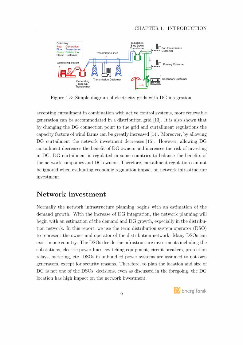
as shown in Fig. 1.3. On the one hand, DG connection to the grid entails in-

vestment in new network infrastructure. It may also entail reinforcement in the

existing network. On the other hand, DG integration has shown benefits of defer-

ring network investment [9, 10, 11]. However, the deferment of investments and

the schedule of reinforcements are highly sensitive to DG locations [12]. The ben-

eficial impact on deferring the investment in the system may be diluted because

of the “wrong” timing and location of DG. Therefore, DG integration should be

taken into account in the network infrastructure investments.

The benefit of DG integration can be higher if DG curtailment is accepted [13,

14]. The amount of curtailed energy is closely related to the DG connection point,

the connection line investment and the network reinforcement and operation. By

5


Transmission lines

Transmission Customer

Generating Station

GeneratingStep Up

Transformer

SubstationStep DownTransformer

Generation

Green:Blue: Sub transmission

Customer

Primary Customer

Secondary Customer

TransmissionDistribution

Color Key:Red:

CustomerBlack: ---->

---->

---->

Figure 1.3: Simple diagram of electricity grids with DG integration.

accepting curtailment in combination with active control systems, more renewable

generation can be accommodated in a distribution grid [13]. It is also shown that

by changing the DG connection point to the grid and curtailment regulations the

capacity factors of wind farms can be greatly increased [14]. Moreover, by allowing

DG curtailment the network investment decreases [15]. However, allowing DG

curtailment decreases the benefit of DG owners and increases the risk of investing

in DG. DG curtailment is regulated in some countries to balance the benefits of

the network companies and DG owners. Therefore, curtailment regulation can not

be ignored when evaluating economic regulation impact on network infrastructure

investment.

Network investment

Normally the network infrastructure planning begins with an estimation of the

demand growth. With the increase of DG integration, the network planning will

begin with an estimation of the demand and DG growth, especially in the distribu-

tion network. In this report, we use the term distribution system operator (DSO)

to represent the owner and operator of the distribution network. Many DSOs can

exist in one country. The DSOs decide the infrastructure investments including the

substations, electric power lines, switching equipment, circuit breakers, protection

relays, metering, etc. DSOs in unbundled power systems are assumed to not own

generators, except for security reasons. Therefore, to plan the location and size of

DG is not one of the DSOs’ decisions, even as discussed in the foregoing, the DG

location has high impact on the network investment.

6


Before the first DG connection, the cost of the network is recovered by network

charges from all consumers. Due to DG connection, reinforcement in the exist-

ing network may increase. The reinforcement cost can be transferred to only the

DG owner, or can be socialized by all the network users. Depending on how the

connection fee for DG is charged, DG owners can choose the connection point to

the grid while accepting the probability of energy curtailment at this point. For

example, the income of a DG owner is from the sell of the generated energy, and

from compensation from the curtailed energy if it is applicable. The connection

cost of a DG owner can be due to the connection line only or due to the connection

line and the reinforcement of the existing grid. If the DG owner tries to maximise

its income or minimise the connection cost, different regulation on curtailment and

connection charge can have a direct impact on the decision. Therefore, an inves-

tigation of the relationship between economic regulation and network investment

interests DG developers as well.

Aim and scope of the project

The main objective of this project is to evaluate the impact from regulations on

the distribution network investment. In other words, this project aims to develop

methods to assist regulators to design desirable regulations to encourage the DSOs

to make the “smart” decisions; and to assist DSOs to build the “right” line in the

“right” place at the “right” time considering the current regulation.

7

Chapter 2

Regulation on distribution

systems with distributed

generation

DSOs are natural monopolies, so their revenues and performances have to be reg-

ulated. Traditionally, the revenue of the DSO is based on cost-of-service, also

called rate-of-return scheme, where a predefined rate of return on the capital in-

vestment is guaranteed and other operational costs are passed through. There is

then little incentive for the DSO to minimize the costs. To improve the economic

efficiency, traditional revenue regulation model is not suited any more, one solu-

tion is to implement incentive regulation, which includes revenue cap regulation

and/or performance regulation.

Moreover, in Europe, the unbundling rules, according to the Article 14/7 of

the Directive 2003/54/EC [12], prohibit DSOs from owning generation plants. At

the same time, it is recommended that when planning the distribution network,

DG that might replace the need to upgrade electricity capacity shall be considered

by the DSO. Research has shown that DG can reduce the system losses, improve

voltage profile, enhance system reliability etc [16, 17]. Therefore, regulations of

DSOs should recognize the impact of DG on DSOs’ performance and cost[5].

The growth of distributed generation (DG) is adding complexity to the dis-

tribution network investment and network regulation. Different connection fee

schemes can impact the DSO’s network investment decision and the DG owners’

8

CHAPTER 2. REGULATION ON DISTRIBUTION SYSTEMS WITHDISTRIBUTED GENERATION

decisions[5]. Connection charge fee schemes allocates the costs and risks between

DG producers and DSOs [18]. Moreover, DG integration is especially challenging

for the generation from renewable energy with high variability. The network in-

vestment can be based on accommodating the energy produced from DG without

curtailment; however, a part of these investments might be only relevant for a

few hours annually when the generation is much higher than the average. There-

fore, energy curtailment is an option to decrease the investment [19]. However,

energy producers may suffer economic losses due to curtailment. Furthermore,

curtailing renewable energy can intuitively be viewed as noneconomical given its

low marginal cost. Therefore, curtailed producers may receive compensation ac-

cording to energy curtailment regulation, which defines the compensation rules in

terms of the price, the quantity and the payer. Energy curtailment can be caused

by network constraints, security constraints in the grid, low electricity price, and

strategic bidding [20]. The curtailment of DG due to network constraints is the

focus of this thesis.

2.1 Revenue cap regulation

Under the revenue cap regulation, the maximum yearly revenue that the DSO

is allowed to earn in a year is limited by the revenue from the previous year

considering inflation and performance for a period of several years [4]. These

revenues are adjusted annually due to unexpected events, e.g. extreme weather.

The revenue cap regulation can also be implemented considering DG integration.

There are several proposals in [21] [22] [23] to adjust the allowed revenue for DSOs

in order to encourage them to connect more distributed energy resources (DERs).

DG integration is a part of DER integration. Other DERs can be distributed

energy storage and electric vehicles.

In general, there are three ways to adjust the allowed revenue for DSOs to

facilitate DER integration, which are presented in eq.(2.1) [24]. The DSO is incen-

tivized by an increase of their revenue cap by connecting more DER. The compo-

nent can be one of three elements: a percentage of the total DER connection cost

(α), an average reward for connected DER capacity (β) or an average reward for

DER generation (γ). In some proposed regulatory schemes in [25], the additional

component can be a combination of those three elements.

9


Rt = Rt−1 ∗ adjustment factor +

α·eDER α : (%),

β · PDER β : (e/kW ),

γ ·GDER γ : (e/MWh).

(2.1)

where Rt represents the revenue cap in year t, adjustment factor is usually set

by the regulators according to the economic indexes, eDER represents the DER

connection cost, PDER represents the total installed capacity of DER, and GDER

represents the generation from DERs.

In practice, excess revenue is returned to customers in some way, so that the cap

is achieved ex post [26]. This is also known as a revenue-sharing scheme. Another

way to share profit with consumers is called the sliding scale method which avoids

a certain level of information asymmetry [21]. The sharing rules is presented in

(2.2).

R = b ∗ revenue cap + (1− b) ∗ cost (2.2)

In Sweden, revenue cap regulation is applied but there is no special incentives

for DER integration. The incentives focus on quality and performances. The

components in the Swedish revenue cap for the current regulatory period of years

2016-2019 is illustrated in Figure 2.1 [27]. The DSOs provide information about

their costs and performances to the regulator. The regulator defines the parameters

to calculate the revenue cap. Efficiency change defines the efficiency improvement

requirement on the operations. Depreciation method describes how to depreciate

the capital cost. Return of capital is defined to reward the capital investment.

The quality and network utilization indices are used to quantify the incentives for

qualified and efficient network investment. The revenue cap is calculated for each

DSO based on its cost and performances.

The revenue cap defines the maximum total revenue that a DSO can receive for

the regulatory period. The calculation for the allowed return on costs is presented

in [27], the performance incentive from the quality regulation is presented in [28],

and the calculation and motivation for the performance incentives from network

utilization are presented in [29]. A realistic evaluation of the regulatory asset

10


base is crucial. In Sweden, a standard cost catalogue is implemented [30]. The

catalogue shows standard replacement costs for specific assets.

DSO’s input • Controllable cost

Regulator’s input

• Efficiency change

Regulator’s output

• Revenue cap = Allowed return on costs + Adjusted incentives (quality andnetwork utilization)

• Non-controllablecost

• Capitalbase

• Performancemeasures

(Quality and network utilization)

(Quality and network utilization)

• Depreciation • Return ofcapital

• Performanceindices

Figure 2.1: Swedish revenue cap regulation framework.

2.2 Performance regulation

In the performance regulation, choosing performance indicators is one of the chal-

lenges. Qualitative analysis on different performance indicators, used in European

countries and proposed ones, are presented in [31]. Some guidelines are also given

by CEER in [31]. CEER selected some performance indicators for further quali-

tative analysis in [32]. The selection criteria of performance indicators are:

1. The variation would determine a quantifiable benefits to grid users and in

general, society as a whole;

2. It is possible to determine, measure of calculate, the value of the index in a

sufficiently accurate and objective way;

3. The value of the index can be influenced (even if to a limited extent) by the

network operator or the system operator; this includes metering;

4. The index should be as far as possible, technology neutral.

11


The performance indicators implemented from January 2016 in Sweden fulfils

all the above criteria and send out incentives to facilitate demand side manage-

ment (DSM) and innovative solutions. They, which have not earlier been analysed

quantitatively in a systematic manner, are modelled and analysed in this thesis.

The performance incentives for distribution networks utilization in Sweden are

calculated based on two performance indicators [29]. One is to motivate the DSO

to reduce losses in the network, the other is to motivate the DSO to increase the

load factor.

Network losses can be affected by the DSO’s investment decision. An incentive

to reduce the losses can benefit the network users, since the cost of losses will

be recuperated from them; and can benefit the society, since less energy will be

produced to cover the losses. The economic incentive from loss reduction is shared

by the DSO and the customers. The ratio to share is determined by the regulator.

A similar formulation of incentives for loss reduction can be found in some other

European countries, for example Austria and Spain [32].

The load factor of the network is the ratio between the average power and the

peak power on the feeding point (or connection point) of a distribution network.

It is considered as an index for efficient utilization of the networks in the Swedish

regulation. This is because one effective way of using the network is to level off

the flow profiles, considering there is load and generation in the network. The load

factor defined in the Swedish regulation is the yearly mean value of the daily ratios

during a regulatory period. The higher the ratio is, the smaller the flow variation

on average is during each day. Therefore, the capacity of the network is used more

efficiently. This incentive aims to encourage DSOs to recognize the contribution

from the DG or DSM to the network.

By levelling off the flows in the network, the peak power in the network and

also the losses can be reduced, giving the total energy unchanged. Therefore, it can

lead to network investment reduction. The loss reduction can be doubly rewarded

by these two incentives. However, they are still different incentives. The loss

reduction incentive provides a static value for the loss reduction at any time; the

loss reduction in the peak load moments provides a more dynamic value for the loss

reduction. Therefore, the loss reduction at times of peak load is more beneficial

than that at other times. This reflects different benefits of the loss reduction at

different times.

12


The performance of the DSO depends not only on DSO’s investment decision,

but also on objective reasons such as the geography of the network, the types

of consumer or DG and the size of the company. In order to limit the impact

of the objective reasons, the Swedish regulator sets a limit on the sum of the

economic incentives each DSO can obtain. More detailed settings in the Swedish

performance regulation are presented in Chapter 3.2.

2.3 Curtailment regulation

Curtailment in this thesis is defined as the difference between the energy that

is potentially available from the generation unit and the energy that is actually

produced. The reasons for curtailment can be categorized into four kinds: network

constraints, security constraints in the grid, excess generation relative to load

and strategic bidding [20]. In the distribution level, the most relevant reason for

curtailment is the network constraints. Curtailment due to network constraints can

be interpreted as underinvestment in the network or excess generation. Achieving

a balance between the network investment and DG integration is an important

aspect for designing the curtailment regulation.

Curtailed energy is not always compensated. Energy can be curtailed due

to the low price, either the low electricity market price or green certificate price

or high price to down regulate. This kind of curtailment is generally referred

to as voluntary curtailment, which is not compensated. Examples of voluntary

short-term curtailment are shown in [20, 33]. Compensation is relevant when the

curtailment is due to the grid limitation. This kind of curtailment is generally

referred to as involuntarily curtailment [20].

Two regulatory options for curtailment due to network constraints are pro-

posed in [20]. One is referred to as the quantity-regulatory approach. A pre-agreed

maximum curtailment level is defined by regulators. Until this level no compen-

sation is needed, while beyond this level, the DSO compensates DG owners’ lost

revenue. The expected curtailment cost up to the pre-agreed curtailment level can

provide locational signals for the DG owners [20]. The other option is referred to

as the price-regulatory approach. A compensation price, which is lower than the

electricity price for the DG, is set by the regulator. Therefore, DSOs partially

compensate the curtailment. This approach is expected to speed up the network

13


investment and leads to an optimal investment where the marginal cost of the

network extension is equal to that of the curtailment expenses [20]. The modelling

of these two regulatory options for curtailment is presented in Chapter 3.2.

2.4 Connection charge regulation for DG

Connection charge schemes for DG are stated in the regulation. There are in

general three types depending on how the cost of the network connection for DG is

shared between the DSO and the DG owners [34]. One is called shallow connection

charge, which means that the DG owner only pays for the investment from the grid

connection point to the DG. One is called deep connection charge, which means

that the DG owner pays for the connection line and the necessary reinforcement

in the upper stream network. The third one is called the shallowish charge, which

means that the DG owner pays the connection line and part of the reinforcement

in the upper stream network.

The implementation of shallow charges implies for the DSO that it recovers cost

over time, e.g., by means of use of system (UoS) charges. As for DG producers,

the shallow charge scheme is preferable due to lower financial expenses upfront and

lower risk exposure [18]. As for the DSOs, the deep charge scheme is preferable

due to the locational signal for the DG producers and cost coverage [18]. Imple-

mentations of these charging schemes are different in different countries. Even in

the same countries, the charging schemes can be different for different generators.

Some examples are presented in [35, 18, 36]. The modelling of shallow and deep

regulatory options for DG connection charge is presented in Chapter 3.2.

14

Chapter 3

The developed network

investment optimisation model

(NIOM)

A NIOM is developed to anticipate the DSOs’ investment decisions under differ-

ent economic regulations and their expected performances. The model formulation

starts from analysing and modelling relevant regulations. The objectives, variables

and constraints are chosen with the consideration of the regulation. At the same

time, the data input model is chosen in order to consider uncertainties and cor-

relations in the planning horizon. Different models to represent the load and DG

uncertainty can impact the investment model formulation as well. When the net-

work investment model is formulated, a suitable solution method is used to find

the optimal solution and the solution pool. The solution method can affect the

formulation of the model. For example, in this report, we use a linear method to

solve the problem and it requires the model to be formulated accordingly. Last

but not the least, reliability indices are calculated for the selected solutions by a

reliability model. The solutions in the solution pool are used as alternatives if the

reliability of the optimal solution is not satisfying.

The investment decisions considered in the model are choices of new DG con-

nection routes, conductors of the connection lines, substations updates and rein-

forcements in the existing lines. These decisions as well as the optimal timing

of these decisions are represented by integer variables. When the uncertainty is

15

CHAPTER 3. THE DEVELOPED NETWORK INVESTMENTOPTIMISATION MODEL (NIOM)

disclosed, the second stage decisions are taken. In this model, the second stage

decisions are the timing and amount of DG curtailment and the imported energy

from the upper stream grid. Load shedding is assumed not to be allowed. These

decisions depend on the current in each line and voltage in each node, which are

determined when the uncertain load and DG production are realized. Some of the

variables can also be used to evaluate the DSOs’ performances.

The investment model considers essential network constraints such as volt-

age, thermal limits, power flow balance, regulatory constraints identified from the

regulation modelling module and other logical constraints for the investment al-

ternatives. A successive liner programming approach [37] is adopted to linearise

the AC power flow constraints. The linear programming approach is chosen for

the computation advantages, especially in solving problems with integers.

3.1 Modelling of input data uncertainties

3.1.1 Motivation for the chosen modelling approach

The network infrastructure investment largely depends on the load and DG pro-

files in the system. Some articles, for example [15, 38, 39, 40, 41], have used single

or a few levels of loads and DG. However, loads and DG are fluctuating by na-

ture. Hence, a few levels of loads and DG may not provide sufficient information,

especially for the calculation of curtailment and losses. It would be ideal to use

time series load and DG data to represent the fluctuation and correlation. How-

ever, these data are rarely available at each bus in a given distribution system for

the planning periods. Moreover, even if these data are available, the size of the

data can be large. This demands a systematic way of using the available data to

capture its fluctuating nature and the correlation between them. Using marginal

distribution to model the DG and load fluctuation and using copulas to model the

correlation between them are found to be flexible and suited for power systems

[42, 43].

16


0

0,02

0,04

0,06

0,08

0,1

0,12

0,14

0,16

1 2 3 4 5 6 7 8 9 10 11 12 13 14 15 16 17 18 19 20 21 22 23 24

Ene

rgy

con

sum

pti

on

in p

er

un

it

Hours in a day

winter-weekdays

winter-weekend

spring-weekdays

spring-weekend

summer-weekdays

summer-weekend

Figure 3.1: The load pattern for seasons and weekday/weekend.

3.1.2 Modelling the input uncertainties with correlations

In this report, we use fitted marginal distributions to model the fluctuation and

use copulas to model the correlation. Historical data of load and DG production is

firstly used to differentiate several levels due to different fluctuation patterns. Take

an example of daily energy consumption in a distribution network in Sweden, which

is shown in Fig. 3.1. Weekdays and weekends show distinguished consumption

patterns, and different seasons show distinguished consumption patterns. Spring

and autumn show similar pattern; so it is not presented in the figure. Therefore,

six groups of load and DG production are identified in this example. This is called

time-dependent stochasticity [44]. The time-dependence of this stochasticity is

removed by distinguishing load levels with different statistical characteristics.

The scenario modelling approach is illustrated in Fig. 3.2. There are four

planning periods in the planning horizon. In the first period, eight groups of

the input data are identified in this example. Each group contains load and DG

data of the same time duration. It is assumed that the groups remain the same

in the following periods. Therefore, the eight groups that identified in the first

period evolves to the next one on a path as shown in Fig. 3.2. If n scenarios

are generated for each groups and there are three planning periods in the planning

horizon, it becomes 32*n scenarios. Scenarios in the next planning period consider

17


the growth or decrease in load and capacity of installed DG units compared to

the previous period. Therefore, the scenarios evolve to the next period on one

path. The number of scenarios can largely impacts the computation time. To

gain tractability, a scenario reduction process is applied. A scenario tree can

be constructed and reduced by method described in [45] and [46]. The toolbox

SCENRED in GAMS [47] is used to perform it.

In order to generate correlated load and DG scenarios for each group, cop-

ulas are applied, as demonstrated in Fig. 3.3. The process starts from obtain-

ing marginal distributions of load and DG which are f(x), g(x) in a group. The

marginal distributions are then transformed to the copula space or uniform space

by applying the cumulative distribution function (cdf) transformation [42]. In this

uniform space, the linear correlation between variables is the same as the rank

correlation [42]. Samples from these distributions are then used to fit a copula

function C(u, v), indicated by the empty arrows in the figure. The copula function

preserves the correlation between load and DG. The copula is assumed to be cho-

sen by the user based on their experiences. The most commonly used copulas are

the Gaussian copula for linear correlation, Gumbel copula for extreme distribu-

tions, and the Archimedean copula and the t-copula for dependence in tail [43]. In

this report, we choose the Gaussian copula. To obtain fluctuating loads and DG

(correlated load and DG inputs) scenarios in each group, samples are drawn from

the copula function. These samples have the required dependence between load

and DG but they are in the uniform space. Then these samples are transformed

back to the original data space, as indicated by the yellow arrow in the figure.

These samples are referred to as scenarios in this paper.

3.2 Modelling of regulations

The studied regulations are implemented in many countries with different varia-

tion. In this thesis, we use the regulation implemented in Sweden as an example

to explain the modelling approach. Some variations are also presented.

18


0

8

5

1

planning

period(t)

0 1 2 3 4

9

12

16

17

20

24

25

28

32

1

sc = 1

...

sc = n

Figure 3.2: Scenario fan within the perspective of decision framework.

f(x)

g(y)

F(x)=u

G(y)=v

C(u,v)

Figure 3.3: The generation process for correlated samples.

19


3.2.1 Modelling of revenue cap regulation

The components in the Swedish revenue cap for the current regulatory period of

years 2016-2019 are illustrated in Figure 2.1. The revenue cap is modelled as two

parts [29]. One part is the adjusted incentives, the other one is the allowed return

on costs. The allowed return on costs which is not influenced by the incentives is

assumed to be defined by the procedure in [27].

REG = R + ω (3.1)

where,

R = Allowed return on costs during the regulatory period

ω = Adjusted incentive during the regulatory period

REG = Revenue cap during the regulatory period

3.2.2 Modelling of performance regulation

The adjusted incentives consist of performance regulation on quality and network

utilization in Sweden. Quantitative impact from quality regulation has been stud-

ied in [48]; however, quantitative studies on the performance regulation on network

utilization have not been found. The performance incentives for distribution net-

works utilization in Sweden are calculated based on two performance indicators

as presented in Chapter 2. One is to motivate the DSO to reduce losses in the

network, the other is to motivate the DSO to increase the load factor. In this

section, the modelling methods for them are presented.

Incentive for loss reduction

The economic incentive from loss reduction in the Swedish regulation is defined

based on a self benchmark approach. The loss is normalized by the total imported

or exported energy in the network and this normalized loss serves as an indicator

for loss reduction. This indicator is compared with a reference value which is

determined from historical data. The difference is valued by the electricity price.

We refer to this approach as a quantity-regulatory scheme. A similar approach

has been applied in Portugal [49].

20


The incentive for loss reduction by a quantity-regulatory scheme is modelled

according to the definition in [29]:

ω1 = λloss

(Eloss

0

EQ0

− Eloss

EQ

)EQ ∗ α (3.2)

where,

ω1 = Incentive from loss reduction during the regulatory period

λloss = Price of energy losses

Eloss0 = Reference value of energy losses

Eloss = Energy loss during the regulatory period

EQ0 = Reference value of the energy flow through the feeding point Q

EQ = Energy flow through the feeding point Q during the regulatory period

α = DSO’s share of benefit from loss reduction

In the developed model, the energy loss is calculated based on power flow equa-

tions, which is only the energy that dissipated as resistive heating in the electrical

equipments. In reality, the losses are defined by two measurements. One is the

measurement on the network user’s side, the other is at the feeding point. The

difference between these two measurement is considered as losses [49]. Therefore,

the losses that obtained from the measurement contain the losses from resistive

heating, electricity thefts, and not metered electricity consumption, etc. There-

fore, the modelled energy loss is a conservative approximation of the incentives

from loss reduction.

Incentive for load factor increase

In the regulation, the economic incentive from the load factor increase is related

to the network fee DSOs paid to the upper stream grid. This fee is normalized

by the total imported or exported energy in the network. This normalized sum

is compared with a reference value which is determined from historical data. If

the sum increases, the incentive is set to zero. If the sum decreases, the incentive

21


will increase accordingly with the load factor. This sum can decrease due to wind

power integration [50]. The incentive for network load factor increase is defined

as [29]:

ω2 =

(B0

EQ0

− B

EQ

)EQmfp (3.3a)

mfp =1

nday

nday∑day=1

P avgday

Pday(3.3b)

where,

ω2 = Incentive from network load factor increase during the regulatory period

B0 = Reference value of the fee paid to the upper stream grid

B = Fee paid to the upper stream grid during the regulatory period

mfp = Load factor at the feeding point

P avgday = Average power at the feeding point in a day during the regulatory period

Pday = Peak power at the feeding point in a day during the regulatory period

nday = Number of days

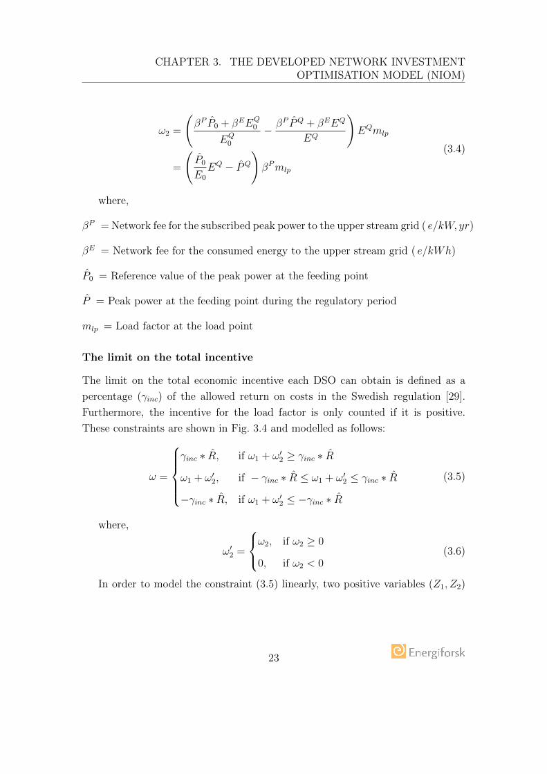
We model the network fee paid to the upper stream grid by two parts [51];

one part is related to the subscribed capacity, the other part is related to the

transported energy as shown in (3.4). The subscribed capacity is decided by the

DSO for the coming years. It is assumed that the DSO always subscribes the

capacity according to the peak power in the network. The price of the network fee

to the upper stream grid is assumed unchanged from the reference years and the

considered regulatory period. In order to model this incentive (3.3a) linearly, the

load factor at the load point is used. Modelling the load factor at the load point

is also reasonable, because the DSM devices are implemented at the load points.

The load factor at the load point and the feeding point are the same if the network

is lossless and there is no DG in the network.

22


ω2 =

(βP P0 + βEEQ

0

EQ0

− βP PQ + βEEQ

EQ

)EQmlp

=

(P0

E0

EQ − PQ

)βPmlp

(3.4)

where,

βP = Network fee for the subscribed peak power to the upper stream grid ( e/kW, yr)

βE = Network fee for the consumed energy to the upper stream grid ( e/kWh)

P0 = Reference value of the peak power at the feeding point

P = Peak power at the feeding point during the regulatory period

mlp = Load factor at the load point

The limit on the total incentive

The limit on the total economic incentive each DSO can obtain is defined as a

percentage (γinc) of the allowed return on costs in the Swedish regulation [29].

Furthermore, the incentive for the load factor is only counted if it is positive.

These constraints are shown in Fig. 3.4 and modelled as follows:

ω =

γinc ∗ R, if ω1 + ω′2 ≥ γinc ∗ R

ω1 + ω′2, if − γinc ∗ R ≤ ω1 + ω′2 ≤ γinc ∗ R

−γinc ∗ R, if ω1 + ω′2 ≤ −γinc ∗ R

(3.5)

where,

ω′2 =

ω2, if ω2 ≥ 0

0, if ω2 < 0(3.6)

In order to model the constraint (3.5) linearly, two positive variables (Z1, Z2)

23


ω1 + ω′2

ω

ω2

ω′2

Figure 3.4: The limits on the total incentive.

are introduced with a penalty in the objective function:

ω = ω1 + ω′2 (3.7a)

−γinc ∗ R ≤ ω + Z1 − Z2 ≤ γinc ∗ R (3.7b)

REG = R + ω + Z1 − Z2 (3.7c)

Z1 ≥ 0 (3.7d)

Z2 ≥ 0 (3.7e)

In order to model the constraint (3.6) linearly, a binary variable (Dpos) are

introduced.

ω′2 ≤ Dpos ∗M (3.8a)

ω′2 ≤ ω2 + (1−Dpos) ∗M (3.8b)

3.2.3 Modelling of DG curtailment

Two variations of curtailment regulation are modelled. The curtailed energy in

the system is assumed to be regulated by either the quantity-regulatory approach

or the price-regulatory approach, as introduced in Chapter 2. If it is regulated

by the quantity-regulatory approach, the cost of curtailment (Ccurt ) is based on

the curtailment that is above the pre-agreed maximum curtailment level. This

excess part is modelled by positive variables gn,cmt as shown in (3.9a). γcur is

the pre-agreed maximum curtailment level as a share of available DG. (3.9a) is

valid for each DG unit in each planning period. If it is regulated by the price-

regulatory approach, the total curtailed energy is the sum of the curtailed energy

24


in all scenarios, as shown in (3.9b).∑sc∈Nsc

Pn,curt,sc ∗ Pbsc ∗ τt − gn,cmt ≤ γcur∑

sc∈Nsc

Pnt,sc ∗ Pbsc ∗ τt n ∈ NDG (3.9a)

∑sc∈Nsc

Pn,curt,sc ∗ Pbsc ∗ τt = gn,cmt n ∈ NDG (3.9b)

where,

γcur = Maximum curtailment percentage.

P n,curt,sc = Curtailed power in planning period t and scenario sc on node n.

Pbsc = Probability of scenario sc.

τt = Time duration of planning period t.

P nt,sc = Available power in planning period t and scenario sc on node n.

gn,cmt = Curtailed energy from node n that is compensated in planning period t.

3.2.4 Modelling of DG connection and unbundling regula-

tion

In the unbundled power systems, the connection lines of DG are decided by the DG

owners instead of the DSOs. In the deep connection fee regime, it is assumed that

DG owners choose connection lines which have the least price offered by DSOs and

that DSOs offer a price which is equal to the cost. Therefore, in this case the lines

to connect DG are determined by the cost for DSOs or the profit of DSOs. The

connection lines are then determined by the network investment model. However,

in the shallow connection fee regime, DG owners choose connection lines from

their own interest. Modelling DG owners’ interest is outside the scope. Therefore,

the connection lines are treated as given parameters. This enables the model to

minimise reinforcement cost on the network given the connection lines that DG

owners propose.

3.2.5 A summary of the models

A summary of modelling these four kinds of regulation is presented in Table 3.1.

In reality each power system is under a combination of regulations.

25


Table 3.1: A summary of modelled regulations

Regulatory issues Modelling

Revenue cap regulation (3.1)

Performance regulation

– lossesReward and penalty (3.2)


– load factorsReward only (3.4) (3.8)


– the totalLimited incentive (3.7)

Curtailment regulationQuantity-regulatory (3.9a)

Price-regulatory (3.9b)

DG connections/unbundlingDeep

DG connection lines

as output

ShallowDG connection lines

as input

3.3 Formulation of the developed NIOM

The distribution network infrastructure investment is modelled as a two-stage

decision making optimisation problem with recourse. The first stage investment

decisions are made under uncertainties of load and DG. When the uncertainty is

disclosed, the second stage decisions are taken. The investment model presented

here considers essential network constraints such as voltage, thermal limits and

power balance. It is compatible with the economic constraints from economic

regulation as presented in Section 3.2. Some constraints are modelled as linear

constraints according to the algorithm which is applied to solve it.

3.3.1 Variables

The investment decisions considered in the model are the new DG connection

routes and conductors of the connection lines (Dl,alt , al ∈ AL, l ∈ Kdg), substa-

tions updates (Dn,alt , al ∈ AL, n ∈ Ns) and reinforcements in the existing lines

(Dl,alt , al ∈ AL, l ∈ L). Note that the timing of these decisions are also con-

sidered. These variables are made under uncertainties of load and DG, which are

26


0

8

5

1

planning

period(t)

first stage

decision

(Dl,alt , Dn,al

t )

second stage

decision

(P n,cur1,1 , . . . , P cur

4,n )

0 1 2 3 4

D1 D2 D3

9

12

16

17

20

24

25

28

32

1

sc = 1

...

sc = n

Figure 3.5: Scenario fan within the perspective of decision framework.

referred to as the first stage decision variables in a two-stage stochastic optimisa-

tion problem. The relations between the stage and the variables are illustrated in

Fig. 3.5.

When the uncertainty is disclosed, which can be any scenario (sc) from 1-n

in Fig. 3.5, the second stage decisions are taken. In this model, the second stage

decision variables are the timing and amount of DG curtailment(P curt,sc ). Load

shedding is modelled but assumed not to be allowed. These decisions depend on

the current in each line and voltage in each node, which are also determined when

the uncertain load and DG production are realized.

3.3.2 Objective function

Two objective functions are modelled. One is to minimise the net present value

(NPV) of the total expense in the network as shown in (3.10). The total expense

is the sum of the expense for the network infrastructure and network operation.

Cost minimisation is an ideal case. The solution from it can serve as a reference

value. The other one is to maximise the NPV of the total profit for the DSO in

a regulatory period as shown in (3.11). The profit is the revenue minus the cost.

The revenue is limited by a revenue cap. The solution from profit maximisation is

assumed to be a rational DSO’s decision under incentive regulations.

27


The capital expenditure (Ccapt ) is determined at the beginning of the planning

horizon and is for the investment of replacement of or updating the existing lines or

substations and installation of new lines. Whether the cost of the connection lines

for DG is included in the capital expenditure depends on the connection charge

regulation, as explained in Section 3.2.4. The connection line cost is included in the

case of deep connection charge, and it is excluded in the case of shallow connection

charge. The expenses for operation in (Copert ) is considered at the beginning of each

planning period. It corresponds to the cost of losses and DG curtailment during

this planning period. However, whether and how the cost of losses and curtailment

are included in the operational expense depends on the economic regulation, as

explained in Section 3.2.3.

min NPV

(T∑t=1

(Ccapt + Copert )

)(3.10)

max NPV

(T∑t=1

(Rt − (Ccapt + Copert ))

)(3.11)

where,

Ccapt =∑l∈R

∑al∈AL

CR,ALl,al Dl,alt +

∑l∈K

∑al∈AL

CK,ALl,al Dl,alt +

∑n∈Ns

∑al∈AL

Cn,alDn,alt (3.12a)

Copert = C losst + Ccurt (3.12b)

C losst =∑

sc∈Nsc

P losst,sc ∗ λloss ∗ Pbt,sc ∗ τt (3.12c)

Ccurt =∑

n∈NDG

gn,cmt ∗ λcur (3.12d)

3.3.3 Technical constraints

Power balance at each node, Kirchhoff’s current law (KCL), Kirchhoff’s voltage

law (KVL), voltage and thermal limits and logical limits are constraints considered

in this model. Most of the constraints are similar to constraints in a conventional

network planning model such as the one in [39]. The modified parts compared

to [39] are that: (i) correlated load and DG scenarios are considered, (ii) AC

power flow equations are used instead of DC power flow equations, and (iii) DG

production and location are not optimised by the DSO.

28


The technical constraints for the network investment model are shown as fol-

lows.

1. power balance

f(V nre,t,sc, V

nim,t,sc, I

nre,t,sc, I

nim,t,sc) = (Pnt,sc−P

n,curt,sc )+j∗(Qnt,sc−Q

n,curt,sc ) for n ∈ N

(3.13)

2. KCL and KVL

AILre,t,sc = INre,t,sc, I lre,t,sc =∑al∈AL

I l,alre,t,sc l ∈ L (3.14a)

AILim,t,sc = INim,t,sc, I lim,t,sc =∑al∈AL

I l,alim,t,sc l ∈ L (3.14b)

(A>lVNre,t,sc)E

l,al − (Rl,alI l,alre,t,cs −X l,alI l,alim,t,sc)El,al = 0 l ∈ L, al ∈ AL (3.14c)

(A>lVNim,t,sc)E

l,al − (Rl,alI l,alim,t,cs +X l,alI l,alre,t,sc)El,al = 0 l ∈ L, al ∈ AL (3.14d)

3. losses

(V NSt,sc I

NSt,sc)re +

∑n∈NDG

Pnt,sc −∑

n∈NDG

Pn,curt,sc −∑

n∈NLD

Pnt,sc = P losst,sc (3.15)

4. physical limits

|V Nt,sc| ≤ V N

max (3.16a)

V Nmin ≤ |V N

t,sc| (3.16b)

|I l,alt,sc| ≤ I l,almaxEl,al l ∈ L, and |INS

t,sc| ≤ INSmaxE

NS ,al (3.16c)

Pn,curt,sc ≤ Pnt,sc, n ∈ NDG (3.17a)

Qn,curt,sc ≤ Qnt,sc, n ∈ NDG (3.17b)

5. logical constraints∑t∈T

∑al∈AL

Dl,alt ≤ 1 l ∈ R ∪K, (3.18a)

El,alt ≤ El,alt−1 +Dl,alt l ∈ R ∪K, al ∈ AL (3.18b)∑

al∈ALEl,alt = 1 l ∈ R ∪K (3.18c)∑

al∈ALEl,alt ≤ 1 l ∈ Kdg, dg ∈ NDG (3.18d)∑

t∈T

∑al∈al

El,ALt ≥ 1 l ∈ Kdg, , dg ∈ NDG (3.18e)

29


Constraint (3.13) represents the power balance in each node. It is approximated

by the first order Taylor expansion as shown in (3.19-3.20b). The expansion is

evaluated at a starting point in the first iteration. If the iteration continues, it

is re-evaluated at the previous operation point. They are shown in (3.20a) and

(3.20b) respectively, where the subscription t and sc are not shown for readability.

fp(Vnre, V

nim, I

nre, I

nim, V

n,dre , V n,d

im , In,dre , In,dim ) = Pn − Pn,cur

fq(Vnre, V

nim, I

nre, I

nim, V

n,dre , V n,d

im , In,dre , In,dim ) = Qn −Qn,cur

n ∈ N, d = h− 1

(3.19)

fp = V n,dre Inre + V n,d

im Inim + V nreI

n,dre + V n

imIn,dim − (V n,d

re In,dre + V n,dim In,dim ) (3.20a)

fq = V n,dim Inre − V n,d

re Inim − V nreI

n,dim + V n

imIn,dre − (V n,d

im In,dre − V n,dre In,dim ) (3.20b)

Constraints (3.14a-3.14b) represent the Kirchhoff’s current law (KCL). Con-

straints (3.14c-3.14d) represent the Kirchhoff’s voltage law (KVL). Constraints

(3.14c-3.14d) are valid if a line exists between two nodes. A big number M is

added to make sure that only if the line does exist, there is an equality constraint

that represents KVL, as shown in (3.21a-3.21b).

(A>lVNre,t,sc)−Rl,alI l,alre,t,cs +X l,alI l,alim,t,sc ≤M(1− El,al) (3.21a)

(A>lVNim,t,sc)−Rl,alI l,alim,t,cs −X l,alI l,alre,t,sc ≤M(1− El,al) (3.21b)

Equality constraint (3.15) calculates the thermal losses in the system. This is

the difference between the injected energy and the consumed energy. The thermal

loss is an important variable since it can be linked with the incentive performance

regulation. It is also part of the operational cost that used in the reference case

where the total cost is minimised. Constraint (3.17) ensures that the curtailment

is not more than the DG production.

Constraints from (3.18a) to (3.18e) show the logical constraints for the invest-

ment and availability of each branch and alternatives. Equation (3.18a) shows

that maximum one investment on each branch (and substation) is permitted in

the planning horizon. Equation (3.18b) shows that the alternatives for replacement

30


or connection branches (and substation) are available only after the corresponding

investment has been done. Equation (3.18c) shows that only one alternative of

replacement branches will be available in a period. Equation (3.18d) shows that

at most one branch among the connection branches is built to connect DG in one

period. Equation (3.18e) shows that all DG should be connected in the end of the

planning period.

Formulate and solve MILP subproblem:

Obj. (5.10) or (5.11) s.t. constraints of economic regulation;linearized technical constraints (5.14a-

b, 5.15, 5.17a-5.18e, 5.20a-5.28b).

Optimal Solution

Initialization (5.13)

Stopping criteria

Update the linearized constraints (5.20a-b, 5.25-5.28b)

h=0

h=h+1

No

Yes

Formulate the network investment model

Obj. (5.10) or (5.11)

s.t. incentive regulation(5.1-5.2, 5.4, 5.7-5.8)curtailment regulation(5.9a, 5.9b) technical constraints(5.13-5.18e)

Figure 3.6: Outline of the solution method for NIOM.

3.4 Modelling of reliability

Reliability indices, expected energy not served (EENS), system average interrup-

tion duration index (SAIDI) and system average interruption frequency index

(SAIFI) are calculated for the obtained systems. Since reliability requirements

are not modelled explicitly in the optimization model, the optimal solution may

be less desirable when the cost of reliability is considered. Therefore, a solution

pool with several best solutions in the optimization are saved to further study the

system reliability.

The switching devices in the system which are used for preventing the extension

of failure in the system and maintenances, are not modelled and therefore the reli-

31


ability is evaluated through a compromise solution between an upper and a lower

bound on the reliability level. The upper bound is calculated assuming that no

switching devices are installed in the network, while the lower bound is calculated

assuming that all branches are equipped with switching devices. The compromise

is modelled by an improvement coefficient [52]. It is a coefficient to simulate the

effect of a compromise solution in switching device location. The reliability level

is estimated by an analytical method considering all line failures, one at a time,

and load levels [53, 40]. DG units are considered as alternative supplying sources

when an outage occurs [53]. The simulation steps are summarized as:

1. Select a solution file from the pool.

2. Obtain the network configuration in a planning period.

3. Select a load/DG scenario and a failure event.

4. Evaluate the upper bound and lower bound of reliability indices given the

failure rate and restoration time.

5. Repeat step 3-4 for all scenarios and all failure events in the planning period.

The expected value for those indices are calculated per period.

6. Repeat 2-5 for all planning periods. An improvement coefficient is defined

to calculate the estimated reliability indices.

7. Repeat 1-6 for all solutions

32

Chapter 4

The developed network

investment assessment model

(NIAM)

4.1 Modelling of line capacity

A general DLR calculation model is developed based on the standard line capacity

calculation. It is simplified and easy to be implemented.

4.1.1 Standard line capacity calculation

IEEE standard 738 [54] gives a standard formula for calculating the current of

bare overhead conductors. It is based on steady-state heat balance:

I =

√qc + qr − qs

Rc

(4.1)

where qc is the convective cooling, qr is the radiative cooling, and qs is the solar

heating. Rc is the resistance of the conductor at temperature Tc. Solar radia-

tion is neglected and the variation of resistance is neglected for the line capacity

calculation in this paper. The line capacity can be calculated as below [54]:

IDLRmax ≈ max (4.2)

33

CHAPTER 4. THE DEVELOPED NETWORK INVESTMENTASSESSMENT MODEL (NIAM)

√[1.01 + 0.0371 ∗ (

D∗ρf∗vµf

)0.52] ∗ [kf ∗Kangle ∗∆T ]√Rc

;√[0.0119(

D∗ρf∗vµf

)0.6] ∗ [kf ∗Kangle ∗∆T ]√Rc

where ∆T = Tc − Ta. D is the conductor diameter, ρf is the density of air at

temperature Tf (Tf = Tc+Ta2

, where Tc and Ta are conductor temperature and

ambient air temperature respectively), v is the speed of air stream at conductor,

µf is the dynamic viscosity of air at temperature Tf , kf is the wind direction

factor at temperature Tf , Kangle is the parameter represents the angle between

wind speed and the conductor axis. The formula above corresponds to low wind

speeds, while the one below corresponds to high wind speeds. However at any

wind speed, the larger of the two value is used [54].

The line capacity in reality is varying with many parameters as shown in (4.2),

however, it is useful to simplify it to be easily implemented for electric power

system planning and operation. In general, there are two ways to simplify the

capacity calculation, SLR and DLR.

4.1.2 Calculation of static line rating (SLR)

SLR needs the parameters from a scenario, which usually is the worst scenario

considering the worst possible conductor temperature, the ambient air tempera-

ture and the wind speed. For example, Engineering Recommendation (ER) P27

[55] proposes to calculate seasonal thermal ratings using assumed temperatures

for different seasons and for a constant wind speed of 0.5 m/s and zero solar radi-

ation [56]. The conventional relations between Tf , µf , ρf and kf can be found in

Standard 738 [54].

ISLRmax = (4.3)√[1.01 + 0.0371 ∗ (

D∗ρf∗vSLR

µf)0.52] ∗ [kf ∗Kangle ∗∆T SLR]

√RSLR

where vSLR is the wind speed, ∆T SLR is the temperature difference, RSLR is the line

resistance in the worst scenario. Other parameters depends on Tf also correspond

to the worst scenario.

34


4.1.3 Calculation of dynamic line rating (DLR)

DLR estimates the line ampacity in real time with monitored weather conditions

taking account of the wind cooling effect [57]. It can be obtained using a variety

of methods: conductor sag and tension monitoring, vibration mode analysis, con-

ductor temperature and local weather data [58] [57]. Temperature and wind speed

are the parameters that affect DLR significantly, furthermore, the higher the wind

speed, the higher the wind power production and (simultaneous) transfer capacity.

As for the correlation between temperature and the wind speed are unclear, their

impact on capacity ratio are studied separately. Here a simplified DLR calcula-

tion model is developed based on the assumption that wind impact on the line

rating and temperature impact on that are independent. This is demonstrated as

a reasonable assumption in Paper IV.

The proposed DLR model is based on the the capacity ratio between DLR

and SLR. This ratio (η) is a function of wind speed and temperature, as shown

in (4.4) . The variation of resistance due to temperature is neglected for the line

capacity calculation in this paper. Under the independence assumption, ηv and ηT

are obtained separately.

η(v, T ) =IDLRmax

ISLRmax

≈ ηv ∗ ηT (4.4)

where ηv is the ratio related to the wind speed, and ηT is the ratio related to

the relevant temperature values. Given the same temperature for DLR and SLR

calculation, all the temperature related parameters (ρf , µf , kf and ∆T ) are the

same for both cases. We also use the wind speed v that is perpendicular to the

conductor, so the wind direction factor Kangle is equal to 1. The parameters to

define ηv can be estimated for both low wind speed (ηlow(v)) and high wind speed

(ηhigh(v)). Note that even the wind speed is very low, the line rating ratio should

not be lower than 1.

ηv = max (4.5)

35


1;

ηlow(v) ≈ 1

v0.26SLR

∗ v0.26 = α ∗ v0.26;

ηhigh(v) ≈ 0.566

v0.26SLR

(ρfµf

)0.04D0.04v0.3 = β ∗D0.04 ∗ v0.3.

where α = v−0.26SLR and β = 0.559v0.26SLR

(ρfµf

)0.04. Conventional vSLR = 0.5, then α ≈ 1.1975.

If we further assume that some of the temperature related parameters, ρf , µf

and kf , are the same in the DLR and SLR calculation. Therefore, the value of β

is set by the Tf in SLR calculation. η(v, T ) is derived as:

η(v, T ) = max (4.6)

1;

≈ ηlow(v)

√Tc − TaTc − T SLRa

= ηlow(v)ηT ;

≈ ηhigh(v)

√Tc − TaTc − T SLRa

= ηlow(v)ηT .

where ηT can be expressed as:

ηT ≈

√Tc − TATc − T SLRa

= γ∆T 0.5 (4.7)

where γ =√

1Tc−TSLR

aand ∆T = Tc − Ta

4.2 Formulation of the developed NIAM

This developed NIAM applies the developed DLR calculation model to analyse

impact from DLR on wind power integration. The main inputs for the analysis

are the wind speed and the ambient temperature. Two outputs produced from

the analysis are investment in wind power connection and curtailed wind power,

which can be used for the decision-making in power distribution. The model is

based on life cycle cost analysis (LCCA). Life cycle cost (LCC) is the annualized

cost of an investment during its entire economic lifetime. LCCA often includes

costs of investments, outages, maintenance, interests and incomes (modelled as

negative costs) [59]. The estimated lifetime is limited by the technical lifetime,

36


technical developments and expansions in power distribution systems [59]. The

LCCA without considering the incomes is performed as follows in each simulation.

LCCinv = Capex+LT∑i=1

Opexiqi− R

qLT(4.8)

q = 1 +z

100(4.9)

The flow chart of the algorithm is shown in Fig 4.1. First, as shown in Box a, the

Start first simulation: s=1

Set: the number of simulation N, maximum number of wind power plants NP,

Economic life time LT,The number of periods in a year K

- Generate wind power production if no transfer limitations are considered - Calculate transfer limitations:

Begin calculation regarding year 1 : i=1

Obtain the weather parameters and wind speed at hour 1: k=1

i ≤ LTk ≤ K n ≤ NP s ≤ N

Results

- Calculate LCC for each investment alternative- Calculate DisENS for each investment alternative

No No No

No

s = s + 1

n= n

+ 1

i = i + 1

k = k + 1

Yes

Yes

Yes

max max , ,,DLR SLR

s i kI I

, , ,s n i kP

, , ,s n i kDiscENSx

Yes

Box a

Box b

Box c

, , ,s n i kLCCx

Figure 4.1: Model for assessing wind power connection using SLR and DLR.

number of simulations(S), the maximum number of wind power plants (NP), the

economic life time of the power plants (LT) and the number of periods in a year

(K) are set. A common way to divide the year is into months, i.e. K = 12. Hence,

there are S ∗ LT ∗ K generations of stochastic variables for a certain number of

WP plants.

37


Then, as shown in Box b, stochastic (temperature and wind power production)

inputs are generated in each simulation. To save time without losing any generality,

the same stochastic variables are used for calculation regarding different numbers

of wind power plants. In this model, wind power production is assumed to be

correlated only to wind speed and not to temperature. By comparing the generated

wind power and the line limits, the permissive transferred power is obtained.

The income from transferred power is considered as negative costs. It is dis-

counted to the net present value (NPV). Therefore the LCC for the investment,

Box c, is calculated as in (4.10-4.14).

Incs,n,i,k = min(Ps,n,i,k, Ps,n,i,k) ∗ Eprice (4.10)

Ps,i,k = Is,i,k ∗ UN (4.11)

Is,i,k ∈ {IDLRmax , ISLRmax }s,i,k (4.12)

LCCs,n,i,k = LCCxinv − 1

(1 + z)i∗ Incs,n,i,k (4.13)

LCCs,n = LCCxinv −LT∑i=1

1

(1 + z)i

12∑k=1

Incs,i,k (4.14)

where k represents any period in a year, i represents any year during LT, n denotes

the number of the wind farms, s presents any simulation. Ps,i,k is the maximum allowed

power on the connection line, which is calculated by the maximum line capacity and

nominal voltage at the connection point of wind power plants. x represents different

investment alternatives. If the average LCC is negative at the end of the economic

lifetime, this indicates that the investment is profitable.

The amount of disconnected energy (DiscENS) is recorded in each simulation, as

shown in Box c, if it is applicable. It reflects the utilisation of the network and the

renewable energy. It is assumed that the DSO can disconnect the wind power plants

or ask wind power plant owners to reduce the production. The exported wind power is

limited by the line rating, so when wind power plants produce more than the limit, the

extra energy will be curtailed. In the model, the production of the wind power plants

is first generated without considering the transmission limits, then the sum of curtailed

power is calculated according to the limits. Therefore, the curtailed energy is modelled

by DiscENS.

DiscENSs,n,i,k = max(Ps,n,i,k, Ps,n,i,k)− Ps,n,i,k (4.15)

Although costs of introducing DLR are not considered in this simulation model.

38


However, by calculating the difference in profit between SLR and DLR, it reveals the

benchmarking cost for introducing DLR.

39

Chapter 5

Application of developed models

5.1 Application of NIOM

To apply the proposed NIOM, a radial network with 21 load nodes and two DG plants

which have asked for connection is created. The type and size of the DG are not decided

by the DSO due to the unbundling regulation. The distribution network is displayed in

Fig. 5.1. It operates at 24.9 kV. Two wind farms are in the pipeline to be connected. In

the figure, the square node represents the feeding substation, the wind turbines represent

wind farms, and the circles are the load points and wind farm locations (N22 and N23).

Continuous lines denote the existing network and dashed lines are candidate routes for

new connections. The system details (node data and line data) can be found in [60].

Investment for one regulatory period of four years is considered in the case study. A

DG owner applies for a connection to N22 in year 2 and another DG owner applies for a

connection to N23 in year 3. The installed capacity of DG accounts for 47% of the total

load. In this grid, all lines have two alternatives for upgrade, AL1 is the initial line and

AL2, AL3 are the alternatives to upgrade. There are three paths to connect each new

wind farm into the network. L8, L13, and L21 are for N22. L9, L15, and L24 are for

N23. Each new path has three alternatives.

5.1.1 Case study for incentive regulation

This application looks into the DSOs’ investment decisions and performances under the

Swedish distribution network regulation, which is a revenue cap frame with performance

incentives. In the application, the input load profiles are with three different load factors

(mlp) but the same total yearly energy consumption at each load point. Load shedding

40

CHAPTER 5. APPLICATION OF DEVELOPED MODELS

1 2 3 4 5

6

7

8 9 10 11

12 13 14 15

16 1817

19 20

21L1

L8 L7

L13

L12

L3

L18 L19 L22

L26

L5

L4L2

L6 L11

L10

L23 L25

L17L16L14

L15L24

L9

L20

L21

23

22

Figure 5.1: Diagram of the 23-node network.

is assumed to be not allowed. DG owners pay a fee based on deep connection cost

and their curtailment is compensated by the electricity price. The network infrastruc-

ture investment cost is calculated for two situations, with DG and without DG. DSOs’

investment decision is based on maximizing the total profit within the regulatory frame-

work. Furthermore, the decisions based on minimizing the total cost are presented as

a comparison. Ideally, the DSO opts for the decisions resulting the least total costs

considering both operational cost and capital cost.

Benchmark price for load factor increase

The total profit of the DSO increases with the increase of mlp value in both with and

without DG cases. By comparing profits between different mlp values, the benchmark

price to invest in increasing mlp values is obtained. If the investment to increase mlp is

lower than the benchmark price, it is profitable to invest in increasing mlp. For example,

the benchmark price to increase mlp from 0.5 to 0.6 is 84.31× 105 e, and the benchmark

price to increase mlp from 0.6 to 0.7 is 122.20 × 105 e if there is DG in the system.

By comparing these two benchmark prices, the incentive to increase load factor from

medium to high is higher than from low to medium in the system with DG. In the

systems where there is no DG, the benchmark price to increase mlp from 0.5 to 0.6 is

227.37×105 e, and the benchmark price to increase mlp from 0.6 to 0.7 is 119.51×105 e.

By comparing these two benchmark prices, the incentive to increase load factor from low

to medium is higher than from medium to high in the system with DG. Furthermore,

the economic incentive for the DSO to invest in increasing the load factor, for example

through ANM, are high, accounting for more than 18% of the profits, in systems with

41


or without DG. With the same m value, the profit is higher in the system with DG than

without DG. However, the profit in the system with DG is over-estimated because the

allowed return on costs is assumed to be the same as in the system without DG. The

potential deferral of network investment due to the DG connection is not considered in

the regulation.

Benchmark price for loss reduction

By implementing different incentive regulations, the infrastructure investment costs and

profits of the DSO are obtained by the developed model. The infrastructure investment

costs do not vary nor do the operational costs, but the total profits do. This means that

the economic incentive in loss reduction is not high enough to change the infrastructure

investment decisions.

The reward for reducing losses in kWh can be estimated for a given network. The

reward is measured by the increased revenue cap due to the loss reduction. In this

example, comparing the case with and without the incentive for loss reduction, the gain

due to loss reduction is 7.37 × 105 e in the case with DG and and 6.72 × 105 e in the

case without DG. The reward/penalty price for loss reduction/increase, which is the

incentive ω1 divided by the reduced losses in kWh, is 0.053 e/kWh in this case for the

system with DG. It is 0.001 e/kWh higher than the expected electricity price. The

reward/penalty price for loss reduction/increase is 0.048 e/kWh in this case for the

system without DG, which is 0.004 e/kWh lower than the expected electricity price.

These prices can be used as a benchmark to evaluate the cost to reduce losses.

Discussion

In this application, we studied the performance of the different incentive regulatory

regimes for distribution network investment with and without DG. We found that the

incentive for load factor increase does impact on the network infrastructure investment,

but the incentive for loss reduction does not. With the increase of load factor, less

network infrastructure cost is observed. We also estimated the benchmark prices for

investing in increasing load factor and decreasing losses in the Swedish regulation frame-

work by the proposed method. This approach can also be applied in other regulation

frameworks by adjusting the regulatory constraints and parameters. These benchmark

prices can be used to evaluate the feasibility of investing in improving performance in-

dices. They can also be used by regulators to evaluate the impact of the performance

incentives. We observed in this case study that although the total performance incentive

42


is lower in the system with DG than without DG, the total profit is higher. For detailed

results and analysis, please refer to Publication II.

5.1.2 Case study for curtailment regulation

Quantity-regulatory approach

In this case study, the quantity-regulatory approach for curtailment is investigated. Each

DG owner is compensated for the annual curtailed energy which is above a predefined

level. This level is referred to as non-compensated level in this case study. The non-

compensated level is 3% per year for each DG unit. The production is remunerated by

feed-in tariff (FiT) (0.13 e/kWh) and is compensated by the same price if the production

is curtailed. Different non-compensated levels are applied, and different compensation

prices are discussed in this case study.

DG owners pay for the shallow connection charge; therefore, the connection lines are

decided from the DG owners’ interest not considering the reinforcement of the rest of

the grid. In this application, we assume that L13 AL2 T2 (AL 2 of the line L13 is built

at year 2) and L24 AL1 T3 (AL 1 of the line L24 is built at year 3) are chosen by the

DG owners. The DSO minimising Ctotal as in (3.10) with constraints (3.13-3.18), (3.9a),

where λcur = λDGel and two DG connections are given.

The results for applying the quantity-regulatory approach are presented in Table

5.1. It shows that the higher the non-compensated curtailment level is, the lower the

total expected cost and the higher the optimal curtailment levels. Moreover, allowing

a lower non-compensated annual curtailment level does not lead to more reinforcement

for the network, since paying for curtailing energy in some years is more beneficial than

reinforcing the network. The higher the curtailment is the lower the thermal loss is;

however, the impact is small.

In order to investigate the relation between the network investment and the non-

compensated curtailment level, the optimal network investment with different maximum

annual curtailment levels are simulated without compensation. The simulation starts

from the curtailment level 3% since the connection lines for DG are chosen based on

accepting this curtailment level. In Fig. 5.2, the optimal solutions are based on minimis-

ing Ctotal =∑T

t=1(δcapt Ccapt ) in (3.10) with constraints (3.13)-(3.18) and (3.9a), where

gNDG,cm

t = 0 and changing γ from 3% to 50%. The avoided network reinforcement cost

is the difference between the minimum capex when γ is 3% and when γ is higher. The

avoided capex increases as the maximum annual DG curtailment level increases. Due

to the nature of integer optimisation, the increase is stepwise. The increase stops when

43


Table 5.1: Results for the case under quantity-regulatory approach

γ 3% 15%

λcur(e/kWh) 0.13 0.13

Total cost(ke) 590.450 580.712

Capex(ke) 472.405 472.405

Connection cost(ke) 37.33 37.33

Compensation (N22,N23)(ke) 9.40, 0 0, 0

Curtailment percentage (N22,N23) 5.3%, 3% 15%, 0%

Loss percentage 2.83% 2.82%

the maximum annual DG curtailment level is 8%.

By adjusting the non-compensated curtailment level, the benefit for the DSO in-

creases while the value of curtailed energy remains the same. The value of curtailed

energy is related to its opportunity cost. In this case, the opportunity cost is evalu-

ated by the FiT for renewable energy. Furthermore, by increasing the FiT, the distance

between the avoided total cost and value of curtailed energy can change, and therefore

the benefit for the DSO can change. In this case when the FiT increases by five times,

the value of allowing curtailment decreases and the maximum benefit for the DSO is

reached when the maximum annual curtailment level is between 4% and 5%, as shown

in Fig. 5.3.

Price-regulatory approach

In this case study, the price-regulatory approach for curtailment is investigated. If the

compensation price is the same as or higher than the electricity price for DG, the DG

owners lack incentives to increase the penetration level of distributed energy. Therefore,

the curtailed energy is suggested to be compensated with a price that is less than the

price to sell the same quantity of energy [20].

In this case, the DG owner chooses connection points considering necessary net-

work reinforcement since the DG owner pays for the reinforcement and possible energy

curtailment. The connection decision is based on maximising the DG owner’s benefit,

which is ((gNDG,tot − gNDG,cur) ∗ λDGel + gNDG,cur ∗ λcm − Cnetwork). where Cnetwork is

the network cost due to the DG connection. Given λcm is less than λDGel in the price-

regulatory approach and λDGel is exogenous, the decision will be based on minimising

Cnetwork which is Ctotal as in (3.10) where Copert = Ccurt and λcur = λDGel − λcm, with

44


5 · 10−2 0.1 0.15 0.2 0.25 0.3 0.35 0.4 0.45 0.5−20

0

20

40

60

80

100

Max. annual curtailment level (100/%)

Cos

ts/V

alue

(k)

Avoided capexValue of curtailed energyCompensation for curtailed energyValue of allowing curtailmentBenefit for the DSOAvoided cost of losses

Figure 5.2: FiT is 0.13 e/kWh.

constraints (3.13)-(3.18) and (3.9b).

Table 5.2 presents the results in this case. By increasing the price, the capex decreases

stepwise. Table 5.2 shows the three steps observed in this case. With the increase of

the compensation price, the total curtailment increases. Furthermore, with the increase

of the compensation price, the network investment decreases but the connection cost

may increase. Comparing the case where the compensation price is 0.08 e/kWh with

0.026 e/kWh, the curtailment level is higher and the connection cost is also higher.

This is because when the connection line is L21, reinforcement on L3 is necessary and

the cost to reinforce L3 is high. However, when the connection line is L13 AL2, although

it is more expensive than L21 AL1, curtailment in the planning periods makes that the

reinforcement on L3 is no longer necessary. On the other hand, the curtailment in the

case with compensation price 0.11 e /kWh is higher than the case with compensation

price 0.08 e/kWh, and the connection cost is lower. This is because the compensation

price is so high that it is not worth reinforcing the network and investing in a larger

capacity of the connection line from the DG owners’ perspective.

By allowing different annual curtailment levels in the same network, the minimum

capex and the optimal curtailment are simulated. The avoided capex, avoided cost of

45


5 · 10−2 0.1 0.15 0.2 0.25 0.3 0.35 0.4 0.45 0.5−100

−50

0

50

100

150

200


Cos

ts/V

alue

(k)e

Avoided total costValue of curtailed energyCompensation for curtailed energyValue of allowing curtailmentBenefit for the DSO

Figure 5.3: FiT is 0.65 e/kWh.

losses, and the value of curtailed energy are plotted, as shown in Fig. 5.4. It shows that

the value of curtailed energy is always higher than the avoided total cost. The benefit

of the DG owner is the difference between the avoided capex and the economic loss due

to the low compensation price for curtailed energy. The economic loss is the value of

the curtailed energy minus the compensation for it. It is better to curtail some energy

for the DG owner when the compensation price is higher, and vice versa as shown in

Fig. 5.5. The maximum benefit is 8.89 ke when the compensation price is 0.11 e/kWh,

while the the maximum benefit is 0 when the compensation price is 0.026 e/kWh.

Discussion

The non-compensated curtailment level in the quantity-regulatory approach for energy

curtailment due to network constraints can affect the benefit for the DSO but not the

optimal investment. Therefore, this level is used to share the cost between the DSO

and the DG owners. The compensation price can affect the optimal investment for the

DSO. Using the quantitative model, the compensation price which changes the optimal

investment can be identified, in this case, the optimal investment for the DSO changes

46


Table 5.2: Results for the case under price-regulatory approach

λcm(e/kWh) 0.026 0.08 0.11

Total cost(ke) 481.487 480.980 472.596

Capex (ke) 481.487 472.405 461.757

Curtailment(%) (N22,N23) 0%, 0% 5.4%, 0% 16.8%, 0%

Connection lines L21 AL1 T2 L13 AL2 T2 L13 AL1 T2

L24 AL1 T3 L24 AL1 T3 L24 AL1 T3

Connection cost (ke) 28.53 37.33 26.68

0 5 · 10−2 0.1 0.15 0.2 0.25 0.3 0.35 0.4 0.45 0.5−20

0

20

40

60

80

100


Cos

ts/v

alue

(k)e

Avoided capexAvoided cost of lossesValue of curtailed energyCompensation (λcm = 0.11 e/kWh)Compensation (λcm = 0.026 e/kWh)

Figure 5.4: Avoided cost/value vs. Max. curtailment level.

47


0 5 · 10−2 0.1 0.15 0.2 0.25 0.3 0.35 0.4 0.45 0.5−20

−10

0

10

20


Ben

efit

for

the

DG

owner

(k)e

λcm = 0.11 e/kWhλcm = 0.026 e/kWh

Figure 5.5: Benefits for the DG owners with different compensations.

when the compensation price is five times higher.

The compensation price in the price-regulatory approach for energy curtailment

due to network constraints impacts the optimal network investment. When the price

increases, the network investment decreases but not necessarily the connection cost.

Furthermore, the compensation price indirectly drives the network reinforcement. In

this case, when the compensation price is higher than 0.08 e/kWh and lower than

0.13 e/kWh (which is the electricity price for DG), two levels of network reinforcement

are observed.

Comparing the avoided total cost in both cases, the avoided total cost is much lower

in the case under the price-regulatory approach. This confirms that the deep connection

charge gives locational incentives for the DG connection. Therefore, the DG connects

to the points which causes less reinforcement in the network. The network cost is more

sensitive to the compensation price in the case under the price-regulatory approach than

that under the quantity-regulatory approach.

The value of curtailed energy is the total value over the planning horizon; however,

the avoided total cost is the NPV of the investment. During the lifetime of the invest-

ment, curtailed energy is higher than is calculated here. Therefore, the value of curtailed

energy is under-estimated and the value of allowing curtailment is over-estimated here.

48


For detailed results and analysis, please refer to Publication I.

5.2 Application of NIAM

The developed NIAM is applied on a remote windy area in Sweden, where a wind farm

has been connected to the distribution network. More wind power (WP) plants can be

installed in that area since the connection line has been built and the windy area can

host more wind turbines. This model is able to identify the optimal number of WP

plants in the network for applying SLR and DLR, and the level of utilization of the

network in terms of the curtailed wind power. In addition, results from three kinds of

DLR models are compared to show the advantages of the proposed DLR model.

In this example, the profits of installing another 1 to 7 wind power plants are inves-

tigated and stochastic variables are generated monthly. The DSO is obliged to connect

customers (consumers and producers). However, the producer will pay for the invest-

ments needed for the connection (deep connection fee). Hence, it is necessary for WP

owners to perform cost analysis on the possible ways to connect WP plants: whether to

build a new line, or to apply DLR on the connection lines. On the one hand, extending

the capacity of the lines (building one extra line) can be challenging in a reasonable time

frame and budget and to refuse the connection of new wind farms is not an option. In

some areas, it is increasingly difficult to build additional lines or even physical upgrading

the old lines. On the other hand, DLR calculation is rather complex. And the difficulty

is to make all power system players agree on and allow the risks.

In this case study it is found that if the wind speed is less than 1.34 m/s it is

considered as low wind speed, i.e. when the wind speed is lower than 1.34 m/s, it is

always applicable to use the low wind speed formula in (4.2), and when the wind speed

is higher than 1.34 m/s, it is always applicable to use the high wind speed formula in

(4.2).

The studied investment alternatives using the SLR model are named SLR 1, which

applies SLR on the existing network to identify the network transmission limit, and SLR

2, which is to build an extra connection line in order to increase the transmission limit.

Two variants of the proposed DLR calculation model presented in section 4 are also

implemented as investment alternatives: i ) a simplified version referred to as DLR 1

when only the temperature impact on line rating is considered as in (4.7), ii ) a simplified

version referred to as DLR 2 when only the wind impact on line rating is considered

as in (4.5), and iii ) the proposed DLR model is referred to as DLR 3 which takes the

temperature and wind speed impact on line rating into consideration as in (4.6). These

49


five alternatives are compared to show the value of a complex DLR model considering

both wind speed and temperature impact.

5.2.1 Case study for evaluating investment in DLR

Four aspects of five investment alternatives are analysed. First the different profits by

different alternatives with an increase of the number of wind power plants are presented.

Then the DiscENS values are compared with the increase of wind power plants. After

that the optimal wind power plants to be connected to the grid is identified. Last the

value of introducing DLR is presented.

Total profits

As the number of WP plants increases, the profits first increase and then decrease in any

investment alternative as shown in Fig 5.6. Applying SLR 1 in the existing network is

profitable until the number of WP plants reaches six. Applying SLR 2 becomes profitable

when the number of wind power plants exceeds four. This investment alternative is not

that attractive since even the maximum possible profit is very low. Comparing the

profits of applying DLR 1, DLR 2 and DLR 3, the profit of applying DLR 3 is always

the highest. The difference increses as the number of installed wind power plants. This

shows that the if only one element is considered in DLR estimation, the potential of

DLR is much underestimated.

1 2 3 4 5 6 7

0

2

4

6

x 107

Number of wind power plants

Pro

fit [S

EK

]

SLR 1SLR 2 (extra line)DLR 1 (only temp)DLR 2 (only wind)DLR 3 (both)

1 2 3 4 5 6 70

10

20

30


Dic

onne

cted

ene

rgy

[%]


Figure 5.6: Total profits using different investment alternatives.

50


Table 5.3: Maximum profits and optimal number of WP plants using different

investment alternatives

Option Optimal nr. Profit(SEK)

Aver. max min

SLR 1 3 1.09 ∗ 107 1.16 ∗ 107 1.03 ∗ 107

SLR 2 6 0.19 ∗ 107 0.31 ∗ 107 0.05 ∗ 107

DLR 1 4 1.45 ∗ 107 1.53 ∗ 107 1.36 ∗ 107

DLR 2 4 1.61 ∗ 107 1.70 ∗ 107 1.52 ∗ 107

DLR 3 5 2.12 ∗ 107 2.22 ∗ 107 2.00 ∗ 107

Optimal amount of wind power

The optimal number of wind power plants for four investment alternatives can be ob-

served from Fig 5.6 as well. Table 5.3 summarises the optimal decision. Using DLR 3

can result the highest profit without considering the cost of introducing DLR. It shows

that the optimal investment alternative is dependent on the potential of wind power

resource or the wind power plants connection.

DiscENS comparison

The disconnected energy due to transfer limitations increases with the number of WP

plants, as shown in Fig 5.7. It is always the option applying SLR 1 that leads to the

highest DiscENS. While the lowest DiscENS happens in applying SLR 2 or DLR 3. DLR

3 has the lowest discENS among all the DLR models. This shows that the proposed

DLR model increases the utilization of the network. Moreover, the DiscENS in SLR 1

option is much higher than that using SLR 2. This shows that building an extra line

can decrease the DiscENS more efficiently than DLR option and increase the utilization

of renewable energy significantly in this case.

The value of DLR

The cost of applying DLR is not included in the profit calculation. Therefore the dif-

ference between their profits, which reveals the value of implementing DLR (or the

maximum investment in DLR in order to be profitable), is more relevant. It can be seen

that the value of DLR is increasing as the number of WP plants increases. Figure 5.8

51

CHAPTER 5. APPLICATION OF DEVELOPED MODELS1 2 3 4 5 6 7

0

2

4

6

x 107


Pro

fit [S

EK

]


1 2 3 4 5 6 70

10

20

30


Dic

onne

cted

ene

rgy

[%]


Figure 5.7: Disconnected wind power [%] using different investment alternatives.

shows different profits comparing DLR models to SLR 1. The difference reflects the the

value of introducing DLR. In any model of DLR this value increases with the number of

WP plants. When the WP plants are fewer, the value of using DLR is less. Introducing

DLR 3 has higher value than DLR 2 and DLR 1. This value can be used to evaluate

whether it is profite to install devices for DLR.

1 2 3 4 5 6 70

0.5

1

1.5

2

2.5

3x 107

Diff

eren

t in

prof

it co

mpa

red

with

SLR

1


DLR 1 (only temperature)DLR 2 (only wind speed)DLR 3 (both)

Figure 5.8: The value of applying DLR.

Discussion

With DLR, the limits of the lines are more accurate and better utilization of the network

can lead to benefits. Consequently, the existing system can host more wind power

without extension. The wind power plant owners can also export more power, consumers

can purchase more green energy and the network owner can defer reinforcement of, and

52


new investment in, lines. In other words, the same amount of wind power can be hosted

with fewer and/or thinner power lines. On the other hand, sensors and other equipment

have to be installed and a lot of data have to be managed in control rooms. Another

possible disadvantage with DLR compared with installation of a new line of higher

capacity is higher losses, because the same amount of power then is transported on a

line with higher resistance. The control room and sensor issues can however be easier to

solve using a simplified, but still accurate, DLR model as proposed here.

53

Chapter 6

Conclusions

In this project, the economic regulation impact on network investment is investigated.

The proposed NIOM establishes a contribution to quantify economic incentive ex ante

in the incentive regulation, as shown in Fig. 6.1. The quantified incentive of reaching

a certain performance is the maximum cost that the DSO can benefit by investing

in alternative solutions, such as active network management (ANM) technologies, to

reach this performance giving the respective performance incentive. Given the desired

performances by the regulation, the incentive for investing in any technology to achieve

these performances is obtained from the proposed NIOM. Furthermore, the proposed

NIOM also quantifies the impact of different curtailment regulations. DG curtailment

is tightly related with DG connection charges; therefore, the cost and benefit, and DG

integration levels are studied under different combinations of curtailment regulations

and connection charge schemes.

Moreover, different ANM technologies can enable the DSO to achieve the goal that

the regulation sets. The optimal investment considering specific innovative investment

alternatives and traditional investment alternatives has been studied, for example imple-

mentation of dynamic line rating (DLR) in DG integration. In this project, a NIAM is

proposed for implementing DLR in unbundled distribution network with DG integration.

Different service providers in power systems can benefit from the results. DSOs can

use the NIOM or NIAM to optimise their investment, traditional and innovative alterna-

tives, given DG integration and economic regulation. The ANM technology companies

can use the results, such as the quantified incentive, as the benchmark for the cost of

their products. The regulators can use the models to anticipate DSOs’ investment and

performance, and therefore design desirable regulation.

54

CHAPTER 6. CONCLUSIONS

Optimal traditional

investment: electric

lines and transformers.

ANM investment:

dynamic line rat-

ing (DLR), load

shifting, etc.

Regulatory schemes:

incentive regulation,

curtailment regu-

lation, connection

charge scheme

incentivize

enable

Figure 6.1: The relationship between regulation and investments.

6.1 Case study implications

The developed models have been applied in synthetic networks. Cases with different

combinations of economic regulations are studied. Seven main conclusions drawn from

these case studies are summarised below:

1. Incentive on loss reduction

The reward/penalty price for loss reduction/increase, which is the economic in-

centive divided by the reduced losses in kWh, is 0.053 e in this case for the

system with DG. It is 0.001 e higher than the expected electricity price. The

reward/penalty price for loss reduction/increase is 0.048 e/kWh in this case for

the system without DG, which is 0.004 e/kWh lower than the expected electricity

price. These prices can be used as a benchmark to evaluate the cost to reduce

losses. In the studied case, the incentive for loss reduction is not high enough to

change the infrastructure investment.

2. Incentive on a more even load profile

The increase of the load factor (which is the ratio between the average power

and the maximum power at the feeding point) leads to a lower cost investment

decision. The infrastructure investment cost decreases by 24% and 37% when the

load factor increases from 0.5 to 0.6 in the case with and without DG respectively.

With the same load factor value, the investment cost is lower in the system with

DG than that without DG. This is because the DG in the system defers some of

55


the reinforcements. Furthermore, the economic incentive for the DSO to invest in

increasing the load factor, for example through demand side management, is high,

accounting for more than 18% of the profit, in systems with or without DG.

3. The limitation on the total economic incentive

The limitation on the total economic incentives is defined as a percentage of the

total incentive account for the total profit. Different limitations (from 5% to 20%

in the case study) can result in different solutions. However, the infrastructure

investment cost does not change in this case study. The DSO would not invest more

just to obtain higher incentives or invest less due to too low allowed incentives.

Thus the limits on the total incentive do not distort the optimal solution from the

infrastructure investment point of view.

4. Curtailment regulation - quantity-regulatory approach

Results show that the higher the non-compensated curtailment level is, the lower

the total expected cost for the DSO. However, the reinforcement plan is the same

in both cases and therefore the capex is the same. The optimal curtailment level

is higher when the non-compensated curtailment level is higher. Allowing a lower

non-compensated annual curtailment level does not lead to more reinforcement

for the network, since paying for curtailing energy in some years is more beneficial

than reinforcing the network. Furthermore, the higher the curtailment is the lower

the thermal loss is; however, the impact is small. In addition, the compensation

price also has little impact on the investment decision. In this case, the optimal

investment for the DSO changes when the compensation price is five times higher.

5. Curtailment regulation - price-regulatory approach

The compensation price in the price-regulatory approach for energy curtailment

due to network constraints affects the optimal network investment. When the price

increases, the network investment decreases but not necessarily the connection

cost. This is because a strong connection line can reduce the reinforcement in the

rest of the network in some cases. Furthermore, the compensation price indirectly

drives the network reinforcement. In this case, when the compensation price is

between 0.08 e/kWh and 0.13 e/kWh (which is the electricity price for DG),

three levels of network reinforcement are observed.

6. DG connection charge

56


The DG connects to the points which causes less reinforcement in the network

under the deep connection charge case. The result confirms that the deep connec-

tion charge gives locational incentives for the DG connection. However, there is

a trade-off between deep connection charges and facilitating entry for small-sized

DG owners. The lack of transparency in calculating the connection cost can lead

to an inefficient allocation of the grid capacity.

7. Assessing investing in DLR

With DLR, the limits of the lines are more accurate and a better utilization of

the network can lead to benefits. Consequently, the existing system can host more

wind power without extension. The DG owners can also export more power, the

network owner can defer reinforcement and new investment. In other words, the

same amount of DG can be hosted with fewer and/or thinner power lines. On the

other hand, sensors and other equipment have to be installed and a lot of data

have to be managed in control rooms. Another possible disadvantage with DLR

compared with installation of a new line of higher capacity is higher losses, because

the same amount of power then is transported on a line with higher resistance.

57

Bibliography

[1] C. Batlle and C. Ocana, Regulation of the Power Sector. Spring-Verlag, 2013, ch.

Electricity Regulation: Principles and Institutions, pp. 125–150.

[2] U.S.- Canada power system outage task force, “Final report on the august 14, 2003

blackout in the united states and canada: Causes and recommendations,” Tech.

Rep., 2004.

[3] D. 2003/54/EC, “of the european parliment and of the council of 26 june 2003 con-

cerning common rules for the internal market in electricity and repealing directive

96/92/ec,” 2003.

[4] T. Gomez, Regulation of the Power Sector. Spring-Verlag, 2013, ch. Monopoly

Regulation, pp. 164–170.

[5] M. Scheepers, D. Bauknecht, J. Jansen, J. D. Joode, T. Gomez, D. Pudjianto,

S. Ropenus, and G. Strbac, “Regulatory improvements for effective integration of

dg into electricity distribution networks,” Tech. Rep., 2007. [Online]. Available:

http://www.ecn.nl/docs/library/report/2007/e07038.pdf

[6] G. Pepermans, J. Driesen, D. Haeseldonckx, R. Belmans, and W. D’haeseleer, “Dis-

tributed generation: definition, benefits and issues,” Energy Policy, vol. 33, no. 6,

pp. 787–798, Apr. 2005.

[7] J. Gowdy and J. Venn, “Distributed generation and demand study - technology

growth scenarios to 2030,” Regen SW, 2016, uK.

[8] T. Ackermann, A. Goran, and L. Soder, “Distributed generation: a definition,”

Electric Power Systems Research, vol. 57, no. 3, pp. 195–204, Apr. 2001.

[9] A. Piccolo and P. Siano, “Evaluating the impact of network investment deferral on

distributed generation expansion,” Power Systems, IEEE Transactions on, vol. 24,

no. 3, pp. 1559–1567, Aug 2009.

58

BIBLIOGRAPHY

[10] L. F. Ochoa, A. Padilha-Feltrin, and G. P. Harrison, “Evaluating distributed gen-

eration impacts with a multiobjective index,” Power Delivery, IEEE Transactions

on, vol. 21, no. 3, pp. 1452–1458, 2006.

[11] P. Siano, “Assessing the Impact of Incentive Regulation for Innovation on RES

Integration,” IEEE Transactions on Power Systems, vol. 29, no. 5, pp. 2499–2508,

Sep. 2014.

[12] D. T. C. Wang, L. F. Ochoa, and G. P. Harrison, “Distributed generation and

security of supply: Assessing the investment deferral,” in 2009 IEEE Bucharest

PowerTech. IEEE, Jun. 2009, pp. 1–8.

[13] L. Kane and G. Ault, “A review and analysis of renewable energy curtailment

schemes and principles of access: Transitioning towards business as usual,” Energy

Policy, vol. 72, pp. 67–77, 2014.

[14] L. Kane and G. W. Ault, “Evaluation of Wind Power Curtailment in Active Network

Management Schemes,” Power Systems, IEEE Transactions on, vol. 30, no. 2, pp.

672–679, Mar. 2015.

[15] Z. Hu and F. Li, “Cost-Benefit Analyses of Active Distribution Network Manage-

ment, Part II,” IEEE Transactions on Smart Grid, vol. 3, no. 3, pp. 1067–1074,

Sep. 2012.

[16] E. J. Coster, J. M. A. Myrzik, B. Kruimer, and W. L. Kling, “Integration Issues

of Distributed Generation in Distribution Grids,” Proceedings of the IEEE, vol. 99,

no. 1, pp. 28–39, Jan. 2011.

[17] R. Viral and D. K. Khatod, “Optimal planning of distributed generation systems in

distribution system: A review,” Renewable and Sustainable Energy Reviews, vol. 16,

no. 7, pp. 5146–5165, Sep. 2012.

[18] S. Ropenus, H. K. Jacobsen, and S. T. Schroder, “Network regulation and support

schemes: How policy interactions affect the integration of distributed generation,”

Renewable Energy, vol. 36, no. 7, pp. 1949–1956, Jul. 2011.

[19] S. Ropenus, S. T. Schroder, H. Jacobsen, L. Olmos, T. Gomez, and R. Cossent,

“Assessment of interactions between the economics of distributed generators, distri-

bution system operators and markets,” Energy Research Centre of the Netherlands

(ECN), Tech. Rep., 2009.

59

BIBLIOGRAPHY

[20] H. K. Jacobsen and S. T. Schroder, “Curtailment of renewable generation: Eco-

nomic optimality and incentives,” Energy Policy, vol. 49, pp. 663–675, 2012.

[21] D. Bauknecht and G. Brunekreeft, “Chapter 13: Distributed generation and net-

work regulation,” in Competitive Electricity Markets-Design, Implementation, Per-

formance, F. P. Sioshansi, Ed.

[22] J. De Joode, J. Jansen, A. Van der Welle, and M. Scheepers, “Increasing penetration

of renewable and distributed electricity generation and the need for different network

regulation,” Energy Policy, vol. 37, no. 8, pp. 2907–2915, 2009.

[23] P. Frıas, T. Gomez, and J. Rivier, “Integration of Distributed Generation in Dis-

tribution Networks: regulatory challenges,” in 16th Power Systems Computation

Conference, 2008.

[24] Y. Huang, “Electricity distribution network planning considering distributed gen-

eration,” 2014.

[25] de Joode J., van der Welle A., and J. J., “D10-business models for dsos under

alternative regulatory regimes,” DG-GRID Project, 2007.

[26] G. Guthrie, “Regulating Infrastructure: The Impact on Risk and Investment,”

Journal of Economic Literature, vol. 44, no. 4, pp. 925–972, Dec. 2006. [Online].

Available: http://www.jstor.org/stable/30032390

[27] S. Bergerland, C. J. Wallnerstrom, and P. Hilber, “Summary of the swedish tariff

regulation and impact of changes on investmtent strategies,” in Proc. 23rd Interna-

tional Conference on Electricity Distribution, (CIRED2015), Lyon, France, 2015.

[28] E. Grahn, L. strom, and K. Alvehag, “Incentivizing continuity of supply in sweden,”

in Proc. European Energy Market Conference, (EEM’16), Porto, Portugal, 2016.

[29] G. Gigenborg, L. W. Ohling, and C. J. Wallnerstrom, “Incentive scheme for effi-

cient utilization of electricity network in sweden,” in Proc. European Energy Market

Conference, (EEM’16), Porto, Portugal, 2016.

[30] Task Force DSO Investment Action Plan, “Electricity distribution investments:

What regulatory framework do we need?” A EURELECTRIC report, 2014.

[31] European Regulators Group for Electricity and Gas (ERGEG), “Position paper on

smart grids- an ergeg conclusion paper,” Position Paper, 2010.

60

BIBLIOGRAPHY

[32] Council of European Energy Regulators (CEER), “Ceer status review on european

regulatory approaches enabling smart grids solutions,” Ref: C13-EQS-57-04, 2014.

[33] C. Brandstatt, G. Brunekreeft, and K. Jahnke, “How to deal with negative power

price spikes??flexible voluntary curtailment agreements for large-scale integration

of wind,” Energy Policy, vol. 39, no. 6, pp. 3732–3740, 2011.

[34] P. Frıas, T. Gomez, R. Cossent, and J. Rivier, “Improvements in current European

network regulation to facilitate the integration of distributed generation,” Interna-

tional Journal of Electrical Power and Energy Systems, vol. 31, no. 9, pp. 445–451,

2009.

[35] Union of the elelctricity industry-EURELECTRIC, “Network tariff structure for a

smart energy system.”

[36] V. Sakhrani and J. E. Parsons, “Electricity network tariff architectures-a compar-

ison of four OECD countries,” International Council on Large Electric Systems

(CIGRE), Tech. Rep., 2010.

[37] A. Castillo, P. Lipka, J. P. Watson, S. S. Oren, and R. P. O’Neill, “A Successive

Linear Programming Approach to Solving the IV-ACOPF,” IEEE Transactions on

Power Systems, vol. 31, no. 4, pp. 2752–2763, Jul. 2016.

[38] R. Ranjan, B. Venkatesh, and D. Das, “A new algorithm for power distribution

system planning,” Electric Power Systems Research, vol. 62, no. 1, pp. 55–65, May

2002.

[39] S. Haffner, L. F. A. Pereira, L. A. Pereira, and L. S. Barreto, “Multistage Model

for Distribution Expansion Planning With Distributed Generation ;Part I: Problem

Formulation,” IEEE Transactions on Power Delivery, vol. 23, no. 2, pp. 915–923,

Apr. 2008.

[40] C. L. Borges and V. F. Martins, “Multistage expansion planning for active distri-

bution networks under demand and Distributed Generation uncertainties,” Inter-

national Journal of Electrical Power & Energy Systems, vol. 36, no. 1, pp. 107–116,

Mar. 2012.

[41] G. Celli and F. Pilo, “MV network planning under uncertainties on distributed

generation penetration,” in Power Engineering Society Summer Meeting, vol. 1.

IEEE, 2001.

61

BIBLIOGRAPHY

[42] G. Papaefthymiou and D. Kurowicka, “Using copulas for modeling stochastic depen-

dence in power system uncertainty analysis,” IEEE Transactions on Power Systems,

vol. 24, no. 1, pp. 40–49, Feb 2009.

[43] H. V. Haghi, M. T. Bina, M. Golkar, and S. Moghaddas-Tafreshi, “Using copulas

for analysis of large datasets in renewable distributed generation: {PV} and wind

power integration in iran,” Renewable Energy, vol. 35, no. 9, pp. 1991 – 2000, 2010.

[44] G. Papaefthymiou, “Integration of stochastic generation in power systems,” Disser-

tation at Delft University of Technology, 2007.

[45] H. Heitsch and W. Romisch, “Scenario tree modeling for multistage stochastic pro-

grams,” Mathematical Programming, vol. 118, no. 2, pp. 371–406, 2009.

[46] ——, “Scenario tree reduction for multistage stochastic programs,” Computational

Management Science, vol. 6, no. 2, pp. 117–133, May 2009.

[47] B. A. McCarl, A. Meeraus, P. van der Eijk, M. Bussieck, S. Dirkse, P. Steacy, and

F. Nelissen, “Mccarl gams user guide,” Version, 2014.

[48] K. Alvehag and K. Awodele, “Impact of reward and penalty scheme on the in-

centives for distribution system reliability,” IEEE Transactions on Power Systems,

vol. 29, no. 1, pp. 386–394, Jan 2014.

[49] European Regulators Group for Electricity and Gas (ERGEG), “Treatment of losses

by network operators,” Position Paper, 2009.

[50] L. Soder, “The value of wind power for an owner of a local distribution network,” in

Proc. 15th International Conference on Electricity Distribution, (CIRED99), Nice,

France, 1999.

[51] S. Nursebo, P. Chen, O. Carlson, and L. B. Tjernberg, “Optimizing Wind Power

Hosting Capacity of Distribution Systems Using Cost Benefit Analysis,” IEEE

Transactions on Power Delivery, vol. 29, no. 3, pp. 1436–1445, Jun. 2014.

[52] V. Miranda, J. V. Ranito, and L. M. Proenca, “Genetic algorithms in optimal

multistage distribution network planning,” Power Systems, IEEE Transactions on,

vol. 9, no. 4, pp. 1927–1933, Nov. 1994.

[53] H. Falaghi, C. Singh, M. R. Haghifam, and M. Ramezani, “DG integrated multistage

distribution system expansion planning,” International Journal of Electrical Power

& Energy Systems, vol. 33, no. 8, pp. 1489–1497, Oct. 2011.

62

BIBLIOGRAPHY

[54] “Ieee standard for calculating the current-temperature of bare overhead conduc-

tors,” IEEE Std 738-2006 (Revision of IEEE Std 738-1993), pp. c1–59, 2007.

[55] E. N. A. (ENA), “Engineering recommendation p27-current rating guide for high

voltage overhead lines operationg in the uk distribution system,” 1986.

[56] L. Ochoa, L. Cradden, and G. Harrison, “Demonstrating the capacity benefits of

dynamic ratings in smarter distribution networks,” in Innovative Smart Grid Tech-

nologies (ISGT), 2010, 2010, pp. 1–6.

[57] E. Fernandez, I. Albizu, M. Bedialauneta, A. Mazon, and P. Leite, “Dynamic line

rating systems for wind power integration,” in Power Engineering Society Confer-

ence and Exposition in Africa (PowerAfrica), 2012 IEEE, 2012, pp. 1–7.

[58] S. Abdelkader, S. Abbott, J. Fu, B. Fox, D. Flynn, L. McClean, L. Bryans, and

N. I. Electricity, “Dynamic monitoring of overhead line ratings in wind intensive

areas,” in European Wind Energy Conf.(EWEC), 2009.

[59] C. J. Wallnerstrom, “On incentives affecting risk and asset management of power

distribution,” Ph.D. dissertation, KTH, Electromagnetic Engineering, 2011, qC

20110815.

[60] Y. Huang, “23-node testing system,” https://kth.box.com/s/6gsesmg05nlmb8lwquuh,

KTH, Sweden, 2014.

63

ECONOMIC REGULATION IN POWER DISTRIBUTION Driven by the target of a higher distributed generation integration and more efficient investments in the unbundled distribution networks, proper economic regulations are needed to facilitate this change.

This project has developed new tools and methods for evaluate the impact from regulations on distribution network investment considering distributed gene-ration integration. In other words, this project aims to develop methods assist regulators to design desirable regulations to encourage the distribution system operators to make the “smart” decisions. At the same time, these methods assist distribution system operators to make the “right” investment in the “right” place at the “right” time under the given regulation.

Energiforsk is the Swedish Energy Research Centre – an industrially owned body dedicated to meeting the common energy challenges faced by industries, authorities and society. Our vision is to be hub of Swedish energy research and our mission is to make the world of energy smarter!

economic regulation in power distribution · 2017-05-12 · ted generation (dg) is connected to...

Documents