economic linkages in the economy of … this publication, economic linkages in the economy of eureka...

TECHNICAL REPORT

UCED 97/98-05

ECONOMIC LINKAGES IN THE ECONOMY OF

EUREKA COUNTY

UNIVERSITY OF NEVADA, RENO

ii

Economic Linkages in the Economy of

Eureka County

Study Conducted by

Thomas R. HarrisRobert R. Fletcher

andWilliam W. Riggs

Thomas R. Harris is a Professor in the Department of Applied Economics and Statistics andDirector of the University Center for Economic Development at the University of Nevada,Reno.

Robert R. Fletcher is a Professor in the Department of Applied Economics and Statistics at theUniversity of Nevada, Reno and is located in the Clark County Cooperative Extension Office.

William W. Riggs is the County Extension Educator at Eureka County Cooperative Extension

June 1998

UNIVERSITYOF NEVADA

RENO

The University of Nevada, Reno is an Equal Opportunity/Affirmative Action employer and does not discriminate on the basisof race color religion sex age creed national origin veteran status physical or mental disability and in accordance with universitypolicy sexual orientation in any program or activity it operates. The University of Nevada employs only United States citizensand aliens lawfully authorized to work in the United States.

iii

This publication, Economic Linkages in the Economy ofEureka County, was published by the University of NevadaEconomic Development Center. Funds for the publicationwere provided by the United States Department of CommerceEconomic Development Administration under UniversityCenters Program contract #07-06-03262-97. Also funds forresearch for this project were provided by the Eureka CountyCommissioners. This publication's statements, findings,conclusions, recommendations, and/or data represent solely thefindings and views of the authors and do not necessarilyrepresent the views of the United States Department ofCommerce, the Economic Development Administration,Eureka County Commissioners, the State of NevadaCommission on Economic Development, University of Nevada,or any reference sources used or quoted by this study.Reference to research projects, programs, books, magazines, ornewspaper articles does not imply an endorsement orrecommendation by the authors unless otherwise stated.Correspondence regarding this document should be sent to:

Thomas R. Harris, DirectorUniversity Center for Economic Development

University of Nevada, RenoDepartment of Applied Economics and Statistics

Mail Stop 204Reno, Nevada 89557-0105

UCEDUniversity of Nevada, Reno

Nevada Cooperative ExtensionDepartment of Applied Economics and Statistics

iv

ECONOMIC LINKAGES IN THE ECONOMYOF EUREKA COUNTY

EXECUTIVE SUMMARY

Introduction

During the 1980’s and 1990’s Eureka County has realized rapid economic expansion and

instability. The primary impetus for this expansion has been the creation and expansion of local

gold mining industries. However, most of these gold mining firms are located in northern Eureka

County and the employees of these firms live in Elko County, Nevada. Therefore, the impacts to

the local economy from increased household expenditures are lost to Elko County.

Understanding the interrelationships of the local economy and impacts of external factors

on Eureka County requires knowledge of socioeconomic trends, economic base and economic

linkages within the county. Additional knowledge pertaining to the use of economic linkages to

estimate impacts on economic activity, employment and income is also helpful. This report

provides that information.

Major Findings

• Eureka County's average annual population growth rate from 1969 to 1995 was fourteenthamong the seventeen counties in Nevada. During this twenty-six year period, EurekaCounty’s average annual percentage growth rate was 2.35%. However, for the last two yearsof this period, 1993 to 1995, Eureka County’s population growth rate was the lowest ofNevada’s seventeen counties, at –2.06%. During the twenty-six year period, Eureka Countywas the third highest in population growth instability, and this instability has remained duringthe last two years of the study period, 1993 to 1995.

• Per capita personal income in 1995 for Eureka County was $23,165, approximately 5% lessthan the state’s $24,361 and approximately 1% less than the national average of $23,196.

• Approximately 71% of Eureka County's total income was received from net industry earningswhile approximately 29% was in the form of dividends, interest and rents and transferpayments.

v

• Total personal income in Eureka County realized an average annual growth rate of 2.5%ranking Eureka County fifteenth among Nevada’s seventeen counties for the twenty-six yearperiod from 1969 to 1995. However, for the last two years, 1993 to 1995, real personalincome’s average annual percentage growth rate was a - 2.16%. Also, during this two yearperiod, Eureka County’s instability ranked it seventh among Nevada’s seventeen counties.

• Approximately 82% of the land in Eureka County is federally owned with the Bureau of LandManagement managing approximately 75% of total Eureka County acreage. Localgovernment and private lands make up only 18.17% of Eureka County’s land area.

• In 1990, Eureka County’s median age of population is 35.8 years, which is a little older thanthe state's median age of 33.3 years.

• In 1990, Eureka County's level of poverty or percent of families living below the poverty linewas 7.4%. This was the fourth lowest value of all of Nevada’s seventeen counties.

• Using location quotient procedures, Eureka County's major export sectors are the agriculturaland mining sectors.

• Using shift-share analysis, the mining industry was a major contributor to employment growthin Eureka County. Given that the mining industry throughout the nation lost employmentfrom 1980 to 1990, the increase in mining industry employment for Eureka County signifiesthe competitive advantage Eureka County experienced for this sector.

• Using shift-share analysis for 1990 to 1995, the major contributor to growth in Eureka Countyhas again been the Mining Sector, however, the Construction Sector has made significantcontributions. This is due to the location and expansion of gold mining industries in EurekaCounty and the additional construction required by the Gold Mining Sector and the demandfor local housing.

• If the Alfalfa Hay Sector in Eureka County experienced a ten percent increase in export sales,total economic activity in the county would increase by $0.9 million, while employment andhousehold income would increase by 11 jobs and $0.2 million, respectively.

• The Alfalfa Hay Sector experienced the largest distributional impacts from increased exportsales by the Alfalfa Hay Sector. Approximately 71.3% of total economic activity was createdby the Alfalfa Hay Sector’s ten percent increase in export sales. Income and employmentfrom the Alfalfa Hay Sector contributed approximately 94.2% and 93.5% respectively.

• Other sectors in Eureka County are also impacted by increased export sales by the Alfalfa HaySector. The Transportation, Communication and Public Utilities Sector had 1.29% of totaleconomic activity created by expanding export sales while personal income and emplyment forthe Transportation, Communication and Public Utilities was 2.16% and 1.99% respectively.

vi

• If the Gold Mining Sector in Eureka County experienced a ten percent increase in exportsales, total economic activity in the county would increase by $72.7 million. Included in thistotal economic activity increase is approximately $1.1 million in income and 28 jobs.

• The Gold Mining Sector experienced the largest distributional impacts from increased exportsales by the Gold Mining Sector. Approximately 97.5% of total economic activity wascreated by the Gold Mining Sector’s ten percent increase in export sales. Income andemployment from the Gold Mining Sector contributed approximately 75.2% and 62.8%respectively.

• Other sectors in Eureka County are also impacted by increased export sales by the GoldMining Sector. The Construction Sector had 0.38% of total economic activity created byexpanding export sales while income and employment for the Construction accounted for11.09% and 13.69% respectively.

Interpretation and Implications

Eureka County, unlike many counties in Nevada, has experienced some population

increases and declines and economic growth during the 1980’s and 1990’s. Population growth in

Eureka County during this time period has been below the state and national average. Also

population and economic growth in Eureka County has been somewhat unstable.

The Eureka County economy is dependent upon the activities of its local mining industry.

However, mining operations are impacted by gold prices which are determined by international

markets. Any changes in activity by the local mining firms will greatly impact the economy of

Eureka County.

vii

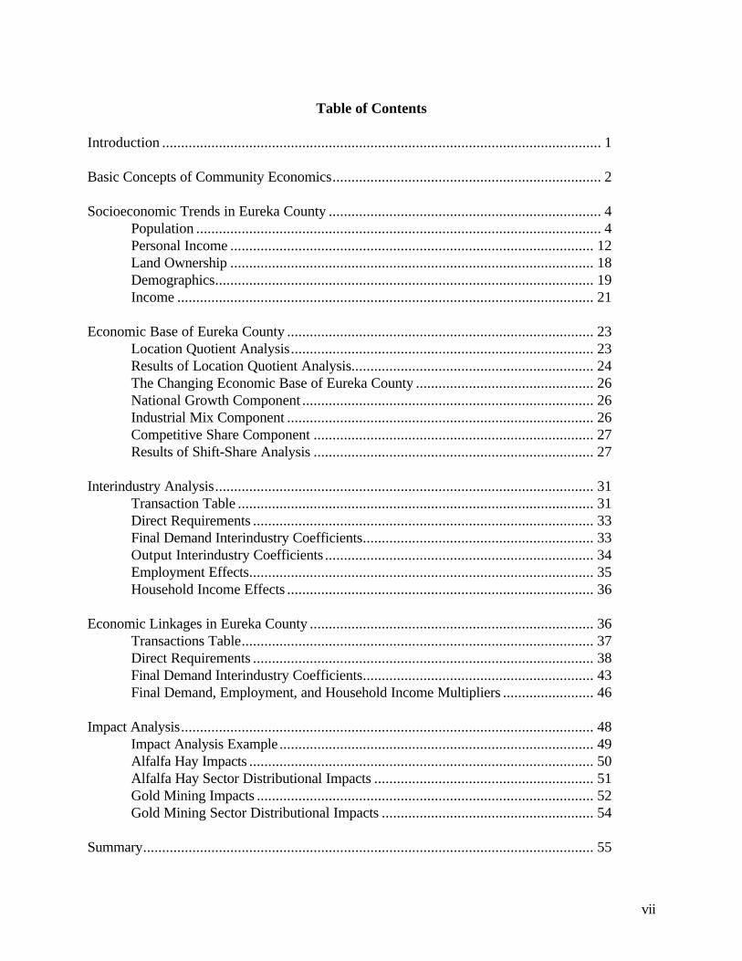
Table of Contents

Introduction .................................................................................................................... 1

Basic Concepts of Community Economics....................................................................... 2

Socioeconomic Trends in Eureka County ........................................................................ 4Population ........................................................................................................... 4Personal Income ................................................................................................ 12Land Ownership ................................................................................................ 18Demographics.................................................................................................... 19Income .............................................................................................................. 21

Economic Base of Eureka County ................................................................................. 23Location Quotient Analysis................................................................................ 23Results of Location Quotient Analysis................................................................ 24The Changing Economic Base of Eureka County ............................................... 26National Growth Component ............................................................................. 26Industrial Mix Component ................................................................................. 26Competitive Share Component .......................................................................... 27Results of Shift-Share Analysis .......................................................................... 27

Interindustry Analysis.................................................................................................... 31Transaction Table .............................................................................................. 31Direct Requirements .......................................................................................... 33Final Demand Interindustry Coefficients............................................................. 33Output Interindustry Coefficients ....................................................................... 34Employment Effects........................................................................................... 35Household Income Effects ................................................................................. 36

Economic Linkages in Eureka County ........................................................................... 36Transactions Table............................................................................................. 37Direct Requirements .......................................................................................... 38Final Demand Interindustry Coefficients............................................................. 43Final Demand, Employment, and Household Income Multipliers ........................ 46

Impact Analysis............................................................................................................. 48Impact Analysis Example ................................................................................... 49Alfalfa Hay Impacts ........................................................................................... 50Alfalfa Hay Sector Distributional Impacts .......................................................... 51Gold Mining Impacts ......................................................................................... 52Gold Mining Sector Distributional Impacts ........................................................ 54

Summary....................................................................................................................... 55

viii

References .................................................................................................................... 56

Appendix A: Listing of Economic Sectors .................................................................... 57

Appendix B: Sources of Data for Eureka CountyInput-Output Model ................................................................................ 59

Appendix C: Private Sector, Local Government and Non-MarketImpacts from Economic Changes............................................................. 61

ix

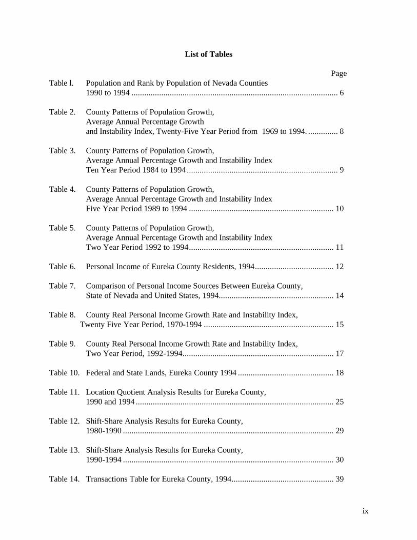
List of Tables

PageTable l. Population and Rank by Population of Nevada Counties

1990 to 1994 ................................................................................................. 6

Table 2. County Patterns of Population Growth,Average Annual Percentage Growthand Instability Index, Twenty-Five Year Period from 1969 to 1994. .............. 8

Table 3. County Patterns of Population Growth,Average Annual Percentage Growth and Instability IndexTen Year Period 1984 to 1994 ....................................................................... 9

Table 4. County Patterns of Population Growth,Average Annual Percentage Growth and Instability IndexFive Year Period 1989 to 1994 .................................................................... 10

Table 5. County Patterns of Population Growth,Average Annual Percentage Growth and Instability IndexTwo Year Period 1992 to 1994.................................................................... 11

Table 6. Personal Income of Eureka County Residents, 1994..................................... 12

Table 7. Comparison of Personal Income Sources Between Eureka County,State of Nevada and United States, 1994...................................................... 14

Table 8. County Real Personal Income Growth Rate and Instability Index,Twenty Five Year Period, 1970-1994 ............................................................. 15

Table 9. County Real Personal Income Growth Rate and Instability Index,Two Year Period, 1992-1994....................................................................... 17

Table 10. Federal and State Lands, Eureka County 1994 ............................................. 18

Table 11. Location Quotient Analysis Results for Eureka County,1990 and 1994 ............................................................................................. 25

Table 12. Shift-Share Analysis Results for Eureka County,1980-1990 ................................................................................................... 29

Table 13. Shift-Share Analysis Results for Eureka County,1990-1994 ................................................................................................... 30

Table 14. Transactions Table for Eureka County, 1994................................................ 39

x

Table 15. Direct Requirements Table for Eureka County, 1990.................................... 41

Table 16. Final Demand Requirements Table from Changes in Final DemandEureka County, 1990 ................................................................................... 44

Table 17. Final demand, Employment, and Income Multipliers forEureka County, 1990 ................................................................................... 47

Table 18. Total Impacts from a Ten Percent Increase in Export Sales by theAlfalfa Hay and Gold Mining Sectors in Eureka County ............................... 50

Table 19. Sectoral Impacts from a Ten Percent Increase in Export Salesby the Alfalfa Hay Sector in Eureka County ................................................. 51

Table 20. Distributional Impacts from a Ten Percent Increase in Export Salesby the Alfalfa Hay Sector in Eureka County ................................................. 52

Table 21. Sectoral Impacts from a Ten Percent Increase in Export Salesby the Gold Mining Sector, Eureka County .................................................. 53

Table 22. Distributional Impacts from a Ten Percent Increase in Export Salesby the Gold Mining Sector in Eureka County ............................................... 54

xi

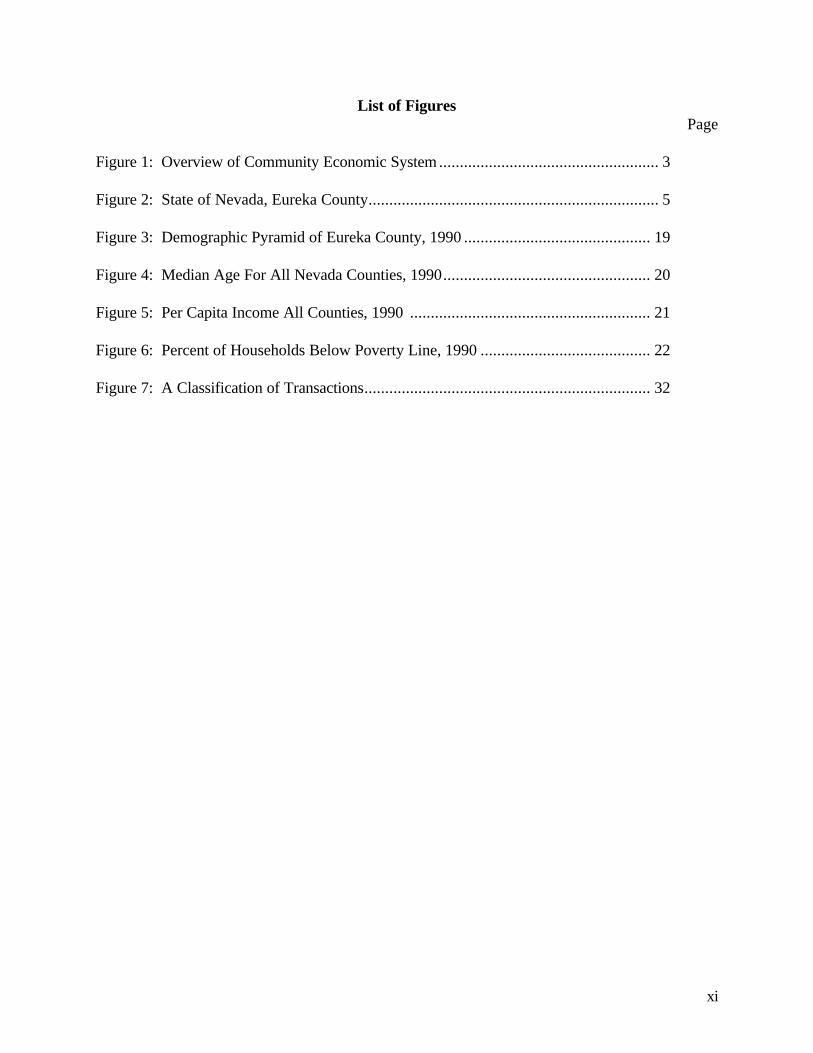
List of FiguresPage

Figure 1: Overview of Community Economic System ..................................................... 3

Figure 2: State of Nevada, Eureka County...................................................................... 5

Figure 3: Demographic Pyramid of Eureka County, 1990 ............................................. 19

Figure 4: Median Age For All Nevada Counties, 1990.................................................. 20

Figure 5: Per Capita Income All Counties, 1990 .......................................................... 21

Figure 6: Percent of Households Below Poverty Line, 1990 ......................................... 22

Figure 7: A Classification of Transactions..................................................................... 32

Introduction

From 1990 to 1994, Eureka County experienced a slight increase in population and real

per capita income. County real per capita income increased by 1.1 percent while county

population increased from 1,550 in 1990 to 1,580 in 1995 or an increase of 1.9 percent. The

Eureka County economy, however, is based on a single industry, mining. In 1990 the mining

sector made up 85.5 percent of total Eureka County employment which has declined to 82.3

percent of total Eureka County employment. Therefore any changes in mining activity will greatly

impact the economy of Eureka County in 1995. Providing information to help local decision

makers understand how external factors could impact the Eureka County economy is the primary

objective of this study.

The general objective of this study is to perform an interindustry analysis and develop an

input-output model for the Eureka County economy. This input-output model calculates the

economic interrelationships, more commonly called linkages, between economic sectors in the

county economy. These linkages are then used to estimate economic impacts on economic

activity, employment, and income in Eureka County from a selected sectoral change in economic

activity. Specific objectives are to:

1) Review the basic concept of community economics;

2) Investigate the socioeconomic trends in Eureka County;

3) Analyze the economic base of Eureka County;

4) Determine the economic linkages within Eureka County; and

5) Perform an impact analysis estimating economic impacts on Eureka County

from increased export sales in the local Alfalfa Hay and Gold Mining Sectors.

The organization of this report follows the sequence of these specific objectives.

2

Basic Concepts of Community Economics

Community economics is an applied field of economics that investigates the

interrelationships, more commonly called linkages, that exist among economic sectors within a

local economy. An overview of a community economic system is presented in Figure 1.

Economic sectors shown are basic industries, households and service firms. The linkages that

exist among these sectors are depicted by Figure 1.

Basic industries are those industries which produce goods and services primarily for sale

outside the economy. These industries are usually involved in agriculture, mining, manufacturing,

or casino gaming. Household and service firms support basic industries. Labor is purchased from

households and inputs are purchased from service firms. Service firms also provide goods and

services to households (consumers). Of course, each of these three sectors purchase products,

inputs and labor from outside the community borders. Local transactions determine the

relationship that exists among the various types of firms in an economy. These three sectors are

also linked with the rest of the economy through inflow and outflow of income, inputs and labor,

goods and services and finished products.

The total impact of any basic industry on an economy consists of direct, indirect and

induced impacts. Direct impacts are the activities or changes in production level of the impacted

industry. Indirect impacts occur in the local business sector as a result of providing inputs to the

impacted industry. For example, the increased output of local firms providing inputs for a local

mining operation represent the indirect impacts of a basic industry. Induced impacts consist of the

economic activity caused by household consumption in a local economy from the direct and

indirect effects.

The relationships discussed above indicate how basic industries serve as the foundation of

an economy and how households and service firms are necessary to make the economy function.

Service industries account for a substantial part of the output of most economies, but, as shown in

Figure 1, much of service industry’s output goes to support local basic industries and households.

Mathematical techniques, such as input-output analysis, can be used to measure the relationships

between basic industries, households and service firms.

3

PRODUCTS

INPUTSLABOR

$

$

$

$

$

$

$

Goods &Services

Inputs &

Labor

Inputs &Labor

HouseholdsService

Basic

Industry

Products

$

Products

$

Labor

Firms

Figure 1: Overview of Community Economic System

4

Socioeconomic Trends in Eureka County

Socioeconomic trends within Eureka County are provided to give a socioeconomic

perspective of Eureka County in comparison to other Nevada counties, as well as state and

national trends. Population, personal income, land ownership, demographics and per capita

income trends are identified in this section.

Population

Eureka County is located in Northeast Nevada approximately 115 miles southwest of Elko

and 240 miles east of Reno. The county is bordered to the west by Lander County, to the north

and east by Elko County, to the east by White Pine County and the south by Nye County. This

location is shown in figure 2. Eureka is the county seat and the primary population center for the

county. Population was estimated to be 1,580 in 1995 which ranks Eureka County seventeenth of

seventeen counties in Nevada. In 1990, Eureka was ranked sixteenth of seventeen Nevada

counties. (Nevada State Demographer, 1997)

5

Figure 2. State of Nevada, Eureka County

6

Table 1. Population and Rank by Population of Nevada Counties from 1990 to 1995.

1995 1990

County Population Rank Population Rank

Clark 1,192,200 1 770,280 1Washoe 311,340 2 257,120 2Carson City 46,770 3 40,950 3Elko 43,050 4 33,770 4Douglas 35,880 5 28,070 5Lyon 26,580 6 20,590 6Nye 23,050 7 18,190 7Churchill 21,640 8 18,100 8Humboldt 16,270 9 13,020 9White Pine 9,770 10 9,410 10Mineral 6,700 11 6,470 11Lander 6,410 12 6,340 12Pershing 5,140 13 4,550 13Lincoln 4,110 14 3,810 14Storey 3,200 15 2,560 15Esmeralda 1,630 16 1,350 17Eureka 1,580 17 1,550 16

Source: Nevada State Demographer’s Office. “Population of Nevada’s Counties and IncorporatedCities.” College of Business Administration, University of Nevada, Reno, February 1997.

7

To investigate trends, population growth was estimated from 1969 to 1995 (a twenty-six

year period), 1985 to 1995 ( a ten year period), 1990 to 1995 (a five year period) and 1993 to

1995 (a two year period). The period 1969 to 1995 was chosen because it aligns with the

historical data series provided by the Regional Economic Information System population,

employment, and income data (U.S. Department of Commerce, 1997). Also different periods of

analysis were analyzed to discern if any changes in trends have occurred.

From Table 2, Eureka County ranked fourteenth among Nevada’s seventeen counties in

average annual percentage growth rate. However, Eureka County ranked third highest in

instability of population growth during the twenty-six year study period.

For the ten year period from 1985 to 1995, Eureka County ranked fourteenth among

Nevada’s seventeen counties in average annual growth rate (Table 3). However, during this ten

year period, Eureka County ranked third highest in instability of growth rates.

For the five year time period from 1990 to 1995, average annual growth rate for Eureka

County ranked sixteenth among Nevada’s seventeen counties (Table 4). However, during this

five year study period, Eureka County had the highest rank in instability of annual growth rates.

From 1993 to 1995, Eureka County was one of three Nevada counties to experience

negative average annual population growth rate. The county’s average annual growth rate was

the lowest of all seventeen counties in Nevada (Table 5). The instability index for annual growth

rates ranked Eureka County as third highest of Nevada’s seventeen counties during this two year

study period.

8

Table 2. County Patterns of Population Growth, Average Annual Percentage Growth and Instability Index, Twenty-Six Year Period (1969-1995).

County Average Annual% Change

CountyRank

InstabilityIndex

CountyRank

Douglas 6.72 1 0.62 14Storey 6.18 2 0.89 10Nye 5.78 3 1.29 8Clark 5.35 4 0.28 17Lyon 4.79 5 0.49 15Esmeralda 4.79 6 2.53 4Carson City 4.49 7 0.78 11Elko 4.47 8 0.90 9Humboldt 3.72 9 0.76 13Lander 3.71 10 1.79 7Washoe 3.54 11 0.35 16Churchill 2.89 12 0.77 12Pershing 2.63 13 1.29 5Eureka 2.35 14 2.87 3Lincoln 2.08 15 2.01 6White Pine -0.04 16 103.06 1Mineral -0.19 17 13.34 2

Nevada 4.70 0.25

UnitedStates 1.03 0.13

Source: Nevada State Demographer’s Office. “Population of Nevada’s Counties and Incorporated Cities.”College of Business Administration, University of Nevada, Reno, Various Issues.

9

Table 3. County Patterns of Population Growth, Average Annual Percentage Growth and Instability Index, Ten Year Period (1985 - 1995)


CountyRank

InstabilityIndex

CountyRank

Elko 6.85 1 0.61 12Clark 6.32 2 0.24 17Storey 5.72 3 0.77 8Lyon 4.92 4 0.27 16Nye 4.75 5 0.74 9Douglas 4.59 6 0.69 10Humboldt 3.77 7 0.51 13Lander 3.75 8 1.77 4Churchill 3.68 9 0.66 11Pershing 3.49 10 0.82 7Carson 2.76 11 0.44 14Washoe 2.74 12 0.41 15White Pine 2.44 13 1.28 6Eureka 2.05 14 2.04 3Lincoln 0.88 15 3.21 2Mineral 0.82 16 1.67 5Esmeralda 0.78 17 8.55 1

Nevada 5.18 0.21

UnitedStates 1.00 0.08


10

Table 4. County Patterns of Population Growth, Average Annual Percentage Growth and Instability Index, Five Year Period (1990 - 1995).


CountyRank

InstabilityIndex

CountyRank

Clark 6.12 1 0.23 15Lyon 5.24 2 0.20 16Douglas 5.12 3 0.86 8Elko 4.98 4 0.17 17Nye 4.91 5 0.71 10Storey 4.60 6 0.81 9Humboldt 4.57 7 0.35 14Esmeralda 4.12 8 1.86 5Churchill 3.65 9 0.38 13Washoe 2.74 10 0.41 12Carson 2.70 11 0.52 11Pershing 2.51 12 1.22 7Lincoln 1.60 13 2.41 4White Pine 0.79 14 3.30 2Mineral 0.72 15 2.86 3Eureka 0.45 16 7.83 1Lander 0.22 17 1.72 6

Nevada 5.07 0.23

UnitedStates

1.06 0.06


11

Table 5. County Patterns of Population Growth, Average Annual Percentage Growth and Instability Index, Two Year Period (1993 – 1995)


CountyRank

InstabilityIndex

CountyRank

Esmeralda 11.28 1 0.53 9Douglas 8.79 2 0.59 6Clark 7.43 3 0.10 15Nye 6.03 4 0.85 5Storey 6.01 5 0.52 10Humboldt 5.91 6 0.32 11Lyon 5.80 7 0.19 13Pershing 4.72 8 0.55 7Elko 4.61 9 0.06 16Churchill 4.41 10 0.18 14Washoe 4.06 11 0.02 17Carson 3.74 12 0.29 12Mineral 1.49 13 1.93 4White Pine 1.28 14 3.13 2Lincoln -0.11 15 48.35 1Lander -0.16 16 0.53 8Eureka -2.06 17 1.94 3

Nevada 6.36 0.07

UnitedStates

1.06 0.06


12

Personal Income

In 1995, Eureka County residents received approximately $33.3 million in personal

income. Approximately $260.6 million was total earnings in the county in the form of wages and

salaries, other labor income, and proprietor’s income. This number is adjusted to net earnings of

approximately $23.7 million by taking into account social security contributions and commuting

adjustments. Approximately $5.0 million was in the form of unearned income from dividends,

interest and rent; and approximately $4.6 million from transfer payments such as social security,

food stamps, unemployment payments, and veteran benefits. These income figures are shown in

Table 6.

Table 6. Personal Income of Eureka County Residents, 1995

- - - - - ($1,000) - - - - -Income Category

Wages and Salaries 216,785Other Labor Income 42,409Proprietor’s Income 1,426

Total Earnings in Eureka County 260,620

Less Personal Social Security Contributions -15,168Plus Residence/Commuting Adjustment -221,712

Net Earnings of Eureka CountyResidents

23,740

Dividends, Interest and Rent 5,002Transfer Payment 4,592

Total Personal Income, Eureka CountyResidents

33,334

Eureka County 1995Per Capita Income (Dollars)

23,165

Source: U.S. Department of Commerce. “Regional Economic Information System.” Bureau of EconomicAnalysis, Washington, D.C., August 1997.

To more accurately measure income available to Eureka County residents before income

taxes (a concept called personal income by economists), approximately $15.2 million of personal

contributions to social insurance programs such as Social Security, Medicare, Unemployment, etc.

paid by residents of Eureka County must be subtracted. Subtracting personal insurance

13

contributions and resident adjustments leaves net earnings of Eureka County residents of over

$23.7 million, or approximately 71 percent of total personal income.

A commuting adjustment is made to total earnings since some people who earn income in

Eureka County are not county residents. These people commute into the county to work and

take their paycheck back home. Some Eureka County residents also work outside the county and

bring income back to the county. The difference between what is earned outside Eureka County

and injected back into the county and what is earned in Eureka County and leaves the county is

over -$221.7 million. The large negative net residence adjustment factor for Eureka County is

due to the Mining Sector workers who work in northern Eureka County but live in Elko.

Table 7 gives the percentage breakdown of Eureka County’s income by source and

presents similar data for the state of Nevada and the nation. Eureka County’s breakdown differs

from the state of Nevada and nation. Net earnings by residents for Eureka County are

approximately 71% of total personal income as opposed to approximately 69% and 66% for the

state of Nevada and the United States, respectively. Dividends, interest and rents account for a

smaller percentage of total Eureka County income as well as the proportional share of total

personal income from transfer payments is lower for Eureka County.

Eureka County’s per capita income is lower than that of the state or nation. At $23,165

Eureka County’s 1995 income per capita was approximately 5% less than the state’s $24,361 and

approximately 1% less than the national average of $23,196.

14

Table 7. Comparison of Personal Income Sources between Eureka County, State of Nevada, and United States, 1995.

Personal Income SourceEureka County

(%)Nevada

(%)United States

(%)

Wages and Salaries 650.3 60.5 56.1

Other Labor Income 127.2 6.3 6.9

Proprietor’s Income 4.3 8.0 7.7

Less Personal Social InsuranceContributions

-45.5 -4.5 -4.8

Plus Residence/Commuting Adjustments -665.1 -1.4 0.0

Net Earnings of Residents 71.2 68.9 65.9

Dividends, Interest and Rents 15.0 16.7 17.3

Transfer Payments 13.8 14.4 16.8

Total Personal Income 100.0 100.0 100.0

Per Capita Personal Income $23,165 $24,361 $23,196


15

The twenty-six year pattern of real personal income growth is provided in Table 8. Total

personal income for Eureka County had an average annual growth rate of 2.45 percent for the

period of 1969 to 1995. This ranks the county fifteenth among Nevada’s seventeen counties.

This annual growth rate was lower than the growth rate of the state of Nevada and the national

average. Eureka County also ranks the highest of all seventeen Nevada counties according to the

instability index. This high instability statistic signifies that Eureka County has had a somewhat

unstable economy when compared to other Nevada counties. Being so dependent upon one

economic sector contributes to this instability.

Table 8. County Real Personal Income Growth Rate and Instability Index, Twenty SixYear Period (1969 to 1995). a


CountyRank

InstabilityIndex

CountyRank

Douglas 7.76 1 0.60 16Storey 6.84 2 0.94 12Clark 6.70 3 0.44 17Carson 6.37 4 0.69 15Nye 6.02 5 1.07 10Lyon 5.78 6 0.74 13Elko 5.77 7 1.04 11Humboldt 5.49 8 1.39 8Lander 5.40 9 1.71 7Washoe 5.33 10 0.71 14Churchill 4.90 11 1.11 9Esmeralda 4.76 12 3.55 4Lincoln 3.73 13 1.87 6Pershing 2.78 14 3.78 3Eureka 2.45 15 4.47 1White Pine 1.72 16 4.21 2Mineral 1.26 17 3.47 5

Nevada 6.15 0.49

United States2.96 0.61

a Real incomes determined using the Implicit Price Deflator for Personal Consumption Expenditures, 1992 = 100.

Source: U.S. Department of Commerce. “Regional Economic Information System.” Bureau of EconomicAnalysis, Washington, D.C. August 1997.

16

The two year pattern of real personal income growth is provided in Table 9. Total real

personal income for Eureka County had a negative average annual growth rate of –2.16. Eureka

County was one of three Nevada counties that realized negative total personal income growth

over the period between 1993 and 1995. The state of Nevada had the highest growth rate of all

states in the nation, but as Table 9 shows, this growth was disproportionately shared among

Nevada counties. Eureka County ranked sixteenth among Nevada’s seventeen counties in

average annual growth rate of real total income from 1993 to 1995. Eureka County also ranked

seventh highest in terms of instability of real total personal income growth signifying that during

this period Eureka County had fairly unstable growth when compared to other counties in

Nevada, the state of Nevada and the nation.

17

Table 9. County Real Personal Income Growth and Instability Index, Two Year Period (1993 to 1995). a

County Average AnnualGrowth Rate (%)

CountyRank

InstabilityIndex

CountyRank

Nye 11.55 1 0.04 15White Pine 9.05 2 0.29 8Clark 8.31 3 0.09 12Storey 6.55 4 0.10 11Douglas 5.95 5 0.17 10Carson City 5.94 6 0.05 14Washoe 5.64 7 0.04 16Lyon 5.28 8 0.18 9Churchill 4.45 9 0.09 13Elko 4.25 10 0.49 6Humboldt 3.71 11 0.55 5Pershing 2.23 12 1.65 3Lander 1.73 13 1.32 4Mineral 0.94 14 3.63 1Lincoln -1.77 15 0.01 17Eureka -2.16 16 0.31 7Esmeralda -2.30 17 2.01 2

Nevada 7.27 0.06

UnitedStates

3.12 0.17

a Real incomes determined using the Implicit Price Deflator for Personal Consumption Expenditures, 1992 = 100.

Source: U.S. Department of Commerce. “Regional Economic Information System.” Bureau of EconomicAnalysis, Washington, D.C. August 1997.

18

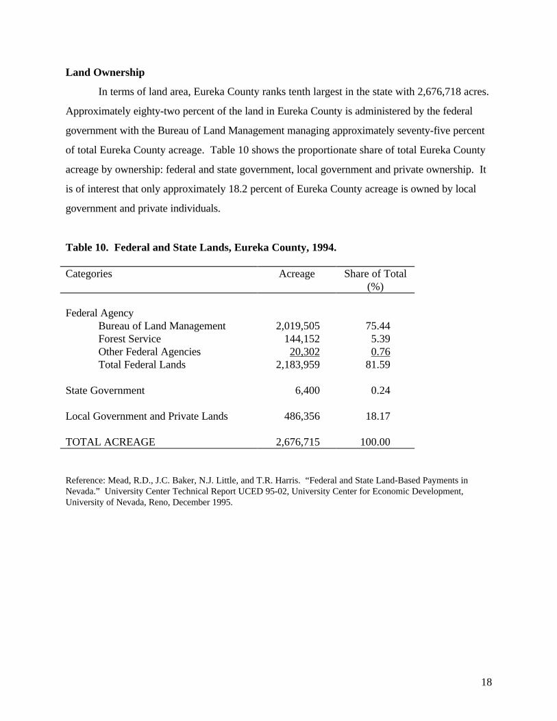
Land Ownership

In terms of land area, Eureka County ranks tenth largest in the state with 2,676,718 acres.

Approximately eighty-two percent of the land in Eureka County is administered by the federal

government with the Bureau of Land Management managing approximately seventy-five percent

of total Eureka County acreage. Table 10 shows the proportionate share of total Eureka County

acreage by ownership: federal and state government, local government and private ownership. It

is of interest that only approximately 18.2 percent of Eureka County acreage is owned by local

government and private individuals.

Table 10. Federal and State Lands, Eureka County, 1994.

Categories Acreage Share of Total(%)

Federal AgencyBureau of Land Management 2,019,505 75.44Forest Service 144,152 5.39Other Federal Agencies 20,302 0.76Total Federal Lands 2,183,959 81.59

State Government 6,400 0.24

Local Government and Private Lands 486,356 18.17

TOTAL ACREAGE 2,676,715 100.00

Reference: Mead, R.D., J.C. Baker, N.J. Little, and T.R. Harris. “Federal and State Land-Based Payments inNevada.” University Center Technical Report UCED 95-02, University Center for Economic Development,University of Nevada, Reno, December 1995.

19

Demographics

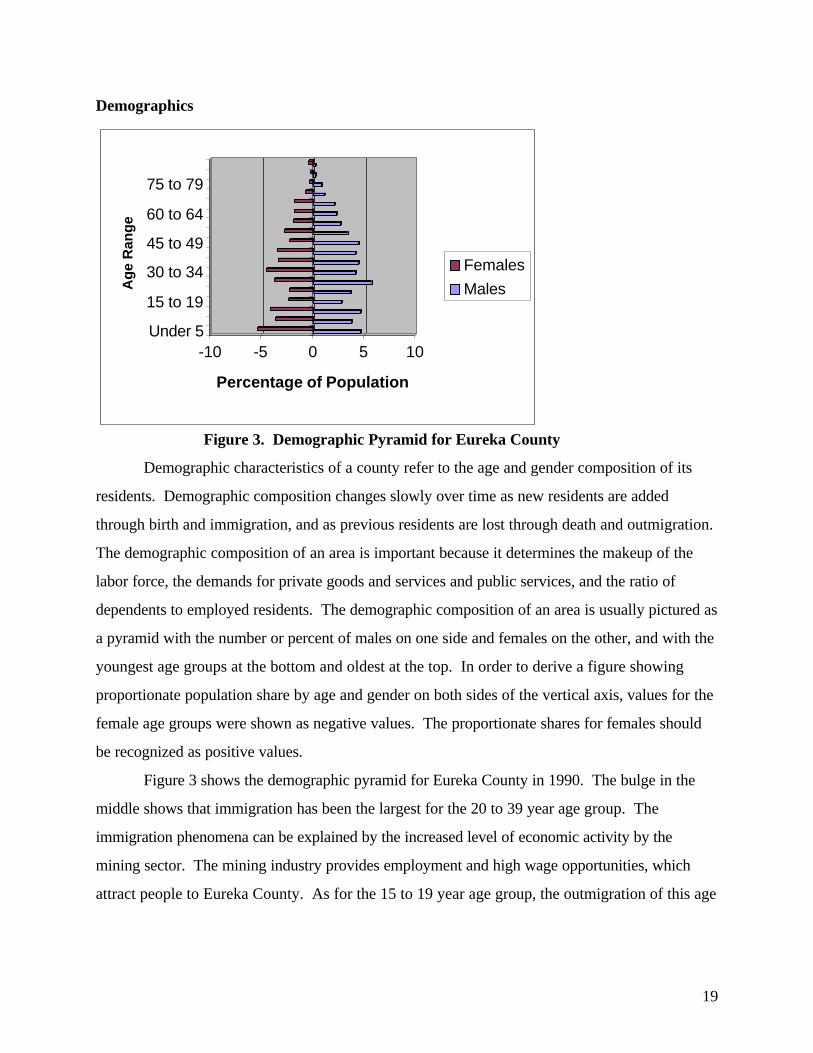
Figure 3. Demographic Pyramid for Eureka County

Demographic characteristics of a county refer to the age and gender composition of its

residents. Demographic composition changes slowly over time as new residents are added

through birth and immigration, and as previous residents are lost through death and outmigration.

The demographic composition of an area is important because it determines the makeup of the

labor force, the demands for private goods and services and public services, and the ratio of

dependents to employed residents. The demographic composition of an area is usually pictured as

a pyramid with the number or percent of males on one side and females on the other, and with the

youngest age groups at the bottom and oldest at the top. In order to derive a figure showing

proportionate population share by age and gender on both sides of the vertical axis, values for the

female age groups were shown as negative values. The proportionate shares for females should

be recognized as positive values.

Figure 3 shows the demographic pyramid for Eureka County in 1990. The bulge in the

middle shows that immigration has been the largest for the 20 to 39 year age group. The

immigration phenomena can be explained by the increased level of economic activity by the

mining sector. The mining industry provides employment and high wage opportunities, which

attract people to Eureka County. As for the 15 to 19 year age group, the outmigration of this age

-10 -5 0 5 10

Percentage of Population

Under 5

15 to 19

30 to 34

45 to 49

60 to 64

75 to 79

Ag

e R

ang

e

Females

Males

20

group can be attributed to young adults leaving the county for entry level employment

opportunities or higher education.

Another aspect of demographics for Eureka County is the median age of population. In

Figure 4, the median age for Eureka County is 35.8 years, which is a little older than the state’s

median age of 33.3 years.

0

5

10

15

20

25

30

35

40

Car

son

City

Dou

glas

Esm

eral

da

Eur

eka

Hum

bold

t

Land

er

Linc

oln

Lyon

Min

eral

Nye

Per

shin

g

Sto

rey

Was

hoe

Whi

te P

ine

Figure 4. Median Age for All Nevada Counties, 1990

The demographic characteristics of Eureka County are somewhat similar to many rural

counties in the nation. Often rural counties have higher median age values because the young

people with the best education and health, and the most marketable skills and abilities, leave the

rural area to realize their potential. With them go some of the area’s future leaders, innovators,

and entrepreneurs. Taxes collected in the county, to invest in their education, are now earning

dividends for people and economies in other counties and states.

21

Income

Economic quality of life is difficult to measure because of differences in cost of living and

non-monetary income between locations. However, per capita income is still an important basis

for comparing economic quality of life, especially among geographically similar areas. On this

basis, the economic quality of life in Eureka County was relatively high in 1990. In Figure 5, the

per capita income of each county is shown and in comparison to Eureka County, the counties of

Douglas, Esmeralda, and Washoe had higher per capita incomes.

$0

$5,000

$10,000

$15,000

$20,000

$25,000

$30,000

$35,000

Car

son

City

Chu

rchi

ll

Cla

rk

Dou

glas

Elk

o

Esm

eral

da

Eur

eka

Hum

bold

t

Land

er

Linc

oln

Lyon

Min

eral

Nye

Per

shin

g

Sto

rey

Was

hoe

Whi

te P

ine

Nev

ada

Figure 5. Per Capita Income All Counties, 1990

Another useful measure of economic quality of life is the percent of households below the

poverty line. From Figure 6, Eureka County in 1990 had shown a level of poverty that was lower

than many of Nevada’s other counties. The percentage of families living below the poverty line in

Eureka County in 1990 was 7.4 percent. This ranked Eureka County as the fourth lowest county

in percent of families below the poverty line. As comparison, the percentage of families living

22

below the poverty line was 7.3 percent for the state, while the nation’s percentage of families

living below the poverty line was 10.0% in 1990.

0.00%

2.00%

4.00%

6.00%

8.00%

10.00%

12.00%

14.00%

16.00%

18.00%

20.00%

Chu

rchi

ll

Cla

rk

Dou

glas

Elk

o

Esm

eral

da

Eur

eka

Hum

bold

t

Land

er

Linc

oln

Lyon

Min

eral

Nye

Per

shin

g

Sto

rey

Was

hoe

Whi

te P

ine

Figure 6. Percent of Households Below Poverty Line, 1990

23

The Economic Base of Eureka County

The economic base of a county refers to the relative size of its industries. A county is said

to have a diversified economic base if several industries are relatively large. Conversely, if one or

a few industries dominate a local economy, the economy is said to have a concentrated economic

base. There are two techniques used to measure economic base and changes in economic base.

These are location quotient analysis and shift-share analysis.

Location Quotient Analysis

The degree of concentration of Eureka County industries is determined by calculating

location quotients for individual economic sectors. Location quotients indicate the economic

importance of each regional industry relative to the same industry at the national level. Location

quotients usually use employment as an indicator of an industry’s size and importance. The

primary focus of location quotients is to identify the industries which are either more important or

less important locally than nationally. The broader the economic base, that is, the higher the

location quotients, the more stable the economy of a community. On the other hand, very low

location quotients represent industries that are largely underdeveloped and may offer an

opportunity for future development.

An industry’s location quotient is the ratio of the industry’s share of employment in the

county to the industry’s share of employment in the nation. It is calculated as follows:

LQe E

n Nii

i

=/

/

where:

i = Economic Sector

LQ i = Location quotient for economic sector i

e i = County employment in economic sector i

E = Total county employment

n i = National employment in economic sector i

N = Total national employment

24

The interpretation of location quotients are as follows:

1. Every industry’s output can be divided into two uses: export and local consumption

(use).

2. The amount consumed (used) by an community is proportionate to the amount

consumed locally.

3. If the location quotient for an economic sector is less than one, goods and services

must be imported to satisfy local demands.

4. If the location quotient for an economic sector is equal to one, then the economy is

approximately fulfilling the requirements of the local household and firms.

5. Finally, if the location quotient is greater than one, for that particular economic sector,

the community is producing more than it consumes and is capable of exporting excess

goods for the purposes of bringing income into the community.

Results of Location Quotient Analysis

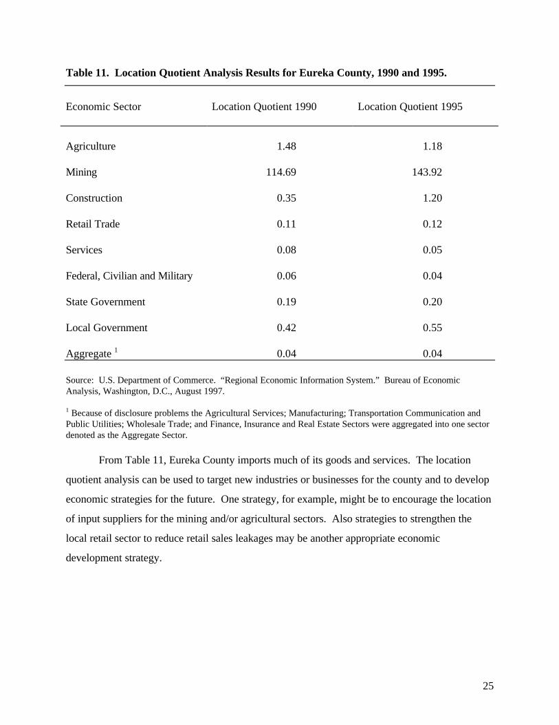
Location quotients shown in Table 11 were derived from employment levels in each

economic sector at county and national levels from the U.S. Department of Commerce, Regional

Economic Information System, for 1990 and 1995.

Given the interpretation of location quotients, economic sectors in Eureka County can be

classified as export sectors (that is, they market much of their output outside the county in which

they are located) or import industries (that is, a large portion of the demand for goods and

services is satisfied by producers outside the county).

The location quotient analysis for Eureka County’s economic base for 1990 and 1995

indicates that the county is highly dependent on Mining, and Agricultural Sectors. The Mining

Sector had the highest location quotient value of 143.92 in 1995 showing the importance of the

Mining Sector to the local economy. Also, because of disclosure problems the Agriculture

Services; Manufacturing; Transportation Communication and Public Utilities; Wholesale Trade;

and Finance, Insurance and Real Estate Sectors were aggregated into a single sector.

25

Table 11. Location Quotient Analysis Results for Eureka County, 1990 and 1995.

Economic Sector Location Quotient 1990 Location Quotient 1995

Agriculture 1.48 1.18

Mining 114.69 143.92

Construction 0.35 1.20

Retail Trade 0.11 0.12

Services 0.08 0.05

Federal, Civilian and Military 0.06 0.04

State Government 0.19 0.20

Local Government 0.42 0.55

Aggregate 1 0.04 0.04


1 Because of disclosure problems the Agricultural Services; Manufacturing; Transportation Communication andPublic Utilities; Wholesale Trade; and Finance, Insurance and Real Estate Sectors were aggregated into one sectordenoted as the Aggregate Sector.

From Table 11, Eureka County imports much of its goods and services. The location

quotient analysis can be used to target new industries or businesses for the county and to develop

economic strategies for the future. One strategy, for example, might be to encourage the location

of input suppliers for the mining and/or agricultural sectors. Also strategies to strengthen the

local retail sector to reduce retail sales leakages may be another appropriate economic

development strategy.

26

The Changing Economic Base of Eureka County

The location quotient results indicate the nature of the area’s economy for a specific time

period. Of additional interest is the change occurring in the county’s economic base. Shift-share

analysis is performed to measure these changes.

Shift-share analysis, like location quotients, is a measure of a county’s economic condition

relative to other communities and to the nation as a whole. The data used in this analysis are the

same as that used for the location quotient analysis. For this study, the shift in economic base was

studied from 1980 to 1990 and 1990 to 1995.

The purpose of shift-share analysis is to determine the county’s competitiveness and

changing employment patterns in the industrial market place. Shift-share analysis assumes that

there are three components to changes in employment: national growth, industrial mix and

competitive share.

National Growth Component

The sum of employment in all industries in all communities makes up national

employment. One would expect that if a community’s economy was maintaining its relative

competitiveness, changes in the level of national employment would be reflected in

proportionately equal changes in the local employment. The calculation of the national growth

component, therefore, measures how much of the local employment change is due to the national

growth trend. The calculation is as follows:

National Growth Component = (rate of change in N e i* )

where:

rate of change in nation or N = ( )N N

N1990 1980

1980

−

e i = county employment in economic sector i

Industrial Mix Component

On a national level, each industry grows or declines at some rate, at least partially

independent of the rate of growth in the national economy. A local economy’s performance will

depend, on its mix of industries, that is, on whether its economic base is concentrated in faster or

27

slower growing industries. The industrial mix calculation indicate the expected growth in local

industries if they grow at the same rate as their national counterparts. The expected local share of

the particular industry is determined using the following equation:

Industrial Mix Component = (rate of change in n i − rate if change N) * e i

n i = national employment in economic sector i

N = total national employment


rate of change in nn n

nii i

i

=−( )1990 1980

1980

Competitive Share Component

A local industry’s employment grows or declines for a number of reasons, including

changes in the national employment level, changes in employment by the same industry at the

national level, and changes in local conditions. After the first two components have been

calculated, the residual change, if any, is attributed to changes in the competitiveness of the local

industry. The competitive share component measures this latter factor in employment change.

The competitive share component is measured as follows:

Competitive Share = (rate of change in e i - rate of change in n i ) * e i

where:


rate of change in ee e

eii i

i

=−1990 1980

1980

rate of change in nn n

nii i

i

=−1990 1980

1980

Results of Shift-Share Analysis

A local industry’s employment grows or declines for a number of reasons, including

changes in the national employment level, changes in employment by the same industry at the

national level, and changes in local conditions. After the national component and industrial mix

component have been calculated, the residual change, if any, is attributed to changes in the

28

competitiveness of the local industry. Tables 12 and 13 show the results of the shift-share analysis

for Eureka County for the periods 1980 to 1990 and 1990 to 1995.

From Table 12, Eureka County overall employment increased by 3,242 from 1980 to

1990. The Mining Sector was by far the leading economic sector in growth with the Mining

Sector accounting for approximately ninety-nine percent of total county growth from 1980 to

1990. Nationally, mining lost employment from 1980 to 1990. However, the competitive

advantage of the Mining Sector in Eureka County provided for most of the overall employment

growth in Eureka County.

For the Retail Sector, national and industrial mix growth rates contributed to positive

growth in this local sector. However, the negative competitive share contributed to overall

decline in retail trade. An economic development strategy would be to investigate the causes for

this negative competitive share and if possible correct the non-competitiveness of this sector.

From Table 13, overall employment in Eureka County increased by 624 jobs from 1990 to

1994. The Mining and Construction Sectors contributed most to growth in Eureka County. This

is due to expanded mining operations and construction related to mining operations and housing.

As opposed to Table 12, the Retail Trade Sector realized employment growth during 1990 to

1995 and had a positive competitive share during this five year period. However, the Service

Sector realized employment loss from 1990 to1995 and had the largest negative Competitive

Share of all economic sectors in Eureka County.

Overall, Eureka County realized employment growth between 1980 and 1990 and from

1990 to 1995. National growth component impacted Eureka County employment positively for

these two study periods. For both time periods, the Mining Sector was a major contributor to

county employment growth. Analyzing results of both the location quotients and shift-share

analysis, Eureka County is highly dependent on the Mining Sector. By diversifying the economic

base of Eureka County, it may be possible to lower cyclical swings in the local economy.

However, in pursuing the goal of economic diversification, the goal of economic growth must

also be addressed.

29

Table 12. Shift-Share Analysis Results for Eureka County, 1980-1995.

Economic Sector NationalComponent

Industrial Mix CompetitiveShare

Total

Agriculture 44 -78 -25 -59

Mining 80 -146 3,278 3,212

Retail 23 6 -62 -33

Services 16 23 -21 18

Federal Government,Military and Civilian

2 -1 -1 0

State Government 0 0 23 23

Local Government 22 -8 21 35

Aggregate 1 20 -10 36 46

TOTAL 207 -214 3,249 3,242



30

Table 13. Shift-Share Analysis Results for Eureka County, 1990 - 1995.

Economic Sector NationalComponent

Industrial Mix CompetitiveShare

Total

Agriculture 34 -40 40 -34

Mining 874 -1,246 763 391

Construction 19 -19 197 197

Retail Trade 18 -16 17 19

Services 22 64 -102 -16

Federal Government,Civilian and Military

2 -3 -2 -3

State Government 6 -5 2 3

Local Government 33 -27 52 58

Aggregate 1 15 -32 26 9

TOTAL 1023 -1,324 925 624



31

Interindustry Analysis

Within a regional economy, there are numerous economic sectors performing different

tasks. All sectors are dependent on each other to some degree. A change in activities will

directly or indirectly affect the response or level of production of the other regional sectors. The

amount of economic activity among economic sectors shows the degree of interrelationships or

linkages between sectors. That is, an increase in production by the regional Livestock Sector

would directly increase purchases of alfalfa hay. With increased alfalfa hay purchases, farm

workers will have greater incomes which would increase their purchases from the Trade Sector.

The Trade Sector would experience increased economic activity because of its indirect

relationship with the Livestock and Alfalfa Hay Sectors. These interdependencies among regional

economic sectors can be estimated through interindustry analysis.

Transaction Table

An interindustry analysis is based on the transactions of the sectors in an economy, i.e.,

purchases of inputs and sales of outputs. A transaction table present in Figure 7 shows the

monetary flows of goods and services through a regional economy. Transactions can be

delineated into four major classifications. One classification (Quadrant I) is the processing section

which produces goods and services. Processing sectors in Quadrant I produce and buy products

and/or services from other processing sectors to be used in their production process. Goods and

services used in the processing section are intermediate goods which are used in the production of

goods and services which are ultimately sold to final consumers.

Another classification (Quadrant II) includes sales to final demand of goods and services.

The Final Demand Section includes net inventory change, exports, government purchases, capital

formation and purchases by households. The third classification (Quadrant III) is the Final

Payment Section. The Final Payments Section includes the non-processing supply sectors such as

imports, depreciation, and households. Quadrant IV represents direct inputs of final demand

which are not produced by industries in the processing sector.

32

Output

Input

Sector

1. . . . . . . . . . j . . . . . . .n Final Demand

l....i....n

.

.

.

.ijX .

. . . . . . . . . . ......

. . . . . . . . .

Quadrant I(Processing Section)

. . . . . . . . . .

Quadrant II(Final Demand Section)

iX

TotalGrossOutput

Final Payments......

Quadrant III(Final Payments Section)

Quadrant IV(Final Demand-Final PaymentsSection)

jX

Total Gross Input

Figure 7. A Classification of Transactions

Transactions include costs and revenues concerning an economic sector. First, reading

down the column of the transactions table, the inputs (cost) required by a specific sector from

other specific sectors to produce its output can be seen. Second, reading across the row of the

transactions table, the distribution of sales by a specific sector to other sectors can be seen.

In Figure 7, a total of n industries are listed across the top and on the left hand side of

Quadrant I. For a given industry i, reading across the row gives the sales of that sector to all

other sectors in the regional economy. For example, the values in the cell where row i intersects

with column j ( )x ij represents the sales of sector i to sector j. The sales of sector i to j are also

purchases of sector j from sector i.

33

Direct Requirements

The logic of interindustry analysis is to establish the structural relationships among the

processing sectors of the model. These relationships can be seen throughout the direct

requirements table. A direct requirement coefficient is computed from the processing section

(Quadrant I) of the transaction table by dividing the value in a column cell by total output of the

column. This can be expressed as:

ax

Xij

ij

j

= i, j = 1, 2, ... , n

where a ij is the purchase by sector j from sector i to produce one dollar of output by sector j,

x ij is the dollar value of transactions between sector i and sector j, and X j is the value of total

output for sector j.

The a ij is a direct requirement coefficient which shows how much a given sector

purchases from another sector within the same regional economy in order to produce one dollar’s

worth of output. Direct requirement coefficients are only calculated for the processing sectors.

The column sum of the direct requirements coefficients of a given sector show the direct

effects of changes in the volume of output of a given sector upon other sectors of the economy.

The direct effect or “first round” effects show how much a given sector has to increase its

purchases of output from other processing sectors when there is an increase in demand for the

output of the given sector.

Final Demand Interindustry Coefficients

Due to the direct effect of additional output for a given industry, other processing sectors

must supply additional inputs. To supply these additional outputs, the directly affected sectors

must increase their output levels which means increased purchases from their input supply sectors.

This expansion of output by sectors directly and indirectly related to the principal sector that

increased its output to meet final demand sales is referred to as a final demand interindustry

coefficient. The column sum of final demand interindustry coefficients derives the final demand

multiplier for a given economic sector. The final demand multiplier estimates the increase in

regional economic activity required for a particular economic sector to increase sales to final

demand by one dollar.

34

Final demand multipliers are calculated for both “open” and “closed” input-output models.

An “open” model does not contain a non-processing sector in the processing section of the

transaction table. The final demand multiplier of an “open” model derives both direct and indirect

effects of a one dollar increase in sales to final demand for a given sector. Indirect effects being

those increases in levels of output for the regional economy to meet the output levels of the

directly related industries.

A “closed” input-output model contains at least one non-processing sector in the

processing section of the transactions model. Usually the Household Sector is incorporated into

the processing section of the transactions table to produce a closed model. The final demand

multiplier from a “closed” model derives direct, indirect, and induced effects from a one dollar

increase in sales to final demand for a given sector. Induced effects are the effects of new

incomes to households upon the individual sectors of the economy from increased sales to final

demand by a given sector.

Output Interindustry Coefficients

Final demand interindustry coefficients derive the effects to the regional economy from

sales to final demand for a given sector. In order to meet these final demand sales, the given

sector must increase production by purchases from itself. This intrasectoral purchasing increases

output response greater than one. In order to estimate economic effects from total production

rather than from deliveries outside the processing sectors, output interindustry coefficients are

required.

Output interindustry coefficients are calculated by dividing each column entry in the final

demand interindustry coefficient matrix by the given sector’s intrasectoral interindustry

coefficient. This will derive intrasectoral coefficients equal to one. The other entries in the final

demand interindustry coefficients matrix are adjusted similarly to refer to production rather than

external end product deliveries by dividing all entries in each row by the entry at the intersection

with the corresponding column or the intrasectoral coefficient.

Direct and indirect output multiplier coefficients are derived from an “open” model.

Indirect effects being the increased purchases in the regional economy created by the purchases of

the directly affected sectors from a given sector’s increase in production. Direct, indirect, and

35

induced output interindustry coefficients are derived from a “closed” model. Induced effects

being the increase in regional economic activity from increase in household incomes created by

production increases for a given sector.

Employment Effects

Interindustry analysis is used to determine the effects on the regional economy from

changes in a given sector’s level of output or sales to final demand. Interindustry analysis also can

be used to derive the effects on regional employment from changes in a given sector’s sales to

final demand or output level. Studies by Elrod and Laferney (1972) and Osborn et al. (1973)

have derived procedures to determine regional employment impacts from input-output models.

To determine employment effects, it is first required that the direct labor effects for each

of the n processing sectors be derived, or:

LE

Xj

j

j

= j = 1, 2, ... , n

where L j is the number of employees required per dollar of output by sector j; E j is the number

of workers employed by sector j; and X j is the dollar value of production by sector j.

From the direct employment requirements vector for each processing sector in the region,

direct and indirect labor requirements from a one dollar sales to final demand by a given sector

can be derived by premultiplying the direct labor coefficients matrix by the “open” final demand

interindustry coefficient matrix. Indirect labor effects are the number of workers employed

elsewhere in the regional economy to produce the direct and indirect inputs used by each sector.

Premultiplying the direct labor requirements matrix by the “closed” interindustry

coefficients matrix derives the direct, indirect, and induced employment effects in the region from

a given sector’s change in sales to final demand interindustry coefficients matrix. Direct and

indirect employment effects and direct, indirect, and induced employment effects from changes in

a given sector’s level of output can be derived from the “open” or “closed” output interindustry

coefficients matrix.

36

Household Income Effects

The effects on regional household incomes from changes in sectoral sales to final demand

and levels of output can be derived through interindustry analysis. If households are exogenous

to the model, that is an “open” model, the derivation of direct and indirect household income

effects requires the determination of a direct household income vector. The direct household

income vector is the division of the Household Sector row value for each processing sector.

Direct and indirect household income effects from changes in sales to final demand by a given

sector are derived by multiplying the direct household income requirements by the “open” final

demand interindustry coefficient matrix. The indirect income effects are those increases in

regional income created by increased production activities from those sectors indirectly related to

the direct resources supply sectors.

When the Household Sector is made endogenous to the processing section or what is

referred to as a “closed” model, direct, indirect, and induced household income effects are

derived. Induced income effects are the changes in regional incomes created by the additional

purchases of regional households created by the change in a given sector’s sale to final demand.

Direct, indirect, and induced household income effects can be read directly off the “closed” final

demand interindustry coefficients matrix. The coefficients are the values from the household row

in the interindustry coefficients matrix for each given processing sector. Using the output

interindustry coefficients matrix, the effects on household income from changes in a given sector’s

level of production can be derived.

Economic Linkages in Eureka County

An input-output model for Eureka County was developed using the microcomputer

IMPLAN model and supplemented by primary data at the local level. The Micro IMPLAN model

was developed by the U.S. Forest Service to estimate sectoral and regional impacts of alternative

forest management scenarios (Alward et al. 1989). The update and further development of the

Micro IMPLAN has been conducted by the Minnesota IMPLAN Group, Inc. (1997).

County input-output models can be developed from either primary or secondary data.

County input-output models derived through primary data sources are time consuming and very

37

costly. Secondary data procedures use publicly available data sources to estimate county level

interindustry models from the national input-output model. IMPLAN uses regional purchase

coefficients to estimate regional or county level input-output models. Numerous studies have

examined differences between primary and secondary data input-output models (Round, 1983;

Schaffer and Chu, 1969; Stevens et al., 1983). Studies have shown differences between these

models when compared to primary models, semi-survey models provide the best model (Miller

and Blair, 1985).

The input-output model developed for Eureka County is a semi-survey model. An

IMPLAN model for Eureka County was first developed. The IMPLAN model was modified

through production data for the Eureka County economic sectors. In addition, employment data

used by IMPLAN was verified using employment data supplied by the Nevada Department of

Employment, Training and Rehabilitation. For this analysis, the Local Government Sector and the

Household Sector were closed to the processing section. A listing of the economic sectors used

in the analysis are shown in Appendix A and an listing of data sources used for this semi-survey

model are shown in Appendix B.

Transactions Table

The transactions table for Eureka County is based on 1990 data and shown in Table 14. A

transactions table shows the dollar flow of goods and services throughout the county economy.

Total sectoral output of the processing sectors in Eureka County indicate the relative importance

of the various sectors in terms of volume of dollar activity. Total output for the processing

sectors ranges from $468 thousand for the Transportation, Communication and Public Utility

Sectors to $709.5 million for the Gold Mining Sector.

Row values of a given economic sector show the distribution of sales by that sector. For

example, the Trade Sector (Row 9) sold roughly $24 thousand of output to the Livestock Sector

(Column 1). Intraindustry (intrasectoral) transactions occur when firms sell to other firms in the

same sector. The Livestock Sector (Row 1) sold $450.0 thousand of output to other ranchers in

the Livestock Sector (Column 1). As for the Trade Sector (Row 9) this sector had sales to the

Household Sector of $147 thousand or the local Household Sector made up 5.1 percent of total

sales by the Trade Sector.

38

Table 14 shows that a large portion of the output in Eureka County was sold to buyers

outside the region. For example, the Gold Mining Sector (Row 5) sells $709.4 million (99.9

percent of total output) of its output to buyers outside the region. Other sectors also have large

exports sales such as the Livestock Sector with $3.5 million or 88.1 percent of total output, and

the Alfalfa Hay Sector with export sales of $5.5 million or 78.9 percent of total sectoral output.

Purchases of specific inputs by a given processing sector can be analyzed by moving down

the column entries of a given sector in Table 14. For example, the Livestock Sector (Column 1)

purchases $390 thousand of inputs from the Other Hay Sector (Row 4) and $24 thousand of

services from the Transportation, Communication and Public Utilities Sector (Row 8).

Firms in the region purchase some of their inputs from sellers outside the region. The

dollar amount of imports by each sector is included in the Imports Sector (Row 15). The

Livestock Sector (Column 1) purchases $820 thousand of inputs from sellers outside Eureka

County or 20.8 percent of total sectoral inputs. Other sectors can be analyzed in much the same

fashion from the transactions table which gives the dollar flows in the regional economy.

Direct Requirements

The dollar values of all inputs used by a sector to produce one dollar of output are called

direct requirements. Direct requirements by a sector have been referred to as a “production

recipe” to produce a dollar of output. That is, the direct requirements by a sector to produce one

dollar of output is the required purchases of inputs from each selling sector.

Table 14. Transactions Table for Eureka County 1

1 2 3 4 5 6 7 8Sectors Livestock

($1,000)Alfalfa HayProduction($1,000)

Timothy HayProduction($1,000)

Other HayProduction($1,000)

Gold Mining($1,000)

Other Mining($1,000)

Construction($1,000)

T.C andPublic

Utilities*($1,000)

1. Livestock Production 450 0 0 0 0 0 0 02. Alfalfa Hay Production 498 698 271 0 0 0 0 03. Timothy Hay Production 0 0 0 0 0 0 0 04. Other Hay Production 390 0 0 0 0 0 0 05. Gold Mining 0 0 0 2 0 67 0 06. Other Mining 0 0 0 0 397 845 1 07. Construction 24 0 0 0 2,305 2,391 1,465 108. T.C. & P.U. 2 24 119 32 2 0 146 13 29. Trade 24 7 3 1 0 62 36 010. Eating, Drinking andLodging

0 0 0 0 0 0 0 0

11. Services 20 58 22 2 0 71 16 012. Local Government 84 52 44 4 3,055 412 31 113. Households 1,080 2,356 710 250 8,414 525 6,482 20114. Other Final Payments 522 2,133 1,585 202 118,164 21,008 1,624 14015. Imports 820 1,558 1,743 317 577,612 54,710 4,938 113

Column Totals 3,936 6,981 4,410 780 709,497 80,237 14,606 468

1 Transactions table shows the dollar flows of goods and services between economic sectors in a local economy.2 T.C & P.U. represents the Transportation, Communication and Public Utilities Sector.

40

Table 14. Continued

9 10 11 12 13 14 15 16Sectors Trade

($1,000)Eating, Drinking

and Lodging($1,000)

Service($1,000)

LocalGovernment

($1,000)

Households($1,000)

Other FinalPayment($1,000)

Exports($1,000)

Row Total($1,000)

1. Livestock Production 0 0 0 0 2 17 3,467 3,9362. Alfalfa Hay Production 0 0 0 0 2 6 5,505 6,9813. Timothy Hay Production 0 0 0 0 0 0 4,410 4,4104. Other Hay Production 0 0 0 0 2 1 387 7805. Gold Mining 0 0 0 0 0 0 709,428 709,4976. Other Mining 0 0 0 0 0 16,500 62,493 80,2377. Construction 12 6 78 493 79 4,509 3,235 14,6068. T.C. and P.U 2 6 2 7 13 85 17 1 4689. Trade 0 4 0 12 147 0 2,588 2,88410. Eating, Drinking andLodging

3 0 2 0 86 0 1,282 1,373

11. Services 6 0 7 10 203 0 4,104 4,51712. Local Government 3 2 7 468 225 17 5,131 9,53613. Households 1,350 557 2,586 4,140 0 5,257 0 33,90814. Other Final Payments 705 175 1,723 410 6,101 0 0 N.A.15. Imports 799 626 109 3,990 26,976 0 00 N.A.

Column Totals 2,884 1,373 4,517 9,536 33,908 N.A. N.A. N.A.

1 Transactions table shows the dollar flows of goods and services between economic sectors in a local economy.2 T.C & P.U. represents the Transportation, Communication and Public Utilities Sector.

Table 15. Direct Requirements 1

1 2 3 4 5 6 7Sectors Livestock Alfalfa Hay

ProductionTimothy HayProduction

Other HayProduction

Gold Mining Other Mining Construction

1. Livestock Production 0.114329 0.000000 0.000000 0.000000 0.000000 0.000000 0.0000002. Alfalfa Hay Production 0.126524 0.099991 0.061552 0.000000 0.000000 0.000000 0.0000003. Timothy Hay Production 0.000000 0.000000 0.000000 0.000000 0.000000 0.000000 0.0000004. Other Hay Production 0.099085 0.000000 0.000000 0.000000 0.000000 0.000000 0.0000005. Gold Mining 0.000000 0.000000 0.000000 0.002564 0.000000 0.000835 0.0000006. Other Mining 0.000000 0.000000 0.000000 0.000000 0.000560 0.010531 0.0000897. Construction 0.006098 0.000000 0.000000 0.000000 0.003249 0.029799 0.1002838. T.C. & P.U. 2 0.006098 0.017026 0.007143 0.002778 0.000000 0.001820 0.0008869. Trade 0.006098 0.001019 0.000627 0.000769 0.000000 0.000773 0.00248110. Eating, Drinking andLodging

0.000000 0.000000 0.000000 0.000000 0.000000 0.000000 0.000000

11. Services 0.005030 0.008251 0.005079 0.002540 0.000000 0.000885 0.00106312. Local Government 0.021341 0.007446 0.010040 0.005020 0.004306 0.005135 0.00212613. Households 0.274390 0.337506 0.160998 0.320513 0.011859 0.006543 0.44378414. Other Final Payments 0.132652 0.305587 0.359364 0.259562 0.166546 0.261824 0.11118015. Imports 0.208354 0.223174 0.395197 0.406255 0.813481 0.681855 0.338109

Column Totals 1.000000 1.000000 1.000000 1.000000 1.000000 1.000000 1.000000

1 Direct Requirements table shows the dollar value of all inputs that are required to produce one dollar of output by a given economic sector.2 T.C & P.U. represents the Transportation, Communication and Public Utilities Sector.

42

Table 15. Continued

8 9 10 11 12 13Sectors T.C and

PublicUtilities

Trade Eating,Drinking and

Lodging

Services LocalGovernment

Households

1. Livestock Production 0.000000 0.000000 0.000000 0.000000 0.000000 0.0000642. Alfalfa Hay Production 0.000000 0.000000 0.000000 0.000000 0.000000 0.0000583. Timothy Hay Production 0.000000 0.000000 0.000000 0.000000 0.000000 0.0000124. Other Hay Production 0.000000 0.000000 0.000000 0.000000 0.000000 0.0000535. Gold Mining 0.000000 0.000000 0.000000 0.000000 0.000000 0.0000006. Other Mining 0.000307 0.000000 0.000000 0.000000 0.000000 0.0000067. Construction 0.021813 0.004141 0.004354 0.017203 0.051688 0.0023328. T.C. & P.U. 2 0.004608 0.002070 0.001451 0.001496 0.001392 0.0025029. Trade 0.000000 0.000000 0.002903 0.000000 0.001218 0.00434910. Eating, Drinking andLodging

0.000307 0.001035 0.000000 0.000374 0.000000 0.002537

11. Services 0.000307 0.002070 0.000000 0.001496 0.001044 0.00597412. Local Government 0.002137 0.001035 0.001451 0.001496 0.049078 0.00662213. Households 0.429484 0.468119 0.405749 0.572458 0.434167 0.00000014. Other Final Payments 0.299232 0.244306 0.127721 0.381451 0.042986 0.17993715. Imports 0.241804 0.277223 0.456370 0.024026 0.418426 0.795556

Column Totals 1.000000 1.000000 1.000000 1.000000 1.000000 1.000000

1 Direct Requirements table shows the dollar value of all inputs that are required to produce one dollar of output by a given economic sector.2 T.C & P.U. represents the Transportation, Communication and Public Utilities Sector.

Direct requirements shown in Table 15 are calculated by dividing each purchase

transaction for a given sector by its total output. Direct requirements provide estimates of the

dollar value of inputs that are required to produce one dollar of output by the producing sector.

For example, to produce one dollar of output, the Livestock Sector (Column 1) purchases $0.099

from the Other Hay Sector (Row 4), $0.006 from the Trade Sector (Row 9) and $0.005 from the

Services Sector (Row 11).

The total of the direct requirements for a sector is $1. That is, to produce one dollar of

output, all of the payments for the resources used in production are equal to one dollar since

profits are considered as part of total inputs. For the Livestock Sector (Column 1), input

requirements from local economic sectors is $0.79 while $0.21 are imported to produce one

dollar of output.

Final Demand Interindustry Coefficients

The direct requirements provide estimates of the direct response of the processing sector

in Eureka County economy to expansion of output by a given sector by one dollar. The

processing sectors that respond to the direct requirement of a given sector will expand their

output by purchasing inputs from other processing sectors. The direct effects plus the resulting

indirect effects from increased sales to final demand are called final demand coefficients from an

“open model.” For this study, the Local Government Sector and the Household Sector were

included as processing sectors to derive direct, indirect and induced effects.

The interdependencies or linkages between and among economic sectors in Eureka

County are derived and provided in Table 16. For example, when the Livestock Sector in Eureka

County increases sales to final demand, i.e., expansion of export sales, the Livestock Sector

requires an estimated increase in output from the Trade Sector (Sector 9) of $0.0091. Direct

requirements by the Livestock Sector given in Table 15 cause the Trade Sector to increase output

by $0.0061. The indirect and induced effects on the Trade Sector to support an increase of one

dollar in sales to final demand by the Livestock Sector is $0.0030 ($0.0091 less $0.0061). In

other words, $0.0030 of business activity was required from the Trade Sector to supply all trade

services demanded by processing sectors in response to the requirements of the Livestock Sector

to produce one dollar of additional output for final demand.

Table 16. Final Demand Total Requirements 1

1 2 3 4 5 6 7Sectors Livestock Alfalfa Hay

ProductionTimothy HayProduction

Other HayProduction

Gold Mining Other Mining Construction

1. Livestock Production 1.129119 0.000029 0.000014 0.000024 0.000001 0.000002 0.0000372. Alfalfa Hay Production 0.158761 1.111130 0.068405 0.000025 0.000001 0.000002 0.0000383. Timothy Hay Production 0.000005 0.000005 1.000002 0.000004 0.000000 0.000000 0.0000064. Other Hay Production 0.111902 0.000024 0.000012 1.000020 0.000001 0.000002 0.0000305. Gold Mining 0.000287 0.000000 0.000000 0.002564 1.000000 0.000844 0.0000006. Other Mining 0.000007 0.000009 0.000004 0.000005 0.000566 1.010648 0.0001037. Construction 0.011020 0.002422 0.001591 0.001492 0.003941 0.033946 1.1132798. T.C. & P.U. 2 0.011119 0.020050 0.008879 0.003645 0.000051 0.001955 0.0022839. Trade 0.009081 0.002887 0.001583 0.002220 0.000085 0.000986 0.00496010. Eating, Drinking andLodging

0.001114 0.001023 0.000512 0.000842 0.000040 0.000068 0.001283

11. Services 0.009938 0.011591 0.006863 0.004534 0.000104 0.001097 0.00421212. Local Government 0.030265 0.011547 0.012516 0.007612 0.004650 0.005726 0.00601313. Households 0.432470 0.398130 0.198924 0.330075 0.015769 0.026132 0.502934

Column Totals 1.905088 1.558847 1.299307 1.353062 1.025211 1.081409 1.635178

1 The final demand total requirements table shows the total economic impacts in the local economy from a change in final demand sales by a given local economic sector.2. T.C. & P.U. represents the Transportation, Communication and Public Utilities Sector.

45

Table 16. Continued

8 9 10 11 12 13Sectors T.C. and

PublicUtilities*

Trade Eating,Drinking and

Lodging

Services LocalGovernment

Households

1. Livestock Production 0.000033 0.000035 0.000030 0.000043 0.000036 0.0000732. Alfalfa Hay Production 0.000034 0.000036 0.000032 0.000045 0.000037 0.0000773. Timothy Hay Production 0.000005 0.000006 0.000005 0.000007 0.000006 0.0000124. Other Hay Production 0.000027 0.000029 0.000025 0.000035 0.000029 0.0000615. Gold Mining 0.000000 0.000000 0.000000 0.000000 0.000000 0.0000006. Other Mining 0.000317 0.000004 0.000004 0.000006 0.000009 0.0000077. Construction 0.025947 0.006296 0.006309 0.021174 0.062063 0.0032438. T.C. & P.U. 1.005802 0.003312 0.002531 0.003031 0.002783 0.0025819. Trade 0.002029 1.002111 0.004735 0.002634 0.003580 0.00442710. Eating, Drinking andLodging 0.001452 0.002255 1.001061 0.001878 0.001253 0.00257611. Services 0.003035 0.004957 0.002509 1.005067 0.004118 0.00607812. Local Government 0.005458 0.004461 0.004453 0.005755 1.055192 0.00708413. Households 0.449169 0.479045 0.415680 0.590590 0.491442 1.012288

Column Totals 1.493308 1.502548 1.437373 1.630265 1.620549 1.038506

1 The final demand total requirements table shows the total economic impacts in the local economy from a change in final demand sales by a given local economic sector.2. T.C. & P.U. represents the Transportation, Communication and Public Utilities Sector.

Final Demand, Employment and Household Income Multipliers

The total of interindustry (direct, indirect and induced) effects per one dollar change in

sales to final demand for all 17 sectors in Eureka County are shown in Table 17 (column 1).

These are called final demand multipliers. The final demand multiplier for the Livestock Sector

(Sector 1) is 1.9051. The multiplier indicates that if sales by the Livestock Sector to final demand

increase by one dollar, total Eureka County economy would increase by $1.9051. Using the final

demand coefficient matrix in Table 16, the individual sectoral impacts can be derived from

changes in sales to final demand. Final demand multipliers values range from 1.0252 for the Gold

Mining Sector to 1.9051 for the Livestock Sector. The large multiplier for the Livestock Sector

is indicative of this sector’s economic linkages with other sectors in the Eureka County economy.

As for sectors with lower multipliers, these results may indicate local economic development

initiatives to strengthen economic linkages of these sectors with others in the local economy.

47

Table 17. Final Demand, Employment, and Income Multipliers for Eureka County, 1990.

EconomicSector

Final DemandMultiplier

EmploymentMultipliers

IncomeMultiplier

Livestock 1.9051 1.5415 1.5761Alfalfa Hay 1.5588 1.1872 1.1796Timothy Hay 1.2993 1.2378 1.2356Other Hay 1.3531 1.0292 1.0298Gold Mining 1.0252 1.5803 1.3297Other Mining 1.0814 3.9226 3.9939Construction 1.6352 1.1538 1.1333Transportation,Communication andPublic Utilities

1.4933 1.0425 1.0458

Trade 1.5025 1.0153 1.0233Eating, Drinking, &Lodging 1.4374 1.0160 1.0245Services 1.6303 1.0200 1.0317Local Government 1.6205 1.1279 1.1319

Table 17 also shows employment and household income multipliers. Employment

multipliers indicate the number of jobs increased in Eureka County when a given sector increases

employment by one employee. Therefore, for the Livestock Sector, the employment multiplier is

1.5415. This means that when the Livestock Sector increases employment by one employee, total

employment in Eureka County increases by 1.5415 employees. Employment multipliers range

from 1.0153 for the Trade Sector to 3.9226 for the Other Mining Sector.

Income multipliers indicate the amount that household income in Eureka County increases

when a given sector increases income by $1. For example, household income in Eureka County

will increase by $1.5761 when the Livestock Sector increases household income by $1.00.

Household income multipliers range from 1.0233 for the Trade Sector to 3.9939 for the Other

Mining Sector.

48

Impact Analysis

What will be the economic impact of a proposed project or development? What will be

the total regional impact on income and employment resulting from the establishment of a new

plant? What type of industry, if established, will create the most economic activity? These are

questions which are difficult to answer, but leaders in business and government require such

information for purposes of evaluating how various projects and program will affect the economic

activity in a region.

Community leaders are asking for information on the different abilities of various

industries to generate new jobs. Decision makers need to know how the available resources in a

region can best be used for further development and economic growth.

There are similar types of questions constantly facing Nevada businessmen and

government leaders. Before expanding their facilities, businessmen attempt to evaluate the

demand for increased production of goods and services. Others in the region are interested in the

impact that new or expanded industries will have on businesses. Those who finance a new plant

in an area want to know the impact the new facility will have on the economic activity of the state.Information is also needed to measure declines in economic activity as well as increases.

For example, what will be the effect on the economy if a plant or department of defense base

closes its doors? What will be the total regional impact on income and employment resulting from

lower levels of production activities by the agricultural or mining sector from changes in public

land management policies? Employment and income would directly decline by the size of the

employed labor force or payroll or payroll of the closed plant or affected industry. Other

businesses in the region however would also feel the effects as lesser amounts of their goods and

services would be demanded. Impact analysis can be used to estimate the regional impacts of

increased or decreased economic activity in a regional economy. (Key items to be considered

when a county anticipates economic change are shown in Appendix C).

Impact analysis is a technique which uses the economic linkages between and among local

economic sectors for household income, employment and industry output. This technique

49

requires an input-output model of the local economic sectors to be developed showing the

relationship between inputs and output of various sectors. The model numerically calculates the

linkages between various economic sectors. The model solution shows impacts on local

economic activity, employment, and income from a given sector’s change in sales or level of

production. From these impact estimates, the community gains an understanding of potential

overall impacts to a local economy from alternative economic development and governmental

policies.

A Eureka County input-output model was developed with fifteen economic sectors. The

model is used to estimate the economic linkages within Eureka County and to derive impacts to

the Eureka County economy from various policies. Input-output multipliers that calculate

sectoral linkages are also derived from the model solution.

Impact Analysis Example

The following example illustrates how impact analysis is used for estimating economic

impacts. For illustrative purposes, assume that export sales for the Gold Mining Sector and the

Alfalfa Hay Sector in Eureka County increased by 10%. Assume that these increased levels of

export are the result of local economic development efforts. Economic impacts are estimated for

economic activity, employment, and household income using the input-output model. These

impacts are discussed with regard to total impacts, sectoral impacts, and distributional impacts.

Suppose that exports from the Alfalfa Hay Sector and the Gold Mining Sector increased

by ten percent (10%) above their 1990 levels. This would mean that export sales would increase

by $550,500 for the Alfalfa Hay Sector and $70,942,800 for the Gold Mining Sector. Table 18

shows the estimated total impacts on economic activity, employment and income that would

occur in Eureka County.

50

Table 18. Total Impacts from a Ten Percent Increase in Export Sales by the Alfalfa Hayand Gold Mining Sectors in Eureka County.

Economic Sector Economic ActivityImpact ($1,000)

Employment Impact(Jobs)

Income Impact($1,000)

Alfalfa Hay Sector 858.15 10.68 219.17

Gold Mining Sector 72,731.20 28.11 1,118.69

TOTAL 73,589.35 38.79 1,337.86

Eureka County is estimated to realize an increase in economic activity of approximately

$0.9 million with corresponding increase in employment and income of 11 jobs and $0.2 million,

respectively, from a ten percent increase in export sales by the Alfalfa Hay Sector. Likewise the

county is estimated to realize a ten percent increase in export sales by the Gold Mining Sector

from an increase in economic activity of approximately $72.7 million with corresponding increases

in employment and income of 28 jobs and $1.1 million respectively. Eureka County is estimated

to realized an increase in total economic activity of approximately $73.6 million, 39 jobs and $1.3

million in income from a ten percent increase in export sales by both the Alfalfa Hay Sector and

the Gold Mining Sector.

Alfalfa Hay Impacts

Input-output models not only estimate overall impacts to a regional economy from

changes in economic activity for a specific economic sector, but also derive sectoral impacts.

These sectoral impacts provide information as to linkages between basic economic sector and

non-basic sectors in a local economy. Table 19 presents the sectoral impacts of a ten percent

increase in export sales by the Alfalfa Hay Sector in Eureka County. Again, the estimated ten

percent increase in export sales by the Alfalfa Hay Sector was estimated to be approximately $0.5

million. This direct increase created approximately an additional $0.3 million in economic activity

through indirect and induced effects resulting in over $0.9 million of total economic activity in

Eureka County. Included in the total economic activity was approximately $0.2 million in income

and 11 jobs.

51

Table 19. Sectoral Impacts from a Ten Percent Increase in Export Sales by the Alfalfa HaySector, Eureka County.

Sector Direct Indirect and Total Employment IncomeImpact Induced

ImpactImpact Impact Impact

($1,000) ($1,000) ($1,000) (Jobs) ($1,000)

Livestock 0.0 0.02 0.02 0.00 0.00Alfalfa Hay 550.50 61.18 611.68 9.99 206.44Timothy Hay 0.00 0.00 0.00 0.00 0.00Other Hay 0.00 0.01 0.01 0.00 0.00Gold Mining 0.00 0.00 0.00 0.00 0.00Other Mining 0.00 0.00 0.00 0.00 0.00Construction 0.00 1.33 1.33 0.02 0.59Transportation,

Communication andPublic Utilities

0.00 11.04 11.04 0.21 4.74

Trade 0.00 1.59 1.59 0.06 0.74Eating, Drinking, and

Lodging0.00 0.56 0.56 0.02 0.23

Services 0.00 6.38 6.38 0.26 3.65Local Government 0.00 6.36 6.36 0.11 2.76Households 0.00 219.17 219.17 0.00 0.00

TOTAL 550.50 307.65 858.15 10.68 219.17

Alfalfa Hay Sector Distributional Impacts

Table 20 summarizes the distribution of total economic impacts from the Alfalfa Hay

Sector across major sectors in the Eureka County economy. As expected, the Alfalfa Hay Sector

represents a significant portion of total economic activity, income, and employment associated

with the ten percent increase in export sales by the Alfalfa Hay Sector. From Table 20, the Alfalfa

Hay Sector represents approximately 71.28% of total economic activity created by the Alfalfa

Hay Sector’s ten percent increase in export sales. Income and employment from the Alfalfa Hay

Sector contributed approximately 94.19% and 93.53% respectively.

Other sectors in the Eureka County economy will be impacted when the Alfalfa Hay

Sector expands output to meet expanding export demand. For example, the Transportation,

Communication and Public Utilities Sector has 1.29% of total economic activity created by

expanding export sales by the Alfalfa Hay Sector while income and employment from the

52

Transportation, Communication and Public Utilities Sector account for 2.16% and 1.99%,

respectively of total activity.

Table 20. Distributional Impacts from a Ten Percent Increase in Export Sales by the Gold Mining Sector, Eureka County.

Economic Sector Economic ActivityImpact (%)

Employment Impact(%)

Income Impact(%)

Alfalfa Hay 71.28 93.53 94.19Construction 0.16 0.17 0.27Transportation,Communication andPublic Utilities

1.29 1.99 2.16

Local Government 0.74 1.06 1.26Households 25.54 0.00 0.00Other Sectors 0.99 3.25 2.12

TOTAL 100.0 100.0 100.0

Gold Mining Impacts

Table 21 present the sectoral economic impacts of a ten percent increase in export sales by

the Gold Mining Sector in Eureka County. The estimated ten percent increase in export sales by

the Gold Mining Sector was estimated to be a little over $70.9 million. This $70.9 million created

approximately an additional $1.8 million in economic activity through indirect and induced effects

resulting in $72.7 million of total economic activity in Eureka County. Included in total economic

activity was approximately $1.1 million of personal income and 28 jobs.

53

Table 21. Sectoral Impacts from a Ten Percent Increase in Export Sales by the Gold MiningSector, Eureka County.

Sector Direct Indirect and Total Employment IncomeImpact Induced

ImpactImpact Impact Impact

($1,000) ($1,000) ($1,000) (Jobs) ($1,000)

Livestock 0.00 0.07 0.07 0.00 0.02Alfalfa Hay 0.00 0.07 0.07 0.00 0.02Timothy Hay 0.00 0.00 0.00 0.00 0.00Other Hay 0.00 0.07 0.07 0.00 0.02Gold Mining 70,942.80 0.00 70,942.80 17.66 841.31Other Mining 0.00 40.15 40.15 0.01 0.26Construction 0.00 279.59 279.59 3.85 124.08Transportation &

Communicationand Public Utilities

0.00 3.62 3.62 0.07 1.55

Trade 0.00 6.03 6.03 0.23 2.82Eating, Drinking, and

Lodging 0.00 2.84 2.84 0.10 1.15Services 0.00 7.38 7.38 0.30 4.22Local Government 0.00 329.88 329.88 5.88 143.22Households 0.00 1,118.70 1,118.70 0.00 0.00

TOTAL 70,942.80 1,788.40 72,731.20 28.11 1,118.69

54

Gold Mining Distributional Impacts

Table 22 summarizes the distribution of total economic impacts from the increase in

export sales by the Gold Mining Sector across major sectors in the Eureka County economy. As

expected, the Gold Mining Sector represents a significant portion of total economic activity,

income, and employment associated with the ten percent increase in the Gold Mining Sector’s

export sales. The Gold Mining Sector represents approximately 97.54% of total economic

activity generated by its ten percent increase in export sales. Income and employment from the

Gold Mining Sector contributed approximately 75.20% and 62.84%, respectively.

Table 22. Distributional Impacts from a Ten Percent Increase in Export Sales by theGold Mining Sector, Eureka County.

Economic Sector Economic ActivityImpact (%)

Employment Impact(%)

Income Impact(%)

Gold Mining 97.54 62.84 75.20Construction 0.38 13.69 11.09Local Government 0.45 20.92 12.80Households 1.54 0.00 0.00Other Sectors 0.09 2.55 0.91

TOTAL 100.0 100.0 100.0

However, in order for the Service Sector to meet expanding export demand, this sector is

dependent upon other economic sectors in the Eureka County economy. For example, the

Construction Sector has over 0.38% of the total economic activity created by expanding export

sales by the Gold Mining Sector while income and employment from the Gold Mining Sector

account for 11.09% and 13.69% respectively, of total activity.

Table 22 indicates that the Gold Mining Sector provides substantial amounts of relatively

good paying jobs. A little over 75% of total income is created through the Gold Mining Sector

export sales which go directly to employees in the Gold Mining Sector that provide only 62.84%

of total jobs. Even though additional employment impacts are created through supporting sectors

in the county economy, this employment is compensated at lower salaries and wages than the

Gold Mining Sector.

55

Summary

During the 1980’s and early 1990’s, Eureka County has experienced rapid economic

growth with some instability. The rapid growth of the local Gold Mining Sector has been the

primary impetus for economic growth. However, most of these gold mining operations are

located in northern Eureka County with substantial numbers of workers living in Elko County.

Therefore, the economic impacts of expanded household consumption are lost somewhat to Elko

County. Lately gold prices have decreased where the consequence is reduced income to the gold

mining industry and potential decreases in gold mining production.

To help local decision makers understand economic linkages in the local economy and

provide analysis regarding alternative economic diversification strategies, an input-output model

for Eureka County was developed. This model shows the economic linkages among county

economic sectors and can be used to estimate regional activity, employment and income impacts

to Eureka County from alternative changes in the local economy.

Final demand, employment, and income multipliers are estimated for each sector in Eureka

County. The individual sectoral multipliers are presented in this report. Both public and private

sector decision makers can readily use these multipliers to estimate economic impacts of changes

in final demand sales or changes in production caused by changes in product market export sales,

natural resource supplies, or government policy. The model can also be expanded to estimate

potential impacts of a new economic sector locating in Eureka County.

56

References

Alward, G., E. Siverts, D. Olson, J. Wagner, D. Senf, and S. Lindall. “Micro IMPLAN:Software Manual.” U.S. Forest Service, Colorado State University, Fort Collins,Colorado, 1989.

Elrod, R. and P. Laferney. “Sector Income and Employment Multipliers-Their Interactions on theNational Economy.” U.S. Department of Agriculture, ERS, Technical Bulletin No. 1421,Washington, D.C., 1972.

Miller, R. and P. Blair. “Input-Output Analysis: Foundations and Extensions.” EnglewoodCliffs, New Jersey: Prentice-Hall, Inc., 1985.

Minnesota IMPLAN Group, Inc. “IMPLAN Professional: Social Accounting and ImpactAnalysis Software.” Minnesota IMPLAN Group, Inc., Stillwater Minnesota, 1997.

Osborn, J., H. Grubb, T. Harris, and T. Swan. “An Input-Output Model Analysis of the TexasHigh Plains Labor Employment Potentials to 1980.” Office of Information Services,Austin, Texas, Technical Report T-1-116, 1973.

Round, J. “Nonsurvey Techniques: A Critical Review of the Theory and Evidence.”International Regional Science Review 8:189-212, 1983.

Schaffer, W. and K. Chu. “Non-Survey Techniques for constructing Regional InterindustryModels.” Regional Science Association Paper 23:83-101, 1969.

Stevens, B., G. Treyz, D. Ehrlich, and J. Bower. “A New Technique for Construction of Non-Survey Regional Input-Output Models.” International Regional Science Review 8:271-286, 1983.

U.S. Department of Commerce. “County Business Patterns, 1990: Nevada.” Bureau of Census,Washington, D.C., U.S. Government Printing Office, 1991.

U.S. Department of Commerce. “1990 Census of Population: General PopulationCharacteristics, Nevada.” Bureau of Census, Washington, D.C., CP-1-30, 1990.

U.S. Department of Commerce. “Regional Economic Information System.” Bureau of EconomicAnalysis, Washington, D.C., June 1996.

University of Minnesota. “The IMPLAN Development and Applications Group.” Department ofAgricultural and Applied Economics, St. Paul, Minnesota, 1991.

57

APPENDIX A:

LISTING OF ECONOMIC

SECTORS

58

Table A.1. Sectors and Sector Definitions for the Humboldt County Interindustry Model.

SECTOR TYPE OF ACTIVITIES

1. Livestock Ranches engaged in production and sale of cattle, horses, sheep orother livestock

2. Alfalfa Hay Farm enterprises that mainly produce alfalfa hay. 3. Timothy Hay Farm enterprises that mainly produce timothy hay. 4. Other Hay Farm enterprises that mainly produce other types of hay. 5. Gold Mining The extraction and processing of gold minerals. 6. Other Mining The extraction and processing of metal and non-metal minerals not

classified under gold mining. 7. Construction Businesses engaged in any type of heavy or general building

construction including new construction, addictions, alterations,and repairs.

8. Transportation, Communication and Public Utilities

Businesses furnishing local or long distance trucking, theassociated warehousing services, and air and road transportationfirms serving the area. Also businesses furnishing telephone,radio, and television services. In addition, gas and electric powercompanies.

9. Trade All wholesale and retail businesses not elsewhere classified.10. Eating, Drinking, and

LodgingRestaurants, bars, motels, and hotels.

11. Services Repair services, social services, professional services, and otherservices not elsewhere classified.

12. Local Government City and county government including special districts.13. Household (row) Labor payments, transfer payments, interests and dividends.

Household (column) Expenditures by individuals and families for personal (non-business)uses.

14. Import (row) All purchases of goods and services from outside HumboldtCounty.

Export (column) Goods and services provided to places outside the HumboldtCounty.

15. Other Final Payments (row)

State and federal taxes, depreciation, retained earnings andsavings.

Other Final Demand (column)

State and federal government consumption, inventory change, andnew capital investments.

59

APPENDIX B:

SOURCES OF DATA FOR EUREKA COUNTY

INPUT-OUTPUT MODEL

60

Sources

Fletcher, Robert R. Impact Analysis Model for Nevada and Counties. Department of AgriculturalEconomics, University of Wyoming. Laramie, Wyoming. Sabbatical Leave to the University ofNevada, Reno. January through June 1991.

U. S. Department of Agriculture. Forest Service. IMPLAN (Impact Analysis for Planning). Release91-08.

State of Nevada. Department of Taxation. 1990 Net Proceeds of Mines. Division of AssessmentStandards. Carson City, Nevada. Issued June 1990. Page 4.

U.S. Department of Agriculture. Forest Service. IMPLAN (Impact analysis for Planning). Release 91-08. 1982 and 1985 Data. Final Payments Reports 107A and 107B.

U.S. Department of Agriculture. National Agricultural Statistics Service. Nevada Agricultural Statisticsfor 1989-90. Nevada Agricultural Statistics Service. Reno Nevada. Issued September 1989.Selected 1990 Statistics Tables.

U.S. Department of Commerce. Bureau of the Census. Census of Construction Industries for 1987.Mountain States. Washington D.C. Issued June 1990. Nevada Section Table 2.

U.S. Department of Commerce. Bureau of the Census. Census of Manufacturers for 1987. Nevada.Washington, D.C. Issued October 1990. Table 2a.

U.S. Department of Commerce. Bureau of the Census. Census of Wholesale Trade for 1987. Nevada.Washington, D.C. Issued April 1989. Table 1.

U.S. Department of Commerce. Bureau of the Census. Census of Retail Trade for 1987. Nevada.Washington D.C. Issued April 1989. Table 1.

U.S. Department of Commerce. Bureau of the Census. Census of Service Industries for 1987. Nevada.Washington, D.C. Issued 1989. Table 1a.

U.S. Department of Commerce. Bureau of the Census. Census of Governments. Government Finances.Washington, D.C. Issued April 1990. Table 45.

U.S. Department of Commerce. Bureau of Economic Analysis. Regional Economic Information System.Washington, D.C. Issued September 1994. 1990 Personal Income, Industry Earnings, and IndustryEmployment for Nevada and Counties.

61

APPENDIX C:

PRIVATE SECTOR, LOCAL GOVERNMENT, AND NON-MARKET

IMPACTS FROM ECONOMIC CHANGES

62

Table C.1. Impacts of Economic Change on the Private Sector - Important Consideration

1. How many workers will be hired by the new business activity? What is the dollar value ofthe anticipated payroll? What will be the value of production or sales from the newbusiness activity?

2. What is the "multiplier" effect and how can it be appraised in a community?

3. When will the new workers be hired? When will the payroll be generated? And when willthe new purchases and sales be made in the local economy?

4. Is the new economy activity associated with construction or operation of the business?

5. Will the new economic activity stimulate construction in related businesses, housing, andservice and trade sectors of the economy?

6. Do the changes in employment, income, and sales represent net or gross additions to thecommunity's economic base?

7. How does the new economic activity compliment the local economic situation?

8. What will be the incidence of the impacts? More specifically which people and businessesare likely to benefit, and which people and businesses are likely to bear the costs of theeconomic development.

Source: Gordon, John. "Considering Economic Change in the Community's Private Sector", in How ExtensionCan Help Communities Conduct Impact Analysis, University of Wisconsin Extension, 1982.

63

Table C. 2. Impacts of Economic Change on the Local Government Sector-ImportantConsiderations.

1. Within what governmental jurisdictions will new families live?

2. How many in-migrant families are expected, and what is their anticipated income level?

3. How many school-age children are expected?

4. Do the public services and schools have excess capacity, or would expansions be required to maintainthe quality of service at predevelopment levels?

5. Are there migration fees to cover additional public service costs?

6. Will state and federal aid increase as population grows?

7. When will the project be completed?

8. Does the expenditure estimation procedure used include only the additional costs associated with thenew growth?

9. Will new revenues be divided among more than one governmental unit, such as city, county, andschool district? If so, how much additional revenue will each receive?

10. When will the public Expenditures for the project begin and when will the community begin receivingproject-generated revenues? How will these change over time?

11. Will projected demands for service require a change in tax rates or a change in the level of service?

12. Who benefits and who loses from the development?

13. Will tax abatements or other publicly supported inducements be used to encourage this growth?

14. Is the project capital-or labor-intensive?

15. What is the probability that the firm will remain in the area and operate successfully over a five, 10,or 20 year period?

16. What are the income and employment multiplier effects of the new industry?

17. How will this development and associated population growth affect state aid to education and localproperty tax revenues in your state?

Source: Morse, George and George McDowell, "Estimating the Impacts of Growth on Local Governments", inHow Extension Can Help Communities Conduct Impact Analysis, University of Wisconsin-Extension, 1982.

64

Table C.3. Nonmarket Impacts of Economic Change-Important Considerations

I. Distribution: Who Will Be Affected?A. Will effects vary among geographic sectors of the community?B. What income groups will be affected and in what ways?C. Will all or just certain economic sectors of the community have to make adjustments?D. Will the impacts vary over time?

II. Employment-Related Impacts.A. Will the new jobs be satisfying to workers?B. Effects on commuting time and distance. How far must local residents travel to their

new jobs?C. Will the jobs be permanent or will they be highly sensitive to managerial decision and

economic trends?D. Will the workers perceive the new jobs as an improvement over previous conditions?

III. Population-Related Impacts.A. Demographic.

1. How much in-migration will occur?2. Will the newcomers and their families match or be different from the prevalent age and family structure of the community?3. What value changes might occur?4. Can the newcomers easily be integrated into the community social structure or will adjustments be needed?

B. Housing.1. How will the value of housing change?2. How will the quality of housing change?3. What changes in housing ownership will occur?4. What type of new housing will be needed?

IV. Community Ecology.A. How will communication networks be affected?B. How will religious organizations be affected?C. How will participation in community affairs be affectedD. What different internal-external linkages will appear?E. Will satisfaction with the community change?

V. Political and Local Government.A. Political

1. What leadership changes will occur?2. Will voter participation change?

B. How will public recreation facilities and use be altered?C. Will physical safety of workers and residents change?D. What short-and long-term health effect could occur?

Source: Shaffer, Ron. "Nonmarket Impacts From Economic Development", in How Extension Can HelpCommunities Conduct Impact Analysis, University of Wisconsin-Extension, 1982.99

economic linkages in the economy of … this publication, economic linkages in the economy of eureka...

Documents