Economic Growth Centre Working Paper Series

The Welfare Effects of Monopoly Innovation

by

YAO Shuntian and Lydia L. GAN Economic Growth Centre Division of Economics School of Humanities and Social Sciences Nanyang Technological University Nanyang Avenue SINGAPORE 639798 Website: http://www.ntu.edu.sg/hss/egc/

Working Paper No: 2006/09

Copies of the working papers are available from the World Wide Web at: Website: http://www.ntu.edu.sg/hss/egc/ The author bears sole responsibility for this paper. Views expressed in this

paper are those of the author(s) and not necessarily those of the Economic

Growth Centre.

1

The Welfare Effects of Monopoly Innovation

Shuntian Yao Associate Professor

Division of Economics School of Humanities and Social Sciences

Nanyang Technological University Nanyang Avenue, Singapore 639798

Tel.:+65-6790-5559, Fax: +65-6794-6303 E-mail address: astyao@ntu.edu.sg

Lydia L. Gan *Assistant Professor

Division of Economics School of Humanities and Social Sciences

Nanyang Technological University Nanyang Avenue, Singapore 639798

Tel.:+65-6790-5676, Fax: +65-6794-6303 E-mail address: alggan@ntu.edu.sg

* Corresponding author, Division of Economics, School of Humanities and Social Sciences, Nanyang Technological University, Nanyang Avenue, Singapore 639798. Tel.:+65-6790-5676, Fax: +65-6794-6303, E-mail address: alggan@ntu.edu.sg

2

Monopoly Innovation and Welfare Effects

Abstract

In this paper we study the welfare effect of a monopoly innovation. Unlike many partial equilibrium models carried out in previous studies, general equilibrium models are constructed and analyzed in greater details. We discover that, technical innovation carried out by a monopolist could significantly increase the social welfare. We conclude that, in general, the criticism against monopoly innovation based on its increased dead weight loss is less accurate as previously postulated by many studies.

JEL Codes: D50, D60

3

1. Introduction

Economic literatures abound as far as studies related to the welfare losses as a result of

monopolization are concerned. Most of them, however, are analyzed with partial

equilibrium models. Many authors’ attacks against monopoly are based on the dead

weight loss. As for technical innovation, they argue that, while innovation reduces the

monopolist’s marginal cost and increases the consumer surplus and producer surplus in

the monopoly market, it causes a much bigger dead weight loss than before; and because

of the substantial misallocation of resources, the total welfare effect can be negative. In

this paper, we attempt to discuss this issue with a general equilibrium model. As shall be

seen from our general equilibrium analysis, and unlike the suggestion by some authors as

mentioned above, we show that a technical innovation by a monopolist actually increases

the social welfare.

2. Literature Review

Harberger (1954) was one of the pioneers in quantifying welfare losses due to monopoly.

By adopting a partial equilibrium model that computes welfare losses in terms of the

profit rate and the price elasticity of demand of an industry, he estimated welfare losses

from monopoly in the United States in 1954 to be relatively insignificant (approximately

0.1% of GNP), and economists like Schwartzman 1 (1960), Leibenstein (1966), Bell

(1968), Scherer (1970), Shepherd (1972), and Worcester (1973) had confirmed his results.

1 Using similar estimates as Harburger, Schwartzman (1960) provided similar conclusions that the welfare loss from monopoly had been small, and that income transfers resulting from monopoly were small in the aggregate. Even when the elasticity of demand is assumed to be equal two, the welfare loss probably was still less than 0.1 percent of the national income in 1954.

4

Harberger’s type of results had been met with several criticisms. Stigler (1956) and

Kamerschen (1966) argued that welfare losses due to monopoly pricing might be greater

than what Harberger and Schwartzman (1960) computed. Stigler used Harberger’s

welfare model and his own estimates of profits, and assumed a range of reasonable values

for the elasticity of demand. He thought the limits within which the monopoly welfare

losses lie were very broad, depending on the extent of actual monopoly power. Using

data for the years 1956-1957 and 1960-1961, Kamerschen (1966) proposed that the

welfare costs under monopoly power and mergers had been understated in the earlier

studies. Much of the earlier work still followed essentially the Harberger methodology,

except for Bergson (1973), who criticized Harburger’s partial equilibrium framework,

and put forward a general equilibrium model as an alternative. Bergson showed that the

estimated welfare loss was heavily dependent on the value of other parameters, such as

the elasticity of substitution and the distribution of price cost ratios, and his results

showed that the welfare losses from monopoly were quite large. Bergson’s estimates had

drawn reaction, particularly from Carson (1975) and Worcester (1975).

Carson (1975) introduced a three-sector economy and estimated a 3.2 percent maximum

welfare loss due to monopoly, which was considerably bigger than Harberger’s (1954)

and Schwartzman’s (1960) calculations, but considerably less than Bergson’s maximum

estimate. Based on Harburger’s model and using disaggregated annual data for specific

firms, Worcester (1973) presented a “maximum defensible” estimate of the welfare loss

due to monopoly in the private sector of the U.S. economy during 1956-1969 and

concluded that welfare loss as a result of monopolization was insignificant. Hefford and

5

Round (1978) later accounted for welfare cost of monopoly by applying Harberger-type

estimates and Worcester’s (1973) approach in the Australian manufacturing sector for the

period 1968-69 to 1974. Their results too suggested that only a relatively small

proportion of GDP at factor cost was accounted for by welfare losses due to monopoly

power.

In contrast, using three independent methods and data sets, Parker and Connor (1979)

estimated the consumer loss due to monopoly in the U.S. food-manufacturing industries

in 1975. They found that consumer losses due to monopoly were around US$15 billions

or approximately a quarter of U.S. GNP. Virtually all of the consumer loss was attributed

to income transfers, and 3% to 6% was due to allocative inefficiency. Supporting this,

Jenny and Weber (1983) showed the sensitivity of the measure of welfare loss based on

the French economy. They found considerable allocative welfare losses, between 0.85%

and 7.39% of GDP, and the welfare loss due to X-inefficiencies was as high as 5% of

GDP. However, their estimates were highly tentative due to a lack in data quality and

methodological difficulties.

In addition, Cowling and Mueller (1978) obtained empirical estimates of the social cost

of monopoly power for both the United States and United Kingdom. Their results showed

a higher advertising expenses in the U.S., thus quadrupled the welfare loss estimate for

the U.S. Evidence suggested that there was significant welfare loss due to monopoly

power, with the presence of international distribution of these social costs in the U.K.

Using a partial equilibrium framework, they proved that costs of monopoly power on an

6

individual firm basis were generally large. Attacking such model as yielding

overestimates in terms of welfare losses, Littlechild (1981) introduced a model in an

uncertain environment and argued that windfalls and innovation were more important

than monopoly power. He suggested that works involving a long-run equilibrium

framework in analyzing monopoly often failed to include any neutral or socially

beneficial interpretation of monopoly.

Friedland (1978) estimated the welfare gains from economy-wide demonopolization in a

general equilibrium setting and found that the true welfare loss was consistently lower

than the partial deadweight loss. Specifically, the size of the welfare gains was dependent

on the extent of the product substitutability between the monopoly and competitive firms.

The greater the substitutability, the greater the welfare gains and the less the difference

between partial and general equilibrium estimates. This result was supported by Hansen

(1999), who examined the second-best antitrust issues related to the accuracy of

estimating the true welfare loss. He too found that the estimate of deadweight loss under

partial equilibrium was larger than the true loss and the difference between the two

increased as the monopolist became larger. More recently, by adopting a two-good

general-equilibrium monopoly production model, Kelton and Rebelein (2003) found that

social welfare under monopoly was higher than social welfare under perfect competition.

This was especially true if the productivity for the monopolistically produced good is

relatively low and if the benefit of the good is relatively high. Their results showed that

the monopoly leads to higher equilibrium price and lower equilibrium quantity,

7

generating a smaller welfare for non-monopolists, and a larger welfare for monopolists

than under perfect competition.

As mentioned earlier, some economists proposed that the traditional analysis of

monopoly pricing underestimated the social costs of monopoly. Under the perfectly

discriminating model, Tullock (1967), Krueger (1974), and Posner (1975) argued that

since the whole rent might be dissipated in competitive process, the full monopoly profit

should be added to the social cost of monopoly. Tullock (1967) maintained that the social

costs of monopoly should include resources used to obtain monopolies and their

opportunity costs while Posner (1975) argued that they should include the high costs of

public regulation. Koo (1970) too asserted that other than the loss of consumers’ surplus

net of the monopolist’s gain in profits, the social opportunity loss of the monopolist as a

result of inefficient use of resources should be included in calculating the social cost of

monopoly. Even if economies of scale result in lower production costs, opportunity loss

to society due to operations below optimum still exists. However, Shepherd (1972)

claimed that the net social loss stemmed from the failure of the monopoly to price

efficiently, and not the resulting loss from the monopolization of a competitive industry.

Lee and Brown (2005) thought the conventional deadweight loss measure of the social

cost of monopoly ignored the social cost of inducing competition. Using applied general

equilibrium model, they proposed a social cost metric where the benchmark is the Pareto

optimal state of the economy instead of simply competitive markets.

8

Oliver Williamson (1968a, 1968b, 1969a, 1969b) investigated the welfare tradeoffs

related to horizontal mergers. Merger can result in higher efficiencies and lower costs, or

greater market power and higher prices. Welfare gains associated with reductions in cost

typically outweighed the welfare losses imposed on consumers by the greater market

power, thus, leading to a net increase in social welfare. Innovation enables monopolists

to lower their costs, to expand their outputs and to reduce their prices, thus it is

conventional to conclude that social welfare unambiguously increases as a result.

However, DePrano and Nugent (1969) pointed out that in Williamson’s (1968a) model, a

fixed value for elasticity was used, but if a merger result in a movement along the

demand curve instead of a shift of the demand curve, the value of the elasticity would be

different. They further showed that if elasticities were low, it would be unlikely for a

small merger to actually experience positive welfare effects.

Geroski (1990) further listed three reasons to expect a negative direct effect of monopoly

on innovation: (1) the absence of active competitive forces, (2) an increase in the number

of firms searching for an innovation, and (3) incumbent monopolists enjoyed a lower net

return from introducing a new innovation (Arrow 1962; Fellner 1951; Delbono and

Denicolo 1991). In addition, Reksulak, Shughart, and Tollison (2005) argued that cost-

saving innovation raised the opportunity cost of monopoly. As a monopolist with market

power became more efficient, greater amounts of surplus were sacrificed by consumers

since the former increasingly failed to produce the new and larger competitive output.

Thus, innovation raised the social value of competition by raising the deadweight cost of

monopoly. They further contained that even without a rise in market power, the consumer

9

welfare sacrificed under the monopolist would still be larger than under the competitive

firms. In evaluating the monopoly welfare losses, Kay (1983) incorporated factors of

production in a general equilibrium context and found that the summation of partial

equilibrium estimates was likely to be inaccurate as an indicator of summed welfare costs.

In the case where there were no constraints on the exercise of monopoly power, simple

estimates for summing up the losses can be derived from the general equilibrium model,

and these estimates suggested that welfare losses were potentially large.

Some literatures look at labor-managed behavior of a monopolist in a partial equilibrium

setting. According to Hill and Waterson (1983), labor-managed industry equilibrium

produced less output hence less welfare, than its profit-maximizing counterpart if firms

were symmetric. Neary (1984, 1985) showed than small levels of output could lead to an

increased number of firms in labor-managed equilibrium if firms were asymmetric in

relation to technology and/or demand. Using a general equilibrium model, Neary (1992)

showed that under certain circumstances, the equilibrium of the labor-managed economy

could include more firms and result in higher welfare than the profit-maximizing one. If

profits were positive, the labor-managed firms would not provide full employment. The

entry of new firm can lower the unemployment and the wage rate, leading to lower total

utility but a higher utility from consumption could lead to a higher total utility.

We now present our model with capital as the single input in the next section. Then, in

section 4, we consider the model with labor as the single input. A brief concluding

remark follows in section 5.

10

3. A Model with Capital as the Single Input

Consider an economy with a competitive industry that includes many firms and an

industry with a single monopoly firm. The competitive industry consists of F identical

small firms, of which each produces the same product good 1, using the same input of

natural resources (for example, land, and it will be referred to as capital), having the

same production function q = k1/2, where k is the amount of capital input. The monopolist

produces good 2 with the capital input, and its production function is Q = tK, where K is

the capital input, and t > 0 is a parameter representing the level of technology2.

There are M identical consumers, each having the same utility function u = [x1(x2 + 1)]1/2,

where xj is the amount of good j consumed. The asymmetric feature of the utility function

implies that good 1 is a subsistence good required to be consumed to survive (for

example, basic food); on the other hand, while the consumption of good 2 increases the

utility from each unit of good 1 consumed, good 2 itself is not a subsistence good3. Each

consumer has an equal profit share from each and every firm, and all shares combined

together equal to his total income. The total natural resource available in this economy is

C, and each individual has an equal share.

Let 1 be the price of good 1, and let v be the rental rate of capital.

2 In our discussion, for simplicity, we do not consider the R&D costs of technical innovation. The R&D costs are paid for just one period, while the consumers’ utility gains caused by innovation, it they do exist, will last for a lifetime. In this sense the R&D costs can be neglected if future utility is not too substantially discounted. 3 In reality, a subsistence good such as food is hardly provided by a single private firm. Otherwise for profit maximization the monopolist would charge an extremely high price and would produce a very tiny amount.

11

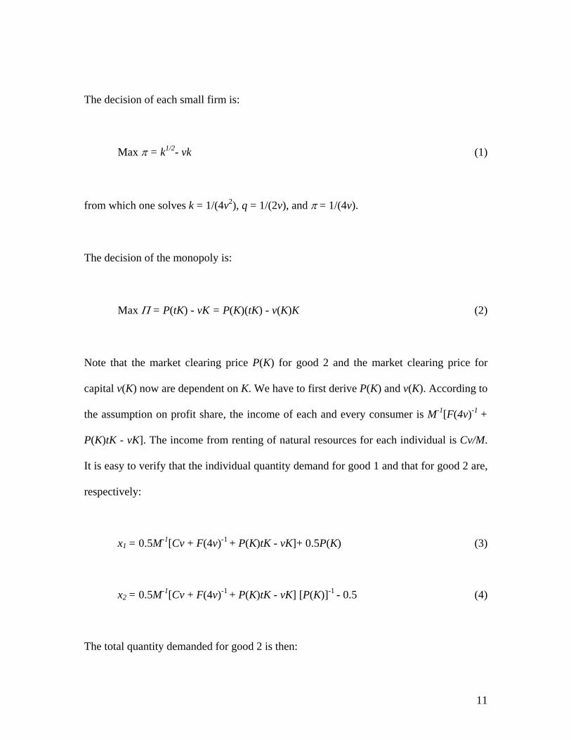
The decision of each small firm is:

Max π = k1/2- vk (1)

from which one solves k = 1/(4v2), q = 1/(2v), and π = 1/(4v).

The decision of the monopoly is:

Max Π = P(tK) - vK = P(K)(tK) - v(K)K (2)

Note that the market clearing price P(K) for good 2 and the market clearing price for

capital v(K) now are dependent on K. We have to first derive P(K) and v(K). According to

the assumption on profit share, the income of each and every consumer is M-1[F(4v)-1 +

P(K)tK - vK]. The income from renting of natural resources for each individual is Cv/M.

It is easy to verify that the individual quantity demand for good 1 and that for good 2 are,

respectively:

x1 = 0.5M-1[Cv + F(4v)-1 + P(K)tK - vK]+ 0.5P(K) (3)

x2 = 0.5M-1[Cv + F(4v)-1 + P(K)tK - vK] [P(K)]-1 - 0.5 (4)

The total quantity demanded for good 2 is then:

12

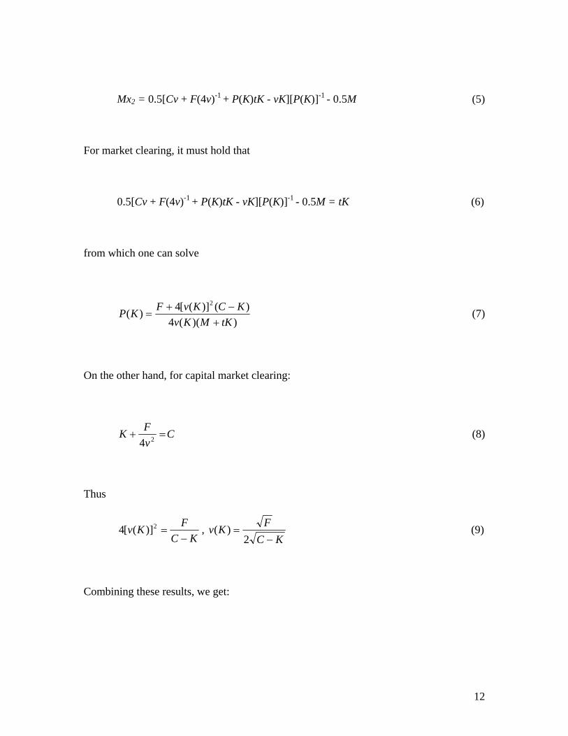
Mx2 = 0.5[Cv + F(4v)-1 + P(K)tK - vK][P(K)]-1 - 0.5M (5)

For market clearing, it must hold that

0.5[Cv + F(4v)-1 + P(K)tK - vK][P(K)]-1 - 0.5M = tK (6)

from which one can solve

))((4)()]([4)(

2

tKMKvKCKvFKP

+−+

= (7)

On the other hand, for capital market clearing:

CvFK =+ 24

(8)

Thus

KCFKv−

=2)]([4 , KC

FKv−

=2

)( (9)

Combining these results, we get:

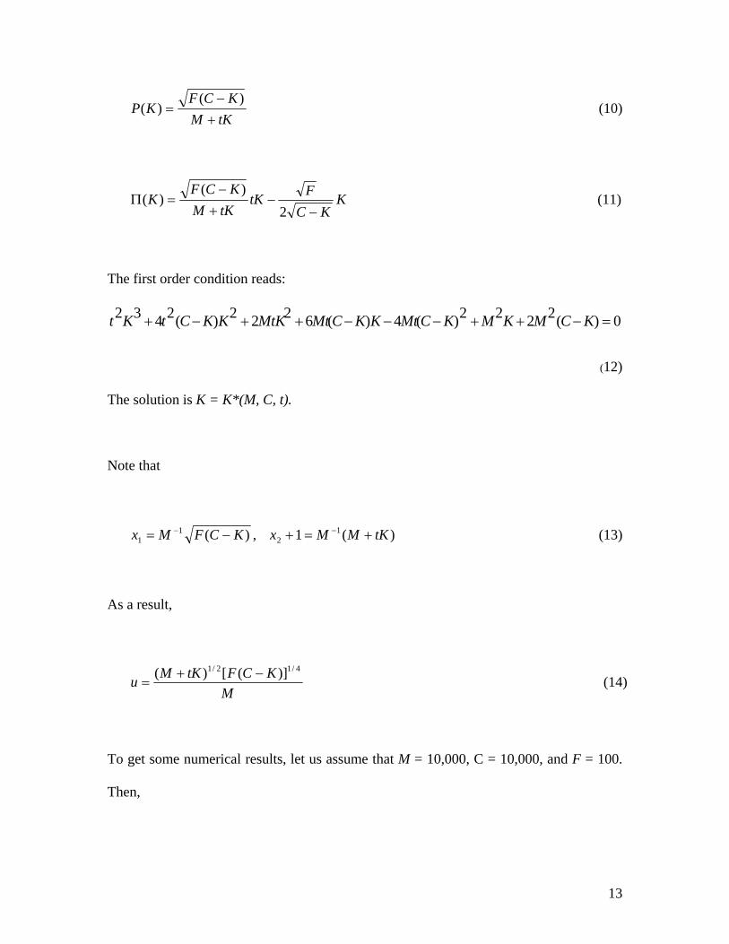
13

tKM

KCFKP

+−

=)(

)( (10)

KKC

FtKtKM

KCFK

−−

+−

=Π2

)()( (11)

The first order condition reads:

0)(2222)(4)(6222)(2432 =−++−−−++−+ KCMKMKCMtKKCMtMtKKKCtKt

(12)

The solution is K = K*(M, C, t).

Note that

)(11 KCFMx −= − , )(1 1

2 tKMMx +=+ − (13)

As a result,

M

KCFtKMu4/12/1 )]([)( −+

= (14)

To get some numerical results, let us assume that M = 10,000, C = 10,000, and F = 100.

Then,

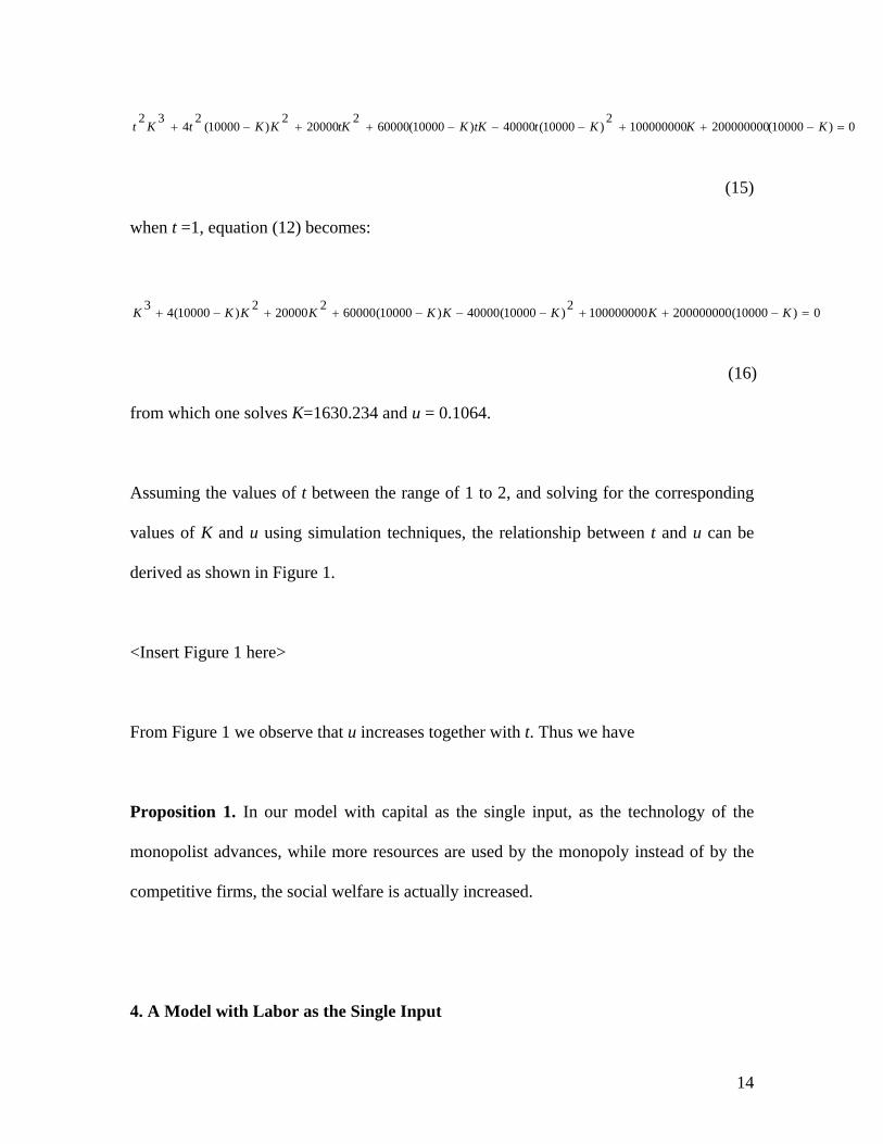
14

0)10000(2000000001000000002

)10000(40000)10000(600002

200002

)10000(2

432

=−++−−−++−+ KKKttKKtKKKtKt

(15)

when t =1, equation (12) becomes:

0)10000(2000000001000000002)10000(40000)10000(600002200002)10000(43 =−++−−−++−+ KKKKKKKKK

(16)

from which one solves K=1630.234 and u = 0.1064.

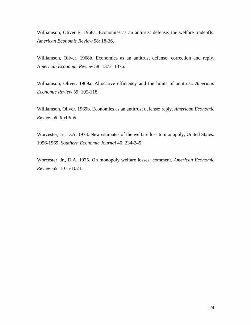
Assuming the values of t between the range of 1 to 2, and solving for the corresponding

values of K and u using simulation techniques, the relationship between t and u can be

derived as shown in Figure 1.

<Insert Figure 1 here>

From Figure 1 we observe that u increases together with t. Thus we have

Proposition 1. In our model with capital as the single input, as the technology of the

monopolist advances, while more resources are used by the monopoly instead of by the

competitive firms, the social welfare is actually increased.

4. A Model with Labor as the Single Input

15

We now consider a model with labor only as the production input. The main difference

between this model and the one in the last section is, consumers’ utilities depend not only

on the consumption amounts of the firms’ products, but also depend on the amounts of

leisure they enjoy.

The economy under consideration consists of one competitive industry and one

monopoly industry as before. Once gain the competitive industry consists of F identical

small firms, of which each produces the same product of good 1, using the same input of

labor, having the same production function q = n1/2, where n is the amount of capital

input. The monopolist produces good 2 with the labor input, and its production function

is Q = tN, where N is the labor input, and t > 0 is a parameter representing the level of

technology.

Once gain there are M identical consumers, each having the same utility function of u =

[Lx1(x2+1)]1/3, where L is the leisure consumed, and xj is the amount of good j consumed.

As before, the utility function implies that good 1 is a necessity, and while the

consumption of good 2 increases the utility from each unit of good 1 consumed, good 2

itself is not a necessity. Each consumer has one unit of time per period used either for

working or for leisure.

Let 1 be the price of good 1, and let w be the wage.

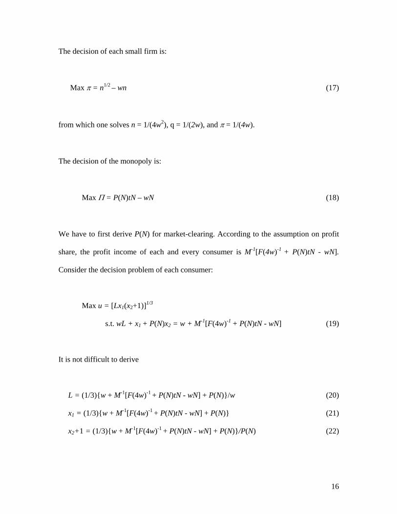
16

The decision of each small firm is:

Max π = n1/2 – wn (17)

from which one solves n = 1/(4w2), q = 1/(2w), and π = 1/(4w).

The decision of the monopoly is:

Max Π = P(N)tN – wN (18)

We have to first derive P(N) for market-clearing. According to the assumption on profit

share, the profit income of each and every consumer is M-1[F(4w)-1 + P(N)tN - wN].

Consider the decision problem of each consumer:

Max u = [Lx1(x2+1)]1/3

s.t. wL + x1 + P(N)x2 = w + M-1[F(4w)-1 + P(N)tN - wN] (19)

It is not difficult to derive

L = (1/3){w + M-1[F(4w)-1 + P(N)tN - wN] + P(N)}/w (20)

x1 = (1/3){w + M-1[F(4w)-1 + P(N)tN - wN] + P(N)} (21)

x2+1 = (1/3){w + M-1[F(4w)-1 + P(N)tN - wN] + P(N)}/P(N) (22)

17

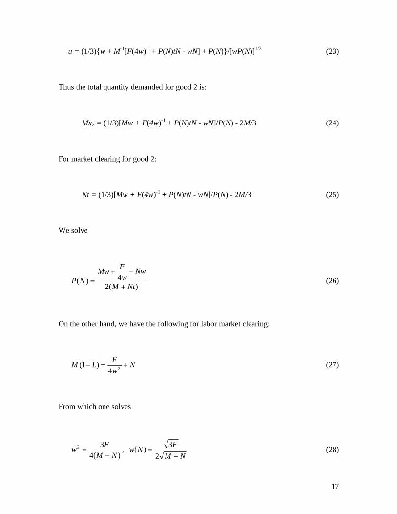
u = (1/3){w + M-1[F(4w)-1 + P(N)tN - wN] + P(N)}/[wP(N)]1/3 (23)

Thus the total quantity demanded for good 2 is:

Mx2 = (1/3)[Mw + F(4w)-1 + P(N)tN - wN]/P(N) - 2M/3 (24)

For market clearing for good 2:

Nt = (1/3)[Mw + F(4w)-1 + P(N)tN - wN]/P(N) - 2M/3 (25)

We solve

)(2

4)(NtM

Nww

FMwNP

+

−+= (26)

On the other hand, we have the following for labor market clearing:

NwFLM +=− 24

)1( (27)

From which one solves

)(4

32

NMFw−

= , NM

FNw−

=2

3)( (28)

18

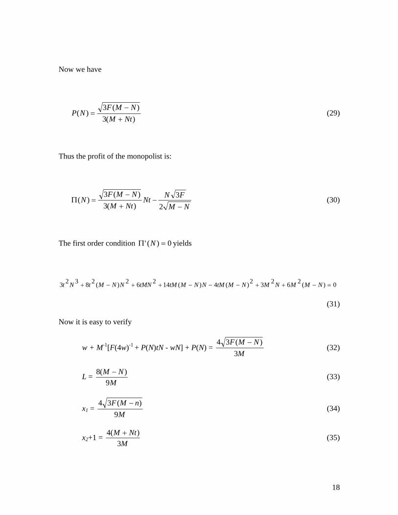
Now we have

)(3

)(3)(

NtMNMF

NP+

−= (29)

Thus the profit of the monopolist is:

NM

FNNtNtM

NMFN

−−

+−

=Π2

3)(3

)(3)( (30)

The first order condition 0)(' =Π N yields

0)(26232)(4)(14262)(28323 =−++−−−++−+ NMMNMNMtMNNMtMtMNNNMtNt

(31)

Now it is easy to verify

w + M-1[F(4w)-1 + P(N)tN - wN] + P(N) = M

NMF3

)(34 − (32)

L = M

NM9

)(8 − (33)

x1 = M

nMF9

)(34 − (34)

x2+1 = M

NtM3

)(4 + (35)

19

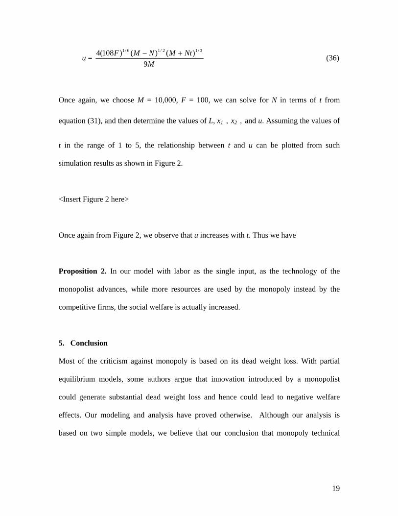
u = M

NtMNMF9

)()()108(4 3/12/16/1 +− (36)

Once again, we choose M = 10,000, F = 100, we can solve for N in terms of t from

equation (31), and then determine the values of L, x1，x2，and u. Assuming the values of

t in the range of 1 to 5, the relationship between t and u can be plotted from such

simulation results as shown in Figure 2.

<Insert Figure 2 here>

Once again from Figure 2, we observe that u increases with t. Thus we have

Proposition 2. In our model with labor as the single input, as the technology of the

monopolist advances, while more resources are used by the monopoly instead by the

competitive firms, the social welfare is actually increased.

5. Conclusion

Most of the criticism against monopoly is based on its dead weight loss. With partial

equilibrium models, some authors argue that innovation introduced by a monopolist

could generate substantial dead weight loss and hence could lead to negative welfare

effects. Our modeling and analysis have proved otherwise. Although our analysis is

based on two simple models, we believe that our conclusion that monopoly technical

20

innovation increases welfare is generally correct. In practice, the development of the

information technology industry, to some extent does justify all our arguments!

Acknowledgements

The authors would like to thank School of Humanities and Social Sciences of Nanyang

Technological University for the research grant (RCC2/2005/SHSS-M52109004) to

conduct this study.

References

Arrow, K. 1962. Economic welfare and the allocation of resources for inventions. In The

rate and direction of inventive activity. Edited by Nelson, R. Princeton: Princeton

University Press.

Bell, Frederic W. 1968. The effect of monopoly profits and wages on prices and

consumers’ surplus in American manufacturing. Western Economic Journal 6: 233-241.

Bergson, Abram. 1973. On monopoly welfare losses, American Economic Review 63:

853-870.

Carson, R. 1975. On monopoly welfare losses: comment. American Economic Review 65:

1008-1014.

Cowling, Keith, and Dennis Mueller. 1978. The social costs of monopoly power.

Economic Journal 88: 727-748.

Delbono, F., and V. Denicolo. 1991. Incentives to innovate in a Cournot oligopoly.

Quarterly Journal of Economics 106: 951-961.

21

DePrano, Michael E., and Jeffery B. Nugent. 1969. Economies as an antitrust defense:

comment. American Economic Review 59: 947-953.

Fellner, W. 1951. The influence of market structure on technological progress. Quarterly

Journal of Economics 65: 556-577.

Friedland, Thomas S. 1978. The estimation of welfare gains from demonopolization.

Southern Economic Journal 45: 116-123.

Geroski, P.A. 1990. Innovation, technological opportunity, and market structure. Oxford

Economic Papers 42: 586-602.

Hansen, Claus Thustrup. 1999. Second-best antitrust in general equilibrium: a special

case. Economics Letters 63: 193-199.

Harberger, A.C. 1954. Monopoly and resource allocation. American Economic Review 44:

77-87.

Hefford, C.B., and David K. Round. 1978. The welfare cost of monopoly in Australia.

Southern Economic Journal 44: 846-860.

Hill, Martyn, and Michael Waterson. 1983. Labor-managed Cournot oligopoly and

industry output. Journal of Comparative Economics 7: 43-51.

Jenny, Frederic, and Andre-Paul Weber. 1983. Aggregate welfare loss due to monopoly

power in the French economy: some tentative estimates. Journal of Industrial Economics

32: 113-130.

Kamerschen, David R. 1966. An Estimation of the welfare losses from monopoly in the

American economy. Western Economic Journal 4: 221-236.

22

Kay, J. A. 1983. A general equilibrium approach to the measurement of monopoly

welfare loss. International Journal of Industrial Organization 1: 317-331.

Kelton, Christina M.L., and Robert P. Rebelein. 2003. A static general-equilibrium model

in which monopoly is superior to competition.

http://irving.vassar.edu/faculty/rr/Research/monopoverCE.pdf (accessed March 16, 2006).

Koo, S.E. 1970. A note on the social welfare loss due to monopoly. Southern Economic

Journal 37: 212-214.

Krueger, Anne. 1974. The political economy of the rent-seeking society. American

Economic Review 64: 291-303.

Lee, Yoon-Ho Alex, and Donald J. Brown. 2005. Competition, consumer welfare, and

the social cost of monopoly. Cowles Foundation Discussion Paper No. 1528.

http://cowles.econ.yale.edu/P/cd/d15a/d1528.pdf (accessed February 4, 2006).

Leibenstein, Harvey. 1966. Allocative efficiency vs. "x-efficiency",” American Economic

Review 56: 392-415.

Littlechild, S.C. 1981. Misleading calculations of the social costs of monopoly power.

Economic Journal 91: 348-363.

Neary, Hugh M. 1984. Labor-managed Cournot oligopoly and industry output: a

comment. Journal of Comparative Economics 8: 322-327.

Neary, Hugh M. 1985. The labor-managed firm in monopolistic competition. Economica

52: 435-447.

Neary, Hugh M. 1992. Some general equilibrium aspects of a labor-managed economy

with monopoly elements. Journal of Comparative Economics 16: 633-654.

23

Parker, R.C., and J.M. Connor. 1979. Estimates of consumer losses due to monopoly in

the U.S. food-manufacturing industries. American Journal of Agricultural Economics 61:

626-639.

Posner, R.A. 1975. The social costs of monopoly and regulation. Journal of Political

Economy 83: 807-828.

Reksulak, Michael, William F. Shughart II, and Robert D. Tollison. 2005. Innovation and

the opportunity cost of monopoly.

http://home.olemiss.edu/~shughart/Innovation%20and%20the%20Opportunity%20Cost

%20of%20Monopoly.pdf (accessed October 20, 2005).

Scherer, Frederic M. 1970. Industrial market structure and economic performance,

Chicago: Rand McNally.

Schwartzman, David. 1960. The burden of monopoly. Journal of Political Economy 68:

627-630.

Shepherd, R.A. 1972. The social welfare loss due to monopoly: comment. Southern

Economic Journal 38: 421-424.

Stigler, George J. 1956. The statistics of monopoly and merger. Journal of Political

Economy 64: 33-40.

Tullock, Gordan. 1967. The welfare costs of tariffs, monopolies, and theft. Western

Economic Journal 5: 224-232.

Waterson, M. 1982. The incentive to invent when a new input is involved. Economica 49:

435-445.

24

Williamson, Oliver E. 1968a. Economies as an antitrust defense: the welfare tradeoffs.

American Economic Review 58: 18-36.

Williamson, Oliver. 1968b. Economies as an antitrust defense: correction and reply.

American Economic Review 58: 1372–1376.

Williamson, Oliver. 1969a. Allocative efficiency and the limits of antitrust. American

Economic Review 59: 105-118.

Williamson, Oliver. 1969b. Economies as an antitrust defense: reply. American Economic

Review 59: 954-959.

Worcester, Jr., D.A. 1973. New estimates of the welfare loss to monopoly, United States:

1956-1969. Southern Economic Journal 40: 234-245.

Worcester, Jr., D.A. 1975. On monopoly welfare losses: comment. American Economic

Review 65: 1015-1023.

25

0.1

0.105

0.11

0.115

0.12

0.125

0.13

1 1.2 1.4 1.6 1.8 2

Level of Technology

Util

ity

Figure 1. Model with Capital as the Single Input: Relationship between the Level of

Technology and Utility

26

0.445

0.45

0.455

0.46

0.465

0.47

0.475

1 1.5 2 2.5 3 3.5 4 4.5 5

Level of technology

Util

ity

Figure 2. Model with Labor as the Single Input: Relationship between the Level of

Technology and Utility