Economic Growth and Public and Private

Investment Returns*

António Afonso # and Miguel St. Aubyn

#

November 2015

Abstract

We study the macroeconomic effects of public and private investment in 17 OECD

economies through a VAR analysis with annual data from 1960 to 2014. From

impulse response functions we find that public investment had a positive growth

effect in most countries, and a contractionary effect in Finland, UK, Sweden, Japan,

and Canada. Public investment led to private investment crowding out in Belgium,

Ireland, Finland, Canada, Sweden, the UK and crowding-in effects in the rest of the

countries. Private investment has a positive growth effect in all countries; crowds-out

(crowds-in) public investment in Belgium and Sweden (in the rest of the countries).

The partial rates of return of public and private investment are mostly positive.

JEL: C32, E22, E62

Keywords: fiscal policy, public investment, private investment, impulse response

functions, VAR

* Preliminary, do not quote without authors’ permission. The opinions expressed herein are those of

the authors and do not necessarily reflect those of their employers. # ISEG/ULisbon – University of Lisbon, Department of Economics; UECE – Research Unit on

Complexity and Economics, R. Miguel Lupi 20, 1249-078 Lisbon, Portugal. UECE is supported by

FCT (Fundação para a Ciência e a Tecnologia, Portugal). Emails: aafonso@iseg.utl.pt;

mstaubyn@iseg.utl.pt.

2

1. Introduction

The 2008-2009 financial and sovereign debt crisis led to a substantial drop in both

GDP and investment levels and growth rates. Moreover, it led to substantial changes

in economic policy, namely budgetary policy. Under budgetary duress, the level of

government indebtedness is deemed to have a negative impact on public investment in

EMU member countries (see, for instance, Turrini, 2004, for the cases in the 1980s

and in the 1990s). In fact, the abovementioned changes took in several countries the

form of reduced expenditure, including public investment, and increased taxation. It is

expectable that these changes may well constitute a policy regime change with

structural implications on previous estimations regarding the relevance of investment

for long-term growth.

Additionally, such policy changes, and especially in countries following

adjustment programs, came with an emphasis on structural reforms that concern

public spending levels and structure, and more generally, the way the economy and

markets operate. It becomes then important to test if macroeconomic efficiency

changes effectively occurred, and in what direction. For instance, Afonso and Jalles

(2015) argue that the relevance of fiscal components differs for private and public

investment developments.

Understanding and measuring linkages between public and private investment and

economic growth are of crucial importance both in developed economies and

emerging markets. Public investment is a part of public expenditure and decisions are

taken within the larger framework of public finance. At the same time, it constitutes

an addition to public capital. The latter, together with private and human capital,

labour and other inputs, is in several approaches considered as a production factor.

Public investment may therefore be linked to growth prospects. However, and as it is

well documented in the literature, as part of public expenditure, it may crowd other

types of investment, namely private, so that in some circumstances the net impact of

public investment on GDP may be negative (see, for instance, Reimers, Dreger, 2014,

Cavalcanti, et al., 2014, IMF, 2014).

At the same time, note the importance of public investment in the fiscal

surveillance mechanisms of the EU, where nº 3 of Article 126 of the Treaty of the

European Union (TEU, 2012) reads:

3

“If a Member State does not fulfil the requirements under one or both of these

criteria, the Commission shall prepare a report. The report of the Commission shall

also take into account whether the government deficit exceeds government

investment expenditure and take into account all other relevant factors, including

the medium-term economic and budgetary position of the Member State”,

which indicates the preference for some Golden Rule based approach for public

investment.

Moreover, the EC (2015) presented a new Investment Plan for Europe in support

of its investment, structural reforms and fiscal responsibility strategy. Once more, the

emphasis on investment is stressed, and a European Fund for Strategic Investments

(EFSI) is created, while it is mentioned that “co-financed expenditure should not

substitute for nationally financed investments, so that total public investments are not

decreased.”

In this paper we contribute to the literature by using a VAR analysis for 17

countries OECD between 1960 and 2014 to assess the effects of public and private

investment in terms of economic growth, crowding out and crowding in effects. In

that context, we also compute public and private investment macroeconomic rates of

return, and assess the potential effect of the 2008 economic and financial crisis, by

comparison with previous shorter time span research, obtained before the crisis.

Our analysis provides notably the following results: public investment had a

positive growth effect in most countries, and a contractionary effect on output in

Finland, UK, Sweden, Japan, and Canada; positive public investment impulses led to

private investment crowding-out in Belgium, Ireland, Finland, Canada, Sweden, the

UK and crowding-in effect on private investment in the rest of the countries; private

investment had a positive growth effect in all countries; private investment crowds-

out public investment in Belgium and Sweden and crowds-in public investment in the

remainder of the countries.

Moreover, the partial rate of return of public investment is mostly positive and the

partial rate of return of private investment is only negative in Greece and marginally

in Belgium.

The paper is organized as follows. In Section 2 we briefly review the literature and

previous results. Section 3 outlines the analytical framework. In Section 4 we present

and discuss our results. Section 5 is the conclusion.

4

2. Literature

There are several techniques and results that allow for crowding in and crowding

out effects of public investment (see Afonso and St. Aubyn, 2009, 2010). Namely,

and within a vector auto regression analysis, different rates of return are estimated.

The total investment rate of return takes into account both private and public

investment costs, while a partial rate of return only considers public investment as

compared to GDP returns.

In Afonso and St. Aubyn (2009, 2010), the extent of crowding in or crowding out

of both components of investment was assessed and the associated macroeconomic

rates of return of public and private investment for each country were computed from

impulse response functions. Results showed the existence of positive effects of public

investment and private investment on output. Crowding in effects of private

investment on public investment were more generalized then the reverse case.

These regularities are likely to be affected by major policy changes after 2009,

namely due to the financial and sovereign debt crisis. In this project we intend to

make further progress in this area of research, namely by studying the impact of the

recent financial and sovereign debt crisis on the linkages between public and private

investment and economic growth.

IMF (2015) documents the private investment contraction in advanced economies

during and after the economic and financial crisis. The “overall weakness of economic

activity” is found to be the most important factor accounting for this shrinking. Our

empirical modelling clearly encompasses this important channel, as private

investment may react contemporaneously and/or with lags to GDP, to public

investment, to taxes and to interest rates.

Some recent research provides evidence that more stringent financial conditions

affect both how the economy reacts to public spending and investment and how

investment responds to the economy. For the specific case of Japan, and using panel

data techniques, Brückner and Tuladhar (2014) show that financial distress has a

significant negative effect on the local government spending multiplier, while

economic slack has a positive effect.

In addition, and in the same vein, but also with a VAR methodology Dreger and

Reimers (2014) refer that, and in what concerns the euro area, public investment

decreases could have adversely affected private investment and GDP. In an interesting

variation, Xu and Yan (2014) study crowding in and crowding out effects in China.

5

They also resort to VAR analysis, and divide public capital formation in investment in

public goods and infrastructure provision and investment involved in the private

goods. Results suggest that the first crowds in private investment while the latter leads

to crowding out.

The reader may also refer to our earlier work for further references on this subject.

Pereira (2000) introduced the estimation of macroeconomic rates of return for

public investment. His VAR-based methodology was further developed by Pina and

St. Aubyn (2005, 2006), who proposed the distinction between a partial and a total-

cost rate of return. This research team, in Afonso and St. Aubyn (2009, 2010),

estimated these rates of return for industrialized countries and also computed private

investment rates of return, and extended previous research by considering a more

complete VAR, by computing confidence bands and by generally presenting more

detailed explanations and results.

3. Analytical framework

The VAR model

We estimate a five-variable VAR model for each country throughout the period

1960-2014 using annual data. As in Afonso and St. Aubyn (2010), where more

detailed explanations may be found, we include five endogenous variables: the

logarithmic growth rates of real public investment, Ipub, real private investment,

Ipriv, real output, Y, real taxes, Tax, and real interest rates, R.

The VAR lag length is determined by the usual information criteria.

The VAR is identified by means of a Cholesky decomposition. Variables are

ordered from the most exogenous variable to the least exogenous one, public

investment being the “most exogenous”. By construction, structural shocks to private

investment, GDP, taxes and the real interest rate affect public investment with a one-

period lag. Private investment responds to public investment in a contemporaneous

fashion, and to shocks to other variables with a lag.

The VAR model in standard form can be written as

1

p

t i t i t

i

X c A X

. (1)

where Xt denotes the (5 1) vector of the five endogenous variables given

by '

log log log logt t t t t tX Ipub Ipriv Y Tax R , c is a (5 1) vector of

6

intercept terms, Ai is the matrix of autoregressive coefficients of order i, and the

vector of random disturbances'

Ipub Ipriv Y Tax R

t t t t t t contains the

reduced form OLS residuals. The lag length of the endogeneous variables, p, will be

determined by the usual information criteria.

Macroeconomic rates of return

We compute four different rates of return: r1, the partial rate of return of public

investment; r2, the rate of return of total investment (originated by an impulse to

public investment); r3, the partial rate of return of private investment; r4, the rate of

return of total investment (originated by an impulse to private investment).

These rates are derived from the VAR impulse response functions, as explained

in Afonso and St. Aubyn (2009). In the following lines we provide the economic

interpretation to these variables.

The partial rate of return of public investment, r1, compares a (partial) cost,

public investment, to a benefit, GDP change, following an impulse to public

investment.

The rate of return of total investment (originated by an impulse to public

investment), r2, compares the total cost (public plus induced private investment), to

the same benefit, GDP change. If more public capital induces more private

investment, we will call this a crowding in case, and r1 will exceed r2. Moreover, if a

positive impulse in public investment leads to a private investment decrease, than r1

will be smaller than r2.

In some cases a positive impulse to public investment will lead to a decrease in

GDP. In those occasions it will not be feasible to compute a rate of return. Note that a

negative rate of return will arise when the benefits, albeit positive, are smaller than

costs.

The rates of return r3 and r4 concern the measurement of consequences to

positive impulses in private investment. As in the case of public investment impulses,

we may have that private investment leads to the crowding in of public investment, or

else that government reacts to private investment impulse by diminishing capital

formation (the crowding out case). In the latter case, r3 will be smaller than r4. The

detailed analytics of the computation of the macroeconomic rates of return are

summarised in Appendix 1.

7

4. Empirical analysis

Data set

We use annual data for 14 EU countries (sample in parenthesis): Austria (1965–

20145), Belgium (1970–2014), Denmark (1971–2014), Germany (1970–2014),

Finland (1961–2014), France (1970–2014), Greece (1973–2014), Ireland (1971–

2014), Italy (1970–2014), the Netherlands (1969–2014), Portugal (1981–2014), Spain

(1979–2014), Sweden (1971–2014), the UK (1970–2014), plus Canada (1964–2004),

Japan (1972–2014), and the United States (1961–2014).

In order to control for the beginning of the 3rd

stage of the Economic and

Monetary Union, and the launching of the euro, on the 1st of January 1999, we have

used a dummy variable that takes the value one from 1999 onwards inclusively. Such

variable is statistically significant in several countries, notably regarding the long-

term interest rate.1

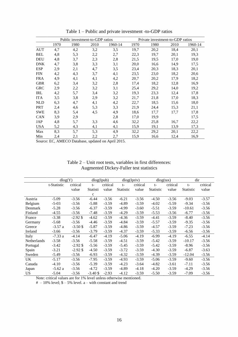
Table 1 summarises the country-specific investment series while Figure 1 plots

the 17 country average private and public investment-to-GDP ratios.

[Table 1]

[Figure 1]

In order to estimate our VAR for each country, we use information for the

following data series: GDP at current market prices; price deflator of GDP; general

government gross fixed capital formation (GFCF) at current prices, used as public

investment; gross fixed capital formation of the private sector at current prices, used

as private investment; taxes (including direct taxes, indirect taxes and social

contributions); nominal long-term interest rate and the consumer price index.

GDP, taxes and investment variables are used in real values using the price

deflator of GDP and the price deflator of the GFCF of the total economy.2 A real ex-

1 To control for the reunification process a dummy was also used for the case of Germany in 1991.

2 Due to the lack of information on a price deflator for private investment, we use the same deflator to

compute both public and private investment variables.

8

post interest rate is computed using the consumer price index inflation rate. All data

are taken from the European Commission Ameco database.3

All variables enter the VAR as logarithmic growth rates, except the interest rate,

where first differences of original values were taken. Moreover, the first differenced

variables are mostly stationary, I (0) time series. Table 2 shows unit root test statistics.

[Table 2]

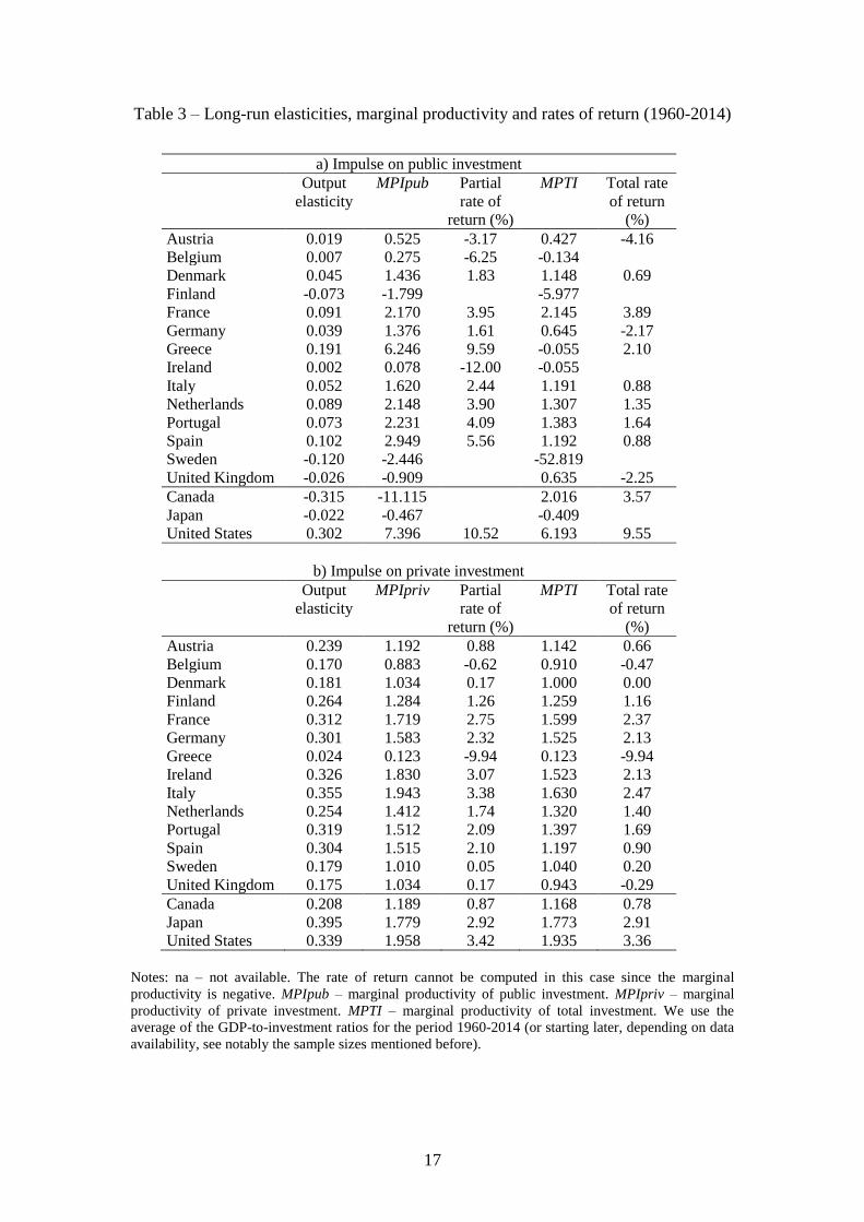
Crowding-out and crowding-in effects

Table 3 summarises the results for the long-run elasticities, the marginal

productivity rates and the macroeconomic rates of return, partial and total, for both

public and private investment for the period 1960-2014 for the 17 country set.

[Table 3]

Figure 2 displays on the vertical axis the marginal effects of public investment

on private investment, allowing the assessment of the existence of crowding-in or

crowding-out effects of public investment on private investment. As Figure 2 shows,

public investment has a positive growth impact in 12 countries and negative one on 5

countries (Finland, UK, Sweden, Japan, and Canada). Moreover, public investment

has a crowding-in effect on private investment in 11 of the 17 countries analysed. Of

the six countries in which public investment crowds-out effect on private investment,

two (Belgium and Ireland) experience a slight output expansion, while Finland,

Canada, Sweden, the UK, show a contractionary effect.

[Figure 2]

[Figure 3]

In a similar way we report in Figure 3 the effects of private investment on output

and the existing crowding-in or crowding-out effects of private investment on public

investment. Moreover, it is also possible to conclude that private investment has an

expansionary effect on output for all 17 countries in the sample. Figure 3 also reveals

3 The data sources are mentioned in Appendix 2.

9

that private investment crowds-in public investment for most countries in the sample,

and crowds-out public investment in the cases of Belgium, and Sweden, This is an

outcome quite in line with the results reported by Afonso and St. Aubyn (2009), for

the period 1960-2004.

Table 4 provides a comparison between the results in this paper, for the period

1960-2014 and the results of Afonso and St. Aubyn (2009) covering the period 1960-

2004. Therefore, the current study encompasses the period of 2008-2009 economic

and financial crisis.

For the cases where such comparison is feasible, Table 4 makes it possible to

draw some additional results, for the period 1960-2014 vis-à-vis the period before the

crisis. Therefore, the total rate of return of public investment increased in three

countries (Portugal, Denmark, and Greece) and decreased in seven countries (Austria,

Germany, Spain, Finland, the UK, Italy and the Netherlands). In addition, the total

rate of return of private investment increased in five countries (Belgium, Germany,

Denmark, France, and Ireland) and decreased in all the other countries but the USA,

where it remained essentially unchanged.

5. Conclusion

In this paper we have used a VAR analysis for 17 countries OECD between 1960

and 2014 to assess the effects of public and private investment in terms of economic

growth, crowding out and crowding in. In that context, we also compute public and

private investment macroeconomic rates of return, and assessed the potential effect of

the 2008 economic and financial crisis.

Our results for the effects of investment shocks show that;

i) public investment had a positive growth effect in most countries;

ii) public investment had a contractionary effect on output in five cases (Finland,

UK, Sweden, Japan, and Canada);

iii) positive public investment impulses led to a decline in private investment

(crowding-out) in six countries (Belgium, Ireland, Finland, Canada, Sweden, the

UK);

iv) public investment had a crowding-in effect on private investment in the

remainder 11 countries;

v) private investment had a positive growth effect in all countries;

10

vi) private investment crowds-out public investment in the cases of Belgium, and

Sweden;

vii) private investment crowds-in public investment in the remainder 15 countries.

Moreover, the partial rate of return of public investment is mostly positive, with

the exceptions of Austria, Belgium, and Ireland, while the total rate of return of public

investment is also negative in Germany and in the UK. On the other hand, the partial

rate of return of private investment is only negative in Greece and marginally in

Belgium, being the total rate of return of private investment negative for Belgium,

Greece, and the UK.

References

Afonso, A., Jalles, J. (2015). “How does fiscal policy affect investment? Evidence

from a large panel”, International Journal of Finance and Economics,

forthcoming.

Afonso, A. and St. Aubyn, M. (2009). “Macroeconomic Rates of Return of Public and

Private Investment: Crowding-in and Crowding-out Effects”, Manchester School,

77 (S1), 21-39.

Afonso, A. and St. Aubyn, M. (2010). “Public and Private Investment Rates of

Return: Evidence for Industrialised Countries”, Applied Economics Letters, 17

(9), 839 - 843.

Brückner, M. and Tuladhar, A (2014). “Local Government Spending Multipliers and

Financial Distress: Evidence from Japanese Prefectures” 124 (581), 1279–1316.

Cavalcanti, C., Merrero, G., Le, T. (2014). “Measuring the Impact of Debt-Financed

Public Investment”, World Bank, Policy Research Working Paper No. 6766.

EC (2015). “Making the best use of the flexibility within the existing rules of the

Stability and Growth Pact”, COM(2015) 12 final, Strasbourg, 13.1.2015,

COM(2015) 12 final.

IMF (2014). “Is it time for an infrastructure push? The macroeconomic effects of

public investment”, IMF World Economic Outlook, October.

Pereira, A. (2000). Is All Public Capital Created Equal? Review of Economics and

Statistics 82 (3), 513-518.

Pina, A. and St. Aubyn, M. (2005). Comparing macroeconomic returns on human and

public capital: An empirical analysis of the Portuguese case (1960–2001).

Journal of Policy Modelling 27, 585-598.

11

Pina, A. and St. Aubyn, M. (2006). How should we measure the return on public

investment in a VAR? Economics Bulletin 8(5), 1-4.

Reimers, H., Dreger, C. (2014). “On the relationship between public and private

investment in the euro area. DIW discussion paper 1365.

TEU (2012). Consolidate version of the Treaty on the functioning of the European

Union, Official Journal of the European Union, 26.10.2012

Turrini, A. (2004). “Public investment and the EU fiscal framework”, European

Economy. European Commission Economic Papers, n°202, May.

Xu, X. and Yan, Y. (2014). “Does government investment crowd out private

investment in China?” Journal of Economic Policy Reform, 17 (1), 1-12.

12

Appendix 1 –The analytics of the macro rates of return

We compute the long-run accumulated elasticity of Y with respect to public

investment, Ipub, from the accumulated impulse response functions (IRF) of the

VAR, as

log

logIpub

Y

Ipub

. (A1)

The long-term marginal productivity of public investment is given by

Ipub

Y YMPIpub

Ipub Ipub

. (A2)

The partial-cost dynamic feedback rate of return of public investment, r1, is the

solution for:

20

1(1 )r MPIpub . (A3)

The long-term accumulated elasticity of Y with respect to Ipriv can also be derived

from accumulated IRF in a similar way:

log

logIpriv

Y

Ipriv

, (A4)

and the long-term marginal productivity of private investment is given by

Ipriv

Y YMPIpriv

Ipriv Ipriv

. (A5)

Therefore, the marginal productivity of total investment, MPTI, is as follows:

1 1

1YMPTI

Ipub Ipriv MPIpub MPIpriv

(A6)

And the rate of return of total investment, from an impulse to public investment, r2, is

the solution for:

MPTIr 20

2 )1( . (A7)

13

Appendix 2 – Data sources

Original series

Ameco codes

Gross Domestic Product at current market prices, thousands national currency. 1.0.0.0.UVGD

Price deflator of Gross Domestic Product, national currency, 1995 = 100.

3.1.0.0.PVGD

Gross fixed capital formation at current prices; general government, national

currency.

1.0.0.0.UIGG

Gross fixed capital formation at current prices; private sector, national

currency.

1.0.0.0.UIGP

Price deflator gross fixed capital formation; total economy, national currency;

1995 = 100.

3.1.0.0.PIGT

Nominal long-term interest rates - % 1.1.0.0.ILN

National consumer price index - 1995 = 100 3.0.0.0.ZCPIN

Current taxes on income and wealth (direct taxes); general government -

National currency, current prices

1.0.0.0.UTYGF;

1.0.0.0.UTYG

Taxes linked to imports and production (indirect taxes); general government -

National currency, current prices

1.0.0.0.UTVGF;

1.0.0.0.UTVG

Social contributions received; general government - National currency, current

prices

1.0.0.0.UTSGF;

1.0.0.0.UTSG

Note: series from the EC AMECO database, April 2015.

14

Figure 1 – Private and public investment-to-GDP ratios, average of all countries

1a – Private investment (% of GDP)

1b – Public investment (% of GDP)

15

Figure 2 – Public investment: marginal productivity (horizontal) and marginal effect

on private investment (vertical), (1960-2014)

Note: AUT – Austria; BEL – Belgium; CAN – Canada; DEU – Germany; DNK – Denmark; ESP – Spain; FIN –

Finland; FRA – France; GBR – United Kingdom; GRC – Greece; IRL – Ireland; ITA – Italy; JAP – Japan; NLD –

Netherlands; PRT – Portugal; SWE – Sweden; USA – United States.

Figure 3 – Private investment: marginal productivity (horizontal) and marginal effect

on public investment (vertical), (1960-2014)

Note: see Figure 2.

16

Table 1 – Public and private investment -to-GDP ratios

Public investment-to-GDP ratios Private investment-to-GDP ratios

1970 1980 2010 1960-14 1970 1980 2010 1960-14

AUT 4,7 4,2 3,2 3,5 19,7 20,2 18,4 20,1

BEL 4,8 5,3 2,2 2,7 22,3 19,7 20,1 19,3

DEU 4,8 3,7 2,3 2,8 21,5 19,5 17,0 19,0

DNK 4,7 3,8 3,3 3,1 20,0 16,6 14,9 17,5

ESP 2,9 2,1 4,7 3,5 23,4 20,3 18,3 20,1

FIN 4,2 4,3 3,7 4,1 23,5 23,0 18,2 20,6

FRA 4,9 4,1 4,1 4,2 20,7 20,2 17,9 18,2

GBR 6,2 3,4 3,2 2,8 17,4 18,2 12,8 16,9

GRC 2,9 2,2 3,2 3,1 25,4 29,2 14,0 19,2

IRL 4,2 5,7 3,4 3,2 19,3 23,3 12,4 17,8

ITA 3,5 3,8 2,9 3,2 21,7 21,8 17,0 18,3

NLD 6,3 4,7 4,1 4,2 22,7 18,5 15,6 18,0

PRT 2,4 4,6 5,3 3,3 21,9 24,4 15,3 21,1

SWE 8,3 5,4 4,5 4,9 18,6 17,7 17,7 17,8

CAN 3,9 2,9 2,8 17,0 19,9 17,5

JAP 4,8 5,7 3,3 4,6 32,2 25,8 16,7 22,2

USA 5,2 4,3 4,1 4,1 15,9 19,1 13,9 17,3

Max 8,3 5,7 5,3 4,9 32,2 29,2 20,1 22,2

Min 2,4 2,1 2,2 2,7 15,9 16,6 12,4 16,9

Source: EC, AMECO Database, updated on April 2015.

Table 2 – Unit root tests, variables in first differences:

Augmented Dickey-Fuller test statistics

dlog(Y) dlog(Ipub) dlog(Ipriv) dlog(tax) dir

t-Statistic critical

value

t-

Statisti

c

critical

value

t-

Statistic

critical

value

t-

Statistic

critical

value

t-

Statistic

critical

value

Austria -5.09 -3.56 -6.44 -3.56 -6.21 -3.56 -4.50 -3.56 -9.03 -3.57

Belgium -5-03 -3.56 -5.88 -3.59 -4.89 -3.59 -4.02 -5.59 -9.34 -3.56

Denmark -5.28 -3.56 -6.37 -3.59 -4.99 -3.60 -5.51 -3.59 -10.61 -3.56

Finland -4.55 -3.56 -7.48 -3.59 -4.29 -3.59 -5.53 -3.56 -6.77 -3.56

France -3.38 -2.92 $ -4.62 -3.59 -4.36 -3.59 -4.41 -3.59 -8.40 -3.56

Germany -5.68 -3.56 -4.46 -3.59 -4.84 -3.59 -5.57 -3.59 -9.35 -3.56

Greece -3.57 a -3.50 $ -5.87 -3.59 -4.86 -3.59 -4.57 -3.59 -7.23 -3.56

Ireland -3.66 -3.56 -3.79 -3.59 -4.37 -3.59 -5.33 -3.59 -6.56 -3.56

Italy -7.33 a -4.14 -6.47 -4.19 -5.06 -4.19 -6.99 -4.19 -6.55 -4.14

Netherlands -3.58 -3.56 -5.58 -3.59 -4.51 -3.59 -5.42 -3.59 -10.17 -3.56

Portugal -3.42 -2.92 $ -5.56 -3.59 -5.45 -3.59 -5.42 -3.59 -8.96 -3.56

Spain -3.21 -2.92 $ -4.50 -3.59 -3.72 -3.59 -4.30 -3.59 -6.87 -3.63

Sweden -5.49 -3.56 -6.93 -3.59 -4.32 -3.59 -4.39 -3.59 -12.04 -3.56

UK -5.17 -3.56 -7.95 -3.59 -4.93 -3.59 -5.06 -3.59 -9.60 -3.56

Canada -4.10 -3.56 -5.39 -3.59 -4.23 -3.64 -4.82 -3.61 -7.11 -3.56

Japan -5.62 a -3.56 -4.72 -3.59 -4.89 -4.18 -4.20 -3.59 -4.29 -3.56

US -5.04 -3.56 -3.40 $ -2.93 -4.12 -3.59 -5.50 -3.59 -7.09 -3.56

Note: critical values are for 1% level unless otherwise mentioned.

# – 10% level; $ – 5% level. a – with constant and trend

17

Table 3 – Long-run elasticities, marginal productivity and rates of return (1960-2014)

a) Impulse on public investment

Output

elasticity

MPIpub Partial

rate of

return (%)

MPTI Total rate

of return

(%)

Austria 0.019 0.525 -3.17 0.427 -4.16

Belgium 0.007 0.275 -6.25 -0.134

Denmark 0.045 1.436 1.83 1.148 0.69

Finland -0.073 -1.799 -5.977

France 0.091 2.170 3.95 2.145 3.89

Germany 0.039 1.376 1.61 0.645 -2.17

Greece 0.191 6.246 9.59 -0.055 2.10

Ireland 0.002 0.078 -12.00 -0.055

Italy 0.052 1.620 2.44 1.191 0.88

Netherlands 0.089 2.148 3.90 1.307 1.35

Portugal 0.073 2.231 4.09 1.383 1.64

Spain 0.102 2.949 5.56 1.192 0.88

Sweden -0.120 -2.446 -52.819

United Kingdom -0.026 -0.909 0.635 -2.25

Canada -0.315 -11.115 2.016 3.57

Japan -0.022 -0.467 -0.409

United States 0.302 7.396 10.52 6.193 9.55

b) Impulse on private investment

Output

elasticity

MPIpriv Partial

rate of

return (%)

MPTI Total rate

of return

(%)

Austria 0.239 1.192 0.88 1.142 0.66

Belgium 0.170 0.883 -0.62 0.910 -0.47

Denmark 0.181 1.034 0.17 1.000 0.00

Finland 0.264 1.284 1.26 1.259 1.16

France 0.312 1.719 2.75 1.599 2.37

Germany 0.301 1.583 2.32 1.525 2.13

Greece 0.024 0.123 -9.94 0.123 -9.94

Ireland 0.326 1.830 3.07 1.523 2.13

Italy 0.355 1.943 3.38 1.630 2.47

Netherlands 0.254 1.412 1.74 1.320 1.40

Portugal 0.319 1.512 2.09 1.397 1.69

Spain 0.304 1.515 2.10 1.197 0.90

Sweden 0.179 1.010 0.05 1.040 0.20

United Kingdom 0.175 1.034 0.17 0.943 -0.29

Canada 0.208 1.189 0.87 1.168 0.78

Japan 0.395 1.779 2.92 1.773 2.91

United States 0.339 1.958 3.42 1.935 3.36

Notes: na – not available. The rate of return cannot be computed in this case since the marginal

productivity is negative. MPIpub – marginal productivity of public investment. MPIpriv – marginal

productivity of private investment. MPTI – marginal productivity of total investment. We use the

average of the GDP-to-investment ratios for the period 1960-2014 (or starting later, depending on data

availability, see notably the sample sizes mentioned before).

18

Table 4 - Marginal productivity and rates of return, 1960-2004 vs 1960-2014

Effect of public investment shock Effect of private investment shock

Marginal

productivity

of public

investment

Marginal

IPUB

effect on

IPRIV

Total rate of

return (with

feedback

effects), %

Marginal

productivity

of private

investment

Marginal

IPRIV

effect on

IPUB

Total rate of

return (with

feedback

effects), %

PRT I 5.18 5.21 -0.9% 1.35 0.16 1.4%

II 2.23 0.61 1.6% 1.51 0.27 0.9%

AUT I 1.60 2.45 -3.8% 1.45 0.07 1.5%

II 0.52 0.23 -4.2% 1.19 0.04 0.7%

BEL I -0.43 -3.02 -7.4% 0.86 -0.03 -0.6%

II 0.27 -3.06 na 0.88 -0.03 -0.5%

DEU I 1.72 0.53 0.6% 1.47 0.03 1.8%

II 1.38 1.13 -2.2% 1.58 0.04 2.1%

DNK I 2.54 1.54 0.0% 0.95 0.04 -0.5%

II 1.44 0.25 0.7% 1.03 0.03 0.0%

FIN I 0.44 0.34 -5.4% 1.06 0.02 0.2%

II -1.80 -0.70 na 1.28 0.02 0.2%

ESP I 2.66 0.72 2.2% 1.56 0.18 1.4%

II 2.95 1.47 0.9% 1.52 0.27 0.9%

FRA I 1.53 -0.56 6.5% 1.35 0.06 1.2%

II 2.17 0.01 3.9% 1.72 0.08 2.4%

GBR I -1.62 -2.03 2.3% 1.84 0.09 2.7%

II -0.91 -2.43 -2.2% 1.03 0.10 -0.3%

GRC I 2.39 1.58 -0.4% 0.91 -0.08 0.0%

II 6.25 3.12 2.1% 0.12 0.00 -9.9%

IRL I -1.60 -2.77 -0.5% 1.85 0.30 1.8%

II 0.08 -2.40 na 1.83 0.20 2.1%

ITA I 0.51 -0.80 4.8% 1.11 -0.34 2.7%

II 1.62 0.36 0.9% 1.94 0.19 2.5%

NLD I -2.72 -2.35 3.6% 1.78 0.07 2.6%

II 2.15 0.64 1.3% 1.41 0.07 1.4%

SWE I 0.13 0.40 -11.3% 1.08 -0.09 0.9%

II -2.45 -0.95 na 1.01 -0.03 0.2%

CAN I -2.31 -2.30 2.9% 1.28 0.03 1.1%

II -11.12 -6.52 3.6% 1.19 0.02 0.8%

JAP I 0.01 -0.99 0.8% 3.09 0.43 3.9%

II -0.47 0.14 na 1.78 0.00 2.9%

USA I 1.83 -2.98 na 2.03 0.06 3.3%

II 7.40 0.19 9.5% 1.96 0.01 3.4%

Notes: I - 1960-2004 (Afonso and St. Aubyn, 2009); II - 1960-2014. na – not available. The rate of

return cannot be computed in this case since the marginal productivity is negative. IPUB – public

investment; IPRIV – private investment. AUT – Austria; BEL – Belgium; CAN – Canada; DEU –

Germany; DNK – Denmark; ESP – Spain; FIN – Finland; FRA – France; GBR – United Kingdom;

GRC – Greece; IRL – Ireland; ITA – Italy; JAP – Japan; NLD – Netherlands; PRT – Portugal; SWE –

Sweden; USA – United States.