economic growth and dynamics of renewable …

Studies in Business and Economics

Studies in Business and Economics - 151 -

ECONOMIC GROWTH AND DYNAMICS OF RENEWABLE

RESOURCE WITH HOUSING, AGRICULTURAL AND RESOURCE LAND USE

ZHANG Wei-Bin Ritsumeikan Asia Pacific University, Japan

Abstract: This paper develops an economic growth model of land use with capital accumulation and dynamics of renewable resource. The economy consists of the industrial, agricultural and renewable resource sectors and the land is distributed among housing, agricultural production and resource growth. The model synthesizes the main ideas in the Solow growth, the Ricardian two-sector economic model, and the logistic model in resource economics in a compact framework. With some specified values of the parameters, we demonstrate that the economic system has a unique equilibrium point. We also conduct comparative dynamic analysis with regard to changes in the industrial sector’s total productivity, the propensities to consume the resource, to consume housing and to save. For instance, our simulation result demonstrates that when the propensity to consume the renewable resource is increased, the land distribution is not affected; both the consumption level and price of the resource are increased; the resource sector increases its output and employs more labor and capital, but the stock of the resource falls over time; the total capital stock and the capital inputs to the agricultural and industrial sectors are reduced; the rate of interest is increased but the wage rate is reduced; less labor is employed by the industrial and agricultural sectors; and the land rent and the price of agricultural good are reduced. Our model also predicts some results different from the growth model with renewable resource by Eliasson and Turnovsky (2004).

Keywords: renewable resource, growth model, economic structure, housing, land distribution 1. Introduction

The loss of forests in association of economic development is observed in many parts of the world. The deforestation has strong impact on biodiversity and climate. Rapid urbanization, wide spread roads and agricultural needs for land make it more expensive to keep land for renewable resources, like forests. Although one can find the deleterious effect of economic development on renewable resources, it is quite challenging to develop a formal theory with interactions among economic growth and dynamics of renewable resources with multiple land uses. The scarcity of natural resources has been introduced into the neoclassical growth theory as early as in the 1970s (e.g., Plourde, 1970, 1971,


- 152 - Studies in Business and Economics

Stiglitz, 1974, Clark, 1976, Dasgupta and Heal, 1979), even though economists had been aware of the necessity of modeling resources with dynamic theory long before. Nevertheless, as pointed out by Munro and Scott (1985), before the 1960s it was quite difficult to develop workable dynamic models of resources. After the 1970s, ome models have been proposed to deal with economic growth with dynamics of environment or/and resources. Nevertheless, it is argued that economics still lacks formal models to properly deal with some basic issues such as dynamic interdependence among land distribution, economic development and renewable resource change are not The purpose of this study is to examine dynamic interactions among economic growth and renewable resources on the basis of the neoclassical growth theory with capital accumulation and renewable resource (e.g., Eliasson and Turnovsky, 2004, Alvarez-Cuadrado and van Long, 2011) with an alternative approach to household behavior.

As far as economic growth mechanism is concerned, the model in this study is based on the neoclassical growth theory. Most of the models in the neoclassical growth theory model are extensions and generalizations of the pioneering works of Solow in 1956.1 The model has played an important role in the development of economic growth theory by using the neoclassical production function and neoclassical production theory. The Solow model has been extended and generalized in numerous directions. The purpose of this study is to integrate the renewable resource and housing with the neoclassical growth theory. The introduction of natural resources into the neoclassical growth theory is addressed by Solow (1999). He argues that if the resource good is used as one of the inputs in the production, then it is easy to incorporate the use of renewable resources into the neoclassical growth model. Nevertheless, an important question is not addressed by Solow. That is, how to incorporate possible consumption of renewable resource into the growth model. There are not many models of growth and renewable resources which treat the renewable resource as a source of utility (see, Beltratti, et al., 1994, Ayong Le Kama, 2001).

This study is not only with renewable resources, but also with land use. Land is an important input to the production of agricultural goods, housing and forest products. Yet, it may be argued that land economics still needs an analytical framework for land distribution with economic structure. It is important to develop an analytical framework in which interactions among economic growth, land distribution, and resource distribution over time can be treated as a consistent manner. For instance, the development of agricultural sector is closely related to the development of other economic sectors and land use distribution is dependent upon the interdependence of different economic sectors. The purpose of this paper is to develop an economic growth model with economic structure and land distribution to explain dynamic interdependence among growth, resource dynamics, sectoral division of labor and capital, and land distribution. The model is an extension of the growth models with renewable resources proposed by Zhang (1995, 2011). In Zhang’s models, land, housing and agricultural product are not

1 The Solow model is sometimes referred as to the Solow-Swan model because Swan (1956) proposed a model similar to the Solow model.



considered at all. This study introduces land distribution, housing and agricultural sector to Zhang’s model. The study is organized as follows. Section 2 defines the basic model. Section 3 shows how we solve the dynamics of the model and simulates the motion of the economic system. Section 4 compares comparative dynamics analysis with regard to changes in the industrial sector’s total productivity, the propensities to consume the resource, to consume housing and to save. Section 5 concludes the study. The appendix proves the main results in Section 3.

2. The Model We are concerned with a national economy without international trade. The

economy consists of industrial, agricultural and renewable sectors. The industrial sector produces industrial goods, which are freely traded in national market. The industrial production is the same as that in the one-sector neoclassical growth model. It is a capital commodity used both for investment and consumption. The agricultural sector produces agricultural goods, which is used for consumption of the population.1 The population is homogenous. The individuals achieve the same utility level regardless of what profession they choose. All the markets are perfectly competitive. We select industrial goods to serve as numeraire.

The industrial sector We assume that production is to combine labor force, ( ),tNi and physical

capital, ( ).tKi We use the conventional production function to describe a relationship

between inputs and output. The production function, ( ),tFi is specified as follows

( ) ( ) ( ) ,1,0,,, =+>= iiiiiiiii AtNtKAtF ii βαβαβα (1)

where ,iA iα and iβ are positive parameters. The production function is a

neoclassical one and homogeneous of degree one with the inputs. Markets are competitive; thus labor and capital earn their marginal products. The rate of interest, ( ),tr

and wage rate, ( ),tw are determined by markets. The marginal conditions are given by

( ) ( )( ) ( ) ( )

( ) ,,tNtFtw

tKtFtr

i

ii

i

iik

βαδ ==+ (2)

1 Agricultural goods are assumed to be consumed simultaneously as they are produced. We neglect possible storage.



where kδ is the given depreciation rate of physical capital.

Agricultural sector We assume that agricultural production is carried out by combination of capital,

( ),tKa labor force, ( ),tNa and land, ( ),tLa as follows

( ) ( ) ( ) ( ) ,1,0,,,, =++>= ςβαςβαςβαaaaaaaaaaa AtLtNtKAtF aa (3)

where ( )tLa is the land employed by the agricultural sector and ,,, aaaA βα

and ς are parameters. The marginal conditions are given by

( ) ( ) ( )( ) ( ) ( ) ( )

( ) ( ) ( ) ( )( ) .,,tL

tFtptRtN

tFtptwtK

tFtptra

aa

a

aaa

a

aaak

ςβαδ ===+ (4)

where ( )tpa is the price of the agricultural good and ( )tR is the land rent.

Change of renewable resources Let ( )tX stand for the stock of the resource.1 The natural growth rate of the

resource is assumed to be a logistic function of the existing stock2

( ) ( )( )( ) ,10

−

tLtXtX

xφφ

where the variable, ( )( ),tLxφ is the maximum possible size for the resource

stock, called the carrying capacity of the resource, and the variable, ,0φ is “uncongested”

or “intrinsic” growth rate of the renewable resource. If the stock is equal to ,φ then the

growth rate should equal zero. If the carrying capacity is much larger than the current stock, then the growth rate per unit of the stock is approximately equal to the intrinsic growth rate. That is, the congestion effect is negligible. In this study, for simplicity we

1 Issues related to modeling management of multiple renewable resource stocks in distinct harvesting grounds and to growth theory with multiple kinds of capital are referred, for instance, for instance, Horan and Shortle (1999), Koundouri and Christou (2006), and Zhang (2005). 2 The logistic model has been frequently used in the literature of growth with renewable resource (e.g., Brander and Taylor, 1997; Brown, 2000; Hannesson, 2000; Cairns and Tian, 2010, Farmer and Bednar-Friedl, 2011). It was proposed early in the nineteenth century. Its wide success in different fields of biological and social sciences is its apparent empirical success. It should be noted that there are some alternative approaches to renewable resources. For instance, Tornell and Velasco (1992), Long and Wang (2009), and Fujiwara (2011) use linear resource dynamics.



assume the intrinsic growth rate constant. This is a strict assumption as the intrinsic rate may change due to changes in other conditions. In this study, we assume that the capacity is dependent on the land used for renewable resources. We require

.0/ ≥xdLdφ If the resource is forest, it is obvious that more land implies high

capacity. In the literature of resource economics, different factors are introduced to make the capacity as an endogenous variable. For instance, in Jinni (2006), the carrying capacity changes as a function of the stock of a renewable resource. See also Benchekroun (2003, 2008) who assumes an inversed-V shaped dynamics of resource accumulation, namely, the resource decreases if its stock is sufficiently large. 1 It should also be mentioned that Munro and Scott (1985), Koskela et al. (2002) and Uzawa (2005: Chap. 2) use more general growth functions in their analysis of renewable resources in growth models. Let ( )tF x stand for the harvest rate of the resource. The change rate in

the stock is then equal to the natural growth rate minus the harvest rate, that is

( ) ( ) ( )( ) ( ).10 tFLtXtXtX xx

−

−=φ

φ (5)

We now examine functional form of the harvest rate. We assume a nationally

owned open-access renewable resource.2 With open access, harvesting occurs up to the point at which the current return to a representative entrant equals the entrant’s cost.3 Aside from the stock of the renewable resources, like the good sector there are two factors of production. We use ( )tNx and ( )tKx to stand for the labor force and capital

stocks employed by the resource sector. We assume that harvesting of the resource is carried out according to the following harvesting production function

( ) ( ) ( ) ( ) ( ) ,1,0,,,,, =+>= xxxxxxxxbx

bxx bbAtNtKtLtXAtF xxx βαβαβα (6)

where xxx bbA α,,, and xβ are parameters. The specified form implies that if

the capital (like machine) and labor inputs are simultaneously doubled, then harvest is

1 With regard to (3), we may consider the capacity dependent on some factors such as efforts. For instance, in the case of forestry fertilizers or cleaning activities of the soil may affect the parameter. With aquaculture, we can also refer to feedings schemes, water temperature, or oxygen levels. See Long (1977), and Levhari and Withagen (1992) for how to introduce human efforts to the dynamics of resources. See also Berck (1981), Ayong Le Kama (2001), and Wirl (2004) for other specifications of renewable resource dynamics. 2 The open-access case was initially examined by Gordon (1954). See Alvarez-Guadrado and VonLong (2011) for recent approaches to growth with renewable resources with different property-rights regimes. 3 This condition may not be satisfied, for instance, when property rights of the resource are incomplete.



also doubled for a given stock of the resource at a given time. It should be noted that the Schaefer harvesting production function which is taken on the following form1

( ) ( ) ( ),tNtXAtF xxx =

is evidently a special case of (6). The Schaefer production function does not take

account of capital (or with capital being fixed). As machines are important inputs in harvesting, we explicitly take account of capital input. Firms choose the capital and labor

inputs in harvesting. We use ( )tpx to denote the price of the resource. The marginal conditions are given as follows

( ) ( ) ( )( ) ( ) ( ) ( )

( ) .,tN

tFtptwtK

tFtptrx

xxx

x

xxxk

βαδ ==+ (7)

Consumer behaviors In this study we use the household’s lot size to stand for housing. Consumers

decide consumption levels of the resource good and commodities, lot size, as well as on how much to save. This study uses the approach to consumers’ behavior proposed by Zhang in the early 1990s. Different from the optimal growth theory in which utility defined over future consumption streams is used, we apply an alternative approach to preference structure of consumers over consumption and saving. We denote per capita wealth by ( ),tk where ( ) ( ) ./ NtKtk ≡ In order to define incomes, it is necessary to determine

land ownership structure. It can be seen that land properties may be distributed in multiple ways under various institutions. This study assumes the absentee land ownership.2 Land is owned by absentee landlords who spend their land incomes outside the economic system. A possible case is that the land is owned by the government and people can rent the land in competitive market. The government uses the income for military or other public purposes. Per capita current income from the interest payment ( ) ( )tktr and the

wage payment ( )tw is given by

( ) ( ) ( ) ( ).twtktrty +=

1 See Schaefer (1957). The function with fixed capital and technology is widely applied to fishing (see also, Paterson and Wilen, 1977). See also Milner-Gulland and Leader-Williams (1992); Bulter and van Kooten (1999). 2 Another two popular assumptions in the literature of land economics are the equally shared landownership and the public ownership. For instance as accepted in Kanemoto (1980), the city government rents the land from the landowners at certain rent and sublets it to households at the market rent, using the net revenue to subsidize city residents equally. Hochman (1981) considers a mixture of absentee and equally shared ownerships. Different ownerships may have different effects on interregional dynamics. The topic about how different land ownerships may affect interregional dynamics will be examined in the future.



We call ( )ty the current income in the sense that it comes from consumers’ daily

work and consumers’ current earnings from ownership of wealth and from the government’s redistribution o the land rent income. The sum of money that consumers are using for consuming and saving are not necessarily equal to the temporary income because consumers can sell wealth to pay, for instance, the current consumption if the temporary income is not sufficient for buying food and touring the country. The total value of wealth that consumers can sell to purchase goods and to save is equal to

( ) ( ),tktpi where ( ) )1(=tpi is the price of the capital good. Here, we assume that

selling and buying wealth can be conducted instantaneously without any transaction cost. The per capita disposable income is given by

( ) ( ) ( ) ( )( ) ( ) ( ).1ˆ twtktrtktyty ++=+= (8)

The disposable income is used for saving and consumption. It should be

remarked that in the growth literature, for instance, in the Solow model, the saving is out of the current income, ,iy while in this study the saving is out of the disposable income

which is dependent both on the current income and wealth. The implications of this approach are similar to those in the Keynesian consumption function and models based on the permanent income hypothesis, which are empirically much more valid than the approaches in the Solow model or the in Ramsey model. The approach to household behavior in this study is discussed at length by Zhang (2005).

At each point of time, a consumer would distribute the total available budget among saving, )(ts , consumption of the commodity, ( ),tc consumption of the resource

good, ( ),tcx consumption of the agricultural good, ( ),tca and the lot size, ( ).tlh The

budget constraint is given by

( ) ( ) ( ) ( ) ( ) ( ) ( ) ( ) ( ).ˆ tytltRtctptctptstc hxxaa =++++ (9)

In our model, at each point of time, consumers have five variables, )(ts , ( ),tc

( ),tcx ( ),tca and ( ),tlh to decide. The consumer’s utility function is specified as follows1

( ) ( ) ( ) ( ) ( ) ( ) ,0,,,,, 0000000000 >= ληχµξληχµξ tstltctctctU hxa

in which ,0ξ ,0µ ,, 00 ηχ and 0λ are the urban household’s elasticity of utility

with regard to the commodity, the agricultural goods, the resource, housing, and saving. 1 Amacher et al. (1999), for instance, introduce fuelwood consumption into the utility function in a study of deforestation. Deacon (1995) assumes that utility level is dependent both on the level of forest services and the extent of the forest that remains standing.



We call ,0ξ ,0µ ,, 00 ηχ and 0λ propensities to consume the commodity, the

agricultural goods, the resource, and housing, and to hold wealth, respectively. Maximizing )(tU subject to the budget constraint (8) yields

,ˆ,ˆ,ˆ,ˆ,ˆ ysylRycpycpyc hxxaa ληχµξ ===== (10)

where

.1,,,,,00000

00000 ληχµξρλρληρηχρχµρµξρξ

++++≡≡≡≡≡≡

The demand for the resource good is given by ./ˆ xx pyc χ= The demand

decreases in its price and increases in the disposable income. An increase in the propensity to consume the resource good increases the consumption when the other conditions are fixed.

Wealth accumulation We now find dynamics of capital accumulation. According to the definition of

( ),ts the change in the household’s wealth is given by

( ) ( ) ( ).tktstk −= (11) The equation simply states that the change in wealth is equal to saving minus

dissaving. Balances of Demand and supply Demand for and supply of the agricultural sector’s output balance at any point of

time

( ) ( ).tFNtc aa = (12)

Demand for and supply of the industrial sector’s output balance at any point of

time

( ) ( ) ( ) ( ) ( ).tKtFtKNtsNtc ik +=++ δ (13)

The demand for and supply of the resource balance at any point of time



( ) ( ).tFNtc xx = (14)

Full employment of the production factors Let N and L stand for respectively the fixed population and land of the

economy. We use ( )tK to stand for the total capital stock. We assume that the total labor

force and capital stock are fully employed by the three sectors. We have

( ) ( ) ( ) ( ),tKtKtKtK xai =++

( ) ( ) ( ) .NtNtNtN xai =++ (15)

The land is also fully used

( ) ( ) ( ) .LtLtLNtl xah =++ (16)

Land use for the resource The land use for residents and agricultural product are determined respectively

by the marginal conditions for the household and the agricultural sector. We now introduce a mechanism to decide the amount of land used for renewable resource. We assume that how much land is kept for the renewable resource is decided by the government. As we assume the public ownership of land, this is possible. We admit that this is a very strict assumption as households may own land and they may use the land to grow the renewable resource. We further assume that there is a stable relationship between the land use for renewable resource and for agriculture. The land of renewable resource is assumed to be

( ) ( ).tLtL ax ϕ= (17)

where ϕ is a constant parameter. This assumption is accepted mainly for

convenience of analysis, it is observed in some economies. For instance, as observed by Ahearn and Alig (2006: 12-13): “The three major uses of land in the contiguous United States are glassland pasture and range, forestland, and cropland. In 1977, these three uses represented 84 percent of all land in the 84 contiguous states. Their respective shares of the total land area have remained remarkably stable over five decades. The share of land in cropland was 24 percent in 24 per cent in 1945 and 1997, with minor variation in the intervening years. The shares of land in forest land and glassland were only slightly less in 1997 than in 1945, 29 compared to 32 per cent and 31 per cent compared to 35 per cent, respectively.” This assumption may be relaxed in two different ways. One is to assume that the government maximizes some social welfare which is related to the land for renewable resource. Another way is to consider ϕ as a function of

the land rents, prices of the resource and agricultural products.



We have thus built the model. We now examine dynamic properties of the model. 3. The dynamics and the motion by simulation This section examines dynamics of the model. First, we introduce a new

variable, ( ) ( ) ( )./ tKtNtz iiii βα≡ We now show that the dynamics can be expressed

by the two-dimensional differential equations system with ( )tz and ( )tX as the

variables. Lemma 1 The motion of the system is determined by the 2 -dimensional differential

equations

( ) ( )[ ] ,ˆ1−

ΛΛ−=

zddzzyz λ

( ) ( ),,10 XzFz

XXX x−

−=Λ=φ

φ (18)

where the functions in (18) are functions of ( )tz and ( )tX determined in the

appendix. Moreover, all the other variables can be determined as functions of ( )tz and

( )tX at any point of time by the following procedure: ( )zk Λ= → NkK = → iK

and aK by (A10) → xK by (A7) → ai NN , and xN by (A1) → iF by (1) → r and w

by (2) → y by (A11) → R by (A12) → ,aL hl and xL by (A14) → xp by (A3) → aF

by (3) → ap by (4) → acc, and s by (10).

The differential equations system (18) contains two variables ( )tz and ( ).tX

Lemma 1 shows that once we determine the values of the two variables with some initial conditions, we can determine all the variables in the economic system. The lemma is important as it gives a procedure to follow the motion of the system with computer with a given initial condition.

It should be noted that the land distribution is constant over time given as

follows



,,,1 axaha LLLl

NLL ϕηηϕ

==++

=

where ./ µςηη ≡ The constant land distribution is due to the specified Cobb-

Douglas production and utility functions as well as the competitive land markets and the proportional relationship between the agricultural and resource land use. Relaxation of any of these assumptions may lead to non-constant land distribution. It is straightforward to show that a rise in the proportional parameter, ,ϕ reduces the land for the agricultural

production and housing. A rise in the propensity to consume housing, ,η increases the

lot size and reduces the land use for the agricultural production and the resource. A rise in the propensity to consume the agricultural good, ,µ or in the share of the total cost of the

agricultural production to the land rent, ,ς reduces the lot size and increases the land use

for the agricultural production and the resource. A steady state of (18) is determined by ( ) ( ) ,0ˆ =Λ− zzyλ

( ) ( ) .0,10 =−

− XzF

zXX xφ

φ

As the expressions of the analytical results are tedious, for illustration we

specify the parameter values and simulate the model. We specify the capacity function as

( ) .0, ≥= xxxxLL θθφ θ

This implies that as more land is distributed the renewable resource, the

capacity is increased (in the case of .xθ If ,0=xθ then the capacity is constant. If

,1=xθ the capacity is proportional to the land size. We specify the parameters as

follows

,2.0,1.0,5.0,3.0,1,3.0,10,5 ======== aaaxii AALN βααα

,01.0,02.0,07.0,5.0,8.0,9.0,3,5.0 00000 ======== ηχξλθθφ xxA



.05.0,01.0,7.0,5,6.1,02.00 0 ====== kxbb δφϕµ (19)

The adjustment speed, ,0φ is fixed at .3 The power parameter, ,xθ in the

capacity function implies that the capacity exhibits decreasing return to the land. As the land, for instance, for forest is doubled, the capacity of forestation may less be doubled. This may happen, for instance, more land may be used for road construction for logging. We assume that the propensity to save is much higher than the propensity to consume the commodity and the propensity to consume the renewable resource. Some empirical studies on the US economy demonstrate that the value of the parameter,

,α in the Cobb-Douglas production is approximately equal to 3.0 (for instance, Miles and

Scott, 2005, Abel et al, 2007). The land for resource use is 6.1 times as much as the land for agricultural use. With regard to the technological parameters, what are important in our study are their relative values.

Under (16), the dynamic system has a unique equilibrium point. The

equilibrium values of the variables are given as follows

,24.0,94.3,59.1,87.0,21.7,81.2,95.37 ======= aixai NNFFFXK

,023.0,83.4,02.3,24.6,08.2,63.29,83.0 ======= rLLKKKN xaxaix

,06.1,43.0,59.7,96.0,74.1,35.0,283.1 ======= clkppRw hxa

,32.0,18.0 == xa cc

The two eigenvalues are 27.4− and .14.0− This guarantees the stability of

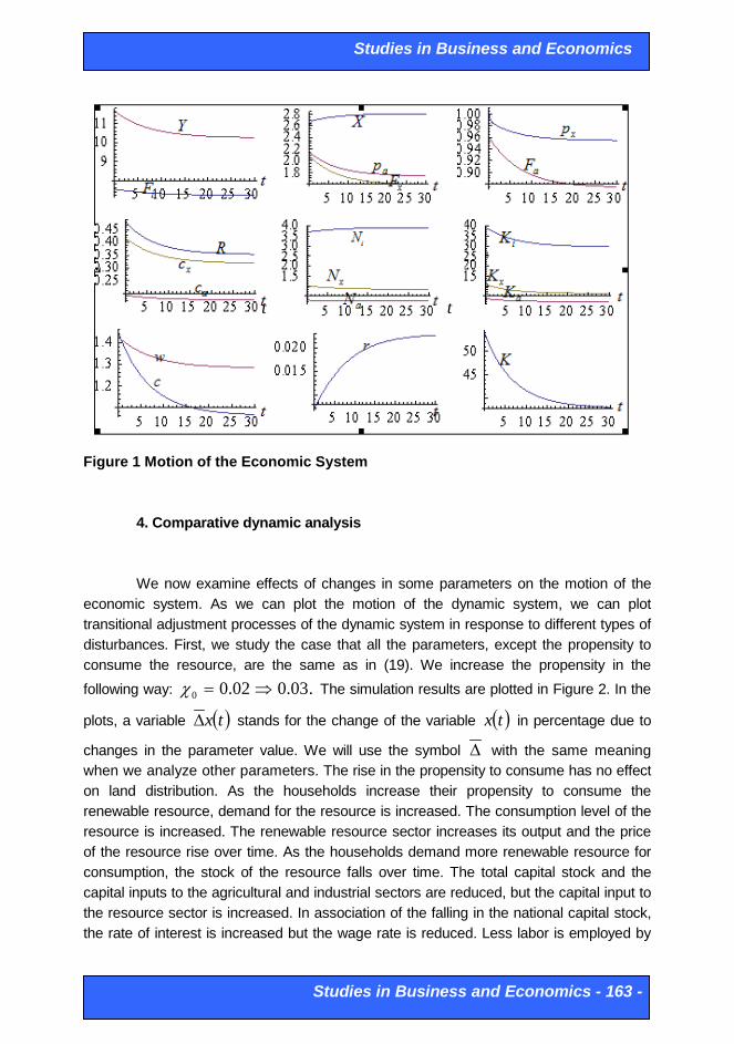
the steady state. Hence, the dynamic system has a unique stable steady state. With the initial conditions, ( ) 04.00 =z and ( ) ,6.20 =X we plot the motion of the system as in Figure 1. The national capital stock at the initial state is much higher than its equilibrium value and the stock of the resource at the initial state is lower than its equilibrium value. The period length of the simulation is long enough for the whole system to achieve its steady state. We see that the level of the resource stocks rises over time till it achieves its long-term steady value. Correspondingly the price of the resource falls. The total capital is reduced over time and the rate of interest is increased over time. The capital stocks employed by and outputs of the three sectors fall over time. The labor input employed by the resource sector and the agricultural sector fall slightly and the labor input employed by the industrial sector rises over time. The wage rate and consumption levels of the three goods fall over time.



Figure 1 Motion of the Economic System

4. Comparative dynamic analysis We now examine effects of changes in some parameters on the motion of the

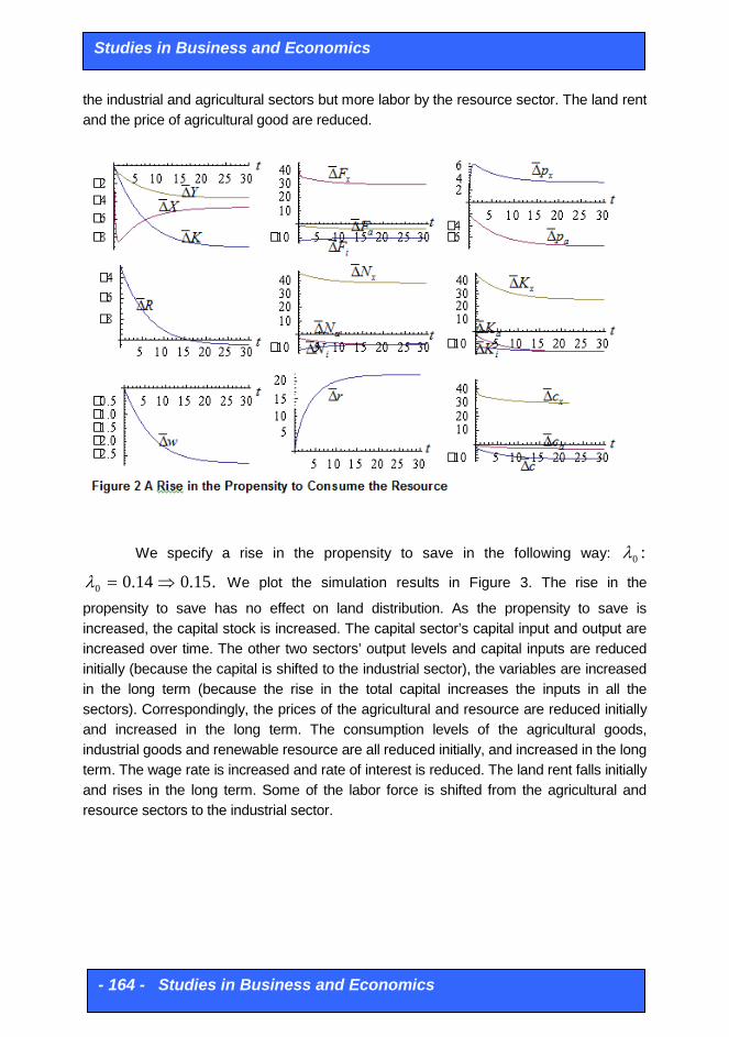
economic system. As we can plot the motion of the dynamic system, we can plot transitional adjustment processes of the dynamic system in response to different types of disturbances. First, we study the case that all the parameters, except the propensity to consume the resource, are the same as in (19). We increase the propensity in the following way: .03.002.00 ⇒=χ The simulation results are plotted in Figure 2. In the

plots, a variable ( )tx∆ stands for the change of the variable ( )tx in percentage due to

changes in the parameter value. We will use the symbol ∆ with the same meaning when we analyze other parameters. The rise in the propensity to consume has no effect on land distribution. As the households increase their propensity to consume the renewable resource, demand for the resource is increased. The consumption level of the resource is increased. The renewable resource sector increases its output and the price of the resource rise over time. As the households demand more renewable resource for consumption, the stock of the resource falls over time. The total capital stock and the capital inputs to the agricultural and industrial sectors are reduced, but the capital input to the resource sector is increased. In association of the falling in the national capital stock, the rate of interest is increased but the wage rate is reduced. Less labor is employed by

t t



the industrial and agricultural sectors but more labor by the resource sector. The land rent and the price of agricultural good are reduced.

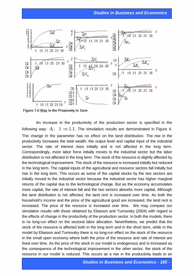
We specify a rise in the propensity to save in the following way: :0λ

.15.014.00 ⇒=λ We plot the simulation results in Figure 3. The rise in the

propensity to save has no effect on land distribution. As the propensity to save is increased, the capital stock is increased. The capital sector’s capital input and output are increased over time. The other two sectors’ output levels and capital inputs are reduced initially (because the capital is shifted to the industrial sector), the variables are increased in the long term (because the rise in the total capital increases the inputs in all the sectors). Correspondingly, the prices of the agricultural and resource are reduced initially and increased in the long term. The consumption levels of the agricultural goods, industrial goods and renewable resource are all reduced initially, and increased in the long term. The wage rate is increased and rate of interest is reduced. The land rent falls initially and rises in the long term. Some of the labor force is shifted from the agricultural and resource sectors to the industrial sector.



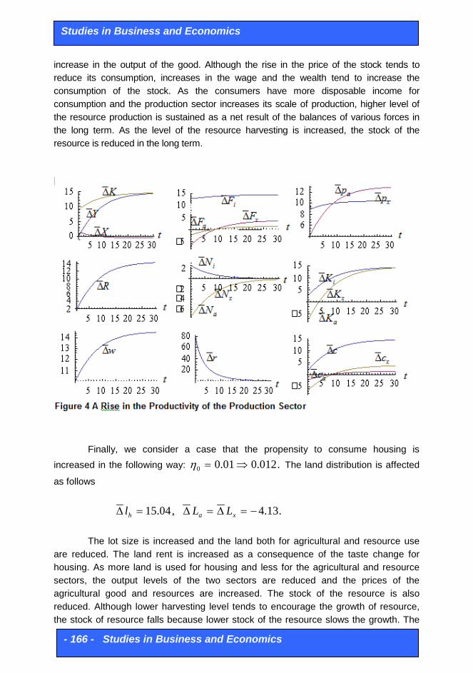
An increase in the productivity of the production sector is specified in the following way: :iA .1.11 ⇒ The simulation results are demonstrated in Figure 4.

The change in the parameter has no effect on the land distribution. The rise in the productivity increases the total wealth, the output level and capital input of the industrial sector. The rate of interest rises initially and is not affected in the long term. Correspondingly, more labor force initially moves to the industrial sector but the labor distribution is not affected in the long term. The stock of the resource is slightly affected by the technological improvement. The stock of the resource is increased initially but reduced in the long term. The capital inputs of the agricultural and resource sectors fall initially but rise in the long term. This occurs as some of the capital stocks by the two sectors are initially moved to the industrial sector because the industrial sector has higher marginal returns of the capital due to the technological change. But as the economy accumulates more capital, the rate of interest fall and the two sectors absorbs more capital. Although the land distribution is not affected, the land rent is increased over time. As both the household’s income and the price of the agricultural good are increased, the land rent is increased. The price of the resource is increased over time. We may compare our simulation results with those obtained by Eliasson and Turnovsky (2004) with regard to the effects of change in the productivity of the production sector. In both the models, there is no long-run effect on the sectoral labor allocation. Nevertheless, we predict that the stock of the resource is affected both in the long term and in the short term, while in the model by Eliasson and Turnovsky there is no long-run effect on the stock of the resource in the small open economy where both the price of the resource and rate of interest are fixed over time. As the price of the stock in our model is endogenous and is increased as the consequence of the technological improvement in the other sector, the stock of the resource in our model is reduced. This occurs as a rise in the productivity leads to an



increase in the output of the good. Although the rise in the price of the stock tends to reduce its consumption, increases in the wage and the wealth tend to increase the consumption of the stock. As the consumers have more disposable income for consumption and the production sector increases its scale of production, higher level of the resource production is sustained as a net result of the balances of various forces in the long term. As the level of the resource harvesting is increased, the stock of the resource is reduced in the long term.

Finally, we consider a case that the propensity to consume housing is

increased in the following way: .012.001.00 ⇒=η The land distribution is affected

as follows

,04.15=∆ hl .13.4−=∆=∆ xa LL

The lot size is increased and the land both for agricultural and resource use

are reduced. The land rent is increased as a consequence of the taste change for housing. As more land is used for housing and less for the agricultural and resource sectors, the output levels of the two sectors are reduced and the prices of the agricultural good and resources are increased. The stock of the resource is also reduced. Although lower harvesting level tends to encourage the growth of resource, the stock of resource falls because lower stock of the resource slows the growth. The



capital inputs to the agricultural and resource sectors fall initially but rise in the long term. The rise of the propensity to consume housing also implies reduction of the propensities to save and to consume the industrial goods. A fall in the propensity to save tends to reduce the national capital stocks, but a fall in the propensity to consume the industrial good tends to increase the national capital. Moreover, the higher inputs of both labor and capital in the industrial sector tend to increase the national capital stocks. The net consequence of the different forces results in a rise in the national capital. This also implies why in the long term all the three sectors employ more capital as a consequences of the taste change.

6. Concluding Remarks This study proposed a growth model with renewable resource by synthesizing the

main ideas in the two key models in the neoclassical growth theory and resource economics. We also model land-use distribution in an economy with the industrial, agricultural and renewable resource sectors. By simulation, we demonstrated that the economic system has a unique equilibrium point. We also conducted comparative dynamic analysis with regard to changes in the industrial sector’s total productivity, the propensities to consume the resource, to consume housing and to save. Our model also predicts some results different from the growth model with renewable resource by Eliasson and Turnovsky (2004). We limit our study to a simplified structure of the economic system. Many limitations of this model become apparent in the light of the



sophistication of the literature of growth theory, agricultural economics and resource economics. The Solow model is the key model in the neoclassical economic growth theory and the logistic model is the key model in the dynamics of resource economics. Numerous meaningful extensions of either of the two models have already existed. We may also generalize our model, for instance, by using more general production and utility functions, or by introducing more realistic representations of housing market dynamics.

Appendix: Proving Lemma 1 The appendix shows that the dynamics can be expressed by two-dimensional

differential equations. From (2), (4) and (7), we obtain

,~~~

x

xx

a

aa

i

iik

KN

KN

KN

wrz αααδ

===+

≡ (A1)

where we omit time index and ,/~

jjj βαα ≡ .,, xaij = By (1) and (2), we

have

,~

,~ i

ii

i zAwzAr iii

i

iik α

αβ

ββα

ααδ ==+ (A2)

where we also use (A1). We can express w and r as functions of .z From (6)

and (7), we solve

,~ x

x zLXArp x

bx

bxx

kx

βαα

δ

+= (A3)

where we also use (A1). Hence xp is a function of zX , and .xL From (14)

and (10), we get

.ˆ xx FpyN =χ (A4)

From (12) and (10), we get

.ˆ aa FpNy =µ (A5)

From (4) and (7), we have



.x

xxx

a

aaak K

FpK

Fpr ααδ ==+ (A6)

Substituting (A4) and (A5) into (A6) yields

,0 ax KK α= (A7)

where ./0 µαχαα ax≡ Insert (A1) in NNNN xai =++

.~~~ NzKKKx

x

a

a

i

i =

++ααα

(A8) Insert (A8) in KKKK xai =++ and (A8)

( ) ,1 0 KKK ai =++ α ,~ 1 zNKK

ai

i =+ αα

(A9)

where .~/~/1 01 xa αααα +≡ Solve (A9) with iK and aK as the variables

( )

,~,100

01 β

αβ

αα

−=

+

−=i

aiK

zNK

zNKK (A10)

where

( ) .~/11

010

iαααβ

+−≡

By (A10) and (A7), we solve the capital distribution, ai KK , and ,xK as

functions of z and .K By (A1), we solve the labor distribution, ai NN , and ,xN as

functions of z and .K From (A4) and (7), we have



.ˆN

Nwyx

x

χβ= (A11)

Hence, y is a function of z and .K By (4) and (A5), we have

.ˆ

aLNyR µς

= (A12)

From hlyR /ˆη= in (10) and (A12), we have

.ah Ll η= (A13)

From (16), (17) and (A13), we solve the land distribution follows

.,,1 axaha LLLl

NLL ϕηηϕ

==++

= (A14)

The land distribution is invariant over time. From (A12), we solve R a function of

z and .K Insert (10) and (1) in (13)

( ) ,ˆ KNKAyN iiiii δλξ βα +=+ (A15)

where .1 kδδ −≡ From (A1) and (A15) we have

( ) ,~ˆ KKAzyN iii

i

δα

λξβ

+

=+ (A16)

Insert (A11) in (A16)

( ) ( ) ,KKzKz iiaa δφφ += (A17)

where we also use ,~/ xxx KzN α= ax KK 0α= and



( ) ( ) ( ) .~,~0

ii

ixx

a Azzzwziβ

αφ

χβααλξφ

≡

+≡

From (A17) and (A10), we solve k as a function of z

( ) ( )( ) .11~ 0

1

01 z

zk iai

ai φαφ

βδ

αφ

φα ++

++≡Λ=

−

(A18)

It is straightforward to check that all the variables (except X and z ) can be

expressed as functions of X and z at any point of time. It is straightforward to see that the right-hand side of (5) is a function of ( )tz and ( ).tX Hence, we have

( ) ( ),, XztX Λ=

where we do explicitly express ( )Xz ,Λ as it straightforward but its expression is tedious.

Taking derivatives of (A18) with respect to t yields

.zzd

dk Λ= (A19)

From (8) and (9), we have

( ) .ˆ kzyk −= λ (A20) From (A20) and (A21), we solve

( ) ( )[ ] ,ˆ1−

ΛΛ−=

zddzzyz λ (A21)

where we also use (A18). We have thus proved Lemma 1.



7. References

Amacher, G.S., Hyde, W.F., and Kanel, K.R. (1999) Nepali Felwood Production and Consumption: Regional and Household Distinctions, Substitution and Successful Intervention. Journal of Development Studies 35, 138-63.

Ahearn, M.C. and Alig, R.J. (2006) A Discussion of Recent Land-Use Trends, in Economics of Rural Land-Use Change, edited by Bell, K.P., Boyle, K.L., and Rubin, J. Aldershot: Ashgate.

Deacon, R.T. (1995) Assessing the Relationship between Government Policy and Deforestation. Journal of Environmental Economics and Management 28, 1-18.

Abel, A., Bernanke, B.S., and Croushore, D. (2007) Macroeconomics. New Jersey: Prentice Hall. Ayong Le Kama, A.D. (2001) Sustainable Growth, Renewable Resources and Pollution. Journal of

Economic Dynamics and Control 25, 1911-18. Alvarez-Guadrado, F. and von Long, N. (2011) Consumption and Reneable Resource Extraction

under Alternative Property-Rights Regimes. Resource and Energy Economics (forthcoming).

Azariadis, C. (1993) Intertemporal Macroeconomics. Oxford: Blackwell. Beltratti, A., Chichilnisky, G., and Heal, G.M. (1994) Sustainable Growth and the Golden Rule, in

The Economics of Sustainable Development, edited by Goldin, I. and Winters, I.A. Cambridge: Cambridge University Press.

Benchekroun, H. (2003) Unilateral Production Restrictions in a Dynamic Duopoly. Journal of Economic Theory 111, 237-61.

Berck, P. (1981) Optimal Management of Renewable Resources with Growing Demand and Stock Externalities. Journal of Environmental Economics and Management 11, 101-18.

Brander, J.A. and Taylor, M.S. (1998). The Simple Economics of Easter Island: A Ricardo-Malthus Model of Renewable Resource Use. American Economic Review, 81, 119-38.

Brown, G.M. (2000) Renewable Natural Resource Management and Use Without Markets. Journal of Economic Literature 38, 875-914.

Bulter, E.H. and Van Kooten, G.C. (1999) Economics of Antipoaching Enforcement and the Ivory Trade Ban. American Journal of Agricultural Economics 81, 453-66.

Cairns, D.R. and Tian, H.L. (2010). Sustained Development of a Society with a Renewable Resource. Journal of Economic Dynamics & Control, 24, 2048-61.

Clark, C.W. (1976) Mathematical Bioeconomics: The Optimal Management of Renewable Resources. New York: Wiley.

Dasgupta, P.S. and Heal, G.E. (1979) The Economics of Exhaustible Resources. Cambridge: Cambridge University Press.

Eliasson, L. and Turnovsky, S.J. (2004) Renewable Resources in an Endogenously Growig Economy: Balanced Growth and Transitional Dynamics. Journal of Environmental Economics and Management 48, 1018-49.

Farmer, K. and Bednar-Friedl, B. (2010) Intertemporal Resource Economics – An Introduction to the Overlapping Generations Approach. New York: Springer.

Fujiwara, K. (2011) Losses from Competition in a Dynamic Game Model of a Renewable Resource Oligopoly. Resource and Energy Economics 33, 1-11.

Gordon, H.S. (1954) The Economic Theory of a Common Property Resource: The Fishery. Journal of Political Economy, 62, 124-42.

Hannesson, R. (2000). Renewable resources and the gains from trade. Canadian Journal of Economics, 33, 122-32.



Hochman, O. (1981) Land Rents, Optimal Taxation and Local Fiscal Independence in an Economy with Local Public Goods. Journal of Public Economics 15, 59-85.

Horan, R. and Shortle, J. (1999) Optimal Management of Multiple Renewable Resource Stocks: An Application to Minke Whales. Environmental and Resource Economics 23, 45-58.

Jinji, N. (2006) International Trade and Terrestrial Open-Access Renewable Resources in a Small Open Economy. Canadian Journal of Economics 39, 790-808.

Kanemoto, Y. (1980) Theories of Urban Externalities. Amsterdam: North-Holland. Koskela, E., Ollikainen, M., and Puhakka, M. (2002) Renewable Resources in an Overlapping

Generations Economy Without Capital. Journal of Environmental Economics and Management 43, 497-517.

Koundouri, P. and Christou, C. (2006) Dynamic Adaptation to Resource Scarcity and Backstop Availability: Theory and Application to Grounwater. Australian Journal of Agricultural and Resource Economics 50, 227-45.

Levhari, D. and Withagen, C. (1992) Optimal Management of the Growth Potential of Renewable Resources. Journal of Economics 56, 297-309.

Long, N.V. and Wang, S. (2009) Resource-grabbing by Status-conscious Agents. Journal of Development Economics 89, 39-50.

Miles, D. and Scott, A. (2005) Macroeconomics – Understanding the Wealth o Nations. Chichester: John Wiley & Sons, Ltd.

Milner-Gulland, E.J. and Leader-Williams, N. (1992) A Model of Incentives for the Illegal Exploitation of Black Rhinos and Elephants. Journal of Applied Ecology 29, 388-401.

Munro, G.R. and Scott, A.D. (1985) The Economics of Fisheries Management, in Handbook of Natural Resource and Energy Economics, vol. II, edited by Kneese, A.V. and Sweeney, J.L., Amsterdam: Elsevier.

Paterson, D.G. and Wilen, J.E. (1977). Depletion and Diplomacy: The North-Pacific Seal Hunt, 1880-1910. In Uselding, P. (Ed.), Research in Economic History. JAI Press.

Plourde, G.C. (1970) A Simple Model of Replenishable Resource Exploitation. American Economic Review 60, 518-22.

Plourde, G.C. (1971) Exploitation of Common-Property Replenishible Resources. Western Economic Journal 9, 256-66.

Schaefer, M.B. (1957). Some Considerations of Population Dynamics and Economics in Relation to the Management of Marine Fisheries. Journal of Fisheries Research Board of Canada 14, 669-81.

Solow, R. (1956) A Contribution to the Theory of Growth. Quarterly Journal of Economics 70, 65-94. Solow, R. (1999) Neoclassical Growth Theory, in Handbook of Macroeconomics, edited by Taylor,

J.B. and Woodford, M. North-Holland. Stiglitz, J.E. (1974) Growth with Exhaustible Natural Resources: Efficient and Optimal Growth

Paths. Review of Economic Studies, Symposium on the Economics of Exhaustible Resources, 123-38.

Swan, T.W. (1956) Economic Growth and Capital Accumulation. Economic Record 32, 334-61. Tornell, A. and Velasco, A. (1992) The Tragedy of the Commons and Economic Growth: Why

does Capital Flow from Poor to Rich Countries? Journal of Political Economy 100, 1208-31.

Uzawa, H. (2005) Economic Analysis of Social Common Capital. Cambridge: Cambridge University Press.

Wirl, F. (2004) Sustainable Growth, Renewable Resources and Pollution: Thresholds and Cycles. Journal of Economic Dynamics & Control 28, 1149-57.



Zhang, W.B. (1995) Growth with Renewable Resources. Umeå Economic Studies No. 367, University of Umeå.

Zhang, W.B. (2005) Economic Growth Theory. Hampshire: Ashgate. Zhang, W.B. (2008) International Trade Theory: Capital, Knowledge, Economic Structure, Money

and Prices over Time and Space. Berlin: Springer. Zhang, W.B. (2011) Renewable Resources, Capital Accumulation, and Economic Growth.

Business Systems Research (forthcoming)

economic growth and dynamics of renewable …

Documents