http://edq.sagepub.com/Economic Development Quarterly

http://edq.sagepub.com/content/early/2013/10/21/0891242413506610The online version of this article can be found at:

 DOI: 10.1177/0891242413506610

published online 18 October 2013Economic Development QuarterlyJason P. Brown, Stephan J. Goetz, Mary C. Ahearn and Chyi-lyi (Kathleen) Liang

Linkages Between Community-Focused Agriculture, Farm Sales, and Regional Growth  

- Feb 19, 2014version of this article was published on more recent A

Published by:

http://www.sagepublications.com

can be found at:Economic Development QuarterlyAdditional services and information for    

  http://edq.sagepub.com/cgi/alertsEmail Alerts:

 

http://edq.sagepub.com/subscriptionsSubscriptions:  

http://www.sagepub.com/journalsReprints.navReprints:  

http://www.sagepub.com/journalsPermissions.navPermissions:  

What is This? 

- Oct 18, 2013OnlineFirst Version of Record  

- Oct 28, 2013OnlineFirst Version of Record >>  

- Feb 19, 2014Version of Record

at UNIV OF MICHIGAN on April 12, 2014edq.sagepub.comDownloaded from at UNIV OF MICHIGAN on April 12, 2014edq.sagepub.comDownloaded from

Economic Development QuarterlyXX(X) 1 –12© The Author(s) 2013Reprints and permissions: sagepub.com/journalsPermissions.navDOI: 10.1177/0891242413506610edq.sagepub.com

Article

Introduction

U.S. agricultural output nearly tripled from 1948 to 2009 on roughly the same farm land base1 (U.S. Department of Agriculture, Economic Research Service [USDA, ERS], 2012b). In 2007, three quarters of all output was produced by about 125,000 farms, accounting for 5.7% of all farms (U.S. Department of Agriculture, National Agricultural Statistics Service [USDA, NASS], 2009). The success of the agricul-tural sector is increasingly associated with concerns about secondary impacts that flow from the organization and pro-duction of the agricultural and food system. Concerns include lower food quality and safety, greater environmental degra-dation, and depopulation of some rural areas due to a large farm structure. These consumer sentiments have likely con-tributed to the increasing interest in local foods among U.S. consumers that is at the core of the U.S. Department of Agriculture’s (USDA) “Know Your Farmer, Know Your Food” initiative (USDA, 2012). “Know Your Farmer, Know Your Food” was established in 2009 to coordinate and high-light activities and authorized programs of USDA agencies focused on promoting local and regional food systems.

The imbalance in the farm size and farm sales distribution has posed at least two important questions. First, how are farm enterprises with a greater community orientation contributing to agricultural and regional growth? Second, with production con-centrated on few farms and with labor-saving technologies con-tributing to the productivity gains in agriculture, how important is agriculture in the economic growth of a region? We label

on-farm enterprises that keep economic activity in the local community as community-focused agriculture (CFA). In our analysis, CFA includes sales of farm commodities directly to consumers and farm income from agritourism.

Local markets are believed to provide farmers with a higher share of the food dollar, with money spent at a local farm and nonfarm businesses circulating within the community, creat-ing a multiplier effect and providing greater local economic benefits (USDA, 2012). Furthermore, agritourism generates additional dollars in the local economy as visitors spend money in associated regional travel. As a result, CFA is seen as a potential contributor to local economic growth. However, little empirical research documents the linkages between CFA, or agriculture more broadly, and regional growth.

This study seeks to help fill the gap in the literature by examining the county-level linkages between CFA and growth in total agricultural sales with overall personal income growth in the county. Our study is motivated in part by the continuing debate (e.g., Carlin & Saupe, 1993; Hayes & Olmstead, 1984) about the Goldschmidt (1946) hypothesis

506610 EDQXXX10.1177/0891242413506610Economic Development Quarterly XX(X)Brown et al.research-article2013

1Federal Reserve Bank of Kansas City, Kansas City, MO, USA2The Pennsylvania State University, University Park, PA, USA3USDA Economic Research Service, Washington, DC, USA4University of Vermont, Burlington, VT, USA

Corresponding Author:Jason P. Brown, Federal Reserve Bank of Kansas City, 1 Memorial Drive, Kansas City, MO 64198, USA. Email: jason.brown@kc.frb.org

Linkages Between Community-Focused Agriculture, Farm Sales, and Regional Growth

Jason P. Brown1, Stephan J. Goetz2, Mary C. Ahearn3, and Chyi-lyi (Kathleen) Liang4

AbstractCommunity-focused agriculture has been heralded as a development strategy to induce local economic growth. This study examines county-level linkages between community-focused agriculture and growth in total agricultural sales and economic growth more broadly. Using Census of Agriculture data, regional growth models are estimated on real personal income per capita change between 2002 and 2007. We find no association between community-focused agriculture and growth in total agricultural sales at the national level, but do in some regions of the United States. A $1 increase in farm sales led to an annualized increase of $0.04 in county personal income. With few exceptions, community-focused agriculture did not make significant contributions to economic growth in the time period analyzed.

Keywordsregional growth, farm structure, community-focused agriculture

at UNIV OF MICHIGAN on April 12, 2014edq.sagepub.comDownloaded from

2 Economic Development Quarterly XX(X)

linking county economic well-being to the size distribution of farms. Although we do not explicitly investigate the farm size distribution here, our principal measure of agricultural activity—growth in total farm sales in a county—strongly reflects the underlying local distribution of farms.

The Agricultural Supply Chain and Community-Focused Agriculture

Farmers make on-farm production and management choices with knowledge of their targeted supply chain, including knowledge of the demands of the final consumer for particu-lar product attributes. Farm products in a supply chain are transferred through three main channels: (a) spot markets, the traditional channel, which transmit price signals to buyers and sellers; (b) vertical integration where the farm production unit is part of a larger firm that moves the farm product to the next step in the firm’s supply chain; and (c) preproduction contracts between a farmer (usually operating a large farm) and the next stage in the supply chain. Currently, marketing and production contracts account for about 40% of the value of U.S. agricultural production (USDA, ERS, 2012a).

Farm products with a transparent “locally grown” brand-ing are moving through all the traditional supply chain mod-els. For example, farmers markets are a type of spot market eliminating the “middle man,” a local winery that produces its own grapes and labels the product as locally grown is a form of vertical integration, and Wal-Mart’s contracting with small, local farmers to purchase vegetables to be branded and mar-keted as local is an example of local farm products moving through traditional channels. In addition, new channels are developing that are specifically tailored to meet consumer demand, presumably more efficiently, for local foods in the form of local and regional food hubs (Barham et al., 2012).

The 2007 Census of Agriculture reports that only 136,817 or 6.2% of all farms sold commodities for human consump-tion (i.e., excluding products such as hay, Christmas trees, or ornamentals).2 Since these farms are more likely to be small, their direct sales represent less than 1% of all sales (whether or not nonfood products are excluded). The 2007 count rep-resents an increase from 2002, when only 116,733 farms reported direct sales. Local food activities are relatively more important to New England states. For example, although 6.2% of all farms reported having direct sales to individuals in 2007, 21.6% did in the New England States.

In fact, for the past three decades the Census of Agriculture reports that a small share of farms have engaged in direct sales, from a low of 4.2% in 1997 to a high of 6.4% in 1982. An annual sample survey of farms, the Agricultural and Resource Management Survey (ARMS), shows some increase in farms engaged in direct sales since 2007—exceeding 10% of farms in some years (Ahearn, 2012). This is consistent with significant growth in the number of farm-ers markets across the country to 7,864 in 2012, compared

with 4,685 as recently as 2008 (U.S. Department of Agriculture, Agricultural Marketing Service, 2012).

In addition to selling farm products directly to consumers, some farmers sell products through a very short supply chain directly to a local retail outlet that brands the product as local. For example, this includes sales to restaurants or local retail stores that perhaps purchased the products through a local food hub and market them as local. To distinguish these from direct-to-consumer sales, they are labeled as sales to intermediaries (King et al., 2010). Direct sales to intermedi-aries were first collected on the 1998 ARMS (and never on the Census of Agriculture) and the share of farms engaged in these types of sales has been very low, 3% to 4%.3 Low and Vogel (2011) documented the extent of local food sales in 2008, including sales by farms to intermediaries who sold directly to consumers. Based on ARMS data, most farms engaged in local food sales sold directly to the consumer, such as at farmers’ markets, but a larger share of the value of local foods sales was marketed through intermediaries.

Farmers in certain regions also generate community-focused farm revenues by providing agritourism goods and services. Demand for local foods coupled with the apprecia-tion of farmland amenities has contributed to the demand for farm recreational visits, such as u-pick operations and agri-tourism. Farm recreation activities, in turn, contribute to more market activity in the broader local community. Farms engaged in agritourism enterprises are even less common than those engaged in direct sales.4 In 2007, 23,350 farms (1.1% of all farms) nationally reported income from farm recreational activities, down from 28,016 in 2002.

Farm families engaged in community-focused farm enter-prises market goods and services through multiple channels, besides directly to consumers. They are more likely to be smaller than other farms. Consistent with their size distribu-tion relative to other farms, they earn less on the farm and more likely lose money farming on a cash basis (after depre-ciation). Most U.S. family farms lose money from farming in a typical year because most are small, with most production concentrated on a small share of large farms. There are many reasons small farms stay in operation despite farm losses, but one common explanation is that the farm provides other types of returns such as asset appreciation and a dwelling. Most families operating small farms rely on off-farm income for support. Still others find success in market niches, such as CFA enterprises. In general, just as the linkages of small- and medium-sized farms to their local communities afford them off-farm work opportunities, links to local communi-ties are key to succeeding in CFA enterprises.

Agricultural Linkages to Economic Growth

The successes of U.S. agricultural exports are in part the result of high rates of productivity growth and reductions in

at UNIV OF MICHIGAN on April 12, 2014edq.sagepub.comDownloaded from

Brown et al. 3

the use of farm labor over time. The share of U.S. jobs in farming is now less than 2%—and less than 6% in nonmetro counties. Of course, agricultural labor requirements vary over regions, depending on commodities and many other factors. The farm economy is closely tied to the world econ-omy because of extensive trade in agricultural commodities.5 Although agriculture’s exports have been a positive force in the U.S. macro economy, its ties to the global economy have made it vulnerable to periods of slow world growth or a strong U.S. dollar. In testing export base theory, Kilkenny and Partridge (2009) found that across all U.S. counties dur-ing the decade of the 1990s, counties with high concentra-tions of export activities (i.e., mining, agriculture, and manufacturing) had lower employment growth.

Agricultural impacts on local economies are likely to vary with the structure of the local agriculture, such as the size distribution of the farms and the commodity mix. For exam-ple, bulk commodities have a smaller proportional effect on the nonfarm economy than processed or high-value com-modities (USDA, ERS, 2012c). Evidence also exists to sug-gest that large farms are less likely to purchase their farm inputs locally (Foltz, Jackson-Smith, & Chen, 2002; Foltz & Zeuli, 2005) and that where farm households purchase farm inputs and household consumables varies by region (Lambert, Wojan, & Sullivan, 2009). Conversely, farm households that operate off-farm businesses have been shown to have strong links to the local nonfarm economy in rural areas (Vogel, 2012).

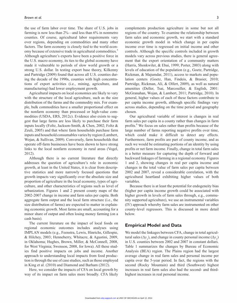
Although there is no current literature that directly addresses the question of agriculture’s role in economic growth, at least in the United States, it is clear from descrip-tive statistics and more narrowly focused questions that growth impacts vary significantly over the absolute size and proportion of agriculture in the local economy, types of agri-culture, and other characteristics of regions such as level of urbanization. Figures 1 and 2 present county maps of the 2002-2007 change in income and farm sales per capita. Both aggregate farm output and the local farm structure (i.e., the size distribution of farms) are expected to matter in explain-ing economic growth. Most farms are small, accounting for a minor share of output and often losing money farming (on a cash basis).

The current literature on the impact of local foods on regional economic outcomes includes analyses using IMPLAN models (e.g., Feenstra, Lewis, Hinrichs, Gillespie, & Hilchey, 2003; Henneberry, Whitacre, & Agustini, 2009, in Oklahoma; Hughes, Brown, Miller, & McConnell, 2008, for West Virginia; Swenson, 2008, for Iowa). All these stud-ies find positive impacts on jobs and income. Another approach to understanding local impacts from food produc-tion is through the use of case studies, such as those employed in King et al. (2010) and Diamond and Barham (2012).

Here, we consider the impacts of CFA on local growth by way of its impact on farm sales more broadly. CFA likely

complements production agriculture in some but not all regions of the country. To examine the relationship between farm sales and economic growth, we start with a standard economic growth model in which change in per capita income over time is regressed on initial income and other controls. Although the specific controls included in growth models vary across previous studies, there is general agree-ment that the export orientation of a community matters (Harris, Shonkwiler, & Ebai, 1999; Porter, 2003) along with levels of education of the population (e.g., Goetz, Partridge, Rickman, & Majumdar, 2011), access to markets and popu-lation centers (Goetz, Han, Findeis, & Brasier, 2010; Partridge, Rickman, Ali, & Olfert, 2009), as well as natural amenities (Deller, Tsai, Marcouiller, & English, 2001: McGranahan, Wojan, & Lambert, 2011; Partridge, 2010). In general, higher values of each of these factors contribute to per capita income growth, although specific findings vary across studies, depending on the time period and geography chosen.

Our agricultural variable of interest is changes in real farm sales per capita in a county rather than changes in farm profits.6 We focus on sales rather than profits because of the large number of farms reporting negative profits over time, which could make it difficult to detect any effects. Furthermore, farm profits are part of county income, and as such we would be estimating portions of an identity by using profits or net farm income. Finally, change in total farm sales is a better measure for capturing the depth of forward and backward linkages of farming in a regional economy. Figures 1 and 2, showing changes in real per capita income and changes in the total value of farm sales per capita between 2002 and 2007, reveal a considerable correlation, with the agricultural heartland exhibiting higher values of both variables.

Because there is at least the potential for endogeneity bias (higher per capita income growth could be associated with higher growth in levels of farm sales through, e.g., commu-nity supported agriculture), we use an instrumental variables (IV) approach whereby farm sales are instrumented on other county-level regressors. This is discussed in more detail below.

Empirical Model and Data

We model the linkages between CFA, change in total agricul-tural sales (Δy

1), and change in county personal income (Δy

2)

in U.S. counties between 2002 and 2007 in constant dollars. Table 1 summarizes the changes by Bureau of Economic Analysis (BEA) region. The Plains region had the largest average change in real farm sales and personal income per capita over the 5-year period. In fact, the regions with the second (Rocky Mountain) and third (Southwest) highest increases in real farm sales also had the second- and third-highest increases in real personal income.

at UNIV OF MICHIGAN on April 12, 2014edq.sagepub.comDownloaded from

4 Economic Development Quarterly XX(X)

This raises the possibility that increases in farm sales over this period could have been an independent driver of eco-nomic growth in some regions of the country. To test this hypothesis, we specify Equations (1) and (2), which are esti-mated simultaneously by IV two-stage least squares.

∆y1 = f(share of profitable farms,

community-focused agriculture), (1)

∆y2 = f(∆y

1, base income, export orientation,

human capital, market access, natural amenities). (2)

Standard tests are used to determine the strength, valid-ity, and necessity of using the IV model compared with a more efficient (but possibly inconsistent) single-stage model estimated by ordinary least squares. These include tests for

weak instruments, overidentification, and exogeneity of the presumed endogenous regressor. The weak instrument F test investigates whether the instruments are sufficiently corre-lated with the endogenous variable to avoid large biases. The value of the test statistic can be compared with thresh-old values for different levels of bias as shown by Stock and Yogo (2005). The overidentification test investigates the hypothesis that the IV are valid (i.e., exogenous—not cor-related with the error term in the model—and valid to exclude from the main equation being estimated). The exo-geneity test investigates whether the potentially endogenous regressor is exogenous (a rejection implies that it is not). Rejection of this last hypothesis (together with passing the first two tests for the validity of the IV model) supports the IV model as the best model, whereas failure to reject sup-ports the use of the more efficient single-stage model (Wooldridge, 2002).

Figure 1. Change in real personal income per capita, 2002 to 2007.Source. Constructed by the authors.

at UNIV OF MICHIGAN on April 12, 2014edq.sagepub.comDownloaded from

Brown et al. 5

Table 2 shows the empirical measures used in the growth equations. An indicator of initial conditions using the level of personal income per capita in 2002 (pci

02) is included to

account for growth trajectories over the study period (e.g., Harris, 2011; Isserman & Rephann, 1995; White & Hanink, 2004). Export orientation of county industry is measured using the share of business establishments that are in trad-able sectors (tradable).7 Human capital in a county is mea-sured using the percentages of the adult population with associate’s, bachelor’s, and master’s degrees (Rupasingha, Goetz, & Freshwater, 2002). Market access as well as urban influence are controlled for by using miles of interstate highways (interstate) in the county and travel times to urban population centers of 25,000 (dt25k), 250,000 (dt250k), and 1,000,000 (dt1000k) people (Monchuk,

Table 1. County Average Change in Real Personal Income and Farms Sales (2002 to 2007)a.

Region

Average change in real personal

income (per capita)

Average change in real farm sales

(per capita)

New England 2720.58 56.55Mideast 2539.37 137.96Great Lakes 850.28 752.91Plains 3422.09 5059.32Southeast 1893.46 336.98Southwest 3004.69 1392.56Rocky Mountain 3731.92 1499.53Far West 2629.16 377.14

Source. BEA, REIS; 2002 and 2007 Census of Agriculture USDA, NASS.

Figure 2. Change in real farm sales per capita, 2002 to 2007.Source. Constructed by the authors.

at UNIV OF MICHIGAN on April 12, 2014edq.sagepub.comDownloaded from

6 Economic Development Quarterly XX(X)

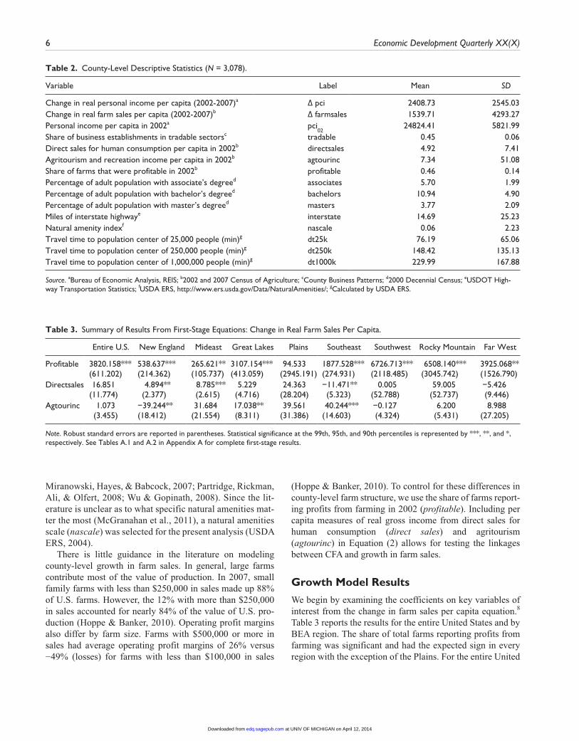
Table 3. Summary of Results From First-Stage Equations: Change in Real Farm Sales Per Capita.

Entire U.S. New England Mideast Great Lakes Plains Southeast Southwest Rocky Mountain Far West

Profitable 3820.158*** (611.202)

538.637*** (214.362)

265.621** (105.737)

3107.154*** (413.059)

94.533(2945.191)

1877.528*** (274.931)

6726.713*** (2118.485)

6508.140***(3045.742)

3925.068** (1526.790)

Directsales 16.851(11.774)

4.894**(2.377)

8.785*** (2.615)

5.229(4.716)

24.363(28.204)

−11.471** (5.323)

0.005(52.788)

59.005 (52.737)

−5.426(9.446)

Agtourinc 1.073(3.455)

−39.244**(18.412)

31.684 (21.554)

17.038** (8.311)

39.561(31.386)

40.244*** (14.603)

−0.127(4.324)

6.200 (5.431)

8.988(27.205)

Note. Robust standard errors are reported in parentheses. Statistical significance at the 99th, 95th, and 90th percentiles is represented by ***, **, and *, respectively. See Tables A.1 and A.2 in Appendix A for complete first-stage results.

Table 2. County-Level Descriptive Statistics (N = 3,078).

Variable Label Mean SD

Change in real personal income per capita (2002-2007)a Δ pci 2408.73 2545.03Change in real farm sales per capita (2002-2007)b Δ farmsales 1539.71 4293.27Personal income per capita in 2002a pci

0224824.41 5821.99

Share of business establishments in tradable sectorsc tradable 0.45 0.06Direct sales for human consumption per capita in 2002b directsales 4.92 7.41Agritourism and recreation income per capita in 2002b agtourinc 7.34 51.08Share of farms that were profitable in 2002b profitable 0.46 0.14Percentage of adult population with associate’s degreed associates 5.70 1.99Percentage of adult population with bachelor’s degreed bachelors 10.94 4.90Percentage of adult population with master’s degreed masters 3.77 2.09Miles of interstate highwaye interstate 14.69 25.23Natural amenity indexf nascale 0.06 2.23Travel time to population center of 25,000 people (min)g dt25k 76.19 65.06Travel time to population center of 250,000 people (min)g dt250k 148.42 135.13Travel time to population center of 1,000,000 people (min)g dt1000k 229.99 167.88

Source. aBureau of Economic Analysis, REIS; b2002 and 2007 Census of Agriculture; cCounty Business Patterns; d2000 Decennial Census; eUSDOT High-way Transportation Statistics; fUSDA ERS, http://www.ers.usda.gov/Data/NaturalAmenities/; gCalculated by USDA ERS.

Miranowski, Hayes, & Babcock, 2007; Partridge, Rickman, Ali, & Olfert, 2008; Wu & Gopinath, 2008). Since the lit-erature is unclear as to what specific natural amenities mat-ter the most (McGranahan et al., 2011), a natural amenities scale (nascale) was selected for the present analysis (USDA ERS, 2004).

There is little guidance in the literature on modeling county-level growth in farm sales. In general, large farms contribute most of the value of production. In 2007, small family farms with less than $250,000 in sales made up 88% of U.S. farms. However, the 12% with more than $250,000 in sales accounted for nearly 84% of the value of U.S. pro-duction (Hoppe & Banker, 2010). Operating profit margins also differ by farm size. Farms with $500,000 or more in sales had average operating profit margins of 26% versus −49% (losses) for farms with less than $100,000 in sales

(Hoppe & Banker, 2010). To control for these differences in county-level farm structure, we use the share of farms report-ing profits from farming in 2002 (profitable). Including per capita measures of real gross income from direct sales for human consumption (direct sales) and agritourism (agtourinc) in Equation (2) allows for testing the linkages between CFA and growth in farm sales.

Growth Model Results

We begin by examining the coefficients on key variables of interest from the change in farm sales per capita equation.8 Table 3 reports the results for the entire United States and by BEA region. The share of total farms reporting profits from farming was significant and had the expected sign in every region with the exception of the Plains. For the entire United

at UNIV OF MICHIGAN on April 12, 2014edq.sagepub.comDownloaded from

Brown et al. 7

States, a 1% increase in the share of farms reporting profits would have been associated with an increase in farm sales per capita of $3,820 between 2002 and 2007. This effect ranged from $538 per capita in New England to $6,726 per capita in the Rocky Mountain region. Clearly, profitability in earlier time periods induces more production from farms, but the response differs by region.

There was no evidence of positive or negative linkages between CFA and growth in farm sales nationally; how-ever, the associations differed significantly across regions of the country. Increases from the 2002 level of direct sales for human consumption were associated with increases in farm sales in New England and Mideast counties. One dollar increase from the 2002 level was associated with nearly a $5 and $9 increase in total farm sales in those regions. Given the proximity to large urban populations in these regions, it is reasonable to assume that the local food dollar was spread around more in the food supply chain. Direct sales were negatively associated with changes in farm sales in Southeastern counties, with a $1 increase reducing total farm sales by $11. One possible explanation is that local food distribution channels are not as well developed in this region of the country relative to New England and the Mideast. This requires further investiga-tion, which is beyond the scope of the present analysis.

Agritourism income appears to be a substitute to produc-tion agriculture in the New England region. A $1 increase from the 2002 per capita level of agritourism income was associated with a decrease in total farm sales per capita of $39 over the study period. Conversely, increases in agritour-ism income were positively associated with increases in total farm sales in Great Lakes and Southeast counties. In these areas, a $1 increase in agritourism income was associated with increases of $17 and $40 in total farm sales between 2002 and 2007.

We now turn to results from the personal income growth equation. Regression results for the entire nation (all coun-ties included) are reported in Table 4. An F test on the excluded instruments from the first-stage equation (profit-able, directsales, agtourinc) rejects that the instruments are weak. The test statistic value of 13.53 is sufficiently larger than the critical value of 9.08 identified by the Stock–Yogo tables. The Wald test (2.63) for the exogeneity of the change in farm sales per capita is rejected. Moreover, the instruments are not correlated with the residuals in the second-stage equation as shown by the insignificant Hansen J statistic. Combined, these test results indicate that the IV model estimates are reliable at the national level. The coefficient on Δfarmsales shows that a $1 increase in farm sales over the 2002 to 2007 period led to a $0.22 increase in county personal income over the same period. On an annualized basis, this represents about a $0.04 increase in personal income for every additional

dollar in farm sales. This multiplier effect from farm sales is low but consistent with expectations, as agriculture only represented about 1% of total U.S. gross domestic product (GDP) in 2007.

For the other regressors, we find statistically strong effects of tradables and natural amenities on per capita income growth, as hypothesized. Somewhat unexpectedly, higher initial incomes and greater distance from small- to medium-sized cities (holding constant distance to the largest metros with more than one million in population) are associated with larger changes in real per capita income. Distance from large metros as well as higher levels of educational attain-ment and access to interstate highways did not exert statisti-cally significant effects on economic growth in the national model. Relative to the New England region, counties in the Mideast, Southeast, and Southwest had significantly larger changes in real personal income, whereas the Great Lakes counties had significantly less.

Regional estimates for the growth model are shown in Table 5. Notable results from the regional estimates include

Table 4. Estimates of Personal Income Growth Equation for Entire United States.

Coefficienta Robust SE

Constant −3559.043*** 1149.198Δfarmsales 0.220** 0.095Pci

020.113*** 0.033

Tradable 3234.645* 1661.830Associates 13.511 24.344Bachelors 16.818 27.307Masters 39.590 52.710Interstate 0.349 1.772Nascale 131.722*** 29.708Dt25k 3.944*** 1.438Dt250k 2.790*** 0.944Dt1000k −0.314 0.605Mideast 589.831** 238.701Great lakes −737.234*** 228.614Plains 400.341 358.349Southeast 537.844** 242.367Southwest 801.191*** 277.942Mountains 485.022 341.684Far West −391.548 281.273N 3078 Wald test (exogeneity) 2.63** F test (IVs) 13.53*** Stock–Yogo weak ID test 9.08 Hansen J 1.72 Adj. R2 0.314

a. Statistical significance at the 99th, 95th, and 90th percentiles is repre-sented by ***, **, and *, respectively.

at UNIV OF MICHIGAN on April 12, 2014edq.sagepub.comDownloaded from

8

Tab

le 5

. Es

timat

es o

f Per

sona

l Inc

ome

Gro

wth

Equ

atio

n by

Reg

ion.

New

Eng

land

Mid

east

Gre

at L

akes

Plai

nsSo

uthe

ast

Sout

hwes

tR

ocky

Mou

ntai

nFa

r W

est

C

oeffi

cien

taR

obus

t SE

Coe

ffici

ent

Rob

ust

SEC

oeffi

cien

tR

obus

t SE

Coe

ffici

ent

Rob

ust

SEC

oeffi

cien

tR

obus

t SE

Coe

ffici

ent

Rob

ust

SEC

oeffi

cien

tR

obus

t SE

Coe

ffici

ent

Rob

ust

SE

Con

stan

t−

2905

.813

1921

.326

−34

84.4

3521

27.0

90−

2473

.116

***

851.

875

1217

5.34

084

16.2

63−

2623

.886

***

912.

626

901.

318

1973

.885

−99

04.6

23**

*22

40.5

87−

1407

.017

2026

.408

Δ fa

rmsa

les

2.88

4*1.

647

−0.

379

1.47

00.

476*

**0.

143

0.83

7**

0.35

40.

407*

0.23

3−

0.66

5**

0.28

70.

257

0.18

40.

911*

**0.

351

Pci 02

0.16

3***

0.03

50.

275*

**0.

071

0.04

0*0.

024

−0.

095

0.10

30.

085*

*0.

035

0.06

50.

109

0.31

7***

0.10

20.

212*

**0.

051

Tra

dabl

e23

23.4

4433

73.9

9557

8.52

930

79.9

0650

53.1

50**

*17

42.1

11−

2130

6.73

016

535.

900

1674

.023

1545

.868

−14

03.2

9443

45.8

3855

75.5

7936

97.1

69−

9496

.854

**45

65.4

84A

ssoc

iate

s−

199.

600

136.

031

9.15

892

.784

−61

.112

*34

.662

129.

766

130.

944

−68

.351

50.7

71−

64.7

1716

8.97

041

.160

89.5

2247

.488

109.

555

Bach

elor

s11

.598

69.6

05−

421.

195*

**12

0.89

68.

059

34.4

31−

16.5

8410

1.45

896

.973

**41

.573

296.

749*

176.

738

−30

.938

70.4

66−

59.7

4411

8.36

9M

aste

rs83

.730

107.

704

552.

463*

**10

1.42

7−

22.8

8359

.877

238.

302

230.

745

54.6

0375

.595

−68

6.99

3**

326.

812

−24

3.49

5**

121.

468

295.

447

250.

985

Inte

rsta

te−

2.49

14.

152

−3.

089

4.87

22.

099

3.93

637

.988

*19

.736

4.42

13.

555

2.37

64.

082

−0.

186

5.50

90.

903

1.90

3N

asca

le65

.705

153.

125

80.1

2416

4.34

517

9.60

1***

46.8

36−

4.55

413

7.74

017

8.79

3***

56.6

56−

94.6

1515

7.48

842

7.12

0**

185.

421

128.

327*

*61

.130

Dt2

5k−

3.37

04.

294

−12

.685

8.48

7−

5.76

3***

2.18

0−

8.72

07.

725

17.8

78**

*6.

060

−14

.639

**6.

900

7.16

4**

3.62

28.

840*

*3.

611

Dt2

50k

−5.

234

5.60

32.

968

3.67

76.

930*

**1.

766

6.75

4*3.

597

−1.

004

1.26

415

.174

**6.

188

0.40

81.

403

−2.

674

2.00

8D

t100

0k5.

186

5.29

41.

427

3.29

6−

0.10

81.

574

−10

.640

**5.

318

0.13

90.

805

2.54

91.

942

3.21

5**

1.50

8−

0.61

71.

930

N67

178

437

618

1,03

437

921

515

0W

ald

test

(e

xoge

neity

)2.

37*

0.52

4.35

***

6.87

***

2.22

*4.

59**

*0.

752.

71**

F te

st (

IVs)

2.54

*6.

11**

*23

.44*

**1.

1018

.26*

**4.

10**

*3.

45**

2.36

*St

ock–

Yog

o w

eak

ID t

est

9.08

9.08

9.08

9.08

9.08

9.08

9.08

9.08

Han

sen

J3.

350.

723.

523.

222.

710.

430.

901.

95A

dj. R

20.

736

0.66

00.

261

0.22

30.

170

0.17

50.

477

0.48

0

a. S

tatis

tical

sig

nific

ance

at

the

99th

, 95t

h, a

nd 9

0th

perc

entil

es is

rep

rese

nted

by

***,

**,

and

*, r

espe

ctiv

ely.

at UNIV OF MICHIGAN on April 12, 2014edq.sagepub.comDownloaded from

Brown et al. 9

export orientation and natural amenities. A 1% increase in the share of establishments in tradable sectors was associated with an increase of $5,053 per capita in county personal income in the Great Lakes region. Conversely, results for the Far West region suggest that the same 1% increase would reduce county personal income per capita by $9,496, which is likely due to a more intensively knowledge-based econ-omy in the region. The effects of changes in personal income per capita were significantly larger in areas with more natu-ral amenities only in the Great Lakes, Southeast, and Rocky Mountain regions.

The requirements of sufficiently strong instruments only held for the Great Lakes and Southeast regions. Although the coefficient on Δfarmsales is significant in other regions, weak instruments indicate potential bias in the IV model esti-mates on the endogenous variable and should be interpreted with caution. Results from the Great Lakes and Southeast regions showed that a $1 increase in farm sales between 2002 and 2007 led to increases in personal income of $0.48 and $0.40 over the same period. On an annualized basis the results translate into an additional dollar of farm sales gener-ating $0.10 in the Great Lakes region and $0.08 in the Southeast region. Although these implicit multipliers are larger than the national result, agriculture represented 0.9% of GDP in both regions.

Conclusions and Future Research

Assertions are often made about the economic develop-ment potential of CFA. Local markets are believed to pro-vide farmers with a higher share of the food dollar, with money spent at a local farm and nonfarm businesses con-tinuing to circulate within the community, creating a mul-tiplier effect and providing greater economic benefits to the area. To the best of our knowledge, this study repre-sents the first attempt at measuring the linkages between CFA and regional growth that is not based on input–output models. Using county-level information from the Census of Agriculture and the BEA, we find no statistically sig-nificant association between CFA and growth in total agri-cultural sales between 2002 and 2007 at the national level. Not surprisingly due to closeness of population centers, direct sales for human consumption were linked with total farm sales in the New England and Mideast regions. Results suggest that agritourism was complementary to production agriculture in the Great Lakes and Southeast regions, but it was negatively associated with growth in farm sales in New England.

Our results also provide some insight into the linkages between production agriculture and the rest of the general economy in the short run. On an annualized basis, we found that a $1 increase in total agricultural sales led to a $0.04

Appendix A

increase in county personal income. Differences in agricultural production and farm structure across regions likely account for differences in the relative importance of these linkages. A $1 increase in total agricultural sales in the Great Lakes and the Southeast regions led to increases in county personal income of $0.10 and $0.08, respectively. Although these estimates of the multiplier effects from agriculture are small, we would expect them to be as agriculture represents only about 1% of U.S. GDP. Overall, our findings suggest that CFA is unlikely to make significant contributions to economic growth.

We are unable to address long-run effects from CFA or agriculture more broadly on regional growth in the present analysis. Data from the 2012 Census of Agriculture would expand the temporal portion of this analysis and perhaps pro-vide more robust estimates. Another area for future research is to more fully explore the effects of trends in U.S. farm structure.

Table A.1. Change in Real Farm Sales: First-Stage Equation Results.

Coefficienta Robust SE

Constant −9086.474*** 1067.593Pci

020.026 0.025

Tradable 13226.870*** 2159.506Associates 34.451 39.773Bachelors 111.831*** 36.501Masters −283.011*** 66.131Interstate −8.002*** 1.917Nascale −47.268 42.506Dt25k 4.097 2.670Dt250k 5.534*** 1.263Dt1000k 2.094*** 0.794Mideast 440.960** 232.637Great Lakes −32.603 245.906Plains 1981.079*** 364.889Southeast −110.467 269.776Southwest 23.210 374.973Mountains −1432.869*** 517.314Far West −517.363 354.434Profitable 3820.158*** 611.202Directsales 16.851 11.774Agtourinc 1.073 3.455N 3078 F test (model) 37.25*** F test (IVs) 13.53*** Adj. R2 0.324

a. Statistical significance at the 99th, 95th, and 90th percentiles is repre-sented by ***, **, and *, respectively.

at UNIV OF MICHIGAN on April 12, 2014edq.sagepub.comDownloaded from

10

Tab

le A

.2.

Cha

nge

in R

eal F

arm

Sal

es: F

irst

-Sta

ge E

quat

ion

Res

ults

by

BEA

Reg

ion.

New

Eng

land

Mid

east

Gre

at L

akes

Plai

nsSo

uthe

ast

Sout

hwes

tR

ocky

Mou

ntai

nFa

r W

est

C

oeffi

cien

taR

obus

t SE

Coe

ffici

ent

Rob

ust

SEC

oeffi

cien

tR

obus

t SE

Coe

ffici

ent

Rob

ust

SEC

oeffi

cien

tR

obus

t SE

Coe

ffici

ent

Rob

ust

SEC

oeffi

cien

tR

obus

t SE

Coe

ffici

ent

Rob

ust

SE

Con

stan

t−

232.

161

320.

625

59.8

4713

4.09

1−

4068

.817

***

577.

443

−21

707.

970*

**31

23.8

35−

1850

.514

***

417.

845

−26

16.3

6224

01.9

63−

799.

050

2599

.372

−21

707.

970*

**31

23.8

35Pc

i 02−

0.00

60.

007

0.00

7**

0.00

30.

028*

*0.

013

0.09

10.

123

−0.

010

0.01

20.

216*

0.12

6−

0.04

80.

043

0.09

10.

123

Tra

dabl

e28

3.30

950

4.41

6−

74.7

7426

8.31

568

46.1

02**

*13

03.7

1943

456.

520*

**63

75.9

7328

61.9

23**

*78

9.28

4−

8675

.597

*51

87.4

0964

69.9

19*

3493

.370

4345

6.52

0***

6375

.973

Ass

ocia

tes

5.15

820

.936

−27

.849

***

10.5

233.

851

27.8

33−

245.

388*

125.

340

12.2

0222

.643

−29

1.71

2**

144.

653

−14

2.82

110

4.39

5−

245.

388*

125.

340

Bach

elor

s9.

654

16.0

68−

11.3

2510

.696

−72

.553

***

20.6

9910

0.54

813

9.44

015

.439

18.4

4324

4.59

114

8.88

710

1.16

585

.163

100.

548

139.

440

Mas

ters

−14

.302

19.0

11−

2.36

512

.040

7.64

335

.713

−35

9.79

926

6.79

7−

27.0

8227

.527

−77

6.92

4***

258.

062

−72

.338

260.

689

−35

9.79

926

6.79

7In

ters

tate

0.12

30.

800

−1.

114*

0.59

0−

5.92

3***

1.30

0−

42.8

55**

*15

.045

−2.

190*

1.33

0−

0.36

33.

885

−12

.894

**5.

643

−42

.855

***

15.0

45N

asca

le−

23.9

8231

.440

−45

.512

*23

.964

−66

.140

41.2

53−

209.

829

171.

406

−76

.715

***

21.0

41−

119.

887

143.

926

−51

5.09

1***

177.

048

−20

9.82

917

1.40

6D

t25k

1.10

81.

396

−2.

901*

1.60

4−

0.14

01.

578

16.5

49**

6.77

81.

367

1.45

8−

11.8

88*

6.99

22.

695

3.09

616

.549

**6.

778

Dt2

50k

−1.

458

1.28

31.

314

1.25

80.

192

1.34

6−

0.68

54.

253

0.28

60.

710

12.8

92**

*3.

686

−0.

479

1.69

7−

0.68

54.

253

Dt1

000k

0.98

71.

034

0.91

3**

0.39

90.

811

0.96

713

.596

***

3.17

10.

682*

*0.

322

3.58

3**

1.78

2−

2.70

2**

1.33

213

.596

***

3.17

1Pr

ofita

ble

538.

637*

**21

4.36

226

5.62

1**

105.

737

3107

.154

***

413.

059

94.5

3329

45.1

9118

77.5

28**

*27

4.93

167

26.7

13**

*21

18.4

8565

08.1

40**

3045

.742

94.5

3329

45.1

91D

irec

tsal

es4.

894*

*2.

377

8.78

5***

2.61

55.

229

4.71

624

.363

28.2

04−

11.4

71**

5.32

30.

005

52.7

8859

.005

52.7

3724

.363

28.2

04A

gtou

rinc

−39

.244

**18

.412

31.6

8421

.554

17.0

38**

8.31

139

.561

31.3

8640

.244

***

14.6

03−

0.12

74.

324

6.20

05.

431

39.5

6131

.386

N67

178

437

618

1,03

437

921

515

0F

test

(mod

el)

1.86

5.59

***

18.0

1***

27.1

2***

8.00

***

4.84

***

4.62

***

2.25

**F

test

(IV

s)2.

54*

6.11

***

23.4

4***

1.10

18.2

6***

4.10

***

3.45

**2.

36*

Adj

. R2

0.28

80.

329

0.44

60.

343

0.16

40.

315

0.29

50.

287

a. S

tatis

tical

sig

nific

ance

at

the

99th

, 95t

h, a

nd 9

0th

perc

entil

es is

rep

rese

nted

by

***,

**,

and

*, r

espe

ctiv

ely.

at UNIV OF MICHIGAN on April 12, 2014edq.sagepub.comDownloaded from

Brown et al. 11

Authors’ Note

The views expressed here are those of the authors and may not be attributed to the Federal Reserve Bank of Kansas City, Federal Reserve System, Economic Research Service, U.S. Department of Agriculture, Penn State University, or University of Vermont.

Declaration of Conflicting Interests

The author(s) declared no potential conflicts of interest with respect to the research, authorship, and/or publication of this article.

Funding

The author(s) disclosed receipt of the following financial support for the research, authorship, and/or publication of this article: Funding by AFRI Project No. 2011-67023-30106 is gratefully acknowledged.

Notes

1. Land actually declined by less that 0.1% on an annual basis (USDA, ERS, 2012b).

2. These are generally considered to be sales made to local consumers at spot markets, that is, at farmers markets or Community-Supported Agricultural programs rather than through other contract arrangements or vertical integration.

3. Furthermore, because of the difficulty in clearly defining an evolving market for intermediate sales and the potential for farmers to lack information on the final sale of their product, data collection challenges are acknowledged.

4. Data collection practices for small farm coverage and for rela-tively uncommon farm enterprises, including the community-focused enterprises examined in this article, has not been systematic and consistent over time, making it challenging to easily establish if community-focused enterprises are increas-ing on U.S. farms.

5. U.S. agricultural exports have been larger than imports since 1960. In 2011, the trade balance in agriculture was $43 billion, compared with a trade balance in nonagricultural industries of nearly −$900 billion (USDA, ERS, 2012c).

6. All income and sales values are measured in 2002 dollar terms.7. The set of sectors included in the measure are agriculture,

mining, manufacturing, wholesale trade, transportation and warehousing, information, finance and insurance, real estate, professional, scientific and technical services, and other ser-vices (except public administration).

8. Complete set of first-stage results are provided in Tables A.1 and A.2 in Appendix A.

References

Ahearn, M. (2012, August). U.S. farms engaged in community-focused agricultural enterprises. Paper presented at the Agricultural and Applied Economics Association Meetings, Seattle, WA.

Barham, J., Tropp, D., Enterline, K., Farbman, J., Fisk, J., & Kiraly, S. (2012). Regional food hub resource guide. Washington, DC: U.S. Department of Agriculture, Agricultural Marketing Service. Retrieved from http://dx.doi.org/10.9752/MS046.04-2012

Carlin, T. A., & Saupe, W. E. (1993). Structural change in farming and its relationship to rural communities. In A. Hallam (Ed.),

Size, structure, and the changing face of American agriculture (pp. 538-560). Boulder, CO: Westview Press.

Deller, S. C., Tsai, T. H. S., Marcouiller, D. W., & English, D. B. K. (2001). The role of amenities and quality of life in rural eco-nomic growth. American Journal of Agricultural Economics, 83, 352-365.

Diamond, A., & Barham, J. (2012, March). Moving food along the value chain (USDA, Agricultural Marketing Service). Washington, DC: Government Printing Office.

Feenstra, G. W., Lewis, C. C., Hinrichs, C. C., Gillespie, G. W., Jr., & Hilchey, D. (2003). Entrepreneurial outcomes and enter-prise size in U.S. retail farmers’ markets. American Journal of Alternative Agriculture, 18, 46-55.

Foltz, J. D., Jackson-Smith, D., & Chen, L. (2002). Do purchas-ing patterns differ between large and small dairy farms? Econometric evidence from three Wisconsin communities. Agricultural and Resource Economics Review, 31(1), 28-38.

Foltz, J. D., & Zeuli, K. (2005). The role of community and farm characteristics in farm input purchasing patterns. Review of Agricultural Economics, 27, 508-525.

Goetz, S. J., Han, Y., Findeis, J., & Brasier, K. (2010). US commut-ing networks and economic growth: Measurement and implica-tions for spatial policy. Growth and Change, 41, 276-302.

Goetz, S. J., Partridge, M. D., Rickman, D. S., & Majumdar, S. (2011). Sharing the gains of local economic growth: Race to the top vs. race to the bottom economic development. Environment and Planning C: Government and Policy, 29, 428-456.

Goldschmidt, W. R. (1946). Small business and the community: A study in the central valley of California on the effects of scale of farm operations. (Report of the Special Committee to Study Problems of American Small Business), 79th Congress, 2nd Session, Washington, DC.

Harris, R. (2011). Models of regional growth: Past, present, and future. Journal of Economic Surveys 25, 913-951.

Harris, T., Shonkwiler, S., & Ebai, G. (1999). Dynamic nonmetro-politan export-base modeling. Review of Regional Studies, 29, 115-138.

Hayes, M., & Olmstead, A. (1984). Farm size and community quality: Arvin and Dinuba revisited. American Journal of Agricultural Economics, 66, 430-436.

Henneberry, S. R., Whitacre, B., & Agustini, H. N. (2009). An eval-uation of the economic impacts of Oklahoma farmers’ markets. Journal of Food Distribution Research, 40, 64-78.

Hoppe, R. A., & Banker, D. E. (2010). Structure and finances of U.S. farms (USDA-ERS EIB No. 66). Washington, DC: US Department of Agriculture.

Hughes, D. W., Brown, C., Miller, S., & McConnell, T. (2008). Evaluating the economic impact of farmers’ markets using an opportunity cost framework. Journal of Agricultural and Applied Economics, 40, 253-265.

Isserman, A., & Rephann, T. (1995). The economic effects of the Appalachian Regional Commission: An empirical assessment of 26 years of regional development planning. Journal of the American Planning Association, 61, 345-364.

Kilkenny, M., & Partridge, M. D. (2009). Export sectors and rural development. American Journal of Agricultural Economics, 91, 910-929.

King, R., Hand, M., DiGiacomo, G., Clancy, K., Gomez, M. I., Hardesty, S. D., & McLaughlin, E. W. (2010). Comparing

at UNIV OF MICHIGAN on April 12, 2014edq.sagepub.comDownloaded from

12 Economic Development Quarterly XX(X)

the structure, size, and performance of local and mainstream food supply chains (Economic Research Report No. ERR-99). Washington, DC: U.S. Department of Agriculture.

Lambert, D., Wojan, T., & Sullivan, P. (2009). Farm business and household expenditure patterns and local communities: Evidence from a national farm survey. Review of Agricultural Economics, 31, 604-626.

Low, S., & Vogel, S. (2011). Direct and intermediated market-ing of local foods in the United States (Economic Research Report No. ERR-128). Washington, DC: U.S. Department of Agriculture.

McGranahan, D. A., Wojan, T. R., & Lambert, D. M. (2011). The rural growth trifecta: Outdoor amenities, creative class and entrepre-neurial context. Journal of Economic Geography, 11, 529-557.

Monchuk, D. C., Miranowski, J. A., Hayes, D. J., & Babcock, B. A. (2007). An analysis of regional economic growth in U.S. Midwest. Review of Agricultural Economics, 29(1), 17-39.

Partridge, M. D. (2010). The dueling models: NEG vs amenity migration in explaining U.S. engines of growth. Papers in Regional Science, 89, 513-536.

Partridge, M. D., Rickman, D. S., Ali, K., & Olfert, M. R. (2008). Lost in space: Population growth in the American hinterlands and small cities. Journal of Economic Geography, 8, 727-757.

Partridge, M. D., Rickman, D. S., Ali, K., & Olfert, M. R. (2009). Agglomeration spillovers and wage and housing cost gra-dients across the urban hierarchy. Journal of International Economics, 78, 126-140.

Porter, M. E. (2003). The economic performance of regions. Regional Studies, 37, 549-578.

Rupasingha, A., Goetz, S. J., & Freshwater, D. (2002). Social and institutional factors as determinants of economic growth: Evidence from the United States counties. Papers in Regional Science, 81, 139-155.

Stock, J. H., & Yogo, M. (2005). Testing for weak instruments in Linear IV Regression. In D. W. K. Andrews & J. H. Stock, (Eds.), Identification and inference for econometric mod-els: Essays in honor of Thomas Rothenberg (pp. 80-108). Cambridge, England: Cambridge University Press, 2005, pp. 80–108. (Working paper version: NBER Technical Working Paper 284). Retrieved from http://www.nber.org/papers/T0284.

Swenson, D. (2008). Estimating the production and market-value based impacts of nutritional goals in NE Iowa. Ames, IA: Leopold Center for Sustainable Agriculture.

U.S. Department of Agriculture. (2012). Know your farmer, know your food. Retrieved from http://www.usda.gov/wps/portal/usda/usdahome?navid=KYF_MISSION

U.S. Department of Agriculture, Agricultural Marketing Service. (2012). Farmers markets and local food marketing. Retrieved from http://www.ams.usda.gov/AMSv1.0/FarmersMarkets

U.S. Department of Agriculture, Economic Research Service. (2004). Natural Amenities Scale. Retrieved from http://www.ers.usda.gov/Data/NaturalAmenities/

U.S. Department of Agriculture, Economic Research Service. (2012a). Agricultural resource management survey (Topic Page). Retrieved from http://www.ers.usda.gov/data-products/arms-farm-financial-and-crop-production-practices.aspx

U.S. Department of Agriculture, Economic Research Service. (2012b). Agricultural productivity (Topic page). Retrieved from http://www.ers.usda.gov/topics/farm-economy/agricul-tural-productivity.aspx

U.S. Department of Agriculture, Economic Research Service. (2012c). Effects of trade on the U.S. economy (Topic Page). Retrieved from http://www.ers.usda.gov/data-products/agri-cultural-trade-multipliers/effects-of-trade-on-the-us-economy.aspx

U.S. Department of Agriculture, National Agricultural Statistics Service. (2009, February). 2007 Census of Agriculture: United States summary and state data (Vol. 1, Part 51). Washington, DC: Government Printing Office.

Vogel, S. (2012). Multi-enterprising farm households: The impor-tance of their alternative business ventures in the rural economy (Economic Information Bulletin No. EIB-101). Washington, DC: U.S. Department of Agriculture.

White, K. D., & Hanink, D. M. (2004). Moderate environmen-tal amenities and economic change: The nonmetropolitan Northern Forest of the Northeast U.S., 1970-2000. Growth and Change, 35(1), 42-60.

Wooldridge, J. (2002). Introductory econometrics. Independence, KY: Thomson South-Western.

Wu, J., & Gopinath, M. (2008). What causes spatial variations in economic development in the United States? American Journal of Agricultural Economics, 90, 392-408.

Author Biographies

Jason P. Brown is an economist with the Federal Reserve Bank of Kansas City. He conducts research on issues related to regional eco-nomic growth, emerging industries, and structural change in regional industry and labor markets.

Stephan J. Goetz is Director of The Northeast Regional Center for Rural Development and Professor of Agricultural and Regional Economics at The Pennsylvania State University. He has published widely on economic development topics, including in Economic Development Quarterly.

Mary C. Ahearn is a Senior Economist with the Economic Research Service, USDA and has more than 35 years of experience conducting and managing research on agricultural and rural issues. Her experience includes developing and analyzing farm-level sur-veys of U.S. farmers regarding costs of production, land values, and the ARMS. She currently co-leads the Research and Data Subcommittee for USDA’s KYF2 examining regional food systems and their impacts.

Chyi-lyi (Kathleen) Liang is Professor of Entrepreneurship and Applied Economics in the Department of Community Development and Applied Economics at the University of Vermont. Liang’s research, teaching, and outreach focuses on multifunctional agriculture, regional food systems, tourism, entrepreneurial characteristics, network analy-sis, enterprise planning, and experiential learning.

at UNIV OF MICHIGAN on April 12, 2014edq.sagepub.comDownloaded from