economic development according to friedrich list
TRANSCRIPT

Armando J. Garcia Pires & José Pedro Pontes
Economic development according to Friedrich List
WP03/2015/DE
_________________________________________________________
Department of Economics
WORKING PAPERS
ISSN 2183-1815
1
Economic development according to
FriedrichList
By Armando J. Garcia Pires1 and José Pedro Pontes
2
Date: 20/02/2015
Abstract:
In this paper, we develop a Listian model of economic development. The economy consists of a
primary sector and a potential industrial sector that can arise via industrialization.
Industrialization however depends on if the primary sector specializes on the primary product,
which can lead to a division of labor between the primary and the industrial sector. In this
case, the industrial sector will use a modern technology to produce industrial goods. If such
does not occur, the primary sector continues to produce all goods with a traditional
technology of production. In addition, the industrial sector has to decide if it concentrates
production in one location or if it disperses production in two locations. We show that the
level of transport costs matters for division of labor and for the degree of manufacturing
agglomeration if and only if the refinement of the primary input is strong, i.e., if the raw
material loses a lot of weight through industrial transformation. Otherwise, if the industrial
process is not so much “weight-losing”, industrialization can begin with a decentralized
symmetric spatial pattern independently of the transport costs level.
Keywords: Friedrich List; Economic Development; Industrial Agglomeration; Division of Labor.
JEL Classification: O14, R11, R30
1 Centre for Applied Research at NHH (SNF), Norwegian School of Economics (NHH), Helleveien 30, 5045
Bergen, Norway. Tel. +(47)55959622; Email: [email protected] 2 School of Economics and Management, Universidade de Lisboa, ISEG, Rua Miguel Lupi 20, 1249-078
Lisboa, Portugal. Tel.: +(351)213925916; Email: [email protected]

2
Introduction
Friedrich List is mostly known for the infant industry argument of protection3. However,
everyone that reads his main opus The National System of Political Economy (List, 1841), will
easily realize that the main focus in List’s philosophy is how to develop economically a nation.
In particular, List main concern is how a country can transform its economy from an
agricultural one to an industrial one.
In this paper, we develop a Listian model of economic development. The economy consists of
a primary sector and an industrial sector that can potentially arise via industrialization.
Industrialization however depends on if the primary sector specializes on the primary product,
which can lead to a division of labor between the primary and the industrial sector. In this
case, the industrial sector will use a modern technology to produce industrial goods. If such
does not occur, the primary sector continues to produce all goods with a traditional
technology of production. In addition, the industrial sector has to decide if it concentrates
production in one location or if it disperses production in two locations.
In this sense, this paper combines the ideas of List on economic development with those of
Adam Smith (1786) on the division of labor, and of Krugman (1991) on economic
agglomeration4.
Although List recognizes the importance of Adam Smith’s concept of “division of labor”, he
defends that Adam Smith ignores the idea of “productive power”, i.e.: the potential that a
country has to develop and industrialize. In other words, a country could for instance abdicate
of some gains in the present accruing from trade in order to reap the future gains brought by
economic development and industrialization.
In the same, way List seems to anticipate the ideas latter developed in spatial economics and
economic geography. He for example states that:
“Compare, on the one hand, the value of landed property and rent in a district where a mill is
not within reach of the agriculturist, with their value in those districts where this industry is
carried on in their very midst, and we shall find that already this single industry has a
considerable effect on the value of land and on rent; that there, under similar conditions of
3 See for instance Harlen (1999); Levi-Faur (1997a,b); and Sai-wing Ho (2005). Modern views on
protection can be found in Krugman (1984, 1993), and Francois and van Ypersele (2002). 4 On the concept of division of labor see Pontes (1992), Stigler (1951), Williamson (1981), Young, (1928),
and Becker and Murphy (1992). On the economics of agglomeration see Pais and Pontes (2008), Scott
(1983), Scott (1986), Glaeser (1989), and Glaeser and Gottlieb (2009).

3
natural fertility, the total value of the land has not merely increased to double, but to ten or
twenty times more than the cost of erecting the mill amounted to; and that the landed
proprietors would have obtained considerable advantage by the erection of the mill, even if
they had built it at their common expense and presented it to the miller. […] As it is in the case
of the corn mill, so is it in those of saw, oil, and plaster mills, so is it in that of iron works;
everywhere it can be proved that the rent and the value of landed property rise in proportion as
the property lies nearer to these industries, and especially according as they are in closer or less
close commercial relations with agriculture. And why should this not be the case with woolen,
flax, hemp, paper, and cotton mills? Why not with all manufacturing industries? We see, at
least, everywhere that rent and value of landed property rise in exactly the same proportion
with the proximity of that property to the town, and with the degree in which the town is
populous and industrious.”
Furthermore, List defends that the gains from co-location are specific to the industrial sector.
The same does not occur in the agricultural sector:
“Agriculture can only progress, the rent and value of land can only increase, in the ratio in
which manufactures and commerce flourish; and manufactures cannot flourish if the
importation of raw materials and provisions is restricted.”
In this sense, while List clearly argues against protection in agriculture, he seems to defend
that tariffs on the industrial goods can either be dispensed in the starting stages of
industrialization or not, depending on if the region has already a sufficient mass of industry to
promote further industrial development.
Hence, List takes as a departure point the Adam Smith’s (1776) notion of “occupational”
division of labor. Let us assume that a productive process, which was formerly achieved by
undifferentiated workers, is split in heterogeneous tasks, each task being assigned to a
different worker. Then, it can be shown that on account of several factors, a strong increase of
labor productivity follows. This occupational specialization is, in Smith’s own words, “limited by
the extent of the market”, by the number of workers that can be engaged in the specialization
process. This set of potential participants is bounded from above by the population density
and by the state of transport and communication technology.
By comparison with Adam Smith (1776), Friedrich List focuses the geographical dimension of
the division of labor. Not only complementary tasks are performed by different workers, but

4
also they can be done in different regions/countries, which then specialize in heterogeneous
sets of productive tasks.
List regards the geographical division of labor as a socially negative phenomenon for two kinds
of reasons. First, it makes the constraint that market size exerts upon industrialization more
binding, since upstream and downstream tasks are now performed over long distances in
different regions or countries. Second, he considers that geographical specialization leads
inevitably to cumulative development asymmetries across regions and countries. List’s
argument is the following. The separate tasks that result from the division of labor have
different degrees of “capitalization”, i.e., intensity in the use of capital, both physical and
human.5 Hence, national or regional specialization in subsets of tasks leads to different
degrees of capital intensity across space. As market forces tend to reward basically physical
and human capital rather than “raw” labor force, spatial inequalities in “capitalization” will
reinforce themselves in a cumulative way.
List then proceeds to enumerate the policy tools that can prevent the geographical division of
labor to arise, the most obvious one being high tariffs. However, List’s discussion goes far
beyond an argument in favor of trade protectionism as we shall see ahead.
The rest of the paper is organized as follows. In the next section, we describe the basic
assumptions of the model. Then we introduce the rules of the game of the spatial economy.
We then derive the equilibrium of the game. We conclude by discussing the main findings.
5 Friedrich List seems to be the first economist to use the concept of human capital, which he labels as
“mental capital”.

5
Assumptions of the model
We assume a spatial economy that is described by the following assumptions:
There are two countries, Home (H) and Foreign (F), that are completely symmetric in number
of consumers/workers, land endowment and available technologies of production.
The economy entails the production of an agricultural (or “primary”) good, which is
transformed to give a manufactured composite consumer product. The two goods are strictly
complementary in production, in the sense that there is a fixed proportion between the rate of
output of agriculture and manufacture. W. l. g., we assume that this proportion is “one to
one”.
The technology of agricultural production is constant returns to scale, and we can model it
through a Cobb-Douglas production function:
1Q AL Sα α−= (1.1)
where
Agricultural output
Productivity parameter
Labor input
Land input
is a parameter such that 0 1
Q
A
L
S
α α
≡
≡
≡
≡
< <
We assume that each country has the same fixed amount of agricultural land that is used in
production. For instance, we may assume that each country contains n farms, each having one
unit of extent. Hence, each country uses an amount of land S n= .
By choosing adequate unit measures for the agricultural output, A reduces to unity.
Furthermore, if the production function (1.1) is divided by S , it becomes
q lα= (1.2)

6
where
is the productivity per unit of land
is the intensity of cultivation, i.e. the amount of labor used per unit of land
S
Ll
S
≡
≡
It is then clear that the marginal returns of applying labor to land are decreasing.
We also assume that the number of farmers, n , is high enough so that they work under
conditions of perfect competition. The competitive price of the composite consumer good is
labeled as c
p and is taken by all farmers.
The technology of transforming the agricultural good in order to produce a consumer good
depends on the existence of vertical integration between the successive production stages.
If the agricultural good is processed “in-house” by the farmers themselves, the production
entails only variable costs, the average labor productivity in refining being labeled θ . Given
the complementarity between the two tasks, agriculture and manufacture, the intensive (per
unit of land) production function is given by:
{ },l
q Min l l lα αθ= = (1.3)
By solving the inequality
l lαθ >
It is easy to realize that production function (1.3) holds if
( )1
lα
θ−
> (1.4)
Otherwise, if ( )1
lα
θ−
< holds, the labor productivity in agriculture exceeds the productivity in
the task of refining the input. Hence, less than the whole agricultural output can be
transformed, thus preventing the fixed proportion between the output rates of the two tasks
to hold. Condition (1.4) is more binding if the productivity of the manufacturing activity θ is
low.
By contrast, if input transformation is vertically disintegrated, it will be performed by a
monopolist firm with a fixed equipment (a machine) embodying F units of labor in its

7
construction. It is assumed for simplicity that the working of the machine requires no variable
costs. Hence, the intensive production function that concerns the collaboration of
independent firms (farmers and a manufacturing factory) is, if we assume that the fixed cost is
already sunk:
{ },l
q Min l lα α= +∞ = (1.5)
Transport costs of goods within each country are zero. Both the primary input and the
consumer goods have an “iceberg” transport cost 1τ > . It is necessary to dispatch an amount
1τ > from the origin country in order that one unit amount arrives in the host country. We
also assume that the transport cost is paid by the purchaser, so that a fob mill pricing regime
holds in this spatial economy.
The rules of the game
In Figure 1, we plot the extensive form of the game that models our spatial economy.
Figure 1: Game in extensive form

8
In words, each competitive farmer decides first whether to transform the agricultural product
in-house or sell it in the market thus letting another firm to perform the transformation into a
finished consumer good. All farmers take the same decision concerning vertical integration,
since they are symmetric.
If the farmers decide to specialize in agriculture, a manufacturing firm makes the processing.
This firm makes first a location decision: either to concentrate geographically production by
setting up only one plant in a country (Country F, w.l.g.) and serving the other market through
exports; or setting up two plants, one in each country in order to serve the local demand thus
achieving proximity between production and customers. The former strategy entails positive
transport costs of the consumer good, while saving on fixed costs if it is compared with the
latter strategy.
If condition (1.4) holds, the profit function of the vertically integrated farmer is:
( )cp l w l Rαπ θ= − + − (2.1)
Profit function (2.1) implicitly assumes that labor is not divided. The same workers perform
both productive tasks: land cultivation, with wage rate w ; and agricultural good processing,
with wage rate equal to θ , the labor productivity in this task. R is the land rent which we
assume to be earned by the farmers themselves, so that they are also land owners. Since
farmers work under competitive conditions, the profit is kept at a zero level and land rent can
be written from (2.1) as
( )cR p l w lα θ= − + (2.2)
Henceforth, we will assume that the land rent R in (2.2) is the farmer’s payoff in the game
depicted in Figure 1.
Let us consider now the outcome of vertical integration by the farmers. By maximizing the rent
function (2.2) in relation to l , we obtain the optimal intensity of cultivation *
l :
1
1* c
pl
w
αα
θ
− =
+ (2.3)
9
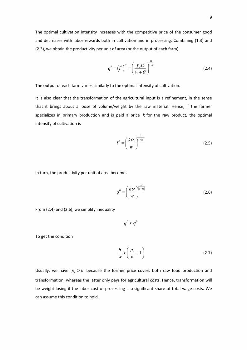
The optimal cultivation intensity increases with the competitive price of the consumer good
and decreases with labor rewards both in cultivation and in processing. Combining (1.3) and
(2.3), we obtain the productivity per unit of area (or the output of each farm):
( )1
* * cp
q lw
α
αα α
θ
− = =
+ (2.4)
The output of each farm varies similarly to the optimal intensity of cultivation.
It is also clear that the transformation of the agricultural input is a refinement, in the sense
that it brings about a loose of volume/weight by the raw material. Hence, if the farmer
specializes in primary production and is paid a price k for the raw product, the optimal
intensity of cultivation is
( )
1
10 k
lw
αα − =
(2.5)
In turn, the productivity per unit of area becomes
( )1
0 kq
w
α
αα − =
(2.6)
From (2.4) and (2.6), we simplify inequality
* 0q q<
To get the condition
1cp
w k
θ > −
(2.7)
Usually, we have c
p k> because the former price covers both raw food production and
transformation, whereas the latter only pays for agricultural costs. Hence, transformation will
be weight-losing if the labor cost of processing is a significant share of total wage costs. We
can assume this condition to hold.

10
A monopolist firm now makes the transformation of the input. This change goes together with
a technological shift in transformation. The unit variable cost of manufacturing, which was
10
θ> in the former production regime switches to zero, while a fixed cost 0F > emerges.
This latter cost was absent before and its arise means that manufacturing ceases to done in
the context of a “cottage” and it becomes performed in a large “factory”.
As it is depicted in Figure 1, the monopolist manufacturing firm has two available locational
strategies.
Consider first the strategy that consists in setting up a single plant in the Foreign country in
order to serve the local market and export back to the Home country. This geographic
concentration strategy allows the firm to save on fixed costs but incurs on higher transport
(trade) costs related with moving the consumer goods across the countries.
The profit function of this concentration strategy is:
( ) ( )1 m mp k Q p k Q Fπ τ= − + − − (2.8)
where
is the fob mill price of the consumer good
is the fob mill price of the agricultural input
is the total output of the consumer good in each country
mp
k
Q
Since we assume that the two goods (agricultural and manufactured) are complementary, the
proportion between their rates of output is fixed. Hence, Q stands for the output of both
goods. Difference in weight between input and output is reflected in the respective prices,
and m
k p .
In profit function (2.8), τ stands for the “iceberg” transport (trade) cost between the two
countries. It is necessary to dispatch exactly 1τ > units of a good from the home country so
that exactly one unit arrives to destination. A share 1τ
τ
− of the sent good is lost in transit.
We also define the following prices,
fob mill price
delivered (full) price
f
d
p
p
≡
≡

11
The relation between and f dp p is given by
amount dispatched from origin
1amount arriving to destination
d
d f
f
pp p
pτ τ= ⋅ ↔ = = > (2.9)
In addition, it is assumed that each seller uses a spatial price policy consisting in charging the
same fob mill price to all its customers.
If the industrial firm decentralizes production by setting up two plants, one in each country,
his profit function is
( )22
mQ p k Fπ = − − (2.10)
Where , and m
k p Q have the same meaning as in (2.8).
The following stage in the game whose extensive form is plotted in Figure 1 entails the
selection of prices by the manufacturer both for the intermediate good, k , and for the
consumer good m
p . We suppose here that the processing firm has two available actions,
namely, either to behave as a monopolist or exiting the market.
If the manufacturer intends to be a monopolist, it is aware that it faces elastic demands, in the
form of a lower bound for the agricultural input and a higher bound for the price of the final
consumer good. Were these bounds not respected, the competitive farmers would have an
incentive to switch to vertical integration of primary production and manufacturing, refining
the input in-house and selling the consumer good directly to the consumers.
Nevertheless, if the manufacturer sets these limiting prices, it may happen that its profit is
negative. Then, the refiner has an incentive to exit the market. A non-coordination situation (a
sort of “poverty trap”) arises, the output of the consumer good being reduced to zero.
Let us consider first that the manufacturer has previously decided to set up a unique plant in
the foreign country, thus concentrating geographically the production. Its profit function is
expressed in (2.8). We have to calculate the prices of the input and the final good, and m
k p
respectively that maximize its profit, while deterring farmers to return to vertical integration.
Clearly, each consumer should be able to purchase the manufactured good at a price m
p not
higher than the competitive price c
p . Hence, m
p fulfills the condition

12
cm
pp
τ≤ (2.11)
It appears as self-evident that the monopolist maximizes profits in (2.8) by quoting output
price as
, where 0, arbitrarily smallcm
pp ε ε
τ= − > (2.12)
Derivation of the limit price for the agricultural product is more involved. Let ( ).R be the land
rent as a function of the price that each farmer receives for his output. Then, intermediate
good price k should lead each farmer to have a rent level at least as high as the level that he
would get by integrating vertically in the context of a competitive market, i.e.
( ) ( )cR p R k≤ (2.13)
( ) ( )* *
c cR p p q w lθ= − + (2.14)
( )cR p is the land rent under vertical integration. * * and q l are the optimal output and input
under vertical integration, being given by (2.4) and (2.3), respectively. It is not difficult to
conclude that the land rent is given by:
( ) ( ) ( )( )
11
11 0
c cR p p
w
α
αα αα
θ
−−
= − > +
(2.15)
Moreover, the land rent of a farmer that only cultivates the land and receives a price k for the
raw agricultural product can be shown to be:
( ) ( ) ( )( )
11
11 0R k k
w
α
αα αα
−−
= − >
(2.16)
Equating (2.15) and (2.16), we have:
( ) ( )cR p R k= (2.17)

13
We solve this equality for price of the input k according to the following steps:
1. Substitute (2.15) and (2.16) into (2.17), and cut the common term ( )1 α− , yielding:
( ) ( ) ( ) ( )
1 11 1
1 1
cp k
w w
α α
α αα αα α
θ
− −− −
= +
2. Take logs and simplifying gives:
ln ln ln 1c
k pw
θα
= − +
3. We assume that the productivity of the transformation task is not much higher than
the reward of the land cultivation task, so that, 1w
θ> but it is small. Then, we can use
the MacLaurin approximation, i.e., ( )ln 1 , for a small x x x+ ≈ , and obtain:
ln ln ck pw
θα≈ −
4. Taking exponentials, simplifying and solving for k , we obtain the input price k that
solves equation (2.17),
c
w
pk
e
θα
≈ (2.18)
Since 1we
θα > , then
ck p< . The manufacturing firm quotes a price k ε+ , 0ε > ,
arbitrarily small, for the intermediate good. This price is lower than the competitive price for
vertically integrated farms.
The output of a farm that only performs agriculture and receives a price slightly higher than
(2.18) for its output is, by analogy with (2.6) , close to
1k
qw
α
αα − =
(2.19)
Substituting (2.18) in (2.19), the farm output becomes

14
( )1
c
w
pq
e w
α
α
θα
α−
=
(2.20)
Since each country has n farms, the output of the consumer good in both the Home and
Foreign countries will be
( )1
c
w
pQ nq n
e w
α
α
θα
α−
= =
(2.21)
Then, we have seen before in (2.8) that the profit function of a monopolist manufacturer that
sets a single plant in the Foreign country is:
( ) ( )1 m mp k Q p k Q Fπ τ= − + − −
Where the first term stands for operating profits in the Home country, the second term
represents profits in the Foreign country (where the single plant is located) and the third term
is minus the fixed cost. This profit function may also be written as:
( )1 2 1m
Q p k Fπ τ= − + − (2.22)
Plugging expressions (2.12), (2.18) and (2.21) into the profit function (2.22), the latter becomes
( )
( )
1
1
21c c c
w w
p p pn F
e w e
α
α
θ θα α
απ τ
τ
−
= − + −
Dividing by 2n , we obtain the profit per inhabitant/farmer:
�
( )
( )
1
11
211
2 2 2
c c c
w w
p p p F
n ne w e
α
α
θ θα α
αππ τ
τ
−
≡ = − + −
(2.23)
Henceforth, we adopt the notation,
� , 1, 22
ii i
n
ππ ≡ = (2.24)

15
Hence, �iπ stands for the per capita profit generated by a monopolist that sets up a number i
(either one or two) of plants.
Consider now the subgame where the manufacturer has previously decide to establish two
plants, so that its profit function is given by (2.10),
( )22
mQ p k Fπ = − −
In this case, and Q k are still given by (2.21) and (2.18), while the fob mill price of the final
good is now equal to c
p since customers live in the neighborhood of a plant. Thus, the
aggregate profit of a manufacturer that achieves proximity to consumers is
( )1
22 2c c
c
w w
p pn p F
e e
α
α
θ θα α
απ
−
= − −
Dividing 2
π by 2n , we obtain the profit per inhabitant as:
�
( )1
22
2
c c
c
w w
p p Fp
n ne e
α
α
θ θα α
αππ
−
≡ = − −
(2.25)
Finding the equilibrium of the game
The class of games depicted in Figure 1 contains purely sequential, perfect information games,
whose subgame perfect equilibrium (SGPE henceforth) can be found very simply by means of
backward induction.
We will reduce this class of games to one defined over three parameters:
• θ ≡ labor productivity in the refinement of the agricultural input when the
processing is made by the farmers themselves, under vertical integration.
• �
2
FF
n≡ ≡ per capita (“per farmer”) fixed cost whenever transformation of the
input occurs under vertical disintegration.
• 1τ > , “iceberg” transport (trade) costs across the two countries.

16
The following specifications of other parameters are made:
1
2α = (3.1)
1c
p = (3.2)
1w = (3.3)
We also give another form to parameter θ , through defining
2we e
θ θα
δ ≡ = (3.4)
It can be seen very easily that δ has the following properties: it is greater than 1, it is strictly
increasing and convex in θ .
δ can be directly interpreted as the “refining rate”, thus given the number of physical units
(e.g., weight units) of the input should be consumed in processing on order to yield one unit of
the final good.
This can be understood easily if we bear in mind the definition of the price of the intermediate
good, k , in (2.18), together with definition (3.2), as we have than
amount of input consumed
amount of consumer good manufactured
wcpe
k
θα
δ = = =
With the numerical specifications (3.1), (3.2), (3.3) and the definition made in (3.4), it is clear
that the profit function of a manufacturer that sets only one plant (written in (2.23) simplifies
to
� �1
1 2 1
4F
τπ
δ τ δ
+ = − −
(3.5)
If the manufacturer opts by settling two plants, then its profit function (written in (2.25))
simplifies to
� �2
1 11 2
2Fπ
δ δ
= − −
(3.6)

17
Since we have a class of games defined in three parameters and two-dimensional plots allow
only to examine game situations in two parameters, we have chosen to assign two different
values for the “iceberg” transport cost τ .
In empirical studies, it is usual to estimate trade costs as a 20% share of total exports or
imports value. Hence, we will assume first that
1 1 5
5 4
ττ
τ
−= ↔ = (3.7)
5
4τ = will be taken as the “normal” or “low” level for transport (trade) costs. By contrast, if
trade relations between the countries deteriorate, the trade cost will be raised to the double
of the level shown in (3.7), i.e.
1 2 5
5 3
ττ
τ
−= ↔ = (3.8)
The case with low transport (trade) costs.
Substituting 5
4τ = in profit function (3.5), condition �1 0π > is regarded to mean the same as
�2
32 45
80F
δ
δ
−< (3.9)
Furthermore, considering profit function (3.6), condition � 2 0π > is equivalent to
�2
1
4F
δ
δ
−< (3.10)
Let us assume now that � �1 2 and π π are both positive. Bearing in mind (3.5) and (3.6), with
5
4τ = , condition � �
2 1π π> can be seen to mean that
�2
8 5
80F
δ
δ
+< (3.11)

18
Figure 2 depicts the regions where inequalities (3.9), (3.10) and (3.11) are satisfied in
parameter space �( ), Fδ for low transport costs 5
4τ
=
.

19
The case with high transport (trade) costs
We now deal with the case with high transport (trade) costs, where 5
3τ = . Substituting this
value of τ in profit function (3.5), the per capita profit of a firm setting up a unique plant is
� �1
2
3 2
10 3Fπ
δ δ= − − (3.12)
The profit of a manufacturer which establishes two plants is still given by (3.6), since no
transport costs are incurred here.
The condition �1 0π > is seen to be equivalent to
�2
9 20
30F
δ
δ
−< (3.13)
Condition � 2 0π > is still equivalent to (3.10). Moreover, condition � �1 2π π< has the same
meaning as
�2
6 5
30F
δ
δ
+< (3.14)

20
Figure 3 shows the regions where inequalities (3.10), (3.13) and (3.14) are satisfied in
parameter space �( ), Fδ for high transport costs 5
3τ
=
.
Transport costs and the degree of industrial transformation as causes
of industrial agglomeration
In this subsection, we assess the impact of transport costs and the degree of input refinement
on the spatial concentration of manufacturing. Taking into account the profit function in (3.5)
concerning the case where a single plant is set up by the industrial firm, we have
� �1
1 2 1
4F
τπ
δ τ δ
+ = − −
(3.15)
The partial first derivative of �1π in relation to the transport cost “iceberg” rate,τ , is negative
�
1
2
1 2 10
4
π
τ δ τ δ
∂ = − + <
∂ (3.16)
This result is natural since decreasing transport costs raises the profit of concentrating
production in a single point in space. If we compute the cross partial derivative in relation to
δ , we obtain
�
1
2 2
1 1 10
π
τ δ δ τ δ
∂ = + >
∂ ∂ (3.17)
Consequently, increasing the refining rate δ dampens the negative effect that increasing
transport costs has upon the profit of a firm, which transacts its input and output across
countries.
We can rationalize (3.17) by recalling that, under the “iceberg” technology, transport costs are
amounts of goods (both manufactured goods and raw materials) that are “lost in transit”
between production and consumption sites. Consequently, increasing the “refining rate”, δ ,
decreases the amount of input that must be carried between the farm and the factory in
21
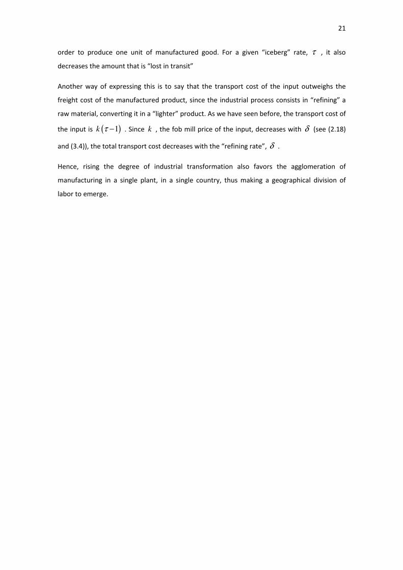
order to produce one unit of manufactured good. For a given “iceberg” rate, τ , it also
decreases the amount that is “lost in transit”
Another way of expressing this is to say that the transport cost of the input outweighs the
freight cost of the manufactured product, since the industrial process consists in “refining” a
raw material, converting it in a “lighter” product. As we have seen before, the transport cost of
the input is ( )1k τ − . Since k , the fob mill price of the input, decreases with δ (see (2.18)
and (3.4)), the total transport cost decreases with the “refining rate”, δ .
Hence, rising the degree of industrial transformation also favors the agglomeration of
manufacturing in a single plant, in a single country, thus making a geographical division of
labor to emerge.

22
Main conclusions
Four main conclusions arise:
a) Division of labor, both occupational and geographical, is caused by low transport costs
(low τ ) and high population density (high n ). Together these two factors bound the
“extent of the market” from above, i.e., they limit the number of workers that are
potentially available to engage in a specialization process6.
b) Geographical division of labor, i. e., concentration of manufacturing in a single plant in
a single country, implies both low transport costs (low τ ) and intermediate population
density (intermediate n ). If density is too small, there will be no vertical
disintegration. By contrast, if the number of inhabitants in each country is too high,
the industrial output will be produced in both countries.
c) The size of “iceberg” transport costs depends on two factors: the rate of the
intermediate good “lost in transit”, 1τ − , and its price k . This price is inversely
related with the “refining rate” δ (see (2.18) and (3.4)), because this is the number of
input units that must be used to produce one unit of consumer good with a fixed
parametric price. If δ is low, then k will be high, so that transport costs will be high
independently of the transport rate τ . Consequently, if the “refinement rate” is low,
manufacturing can start in each country even if transport costs are low.
d) A normative conclusion, stressed by Friedrich List himself, is that geographical division
of labor is socially negative. Indeed “Proximity” yields a higher agricultural output for
each farm and country than “Concentration”. The reason is that “Concentration” is
economical if and only if transport costs are low, as it implies moving inputs and
outputs across countries. “Concentration” is more profitable than “Proximity” as a
location strategy for the monopolist provided that transport costs and the price k of
the raw material are low. The latter condition implies a low intensity of land cultivation
and a small agricultural output in each farm and country. Furthermore, the land rent
expressed in (2.16) decreases with k and becomes lower if the manufacturer installs
only one plant.
6 Amador and Caldeira Cabral (2014) observe that after 2003 Portugal had a sustained surge in exports,
which cannot be easily explained, since the Euro was strong and the oil prices were on the rise. Our
result that a reduction in trade costs conduces to a division of labor between the primary sector and the
industrial sector, can help to explain this occurrence. In fact, in 2003, the EU’s Common Agricultural
Policy (CAP) shifted from product support to producer support, which in practice conduce to a reduction
in the level of protection in the agricultural sector (European Commission, 2012).

23
Discussion
In this paper, we have developed a Listian model of economic development, where the
economy is made up of an primary sector that produces good using a traditional technology
and an industrial sector that can arise if the primary sector specializes in the primary good, i.e.:
if division of labor arises in equilibrium. If division of labor does not occur, the economy is
stuck in an underdevelopment trap. If division of labor does occur, which is limited as in Adam
Smith by the “extent of the market”, industrialization can arise with either industrial dispersion
or agglomeration, i.e., either with or without geographical division of labor.
Geographical labor division is seen to arise if transport costs are low and the “refining rate” in
manufacturing is high. The latter condition implies that the price of the agricultural input is
low, thus diminishing the intensity of its cultivation. In this case, both sectors in the economy –
agriculture and manufacturing – will produce smaller outputs than those that would prevail if
industrial production were decentralized between the two countries.
Otherwise, if the industrial process is not so much “weight-losing”, industrialization can begin
with a decentralized symmetric spatial pattern independently of the transport costs level.
In future work, we wish to look at one of the most innovative ideas by List: economic agents
have incomplete information about trade costs, especially in what concerns trade costs in
international trade. The “randomness” of trade costs can arise because of disruptions in
international trade. These disruptions can be caused for example in extreme cases by wars or
environmental disasters (such as the one in the nuclear plant in Fukushima that putted at risk
the “just in time” system of production of Japanese manufacturers). But the disruptions in
international trade can also be due to more “normal” causes such as different legal systems,
different institutions, or even different culture and language that makes international trade
rules more uncertain.
This line of research is in our opinion very promising, in particular for two reasons. First, to our
knowledge there is very little research on the effects of uncertain trade costs on economic
activity, trade, and location of production. Second, the randomness on trade costs can in our

24
view help to partially explain one of the most important puzzles in international and
macroeconomics: the border puzzle7.
The “border puzzle” refers to the empirical evidence that equally distant regions, trade much
more with each other, even after correcting for trade barriers, if they are located in the same
country than if they are located in different countries. For instance, McCallum (1995) finds that
in 1988, trade between Canadian provinces was 2,200 percent larger than the trade between
U.S. states and Canadian provinces.
In this way, a border between two countries might just introduce an uncertainty that reduces
international trade across borders. In future work, we will try to verify this assertion.
7 Obstfeld and Rogoff (2001) defend that the border puzzle is one of the six puzzles of open economy
macroeconomics.
25
References
Amador, J. and Caldeira Cabral, M. (2014), A Economia Portuguesa no Contexto Global, in
Alexandre, F. (ed.), A Economia Portuguesa na União Europeia - 1986-2010, Coimbra,
Conjuntura Actual Editora.
Becker, G. and Murphy, K. (1992), The Division of Labor, Coordination Costs, and Knowledge,
Quarterly Journal of Economics, 107, 1137-1160.
European Commission (2012), The Common Agricultural Policy: A Story to be Continued,
Luxembourg: Publications Office of the European Union.
Francois, P. and van Ypersele, T. (2002), On the Protection of Cultural Goods, Journal of
International Economics, 56, 359–369.
Glaeser, E. and Gottlieb, J. (2009), The Wealth of Cities: Agglomeration Economies and Spatial
Equilibrium in the United States, Journal of Economic Literature, 47, 983–1028.
Glaeser; E. (1989), Are Cities Dying?, Journal of Economic Perspectives, 12, pp. 139-160
Harlen, C. (1999), A Reappraisal of Classical Economic Nationalism and Economic Liberalism,
International Studies Quarterly, 43, 733–744.
Krugman, P. (1984), Import Protection as Export Promotion: International competition in the
Presence of Oligopoly and Economies of Scale, in Kierzkowski, H. (ed.), Monopolistic
Competition in International Trade, Oxford, Clarendon Press.
Krugman, P. (1991), Increasing Returns and Economic Geography, Journal of Political Economy,
99, 413-499.
Krugman, P. (1993), The Hub Effect: or, Threeness in Interregional Trade, in Ethier, W.;
Helpman, E. and Neary, P. (eds.), Theory, Policy and Dynamics in International Trade: Essays in
honor of Ronald W. Jones, Cambridge: Cambridge University Press.
Levi-Faur, D. (1997a), Friedrich List and the Political Economy of the Nation-State, Review of
International Political Economy, 4, 154–178.
Levi-Faur, D. (1997b), Economic Nationalism: From Friedrich List to Robert Reich, Review of
International Studies, 23, 359–370.

26
List, F. (1841), The National System of Political Economy, London, Frank Cass.
McCallum, J. (1995), National Borders Matter: Canada-U.S. Regional Trade Patterns, American
Economic Review, 85, pp. 615-623.
Obstfeld; M. and Rogoff, K. (2001), The Six Major Puzzles in International Macroeconomics: Is
There a Common Cause? In Bernanke, B. and Rogoff, K. (eds.), NBER Macroeconomics Annual
2000, Volume 15.
Pais, J. and Pontes, J. (2008), Fragmentation and Clustering in Vertically-Linked Industries,
Journal of Regional Science, 48, 991-1006.
Pontes, J. (1992), Division of Labor and Agglomeration Economies, Estudos de Economia, 12,
123-132.
Sai-wing Ho, P. (2005), Distortions in the Trade Policy for Development Debate: A Re-
Examination of Friedrich List, Cambridge Journal of Economics, 29, 729-745.
Scott, A. (1983), Industrial Organization and the Logic of Intra-Metropolitan Location: I.
Theoretical Considerations, Economic Geography, 59, 233-250.
Scott, A. (1986), Industrial Organization and Location: Division of Labor, the Firm, and Spatial
Process, Economic Geography, 62, 215-231.
Smith, A. (1776), An Inquiry into the Nature and Causes of the Wealth of Nations, Oxford, OUP.
Stigler, G. (1951), The Division of Labor is Limited by the Extent of the Market, Journal of
Political Economy, 59, 185-193.
Williamson, O. (1981), The Modern Corporation: Origins, Evolution, Attributes, Journal of
Economic Literature, 19, 1537-1568.
Young, A. (1928) Increasing Returns and Economic Progress, Economic Journal, 38, 527-42.

27