Applied Energy 106 (2013) 100–115

Contents lists available at SciVerse ScienceDirect

Applied Energy

journal homepage: www.elsevier .com/ locate/apenergy

Economic appraisal of shale gas plays in Continental Europe

0306-2619/$ - see front matter � 2013 Published by Elsevier Ltd.http://dx.doi.org/10.1016/j.apenergy.2013.01.025

⇑ Address: Department of Geoscience & Engineering, Delft University of Tech-nology, Stevinweg 1, Delft 2628CN, Netherlands.

E-mail address: R.Weijermars@TUDelft.nl

Ruud Weijermars ⇑Department of Geoscience & Engineering, Delft University of Technology, Stevinweg 1, Delft 2628CN, NetherlandsAlboran Energy Strategy Consultants, Delft, Netherlands

h i g h l i g h t s

" Economic feasibility of five European shale gas plays is assessed." Polish and Austrian shale plays appear profitable for P90 assessment criterion." Posidonia (Germany), Alum (Sweden) and a Turkish shale play below the hurdle rate." A 10% improvement of the IRR by sweet spot targeting makes all plays profitable.

a r t i c l e i n f o

Article history:Received 21 May 2012Received in revised form 13 December 2012Accepted 7 January 2013

Keywords:Shale gasWell productivityCash flow analysis

a b s t r a c t

This study evaluates the economic feasibility of five emergent shale gas plays on the European Continent.Each play is assessed using a uniform field development plan with 100 wells drilled at a rate of 10 wells/year in the first decade. The gas production from the realized wells is monitored over a 25 year life cycle.Discounted cash flow models are used to establish for each shale field the estimated ultimate recovery(EUR) that must be realized, using current technology cost, to achieve a profit. Our analyses of internalrates of return (IRR) and net present values (NPVs) indicate that the Polish and Austrian shale playsare the more robust, and appear profitable when the strict P90 assessment criterion is applied. In con-trast, the Posidonia (Germany), Alum (Sweden) and a Turkish shale play assessed all have negative dis-counted cumulative cash flows for P90 wells, which puts these plays below the hurdle rate. The IRR forP90 wells is about 5% for all three plays, which suggests that a 10% improvement of the IRR by sweet spottargeting may lift these shale plays above the hurdle rate. Well productivity estimates will become betterconstrained over time as geological uncertainty is reduced and as technology improves during the pro-gressive development of the shale gas fields.

� 2013 Published by Elsevier Ltd.

1. Introduction

There is a growing interest in the assessment of the world’sshale gas resource potential, which has intensified regional explo-ration efforts that must establish the presence and volume of pro-spective natural gas resources. US shale gas fields provideimportant guidance for the economic development of shale gaswells in emergent shale plays elsewhere in the world. A principalreason why the development of shale plays remains economicallyrisky is that the estimated ultimate recovery (EUR) is poorly con-strained during the early stages of field development.

We model the economic potential of five potential Europeanshale gas fields. Not all shale gas plays are equal, and reservoirquality varies within the plays and between the plays as hasbecome apparent from US shale plays. Fig. 1a provides a concise

overview of the major US shale gas growth areas [1]. By 2009,the production of US domestic gas from unconventional resources(tight sands, coal beds and shale) surpassed the domestic output ofconventional gas [2]. By 2012, shale gas accounted for over half ofall the US gas produced from unconventional (or continuous) re-sources. Fig. 1b shows that the marginal breakeven costs for USshale gas basins differ [3], which is a consequence of variationsin well productivity (due to intrinsic petro-physics of the reservoirand the variation in well effectiveness) and differences in fielddevelopment cost.

This study makes a first attempt to evaluate the economics offive potential shale gas plays in Europe (Austria, Germany, Poland,Sweden and Turkey). Well productivity type curves are establishedfor each play based on an earlier review of estimated ultimaterecovery (EUR) for the plays [4]. Decline curve analysis providesthe well productivity model that fits the prior published EUR data.Subsequently, the net present value (NPV) and internal rate of re-turn (IRR) of each shale play are calculated by applying discountedcash flow analysis, using representative inputs for gas price, pro-

Fig. 1. (a) Major US shale gas plays and production since 2000 [1]. (b) Breakeven marginal prices for major US shale gas play, duly accounted for or limited to ‘‘best’’ wellperformance. (Data source: Bloomberg & Credit Suisse [3]).

R. Weijermars / Applied Energy 106 (2013) 100–115 101

duction cost, taxes, depreciation and discount rate. The sensitivityof IRR and NPV to variations in EUR is modeled for each play, whichthus provides the minimum EUR for which wells are economic – adirective for ‘sweet spot targets’. A stochastic approach that ac-counts for the spatial spread of well productivities is included,using production volume probabilities P10–P50–P90. The spreadin NPV and IRR related to the well productivity uncertainty rangeprovides an indication for the risk taken when only few wells aredrilled and provides a screening criterion for selecting the bestfield development opportunities.

2. European shale plays

Europe’s unconventional gas resources in place were firstranked in a global perspective by Rogner [5], who estimated some1255 trillion cubic feet (Tcf) gas in place from the following uncon-ventional resources: shale gas: 549 Tcf; tight sands: 431 Tcf; and

Fig. 2. (a) Relative sizes of Europe’s largest conventional gas fields (Groningen, Trollrecoverable unconventional gas. (b) World shale gas inventory of 2011 estimates 425 Tcspread of the 18 Tcm is indicated by the horizontal bars (Source: DOE/EIA [8]; Weijerma

coal-bed methane: 275 Tcf. Europe ranks at the lower end of globalunconventional resource potential, with only 4% of the worldwidetotal (Asia and North America lead, with respectively 30% and 25%of GIP). This is partly due to the exclusion of Poland, Hungary andRomania in Rogner’s assessment of 1997 [5]; appraisals for thesecountries were not available at that time.

The technically recoverable shale gas volumes for Europe wereestimated to range between 150 and 200 Tcf by WoodMacKenzie[6]. CERA [7] considered technically recoverable shale gas to rangebetween 106 to 423 Tcf (3–12 Tcm), and the US Department of En-ergy raised this to 18 Tcm [8]. This number also has been con-firmed in resource appraisals by BGR [9], Medlock et al. [10] andin the review by McGlade et al. [11]. Fig. 2a places the shale gas re-source estimates in perspective by comparison to Europe’s threemajor producing conventional gas fields (Groningen in Nether-lands; Troll and Ormen Lange on Norway’s Continental Shelf).Fig. 2b confirms that the TRR estimates differ greatly per country:

and Ormen Lange Gas Fields), and an early estimate of 12 Tcm for Europe’s totalm recoverable resources, of which only 18 Tcm (4%) occurs in Europe. The countryrs and McCredie [12]).

Table 1Selected properties European shale gas basins. Data Source: Kuhn and Umbach [4].

Property Alum Sweden Silurian Poland Posidonia Germany Shale Austria Shale Turkey

Basin area (Sq. km) 2010 23,816 7500 900 18,000Depth (m) 100–3500 2000–4000 0–2500 4500–8000 2500–3500Thickness (m) 30–100 30–300 20–500 1,500 100–400TOC (%) 2–25 7 2–12 1.5–2 4Ro (%) 1.4–3.0 1.0–4.0 0.5–1.5 0.7–1.6 0.5–3.0Tcf (OGIP) 39 844 94 750 151RF 0.14 0.17 0.18 0.04 0.15EUR/Wella (Bcf) 40 years 4.8 4.8 4.8 8 2.2

a Used as input for Table 2.

Fig. 3. (a) Production profiles for single gas wells with initial production rates qi = 0.3, 0.5 and 1 bcf/year and a decline factor of 15% (a = �0.15). (b) Cumulative production(25 year lifecycle) gives corresponding EUR of 1.97, 3.25 and 6.55 bcf/well.

Fig. 4. (a) Production profiles for gas field projects with 100 wells, drilled over a decade at a rate of 10/year, each well with qi = 0.3, 0.6 and 1 bcf/year and a = �0.15. (b)Cumulative production (25 year lifecycle) gives the corresponding EUR of 192, 320 and 640 bcf for the respective fields.

102 R. Weijermars / Applied Energy 106 (2013) 100–115

Poland, France, Norway and Ukraine host the larger estimates. Thepie diagram included in Fig. 2b gives a summary of the TRR esti-mates for shale around the world, as estimated by AdvancedResource International in a study commissioned by the US Depart-ment of Energy [8]. This inventory confirms that Europe’s 18 Tcmof shale gas potential is a relatively poor endowment comparedto other world regions. However, if fully developed, these

resources could provide Europe with another 25 years of naturalgas supplies at projected consumption levels of between 600 and700 bcm/year. The strategic vulnerability of natural gas supply toEurope due to its growing reliance on imports has been highlightedelsewhere [12–14].

Poland is Europe’s leading shale gas resource holder (Fig. 2b). Italso has the largest proportion of coal (55%) in its primary energy

Fig. 5. Continental European gas price trend mode, forward corrected for inflation,using Eq. (2) and Pi = $10/Mcf and b = 0.025.

Table 2Selected rates European shale gas basins.

AlumSweden

SilurianPoland

PosidoniaGermany

ShaleAustria

ShaleTurkey

EUR/Well (Bcf-25 years)a

3.25 3.25 3.25 6.55 1.97

Productivity year 1flow rate (bcf/year)a

0.50 0.50 0.50 1.00 0.30

Well CAPEX ($/MM)b 15 14 13 24.5 8.1OPEX ($/Mcf)b 0.6 0.5 0.6 0.4 1.2Other OPEX ($/Mcf)b 1.4 1.0 1.2 1.0 1.0Royalty rate (%)b 0 1.5 8 10 13Corporate tax (%)b 28 19 30 25 20Depreciation (%)c 10 10 10 10 10Discount rate (%)c 5 5 5 5 5

a Data Source: Prorated from Table 1.b Data Source: Kuhn and Umbach [4].c Data Source: Alboran Research.

R. Weijermars / Applied Energy 106 (2013) 100–115 103

supply. The production of natural gas from its indigenous shale re-sources could help Poland reduce greenhouse gas emissions byreplacing coal as the fuel of choice for its aging coal-fired powerstations, as well as reduce Poland’s dependency on Russian gasimports.

France possesses Europe’s next largest shale gas resource base(Fig. 2b), but the local opposition against shale gas developmentis significant and it is set to maintain its nuclear options. Opposi-tion to shale gas development finds stronger political support incountries where shale gas threatens to displace existing energysources with a strong support base (like the nuclear power lobbyin France).

Norway has substantial shale gas resources (Fig. 2b), but devel-opment may be slow. Shale gas will have to compete with the moreprofitable conventional gas production from the Norwegian conti-nental shelf. Even without actualizing its shale gas potential, Nor-way remains Europe’s major oil and gas producer and exporter fordecades to come.

Ukraine holds Europe’s fourth largest shale gas deposits(Fig. 2b), but has an energy policy that is still influenced by Russianenergy strategy. As a result, development of shale gas in Ukrainewill be politically much more complex than in Poland.

Sweden is Europe’s smallest gas consumer, with gas accountingfor only 2.6% of its primary energy supply and no gas retail market.The development of shale gas would require the development of alocal gas market with the additional infrastructure constraints. TheAlum shale potential for commercial gas production has been neg-atively assessed by Shell engineers [15].

Denmark, the UK, the Netherlands and Germany are all majorgas consumers, with extensive gas infrastructure and mature retailmarkets. Their domestic gas supply from conventional sources isdeclining. These countries are well placed to benefit from domesticshale gas development, which could delay expensive gas imports.The strategic importance of shale gas development for the Nether-lands has been outlined elsewhere [16,17].

The outlook for shale gas in Europe has been briefly evaluated inearlier studies [4,18–21]. Table 1 provides a concise overview ofkey data for five emerging shale plays. Europe’s gas shales areunderexplored, and any estimates about possible well economicsare very preliminary. The Posidonia shale has been alluded to asa close analog of the Woodford shale [19], which enables a reser-voir analog approach [22] for an early assessment of its resourcepotential.

3. Methodology

The results documented in this study are based on genericequations for discounted cash flow analysis (DCF analysis, Appen-dix A) and well productivity decline analysis (DCA methodology,Appendix B). The algorithms are incorporated in a proprietary ex-cel-based interface developed by Alboran Energy Strategy Consul-tants, which enabled the calculation of field development scenariosand was used to produce the plots in the present study. A concisemanual is made available as a complimentary resource in an onlinerepository [23]. The supporting methodologies are outlined inAppendices A–D.

3.1. Well productivity model

Understanding the well productivity of representative US shalegas plays provides important guidance for the economic develop-ment of shale gas wells in emergent shale plays elsewhere in theworld. A review of US well productivities, using 46,506 shale gaswells, gives a 40-year mean EUR of 1.14 Bcf [24]. In the Barnett,the mean EUR for representative horizontal wells is 1.4 bcf/well[25], but there is considerable spread in well performance for suba-reas. In the ‘best areas’ for the Barnett a representative mean EUR is2.1 bcf/well, and the ‘worst areas’ have a mean EUR of 0.59 bcf/well[25].

For this study, we assume the well EUR can be modeled by anexponential decline function:

qn ¼ qið1þ aÞn ð1Þ

qn is the flow rate in year n, qi the starting flow rate in first year, and‘a’ the annual decline rate (remember this is a negative fraction),and ‘n’ the number of years.

Fig. 3a plots the well productivity over a 25 year lifecycle(n = 1,. . .,25) using the gas production type curves for single wellsin each of the five shale plays assessed here. Estimates for the25 year lifecycle EUR/well (Table 2) are prorated from the EUR/wellfor a 40 year lifecycle (Table 1, based on review by Kuhn and Um-bach [4]). The well flow rates of Fig. 3a were obtained by fitting theEUR with an appropriate decline function using Eq. (1). The corre-sponding cumulative production over the 25 year well life is givenin Fig. 3b.

Fig. 4a shows the annual production for the individual fielddevelopment projects in the shale plays drilling 100 wells in the

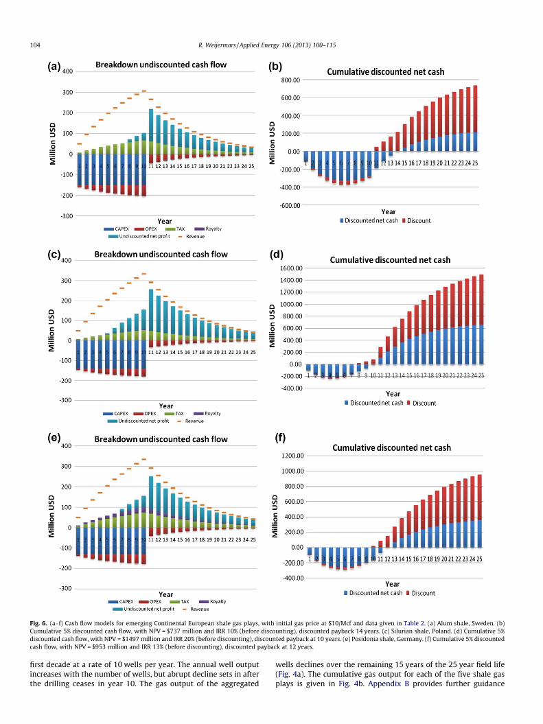
Fig. 6. (a–f) Cash flow models for emerging Continental European shale gas plays, with initial gas price at $10/Mcf and data given in Table 2. (a) Alum shale, Sweden. (b)Cumulative 5% discounted cash flow, with NPV = $737 million and IRR 10% (before discounting), discounted payback 14 years. (c) Silurian shale, Poland. (d) Cumulative 5%discounted cash flow, with NPV = $1497 million and IRR 20% (before discounting), discounted payback at 10 years. (e) Posidonia shale, Germany. (f) Cumulative 5% discountedcash flow, with NPV = $953 million and IRR 13% (before discounting), discounted payback at 12 years.

104 R. Weijermars / Applied Energy 106 (2013) 100–115

first decade at a rate of 10 wells per year. The annual well outputincreases with the number of wells, but abrupt decline sets in afterthe drilling ceases in year 10. The gas output of the aggregated

wells declines over the remaining 15 years of the 25 year field life(Fig. 4a). The cumulative gas output for each of the five shale gasplays is given in Fig. 4b. Appendix B provides further guidance

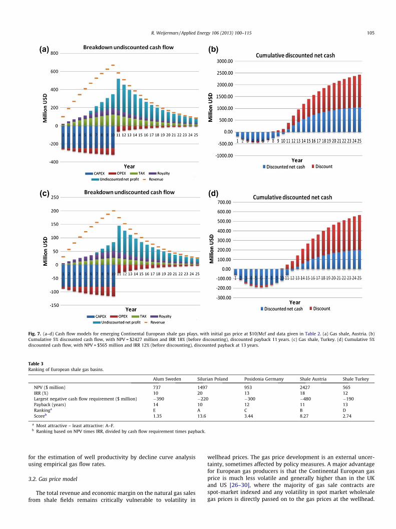
Fig. 7. (a–d) Cash flow models for emerging Continental European shale gas plays, with initial gas price at $10/Mcf and data given in Table 2. (a) Gas shale, Austria. (b)Cumulative 5% discounted cash flow, with NPV = $2427 million and IRR 18% (before discounting), discounted payback 11 years. (c) Gas shale, Turkey. (d) Cumulative 5%discounted cash flow, with NPV = $565 million and IRR 12% (before discounting), discounted payback at 13 years.

Table 3Ranking of European shale gas basins.

Alum Sweden Silurian Poland Posidonia Germany Shale Austria Shale Turkey

NPV ($ million) 737 1497 953 2427 565IRR (%) 10 20 13 18 12Largest negative cash flow requirement ($ million) �390 �220 �300 �480 �190Payback (years) 14 10 12 11 13Rankinga E A C B DScoreb 1.35 13.6 3.44 8.27 2.74

a Most attractive – least attractive: A–F.b Ranking based on NPV times IRR, divided by cash flow requirement times payback.

R. Weijermars / Applied Energy 106 (2013) 100–115 105

for the estimation of well productivity by decline curve analysisusing empirical gas flow rates.

3.2. Gas price model

The total revenue and economic margin on the natural gas salesfrom shale fields remains critically vulnerable to volatility in

wellhead prices. The gas price development is an external uncer-tainty, sometimes affected by policy measures. A major advantagefor European gas producers is that the Continental European gasprice is much less volatile and generally higher than in the UKand US [26–30], where the majority of gas sale contracts arespot-market indexed and any volatility in spot market wholesalegas prices is directly passed on to the gas prices at the wellhead.

Fig. 8. (a) Sensitivity of IRR per well to EUR variations. (b) Sensitivity of discounted NPV per well to EUR variations for each of the five plays analyzed here. Dots show the EURvalues corresponding to the estimates given in Table 2.

106 R. Weijermars / Applied Energy 106 (2013) 100–115

Continental wholesale gas prices have been between two to fivetimes higher than in the US (between 2008 and 2012), becauseContinental European gas contracts are still predominantly oil-in-dexed and long-term [29]. UK gas prices tend to move in a pricedeck between US and Continental European gas prices [30]. US spotgas prices have collapsed due to overproduction of natural gas inthe closed North American market. The North American spot gasprices continue to depress the wellhead prices of all gas producerswho deliver their gas on spot-market indexed contracts.

Our cash flow models for shale gas plays in Continental Europeadopt an initial gas price set at $10/Mcf, with a forward correctionfor inflation modeled by an annual inflation factor of 2.5% (Fig. 5):

pn ¼ pið1þ bÞn ð2Þ

pn is the wellhead gas price in year n, pi the wellhead gas price inthe first year, and ‘b’ the annual inflation rate affecting the gas price,and ‘n’ the number of gas production years. In our models 1000 cu-bic ft (1 Mcf) of gas is equivalent to a calorific value of 1 million Brit-ish thermal units (1 Mbtu) used in market pricing. Alternativefunctions for modeling gas price trends and background on whatdrives regional gas prices are highlighted in Appendix C.

3.3. CAPEX, OPEX and taxes

The outlay of capital expenditure (CAPEX) and operating expen-diture (OPEX) can be controlled by the operator. Appendix D sum-marizes the basics of CAPEX estimates and factors affectingcorporate cost of capital (both controllable), discusses the detailsof OPEX outlays (controllable), and provides examples of royalties,tax rates, depreciation, and discount rates – all of which affect theoutcome of the cash flow model for a specific field asset. The taxesand royalties due are mostly controlled by the governing petro-leum extraction laws and rules. Table 2 shows the typical valuesused in our cash flow model simulation for the European shalegas fields.

4. DCF analysis of European shale plays – base case

Our discounted cash flow (DCF) models for the shale plays inContinental Europe are based on the production profiles of Fig. 4aand b, a common gas wellhead price assumption of Fig. 5, and thespecific field development expenditures as specified in Table 2.

The cash flow models, based on the base case well rates of Fig. 4aand b, show positive internal rates of return for all five major Euro-pean prospective shale gas plays (Figs. 6 and 7). The IRR ranges be-tween 20% for Polish Silurian shale at the top-end and 10% forSwedish Alum shale at the bottom-end. The undiscounted cash flowdiffers for each shale gas project (Figs. 6 and 7, left-hand panels) dueto the differences in estimated well performance (EUR, Table 1), dif-ferent cost base (OPEX, CAPEX) and more or less favorable royaltyand taxation rates (Table 2). For all fields, the plateau of cumulativediscounted cash flow is reached 25 years after the start of thestandardized 100 well field development program (Figs. 6 and 7,right-hand panels). For the same 25 year lifecycle, the NPVs are alldifferent, controlled by the local well productivity, cost structureand taxation policy. The 100 well field development project representsdifferent NPV in different plays: $737 million in the Alum shale(Sweden), $1497 million in the Silurian shale (Poland), $953 millionin the Posidonia shale (Germany), $2427 million in the Austrianshale, and $565 million in the Turkish shale. The annualized reve-nues and break-down of the costs and benefits are specified in theundiscounted cash-flow curves of Figs. 6a,c, and e and 7a and c.

The outcome of the base case cash flow models for Europeanshale plays (Figs. 6 and 7) are ranked, according to the key perfor-mance indicators (KPIs) given in Table 3. The ranking is based onNPV times IRR, divided by cash flow requirement times Payback.Our ranking suggests that Polish shale provides the most attractiveinvestment option and Alum shale the least attractive.

4.1. Sensitivity of IRR and NPV to well productivity variations

Considerable uncertainty in our assessment of European shalegas economic resides in the EUR/well assumed for each play(Table 2). No conclusive well performance data are available fromany European well tests. Well productivities for European shaleplays can be constrained using US well analogs, which is practicaluntil the first European development projects will finally getstarted. Based on comparisons to US analogs we can alreadyconclude that the published EURs [4] seem optimistically highcompared to productivities of US shale gas analog basins; theEUR is probably between 1.5 and 3 times too optimistic (authorview). Given that the Woodford (�2 bcf/well, 25 year) provides aclose analog for the European Posidonia shale, its estimated EURof 3.25 bcf/well (25 year) may be 1.6 times too optimistic.

Fig. 9. (a and b) Uncertainty range of well productivity used P10–P50–P90 gas flow rates as input for cash flow projections for each of the five plays considered. (a) Spread inannual undiscounted net cash flow (in million USD) due to uncertainty about well productivity that can be realized (P10 – upper green curve for best wells; P50 – middle redcurve for average wells, and P90 – lower blue curve for below average wells). (b) Corresponding spread in cumulative discounted net cash (equal to the discounted NPV) inmillion USD. (For interpretation of the references to color in this figure legend, the reader is referred to the web version of this article.)

R. Weijermars / Applied Energy 106 (2013) 100–115 107

We performed a Monte-Carlo simulation to calculate the sensi-tivity of the IRR and NPV on well productivity for the five playsconsidered. Fig. 8a summarizes the IRR sensitivity to spatial varia-tions in well productivity (which determines the EUR). The Turkish

shale play considered here is best positioned for a rapid improve-ment of the IRR when well productivities improve during the pro-gressive development of the shale gas field as geologicaluncertainty is reduced and technology improves. Of all shale

108 R. Weijermars / Applied Energy 106 (2013) 100–115

projects assessed here, the IRR of the Austrian shale play is leastsensitive to EUR fluctuations (Fig. 8a). Additionally, the sensitivityof the discounted NPV to EUR variations for each field developmentproject is summarized in Fig. 8b. The NPV is highest for the Aus-trian shale based on the well EUR estimations of Table 2. TheNPV sensitivity to EUR variations is nearly similar for all plays con-sidered. Differences in tax and royalty rates between the variouscountries are responsible for the slopes of NPV lines not beingstrictly parallel.

The results of Fig. 8a and b show the sensitivity of IRR and NPVto variations in individual well productivities within shale fields.The EUR range shown in Fig. 8a and b can be assumed representa-tive for P50 wells in the shale plays considered. However, in theearly development stage of an emergent shale gas play, it is unli-kely that P50 well productivity can be attained when only a fewwells are drilled. In order to provide an indication of the risk takenwhen only few wells are drilled, we incorporated into the dis-counted cash flow model a stochastic well productivity range,using a P10–P50–P90 spread for the gas flow rate (P90 for 90% cer-tainty; P50 for 50% certainty and P10 for 10% certainty). The P50values adopted in Table 2 for each play were assigned a Gaussiandistribution for the well productivity spread with best wells(P10) set at 4/3 times P50 values (and P90 wells at about 3/4 timesP50 values). These seem reasonable well productivity ranges basedon our analysis of well spreads in US shale gas fields.

The undiscounted annual net cash flow and the correspondingcumulative discounted cash flow for P10–P50–P90 wells are sum-marized in Fig. 9a and b. These results provide additional criteriafor play ranking. New shale plays in Europe and elsewhere haveno producing shale gas wells to constrain the uncertainty of wellproductivity. Using P50 for a first economic appraisal cannot be jus-tified as the likelihood of evening out poor P90 wells with excellentP10 wells (sweet spots) is not present in emerging shale gas playswhere the value of information is limited in the early stage of fielddevelopment. Companies should use in their economic appraisalthe SPE Petroleum Resource Management System [31] and theSEC reserve reporting guidelines [32], which require conservative90% certainty for EUR estimates of proved reserves. Contingent re-sources can be upgraded to reserves only when commercially pro-ducible. Companies therefore are well advised to use the EURvolume of P90 wells to assess the NPV of a new shale gas field.Fig. 9b shows that the P90 discounted cumulative net cash is zerofor the Alum shale (Sweden), the Posidonia shale (Germany) andTurkey shale. This means their discounted P90 NPVs are all zero.In contrast, the discounted P90 NPVs for the Silurian shale in Polandand the Austrian shale are both positive, turning these two playsinto the most attractive field development projects of the five op-tions assessed. However, the IRR for P90 wells in the Posidonia (Ger-many), Alum (Sweden) and Turkish shale plays is about 5% for allthree plays assessed (5%, 5% and 4.7%, respectively), which meansthat a 10% improvement in the IRR due to sweet spot targetingmay lift the latter three shale plays above the corporate hurdle rate(commonly set at 15%).

5. Discussion and conclusions

For the sustained success of shale gas operations in North Amer-ica, and for the successful development of new shale gas plays else-where in the world, the returns on investments in shale gasprojects must remain profitable. A recent study by the US NationalPetroleum Council [33] stated that cheap and abundant US shalegas supplies could be sustained for long periods of time. Brooks[34] pointed out the weak economic fundamentals and inadequateeconomic assessment. The NPC report [33] ignored supply and de-mand dynamics currently setting wellhead prices for natural gas at

levels well below the true economic cost required to develop shalegas resources. Persistently low US natural gas prices have put se-vere pressure on the operational earnings of US natural gas produc-ers since mid 2008. North America’s shale gas companies havebeen unable to demonstrate a competitive advantage over conven-tional operators [35], weakened by gas prices that remain low aslong as gas output rises faster than demand in a closed NorthAmerican gas market.

Cash flow analysis of a representative peer group of US shale gasoperators [35,36] showed that their 2009 income was negative,whereas the income of the integrated oil majors remained robust.Clearly, North American shale gas plays are not the easy cash cowsas sometimes asserted, and operational profits are presently notmaterializing for a large number of US and Canadian shale gas oper-ators [37]. Land acquisition cost is increasingly booked by shale gascompanies as sunk cost, separate from operational results, and be-comes part of a land speculation investment. Consequently, onlypart of the current depletion, depreciation, and amortization isaccounted for in the commercial assessment of Fig. 1b.

Field development plans for shale gas assets must use invest-ment models based on realistic estimates of well productivity,price volatility and field development costs to ensure cash flow willremain positive [38]. This study is a first attempt to provide suchmodels for emerging shale gas plays in Continental Europe. Thecash flow models outlined in this study are based on well produc-tivity decline curve analyses, which show cumulative cash flowswill reach plateau after between 10 and 20 years of production.Longer well-lifecycle assumptions seem unrealistic for the eco-nomic assessment of shale gas plays in Europe and elsewhere.Emerging shale gas plays typically have a high degree of subsurfaceuncertainty due to which field development in the early stage inev-itably includes wells with a lower productivity and marginal cashflow. The mean EUR for the field can grow when drilling rigs zoomin on the so-called sweet spots of a developing shale gas play. Weshowed a play ranking methodology based on the product of NPVand IRR divided by cash flow times payback to rank the relative va-lue potential and economic viability of European shale gas prov-inces. This revealed the Polish Silurian shale as the mostpromising target and the Swedish Alum shale as the least promis-ing target. The rankings of the other major European shale gasprospects are included in Table 3.

A bottleneck for the development of shale gas resources in Eur-ope and elsewhere could become the stakeholder discussion,which delays the approval speed for the required permits. Min-eral-rights are administered and granted by the federal govern-ment in all European nations – and not by the landowners like inthe US. A major hurdle for commercial development of Europeanshale gas plays lies in the slow and complex decision-making pro-cess for exploration and production licenses.

Local municipality councils can uphold the permission to drill.For example, Cuadrilla Resources planned to drill and test justtwo wells in the Netherlands in 2011, but local authorities underpressure of local community activists delayed the drilling plansfor over a year (an a quick resolution seems remote). The modestfield development rate of 10 well per year assumed in our analysisis slow compared to US standards, where several hundred wellshave been annually drilled in active shale gas plays.

In each country, time to first production can be accelerated ifthe IEA golden rules [39] are applied to provide incentives for shalegas operators so these can establish an operational scale requiredto support a cost-effective shale gas service industry. Most produc-tion acreage in Western Europe is already under production li-censes by conventional oil and gas companies, which handicapsthe development of the unconventional resources. As long as con-ventional oil and gas fields remain profitable to the current conces-sion holders, they are unlikely to farm-out their lucrative acreage

Fig. A1. (a) Annual cash flow (A in Eq. (A1)) over the 25 year lifecycle of a synthetic gas project. (b) Cumulative cash flow or net present value for this project climbs to 800million USD if undiscounted for the time value of money [taking discount factor F = 0 in Eq. (A3), giving maximum possible NPV@0%]; for a discount rate of 25% this projecthas NPV = 0, which is why the IRR for this project is 25%.

R. Weijermars / Applied Energy 106 (2013) 100–115 109

for shale gas extraction for fear of negative press from shale gascritics. In Eastern Europe, the situation is different: plenty of shaleacreage has been acquired by major oil companies and smallerindependents alike, with the specific purpose to explore and devel-op shale gas and tight gas resources.

Once exploration licenses are granted, shale gas companies canset out to explore and begin to evaluate TRR, IRR and NPV esti-mates which are essential to assess the profit potential of thenew shale gas plays. Shale gas operators must zoom in on leads,prospective resources and then proceed to detect sweet spots thatprovide the attractive EUR for proved reserves. Rigorous economicanalysis of shale gas wells under various assumptions is requiredto assure the sustainability of shale gas production and future fielddevelopment activity [40]. Operationally Europe still has a lack ofland gas rigs and mobile fracking fleets, all of which have to bebrought in from US suppliers. This will make their deploymentpotentially more costly than in the US. Well performance metricsand cost control as well as tax liabilities also affect the EUR growthrate. Proved reserves can be claimed as collateral for further inves-tor support, but securing the first reserves may require tens ofwells to be drilled which is often beyond the means of junior shalegas companies.

To bring the new shale gas to market there must be a referencewellhead price from a regional gas market that includes the cost ofgathering and connection to the main grid. If not yet established,such tie-in cost must be socialized and preferably co-financed bya gas transmission company with support from the national gasgrid owners. If the cost of new gas gathering systems is prohibitive,gas-to-wire solutions may provide an attractive alternative.

Earlier studies have shown that drilling about 1000 wells peryear would after 5 years result in 1 Tcf (�28.5 bcm) gas productionfor Europe [18,19]. A production output of 1 Tcf/year would coverapproximately 5% of Europe’s gas demand, but its realization is un-likely to proceed fast. Unless new policies clear the way to facilitatefaster drilling permission processes, operators cannot turn shalegas plays into profitable business opportunities. Our appraisalemphasizes that discounted cash flow models are paramount forsetting effective targets for production output and well technologyexpenditure to ensure positive returns on investment in new shalegas plays. The commercial success of shale gas operators in Europe

and elsewhere will be determined by their ability to control fielddevelopment cost and optimize cash flow by selective drilling ofonly the most attractive resource opportunities.

We developed our own cash flow model, which is used byAlboran Energy Strategy Consultants for proprietary studies andfield development plan evaluation. Numerous other software pack-ages for financial modeling and evaluation of oil and gas projects areavailable from the market. While these model tools can be helpful,they do not provide a guarantee that output is relevant if users areindifferent to the complexities of assessing shale gas economics.Concepts like stochastic or discrete uncertainty modeling and timevalue of money are crucial for forward field development planningbased on realistic well productivity assessment and sound eco-nomic appraisal.

Disclaimer

This study analyzes shale gas cash flow based on data abstractedfrom industry reports and academic studies. The analysis of theseempirical data inevitably involves a degree of interpretation anduncertainty connected to the assumptions made. Although the re-sults derived here are reproducible using the outlined researchmethods, the author, Alboran Energy Strategy Consultants and pub-lisher take no responsibility for any liabilities claimed by companiesthat hold assets in the field areas included in this study.

Acknowledgment

Ruud Weijermars has been generously seconded by Alboran En-ergy Strategy Consultants to spend time on natural gas research.

Appendix A. DCF analysis – methodology

We developed a comprehensive cash flow model by program-ming Visual Basic functions in Microsoft Excel. We define futurecash flows based on annually averaged gas price projections andrepresentative annual production volumes for a ‘typical’ well or ar-ray of wells. The logical functions used in our cash flow models areoutlined below.

Fig. A2. (a–c) Cash flow models for NPV and IRR play a role in project validation andproject ranking based on the required hurdle rate and performance expectation(Source: Alboran Research).

110 R. Weijermars / Applied Energy 106 (2013) 100–115

A.1. Cash flow

In any operational year the non-discounted cash flow is equal togross revenue-CAPEX-OPEX-royalties-tax. The annual non-dis-counted cash balance (A) follows from:

A ¼ ðP � QÞ � CAPEX� OPEX� ðCR � P � QÞ � ðCT � IncomeÞ ðA1Þ

where P is wellhead gas price (hedging effects not taken intoaccount), Q is annual production output, CR is the royalty rate, CT

is the tax rate; Income is given by:

Income ¼ ðP � QÞð1� CRÞ � OPEX� ÐðCAPEXÞ ðA2Þ

with Ð the depreciation rate of capital investments (CAPEX).Fig. A1a plots the annual cash flow (A) for a typical conventionaloil and gas project.

A.2. Net present value

The total, discounted cumulative cash flow, i.e. the cash flowaggregated over the lifecycle of the project is equal to the net pres-ent value (NPV):

NPV ¼X½At=ð1þ FÞt� ðA3Þ

with discount factor, F, the annual rate of discount accounting forthe time value of money – commonly tied to financial marketinvestment rates. The discount rate may be applied over the fieldlifecycle; with project time t starting at year 0 and ending at t = n.Fig. A1b plots the NPV at various discount rates according to Eq.(A3). For F = 0, the NPV is undiscounted.

A.3. Internal rate of return

The internal rate of return (IRR) is the average rate of returnover the lifecycle of the project which is exactly that specific dis-count rate for which the NPV equals zero. If setting a discount rateat 25% reduces the NPV to 0, then you have found the IRR; in thecase of Fig. A1b the IRR is 25%; technically the project NPV thenturns 0. The relative IRR and NPV of different potential investmentprojects can be used to rank them for a final investment decision.Fig. A2a–c shows examples of such relative NPVs and IRRs for com-peting project options A and B. Project B of Fig. A2a is more attrac-tive over project A, because B has a higher IRR. Project A of Fig. A2bis more attractive than project B in spite of its NPV being smallerthan for B, but the IRR for A is superior. Project B is not acceptablein this case, because its IRR is below the corporate hurdle rate. Pro-ject B of Fig. A2c is clearly more attractive than A, which has a low-er NPV and lower IRR than project B. As both project A and B areabove the corporate hurdle rate, both projects could be adoptedfor a final investment decision. To conclusively decide whetherproject B remains attractive over A, it would be wise to includethe uncertainty range (NPV and IRR sensitivities) in a stochasticor deterministic uncertainty modelling approach.

Appendix B. DCA – methodology

B.1. Empirical shale gas production decline curves

The gas flow rates commonly peak a couple of days after wellclean up and flow rate decline sets in. Fig. B1a shows an exampleof production decline in the first year of well life. Over time, the de-cline is slowing down (Fig. B1b) and the empirical relationship tomodel the decline of flow rates, q, (Mcf/day) from a gas well, ahyperbolic decline function was proposed by Arps [43]:

qðtÞ ¼ qi=ð1þ bDtÞð1=bÞ ðB1Þ

with initial well rate, qi (Mcf/time), decline constant or loss ratio, D(fraction/time), dimensionless decline exponent ‘b’, and time, t(day/month/year). The function q(t) plots linearly in log(q) � log(t)space, with slopes determined by b values [44]. When b = 0, Eq. (B1)simplifies into an exponential decline function:

qðtÞ ¼ qi exp ð�DtÞ ðB2Þ

For the special case where b = 1, Eq. (1) simplifies into a har-monic decline function:

qðtÞ ¼ qi½ð1=ð1þ DtÞ� ðB3Þ

Fig. B1. (a) Production log for 22 producing wells (Source: Petrohawk [41]). (b) Production stimulation by increasing frac stages in the US Horn River Basin (Source: Apache[42]).

Fig. C1. Annually averaged prices for natural gas ($/Mmbtu � $/Mcf) in the world’smajor gas markets (Source: BP [5]).

R. Weijermars / Applied Energy 106 (2013) 100–115 111

and qi is the initial flow rate and, D, the power-law decline constant(unit: 1/time to power n).

When attempting to find the constants in Arps’ hyperbolic de-cline equation for tight gas and shales wells, the ‘‘best fits’’ oftenrequire values of ‘‘b’’ to be greater than one [45]. However, valuesof b equal to or greater than one can cause the reserves derivedusing Arps’ decline equation to have physically unreasonable prop-erties [25,45]. For describing the production rate from shale andlow permeability reservoirs, an extension to simple exponentialdecline forecast model has been proposed [46–48], which is aPower Exponential Decline function (PED):

qðtÞ ¼ qi exp ð�D0 t � Di tnÞ ðB4Þ

with, q0, the initial flow rate, Di, the initial decline rate as a fractionloss over time, and, Di, the power-law decline constant (unit: 1/timeto power n).

A Levenberg–Marquardt minimization technique can be incor-porated [49] to account for the fluctuation level in the productionrate by minimizing the squared difference between the measuredand calculated rates. For the simple exponential decline of Eq.(B2), this function is:

qðtÞ ¼ qi exp ð�DtÞ þ qifnð0:5� rÞ ðB5Þ

The ‘‘scatter level’’, fn, varies between 0 and 1, and the random num-ber, r, also varies between 0 and 1. The distribution of the randomnumber can be a normal distribution, or skewed lognormal distri-bution. For the PED of Eq. (B4), this function is:

qðtÞ ¼ qi exp ð�Dt � Di tnÞ þ qifnð0:5� rÞ ðB6Þ

The cumulative production of all wells, using the values Qn fromthe wells Wn is equal to the total production TQn in year n and forall previous production years is given by:

TQn ¼Xn

k¼1

Q k �W ðnþ1Þ�k ¼Xn�1

k¼0

Q kþ1 �Wn�k ðB7Þ

For example, the total production in year 4 equals TQ4 ¼ Q 1W4

þQ 2W3 þ Q3W2 þ Q 4W1.

The EUR is given by the cumulative production at which theaverage reservoir pressure is equal to the wellbore pressure [48].It was noted by Lee and Sidle [45] that this definition needs tobe corrected by subtracting production volumes that are belowthe economic limit to comply with SEC and PMRS reservesdefinitions.

Appendix C. Gas price modeling

C.1. Historic gas prices

Natural gas prices are subject to regional market dynamics andmay differ considerably in the world’s major gas markets (Fig. C1).The oil-indexing of the Continental European gas prices ensuresthat these rise in step with the recovery of the global oil prices[30]. The European and US gas markets in effect have become

Fig. C2. (a) Forward short-term price curve for US spot gas for the Henry Hub reference point based on NYMEX futures and slightly higher projections by the Deutsche Bank.(b) US gas price projections (annual averages; real, inflation adjusted historic prices) according to 2009 long-term forward model by the Energy Information Administration(Source: DOE/EIA [52,53]). The AEO 2011 model is the reference scenario.

Fig. C3. Fossil Fuel prices for Europe in two scenarios modeled by the E3MLab, National Technical University Athens [54].

112 R. Weijermars / Applied Energy 106 (2013) 100–115

decoupled, which may result in a large price differential betweenthese two major gas markets [29]. Since the onset of the GreatRecession in 2008, natural gas prices in the various regional gasmarkets have maintained distinct price levels (Fig. C1). The averageJapanese 2010 LNG price was nearly $11/Mcf, long term contractgas deliveries in Continental European fetched $8/Mcf, the UK spotgas price at the National Balance Point was about $6.50/Mcf, andthe US Henry Hub reference spot gas price averaged $4.40/Mcf[50]. The variations in gas prices for US end-consumers has beenanalyzed in-depth elsewhere [51].

C.2. Future gas prices for the US

The short term US gas price forecast (with seasonal swings instep with the demand cycle) is given in Fig. C2a. The baseline is

set by the NYMEX gas future contracts, and the higher scenariosare by Deutsche Bank economists, projecting a median US gasprice of $6/Mcf by 2015. Fig. C2b shows the mid and long termUS gas price scenarios by the US Energy Information Administra-tion. The model assumes price pressure from shale gas produc-tion in a constrained North American gas market will keep USgas prices relatively low for the next few decades. This US gasprice scenario sets a lower limit for gas prices in other worldregions.

Demand for gas continues to grow in all major gas markets.Even assuming such unconventional gas will come on streamworldwide, Europe and Asia will continue to compete for accessto LNG and pipeline gas imports to fill an imminent gas supplygap. Consequently, gas prices are set to rise further over the nextdecades.

Fig. C4. Examples of gas price function assumption (adapted from [49]).

Table D1Typical cost & expenditure for oil & gas companies.

Term Description

LOE Lease operating expenses or OPEX

Basis Gathering & transportation cost

G&A General & administration costsDirect Taxes Direct taxes other than income taxesInterest Cost of debt capitalExploration Cost of exploration or finding cost. Firms that use the successful

effort accounting method capitalize only those exploration costsassociated with successfully locating new reserves. Cost for dryholes and unsuccessful plays are immediately expensed

Acquisition Acquisition accounts for cost of land leases, any signing bonusesand permits, plus title searches

F&D Finding & Development cost (F&D) is complementary to purchasand acquisitions when accounting for finding and developmentexcluding the cost of land lease

FD&A All-in finding cost, defined as all costs incurred for acquisition,finding (exploration), and development (drilling and wellcompletion), divided bythe sum of reserve extensions, additions, and revisions

DD&A Depletion, depreciation & amortization; Depletion meansdepreciation of cost for replacement of reserves produced; thedepreciationmatches diminished value of assets acquired via past FD&A cost

Other Depreciation,Amortization

Depreciation & amortization of additional property & equipmentoften gathering and midstream pipelines

Impairment Impairment of gas property asset carrying value. Impairmentsinclude amortization of unproved oil and gas property costs, as was impairments of proved oil and gas properties

Abandonment Cost of abandonment of installationsR&D Cost of research and development

Discount Discount value is commonly set at 10% in SEC filings and accounfor risk premium

CommentsDepreciation Depreciation refers to prorating a tangible asset’s cost over that

asset’s life. The cost is spread out over the predicted life of the fiwith a portion of the cost being expensed each accounting year

Amortization Amortization usually refers to spreading an intangible asset’s costhat asset’s useful life. For example, the cost of a licence is spreaover its life cycle, with each portion being recorded as an expenthe company’s income statement

R. Weijermars / Applied Energy 106 (2013) 100–115 113

C.3. Future gas prices for the EU

Europe is already paying high prices for fossil fuel energy im-ports. For example, wholesale gas prices in Continental Europeare between two to five times higher than in the US [26–30]. Littledownward pressure on EU natural gas prices is to be expected inthe coming decades, as natural gas import dependency will riseto 75% by 2030 [14].

Future fossil fuel prices for Europe are modeled in thePrometheus model, the European Commission’s Energy-Economy-Environment System Model (E3M), developed at the E3MLab of theNational Technical University of Athens [54]. Fig. C3 shows thatnatural gas prices will continue to rise over the next three decades,unless downward price pressure is imposed by Global ClimateAction. The baseline trajectories for the EU27 price of oil, gas andcoal assumes a conventional development of the world energy sys-tem. Fig. C3 further shows that the switching to renewable energyin the Global Climate Action scenario can provide downward pres-sure on fossil fuel prices. Switching to renewable sources requiresheavy upfront investments to accelerate the energy transition, butfossil fuels cannot be phased out at once [55].

Alternative terms & explanations

Lifting cost, production cost, includes gas processing cost, i.e. removal ofwater, CO2 and H2SCost for bringing gas from the wellhead to the entry point of the gastransmission operating systemOverhead cost of the company, including insurance policy paymentsProduction, severance and labor taxes; may include royaltiesCost depends on credit rating of the companyFirms that use the SEC full-cost accounting method retain all explorationcosts and account for cost of dry holes and asset impairments. Includescost of geophysical data acquisition (logs, seismics) and evaluations ofresource potential. This cost then prorates over the FD&A of successfullydeveloped assetsPurchases of new acreage by new project, joint venture or M&A activity;cost of future acreage may be more expensive to acquire when signingbonuses go up (or reverse)

escost,

F&D accounts for cost of exploration, drilling and well completion cost;including the cost of any hydraulic fracturing and other well stimulationtechniquesReserves replacement cost; cost of any EOR or overhaul is also accountedfor in FD&A, incurred cost will lead to higher recovery factor andincreases reserves; cost of abandonment of platforms & wells not

Impairment of gas property asset carrying value can lower current DDAcost; downtime of well will mean production is deferred; no depreciationcost over deferred production

, May also include depreciation cost of company vehicles used foroperations and any storage facilities

ellUnproved and proved properties with significant acquisition costs areamortized over the lease term and any impairment in value isimmediately expensed based on NPV analysisAsset retirement costMajor companies incur significant R&D cost (commonly 1% of earnings),which is expensed on the income statement before income taxation

ts Corporate hurdle rate, accounting for return on capital risked

eld,For example, an office building and fixed wellheads can be used for anumber of years before these become run down and obsolete

t overd outse on

It is important to note that in some countries (e.g., Canada) the termsamortization and depreciation are often used interchangeably to refer toboth tangible and intangible assets

114 R. Weijermars / Applied Energy 106 (2013) 100–115

C.4. Price algorithms

For the economic evaluation of shale gas wells, assumption of aconstant gas price over the life cycle of the well would underesti-mate the true NPV of the well. Gas price functions, used in eco-nomic models of gas production, can be: fixed (no change), linear(steady change), exponential (late gas price riser), or logarithmic(early price riser, Fig. C4a). Such models smoothen the seasonalchanges that affect US wellhead prices (Fig. C2a). To account forseasonality, future gas prices can be modelled using a linear regres-sion function (Fig. C4b) [56,57]:

yi ¼ bixi1 þ � � � þ BnXin þ ei ¼ x0ibþ ei ðC1Þ

with index ‘i’ accounting for the number of years of possible gassales from the well. Several price functions can be adopted. Ourmodel uses the simple inflation function given in Eq. (2) of the maintext.

Appendix D. Cost and expenditure estimates

This section outlines the typical cost and expenditure for shalegas companies. Table D1 provides an overview of terms and a briefexplanation of their meaning (after [35]).

D.1. CAPEX

The capital expenditure for a shale gas development is to a largedegree determined by its subsurface properties and technologysolutions selected for extraction. Most of the items included inTable D1 are CAPEX items, which cover drilling, well completionand tie-in cost. Decisions about well development technologymay have a cardinal impact on the cash flow performance for theshale gas field development project. CAPEX also includes the costof land acquisition for access to the acreage (FD&A). Leasehold ac-cess and associated signing bonuses are another way of securingaccess to shale gas acreage. Acreage value goes up when well EURsincrease in ‘sweet spots’. Some typical CAPEX items are listed inTable D2.

D.2. OPEX

The operating expenditure (OPEX) for large conventional oil andgas projects is often indexed at 5% of total CAPEX. However, forshale gas wells it may be more appropriate to index OPEX to wellflow performance. For example, for the Barnett OPEX has been

Table D2Typical US cost of CAPEX items. Source: East Resources (see [57])

Tangibles Cost in USD

Conductor casing240 62/ft200 48/ft9.6250 29/ftSurface production 20,000Well completionHorizontal well drilling 5,000,000Multilateral well-drilling 11,000,000Frac Job 1,000,000

IntangiblesSite preparation 100,000Drilling contractor services 120,000Materials & supplies 50,000Logging, stimulation & perforations 400,000Power, water disposal 37,000Installation, completion labor 40,000

fixed at $1/Mcf as a benchmark [58], and operating cost inflationover time should be accounted for by an annual cost inflation rateof 2.5%. An additional rate for general and accounting cost shouldbe added at a rate of 0.5 $/Mcf.

D.3. Royalties, tax liabilities, depreciation and discount rate

The economic analysis of shale gas wells is critically dependenton reliable information on regional rates for royalty, tax liabilities,depreciation and discount rates. For example, Alberta (Canada)uses a 30% Crown’s royalty for large profitable conventional gasproduction, but allows much lower rates for low productivity wellsaccording to an elaborate royalty formula based on productionrates and whether gas is from ‘old, conventional’ or ‘new, uncon-ventional’ wells. US royalty rates range between 12% and about20%. Royalty rates in Poland are 1–5% and income tax is 19% (seeTable 2, main text). Depreciation rates for investment in tangiblesmust comply with the established accounting practices. The dis-count rate to be used for the time value of money is sometimesprescribed by a regulatory agency. For example, the SEC mandates10% discount rate should be used in economic assessments relatedto reserves reporting. A lower discount rate of 5% was applied inthe DCF analysis of the main text (Table 2). This does not affectthe IRR estimates (commonly used for project appraisal), but theNPVs quoted will be lower if higher discount rates are used.

References

[1] DOE/EIA. Short term energy outlook. US Department of Energy, EnergyInformation Administration; July 2011. <http://ei-01.eia.doe.gov/emeu/steo/pub/steo_full.pdf>.

[2] DOE/EIA. INTEK subcontract. Review of emerging resources: US shale gas andshale oil plays. US Department of Energy, Energy Information Administration;2011.

[3] Bloomberg & Credit Suisse. Breakeven prices reported by Deutsche Bank inproprietary investor report; 2011.

[4] Kuhn M, Umbach F. Strategic perspective of unconventional gas: a gamechanger with implication for the EU’s energy security. EUCERS strategy paper.King’s College London 2011;1(1).

[5] Rogner H. An assessment of world hydrocarbon resources. Annu Rev EnergyEnviron 1997.

[6] WoodMacKenzie. Global unconventional gas trends. Proprietary report; 2009.[7] CERA. Multi-client study, gas from shale-potential outside North America? IHS

Cambridge Energy Research Associates; February 2009.[8] DOE/EIA. World shale gas resources: an initial assessment of 14 regions

outside the United States; 2011.[9] BGR. Abschatzung des erdgaspotenzials aus dichten tongesteinen (Schiefergas)

in Deutschland (estimates of potential natural gas from tight shales (shale gas)in Germany). Bundesanstalt für Geowissenschaften und Rohstoffe (BGR).Hannover, Germany: Federal Institute for Geosciences and Natural Resources;2012.

[10] Medlock III KB. Shale gas, emerging fundamentals, and geopolitics. SPE-GCSgeneral meeting. Houston (TX): James A Baker III Institute for Public PolicyRice University; 2012.

[11] McGlade C, Speirs J, Sorell S. Unconventional gas – a review of estimates. ICEPTworking paper. September 2012. Ref.: ICEPT/WP/2012/015. p. 29.

[12] Weijermars R, McCredie C. Shale gas Europe – assessing shale gas potential.Pet Rev 2011;65(778):24–5.

[13] Weijermars R. Time for Europe to face oil and gas supply realities. First Break2011;29(7):43–6.

[14] McCredie C, Weijermars R. Gas forecasting – Russian gas key to 2020 targets.Pet Rev 2011;65(774):30–4.

[15] Pool W, Geluk M, Ables J, Tiley G, Idiz E, Leenaarts E. Assessment of an unusualEuropean shale gas play: the Cambro-Ordovician alum shale, southernSweden. In: SPE/EAGE European unconventional resources conference andexhibition, 20–22 March 2012, Vienna, Austria. SPE 152339-MS.

[16] Weijermars R, Madsen E. Can the Dutch gas bubble defy King Hubbert’s peak?First Break 2011;29(4):35–9.

[17] Weijermars R, Luthi SM. Dutch natural gas strategy: historic perspective &challenges ahead. Netherlands J Geosci/Geologie Mijnbouw 2011;90(1):3–14.

[18] Bernstein. Bernstein commodities & power: What to watch – a timeline ofEuropean unconventional natural gas drilling. Oswald Clint et al. BernsteinResearch; July 23, 2010. p. 7.

[19] Geny F. Can unconventional gas be a game changer in European markets?Oxford Institute for Energy Studies. Nat Gas Ser 2010; 46: 120.

[20] Weijermars R, Drijkoningen G, Heimovaara TJ, Rudolph S, Weltje GJ, WolfKHAA. Unconventional gas research initiative for clean energy transition in

R. Weijermars / Applied Energy 106 (2013) 100–115 115

Europe. J Nat Gas Sci Eng 2011;3(2):402–12. http://dx.doi.org/10.1016/j.jngse.2011.04.002.

[21] Burns C, Topham A, Lakani R. The Challenges of shale gas exploration andappraisal in Europe and North Africa. In: SPE/EAGE European unconventionalresources conference and exhibition, 20–22 March 2012, Vienna, Austria. SPE151868-MS.

[22] Sidle RE, Lee WJ. An update on the use of reservoir analogs for the estimationof oil and gas reserves; 2010. SPE129688.

[23] Alboran. DCF shale scenario builder – a tool guide; 2012. <http://www.alboran.com>.

[24] Lee WJ. Presentation at Texas A&M; 27 May 2010.[25] Valkó PP. Assigning value to stimulation in the Barnett Shale: a simultaneous

analysis of 7000 plus production histories and well completion records. In:Paper SPE 119369 presented at the SPE hydraulic fracturing technologyconference, The Woodlands (TX), 19–21 January; 2009. SPE 119639-MS.http://dx.doi.org/10.2118/119369-MS.

[26] Stern J. Is there a rationale for the continuing link to oil product prices inContinental European long term gas contracts? Oxford Institute for EnergyStudies. Nat Gas Ser 19, 2007, <http://www.oxfordenergy.org/pdfs/NG19.pdf>.

[27] Stern J. Continental European long-term gas contracts: is a transition awayfrom oil product-linked pricing inevitable and imminent? Oxford Institute forEnergy Studies. Nat Gas Ser 34, 2009, <http://www.oxfordenergy.org/pdfs/NG34.pdf>.

[28] Stern J, Rogers H. The transition to hub-based gas pricing in ContinentalEurope. Oxford Institute for Energy Studies. Nat Gas Ser 49, 2009; 2011,<http://www.oxfordenergy.org/wpcms/wp-content/uploads/2011/03/NG49.pdf>.

[29] Weijermars R. Trans-Atlantic energy prices show need for realignment. Oil GasJ 2011;109(23):26–33.

[30] Weijermars R, McCredie C. Gas pricing – lifting the price. Pet Rev2011;65(770):14–7.

[31] WPC. Guidelines for application of the petroleum resource managementsystem. World petroleum council; 2011.

[32] SEC. Securities and exchange commission, modernization of oil and gasreporting. SEC release, No. 33-8995; 2009.

[33] NPC. Prudent development: realizing the potential of North America’sabundant natural gas and oil resources. National Petroleum Council, Draftreport released 15 September 2011. <http://www.connectlive.com/events/npc091511/>.

[34] Brooks A. Optimistic NPC Report could point US energy strategy in wrongdirection. Energy Strategy Rev 2012;1(1):57–61.

[35] Weijermars R, Watson S. Unconventional natural gas business: TSR benchmarkand recommendations for prudent management of shareholder value. SPEEcon Manage 2011;3(3):247–61 [SPE 154056].

[36] Weijermars R, Watson S. Can technology R&D close the unconventional gasperformance gap? First Break 2011;29(5):89–93.

[37] Weijermars R. Jumps in proved unconventional gas reserves presentchallenges to reserves auditing. SPE Econ Manage 2012;4(3):131–46 [SPE160927-PA].

[38] Weijermars R, Van der Linden J. Assessing the economic margins of sweetspots in shale gas plays. First Break 2012;30(12):99–106.

[39] IEA. Golden rules for a golden age of gas. World energy outlook specialreport on unconventional gas. IEA; 2012. p. 150. <http://www.

worldenergyoutlook.org/media/weowebsite/2012/goldenrules/WEO2012_GoldenRulesReport.pdf>.

[40] Weijermars R. Global shale gas development risk: conditional on profitsbeating the time-value of money. First Break 2013;31(1):39–48.

[41] Petrohawk. Presentation at enerco conference; 2010.[42] Apache. Investor presentation to Banc of America; 2008.[43] Arps JJ. Analysis of decline curves. Trans AIME 1945:10. http://dx.doi.org/

10.2118/1758 [SPE 1758-PA].[44] Rose W. Decline curve analyses revisited. Math Geol 1990;22(8):1051–61.[45] Lee WJ, Sidle RE. Gas reserves estimation in resource plays; 2010. p. 10. SPE

130102.[46] Fetkovich MJ, Fetkovich EJ, Fetkovich MD. Useful concepts for decline-curve

forecasting, reserve estimation and analysis. SPE Reservoir Engineering;February 1996. SPE 28628-PA. http://dx.doi.org/10.2118/28628-PA.

[47] Mattar M, Morad K, Clarkson CR, Freeman CM, Ilk D, Blasingame TA.Production analysis and forecasting of shale gas reservoirs: case-historybased approach; 2008. SPE 119897.

[48] Ilk D, AD, Rushing JA, Perego AD, Blasingame TA. Exponential vs. hyperbolicdecline in tight gas wells – understanding the origin and implications forreserve estimates using Arps’ decline curves. Paper SPE 116731 presented atthe 2008 annual technical conference and exposition, Denver, CO 21–24September; 2008. SPE 116731-MS. http://dx.doi.org/10.2118/116731-MS.

[49] Dougherty EL, Chang J. A method to quickly estimate the probable value ofshale gas well; 2010. SPE 134005.

[50] BP. Energy outlook 2030, January 2011. <http://www.bp.com/liveassets/bp_internet/globalbp/globalbp_uk_english/reports_and_publications/statistical_energy_review_2011/STAGING/local_assets/pdf/2030_energy_outlook_booklet.pdf>.

[51] Weijermars R. Weighted Average Cost of Retail Gas (WACORG) highlightspricing effects in the US gas value chain: do we need wellhead price-floorregulation to bail out the unconventional gas industry? Energy Policy2011;39:6291–300.

[52] DOE/EIA. Annual energy outlook 2011. US Department of Energy, EnergyInformation Administration; 2010. <http://www.eia.doe.gov/forecasts/aeo/executive_summary.cfm>.

[53] DOE/EIA. Short term energy outlook. US Department of Energy, EnergyInformation Administration, July 2011; 2011a. <http://ei-01.eia.doe.gov/emeu/steo/pub/steo_full.pdf>.

[54] EC. EU energy trends to 2030—update 2009, European commission,directorate-general for energy in collaboration with climate action DG andmobility and transport DG, European Union, August 2010. Luxembourg:Publications Office of the European Union; 2010. ISBN 978-92-79-16191-9;http://dx.doi.org/10.2833/21664.

[55] Kramer GJ, Haigh M. No quick switch to low-carbon energy. Nature2009;462:568–9.

[56] Stermole FJ, Stermole JM. Economic evaluation and investment decisionmethods. Lakewood: Investment Evaluations Corporation; 2009.

[57] Husain TM, Yeong LC, Saxena A, Cengiz U, Ketineni S, Khanzhode A, MuhamadH. Economic comparison of multi-lateral drilling over horizontal drilling forMarcellus shale field development. Final project report EME 580: IntegrativeDesign of Energy & Mineral Engineering Systems. PennState.

[58] Madani HS, Holditch S. A methodology to determine both the technicallyrecoverable resource and the economically recoverable resource in anunconventional gas play; 2011. SPE141368.