economic analysis of agricultural projects
TRANSCRIPT

ECONOMIC.iAl ANALYSIS OF
AGRICULTURALPROJECTS
Second Ed ition, Complete(y Revised a nd Ex pa nded'
J. PRICE GITTINGER
. Wl:l 1417 .G58 1982 c.3
.- F- .F .>. 3hII9tl J. PRICE
I+;S. eiuC ANALYSIS OF " .
* AGRICULTURAL PROJECTS.
._ .~ , . ._
_.U~~~~-- -'...U
JOINT BANK-FUND LIBRARY
HD1417 .G58 1982 c.3 jectsEconomic analysis of agricultural projet
- 111111111111111111111III NI 111111 11111111 1-ii:'':; PC w;.",,, JLC029705 -. .
t ~ ~ ~ ~ ~ ~ ~ ~ ~~~~~~~ -------' ----
DI .L
s~~~~~~ *uo,;,, ,, ''.s, -/- D[/;.M\ 7I\ ...I. .:X.9 .'s,;.
Pub
lic D
iscl
osur
e A
utho
rized
Pub
lic D
iscl
osur
e A
utho
rized
Pub
lic D
iscl
osur
e A
utho
rized
Pub
lic D
iscl
osur
e A
utho
rized


Economic Analysisof
Agricultural Proj ects
EDI SERIES IN ECONOMIC DEVELOPMENT

I -~~~~~~~~~~~~~~~~~~~~~~~~~~~~~~q4
IIL
t S r - _ _ _ _ _ _ _ _
C I~~~~~~~I

Fl D
HeL(4 Ir7
I 3
Economic Analysisof
Agnrcultural Proj ects
Second Edition,Completely Revised and Expanded
J. Price Gittinger
. * ::. ..
Join:t LibrarvWaahmgt,r, D. C. 20431 J
PUBLISHED FORTHE ECONOMIC DEVELOPMENT INSTITUTE
OF THE WORLD BANK
The Johns Hopkins University PressBALTIMORE AND LONDON

SECOND EDITION, COMPLETELY REVISED AND EXPANDED,
COPYRIGHT ) 1982 BY THE INTERNATIONAL BANK
FOR RECONSTRUCTION AND DEVELOPMENT / THE WORLD BANK
1818 H STREET, N.W., WASHINGTON, D.C. 20433, U.S.A.
ALL RIGHTS RESERVED
MANUFACTURED IN THE UNITED STATES OF AMERICA
The Johns Hopkins University PressBaltimore, Maryland 21218, U.S.A.
The views and interpretations in this book are the author's and should not be attributed tothe World Bank, to its affiliated organizations, or to any individual acting in their behalf.
EDITOR James E. McEuenPRODUCTION Christine HouleFIGURES Raphael BlowINDEX Ralph Ward and James SilvanBOOK DESIGN Brian J. SvikhartCOVER DESIGN Joyce C. EisenPhoto credits: World Bank photographs (facing pages) by Hilda Bijur, 437; William Gra-ham, 431; Per Gunvall, 188; Yosef Hadar, 242; Edwin Huffman, papercover, 298; JaimeMartin-Escobal, 42,411; Peter C. Muncie, 64; James Pickerell, 286; Tomas Sennett, frontis-piece, 362, 445, 457; and Ray Witlin, 2, 84, 214.Frontispiece: Milking tethered sheep in Syria.
* Karya ini tersedia pula dalam Bahasa Indonesia dengan judul Analzsa Ekonomi Proyek-Proyek Pertanian diterbitkan oleh Penerbit Universitas Indonesia (Jln. Salemba Raya 4,Jakarta).* Une version en francais de cet ouvrage a ete publiee sous le titre Analyse economique desprojets agricoles, Editions Economica (49, rue Hericart, 75015 Paris, France; distributeur auCanada: Le Diffuseur, C.P. 85, Boucherville, Qu6becJ4B 5E6).* Esta obra tambien ha sido publicada en espafiol bajo el titulo Andlisis econ6mico deproyectos agricolas, por la Editorial Tecnos (distribuci6n en Espahia: Grupo Editorial, S.A.,Don Ram6n de la Cruz 67, Madrid 1; distribuci6n en otros paises: GSR Internacional,Villafranca 22, Madrid 28, Espafia).
Library of Congress Cataloging in Publication Data:
Gittinger, J. Price (James Price), 1928-Economic analysis of agricultural projects.
(EDI series in economic development)Bibliography: p. 445Includes index.1. Underdeveloped areas-Agriculture-Cost
effectiveness. 2. Agriculture-Economic aspects.I. Title. II. Series.HD1417.G58 1982 338.1'3 82-15262ISBN 0-8018-2912-7 AACR2ISBN 0-8018-2913-5 (pbk.)

Foreword
To INCREASE THE GROWTH AND EFFICIENCY of the agricultural and ruralsectors of the developing countries is of prime concern to the interna-tional community. More rapid progress is crucial not only to improve thequality of life of the 60 percent of the world's population earning its livingfrom rural labor, but also to ensure adequate food supplies for all nationsin the face of rapid worldwide population growth and rising incomes thatlead people to want more and better-quality food. Unless domestic foodproduction in developing countries steadily increases, these require-ments will place unbearable strains on the world's food production anddistribution system-threatening widespread malnutrition in thepoorest countries and adding to inflationary pressures in the industrialnations.
In the next few years, agriculture and rural development will be apriority in the lending programs of The World Bank and InternationalDevelopment Association (IDA). The World Bank will maintain its sup-port of member governments with technical expertise and a continuingflow of resources. It will help governments to expand irrigation systems,provide more effective extension services, increase food storage capacity,disseminate agronomic technology, and improve the marketing and dis-tribution of agricultural goods.
This effort will require large quantities of scarce resources-both peo-ple and money-from our member nations and from the Bank itself. Wemust use these resources efficiently.
v

Vi FOREWORD
Since its founding the Bank has encouraged, indeed insisted upon, theresponsible preparation of the development projects for which it lends.This book is one more implement by which the agricultural work of theBank is carried out.
The Bank shares its experience and skill with member governmentsand their technical and administrative staffs so that wise and carefulinvestment decisions will yield higher national incomes and a betterquality of life for the people of the developing world. In no sector is thissharing of information more important than in agriculture and ruraldevelopment, where sound investment has such effects on the lives ofmillions.
The Economic Development Institute (ED) has played an importantrole in disseminating the Bank's experience. Since its founding in 1954,more than 10,000 senior officials from member governments haveattended EDI courses both at headquarters in Washington, D.C., andoverseas. EDI has helped dozens of institutions throughout the world toprovide courses in economic management and project analysis in theirown curricula.
Economic Analysis of Agricultural Projects derives from the Bank'sconcern to hasten agricultural and rural development and from thecourse activities of EDI. The book presents a sound, careful methodologyfor project analysis based on the efforts of agricultural specialists in theBank and throughout the world. Care has been taken to make the techni-cal topics discussed understandable to those without advanced trainingin economics. The book was written to be used either in individual studyor in the classroom.
We are pleased that the first edition has enjoyed such wide acceptance.Since it was published in 1972, it has become a standard text for thoseplanning agricultural projects and teaching project analysis. In offeringthis revised edition, with expanded coverage and the addition of morerecent experience, we hope to make its contribution even more effective.
A. W. CLAUSEN
PresidentThe World Bank
Washington, D.C.June 1982

Contents
Foreword by A. W. Clausen vPreface xiiiUsing This Book xvii
PART ONE The Project Concept1. Projects, The Cutting Edge of Development 3
What Is a Project? 4Plans and Projects 6Advantages of the Project Format 7Limitations of the Project Format 9Aspects of Project Preparation and Analysis 12
Technical aspects 12Institutional-organizational-managerial aspects 13Social aspects 15Commercial aspects 16Financial aspects 16Economic aspects 18
The Project Cycle 21Identification 21Preparation and analysis 22Appraisal 24Implementation 24Evaluation 25
Accuracy of Agricultural Project Analyses 26Economic effects 27
vii

viii CONTENTS
Effect on incomes of rural poor 28Implementation experience 28
Why Agricultural Project Analyses Prove Wrong 29Problems of project design and implementation 29Problems of poor project analysis 35
Steps in Project Analysis 37
2. Identifying Project Costs and Benefits 43Objectives, Costs, and Benefits 43"With" and "Without" Comparisons 47Direct Transfer Payments 50Costs of Agricultural Projects 52
Physical goods 52Labor 53Land 53Contingency allowances 53Taxes 54Debt service 54Sunk costs 55
Tangible Benefits of Agricultural Projects 56Increased production 56Quality improvement 57Change in time of sale 57Change in location of sale 57Changes in product form (grading and processing) 58Cost reduction through mechanization 58Reduced transport costs 58Losses avoided 58Other kinds of tangible benefits 59
Secondary Costs and Benefits 59Intangible Costs and Benefits 61
PART TWO Financial Aspects of Project Analysis3. Pricing Project Costs and Benefits 65
Prices Reflect Value 65Finding Market Prices 69
Point of first sale and farm-gate price 70Pricing intermediate goods 71Other problems in finding market prices 72Project boundary price 74
Predicting Future Prices 74Changes in relative prices 75Inflation 76
Prices for Internationally Traded Commodities 77Financial Export and Import Parity Prices 78
4. Farm Investment Analysis 85Objectives of Financial Analysis 86
Assessment of financial impact 86Judgment of efficient resource use 86Assessment of incentives 86Provision of a sound financing plan 87Coordination of financial contributions 87Assessment of financial management competence 87

CONTENTS iX
Preparing the Farm Investment Analysis 89Elements of Farm Investment Analysis 95
Accounting convention for farm investment analysis 95Farm resource use 99Farm production 111Farm inputs 119Farm budget 127
Net Benefit Increase 140Unit Activity Budgets 141Computing Debt Service 147
Simple interest 147Repayment of equal amounts of principal 150Equal installments 153Equal installments with interest capitalized 157Declining real burden of debt service 158
Appendix. Herd Projections 163Terminology and definitions 164Computational conventions 164Technical coefficients 165Animal units 174Determining the stable herd 175Tracing the herd growth 179Machine computation 183Feed budget 183
5. Financial Analysis of Processing Industries 189Balance Sheet 192Income Statement 195Sources-and-Uses-of-Funds Statement 198Financial Ratios 202
Efficiency ratios 203Income ratios 206Creditworthiness ratios 207
Financial Rate of Return 209
6. Analyzing Project Effects on Government Receiptsand Expenditures 215
Government Cash Flow 217Foreign Exchange Flow 220Cost Recovery 222
Objectives of cost recovery 223Setting the level of water charges and benefit taxes 225Measuring cost and rent recovery 226
Joint Cost Allocation 233General principles of cost allocation 233Separable costs-remaining benefits method 234
PART THREE Economic Aspects of Project Analysis7. DeItermining Economic Values 243
Determining the Premium on Foreign Exchange 247Adjusting Financial Prices to Economic Values 250
Step 1. Adjustment for direct transfer payments 251Step 2. Adjustment for price distortions in traded items 251Step 3. Adjustment for price distortions in nontraded items 253

x CONTENTS
Inidirectly traded items 265Economic export and import paritv values 269
Trade Policy Signals from Project Analysis 271Valuing Intangible Costs and Benefits 279Decision Tree for Determining Economic Values 284
8. Aggregating Project Accounts 287Aggregating Farm Budgets 287Other Aggregation Issues 289Appendix. A Diagrammatic Project Model 291
Measures of national incomiie 292Value added 293Project model 293
PART FOUR Measures of Project Worth9. Comparing Project Costs and Benefits 299
Undiscounted Measures of Project Worth 300Ranking by inspection 300Payback period 302Proceeds per unit of outlay 302Average annual proceeds per unit of outlay 303Average income on) book value of the investment 303
The Time Value of Money 304Initerest 305Compounding 305Discoun1ting (present worth) 308Present wvorth of a stream of future incomle 309
Discounted Measures of Project Worth 313Choosing the discount rate 313Discounting convention for project analvsis 315
Derivation of Incremental Net Benefit (Incremental Cash Flow) 315Net Present Worth 319Internal Rate of Return 329
Computing the internal rate of return 332Reinvestmenit of returns 339More than one possible internal rate of return 339Point in time for internal rate of return calculations 341
Benefit-Cost Ratio 343Net Benefit-Investment Ratio 346Selecting among Project Alternatives 350What Happened to Depreciation? 351Length of the Project Period 355How Far to Carry Out Computations of Discounted Measures 356Comparisons among Discounted Measures 358Appendix. Mathematical Formulations of Discounted Measures
of Project Worth 361
10. Applying Discounted Measures of Project Worth 363Sensitivity Analysis (Treatment of Uncertainty) 363
Prtce 364Delay in implementation 364Cost overrun 364Yield 365Technique of sensitivity analysis 365
Switching Value 371

CONTENTS xi
Choosing among Mutually Exclusive Alternatives 373Entirely different projects 377Different scales of a project 379Different timing of a project 381Choice between technologies (crossover discount rate) 383Additional purposes in multipurpose projects 388
Applying Contingency Allowances 393Replacement costs 395Residual value 397Domestic resource cost 398Calculating Measures of Project Worth Using Current Prices 400Calculator Applications in Project Analysis 401
AppendixesA. Guidelines for Project Preparation Reports 411
1. Summary and Conclusions 4122. Introduction 4123. Background 413
3.1 Current economic situation 4133.2 The agricultural sector 4133.3 Development and social objectives 4133.4 Income distribution and poverty 4133.5 Institutions 414
4. Project Rationale 4145. The Project Area 414
5.1 Physical features 4145.2 Economic base 4155.3 Social aspects 4165.4 Infrastructure 4175.5 Institutions 417
6. The Project 4176.1 Project description 4186.2 Detailed features 4186.3 Project phasing and disbursement period 4196.4 Cost estimates 4206.5 Financing 4216.6 Procurement 4226.7 Environmental impact 422
7. Organization and Management 4227.1 Credit administration 4237.2 Marketing structure 4237.3 Supply of inputs 4247.4 Land reform 4247.5 Research 4247.6 Extension 4247.7 Cooperatives 4247.8 Farmer organization and participation 424
8. Production, Markets, and Financial Results 4258.1 Production 4258.2 Availability of markets 4258.3 Farm income 4268.4 Processing industries and marketing agencies 4268.5 Government agencies of project authorities 4268.6 Cost recovery 426

Xii CONTENTS
9. Benefits and Justification 4279.1 Social benefit 4279.2 Economic benefit 428
10. Outstanding Issues 42811. Annexes 428
B. Three-decimal Discounting Tables 431Compounding Factor for 1 432Compounding Factor for 1 per Annum 432Sinking Fund Factor 432Discount Factor 433Present Worth of an Annuity Factor 433Capital Recovery Factor 433
C. Sources of Institutional Assistance for ProjectPreparation 437
Bilateral Assistance 437Multilateral Assistance 437
European Community 438United Nations Development Programme 438Food and Agriculture Organization-Development Bank
Cooperative Programs 439World Bank 440
Consultants 441
Bibliography 445
Glossary-Index 457

Preface
THIS BOOK was written to provide those responsible for agriculturalinvestments in developing countries with sound analytical tools they canapply to estimate the income-generating potential of proposed projects.
Scope and Methodology
The book has not been written only for a narrow grouping of agricul-tural economists. Rather, it is intended for all who must share in shapingagricultural projects if these undertakings are to be high-yielding invest-ments: agronomists, livestock specialists, irrigation engineers, andmany others. All these people are meant when the term "analyst" is used.To the existing resources of these diverse professionals, the book adds atool for multidisciplinary use so that many with many skills can worktogether in applying their knowledge to analyze proposed projects.
The formal economic theory underlying the analytical system outlinedhere is not complicated; it certainly is not so technical as to causeproblems for noneconomists. For those not already familiar with it, Ihave discussed the necessary economic theory in the course of the pre-sentation and have defined technical terms both in the text and in theglossary-index at the end of the book. The mathematical techniques usedare also simple; they are limited to addition, subtraction, division, multi-
xiii

xiv PREFACE
plication, and the simplest algebra. The computations needed for projectanalysis, however, are too tedious to be done by hand. A simple elec-tronic calculator is a virtual necessity (see chapter 10 under "CalculatorApplications in Project Analysis"), but there is no need for advancedcalculators or computers.
The analytical system outlined in this book is a consistent statement ofthe general methodology currently employed by the World Bank for allbut a few of its project analyses (Gittinger, Garg, and Thieme 1982). (Thedetails of World Bank analyses vary somewhat according to the sectorand the views of individual analysts.) With minor variations, the systemis also used by most international agencies concerned with capital trans-fer, including the African Development Bank, the Asian DevelopmentBank, and the Inter-American Development Bank. The economic analy-sis in this system is based on "efficiency prices"-prices that show effectson national income broadly defined. The system enables us to judgewhich among project alternatives is most likely to contribute the largestamount to national income. The system underlies millions of dollars ofinvestment decisions made every year. Thick volumes of economic analy-sis backing up proposed investments usually involve nothing more com-plicated than what is discussed in the following pages-although largeinvestments may require much elaboration and may involve intermedi-ate steps to accommodate all the "ins" and "outs" of a complex agri-cultural project.
In recent years several analytical systems have been proposed thatextend the methodology outlined here to take into account not only thecontribution a project makes to national income but also the effect of aproject on income distribution and saving. Most notable are those ofLittle and Mirrlees (1974), the United Nations Industrial DevelopmentOrganization (UNIDO) (1972a), and Squire and van der Tak (1975). Theseanalytical systems, which remain the subject of much professional dis-cussion, are far more complex than the one I have presented. The systemoutlined here, however, is compatible with these more complex systems;in fact, Squire and van der Tak recommend the same methodology forproject identification and valuation. The difference is that, once Squireand van der Tak have determined economic values on the basis ofefficiency prices, they then proceed to weight those values to account forincome distribution and saving. In the analytical system given here, wewill stop with the efficiency price analysis. We will then suggest making asubjective decision to choose among the high-yielding alternatives theone that has the most favorable effects on income distribution, saving,and other national objectives. The system outlined here is not im-mediately adaptable to the Little and Mirrlees or the UNIDO systems, butthere are no major conceptual differences up to the point we carry theanalysis. Both Little and Mirrlees and UNIDO recommend further refine-ments to allow for the effects on income distribution and saving that arenot incorporated in the formal analytical scheme recommended here.

PREFACE xv
The Revised Edition
Compared with the first edition, published in 1972, this second, revisededition has an expanded discussion of the project approach that incorpo-rates more recent experience and provides more detailed and rigoroustreatment of identifying, pricing, and valuing costs and benefits. Thebasic analytical system, however, is unchanged. Much additional mate-rial has been added on farm budgets and other aspects of financialanalysis, and a bit more on the methodology of comparing costs andbenefits.
In the Economic Development Institute (EDI), the first edition has beenextensively used for teaching project analysis. The sequence of topicstaken up in EDI courses on agricultural and rural development, rural
-credit, livestock, and irrigation projects generally follows the orderfound here. Thus, the overall concept of a project is presented first,followed by farm budgets and financial analysis, and then by economicanalysis. (For a more detailed description of the process of project analy-sis, and of the organization of the chapters in this book, see the lastsection of chapter 1, "Steps in Project Analysis.") In practice, however,the methodology of comparing costs and benefits discussed in chapters 9and 10 is usually taught in parallel with the topics on financial andeconomic analysis. This both permits a change of pace in the teachingand gives course participants more time to practice using methodologi-cal tools before proceeding to case studies in which they are asked toapply their knowledge of financial and economic analysis and theirmethodological skills. EDI has prepared a number of case studies andother training materials to teach agricultural and rural developmentproject analysis, and these are available to others teaching these sub-jects. (See the last page of this book for information about how to obtainthese materials.)
Acknowledgments
I could never have written a book such as this without extensive helpfrom many, many people. The book grows out of lectures and trainingmaterials prepared for EDI courses, and its style reflects its origin. I havebenefited enormously from, and this revised edition has been informedby, participants in these courses both at EDI headquarters and in develop-ing countries. Readers will note I have made liberal use of trainingmaterials prepared by my colleagues.
It is impossible to acknowledge all the individuals who have helpedme, but special appreciation should be expressed to Hans A. Adler,George B. Baldwin, Maxwell L. Brown, Colin F. M. Bruce, Orlando T.

Xvi PREFACE
Espadas, F. Leslie C. H. Helmers, P. D. Henderson, William I. Jones,Klaus Meyn, Frank H. Lamson-Scribner, David H. Penny, Walter Schaef-er-Kehnert, Arnold von Ruemker, Jack L. Upper, and William A. Ward,all presently or formerly with the EDI; to numerous present and formerstaff working with agricultural projects in the World Bank, especiallyGraham Donaldson, Lionel J. C. Evans, John D. Von Pischke, GordonTemple, Willi A. Wapenhans, and A. Robert Whyte; and to Frederick J.Hitzhusen, Ohio State University, and John D. MacArthur, University ofBradford.
J. PRICE GITrINGER

Using This Book
THE ORGANIZATION, conventions and notation, and special features of thisbook are briefly explained here at the outset for the reader's convenience.
Organization of Chapters
Chapters are presented in an order that in general follows the processof preparing an agricultural project analysis. The sequence of this pro-cess is described in the last section of chapter 1, "Steps in Project Analy-sis." Because the analytical process is iterative, chapters frequentlycontain cross-references to appropriate sections and subsections in otherchapters.
Computations
Project analyses rest on many assumptions that by their very natureare only approximate. The final results of computations, therefore,should be rounded with this limitation in mind and presented appro-priately with only significant digits included-say, in millions orthousands of currency units, thousands or hundreds of tons or hectares,or the like. To make methodological points more apparent, however,many illustrative computations in this book have been carried out much
xvii

XVIIi USING THIS BOOK
further than called for by such a rule. Hence, they should not be taken as amodel for presentation. (See the section in chapter 9 entitled "How Far toCarry Out Computations of Discounted Measures" for a discussion of thistopic.)
Decimals and commas in numbers
Throughout this book, a decimal is indicated by a point set level withthe bottom of the line of type (.). In numbers of 1,000 or greater (exceptthose designating the year), a comma (,) distinguishes groupings of
thousands. Thus, 1 million would be written 1,000,000.0. Whenever adecimal fraction appears that is less than 1, a zero appears before thedecimal point to avoid misreading the fraction; thus, one-fourth appearsin decimal form as 0.25.
Rounding convention
For all computations in this book, the following rules have been usedfor rounding:
1. When a value of less than 5 is to be dropped, the digit to the left isunchanged.2. When a value of more than 5 is to be dropped, the digit to the left isincreased by 1.3. When a value of exactly 5 is to be dropped, the digit to the left, if even,is left unchanged; if odd, it is raised by 1. Under this rule, all numbersthat have been rounded by dropping an exact value of 5 are reported aseven numbers.Thus, in the first illustrative tabulation in the "Compounding" subsec-
tion of chapter 9, the following rounding will be found:
1,050 x 1.05 = 1,102.50 rounded to 1,102 (Rule 3)1,102 x 1.05 = 1,157.10roundedto 1,157(Rule 1)1,157 x 1.05 = 1,214.85 rounded to 1,215 (Rule 2).
Calculations
Throughout the text, illustrative calculations made in project analysisare given (within parentheses or brackets) after the explanation of howthey are derived. Most of these calculations are done by simple arithme-tic. (For the sake of completeness, there are many calculations presentedin this manner that are very simple; I hope the reader will be patient withsuch obvious examples.) More elaborate formulas are displayed on thepage.
Units of Measurement and Currency
Metric units are used for all measurements unless otherwise speci-fied-thus, "tons" refers to metric tons, not "long" or "short" tons.

USING THIS BOOK XiX
Special units-for example, "animal units" or "work days"-are definedin the text and in the glossary-index (see "Supporting Materials," below).
To emphasize the worldwide scope of agricultural developmentefforts, examples of project accounts give money amounts in the cur-rency of the country in which the project is located. The standard sym--bols for these currencies are identified in the text and tables; whenappropriate, generic "currency units" are also used.
Notation
An explanation of the conventions used for notation in this book mayhelp in reading the tables, mathematical formulations, and the six-decimal discount factors.
Tables
In the tables in this book a zero indicates "none" or "no amount," and adash (-) indicates "not applicable." In chapters 4, 5, and 6, and in tables9-7 and 9-8 where financial accounts are discussed, the accounting con-vention of indicating negative numbers by parentheses has beenadopted. In all other tables, negative numbers are indicated by a minussign (-).
The tables in this book are of several general kinds: tables that lay outmethods of calculation (for example, tables 3-3 and 7-2); "patternaccount" tables that lay out a recommended format for project accountsfor either financial analysis (the tables in chapter 4) or economic analysis(the tables in chapter 7); and the usual sort of table that simply presentsproject data.
In some of the pattern account tables additional information for under-standing (for example, the financial or economic rate of return) is givenafter the main rows of entries. The reader is reminded that, to arrive atthe total values in the tables of chapters 9 and 10 that include entries formultiyear spans, annual amounts must be included for the number ofyears involved.
In tables that illustrate financial accounts, the reader should note thatin some cases intervening years have been omitted (see, for example,table 5-1).
To aid computation, portions of Compounding and Discounting Tablesfor Project Evaluation (Gittinger 1973) have been reproduced in the sevencompounding and discounting tables that appear in this book.
Mathematics
As noted above, standard arithmetical notation has been used through-out the book. When division is indicated in a line of figures, a divisionsign (.) is used rather than a slash (/).
In the section in chapter 10 entitled "Calculator Applications in ProjectAnalysis" the operations that are indicated on the keys of the simpleelectronic calculator used are shown in the text in boldface type.

xx USING THIS BOOK
Six-decimal discount factors
When six-decimal discount factors are used in the text or in tables, anotation of inserting a space between the third and fourth decimal placeshas been followed to make the factors easier to read.
Technical Terms
Specialized financial, accounting, economic, and project terms (andthe few acronyms and abbreviations used in the book) have been com-piled and defined in the glossary-index (see "Supporting Materials,"below). The most important of these, of course, are also defined in the textwhere they apply.
As a guide to understanding the format of project accounts, the prin-cipal headings of the pattern account tables-categories that are likely toappear in most agricultural project analyses-have been listed in italictype in the text of chapters 4, 5, 6, and 8.
Supporting Materials
The reader may find supporting materials that are included in thisbook, or available from the sources indicated, helpful for further study ofproject analysis.
Appendixes
Chapter appendixes supplement the discussion of topics in chapters 4,8, and 9. Appendixes to the book provide general guidelines for preparingan agricultural project analysis report (appendix A); give summary dis-counting tables for common discount rates and the formulas for comput-ing discount factors directly using an electronic calculator (appendix B);and discuss the bilateral and multilateral sources of specialized assist-ance for the preparation of complex agricultural projects (appendix C).The assistance discussed in appendix C is negotiated and undertaken atthe institutional level by the agencies and governments involved.
Bibliographic sources
Primary sources have been identified in the text by the author's sur-name and the publication date of the material cited. These sources, andadditional references, are listed and annotated in the bibliography.
Sources of some individual tables and figures are not listed in thebibliography but are cited in full in the appropriate table or figurelegend. Some of these source materials have restricted circulation andare unavailable to the general public.

USING THIS BOOK XXi
I could not have written this book without access to the experience ofthe Economic Development Institute (EM) and its parent institution, theWorld Bank. The record of this experience is predominantly in the publicdomain. Information about how to obtain publications of the EDI and ofthe World Bank will be found on the last page of this book.
Glossary-Index
As an aid to the reader, the index has been enhanced by incorporatingglossary entries that define the principal technical terms used in thisbook. Because interpretation of some of these terms varies among thespecialists involved in preparing agricultural project analyses (theseprofessionals are an inquisitive lot-they have to be-and the field is adynamic and changing one), the definitions given cannot be "defini-tive"-they reflect the use of these terms in this book.
Project examples
Data from actual agricultural project investments assisted by theWorld Bank or other international development agencies or financed bygovernments have been used to illustrate the analytical methodologypresented here. The adaptation and interpretation of these data are myown. The use of project information in this book is purely illustrative; itdoes not represent a judgment by the funding agency or borrowinggovernment about any particular project.


PART ONE
The Project Concept

,'o I .1 -,!' '',44't,. .
4q

1
Projects,The Cutting Edgeof Development
PROJECTS ARE THE CUTTING EDGE OF DEVELOPMENT. Perhaps the most dif-ficult single problem confronting agricultural administrators in develop-ing countries is implementing development programs. Much of this canbe traced to poor project preparation.
Project preparation is clearly not the only aspect of agricultural de-velopment or planning. Identifying national agricultural developmentobjectives, selecting priority areas for investment, designing effectiveprice policies, and mobilizing resources are all critical. But for mostagricultural development activities, careful project preparation in ad-vance of expenditure is, if not absolutely essential, at least the bestavailable means to ensure efficient, economic use of capital funds and toincrease the chances of implementation on schedule. Unless projects arecarefully prepared in substantial detail, inefficient or even wasteful ex-penditure is almost sure to result-a tragic loss in nations shoit ofcapital.
Yet in many countries the capacity to prepare and analyze projectslags. Administrators, even those in important planning positions, con-tinually underestimate the time and effort needed to prepare suitableprojects. So much attention is paid to policy formulation and planning ofa much broader scope that administrators often overlook the specific
Facing page: Plowing a field in Rajasthan, India.
3

4 THE PROJECT CONCEPT
projects on which to spend available money and on which much develop-ment depends. Ill-conceived, hastily planned projects, virtually impro-vised on the spot, are too often the result.
What Is a Project?
In this book we will discuss how to compare the stream of investmentand production costs of an agricultural undertaking with the flow ofbenefits it will produce. The whole complex of activities in the undertak-ing that uses resources to gain benefits constitutes the agricultural proj-ect. If this definition seems broad, it is intentionally so. As we shall see,the project format can accommodate diverse agricultural endeavors. Anenormous variety of agricultural activities may usefully be cast in proj-ect form. The World Bank itself lends for agricultural projects as differ-ent as irrigation, livestock, rural credit, land settlement, tree crops,agricultural machinery, and agricultural education, as well as for mul-tisectoral rural development projects with a major agricultural compo-nent. In agricultural project planning, form should follow analyticalcontent.
We generally think of an agricultural project as an investment activityin which financial resources are expended to create capital assets thatproduce benefits over an extended period of time. In some projects,however, costs are incurred for production expenses or maintenancefrom which benefits can normally be expected quickly, usually withinabout a year. The techniques discussed in this book are equally applica-ble to estimating the returns from increased current expenditure in bothkinds of projects.
Indeed, the dividing line between an "investment" and a "production"expenditure in an agricultural project is not all that clear. Fertilizers,pesticides, and the like are generally thought of as production expensesused up within a single crop season or, in any event, within a year. A dam,a tractor, a building, or a breeding herd is generally thought of as aninvestment from which a return will be realized over several years. Butthe same kind of activity may be considered a production expense in oneproject and an investment in another. Transplanting rice is a productionexpense. Planting rubber trees is an investment. But from the standpointof agronomics and economics they are not different kinds of activities atall. In both cases young plants grown in a nursery are set out in the fields,and from them a benefit is expected when they mature. The only differ-ence is the time span during which the plants grow.
Often projects form a clear and distinct portion of a larger, less pre-cisely identified program. The whole program might possibly be ana-lyzed as a single project, but by and large it is better to keep projectsrather small, close to the minimum size that is economically, technically,and administratively feasible. Similarly, it is generally better in plan-ning projects to analyze successive increments or distinct phases ofactivity; in this way the return to each relatively small increment can be

PROJECTS, THE CUTTING EDGE OF DEVELOPMENT 5
judged separately. If a project approaches program size, there is a dangerthat high returns from one part of it will mask low returns from another.A 100,000-hectare land settlement program may well be better analyzedas five 20,000-hectare projects if the soils and slopes in some parts aremarkedly different from those in others. Analyzing the whole projectmay hide the fact that it is economically unwise to develop some parts ofthe 100,000-hectare area instead of moving on to an entirely differentregion. When arranging for external financing or planning the adminis-trative structure, it is sometimes convenient for planners to group sev-eral closely related projects into a single, larger "package." In theseinstances it may still be preferable to retain the separate analyses ofindividual components, in a composite of the whole, rather than toaggregate them into a single, overall analysis.
Again, all we can say in general about a project is that it is an activityfor which money will be spent in expectation of returns and whichlogically seems to lend itself to planning, financing, and implementing asa unit. It is the smallest operational element prepared and implementedas a separate entity in a national plan or program of agricultural develop-ment. It is a specific activity, with a specific starting point and a specificending point, intended to accomplish specific objectives. Usually it is aunique activity noticeably different from preceding, similar invest-ments, and it is likely to be different from succeeding ones, not a routinesegment of an ongoing program.
It will have a well-defined sequence of investment and productionactivities, and a specific group of benefits, that we can identify, quantify,and, usually in agricultural projects, determine a money value for.
If development can be pictured as a progression with many dimen-sions-temporal, spatial, sociocultural, financial, economic-projectscan be seen as the temporal and spatial units, each with a financial andeconomic value and a social impact, that make up the continuum. A
project is an undertaking an observer can draw a boundary around-atleast a conceptual boundary-and say "this is the project." As well as itstime sequence of investments, production, and benefits, the project nor-mally will have a specific geographic location or a rather clearly under-stood geographic area of concentration. Probably there will also be aspecific clientele in the region whom the project is intended to reach andwhose traditional social pattern the project will affect.
Given the usefulness of the project format in the development process,the project has increasingly been used as a "time slice" of a long-termprogram for a region, a commodity, or a function such as agriculturalextension. Although such .projects normally have a definite beginningand end, the importance of these starting and finishing points is reduced.Such a use of the project format also makes quantification of benefitsmore difficult because some benefits may not be realized until subse-quent phases of the program that are not included in the project. Often aproject will have a partially or wholly independent administrative struc-ture and set of accounts and will be funded through a specifically definedfinancial package. I hope that, after following the methodology presented

6 THE PROJECT CONCEPT
here, readers will also subject their projects to an analysis of financialresults and economic justification. People are sometimes concerned thatthey do not have an academic definition of what a project is. There is noneed to be; in practice, the definition works itself out. There are muchmore important aspects of project analysis to grapple with than anacademic formulation of a project definition.
Plans and Projects
Virtually every developing country has a systematically elaboratednational plan to hasten economic growth and further a range of socialobjectives. Projects provide an important means by which investmentand other development expenditures foreseen in plans can be clarifiedand realized. Sound development plans require good projects, just asgood projects require sound planning. The two are interdependent.
Sound planning rests on the availability of a wide range of informationabout existing and potential investments and their likely effects ongrowth and other national objectives. It is project analysis that providesthis information, and those projects selected for implementation thenbecome the vehicle for using resources to create new income. Realisticplanning involves knowing the amount that can be spent on developmentactivities each year and the resources that will be required for particularkinds of investment.
Project selection must always be based in part on numerical indicatorsof the value of costs and returns. These can often be measured throughvaluation at the market prices-the prices at which goods or services areactually traded. Unfortunately, however, market prices may be mislead-ing indicators of the use and return of real resources, so governmentsneed to look at other aspects of potential investments to judge the realeffects the investments will have. For this, good project analysis is atremendous asset, since the investment proposal can be valued to reflectthe true scarcity of resources when market prices do not. (Note that bymarket prices we refer to the actual prices at which goods and servicesare traded in a generalized system of exchange, not to the particularplace at which the exchange takes place. To talk of a village "market" or awholesale "market" is to use the word in a slightly different sense. Thismay seem an obvious distinction, but in project analysis it does make adifference whether the "market price" is collected in the appropriate"market," and we will return to this issue later.)
Well-analyzed projects often become the vehicle for obtaining outsideassistance when both the country and the external financing agencyagree on a specific project activity and know the amount of resourcesinvolved, the timing of loan disbursements, and the benefits likely to berealized. But project analysis should not be confined to only those invest-ments for which external financing will be sought. The more investmentsthere are that can be analyzed as projects, the more likely it is that thetotal use of resources for development will be efficient and effective. To

PROJECTS, THE CUTTING EDGE OF DEVELOPMENT 7
concentrate a high proportion of available analytical skills on preparingprojects for external assistance, and to leave investment of local re-sources basically unplanned, is a wasteful allocation of talent. If careful-ly designed and high-yielding projects are offset by essentially unplan-ned investments, then the net contribution to national objectives issubstantially undermined.
Sound planning requires good projects, but effective project prepara-tion and analysis must be set in the framework of a broader developmentplan. Projects are a part of an overall development strategy and a broaderplanning process; as such, they must fit appropriately. Governmentsmust allocate their available financial and administrative resourcesamong many sectors and many competing programs. Project analysiscan help improve this allocation, but it alone cannot be relied upon toachieve the optimal balance of objectives. Within the broad strategy,analysts must identify potential projects that address the policy or pro-duction targets and priorities. Further, to make a realistic estimate aboutthe course of a project, some idea must be gained of what other develop-ment activities will be taking place and what policies are likely to bepursued. Will employment growth make labor relatively more produc-tive and thus more expensive to use in the project? Will input supplies beavailable at the time the project needs them? Will quotas be relaxed?Will food grain prices be allowed to rise? Integration of plans and proj-ects becomes all the more important as the size of the project growslarger relative to the total economy. If the project alone is likely to have asignificant effect on the availability of resources and on prices in theeconomy as a whole, then it must be very carefully planned in coordina-tion with other investments and within an appropriate policy frameworkincluded in the national plan.
For the project itself, some elements used in agricultural project analy-sis should not be worked out in isolation by the individual analyst. All theprojects being prepared and analyzed should use a consistent set ofassumptions about such things as the relative scarcity of investmentfunds, foreign exchange, and labor. All project analyses should use thesame assumptions about the social policies and objectives to be reflectedin such decisions as the location of the project, the size of the landholdingto be established, the amount of social services to be included, and thelike.
Advantages of the Project Format
Projects carefully prepared, within the framework of broader develop-ment plans, both advance and assess the larger development effort. Theproject format itself is an analytical tool. The advantage of castingproposed investment decisions in the project format lies in establishingthe framework for analyzing information from a wide range of sources.Because no plan can be better than the data and assumptions about thefuture on which it is based, the reality of the analysis to a large degree

8 THE PROJECT CONCEPT
depends on information from various sources and the considered judg-ments of various specialists in different areas. The project format facili-tates gathering the information and laying it out so that many people canparticipate in providing information, defining the assumptions on whichit is based, and evaluating how accurate it is.
The project format gives us an idea of costs year by year so that thoseresponsible for providing the necessary resources can do their own plan-ning. Project analysis tells us something about the effects of a proposedinvestment on the participants in the project, whether they are farmers,small firms, government enterprises, or the society as a whole. Looking atthe effects on individual participants, we can assess the possible incen-tives a proposed project has and judge if farmers and others may success-fully be induced to participate.
Casting a proposed investment in project form enables a better judg-ment about the administrative and organizational problems that will beencountered. It enables a strengthening of administrative arrangementsif these appear to be weak and tells something of the sensitivity of thereturn to the investment if managerial problems arise. Careful projectplanning should make it more likely that the project will be manageableand that the inherent managerial difficulties will be minimal. The proj-ect format gives both managers and planners better criteria for monitor-ing the progress of implementation.
The project format encourages conscious and systematic examinationof alternatives. The effects of a proposed project on national income andother objectives can conveniently be compared with the effects of proj-ects in other sectors, of other projects in the same sector, or-very impor-tant-of alternative formulations of virtually the same project. Onealternative can be the effects of no project at all.
Another advantage of the project format is that it helps contain thedata problem. In many developing countries, national data are unavail-able or are, to a substantial degree, unreliable. It is true that a projectmust be seen in a national context, but in many instances the directionthat a country's development effort should take is well known, even ifprecise figures are not available. Most countries know they must increasefood production even if they cannot cite reliable figures about totalproduction or recent growth rates. By channeling much of the develop-ment effort into projects, the lack of reliable national data can be miti-gated. Once the project area or clientele has been determined-once aconceptual boundary has been drawn-local information on which tobase the analysis can be efficiently gathered, field trials can be under-taken, and a judgment can be made about social and cultural institutionsthat might influence the choice of project design and its pace of imple-mentation. Investment can then proceed with confidence.
Because of the advantages of the project format in development plan-ning, I would recommend that its use be extended to as many kinds ofinvestment analysis as possible, even when this stretches the form. Forprojects of the production type-with clear-cut investments and easilyvalued costs and benefits, as is so often the case in agriculture-the

PROJECTS, THE CUTTING EDGE OF DEVELOPMENT 9
project format is of course well suited. But many kinds of activities thatmight otherwise be thought of as programs can also be effectively cast inproject form. Rural credit activities and even agricultural education,agricultural extension, and agricultural research can be put in projectform to good effect, although the benefits from these kinds of projectsmay be impossible to value. In these instances, the orientation of theanalysis may simply be changed to that of least-cost comparisons, andthe other advantages of the project format will continue to be realized.These include systematic contributions to the preparation and review ofthe project by a wide range of specialists, carefully specified objectives,systematic consideration of alternatives, year-by-year estimates of cost,and the opportunity to examine carefully the organizational and man-agerial implications.
Limitations of the Project Format
Although the project format has many advantages, the results of proj-ect analysis must be interpreted with caution. Obviously, the quality ofproject analysis depends on the quality of the data used and of theforecasts of costs and benefits made. Here the GIGO principle-"garbagein, garbage out"-works with a vengeance. Unrealistic assumptionsabout yields, acceptance by farmers, response to incentives by entrepre-neurs, the trend of future prices and the relative effect of inflation uponthem, market shares, or the quality of project management can makegarbage out of the project analysis.
To begin with, projects will exist in a changing technical environment.For some projects the possibility of technological obsolescence will affectjudgments about the attractiveness of the investment. Fortunately, inagriculture this is not often a serious problem, although in other sectorsit can be.
Because future circumstances will change, we must judge the risk anduncertainty surrounding a project, and here techniques of project analy-sis offer only limited help. It is impossible to quantify completely therisks of a project. We can, however, note that different kinds of projects ordifferent formulations of essentially the same project may involve differ-ent degrees of risk. These differences will affect the choice of projectdesign. We can also test a project for sensitivity to changes in somespecific element, see how the benefit produced by the project will beaffected, and then judge how likely it is that such changes will occur andwhether the changes in benefits will alter our willingness to proceed. Wecould do such "sensitivity analysis," for example, by assuming thatfuture yields will be less than our best estimate or that future prices willbe lower than the level of our most likely projection, and then decide howprobable such shortfalls will be and whether we still wish to continuewith the project. Sensitivity analyses that simply assume "all costsincreased by 10 percent" or "all benefits lowered by 10 percent," whichare easy to perform if machine computation is used, are generally of little

10 THE PROJECT CONCEPT
usefulness; tests for specific changes that can lead to decisions on projectdesign are far superior. Techniques have been developed for more formalanalysis of risk, but they have not been widely applied to agriculturalprojects. They rest on assigning probabilities to a range of alternativeassumptions. These techniques are complex and generally requiremachine computation.
Project analysis is a species of what economists call "partial analysis."Normally we assume that the projects themselves are too small in rela-tion to the whole economy to have a significant effect on prices. In manyinstances, however, a proposed project is relatively large in relation to anational or regional economy. In this event we must adjust our assump-tions about future price levels to take account of the impact of the projectitself. At best, such adjustments are approximate and may severely limitthe usefulness of the measures of project worth that will be discussed inchapter 9. Much more elaborate analytical procedures than those dis-cussed here must then be called into play-generally some form of aprogramming model. Such techniques were used by the World Bank toanalyze development of the Indus Basin in India and Pakistan, for in-stance (Lieftinck, Sadove, and Creyke 1968), and have been applied toregional agricultural development programs in Mexico (Norton andSolis 1982) and Brazil (Kutcher and Scandizzo 1981), among other coun-tries. Even in those instances, however, the partiality of the assumptionsmeans that the results must be interpreted with care.
The greater the differences among alternative projects, the more dif-ficult it is to use formal analytical techniques to compare them. Financialand economic analyses of the sort discussed in this book are quite goodfor comparing such close alternatives as two versions of an irrigationproject, or even an irrigation project and a land settlement project. Theyare relatively good for comparing alternative projects having costs andbenefits that can be valued reasonably well-for instance, a project for afood processing plant and another for irrigation. But when we wish tocompare projects whose benefits can be valued rather well (such asprojects to increase agricultural output, or light manufacturing projects)with projects whose benefits cannot be valued (such as education or ruraldomestic water supply projects), then the formal techniques can hardlybe used to determine the best alternative. In such instances, the alloca-tion between different projects must be done more subjectively and aspart of an overall development plan. The usefulness of the project formatin these instances is not so much in facilitating comparison between twoprojects as in ensuring that both projects are planned so that they can becarried out efficiently.
By and large, project analysis is more useful when it is applied tounique investment activities. Ongoing services such as police and fireprotection, extension services, export promotion, and even normaleducation services are probably better treated as part of a program thanas individual projects. The project form works best where there is arather clear investment-return cycle and a rather clear definition ofgeographical area or clientele.

PROJECTS, THE CUTTING EDGE OF DEVELOPMENT 11
Another limitation of the project format is an underlying conceptualproblem about valuation based on the price system. The relative value ofitems in a price system depends on the relative weights that individualsparticipating in the system attach to the satisfaction they can obtainwith their incomes. They choose among alternatives, and thus the prices
,-of goods and services balance with the values attached to these goods andservices by all who participate in the market. Such a system, however,reflects the distribution of income among its participants; in the end,values trace back to existing income distribution. Project analysis takesas a premise that inequities of income distribution can be corrected bysuitable policies implemented over a period of time. If such a premise isnot accepted, then the whole basis of the valuation system in projectanalysis (and of the underlying price system upon which it rests) is calledinto question.
Although project analysis must consciously be placed in a broaderpolitical and social environment, in general the effects of a project on thisenvironment can be assessed only subjectively. Often economists refer to"externalities" or side effects, such as skill creation and the developmentof managerial abilities, that are by-products of a project. Projects mayalso be undertaken to further many objectives-such as regional integra-tion, job creation, or improving rural living conditions-beyond eco-nomic growth alone. The less subject to valuing these objectives are, theless formal are the project analysis techniques that can be used to com-pare them, although the project format can still be effectively used toencourage careful planning and efficiency.
Furthermore, projects are not the only development initiatives thatgovernments may undertake. The development process calls for suchmeasures as good price policies, carefully designed tariff policies, andparticipation in discussions to obtain wider market access, and none ofthese lends itself easily to being cast in project form.
Projects are planned and implemented in a political environment. Thisis as it must be, since it is the political process that enables societies tobalance many, often conflicting, objectives. But questions inevitablyarise about the political overtones of project analysis. Is the "national"interest the same as the "social" interest? In project planning and analy-sis how do we adequately incorporate such considerations as nationalintegrity, nation building, or national defense? One objective may be tobenefit disadvantaged groups or regions, but projects in which theseobjectives are important may not always be the most remunerative.Political leaders must respond to all sorts of pressures, and the way theyweigh various tradeoffs may not lead to the same conclusions a projectanalyst would reach.
All this is to say that, even though the analytical methods we willdiscuss can be of great help in identifying which projects will increasenational income most rapidly, they will not make the actual decision ofproject investment. That decision is one on which many, many factorsother than quantitative or even purely economic considerations must bebrought to bear. A settlement project and a plantation project may have

12 THE PROJECT CONCEPT
roughly similar economic benefits, but the settlement alternative may bechosen because it promises better income distribution benefits. Or, theanalysis may reveal that the plantation project is more profitable andmay give an idea of just how much so. Is the social benefit of the lower-paying project worth forgoing the probable future income from thehigher-paying project? In the final analysis, any national investmentdecision must be a political act that embodies the best judgment of thoseresponsible. The function of project analysis is not to replace this judg-ment. Rather, it is to provide one more tool (a very effective one, we hope)by which judgment can be sharpened and the likelihood of error reduced.
Aspects of Project Preparation and Analysis
To design and analyze effective projects, those responsible must con-sider many aspects that together determine how remunerative a pro-posed investment will be. All these aspects are related. Each touches onthe others, and a judgment about one aspect affects judgments about allthe others. All must be considered and reconsidered at every stage in theproject planning and implementation cycle. A major responsibility of theproject analyst is to keep questioning all the technical specialists who arecontributing to a project plan to ensure that all relevant aspects havebeen explicitly considered and allowed for. Here we will divide projectpreparation and analysis into six aspects: technical, institutional-organizational-managerial, social, commercial, financial, and economic.These categories derive from those suggested by Ripman (1964), butalternative groupings would be equally valid for purposes of discussion.
Technical aspects
The technical analysis concerns the project's inputs (supplies) andoutputs (production) of real goods and services. It is extremely impor-tant, and the project framework must be defined clearly enough to per-mit the technical analysis to be thorough and precise. The other aspectsof project analysis can only proceed in light of the technical analysis,although the technical assumptions of a project plan will most likelyneed to be revised as the other aspects are examined in detail. Goodtechnical staff are essential for this work; they may be drawn fromconsulting firms or technical assistance agencies abroad. They will bemore effective if they have a good understanding of the various aspects ofproject analysis, but technical staff, no matter how competent, cannotwork effectively if they are not given adequate time or if they do not havethe sympathetic cooperation and informed supervision of planningofficials.
The technical analysis will examine the possible technical relations ina proposed agricultural project: the soils in the region of the project andtheir potential for agricultural development; the availability of water,both natural (rainfall, and its distribution) and supplied (the possibilities

PROJECTS, THE CUTTING EDGE OF DEVELOPMENT 13
for developing irrigation, with its associated drainage works); the cropvarieties and livestock species suited to the area; the production suppliesand their availability; the potential and desirability of mechanization;and pests endemic in the area and the kinds of control that will beneeded. On the basis of these and similar considerations, the technicalanalysis will determine the potential yields in the project area, thecoefficients of production, potential cropping patterns, and the possibili-ties for multiple cropping. The technical analysis will also examine themarketing and storage facilities required for the successful operation ofthe project, and the processing systems that will be needed.
The technical analysis may identify gaps in information that must befilled either before project planning or in the early stages of implementa-tion (if allowance is made for the project to be modified as more informa-tion becomes available). There may need to be soil surveys, groundwatersurveys, or collection of hydrological data. More may need to be knownabout the farmers in the project, their current farming methods, andtheir social values to ensure realistic choices about technology. Fieldtrials may be needed to verify yields and other information locally.
As the technical analysis proceeds, the project analyst must continueto make sure that the technical work is thorough and appropriate, thatthe technical estimates and projections relate to realistic conditions, andthat farmers using the proposed technology on their own fields canrealize the results projected.
Institutional-organizational-managerial aspects
A whole range of issues in project preparation revolves around theoverlapping institutional, organizational, and managerial aspects ofprojects, which clearly have an important effect on project implementa-tion.
One group of questions asks whether the institutional setting of theproject is appropriate. The sociocultural patterns and institutions ofthose the project will serve must be considered. Does the project designtake into account the customs and culture of the farmers who will partici-pate? Will the project involve disruption of the ways in which farmers areaccustomed to working? If it does, what provisions are made to helpthem shift to new patterns? What communication systems exist to bringfarmers new information and teach them new skills? Changing custom-ary procedures is usually slow. Has enough time been allowed for farm-ers to accept the new procedures, or is the project plan overly optimisticabout rates of acceptance?
To have a chance of being carried out, a project must relate properly tothe institutional structure of the country and region. What will be thearrangements for land tenure? What size holding will be encouraged?Does the project incorporate local institutions and use them to furtherthe project? How will the administrative organization of the projectrelate to existing agencies? Is there to be a separate project authority?What will be its links to the relevant operating ministries? Will the staff

14 THE PROJECT CONCEPT
be able to work with existing agencies or will there be institutionaljealousies? Too often a project's organization simply builds up opposi-tion within other agencies; at the very least, the project analyst must besure such friction is minimized. He should arrange for all agencies con-cerned to have an opportunity to comment on the proposed organizationof the project and ensure that their views enter in the deliberation to thefullest extent possible.
The organizational proposals should be examined to see that the proj-ect is manageable. Is the organization such that lines of authority will beclear? Are authority and responsibility properly linked? Does the organi-zational design encourage delegation of authority, or do too many peoplereport directly to the project director? Does the proposed organizationtake proper account of the customs and organizational procedures com-mon in the country and region? Or, alternatively, does it introduceenough change in organizational structure to break out of ineffectivetraditional organizational forms? Are ample provisions included formanagers and government supervisors to obtain up-to-date informationon the progress of the project? Is a special monitoring group needed?What about training arrangements? Does the project have sufficientauthority to keep its accounts in order and to make disbursementspromptly?
Managerial issues are crucial to good project design and implementa-tion. The analyst must examine the ability of available staff to judgewhether they can administer such large-scale public sector activities as acomplex water project, an extension service, or a credit agency. If suchskills are scarce or absent, should this be reflected in a less complexproject organization? Perhaps the technical analysis of the projectshould be consulted and the project design concentrate on fewer or lesscomplex technological innovations. When managerial skills are limited,provision may have to be made for training, especially of middle-levelpersonnel. In some cases expatriate managers may have to be hired, andthis may raise other problems, such as the acceptance of the projectmanager by the local people and the loss of the experience the expatriatemanager gained while working on the project when the manager leavesthe country. In many instances it would be preferable if possible todesign the organization of the project to avoid the need for managementservices of expatriates.
In agricultural projects the analyst will also want to consider themanagerial skills of the farmers who will participate. A project designthat assumes new and complex managerial skills on the part of partici-pating farmers has obvious implications for the rate of implementation.If farmers with past experience limited to crop production are to becomedairy farmers, enough time must be allotted for them to gain their newskills; the project design cannot assume that they will be able to make theshift overnight. There must be extension agents who can help farmerslearn the new skills, and provision must be made for these agents in theorganizational design and in the administrative costs of the project.

PROJECTS, THE CUTTING EDGE OF DEVELOPMENT 15
In considering the managerial and administrative aspects of projectdesign, not only are we concerned that managerial and administrativeproblems will eventually be overcome, but that a realistic assessment ismade of how fast they will be resolved. The contribution an investmentmakes to creating new income is very sensitive to delays in projectimplementation.
Social aspects
We have mentioned the need for analysts to consider the social pat-terns and practices of the clientele a project will serve. More and morefrequently, project analysts are also expected to examine carefully thebroader social implications of proposed investments. We have notedproposals to include weights for income distribution in the formalanalytical framework so that projects benefiting lower-income groupswill be favored. In the analytical system outlined in this book, suchweights are not incorporated, so it is all the more important in the projectdesign that explicit attention be paid to income distribution.
Other social considerations should also be carefully considered todetermine if a proposed project is as responsive to national objectives asit can be. There is a question about creating employment opportunitiesthat is closely linked to, though not quite the same as, the question ofincome distribution. For social reasons, many governments want toemphasize growth in particular regions and want projects that can beimplemented in these regions. The project analyst will want to considercarefully the adverse effects a project may have on particular groups inparticular regions. In the past, the introduction of high-yielding seedvarieties and fertilizers, coupled with the easy availability of tractors,has led to displacement of tenant farmers and has forced them into theranks of the urban unemployed. Can the project be designed to minimizesuch effects, or be accompanied by policy changes that will? Changes intechnology or cropping patterns may change the kind of work done bymen and women. In some areas the introduction of mechanical equip-ment or of cash crops has deprived women of work they needed tosupport their children. Will a proposed project have such an adverseeffect on the income of working women and their families?
There are also considerations concerning the quality of life that shouldbe a part of any project design. A rural development project may wellinclude provisions for improved rural health services, for better domes-tic water supplies, or for increased educational opportunities for ruralchildren. Project analysts will want to consider the contribution ofalternative projects or other designs of essentially the same project infurthering these objectives.
Those designing or reviewing projects will also want to consider theissue of adverse environmental impact (Wall 1979; Lee 1982). Irrigationdevelopment may reduce fish catches or increase the incidence of schisto-somiasis in regions where this snail-transmitted disease is endemic, and

16 THE PROJECT CONCEPT
waste from industrial plants may pollute water. Project sites may beselected with an eye to preserving notable scenic attractions or to pre-serving unique wildlife habitats. It is far better to ensure preservation ofthe environment by appropriate project design than to incur the expenseof retrofitting technology or reclaiming land after an environmentallyunsound project has been implemented.
Commercial aspects
The commercial aspects of a project include the arrangements formarketing the output produced by the project and the arrangements forthe supply of inputs needed to build and operate the project.
On the output side, careful analysis of the proposed market for theproject's production is essential to ensure that there will be an effectivedemand at a remunerative price. Where will the products be sold? Is themarket large enough to absorb the new production without affecting theprice? If the price is likely to be affected, by how much? Will the projectstill be financially viable at the new price? What share of the total marketwill the proposed project supply? Are there suitable facilities for han-dling the new production? Perhaps provision should be included in theproject for processing, or maybe a separate marketing project for pro-cessing and distribution is in order (Austin 1981). Is the product fordomestic consumption or for export? Does the proposed project producethe grade or quality that the market demands? What financing arrange-ments will be necessary to market the output, and what special provi-sions need to be made in the project to finance marketing? Since theproduct must be sold at market prices, a judgment about future govern-ment price supports or subsidies may be in order.
On the input side, appropriate arrangements must be made for farmersto secure the supplies of fertilizers, pesticides, and high-yielding seedsthey need to adopt new technology or cropping patterns. Do marketchannels for inputs exist, and do they have enough capacity to supplynew inputs on time? What about financing for the suppliers of inputs andcredit for the farmers to purchase these supplies? Should new channelsbe established by the project or should special arrangements be made toprovide marketing channels for new inputs?
Commercial aspects of a project also include arrangements for theprocurement of equipment and supplies. Are the procurement proce-dures such that undue delays can be avoided? Are there procedures forcompetitive bidding to ensure fair prices? Who will draw up the specifi-cations for procurement?
Finally, there are the two aspects of project analysis that are theprimary concerns of this book, the financial and the economic.
Financial aspects
The financial aspects of project preparation and analysis encompassthe financial effects of a proposed project on each of its various partici-

PROJECTS, THE CUTTING EDGE OF DEVELOPMENT 17
pants. In agricultural projects the participants include farmers, privatesector firms, public corporations, project agencies, and perhaps thenational treasury. For each of these, separate budgets must be prepared,along lines suggested in chapters 4 through 6. On the basis of thesebudgets, judgments are formed about the project's financial efficiency,incentives, creditworthiness, and liquidity.
A major objective of the financial analysis of farms is to judge howmuch farm families participating in the project will have to live on. Theanalyst will need budget projections that estimate year by year futuregross receipts and expenditures, including the costs associated withproduction and the credit repayments farm families must make, to deter-mine what remains to compensate the family for its own labor, manage-ment skills, and capital. Part of the income the family will receive may bein food that is consumed directly in the household, so a judgment must bemade about this quantity and its value. Even if a family realizes aconsiderable increase in income or "net incremental benefit" by partici-pating in the project-as a result, say, of borrowing to purchase fertiliz-ers to increase rice production-its absolute income may still be so lowthat nearly all of the incremental production is consumed in the house-hold. Financial analysis must judge whether the family will then havesufficient cash to repay the production credit for fertilizer. If not, theanalyst may have to make a policy judgment about how much to subsi-dize families with very low incomes.
The farm budget becomes the basis for shaping the credit terms to bemade available. The analyst must judge whether farmers will need loansto finance on-farm investmen-t (and if so, what proportion the farmersshould invest from their own resources) or to meet some productioncosts, and whether seasonal short-term credit should be provided forworking capital to finance inputs and pay for hired labor. In tree-cropprojects with long development periods, such as those for oil palm orcitrus, the analyst must judge whether farmers will have adequate in-come to live on during the period before the trees begin to bear, orwhether special financing arrangements must be made to sustain them.The objective of all these judgments is to shape credit terms that will begenerous enough to encourage farmers to participate in the project, yetbe stiff enough that the society as a whole can capture fairly promptly ashare of the benefit from the increased production. This benefit can, inturn, be used to hasten growth by relending it to other farmers or byreinvesting it elsewhere in the economy.
The analysis of farm income will also permit assessment of the incen-tives for farmers to participate in the project. What will be the probablechange in farm income? What will be the timing of this change? Howlikely are price changes or fluctuations that could affect farm incomeseverely enough that farmers will refuse to run the risk of participating inthe project? What will be the effect of subsidy arrangements on farmincome, and what changes in government policy might affect the incomeearned by farmers? Will new subsidies be needed to provide sufficientincentive for the project to proceed?

18 THE PROJECT CONCEPT
A similar group of considerations applies to the financial analysis ofprivate firms involved in the project. Will they have capital for expand-ing facilities? Will they have the working capital needed to carry inven-tories of farm supplies or stocks of processed goods awaiting sale? Whatreturn will the firms realize on their capital investment, and is thissufficiently attractive?
An analysis of the financial aspects of the project's administration willalso be needed. What investment funds will the project need and when?What will be the operating expenses when the project is under way? Willthese expenses depend on budget allocations or will the project producesufficient revenue to cover its administrative costs? Will changes ingovernment policy be needed to finance the project, such as watercharges levied in a new irrigation project? What about salary scales forproject personnel? How will replacement of equipment be financed?
Finally, the fiscal impact of some projects will need to be considered.Will the increased output yield significant new tax revenues, perhapsfrom an export tax? Will new subsidies be needed to encourage farmersto participate, and how much will subsidies have to grow as projectimplementation proceeds? If the administrative costs of the project arenot to be met from revenues, how will this affect the national budget inthe future? If the project investment is to be financed by a grant or byborrowing from abroad, while the operation and maintenance cost is tobe financed from domestic resources, how will this affect the treasury?
The methodology of discounted cash flow discussed in chapters 9 and10 shows the way in which this financial analysis customarily is set upand the usual elements included in the cost and benefit streams. Themethodology enables an estimate of the return to the equity capital ofeach of the various project participants, public or private. It is then apolicy decision whether to change that return by income taxes, speciallending terms, price subsidies, or any of the other tools open to society.
Economic aspects
The economic aspects of project preparation and analysis require adetermination of the likelihood that a proposed project will contributesignificantly to the development of the total economy and that its con-tribution will be great enough to justify using the scarce resources it willneed. The point of view taken in the economic analysis is that of thesociety as a whole.
The financial and economic analyses are thus complementary-thefinancial analysis takes the viewpoint of the individual participants andthe economic analysis that of the society. But, because the same dis-counted cash flow measures (discussed in chapter 9) are applied in thefinancial analysis to estimate returns to a project participant and in theeconomic analysis to estimate returns to society, confusion between thetwo analyses easily arises. There are three very important distinctionsbetween the two that must be kept in mind. These qualifications aresummarized here and are taken up in greater detail later.

PROJECTS, THE CUTTING EDGE OF DEVELOPMENT 19
First, in economic analysis taxes and subsidies are treated as transferpayments. The new income generated by a project includes any taxes theproject can bear during production and any sales taxes buyers are willingto pay when they purchase the project's product. These taxes, which arepart of the total project benefit, are transferred to the government, whichacts on behalf of the society as a whole, and are not treated as costs.Conversely, a government subsidy to the project is a cost to the society,since the subsidy is an expenditure of resources that the economy incursto operate the project. In financial analysis such adjustments are nor-mally unnecessary; taxes are usually treated as a cost and subsidies as areturn.
Second, in financial analysis market prices are normally used. Thesetake into account taxes and subsidies. From these prices come the dataused in the economic analysis. In economic analysis, however, somemarket prices may be changed so that they more accurately reflect socialor economic values. These adjusted prices are called "shadow" or"accounting" prices and in the analytical system recommended here areefficiency prices, as noted earlier. In both financial and economic analy-sis projected prices are used, so both rely to a substantial extent on whatare, in effect, hypothetical prices.
Third, in economic analysis interest on capital is never separated anddeducted from the gross return because it is part of the total return to thecapital available to the society as a whole and because it is that totalreturn, including interest, that economic analysis is designed to esti-mate. In financial analysis, interest paid to external suppliers of moneymay be deducted to derive the benefit stream available to the owners ofcapital. But interest imputed or "paid" to the entity from whose point ofview the financial analysis is being done is not treated as a cost becausethe interest is part of the total return to the equity capital contributed bythe entity. Hence, it is a part of the financial return that entity receives.
The methodology of comparing costs and benefits discussed in chap-ters 9 and 10 is the same for either an economic or a financial measure-ment of project worth, but what is defined as a cost and what is consid-ered a benefit are different. For the moment, it is enough to recognize thatthere is a difference between economic and financial analysis; we willdiscuss the differences in detail later.
Policymakers must be concerned about the investment of scarce capi-tal resources that will best further national objectives. This is truewhether the resources committed are being invested by the governmentdirectly or by individuals within the economy. The techniques of eco-nomic analysis presented here help identify those projects that make thegreatest contribution to national income. The economic analysis ingeneral allows for remuneration to labor and other inputs either atmarket prices or at shadow prices that are intended in the system recom-mended here to better approximate efficiency prices or "opportunitycosts"-the amount we must give up if we transfer a resource from itspresent use to the project. The remainder is then compared with thecapital stream necessary for the project. Those projects with the best

20 THE PROJECT CONCEPT
return to capital, given the total resources available, are then selected forimplementation. Inherent in this approach is the assumption that capi-tal is the most important limit to faster economic growth. What is notimplicit in the approach is that capital alone causes economic growth.All the productive factors combined in a project contribute to the newincome created, but the methods we will be discussing do not addressthemselves to the question of what the proportionate contribution ofeach factor is.
We will apply the methods discussed here in economic (but not finan-cial) analysis in such a way that the economic analysis does not itselfaddress the issue of income distribution. Although the analysis willdetermine the amount of the income stream generated over and abovethe costs of labor and other inputs, it does not specify who actuallyreceives it. Part of a project's benefit is usually taken through taxes forpurposes outside the project. Part is generally made available to compen-sate capital owners (including governments) for the use of their money.Part may become the basis of an indirect transfer of income, as is the caseif farmers benefiting from a land settlement project are charged less thanthe full cost of establishing their holdings. The economic analysis appliedin this book is silent about such distribution. Once the analyst knowswhat the more economically remunerative alternatives are likely to be,however, he can choose those that have better effects on income distribu-tion or other social objectives. Although the formal economic analysiswill not decide issues of income distribution, the final decision on projectinvestment will be an informed one that is then made in accord withviews about income distribution.
Many economists prefer analytical systems that explicitly includeincome distribution weights. They note that the system outlined hereaccepts in its formal structure the income distribution as it exists in asociety and does not distinguish projects that have the most desirableeffects on income distribution. They argue that simply choosing projectssubjectively from among the higher-yielding alternatives is not enough.Systems using income distribution weights are used infrequently,however, and most project investment decisions follow the general prac-tice recommended here. Even economists who prefer using income dis-tribution weights often recommend applying them only to that smallfraction of projects in which there is reason to believe the weights mightchange an investment decision. Readers wishing to consult a fuller treat-ment of income distribution weights in project analysis may turn toLittle and Mirrlees (1974) and Squire and van der Tak (1975).
Because economic analysis of a project as applied here tells us nothingabout income distribution, it also tells us nothing about capital own-ership. The value of a capital asset arises from the right to receive thefuture income the asset generates. Since our method of economic analy-sis does not specify who in the economy is to receive the income that aproject earns, it does not address the question of who owns the capital.Economic measures of project worth reached by means of the analyticalsystem outlined here help determine the most attractive alternative from

PROJECTS, THE CUTTING EDGE OF DEVELOPMENT 21
the society's standpoint when the objective of the analysis is to increasenational income. In this analytical frame; projects are equally validwhether the capital is to come from public revenue or private sources,whether there are income taxes or not, and whether the project is to beoperated by public agencies or by individuals on their own behalf. In amanner analogous to the approach taken for income distribution, gov-ernments may then choose from economically remunerative projectsthose that lead to higher reinvestment and, hence, faster growth.
Some economists, however, take economic growth generated by in-vestment, not income regardless of whether it is consumed or invested, ascontituting at least part of their formal objective. If that is the case, thenthe source of the capital for a project makes a difference, as does whoreceives the benefits. A project financed by private sources that willconsume all of the benefits will be less economically valuable than one inwhich all benefits accrue to a private individual who reinvests every-thing. Also, both will have values different from that of an identicalproject in which the benefit accrues to the government. As with incomedistribution weights, systems that weight capital sources or the invest-ment use of benefits become quite complex. Again, the reader may referto Little and Mirrlees (1974) and Squire and van der Tak (1975).
The Project Cycle
There tends to be a natural sequence in the way projects are plannedand carried out, and this sequence is often called the "project cycle." Aswas the case with aspects of project analysis, there are many ways-allequally valid-in which this cycle may be divided. Here we will divide itinto identification, preparation and analysis, appraisal, implementa-tion, and evaluation. The sequence is adapted from an article by Baum(1978).
Identification
The first stage in the cycle is to find potential projects. There are many,many sources from which suggestions may come. The most common willbe well-informed technical specialists and local leaders. While perform-ing their professional duties, technical specialists will have identifiedmany areas where they feel new investment might be profitable. Localleaders will generally have a number of suggestions about where invest-ment might be carried out. Ideas for new projects also come from propos-als to extend existing programs. A program to develop water resourceswill probably lead to suggestions of additional areas for irrigation. Anexisting land settlement program will probably generate suggestions ofnew areas for settlement.
Suggestions for new projects usually arise because some agriculturalproducts are in short supply-or will be in a few years if production is notexpanded or imports increased. The analysis may be based on general

22 THE PROJECT CONCEPT
knowledge or upon a more systematic examination of market trends andimport statistics. In addition, many countries have development banksintended to encourage growth of domestic industry. Often local firmswill come to these banks with food processing proposals for which theyare seeking finance.
Such project-by-project approaches may overlook important potentialinitiatives in agricultural development. Most developing countries havean economic development plan of some formality that identifies sectorsto be given priority and areas where investment is needed. These general-ized areas for priority are too vague to become the basis of investmentthemselves, but they lead to specific projects in crop or livestock produc-tion, land settlement, irrigation, food processing, expansion of exportcrop production, and the like. In the process of preparing an economicdevelopment plan, specific suggestions for projects usually will havecome from the operating agencies responsible for project implementa-tion, and these agencies may be encouraged to proceed with detailedproject preparation.
Frequently, a separate sector survey of the current situation in agricul-ture will indicate what initiatives are needed. Such surveys may beundertaken with the help of an international agency or some agency forbilateral assistance. The sector survey will examine the current status ofagriculture, project future needs for agricultural products over the nextdecade or so, and consider programs to improve the quality of rural life.It will examine prospects for expanding agricultural exports by consider-ing potential increases in production and the outlook for marketingpossibilities, and it will identify the gaps in existing plans and programs.The survey will probably generate suggestions about new areas for in-vestment and the relative priority to be given different initiatives. It mayeven identify specific projects, especially larger ones, that merit consid-eration for future investment.
Occasionally one hears that there is a lack of projects available forinvestment in developing countries. Usually there is no shortage of pro-posals for projects that have been identified. But there may be a shortageof projects prepared in sufficient detail to permit implementation.
Preparation and analysis
Once projects have been identified, there begins a process of progres-sively more detailed preparation and analysis of project plans. Thisprocess includes all the work necessary to bring the project to the point atwhich a careful review or appraisal can be undertaken, and, if it isdetermined to be a good project, implementation can begin. In thepreparation and analysis of projects, consideration will be given to eachof the aspects discussed earlier.
The usual first step in project preparation and analysis is to undertakea feasibility study that will provide enough information for decidingwhether to begin more advanced planning. The detail of the feasibilitystudy will depend on the complexity of the project and on how much is

PROJECTS, THE CUTTING EDGE OF DEVELOPMENT 23
already known about the proposal. Quite often a succession of in-creasingly detailed feasibility studies will be needed. The feasibilitystudy should define the objectives of the project clearly. It should explic-itly address the question of whether alternative ways to achieve the sameobjectives may be preferable, and it will enable project planners toexclude poor alternatives. The feasibility study will provide the oppor-tunity to shape the project to fit its physical and social environment andto ensure that it will be high yielding.
Even at this early stage, the kind of financial and economic analysesdiscussed in this book should be brought into play. As projects areplanned in greater and greater detail, the investment of time and moneybecomes more and more substantial, and the expectations of vestedinterests continue to grow. Being faced only at a late stage in the plan-ning process with the decision to accept or reject a project on financial oreconomic grounds is obviously an uncomfortable position to be in. Farbetter that the financial and economic analyses enter early in the plan-ning process, so that the feasibility studies introduce these aspects in theproject plan.
The staff needed to work on feasibility studies will depend on howcomplex the studies are. To start, a single staff member may make apreliminary estimate in a relatively short time. Later the services of asmall team, or perhaps outside consultants, may be engaged.
Once the feasibility studies have indicated which proposed project willlikely be worthwhile, detailed planning and analysis may begin. By thistime the less promising alternatives will have been eliminated, but evenat this point the selected project will continue to be redefined and shapedas more and more becomes known. This is the stage at which detailedstudies will commence-the carefully done soil surveys, the detailedhydrological analyses, the thorough examination of cropping patterns,the month-by-month estimates of labor requirements, the detailed farmbudgets, and so forth. Again, all the aspects of analysis noted in the lastsection must be considered and correlated so that realistic estimates canbe made of how the project might be implemented and of its likelyincome-generating capacity.
Detailed planning takes time, often a year or two or longer for complexagricultural projects. It may also be quite expensive. In agriculture,preparing the detailed project plan may well cost 7 to 10 percent of thetotal project investment. Yet thorough preparation increases a project'sefficiency and helps ensure its smooth implementation in the future, sothat the additional time and money required will probably be returnedmany times over by the increased return from the investment. Hastilyprepared, superficial analyses will very likely yield projects that fallbehind schedule, have lower returns, and waste scarce resources.
Preparation of the plan should itself be planned so that delays can beavoided and resources conserved. The timing of special studies needs tobe considered, and the services of outside consultants should be sched-uled so they will be available when needed-but not before the consul-tants' specialized knowledge can be used. The project may be prepared

24 THE PROJECT CONCEPT
by a special team assembled for the purpose and given sufficient time andresources, or it may be prepared by a consulting firm or a technicalassistance agency such as the Investment Centre of the Food and Agricul-ture Organization (FAO).
Appraisal
After a project has been prepared, it is generally appropriate for acritical review or an independent appraisal to be conducted. This pro-vides an opportunity to reexamine every aspect of the project plan toassess whether the proposal is appropriate and sound before large sumsare committed. The appraisal process builds on the project plan, but itmay involve new information if the specialists on the appraisal team feelthat some of the data are questionable or some of the assumptions faulty.If the appraisal team concludes that the project plan is sound, the invest-ment may proceed. But if the appraisal team finds serious flaws, it maybe necessary for the analyst to alter the project plan or to develop a newplan altogether.
If a project is to be financed by an international lending institutionsuch as the World Bank or by a bilateral assistance agency, such anexternal lender will probably want a rather careful appraisal even if ithas been closely associated with earlier steps in the project cycle. TheWorld Bank, for example, routinely sends a separate mission to appraiseproposed projects for which one of its member governments intends toborrow.
Implementation
The objective of any effort in project planning and analysis clearly is tohave a project that can be implemented to the benefit of the society. Thus,implementation is perhaps the most important part of the project cycle.It is also clear, however, that considerations of implementation andproject management are far too extensive for discussion here. Yet thereare some aspects of implementation that are of particular relevance toproject planning and analysis. The first, obviously, is that the better andmore realistic a project plan is, the more likely it is that the plan can becarried out and the expected benefit realized. This emphasizes onceagain the need for careful attention to each aspect of project planningand analysis.
Second, project implementation must be flexible. Circumstances willchange, and project managers must be able to respond intelligently tothese changes. Technical changes are almost inevitable as the projectprogresses and more is known about soils, their response to nitrogenapplications, susceptibility to waterlogging, and the like. Price changesmay necessitate different cropping patterns or adjustments in inputs.Other changes in the project's economic or political environment willalter the way in which it should be implemented. The greater the uncer-tainty of various aspects of the project, or the more innovative and novel

PROJECTS, THE CUTTING EDGE OF DEVELOPMENT 25
the project is, the greater the likelihood that changes will have to bemade. Even as project implementation is under way, project managerswill need to reshape and replan parts of the project, or perhaps the entireproject. All of the general considerations we have discussed, as well as theanalytical tools we will take up in detail in the following chapters, mustbe brought into play once again. Implementation is a process of refine-ment, of learning from experience-in effect, it is a kind of "mini-cycle"within the larger project cycle we have outlined.
Project analysts generally divide the implementation phase into threedifferent time periods. The'1irst is the investment period, when the majorproject investments are undertaken. In agricultural projects this usuallyextends three to five years from the start of the project. If the project is tobe financed with the assistance of a loan from an external financingagency, the investment period may coincide with the agency's period forloan disbursements. Then, as its production builds up, the project isspoken of as being in theVdevelopment period. This often takes an addi-tional three to five years, but it may be extended if the project involvescattle herds, tree crops, or other investments with long gestation. Theduration of the development period reflects not only physical factors butalso the rate of adoption at which farmers take up new techniques. Oncefull development is reached, it continues for the life of the project.Usually the project life is keyed to the normal life of the major asset,although for practical reasons a project life rarely exceeds twenty-five tothirty years. Both the financial and economic analyses of the projectrelate to this time horizon.
Evaluation
The final phase in the project cycle is evaluation. The analyst lookssystematically at the elements of success and failure in the project ex-perience to learn how better to plan for the future. Evaluation is notlimited only to completed projects. It is a most important managerialtool in ongoing projects, and rather formalized evaluation may takeplace at several times in the life of a project. Evaluation may be under-taken when the project is in trouble, as the first step in a replanningeffort. It may be appropriate when a major capital investment such as adam is in place and operating, even though the full implementation of theplan to utilize the water and power is still under way. Careful evaluationshould precede any effort to plan follow-up projects. And, finally, evalua-tion should be undertaken when a project is terminated or is well intoroutine operation.
Evaluation may be done by many different people. Project manage-ment will be continuously evaluating its experience as implementationproceeds. The sponsoring agency-perhaps the operating ministry, theplanning agency, or an external assistance agency-may undertake eval-uation. In large and innovative projects, the project's administrativestructure may provide a separate evaluation unit responsible for moni-toring the project's implementation and for bringing problems to the

26 THE PROJECT CONCEPT
attention of the project's management. Often the evaluation unit willinclude persons with planning skills who enable the unit to take part inany necessary replanning. The evaluation unit may also be responsiblefor planning follow-up projects.
In many instances, the project's management or the sponsoring agencywill want to turn to outside evaluators. University staff may be wellsuited to undertake the task. Whoever does the evaluation will want toread the relevant documents carefully and then have extensive conversa-tions with those who have had a part in the project-planners, projectmanagers, operating staff, farmers participating in the project, or localpeople affected by the project.
The extent to which the objectives of a project are being realizedprovides the primary criterion for an evaluation. The objectives cannotbe accepted uncritically, however; the inquiry should consider whetherthe objectives themselves were appropriate and suitable. The evaluatorswill want to know if these goals were made clear to the planners and toproject management.
The project plan should be reviewed to see if it was an appropriate onein light of the objectives set forth. Each objective should be examined todetermine whether it was considered carefully and whether appropriateprovision for it was made in the project plan. Was the technology pro-posed appropriate? Were the institutional, organizational, and manage-rial arrangements suited to the conditions? Were the commercial aspectsproperly considered? Were the financial aspects carefully worked out onthe basis of realistic assumptions, and were the economic implicationsproperly explored? How did the project in practice compare with eachaspect of the project analysis?
The evaluation should consider the response of project managementand the sponsoring agencies to changing circumstances. Did manage-ment respond quickly enough to changes? Was its response carefullyconsidered and appropriate? Did the institutional and organizationalstructure in the project permit a flexible response? How could the proj-ect's structure be altered to make the response to change more flexibleand appropriate in the future?
From the evaluation should come carefully considered recommenda-tions about how to improve the appropriateness of each aspect of theproject design so that plans for project implementation can be revised ifthe project is ongoing and so that future projects can be better planned ifthe project evaluated has been completed.
Accuracy of Agricultural Project Analyses
Since agricultural project analyses are intended to become the basisfor investment decisions, just how accurately do they foretell projectresults?
The World Bank systematically reviews the performance of projectsfor which it lends and publishes the results annually. These reviews

PROJECTS, THE CUTTING EDGE OF DEVELOPMENT 27
generally are undertaken at the end of the implementation phase of theproject. The most recent report, from which this section draws exten-sively, reviewed thirty-two agricultural projects for which performanceaudits were completed in 1980 (World Bank 1981a). Although the par-ticular projects reviewed by no means constitute a random sample, theresults of the review confirm earlier trends and may be taken as generallyindicative of all agricultural projects the World Bank finances. The proj-ects included those for credit, irrigation, tree crops, fisheries, food cropproduction, livestock, storage, drought relief, and technical assistance.
Economic effects
Economic rates of return had been calculated at the time of appraisalfor twenty-four of the projects included in the 1981 review and werereestimated at the time of the performance audit. (The other eight proj-ects were either canceled before implementation or were of a nature-such as drought relief-that no rate of return was calculated.) The reesti-mates, of course, were done at the end of the implementation phase andso still included projections for the balance of the project life. Fourteenhad rates of return that were within 2 percent of the rate estimated atappraisal or were greater than the appraisal estimate, and ten fell morethan 2 percent below the rate of return estimated at appraisal. Of thetwenty-four projects, nineteen had reestimated rates of return at the timeof the review at or above 10 percent, a minimum acceptable rate in mostdeveloping countries. The rates of return alone, however, can be some-what misleading. Several projects varied substantially from what wasanticipated at the time of appraisal, but the variations were offsetting.One project that had an acceptable rate of return when reestimated at thetime of the performance audit, for example, increased food grain outputonly about half as much as anticipated, but increases in grain pricesoffset the production shortfall and gave the project an acceptable rate ofreturn.
For all projects taken together, the weighted reestimated return was 20percent, well in line with the estimates of earlier years. Credit projectsperformed the best. They had an average rate of return of 26 percent, thelowest cost overruns and lower than average time overruns, and a clearadvantage in reaching poor farmers. The largest subgroup, irrigationprojects, had an average rate of return of 22 percent. In line with theresults of previous surveys, "decentralized, small-scale groundwater andlift irrigation projects where each farmer develops his own potentialwere relatively smoothly implemented, resulted in lower costs perhectare, and proved extremely profitable. On the other hand, larger,centralized 'projects supported by detailed studies and designs and im-plemented by specialized agencies were beset with problems, were com-pleted late and at much higher costs, resulted in high costs per hectaredeveloped, and proved modestly profitable" (World Bank 1980, p. 29).The tree-crop projects had reestimated returns of 17 percent, substan-tially in line with the consistently good performance noted for this kind

28 THE PROJECT CONCEPT
of project in earlier years. In the five projects that had unacceptable ratesof return, the failure could generally be traced to a combination ofinappropriate technology and poor management.
Effect on incomes of rural poor
The World Bank has been particularly pleased that performance re-views of the projects it finances demonstrate that agricultural projectsfocusing on small farmers and the rural poor perform as well as otherprojects in the sector. The 1980 review showed that rural developmentprojects-those specifically designed to reach large numbers of smallfarmers and the rural poor-had an average return of 17 percent com-pared with the average of 20 percent for all other kinds of agriculturalprojects. "They have also reached ten times as many farmers per project,at a fraction of the cost of serving medium and larger farmers. Althoughthe absolute amount of the income increases obtained through smallfarmer projects were a fraction of those reccived by medium and largerfarmers, they were larger in relative terms . . ." Because they werereceived by so many farmers, "they had a substantial impact on incomedistribution" (World Bank 1980, p. 18).
Irnplementation experience
Of the thirty-two projects reviewed in 1981, only five were completedwithout delay or with delays of 10 percent or less. (This is much below theexperience reported in earlier years, when about a third of the projectswere completed on time.) Of the twenty-seven projects experiencingserious delays, fourteen were completed within 50 percent more time, sixwere completed in from 50 to 100 percent more time, and seven tookmore than twice as long to complete as scheduled at appraisal.
The experience of cost increases paralleled that of time delays. Theaverage cost increase was 29 percent. Of the thirty-two projects, onlytwelve were completed with cost increases of 10 percent or less, five werewithin the range of 10 to 59 percent cost overrun, six were in the range of50 to 100 percent overrun, and five cost twice or more the appraisalestimate.
The major reason for delay, which affected eight projects, was poorperformance by executing agencies or contractors. The second mostcommon cause, which affected six projects, was delay caused by biddingand procurement procedures. The third most common cause was delaydue to unanticipated technical problems. As had been the experience inearlier reviews, the most common reasons for cost increases were generalprice inflation and underestimation of unit costs at appraisal, but otherreasons included increases in the scope of a project and in the totalnumber of input units required. Delays in project implementation aggra-vated the effects of inflation.
Among subsector averages for timing of completion, tree-crop projectson the whole were completed on time or with very little delay, followed

PROJECTS, THE CUTTING EDGE OF DEVELOPMENT 29
by credit projects, with an average time overrun of 31 percent, andlivestock and irrigation projects, with an average delay of about 50percent. The most serious delays were encountered in emergency reha-bilitation projects, which took about twice as long as anticipated, and intechnical assistance projects, which took 78 percent longer on the aver-age than planned. No regional concentration of implementation delayswas apparent.
The incidence of cost increases by subsector showed that the largestincreases were in irrigation projects, which had an average cost overrunof 71 percent, an experience in line with that of earlier reviews. Time andcost overruns were thus both substantial in irrigation. Agriculturalcredit, area development, emergency relief and rehabilitation, and tech-nical assistance projects were completed without, or with minor, costincreases; livestock projects had moderate increases; and tree-crop proj-ects had substantial cost increases, on average 57 percent.
Of the thirty-two projects reviewed, twenty-seven were changed, for-mally or informally, during implementation. The most important causeswere poor or incomplete original design, which affected fifteen cases;changes in government policies and strategies, which affected elevencases; beneficiary preferences different from those anticipated, whichaffected seven cases; and impending cost overruns, which affected sevencases. Most projects were affected by a combination of these factors.
Shortcomings in design appear to have been a result of projects' beingapproved without sufficient preparation. Not all project changes duringimplementation, however, are undesirable or avoidable. Some projectsare designed to be of a pilot nature, and in other projects changes in theprice environment lead logically to changes in the mix of products. As thereview noted, "project design should be sufficiently well developed toallow for immediate and straightforward project implementation butflexible enough to allow for adaptation without causing undue delay,wasted expenditures, or cost increases, all of which might reduce" thebenefit of a project (World Bank 1981 a, p. 34).
Why Agricultural Project Analyses Prove Wrong
When an agricultural project analysis proves to be a poor predictor ofthe actual outcome of a project, it may be that the project design orimplementation is at fault, or it may be that the project analyst has donea poor job of incorporating a good project design in an analyticalframework.
Problems of project design and implementation
The same World Bank performance audits used in the previous sectionto judge the accuracy of agricultural project analyses in estimatingeconomic returns also examine the reasons for poor performance (WorldBank 1980 and 1981a). In the most recent of these reviews and in an

30 THE PROJECT CONCEPT
earlier summary of project experience prepared by Olivares (1978), themost common reasons agricultural projects run into problems of imple-mentation may be grouped into five major categories: (1) inappropriatetechnology; (2) inadequate support systems and infrastructure; (3) fail-ure to appreciate the social environment; (4) administrative problems,including those of the project itself and of the overall administrationwithin the country; and (5) the policy environment, of which the mostimportant aspect is producer price policy.
INAPPROPRIATE TECHNOLOGY. Given the use and availability of land inmost developing countries, increased crop production generally mustdepend on greater crop yields rather than on area extension. Thus,improved technology is a key element in most agricultural projects.Among the thirty-two projects in the 1981 review, as many as twenty-twodepended on technological packages substantially new to the farmers inthe project area. The introduction of new technology was concentrated inirrigation, tree-crop, rural development, and fisheries projects.
New technologies included a range of innovations. For irrigation proj-ects, a farm input package with water as the main input was followed byimproved seeds and further complemented by fertilizers and sometimesother inputs and improved cultural practices. For tree-crop projects,innovations took the form of improved cultural practices and equipment,early-maturing and high-yielding hybrids, and chemical instead ofmanual weed control. Rural development projects introduced farm in-put packages similar to those for irrigation; livestock projects empha-sized pasture improvement; fisheries projects introduced improvedfishing techniques and boats and equipment; and the storage projectprovided for modernized grain storage, pest control, and transport.
In fifteen of the projects reviewed, information was available about theeffect of the technological innovation. In general, new technology wassuccessful; eleven projects achieved or surpassed target yields. The ma-jor success factors appear to have been the appropriateness of the tech-nology proposed for the given local conditions, the complementarity ofrecommended inputs, and the strength of the support systems (includingresearch and extension to adapt the offered technologies to suit changingcircumstances; see the section on infrastructure and support systems,below). In other projects, poor performance could be traced to in-appropriate technology. In one project that failed to achieve the targetyield, the failure of small farmers to apply more fertilizer was attributedto their desire to minimize risk by maximizing the return on a giveninvestment rather than the return per hectare. In another project, farm-ers were ready to apply selected low-risk, productivity-raising inputs butnot the entire package of recommended cultivation techniques. Highdensity and early sowing, in particular, were largely rejected. Farmerspreferred to avoid risk by staggering sowing dates and planting a largernumber of low-density plots. The review concluded that "new technolo-gies for dry farming should be more risk-reducing than those for irrigated

PROJECTS, THE CUTTING EDGE OF DEVELOPMENT 31
farming where assured water supply eliminates much of the usual risk"(World Bank 1981a, p. 26).
INFRASTRUCTURE AND SUPPORT SYSTEMS. Of the thirty-two projects re-viewed in 1981, twenty-eight could be viewed as part of an essentialchain of support systems and infrastructure. The links in the chaininclude the relevant research, extension services, credit availability,input supply, and product markets; the importance of the chain lies inthe introduction of technical packages, an essential element in mostagricultural projects. These packages must first be developed and testedthrough research, adapted to the ecological conditions found in theproject, and then delivered to the farmers through an adequately staffed,qualified, and motivated extension service that can then provide feed-back for further research. In most cases, farmers do not have sufficientfunds to purchase the recommended packages, and credit has to be madeavailable. The input supply has to be organized, and this includes intro-duction of improved high-yielding varieties, provision of better livestockbreeds, and the strategic location of stores where fertilizers, pesticides,and machinery such as pumps and their spare parts are available. Fi-nally, the marketing of farm produce has to be organized in a mannerthat provides sufficient incentives to producers and avoids costly losses.
As may be expected, the content and detail of the support systems andinfrastructure vary widely from project to project. In the projects re-viewed, marketing systems received the most frequent attention (twentyout of twenty-eight projects), research support was given significantemphasis (seventeen projects), and credit and extension support receivedequal treatment (about one-half of the twenty-eight projects). Inputsupply systems received the least attention (one-third of the projects).
Deficiencies in the back-up research component were noted at ap-praisal in eight projects; in all cases a research component was includedin the project, or arrangements were made for supporting research to beundertaken by an appropriate research group. In six of the eight projects,the research arrangements proved effective. In two cases, the projectssuffered from lack of specific research, although both of these had in-cluded a research component in the original project design.
A major problem in agricultural and rural development projects isorganizing farmers efficiently to provide them services, especially intheir adapting new technology. The appropriate organization of farmersinto self-help schemes is especially difficult, and the record of coopera-tives has not been good. There are no easy solutions to these problems. Acritical factor is to recognize at the project design stage that the smallfarmer will not take risks that could involve losing his livelihood and thatsome form of organizing farmers into self-help groups is essential toeconomical provision of government service.
Extension services were to be provided by the project unit in nineprojects included in the 1981 review; in all but one of these the nationalextension service was judged to be inadequate. In general, these exten-

32 THE PROJECT CONCEPT
sion efforts were effective, but in two projects the extension effort failedto reach a minimum level of performance. In one project centered ongrain production, output increased by only half the amount projected atappraisal. In the other, poor administration, including a failure to pro-vide adequate extension, combined with poor design and unfavorablegovernment policies to produce a negative return.
Credit was the major instrument for development in thirteen of thetwenty-eight projects. It was used to promote a technical package ineight projects and other investment expenditures in the remaining five.The balance of the projects, with one exception, were clearly judged notto require credit.
Only a single input was supplied through the project in a number ofcases, the full complement being provided in others. For the most part,inputs were supplied by the project units in estate projects where pro-duction was under full control of the project unit, or where small growersreceived credit in kind and were expected to follow specified productionpractices. In other projects that had an input supply component, theprivate sector met the needs.
Lack of marketing facilities is among the most difficult factors toprovide for or change through projects directed mainly toward produc-tion. The principal marketing component in the projects was for theproject unit to purchase the output of small producers. One projectprovided credit to market centers and cooperatives so that they could inturn provide advances to farmers for production and living expenses.One fisheries project provided cold storage facilities to improve market-ing. Of the twenty-eight projects where infrastructure and support sys-tems were central, only two were judged at audit to have been affected bylack of marketing facilities.
FAILURE TO APPRECIATE THE SOCIAL ENVIRONMENT. Sometimes the tech-nical aspects of a project may be fairly well foreseen, but the social effectsinadequately assessed. In one West African rice intensification project,progress was initially much slower than anticipated. A study revealedthat in this area rice was produced by women, but that the credit neededfor new inputs was channeled through institutions of which only menwere members-and the men were not about to borrow for a woman'scrop. When the national credit agency set up credit channels that couldlend directly to women, implementation accelerated markedly.
In another African project, in an area of traditional extended familygroupings a limit was established on individual loans for crop inten-sification. As a result, instead of the head of the family, who was responsi-ble for allocating land to be cultivated, being able to borrow on behalf ofthe whole family, individual cultivators had to seek credit. Borrowingdirectly for production on their own account gave the cultivators a new,independent income. The impact of this change-whether good or bad-on the social structure of the area was not even considered by the analystwhen the project was formulated (Olivares 1978).

PROJECTS, THE CUTTING EDGE OF DEVELOPMENT 33
ADMINISTRATIVE PROBLEMS. The experience of the projects reported inthe 1981 review reinforced conclusions about administrative structuresreached in earlier reviews. Among the projects in the 1981 review, theperformance level was high in ten of the twenty-two completed projectsin which special efforts had been made to strengthen administrative andtechnical capabilities; partial success was achieved in another six; andthe results were negligible in four. In line with the experience of previousyears, there was frequently a close association between institutional andproject performance. On the one hand, the three worst performers in-cluded in the 1981 review-all with negative rates of return-shared apattern of weak management that was not corrected as implementationproceeded. On the other hand, nine of the best-performing projects re-viewed in 1981 were implemented by agencies that were noted for goodadministration or that made special efforts to improve their administra-tive effectiveness during the implementation period. In at least oneinstance, an effort to improve the effectiveness of implementation paiddividends by enabling the agency to overcome initial administrative anddesign difficulties.
Past project performance reviews have led to the conclusion that "spe-cially created project implementation units [have] an isolated andprecarious existence, usually [run] into difficulties, and should, as far aspossible, be avoided as a temporary device to by-pass institutional weak-nesses and to insulate . . . projects from the larger institutional environ-ment" (World Bank 1981a, p. 27).
Staffing is a major problem in almost all development projects. Dif-ficulties can be institutional-for example, restrictive governmental sal-ary policies, civil service procedures, and promotion regulations-or cantake the form of shortages of certain kinds of skilled people. One solutionis often the use of consultants. Yet there frequently are difficulties be-tween local project personnel and external consultants. Other commonpersonnel problems include incompetent staff, ineffective training, highturnover, and poor matching of specific individuals with specific jobs.
Seven of the projects in the 1981 review made use of coordinatingcommittees as an institutional instrument. As had been the case inearlier reviews, the experience was less than satisfactory. On the basis ofthis experience, the review concluded that "(1) high-level coordinatingcommittees are generally not effective; (2) if formal coordination isneeded, it should be established at the required technical or administra-tive level; and (3) a project unit within an existing organization mayusefully undertake coordinating administrative functions" (World Bank1981a, p. 28).
Delays in procurement- will result in shortages of material, especiallyof foreign equipment. Sometimes delay is due to inadequate foresightand forward planning and sometimes (particularly in rural developmentprojects) to unfamiliarity with procurement practices. The importanceof timely procurement must be emphasized from the first stages of theproject cycle and should be prominently included in the detailed imple-mentation schedules.

34 THE PROJECT CONCEPT
Government administrative and managerial practices are at least asimportant to project implementation as the skills of project managers. Ifthe central or local administrative processes are inadequate, the projectswill encounter delays and, almost always, consequent cost increases.Common problems include slow and cumbersome decisionmaking, poorsystems to authorize disbursement of project funds, ill-defined organiza-tional arrangements, inadequate coordination among different agenciesinvolved with a project, and, sometimes, government structures thatdeny appropriate authority to the project manager.
POLICY ENVIRONMENT. Every project must be implemented within aframework of policies set by the government. If these are such thatfarmers' incentives are destroyed or other serious impediments are putin the way of project implementation, then the project cannot be ex-pected to achieve satisfactory results.
The overriding importance of producer prices in affecting producerincome, production levels, and economic efficiency was confirmed in the1981 review. Prices contributed to expansion of production by encourag-ing farmers to participate in the project, to expand areas devoted to theproject crops, and to use more inputs and thereby increase yields. The1981 review analyzed project performance in relation to prices in eigh-teen projects. Eleven out of thirteen projects implemented under favor-able prices achieved or surpassed their production objectives; all fiveunder unfavorable prices failed to do so. Projects implemented underfavorable prices offered an average rate of return at reestimate of 22percent, whereas those under unfavorable prices averaged 10 percent.
The issue of producer prices was developed in more detail in the 1980review (World Bank 1980). Producer price information was availablefrom twenty-seven projects. Of those in which producer prices werejudged unfavorable, 33 percent reflected low world market prices aboutwhich the individual country could do little, 25 percent had producerprices much below world market levels because of government decisionsabout price policy, and in the remaining 42 percent there was no directlink between the producer prices and the world market.
Depressed world market prices for dairy produce affected one agri-cultural credit project in a North African country. Local milk productionhad to compete with reconstituted milk, which was imported at very lowprices. This hampered the dairy farm component of the project becausefarmers were unwilling to invest in uncompetitive dairy enterprises. In alarge irrigation project in Latin America, about 70 percent of the croppedproject area was originally planted with cotton when the project beganoperation in 1967 because farmers were encouraged by very high pricesand readily available credit. As international prices declined, the areaplanted in cotton dropped to 40,000 hectares in 1973 and climbed back to62,000 hectares in 1978 when the prices recovered again, but the arearemained substantially below the 100,000 hectares projected atappraisal.

PROJECTS, THE CUTTING EDGE OF DEVELOPMENT 35
Government policy to tax farmers producing groundnuts and cottonkept the producer prices much below world market levels in two projectsin one East African country, and the area under these crops fell 40 to 50
,percent short of appraisal estimates. Another example comes from atobacco project in another country in the same region. Producer pricesfor tobacco in the country increased 26 percent during the 1972-78period, while world market prices went up 75 percent and the price ofmaize, a competing crop, by 226 percent. Government policies to taxexport crops and equalize average returns on labor for all crops causedthe farmer's share in the selling price of processed tobacco to declinefrom 66 percent in 1965-66 to 37 percent in 1977-78. As a result, tobaccoproduction stagnated, and the project itself became economically viableonly because farmers switched to higher-valued maize production.
Other projects suffering from low producer prices not directly linked toworld market prices included: a commercial farming project in a thirdEast African country in which poor handling of tobacco resulted in lowquality and low prices; a project with a vegetable component in WestAfrica in which the project authority limited tomato production bypaying low prices to farmers; and a Central American livestock project inwhich the freezing of milk prices caused most of the specialized dairyfarms around the capital city to close down permanently.
In contrast, profitable producer prices-prevalent in only about 30percent of the projects included in the 1980 review-had strong positiveeffects. In one livestock project, for instance, milk production after fouryears was already 50 percent of the target for full development after eightyears, mainly because of the government's pricing policy for milk rela-tive to beef. A West African cotton project similarly benefited fromhigher-than-expected world cotton prices. Although production targetswere not met, farm income objectives were achieved, and cotton exportearnings and targets for economic return were exceeded.
Such experiences, repeated over and over, emphasize the importanceof taking price policies into account as a factor when designing andimplementing agricultural projects.
Problems of poor project analysis
When a project analysis has failed to anticipate the outcome of aproject investment, a common reason appears to have been simply poorpreparation of the analysis. A number of such cases were analyzed in areview prepared by Olivares (1978), from which this section drawsheavily.
Underestimated costs were common, either as a result of the analyst'sbeing systematically optimistic about cost or making an especially poorestimate about the cost of particular components. Sometimes a compo-nent necessary for proper functioning of the project or an activity criticalto the project was omitted from the cost estimates, even though in thesame analysis it was noted that it would be essential to proper execution

36 THE PROJECT CONCEPT
of the project. In the projects reviewed, components commonly omittedfrom the cost estimates (although not necessarily from the project andclosely associated activities planned by the technicians) included agri-cultural extension to help farmers adopt new practices, training pro-grams for project technicians, agronomic and livestock trials, com-plementary infrastructure such as roads or market facilities, and theexpansion of the credit availability critical to the farmers' ability toadopt new techniques based on purchased inputs.
Excessively optimistic projections frequently were made during proj-ect preparation. In the projects reviewed, overestimates were common inprojecting areas to be brought under cultivation, yields, rates of increasein livestock herds, and total production in the project area. The mostcommon of these overestimates proved to be in cultivation intensity inirrigation projects and in the calving rate in cattle production projects.Project analyses frequently were too optimistic about the rate at whichnew cultivation practices would be adopted with irrigation, about therate at which new areas would be brought under methods of improvedcultivation, and about the rate at which the new technology could beapplied under farm conditions.
When analyses of crop or livestock projects in rainfed areas did notpredict the outcome well, the reason was often a failure to considerexplicitly the variability of the climate and thus to overestimate returns.The analysis for one project undertaken in the Sahel region of Africamade no allowance for the variability of the climate, although the sameanalysis noted the likelihood of one or two dry years about once every fiveto seven years. The drought of 1973-75 paralyzed the project and forcedplanners to reevaluate and completely redesign the project. One live-stock project in a Mediterranean country assumed that the weatherduring the project life would be "normal," despite the fact that in thisregion almost no year approaches this statistical computation. Nearlyevery particular year in the region is either too dry or too rainy, with therains coming either too early or too late, and so forth. Naturally, makingno allowance for this variability led to an overestimate of the project'syield and its attractiveness to the farmers involved.
Project evaluations commonly assumed too optimistic a calendar forproject implementation. The analyses often did not test the effect on theproject return of delays in getting the project under way-almost anormal situation in agricultural projects in general-or of delays inproject execution at a later stage.
The return from investment in the agricultural projects examined wasfound to have been overestimated sometimes because the analysis failedto account for an adverse effect of the investment on production, either inthe project area or elsewhere. In one project in Latin America, the maincanals were lined to prevent water loss and to increase water delivery tothe field. The analyst failed, however, to account for the irrigation ofadjacent areas by wells recharged by seepage from the canals. The re-duced output from these adjacent areas once the project was under waywas not deducted from the benefits in the analysis. Of course, this led toan overestimate of the benefit from the irrigation project. Several irriga-

PROJECTS, THE CUTTING EDGE OF DEVELOPMENT 37
tion projects in Asia were found to have reduced the spawning grounds ofcommercially important fish. The result was that much of the benefitfrom expanded irrigation was offset by a fall in fish production andreduced income for thousands of fishermen.
Project analysts often made errors when translating technical assump-tions into projections of project performance. In one project it wasassumed that 80 percent of the projected increase in area to be cultivatedusing more intensive technology would be reached in the first year, withthe remaining 20 percent realized over the succeeding four years. Inanother project, expansion of the irrigated area was assumed to takeplace before the basic irrigation construction was to have been com-pleted. In yet another case, the analyst assumed that fruit trees wouldreach full production the year they were planted. Such obvious errorscould have been avoided just by cross-checking with the technical spe-cialists as the analysis proceeded.
Steps in Project Analysis
Preparing a project analysis is anything but a neat, continuous processwith well-defined steps, each of which is completed before the next andnever retraced. Instead, the whole process is iterative; that is, the analystmust continuously go back and adjust earlier decisions in the light ofwhat is learned from later analysis. In general, the process begins with anidea about the broad nature and objectives of a proposed project that hasbeen supplied by the political or planning process. We will know, forexample, that we are expected to prepare an irrigation project in aparticular area, or a marketing project to reduce seasonal fluctuations inthe price of an agricultural product, or an extension of an existing landsettlement project. The next step is to examine carefully the pertinenttechnical relations on which to base the technical planning. We thenbegin to price these technical requirements and to develop some projec-tions of inputs and outputs as the basis for the financial analysis. Thesefinancial prices are then adjusted to give economic values on which tobase the economic analysis and to judge the project's contribution to thenational income. At each step we must consider the institutional, organi-zational, and managerial aspects and the social effects. And, of course, ateach step we may want to go back and revise earlier parts of the plan. Theflow chart in figure 1-1 depicts this process schematically.
The sequence of topics in this book generally follows the order of theanalytical process in preparing a financial, and then an economic, analy-sis of an agricultural project. We will not consider in detail the technical,institutional-organizational-managerial, social, or commercial aspectsof preparing a project. Instead, we will assume that such preparationsare already well in hand and that specialists knowledgeable in thesematters can be easily consulted in the course of the analytical process.
We will turn first to what constitute costs and benefits in agriculturalprojects (chapter 2). Then we will proceed to how one can find marketprices on which to base the project analysis (chapter 3). From these topics

38 THE PROJECT CONCEPT
Figure 1-1. Formulation and Analysis of Agricultural Projects
Techn-cal aspectsSodlsWater avllabiliv
Ratnfallfmgatton and drainage
Cops and van,-iesLivestock spCeiesPhysical inpuisMc,hanizaitonPest controlYields and production coefficntCropping pattens and freqaencvMaret,ing and storage facdlitieProcessing systems Business negotiations_____________________________ S~~~~~~~~~~~~~upply bids
Purchase offesPamcipation terms
Instltutlonal-organlzatlonal- ~~~~~~~~~rat incentivesmanagement aspectsCustoms and culture sffa-ersEsent of nev cultivation practices
and skills _Fiancing ptaCommunication system Sources of funRates of acceptance _g- r shom t-msloansLand tenure and size of holding JEuycnnu.nUse of local institutions rnManagement abilty of farmers ges dna vepm nt budgetGovernmet and agecy polies
t ISocial aspects Fmancial benebts and costsIncome distbution Project planning (physical an.ts x market prtces)Job creation Farm budgetsRegional dvloipmnentFampnsnfoDisoptive social effects Herd protections -ail?ovRole of women F iy incomeImpnrvement of ural living Timing and phasing Enterpnse budgetsEnvironnental impact Transpon arrangement Capltal investment
Engin,enng RevenuesProject organization Cash operating espenses
Commercial aspects _ Administration Salar-, eneral and admin-Market and demand forecasts Esensuon source Noncathe xpensesMarketing system Consultants Nonymnng nc..,
Inputs Monitovng an expen,eGusputs Manpo rTaxesFinancing Staffing pattern Eqluiv
Pnce polcies Management LoansTramnig Accounts payable arid receivable
Commercial plans Financing termsProcurement and disi,dend polcvFinancial aspects Input supphes Invenory needs
Market price MaktinUg and processing Preproducto,nIncome I lnveries and launching costsIncentive effects Sales terms Gover-nment budgetsFmancing polices_ Startup Recoey raes
of,n,wun..s ~~~~~~~~~~~~~~~~Budget needs
Impon and esport parity prces
Ecyno-c asp rrts r a oShtd-tte)ch ,Wge (Em), I Id
and co-voson lact.rs) IOppo=ut -ot, lOnay be 1 7g Econo-i b-efits and costs I
| hdvp,ces) _ (phys-cl .. ,t, T| _rnwrsl| X otunty costs) |
I Traded ,msI-tsX Fanm budgezI Nont,oded tte.s I EXterpnse ugz Import and export panwy pr,ce, G -vrmn bdes4
Sou4rce: Adapted from Frank L. Lamson-Scribner and Robert B. Youker, "The ProjectCvcle and the Project Appraisal Process," training material of the Economic DevelopmentInstitute (EDI), CN-419 (Washington, D C - Wortd Bank, 1975), exhibit 5,

PROJECTS, THE CUTTING EDGE OF DEVELOPMENT 39
Financial benefit-cost measuresn":2mjecionFsnwl.t.Inflation trends EfficiencyPro,ected farm budgets IncomeProecled enteepnse budgets Cred itsorhi ness
Balance sheet Break-eve, and payback perodIncome statemems Benefit-cost ratioSourees-and-uses-of-finds - Net present ivtnh
slatemnuts Internal rate of retur,Protected government budgets Sens't.ivty analysis
Overall appraisalRevisc ll aspets
and all ptaningTechnicalaspecisft it,uti n- zrgani onal-
management aspectsSocial aspectsCommercal aspectsFinancial aspectsEconomic aspectsProtec plann...gFinancial and ec.onomc
Economic ptnjectios o ic bnefit-cost benefit F and mongo
Pme mends ~ ~~~~~~Benefit-cost ratio Financialonds cnoilnllation tmnds Net pment woth F~~~~~~~~~~~praectonExchange rate value tnrnds Net present ath Fncingtplns
Proiected farm budgets - Intenal rate of return Bmanemg pnansPro1ected enterpmrie budgets Sesti a nalysis Fnncila l edronomicprotected gossrmn-t budgets Risk assessmtent benft-ot esue

40 THE PROJECT CONCEPT
we will move on to discuss how these market prices can be transformedinto accounts, which become the basis for the financial analysis, first bylaying out and projecting model farm budgets (chapter 4). These pro-jected farm budgets form the basis of an idea about how much a farmfamily participating in a project will have to live on as the projectproceeds. This amount with the project, compared with what would bethe amount without the project, yields an estimate about the in-cremental income that will accrue to the farm family. On the basis of thisestimate, a judgment can be formed about the incentive effect of aproposed project on farmers who might participate. One can also esti-mate the rate of return to the farmer's own capital investment and to allcapital invested on the farm.
By preparing and projecting budgets for agricultural processing indus-tries such as sugar mills or cotton gins that may be included in a project(chapter 5), one can make similar judgments about the incremental netbenefit arising from investment in these firms, whether they are in thepublic or the private sector, and about the incentives for participation bythe private sector if this is to be the vehicle for investment. A separate setof accounts for government agencies (chapter 6) will permit an estimateof the effect of the project on government revenue.
With these budgets in hand, the various market prices used in each areadjusted, if need be, to reflect economic values from the standpoint of thesociety as a whole (chapter 7). These economic values are then totaled or"aggregated," as it is more often termed (chapter 8). This is done for theincremental farm production from the project (either by aggregatingaccording to model types for the total number of farms in the project orby aggregating the total area devoted to the various crops in the project),for all the revenue-earning entities, and for the various governmentagencies. The aggregation gives the total incremental net benefit thesociety will realize from the project. From this and from earlier budgets,we can estimate the return that individuals and the society will realizefrom their investment in the project (chapters 9 and 10). Of course, ateach stage in this sequence we will want to review our earlier work andrevise it in light of later analysis.
The book concludes with a set of generalized guidelines for preparingreports of agricultural and rural development project analyses (appen-dix A), two discounting tables (appendix B), and a brief discussion aboutinstitutional sources of assistance for the preparation of agriculturalprojects (appendix C). An annotated bibliography and a glossary-indexare included as references for the reader.


9- -
_6 N ,S~~~~~~~~~~~~~~~~~~~~~~~~~~~~~~~I

2
IdentifyingProject Costsand Benefits
WE UNDERTAKE ECONOMIC ANALYSES of agricultural projects to comparecosts with benefits and determine which among alternative projects havean acceptable return. The costs and benefits of a proposed project there-fore must be identified. Furthermore, once costs and benefits are known,they must be priced, and their economic values determined. All of this isobvious enough, but frequently it is tricky business.
What costs and benefits in agricultural projects are, and how we candefine them in a consistent manner, are the topics of this chapter. Inchapter 3 we will examine how we can obtain market prices. After thefinancial analyses are discussed in chapters 4-6, the economic analysis isaddressed in chapter 7 with a discussion of how to adjust market prices toreflect the real resource flows.
Objectives, Costs, and Benefits
In project analysis, the objectives of the analysis provide the standardagainst which costs and benefits are defined. Simply put, a cost is any-thing that reduces an objective, and a benefit is anything that contributesto an objective.
Facing page: Harvesting rice in the Alto Turi region, northeast Brazil.
43

44 THE PROJECT CONCEPT
The problem with such simplicity, however, is that each participant ina project has many objectives. For a farmer, a major objective of partici-pating is to maximize the amount his family has to live on. But this isonly one of the farmer's interests. He may also want his children to beeducated; as a result, they may not be available to work full time in thefields. He may also value his time away from the fields: a farmer will notadopt a cropping pattern, however remunerative, that requires him towork ten hours a day 365 days a year. Taste preference may lead a farmerto continue to grow a traditional variety of rice for home consumptioneven though a new, high-yielding variety might increase his family in-come more. A farmer may wish to avoid risk, and so may plan hiscropping pattern to limit the risk of crop failure to an acceptable level orto reduce the risk of his depending solely on the market for the foodgrains his family will consume. As a result, although he may be able toincrease his income over time if he grows cotton instead of wheat ormaize, he would rather continue growing food grains to forestall thepossibility that in any one year the cotton crop might fail or that foodgrains might be available for purchase in the market only at a very highprice. All these considerations affect a farmer's choice of cropping pat-tern and thus the income-generating capacity of the project. Yet all aresensible decisions in the farmer's view. In the analytical system pre-sented here, we will try to identify the cropping pattern that we think thefarmer will most probably select, and then we will judge the effects ofthat pattern on his incremental income and, thus, on the new incomegenerated by the project.
For private business firms or government corporations, a major objec-tive is to maximize net income, yet both have significant objectives otherthan simply making the highest profit possible. Both will want to diver-sify their activities to reduce risk. The private store owner may have apreference for leisure, which leads him to hire a manager to help operatehis store, especially during late hours. This reduces the income-sincethe manager must be paid a salary-but it is a sensible choice. For policyreasons, a public bus corporation may decide to maintain services evenin less densely populated areas or at off-peak hours and thereby reduceits net income. In the analytical system here, we first identify the operat-ing pattern that the firms in the project will most likely follow and thenbuild the accounts to assess the effects of that pattern on the income-generating capacity of the project.
A society as a whole will have as a major objective increased nationalincome, but it clearly will have many significant, additional objectives.One of the most important of these is income distribution. Another issimply to increase the number of productive job opportunities so thatunemployment may be reduced-which may be different from the objec-tive of income distribution itself. Yet another objective may be to in-crease the proportion of savings in any given period so there will be moreto invest, faster growth, and, hence, more income in the future. Or, theremay be issues to address broader than narrow economic considera-tions-such as the desire to increase regional integration, to upgrade the

IDENTIFYING PROJECT COSTS AND BENEFITS 45
general level of education, to improve rural health, or to safeguardnational security. Any of these objectives might lead to the choice of aproject (or a form of a project) that is not the alternative that wouldcontribute most to national income narrowly defined.
No formal analytical system for project analysis could possibly takeinto account all the various objectives of every participant in a project.Some selection will have to be made. In the analytical system here, wewill take as formal criteria very straightforward objectives of incomemaximization and accommodate other objectives at other points in theprocess of project selection. The justification for this is that in mostdeveloping countries increased income is probably the single most im-portant objective of individual economic effort, and increased nationalincome is probably the most important objective of national economicpolicy.
For farms, we will take as the objective maximizing the incrementalnet benefit-the increased amount the farm family has to live on as aresult of participating in the project-derived as outlined in chapter 4.For a private business firm or corporation in the public sector, we willtake as the objective maximizing the incremental net income, to whichwe will return in chapter 5. And for the economic analysis conductedfrom the standpoint of the society as a whole, we will take as the objectivemaximizing the contribution the project makes to the national income-the value of all final goods and services produced during a particularperiod, generally a year. This is virtually the same objective, except forminor formal variations in definition, as maximizing gross domesticproduct (GDP). It is important to emphasize that taking the income aproject will contribute to a society as the formal analytical criterion ineconomic analysis does not downgrade other objectives or preclude ourconsidering them. Rather, we will simply treat consideration of otherobjectives as separate decisions. Using our analytical system, we canjudge which among alternative projects or alternative forms of a particu-lar project will make an acceptable contribution to national income. Thiswill enable us to recommend to those who must make the investmentdecision a project that has a high income-generating potential and alsowill make a significant contribution to other social objectives. For exam-ple, from among those projects that make generally the same contribu-tion to increased income, we can choose the one that has the mostfavorable effects on income distribution, or the one that creates the mostjobs, or the one that is the most attractive among those in a disadvan-taged region.
Thus, in the system of economic analysis discussed here, anything thatreduces national income is a cost and anything that increases nationalincome is a benefit. Since our objective is to increase the sum of all finalgoods and services, anything that directly reduces the total final goodsand services is obviously a cost, and anything that directly increasesthem is clearly a benefit. But recall, also, the intricate workings of theeconomic system. When the project analyzed uses some intermediategood or service-something that is used to produce something else-by a

46 THE PROJECT CONCEPT
chain of events it eventually reduces the total final goods and servicesavailable elsewhere in the economy. On the one hand, if we divert anorange that can be used for direct consumption-and thus is a finalgood-to the production of orange juice, also a final good, we are reduc-ing the total available final goods and services, or national income, by thevalue of the orange and increasing it by the value of the orange juice. Onthe other hand, if we use cement to line an irrigation canal, we are notdirectly reducing the final goods and services available; instead, we aresimply reducing the availability of an intermediate good. But the con-sequence of using the cement in the irrigation project is to shift thecement away from some other use in the economy. This, in turn, reducesproduction of some other good, and so on through the chain of eventsuntil, finally, the production of final goods and services, the nationalincome, is reduced. Thus, using cement in the project is a cost to theeconomy. How much the national income will be reduced by using thecement for the project is part of what we must estimate when we turn, inchapter 7, to deriving economic values. On the benefit side, we have asimilar pattern. Lining a canal increases available water that, in turn,may increase wheat production, and so on through a chain of events untilin the end the total amount of bread is increased. By this mechanism, theproject leads to an increase in the total amount of final goods andservices, which is to say it increases the national income. Again, part ofthe analyst's task in the economic analysis is to estimate the amount ofthis increase in national income available to the society; that is, todetermine whether, and by how much, the benefits exceed the costs interms of national income.
If this rather simple definition of economic costs and benefits is kept inmind, possible confusion will be avoided when shadow prices are used tovalue resource flows, a matter taken up in chapter 7.
Note that, by defining our objective for economic analysis in terms ofchange in national income, we are defining it in real terms. (Real terms,as opposed to money terms, refer to the physical, tangible characteristicsof goods and services.) To an important degree, economic analysis, incontrast to financial analysis, consists in tracing the real resource flowsinduced by an investment rather than the investment's monetary effects.
With these objectives defined, we may then say that in financial analy-sis our numeraire-the common measurement used as the unit ofaccount-is a unit of currency, generally domestic currency, whereas ineconomic analysis our numeraire is a unit of national income, generallyalso expressed in domestic currency. We will return to this topic in ourdiscussion of determining economic values in chapter 7.
In the economic analysis we will assume that all financing for a projectcomes from domestic sources and that all returns from the project go todomestic residents. [This is one reason why we identify our social objec-tive with the gross domestic product (GDP) instead of the more familiargross national product (GNP).] This convention-almost universallyaccepted by project analysts-separates the decision of how good aproject is in its income-generating potential from the decision of how to

IDENTIFYING PROJECT COSTS AND BENEFITS 47
finance it. The actual terms of financing available for a particular projectwill not influence the evaluation. Instead, we will assume that the pro-posed project is the best investment possible and that financing will thenbe sought for it at the best terms obtainable. This convention serves wellwhenever financing can be used for a range of projects or even versions ofroughly the same project. The only case in which it does not hold well isthe rather extreme case in which foreign financing is very narrowly tiedto a particular project and will be lost if the project is not implemented.Then the analyst may be faced with the decision of implementing alower-yielding project with foreign financing or choosing a higher-yielding alternative but losing the foreign loan.
"With" and "Without" Comparisons
Project analysis tries to identify and value the costs and benefits thatwill arise with the proposed project and to compare them with thesituation as it would be without the project. The difference is the in-cremental net benefit arising from the project investment. This approachis not the same as comparing the situation "before" and "after" theproject. The before-and-after comparison fails to account for changes inproduction that would occur without the project and thus leads to anerroneous statement of the benefit attributable to the project investment.
A change in output without the project can take place in two kinds ofsituations. The most common is when production in the area is alreadygrowing, if only slowly, and will probably continue to grow during thelife of the project. The objective of the project is to increase growth byintensifying production. In Syria at the time the First Livestock Develop-ment Project was appraised, for example, production in the nationalsheep flock was projected to grow at about 1 percent a year without theproject. The project was to increase and stabilize sheep production andthe incomes of seminomadic flock owners and sheep fatteners by stabiliz-ing the availability of feed and improving veterinary services. With theproject, national flock production was projected to grow at the rate of 3percent a year. In this case, if the project analyst had simply comparedthe output before and after the project, he would have erroneously attrib-uted the total increase in sheep production to the project investment.Actually, what can be attributed to the project investment is only the 2percent incremental increase in production in excess of the 1 percent thatwould have occurred anyway (see figure 2-1).
A change in output can also occur without the project if productionwould actually fall in the absence of new investment. In Guyana, on thenorth coast of South America, rice and sugarcane are produced on a stripof clay and silt soil edging the sea. The coast was subject to erosion fromwave action. Under the Sea Defense Project, the government of Guyanahas built seawalls to prevent the erosion. The benefit from this project,then, is not increased production but avoiding the loss of agricultural

48 THE PROJECT CONCEPT
Figure 2-1. National Sheep Flock, First LivestockDevelopment Project, Syria
Withp\ ec..:... .. lcemnal
_. ...... .net benefit
D ~~~~WithoutZ ~~~~~project
Years
output and sites for housing. A simple before-and-after comparisonwould fail to identify this benefit (figure 2-2).
In some cases, an investment to avoid a loss might also lead to anincrease in production, so that the total benefit would arise partly fromthe loss avoided and partly from increased production. In Pakistan,many areas are subject to progressive salinization as a result of heavyirrigation and the waterlogging that is in part attributable to seepagefrom irrigation canals. Capillary action brings the water to the surfacewhere evaporation occurs, leaving the salt on the soil. If nothing is doneto halt the process, crop production will fall. A project is proposed to linesome of the canals, thus to reduce the seepage and permit better drainage
Figure 2-2. Sea Defense Project, Guyana
tcU ~~With project
Z ... §-:-.* ..* . . . .. net* benefit.
Without _; ......... r:
z project
Years

IDENTIFYING PROJECT COSTS AND BENEFITS 49
Figure 2-3. Canal-lining Project, Pakistan
c
projectz
Years
between irrigations. The proposed project is expected to arrest saliniza-tion, to save for profitable use the irrigation water otherwise lost toseepage, and to help farmers increase their use of modern inputs. Thecombination of measures would not only avoid a loss but also lead to anincrease in production. Again, a simple before-and-after comparisonwould fail to identify the benefit realized by avoiding the loss (figure 2-3).
Of course, if no change in output is expected in the project area withoutthe project, then the distinction between the before-and-after compari-son and the with-and-without comparison is less crucial. In some proj-ects the prospects for increasing production without new investment areminimal. In the Kemubu Irrigation Project in northeastern Malaysia, apump irrigation scheme was built that permitted farmers to produce asecond rice crop during the dry season. Without the project, most of thearea was used for grazing, and with the help of residual moisture or smallpumps some was used to produce tobacco and other cash crops. Produc-tion was not likely to increase because of the limited amount of wateravailable. With the project now in operation, rice is grown in the dryseason. Of course, the value of the second rice crop could not be taken asthe total benefit from the project. From this value must be deducted thevalue forgone from the grazing and the production of cash crops. Only theincremental value could be attributed to the new investment in pumpsand canals (figure 2-4).
Another instance where there may be no change in output without theproject is the obvious one found in some settlement projects. Without theproject there may be no economic use of the area at all. In the Alto TuriLand Settlement Project in northeastern Brazil, settlers established theirholdings by clearing the forest, planting upland rice, and then estab-lishing pasture for production of beef cattle. At the time the settlers tookup their holdings the forest had not been economically exploited-norwas it likely to be, at least for many years, in the absence of the project. In

50 THE PROJECT CONCEPT
Figure 2-4. Kemubu Irrigation Project, Malaysia
Withproject
Incret~nceentalnet benefitz
Withoutproject
Years
this case, the output without the project would be the same as the outputbefore the project (figure 2-5).
Direct Transfer Payments
Some entries in financial accounts really represent shifts in claims togoods and services from one entity in the society to another and do notreflect changes in national income. These are the so-called direct transferpayments, which are much easier to identify if our definition of costs andbenefits is kept in mind. In agricultural project analysis four kinds ofdirect transfer payments are common: taxes, subsidies, loans, and debtservice (the payment of interest and repayment of principal).
Figure 2-5. Alto Turi Land Settlement Project, Brazil
I
zWith
project :*'. .:*:.:*:.::ncremental..
,�,,.- Without poet:... .. :::
Years

IDENTIFYING PROJECT COSTS AND BENEFITS 51
Take taxes, for example. In financial analysis a tax payment is clearly acost. When a farmer pays a tax, his net benefit is reduced. But thefarmer's payment of tax does not reduce the national income. Rather, ittransfers income from the farmer to the government so that this incomecan be used for social purposes presumed to be more important to thesociety than the increased individual consumption (or investment) hadthe farmer retained the amount of the tax. Because payment of tax doesnot reduce national income, it is not a cost from the standpoint of thesociety as a whole. Thus, in economic analysis we would not treat thepayment of taxes as a cost in project accounts. Taxes remain a part of theoverall benefit stream of the project that contributes to the increase innational income.
Of course, no matter what form a tax takes, it is still a transfer pay-ment-whether a direct tax on income or an indirect tax such as a salestax, an excise tax, or a tariff or duty on an imported input for production.But some caution is advisable here. Taxes that are treated as a directtransfer payment are those representing a diversion of net benefit to thesociety. Quite often, however, government charges for goods supplied orservices rendered may be called taxes. Water rates, for example, may beconsidered a tax by the farmer, but from the standpoint of the society as awhole they are a payment by the farmer to the irrigation authority inexchange for water supplied. Since building the irrigation system re-duces national income, the farmer's payment for the water is part of thecost of producing the crop, the same as any other payment for a produc-tion input. Other payments called taxes may also be payments for goodsand services rendered rather than transfers to the government. Astevedoring charge at the port is not a tax but a payment for services andso would not be treated as a duty would be. Whether a tax should betreated as a transfer payment or as a payment for goods and servicesdepends on whether the payment is a compensation for goods and ser-vices needed to carry out the project or merely a transfer, to be used forgeneral social purposes, of some part of the benefit from the project to thesociety as a whole.
Subsidies are simply direct transfer payments that flow in the oppositedirection from taxes. If a farmer is able to purchase fertilizer at a subsi-dized price, that will reduce his costs and thereby increase his net benefit,but the cost of the fertilizer in the use of the society's real resourcesremains the same. The resources needed to produce the fertilizer (orimport it from abroad) reduce the national income available to thesociety. Hence, for economic analysis of a project we must enter the fullcost of the fertilizer.
Again, it makes no difference what form the subsidy takes. One form isthat which lowers the selling price of inputs below what otherwise wouldbe their market price. But a subsidy can also operate to increase theamount the farmer receives for what he sells in the market, as in the caseof a direct subsidy paid by the government that is added to what thefarmer receives in the market. A more common means to achieve thesame result does not involve direct subsidy. The market price may be

52 THE PROJECT CONCEPT
maintained at a level higher than it otherwise would be by, say, levyingan import duty on competing imports or forbidding competing importsaltogether. Although it is not a direct subsidy, the difference between thehigher controlled price set by such measures and the lower price forcompeting imports that would prevail without such measures does rep-resent an indirect transfer from the consumer to the farmer.
Credit transactions are the other major form of direct transfer pay-ment in agricultural projects. From the standpoint of the farmer, receiptof a loan increases the production resources he has available; payment ofinterest and repayment of principal reduce them. But from the stand-point of the economy, things look different. Does the loan reduce thenational income available? No, it merely transfers the control over re-sources from the lender to the borrower. Perhaps one farmer makes theloan to his neighbor. The lending farmer cannot use the money he lendsto buy fertilizer, but the borrowing farmer can. The use of the fertilizer, ofcourse, is a cost to the society because it uses up resources and thusreduces the national income. But the loan transaction does not itselfreduce the national income; it is, rather, a direct transfer payment. Inreverse, the same thing happens when the farmer repays his loan. Thefarmer who borrowed cannot buy fertilizer with the money he uses torepay the loan his neighbor made, but his neighbor can. Thus, the repay-ment is also a direct transfer payment.
Some people find the concept of transfer payments easier to under-stand if it is stated in terms of real resource flows. Taking this approachin economic analysis, we see that a tax does not represent a real resourceflow; it represents only the transfer of a claim to real resource flows. Thesame holds true for a direct subsidy that represents the transfer of a claimto real resources from, say, an urban consumer to a farmer. This line ofreasoning also applies to credit transactions. A loan represents the trans-fer of a claim to real resources from the lender to the borrower. When theborrower pays interest or repays the principal, he is transferring theclaim to the real resources back to the lender-but neither the loan northe repayment represents, in itself, use of the resources.
Costs of Agricultural Projects
In almost all project analyses, costs are easier to identify (and value)than benefits. In every instance of examining costs, we will be askingourselves if the item reduces the net benefit of a farm or the net income ofa firm (our objectives in financial analysis), or the national income (ourobjective in economic analysis).
Physical goods
Rarely will physical goods used in an agricultural project be difficult toidentify. For such goods as concrete for irrigation canals, fertilizer andpesticides for increasing production, or materials for the construction of

IDENTIFYING PROJECT COSTS AND BENEFITS 53
homes in land settlement projects, it is not the identification that isdifficult but the technical problems in planning and design associatedwith finding out how much will be needed and when.
Labor
Neither will the labor component of agricultural projects be difficult toidentify. From the highly skilled project manager to the farmer main-taining his orchard while it is coming into production, the labor inputsraise less a question of what than of how much and when. Labor may,however, raise special valuation problems that call for the use of ashadow price. Confusion may also arise on occasion in valuing familylabor. Valuing family labor will be discussed with farm budgets inchapter 4, and the overall question of valuing unskilled labor will betaken up in chapter 7.
Land
By the same reasoning, the land to be used for an agricultural projectwill not be difficult to identify. It generally is not difficult to determinewhere the land necessary for the project will be located and how muchwill be used. Yet problems may arise in valuing land because of the veryspecial kind of market conditions that exist when land is transferredfrom one owner to another. These valuation problems will also be consid-ered with farm budgets in chapter 4 and with determining economicvalues in chapter 7.
Contingency allowances
In projects that involve a significant initial investment in civil works,the construction costs are generally estimated on the initial assumptionthat there will be no modifications in design that would necessitatechanges in the physical work; no exceptional conditions such as unantici-pated geological formations; and no adverse phenomena such as floods,landslides, or unusually bad weather. In general, project cost estimatesalso assume that there will be no relative changes in domestic or interna-tional prices and no inflation during the investment period. It wouldclearly be unrealistic to rest project cost estimates only on these assump-tions of perfect knowledge and complete price stability. Sound projectplanning requires that provision be made in advance for possible adversechanges in physical conditions or prices that would add to the baselinecosts. Contingency allowances are thus included as a regular part of theproject cost estimates.
Contingency allowances may be divided into those that provide forphysical contingencies and those for price contingencies. In turn, pricecontingency allowances comprise two categories, those for relativechanges in price and those for general inflation. Physical contingenciesand price contingencies that provide for increases in relative costs under-

54 THE PROJECT CONCEPT
lie our expectation that physical changes and relative price changes arelikely to occur, even though we cannot forecast with confidence just howtheir influence will be felt. The increase in the use of real goods andservices represented by the physical contingency allowance is a real costand will reduce the final goods and services available for other purposes;that is, it will reduce the national income and, hence, is a cost to thesociety. Similarly, a rise in the relative cost of an item implies that itsproductivity elsewhere in the society has increased; that is, its potentialcontribution to national income has risen. A greater value is forgone byusing the item for our project; hence, there is a larger reduction innational income. Physical contingency allowances and price contin-gency allowances for relative changes in price, then, are expected-ifunallocated-project costs, and they properly form part of the cost basewhen measures of project worth are calculated.
General inflation, however, poses a different problem. As we will notein chapter 3 in discussing future prices, in project analysis the mostcommon means of dealing with inflation is to work in constant prices, onthe assumption that all prices will be affected equally by any rise in thegeneral price level. This permits valid comparisons among alternativeprojects. If inflation is expected to be significant, however, provision forits effects on project costs needs to be made in the project financing planso that an adequate budget is obtained. Contingency allowances forinflation would not, however, be included among the costs in projectaccounts other than the financing plan.
Taxes
Recall that the payment of taxes, including duties and tariffs, iscustomarily treated as a cost in financial analysis but as a transferpayment in economic analysis (since such payment does not reduce thenational income). The amount that would be deducted for taxes in thefinancial accounts remains in the economic accounts as part of theincremental net benefit and, thus, part of the new income generated bythe project.
Debt service
The same approach applies to debt service-the payment of interestand the repayment of capital. Both are treated as an outflow in financialanalysis. In economic analysis, however, they are considered transferpayments and are omitted from the economic accounts.
Treatment of interest during construction can give rise to confusion.Lending institutions sometimes add the value of interest during con-struction to the principal of the loan and do not require any interestpayment until the project begins to operate and its revenues are flowing.This process is known as "capitalizing" interest. The amount added tothe principal as a result of capitalizing interest during construction is
IDENTIFYING PROJECT COSTS AND BENEFITS 55
similar to an additional loan. Capitalizing interest defers interest cost,but when the interest payments are actually due, they will, of course, belarger because the amount of the loan has been increased. From thestandpoint of economic analysis, the treatment of interest during con-struction is clear. It is a direct transfer payment the same as any otherinterest payment, and it should be omitted from the economic accounts.Often interest during construction is simply added to the capital cost ofthe project. To obtain the economic value of the capital cost, the amountof the interest during construction must be subtracted from the capitalcost and omitted from the economic account.
In economic analysis, debt service is treated as a transfer within theeconomy even if the project will actually be financed by a foreign loanand debt service will be paid abroad. This is because of the convention ofassuming that all financing for a project will come from domestic sourcesand all returns from the project will go to domestic residents. Thisconvention, as noted earlier, separates the decision of how good a projectis from the decision of how to finance it. Hence, even if it were expectedthat a project would be financed, say, by a World Bank loan, the debtservice on that loan would not appear as a cost in the economic accountsof the project analysis.
Sunk costs
Sunk costs are those costs incurred in the past upon which a proposednew investment will be based. Such costs cannot be avoided, howeverpoorly advised they may have been. When we analyze a proposed invest-ment, we consider only future returns to future costs; expenditures in thepast, or sunk costs, do not appear in our accounts.
In practice, if a considerable amount has already been spent on aproject, the future returns to the future costs of completing the projectwould probably be quite attractive even if it is clear in retrospect that theproject should never have been begun. The ridiculous extreme is whenonly one dollar is needed to complete a project, even a rather poor one,and when no benefit can be realized until the project is completed. The"return" to that last dollar may well be extremely high, and it would beclearly worthwhile to spend it. But the argument that because much hasalready been spent on a project it therefore must be continued is not avalid criterion for decision. There are cases in which it would be prefer-able simply to stop a project midway or to draw it to an early conclusionso that future resources might be freed for higher-yielding alternatives.
For evaluating past investment decisions, it is often desirable to do aneconomic and financial analysis of a completed project. Here, of course,the analyst would compare the return from all expenditures over the pastlife of the project with all returns. But this kind of analysis is useful onlyfor determining the yield of past projects in the hope that judgmentsabout future projects may be better informed. It does not help us decidewhat to do in the present. Money spent in the past is already gone; we donot have as one of our alternatives not to implement a completed project.

56 THE PROJECT CONCEPT
Tangible Benefits of Agricultural Projects
Tangible benefits of agricultural projects can arise either from anincreased value of production or from reduced costs. The specific formsin which tangible benefits appear, however, are not always obvious, andvaluing them may be quite difficult.
Increased productionIncreased physical production is the most common benefit of agri-
cultural projects. An irrigation project permits better water control sothat farmers can obtain higher yields. Young trees are planted on clearedjungle land to increase the area devoted to growing oil palm. A creditproject makes resources available for farmers to increase both theiroperating expenditures for current production-for fertilizers, seeds, orpesticides-and their investment-for a tubewell or a power thresher.The benefit is the increased production from the farm.
In a large proportion of agricultural projects the increased productionwill be marketed through commercial channels. In that case identifyingthe benefit and finding a market price will probably not prove too dif-ficult, although there may be a problem in determining the correct valueto use in the economic analysis.
In many agricultural projects, however, the benefits may well includeincreased production consumed by the farm family itself. Such is thecase in irrigation rehabilitation projects along the north coast of Java.The home-consumed production from the projects increased the farmfamilies' net benefit and the national income just as much as if it hadbeen sold in the market. Indeed, we could think of the hypothetical caseof a farmer selling his output and then buying it back. Since home-consumed production contributes to project objectives in the same wayas marketed production, it is clearly part of the project benefits in bothfinancial and economic analysis. Omitting home-consumed productionwill tend to make projects that produce commercial crops seem rela-tively high-yielding, and it could lead to a poor choice among alternativeprojects. Failure to include home-consumed production will also meanunderestimating the return to agricultural investments relative to in-vestments in other sectors of the economy.
When home-consumed crops will figure prominently in a project, theimportance of careful financial analysis is increased. In this case, it isnecessary to estimate not only the incremental net benefit-includingthe value of home-consumed production and money from off-farmsales-but also the cash available to the farmer. From the analysis of cashincome and costs, one can determine if farmers will have the cash in handto purchase modern inputs or to pay their credit obligations. It is possibleto have a project in which home-consumed output increases enough forthe return to the economy as a whole to be quite attractive, but in which

IDENTIFYING PROJECT COSTS AND BENEFITS 57
so little of the increased production is sold that farmers will not have thecash to repay their loans.
Quality improvement
In some instances, the benefit from an agricultural project may takethe form of an improvement in the quality of the product. For example,the analysis for the Livestock Development Project in Ecuador, whichwas to extend loans to producers of beef cattle, assumed that rancherswould be able not only to increase their cattle production but also toimprove the quality of their animals so that the average live price ofsteers per kilogram would rise from S/5.20 to S/6.40 in constant valueterms over the twelve-year development period. (The symbol forEcuadorian sucres is S/.) Loans to small dairy farmers in the RajasthanSmallholder Dairy Improvement Project in India are intended to enablefarmers not only to increase output but also to improve the quality oftheir product. Instead of selling their milk to make ghee (cooking oil fromclarified butter), farmers will be able to sell it for a higher price in theJaipur fluid milk market. As in these examples, both increased produc-tion and quality improvement are most often expected in agriculturalprojects, although both may not always be expected. One word of warn-ing: both the rate and the extent of the benefit from quality improvementcan easily be overestimated.
Change in time of sale
In some agricultural projects, benefits will arise from improvedmarketing facilities that allow the product to be sold at a time whenprices are more favorable. A grain storage project may make it possible tohold grain from the harvest period, when the price is at its seasonal low,until later in the year when the price has risen. The benefit of the storageinvestment arises out of this change in "temporal value."
Change in location of sale
Other projects may include investment in trucks and other transportequipment to carry products from the local area where prices are low todistant markets where prices are higher. For example, the Fruit andVegetable Export Project in Turkey included provision for trucks andferries to transport fresh produce from southeastern Turkey to outlets inthe European Common Market. The benefits of such projects arise fromthe change in "locational value."
In most cases the increased value arising from marketing projects willbe split between farmers and marketing firms as the forces of supply anddemand increase the price at which the farmer can sell in the harvestseason and reduce the monopolistic power of the marketing firm oragency. Many projects are structured to ensure that farmers receive alarger part of the benefit by making it possible for them to build storage

58 THE PROJECT CONCEPT
facilities on their farms or to band together into cooperatives, but anagricultural project could also involve a private marketing firm or agovernment agency, in which case much of the benefit could accrue tosomeone other than farmers.
Changes in product form (grading and processing)
Projects involving agricultural processing industries expect benefits toarise from a change in the form of the agricultural product. Farmers sellpaddy rice to millers who, in turn, sell polished rice. The benefit to themillers arises from the change in form. Canners preserve fruit, changingits form and making it possible at a lower cost to change its time orlocation of sale. Even a simple processing facility such as a grading shedgives rise to a benefit through changing the form of the product fromrun-of-the-orchard to sorted fruit. In the Himachal Pradesh AppleMarketing Project in northern India, the value of the apples farmersproduce is increased by sorting; the best fruit is sold for fresh consump-tion while fruit of poorer quality is used to make a soft drink concentrate.In the process, the total value of the apples is increased.
Cost reduction through mechanization
The classic example of a benefit arising from cost reduction in agri-cultural projects is that gained by investment in agricultural machineryto reduce labor costs. Examples are tubewells substituting for hand-drawn or animal-drawn water, pedal threshers replacing handthreshing, or (that favorite example) tractors replacing draft animals.Total production may not increase, but a benefit arises because the costshave been trimmed (provided, of course, that the gain is not offset bydisplaced labor that cannot be productively employed elsewhere).
Reduced transport costs
Cost reduction is a common source of benefit wherever transport is afactor. Better feeder roads or highways may reduce the cost of movingproduce from the farm to the consumer. The benefit realized may bedistributed among farmers, truckers, and consumers.
Losses avoided
In discussing with-and-without comparisons in project analyses ear-lier in this chapter, we noted that in some projects the benefit may arisenot from increased production but from a loss avoided. This kind ofbenefit stream is not always obvious, but it is one that the with-and-without test tends to point out clearly. In Jamaica, lethal yellowing isattacking the Jamaica Tall variety of coconut. The government hasundertaken a large investment to enable farmers to plant Malayan Dwarf

IDENTIFYING PROJECT COSTS AND BENEFITS 59
coconuts, which are resistant to the disease. Total production willchange very little as a result of the investment, yet both the farmers andthe economy will realize a real benefit because the new investmentprevents loss of income. The Lower Egypt Drainage Project involves thelargest single tile drainage system in the world. The benefit will arise notfrom increasing production in the already highly productive Nile delta,but from avoiding losses due to the waterlogging caused by year-roundirrigation from the Aswan High Dam.
Sometimes a project increases output through avoiding loss-a kind ofdouble classification, but one that in practice causes no problem. Propos-als to eradicate foot-and-mouth disease in Latin America envision proj-ects by which the poor physical condition or outright death of animalswill be avoided. At the same time, of course, beef production would beincreased.
Other kinds of tangible benefits
Although we have touched on the most common kinds of benefits fromagricultural projects, those concerned with agricultural developmentwill find other kinds of tangible, direct benefits most often in sectorsother than agriculture. Transport projects are often very important foragricultural development. Benefits may arise not only from cost reduc-tion, as noted earlier, but also from time savings, accident reduction, ordevelopment activities in areas newly accessible to markets. If newhousing for farmers has been included among the costs of a project, as isoften the case in land settlement and irrigation projects, then among thebenefits will be an allowance for the rental value of the housing. Sincethis is an imputed value, there are valuation problems that will be notedlater.
Secondary Costs and Benefits
Projects can lead to benefits created or costs incurred outside theproject itself. Economic analysis must take account of these external, orsecondary, costs and benefits so they can be properly attributed to theproject investment. (Of course, this applies only in economic analysis;the problem does not arise in financial analysis.)
When market prices are used in economic analysis, as has been thecustom in the United States for water resource and other public worksprojects, it is necessary to estimate the secondary costs and benefits andthen add them to the direct costs and benefits. This is a theoreticallydifficult process, and one easily subject to abuse. There is an extensiveand complex literature on secondary costs and benefits that specificallyaddresses this analytical approach. For those who would like to reviewthis literature, a good place to begin is the article by Prest and Turvey(1966), which outlines the historical development of the discussion. Ahighly technical review of the arguments can be found in Mishan (1971).

60 THE PROJECT CONCEPT
Instead of adding on secondary costs and benefits, one can either adjustthe values used in economic analysis or incorporate the secondary costsand benefits in the analysis, thereby in effect converting them to directcosts and benefits. This is the approach taken in most project analysescarried out by international agencies, in the systems based on shadowprices proposed in more recent literature on project analysis, and in theanalytical system presented here.
Incorporating secondary costs or benefits in project analysis can beviewed as an analytical device to account for the value added that arisesoutside the project but is a result of the project investment. In theanalytical system here, as will be explained in more detail in chapter 7,every item is valued either at its opportunity cost or at a value deter-mined by a consumer's willingness to pay for the item. The effect is toeliminate all transfers-both the direct transfers discussed earlier in thischapter and the indirect transfers that arise because prices differ fromopportunity costs. By this means we attribute to the project investmentall the value added that arises from it anywhere in the society. Hence, it isnot necessary to add on the secondary costs and benefits separately; to doso would constitute double counting.
One qualification must be made. If a project has a substantial effect onthe quantity other producers are able to sell in imperfect markets-andmost markets are imperfect-there may be gains or losses not accuratelyaccounted for. Squire and van der Tak (1975, p. 23) cite the example of animproved road that diverts traffic from a railway that charges ratesbelow marginal cost. This diversion entails a social gain from reducedrail traffic (in avoiding the social losses previously incurred on thistraffic) in addition to the benefits to the road users measured directly. Inagricultural projects, this is a rather infrequent case because pricesgenerally are more flexible than in other sectors of the economy. In anyevent, in the practice of contemporary project analysis the size of thesegains or losses is generally assumed to be insignificant, and no provisionis made for them in the analysis.
Although using shadow prices based on opportunity costs or willing-ness to pay greatly reduces the difficulty of dealing with secondary costsand benefits, there still remain many valuation problems related togoods and services not commonly traded in competitive markets. Oneway to avoid some of these problems is to treat a group of closely relatedinvestments as a single project. For example, it is common to considerthe output of irrigation projects as the increased farm production, sincevaluing irrigation water is difficult. Another example is found in develop-ment roads built into inaccessible areas. It is argued that the productionarising from the induced investment activities of otherwise unemployednew settlers should be considered a secondary benefit of the road invest-ment. One way of avoiding the problem is to view this case as a landsettlement project in which the road is a component. New production isthen properly included among the direct benefits of the project and canbe included in the project accounts at market or shadow prices, and noattempt need be made to allocate the benefits between road investment

IDENTIFYING PROJECT COSTS AND BENEFITS 61
and the other kinds of investment that must be made by settlers andgovernment if settlement is to succeed.
Another group of secondary costs and benefits has been called "tech-nological spillover" or "technological externalities." Adverse ecologicaleffects are a common example, and the side effects of irrigation develop-ment are often cited as an illustration. A dam may reduce river flow andlead to increased costs for dredging downstream. New tubewell develop-ment may have adverse effects on the flow of existing wells. Irrigationdevelopment may reduce the catch of fish or may lead to the spread ofschistosomiasis. When these technological externalities are significantand can be identified and valued, they should be treated as a direct cost ofthe project (as might be the case for reduced fish catches), or the cost ofavoiding them should be included among the project costs (as would bethe case for increased dredging or for investment to avoid pollution).
It is sometimes suggested that project investments may give rise tosecondary benefits through a "multiplier effect." The concept of themultiplier is generally thought of in connection with economies havingexcess capacity. If excess capacity exists, an initial investment mightcause additional increases in income as successive rounds of spendingreduce excess capacity. In developing countries, however, it is shortageof capacity that is characteristic. Thus, there is little likelihood of excesscapacity giving rise to additional benefits through the multiplier. In anyevent, most of the multiplier effect is accounted for if we shadow-price atopportunity cost. Since the opportunity cost of using excess capacity isonly the cost of the raw materials and labor involved, only variable costswill enter the project accounts until existing excess capacity is used up.
It is also sometimes suggested that there is a "consumption multipliereffect" as project benefits are received by consumers. Consumption mul-tipliers are very difficult to identify and value. In any case, they presum-ably would be much the same for alternative investments, so omittingthem from a project analysis would not affect the relative ranking ofprojects.
Intangible Costs and Benefits
Almost every agricultural project has costs and benefits that are in-tangible. These may include creation of new job opportunities, betterhealth and reduced infant mortality as a result of more rural clinics,better nutrition, reduced incidence of waterborne disease as a result ofimproved rural water supplies, national integration, or even nationaldefense. Such intangible benefits are real and reflect true values. They donot, however, lend themselves to valuation. How does one derive a figurefor the long-term value of a child's life saved, or for the increased comfortof a population spared preventable, debilitating disease? Benefits of thiskind may require a modification of the normal benefit-cost analysis to aleast-cost type of analysis, a topic we will take up when we discussvaluation. Because intangible benefits are a factor in project selection, it

62 THE PROJECT CONCEPT
is important that they be carefully identified and, where at all possible,quantified, even though valuation is impossible. For example, how manychildren will enroll in new schools? How many homes will benefit from abetter system of water supply? How many infants will be saved becauseof more rural clinics?
In most cases of intangible benefits arising from an agricultural proj-ect, the costs are tangible enough: construction costs for schools, salariesfor nurses in a public health system, pipes for rural water supplies, andthe like. Intangible costs, however, do exist in projects. Such costs mightbe incurred if new projects disrupt traditional patterns of family life, ifdevelopment leads to increased pollution, if the ecological balance isupset, or if scenic values are lost. Again, although valuation is impossi-ble, intangible costs should be carefully identified and if possible quan-tified. In the end, every project decision will have to take intangiblefactors into account through a subjective evaluation because intangiblecosts can be significant and because intangible benefits can make animportant contribution to many of the objectives of rural development.

PART TWO
Financial Aspectsof Project Analysis

LE- PPtX
4 t -' ~~~~~~~~IL

3
PricingProject Costsand Benefits
ONCE COSTS AND BENEFITS have been identified, if they are to be comparedthey must be valued. Since the only practical way to compare differinggoods and services directly is to give each a money value, we must findthe proper prices for the costs and benefits in our analysis.
Prices Reflect Value
Underlying all financial and economic analysis is an assumption thatprices reflect value-or can be adjusted to do so. In this chapter we willdiscuss how to find these prices. Before proceeding, however, it is neces-sary to define two economic concepts crucial to project analysis: mar-ginal value product and opportunity cost.
Consider a Filipino farmer who applies nitrogenous fertilizer to hisrice. In the 1979-80 season this fertilizer cost him F3.98 per kilogram ofelemental nitrogen (N), and he received P1.050 for every kilogram ofpaddy rice he sold. (The symbol for Philippine pesos is P.) Table 3-1 showsthe responsiveness of his rice to fertilizer. At low levels of application,fertilizer has a great effect on rice yield. Increasing the application fromno fertilizer to 10 kilograms of elemental nitrogen increased the farmer's
Facing page: Crossing an irrigation canal in Sudan.
65

66 FINANCIAL ASPECTS OF PROJECT ANALYSIS
Table 3-1. Crop Response to Nitrogen Fertilizer in the Philippines
Paddy rice Shelled maize
Marginal MarginalNitrogena Yield value Yield value(kilograms (kilograms Valueb productc (kilograms Valued productperhectare) per hectare) (P) (P) per hectare) (P) (P)
0 3,442 3,614 29.50 2,600 2,688 23.8010 3,723 3,909 26.10 2,830 2,926 21.7020 3,971 4,170 22.60 3,040 3,143 19.7030 4,187 4,396 19.20 3,230 3,340 17.6040 4,370 4,588 15 80 3,400 3,516 15.5050 4,520 4,746 12.30 3,550 3,671 13.4060 4,637 4,869 8.80 3,680 3,805 11 4070 4,721 4,957 3,790 3,919 9.3080 4,772 5,011 2 00 3,880 4,012 7.2090 4,791 5,031 1.50 3,950 4,084 5.20
100 4,777 5,016 4,000 4,136 3.10110 4,030 4,167 3.10120 4,040 4,177 I 00130 4,030 4,167
P Philippine pesos.Source: Personal communication from Pedro R. Sandoval, University of the Philippines
at Los Banos, September 1980. Rice responses are based on Changes in Rice Farming inSelected Areas of Asia (Manila: International Rice Research Institute, 1978), p. 61. Maizeresponses are based on University of the Philippines at Los Bafios Experiment Stationrecords. Prices are from the Bureau of Agricultural Economics, Ministry of Agriculture,Republic of the Philippines.
a. The farm-gate price of elemental nitrogen (N) in 1979-80 was F3.98 per kilogram.b. The farm-gate price of paddy rice in 1979-80 was F1.050 per kilogram.c. The marginal value product is the extra revenue that comes from increasing the
quantity of an input used by one unit, all other quantities remaining constant. In thisinstance, the marginal value product is the increased value of paddy rice or shelled maizefrom using I additional kilogram of elemental nitrogen. Note that in this table the intervalbetween levels of elemental nitrogen is 10 kilograms. Thus, the marginal value product ofelemental nitrogen applied to rice between the 60- and 70-kilogram levels of application isthe difference in value of output between the two levels divided by 10, or F8.80 [(4,957 -4,869) . 10 = 8.80].
d. The farm-gate price of shelled yellow maize in 1979-80 was Fl.034 per kilogram.e. Beyond application of 100 kilograms of elemental nitrogen, all marginal value prod-
ucts for paddy rice are negative; therefore, figures for these applications of nitrogen to riceare not reported.
yield from 3,442 kilograms to 3,723 kilograms per hectare and increasedthe value of his output by P295, from F3,614 to F3,909. Thus, for everyadditional kilogram of elemental nitrogen the farmer applied at thislevel, he received P29.50 in return [(3,909 - 3,614) - 10 = 29.50]. Theextra revenue from increasing the quantity of an input used, all otherquantities remaining constant, is the marginal value product of theinput. In this case, then, the marginal value product of a kilogram offertilizer is P29.50.
If the farmer could buy fertilizer for p3.98 a kilogram and use it toincrease output by P29.50, it obviously would have paid him to apply

PRICING PROJECT COSTS AND BENEFITS 67
more. But as the intensity of application increases, each additional kilo-gram of fertilizer has less and less effect on production. If the farmer hadincreased his application from 80 to 90 kilograms per hectare, he wouldhave increased the value of his production by only P20, from P5,011 toP5,031, and the marginal value product of a kilogram of fertilizer wouldhave fallen to only P2.00 [(5,031 - 5,011) . 10 = 2.00]. Since he wouldhave had to pay P3.98 per kilogram, it clearly would not have beenworthwhile to apply fertilizer at this rate. In fact, it would only have paidthe farmer to apply fertilizer up to the rate at which the marginal valueproduct just equaled the price. For this Filipino farmer, it would havepaid him to apply approximately 80 kilograms of nitrogen: between 70and 80 kilograms the marginal value product of each additional kilo-gram was some P5.40, whereas between 80 and 90 kilograms it fell toP2.00. Thus, the farmer would have expanded his fertilizer use until hereduced the marginal value product of the fertilizer to its market price,and the market price, therefore, is an estimate of the marginal valueproduct of the fertilizer.
The optimal amount of fertilizer to use will change, of course, when theprice of fertilizer changes relative to the price of rice. If the relative priceof fertilizer were to rise, the farmer would respond by reducing theamount of fertilizer he applies, increasing the marginal value product ofthe fertilizer (but reducing the total amount and value of production)until the marginal value product of the fertilizer again just equals itsprice. Suppose fertilizer were to double in price to P8.00 per kilogram ofelemental nitrogen, and rice prices remained unchanged. Then, table 3-1indicates the farmer should reduce the amount of fertilizer applied to ahectare from 80 kilograms to 70 kilograms, since between 60 and 70kilograms the marginal value product was some P8.80 but between 70and 80 kilograms it was only some P5.40.
In practice, because of risk and limited resources, the farmer wouldprobably not have applied the amounts indicated here. We may considerthat the farmer reduces his expected return by some "risk discount."Even so, the principle we are illustrating remains the same: the farmerequates the expected marginal value product less some risk discount tothe price of fertilizer.
If this farmer also grew maize, for which in 1979-80 he would havereceived P1.034 perkilogram of shelled grain, table 3-1 indicates it wouldhave paid him (in the absence of risk) to apply some 100 kilograms ofelemental nitrogen to each hectare, because between 90 and 100 kilo-grams the marginal value product of a kilogram of nitrogen applied tomaize was P5.20, whereas between 100 and 110 kilograms the marginalvalue product fell to P3.10, below the price of fertilizer.
Now, suppose the farmer had limited resources and could not obtainsufficient credit to increase his fertilizer application on both rice andmaize to where the marginal value product equaled the price. Supposethe farmer had only 2 hectares, I planted in rice and I in maize, andresources sufficient to purchase just 80 kilograms of nitrogen. Howshould he have used it? Should he have put it all on rice and none on

68 FINANCIAL ASPECTS OF PROJECT ANALYSIS
maize? If he did, he would have applied fertilizer to his rice at the levelwhere the marginal value product was just about equal to its marketprice. But suppose he had shifted some fertilizer, instead, to maize. If hehad shifted 10 kilograms, he would have reduced the value of his riceproduction by P54-from P5,01 1 to P4,957, or by P5.40 for each kilogramshifted-but he could have obtained some P238 for the 10 kilogramsapplied to maize, since the marginal value product between 0 and 10kilograms was some P23.80 per kilogram. In other words, at these levelseach kilogram of nitrogen shifted would reduce the rice value by P5.40but increase the value of maize output by some P23.80. In the language ofeconomics, the opportunity cost of fertilizer shifted from rice to maizewas P5.40. Opportunity cost, thus, is the benefit forgone by using a scarceresource for one purpose-in this case applying fertilizer to maize-instead of for its best alternative use-in this case using the fertilizer toproduce rice. Said another way, the opportunity cost is the return aresource can bring in its next best alternative use. What would be theopportunity cost if the farmer were to move a kilogram of fertilizer in theother direction, back from maize to rice? He would have given up P23.80to gain only P5.40-not a very attractive proposition-and the opportu-nity cost, obviously, would be some P23.80.
Given his limited resources, it would pay the farmer to shift fertilizerfrom rice to maize until the marginal value product of fertilizer appliedto both crops is the same. In the case of the Filipino farmer who could buyonly 80 kilograms of fertilizer, if on the one hand he were to move 40kilograms to maize, reducing his application on rice from 80 kilograms to40 kilograms, he would have increased the marginal value product of thefertilizer on his rice to some PI15. On the other hand, the 40 kilogramsshifted away from rice and put on maize would have decreased themarginal value product of nitrogen applied to maize also to about P15. Atthese levels, there would be no advantage in shifting fertilizer betweenthe two crops-the opportunity cost of shifting more fertilizer from riceto maize would be about P15, but the gain would also be only aboutP15-and the farmer would have reached the optimal level of applicationto both crops.
Note, however, that if the farmer could somehow have bought as muchfertilizer as he wanted at the market price of P3.98 per kilogram-perhaps through a credit program-then the market price of fertilizerwould have become its opportunity cost, and (in the absence of a riskdiscount) he should have increased his application to 80 kilograms onrice and 100 kilograms on maize.
From a single farmer to the cconomy as a whole, the same principlesapply. In a "perfect" market-one that is highly competitive, with manybuyers and sellers, all of whom have perfect knowledge about the mar-ket-every economic commodity would be priced at its marginal valueproduct, since every farmer will have expanded his fertilizer use to whereits marginal value product equals its price, and the same will havehappened for every other item in the economy. That is, the price of everygood and service would exactly equal the value that the last unit utilized

PRICING PROJECT COSTS AND BENEFITS 69
contributes to production, or the value in use of the item for consumptionwould exactly balance the value it could contribute to additional produc-tion. If a unit of goods or services could produce more or bring greatersatisfaction in some activity other than its present use, someone wouldhave been willing to bid up its price, and it would have been attracted tothe new use. When this price system is in "equilibrium," the marginalvalue product, the opportunity cost, and the price will all be equal.Resources will then have been allocated through the price mechanism sothat the last unit of every good and service in the economy is in its mostproductive use or best consumption use. No transfer of resources couldresult in greater output or more satisfaction.
Without moving further into price theory, we can consider some directimplications for agricultural projects of the assumption that pricesreflect value.
First, as everyone knows, markets are not perfect and are never incomplete equilibrium. Hence, prices may reflect values only imperfectly.Even so, there is a great deal of truth in this price theory based on themodel of perfect markets. In general, the best approximation of the "truevalue" of a good or service that is fairly widely bought and sold is itsmarket price. Somebody in the economy is willing to pay this price. Onecan presume that this buyer will use the item to increase output by atleast as much as its price, or that he is willing to exchange something ofvalue equal to the price to gain the satisfaction of consuming the item.Hence, the market price of an item is normally the best estimate of itsmarginal value product and of its opportunity cost, and most often it willbe the best price to use in valuing either a cost or a benefit. In financialanalysis, as we have noted, the market price is always used. But ineconomic analysis some other price-a "shadow price"-may be a betterindicator of the value of a good or service; that is, a better estimate of itstrue opportunity cost to the economy. When prices other than marketprices are used in economic analysis, however, the burden of proof is onthe analyst.
Finding Market Prices
Project analyses characteristically are built first by identifying thetechnical inputs and outputs for a proposed investment, then by valuingthe inputs and outputs at market prices to construct the financialaccounts, and finally by adjusting the financial prices so they betterreflect economic values. Thus, the first step in valuing costs and benefitsis finding the market prices for the inputs and outputs, often a difficulttask for the economist.
To find prices, the analyst must go into the market. He must inquireabout actual prices in recent transactions and consult many sources-farmers, small merchants, importers and exporters, extension officers,technical service personnel, government market specialists and statisti-cians, and published or privately held statistics about prices for both

70 FINANCIAL ASPECTS OF PROJECT ANALYSIS
national and international markets. From these sources the analyst mustcome up with a figure that adequately reflects the going price for eachinput or output in the project.
Point of first sale and farm-gate price
In project analysis, a good rule for determining a market price foragricultural commodities produced in the project is to seek the price atthe "point of first sale." If the point of first sale is in a relatively competi-tive market, then the price at which the commodity is sold in this marketis probably a relatively good estimate of its value in economic as well asfinancial terms. If the market is not reasonably competitive, in economicanalysis the financial price may have to be adjusted better to reflect theopportunity cost or value in use of the commodity.
For many agricultural projects in which the objective is increasedproduction of a commodity, the best point of first sale to use is generallythe boundary of the farm. We are after what the farmer receives when hesells his product-the "farm-gate" price. The increased value added ofthe product as it is processed and delivered to a market arises as apayment for marketing services. This value added is not properly attrib-uted to the investment to produce the commodity. Rather, it arises fromthe labor and capital engaged in the marketing service. Usually the priceat point of first sale can be accepted as the farm-gate price; even if thispoint is in a nearby village market, the farmer sells his output there andthus earns for himself any fee that might be involved in transporting thecommodity from the farm to the point of first sale. But if any newequipment is necessary to enable the farmer to do this-say, a newbullock cart or a new truck-then that new equipment must be shown asa cost incurred to realize the marketing benefit in the project.
In projects producing commodities for well-organized markets, thefarm-gate price may not be too difficult to determine. This would be truefor most food grains traded domestically in substantial quantities. Onemay think of wheat in most countries of the Middle East and South Asia,of rice in South and Southeast Asia, and of maize in much of LatinAmerica. It would also be true of farm products for which the processor isgenerally the first buyer (such as fresh fruit bunches for palm oil inMalaysia or milk in Jamaica), where the price quoted to the farmer is theprice on his farm, and the firm responsible for the marketing comes to thefarm to pick up the product.
In many cases, however, the prices in a reasonably competitive marketor in the price records kept by the government statistical service willinclude services not properly attributable to the investment in the proj-ect itself. This may happen, for instance, when the only price seriesavailable for a product records the prices at which it has been sold in acentral market-such as the price for eggs in Madras, for melons inTehran, or for vegetables in Bogota. In that case, the project analyst willhave to dig deeper to find out how to value the marketing services. Thenhe can adjust the central market price to reduce it to the farm-gate price.
PRICING PROJECT COSTS AND BENEFITS 71
The farm-gate price is generally the best price at which to valuehome-consumed production. In some cases it may be extremely difficultto determine just what a realistic farm-gate price is for a crop producedprimarily for home consumption because so little of the crop appears onmarkets. This is the case, for example, for manioc and cocoyam in Africa.On the one hand, some argue that the true value of the crop is overstatedif the market price is used as a basis for valuation because such a smallproportion of the product is actually sold. On the other hand, the samecrop in different situations may not be so difficult to value. Manioc is soldextensively in Nigeria to make gari flour, and it is commonly traded inlocal markets in tropical Latin America and the Caribbean.
The farm-gate price may be a poor indicator of the true opportunitycost we want to use in economic analysis. In Ghana the Marketing Boardtakes some proportion of the cocoa price as a tax for development pur-poses. In Thailand, a rice "premium"-that is, a tax on rice exports-effectively keeps the domestic price well below what the internationalmarket would pay. In these cases, when the commodity is traded itseconomic value would have to be considered higher than the actualfarm-gate price, and this price distortion will have to be corrected in theeconomic analysis. In other cases, just the opposite happens. In Mexicothe price of maize is maintained at a high level to transfer income toejidatarios, the small farmers. In Malaysia, the price of rice is supportedabove world market levels to encourage local production and to reduceimports. In these cases, part of the price does not really reflect theeconomic value of the product-its cost if it could be imported-butrather an indirect income transfer to small farmers. Again, this pricedistortion will have to be corrected in the economic analysis.
Pricing intermediate goods
By emphasizing the point of first sale as a starting point for valuing theoutput of our projects, we are also implying that imputed prices shouldbe avoided for intermediate goods in our analysis. An intermediate goodis an item produced primarily as an input in the production of anothergood. If an intermediate good is not freely traded in a competitive mar-ket, we cannot expect to obtain a price established by a range of competi-tive transactions. Fodder produced on a farm and then fed to the dairyanimals on the farm is an example of such an intermediate product. Ifincreased fodder production is an element in the proposed agriculturalproject, the analyst would avoid valuing it. Instead, the analyst wouldtreat the whole farm as a unit and value the milk produced at its point offirst sale or value the calves sold as feeder cattle. Treatment of intermedi-ate products will vary from project to project depending on the particu-lar marketing structures. In some countries it would hardly make sensein an egg production project to value the pullets produced in a pulletproduction enterprise and then "sell" these pullets to the egg productionenterprise on the same farm. But in other countries there might be anactive market in pullets, which would mean that we could expect to find a

72 FINANCIAL ASPECTS OF PROJECT ANALYSIS
reasonably competitive price to use in the economic analysis. To avoidmost of the problems that might be introduced by trying to imputevalues for intermediate products, the financial accounts in agriculturalprojects are based on budgets for the whole farm instead of on budgets forindividual activities on the farm; that is, on the budget for the egg farm asa whole rather than on the budget for a pullet production activity.
A frequently encountered intermediate good in agricultural projects isirrigation water. The "product" of an irrigation system-water-is, ofcourse, really intended to produce agricultural commodities. The pricefarmers are charged for the water is generally determined administra-tively, not by any play of competitive market forces. If the analyst were totry to separate the irrigation system from the production it makes possi-ble, he would be faced with a nearly impossible task of determining thevalue of irrigation water. Hence, it is not surprising that the economicanalyses of most irrigation projects take as the basis for the benefitstream the value of the agricultural products that are offered in a rel-atively free market at the point of first sale.
Other problems in finding market prices
Considerable confusion often arises in determining the values for twoimportant inputs in agricultural projects, land and labor. This happensprimarily when the analysis moves from the financial project accounts tothe economic analysis (to which we will turn in chapter 7). In theaccounts prepared for the financial analysis, the treatment of prices forland and labor is quite straightforward: the price used is the priceactually paid. Thus, if the farmers in a settlement project are expected topay the project authority a price for the land they acquire, perhapsthrough a series of installments, then the actual price in the year it is paidis entered in the project accounts. In the financial analysis, we do notquestion whether this is a "good" price in economic terms. Similarly, ifland must be bought for the right-of-way for canals in an irrigationproject, the actual price to be paid is entered in the project accounts inthe financial analysis. Or, if the project includes tenant farmers who willreceive help in increasing wheat production, then in the financialaccounts for these tenant farmers the analyst will enter the rent paideach year at the amount actually paid, or at the farm-gate value of thewheat delivered to the landowner if the tenants pay rent in kind.
If farm accounts are laid out on a with-and-without basis following theformat suggested in chapter 4, in those instances where the projectinvolves only changing the cropping pattern (say, a shift from pasture toirrigated sorghum), the cost of the land (in this instance an opportunitycost) need not be separately entered because of the form of the account.When the net benefit without the project is subtracted from the netbenefit with the project, the contribution of the land to the old croppingpattern is also subtracted and only the incremental value remains.
In valuing labor for the financial analysis accounts, again, the prob-lems arise when the financial accounts are adjusted to reflect economic

PRICING PROJECT COSTS AND BENEFITS 73
values. For financial analysis, the analyst enters the amounts actuallypaid to hired labor, either in wages or in kind, in the farm budgets orproject accounts. Family labor is treated differently. It is not entered as acost; instead, the "wages" for the family become a part of the net benefit.Thus, if our project increases the net benefit, it also in effect increases thefamily's income or "wages" for its labor. Again, if we follow the formatsuggested in chapter 4, the account will automatically value the familylabor at its opportunity cost, and the incremental net benefit will reflectany increased return the family may receive for its labor.
Prices for agricultural commodities generally are subject to substan-tial seasonal fluctuation. If this is the case, some decision must be madeabout the point in the seasonal cycle at which to choose the price to beused for the analysis. A good starting point is the farm-gate price at thepeak of the harvest season. This is probably close to the lowest price inthe cycle. The line of reasoning here is that as prices rise during the cycleat least some part of that rise is a result not of the production activities ofthe farmer but of the marketing services embodied in storing the cropuntil consumers want it. But, markets being what they are, there may bean element of imperfection in the harvest price level. Market channelsmay become so glutted that merchants try actively to discourage farmersfrom immediately bringing their crop to the market by offering a pricethat even the merchants themselves would admit is too low. Even so, theneed to sell immediately to meet debt obligations may force farmers tooffer their crops despite these artificially low, penalty prices. In somecases, therefore, a price higher than the farm-gate price in the harvestseason may be selected. But there is an obligation here to justify the pricechosen as more valid than the lowest seasonal price. One way to resolvethis problem may be to include an element of credit in the project design.This would permit farmers to withhold their product from the marketuntil prices have had a chance to rise from their seasonal lows but at thesame time to have enough money to meet their cash obligations andfamily living expenses. The credit element may also include credit forbuilding on-farm storage so that farmers will have a safe place to storetheir production until they decide to market it at a better price.
Prices vary among grades of product, of course, and picking the properprice for project analysis may involve making some decisions aboutquality of the product. In general, it can be assumed that farmers willproduce in the future much the same quality as they have in the past andwill market their product ungraded. In many agricultural projects,however, one objective is to upgrade the quality of production as well asto increase the total output. Small dairy farmers, for instance, may beable with the help of the project investment to meet the sanitationstandards of the fluid milk market and to command a higher price; orreduced time for delivery may hold down sucrose inversion in sugarcane;or better pruning will increase the average size of the oranges Moroccanfarmers can offer European buyers. In such cases, the proper price toselect is the average price expected for the quality to be produced.
A special problem occurs in pricing housing. If project investment

74 FINANCIAL ASPECTS OF PROJECT ANALYSIS
includes housing construction, as would be the case for a settlementproject, then one benefit arising from the investment is the rental value ofthe house. Since the rental value will usually be an imputed value ratherthan a real market price, care must be exercised in determining it. Nomore should be allowed for the rental value than would normally be paidby a prospective tenant family. Nor should more rental value be allowedthan the family would be expected to pay for a comparable house in thevicinity or in a similar area elsewhere (if the new settlement is in adistant locale). In particular, the temptation should be avoided to take asa rental value some arbitrary proportion of the housing cost. Otherwise,overly elaborated housing construction might be justified simply byassigning it an unrealistically high imputed value.
Project boundary price
Prices used in analyzing agricultural projects are not necessarily farm-gate prices. The concept of a farm-gate price may be expanded to a"project boundary" price if a project has a marketing component or if itis a purely marketing project. Many projects have a marketing compo-nent, perhaps because there is no competitive channel reaching down tothe farm-gate level for the unprocessed product. Of concern in theseprojects are both the farm-gate price (on which to base the estimates ofthe net benefit to the farmer) and the price at which the processedproduct is sold in the market (after being handled in the facilitiesfinanced by the project). Such a case is found in the Rahad project in theSudan. There the Roseires dam on the Blue Nile will provide irrigationwater for the production of cotton, which will be ginned in new facilitiesfinanced by the project. The analyst, of course, is interested in the price ofcotton paid to the farmers so that their incomes can be estimated. But,since this price is set administratively, it could not be used directly in theeconomic analysis of the project. The analyst is also interested in theprice of ginned cotton because that is the first product the project willactually sell in a reasonably competitive market. In this case, the point offirst sale is f.o.b. (free on board) Port Sudan, and the price there becomesthe basis for the benefit stream.
Predicting Future Prices
Since project analysis is about judging future returns from futureinvestment, as analysts we are immediately involved in judging justwhat future prices may be. This is a matter of judgment, not mechanics.No esoteric mathematical model exists to come to the aid of the projectanalyst; like everyone else he must take into consideration all the facts hecan find, seek judgments from those he respects, and then come to aconclusion himself. It tends to be a rather unsettling process. The onlyconsolation is that careful, considered judgment about the course of

PRICING PROJECT COSTS AND BENEFITS 75
future prices is better than giving the matter no thought at all andwasting scarce resources on incompletely planned projects.
We have been discussing how to find market prices, and it is from thesecurrent prices that we begin. The best initial guess about future prices isthat they will retain the present relationships, or perhaps the averagerelationship they have borne to each other over the past few years. Wemust consider, however, whether these average relationships willchange in the future and how we will deal with a general increase in thelevel of prices owing to inflation.
Changes in relative prices
We may first raise the question of whether relative prices will change.Will some inputs become more expensive over time in relation to othercommodities? Will some prices fall relatively as supplies become moreplentiful? Not easy questions to deal with, but some approaches toanswers can be made. In financial analysis, of course, a change in arelative price means a change in the market price structure that produc-ers face either for inputs or for outputs. A change in a relative price, then,is reflected directly in the project's financial accounts. A rise in therelative price of fertilizer reduces the incremental net benefit-theamount the farm family has to live on. It is thus clearly a cost in the farmaccount. The same line of reasoning can be applied in the financialanalysis for any other group participating in the project.
A change in the relative price of an item implies a change in itsmarginal productivity-that is, a change in its marginal value product-or a change in the satisfaction it contributes when it is consumed. Ineconomic analysis, where maximizing national income is the objective, achange in the relative price of an input implies a change in the amountthat must be forgone by using the item in the project instead of elsewherein the economy; it is therefore a change in the contribution the output ofthe project makes to the national income. Thus, changes in relative priceshave a real effect on the project objective and must be reflected in projectaccounts in the years when such changes are expected.
There are several kinds of commodities subject to future changes inrelative prices. Most agricultural project analysts would probably agreethat the relative price of energy-intensive agricultural inputs is likely tocontinue to rise over the next several years, just as it has done over thepast few years. Thus, on the input side the project accounts might showan annual increase, at least for the first decade or so, in the cost of fuel fortractors, for transporting the harvested crop, for drying grain, and forsuch petroleum-based inputs as fertilizers and chemical pesticides. Onthe output side, there may be some commodities that will probablycontinue to be in short supply and whose prices will rise as incomesincrease-one might think of mutton from fat-tailed sheep in Iran, or, forthat matter, of most meat products worldwide. How much will pricesincrease relative to those of other products? Certainly a difficult ques-

76 FINANCIAL ASPECTS OF PROJECT ANALYSIS
tion, but one the project analyst must confront. For a range of products-from industrial crops such as fibers or oilseeds to food grains and vege-tables-judgments will have to be made on the best possible basis.
In some countries, relative wages of rural labor may rise as economicdevelopment proceeds during the life of a project. This will have implica-tions not only for the prices assumed for hired labor, but also for theincentive effect exerted by a given change in net benefit and for thetechnology assumed as a basis for projections in the farm budgets andproject accounts.
Inflation
In the past few years, virtually every country has experienced inflation,and the only realistic assessment is that this will continue. No projectanalyst can escape deciding how to deal with inflation in his analysis.
The approach most often taken is to work the project analysis inconstant prices. That is, the analyst assumes that the current price level(or some future price level-say, for the first year of project implementa-tion) will continue to apply. It is assumed that inflation will affect mostprices to the same extent so that prices retain their same general rela-tions. The analyst then need only adjust future price estimates for antici-pated relative changes, not for any change in the general price level. Bycomparing these estimates of costs and benefits with the constant prices,he is able to judge the effects of the project on the incomes of participantsand its income-generating potential for the society as a whole. Althoughthe absolute (or money) values of the costs and benefits in both thefinancial and the economic analyses will be incorrect, the general rela-tions will remain valid, and so the measures of project worth discussed inchapter 9 may be applied directly. Working in constant prices is simplerand involves less calculation than working in current prices; for thelatter, every entry has to be adjusted for anticipated changes in thegeneral price level.
It is quite possible, however, to work the whole project analysis incurrent prices. This has the advantage that all costs and benefits shownwould be estimates of what the real prices will be in each year of theproject. Furthermore, estimates of investment costs will be in currentterms for the year in which they are expected to occur, so that the financeministry can more easily anticipate these needs and budget the amountsnecessary to finance the project on schedule. The problem in thisapproach is that it involves predicting inflation rates. For items to beimported, some help is available in the World Bank report on PriceProspects for Major Primary Commodities (1982a), which is publishedbiennially and updated in six-month intervals and includes an estimateof inflation in developed countries. For domestic inflation rates in de-veloping countries, other sources will have to be consulted, but obtainingan estimate in which one can place even minimal confidence will bedifficult, to say the least. Even casting the project analysis in currentterms may raise problems for the project analyst. Many governments
PRICING PROJECT COSTS AND BENEFITS 77
have policy goals that call for greatly reduced inflation, and they cannotpermit the circulation of official documents that assume rapid inflationwill continue.
The mere mechanics of using current prices presents no analyticalproblem in project analysis, although it does complicate the computa-tions. When we consider measures of project worth, some means ofdeflating future prices must be adopted for comparing future cost andbenefit streams in terms that are free from the effects of general priceincreases. We will illustrate the methodology in chapter lO in the section"Calculating Measures of Project Worth Using Current Prices."
Even when constant prices are used in the more conventionalapproach to project analysis, a table estimating the budgetary effects ofthe project in current terms that will prevail at least during the invest-ment phase should be included either in the analysis or as a separatememorandum. It would list in current prices domestic currency needs,foreign exchange requirements, and subsidies. The finance ministrywould then have better estimates to work with, and delays because ofbudgetary shortfalls could more easily be avoided.
Prices for Internationally Traded Commodities
For commodities that enter significantly in international trade,whether inputs or outputs, project analysts usually obtain price informa-tion from various groups of specialists who follow price trends and makeprojections about relative prices in the future. In many countries whereagricultural exports are important, there are groups in the agricultureministry or the finance ministry whose help may be sought.
There are also several international organizations and trade groups towhich the analyst may turn. The World Bank, for instance, publishes itsprojections under the title Price Prospects forMajor Primary Commodities.The Food and Agriculture Organization (FAO) sponsors intergovernmen-tal groups that publish price information on rice; grains (other than rice);citrus; hard fibers; fibers (other than hard fibers); oilseeds, oils and fats;bananas; wine and wine products; tea; meat; and cocoa. Informationmay be obtained from the secretary of the relevant intergovernmentalgroup at the FAO headquarters in Rome or from the FAO representative inindividual countries.
Several international commodity organizations keep detailed priceinformation for the products of their interest. These include the Interna-tional Tea Committee, the International Cocoa Organization, the Inter-national Wool Secretariat, the International Coffee Organization, theInternational Association of Seed Crushers, the International RubberStudy Group, and the International Sugar Organization, all with head-quarters in London; the International Olive Oil Council in Madrid; andthe International Cotton Advisory Committee in Washington.
Some individual nations systematically collect production and priceinformation for crops and livestock products of interest to them, and they

78 FINANCIAL ASPECTS OF PROJECT ANALYSIS
often are willing to share this information with analysts in other coun-tries without charge or restriction. The United States Department ofAgriculture-probably the most important of these-publishes detailedstudies about most major crops traded in international markets. In-formation may be obtained from agricultural attaches in Americanembassies, or directly from the department's Foreign Agriculture Ser-vice. The Commonwealth Secretariat in London publishes informationabout price trends for commodities of interest to its member nations. Adetailed list of "Sources of Information on World Prices" is availablefrom the World Bank (Woo 1982).
Financial Export and Import Parity Prices
In projects that produce a commodity significant in internationaltrade, the price estimates are often based on projections of prices at somedistant foreign point. The analyst must then calculate the appropriateprice to use in the project accounts, either at the farm gate or at theproject boundary.
If the farm-gate or project boundary prices for the internationallytraded commodities in the project are already known, and the prices inthe particular country tend to follow world market prices, the farm-gateprices may be adjusted by the same relative amount as indicated, say, bythe medium trend projected in the future relative prices supplied by oneor another international organization. Also, in financial analysis, if thefarm-gate price is set administratively and is not allowed to adjust freelyto world prices, the relevant price to use is the administratively set price.
Simply adjusting domestic prices by the same relative amount asforeign prices often arrives at figures too rough for project analysis. Theapproach ignores the fact that marketing margins in commodity tradetend to be less flexible than the commodity prices themselves. There arealso many instances in estimating the economic value of a traded com-modity that involve deriving a shadow price based on internationalprices. In such instances it is necessary to calculate export or importparity prices. (See chapter 7, the subsection "Economic export and im-port parity values.") These are the estimated prices at the farm gate orproject boundary, which are derived by adjusting the c.i.f. (cost, insur-ance, and freight) or f.o.b. prices by all the relevant charges between thefarm gate and the project boundary and the point where the c.i.f. or f.o.b.price is quoted. The elements commonly included in c.i.f. and f.o.b. aregiven in table 3-2.
One common case for which an export parity price has to be calculatedis that of a commodity produced for a foreign market. Table 3-3 gives anexample based on the Rahad project in the Sudan. It shows the general-ized elements for calculating export parity prices so that the samemethodology can be applied in other cases. As noted earlier, the Rahadproject included cotton gins. Since the gins produce lint and cottonseedfor export and scarto, a by-product of very short fibers not suitable for

PRICING PROJECT COSTS AND BENEFITS 79
Table 3-2. Elements of C.i.f (Cost, Insurance, Freight)and F.o.b. (Free on Board)
Item Element
C.i.f. Includes:
F.o.b. cost at point of exportFreight charges to point of importInsurance chargesUnloading from ship to pier at port
Excludes:Import duties and subsidiesPort charges at port of entry for taxes, handling, storage,
agents' fees, and the like
F.o.b. Includes:All costs to get goods on board-but still in harbor of
exporting country:Local marketing and transport costsLocal port charges including taxes, storage, loading,
fumigation, agents' fees, and the likeExport taxes and subsidiesProject boundary priceFarm-gate price
Source: William A. Ward, "Calculating Import and Export Parity Prices," training mate-rial of the Economic Development Institute, CN-3 (Washington, D.C.: World Bank, 1977),p. 8.
export and sold locally, the analyst needed three prices. For the lint andseed estimates, he began with forecasts of the 1980 c.i.f. prices in currentterms at Liverpool, which were available from World Bank publications.From these c.i.f. prices, he then deducted insurance, ocean freight, exportduties, port handling costs, and rail freight from the cotton gin at theproject site to Port Sudan, thus obtaining the export parity prices at theproject boundary: £SdI78.650 for lint and £Sdl8.097 for seed. (Thesymbol for Sudanese pounds is £Sd.) The price for scarto, which was notexported, was based on the prevailing domestic price.
To illustrate, we may continue to calculate the export parity price atthe farm gate, although in the Rahad example, where the farm-gate pricewas set administratively, this calculation was not made. The computa-tions are laid out in the part of table 3-3 that continues from the entry for"Equals export parity price at project boundary." Here a new issuearises. The three products that the gin produces-lint, seed, and scarto-must be converted into their seed cotton equivalents, since it is seedcotton that the farmer sells. Similar conversions have to be made inmany other instances-for example, rice milling or groundnut decortica-tion. For the Rahad project, a weighted price of £Sd83.239 for the seedcotton was calculated using a ginning outturn of 40 percent lint, 59percent seed, and 1 percent scarto. From this weighted price were de-ducted the ginning, baling, and storage charges and the costs of collec-

80 FINANCIAL ASPECTS OF PROJECT ANALYSIS
tion and transport from the farm gate to the gin, thus arriving at thefarm-gate export parity price of £Sd66.946.
A parallel computation leads to the import parity price. Here the issueis the price at which an import substitute can be sold domestically if itmust compete with imports. Table 3-4 illustrates this issue with theexample of maize production in Nigeria. The same example is presenteddiagrammatically in figure 3-1. Nigeria is a net maize importer, and theproject is to produce maize for domestic consumption to replace im-ported maize. We begin with the f.o.b. price at the point of export-in thiscase U.S. ports on the Gulf of Mexico-derived from World Bank com-modity estimates. To this we add freight and insurance to obtain the c.i.f.price at either Lagos or Apapa, the two Nigerian ports concerned. Thenwe would add any tariffs and subsidies (in this case there are none); add
Table 3-3. Financial Export Parity Pricefor Cotton, Rahad Irrigation Project, Sudan(1980 forecast prices)
Relevant step Value per tonStep in the in thecalculation Sudanese example Lint Seed Scartoa
C.i.f. at point of import C.i.f. Liverpool (takenas estimate for allEuropean ports) US$639 33 US$103.39 -
Deduct unloading atpoint of import Freight and
Dedct reghttoinsurance - 39.63 - 24.73 point of import
Deduct insuranceEquals f.o.b. at point
of export F.o.b. Port Sudan US$599.70 US$78.66 -
Convert foreign currency Converted at officialto domestic currency exchange rate ofat official exchange £Sdl.000 = US$2.872 £Sd208.809 £Sd27.389 -rate
Deduct tariffs Export duties - 17.813 - 1.000 -Add subsidies (None)Deduct local port Port handling cost
charges Lint: £Sd5.564per ton - 5.564 -
Seed: £Sdl.510per ton - 1.510
Deduct local transport Freight to Port Sudanand marketing costs at £Sd6.782from project to per ton - 6.782 - 6.782 -point of export(if not part ofproject cost)
Equals export parity Export parity priceprice at project at gin at projectboundary site £SdI78.650 £Sdl8.097 -

PRICING PROJECT COSTS AND BENEFITS 81
Table 3-3 (continued)
Relevant step Value per tonStep in the in thecalculation Sudanese example Lint Seed Scartoa
Conversion allowance Convert to seed cottonif necessary (ESd178.650 x 0.4
+ £Sdl8.097 x 0.59+ £Sd 110.200 x 0.0 )b 71.460 10.677 1.102
£Sd83.239Deduct local storage, Ginning, baling,
transport, and and storagemarketing costs (£Sdl5.229 per(if not part ton) - 15.229of project cost)
Collection and internaltransfer (£Sd 1.064per ton) - 1.064
Equals export parity Export parity priceprice at farm gate at farm gate £Sd66.946
£Sd Sudanese pounds. US$ U.S. dollars.Source: Adapted from World Bank, "Appraisal of the Rahad Irrigation Project," PA- 139b
(Washington, D.C., 1973; restricted circulation), annex 16, table 6. The format of the table isadapted from Ward, "Calculating Import and Export Parity Prices," p. 9.
a. Scarto is a by-product of very short, soiled fibers not suitable for export and is soldlocally at a price of £Sdl 10.200 per ton.
b. Seed cotton is converted into lint, seed, and scarto assuming I ton of seed cotton yields400 kilograms lint, 590 kilograms seed, and 10 kilograms scarto.
local port charges for harbor dues, fumigation, handling, and the like;and add local transport to the relevant inland market. The result is thewholesale price of imported maize. It is this wholesale price of maize inthe inland market that is the focal point, of our calculation. The alterna-tive to project production is not to import the maize and transport it tothe project area. Rather, the alternative is to import it and market itdirectly on the inland market. Thus the price the farmer can expect toreceive in the absence of tariffs, subsidies, or an import ban is thewholesale price less the cost of moving his maize to the market. If theproject had included processing facilities, then the relevant projectboundary price would have been this wholesale price less handling costsfrom the processing facility to the wholesale market. In the Nigerianproject, no processing facilities were included, so the relevant importparity price is the farm-gate price. As we move back from the wholesalemarket to the farm gate, we would have to provide for any conversionallowance. In this case none is necessary, since it is assumed that thefarmer will sell shelled maize. From the wholesale price, then, we deductlocal marketing costs including assembly, bags, and intermediary mar-
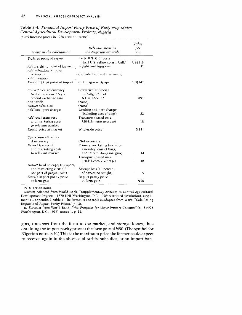
82 FINANCIAL ASPECTS OF PROJECT ANALYSIS
Table 3-4. Financial Import Parity Price of Early-crop Maize,Central Agricultural Development Projects, Nigeria(1985 forecast prices in 1976 constant terms)
ValueRelevant steps in per
Steps in the calculation the Nigerian example ton
F.o.b. at point of export F.o b. U.S. Gulf portsNo.2 U.S. yellow corn in bulka US$116
Add freight to point of import Freight and insurance 31Add unloading at point
of import (Included in freight estimate)Add insurance
Equals c.i.f. at point of import C.i.f. Lagos or Apapa US$147
Convert foreign currency Converted at officialto domestic currency at exchange rate ofofficial exchange rate N I = US$1.62 N91
Add tariffs (None)Deduct subsidies (None)Add local port charges Landing and port charges
(including cost of bags) 22Add local transport Transport (based on a
and marketing costs 350-kilometer average) 18to relevant market
Equals price at market Wholesale price N 131
Conversion allowanceif necessary (Not necessary)
Deduct transport Primary marketing (includesand marketing costs assembly, cost of bags,to relevant market and intermediary margins) - 14
Transport (based on a350-kilometer average) - 18
Deduct local storage, transport,and marketing costs (if Storage loss (10 percentnot part of project cost) of harvested weight) - 9
Equals import parity price Import parity priceat farm gate at farm gate N90
N Nigerian naira.Source: Adapted from World Bank, "Supplementary Annexes to Central Agricultural
Development Projects," 1370-UNI (Washington, D.C., 1976; restricted circulation), supple-ment 11, appendix 2, table 4. The format of the table is adapted from Ward, "CalculatingImport and Export Parity Prices," p. 10.
a. Forecast from World Bank, Price Prospects for Major Primary Commodities, 814/76(Washington, D.C., 1976), annex 1, p 12.
gins, transport from the farm to the market, and storage losses, thusobtaining the import parity price at the farm gate of N90. (The symbol forNigerian naira is N.) This is the maximum price the farmer could expectto receive, again in the absence of tariffs, subsidies, or an import ban.

PRICING PROJECT COSTS AND BENEFITS 83
Figure 3-1. Diagrammatic Derivation of Import Parity Priceof Early-crop Maize, Central Agricultural Development Projects, Nigeria(1985 forecast prices in 1976 constant terms)
WHOLESALE PRICEAT INLAND MARKET
Transportto inland market + N 18
Local port charges + N22 - N14 Primary marketing
(Price convertedat official exchange
rate of N = US$1.62) - N 18 Transportfrom project
C.I.F. N91 to marketLAGOS OR APAPA US$14
Freight - N9 Storage lossand + US$31
insurance
F.O.B. US(116IMPORT PARITY PRICEU.S. GULF PORTS AT FARM GATE
N Nigerian naira.US$ U.S. dollars.Source: Same as table 3-4.

t~~~~~~~ ¢I1 i'h. 4 .4*
|rs ~ ~ --,* .-.
L :\
A* F - 3T
_. ^t ... *.

4
Farm Investment Analysis
ONCE MARKET PRICES have been determined for those items that enter thecost and benefit streams, this information must be arranged in "pattern"accounts to begin the assessment of the effects a proposed project willhave on the farmers, public and private enterprises, and governmentagencies that will participate in project implementation. These accountsare central to the financial analysis of agricultural projects; they arealways based on market prices.
Although we will touch on the essential elements of financial analysis,much more could be taken up here. Just how elaborate the financialanalysis must be for a particular project will depend on the complexity ofthe project. Most agricultural projects will call for a financial projectionbased on at least one pattern farm plan that is assumed for participatingfarmers. This pattern (or model) farm plan projects resource use andincome flows for a group of similar farms participating in the project.The financial projections for the private and public firms or projectentities may be quite summary in nature for a simply organized project,but a project in which several different firms and project entities areconcerned or one that poses special financial problems may involve amuch more complex analysis. The major accounts needed will be out-lined in this chapter and in chapters 5 and 6, and pattern formats
Facing page: Setting out for the field in Paraguay.
85

86 FINANCIAL ASPECTS OF PROJECT ANALYSIS
suggested. This will enable the project analyst to proceed with the con-fidence that he is preparing an acceptable financial analysis. For morecomplex projects, especially those projects involving more complex pub-lic or private firms with specialized cost, revenue, or financing situations,the project analyst will have to move beyond what is discussed here.Agricultural project analysts may want to turn for more technical help tofinancial analysts or accountants, just as they would turn to agricultural-ists or livestock technicians for their particular expertise. Many financialanalysts and accountants, however, will not be familiar with methodolo-gies of agricultural project analysis or with the particular analyticalneeds of the financial aspects of these projects, so even financial analystsand accountants may find that the following discussion may help themrespond to a request for assistance.
Objectives of Financial Analysis
Six major objectives for financial analysis occur in analyzing agri-cultural projects.
Assessment of financial impact
The most important objective of financial analysis is to assess thefinancial effects the project will have on farmers, public and privatefirms, government operating agencies, and any others who may be par-ticipating in it. This assessment is based on an analysis of each partici-pant's current financial status and on a projection of his future financialperformance as the project is implemented. Detailed financial projec-tions are needed for this analysis.
Judgment of efficient resource use
The overall return of the project and the repayment of loans extendedto individual enterprises are important indicators of the efficiency ofresource use. For management especially, overall return is importantbecause managers must work within the market price framework theyface. Farm investment analysis and financial ratio analysis provide thetools for this review. Project analysts and others concerned with deci-sions on policies for national economic growth and development willhave to look beyond the financial analysis-at market prices-and form ajudgment about the effects of the project on real resources for the econ-omy as a whole. In chapter 7 we take up this issue in the discussion of howto determine economic values.
Assessment of incentives
The financial analysis is of critical importance in assessing the incen-tives for farmers, managers, and owners (including governments) who

FARM INVESTMENT ANALYSIS 87
will participate in the project. Will farm families have an incrementalincome large enough to compensate them for the additional effort andrisk they will incur? Will private sector firms earn a sufficient return ontheir equity investment and borrowed resources to justify making theinvestment the project requires? For semipublic enterprises, will thereturn be sufficient for the enterprises to maintain a self-financing capa-bility and to meet the financial objectives set out by the society?
Provision of a sound financing plan
A principal objective of the financial analysis is to work out a plan thatprojects the financial situation and sources of funds of the various projectparticipants and of the project itself. The financial plan provides a basisfor determining the amount and timing of investment by farmers and forsetting repayment terms and conditions for the credit extended to sup-port the investment. It provides the same basis for an assessment of theinvestment plans and debt repayment capacities of public and privatefirms participating in the project. Finally, for the project as a whole, thefinancial plan is the basis for determining the amount and timing ofoutside financing-whether from the national treasury or from interna-tional sources-and for establishing how rapidly the borrowed resourcesshould be repaid. The estimated effect of inflation on both revenues andcosts should be taken into account in making this assessment.
Coordination of financial contributions
The financial plan allows the coordination of the financial contribu-tions of the various project participants. The coordination is made on thebasis of an overall financial projection for the project as a whole. Itaddresses itself to such questions as whether the availability of resourcesfrom the treasury or international agency is matched with farmers'investment capacities and available funds for investment and operatingexpenses as well as with the timing of expenditures for project invest-ments such as feeder roads and irrigation structures and for workingcapital needed for stocks in processing industries and the like.
Assessment of financial management competence
On the basis of a projection of the pattern financial accounts, especiallyfor the larger firms and project entities, the analyst can form a judgmentabout the complexity of the financial management the project will re-quire and about the capability of those who will manage the project'simplementation. And from this assessment, the analyst can then judgewhat changes in organization and management may be necessary if theproject is to proceed on schedule and what specialized training may beadvisable.

Table 4-1. Differences between Farm Income Analysis, Funds Flow Analysis,
and Farm Investment Analysis
Item Farm income analysis Funds flow analysisa Farm investment analysisb
General objective Check current Check farmer's liquidity Check attractivenessperformance of farm of additional investment
Period usuallyanalyzed Individual years Loan repayment period Useful life of investment
Prices used Current prices Current prices Constant prices
Treatment Annual depreciation Cash purchases Initial investment, residual
of capital charge and sales value
00 Off-farm income Excluded Cash portion included Cash and noncash included
Home-consumedfarm production Included Excluded Included
Performance Return to capital and Cash available to farm Return to additionalcriteria labor engaged on farm family resources engaged
Time value Undiscounted Undiscounted Discounted
Performance Profit as a percentage Cash surplus or deficit Net present worth, internal
indicators of net worth, family rate of return, benefit-cost ratio,income net benefit-investment ratio,
net benefit increase
Source: Schaefer-Kehnert (1980).a. Also called sources-and-uses-of-funds analysis.b. Benefit-cost analysis of on-farm investments.
FARM1 INVESTMENT ANALYSIS 89
Preparing the Farm Investment Analysis
The starting point for both the financial and the economic analysis ofan agricultural project is generally a group of investment analyses ofpattern or model farms, based on budgets for individual pattern farms.These pattern farm budgets compare the situation with the project tothat anticipated without the project for the duration of the project. Theyenable the analyst to form a sound judgment about the likely benefit tofarmers of participating in an agricultural project and about the incen-tives for farmers to do so.
Farm investment analysis is the topic of this chapter. This analysis issimilar to, and sometimes confused with, farm management analysesdone by agricultural economists, which may be distinguished as farmincome analysis and funds flow analysis. The differences are summarizedin table 4-1.
Farm income analysis is generally used to evaluate the performance ofa farm in a particular year. Its objective is to help improve the manage-ment of the farm. Current prices are used, and a depreciation allowanceis included to account for that portion of longer-term capital investmentused up in the year being considered. Noncash items such as home-consumed production and payments in kind are included. Off-farm in-come and expenditure are excluded because the analysis is intended toevaluate the performance only of the farm itself. The analysis provides anestimate of the return to capital invested and to the farmer's labor, andthis may then be compared with the return to alternative croppingpatterns or to off-farm opportunities.
Funds flow analysis, also called sources-and-uses-of-funds analysis, isused to determine a farmer's liquidity in an analysis of his credit situa-tion. Only cash iterns, including purchase and sale of capital goods, enterthe analysis. Off-farm cash income and expenditure are included, buthome-consumed production is not. The analysis shows the cash availableto the family over a period of time.
Farm investment analysis, in contrast, is undertaken to determine theattractiveness of a proposed investment to farmers and to other partici-pants, including the society as a whole. It projects the effect on farmincome of a particular investment and estimates the return to the capitalengaged. It follows the principles of discounted cash flow analysis (dis-cussed in detail in chapters 9 and 10). The analysis is projected over theuseful life of the investment. The initial investment is shown at thebeginning of the projection, and a residual value at the end. In general,the analysis is cast in constant prices, although allowance may have tobemade for inflation. Off-farm income is included. Even though we use theterm "cash flow," noncash elements enter the projection, includinghome-consumed production and payments and receipts in kind. (Theterm was first applied to industrial investments, in which noncash ele-ments are less common.) When doing farm investment analysis, some

90 FINANCIAL ASPECTS OF PROJECT ANALYSIS
elements of funds flow analysis are often incorporated to enable theanalyst to assess the farmer's liquidity and his credit use. Those who wishto pursue farm income analysis or funds flow analysis in relation toproject analysis may refer to standard farm management texts such asHarsh, Connor, and Schwab (1981) and Kay (1981). Those who wantmore detail about the application of farm budgets to project analysismay consult Brown (1979).
Pattern farm investment analysis that includes farm budgets should beprepared for almost every agricultural project. Although agriculturalproject analyses that do not have farm budgets are used, it is increasinglyaccepted that farm budgets are an extremely desirable, if not essential,part of project analysis. The benefit stream of an agricultural project maybe built up simply by multiplying the total area to be planted by theexpected yield, essentially treating the whole area as one undifferenti-ated farm. If this is all that is done, it may hide crucial information aboutthe effects of the project on individual farmers and obscure underlyingunrealistic assumptions. Even when the project involves only a publicsector undertaking, a farm budget is likely to be necessary to test thefeasibility of the cropping pattern and the financial viability of theenterprise.
The purpose in preparing farm investment analyses for a project is notto take a sample of the farms in the project area. Rather, it is to selectmajor farm types expected to participate and to look at the impact of theproject on them. These farm investment analyses are usually projectionsfor the life of the project, often twenty to twenty-five years, not for just asingle year. The analyst will want to examine the cropping pattern andperhaps to diagram it; to determine the labor that will be required iffarmers are to participate in the project and perhaps to prepare a month-by-month labor budget showing requirements and the availability offamily labor; to look at production and inputs; and, finally, to prepare afarm budget in the detail needed for understanding and evaluating theeffects of the project on the income of participating farmers. From these,the analyst can assess the financial effect of the proposed project ontypical farms-both to judge incentives for participation and to deter-mine whether national policies on minimum incomes for project partici-pants are being met.
Farm investment analyses and farm budgets can of course be preparedfor farms of any size. The problems of analyses for smaller farms are thefocus here, since many, if not most, agricultural projects in developingcountries will be directed toward smallholders whose families consumea large part of the food they produce.
Large commercial farms and plantations, however, whether publiclyor privately held, are more like other business enterprises than they arelike small, family-operated farms. Projected accounts for these largeagricultural undertakings are probably more appropriately cast in for-mal financial statements such as those of the agricultural processingindustries discussed in chapter 5.
In considering small farms, the analyst will be particularly concernedwith the effect of the project on the total income of the farm family. The

FARM INVESTMENT ANALYSIS 91
aspects of the small farm as a family unit and as a business firm must beclearly understood and appreciated. These will differ from society tosociety, and the project analyst should either know the society wellenough to anticipate the farmers' response or be advised by others whodo. One must assess the attitude of the family to proposed croppingpatterns that involve more days of labor, to patterns that increase cashcrop output and reduce food crop production below household require-ments, to patterns that change the work responsibilities of men andwomen, and to patterns that require the family to run a considerablemarket risk. Farmers are price responsive, of course; the extensive re-search has amply confirmed this (Krishna 1967). But farmers live in aparticular cultural and risk environment, and project analysts must takethis environment into account when they project their pattern farminvestment analyses.
Backed by this understanding of the particular cultural environment,the analyst will prepare the farm investment analyses as realistically aspossible to determine what the family gains by participating in theproject. The projection must be based on a specific package of techno-logical innovation. The effectiveness of the proposed new technology onsmall farms must be realistically assessed, and the technologicalassumptions must be checked to ensure that they reflect on-farm condi-tions and not those of an experiment station. The analyst must form ajudgment about how rapidly farmers will be willing to adopt new prac-tices. The farm investment analysis should confirm that adoption of anew technology will really be financially worthwhile, for farmers canrespond to financial incentives only when it is truly remunerative forthem to do so. The analyst must determine how much credit will stimu-late farmers to adopt new practices and must assess how risky a newtechnology is and how variable the farm income may be under theproject. The analyst will want to test the effect of risk on family incomeby determining what happens if yields fall below expectations or if pricesare lower than anticipated and by undertaking similar sensitivity tests.Through such tests a margin to allow for bad years can be built into thefarm plan.
Although in agricultural projects the analyst generally looks atbudgets for entire farms, partial budgeting techniques can be used forundertakings that involve only a relatively minor change in the farmorganization. To do this, one looks at the marginal cost (including oppor-tunity cost) of adding a production activity and compares it with themarginal increase in benefit that the new activity will bring. Partialbudgets are an effective tool for helping to search out the best combina-tion of production activities. Brown (1979) discusses their use in somedetail. In most projects, however, we expect rather substantial changesover a prolonged period, and under these circumstances it is better toproject whole farm budgets. Then the total effect of the project on familyincome can be better assessed.
The information on which the project analyst will base his farm invest-ment analysis will come from many sources. Project analysts will have torely heavily on their professional colleagues to determine a sensible

92 FINANCIAL ASPECTS OF PROJECT ANALYSIS
cropping pattern and livestock activity for a proposed project, the outputthat may be expected, the inputs that will be required, and the relevantprices for products. The project analyst will want to pay particularattention to the realism of the estimates provided by the agriculturalistsand livestock specialists he consults. Unrealistic assumptions aboutyields, input levels, or rates of farmer acceptance and, hence, of buildupin project benefits will negate the best of project analyses.
The analyst will certainly want to visit the site of the proposed projectand typical farms that will be included. Nothing substitutes for thefirsthand knowledge that being there brings.
A crucial source of information in every agricultural project is thefarmers themselves. Only through interviews with farmers can a projectanalyst reach a valid conclusion about the realism of his farm investmentanalysis. The project analyst will want to interview farmers about theirpresent cropping patterns, labor requirements, use of inputs, and themarket prices actually received and paid. He will want to gain a senseabout the farmers' willingness to participate in the project were it toproceed. In a project area or on a similar site some farmers often arealready using a proposed new technology. It is most important that thesefarmers be interviewed to tap their experience. The analyst will want toknow the yields the farmers actually have realized with the new technol-ogy, the inputs they actually must employ, and their general commentson the new technology and cropping pattern proposed for the project.The analyst will want to assess the labor requirements farmers havefound necessary to use the new technology.
Interviewing farmers is an art in itself, and only a few comments can bemade here. The information farmers give will usually be contradictory,but out of a group of interviews the project analyst can gain a sense offeasible technological and financial relations. Farmers will have to beinterviewed in the field, not in the office. The analyst will have to knowthe local measurements and not expect everything to be reported neatlyon a unit basis. The analyst or one of his staff should probably conductthe interviews alone or with very few other people around. Great careshould be taken to establish a good atmosphere in the interview so thatfarmers are not overawed by the analyst's presence; farmers should alsoknow that the information they give will not be used for tax purposes. Aformal questionnaire may be helpful, especially if much information is tobe collected by assistants, but any questionnaire should be carefullypretested in the field before use. It may be better for the analyst or hisassistants to fill in the questionnaire only after the interview is completeand the interviewer has left the farmer. In any event, before the inter-views the analyst should have formed a clear idea about the informationhe needs, perhaps in the form of a list of questions, so that criticalinformation will not be overlooked. Questions put to farmers should beas specific as possible. Most information gathered should relate to actualexperience, perhaps in the last cropping season. Questions abouthypothetical situations should be avoided to the extent possible. The

FARM INVESTMENT ANALYSIS 93
very nature of seeking information about a proposed project will, how-ever, of necessity involve many "what if" kinds of questions.
Cropping patterns are usually based on the judgment of the agricultur-alists and livestock specialists working with the project analyst. Theirjudgment, in turn, will be based on their familiarity with the agricultureof the area, on research results and the results of pilot projects-perhapsundertaken especially as part of the project preparation-and on theirknowledge of the farmers who will participate in the project. In mostinstances, experienced technicians can propose realistic patterns close tothe optimum, but sometimes linear programming may be used as a moreformal methodology to optimize cropping patterns. Linear program-ming has been applied in preparing agricultural project analyses but isnot regularly used either in national planning agencies or in inter-national lending agencies. It is a complex methodology that requiresmore formal input-output data than does simple budgeting, and in prac-tice it requires computers. There are serious methodological limitationsto the use of linear programming for agricultural project analysis: prob-lems of dealing with risk, farmers' cultural traditions, variability of soilswithin farms, water availability in different areas of a farm, and otherfarm-level variations. Even so, when preparing a project for an areawhere there is inadequate experience to rely on in forming subjectivelydetermined cropping patterns or when dealing with very complex pat-terns, the project analyst may want to consult specialists in linear pro-gramming for assistance. In these cases, the project preparation takes onsome of the character of a research effort. Because it is a well-knownmethodology widely used in farm management research, many agri-cultural colleges have staff familiar with linear programming.
In most agricultural projects, about half a dozen or so pattern farminvestment analyses will suffice, but generalization about this is danger-ous. The number of pattern farm analyses depends entirely on the com-plexity of the project. The analyst will want a pattern farm investmentanalysis for each major group of soil and water conditions in the projectarea and for each major difference in the size of holdings. Of course, eachmajor cropping pattern or livestock activity will require a separate farminvestment analysis. Remember that the objective is an indication of theeffect of the project, not some kind of rigorously drawn, random sample.In practice, the number of farm budgets prepared for any given projectanalysis is a tradeoff between the complexity of the proposed project andthe availability of staff to prepare the investment analyses.
Each farm investment analysis will be the result of careful consulta-tion with technical specialists and interviews with farmers. Just as it isnot possible to generalize about how many pattern farm budgets will benecessary, neither is it possible to generalize about how many interviewswith farmers will be needed. Thorough preparation of a complex projectmay require twenty-five to fifty or even more interviews to provide theinformation for each farm analysis. But a simpler project that will use abetter-known technology may require only half a dozen to a dozen inter-

94 FINANCIAL ASPECTS OF PROJECT ANALYSIS
views for each pattern farm budget. A group doing an appraisal of aproposed project would probably interview fewer farmers than wasnecessary in the initial project preparation. Each situation will have tobe judged by itself in the light of how confident the analyst needs to beabout the project analysis, how complex the project is, how well knownthe technology is, and how available are staff for project preparation.
Similar considerations apply in deciding the level of detail necessaryin a farm investment analysis. Any farm investment analysis is intendedto improve the decisionmaking for a project. It is, of necessity, an ab-straction. This imprecision is forced on us by the very fact that we mustpredict future events, but it also arises from the question of just howmuch detail is necessary. In every farm investment analysis, the projectanalyst will reach a point at which further elaboration or further detailwould make such a marginal contribution to the investment decisionthat it is not worth the time. Just when that point is reached will varyfrom project to project according to the circumstances of the project andthe circumstances of the decisionmaking process.
It is easy to conceive of a set of pattern farm investment analyses thatwould be so enormously detailed and have so many different budgetsthat the process would quickly become bogged down in detail. Because ofstaff limitations and because of the approximate nature of the underlyingdata, it is better to hold both the number of pattern farms and the level ofdetail to the minimum that will serve to lay out clearly the major pointsabout the project.
The project analyst will have to determine how best to present hisinformation so that those who must review his work and make decisionsabout the project can work efficiently and yet have the information theyneed. The major entries, the level of detail, and the like will vary fromproject to project. Some of the elements given in separate tables in theillustrative examples in this chapter may be better combined in thetables that present a particular project. In many project reports, only asummary of background information, plus a detailed farm budget, willbe needed. Other, more detailed tables can be included in annexes or in aseparate volume of background information reproduced in limited quan-tities and circulated only to those most interested in the project. Thiskind of additional data can even be kept in a separate project informationfile that can be made available to anyone seriously interested. (In theParaguay report used as an example in this chapter, the analyst pre-sented his farm investment analysis in four annex tables and collectedthe supporting information in a separate project information file.)
What we will present here is a pattern format that includes the featuresmost commonly of significance in agricultural project analysis. Thispattern format uses a terminology generally accepted by both farmmanagement specialists and accountants. In using the format, theanalyst will have to determine for himself, for each project in his charge,exactly how much detail is necessary to support the analysis and exactlyhow this detail is best reported to facilitate decisions about the particu-lar project.

FARM INVESTMENT ANALYSIS 95
Elements of Farm Investment Analysis
The principal elements of farm investment analysis are outlined in thissubsection and are listed in table 4-2. A flow chart for preparing theanalysis is given in figure 4-1. Not every element will be necessary inevery analysis, and the means of presenting the elements will vary fromproject to project according to circumstances.
The most important elements of a farm investment analysis can beillustrated by an example adapted from the Paraguay Livestock andAgricultural Development Project. (Tables that illustrate particular ele-ments of the analysis are noted in table 4-2.) The project is to increaseagricultural production, productivity, and income on some 940 livestockfarms and some 3,000 mixed farms, mostly small, through on-farm in-vestments supported by credit, technical assistance, feeder roads, andmarket improvement. Most of the important aspects of preparing a farminvestment analysis are touched on in this example, but it is clear that nosingle example can cover every possibility. Each project analyst willwant to build on the illustrative tables that outline this one example forthe purposes of his own project analysis. As in all accounts, the objectivesof the farm investment account determine its content and format.
Accounting convention for farm investment analysis
Because farm investment analysis follows the principles of discountedcash flow, it is convenient to adopt an accounting convention that iscongruent with those principles. [This convention has been called "time-adjusted" by Schaefer-Kehnert (1980), who has elaborated its use.] Thediscounting process used in discounted cash flow analysis implicitlyassumes that every transaction falls at the end of the accounting period.It is desirable that the farm investment analysis match this assumption.This is simply accomplished if we consider the initial investment to takeplace at the end of year 1 of the project, regardless of whether it willactually take a full year or only a few weeks. Year 2, then, is the firstaccounting period in which increases in operating cost and incrementalbenefits occur. Thus, the dividing line between the end of the initialinvestment period and the beginning of the incremental productionoperations coincides exactly with the dividing line between years I and 2of the project. (Some analysts accomplish much the same result byconsidering investment to fall in year 0, but this gives rise to problemswhen cash flows are aggregated.) Considering that preparing a farmplan, making a loan, constructing or purchasing investment items, andpurchasing new inputs can take at least several months to a year, reserv-ing year 1 for investment is not unrealistic. Doing so, however, is notdictated by real events but by the accounting convention.
If all transactions are considered to fall at the end of the accountingperiod, then we must allow for the availability of the needed operating

96 FINANCIAL ASPECTS OF PROJECT ANALYSIS
Table 4-2. Principal Elements of Farm Investment Analysis
IllustrativeElement table
Farm resource useLand use 4-4(Land use calendar) (Figure 4-2)Labor use
Annual labor requirement by crop operation,by crop for I hectare 4-5
Labor distribution by crop and month, per hectare 4-6(Labor use diagram) (Figure 4-3)Labor requirement by crop and month 4-7Hired labor by crop and month 4-8Off-farm labor Not illustrated
Farm productionCrops and pasture
Yield and carrying capacity 4-9Crop and pasture production 4-10
LivestockHerd projection 4-27Herd composition, purchases, sales 4-11Herd productivity 4-28Feeding period and daily ration 4-29Feed requirement and production 4-30Yield per animal Not illustrated
ValuationFarm-gate prices 4-12Value of production
Crops 4-13Livestock
Incremental residual value 4-14
Farm inputsInvestment
Physical 4-15Foreign exchange component Not illustratedValue of investment 4-15
Operating expenditureCrop 4-16Livestock
Incremental working capital 4-17
Farm budgetWithout project 4-18With project
Net benefit before financing 4-19Debt service 4-24Net benefit after financing 1 4-19Cash position 4

Figure 4-1. Flow Chart for Farm Investment Analysis
(4-15)- 1
Annu.al labor
requmement per hectare_
by crop and operation
L,cpanordsnbto Labor requirement Hired laborcrmnab npadmonth, bY month _by crrp and month reiua m
per hectare (4-7J , 4-8) (414
Land use _ Oeang Ic
(4-4) In1n ta xf4nd2tue 1 sol
Yedand carrying L (4-2nd4s)rel capacity _ pduti n I
(4-9) (4-1 0) |Vleo|
Parm-gate pnces / \, _ pnrodcucon -(4-12)
(4 (-3
Y.eld per a-mal m e |ad rrd e.o |1l (not illustrated) an l h o
| Feeding penod | and daily ration '5 a d 1 Hr opszon, |
(4-29) 1 Ddj =
Of-a m mcoe(not d(u-tratedl I
a. Numbers in parentheses refer to the illustrative tables in this chapter.

98 FINANCIAL ASPECTS OF PROJECT ANALYSIS
expenditure at the beginning of the cropping season. This is accom-plished by incorporating in the analysis an entry for incremental work-ing capital at the end of the preceding year. The amount of the workingcapital needed is related to the farming system being analyzed. If a singleannual crop is produced, then nearly all the operating expenditure willbe needed at the beginning of the crop year. But if two crops are to beproduced in succession, only the operating expenditure for the first cropneed be on hand at the beginning of the crop year, since there will be aharvest during the year that will provide proceeds to replace the inputsupplies needed before the second crop is harvested. Thus, only half thetotal annual operating expenditure need be on hand at the beginning ofthe year. The incremental working capital needed (either an increase or adecrease) at the beginning of the year, then, is entered at the end of theyear preceding the year when it will be expended for production. A set ofrecommended adjustments in incremental operating expenditure toobtain incremental working capital is given in table 4-3. Introducing anincremental working capital stream reflects real resource use. When aninvestment is undertaken, short-term inputs such as seed, fertilizer, feed,and the like must be on hand. They are replaced from the proceeds of theharvest or livestock sales during the year and are again on hand forproduction in the following year. If operations are to expand the nextyear, then stocks of inputs for production must be increased, and this willbe reflected in another incremental working capital entry. Since theincremental working capital is entered separately, it will easily be in-cluded in the total investment shown when the farm budget is preparedand will not be inadvertently overlooked. At the end of the project, theincremental working capital for each year is added together algebra-ically and taken out of the project as part of the residual value. Thus,including incremental working capital in the accounts does not result indouble counting.
One practical outcome of this accounting convention is that operatingexpenditures and benefits in year 1 generally remain the same as theywere without the project. In some cases new investment might require anincrease in operating expenditure in year 1, even though production
Table 4-3. Incremental Working Capital as a Percentageof Incremental Operating Expenditure
Item Percent
Tree crops (slowly maturing,one harvest season) 100
Annual cropsOne season 80-100Two seasons 40-60
Continuous cropping and continuouslyproducing livestock enterprises 20-40
Source: Schaefer-Kehnert (1980).

FARM INVESTMENT ANALYSIS 99
would not be affected until year 2. In other instances, both operatingexpenditures and production might actually decrease-as might happenif new irrigation canals were to be constructed, disrupting farming op-erations. In laying out the farm investment analysis, however, it is usu-ally considered that working capital is not freed as a result of the invest-ment so that the layout of the farm budget can be simplified. If this werenot done, both data for the case without the project and data for a"preproject" year or "year I" would be needed to accommodate thedecision rule that working capital be a proportion of the increase ordecrease in the operating expenditure for the following year.
Showing working capital as a separate entry facilitates determininghow much short-term credit may be needed by the farmer. A judgmentmay be made about whether the farmer will have savings from which tofinance increased working capital or whether some proportion or all willhave to be covered by extending the farmer a short-term loan, which thencan be incorporated into the financing section of the farm budget.
The accounting convention adopted here is not much different fromthat most commonly used by project analysts. The most important dif-ference is the rule of reserving year 1 for investment only and assumingthe investment to fall at the end of the year. It is more common to includeinvestment in year 1 but to assume that it will occur at the beginning ofthe year, even though the discounting process assumes it falls at the endof the year. Production is then assumed to be increased in year 1, anassumption that leads to an overestimate of the rate of return on thecapital used. It also leads to a considerable overestimate of the farmer'sincome in the early years of the project and, hence, to an underestimate ofhis need for both long-term and short-term credit. The other differencebetween the accounting convention adopted here and that most com-monly used by project analysts is only a matter of completeness. It is easyinadvertently to omit or underestimate working capital unless suchcapital is included in the convention. This convention for working capitalleaves the crop year intact and therefore facilitates the supporting tech-nical projections.
Farm resource use
Once the agronomists, livestock technicians, and other technical spe-cialists have determined the components of a proposed farming systemfor a pattern farm, the analyst may proceed to prepare the farm invest-ment analysis.
LAND USE. The first step is to determine what the land use on the farmwill be. The land use for the Paraguay project is given in table 4-4. Notethat the crop year is taken to extend from July of one calendar year toJune of the next, since this arrangement makes the break in the year comeduring the Paraguayan winter season, when there are the fewest crops inthe ground. The total farm area is 20.0 hectares, divided into cultivatedarea, pasture, forest, and a house plot. (Throughout the text of this chapter,

100 FINANCIAL ASPECTS OF PROJECT ANALYSIS
Table 4-4. Land Use, 20-Hectare Mixed Farm, Livestockand Agricultural Development Project Model IV, Paraguay(hectares)
With projectType of use Withoutand cropa project Year 1 2 3 4 5 6-20
Cultivated areaMaizeb 0.5 0.5 0.5 0.5 0.5 0.5 0.5Maniocb 1.0 1.0 1.0 1.0 0.5 0.5 0.5Beans 0.5 0.5 0.5 0.5 0.5 0.5 0.0Cotton 2.0 2.0 2.0 2.0 2.2 2.5 3.0Soybeans 0.0 0.0 1.0 1.0 2.2 2.5 3.0Sunflowerc 0 0 0.0 2 0 2.0 2.2 2.5 3.0Total 4.0 4.0 7.0 7.0 8.1 9.0 10.0
Total croplandd 4.0 4.0 5.0 5.0 5.9 6.5 7.0Cropping intensitye 1 0 1.0 1.4 1.4 1 4 1.4 1.4
PastureNatural 10.5 7 0 3 5 0.0 0.0 0.0 0 0Improved 0.0 3.5 7.0 10.5 10.5 10.5 10.5Total 10.5 10.5 10 5 10.5 10.5 10.5 10.5
Forest 5.0 5.0 4.0 4.0 3.1 2.5 2.0
House plot 0.5 0.5 0.5 0.5 0.5 0.5 0.5
Total farm area 20 0 20.0 20 0 20.0 20.0 20.0 20.0
Source: Adapted from World Bank, "Staff Appraisal Report: Paraguay-Livestock andAgricultural Development Project," 2272-PA (Washington, D.C., 1979; restricted circula-tion), annex 1, table 17.
a. Operated by one family with six members and a work potential of 70 work days amonth. A work day is the time (generally eight hours) devoted by one person during one day.
b. Maize and manioc are intercropped.c. Double-cropped after cotton or soybeans. The area given is the area planted in the year
shown.d. Does not include second crop area, in this case the area planted in sunflower.e. Cropping intensity is determined by dividing the total cultivated area by the total
cropland.
the most common or generalized categories from the pattern tables willbe shown in italic type. These items would be considered in any farminvestment analysis. In all tables the generalized analytical frameworkapplies, but in some the categories are all specific to the projectanalyzed.)
The land use, in accord with the accounting convention adopted,would remain unchanged in year I, exccpt for establishment of improvedpasture that is part of the investment. In year 2, in which the proposedcropping pattern calls for sunflower to be introduced and to be double-cropped after either cotton or soybeans (depending on the year), both thetotal cultivated area and the total cropland are shown. The total culti-vated area is the total area planted in crops, whereas the total cropland isthe area available to cultivate. When the total cultivated area is dividedby the total cropland, the cropping intensity is obtained. In year 2, for

FARM INVESTMENT ANALYSIS 101
example, the cropping intensity is 1.4 (7.0 -- 5.0 = 1.4). Many analystsprefer to report cropping intensity in percentages, so this would bereported as 140 percent. One check of the feasibility of the croppingpattern is the intensity. The analyst should be cautious about accepting acropping pattern that has a very high cropping intensity or one that ismarkedly different from the pattern existing in the area. Farmers maywell have good reasons for not driving up the intensity.
Many analysts also like to devise a cropping diagram, such as thatgiven in figure 4-2, and this should be subdivided to indicate any existingfarm plots. Such a diagram is usually drawn up only for the full-development situation. The diagram indicates the area to be devoted toeach category of land use and each crop. In the case of our example, itextends over two years to show that the seasonal timing of the cotton-sunflower-soybean rotation occurs on one plot in one year and on anotherin the next. Checking vertically at any one time, we can be sure thecropping pattern does not call for more area than the farm has. Checkinghorizontally, we can determine when each crop must be planted andwhether enough land will be available at the proper season. The left andright sides of the boxes showing the area to be planted in each crop areslanted to indicate the planting and harvest time necessary for each crop.Examining the cropping diagram can help determine if there will beadequate time between crops to prepare the land.
Figure 4-2. Land Use Calendar for Project Years 6-20,20-Hectare Mixed Farm, Livestock and AgriculturalDevelopment Project, Paraguay
20 Forest19 (2.0 ha) 61817 -16 -15 -14 - Improved13 - pasture 5 D
1, 12 (10.5 ha)11-10_ Sun-9 -Sunflower flower8_ (3.0 ha) (3.0 ha)7-6 Soybeans Cotton 45 _ //(3.0 ha) (3.0 ha) Cropland
34 _ / Cotton Sunflowerl Soybeans (7.0 ha)332 (3.0 ha) (3.0 ha) (3.0 ha) /I Maize an manioc (1.0 ha) _ House 2O , -< ~plot IJIAISIOINIDIJIFIMIAIMIJIJIAISIoINIDIJIFIMIAIMIJ (0.5 ha)
Montha
ha Hectares.Source: Table 4-4.a. Crop year is from July to June.

102 FINANCIAL ASPECTS OF PROJECT ANALYSIS
LABOR USE. A second aspect of the farm resource use is labor. Todetermine the labor the farm will require, we need to know the labor usedto cultivate a hectare of each crop in each project year. It is desirable tobe able to see this in two forms, by operation and by month. Table 4-5shows the annual labor requirements for 1 hectare by crop and operationfor the Paraguay project example. It includes the labor required not onlyfor the various crops to be produced, but also for the pasture. The laborunit is a work day, the time (generally eight hours) devoted by one personduring one day. The labor requirement for crops drops sharply betweenyears 1 and 2 because of the introduction of draft animal power. In thecase of pasture, the labor requirement for fencing and seeding is includedin years 1 through 3. In the Paraguay model, other activities of pastureestablishment are to be undertaken by a contractor, so there will be nocall for labor from the farmer. If, however, labor for establishing someother kind of improvement were expected, such as farmers' digging theirown tertiary canals in an irrigation project, then this should be includedin the labor requirement.
Table 4-5. Annual Labor Requirement per Hectareby Crop and Operation, 20-Hectare Mixed Farm, Paraguay Project(work days)
With projectWithout
Crop and operation project Year 1 2 3 4 5 6 7-20
CropsMaize
Land preparation and planting 22 22 11 11 11 11 11 11Cultivationa 9 9 2 2 2 2 2 2Harvesting 28 28 28 31 31 33 33 36Total 59 59 41 44 44 46 46 49
ManiocLand preparation and planting 14 14 10 10 10 10 10 10Cultivationa 27 27 15 15 15 15 15 15Harvesting 19 19 19 21 21 23 23 25Total 60 60 44 46 46 48 48 50
BeansLand preparation and planting 24 24 19 19 19 19 19 19Cultivation 10 10 4 4 4 4 4 4Harvesting 20 20 20 22 22 22 22 22Total 54 54 43 45 45 45 45 45
CottonClearing 8 8 8 8 8 8Plowing 18 18 3 3 3 3 3 3Harrowing (2 times) J 2 2 2 2 2 2Seeding 4 4 1 1 1 1 1 1Thinning 6 6 6 6 6 6 6 6Cultivation (3 times) 30 30 3 3 3 3 3 3Spraying (5 times) 10 10 10 10 10 10 10 10Harvesting 37 37 43 43 46 46 49 49Drying, packing, marketing 4 4 4 4 4 4 4 4Total 109 109 80 80 83 83 86 86

FARM INVESTMENT ANALYSIS 103
Table 4-5 (continued)
With projectWithout
Crop and operation project Year 1 2 3 4 5 6 7-20
SoybeansClearing - - 8 8 8 8 8 8Plowing - - 3 3 3 3 3 3Harrowing (2 times) - - 2 2 2 2 2 2Seeding - - I I I I I 1Thinning - - 6 6 6 6 6 6Cultivation (2 times) - - 2 2 2 2 2 2Spraying (2 times) - - 4 4 4 4 4 4Harvesting - - 18 18 20 20 22 22Transport - - 3 3 3 3 4 4Total - - 47 47 49 49 52 52
SunflowerClearing - - 6 6 6 6 6 6Plowing - - 3 3 3 3 3 3Harrowing (2 times) - - 2 2 2 2 2 2Sowing - - 1 1 1 1 1 1Thinning - - 6 6 6 6 6 6Cultivation (2 times) - - 2 2 2 2 2 2Spraying (2 times) - - 4 4 4 4 4 4Harvesting - - 13 14 14 15 15 15Drying, packing, marketing - - 4 4 4 5 5 5Total - - 41 42 42 44 44 44
PastureImproved establishment
Fencing - 7 7 7 0 0 0 0Seeding - 2 2 2 0 0 0 0
Maintenance - - 3 3 3 3 3 3
Note: For the area in various crops, see table 4-4.Source: Adapted from A. 0. Ballantyne, "Paraguay-Small Farmer Credit Component,
Livestock and Agricultural Development Project," working papers on file (Washington,D.C.: World Bank, 1978; restricted circulation).
a. Maize and manioc are intercropped. Hence, during the period when both are growing,the allocation of cultivation time between the two crops has an arbitrary element.
The total labor requirement per hectare for each crop is distributed bymonth in table 4-6. The monthly distribution is most important becausewe must determine not only the total annual labor requirement on thefarm but also its timing to assess whether sufficient family labor will beavailable and, if there is not enough, how much hired labor will beneeded. Although some farm management analysts break down the laborrequirement by week or fortnight, for purposes of project analysis themonthly distribution is sufficient.
On a mixed farm, livestock will also require labor. This may be calcu-lated by determining how much time will be needed per animal unit inthe livestock herd. An animal unit is a measurement of feed demand by aparticular class of animal. (This is discussed in more detail in the appen-dix to this chapter. The total animal units for each year are reported intable 4-11. They are given in that table for the livestock herd that couldexist on 100 model farms to avoid the problem of divisibility that arises

104 FINANCIAL ASPECTS OF PROJECT ANALYSIS
when the increase in large livestock on a small farm is projected. Thus, toobtain the animal units on one farm, the total reported in table 4-11 mustbe divided by 100. We will return to a discussion of this convention in thenext subsection, when we discuss the herd composition.) In the Paraguayexample, it is assumed that each animal unit will require five minutes ofcare a day and that the requirement will be the same each monththroughout the year. The labor requirement is determined on the basis ofthe animal units at the beginning of the year. Using animal units rather
Table 4-6. Labor Distribution by Crop and Month,20-Hectare Mixed Farm, Paraguay Project(work days per hectare)
Crop Jul Aug Sept Oct Nov Dec Jan Feb Mar Apr May Jun Total
MaizeaWithout project, year 1 14 8 0 5 4 28 0 0 0 0 0 0 59Year 2 9 2 0 1 1 28 0 0 0 0 0 0 41Years 3-4 9 2 0 1 1 31 0 0 0 0 0 0 44Years 5-6 9 2 0 1 1 33 0 0 0 0 0 0 46Years 7-20 9 2 0 1 1 36 0 0 0 0 0 0 49
Manioc'Without project, year I 0 0 14 3 3 3 4 3 5 3 3 19 60Year 2 0 0 10 2 2 1 2 2 2 2 2 19 44Years 3-4 0 0 10 2 2 1 2 2 2 2 2 21 46Years 5-6 0 0 10 2 2 1 2 2 2 2 2 23 48Years 7-20 0 0 10 2 2 1 2 2 2 2 2 25 50
Beanswithout project, year I 0 0 0 0 24 5 5 20 0 0 0 0 54Year 2 0 0 0 0 19 2 2 20 0 0 0 0 43Years 3-5 0 0 0 0 19 2 2 22 0 0 0 0 45
CottonWithout project, year I 0 0 8 14 8 19 19 7 20 14 0 0 109Years 2-3 0 0 8 6 8 6 5 8 25 14 0 0 80Years 4-5 0 0 8 6 8 6 5 8 27 15 0 0 83Years 6-20 0 0 8 6 8 6 5 9 28 16 0 0 86
SoybeansYears 2-3 0 0 0 0 13 8 3 2 10 8 3 0 47Years 4-5 0 0 0 0 13 8 3 2 10 10 3 0 49Years 6-20 0 0 0 0 13 8 3 2 11 11 4 0 52
SunflowerbYear 2 2 9 3 13 4 0 0 0 0 0 6 4 41Years 3-4 2 9 3 14 4 0 0 0 0 0 6 4 42Years 5-20 2 9 3 15 5 0 0 0 0 0 6 4 44
PastureImproved establishment
Fencing 2 5 0 0 0 0 0 0 0 0 0 0 7Seeding 0 0 0 0 2 0 0 0 0 0 0 0 2
Maintenance 0 0 0 0 0 0 0 1 0 0 1 1 3
Note: Same as table 4-5.Source: Same as table 4-5.a. See note a, table 4-5.b. Labor requirements for sunflower apply to the year of planting. Thus, in year 2 the
labor requirement is for the crop planted in May of year 2 and harvested in October ofyear 3.

FARM INVESTMENT ANALYSIS 105
than each individual class of animal as the basis for estimating the laborrequirement considerably simplifies the computation and is not un-realistic. In the convention recommended here, for example, closinglivestock figures do not include heifers two to three years old or steerssold during the year, in this case steers three to four years old. Openinglivestock figures, however, omit calves. In reality, closing and openingfigures tend to balance each other, since heifers will be transferred to thebreeding herd throughout the year and surplus heifers and steers will besold throughout the year, whereas calves will be born throughout theyear. Attempting a more precise estimate would only lead to superficialprecision because the error in estimating the daily requirement for laborconsiderably exceeds any gain in accuracy.
Having determined the labor requirement for each crop or animal unitby month, we proceed to calculate the labor requirement for the patternfarm. This is given for the Paraguay example in table 4-7. Here the laborrequired for each crop during each project year is given. The total bymonth and the amount to be provided by family labor and by hired laborare determined. In the Paraguay example, it is assumed that the familyon the pattern farm will have available 70 work days of labor a monthand that any labor requirement in excess of this amount will be suppliedby hired labor. This is a very mechanistic assumption, of course. Not onlywill families vary widely in the labor they have available-even on farmsof quite comparable size and cropping pattern-but families will alsotend to work longer hours in busy seasons and rest in the off-season. Forpurposes of the farm investment analysis, however, this approximationis quite sufficient, given the wide margin of error in the estimates of thelabor requirement in general. In the Paraguay example, table 4-7 showsthat hired labor will be needed on the farm from year 4 onward. By year7, in the peak month of March, about 44 percent of the total laborrequired for cotton and soybeans will have to be hired.
When a labor budget shows a need for hired labor, as this exampledoes, the project analyst must consider carefully whether the labor willbe available in the project area. Totaling the hired labor requirement forthe project as a whole is one of the real advantages of including the laborbudget in the farm investment analysis, since the analyst must thenconsider the realism of the proposed pattern in light of the added hiredlabor that can reasonably be expected to be available in the project area.Postulating 56 additional work days of hired labor in March is one thing;whether such additional labor would be available for an entire proposedproject is another. It may be that a proposed cropping pattern will proveunrealistic in its requirements of additional hired labor, and a lesslabor-intensive cropping pattern must be proposed. Furthermore, if theproject will call for substantial amounts of additional hired labor inrelation to the supply available in the region, this may have implicationsabout the sources from which the labor must be drawn and, hence, aboutthe opportunity cost of the hired labor. In turn, this opportunity cost willhave to be considered when making the estimates of the economic valueof the labor (see chapter 7).

Table 4-7. Labor Requirement by Crop and Month, 20-Hectare Mixed Farm, Paraguay Project(work days)
Year and cropor activity Unit Jul Aug Sept Oct Nov Dec Jan Feb Mar Apr May Jun Total
Without projectMaize 0.5 ha 7 4 0 2 2 14 0 0 0 0 0 0 29Manioc 1.0 ha 0 0 14 3 3 3 4 3 5 3 3 19 60Beans 0.5 ha 0 0 0 0 12 2 2 10 0 0 0 0 26Cotton 2.0 ha 0 0 16 28 16 38 38 14 40 28 0 0 218Livestocka 13.6 a.u. 4 4 4 4 4 4 4 4 4 4 4 4 48Total 11 8 34 37 37 61 48 31 49 35 7 23 381
Family laborb 11 8 34 37 37 61 48 31 49 35 7 23 381Hired labor 0 0 0 0 0 0 0 0 0 0 0 0 0
Year IMaize 0.5 ha 7 4 0 2 2 14 0 0 0 0 0 0 29Manioc 1.0 ha 0 0 14 3 3 3 4 3 5 3 3 19 60Beans 0.5 ha 0 0 0 0 12 2 2 10 0 0 0 0 26Cotton 2.0 ha 0 0 16 28 16 38 38 14 40 28 0 0 218Livestock 13.6 a.u. 4 4 4 4 4 4 4 4 4 4 4 4 48Improved pasture
Fencing and sceding 3.5 ha 7 18 0 0 7 0 0 0 0 0 0 0 32Total 18 26 34 37 44 61 48 31 49 35 7 23 413
Family labor 18 26 34 37 44 61 48 31 49 35 7 23 413Hired labor 0 0 0 0 0 0 0 0 0 0 0 0 0
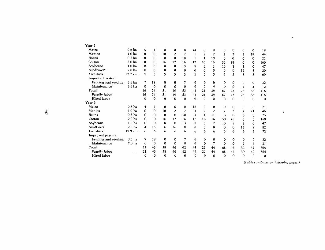
Year 2Maize 0.5 ha 4 1 0 0 0 14 0 0 0 0 0 0 19Manioc 1.0 ha 0 0 10 2 2 1 2 2 2 2 2 19 44Beans 0.5 ha 0 0 0 0 10 1 1 10 0 0 0 0 22Cotton 2.0 ha 0 0 16 12 16 12 10 16 50 28 0 0 160Soybeans 1.0 ha 0 0 0 0 13 8 3 2 10 8 3 0 47Sunflower' 2.0 ha 0 0 0 0 0 0 0 0 0 0 12 8 20Livestock 17.2 a.u. 5 5 5 5 5 5 5 5 5 5 5 5 60Improved pasture
Fencing and seeding 3.5 ha 7 18 0 0 7 0 0 0 0 0 0 0 32Maintenanced 3.5 ha 0 0 0 0 0 0 0 4 0 0 4 4 12
Total 16 24 31 19 53 41 21 39 67 43 26 36 416Family labor 16 24 31 19 53 41 21 39 67 43 26 36 416Hired labor 0 0 0 0 0 0 0 0 0 0 0 0 0
Year 3Maize 0.5 ha 4 1 0 0 0 16 0 0 0 0 0 0 21Manioc 1.0 ha 0 0 10 2 2 1 2 2 2 2 2 21 46Beans 0.5 ha 0 0 0 0 10 1 1 11 0 0 0 0 23Cotton 2.0 ha 0 0 16 12 16 12 10 16 50 28 0 0 160Soybeans 1.0 ha 0 0 0 0 13 8 3 2 10 8 3 0 47Sunflower 2.0 ha 4 18 6 26 8 0 0 0 0 0 12 8 82Livestock 19.9 a.u. 6 6 6 6 6 6 6 6 6 6 6 6 72Improved pasture
Fencing and seeding 3.5 ha 7 18 0 0 7 0 0 0 0 0 0 0 32Maintenance 7.0 ha 0 0 0 0 0 0 0 7 0 0 7 7 21
Total 21 43 38 46 62 44 22 44 68 44 30 42 504Family labor 21 43 38 46 62 44 22 44 68 44 30 42 504Hired labor 0 0 0 0 0 0 0 0 0 0 0 0 0
(Table continues on following pages.)

Table 4-7 (continued)
Year and cropor activity Unit Jul Aug Sept Oct Nov Dec Jan Feb Mar Apr May Jun Total
Year 4Maize 0.5 ha 4 1 0 0 0 16 0 0 0 0 0 0 21Manioc 0.5 ha 0 0 5 1 1 0 1 1 1 1 1 10 22Beans 0.5 ha 0 0 0 0 10 1 1 11 0 0 0 0 23Cotton 2.2 ha 0 0 18 13 18 13 11 18 59 33 0 0 183Soybeans 2.2 ha 0 0 0 0 29 18 7 4 22 22 7 0 109Sunflower 2.2 ha 4 18 6 28 8 0 0 0 0 0 13 9 86Livestock 22.7 a.u. 7 7 7 7 7 7 7 7 7 7 7 7 84Improved pasture
Maintenance 10.5 ha 0 0 0 0 0 0 0 10 0 0 10 10 30Total 15 26 36 49 73 55 27 51 89 63 38 36 558
Family labor 15 26 36 49 70 55 27 51 70 63 38 36 536Hired labor 0 0 0 0 3 0 0 0 19 0 0 0 22
Year 5Maize 0.5 ha 4 1 0 0 0 16 0 0 0 0 0 0 21Manioc 0.5 ha 0 0 5 1 1 0 1 1 1 1 1 12 24Beans 0.5 ha 0 0 0 0 10 1 1 11 0 0 0 0 23Cotton 2.5 ha 0 0 20 15 20 15 12 20 68 38 0 0 208Soybeans 2.5 ha 0 0 0 0 32 20 8 5 25 25 8 0 123Sunflower 2.5 ha 4 20 7 31 9 0 0 0 0 0 15 10 96Livestock 24.6 a.u. 8 8 8 8 8 8 8 8 8 8 8 8 96Improved pasture
Maintenance 10.5 ha 0 0 0 0 0 0 0 10 0 0 10 10 30Total 16 29 40 55 80 60 30 55 102 72 42 40 621
Family labor 16 29 40 55 70 60 30 55 70 70 42 40 577Hired labor 0 0 0 0 10 0 0 0 32 2 0 0 44

Year 6Maize 0.5 ha 4 1 0 0 0 16 0 0 0 0 0 0 21Manioc 0.5 ha 0 0 5 1 1 0 1 1 1 1 1 12 24Cotton 3.0 ha 0 0 24 18 24 18 15 27 84 48 0 0 258Soybeans 3.0 ha 0 0 0 0 39 24 9 6 33 33 12 0 156Sunflower 3.0 ha 5 22 8 38 12 0 0 0 0 0 18 12 115Livestock 25.1 a.u. 8 8 8 8 8 8 8 8 8 8 8 8 96Improved pasture
Maintenance 10.5 ha 0 0 0 0 0 0 0 10 0 0 10 10 30Total 17 31 45 65 84 66 33 52 126 90 49 42 700
Family labor 17 31 45 65 70 66 33 52 70 70 49 42 610Hired labor 0 0 0 0 14 0 0 0 56 20 0 0 90
Years 7-20Maize 0.5 ha 4 1 0 0 0 18 0 0 0 0 0 0 23Manioc 0.5 ha 0 0 5 1 1 0 1 1 1 1 1 12 24Cotton 3.0 ha 0 0 24 18 24 18 15 27 84 48 0 0 258Soybeans 3.0 ha 0 0 0 0 39 24 9 6 33 33 12 0 156Sunflower 3.0 ha 6 27 9 45 15 0 0 0 0 0 18 12 132Livestock 25.0 a.u. 8 8 8 8 8 8 8 8 8 8 8 8 96Improved pasture
Maintenance 10.5 ha 0 0 0 0 0 0 0 10 0 0 10 10 30Total 18 36 46 72 87 68 33 52 126 90 49 42 719
Family labor 18 36 46 70 70 68 33 52 70 70 49 42 624Hired labor 0 0 0 2 17 0 0 0 56 20 0 0 95
ha Hectares; a.u. animal units. b. Assumes 70 work days per month of available family labor.Source: Calculated from tables 4-4 and 4-6. c. Area and labor requirement for sunflower apply to the year of planting.a. Assumes five minutes a day per animal unit, eight hours a day, and thirty Thus, the area assumed in the first five months of project year 5 is the 2.2
days a month. The labor requirement is based on the animal units at the hectares planted in May of project year 4.beginning of the year (as given in table 4-11) divided by 100 to give the labor d. Calculated on the basis of improved pasture established in previousrequirement for a single farm. See text (the subsection "Farm production. years (as shown in table 4-4). Thus, in year 2 it is based on 3.5 hectares and inLivestock") for a discussion of this convention. year 3 on 7.0 hectares.

110 FINANCIAL ASPECTS OF PROJECT ANALYSIS
Some analysts like to work out a labor use diagram such as the oneshown in figure 4-3. This usually is done only for the full-developmentsituation. The graphic presentation makes the problem of peak laborrequirements readily apparent.
Once the total hired labor has been determined, it must be allocatedamong the various crops so that it may be included in the proper categoryof operating expenditure. This is done in table 4-8. In the Paraguayexample the allocation is made in proportion to the total work days
Figure 4-3. Labor Use Diagram for Project Years 7-20,20-Hectare Mixed Farm, Paraguay Project
130
120-
110
100
90
80 - Family Xlabor
70 - - '- - - - - - - - -
60-
50-
40-
30-
20-
loll1 jl
Jul Aug Sept Oct Nov Dec Jan Feb Mar Apr May Jun
MonthCrop TotalEI Cotton O 0 24 18 24 18 15 27 84 48 0 0 258EC Soybeans 0 0 O 0 39 24 9 6 33 33 12 0 156E Sunllower 6 27 9 45 15 0 0 0 0 0 18 12 1321U Maize 4 1 0 0 0 18 0 0 0 0 0 0 237 Manioc 0 0 5 1 1 0 1 1 1 1 1 12 24E Improved pasture
maintenance 0 0 0 0 0 0 0 10 0 0 10 10 30M Livestock 8 8 8 8 8 8 8 8 8 8 8 96
Total 18 36 46 72 87 68 33 52 126 90 49 42 719Family labor 18 36 46 70 70 68 33 52 70 70 49 42 624Hired labor 0 0 0 2 17 0 0 0 56 20 0 0 95
Source: Table 4-7.

FARM INVESTMENT ANALYSIS ill
required for each cash crop in each month for which hired labor would beneeded. In other circumstances, such a mechanistic allocation would beinappropriate. In many areas, certain crop operations are done by hiredlabor and not by family labor, even if family labor is available. Thus, inSoutheast Asia, transplanting rice is done in many areas entirely by hiredlabor; the only family labor engaged is that of the farmer himself, whosupervises the work. Both the amount of hired labor and its allocationamong crops should be closely related to the expected cultural practicesof people in the project area.
Farm production
Having determined the use of land and labor resources for the patternfarm, the analyst next assesses the projected farm production. The in-vestment analysis of crop and pasture and livestock production is dis-cussed in this subsection, and issues of valuation (both of farm produc-tion and incremental residual value on the farm) are addressed.
Table 4-8. Hired Labor by Crop and Month,20-Hectare Mixed Farm, Paraguay Project(work days)
Year andcropa Jul Aug Sept Oct Nov Dec Jan Feb Mar Apr May Jun Total
Year 4Cotton 0 0 0 0 1 0 0 0 14 0 0 0 15Soybeans 0 0 0 0 2 0 0 0 5 0 0 0 7
Total 0 0 0 0 3 0 0 0 19 0 0 0 22Year 5
Cotton 0 0 0 0 3 0 0 0 23 1 0 0 27Soybeans 0 0 0 0 5 0 0 0 9 1 0 0 15Sunflower 0 0 0 0 1 0 0 0 0 0 0 0 1
Total 0 0 0 0 gb 0 0 0 32 2 0 0 43b
Year 6Cotton 0 0 0 0 4 0 0 0 40 12 0 0 56Soybeans 0 0 0 0 7 0 0 0 16 8 0 0 31Sunflower 0 0 0 0 2 0 0 0 0 0 0 0 2
Total 0 0 0 0 1 3 b 0 0 0 56 20 0 0 8 9b
Years 7-20Cotton 0 0 0 1 5 0 0 0 40 12 0 0 58Soybeans 0 0 0 0 8 0 0 0 16 8 0 0 32Sunflower 0 0 0 1 3 0 0 0 0 0 0 0 4
Total 0 0 0 2 1 6 b 0 0 0 56 20 0 0 9 4 b
Source: Calculated from table 4-7.a. Hired labor is allocated to cash crops-cotton, soybeans, and sunflower-in propor-
tion to their total labor requirements in that month. In November of year 4, for example, 55work days are required for cash crops, of which 3 work days are to be hired. Eighteen workdays are required for cotton. To determine the hired labor for cotton, the proportion of totallabor required for cash crops that is to be applied to cotton is multiplied by the total hiredlabor requirement for the month; this gives the hired labor to be applied to cotton, or I workday {[18 . (18 + 29 + 8)] x 3 = I}.
b. Does not equal the total in table 4-7 because of rounding.

112 FINANCIAL ASPECTS OF PROJECT ANALYSIS
CROPS AND PASTURE. For crops and pasture, the yield and carryingcapacity are tabulated as illustrated in table 4-9. In the table, yields areshown only for crops and pasture actually in the cropping pattern in theyear reported. Thus, no without-project yield is reported for soybeans,whereas for sunflower, which will be planted following cotton in year 2,yield is reported only beginning in year 3 since the first crop is notharvested until that time.
Multiplying the production per hectare by the number of hectares ofeach of the crops and of pasture in the land use pattern shown in table 4-4,we obtain the crop and pasture production illustrated in table 4-10.Again, since sunflower is first planted in year 2 but first harvested in year3, the production from the first planting of 1.8 tons is shown in year 3.Similarly, sunflower planted each year produces in the following year.
Because all the feed for the livestock to be produced on the patternfarm in the Paraguay project is assumed to come from pasture, nodeduction is made in table 4-10 for crops to be used for feed. Should theproduction pattern of a model farm call for the use of crops and cropby-products for feed, table 4-10 would then be adjusted to show that use.Total production of crops would be shown and expanded to include cropby-products if these were to be fed or if they have a sale value. From thistotal would be deducted the feed consumption taken from an estimate offeed requirement and production such as that illustrated in table 4-30.The result would be the net production available for sale or householdconsumption.
LIVESTOCK. Herd composition, purchases, and sales are given in table4-1 1. Projecting the herd (or flock) composition, purchases, and sales in afarm investment analysis that involves livestock introduces a computa-tional process that can become quite complex.
Table 4-9. Yield and Carrying Capacity,20-Hectare Mixed Farm, Paraguay Project
With projectWithout
Product project Year 1 2 3 4 5 6 7-20
Crops(tons per hectare)
Maize 1.1 1.1 1.1 1.2 1.2 1.3 1 3 1.4
Manioc 18.0 18.0 18.0 20.0 20.0 22.0 22.0 24.0
Beans 0.9 0.9 0.9 1.0 1.0 1.0 - -
Cotton 1.3 1.3 1.5 1.5 1.6 1.6 1.7 1.7
Soybeans - - 1.4 1.4 1.6 1.6 1.8 1.8
Sunflower - - - 0.9 1.0 1.1 1.2 1.2
Pasture(animal units per hectare)
Natural 1.2 1.2 1.2 1.2 1.2 1.2 1.2 1.2
Improved - 2.5 2.5 2.5 2.5 2.5 2.5 2.5
Source: Same as table 4-4.

FARM INVESTMENT ANALYSIS 113
Table 4-10. Crop and Pasture Production,20-Hectare Mixed Farm, Paraguay Project(tons)
With projectWithout
Product project Year 1 2 3 4 5 6 7-20
CropsTotal production
Maize 0.6 0.6 0.6 0.6 0.6 0.6 0.6 0.7Manioc 18.0 18.0 18.0 20.0 10.0 11.0 11.0 12.0Beans 0.4 0.4 0.4 0.5 0.5 0.5 - -Cotton 2.6 2.6 3.0 3.0 3.5 4.0 5.1 5.1Soybeans - - 1.4 1.4 3.5 4.0 5.4 5.4Sunflowera - - - 1.8 2.0 2.4 3.0 3.6
Feed consumption bMaize - - - - - - - -Manioc - - - - - - - -Soybeans - - - - - - - -Sunflower - - - - - - - -
Net productionavailable forsale or house-hold consumption
Maize 0.6 0.6 0.6 0.6 0.6 0.6 0.6 0.7Manioc 18.0 18.0 18.0 20.0 10.0 11.0 11.0 12.0Beans 0.4 0.4 0.4 0.5 0.5 0.5 - -
Cotton 2.6 2.6 3.0 3.0 3.5 4.0 5.1 5.1Soybeans - - 1.4 1.4 3.5 4.0 5.4 5.4Sunflower - - - 1.8 2.0 2.4 3.0 3.6
PastureCarrying capacity
(animal units) 12.6 17.2 21.7 26.2 26.2 26.2 26.2 26.2
Source: Calculated from tables 4-4 and 4-9.a. Sunflower is harvested in the year following planting. Thus, the production in year 2 is
zero, and in year 3 it is 1.8 tons, which is determined by multiplying the 2.0 hectares plantedin year 2 by the yield of 0.9 tons per hectare harvested in year 3 (2.0 x 0.9 = 1.8).
b. If there were a substantial livestock production activity on the farm that used crops forfeed, the amounts would be estimated in a feed requirement and production table such astable 4-30 and tabulated here. The table would be expanded to include crop by-productsused for feed. As indicated, the use of crops for feed would be deducted from the totalproduction, and the result would be the net production available for sale or householdconsumption.
Herd projections are done to forecast use of future facilities, pasture, orfeed by applying technical coefficients, such as those shown at the bottomof table 4-1 1, to trace the changes in the size and composition of the herd.
For poultry, stall feeding, or feedlot projections, it is usually assumedthat enough young animals can be purchased in a given year to bring thenumbers up to the level of feed availability or of proposed productionfacilities. Brown (1979, pp. 76-85) gives a methodology for broiler andegg production. For pigs, a projection is made applying the technicalcoefficients; since the gestation period of swine is short, the projection issimplified and uncomplicated.

114 FINANCIAL ASPECTS OF PROJECT ANALYSIS
Table 4-11. Herd Composition, Purchases, and Sales,100 20-Hectare Mixed Farms, Paraguay Project(head)
With projectWithout
Item project Year 1 2 3 4 5 6 7-20
Herd composition at beginning of yearBulls 100 100 100 100 100 100 100 100Breeding cows 500 500 655 800 800 800 800 800Heifers 1-2 years 157 157 157 221 294 285 285 285Heifers 2-3 years 152 152 152 152 217 288 279 279Steers 1-2 years 157 157 157 221 294 285 285 285Steers 2-3 years 152 152 152 152 217 288 279 279Steers 3-4 years 147 147 147 147 149 213 282 273Work oxen - 0 200 200 200 200 200 200Total 1,365 1,365 1,720 1,993 2,271 2,459 2,510 2,501
Animal units 1,365 1,365 1,720 1,993 2,271 2,459 2,510 2,501Carrying capacity
(beginning of year)a 1,260 1,260 1,720 2,170 2,620 2,620 2,620 2,620
PurchasesBulls 18 33 20 20 20 20 20 20Heifers 2-3 years 0 91 131 2 0 0 0 0Steers 1-2 years 0 0 0 0 0 0 0 0Work oxen 0 200 38 36 36 36 36 36Total 18 324 189 58 56 56 56 56
Sales (including culls)Culled bulls 15 30 17 18 18 18 18 18Culled cows 60 60 98 120 112 112 112 112Culled heifers 8 8 15 15 22 29 28 28Surplus heifers 2-3 years 64 0 0 0 63 125 117 117Steers 1-2 years 0 0 0 0 0 0 0 0Steers 3-4 years 143 143 143 144 146 209 276 268Culled work oxen - 0 32 32 32 32 32 32Total 290 241 305 329 393 525 583 575
Herd productivity(percent)b 20 23
Technical coefficients (percent)Calving rate 70 70 75' 80' 75 75 75 75Calf mortality 10 10 10 8 5 5 5 5Adult mortality 3 3 3 2 2 2 2 2Culling rate (bulls) 15 30 17 18 18 18 18 18Culling rate (cows) 12 12 15 15 14 14 14 14Culling rate (heifers) 5 5 10 10 10 10 10 10Culling rate (work oxen) - 0 16 16 16 16 16 16Bulls/breeding femalesd -
Carrying capacity(per hectare; end of year)a 1.2 1.6 2.1 2.5 2.5 2.5 2.5 2.5
Source: Same as table 4-4 (annex 1, table 18). See computations in table 4-27.a. In animal units. The carrying capacity at the beginning of the year is determined by
multiplying the animal units per farm at the end of the previous year (given in table 4-10) bythe 100 farms in the model. The carrying capacity per hectare at the end of the year isdetermined by dividing the animal units per farm by the 10.5 hectares of pasture on eachfarm; it is thus a weighted average of natural and improved pasture.
(Notes continue on the following page.)

FARM INVESTMENT ANALYSIS 115
The projection can become computationally quite complicated,however, for larger animals fed mainly pasture, such as sheep or cattleused for dairy or beef production. The project analyst often relies on thelivestock technician for these projections and simply incorporates theminto his farm investment analysis. But livestock technicians themselvesmay be unfamiliar with the details of how to make these computations-and especially with how to make them so they conform to the accountingconvention adopted here for the farm investment analysis. For thisreason, the computation for the herd projection in the Paraguay exampleis discussed in considerable detail in the appendix to this chapter (wheredefinitions of the specialized livestock terms may also be found). Thismethodology can be adapted, with only minor variations, to projectionsfor dairy animals. As in the treatment here, the details of the projectionneed not form part of the main body of most project reports; only asummary need be given (as in table 4-11 from the Paraguay example),with the details laid out in an annex or in the project file.
Projecting the herd composition on a small farm when larger animalsare to be produced introduces the difficult problems of divisibility. Asnoted, herd projections for animals that are mainly grazed on pasture arebased on the estimated feed availability. Technical coefficients, such asmortality and calving rates, are often directly influenced by the amountof available feed, but in cattle production changes do not happen im-mediately. For example, an increase in feed availability in one seasonwill improve the calving rate and decrease calf losses only during thenext season.
The projected coefficients are applied to the herd at the beginning ofthe project. The result begins to appear in the herd composition at thebeginning of year 2. Often, the projected coefficients indicate that theherd's composition and its overall size will not change fast enough toutilize the increased feed available. As a solution, in-calf heifers can bepurchased to increase the reproductive component of the herd, or feedersteers can be purchased for fattening until the herd can utilize the forageresources.
This use of technical coefficients raises few problems of interpretationfor larger farms or ranches with herds of 100 or more animals. For smallfarms, however, the technical coefficients lead to many "fractional ani-mals." In the Paraguay example, for instance, at full development fromyears 7 through 20 the farm is expected to have eight breeding cows. Theadult mortality is expected to be 2 percent, so do we report that 0.16 cowsdie each year (8 x 0.02 = 0.16)? Such nonsensical results have led project
b. Herd productivity is the sum of the off-take rate and the herd growth rate. Only thevalues for a stable herd are given.
c. Represents a weighted average between the calving rate of breeding cows in theexisting herd, which is 70 percent, and that of purchased in-calf heifers, which is nearly 100percent.
d. Note that in this project a minimum of one bull per farm is assumed, or a minimum of100 bulls on 100 farms. Normally the number of bulls per 100 breeding females would bethree or four for all years.

116 FINANCIAL ASPECTS OF PROJECT ANALYSIS
analysts to seek means to overcome the divisibility problem. Some havesimply ignored technical coefficients, such as mortality, that result invery small, fractional animal figures. This omission, however, consider-ably distorts the pattern farm investment analysis. To avoid such distor-tion, other analysts have devised systems that carry fractional animals inthe computation until the fractions add up to a whole animal, which isthen reported. In the Paraguay example, for instance, the calving rate atfull development is 75 percent. Thus, six calves are born, of which halfmay be expected to be female. Calf mortality is 5 percent, and this gives afigure of 2.8 to be carried over to the next year as heifers 1-2 years old[8 x 0.75 . 2 - (8 x 0.75 - 2 x 0.05) = 2.8]. Of these, 2 percent arereported and 0.8 is carried over to the following year, which then willshow a figure of 3.6 (0.8 + 2.8 = 3.6). Of these, 3 are reported and 0.6 iscarried forward, and so forth.
Mortality may sometimes be treated by incorporating a more formalprobability assumption. Such systems become quite complex and in theend do not satisfactorily project an individual small herd. Anotherapproach that is increasingly used-and that is adopted and recom-mended here-is to do the herd projection for a number of farms, say 100,that will contain or eliminate the divisibility problem. Purchases andsales are then valued, and only the values are entered in the farm invest-ment analysis for a single pattern farm. In effect, this says that on theaverage a farm will have a certain level of purchases and sales. This, too,is not a fully satisfactory convention. Its results do not state, for example,how many animals are actually on the farm at any given time. It doeshave the virtue, however, of being simpler than other systems-even if itis still quite complex-and of generating somewhat less distortion.
Project designers may want to introduce an insurance scheme to pro-tect project participants from, say, the loss of a bull. Then, in effect, thevalues in the farm investment analysis for a single farm for the purchaseof bulls include an insurance premium that insures that the farmer willbe reimbursed in the event of the death of a bull. Such insurance schemesare found in developing countries, but they give rise to possibilities ofabuse and to difficult administrative problems, and they often are notvery effective.
In the Paraguay example summarized in table 4-11, the herd composi-tion is given for each major class of animals without the project and foreach project year. (The table is drawn from the worksheet reproduced intable 4-27.) Note that the analyst assumed that each farm would have abull, so that the number of bulls remains 100, many more than would beneeded if the analysis were, indeed, for a single herd rather than for 100small farms. Note, also, the purchase of draft animals at the end of thefirst year. It is assumed that each farm will purchase two work oxen. Thetotal animal units for the herd are shown, and for convenience this figureis compared with the carrying capacity. As noted in the appendix to thischapter, the number of breeding cows has been rounded to an evenmultiple of the number of farms in the model so that each farm has fivebreeding cows without the project and increases its herd to eight breed-

FARM INVESTMENT ANALYSIS 117
ing cows at full development. As a result, the total of animal units doesnot very closely approximate the carrying capacity. Since estimates ofcarrying capacity are quite approximate, however, overstocking of up to10 percent would probably be acceptable.
Purchases of each class of animal are treated next in the investmentanalysis; these will form the basis for the investment and operatingexpenditure for the livestock aspect of the 20-hectare mixed farm. Thesales give the basis for the inflow for the farm. The herd productivity, ameasure of the efficiency of the herd, is also given; it relates the numberof head sold plus the increase in herd size to the number of head carriedat the beginning of the year. Only the figures for the stable herd withoutthe project and at full development are given. The dynamics of herdgrowth tend to distort the measure during the period when the herd isincreasing in size. (The details of the computation are given in table4-28.) Finally, the technical coefficients for the herd are given. These arecrucial parameters of the herd growth and are indicators of managementeffectiveness, animal health care, and feed availability.
When feed concentrates are important in the farm production pattern,it may be desirable to project the feed requirements the livestock activitywill involve. (An illustrative example is included in tables 4-29 and 4-30in the appendix to this chapter in connection with the discussion of herdprojections.)
In some instances it may be desirable to report yield per animal if thevaluation system is based, say, on kilograms. In the Paraguay examplethe prices are based on individual animals without regard to weight, soyield per animal is not needed and is therefore not illustrated.
VALUATION. To begin the valuation of the farm production, the farm-gate prices for items entering the farm investment analysis are listed asshown in table 4-12. (The symbol for Paraguayan guaranis is G.) If afarm-gate price is used in only one table of the investment analysis, itmay not be included in the farm-gate price table but may appear in theappropriate table. (Such is the case, for example, of the prices for landimprovement, which are included in table 4-15, devoted to investment,and not in the table of farm-gate prices.) Some farm-gate prices werecollected and projected by the project analyst on the basis of fieldobservation. Other prices were collected in the field but forecast usingthe projections of the World Bank. Prices and their derivation werediscussed in more detail in chapter 3.
The value of production for the farm is given in table 4-13. For crops,values are determined by multiplying the production in table 4-10 by theprice per ton in table 4-12. For livestock, the value is obtained by multi-plying sales from table 4-11 by the price per animal given in table 4-12.The product is then divided by 100 to give the value for a single farm, inline with the convention recommended to avoid the divisibility problem.
INCREMENTAL RESIDUAL VALUE. In the last year of the farm investmentanalysis, the incremental residual (or terminal) value on the farm is

118 FINANCIAL ASPECTS OF PROJECT ANALYSIS
Table 4-12. Farm-Gate Prices, 20-Hectare Mixed Farm,Paraguay Project(thousands of i)
Project year
Itema 1 2 3-5 6-20
Farm labor (per work day) 0.3 0.3 0.3 0.3Crops (per ton)
Maize 12.0 12.0 12.0 12.0Manioc 3.0 3.0 3.0 3.0Beans 28.0 28.0 28.0 28.0Cotton 44.4 45.1 45.1 44.9Soybeans 23.6 20.9 26.2 28.9Sunflower 20.0 20.0 20.0 20.0
Livestock (per head)Bulls 30.0 30.0 32.4 33.6Culled bulls 23.0 23.0 24.8 25.8Breeding cows 18.7 18.7 20.2 20.9Culled cows 17.0 17.0 18.4 19.0Heifers 1-2 years 12.5 12.5 13.5 14.0Heifers 2-3 years 18.7 18.7 20.2 20.9Culled heifers 2-3 years 17.0 17.0 18.4 19.0Steers 1-2 years 12.5 12.5 13.5 14.0Steers 2-3 years 18.7 18.7 20.2 20.9Steers 3-4 years 23.0 23.0 24.8 25.8Work oxen 35.0 35.0 37.8 39.2Culled work oxen 23.0 23.0 24.8 25.8
; Paraguayan guaranis.Source: Same as table 4-4.a. Prices of maize, soybeans, and livestock are adjusted for the real price changes
projected by the Commodities and Export Projections division of the World Bank. Otherprices are assumed to remain constant in real terms.
included among the inflows in the farm budget and "credited" to theproject investment. This is done because not all the utility of an invest-ment may be exhausted in the course of a project. Note that it is theincremental value that is sought, not the total value. In some instancesthere is no distinction, since the value of an item such as constructionmay be entirely incremental. But for items such as land, livestock, andworking capital, there may have been values existing at the beginning ofthe project, and only the incremental residual value may properly becredited to the project investment. Since the incremental residual valueenters the farm investment analysis in the final year, it bears relativelylittle weight in the discounting process. As a result, rather broad esti-mates of residual values are acceptable in project analysis.
Three kinds of residual value may be noted. The first is the salvagevalue of capital assets that have been largely consumed by the end of theproject and that, for the most part, can only be salvaged for their scrapvalue or have only a short portion of their normal life expectancy remain-ing at the end of the project period. Buildings and other construction ormachinery such as irrigation pumps or tractors are common examples. Asecond kind of residual value is the working capital. This is automati-

FARM INVESTMENT ANALYSIS 119
cally allowed for under the accounting convention we have adopted forthe farm investment analysis. The third kind of residual value is the valueof items that have a substantial useful life remaining at the end of theproject and may even have increased in value as a result of the projectinvestment; land with associated improvements and a livestock herd areexamples.
All three kinds of residual value are illustrated for the Paraguay exam-ple in table 4-14. In a land improvement project such as this one, thereusually would be an entry for the incremental value of land, although inthis instance the analyst chose not to include it because the site inParaguay is a frontier area and the land market is not very active. In morecrowded societies where a project involves land improvement such asbetter irrigation and drainage, the incremental value of the land mightbe quite substantial. Next for consideration would be the incrementalresidual value of construction. In the Paraguay example, the constructionis all incremental, so the incremental residual value is quite simplyobtained by taking a proportion of the initial construction, in this case 10percent. The incremental residual value of equipment is assumed to benegligible, although that would not necessarily be the case in otherprojects. Then the analyst considers the incremental value of livestock. Inthis case, care must be taken to distinguish between the total residualvalue of the livestock herd and the incremental residual value. Therewas, of course, a livestock herd at the beginning of the project, so only theincreased value of the herd at the end of the project can be attributed tothe project investment itself. Hence, each class of animals is valued at thebeginning of the project and at the end of the project, and only thedifference-or increment-is carried forward as the incremental re-sidual value. Finally, there is the total incremental working capital. Thereader will recall that, in the discussion of the accounting convention forfarm investment analysis, considerable attention was devoted to esti-mating the incremental working capital year by year. Once this is done,all that is needed to obtain the total incremental working capital issimply to add the incremental working capital for each year algebra-ically-that is, adding the increases and subtracting decreases-toobtain the incremental residual value entered in the final year.
Farn inputs
When the estimates of production are complete, the estimates of thenecessary inputs may be prepared. Inputs comprise the investment,operating expenditure, and incremental working capital for the project.
INVESTMENT. Investment for the project is a crucial element. The in-vestment contemplated for the Paraguay pattern farm is given in table4-15. It is convenient to show the unit and unit cost in the investmenttable; for convenience, items appearing only in the investment table maybe omitted from the farm-gate price table. As in this presentation, thetotal physical investment may be incorporated in the investment cost

Table 4-13. Value of Production, 20-Hectare Mixed Farm, Paraguay Project(thousands of ;)
Without project With project
Item Year 1 2 3-5 6-20 1 2 3 4 5 6 7-20
Crops'Maize 7.2 7.2 7.2 7.2 7.2 7.2 7.2 7.2 7.2 7.2 8.4Manioc 54.0 54.0 54.0 54.0 54.0 54.0 60.0 30.0 33.0 33.0 36.0Beans 11.2 11.2 11.2 11.2 11.2 11.2 14.0 14.0 14.0 - -Cotton 115.4 117.3 117.3 116.7 115.4 135.3 135.3 157.8 180.4 229.0 229.0Soybeans - - - - - 29.3 36.7 91.7 104.8 156.1 156.1Sunflower - - - - - - 36.0 40.0 48.0 60.0 72.0
Total 187.8 189.7 189.7 189.1 187.8 237.0 289.2 340 7 387.4 485.3 501.5
LivestockbCulled bulls 3.4 3.4 3.7 3 9 6.9 3.9 4.5 4.5 4.5 4.6 4.6Culled cows 10.2 10.2 11.0 11.4 10.2 16.7 22.1 20.6 20.6 21.3 21.3Culled heifers 1.4 1.4 1.5 1.5 1.4 2.6 2.8 4.0 5.3 5.3 5.3Surplus heifers 12.0 12.0 12.9 13.4 0 0 0 12.7 25.2 24.5 24.5Steers 3-4 years 32.9 32.9 35.5 36.9 32.9 32.9 35.7 36.2 51.8 71.2 69.1Culled work oxen - - - - - 7.4 7.9 7.9 7.9 8.3 8.3
Total 59.9 59.9 64.6 67.1 51.4 63.5 73.0 85.9 115.3 135.2 133.1
Total value 247 7 249.6 254.3 256.2 239.2 300.5 362.2 426 6 502.7 620.5 634.6
Source: Calculated from tables 4-10, 4-11, and 4-12. b. Sales from table 4-11 multiplied by the price per animal from table 4-12;a. Production from table 4-10 multiplied by the price per ton from table product is then divided by 100 to give the value for a single farm. See text for a
4-12. For year 2 without the project, for example, the value of cotton is the discussion of this convention.without-project production from table 4-10 times the price in year 2 in table4-12.

FARM INVESTMENT ANALYSIS 121
Table 4-14. Incremental Residual Value,20-Hectare Mixed Farm, Paraguay Project(thousands of 0)
Value
At beginning At end Incre-Item of project of project mental
Land a a a
Constructionb 0 18.0 18.0Equipmentc 0 0 0Livestockd
Bulls 30.0 33.6Breeding cows 93.5 167.2Heifers 1-2 years 19.6 39.9Heifers 2-3 years 28.4 58.3Steers 1-2 years 19.6 39.9Steers 2-3 years 28.4 58.3Steers 3-4 years 33.8 70.4Work oxen - 78.4Total 253.3 546.0 292.7
Working capitale - - 119.9Total 430.6
Source: Calculated from other tables as noted.a. In the Paraguay example, the analyst chose not to include an incremental value of land
improvements in his computation of residual value. This amount usually is included ifthere has been substantial land improvement.
b. The residual value of construction is taken as 10 percent of the total constructioninvestment given in table 4-15.
c. The residual value of equipment is assumed to be negligible. Only equipment pur-chased for the project is included in the computation, not the equipment existing on thefarm at the beginning of the project.
d. The value of the livestock at the beginning of the project is calculated from the herdcomposition at the beginning of the year in table 4-11 multiplied by the year-I prices intable 4-12. The value of the livestock at the end of the project is calculated from the year-20herd composition in table 4-11 multiplied by the year-20 prices in table 4-12.
e. From table 4-17.
table; in other instances, a separate table may be needed. Although it isnot shown for the Paraguay example, including the foreign exchangecomponent of the investment cost is often desirable. It is important thatan agricultural project report detail the foreign exchange needed for theproject because the availability of foreign exchange may be a majorconstraint.
Investment for the Paraguay example is divided into land improvement,construction, equipment, and livestock, the major categories likely to befound in an agricultural project. Within each category the major itemsare noted, and the investment for them is tabulated by project year. Thetotal investment by year and for the pattern as a whole is given. Note howthe analyst accommodated the existing equipment found on projectfarms in this pattern by listing equipment totaling 0206 thousand, butthen subtracting ;50 thousand as an average of existing equipment.
For livestock, it is assumed that all heifer purchases and culling inexcess of that normally done without the project are an investment.

122 FINANCIAL ASPECTS OF PROJECT ANALYSIS
Table 4-15. Investment, 20-Hectare Mixed Farm, Paraguay Project(thousands of ;)
Project yearUnit
Itema cost 1 2 3 Total
Land improvement (per hectare)Clear, cut and burn
forestb 15.0 52.5 52.5 52.5 157.5Destumpingc 20.0 100.0 0 40.0 140.0Pasture
establishmentd 1.0 3.5 3.5 3.5 10.5Total 156.0 56.0 96.0 308.0
Construction (per single unit)Storage 40.0 40.0 0 0 40.0Welle 50.0 50.0 0 0 50.0Fencing wire (for 1 ha) 8.6 30.1 30.1 30.1 90.3Total 120.1 30.1 30.1 180.3
Equipment (per single unit)Plow 18.0 18.0 0 0 18.0Disc harrow 65.0 65.0 0 0 65.0Seeder 30.0 30.0 0 0 30.0Cultivator 17.0 17.0 0 0 17.0Ox cart 50.0 50.0 0 0 50.0Sprayer 11.0 11.0 0 0 11.0Hand tools 15.0 15.0 0 0 15.0Subtotal 206.0 0 0 206.0Less existing
equipmentf ( 50.0) 0 0 ( 50.0)Total 156.0 0 0 156.0
Livestock (per head)9Heifers 2-3 yearsh - 17.0 24.5 0.4 41.9Bulls' 30.0 4.5 0 0 4.5Work oxenJ 35.0 70.0 0 0 70.0Total 91.5 24.5 0.4 116.4
Total investment 523.6 110.6 126.5 760.7
Note: Parentheses indicate negative numbers.Source: Same as table 4-4 (annex 1, table 16).a. Family labor is valued at its opportunity cost (see the discussion of the farm budget).
The number of work days required is given in table 4-7.b. Clearing is done by a contractor. It is assumed that forest will be cleared to establish
improved pasture and that clearing proceeds at the pace given for incremental improvedpasture in table 4-4.
c Destumping is done by a contractor. Following the land use given in table 4-4, it isassumed that 5 hectares, consisting of the 4 hectares of existing cropland plus the addi-tional hectare to be cultivated in year 2, will be destumped in year 1 and the remaining 2hectares in year 3.
d. The cost of pasture establishment includes only the purchase of colonial variety grass(Panicum maximum).
e. An open well of 20 meters at q;2.5 thousand a meter.f. It is assumed that, of the equipment listed, farmers will already own items of a total
value amounting to (50 thousand (in parentheses)g. From the purchases in table 4-11 multiplied by the prices in table 4-12, the product
then divided by 100 to give the value for a single farm. See text for a discussion of thisconvention. Normal replacement of death loss and culls is considered an operating cost.
h. All heifer purchases are considered investment. The prices are taken from table 4-12.i. The excess over normal death loss and without-project culling for bulls in year I is
considered investment. For the 100-farm herd, table 4-27 shows 33 replacement bulls will

FARM INVESTMENT ANALYSIS 123
Thus, the heifers purchased are included in the investment tabulation, asare the excess bulls culled in year 1. The work oxen purchased in year 1are clearly an investment. In years 2 through 20, oxen purchased are toreplace animals lost through death and culling; thus, these purchases areconsidered as operating expenditure. The amounts for the livestock in-vestment are obtained by taking the numbers of animals given in table4-11, multiplying by the prices in table 4-12, and then dividing by 100 toobtain the amount from a single farm. This is in line with the conventionrecommended in the discussion of the herd composition, purchases, andsales. (The sale of replaced livestock, such as indigenous cows sold be-cause improved cows are purchased, is better treated as a "negativeinvestment" and not as a benefit.)
In the investment cost tabulation, allowance would be made for anyhired labor used for investment purposes. In the Paraguay example, noneis used because the clearing and destumping are assumed to be done bycontractors. No allowance is made for family labor devoted to invest-ment. This is because the farm family is the recipient of the incrementalnet benefit as shown in the farm budget. Thus, the family remuneration isthe net income stream. Including it under investment cost would consti-tute double counting. Note, however, that the family does contributesome investment in the Paraguayan example. The fencing and pastureestablishment, for instance, are done by family labor. The demand forfamily labor for investment is accounted for under the labor requirementin tables 4-6 and 4-7.
OPERATING EXPENDITURE. The operating expenditure is given for crops,livestock, and equipment for the Paraguay pattern farm in table 4-16. (Theterm "expenditure," rather than the more common "cost," is used herebecause operating cost implies an element of depreciation not includedwhen the farm investment analysis is laid out in accord with the princi-ples of discounted cash flow analysis.) Although unit expenditure perhectare is given in the table, it could have been tabulated instead fromthe farm-gate prices in table 4-12 on a price-per-unit basis, with theamounts needed for a hectare listed in the table for operating expendi-ture. This would have been less convenient but more revealing.
For livestock, replacement of normal death loss and without-projectculling are considered operating expenditures. As with the investmentcost, they are obtained by taking the purchases from table 4-11, multi-plying by the farm-gate prices in table 4-12, then dividing by 100 toobtain the value for a single farm. The operating expenditure for miner-als, vaccines, and the like is based on the animal units in the herd at thebeginning of the year. The cost of pasture maintenance is estimated on
be purchased in year 1. Of these, 3 are to replace death loss, and 15 represent the normalculling as practiced without the project. The additional 15 bulls culled in year I areconsidered investment. Their value is divided by 100 to give the value for a single farm of04.5 thousand {[(33 - 3 - 15) x 30] I100= 4.51.
j. Work oxen purchased in year I are considered investment.

Table 4-16. Operating Expenditure, 20-Hectare Mixed Farm, Paraguay Project(thousands of G2)
Expenditure Without project With projectProduct per
and operationa hectare Year 1-2 3-5 6-20 1 2 3 4 5 6 7-20
CropsMaizeb 0 0 0 0 0 0 0 0 0 0 0Maniocb 0 0 0 0 0 0 0 0 0 0 0Beansb 0 0 0 0 0 0 0 0 0 0 0
CottonHired labor' - 0 0 0 0 0 0 4.5 8.1 16.8 17.4Seed" 0.8 1.6 1.6 1.6 1.6 1.6 1.6 1.8 2.0 2.4 2.4Pcsticidesd 4.6 9.2 9.2 9 2 9.2 9.2 9.2 10.1 11.5 13.8 13.8Total cotton 10.8 10.8 10.8 10.8 10.8 10.8 16.4 21.6 33.0 33.6
SoybeansHired labor' - - - - - 0 0 2.1 4.5 9.3 9.6SeedJ 2.8 - - - - 2.8 2.8 6.2 7.0 8.4 8.4Pesticidesd 1.5 - - - - 1.5 1.5 3.3 3.8 4.5 4.5Fertilizerd 8.0 - - - - 8.0 8.0 17.6 20.0 24.0 24.0Threshinge - - - - - 2.8 2.8 7.0 8.0 10.8 10.8Total soybeans - - - - 15.1 15.1 36.2 43.3 57.0 57.3
SunflowerHired labor' - - - - - 0 0 0 0.3 0.6 1.2Seedd 0.6 - - - - 1.2 1.2 1.3 1.5 1.8 1.8Pesticidesd 1 2 - - - - 2.4 2.4 2.6 3.0 3.6 3.6Threshing' - - - - - 0 3.6 4.0 4.8 6.0 7.2Total sunflower - - - - 3.6 7.2 7.9 9.6 12.0 13.8
Total crops 10.8 10.8 10.8 10.8 29.5 33.1 60.5 74.5 102.0 104.7

LivestockMinerals, vaccines, etc.f - 6.8 6.8 6.8 6.8 8.6 10.0 11.4 12.3 12.6 12.5Improved pastureg 1.0 - - - 0 3.5 7.0 10.5 10.5 10.5 10.5Replacement purchasesh
Bulls' - 5.4 5.8 6.0 5.4 6.0 6.5 6.5 6.5 6.7 6.7Work oxen' - - - - 0 13.3 13.6 13.6 13.6 14.1 14.1
Total livestock 12.2 12.6 12.8 12.2 31.4 37.1 42.0 42.9 43.9 43.8
EquipmentOperation and maintenancek - 2.5 2.5 2.5 2.5 10.3 10.3 10.3 10.3 10.3 10.3Total equipment 2.5 2.5 2.5 2.5 10.3 10.3 10.3 10.3 10.3 10.3
Total operating expenditure 25.5 25.9 26.1 25.5 71.2 80.5 112.8 127.7 156.2 158.8
Source: Calculated from other tables as noted. i. The normal death loss and without-project culling for bulls in year I isa. Family labor is valued at its opportunity cost (see the discussion of the considered operating expenditure. For the 100-farm herd, table 4-27 shows
farm budget). The number of work days required is given in table 4-7. that 33 replacement bulls will be purchased in year 1. Of these, 3 are to replaceb. Assumes no cash expenditure needed for production. death loss, and 15 represent the normal culling as practiced without thec. From table 4-8 multiplied by the i300 a day shown in table 4-12. For project,soall maybe consideredanoperating expenditure. The valueof the 18
sunflower, table 4-8 allocates labor according to the labor requirement in replacement animals is divided by 100 to give the value for a single farm oftable 4-7 for the year of planting. See note c in table 4-7. ;5.4 thousand (18 x 30 - 100 = 5.4). The additional 15 bulls culled in year I
d. From the areas in table 4-4 times the unit cost given. For sunflower, seed are considered investment. For years 2 through 20, all bull purchases areand pesticide costs are based on the year of planting. considered replacements and thus operating expenditure.
e. From production in table 4-10 multiplied by a threshing cost of ;2 j. Workoxenpurchasedtoreplacedeathlossandcullsfromyears2throughthousand per: ton. 20 are considered operating expenditure. Work oxen purchased in year I are
f. At q,500 an animal unit multiplied by the animal units of herd pasture considered investment.requirement in table 4-11 at the beginning of the year, the product then k. Operation and maintenance cost of equipment is taken to be 5 percent ofdivided by 100 to give the value for a single farm. the investment cost beginning the year after acquisition. It is assumed that
g. Maintenance; calculated on the basis of improved pasture established in without the project the farm has ;50 thousand of equipment and thus anprevious years as shown in table 4-4. annual equipment, operation, and maintenance expense of Q;2.5 thousand (50
h. From the purchases in table 4-11 multiplied by the prices in table 4-12, x 0.05 = 2.5). With the project, this expense continues, plus the maintenancethe product then divided by 100 to give the value for a single farm. See text for of the incremental 0 156 thousand worth of equipment purchased in year I asa discussion of this convention. Normal replacement of death loss and culls is shown in table 4-15, giving a total of ;10.3 thousand [2.5 + (156 x 0.05)considered an operating cost. 10.3].

126 FINANCIAL ASPECTS OF PROJECT ANALYSIS
the basis of improved pasture established as of the end of the previousyear.
Expenditure for operation and maintenance of equipment is taken tobe 5 percent of the initial investment cost beginning the year afteracquisition. Expenditure for operation and maintenance of equipment,such as that for pumps, is often included in the operating expenditure ofthe crop for which the equipment is used. When it is not, as in thisexample, then it must be shown separately.
The operating expenditure does not include a separate entry for familylabor or for land. Rather, these are valued at their opportunity cost by theapproach taken in designing the farm budget. (Opportunity cost wasdefined early in chapter 3, in the section "Prices Reflect Value.") We willreturn to a discussion of how this is accomplished after we have dis-cussed the farm budget, below.
INCREMENTAL WORKING CAPITAL. The incremental working capital for theParaguay pattern farm is given in table 4-17. As noted in the discussion ofthe accounting convention adopted for farm investment analysis and intable 4-3, the incremental working capital is derived from the informa-tion on total operating expenditure in table 4-16 by taking some proportionof the incremental operating expenditure for the following year. To sim-plify the calculation, it is assumed that the Paraguay pattern farm ispredominantly a one-season, annual crop farm. Referring to table 4-3, wenote the incremental working capital as a percentage of incrementaloperating expenditure for one season annual crops ranges between 80and 100 percent. The incremental working capital needed, then, may betaken at the midpoint of the range, or 90 percent of the incrementaloperating expenditure in the following year. In year 2, for example, the
Table 4-17. Incremental Working Capital,20-Hectare Mixed Farm, Paraguay Project(thousands of Z)
Project year
Item 1 2 3 4 5 6 7 8-20 Total
Total operatingexpenditure' 25.5 71.2 80.5 112.8 127.7 156.2 158.8 158.8 -
Incremental operatingexpenditure - 45.7 9.3 32.3 14.9 28.5 2.6 0 133.3
Incremental workingcapitalb 41.1 8.4 29.1 13.4 25.6 2.3 0 0 119.9
Source: Calculated from tables 4-3 and 4-16.a. From table 4-16.b. Taken to be 90 percent of the incremental operating expenditure in the following year.
For year 1, for example, this comes to ;41.1 thousand [(71 - 25.2) x 0.9 = 41.1]. This isbased on the recommendation that incremental working capital be a percentage of in-cremental operating expenditure as given in table 4-3. For purposes of this calculation, it istaken that the model farm is dominantly a one-season, annual crop farm, even though thereis a second crop of sunflower and there is a livestock enterprise. Accepting this assumptionsomewhat overstates the incremental working capital needed.

FARM INVESTMENT ANALYSIS 127
incremental operating expenditure is 045.7 thousand (71.2 - 25.5= 45.7) and the incremental working capital in year 1, which is 90percent of the incremental operating expenditure in the following year, isthus 041.1 thousand (45.7 x 0.9 = 41.1). This simplification somewhatoverstates the working capital needed. Note that by totaling the in-cremental working capital year by year we obtain the ¢ 1 19.9 thousandresidual incremental working capital shown in table 4-14.
Had we wished to make a more precise estimate of the incrementalworking capital, we could have calculated the amount needed for eachcategory of operating expenditure as given in table 4-16. For crops, wecould have taken from table 4-3 the same 90 percent estimate weaccepted in our simplification. Taking year 5 as an illustration, theincremental working capital for crops would have been 024.8 thousand[(102.0 - 74.5) x 0.9 = 24.8]. For livestock, we might have accepted 30percent from the recommended range of 20 to 40 percent in table 4-3.Since the without-project working capital will also increase during thelife of the project, the computation of the incremental working capital issomewhat more complicated for livestock than for crops. The without-project incremental operating expenditure must be subtracted from thewith-project incremental operating expenditure. This is a minor adjust-ment and might have been ignored. Taking year 5 as an illustrationagain, the incremental working capital for livestock would be j00.2thousand {[(43.9 - 42.9) - (12.8 - 12.6)] x 0.3 = 0.2}. For equipment, wewould have taken the full incremental operating expenditure; this,however, does not increase between years 5 and 6 and so is zero(10.3 - 10.3 = 0). Adding the combined incremental working capital forall three categories, we reach an incremental working capital for thefarm in year 5 of G25.0 thousand (24.8 + 0.2 + 0 = 25.0). This compareswith the estimate of incremental working capital of G25.6 thousand thatour simplified calculation in table 4-17 gave us for year 5.
Farm budget
With the pattern farm resource use, production, and inputs known, theanalyst may proceed to draw up the farm budget.
When a farm budget for project analysis is prepared, the objective is anestimate of the incremental net benefit arising on the farm as a result ofthe project. Clear layout of the incremental net benefit is the main reasonfor the particular format adopted here and illustrated in tables 4-18through 4-20 for the farm budget of the Paraguay project.
The analyst first calculates the net benefit without the project as shownin table 4-18. The overall format of the pattern farm budget can be seen inthe with-project farm budget shown in table 4-19. If we take the inflowreceived on the farm year by year and subtract the outflow, we have thestream for net benefit before financing. This entry tells what the farm willearn without consideration of any effects of financing. It includes boththe value of the crop and livestock production sold off the farm and thevalue of home-consumed production. Next we subtract the without-

128 FINANCIAL ASPECTS OF PROJECT ANALYSIS
Table 4-18. Without-Project Farm Budget,20-Hectare Mixed Farm, Paraguay Project(thousands of Q)
Project year
Item 1 2 3-5 6-20
InflowGross value of production' 247.7 249.6 254.3 256 2Total 247.7 249.6 254.3 256.2
OutflowOperating expenditureb 25.5 25.5 25.9 26.1Other
Tax on cattle sale' 2.3 2.3 2.3 2.3Total 27.8 27.8 28.2 28.4
Net benefit before financingd 219.9 221.8 226.1 227.8
Source: Calculated from other tables as noted.a. From table 4-13.
b. From table 4-16.c. A tax of Qi800 is paid on each animal sold. The amount is calculated by multiplying the
total sales given in table 4-I lby the tax and dividing the result by 100 to obtain the amountfor each farm.
d. No financing would be received without the project.
project net benefit (table 4-18) to obtain the incremental net benefitbefore financing. In many projects, the without-project incremental netbenefit is assumed to remain constant throughout the life of the project,and a without-project column is inserted before the columns for theproject years. This constant without-project amount is then subtractedfrom the net benefit before financing in each project year to obtain theincremental net benefit before financing. In the Paraguay example, thewithout-project net benefit before financing changes during the life of theproject, so this approach cannot be used. Instead, a separate figure forwithout-project net benefit before financing is calculated as shown intable 4-18; this figure has been entered in the with-project farm budget intable 4-19.
Note that in the early years of the with-project farm budget the in-cremental net benefit before financing will generally be negative asinvestment is undertaken. Later, when the stream turns positive, it is ameasurement of the additional amount that the farm will produce as aresult of the project. The stream of the incremental net benefit beforefinancing is the cash flow as defined in chapter 9. When it is discounted,again as discussed in chapter 9, it becomes the basis for such measure-ments of project worth as the net present worth of all resources engaged, thefinancial rate of return to all resources engaged, or the net benefit-investmentratio of all resources engaged. Deriving measurements of project worthbased on all resources engaged, whether the resources come from thefarmer's own contribution or a lending institution, is commonly done to

FARM INVESTMENT ANALYSIS 129
judge the financial viability of the investment on the farm. It is especiallyfavored by analysts who have accounting experience.
If we eliminate transfer payments and value entries at efficiency pricesas discussed in chapter 7, the incremental net benefit before financing isthe incremental contribution to the national income. Aggregated to theproject level, it becomes the basis for the benefit stream for the projectand for calculating the net present worth, the economic rate of return, orthe net benefit-investment ratio for the project-that is, the return whichthe project contributes to the economy as a whole.
If we proceed to look at the financing available with the project-afterwe allow for loan receipts and debt service including interest paymentsand repayment of principal, which together give the net financing-wereach the net benefit after financing. This is also called the farm family netbenefit, since it is the amount that the family has to live on for the year.Maximizing the net benefit after financing is taken to be the objective ofthe farm family; it is thus defined consistently with the objectives laidout in chapter 2. This is a most important estimate because, obviously, itdirectly affects the incentive to the farm family to participate in theproject.
The difference between what the family would receive without theproject and the net benefit after financing is the incremental net benefitafterfinancing. This is the additional amount the family would receive byparticipating in the proposed project over and above what it wouldreceive without the project. Note that, as in the Paraguayan example, theincremental net benefit generally will be negative in the first few years ifthe farmer must invest some of his own resources to participate in theproject. The incremental net benefit (or incremental farm family netbenefit) is, in effect, the direct incentive to the family to participate in theproject. It is the cash flow seen from the point of view of the farmer, asdefined in chapter 9. Discounted, it will give the financial rate of return tothe farmer's own resources if he has invested any of his own capital in theproject. Discounting the net benefit after financing and dividing by thediscounted net benefit after financing without the project yields the netbenefit increase, a measure of farmer incentive discussed in more detail inthe section devoted to that topic later in this chapter.
It is extremely convenient to separate the financing transactions in thefarm budget, as is illustrated in the Paraguay example. By leaving financ-ing to a later part of the table, we can concentrate on what the farm willproduce in arriving at the incremental net benefit before financing. Thisgives a direct estimate of how much total investment will be needed fromall sources for the pattern farm. The incremental net benefit beforefinancing is derived directly, and this makes it convenient to calculatethe measures of project worth based on all resources engaged. Thisformat directly provides a basis for aggregation and is also the startingpoint for the economic analysis discussed in chapter 7. Grouping thefinancing transactions is convenient if there is a credit element in theproject, as there so often is, because it permits looking at the credit

Table 4-19. Farm Budget, 20-Hectare Mixed Farm, Paraguay Project(thousands of C)
Project year
Item 1 2 3 4 5 6 7 8-11 12 13 14-19 20
InflotvGross value of productiona
Crops 187.8 237.0 289.2 340.7 387.4 485.3 501.5 501.5 501.5 501.5 501.5 501.5Livestock 51.4 63.5 73.0 85.9 115.3 135.2 133.1 133.1 133.1 133.1 133.1 133.1
Off-farm income - - - - - - - - - - - -Incremental residual valueb - - - - - - - - - - - 430.6
Total inflow 239.2 300.5 362.2 426.6 502.7 620.5 634.6 634.6 634.6 634.6 634.6 1,065.2
OutflowInvestmentc 523.6 110.6 126.5 0 0 0 0 0 0 0 0 0Incremental working capitald 41.1 8.4 29.1 13.4 25.6 2.3 0 0 0 0 0 0Operating expenditure' 25.5 71.2 80.5 112.8 127.7 156.2 158.8 158.8 158.8 158.8 158.8 158.8Other
Tax on cattle salef 1.9 2.4 2.6 3.1 4.2 4.7 4.6 4.6 4.6 4.6 4.6 4.6Total outflow 592.1 192.6 238.7 129.3 157.5 163.2 163.4 163.4 163.4 163.4 163.4 163.4
Net benefit before financingTotal (352.9) 107.9 123.5 297.3 345.2 457.3 471.2 471.2 471.2 471.2 471.2 901.8Without project8 219.9 221.8 226.1 226.1 226.1 227.8 227.8 227.8 227.8 227.8 227.8 227.8Incremental (572.8) (113.9) (102.6) 71.2 119.1 229.5 243.4 243.4 243.4 243.4 243.4 674.0
Financingh
Loan receipts 508.2 107.1 140.0 0 0 0 0 0 0 0 0 0Debt service - 66.1 80.0 98.2 98.2 159.2 172.1 188.9 61.8 35.0 0 0Net financing 508.2 41.0 60.0 ( 98.2) ( 98.2) (159.2) (172.1) (188.9) ( 61.8) ( 35.0) 0 0
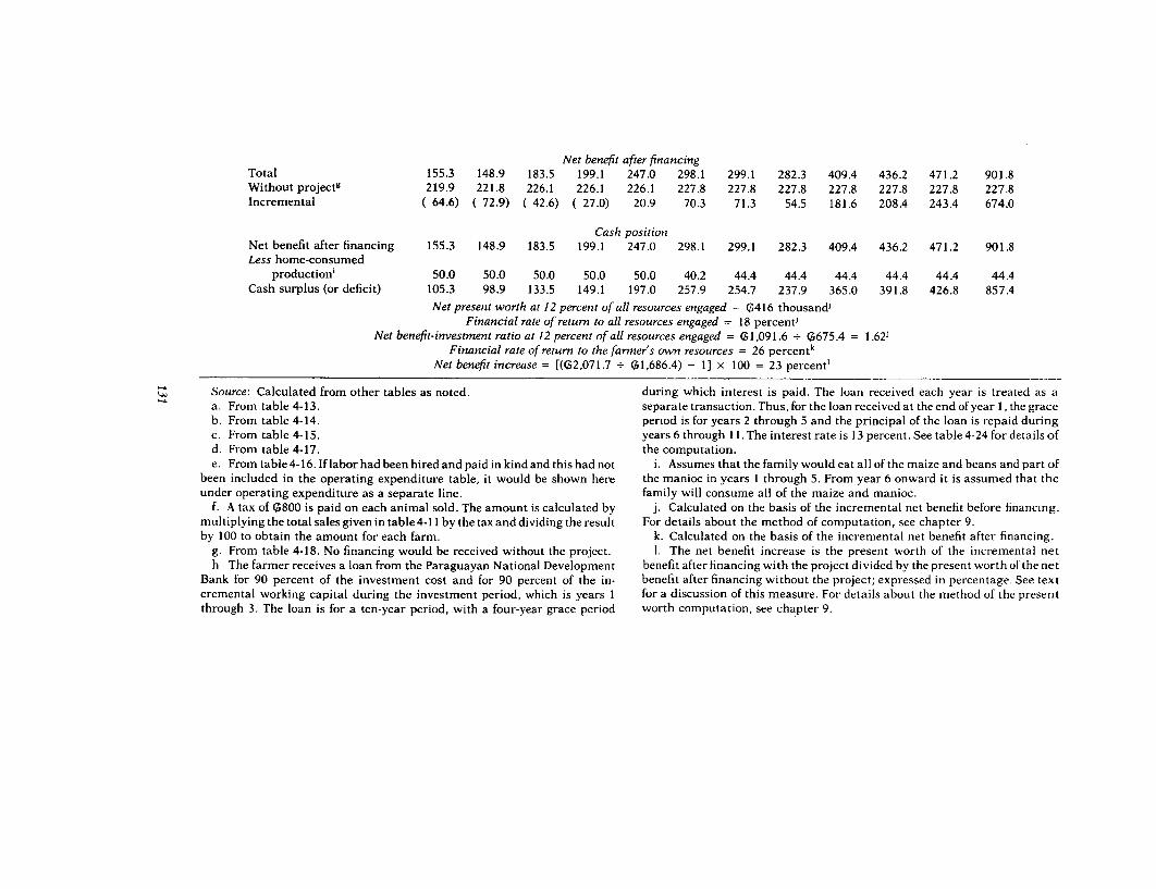
Net benefit after financingTotal 155.3 148.9 183.5 199.1 247.0 298.1 299.1 282.3 409.4 436.2 471.2 901.8Without projectg 219.9 221.8 226.1 226.1 226.1 227.8 227.8 227.8 227.8 227.8 227.8 227.8Incremental ( 64.6) ( 72.9) ( 42.6) ( 27.0) 20.9 70.3 71.3 54.5 181.6 208.4 243.4 674.0
Cash positionNet benefit after financing 155.3 148.9 183.5 199.1 247.0 298.1 299.1 282.3 409.4 436.2 471.2 901.8Less home-consumed
production' 50.0 50.0 50.0 50.0 50.0 40.2 44.4 44.4 44.4 44.4 44.4 44.4Cash surplus (or deficit) 105.3 98.9 133.5 149.1 197.0 257.9 254.7 237.9 365.0 391.8 426.8 857.4
Net present worth at 12 percent of all resources engaged = G416 thousand'Financial rate of return to all resources engaged = 18 percent'
Net benefit-investment ratio at 12 percent of all resources engaged 51,091.6 . Q675.4 = 1.62'Financial rate of return to the fanner's own resources = 26 percentk
Net benefit increase = [(q(2,071.7 . (;1,686.4) - 1] x 100 = 23 percent'
Source: Calculated from other tables as noted. during which interest is paid. The loan received each year is treated as aa. From table 4-13. separate transaction. Thus, for the loan received at the end of year 1, the graceb. From table 4-14. period is for years 2 through 5 and the principal of the loan is repaid duringc. From table 4-15. years 6 through 11. The interest rate is 13 percent. See table 4-24 for details ofd. From table 4-17. the computation.e. From table 4-16. If labor had been hired and paid in kind and this had not i. Assumes that the family would eat all of the maize and beans and part of
been included in the operating expenditure table, it would be shown here the manioc in years I through 5. From year 6 onward it is assumed that theunder operating expenditure as a separate line. family will consume all of the maize and manioc.
f. A tax of ;800 is paid on each animal sold. The amount is calculated by j. Calculated on the basis of the incremental net benefit before financing.multiplying the total salesgiven in table4-1 1 bythetaxanddividingtheresult For details about the method of computation, see chapter 9.by 100 to obtain the amount for each farm. k. Calculated on the basis of the incremental net benefit after financing.
g. From table 4-18. No financing would be received without the project. 1. The net benefit increase is the present worth of the incremental neth. The farmer receives a loan from the Paraguayan National Development benefit after financing with the project divided by the present worth of the net
Bank for 90 percent of the investment cost and for 90 percent of the in- benefit after financing without the project; expressed in percentage. See textcremental working capital during the investment period, which is years I for a discussion of this measure. For details about the method of the presentthrough 3. The loan is for a ten-year period, with a four-year grace period worth computation, see chapter 9.

132 FINANCIAL ASPECTS OF PROJECT ANALYSIS
transaction separately. The timing of the loan receipts, the timing of thedebt service, and the net financing can all be determined easily by simpleinspection. Then, by examining the incremental net benefit after financ-ing, an assessment can be made about the amount of credit a farmer willneed to participate and when he should repay it. With the incrementalnet benefit after financing now available, it is a simple matter to discountit to determine the financial rate of return to the fanmer's own resources.
Of the individual entries included under the inflow in table 4-19, thefirst is the gross value of production, which is derived directly from table4-13. This entry includes only that production available for use off thefarm or by the farm family itself; it does not include any production usedas an intermediate product on the farm. In particular, it does not includefeed produced and fed to animals on the farm. Note the gross value ofproduction includes any production consumed at home; it is not, there-fore, the gross sales. In the Paraguayan example, the family will consumemost of the maize, manioc, and beans it produces, as noted in the lastsection of the farm budget. If we fail to include the value of home-consumed production as part of the gross value of production, we willunderstate the attractiveness to the farmer of participating in the proj-ect. Furthermore, when we recast the budget to reflect economic valueswe will understate the true contribution of the project to the nationalincome. In turn, this will make the measures of project worth of thoseprojects in which a high proportion of the incremental production is to beconsumed by the farm family look relatively less attractive than those ofprojects in which a high proportion of the incremental production is to besold. We may thus penalize many of the very projects that provide thegreatest benefit to the most disadvantaged farmers.
It is important that any off-farn income the farmer may earn beincluded in the budget. Hence, a dummy line has been included in table4-19 even though there is no off-farm income involved in the Paraguayexample. As we will discuss in detail in the next section, by includingoff-farm income in the budget we are automatically able to value familylabor at its opportunity cost. This avoids trying to impute separately anappropriate wage for family labor.
Two other items may enter under the inflow that were not needed inthe Paraguay example. The first is direct grants received by the farmer.Subsidies that benefit the farmer by lowering the cost of an input or byincreasing the price he receives for his production would not be enteredhere. Instead, they would be accounted for by entering the subsidizedmarket price in the account. Later, in the economic analysis, these itemswould have to be revalued to reflect the subsidy.
A second entry that might appear as an inflow in a farm budget but thatis not needed in the Paraguay example is the rental value of the fanmhouse. In most projects, no investment in housing is made, and the rentalvalue remains unchanged with or without the project. As a result, therental value has no effect on the incremental net benefit and so is gener-ally omitted. If, however, the cost of the project has included housing, asmight be the case in a settlement project, then the rental value of thathousing is a benefit for which allowance must be made. In most instances

FARM INVESTMENT ANALYSIS 133
the rental value will be imputed and-as with all imputed values-greatcare must be exercised in determining it.
The last of the inflow items in table 4-19 is the incremental residualvalue. This is derived for the Paraguayan example from table 4-14.
First among the elements of the outflow is the on-farm investment. Notethat the total on-farm investment is included here, not just that propor-tion the farmer is expected to pay from his own funds. The investment thefarmer must make himself as of the end of the year will appear as anegative incremental net benefit after financing at the bottom of the table.For most farm investment analyses, the major items of investment wouldbe detailed in a supporting table such as table 4-15, since the focus sooften is upon some on-farm investment. In projects where the majorinvestment is made off the farm, as might be the case in irrigation, theremay be no substantial on-farm investment.
The next outflow is the incremental working capital, taken from table4-17. As noted earlier in this chapter in the discussion of the accountingconvention, the incremental working capital is calculated as some pro-portion of the increase or decrease in operating expenditure the follow-ing year. It reflects, of course, the need to have on hand at the beginningof the season sufficient funds to finance inputs for crop and livestockproduction.
The next entry for outflow is the operating expenditure, taken from table4-16. If hired labor paid in kind were omitted from table 4-16 (whichsome analysts prefer to treat as a list of cash expenditures), then aseparate entry would have to be included under the operating expenditure.
Finally, an entry is made for other outflows. In the Paraguayan patternfarm budget, the only other outflow is for a tax on cattle sales. A tax onland, however, might also be found under this entry, as might generaloverhead, a betterment levy, or a capital recovery charge for an irriga-tion project. An income tax would usually not be shown here; it isuncommon for a small farmer to have to pay income tax, and, in anyevent, it is generally considered that income tax is levied against thefarmer as an individual rather than against the farm as such. (This, ofcourse, is in contrast to corporate income taxes, which would be shown iflevied; see chapter 5 for a discussion of accounts for agricultural process-ing industries.) In general, indirect taxes such as sales taxes or tariffs onimported items will be included in the price of inputs; this works well forfinancial analysis, but it may lead to complications when the economicvalues are being estimated. The total inflow less the total outflow givesthe net benefit before financing.
The section of table 4-19 devoted to financing begins with the projec-tion of the loan receipts the farmer may expect if he participates in theproject. Loan receipts are commonly divided into short-term andmedium- or long-term. In the Paraguay example, only medium-termloans are to be received. Loans are entered in the year they are to bereceived.
Debt service-the payment of interest and repayment of principal-follows. Usually it, too, will be disaggregated by the length of the loanmaturity. Interest and principal repayments are often shown as a single

134 FINANCIAL ASPECTS OF PROJECT ANALYSIS
entry, although sometimes interest payments and the principal repay-ment are shown separately. The details of how to calculate interestpayments and principal repayments are discussed in the section "Com-puting Debt Service" later in this chapter.
The debt service is subtracted from the loan receipts to reach the netfinancing, which is shown with an indication of whether it is positive ornegative. In the Paraguay example, in years 1 through 3 the loan receiptsexceed the debt service, so the net financing is positive; in years 4 through13, however, debt service exceeds the loan receipts, and so the net financ-ing is negative.
The net financing subtracted from (or added to, as appropriate) the netbenefit before financing gives the net benefit afterfinancing, also called thefarm family net benefit. As noted, this is the amount the family has to liveon with the project and is most important for judging incentive effects ofthe project. It is probably an estimate of this amount that most farmersmake when they decide whether to participate in a project, although nodoubt they arrive at it by a less formal means.
If we subtract the net benefit after financing without the project fromthe net benefit after financing for each project year, we arrive at theincremental net benefit after financing, or incremental farm family netbenefit. This is the same incremental net benefit or cash flow defined inchapter 9. It represents an undifferentiated return of and to the farmer'scapital; discounted, it gives the financial rate of return to the farmer'sown resources. The incremental net benefit after financing also providesus with another basis for a judgment about incentive effects. Would afarmer be willing to shoulder the additional risk and effort needed toparticipate in the project if he can expect this kind of incrementalincome?
Because home-consumed production is included in the farm budget, ifany high proportion of the incremental production is expected to beconsumed in the farm household, it is desirable to have a section on thecash position to determine whether the farmer will have the cash heneeds to purchase modern inputs and to meet his credit obligations. (Thisis the point at which a bit of funds flow analysis is mixed in with the farminvestment analysis.) One means is to calculate a separate cash budget asBrown suggests (1979, pp. 25-30). Another means is shown at the bottomof table 4-19. Here, a line is added to subtract the value of home-consumedproduction from the net benefit after financing. The remainder is the cashsurplus (or deficit). If there is a deficit, it must be made up from familysavings or other sources if the farmer is not to fall behind in his invest-ment plan or to default on his credit obligations. Alternatively, we maywish to adjust the amount of short-term credit extended or alter theconditions of long-term credit to avoid the cash deficit.
The farm budget presented in table 4-19 assumes that the real burdenof debt service will continue throughout the life of the loan the farmerreceives. As in most countries, in the Paraguay project the lending termsto farmers call for repayment in nominal-that is, money-terms. In-terest is stated at a given rate, and the nominal amount of principalrepayment is agreed upon. If, however, a country experiences inflation

FARM INVESTMENT ANALYSIS 135
that reduces the real value of money over time, the result is that farmerswhose debt service payments are fixed in money terms have a decliningreal burden of debt service. Some countries try to adjust for this byindexing loans so that the nominal amount a farmer pays changes tomaintain the same real burden of debt service, but most do not.
If Paraguay were expected to experience inflation, then the farmbudget would be a more realistic indicator of income and incentive if itreflected the declining real burden of debt service. Predicting futureinflation rates is difficult at the very least (and may lead to politicalcomplications for analysts in public agencies if the government hasadopted a strong anti-inflation program). Past experience is some indica-tion of what future inflation may be. In 1977 the wholesale price index inParaguay rose by 8 percent, so that rate might be accepted as an estimateof future inflation. If we assume constant inflation of 8 percent during thelife of the loan, then the debt service each year will be reduced bydividing it by 1 plus the rate of inflation stated in decimal terms to reflectthe declining real burden. The farm budget for the Paraguay example isrecast in table 4-20 to incorporate this assumption. The table projectsthat the real value of the loan receipts in years 2 and 3 will remain thesame-which is to say that their nominal value will increase by theamount of inflation. This is perhaps an unrealistic assumption in manycountries. If so, not only the debt service but the real value of the loanreceipts might be reduced by the amount of the inflation, and the farmerwould have to invest more of his own resources to keep his investmentprogram on schedule. (The details about how the loan receipts and debtservice were calculated are given in the section "Computing Debt Ser-vice" and in table 4-26, below.)
The recast farm budget in table 4-20 begins with the net benefit beforefinancing, which is the same as that in table 4-19 since table 4-19 is cast inconstant terms and the relative prices are correct. (The reader will recallthat the prices in table 4-12, which formed one of the bases for table 4-19,were varied to allow for changing relative values.) Since all prices in bothtables 4-19 and 4-20 maintain the same relation to each other or havebeen changed to reflect changing relations, the tables are, in effect, cast interms of the value of the guarani in project year 1. The terms of the loan tothe farmer from the Paraguayan National Development Bank are thesame as those outlined in table 4-19 and are set in nominal terms.Comparing the debt service line in tables 4-19 and 4-20 shows the effect ofassuming a declining real burden of debt service, as does a comparisonbetween the two lines for the incremental net benefit after financing.
Recasting the farm budget to reflect the declining real burden of debtservice shows that the real return to the farmer for his own resourceswould rise from the 26 percent estimated in table 4-19 to 34 percent. Thenet benefit increase (discussed later in this chapter) would rise from 23percent to 35 percent. Both increases, of course, reflect the declining realburden of the debt service.
Casting the farm budget to reflect the declining real burden of debtservice that occurs in inflationary circumstances certainly is more realis-tic than assuming a constant burden. It probably also will lead to a better

Table 4-20. Farm Budget Assuming Declining Real Burden of Debt Service, 20-Hectare Mixed Farm, Paraguay Project
(thousands of C)
Project year
Item 1 2 3 4 5 6 7 8 9 10 11 12 13 14-19 20
Net benefit before financing' (359.2) 107.9 123.5 297.3 345.2 457.3 471.2 471.2 471.2 471.2 471.2 471.2 471 2 471.2 901.8
FinancingbLoan receipts' 508.2 107.1 140.0 0 0 0 0 0 0 0 0 0 0 0 0
Debt servicec - 61.2 69.6 81.3 75.2 111.1 111.6 114.9 106.3 98.4 91.1 29.8 16.2 0 0
Net financing 508.2 45.9 70.4 ( 81.3) ( 752) (111.1) (111 6) (1149) (106.3) ( 98.4) ( 91.1) ( 29.8) ( 16.2) 0 0
Net benefit after financingTotal 149.0 153.8 193.9 216.0 270.0 346.2 359.6 356.3 364.9 372.8 380.1 441.4 455.0 471.2 901.8
Without project' 219.9 221.8 226.1 226.1 226.1 227.8 227.8 227.8 227.8 227.8 227.8 227.8 227.8 227.8 227.8
Incremental ( 70.9) ( 68 0) ( 32.2) ( 10.1) 43.9 118.4 131.8 128.5 137.1 145.0 152.3 213.6 227.2 243.4 674.0

Cash positionNet benefit after financing 149.0 153.8 193.9 216.0 270.0 346.2 359.6 356.3 364.9 372.8 380.1 441.4 455.0 471.2 901.8Less home-consumed
productiona 50.0 50.0 50.0 50.0 50.0 40.2 44.4 44.4 44.4 44.4 44.4 44.4 44.4 44.4 44.4Cash surplus (or deficit) 99.0 103.8 143.9 166.0 220.0 306.0 315.2 311.9 320.5 328.4 335.7 397.0 410.6 426.8 857.4
Net present worth at 12 percent of all resources engaged = (;416 thousand'Financial rate of return to all resources engaged = 18 percentd
Net benefit-investment ratio at 12 percent of all resources engaged = l ,091.6 -- 675.4 = 1.62dFinancial rate of return to the farmer's own resources = 34 percent'
Net benefit increase = [(02,282.3 - (i1,686.4) - 1] x 100 = 35 percent'
Source: Calculated from other tables as noted. c. For details of the computation, see the section "Computing Debt Service" anda. From table 4-19. table 4-26 later in this chapter.b. The terms and conditions of the financing are assumed to be the same as those d. Calculated on the basis of the incremental net benefit before financing. (Notein table4-19, noteh.Itis assumed that therewill beaconstant inflationof8 percent that this is the same value as in table 4-19). For details about the method ofduring the term of the loans. The table is stated in real terms in constant guaranis of computation, see chapter 9.
project year I (except for the nominal terms for the loan receipts). Since debt service e. Calculated on the basis of the incremental net benefit after financing.is denominated in nominal (money) terms, the real burden declines each year by the f. The net benefit increase is the present worth of the incremental net benefitamount of inflation. Loan receipts are stated in real terms under the entry for loan after financing with the project divided by the present worth of the net benefit afterreceipts, and the nominal amounts for the second and third-year loans are given. financing without the project expressed in percentage. See text for a discussion ofThe nominal amount is increased by the amount of inflation. this measurement. For details about the method of computing the present worth,see chapter 9.

138 FINANCIAL ASPECTS OF PROJECT ANALYSIS
estimate of the real attractiveness of a project to farmers, since mostfarmers will have some sense of the effect of inflation on nominal values.Except for the additional computations needed to project the farmbudget, such an approach creates no analytical complications. Projectaggregations can simply be based on the farm budgets that assume adeclining real burden of debt service, just as they would be if the budgetassumed that the burden of the debt service would remain constant andthat the loan would be indexed. Of course, allowing for a declining realburden of debt service in the farm budget would not change the economicrate of return of a project, since that is based on the net benefit beforefinancing valued in economic terms (discussed in chapter 7).
COST OF FAMILY LABOR. A common conceptual problem met when pre-paring farm investment analyses is how to determine the cost of familylabor. The general principle, as with most questions of valuation, is tovalue family labor at its opportunity cost; that is, the benefit the familymust forgo to participate in the project. This is done simply and moreor less automatically if the farm budget format recommended here isfollowed.
This method has the tremendous practical advantage that the cost offamily labor need not be estimated directly. Rather, the cost of familylabor is taken to be what the family could earn in its next most remunera-tive alternative without the project. To accomplish this, the farm budgetmust compare the with-project situation with the without-project situa-tion, and the off-farm labor income must be included in the budget-atleast if there is to be any change in the amount earned from off-farmlabor. The cost of the family labor needed to adopt the with-projectcropping pattern, then, is the labor income in the without-project situa-tion that must be given up. If the number of days of off-farm work must bereduced for the farm family to participate in the project, to that extentthe cost of incremental family labor is the off-farm wage. If the with-project cropping pattern calls for a shift of family labor from one produc-tion activity on the farm to another, the cost of the labor shifted isimplicitly set at the labor income forgone in the without-project activity.Finally, if more total family labor is called for in the with-project crop-ping pattern than in the pattern without the project, as is the case in theParaguay example, this additional labor is implicitly priced at an oppor-tunity cost of zero, since no income must be forgone to use the labor in thewith-project cropping pattern. This assumes, in effect, that the familywould have worked more days of the year in the without-project situa-tion had there been suitable opportunities available either through addi-tional farm work or off the farm. Any incremental labor needed in thewith-project cropping pattern compared with the without-project crop-ping pattern plus off-farm employment is assumed to be taken fromundesired leisure given up. (Later, when the analyst converts from finan-cial prices to economic values, the off-farm earning would be valued atthe appropriate shadow wage.)

FARM INVESTMENT ANALYSIS 139
If the family would not, in fact, give up leisure for the amount it couldearn from additional farm labor by participating in the project, then theproposed cropping pattern is unrealistic and should not be used. Such asituation could easily arise. In many societies, the period just afterharvest is a time of family festivals. A proposed cropping pattern callingfor substantial family labor during this time would in all likelihood beunacceptable to the farmers. In effect, we are saying that the family has a" reservation price" for leisure-the price at which the family is willing togive up leisure for additional work-that is greater than the return thefamily would receive for working the additional work days. Note that wedo not attempt in this process to determine any value for leisure time. Allwe are saying is that the reservation price for leisure is greater than thereturn the family can earn from the proposed project's cropping pattern.
Of course, the reservation price for leisure will vary widely with thecircumstances. For substantially unemployed rural labor, the reserva-tion price may be quite low. But if every adult family member is alreadyengaged some 200 days a year, then the reservation price for labor justafter the harvest season may be rather high, for continued labor at thistime may mean missing treasured family occasions. As the number ofdays of labor approaches the physical maximum, the reservation pricewill rise until almost no return is great enough to elicit additional labor.
If we lay out the pattern farm budgets as suggested here, and familylabor is valued at its opportunity cost, there is no need to have a separateentry for the value of family labor. To have such an entry amounts todouble counting. Even so, because many analysts are uncomfortablepresenting a budget with no directly identified allowance for familylabor, a separate value for family labor is commonly found to be includederroneously in agricultural project analyses.
COST OF LAND. A parallel approach to that suggested for the opportu-nity cost of family labor may be taken to determine the cost of land. Thisis especially convenient whenever the project does not contemplate achange in ownership but rather a change only in land use. If farmers shiftfrom rainfed sorghum to irrigated rice without changing the land own-ership, as has happened in several agricultural projects along the majorrivers of West Africa, the cost of the land is its contribution to the value ofthe sorghum production that the farmers must forgo to use the land forrice. This is automatically provided for when we lay out the farm budgetto show the difference with and without the project. Therefore, a separateentry for the cost of land is not needed, either in the financial or in theeconomic accounts.
When there is a separate rent paid by the farm family for the use of theland, then the rent is properly shown as a cost in the financial analysis-in both the without-project and the with-project situations-since itreduces the net benefit available to the family. However, when we con-vert this budget to efficiency prices for the economic analysis, as dis-cussed in chapter 7, simply casting the economic account on a with and

140 FINANCIAL ASPECTS OF PROJECT ANALYSIS
without basis without entering the rent separately would be the simplestway to allow for the opportunity cost of land.
If the land is to be purchased, the purchase price would properly beshown as a cost in the financial accounts. Again, however, in convertingto efficiency prices for the economic analysis the opportunity cost wouldbe taken as the economic value. As before, simply comparing the situa-tions with and without the project in the economic accounts is generallythe most convenient approach and will correctly value the land at itsopportunity cost. Sometimes, however, different approaches may betaken in the economic accounts, a topic to which we will return inchapter 7 in the subsection "Step 3. Adjustment for price distortions innon-traded items."
Net Benefit Increase
We should note that, although the farm budgets given in this chapterplace a fair amount of stress on determining the net present worth, thefinancial rate of return, and the net benefit-investment ratio to the farm-er's own resources, these measures of project worth are in fact not veryimportant to the farmer. Far more important to farmers is the actualamount of additional income they expect to receive. It is probably fair tosay that for most small farmers the concept of capital return hardly playsany part in their decision. Indeed, in many farm budgets these measuresof project worth are almost meaningless. For example, in the ThirdAgricultural Credit Project in Kenya, for the model ii smallholder in farmzone B, the return to the farmer's own capital resources is extremelyhigh. This is so because it is proposed to lend to the farmer most of thecost of the incremental investment for a new dairy enterprise, and theincremental return from the new enterprise from year 2 onward is suf-ficient to make the incremental net benefit after financing positive. Thus,the farmer really needs very little in the way of his own capital resourcesto participate in the project, although he will still have to bear most ofthe risk. Despite the high rate of return, since the farmer's own capitalcontribution is small, the absolute amount of his return is also small.Indeed, the whole incremental net benefit after financing, or incrementalfarm family net benefit, is not all that great. Hence, no one would worryabout the apparently very high windfall return the farmer would receiveon his own capital resources engaged in the project.
Farmers probably pay more attention to the potential increase in theirincremental net benefit after financing, so it is convenient to have ameasure that succinctly describes what that is. Schaefer-Kehnert (1980)has proposed the net benefit increase for this purpose. This is the presentworth of the incremental net benefit after financing with the project,divided by the present worth of the net benefit after financing without theproject, expressed in percentage terms. (The mechanics of determiningthe present worth are discussed in chapter 9.) In the farm budget for theParaguay project pattern farm given in table 4-19, for example, at a 12

FARM INVESTMENT ANALYSIS 141
percent discount rate the present worth of the incremental net benefitafter financing with the project is 02,071.7 thousand, and the presentworth of the net benefit after financing without the project is 01,686.4thousand. The net benefit increase, thus, is 23 percent {[(2,071.7. 1,686.4) - 1] x 100 = 23}. The net benefit increase may be interpreted
as the weighted average incremental increase in income the farmer willreceive over the life of the project if he participates. The net benefitincrease provides a basis for determining whether the increased incomewill be sufficient to attract farmers' participation in a project and forcomparing easily the relative attractiveness to farmers of alternativeproject possibilities.
Unit Activity Budgets
We have discussed in considerable detail preparation of whole farmbudgets for farm investment analysis. This generally is the preferableanalytical approach in agricultural project analysis. An alternativeapproach, however, is to prepare a "unit activity budget"; that is, abudget which applies only to some particular investment activity-say, ahectare of fruit trees or a broiler chicken production unit. This approachis related to the "partial" budgeting commonly used by farm manage-ment specialists in that it examines the return to a single activity on thefarm rather than to the farm as a whole, with that one activity incorpo-rated in the cropping pattern. Brown discusses partial budgets for agri-cultural project analysis (1979, pp. 25-30).
Unit activity budgets are particularly convenient when a project fo-cuses on a single crop or livestock activity. Often these activities areconsidered as additions to existing farm activities that will encourageincreased output of the commodity in question and will increase farmincomes. Usually it is thought that the activity can be added to theongoing farm cropping pattern without disruption and without seriouslyreducing the resources available for other activities on the farm. Ratherthan develop a range of pattern whole farm budgets incorporating thenew activity, many analysts choose simply to do a unit activity budgetshowing the cost and return per unit to the individual farmer who adoptsthe innovation and then to aggregate by multiplying the results by thenumber of hectares or of livestock production units to be included in theproject. Unit activity budgets are used to good advantage where spec-ification of opportunity costs for land or labor is not crucial. They may beused when estimating the area is difficult or inappropriate and where it isconsidered that the labor involved will not be seriously competitive withother farm activities. They have been used, for example, as the basis foragricultural project analysis where the objective was to encourage small-scale planting of grapes for raisin production in Afghanistan, to encour-age stall feeding of cattle in Kenya, and to encourage the addition of asmall dairy enterprise to existing farms in India. Unit activity budgets

142 FINANCIAL ASPECTS OF PROJECT ANALYSIS
have the advantage of generally being easier to prepare, since it is notnecessary to collect and analyze information on any farm productionactivity other than the one to be encouraged in the project.
There are, however, significant limitations in unit activity budgets.The most important is that they fail to assess the effect of undertaking anew activity on the resource use of the farm and on overall farm income.In the absence of whole farm budgets, the analyst may give too littleattention to the place of a proposed innovation in the cropping pattern ofthe entire farm and thus make an erroneous judgment about incentiveeffects. It may be overlooked that incorporating a particular crop orinnovation in the farm as a whole may cause labor shortages arisingeither from competition for family labor or for the total labor supply inthe area. The analyst may fail to appreciate the competition for land of anew crop with other crops grown on the farm. Using unit activity budgetsinstead of whole farm budgets also reduces the analyst's ability to assessthe farmer's credit need and repayment capacity, which are influencednot only by the incremental income from a particular production innova-tion but also by the financial position of the farm as a whole.
A major problem with unit activity budgets is that it is easy to overlookopportunity costs or to value them erroneously. One substantial advan-tage of laying out whole farm budgets in the manner suggested in thischapter is that this method correctly allows for the opportunity cost ofland and labor-including, most importantly, family labor. Unit activitybudgets generally are done directly on an incremental basis, rather thancast in a with-and-without form. This means that all opportunity costsmust be estimated directly to obtain the incremental net benefit, andgreat care must be taken to see that they are correctly estimated. Concep-tually, of course, if the opportunity costs are correctly stated, there willbe no difference in the estimated incremental net benefit, either to theindividual farmer or to the society as a whole, whether the basis is awhole farm budget or a unit activity budget. In practice, however, thesituation is quite different. Both the opportunity cost of the land to beused for the new crop or livestock undertaking and the opportunity costof family labor must be imputed rather than derived from establishedmarket prices. Such estimates are difficult to make correctly; they arefrequently in error and will give results that will differ from those thatwould be obtained by using whole farm budgets. (The full "partial"budgeting technique developed by farm management specialists canalso be used for estimating the opportunity cost of land and labor, but thefull approach is not often used in practice for agricultural projectanalysis.)
We may illustrate a unit activity budget with an example drawn fromthe Indian Cashewnut Project. The project is to help finance a cashewproduction program in four Indian states; the project includes 35,000hectares to be developed by smallholders. The project analyst chose touse the unit activity approach because most cashews in India are grownby smallholders in small clumps, in hedgerows, or as backyard trees.Preparing pattern whole farm budgets that reasonably represented the

FARM INVESTMENT ANALYSIS 143
range of possible combinations of farm sizes and cashew productionactivities would entail a large number of examples. Instead, six unitactivity budgets for a hectare of cashews each were prepared for newplantings and two for rehabilitation of existing plantings. The in-cremental net benefit from each unit activity budget was then multipliedby the area foreseen in the project for each pattern to obtain the contribu-tion to the total project benefit of increased cashew production by small-holders.
The relevant background information to the Indian project is given intable 4-21. This gives the value of production and the investment andoperating expenditure. (The symbol for Indian rupees is Rs.) In the budgetas prepared by the analyst, no distinction was made between investmentand operating expense; instead, both were simply defined as "produc-tion" cost, a conceptually correct approach. To keep this presentationparallel to that for the Paraguay whole farm budget discussed earlier inthis chapter, however, all expenditure before the trees begin to bear israther arbitrarily considered investment, whereas that incurred afterbearing begins is considered operating expenditure. The advantage ofthis treatment is that it makes it analytically convenient to calculate theincremental working capital needed. In the summary reproduced here,the details about the amounts and unit prices of the materials needed,which were included in the original project analysis, have been omittedto conserve space.
The background information points up some of the problems of usingthe unit activity approach to budgeting. Among the investment andoperating expenditures, the analyst has indeed included all the oppor-tunity costs. Both the opportunity cost for land and for labor wereestimated directly. In the Indian Cashewnut Project, the trees areassumed to be planted in areas otherwise put to no economic use; theopportunity cost of the land can thus be appropriately taken as zero. Inother instances, however, the opportunity cost of the land might bepositive, and the points we have made earlier in the "Farm budget"subsection about estimating the opportunity cost of land would have tobe considered. It might be appropriate, for instance, to use rent as anestimate of the contribution of land to the value of production forgone toundertake the new activity. In still other instances, the purchase price ofthe land might appropriately account for its opportunity cost, eventhough purchase price is generally a poor estimate. This might be thecase in a livestock-fattening project, for instance, where the area in-volved is small and the opportunity cost of the land is minor in relation tooverall costs, so that using the purchase price would not lead to a signif-icant error in the investment decision. Finally, in some instances it mayprove necessary to estimate the contribution of the land to the forgoneproduction directly, say, by assigning the residual after deducting allother costs from the value of production to land. This might be the case iffarmers are expected to shift some of the land they already crop toanother production activity.
Another problem with the unit activity budget approach is pointed up

Table 4-21. Value of Production, Investment, and Operating Expenditure,1-Hectare Planting Model, Cashewnut Project, Smallholder Component, Karnataka, India
Project year
Item 1 2 3 4 5 6 7 8 9 10 11-40
Value of productionYield (kg/ha) 0 0 0 50 150 400 600 700 800 900 900Price' (Rs/kg) - - - 4.1 4.2 4.3 4.4 4.6 4.8 4.9 5.1Gross value of production (Rs) 0 0 0 205 630 1,720 2,640 3,220 3,840 4,410 4,590
Investment and operating expendtturebLand
Rent (opportunity cost) (Rs)' 0 0 0 0 0 0 0 0 0 0 0Total land (Rs) 0 0 0 0 0 0 0 0 0 0 0
Labor (work days)Land clearing, development 70 0 0 0 0 0 0 0 0 0 0Pit digging 15 0 0 0 0 0 0 0 0 0 0Planting seedl]ngs 6 0 0 0 0 0 0 0 0 0 0Crescent bunding 0 25 25 0 0 0 0 0 0 0 0Ringweeding 0 20 15 0 0 0 0 0 0 0 0Gap filling 0 1 0 0 0 0 0 0 0 0 0Bund maintenance 0 0 0 4 5 5 5 5 5 5 5

Mulching, weeding, watering 10 0 10 20 15 12 10 10 10 10 10Fertilizer application 4 5 5 5 5 5 5 5 5 5 5Plant protection 2 2 4 5 9 10 10 10 10 10 10Harvesting 0 0 0 3 10 16 24 28 32 36 36Miscellaneous 3 3 3 3 5 5 5 5 5 5 5
Total labor 110 56 62 40 49 53 59 63 67 71 71Wage (Rs/day) 8 8 8 8 8 8 8 8 8 8 8Labor cost (Rs) 880 448 496 320 392 424 472 504 536 568 568
Materials' (Rs)Plant materials 50 10 0 0 0 0 0 0 0 0 0Fertilizer 150 250 350 400 400 400 400 400 400 400 400Plant protection 40 80 120 150 175 175 175 175 175 175 175Miscellaneous 20 20 20 20 20 20 20 20 20 20 20
Total materials 260 360 490 570 595 595 595 595 595 595 595Total investment 1,140 808 986 0 0 0 0 0 0 0 0
Total operating expenditure 0 0 0 890 987 1,019 1,067 1,099 1,131 1,163 1,163
Rs Indian rupees; kg. kilograms. b. The analyst of the project did not distinguish between investment andSource: Adapted from World Bank, "India, Cashewnut Project, Staff operating expenditure, preferring instead to treat both simply as "produc-
Appraisal Report," 2437-IN (Washington, D.C., 1980; restricted circulation), tion" cost. Production cost in years I to 3 before the trees bear is taken to beannex 4, table 1. investment, in years 4 to 40 to be operating expenditure.
a. Based on projected f.o.b. price adjusted to give the export parity value at c. Trees are assumed to be planted in areas that otherwise would be put tothe farm gate. Details given in the original project report, from which this no economic use.example is drawn, are not reproduced here. d. Details of application rates and prices given in the original project report
are not reproduced here.

146 FINANCIAL ASPECTS OF PROJECT ANALYSIS
by the background information. Labor represents a high proportion ofthe operating expenditure, characteristically on the order of half. Laborhas been valued at a daily wage of Rs8, and this in turn was shadow-priced in the economic analysis at 70 percent of the market rate to allowfor rural unemployment along the lines discussed in chapter 7. But, sincemost of the smallholder plantings will be in very small areas, evenbackyards, it is likely that family members will do most of the work. Andthey will probably do this at odd times, when they otherwise do not haveopportunities for productive employment either on their own holdings oras hired labor. Thus, the opportunity cost to the family may be close tozero and the incremental net benefit correspondingly larger, making theproject that much more attractive to farmers and reducing the need forcredit. Similarly, when converting the financial prices to economicvalues along the lines discussed in chapter 7, if much of the labor issupplied by the family at times when there are no other opportunities forproductive employment, then the economic value of the labor may alsobe close to zero-and the economic attractiveness of the smallholdercomponent of the project that much more attractive from the standpointof the economy as a whole.
The unit activity budget is given in table 4-22. Its format follows thatadopted for the whole farm budget. From the inflow (including a subsidyfor planting) is subtracted the outflow to obtain the incremental net benefitbefore financing. Discounted, this will give the net present worth, finan-cial rate of return, or net benefit-investment ratio to all resources en-gaged. Changing the financial prices to economic values and omittingtransfer payments (see chapter 7) will give the incremental net benefit ineconomic terms. This may then be aggregated by multiplying by thenumber of units expected in the project to give the total incremental netbenefit contributed to the project by the on-farm production.
Proceeding to the financing, loan receipts less debt service give the netfinancing. The terms and conditions of the loans are given in the notes tothe table. (A detailed exposition of how the debt service was calculated isgiven, in the subsection on computing debt service, using "equal install-ments with interest capitalized," later in this chapter.) The com-putation is made more complex because the interest is capitalized duringthe investment period. Also, the interest rate for the loan is 10.5 percent,and many discounting tables do not give factors for high fractionalinterest rates. The relevant factors, however, may easily be calculated ona simple hand calculator (as discussed in chapter 10 under "CalculatorApplications in Project Analysis"). These credit estimates again raise theproblem of estimating opportunity costs. The amount of credit is calcu-lated assuming that the farmer will pay Rs8 per day for all the laborengaged. But if family labor were used for which the opportunity costwere lower, perhaps even zero, then the farmer would not need so muchcredit to undertake the new activity. Were credit extended on the basis ofthe unit activity budget, there might be more lent than necessary tofurther the project, and there would be significant "leakage." This couldbe avoided by a credit agency if its staff made separate analyses for each

FARM INVESTMENT ANALYSIS 147
borrower based on the borrower's real costs rather than simply applyinga rule of thumb derived from the unit activity budget.
Finally, we reach the entry for incremental net benefit after financing.Discounted, this will give the financial rate of return to the farmer's ownresources, assuming that the farmer invested his own capital in theproject as indicated in the budget and that all costs have been correctlyestimated.
Computing Debt Service
In many farm budgets there will be a credit element, and the analystwill have to calculate the amount of the debt service. In this section, wewill briefly review how to compute the amount of interest due and theamount of the principal repayment for four different repayment terms.We will also consider how to adjust for the declining real burden of debtservice when there is inflation. Computations will be carried to thenearest whole currency unit or to some other convenient rounding aggre-gate, since that is the common practice in most farm budgets used inproject analysis. Credit agencies, of course, will have to work to thenearest unit in common use for commercial transactions: cents, paise,nguawa, or whatever.
In the examples given here, where the term of the loan is a year orlonger we will follow the accounting convention adopted-that loans areto be received at the end of a project year and that debt service is to beginin the following year. Often in project accounts, however, the analyst willchoose to assume that the loan is made at the beginning of the accountingperiod and that debt service is paid at the end. As noted, this leads to theanomaly that for a loan of a year or longer both the loan receipt and thefirst interest payment, and perhaps even the first principal repayment,are shown within the same project year. It can also lead to an understate-ment of the short-term credit the farmer will need and to an overstate-ment of his financial rate of return.
Simple interest
The easiest term to calculate, of course, is common simple interestsuch as that found in short-term credit lent for seasonal expenses. In theKenya Third Agricultural Credit Project, for example, the farmer re-ceives a loan in year I of KShl,374, which he is to repay twelve monthslater at 11 percent interest. (The symbol for Kenyan shillings is KSh.)Thus, the interest is KShl51 (1,374 x 0.11 = 151). The total amount to berepaid by the Kenyan farmer is the principal borrowed plus the interest,or KShl,525 (1,374 + 151 = 1,525). If we are concerned only about thetotal amount to be repaid and do not need to separate interest andprincipal, as is often the case in preparing farm budgets, then it is simplerto calculate the total repayment in one step by multiplying the principal

Table 4-22. Unit Activity Budget, 1-Hectare Planting, India Cashewnut Project(Rs)
Project year
Item 1 2 3 4 5 6 7 8 9 10 11-13 14-39 40
InflowGross value of production' 0 0 0 205 630 1,720 2,640 3,220 3,840 4,410 4,590 4,590 4,590
Subsidyb 300 300 300 0 0 0 0 0 0 0 0 0 0
Incremental residual value' - - - - - - - - - - - - 1,163
Total 300 300 300 205 630 1,720 2,640 3,220 3,840 4,410 4,590 4,590 5,753
OutflowInvestmenta 1,140 808 986 0 0 0 0 0 0 0 0 0 0
Incremental working capitald - - 890 97 32 48 32 32 32 0 0 0 0
Operating expenditure' - - - 890 987 1,019 1,067 1,099 1,131 1,163 1,163 1,163 1,163
Other 0 0 0 0 0 0 0 0 0 0 0 0 0
Total 1,140 808 1,876 987 1,019 1,067 1,099 1,131 1,163 1,163 1,163 1,163 1,163
Incremental net benefitbefore financing ( 840) ( 508) (1,576) ( 782) ( 389) 653 1,541 2,089 2,677 3,247 3,427 3,427 4,590

Financing'Loan receipts 783 468 1,482 733 338 0 0 0 0 0 0 - -
Debt service 0 0 0 0 0 499 499 1,108 1,108 1,108 1,108Net financing 783 468 1,482 733 338 ( 499) ( 499) (1,108) (1,108) (1,108) (1,108)
Incremental net benefitafter financing ( 57) ( 40) ( 94) ( 49) ( 51) 154 1,042 981 1,569 2,139 2,319 3,427 4,590
Net present worth at 12 percent of all resources engaged = Rs 9,324fFinancial rate of return to all resources engaged = 29 percentf
Net benefit-investment ratio at 12 percent of all resources engaged = 12,318 . 2,994 = 4.1 fFinancial rate of return to the farmer's own resources = >50 percentg
Source: Same as table 4-21. subsidy received and less the gross value of production in years when the neta. From table 4-21. benefit before financing is negative. In year 4, for example, the amount of theb Participatingsmallholdersreceivea25percentsubsidyofthecostofnew loan is 95 percent of the incremental working capital plus the operating
planting or Rs900 per hectare, whichever is less. expenditure less the gross value of production {[0.95(97 + 890)] - 205 = 733}.c. The incrementalresidualvalueconsistsentirelyoftheworkingcapital.It Loans extend for twelve years, including a six-year grace period beginning
is assumed the trees have no residual value at the end of the project. with the year after the first loan is made. That is, repayment of all loans beginsd. The incremental working capital is calculated on the assumption that all in year 8 after termination of the six-year grace period from years 2 through 7.
operating expenditure should be taken as the basis for the calculation. For Interest is capitalized during the period of disbursement; interest only is paideach year 100 percent of the incremental operating expenditure is taken as in years 6 and 7; and equal installments of debt service are made from years 8recommended in table 4-3. This makes the implicit assumption that the labor through 13. See the section "Computing Debt Service" and table 4-25 for ancost represents an accurate estimate of the opportunity cost of the family labor explanation of how the calculations are made.used. See text for discussion. f. Calculated on the basis of the incremental net benefit before financing.
e. Participating smallholders may borrow 95 percent of investment, in- For details about the method of computation, see chapter 9.cremental working capital, and operating expenditure less the amount of g. Calculated on the basis of the incremental net benefit after financing.
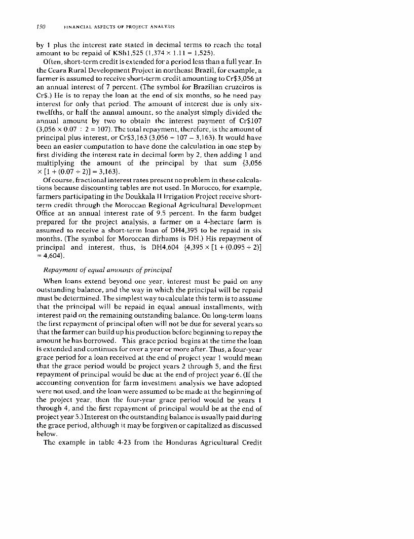
150 FINANCIAL ASPECTS OF PROJECT ANALYSIS
by 1 plus the interest rate stated in decimal terms to reach the totalamount to be repaid of KSh 1,525 (1,374 x 1.11 = 1,525).
Often, short-term credit is extended for a period less than a full year. Inthe Ceara Rural Development Project in northeast Brazil, for example, afarmer is assumed to receive short-term credit amounting to Cr$3,056 atan annual interest of 7 percent. (The symbol for Brazilian cruzeiros isCr$.) He is to repay the loan at the end of six months, so he need payinterest for only that period. The amount of interest due is only six-twelfths, or half the annual amount, so the analyst simply divided theannual amount by two to obtain the interest payment of Cr$107(3,056 x 0.07 + 2 = 107). The total repayment, therefore, is the amount ofprincipal plus interest, or Cr$3,163 (3,056 + 107 = 3,163). It would havebeen an easier computation to have done the calculation in one step byfirst dividing the interest rate in decimal form by 2, then adding 1 andmultiplying the amount of the principal by that sum {3,056x [1 + (0.07 + 2)] = 3,163}.
Of course, fractional interest rates present no problem in these calcula-tions because discounting tables are not used. In Morocco, for example,farmers participating in the Doukkala II Irrigation Project receive short-term credit through the Moroccan Regional Agricultural DevelopmentOffice at an annual interest rate of 9.5 percent. In the farm budgetprepared for the project analysis, a farmer on a 4-hectare farm isassumed to receive a short-term loan of DH4,395 to be repaid in sixmonths. (The symbol for Moroccan dirhams is DH.) His repayment ofprincipal and interest, thus, is DH4,604 {4,395 x [1 + (0.095 + 2)]= 4,604}.
Repayment of equal amounts of principal
When loans extend beyond one year, interest must be paid on anyoutstanding balance, and the way in which the principal will be repaidmust be determined. The simplest way to calculate this term is to assumethat the principal will be repaid in equal annual installments, withinterest paid on the remaining outstanding balance. On long-term loansthe first repayment of principal often will not be due for several years sothat the farmer can build up his production before beginning to repay theamount he has borrowed. This grace period begins at the time the loanis extended and continues for over a year or more after. Thus, a four-yeargrace period for a loan received at the end of project year 1 would meanthat the grace period would be project years 2 through 5, and the firstrepayment of principal would be due at the end of project year 6. (If theaccounting convention for farm investment analysis we have adoptedwere not used, and the loan were assumed to be made at the beginning ofthe project year, then the four-year grace period would be years 1through 4, and the first repayment of principal would be at the end ofproject year 5.) Interest on the outstanding balance is usually paid duringthe grace period, although it may be forgiven or capitalized as discussedbelow.
The example in table 4-23 from the Honduras Agricultural Credit

FARM INVESTMENT ANALYSIS 151
Project, taken from a pattern farm budget for a 50-hectare beef-fatteningunit, illustrates the debt service computation on a loan for which theprincipal is to be paid in equal amounts and interest is to be paid on theoutstanding balance. The computation when the budget assumes ouraccounting convention for farm investment analysis is shown in the firstpart of the table. The farmer is to be loaned a total of L12,699 in threeinstallments during the first three years of the project. (The symbol forHonduran lempiras is L.) For the first installment he is allowed a three-year grace period, for the second a two-year grace period, and for thethird a one-year grace period. Then he is to repay his loan over a three-year period from years 5 through 7. The principal is to be repaid in threeequal installments of L4,233 (12,699 . 3 = 4,233). (In the actual project,the analyst chose to change the principal repayments slightly to makethe loan balance a round figure.) The interest rate is 11 percent a year.The interest paid in year 3, for instance, is computed on the basis of theloan of L3,123 received at the end of year 2 plus the loan of L7,767received at the end of the first year that is still outstanding, or a totalprincipal on which interest is to be paid of L10,890. The interest due isL 1,198 [(7,767 + 3,123) x 0.11 = 1,198]. As the principal is repaid, in-terest is due only on the remaining outstanding balance. We assume thatthe loan repayment is made at the end of the year, so interest is due on thefull amount of the principal outstanding at the end of the previous year.Thus, in year 4 interest must be paid on the total amount of the loanreceived, L12,699, and amounts to LI,397 (12,699 x 0.11 = 1,397).In year5 a repayment of L4,233 is made, so that the outstanding balance at theend of the year is L8,466 (12,699 - 4,233 = 8,466). It is assumed, however,that the principal repayment is made at the end of the year, and thusinterest must be paid for the full year on the L12,699 outstanding at theend of the previous year, or another interest payment of LI ,397. For year6 the outstanding balance at the end of the previous year has beenreduced by the principal repayment of L4,233 made at the end of year 5,so the interest is calculated on the outstanding balance of L8,466 andamounts to L931 (8,466 x 0.11 = 931).
In the second part of table 4-23, the Honduras example is recast assum-ing that the loan is made at the beginning of the accounting year and thefirst interest payment is due at the end of the same year. The computa-tions remain the same; only the years in which the figures appear in thebudget vary. In the first year a loan of L7,767 is received at the beginningof the year, and interest is paid on this amount at the end of the year, so aninterest payment of L854 appears in year 1 (7,767 x 0.11 = 854). Thethree-year grace period for the first loan begins in the year of the loan, soit extends from year 1 through year 3. Repayment of principal begins inyear 4 with a payment of L4,233. Interest is also paid at the end of year 4for the amount of the loan outstanding during the year, which is L12,699,shown at the end of year 3; the interest amounts, of course, to L1,397(12,699 x 0.11 = 1,397). Note that the effect of assuming the loan to bemade at the beginning of the year is simply to bring forward everyinterest payment and loan repayment by one accounting period.

152 FINANCIAL ASPECTS OF PROJECT ANALYSIS
Table 4-23. Debt Service Computation Assuming Repaymentof Equal Amounts of Principal, Beef-Fattening Unit,Agricultural Credit Project, Honduras(Honduran Ls)
Project year
Item 1 2 3 4 5 6 7
Loan receipts beginning in year 1, debt service beginning in year 2Loan receipts
and balancesLoan receipts 7,767 3,123 1,809 0 0 0 0Outstanding balance
at end of year 7,767 10,890 12,699 12,699 8,466 4,233 0
Debt ServiceInterest - 854 1,198 1,397 1,397 931 466Repayment of principal - - - - 4,233 4,233 4,233
Total - 854 1,198 1,397 5,630 5,164 4,699
Net financing 7,767 2,269 611 (1,397) (5,630) (5,164) (4,699)
Internal rate of return to net financing flow = 11 percenta
Loan receipts beginning tn year 1, debt service beginning in year ILoan receipts
and balancesLoan receipts 7,767 3,123 1,809 0 0 0 -
Outstanding balanceat end of year 7,767 10,890 12,699 8,466 4,233 0 -
Debt serviceInterest 854 1,198 1,397 1,397 931 466 -
Repayment of principal - - - 4,233 4,233 4,233 -
Total 854 1,198 1,397 5,630 5,164 4,699 -
Net financing 6,913 1,925 412 ( 5,630) (5,164) (4,699) -
Internal rate of return to net financing flow = 15 percenta
L Honduran lempiras.Source: Adapted from World Bank, "Appraisal of an Agricultural Credit Project-Hon-
duras," 1044a-HO (Washington, D.C., 1976; restricted circulation), annex 4, table 7. Seetext for a discussion of how the figures in this table were derived.
a. For details about the method of computation, see chapter 9.
An advantage of our accounting convention for farm investment analy-sis becomes evident at this point. If we discount the net financing flowwhen the farm budget is cast assuming the loan to be received at thebeginning of the accounting period, we find the internal rate of return tobe 15 percent; but we know it should be 11 percent because the interestrate on the loan is 11 percent. (The internal rate of return is the weightedaverage return to all resources while they are still engaged. The methodof computation is discussed in the section devoted to the topic in chapter9.) The error is introduced by the assumption that the loan is made at thebeginning of the first year and that the first interest payment will bemade at the end of the first year. In contrast, when the farm budget uses

FARM INVESTMENT ANALYSIS 153
our accounting convention, which assumes the loan to be received at theend of the accounting period and the interest payment to be made at theend of the following period, the internal rate of return to the net financingflow is exactly 11 percent, which we know to be correct from the assump-tion about the terms of the loan.
Equal installments
Farmers would usually prefer to pay the same amount every year on along-term loan rather than to make the varying payments when princi-pal is repaid in equal annual amounts. Thus, it is common practice inmost long-term transactions to arrange for the debt service to be paid in aseries of equal annual installments, also called level payments or anequated annuity.
The calculation of these equal installments can be illustrated by re-turning to the Paraguay pattern farm budget of table 4-19, for which thefinancing is calculated in table 4-24. In this project, the farmer receives aloan from the Paraguayan National Development Bank for 90 percent ofthe investment expenditure and for 90 percent of the incremental work-ing capital during the investment period, which is years 1 through 3. Theloan is for ten years with a four-year grace period during which interest ispaid. The loan is repaid in six equal annual installments. The loanreceived each year is treated as a separate transaction. Thus, for the loanreceived at the end of year 1, the grace period is years 2 through 5, and theloan is repaid during years 6 through 11. The interest rate is 13 percent.
During the four-year grace period, the interest is calculated at 13percent on the outstanding balance at the end of the previous year. Forthe first-year loan of 0508.2 thousand, for example, the interest due at theend of year 2 is 066.1 thousand (508.2 x 0.13 = 66.1). After the graceperiod, the principal is to be repaid, together with interest on the out-standing balance, in six equal installments. To calculate the amount ofeach annual installment, we will need to have the capital recovery factorfor 13 percent for 6 years. Usually, this may conveniently be obtainedfrom a set of standard tables such as Compounding and DiscountingTables for Project Evaluation (Gittinger 1973). When a fractional interestrate is involved, however, it may be difficult to find a set of tables thatgives the capital recovery factor at a specific fractional rate, althoughmany give factors for the more common fractional rates. If no table isreadily available, the capital recovery factor may be easily computedusing a simple hand calculator. (The computation is illustrated in thelast section of chapter 10, "CalculatorApplications in Project Analysis.")Consulting the tables [the relevant portion is reproduced from Gittinger(1973) in compounding and discounting table I on page 156], we turn tothe page for 13 percent interest and follow down the column for thecapital recovery factor to find the factor opposite the sixth year, which is0.250 153. Now, we simply multiply the amount of the outstandingbalance of ;508.2 thousand (due on the first-year loan at the end of thegrace period in year 5) by the capital recovery factor to obtain the annualinstallment of Q127.1 thousand (508.2 x 0.250 153 = 127.1).
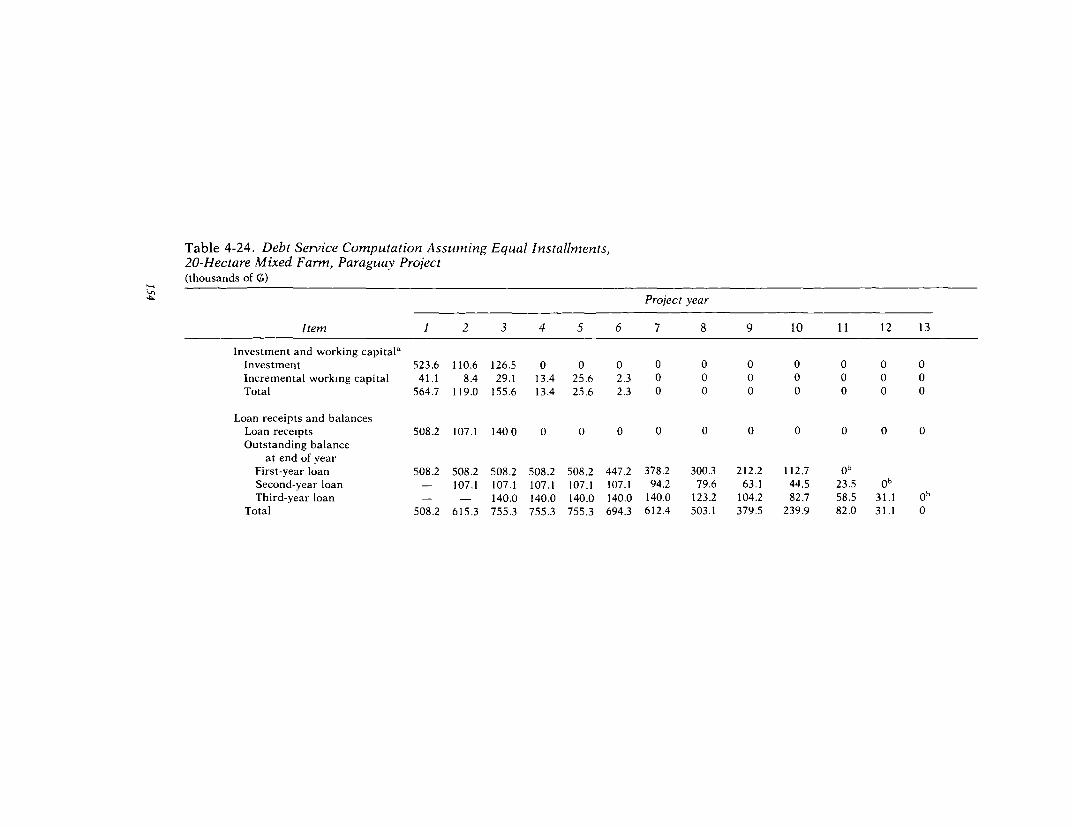
Table 4-24. Debt Service Computation Assuming Equal Installments,20-Hectare Mixed Farm, Paraguay Project(thousands of Q;)
Project year
Item 1 2 3 4 5 6 7 8 9 10 11 12 13
Investment and working capitalaInvestment 523.6 110.6 126.5 0 0 0 0 0 0 0 0 0 0Incremental working capital 41.1 8.4 29.1 13.4 25.6 2.3 0 0 0 0 0 0 0Total 564.7 119.0 155.6 13.4 25.6 2.3 0 0 0 0 0 0 0
Loan receipts and balancesLoan receipts 508.2 107.1 140 0 0 0 0 0 0 0 0 0 0 0Outstanding balance
at end of yearFirst-year loan 508.2 508.2 508.2 508.2 508.2 447.2 378.2 300.3 212.2 112.7 ob
Second-year loan - 107.1 107.1 107.1 107.1 107.1 94.2 79.6 63.1 44.5 23.5 ob
Third-year loan - - 140.0 140.0 140.0 140.0 140.0 123.2 104.2 82.7 58.5 31.1 ob
Total 508.2 615.3 755.3 755.3 755.3 694.3 612.4 503.1 379.5 239.9 82.0 31.1 0

Debt serviceFirst-year loan
Interest _ 66.1 66.1 66.1 66.1 66.1 58.1 49.2 39.0 27.6 14.7Repayment of principal - 0 0 0 0 61.0 69.0 77.9 88.1 99.5 112.4
Subtotal - 66.1 66.1 66.1 66.1 127.1 127.1 127.1 127.1 127.1 127.1Second-year loan
Interest - - 13.9 13.9 13.9 13.9 13.9 12.2 10.3 8.2 5.8 3.1Repayment of principal - - 0 0 0 0 12.9 14.6 16.5 18.6 21.0 23.7
Subtotal - - 13.9 13.9 13.9 13.9 26.8 26.8 26.8 26.8 26.8 26.8Third-year loan
Interest - - - 18.2 18.2 18.2 18.2 18.2 16.0 13.5 10.8 7.6 4.0Repayment of principal - - - 0 0 0 0 16.8 19.0 21.5 24.2 27.4 31.0
Subtotal - - - 18.2 18.2 18.2 18.2 35.0 35.0 35.0 35.0 35.0 35.0Total - 66.1 80.0 98.2 98.2 159.2 172.1 188.9 188.9 188.9 188.9 61.8 35.0
Net financing 508.2 41.0 60.0 ( 98.2) ( 98.2) (159.2) (172.1) (188.9) (188.9) (188.9) (188.9) (61.8) (35.0)
Source: Calculated from table 4-19. See text for a discussion of how the b. The total repayments of principal do not exactly equal the loan receiptscalculations were made. because of rounding. The outstanding balance, however, is shown as zero.
a. From table 4-19.
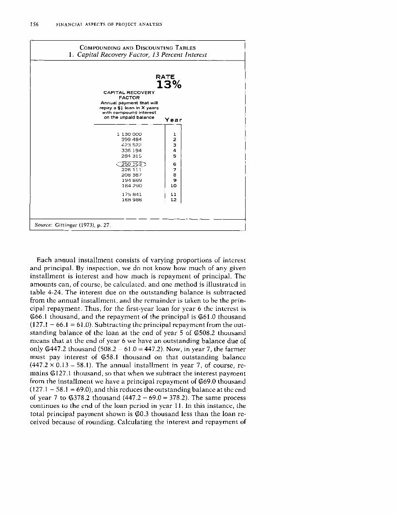
156 FINANCIAL ASPECTS OF PROJECT ANALYSIS
COMPOUNDING AND DISCOUNTING TABLES1. Capital Recovery Factor, 13 Percent Interest
RATE
13%CAPITAL RECOVERY
FACTORAnnual payment that willrepay a $1 loan in X yearswith compound intereston the unpaid balance Year
1 130 000 1599 484 2423 522 3336 194 4284 315 5
226 111 7208 387 8194 869 9184 290 10
175 841 11168 986 12
Source: Gittinger (1973), p. 27.
Each annual installment consists of varying proportions of interestand principal. By inspection, we do not know how much of any giveninstallment is interest and how much is repayment of principal. Theamounts can, of course, be calculated, and one method is illustrated intable 4-24. The interest due on the outstanding balance is subtractedfrom the annual installment, and the remainder is taken to be the prin-cipal repayment. Thus, for the first-year loan for year 6 'he interest is066.1 thousand, and the repayment of the principal is 061.0 thousand(127.1 - 66.1 = 61.0). Subtracting the principal repayment from the out-standing balance of the loan at the end of year 5 of 0508.2 thousandmeans that at the end of year 6 we have an outstanding balance due ofonly 0447.2 thousand (508.2 - 61.0 = 447.2). Now, in year 7, the farmermust pay interest of 058.1 thousand on that outstanding balance(447.2 x 0.13 = 58.1). The annual installment in year 7, of course, re-mains 0127.1 thousand, so that when we subtract the interest paymentfrom the installment we have a principal repayment of 069.0 thousand(127.1 - 58.1 = 69.0), and this reduces the outstanding balance at the endof year 7 to 0378.2 thousand (447.2 - 69.0 = 378.2). The same processcontinues to the end of the loan period in year 11. In this instance, thetotal principal payment shown is 00.3 thousand less than the loan re-ceived because of rounding. Calculating the interest and repayment of

FARM INVESTMENT ANALYSIS 157
Table 4-25. Debt Service Computation AssumingEqual Installments with Interest Capitalized,1-Hectare Planting, India Cashewnut Project(Rs)
Compounding factor Principal and interestYearof Amount of for I due at endloan loan (10.5 percent) of fifth year
1 783 1.490 902 1,1672 468 1.349 233 6313 1,482 1.221 025 1,8104 733 1.105 000 8105 338 1.000 000 338Total 3,804 4,756
Interest during sixth and seventh years = Rs4,756 x 0.105 = 499Combined annual installment of interest and principal repayment
due from eighth through thirteenth years =4,756 x 0.232 982 = 1,108
Source: Same as table 4-21. See text for a discussion of how the calculations were made.
principal year by year as done here is generally unnecessary; simplycalculating the equal annual installment using the capital recovery fac-tor ordinarily will suffice.
Equal installments with interest capitalized
In some loan transactions, the lender will agree to "capitalize" theinterest due during the grace period. This means that the borrower neednot pay any interest during the grace period; the interest due is, in effect,added to the principal of the loan (hence the term "capitalize"). When therepayment of principal begins, the amount borrowed plus the interestadded to the principal during the grace period is then repaid in a series ofequal installments.
We may illustrate how to calculate the interest payment and therepayment of principal by an example adapted from the Indian Cashew-nut Project (discussed earlier in connection with unit activity budgets).The credit computation for the India project is laid out in table 4-25. Afarmer is to be loaned Rs3,804, disbursed over five years, to establish astand of cashewnut trees. The loan term is for twelve years at 10.5 percentinterest with a six-year grace period. Interest due during the disburse-ment period in years 1 through 5 is added to the principal-that is,capitalized. Interest on the capitalized amount is to be paid in years 6and 7. Repayment of the principal plus capitalized interest is to be madein six equal annual installments beginning at the end of the eighth yearand ending at the completion of the thirteenth year.
For each year that the loan is being disbursed, the amount of thedisbursement is multiplied by the compounding factor for 1 for the

158 FINANCIAL ASPECTS OF PROJECT ANALYSIS
remaining length of the disbursement period to determine the amount ofprincipal and interest due on that disbursement at the end of the dis-bursement period. The compounding factor for I may be obtained fromGittinger (1973) or from a similar source, or it can be calculated using asimple electronic hand calculator (see chapter 10, the section "Calcula-tor Applications in Project Analysis"). For the disbursement made in year1, for example, the amount of principal and capitalized interest due bythe end of the fifth year is calculated by multiplying the principal re-ceived, Rs783, by 1.490 902, which is the compounding factor for I at 10.5percent interest for the number of years after the loan is disbursed untilthe end of the fifth year-in this case, four years. The result is a total dueof Rsl,167 (783 x 1.490 902 = 1,167). The amounts of principal and in-terest due on each disbursement at the end of the fifth year are thentotaled to determine the total principal and interest due at the end of thatyear. Interest is paid on that capitalized interest in years 6 and 7 in theamount of Rs499 (4,756 x 0.105 = 499). The annual installment neces-sary to pay the interest due and to repay the principal in six equalpayments is determined by taking the total value of Rs4,756, the loanoutstanding at the end of the fifth year including capitalized interest, andmultiplying it by 0.232 982, the capital recovery factor for six years at10.5 percent interest, to obtain the annual installment of Rsl,108thousand (4,756 x 0.232 982 = 1,108). (The capital recovery factor for sixyears at 10.5 percent interest was calculated by taking the reciprocal ofthe present worth of an annuity factor for six years at 10.5 percent. Seechapter 10, the section "Calculator Applications in Project Analysis," fora discussion of how to make the computation using a simple calculator.
Declining real burden of debt service
The examples of debt service calculation to this point have assumedthat debt service will be constant in real terms. Yet in most countrieslending terms to farmers call for repayment in nominal-that is,money-terms. Interest is stated at a given rate, and the nominal amountof principal repayment is agreed upon. If there were to be inflation,which would reduce the real value of money over time, the result wouldbe that farmers would have a declining real burden of debt service overthe life of the loan. If a farmer agrees to make a series of fixed annualinstallments to repay his loan, the real burden of that fixed installment isreduced by the extent the value of money declines. (Some countries indexloans so that the nominal amount the farmer pays increases with infla-tion to maintain the farmer's real debt burden.)
We have noted that it is common practice in project analysis to dealwith inflation by assuming that all prices will move by the same propor-tion. Thus, relative prices remain the same-or the analyst changes theprice he uses to reflect the change in relative value. Our calculations,then, are done at constant prices. This convention generally is appropri-ate for farm investment analysis, with one important exception-repay-

FARM INVESTMENT ANALYSIS 159
ment of credit in fixed money terms. When there is inflation, if our farmbudget shows the same amount of debt service to repay a loan each year,we in effect are assuming that the loan is indexed and that its real burdenwill remain the same relative to all other prices. The opposite, however,is often true-inflation raises the nominal prices of the goods and servicesthe farmer buys and sells, but the nominal amount of the debt burdenremains the same. Thus the real burden falls, and if our project accountsare cast in constant terms the debt service should be reduced to reflectthe changing value of the debt service payment relative to other prices.Such adjustments have been infrequent in project analysis to date, butwith continuing high inflation in many countries it is a reasonable ex-pectation that they will become more common.
An illustration of a farm budget that assumes a declining real burden ofdebt service, based on the farm budget for the Paraguay project used intable 4-19, was given in table 4-20. The debt service under this assump-tion is worked out on the basis of equal nominal annual installments intable 4-26. It is assumed that there will be constant inflation of 8 percentduring the period of the financing. The terms and conditions of thefinancing are the same as those used in the example of equal annualinstallments in table 4-24-the loan is for ten years at 13 percent interest,with a four-year grace during which interest is paid and with six equalannual installments of interest and repayment of principal thereafter.
The loan receipts in real terms are taken from table 4-24. They are, infact, stated in constant terms in guaranis of project year 1. It is assumedthat the farmer will continue the real investment program laid out in thefarm budget in constant terms of table 4-18, so that in nominal terms thesecond- and third-year loans will increase by the amount of the inflation.To calculate the nominal amounts, the real value is multiplied by thecompounding factor for I for the number of years after project year 1,which is the base year for the computation. [The compounding factor for1 may be obtained from Gittinger (1973) or some similar source.] Thenominal amount of the second-year loan, then, would be its real value of0107.1 thousand multiplied by 1.080 000, the compounding factor for 1for 8 percent (the assumed inflation rate) for one year, and this gives theresult of 0115.7 thousand (107.1 x 1.080 000= 115.7). The nominalamount of the third-year loan is the real value of 0140.0 multiplied by1.166 400, the compounding factor for 1 for two years, and this gives theresult of 0163.3 thousand (140.0 x 1.166 400 = 163.3). For this and allother calculations where the compounding factor for 1 is used, repeatedmultiplications or divisions may be used (140.0 x 1.08 x 1.08 = 163.3). Ifa calculator is available that computes powers directly, the nominalvalue of the third-year loan may be simply determined by raising I plusthe rate of inflation to the power of the number of years after the basedate (140.0 x 1.082= 163.3).
The calculation of the debt service in nominal terms is given forcomparison with the nominal calculation in table 4-24 and with thecalculation in real terms later in table 4-26. The nominal debt service is

Table 4-26. Debt Service Computation Assuming Equal Installments and Declining Real Burdenof Debt Service, 20-Hectare Mixed Farm, Paraguay Project(thousands of G;)
Project year
Item 1 2 3 4 5 6 7 8 9 10 11 12 13
Loan receiptsReal termsa 508 2 107.1 140.0 0 0 0 0 0 0 0 0 0 0
Nominal terms 508.2 115.7 163.3 0 0 0 0 0 0 0 0 0 0
Debt serviceNominal terms
First-year loan - 66.1 66.1 66.1 66.1 127.1 127.1 127.1 127.1 127.1 127.1 - -
Second-year loan - - 15.0 15.0 15.0 15.0 28.9 28.9 28.9 28.9 28.9 28.9 -
Third-year loan - - - 21.2 2; 2 21.2 21.2 40.8 40.8 40.8 40.8 40.8 40.8
Total - 66.1 81.1 102.3 102.3 163.3 177.2 196.8 196.8 196.8 196.8 69.7 40.8
Net financing 508 2 49.6 82.2 (102 3) (102.3) (163.3) (177.2) (196.8) (196.8) (196.8) (196.8) (69.7) (40.8)
Real termsbFirst-year loan - 61.2 56.7' 52.5c 48 6 86.5 80.1 74.2 68.7 63.6 58.9
Second-year loan - - 12.9 11.9 O1.0c 10.2 18.2 16.9 15.6 14.4c 13.3c 12.3c -
Third-year loan - - - 16.9 15.6 14.4 13.3' 23.8 22.0c 20.4 18.9 17.5 16.2
Total - 61.2 69.6 81.3 75.2 111.1 111.6 114.9 106.3 98.4 91.1 29.8 16.2
Net financing 508.2 45.9 70.4 ( 81.3) ( 75.2) (111.1) (111.6) (114 9) (106.3) ( 98.4) ( 91.1) (29.8) (16.2)
Source: Calculated from tables 4-19 and 4-24. See text for a discussion of compounding factor for I for two years, 1.166, to obtain the interest payment
how the calculations were made. of t12.9 thousand (115.7 x 0.13 - 1.166 = 12.9). For the first annual install-
a. From table 4-24. ment of combined interest and principal repayment for the second-year loan,
b. Calculated by dividing each entry in the line, except for the first interest the nominal amount of the loan of 115.7 thousand is multiplied by the capital
installment and the first installment of combined interest and principal repay- recovery factor for six years at 13 percent, 0.250 153, and then divided by the
ment, by 1.08. These exceptions are determined by multiplying the nominal compounding factor for I for six years, 1.587, to obtain the payment of q; 18.2
amount of the loan by the interest rate or the capital recovery factor and then thousand (115.7 x 0.250 153 - 1.587 = 18.2).
dividing by the compounding factor for 1 for 8 percent (or 1.08") for the c. Calculated as explained in note b; this calculation introduces a slight
number of years after the first year of the project. Thus, for the first interest rounding error. Direct calculation using the formulas in the text obtains a
payment for the second-year loan, the nominal amount of the loan of Qil 15.7 slightly different result.
thousand is multiplied by the interest of 13 percent and then divided by the

FARM INVESTMENT ANALYSIS 161
calculated in the same manner as the computations in table 4-24 but isbased on the nominal amounts of the loan receipts. Thus, for the second-year loan the nominal interest during the grace period would be thenominal value of the loan receipt of 01 15.7 thousand multiplied by theinterest rate of 13 percent, and this gives an interest payment of 015.0thousand (115.7 x 0.13 = 15.0). The equal annual installment would bethe nominal value of the loan of 0115.7 thousand multiplied by 0.250153, the capital recovery factor for six years at 13 percent, and this givesan installment of 028.9 (115.7 x 0.250 153 = 28.9).
To calculate the debt service in real terms, the nominal amounts mustbe reduced by the extent of inflation since the loan was made. To do this,the nominal amount is divided by the compounding factor for 1 for thenumber of years involved. For the first-year loan, the receipt is 0508.2thousand, and the nominal payment due at the end of year 2 at a 13percent interest rate is 066.1 thousand (508.2 x 0.13 = 66.1). Since infla-tion is assumed to be 8 percent, the real burden is reduced between theloan receipt at the end of year 1 and the first interest payment at the endof year 2; this reduction makes the real burden of the first interestpayment in guaranis of project year 1 only 061.2 thousand (66.1+ 1.08 = 61.2). In year 3, the interest in real terms is again reduced by the
amount of the inflation, to 056.7 thousand (61.2 . 1.08 = 56.7). The in-terest in years 4 and 5 is calculated in a similar manner.
Repayment of principal combined with interest on the remainingoutstanding balance begins in year 6. The equal annual installment innominal terms that the farmer would pay from years 6 through 11 isdetermined by multiplying the amount of the loan received, 0508.2thousand, by the capital recovery factor for six years at 13 percent, 0.250153. The result is a nominal payment of 0127.1 thousand (508.2 x 0.250153 = 127.1). Since this is in nominal terms, the real burden is reduced byfive years of inflation between the end of year 1, when the loan is received,and the end of year 6, when the first annual installment of interest andprincipal repayment is made. To do this, the nominal payment of 0 127.1thousand is divided by the compounding factor for 1 for 8 percent for fiveyears to obtain the real burden of the payment at the end of year 6, 086.5thousand (127.1 . 1.469 328 = 86.5). In year 7 the real burden is againreduced by the amount of the inflation, and this gives a real burden of080.1 thousand (86.5 . 1.08 = 80.1). The same process is continuedthrough the remaining life of the loan.
For the second-year loan, the debt service is again calculated on thebasis of the nominal value of the loan, 0115.7 thousand. The nominalinterest due during the four-year grace period at the rate of 13 percent,therefore, is 015.0 thousand (115.7 x 0.13 = 15.0). This payment is due,however, in year 3, or two years after the base of the constant value,which is stated in year-1 guaranis. Hence, the nominal value of theinterest payment must be reduced by the amount of inflation in bothyears 2 and 3 by dividing it by the compounding factor for 1 for two yearsto obtain the real value at the end of year 3, which is 012.9 thousand

162 FINANCIAL ASPECTS OF PROJECT ANALYSIS
(15.0 -- 1.166400 = 12.9). The real value of the interest payment in year 4may be obtained by dividing the interest payment made in year 3 by 1plus the inflation rate stated in decimal terms, and this gives 01 1.9thousand (12.9 . 1.08 = 11.9). The nominal value of the equal annualinstallment from years 7 through 12 is obtained by multiplying thenominal value of the second-year loan of 01 15.7 thousand by 0.250 153,the capital recovery factor for six years at 13 percent; the result is l28.9thousand. Since this amount is due at the end of the seventh project year,or six years after the base in project year 1, it is divided by the compound-ing factor for 1 for six years to obtain the real value of 0i18.2(115.7 x 0.250 153÷ 1.586 874 = 18.2). The real burden of the next in-stallment in year 8 is obtained by dividing the year 7 payment of 018.2thousand by 1.08; this yields 016.9 thousand (18.2 . 1.08 = 16.9). Thesame process is continued through the life of the loan.
Determining the real burden of each payment is more rapidly andaccurately accomplished if an algebraic formula is used instead of theiterative process outlined here. The interest during the grace period maybe determined as:
L(1R+Y' -(1 +f) M
the real burden of the annual installment of combined interest andprincipal may be determined as:
R*m _ L(1 + f)n - 'F(1 + f)M
in both equations,
Rm = real burden of debt service in project year m during graceperiod
R*m = real burden of debt service in project year m during period ofannual installment of combined interest and repayment ofprincipal
n = project year in which loan is receivedm = project year in which debt service is madeL = real value of loan receiptF = capital recovery factorr = rate of interest paid on loanf = rate of inflation.
If a calculator that determines powers directly is not available, thecompounding factor for I for the appropriate rate and number of yearsmay be used in place of the expressions (1 + f)n - ' and (1 + f) - '.
Although we have by no means given examples of all possible loanterms in this section, the debt service for most other loan terms may bereadily calculated following these illustrations.

FARM INVESTMENT ANALYSIS 163
Appendix. Herd Projections
A basic element in the analysis of agricultural projects that involve alivestock component is a projection of the number of animals. For smallanimals with a generation interval within the accounting period-forexample, poultry-the projections can be done simply by estimating thenumber of animals that can be maintained with the feed and facilitiesavailable. This usually is also the approach for hogs. But for largeranimals that take more than one accounting period to mature-includ-ing dairy and beef cattle, sheep, and goats-the projections are usuallybased on herd buildups that reflect the number of breeding animals, thenumber of animals born, mortality, and sales. A pattern herd projectionis given in table 4-27; it is based on the Paraguay example and is compati-ble with the accounting convention recommended for farm budgets inthis book. A herd productivity computation is given in table 4-28.Whether estimated directly or through the use of a more elaborate herdprojection, the number of animals forecast is then priced and the valueincorporated in the farm budget as was illustrated in the Paraguayexample. [This appendix draws heavily from materials especially pre-pared by Meyn, Gittinger, and Schaefer-Kehnert (1980) and Schaefer-Kehnert (198 la)].
In the text of this chapter (the subsection "Farm Production. Live-stock"), we noted that the purpose of a herd projection is to apply to aherd at the beginning of a project technical coefficients that are estimatesof the improvements in management, animal health, and nutrition theproject investment will make possible. The herd projection allows esti-mates of future feed requirements, handling facilities, investments, andthe productivity of the herd. The herd development is continued until-through natural increase, purchases, or reduced sales-the herd hasreached a level at which it can make best use of the available resources.
In the same subsection of the text we also noted that, for small farmsinvolving dairy or beef cattle (and to some extent sheep and goats), theproblem of divisibility (the reporting of fractional animals) must beresolved. The most satisfactory method of doing this is to take a group offarms-often 100-and to project the herd for all the farms in the group.All calculations in the projections can then be rounded to the nearestwhole animal. This avoids having fractional animals in the herd projec-tion, which happens when the technical coefficients are applied to thenumber of animals in a small herd. The values for purchases and sales forthe full 100-farm group are then divided by 100 and entered in the farmbudget for the individual farm. In effect, this assumes that on the averagea farm will have a given level of purchases and sales. Although thisconvention is not fully satisfactory, it is better than trying to projectherds on the basis of probability or carrying fractional animals in theprojection until they aggregate to a whole animal.
Herd projections generally are done by someone with a considerable

164 FINANCIAL ASPECTS OF PROJECT ANALYSIS
knowledge of livestock production because these projections depend onjudgments about feed availability, management improvement, and thelike. Thus, most agricultural project analysts would turn to a livestockspecialist for assistance with a herd projection, just as they would turn toother agricultural specialists for assistance with such things as cropyields or irrigation construction costs.
We will illustrate the methodology of herd projections with the exam-ple of the Paraguay project we have been following in this chapter. This isfor a beef production activity on a 20-hectare mixed farm, but with ratherminor adaptations it can be used for a dairy herd or, with somewhatmore adaptation, for sheep and goats.
Terminology and definitions
Livestock specialists use a group of special terms that may not befamiliar to all agricultural project analysts. A breeding cow is, of course,the mature female of the species that has borne at least one calf; the maleis the bull. A calf (plural, calves) is the young animal; its age in theseprojections is one year and less. Heifers are young females that are olderthan calves but younger than a predetermined age (in this case, threeyears) and that have not yet borne calves. Steers are castrated maleanimals. Culled animals are those taken from the herd because they donot meet performance standards.
Carrying capacity refers to the ability of an area of pasture to supportanimals; it is generally expresEed in terms of animal units, a standardmeasurement of feed. By expressing carrying capacity in animal units, asingle measurement for the pasture requirements of the herd is obtained.The standard animal, or one animal unit, in herd projections for cattle isusually a cow of average size in the reference area.
Computational conventions
A group of simplifying conventions makes calculation of the herdprojection less complex and allows it to fit with the accounting conven-tion used for the rest of the farm investment analysis. Analysts vary in thedetails of the conventions they apply, but the ones we will discuss here,which are used in tables 4-11 and 4-27, are fairly representative, areconsistent, and are amenable to computation by hand with a simplecalculator.
All calculations are rounded to the nearest whole animal. Stock takingfor the analysis occurs at the end of the year. Purchases enter the herd atthe end of the accounting year, and sales from the herd also occur at theend of the accounting year. Adult mortality is calculated on the basis ofthe number of animals present at the beginning of the year. For calves,mortality is deducted from the number of calves born during the courseof the year. Internal transfers of young animals are accomplished bycarrying forward the end-of-year closing stock figure to the opening stockfigure of the next higher age category at the beginning of the next year.Transfers of heifers 2-3 years old are added to the number of breeding

FARM INVESTMENT ANALYSIS 165
cows at the end of the year, the sum being the closing stock of breedingcows for that year. For bulls and work oxen, the previous end-of-yearfigures serve as beginning-of-year figures in the following year. Thenumber of bulls in the Paraguay example is taken to be one for each farm,or 100 bulls in the 1 00-farm herd. The number of bulls required, however,would usually be a function of the number of breeding cows in the herd atthe beginning of the year. Additional bulls needed, including thoseneeded for purchased heifers brought into the herd, are assumed to bepurchased at the end of the year. There would usually be three to fourbulls for 100 breeding cows. For the purpose of the projection, male andfemale calves are accounted for separately, and the numbers of each aredetermined by multiplying the number of breeding cows at the begin-ning of the year by half the calving rate. Treating male and female calvesseparately permits the analyst to apply different technical coefficients tomale and female calves, if that reflects reality (the case for calf mortalityin East Africa, for example), or to make assumptions that male andfemale calves will be treated differently (the case in dairy operationswhere male calves may be sold soon after birth). Culling rates are appliedto the number of animals at the beginning of the year.
Since herd projection computations can become quite complex, it isimportant to have good worksheets. A pattern herd projection worksheetthat uses data from the Paraguay example is shown in table 4-27. Thispattern can rather easily be adapted to the conditions and assumptionsof different projects, which vary so widely as to make it impractical tohave a standardized worksheet. As these adaptations are made, severalprinciples should be kept in mind so that the worksheet will remaincompatible with the accounting convention recommended for farmbudgets, Year 1 is reserved for investment (which may extend over morethan one year). Production in year I may be reduced by the investment-by plowing grassland to establish improved pasture, for example. In-cremental production begins no earlier than the beginning of year 2; itmay begin later if investment takes longer. All purchases and sales, aswell as transfers of animals to another category, take place at the end ofeach year. Thus, purchases that are part of the investment take place atthe end of year 1. The first sales generated through incremental produc-tion can occur no earlier than the end of year 2. Heifers retained asbreeding cows are transferred at the end of each year. Using brackets toinsert the technical coefficients, and boxes to indicate the elements of thepreliminary closing stock, are format devices that greatly reduce thelikelihood of error when using the worksheets.
Technical coefficients
The herd projection is built up by applying the technical coefficients tothe initial herd until a herd size is reached that just consumes theincreased feed to be made available or until some other predeterminedlimit, such as the size of handling facilities and the like, is reached. Thetechnical coefficients come from field observation and statistics collectedby government services as the project is being prepared.

166 FINANCIAL ASPECTS OF PROJECT ANALYSIS
For the Paraguay example, the technical coefficients without the proj-ect were determined to be those given in the last part of table 4-27. Ingeneral, these improve over the life of the project, in reflection of theanalyst's assumption about the effects on the number of animals ofproject investment and improved management by the farmer. In a herdprojection, particular attention to the underlying biological facts mustbe paid. For example, assume that 30 percent of the bulls in a herd will bereplaced with bulls of an improved breed at the end of year 1. Suppose inaddition that the age of first calving for heifers in the herd is three to fouryears. Not until year 5 can introducing better bulls have any effect onherd production. At that time, 30 percent of the steers three to four yearsold will be heavier, and 30 percent of the heifers giving birth to calveswill produce more milk. Very often these facts are neglected; the result isan overoptimistic projection that field results cannot meet.
CALVING RATE. The calving rate is the proportion of breeding cows thatbear live calves during the year. It is applied to the number of breedingcows in the herd at the beginning of the year. In the pattern worksheet,the number of male and female calves is determined separately by divid-ing the calving rate in half. In the Paraguay example the calving rate isexpected to improve from 70 percent at the beginning of the project to 75percent as a result of improved management. The calving rate of 80percent during year 3 is the result of purchasing in-calf heifers, whichincreases the calving rate. Calving rates range from about 50 percent oreven less in pastoral herds in areas with one long dry season a year toabout 90 percent in well-managed herds in areas with high potential.
CALF MORTALITY. The calf mortality is the proportion of live calves bornduring the year that do not survive to the end of the year. It applies to thenumber of calves born during the year. In the Paraguay example, it isassumed that improved management will reduce the calf mortality from10 percent without the project to 5 percent by project year 4. Calfmortality ranges from 40 percent in cattle herds kept under extremenutritional and climatic stress to less than 3 percent in well-managedbeef herds in a favorable environment. Calf losses of 10 percent arecommon even in well-managed dairy herds.
ADULT MORTALITY. The adult mortality is the proportion of animalsolder than one year that are lost during the year. It is applied to thenumber of adult animals in each class at the beginning of the year. It iscustomary to apply the adult mortality rate to all animals above one yearold, although losses somewhat higher than average may be expectedamong first-calf heifers and older cows. In the Paraguay project, adultmortality is already low at 3 percent at the beginning of the project anddeclines only slightly to 2 percent from year 3 of the project because ofbetter husbandry. Adult mortality ranges from 10 percent to about 2percent under practical conditions in developing countries.
CULLING RATE-BULLS. The culling rate for bulls is the proportion ofbulls removed from the herd each year because they fail to meet the

FARM INVESTMENT ANALYSIS 167
performance standards or reach a predetermined culling age. It is ap-plied to the number of bulls in the herd at the beginning of the year. In theParaguay project, the culling rate for bulls would increase slightly from15 percent to 18 percent. This reflects a decrease in the productive life ofthe bulls from about 5.6 years assuming a 3 percent mortality rate[1 . (0.15 + 0.03) = 5.6] to about 5.0 years assuming a 2 percent mortal-ity rate [1 -. (0.18 + 0.02) = 5.01. The productive life of a breeding bullcannot be much longer than six years; usually it is two to eight years fortemperate-zone cattle and three to nine years for zebu cattle. Whengenetic improvement is an important part of the management system,farmers will change bulls more frequently than required by the biologi-cal utility of the bull.
CULLING RATE-COWS. The culling rate for cows is the proportion ofbreeding cows removed from the herd each year because they do notmeet the performance standards. It is applied to the total number ofbreeding cows at the beginning of the year. In the Paraguay example, theculling rate rises from 12 percent at the beginning of the project to 15percent in years 2 and 3, a result of an attempt to improve the perfor-mance standard of the breeding cows. It then drops slightly to 14 percent.At a 14 percent culling rate and a 2 percent mortality rate, the averageproductive life of a breeding cow would be about 6.2 years[1 - (0.14 + 0.02) = 6.2]. If the age of first calving is taken to be 4 years,this implies that the cows would normally leave the herd at about 10.2years of age (6.2 + 4 = 10.2). The productive life of cows in a breedingherd ranges from three years in intensive dairy herds to about eight yearsin beef herds, equivalent to a culling rate of 33 percent and 12 percentrespectively, excluding mortality.
CULLING RATE-HEIFERS. The culling rate for heifers is the proportion ofheifers that are unsuitable for breeding. It is applied to the number ofheifers ready for service at the beginning of the year. In the Paraguayexample, heifers two to three years old are considered ready for service,but'heifers of one to two years are assumed not to be ready and so are notculled. In this example, the culling rate for heifers rises from 5 percentwithout the project to 10 percent beginning in year 2. The higher cullingreflects tighter performance standards for breeding cows. In most breed-ing herds, from 5 to 10 percent of the heifers would be expected to beunsuitable for breeding.
CULLING RATE-WORK OXEN. The culling rate for oxen is the proportionof the oxen removed each year because they do not meet the performancestandards. In the Paraguay project, the culling rate is assumed to be 16percent, reflecting an average working life of some 6.2 years for oxen,about average in most parts of the world (1 . 0.16 = 6.2).
RATIO OF BULLS TO BREEDING FEMALES. The percentage of bulls in rela-tion to breeding cows is applied to the number of breeding cows in theherd at the beginning of the year. If in-calf heifers are purchased, addi-
(Text resumes on p. 174.)

168 FINANCIAL ASPECTS OF PROJECT ANALYSIS
Table 4-27. Herd Projection Worksheet, 100 20-Hectare Mtxed Farms,Paraguay Project(head)
Wtthout development Development year
Stable 1,000- 100-farmItem cow herd herd 1 2 3
Breeding bulls Livestock classOpening stock .. 100 -- 100 ...100 ---100 ---100- Deaths[% - 3 [ 3] -- 3 [3] -- 3 [ 3] -- 3 [ 3] -- 2 [2]-Culls [%b- 15[15] - 15[15] - 30 [30] -- 17 [17]1 - 18[18]
+ Purchases forexisting herd -+-- 18 -±-- 18 . .. 33 - --- 0 + 20
Subtotal [%]C -T7 [-] F=- 00 ool [-] I=- 1007 [-] F=7100 [- F] -i-o [-+ Purchases for
purchased
heifers -± --- 0 + --- 0 + --- 0 + --- 0 -+ --- 0Closing stock = 0 100 00oo 100 to10 10
Breeding cowsOpening stock 1lpOO-- 500 --500 -- 55- 800
-Deaths [%]a 30 [ 3] .-.. 15 [ 3] - 15 [ 3] - 20 [ 3 1 6 [ 2]-Culls [%]d ~~~~~-120- [12]------- ---8 [15 -- 20 [15
- CUIS [ ]d ---120 [21 ----60 [12] - __60 [12) 8 [510 [5Subtotal F 86 = 425 ~ F=-451 F= 537- = -
+ Heifertransfers + --150 -+-- 75 + _230 + --263 ± -136
Closing stock =1,000 =500 _ 655 =800 -- 800
Female calvesBirths [% ~350 [35] 15 [35] 15 [35] 246 [37.5] 320 [40]- Deaths -[-----35 [10] - ---- 8 [10] - --- 8 [10] --- 25 [10]- [_6 8]
Closing stock F 3 5 = 1577 F= 157 F-22 fl F-294
Heifers 1-2 yearsOpening stock -3 5 -1 7 -- 57 --1 7--2 1
~Deaths[% - 9 [3]--5 [3]- 5 [3]- 5 [3]--4 [2]
Closing stock F=-- 7 = 152~ J=121 F= T52~ =-17
Heifers 2-3 yearsOpening s tock 306 152 152 152 152- Deaths[%- 9 [ 3] . .... 5 [3] .--... 5 [ 3] .--... 5 [ 3] -- 3 [2]- Culls [%]5 - ---- S [ 5] ---- 8 [ 5]-.... 8 [ 5] ---- 5 [10]I ----- 15 [10]
Subtotal =2-82 F= 139~ F= 139-1 F-- ~ F--
- Sales ___132 .- .. 64 - ---- 0 - ---- 0 ----- 0-I Purchases + --- 0 +-----0 -±-- 91 +-I+ 2Transfer to cows 150 = 75 230 =263 =136
Male calvesBirths [%]1 350 [35] 7 [35] I7 [35] 246 [37.5] .. , [40]- Deaths [%] .-.. 35 [10] -- 8 [10] - 18 [10] -- 5 [10 I .--.. 6 8]
Closing stock F=3--51 F=- 57-1 =7 -71 F=1-2- i F -9-4
Steers 1-2 years
Opening stock --315 ---157 1--I57 ---I57--22I- Deaths[-%------
9[3] ------ 5 [3] - ----- 5 [3] .--... 5 [3] ------ 4 [2]
Subtotal F=- 306~ =-152l F--1-1 F= i1l-2 217l1
+ Purchases ±-0 +-0 + 0 + 0 + 0
Closing stock .. 306 =--- 2 .. 152 --- 1-52 -- 21-7

FARM INVESTMENT ANAIYSIS 169
Development year Full development
Stable 1,000-4 5 6 Years 7-20 cow herd
Livestock class100 100 100 100 100
-2 [2] -. 2[ 2] - 2 2 - [] 2 -- [ ] -- 2[ 2- 8 [18 ] - 18 [18 ] -- 18 [18 ] -- [18 -- 18 [18 ]- 18 [18]
+ 20 + 20 + 20 + + 20 +20
- -- [] = 00 F] [] = [] - 0 [] = [-]- --- l
+ o + o + o - + - + -
- 100 = 100 = 100 = = 100 = 100
800 800 800 800 ilooo
-- 6 2] -- 6[ 2] -- 6[ 2 -- [ 2 -- 6 [ 2 ] -- 20 [ 2]
-- 112 [14 ] -- 12 [14 ] -- 1 2 [14 -- [14 --- 12 [14 ] -40 [14
-= 67 2 = 672 67= 82
+-128 + 128 +128 + + 128 + 160
800 = 800 = 800 = = 800 =1,00.0
300 [37.5] 300 [37.5] 30Q [37.5] [37.5] 300 [37.5] 37s [37.5]
- 1-5 [5 ] - -- [ s ] - -- [ s ] - - [ ] - 15 [ s ] - 9 [5]
F= 2851 F= 28s F= 28- -2 = .
294 285 285 285 356-6[2]--6 [2]--6 [ ]-- [2] ---- 6 [2 -- - []
-2 =- = --279= -- 279 349
217 28 279 279 349-- 4 [ 2]- 2 ]- [2 -- [ 2 ] - 6 2 ]- 7 [2 ]-- 22 [0 ] -- 29 [10 ] - 28 [10 [10 ] - 28 [10 ] - 35 [10
.l9 11 = 2531 F= 2451 [ 245 t F= 3077- ----- 3 --- - ------ -=----
- 63 �� - 11 - -- 1-7-- 147+ + O+ 0 + + 0 + -
= 128 = 128 = 128 --------- = 128 = 160
300 [37.5] 300 [37.5] 300 [37.5] [37.5] 300 [37 5] 375 [37.5][ 5 ] - [ 5 ] ~~~~~~~------ ---------.------- - ---- --X [ - i [5]- .... [5]- 5 [ 5]- - [5]- S [5]--19 [ 5]
2I8 ==- 28S =- 2 =8-585 = 3-61
294 285 285 285 356
-- [ 2] --- [2] .--- ] -- [2]- 6 [2]- [2]
1=-2881 1= 2791 2F=2 79=- F= 3491I ~ ~ ~ ~ ~ ~ ~ ~ ~ I - --- .- --- - ------ ,
+-0 + + 0 + +288 = 279 = 279 = = 279 = 349
(Table continies on the following pages.)

170 FINANCIAL ASPECTS OF PROJECT ANALYSIS
Table 4-27 (continued)
Without development Development year
Stable 1,000- 100-farmItem cow herd herd 1 2 3
Livestock classSteers 2-3 years
Opening stock 306 152 152 152 152- Deaths [%. - 9 3] -- 5 [ 3] -- 5 [ 3] -- 5 [ 3 ] -- 3 [ 2]
Closing stock |= 2977 = 1471 F-T 147| = 471 49
Steers 3-4 yearsOpening stock 297 -47 147 147 I47- Deaths [%]D -_9 [ 3] -- 4 [ 3] _ 4 3] -- 4 3 ] -- 3 1 2]Sales = 288 = 143 143 = 143 = 144
Work oxenOpening stock - 0 0 200 200- Deaths [%] ---. 1 3] - P 0. 3] -. [ 3] -- 6. 3 ] - 4 L 2]
Culls [%] - [] 0 [- ] - 0 0] - 32 [16] - 32 [16]+ Purchases for
existing herd +- - + 0 + 200 + 38 + 36
Closing stock = | 2001 = 200
Herd totalsTotal herd stock
Opening 21639 i,365 1,365 1,720 1,993
Prelim. closing | , 77 I | 1I4297| | _1 29 | 186!2 | 2.269|
Over(under)-stocking - 169 ( 91) ( 308) ( 351)Balancing sales
Heifers 2-3 years - 132 -- 64 - 0 - 0 -- 0Balancing purchases
Heifers 2-3 years +- 0 +- 0 + 91 + 131 + 2Bulls for above + - + 0 + 0 + 0 + 0Steers 1-2 years +- 0 + 0 +- 0 0 -- 0
Actual closing =2,639 =1,365 =1,720 =1,993 =2 271Carrying capacity
(end of year)' 1,260 1,720 2 170 2,620
Herd growthHerd composition
(opening stock)Bulls 100 100 100 00Breeding cows 500 500 655 800Heifers 1-2 years - 157 -57 -57 221Heifers 2-3 years 152 152 ---- 152 -52Steers 1-2 years 157 157 157 221Steers 2-3 years 2 152 152 152Steers 3-4 years 147 147 147 147Work oxen - 0 -20 200Total (animal units) 1,365 1,365 1,720 1,993
Carrying capacity(beginning of year)' 1Ž260 1-260 1,720 -7
Purchases
Bulls 18 33 20 20Heifers 2-3 years 0 91 1 2Steers 1-2 years 0 0 P 0Work oxen 0 200 38 36Total 18 324 189 58

FARM INVESTMENT ANALYSIS 171
Development year Full developmient
Stable 1,000-4 5 6 Years 7-20 cow herd
Livestock class217 288 279 279 349
4 2 ] 6 2] -- 6 [2] - [2] - 6 [2] - [2
| = ?73 F= 282 F- 273 1 | 2731 = 342
213 282 273 3423 [2] - 4 [2 ] -- 6 [2 ] -- [2 ] -- 5 2 ] -- 71 2]
= 146 = 209 = 276 = = 268 = 335
--- 200 200 200 200 200242] . 4... 2] -4-2 - ---[2]- 42 - 4 2]
2 [16 ] - 32 [16 3 -- 2 [16 ] - - [16 ] - 32 [16 ] - 32 [16
+ 36 + 36 + 36 + + 36 + 36
- 2-00 1 F=2 2001 1= 200 - 2001
Herd totals
2,271 2,459 2,510 2,501 3052
F 2,522 rFw 2,35 F 2,6181 F 2,618~ F 3, 199
( 98) 15 2) (-2)
63 - 125 - 117 - - 117 - 147
± 0 + 0 + 0 + + 0 + 0
+ - + ----- 0+ - - - - -0 + 0
+ --- 0 + --- 0 + --- 0 + ---- + 0 + --- 0=2,459 =2,510 =2-50i - =----- 2,5 3,052
___2__ 2 620 2 620_ 2___ _6_!_._
Herd growth
00 100 100 100
.S9 .S0. .S9300 800 800 800294 285 285 285217 288 279 279
294 5 285 285217 288 --29 279
-13 28 7200 200 200 200
2M271 2 2,510 -- 5--
2A620 2A620 2!620 _____2!620
20 20 20 20
0 -- --0 --- ---- ---0 -- ---0 -- -- ---0 - ----- ---0- ----
36 36 -36 3656(b sp56 56
(Table continues on the following pages.)

172 FINANCIAL ASPECTS OF PROJECT ANALYSIS
Table 4-27 (continued)
Without development Development year
Stable 1,000- 100-farnItem cowv herd herd 1 2 3
Hlerd Growth
SalesCulled bulls 15 30 17 I8Culled cows 60 60 98 120Culled heifers 8 8 15 15
Surplus heifers 2-3years 64 0 0 0
Steers 1-2 vears 0 0 0 0Steers 3-4 years 143 ---- 3 144Culled work oxen - 0 32 32Total 290 241 305 329
Technical coefficients (percenit)
Calving rate 70 70 75' 80'Calf mortality 10 10 10 8Adult mortality 3 3 3 2Culling rate, bulls 15 30 17 18Culling rate, cows 12 12 15 15Culling rate, heifers 5 5 10 10Culling rate, work
oxen - 0 16 16Bulls/breeding
femalesk _ _Carrying capacity
(per hectare,end of year)' 1.2 1 6 2 1 2 5
Without-development
area carrying capacitY 1,260 - 100 1,160_ _ _ _ _ _ _ _ _ _ _ _ _ _ _ _ _ _ _ _ _ _ _ _ - Z 0 4 5 7
Witliout-developinent pastuire 2,639 - 100 2,539requirement of stable
1,000-cowv herd + followers
Note: Brackets indicate technical coefficients; parentheses indicate negative numbers; boxes indicateelements of preliminary closing stock. The blank column before the columns under the heading "fulldevelopment" is included because the analyst will not know in advance just how many years it will taketo achieve full development. The worksheet should include a generous number of columns under theheading "development year" even though at the end of the herd computation some of these will beunused.
Source: Same as table 4-11.a. Adult mortality rate. e. Onc-half of calving rate.b. Culling rate of bulls. f. Calf mortality rate.c. Bulls/breeding females rate. g. Culling rate of heifers.d. Culling rate of cows. h Culling rate for work oxen.

FARM INVESTMENT ANALYSIS 173
Development year Full development
Stable 1,000-4 5 6 Years 7-20 cow herd
Herd Growvth
----18 - --18 - --18 ----- ---18112 ---- 2 ---1 2 2 --- -22 29 28 28
-63 125 117 117
146 209 276 268---- ~~~3 -- -- ----- -- ---- -----32 32 32 32
393 525 583 575
Technical coefficients (percent)
75 75 75 75 755 5 5 5 5 -----2 2 2 2 2
18 18 18 18 1814 14 14 14 1410 10 10 10 10
16 16 16 16 16
2.5 2.5 25 2.5 2 5
With-developmentarea cartytng capacrty 2,620 - 100 - 200 2,320
With-development pasture 3,052 - 100 - 200 2,752requirement of stable
1,000-cow herd + follouvers
i. In animal units. The carrying capacity at the beginning of the year is determined by multiplying theanimal units per farm at the end of the previous year given in table 4-10 by the 100 farms in the model.Similarly, the carrying capacity at the end of the year is determined by multiplying the animal units perfarm at the end of the year given in table 4-10 by the 100 farms in the model. The carrying capacity perhectare at the end of the year is determined by dividing the animal units per farm by the 10.5 hectares ofpasture on each farm; it is thus a weighted average of natural and improved pasture.
j. Represents a weighted average between the calving rate of breeding cows in the existing herd,which is 70 percent, and that of purchased bred heifers, which is nearly 100 percent.
k. Note that in this project a minimum of onebull perfarm is assumed,ora minimum of lOObulls on100 farms. The number of bulls per 100 breeding females would usually be three to four for all years.

174 FINANCIAL ASPECTS OF PROJECT ANALYSIS
tional bulls will be needed; the number is determined by multiplying thenumber of heifers by the bulls/breeding females percentage. In the Para-guay example, there is an exceptionally high number of bulls in the herdbecause it is assumed that each farm will keep one bull for breeding. Thebiological requirement for the proportion of bulls in relation to breedingcows would be on the order of 3 to 4 percent in ranch herds and 2 to 3percent in more intensive operations. In a smallholder district it wouldmake sense for farmers to form groups or cooperatives to share the use ofbulls, especially in dairy herds where detection of cows in heat is rela-tively easy. In the long term, dairy herds would be expected to be givenaccess to an artificial insemination service, and then no bulls would berequired on the individual farms.
Animal units
The size of a beef or dairy herd should be related to the feed available.This availability is denominated in animal units, a standardizedmeasurement that permits comparison between herds and between theherd size and feed availability. When the major source of feed is to bepasture, as is the case in the Paraguay example, the total feed consump-tion of the herd can then be fitted to the grazing anticipated to beavailable. By converting grazing animals into animal units, a bettermeasurement for feed requirements is obtained than is possible by usingthe total number of animals alone. The variation in feed consumptionbetween age and sex groups makes this conversion desirable. It is alsopossible to permit aggregation with other animal species using the samegrazing resource.
Use of animal units is not uniform in contemporary practice amonglivestock specialists. Rather, it is common to take a breeding cow, gener-ally without a calf, as the unit and to relate other animals to that base.Thus, the basic animal unit in most developing countries would probablybe something on the order of a 250-kilogram breeding cow. In areaswhere the average breeding cow is heavier, the animal unit used incomputation might be the heavier cow.
For a beef herd fed mainly on pasture, estimates of carrying capacityare very approximate, and so a short-cut computation of animal units isused. This has been incorporated in the Paraguay herd projection in table4-27. The total of animal units is taken to be the number of adult animalsin the herd (that is, the total number of animals less the calves). Althoughthis introduces some distortion into the estimate of the animal units, it iswell within the margin of error of estimating carrying capacity andgreatly facilitates the herd projection. Many analysts, however, prefer toassign different animal unit weights to different classes of animalsaccording to the different consumption of each class. Breeding cowsremain the basic unit. A set of conversion factors commonly employedassigns 1.2 animal units to bulls, 1.0 animal units to breeding cows, 0.3animal units to calves of zero to one year, 0.6 animal units to cattle of one

FARM INVESTMENT ANALYSIS 175
to two years, 0.8 animal units to cattle of two to three years, 1.0 animalunits to cattle over three years, and 1.2 animal units to work oxen.
For projections of sheep and goat herds, the reference animal may beassumed to be equivalent to one-sixth, or 0.17, of an animal unit. (Recallthat the animal unit is based on the average breeding cow in the area. Therelation between body weight and animal units is not proportional be-tween animals of different weights because smaller animals consumeproportionately more feed per unit of body weight. The factor is alsoinfluenced by the different grazing habits of sheep and goats in contrastwith those of cattle.) Thus, ewes or does would be 0.17 animal units;lambs and kids between birth and six months, 0.09 animal units; sheepand goats over six months, 0.17 animal units; and rams or billy goats,0.20 animal units. Camel cows may be converted to 1.5 animal units andbuffalo cows to 1.8 animal units, with the different age groups bearingthe same proportionate number of animal units as they would in a cattleherd.
Because of the low accuracy of carrying capacity estimates, an over- orunderstocking of 10 percent is permissible in herd projections, althoughas the herd buildup proceeds the stocking rate would be held within anarrower range until the number of breeding females in the stable herdwith the project has been reached.
Detennining the stable herd
Before turning to the computation of the herd projection itself, thereare several ground rules to note. In making the projection, we will roundthe number of breeding cows without the project and at full developmentto a multiple of the number of farms in the model. This makes it possibleto speak of a single farm as having a whole number of breeding cows.Thus, we can tell from table 4-27 that the 20-hectare mixed farm has fivebreeding cows without the project, and this increases to eight at fulldevelopment of the project. Also, as the herd buildup proceeds, we willnot allow the number of breeding cows in any year to exceed the numberat full development. Thus, at the end of year 2, which is the beginning ofyear 3, the number of breeding cows is not allowed to exceed 800-thenumber at full development-even though there would be some addi-tional carrying capacity available. Finally, in following the Paraguayexample, we will conform to the analyst's assumption that no feedersteers-steers purchased from outside the herd, to be fattened for sale-would be available. In other beef herd projections, however, purchases offeeder steers might be used to utilize any excess carrying capacity.
To begin our herd projection, we prepare a worksheet similar to thatshown in table 4-27 and insert the relevant technical coefficients withinthe brackets. By using this format, there is less danger of applyingerroneous technical coefficients. Note the boxes for some numbers; thisdevice also facilitates the computation and should be included in theworksheet prepared. Since it is not known in advance just how many

176 FINANCIAL ASPECTS OF PROJECT ANALYSIS
years it will take for the herd to stabilize at the full development con-figuration, the worksheet should contain a generous number of columnseven though at the end of the computation there will be unused columns(such as the last, blank column under the heading "development year" intable 4-27).
The first task in preparing the herd buildup is to determine the size ofthe stable herd without the project and at full project development. Firstwe will determine what would be a stable herd for 1,000 breeding cowsand the number of animal units such a stable herd would consume. Wewill then take the ratio between the 1,000-cow herd consumption and thecarrying capacity of 100 farms in the project and adjust the 1,000-cowherd to that capacity. (In some instances, the herd will not be stable atthe beginning of the project. In that case, the technical coefficientsobserved in the field will be applied to the 1,000-cow herd at the begin-ning of the project.)
This process of determining the stable herd can be illustrated byfollowing the computation for the stable herd at full development. Webegin by working through the last column of the herd projection work-sheet in table 4-27. We calculate the deaths and culls for 100 bulls bymultiplying the opening stock by the relevant technical coefficients(transferred to the brackets from the bottom of the table). For the 100bulls there would be a 2 percent mortality and an 18 percent culling rate,so that 80 bulls would remain after applying the coefficients[100 - (100 x 0.02) - (100 x 0.18) = 80]. To bring the total number ofbulls back to the opening stock position of 100, we thus would need topurchase 20 bulls (100 - 80 = 20). The opening stock position of 100bulls, then, is entered on the subtotal box. Since the herd is stable, noheifers would be purchased, and the closing stock number of 100 may beentered directly. (Were this not a model for smallholders but for one large1,000-cow herd, the number of bulls in the opening and closing stockwould be determined by multiplying the number of breeding cows at thebeginning of the year by the bulls/breeding cows percentage.)
Turning to the breeding cows, we subtract the 20 deaths and the 140culls from the opening stock of 1,000 cows to obtain the 840 breedingcows entered in the subtotal box [1,000 - (1,000 x 0.02) - (1,000 x 0.14)= 840]. That means we will have to transfer 160 heifers to the breedingcow herd at the end of the year to bring the closing stock back up to 1,000(1,000 - 840 = 160).
Proceeding to the female calves, we multiply the 1,000 cows in the herdat the beginning of the year by 37.5 percent, which is one half the calvingrate of 75 percent (75 + 2 = 37.5), to obtain the 375 births(1,000 x 0.375 = 375). Now we multiply 375 by the calf mortality rate of 5percent to obtain the loss of female calves, which is 19. This is subtractedfrom 375 to reach the closing stock number of 356 [375- (375 x 0.05) = 356].
We enter the 356 closing stock female calves as the opening stocknumber for heifers one to two years old. We multiply 356 by the adult

FARM INVESTMENT ANALYSIS 177
mortality rate of 2 percent and subtract the result from the opening stockfigure, 356, to obtain 349 [356 - (356 x 0.02) = 349].
We enter the closing stock number of 349 heifers of one to two years asthe opening stock number for heifers of two to three years, then multiplyit by the adult mortality rate of 2 percent and the culling rate for heifersof 10 percent. The results are then subtracted from the opening stocknumber to obtain the subtotal for heifers of two to three years of 307[349 - (349 x 0.02) - (349 x 0.10) = 307]. We enter the 160 end-of-yeartransfers that will be needed to bring the closing stock of breeding cowsto 1,000 (as we calculated at the top of the column) and subtract this fromthe 307 subtotal of heifers two to three years old to obtain the sales of 147animals (307 - 160 = 147).
For male calves, we multiply the opening stock of 1,000 cows in theherd at the beginning of the year by 37.5 percent, which is one half thecalving rate of 75 percent (75 . 2 = 37.5), to obtain the 375 births(1,000 x 0.375 = 375). Applying the calf mortality of 5 percent we obtainthe loss of 19 calves (375 x 0.05 = 19), which is subtracted from the birthsto obtain the closing stock entry of 356 [375 - 19 = 356].
The closing stock of male calves becomes the opening stock of steersone to two years old, of which 2 percent are lost through mortality, for aclosing stock of 349 [356 - (356 x 0.02) = 349].
The closing stock number of 349 steers one to two years old becomesthe opening stock number for steers two to three years old. We multiply349 by the 2 percent adult mortality rate and subtract the result, 7, toobtain the closing stock figure of 342 [349 - (349 x 0.02) = 342].
The closing stock of steers two to three years old becomes the openingstock number for steers three to four years old. This number is, in turn,reduced by the 2 percent adult mortality rate; the remainder becomesthe 335 steers three to four years old that are sold [342 - (342x 0.02) = 3351.
In the Paraguay example, we know the closing stock of oxen will be 200.We enter this closing stock figure as the opening stock figure. We multiplythe opening stock figure of 200 oxen by the adult mortality rate of 2percent and the culling rate of 16 percent to obtain the number of oxenthat will be taken from the herd. In this case, that number is 36; 36 oxenmust be purchased to bring the closing stock back to 200 [(200x 0.02) + (200 x 0.16) = 36; 200 - 36 + 36 = 200].
Proceeding to the herd totals, we sum the opening stock figures (recallthat calves are not part of the opening stock-they are born during theyear) to obtain the opening stock of 3,052. Our preliminary closing stockfigure of 3,199 is obtained by adding all the figures in the boxes. Thedifference is 147, which is the number of heifers sold, so that figure maybe entered under balancing sales to bring the actual closing stock downto 3,052 animals.
The number of animal units that the stable 1,000-cow herd will con-sume is estimated by taking the number of adult animals, which, conve-niently, is also the opening stock of 3,052.

178 FINANCIAL ASPECTS OF PROJECT ANALYSIS
We know from the pasture production given in table 4-10 that at fulldevelopment each farm will have a carrying capacity of 26.2 animalunits, so the total carrying capacity of 100 farms will be 2,620 animalunits. Now, in order to obtain the number of breeding cows that would beneeded in a stable herd that consumes 2,620 animal units, we simplydetermine the ratio of available carrying capacity to the animal unitsneeded by the 1,000-cow herd and apply that ratio to 1,000 to obtain thenumber of breeding cows in the stable herd at full development thatwill consume 2,620 animal units. Recall that there will be 100 bulls and200 oxen in both the stable 1,000-cow herd and the full-developmentherd, so we must subtract the consumption of those animals beforedetermining the ratio. Now we obtain the ratio as shown in table 4-27and determine that it is 0.843 [(2,620 - 100 - 200) . (3,052 - 100 -200) = 0.843]. Multiplying the 1,000-cow herd by this ratio gives us 843breeding cows (1,000 x 0.843 = 843). Most analysts would prefer toround this to the nearest multiple of the number of farms in the model sothat fractional animals are not reported for the individual farm, at least ifthe result of rounding to the nearest multiple keeps the total animal unitswithin ± 10 percent of the carrying capacity. In the Paraguay example,the rounded number would be 800 breeding cows.
Now, to determine the stable full-development herd we start with 800breeding cows and work out the stable herd in exactly the same manneras we did for the 1,000-cow herd. The result, tabulated in table 4-27, givesa total herd of 2,501 animals at the beginning of each year, which has atotal animal unit consumption of 2,501 using our short-cut calculation.This results in an understocking of 5 percent, but that is sufficientlywithin the ± 10 percent margin that good practice allows.
Exactly the same procedure would be followed to determine the stableherd without development; we thus would have a stable herd for 100farms at the beginning of the project and at full development. The nextstep is to calculate the growth of the herd from the without-project stableherd to the full-development stable herd.
The procedure we have suggested for determining a stable herd canalso be done algebraically in one step. A formula can be set up in whichthe unknown is the number of breeding cows, since the number of allother classes of animals (except bulls and oxen) derive from it. Only thoseclasses of animals in the herd at the beginning of the year are included inthe formula. There would be breeding cows, animals one to two years old,animals two to three years old, steers three to four years old, bulls, andoxen. (Of course, all calves would have become animals of one to twoyears at the beginning of the year.) In most instances, the number of bullswould be dependent upon the number of breeding cows, but in theParaguay example the number is fixed at 100. Similarly, the number ofoxen is fixed at 200. The formula would then look as follows:

FARM INVESIMENT ANALYSIS 179
Breedingcows 1-2-year animals 2-3-year animals
x + (0.75)(0.95)x + (0.75)(0.95)(0.98)x
3-4-year steers Bulls Oxen+ (0.75)(0.5)(0.95)(0.98)(0.98)x + 100 + 200
Carryingcapacity
- 2,620.
In the formula, x is the unknown number of breeding cows. The firstelement in each expression where the unknown appears is the calvingrate. For steers three to four years old, the next element is the 50 percentof the calves born that are male. The remaining elements represent thesurvival rate; that is, 1 less the mortality rate for each year of age. Forsteers three to four years old, for example, the survival rate of calves inyear I is 0.95 (1 - 0.05 = 0.95), and in years 2 and 3 it is 0.98(1 - 0.02 = 0.98). For bulls and oxen the number is fixed, so we enter thenumber of animals in the herd at the beginning of the year. The carryingcapacity, of course, comes from the full-development carrying capacityof a 20-hectare mixed farm multiplied by 100. When we solve the for-mula, we obtain 843 breeding cows-exactly the same number we deter-mined by the ratio method described earlier. This would be rounded to800 animals, and the result put in the subtotal for breeding cows in theherd projection worksheet (table 4-27). The stable full-development herdwould then be calculated by applying the technical coefficients as wehave discussed. If the herd turns out not to be stable when this is done,there is an error in formulating or in solving the formula. (If differentclasses of animals were to be assigned weights, in contrast with theshort-cut of assigning one animal unit to each adult animal, then eachexpression in the formula would be multiplied by the appropriate animalunit weight.)
Tracing the herd growth
Once the stable herd at the beginning of the project and the stable herdat full development have been determined, the herd growth can be tracedfrom the beginning of the project to the state of full development.
To do this, we may continue to use the pattern worksheet laid out intable 4-27. First, we transfer all closing stock numbers of the without-project stable herd to the appropriate blanks in year 1. The closing stockof 100 bulls in the 100-farm stable herd without the project becomes theopening stock of bulls in year 1; the closing stock of 500 breeding cowsbecomes the opening stock of breeding cows in year 1; the 157 femalecalves becomes the opening stock of heifers one to two years old; theclosing stock of 147 end-of-year steers two to three years old becomes theopening stock of steers three to four years old; and so forth. Then we trace

180 FINANCIAL ASPECTS OF PROJECT ANALYSIS
the effect of the various technical coefficients that act on the herd by thesame procedure used in determining the stable herd for the bulls, breed-ing cows, heifers, steers, and oxen. For heifers two to three years old, wework down only to the subtotal box, since purchases and sales of theseanimals are balancing transactions. If we were determining the numberof bulls on the basis of the bulls/breeding females percentage, we wouldwork only to the subtotal box for bulls. Since the number of bulls is fixedat well above the bulls/breeding females percentage in the Paraguayexample, the subtotal directly becomes the closing stock number. Simi-larly, if the plan for the herd growth called for purchase and sale of feedersteers, we would work only to the subtotal box for the steers. In theParaguay project, since there is no purchase or sale of feeder steers, thesubtotal in all years becomes the closing stock figure. In year 1, 200 oxenwill be purchased and added to the 100-farm herd, so they show aspurchases. Because all purchases are assumed to occur at the end of theyear, there are no deaths or culls, and all 200 oxen remain at the end ofthe year. Losses and culls will, of course, be calculated from year 2onward.
Next we total the opening stock (which, of course, includes no calves),which comes to 1,365 animals, and enter that in the herd total. Then weadd all the figures in the boxes to arrive at the preliminary closing stockof 1,629. Comparing that with the carrying capacity at the end of the yearof 1,720 animal units, we find we are understocked by 91 animal units.That permits us to purchase 91 heifers of two to three years to make ouractual closing stock 1,720 adult animals and thus exactly match thecarrying capacity. Then we may enter the 91 heifers in the table aspurchases and complete the column by calculating the transfers to cowsof 230 animals.
Now we can complete the herd summary for year 1, totaling theopening stock herd composition, the purchases, and the sales, and notingthe carrying capacity.
This same procedure is then repeated for each year until the herdreaches the stable full-development configuration. In the Paraguay proj-ect, this occurs in year 7.
Note the effect of the decision rule of not allowing the number ofbreeding cows to exceed the full-development number of 800. This meansthat after year 3 there are no more purchases of heifers two to three yearsold, and excess heifers two to three years old are sold beginning in year 4.
For example, we may trace through the calculations in detail for year 3.The opening stock of bulls is 100 (the closing stock in year 2), of which 2
percent are lost to mortality and 18 percent are culled. Eighty thereforeremain, and 20 must be purchased to bring the subtotal back to 100,which then directly becomes the closing stock [100 - (100 x 0.02)-(100 x 0.18) + 20= 100].
The opening stock of breeding cows is 800, a figure that was reachedduring year 2 and that our decision rule prevents us from exceeding. Ofthese, 2 percent are lost to mortality and 15 percent are culled, for anentry in the subtotal box of 664 [800 - (800 x 0.02) - (800 x 0.15) = 664].

FARM INVESTMENT ANALYSIS 181
To bring the closing stock back to 800, we need 136 heifer transfers(800 - 664 = 136).
There are 320 female calves born, determined by applying half thecalving rate of 80 percent to the opening stock of breeding cows(800 x 0.80 . 2 = 320). Of these, 8 percent die, leaving a closing stock of294 [320 - (320 x 0.08) = 294].
The 221 opening stock of heifers one to two years old was the closingstock in year 2 of female calves. Two percent are lost to mortality, leaving217 as the closing stock [221 - (221 x 0.02) = 217].
The 152 heifers two to three years old are the closing stock of heifersone to two years old in year 2. Mortality is 2 percent, or 3 animals, andculling is 10 percent, or 15 animals, leaving 134 heifers to be entered asthe subtotal [152 - (152 x 0.02) - (152 x 0.10) = 134]. We skip heiferpurchases and sales for the moment but will return to them after weknow the situation of the balancing transactions.
The 320 male calves born represent half the calving rate of 80 percentapplied to the 800 breeding cattle in the opening stock (800x 0.8 + 2 = 320). Applying the 8 percent calf mortality rate reduces theseby 26 animals, to 294 [320 - (320 x 0.08) = 294].
The 221 opening stock of steers one to two years old transferred fromthe closing stock of male calves in year 2 is reduced by the 2 percentmortality rate to give a subtotal of 217 animals; this is also the closingstock, since we are assuming there will be no steers one to two years oldavailable for purchase as a balancing transaction [221 - (221 x 0.02)= 217].
Similarly, the opening stock of 152 steers two to three years old (whichis the closing stock in year 2 of steers one to two years old) is reduced bythe 2 percent adult mortality rate to a closing stock figure of 149[152 - (152 x 0.02) = 149].
The 147 opening stock of steers three to four years old transferred fromthe year-2 closing stock of steers two to three years old is also reduced bythe 2 percent mortality, leaving 144 steers three to four years old for sale[147 - (147 x 0.02) = 144].
The work oxen open with 200 animals; 2 percent, or 4 animals, are lostto mortality, and 16 percent, or 32 animals, are culled. This leaves 164work animals, so 36 must be purchased to bring the closing stock up to200 again (200 - 4 - 32 + 36 = 200).
Turning to the herd totals, the opening stock is 1,993 animals, the sameas the closing stock in year 2. Adding the numbers in the boxes, we reachthe preliminary closing stock of 2,269. When we compare this with thecarrying capacity at the end of year 3 which is 2,620 animal units, we findan understocking of 351 animal units. This means we would have thepasture resources to permit feeding as many as 351 purchased animals.But we only need 2 animals to bring the number of heifer transfers up tothe 136 needed to restore the number of breeding cows to the maximumallowable of 800, and 136 can thus be put in the entry for transfer tobreeding cows under heifers two to three years old. Since we cannotpurchase feeder steers to utilize the remaining available carrying capac-

Table 4-28. Computation of Herd Productivity, 100 20-Hectare Mixed Farms, Paraguay Project(animal units)
Development year FullWithout development
Item development 1 2 3 4 5 6 (years 7-20)
Opening stock' 1,365 1,365 1.520 1,793 2,071 2,259 2,310 2,310Off-take
Sales' 290 241 273 297 361 493 551 543+ Home consumptionb + 0 + 0 + 0 + 0 + 0 + 0 + 0 + 0- Purchases' - 18 - 124 - 151 - 22 - 20 - 20 - 20 - 20Total 272 117 122 275 341 473 531 523Rate(%) 20 9 8 15 16 21 23 23
Herd growthFollowing-year opening
stock' 1,365 1,520 1,793 2,071 2,259 2,310 2,310 2,310Growth 0 155 273 278 188 51 0 0Rate (%) 0 11 18 16 9 2 0 0
Herd productivity'Rate (%) 20 20 26 31 25 23 23 23
Source Calculated from table 4-24. computation is done for 100 farms and the values carried to the individuala Work oxen are omitted to give a better estimate of the productivity of the model farm budgets Were the accounts structured to note home consumption
beef herd separately, it would have to be included in the productivity computationb. In the Paraguay example, no home consumption is assumed because the c. The sum of the off-take rate plus the herd growth rate.

FARM INVESTMENT ANALYSIS 183
ity, the closing stock for the total herd of 2,271 remains well below thecarrying capacity of 2,620. The results of our calculations can now betransferred to the summary table.
Once we have the worksheets completed, the results are summarizedin the herd composition, purchases, and sales table along the lines oftable 4-11. The herd composition at the beginning of the year, the pur-chases, the sales including culls, and the technical coefficients are trans-ferred from the worksheet to the table. The details of the computationneed not be reported in a project report. Rather, the worksheets can bemade available to anyone who wishes to review the computation.
It is convenient to have a summary measure of herd productivity.Table 4-28 shows one such measure. It is the sum of the off-take rate andthe herd growth rate. It shows that the herd productivity grows from 20percent without the project to 23 percent with the project. These twofigures are transferred to the herd computation, purchases, and salessummary in table 4-1 1. The interim figures during the developmentperiod are tabulated in table 4-28, but they may be misleading because ofdistortions arising from the dynamics of the herd growth, and so arebetter not transferred to the summary.
Machine computation
Calculations of herd projection, clearly, become very complex andtedious and are easily subject to arithmetic errors. As a result, someanalysts have turned to machines for help. Espadas (1977) has prepared aprogram for a programmable calculator, and several programs are avail-able for a full computer [see that of Powers (1975)]. Using machines forherd projections has the advantage not only of increasing accuracy but ofmaking it possible to do sensitivity analyses easily by changing basicassumptions and technical coefficients-something that is almost neverdone in practice, when the analyst must rely on computation by hand.
Feed budget
In projects where the major feed supply is to be pasture-as in theParaguay Livestock and Agricultural Development Project we have beenfollowing in this chapter-the farm feed requirement and production areappropriately dealt with by estimating the carrying capacity and thusthe total animal units that will be available from the pasture, alwayskeeping in mind the rather low accuracy of those estimates. But inprojects where more intensive livestock production is planned-such aspoultry, pigs, dairy cattle, and feedlot beef-a more accurate feed budgetfor each pattern farm should be prepared. This will compare the feedrequirement with the on-farm production and estimate the quantitiesthe farmer must purchase or can sell. The feed requirement and produc-tion estimate is also needed to assess how farm production patterns maybe changed to produce sufficient feed or to utilize excess feed. Theseestimates will require a considerable knowledge of livestock production,

Table 4-29. Feeding Period and Daily Ration, 20-Hectare Mixed Farm, Paraguay Project
Daily ration
ProteinFeeding period Number Number of Whole Soy- Sun- Chick concen- Mantoc Maize Soy
of feeding milk Maize beans flower mash trate tubers stover hayLivestock class From To Days animals days (liters) (kg) (kg) (kg) (kg) (kg) (kg) (kg) (kg)
CattleDairy cows I May 30 Sept 152 8 1,216 - 1.0 10 - _ _ 5.0 30Calves, rearing I' - - 84 3 252 3 0 - - - _- -
Calves, rearing 2b - - 160 3 480 - 0 5 0.5 - _ _ _ - 1.0Steers - - - - - - - - - _ _ _ _ _Heifers - - - - - -
Bulls IMay 30 Sept 152 1 152 - I 0 1.0 - - - - 6.0 3.0Work oxen ISept 30 Nov 90 2 180 - I 0 1.0 - - - - 6.0 3 0
PigsDry sows - - 100 5 500 - 0.5 0 5 0 5 - - 3.0 - -Suckling sows - - 265 5 1,325 - 2 0 1 0 0.5 - - 2.0 - -Boars IJan 31 Dec 365 1 365 - I 0 0 5 0 5 - - 3 0Pigletsc - - 56 72 4,032 - 0.3 0.2 - - 0.1 -Fattening pigs - - 150 70 10,500 - 0.5 0.5 - - 0 5 6 0
PoultryChicksd - - 56 20 1,120 - - - - 0 036 - - - -
Growersd - - 112 20 2,240 - - - - 0 080 -Layers' I Jan 31 Dec 365 20 7,300 - 006 - - - 0.06
Source: Calculated from assumptions based on tables 4-4, 4-10, and 4-11 c. Rearing period on concentrates fifty-six days starting after four daysa Rearing period with milk twelve weeks, individual dates vary. Three d. Rearing period twenty-four weeks, consumption per head 2 kilograms
liters a day whole milk during first twelve weeks chick mash and 9 kilograms grower mashb Rearing period on concentrates 160 days starting after three weeks e. Home-prepared ration.

FARM INVESTMENT ANALYSIS 185
and the project analyst probably will wish to consult livestock specialistswhen he prepares estimates of feed supply and use.
Preparation of a feed requirement and production estimate can beillustrated by adapting the Paraguay example. We will work only withthe full-development period, years 7-20. Note, however, that the esti-mate was not part of the original project analysis because it was assumedthat farmers would depend primarily upon pasture for feed. As a result,the example for feed requirement and production only partially articu-lates with the other illustrations in this chapter that fully interlink withone another and were drawn directly from the Paraguay project.
FEEDING PERIOD AND DAILY RATION. To prepare a feed requirement andproduction estimate, we may begin by estimating the feeding period anddaily ration for each class of livestock on the farm, as shown in table 4-29.For purposes of illustration, we may assume that the 20-hectare mixedfarm in the Paraguay example will produce beef and dairy cattle, pigs,and poultry (this, of course, was not in fact the case in the project fromwhich this example was drawn). We enter each class of livestock on thefarm that receives supplementary feeding in addition to grazing for partor all of the year. Steers and heifers that are fed entirely from pasture areincluded in the illustration for the sake of completeness. The feedingperiod for a constant ration for each group that is to receive sup-plementary feed is shown along with the number of animals in the class.When there are two quite different kinds of ration that are to be fed aclass of livestock, they are shown separately, as is the case for calves.Multiplying the number of days each animal is to be fed by the number ofanimals gives the number of "feeding days" for each class. For dairycows, for example, this comes to 1,216 days (152 x 8 = 1,216). The com-position of each daily ration is shown. The order of the major componentsof the ration is considered to be a good one: milk, cereals, oilseeds,milling and agroindustrial by-products, concentrates, tubers, androughage.
FEED REQUIREMENT AND PRODUCTION. From the estimates for the feedingperiod and the daily ration, the annual feed requirement for each class ofanimals may be determined as shown in table 4-30. (As in the main text ofthe chapter, principal categories from the pattern table are shown initalic type.) For dairy cows, for example, we know from table 4-29 thateach animal is to receive 5.0 kilograms daily of maize stover (choppedstalks and cobs), and there are 1,216 feeding days each year. As a result,the annual need for stover for dairy cattle can be estimated at 6.08 tons(1,216 x 5 - 1,000 = 6.08). Adding the requirement for each class givesthe total requirement. The on-farm feed production would be taken fromthe crop and pasture production given in table 4-10. (Since crop by-products such as maize stover and soy hay are not included in table 4-10,they are calculated as indicated in the notes to table 4-30.) This can nowbe compared with the total requirement to estimate the feed purchase andsale. For example, the total requirement for sunflower is 1.09 tons, where-

Table 4-30. Feed Requirement and Production, 20-Hectare Mixed Farm, Paraguay Project(tons)
Chickl ProteinWhole Soy- Sun- grower concen- Manioc Maize Soy
Item milk Maize beans flower mash trate tubers stover hay
Feed requirementCattle
Dairy cows - 1 22 1 22 - - - - 6 08 3.65
Calves, rearing I (liters) 756 - - - - - - - -
Calves, rearing 2 - 0 24 0.24 - - - - - 048
Steers - - -
Heifers - - -
Bulls - 0 15 0 15 - - - - 0.91 046
Work oxen - 0 18 0 18 - - - - 108 0 54
PigsDry sows - 0 25 025 0.25 - - 1.50 - -
Suckling sows - 2.65 1.32 066 - - 2 65 - -
Boars - 036 0 18 0.18 - - I 10 - -
Piglets - 1.21 0.81 - - 0 40 - - -
Fattening pigs - 5 25 5 25 - - 5.25 63.00 - -
PoultryChicks - - - - 0.04 - - - -
Growers - - - - 0.18 - - - -
Layers - 0.44 - - - 044 - - -
Total requirement 756 11 95 9 60 1.09 0 22 6.09 68 25 8 07 5.13On-farm feed production' - 0.70 5 40 3 60 - - 12 00 1 .0 0 b 5 40'
Feed purchase and saleSurplus for sale - - - 2 51 - - - - 0 27
Quantity to be purchased - 11 25 4.20 - 0 22 609 56 25 7 07 -
Source: Calculated from tables 4-10 and 4-29 b Assumes 2 tons of maize stover production per hectare from 0.5 hectares
a. From table 4-10. c. Assumes 1.8 tons of soy hay production per hectare from 3 0 hectares.

FARM INVESTMENT ANALYSIS 187
as the total production is estimated to be 3.60 tons; there is therefore asurplus for sale of 2.51 tons (3.60 - 1.09 = 2.51). But 11.95 tons of maizeare estimated to be required, and only 0.7 ton will be produced; thequantity to be purchased of maize is therefore 11.25 tons (11.95- 0.70 = 11.25). The estimated surplus or purchase valued at farm-gate prices would then be carried through to the farm budget.

0*~~~~0*- I+- -]
Nk
Mg- ~.x
* i
1. :
: X # t-~~

5
Financial Analysisof Processing Industries
AGRICULTURAL PROJECTS frequently include processing facilities such aspacking sheds, preserving and canning plants, oil extraction mills, ricemills, sugar refineries, and the like. For these agriculturally based indus-tries (or "agroindustries"), we must project and analyze financial state-ments to judge efficiency, incentive, creditworthiness, and liquidity andto determine the costs and benefits that are to be included in the overallproject. Whether such enterprises are publicly or privately owned, thereis the same need to analyze their financial structure.
Analyzing and projecting financial statements for these enterprisesrequires a considerable, specialized expertise that those responsible foragricultural project analysis often do not possess. The purpose of thischapter is thus twofold. First, for those who do not consider themselvesexperts in financial analysis, it provides an analytical pattern to apply toless complex agricultural industries included in their projects. Second,for an accountant or financial analyst, it indicates the kinds of financialinformation needed for agricultural projects. Then, when a projectanalyst turns to these specialists for their help, they can adapt thepattern formats in this chapter to develop appropriate financial state-ments for a particular agricultural project.
Facing page: Harvesting coffee in the Kenya highlands.
189

190 FINANCIAL ASPECTS OF PROJEC-T ANALYSIS
The treatment here of these issues is necessarily brief; project analystsmay want to consult Upper (1979), a collection of teaching materials thatexpands many of the elements only summarized here. Much of the fol-lowing discussion is drawn directly from these materials. Those in-terested in more detail may also wish to consult a standard accountingtextbook such as Niswonger and Fess (1977), which uses the U.S.accounting conventions, or Bigg and Perrins (1971), which uses the Brit-ish conventions. In the discussion here, we will generally follow theaccounting conventions of U.S. practice and note some of the importantways that it differs from British practice. Both conventions, however, areessentially identical; differences are almost entirely limited to conven-tions of presentation and to a few specialized terms used for accountingconcepts.
We will illustrate the kinds of accounts that are appropriate for thefinancial analysis of a processing enterprise that is a part of an agricul-tural project with examples adapted from the sugar mill included in theSouth Nyanza Sugar Project in Kenya. We will reproduce the figures forselected years; the original accounts were projected for sixtecn years.
The overall South Nyanza project included establishment of a nucleussugarcane plantation; development of a network of small farmers, oroutgrowers, who would supply additional cane; and a processing compo-nent-a sugar mill initially capable of crushing 60,000 tons of cane ayear, 90,000 tons of cane after later expansion. The accounts presentedcontain all the elements necessary for analysis of much simpler enter-prises but are also complex enough to be useful as a pattern to be adaptedby those with specialized knowledge of financial analysis.
For an agriculturally based industry included in a project, three basicfinancial statements should be prepared: balance sheets, income state-ments, and sources-and-uses-of-funds statements. If the project repre-sents an expansion of an existing facility, then these accounts shouldinclude historical information for, say, about five years previous to thebeginning of the project. Both for enterprises that are to be expanded andnew enterprises, these statements would be projected over the life of theproject.
The balance sheets give a view of the assets and liabilities of theprocessing enterprise at the end of each accounting period, which isusually a year-a kind of still photograph of the financial state of theenterprise at a given moment. The income statements summarize therevenues and expenses of the enterprise during each accounting periodand give a kind of cinematic picture of activities over time. The sources-and-uses-of-funds statements are a summary of the financial transac-tions taking place during each accounting period. In essence, they con-vert the income statement to a cash (or funds) basis. They highlight largetransactions, such as the purchase of assets and creation of new obliga-tions (both debt and equity), that appear as changes in the balance sheetsfor the opening and closing of each period.
On the basis of these financial statements, the project analyst can form
FINANCIAL ANALYSIS OF PROCESSING INDUS'I'RIES 191
a judgment about the efficiency of current operations and about howefficient proposed new facilities are likely to be. He can assess the returnsto investors if the project is to be financed by private funds or by account-able public enterprises. The statements may reveal losses that will haveto be made up through a subsidy if the enterprise is to remain financiallysolvent; from them the analyst can examine the creditworthiness andliquidity of the enterprise during the project life as a basis for arrangingits financing. In general, the project analyst will make use of three sets ofratios, which are derived from the financial statements and which givehim insight to help form his financial judgments-efficiency ratios, in-come ratios, and creditworthiness ratios.
The financial data essential to analyze any new project are, of course,based on incremental expenses and revenues. The South Nyanza exam-ple for our discussion was a new project, and virtually the whole sugarmill was incremental. (There were a few existing assets.) Many projects,however, will entail expansion of existing facilities. In these instances,the analysis centers on incremental growth in the parent enterprise, thesituation with and without the expansion that the parent enterprise willcarry out. Costs and revenues that would be realized by the parententerprise whether or not a particular project is undertaken are notconsidered in the estimate of the incremental contribution. On the onehand, the potential future effects of a proposed project must be isolatedfrom the overall accounts of the parent enterprise. On the other hand, theproject analyst will be concerned not only with the financial dimensionsof a proposed expansion alone. He must also be satisfied that the parententerprise is financially able to carry out the expansion, and that mayrequire projecting financial statements for the enterprise as a whole,including the expansion envisioned by the project.
Accounts are kept for operating entities rather than for the personswho own, manage, or are otherwise employed by them. The enterpriserepresents a group of resources subject to common control. In financialanalysis, it is the operating entity that is viewed as controlling theresources and receiving the income. The entity is, in turn, owned by itsproprietors or shareholders. The management of the enterprise acts onbehalf of the owners, whether private or government.
Accounts for operating enterprises are kept on an accrual basis. That is,revenues are recorded in financial statements for the period in whichthey are earned, and expenses are recorded in the period incurred, re-gardless of when the corresponding cash transactions took place. Incontrast, cash accounting shows transactions only when cash paymentsare actually made. Governments generally keep their accounts on a cashbasis, as do some small businesses. Public sector enterprises, however,normally follow the accrual principle because it is more useful for man-agerial decisionmaking.
The most common and generalized categories of items included in theaccounts of the South Nyanza project appear in italic type in the text ofthis chapter. If the analyst takes the italicized items and the illustrative

192 FINANCIAL ASPECTS OF PROJECT ANALYSIS
tables as a general pattern and adapts them to the particular project he isworking on, he will arrive at a satisfactory account for most simpleprocessing enterprises. Conceptual errors would probably be limited andhave little effect on the overall project investment decision, although theanalyst may wish to verify his projected financial statements by consult-ing an accountant. Consultation with a financial analyst early in projectpreparation will probably be necessary when the financial statements forthe processing plant become more complex.
Balance Sheet
The most well-known financial statement is the balance sheet. It is asnapshot of an enterprise at a particular point of time. In the SouthNyanza example in table 5-1, the assets of the sugar mill are listed aboveand its liabilities and equity below. Assets and liabilities are listed accord-ing to the U.S. convention of showing the most liquid, or current, first andthen progressing through less and less liquid forms to end with fixedassets and long-term liabilities. British usage shows the least liquid first,
Table 5-1. Balance Sheets, Factory Capacitvof 90,000 Tons, South Nyanza Sugar Companv,South Nyanza Sugar Project, Kenya(thousands of KSh, constant 1977 prices)
Project year
Item 1 9 10 11
AssetsCurrent assets
Cash and bank balance 3,323 17,241 69,559 106,234Accounts receivable-outgrowersa 2,952 47,202 48,047 48,471Inventories
Nucleus estate standing cropb 3,428 25,546 24,181 22,174Other inventoriesc 1,525 7,000 7,000 7,000
Total current assets 11,228 96,989 148,787 183,879Fixed assets
Buildings and equipment at cost 34,549 469,736 472,094 479,923Less accumulated depreciation ( 2,872) (207,498) (241,560) (275,741)Construction in progress 84,437 - - -
Net fixed assets 116,114 262,238 230,534 204,182Other assets - - - -
Total assets 127,342 359,227 379,321 388,061
Liabtlities and equityLiabilities-current
Accounts payable - - - -
Short-term loans - - -
Long-term loans-current portionWorld Bank - 6,563 6,563 6,563European Investment Bank - 10,956 10,956 10,956East African Development Bank - 2,846 2,846 2,844

FINANCIAL ANALYSIS OF PROCESSING INDUSTRIES 193
Table 5-1 (continued)
Project year
Item 1 9 10 11
Suppliers' credits-current portionSuppliers' credit-Germany - 7,050 7,050 -
Suppliers' credit-India - 6,381 6,331 -Taxes payable - - - -Total current liabilities - 33,796 33,746 20,363
Liabilities-long-termLong-term loans
World Bank - 98,435 91,872 85,309European Investment Bank 33,400 54,780 43,824 32,868U.S. Export-Import (Exim) Bank 7,900 - - -
East African Development Bank 6,070 5,690 2,844Suppliers' credits
Suppliers' credit-Germany 17,200 7,050 -Suppliers' credit-India 15,500 6,331 -
Total long-term liabilities 80,070 172,286 138,540 118,177Total liabilities 80,070 206,082 172,286 138,540
EquityShare capital 57,000 196,500 196,500 196,500Retained earnings ( 9,728) ( 43,355) 10,535 53,021Total equity 47,272 153,145 207,035 249,521
Total liabilities and equity 127,342 359,227 379,321 388,061
KSh Kenyan shillings.Note: Parentheses indicate negative numbers.Source: Adapted from World Bank, "Kenya: Appraisal of the South Nyanza Sugar
Project," 1418-KE (Washington, D.C., 1977; restricted circulation), annex 20, table 12.a. Represents the net value of services and inputs provided to outgrowers (small farm-
ers), including company overhead cost allocated to outgrowers.b. Includes investment in sugarcane (current value less production cost of sugarcane;
excludes value of land).c. Includes spare parts, tools, and operating materials.
working through to the most current. (Also, if assets and liabilities arelisted in parallel columns instead of at the top and bottom of a page, U.S.custom is to show assets on the left-hand side, whereas British usage is toput the liabilities on the left.) Assets and liabilities plus equity are definedso that they must always be equal. Thus we have the identity:assets = liabilities + owners' equity. Assets must be owned by theenterprise and be of measurable value. There are three principal kinds ofassets: current, fixed, and other. Current assets consist of cash, includingchecking accounts in a bank; accounts receivable, which are amountsowed to the firm by customers and are expected to be converted into cashin the reasonably near future, usually in less than a year; and inventoriesintended for rather prompt sale. In the South Nyanza example, thestanding crop of sugarcane on the nucleus plantation is treated as aninventory. Fixed assets include durable goods of relatively long life to beused by the enterprise in production of goods and services rather than tobe held for sale. Property, plant and equipment, and land are the mostcommon fixed assets. Often, as in the South Nyanza example, buildings

194 FINANCIAL ASPECTS OF PROJECT ANALYSIS
Table 5-2. Income Statements, Factory Capacityof 90,000 Tons, South Nyanza Sugar Company(thousands of KSh, constant 1977 prices)
Project year
Item 1 9 10 11
RevenueSale of sugar" - 227,378 244,351 265,487Sale of molassest" - 9,194 9,880 10,734Total revenue - 236,572 254,231 276,221
Cash operating expensesNucleus estate sugarcane productionc - 11,173 9,657 10,241Outgrowers' sugarcane purchased - 72,296 80,532 85,404Molasses-transport and excise tax' - 5,412 5,815 6,318Factory variable cost - 15,133 16,263 17,670Factory overhead - 10,714 10,714 10,714Total cost of goods sold - 114,728 122,981 130,347Gross income (profit) - 121,844 131,250 145,847
Selling, general, and administrativeexpenses
General administration 646 7,843 7,843 7,843Training 37 267 267 267Research 477 627 627 627Management fee-nonvariable 1,121 1,210 1,210 1,210Management fee-variable - 3,890 4,225 4,886Total selling, general, and
administrative expenses 2,281 13,837 14,172 14,833Funds from operations (operating
income before depreciation) (2,281) 108,007 117,078 131,041Noncash operating expenses
DepreciationFactory, general administration,
research and housing assets 748 24,172 24,172 24,172Nucleus estate and outgrowers'
assets 2,124 15,628 18,160 20,125Other
Total noncash operating expenses 2,872 39,800 42,332 44,297Total operating expenses 5,153 168,365 179,485 189,477
Operating income (profit) (5,153) 68,207 74,746 86,744Nonoperating income and expenses
Interest received ( - ) ( 4,245) ( 4,770) ( 5,048)Interest paid 4,575 19,738 17,008 14,545Duties and indirect taxes - - - -
Subsidies ( ) ( _ ) _ ) -_Total nonoperating expenses 4,575 15,493 12,238 9,497
Income (profit) before income taxes (9,728) 52,714 62,508 77,247Income taxes - 8,618 34,761Net income (profit) after taxes (9,728) 52,714 53,890 42,486
Source. Same as table 5-1 (annex 20, table 11).a. Valued at KSh3,050 per tonb. Valued at KSh350 per ton f.o.b. Mombasa.c. Represents total cost of production of sugarcane on the nucleus estate.d. Value of sugarcane purchased from outgrowers at KSh 155 per ton.e. Includes excise tax of KSh6 per ton and transport charges of KShlO per ton from
factory to dockside in Mombasa.

FINANCIAL ANALYSIS OF PROCESSING INDUSTRIES 195
and equipment at cost are shown at their original cost, and then theaccumulated depreciation allowances are deducted. Land, by convention,is never depreciated. In the South Nyanza example, construction inprogress is shown separately as a fixed asset. A third kind of asset, calledsimply other assets, is not needed in the South Nyanza balance sheet. Thiscategory would include investments in other companies or long-termsecurities; deferred expenses, such as start-up expenses for a new project,to be charged over several accounting periods; intangible assets such aspatents and trademarks that have no physical existence but are of valueto the enterprise; and miscellaneous additional assets peculiar to par-ticular types of enterprises.
Liabilities are the claims against the assets of the enterprise thatcreditors hold-in other words, the outstanding debts of the enterprise.There are two principal kinds. Current liabilities comprise debts fallingdue within a year, such as accounts payable, short-term loans, and thecurrent portion of long-term loans and suppliers' credits that must be paidwithin the coming accounting period. Taxes payable but not yet paid arealso a current liability. Long-term liabilities are the debts that becomepayable after one year from the date of the balance sheet. They mayconsist of medium- and long-term loans and suppliers' credits.
Owners' equity consists of claims against the assets of the enterprise byits owners-in other words, what is left after all liabilities have beendeducted from total assets. In the case of public sector enterprises, theowner is generally the government, although some public sector firmsmay have nongovernment shareholders. Owner's equity generally takesthe form of share capital paid in by owners of the enterprise and retainedearnings ("reserves" in British usage). Various other kinds of reservesmay also appear under equity that do not fit precisely into the descrip-tion of capital and retained earnings.
Income Statement
The income statement is a financial report that summarizes the rev-enues and expenses of an enterprise during the accounting period. It isthus a statement that shows the results of the operation of the enterpriseduring the period. Net income, or profit, is what is left after expensesincurred in production of the goods and services delivered have beendeducted from the revenues earned on the sale of these goods and ser-vices. In other words, income (profit) = revenues - expenses. Thus, in theSouth Nyanza example in table 5-2, the net income is the sales revenueless all expenses.
Revenue in most processing enterprises will come from sales of goodsand services-in the South Nyanza example, sugar and molasses. Salesare shown net of sales discounts, returned goods, and sales taxes.
The cash operating expenses list all the cash expenditures incurred to

196 FINANCIAL ASPECTS OF PROJECT ANALYSIS
produce the output. Important among these are expenditures for labor(which in the South Nyanza example is included in factory variable cost)and for raw materials, in this case largely sugarcane purchased fromoutgrowers. Subtracting these direct costs incurred in the production ofthe goods sold from the revenue gives the gross income (or gross profit).
Selling, general, and administrative expenses are shown next. Theseinclude a number of overhead items-in the South Nyanza example,general administration, training, research, and the management fee tobe paid the firm that will operate the sugar mill. Maintenance costs areoften included as a separate entry in this category.
We now reach the funds from operations, also called the operatingincome before depreciation. This is the net benefit or cash flow of theenterprise that arises from operations. If the account is built on anincremental basis, it is the incremental net benefit from operations. (It isnot the incremental net benefit or cash flow for the enterprise as a wholeduring each year over the life of the project, since we must deduct theinvestment costs that come from the sources-and-uses-of-funds state-ment discussed in the next section. This expense is shown as depreciationin the income statement. See the last section of this chapter, on financialrate of return.) Funds from operations are sometimes also called theinternally generated funds. Funds from operations becomes the first ele-ment in the sources-and-uses-of-funds statement and is also the basis fortransferring the net benefits of the enterprise to the summary projectaccounts from which the estimated economic return of the project isderived. Before this is done, however, any element in the revenues, cashoperating expenses, and selling, general, and administrative expensesthat is a direct transfer payment or that has an economic value differentfrom its market price must be omitted or revalued along the lines given inchapter 7.
Next we list the noncash operating expenses, of which the primaryelement is depreciation. In accounting, depreciation refers to the processof allocating a portion of the original cost of a fixed asset to each account-ing period so that the value is gradually used up, or written off, duringthe course of the useful life of the asset. Allowance may be made for theresale value of the fixed asset-its residual value-at the end of its usefullife to the enterprise. The most common depreciation method is"straight-line depreciation," which allocates an equal portion of thevalue of the fixed asset to each accounting period; in contrast, variousmethods of accelerated depreciation allocate more of the depreciation toearlier accounting periods than to later. The principal other noncashoperating expense is amortization, the gradual writing off of intangibleassets such as royalties or patents.
Deducting the noncash operating expcnses gives us operating income(or operating profit), also called the profit before interest and taxes.
Nonoperating income and expense are subtracted next. When an enter-prise will receive interest payments, as is the case of the South Nyanzaexample, it is convenient to include interest received at this point, so thatall interest transactions will appear at one point in the income state-

FINANCIAL ANALYSIS OF PROCESSING INDUSTRIES 197
ment. Interest received is thus shown as a "negative expense." In mostenterprises, interest paid is among the most important nonoperatingincome and expense items. Duties and indirect taxes are also includedamong the nonoperating income and expenses unless they have beenallowed for elsewhere. Duties, for instance, may appropriately be in-cluded among the expenses. In the South Nyanza example, duties onimported machinery were included in the purchase price of the machin-ery and thus were not shown separately under this entry. Indirect taxesalso may not appear separately in income statements. In the SouthNyanza example, we noted earlier that sales taxes were deducted beforeentering the sale revenues in accord with normal practice. In effect, theenterprise is simply acting on behalf of the government when it collects asales tax, and the amount of the tax does not enter the income statement.In the South Nyanza example, the excise tax on molasses also was notshown separately but is properly included as part of the expenses. Amongthe indirect taxes that might be shown are franchise taxes and a valueadded tax-a tax levied as a proportion of the increased value generatedat each stage in the processing and handling of a product up to the finalsale. Finally appear subsidies. Again, subsidies may not appear at thispoint in the income statement. They may be incorporated elsewhere (forexample, in the price that an enterprise pays for a subsidized input), orthey may be shown as a revenue (as in the case of export incentivepayments).
Thus we reach income (profit) before income taxes. Now, deducting theincome taxes, we obtain the final entry, the net income (profit) after taxes.This is the return to the owners of the enterprise and is available eitherfor distribution to them or for reinvestment in the enterprise.
Financial accounts must be linked to all other accounts. As the accoun-tants put it, accounts must be "articulated." We noted that the fundsfrom operations in the income statement becomes the first element in thesources-and-uses-of-funds statement. The income statement is also abridge between successive balance sheets. The net income, after paymentof dividends to shareholders, is transferred to the balance sheet as re-tained earnings and thereby increases the owners' equity. To trace thistransaction, a reconciliation statement, such as a retained earningsstatement, would be required to show any distribution of earnings asdividends before the retained earnings are added to the owners' equity inthe balance sheet. In the South Nyanza example, it was assumed that allearnings would be retained by the enterprise throughout the sixteenyears for which the projected accounts were prepared. Looking at years 9and 10 reproduced in tables 5-1 and 5-2, we can see the articulationbetween the balance sheet and the income statement. The net income inyear 10 given in the income statement in table 5-2 is KSh53,890thousand. Adding this amount to the retained earnings at the end of year9, shown in the projected balance sheets in table 5-1 to be - KSh43,355thousand, gives a retained earnings in year 10 of KShlO,535 thousand( -43,355 + 53,890 = 10,535). Table 5-3 shows projected retained earn-ings statements for the South Nyanza example. Reconciliation accounts

198 FINANCIAL ASI'ECTS OF PROJECT ANALYSIS
Table 5-3. Retained Earnings Statements, Factory Capacityof 90,000 Tons, South Nyanza Sugar Company(thousands of KSh, constant 1977 prices)
Project Year
Item 1 9 10 I1
Net income (9,728) 52,714 53,890 42,486DividendsIncrease in retained
earnings (9,728) 52,714 53,890 42,486Accumulated retained
earnings (9,728) (43,355) 10,535 53,021
Source: Same as table 5-2.
are uncommon for government-owned operating entities that retain allearnings in the enterprise.
Sources-and-Uses-of-Funds Statement
The sources-and-uses-of-funds statement highlights the movements ofinvestment funds over the life of the project. It is a vehicle for measuringthe total flow of financial resources into and out of an enterprise duringan accounting period and for projecting this total flow into the future.The sources-and-uses-of-funds statement is also called the sources-and-applications-of-funds statement, the funds statement, the statement ofchange in working capital, or sometimes simply the cash flow, since theflow of funds is reflected in the final analysis by changes in the cashposition of an enterprise. This accounting definition of cash flow, how-ever, differs from that used in project analysis to measure the return onthe resources engaged in the project.
The most common sources of funds are outlined in the first part of table5-4. The first of these is fuinds from operations (or the operating incomebefore depreciation). When the accounts are laid out following the patterngiven here, this can be taken directly from the income statement asillustrated in the South Nyanza example. Often, however, the funds fromoperations does not show as a separate item in a set of accounts and willhave to be constructed by adding depreciation and other noncashcharges back to the operating income.
To the funds from operations are added the increase in equity, thelong-term loans received, and the increase (decrease) in short-term loans. Inthe South Nyanza example, equity and loans come from a wide variety ofsources. The government of Kenya contributes part of the equity financ-ing that, in turn, it is to obtain from the proceeds of a World Bank loan,and part of the equity comes from a private firm. Long-term loans comefrom a variety of international financing institutions and from suppliers'credits. The capital structure of the firm is such that it does not needshort-term loans in the years we have chosen as illustrative examples,

FINANCIAL ANALYSIS OF PROCESSING INDUSIRIES 199
but in many agricultural processing enterprises short-term loans wouldbe needed to enable the enterprise to carry inventories of raw materialspurchased at harvest time and stocks of processed goods that will be soldduring the year.
Interest received is the next source of funds; in the South Nyanzaexample, it comes from short-term loans made to outgrowers. The in-crease (decrease) in accounts payable and other short-term liabilities (exceptcurrent portion of long-term loans received) follows. An enterprise mightobtain part of its funds by increasing the amounts purchased on termsfrom its suppliers or by postponing payment to its suppliers. If it reducesthe amount purchased on terms or the average time it takes to pay itssuppliers from one year to the next, this would cause a decrease inaccounts payable and a reduction of the funds available. Because we arelooking, in general, at an expanding firm that will be increasing itsaccounts payable in the normal course of widening the scope of opera-tions under the project, an increase in accounts payable will usually befound in the sources-and-uses-of-funds statement. When a decreaseoccurs, however, it is convenient to enter it as a "negative source" in theaccounts rather than as an additional line among the uses of funds. Insome agricultural projects, the processing enterprise may be expected tooperate at a loss to increase the income of farmers. If so, the firm mayexpect direct subsidies to be one source of its funds.
Among the major uses of funds (second part of table 5-4) in the pro-jected sources-and-uses-of-funds statements for a project with an ex-panding processing enterprise will likely be the increase (decrease) ingross fixed assets. This item shows the investment in fixed assets duringeach year; in the South Nyanza example, this is principally investment innew milling capacity. In other cases an enterprise may decrease fixedassets by selling them. If this transaction exceeds the purchase of fixedassets, the net result would most easily be shown as a "negative use"among the uses of funds rather than as a separate entry for the proceedsfrom the sales of fixed assets among the sources of funds.
A major item in the projected sources-and-uses-of-funds statements foran enterprise included in an agricultural project will most likely berepayment of long-term loans. (Recall that among the sources of fundsshown is the increase or decrease in short-term loans. Since this is shownon a net basis, there is no need for a separate entry among the uses offunds for repayment of short-term loans.) Only the principal repaymentis included under the repayment of long-term loans. Interest payments onlong-term loans and interest payments on short-term loans are segregatedand shown separately. (In the South Nyanza example, the analystassumed that the repayment of the short-term loans, shown as a decreasein short-term loans among the sources of funds, would be made at thevery beginning of the accounting period; hence, there is no short-terminterest shown in the account for year 9.) An enterprise that has borrowedfor expansion, such as the South Nyanza Sugar Company, may have topay loan commitment fees for undisbursed amounts of loans that havebeen made to it.

200 FINANCIAL ASPECTS OF PROJECT ANALYSIS
The increase (decrease) in inventories shows the change in the inventoryposition of the enterprise. Because most projected accounts are forexpanding enterprises, it is likely that this entry will reflect an increase ininventories; the entry is therefore included among the uses of funds.Sometimes, however, there may be a decrease in inventories. Ratherthan have an additional line under sources of funds, it is convenient totreat a reduction in inventory as a negative use. In the South Nyanzaexample, the major inventory is the standing cane crop on the nucleus
Table 5-4. Sources-and-Uses-of-Funds Statements,Factory Capacity of 90,000 Tons,South Nyanza Sugar Company(thousands of KSh, constant 1977 prices)
Project year
Itern 1 9 10 11
SourcesFunds from operations (operating
income before depreciation) ( 2,281) 108,007 117,078 131,041Increase in equity
Government 54,150 - - -Mehta Group 2,850 -Total increase in equity 57,000 - - -
Long-term loans receivedWorld Bank - - - -Suppliers' credit 32,700 - - -
European Investment Bank 33,400 - - -
Exim Bank 7,900 - - -East African Development Bank 6,070 - - -
Total long-term loans received 80,070 - - -
Increase (decrease) in short-termloans - ( 19,000) - -
Total increase (decrease)in short-term loans - ( 19,000) - -
Interest received - 4,245 4,770 5,048Increase (decrease) in accounts
payable and other short-termliabilities (except currentportion of long-tcrm loansreceived)
Subsidies - - -
Total sources 134,789 93,252 121,848 136,089
UsesIncrease (decrease) in gross fixed
assets' 118,986 22,445 10,628 18,064Repayment of long-term loans
World Bank - 6,563 6,563 6,563Suppliers' credit - 13,431 13,431 13,381European Investment Bank - 10,956 10,956 10,956Exim Bank - - - -
East African Development Bank - 2,846 2,846 2,846Total repayment of long-term loans - 33,796 33,796 33,746

FINANCIAL ANALYSIS OF PROCESSING INDUSTRIES 201
Table 5-4 (continued)
Project year
Item 1 9 10 11
Interest payments on long-term loansWorld Bank - 11,370 10,681 9,992Suppliers' credit - 3,482 2,411 1,607European Investment Bank 2,004 3,946 3,289 2,632Exim Bank 711 - -East African Development Bank 668 940 627 314
Interest payments on short-term loans - - - -Total interest payments 3,383 19,738 17,008 14,545Loan commitment fees
World Bank 984 - - -
Exim Bank 69 - -
East African Development Bank 139 - - -
Total loan comrnitment fees 1,192 - - -
Total debt service 4,575 53,534 50,804 48,291Increase (decrease) in inventories
Standing cane crop 3,428 ( 827) ( 1,365) ( 2,007)Other inventoriesb 1,525 - - -
Total change in inventories 4,953 ( 827) ( 1,365) ( 2,007)Increase (decrease) in accounts
receivable 2,952 2,295 845 424Increase (decrease) in other short-
term assets except cash - - - -
Income taxes paid - - 8,618 34,761Dividends paid - - - -
Adjustments for items notcovered above - - - -
Total uses 131,466 77,447 69,530 99,533
Net funds flowvCurrent surplus (deficit) 3,323 15,805 52,318 36,556Opening cash balance - 1,436 17,241 69,559Cumulative surplus (deficit) 3,323 17,241 69,559 106,115
Source: Same as table 5-1 (annex 20, table 13).a. Includes investment in the factory, agriculture, administration, housing, and com-
pany-related research.b. Includes spare parts, tools, and operating materials.
plantation. As indicated in table 5-4, this inventory does decrease duringyears 9 through 11-thus it is shown as a negative entry in the account.
The increase (decrease) in accounts receivable appears next. If a firm isexpanding, it will likely be extending credit to an increasing number ofcustomers, and its accounts receivable will expand. But if it is able toreduce the average length between delivery and payment or be morerestrictive in extending credit, its accounts receivable may decreaseduring the year and be shown as a negative use. The increase (decrease) inother short-term assets except cash would allow for changes in holdings ofsuch short-term assets as notes, certificates of deposit, or treasury bills.
Income taxes paid are an obvious use of funds for an enterprise, andthere may be dividends paid by the enterprise to its equity owners.

202 FINANCIAL ASPECTS OF PROJEC'1 ANAIYSIS
Finally, an entry for adjustments for items not covered above comprisesthose items that for various reasons do not fit well into one of the pattern
categories. Any items of substance in this entry should be fully disclosedin footnotes to the accounts.
What remains is the net funds flow, of which the first element is the
current surplus (deficit). Adding the opening cash balance to the surplusor deficit gives the cumulative surplus (deficit). If the projected accounts
indicate a cumulative cash deficit-a deficiency of funds-then some
arrangements will have to be made to sustain the enterprise during this
period. It may be necessary to reduce planned dividends, arrange for
additional loans or equity, or in some other way plan to provide the
necessary funds.Projecting the sources-and-uses-of-funds statements enables the
analyst to be certain that the available financing for the enterprise will be
sufficient to cover the investment program-including increases in in-ventories, other permanent working capital, and all cash expendituresfor operations-and to cover obligations of interest and the principalrepayment on all outstanding loans. Projecting the sources-and-uses-of-funds statements year by year makes it possible to check the timing of
inflows from various sources to be certain that these inflows will beavailable as the need arises. Credit agencies can assess the total flow of
funds from operations before debt service to determine how adequatelythe debt service is covered. Owners will be looking at the projected flowof funds after debt service to judge what their returns will be. For private
investors, the funds generated after debt service and the projected div-idends will be important elements in their decisions about whether to
participate in the project.
Financial Ratios
From the projected financial statements for an enterprise, the financial
analyst is able to calculate financial ratios that allow him to form a
judgment about the efficiency of the enterprise, its return on key aggre-
gates, and its creditworthiness. We will discuss several of the most
significant of these ratios, but there are many others that financialanalysts use and that are particularly appropriate for specific kinds of
enterprises. For each ratio we will discuss, the means of computation is
summarized in table 5-5. Two examples of the application of the ratios
are given in the table, based on years 10 and 11 of the South NyanzaSugar Company accounts reproduced in tables 5-1, 5-2, and 5-4.
In general, it is not possible to give ranges within which financial ratios
should fall. Instead, the analyst will have to form a judgment about
whether the ratio indicates an acceptable situation for the kind of enter-prise that is the subject of the projected accounts. For more information
about the use of financial ratios, the project analyst may consult a

FINANCIAL ANALYSIS OF PROCESSING INDUSTRIES 203
standard accounting text or Upper (1979), from which this discussiondraws heavily.
The ratios given here have all been computed using the figures at theend of each year. This weights the analysis toward the last months ofoperations; as long as clarity and consistency are maintained, this usu-ally poses no problem. If the activities of an enterprise are highly season-al, as is often the case in agricultural projects, calculating the ratios on ayear-end basis could easily be misleading. In that instance, the analystmay want to examine the pattern of seasonal fluctuations within theaccounting period and make a judgment about whether the seasonalvariation would affect his conclusions about the efficiency, return, orcreditworthiness of the proposed enterprise.
Efficiency ratios
The first group of ratios (first part of table 5-5) enables the analyst toform a judgment about the efficiency of the proposed enterprise. Theyprovide measurements of asset use and expense control.
Inventory turnover measures the number of times that an enterpriseturns over its stock each year and indicates the amount of inventoryrequired to support a given level of sales. The ratio can be computed inseveral ways. In the form given here, the cost of goods sold is divided bythe inventory. In the South Nyanza example in table 5-5, for year 10 thisamounts to 3.94 times a year. In agricultural processing industries, thisratio may be low compared with that of many manufacturing enter-prises; this lower ratio reflects the highly seasonal nature of agriculturalprocessing. The inventory turnover can also relate to the average lengthof time a firm keeps its inventory on hand. In the South Nyanza example,the firm has about ninety-three days of inventory on hand at the end ofyear 10. We determine this by dividing the days in the year by theinventory turnover ratio (365 + 3.94 = 93). We could also state this inmonths-the firm has about three months of inventory on hand-bydividing the months of the year by the inventory turnover ratio (12. 3.94 = 3). A low turnover ratio may mean that a company with large
stocks on hand may find it difficult to sell its product, and this may be anindicator that the management is not able to control its inventory effec-tively. A low turnover ratio may, however, also mean that large stocksmust be held to ensure that production schedules are met. A low ratiomeans a sizeable amount of funds are tied up. A high turnover ratio maymean that the enterprise is able to recover its inventory investmentrapidly and that there is a good demand for its products. On the onehand, when the ratio is much higher than the industry average, it maymean that the enterprise is very efficient in managing its inventories. Onthe other hand, it may mean that the enterprise is starved of funds andcannot afford to maintain a sufficient inventory; as a result, it may beforced to forgo sales opportunities.
The operating ratio is obtained by dividing the operating expenses by

Table 5-5. Financial Ratios, Factory Capacity of 90,000 Tons, Sotuth Nyanza Sugar Company
Project year
Ratio 10 11
Efficiency ratiosInventory turnover =
Cost of goods sold 122,981 3=94 130,347 =4.47
Inventory 24,181 + 7,000 22,174 + 7,000
Operating ratio (percent) =Operating expenses 179,485 x 100 =71 189,477 x 100 = 69
Revenue 254,231 276,221
Income ratiosReturn on sales (percent) =
Net income 53,890 x 100 = 21 42,486 x 1OO= 15
Revenue 254,231 276,221
Return on equity (percent) =
Net income 53,890 x 100 = 26 42,486 x 100 = 17Equity 207,035 249,521
Return on assets (percent) =
Operatig income 74,746 x 100 = 20 86.744 x 100 = 22Assets 379,321 388,061

Creditworthiness ratiosCurrent ratio =
Current assets 148,787 183,879 _= 4.41 -9.03Current liabilities 33,746 20,363
Debt-equity ratio =Long-term liabilities 138,540 = 0.40 118,177 = 0.32
Long-term liabilities + equity 138,540 + 207,035 118,177 + 249,521and
Equity 207,035 = 0.60 249,521 = 0.68Long-term liabilities + equity 138,540 + 207,035 118,177 + 249,521therefore
Debt-equity ratio = 40:60 32:68Debt service coverage ratio
Net income + depreciation 53,890 + 24,172 42,486 + 24,172+ interest paid + 18,160 + 17,008 + 20,125 + 14,545=2.23 =2.10Interest paid 17,008 + 33,796 14,545 + 33,746+ repayment of long-term loans
Source: Tables 5-1, 5-2, and 5-4.

206 FINANCIAL ASPECTS OF PROJECT ANALYSIS
the revenue. In the South Nyanza example, for year 10 the operating ratiois 71 percent. The operating ratio is an indicator of the ability of themanagement to control operating costs, including administrative ex-penses. This ratio is most useful when operations of the same enterpriseare compared year by year or when the enterprise is compared withsimilar industries. If the ratio is increasing, it may mean that the cost ofraw materials is increasing, that the management is having problemscontrolling labor costs, that there is waste in the production process, or,when sales decline, that expenses have not been trimmed proportion-ately. It may also mean that there is substantial competition and that it isnecessary to reduce prices. If there is uncertainty about whether theincrease in the ratio is due to increasing costs or decreasing sales prices,the answer can usually be found by taking the operating expenses anddividing that by the company sales volume on a unit basis (for instance,the number of tons of refined sugar sold in the South Nyanza example). Ingeneral, the larger the capital investment is relative to sales volume, thelower will be the operating ratio. If a company has made a large invest-ment, it must be able to recover it with a high cash flow, which can onlybe accomplished generally through a low operating ratio. If an enterprisehas a high operating ratio, say in the neighborhood of 90 percent, it mayhave difficulty making an adequate return. If it is abnormally low, say 50percent, then some costs have likely been omitted or underestimated.
Income ratios
The long-term financial viability of an enterprise depends on the fundsit can generate for reinvestment and growth and on its ability to providea satisfactory return on investment. We will look at three ratios (secondpart of table 5-5) that can be used to judge net income or profitability-return on sales, return on equity, and return on assets. Because of theirimportance in project analysis and because they are somewhat moredifficult to calculate, we will defer to the next section consideration ofthree other income measures-the rate of return on all resources en-gaged, the rate of return on equity before income taxes, and the rate ofreturn on equity after taxes.
Income ratios are calculated on a year-to-year basis and may be notedin the projected statements for an enterprise. That will provide some ideaof the changing income ratios over the life of the project. If a company isgranted a tax holiday for the first years of its operations, it is necessary toforecast its accounts through the end of the tax holiday period to deter-mine the full effect of taxes on the company.
The return on sales shows how large an operating margin the enter-prise has on its sales. This is determined by dividing the net income bythe revenue. In the South Nyanza example, the return on sales in year 10is 21 percent. The lower the return on sales-hence, the operating mar-gin-the greater the sales that must be made to make an adequate return

FINANCIAI. ANALYSIS OF PROCESSING INDUSTRIES 207
on investment. The ratio is most useful when comparing companies inthe same sector or industry or when analyzing the results of past opera-tions and comparing projections for future expansions. Comparisonsamong industries may have little meaning because of the widely varyingstructure of different industries.
One of the most important ratios is the return on equity. It is obtainedby dividing the net income after taxes by the equity. In the South Nyanzaexample, for year 10 this is 26 percent. This ratio is frequently usedbecause it is one of the main criteria by which owners are guided in theirinvestment decisions. It can also be used to weigh incentives for indi-vidual owners if the enterprise is to be in the private sector.
The earning power of the assets of an enterprise is vital to its success. Aprincipal means of judging this is to determine the return on assets,which is the operating income divided by the assets. In the South Nyanzaexample for year 10, this is 20 percent. The return on assets is thefinancial ratio that comes closest to the rate of return on all resourcesengaged (for more detail, see the next section). A crude rule of thumb isthat, once the enterprise is operating at normal capacity, the return onassets should exceed the cost of capital in the society as measured by, say,the bank lending rate to industries-provided that there is no interestsubsidy. Public sector enterprises usually should also be able to realize areturn of this order, since if they do not, it is evidence that public fundswould be better employed in other enterprises.
Creditworthiness ratios
The purpose of creditworthiness ratios (final part of table 5-5) is toenable a judgment about the degree of financial risk inherent in theenterprise before undertaking a project. They are also a basis for theproject analyst to estimate what financing an enterprise will need andwhat will be suitable terms. Some firms, especially those in the privatesector, attempt to finance their projects with as much debt as possible sothey may realize maximum return on their own equity contribution. Thiscan be risky, especially in an unstable industry or in an economy subjectto substantial business cycles. An enterprise should be financed in such away that it is able to survive adverse circumstances without emergencymeasures.
The current ratio is the current assets divided by the current liabilities.In the South Nyanza example, for year 10 the ratio is 4.41. From thestandpoint of the credit agency, the current ratio is an indication of themargin that the enterprise has for its current assets to shrink in valuebefore it faces difficulty in meeting its current obligations. In the SouthNyanza example, in year l1-even if the current assets are worth onlyone-fourth the value given in the accounts-the sugar mill could still payits creditors from these assets.
A rule of thumb sometimes applied to the current ratio is that it should

208 FINANCIAL ASPECTS OF PROJECT ANALYSIS
be around 2. As with all rules of thumb, this figure should be used withcaution. If the company has a rapid inventory turnover and can easilycollect its receivables, the current ratio can be lower. If the ratio drops tonear 1, then the enterprise will be in a potentially unstable position. If theratio is low, it may mean that the enterprise is undercapitalized, andconsideration will have to be given to providing more capital, eitherthrough increased equity or more long-term debt. Faced with a lowcurrent ratio, an enterprise will have to exist on a day-to-day basis, andthus it may have to adopt uneconomic practices. Its products may haveto be sold at lower prices to receive payment in cash, or it may lose salesto competitors that can offer better credit terms. It may not be able tocarry sufficient inventories to meet its sales needs. Inventories of rawmaterial may be so low that its production efficiency is impaired. It mayhave to buy from importers in high-cost, small lots instead of buyinglarge, low-priced shipments of inputs direct from overseas suppliers, andit may be forced to buy on credit instead of being able to take advantageof cash discounts. With a low current ratio, an enterprise may be forcedto defer preventive maintenance, and this drives up costs later.
An important financial ratio for credit agencies is the debt-equity ratio.The amount of equity in an enterprise can be described as a "cushion" bywhich a company can absorb initial losses or weather bad times. Becausedebt carries a fixed rate of interest and fixed repayment of principal, toomuch debt may saddle a company with obligations it cannot meet whenconditions are unfavorable. (A better measure of the cushion is the debtservice coverage ratio, discussed below.)
The debt-equity ratio is calculated by dividing long-term liabilities bythe sum of long-term liabilities plus equity to obtain the proportion thatlong-term liabilities are to total debt and equity, and then by dividingequity by the sum of the long-term liabilities plus equity to obtain theproportion that equity is of the total debt and equity. These are thencompared in the form of a ratio. In the case of the South Nyanza example,for year 10 the long-term liabilities divided by the sum of the long-termliabilities plus the equity is 0.40. The equity divided by the sum of thelong-term liabilities plus equity is 0.60. The debt-equity ratio, therefore,is 40 to 60. This may be interpreted as saying that, of the total capitaliza-tion in the enterprise, 40 percent is debt and 60 percent is equity. There isno good rule of thumb for the debt-equity ratio. In newly establishedenterprises, equity ideally should exceed the debt, but in many develop-ing countries equity capital may be scarce, and such a conservative rulemay not be sensible given the national objectives. If the enterprise is inthe public sector, with a high proportion of the debt held by public sectoragencies, the debt-cquity ratio may lose some of its importance becauseof the presumption that, if the company falls on hard times, it will bepossible to renegotiate some portion of the debt held by public agencies.In agricultural projects, enterprises are likely to need a strong equitybase because they process or sell commodities that may sharply fluctuatein price and that are subject to adverse weather conditions or a fall incrop or livestock production.

FINANCIAL ANALYSIS OF PROCESSING INDUSTRIES 209
The most comprehensive ratio of creditworthiness is the debt servicecoverage ratio. This is the net income plus depreciation plus interest paiddivided by interest paid plus repayment of long-term loans. In the case ofthe South Nyanza example, for year 10 the debt service coverage ratio is2.23.
The debt service coverage ratio could also be calculated on a before-taxbasis, in which case it is simply the funds from operations divided by theinterest plus repayment of long-term loans. In the case of the SouthNyanza example, for year 10 (not shown in table 5-5) this would be 2.30[117,078 . (17,008 + 33,796) = 2.30]. Financial analysts who use the af-ter-tax basis argue that taxation is a routine and unavoidable aspect ofdoing business. But analysts who prefer the before-tax basis argue thatdebt service coverage should be seen as the ability of funds from opera-tions to satisfy debt obligations before such tax shields as depreciationand other noncash charges are applied to reduce taxable profits. Theviewpoint of the analyst will be affected by whether the company is in thepublic or private sector.
Again, it is hard to give a rule of thumb for the debt service coverageratio. One way of looking at it is that, in the case of the South NyanzaSugar Company in year 10, the net income plus depreciation plus interestpaid could drop by half and the enterprise could still meet its debtobligations. The analyst would have to look at each of the elementsmaking up the ratio and form a judgment about how likely it is that anyelement could vary from the projected amount. A declining trend in thedebt service coverage ratio in a projected account might indicate overlyambitious expansion. A persistently low debt service coverage ratiomight indicate that consideration should be given to changing the creditterms to lengthen the repayment period.
The debt service coverage ratio interpreted alone can be misleading.There are many requirements that a successful enterprise must satisfy inaddition to simply covering its debt service obligations. A full analysis ofthe sources and uses of funds for the enterprise is needed. The true bufferfor debt service is only the pool of funds remaining after meeting allrequirements for maintenance and improvement of current operationsand orderly expansion.
Financial Rate of Return
A useful financial measure that is very important in project analysis isthe financial rate of return. We will discuss three variations that differonly in the standpoint from which the calculations are made-the finan-cial rate of return to all resources engaged, the financial rate of return toequity, and the financial rate of return to equity after taxes.
Calculations of rates of return are based on an incremental net benefitflow. This is the "cash flow" that is meant by references to discountedcash flow measures of project worth such as the net present worth, theinternal rate of return, or the net benefit-investment ratio (all are dis-

210 FINANCIAL ASIPECTS OF PROJECT ANALYSIS
cussed in detail in chapters 9 and 10). In this section we will discuss onlyderivation of the incremental net benefit; the discussion of discountingand of the measures based on incremental net benefit flows will be foundin chapter 9.
In rate of return calculations we want to determine the actual cashinflows and outflows of the project each year and incorporate them in theincremental net benefit. Noncash receipts and expenditures are omitted(except for items in kind such as those we discussed in chapter 4 inconnection with the farm budgets). Thus, the year an investment is madeit reduces the net benefit for that year; when a revenue is realized, it too isreflected in the same year it is received. Because we are preparing theprojected accounts over the life of the project, it is unnecessary to includedepreciation (which is the major noncash expenditure in most accounts)to allow on an annual basis for the capital value consumed during theyear.
From the projected income statements and sources-and-uses-of-fundsstatements for an enterprise as we have laid them out, we can determinethe incremental net benefit streams we need to calculate the financialrate of return. The general format is given in table 5-6 and is illustratedby the South Nyanza Sugar Project accounts examined in tables 5-2 and5-4. All the relevant entries are included in table 5-6 for illustrativepurposes, even if the South Nyanza example did not use a particularentry. The entries appear in the order they are found when consulting
Table 5-6. Derivation of Incremiental Net Benefit,Factory Capacity of 90,000 Tons,Soluth Nyanza Sugar Comlpan y(thousands of KSh, constant 1977 prices)
Project yearWithout
Itemn project 1 9 10 II
InflowRevenue - - 236,572 254,231 276,221Subsidies - - - - -Total inflow - - 236,572 254,231 276,221
OutflowCash operating expenses - - 114,728 122,981 130,347Selling, general, and
administrative expenises - 2,281 13,837 14,172 14,833[Funds from operations] - [( 2,281) 108,007 117,078 131,041]Duties and indirect taxes - - - - -
Increase (decrease) in grossFixed assets - 118,986 22,445 10,628 18,064
Increase (decrease)in inventories - 4,953 ( 827) ( 1,365) ( 2,007)
Total outflow - 126,220 150,183 146,416 161,237Net benefit before financing
Total - (126,220) 86,389 107,815 114,984Incremental - (126,220) 86,389 107,815 114,984

FINANCIAL ANALYSIS OF PROCESSING INDUSTRIES 211
Table 5-6 (conttnued)
Project yearWithout
Item project 1 9 10 11
FinancingLong-term loans received - 80,070 - - -
Increase (decrease) in short-term loans - - ( 19,000) - -
Interest received - - 4,245 4,770 5,048Increase (decrease) in accounts
payable and other short-termliabilities - - - - -
Repayment of long-term loans - - ( 33,796) ( 33,796) ( 33,746)Interest payments - ( 3,383) ( 19,738) ( 17,008) ( 14,545)Loan commitment fees - ( 1,192) - - -Decrease (increase) in accounts
receivable - ( 2,952) ( 2,295) ( 845) ( 424)Decrease (increase) in other
short-term assets exceptcash - - - - -
Net financing - 72,543 ( 70,584) ( 46,879) ( 43,667)Net benefit after financing
Total - ( 53,677) 15,805 60,936 71,317Incremental - ( 53,677) 15,805 60,936 71,317
Income taxationIncome taxes paid - - - 8,618 34,761
Net benefit after financingand taxes
Total - ( 53,677) 15,805 52,318 36,556Incremental - ( 53,677) 15,805 52,318 36,556
Financial rate of return to all resources engaged = 14 percent'Financial rate of return to equity before income taxes = 16 percentb
Financial rate of return to equity after taxes = 13 percentc
Source Tables 5-2 and 5-4a Calculated from the incremental net benefit before financing. For details about the
methodology of the computation, see chapter 9b Calculated from the incremental net benefit after financing.c Calculated from the incremental net benefit after financing and taxes
first the income statements and then the sources-and-uses-of-funds state-ments. Only the rate of return is usually reported. Were the table itself tobe used in a project report, it might be desirable to group the entries sothat related items are not separated.
The first financial rate of return to be determined is the financial rate ofreturn to all resources engaged, which is a measurement of the financialviability of an enterprise. It is based on the incremental net benefit beforefinancing. In the South Nyanza example, the rate of return to all re-sources engaged, assuming a thirty-year life for the project, is 14 percent.When all the elements that enter into the derivation of the incrementalnet benefit before financing are revalued to reflect economic values (asdiscussed in chapter 7) and any transfer payments are taken out, the

212 FINANCIAL ASPECTS OF PROJECT ANALYSIS
incremental net benefit before financing becomes the basis for aggregat-ing the net economic benefit from the enterprise and carrying it into theeconomic accounts for the project.
To obtain the incremental net benefit before financing, we begin withthe revenue and direct subsidies received; these are taken from the incomestatements, which total to give the total inflow. The first two entriesamong the outflows are the cash operating expenses and the selling, gen-eral, and administrative expenses, also taken from the income statements.(At this point, if there were no direct subsidies, we would have the fundsfrom operations; an alternative calculation of financial rates of returnwould therefore be to begin with the funds from operations, add anydirect subsidies, and deduct any of the other elements of the outflow thatare relevant.) Continuing with the outflow entries, we add duties andindirect taxes as shown in the income statements and add or subtract, asappropriate, the increase (decrease) in gross fixed assets and the increase(decrease) in inventories as shown in the sources-and-uses-of-funds state-ments. The result is the total outflow. Subtracting the total outflow fromthe total inflow provides the total net benefit before financing. Subtractingwhat would be the net benefit without the project (which, in the SouthNyanza example, is nothing), we now reach the incremental net benefitbefore financing.
The financial rate of return to equity before income taxes will be animportant consideration to any potential private investors. It is also ofconcern if the enterprise is to be a financially responsible public sectorenterprise that must demonstrate the good use it makes of resources putat its disposal. The return to equity before income taxes will help theproject analyst judge the attractiveness of the proposed enterprise topotential investors and to determine if the financing plan will give rise toundue windfall profits. It may also help in deciding what special taxholiday or other exemption may be justified. For the South Nyanzaexample, the return on equity before income taxes is 16 percent. Todetermine the return to equity before income taxes, we need to calculatethe incremental net benefit after financing, and to reach this we add orsubtract the financing elements shown in the sources-and-uses-of-fundsstatements, indicating the sign in the account as we proceed. Note theinclusion of accountspayable and accounts receivable as part of the financ-ing. Because a decrease in accounts receivable increases the funds avail-able to the enterprise, it is decreases that are added to obtain the netfinancing. The heading on these entries has been reversed from that in thesources-and-uses-of-funds statements to indicate that decreases are to beadded and increases subtracted. Finding the algebraic total gives the netfinancing, and subtracting that from the net benefit before financinggives the total net benefit after financing. Subtracting the without-projectnet benefit after financing (in this case, nothing), we reach the in-cremental net benefit after financing.
Finally, we determine the financial rate of retuni to equity after taxes,which is based on the incremental net benefit after financing and taxes. For

FINANCIAL ANALYSIS OF PROCESSING INDUSTRIES 213
the South Nyanza example, it is 13 percent. To determine the in-cremental net benefit after financing and taxes, we deduct income taxesfrom the net benefit after financing and subtract the without-projectamount (in this case, nothing). This is the flow that will accrue to theequity owners after the enterprise has met its tax obligation. It is, ofcourse, this flow that is of most concern to potential investors, and so therate of return to equity after taxes is an important measure on which tobase judgments about the incentives to invest in an enterprise.

s : ' P; rM{: :t1
g h~~~~~~~'
a.,
F~~~~~.

6
Analyzing Project Effectson Government Receipts
and Expenditures
IMPLEMENTING AN AGRICULTURAL PROJECT has obvious implications forgovernment receipts and expenditures. The amount and timing of addi-tional government receipts generated by a project and the effect of theproject on government expenditures should be traced by the analyst.This will permit the government to plan for the capital investment in theproject and to ensure that sufficient government funds will be availableto meet the recurrent cost of the project. By tracing the foreign exchangeflow generated by the project, the analyst can estimate the effect of theproject on the balance of payments. The proportion of the cost and theproportion of the new benefit to be recovered by the government from theproject beneficiaries should be estimated. It may be desirable, too, todetermine how the cost of the project could equitably be allocated amongthe various groups that will benefit from it.
The primary issue analysis of government receipts and expendituresaddresses is whether the project will generate sufficient funds to reim-burse the government for the resources expended on the project. Theanalysis should treat the government as a distinct financial entity andshould focus on inflows and outflows to and from governmental budget-ary and extrabudgetary accounts to anticipate the amount and timing ofproject needs from government sources. Such an analysis permits
Facing page: Preparing land for swamp rice in Senegal.
215

216 FINANCIAL ASPECTS OF PROJECT ANALYSIS
careful consideration of the implications a project has for governmentfinance to meet not only the initial investment needs of the project butalso its recurrent cost. Too often inadequate attention is paid to recurrentcost, and then budgetary stringencies starve a project for funds-greatlyreducing its efficiency, leading to a waste of resources, and dashing theexpectations of farmers and others who participate.
It is common in agricultural projects that user charges or benefit taxesassessed on the project beneficiaries are insufficient both to recover thecapital investment in the project and to pay all the operation and mainte-nance costs of the project. This might be the case in an irrigation project,for example, in which water charges are less than the amount the govern-ment incurs for capital repayment and operating the system or in whicha program to increase production makes no charge for the services ofagricultural extension agents. Sometimes other revenues arising fromthe project will be sufficient to reimburse the government for its costs.Such might be the case if the project increased agricultural productionthat is destined for export and is subject to an export tax. In manyinstances, however, not enough of the benefit from the project will becaptured through charges or by the workings of the fiscal system toreimburse the government fully. In these instances, the difference willhave to come from taxes levied elsewhere in the economy or throughinflation. Whether this is to be the practice or not is a policy decision; oneconsideration may be that poor farmers are entitled to some incometransfer through an agricultural project. The point of the analysis is notto say that the project beneficiaries must pay enough to cover all the costsof the project, both capital and recurrent. It is to say that the fiscal effectsof the project need to be traced so that a conscious decision can be madeabout reimbursement of cost incurred by the government.
Because of problems associated with budgetary stringencies, in manyprojects in which not all the costs are to be recovered from charges leviedon project beneficiaries, the beneficiaries may still be charged enough topay the recurrent cost of the project. This frees the project from depen-dence on year-to-year budget appropriations that may be subject tosudden cuts and decrease the efficiency of project implementation.
The importance of anticipating future recurrent expenditure goesmuch beyond the individual project analysis, of course. Any one proj-ect-unless it is very large relative to the government budget-would notimpose a serious burden for recurrent expenditure. All developmentinvestments together, however, may well lead to significant recurrentgovernment expenditure. As a general rule of thumb, in developingcountries capital expenditures tend to give rise to between 10 and 15percent of their value in recurrent costs. Moreover, as the nature ofdevelopment programs in many developing countries has tended to shiftmore and more toward projects that do not generate revenues sufficientto reimburse the government for recurrent cost, these expenditures havetended to grow rapidly. One result has been a persistent tendency tounderestimate the burden of recurrent cost.

EFFECTS ON GOVERNMENT BUDGET 217
The elements of the flows that affect government receipts and expendi-tures vary from project to project, and some may not always be obvious.They can, however, conveniently be cast in the form of a government cashflow account valued at market prices. Inflows will include user chargeslevied on project beneficiaries, new tax revenues generated as a result ofthe project investment, debt service for loans made to project partici-pants, the surplus or profit made on sales of the project or on servicesprovided, and receipts from foreign loans made to help finance theproject. Expenditures will include the initial capital expenditure on theproject, including direct expenditure on such items as dams and canals;loans to project participants; equity positions taken in a processingindustry; recurrent costs of the project in whatever guise they occur,whether operation and maintenance, general administration, or someother form; and debt service, including commitment fees on any foreignloans received to support the project. The analysis includes among thegovernment expenditures related costs needed to make the project effec-tive (such as the costs of new roads or other infrastructure facilities)because, although these may not be the responsibility of the projectmanagement, they are costs incurred for the project and would appear inthe project accounts when they are aggregated as discussed in chapter 8.
Many agricultural projects will have an effect on the balance of pay-ments, so it may be desirable to do a separate analysis of the project'-foreign exchange effects in a foreign exchange flow account.
Analysis of project effects on government receipts and expenditurescan be illustrated by an example drawn from the South Nyanza SugarProject, the same project used in the last chapter to illustrate the finan-cial analysis of processing industries. As before, the general headingsthat might be expected to appear in most analyses of this kind willappear in italic type in the text.
Government Cash Flow
The government cash flow account for the South Nyanza Sugar Projectis excerpted in table 6-1.
There is a problem about whether to make government cash flowprojections in constant or current terms. For financial planning by thetreasury and other government agencies, a current projection is muchpreferred, even though this involves projecting the inflation rate bothdomestically and worldwide. [A projection of worldwide inflation forcapital goods is available in Price Prospects for Major Primary Commod-ities (World Bank 1982a).] But projecting inflation is difficult at best, andwhen done for more than just a few years it is of very little usefulness. Inthe South Nyanza project, therefore, the analyst chose a useful com-promise: he projected the government cash flow in current terms for thefive years of the investment phase during which the sugar factory was tobe built. Then, from year 6 onward, he projected the cash flow in constant

218 FINANCIAL ASPECTS OF PROJECT ANALYSIS
Table 6-1. Government Cash Flow,South Nyanza Sugar Project; Kenya(thousands of KSh)
Prolect year
Item 1 2 6 7 16
InflowvLoan receipt'
World Bank 19,480 35,280 - - -
African Development Bank 3,540 13,710 - - -
Total loan receipt 23,020 48,990 - - -
TaxesSugar exciseb - - 63,771 79,043 127,260Molasses exciseb - - 142 176 277SNSC incomec - - - - 54,853Other duties and taxesd 15,462 27,625 15,675 13,775 17,069
Debt service receiptInterest payment - 270 13,437 12,748 6,547Loan commitment fee 984 965 - - -
Repayment of principal - - 6,563 6,563 6,563Dividends' - - - - 63,691
Total inflow 39,466 77,850 99,588 112,305 276,260
Out!loivEquity in sNsc 54,150 71,250 - - -
Loans to sNscr - 2,570 - -
ririancing of Kenya Sugar Instituteand trainingg 1,828 5,555 5,563 5,726 5,451
Grant to National Sugar ResearchInstituteh 297 3,393 2,371 2,470 2,371
Road construction and maintenance' 4,430 17,294 4,996 4,996 4,996Subtotal 60,705 100,062 12,930 13,192 12,818Debt service payment
InterestWorld Bank 1,751 4,930 49,750 48,505 37,300African Development Bank 283 1,380 3,287 2,922 -
Loan commitment feeWorld Bank 1,411 1,145 - - -
African Development Bank 316 213 - - -
Repayment of principalWorld Bank - - 13,833 13,833 13,833African Development Bank - - 4,565 4,565 -
Total debt service payment 3,761 7,668 71,435 69,825 51,133Total outflow 64,466 107,730 84,365 83,017 63,951
Net cash flowCurrent surplus (deficit) (25,000) ( 29,880) 15,223 29,288 212,309Cumulative surplus (deficit) (25,000) ( 54,880) (13,582) 15,706 1,313,167
KSh Kenyan shillingsNote' In current prices for years I through 5 (1977-81), thereafter, in year-5 (1981)
constant prices. Parentheses indicate negative numbers.Source' Adapted from World Bank, "Kenya Appraisal of the South Nyanza Sugar
Project," 1418-KE (Washington, D C, 1977, restricted circulation), annex 20, table 17a The disbursement of the German and Indian suppliers' credit and loans from the
European Investment Bank, East African Development Bank, and the U S Export-Import(Exim) Bank have been assumed to be directly to the South Nyanza Sugar Company (SNSC)and not through the government.
b The excise tax per ton is in constant 1976 prices and is assumed at KSh 1,000 for sugarand KSh6 for molasses for years I through 5, adjusted to current terms by using a factor of

EFFECTS ON GOVERNMENT BUDGET 219
terms at year-5 prices. This avoided making a long-term projection ofinflation. (Note that this would not be a suitable format if the cash flowwere to be discounted as discussed in chapter 9.) The analyst also chose toinclude in his cash flow table a total column after year 5 for the first fiveyears (not reproduced in the excerpt in table 6-1). The government cashflow is projected for sixteen years, long enough to trace the effect of all thefinancial transactions except the repayment of the World Bank loan.
The government cash flow account is divided into cash inflow and cashoutflow. The first inflow is the loan receipt obtained from abroad tosupport the project. In the case of the South Nyanza project, the govern-ment of Kenya received loans from the World Bank and the AfricanDevelopment Bank for the project. Other loans were made by suppliersand by other international lending agencies that dealt directly with theSouth Nyanza Sugar Company. The flows from these loan transactions,since they did not go through the government, do not show in the govern-ment cash flow. Next in the table are the taxes. The South Nyanza projectis expected to generate new tax revenues from the sugar excise taxcollected at the factory gate and a similar excise tax on molasses; com-pany income tax; and other taxes that include import duties on mate-rials, machinery, vehicles and equipment, excise duty on capital andcurrent inputs, and income taxes on staff salaries. Next comes the debtservice receipt from the South Nyanza Sugar Company for the loan it hasreceived from the government. The debt service is broken down into theinterest payment, loan commitment fee, and repayment of principal. Fi-nally, there is the transfer of company profit that is made to the govern-ment in lieu of dividends. Some proportion of this profit would by agree-ment customarily be reinvested in company expansion. Had there beenany user charges, these, too, would have been included in the cash inflow.
The first entry in the cash outflow is the equity participation the gov-ernment contributed to the South Nyanza Sugar Company, followed byloans to the company. These, in effect, constitute the capital cost contrib-uted from the government budget to the company operation. Two otheroutflows are the financing for the Kenya Sugar Authority for training notdirectly administered by the company, including overseas universityeducation in business management and sugar technology and participa-tion in international symposia and conventions, and a grant to the
32.2 percent in year 4 (1980) and 41.4 percent in year 5 (1981) and thereafter.c. Values are in constant 1976 prices adjusted by 41.4 percent to year-5 (1981) constant
prices.d. Includes import duties on materials, machinery, vehicles, and equipment; excise
taxes on capital and current input; and income tax on staff salaries. The values are inconstant 1976 prices adjusted by 41.4 percent to year-5 (1981) constant prices.
e. It is assumed that SNsc dividends to the government will be 95 percent of SNsc netprofits after tax, expressed in year-5 (1981) constant prices.
f. The on-lending margin to SNsc has been assumed to be 1.5 percent.g. Includes the incremental cost to the Kenya Sugar Authority arising from the project
and the cost of training and conference participation not included in the SNSC accounts.h. Incremental cost to the National Sugar Research Institute arising from the project.i. Includes the cost of roads needed for the project not included in SNsc nucleus estate.

220 FINANCIAL ASPECTS OF PROJECT ANAIYSIS
National Sugar Research Institute to reimburse it for incremental ex-penses arising from the project. This is followed by road constructionthat is a part of the project cost to be paid directly by the government andnot channeled through the company.
Then comes the debt service payment the government must make as aresult of the project. This includes interest, loan commitment fee, andrepayment of principal to the World Bank and the African DevelopmentBank.
The difference between the cash inflow and the cash outflow gives thecash current surplus (deficit), which in the South Nyanza case is negativethrough project year 3 and positive thereafter. The cumulative surplus(deficit) indicates how long it will be before the government recovers itsnet expenditure on the project in undiscounted terms-six years in theSouth Nyanza example. In other projects, of course, both the current andthe cumulative surplus (deficit) might remain negative throughout thelife of the project.
Foreign Exchange Flow
The foreign exchange flow generated by the South Nyanza project iscalculated in table 6-2.
Table 6-2. Foreign Exchange Flow, South Nvanza Sugar Project(thousands of KSh)
Project year
Itemi 1 2 6 7 16
InflowLoan receipt
Suppliers' credit-Germany 17,200 27,400 - - -Suppliers' credit-India 15,500 24,750 - -
World Bank 19,480 35,280 - - -European Investment Bank 33,400 53,200 - -African Development Bank 3,540 13,710 - - -East African Development Bank 6,070 9,670 - - -
Exim Bank 7,900 10,380 - - -Total loan receipt 103,090 174,390 - - -
Foreign exchange value of sugarproduction' - - 248,501 308,009 495,000
Export of molassesb - - 8,261 10,235 16,114Total inflow 103,090 174,390 256,762 318,244 511,114
OuitflotvForeign exchange component of
Agriculture 15,674 15,096 30,304 51,132 45,522Sugar factory 68,832 107,162 51,982 14,275 19,325General management and
administration 2,251 2,814 5,442 5,311 5,442Road construction and maintenance 3,532 13,676 3,612 3,612 3,612Housing and social amenities 4,223 4,735 - - -
Research 655 2,470 1,622 2,469 1,622Training 120 294 648 648 648

EFFECTS ON GOVERNMENT BUDGET 221
Table 6-2 (continued)
Project year
Itemn 1 2 6 7 16
Kenya Sugar Authority 617 1,825 1,634 1,814 1,572Management fee - - 2,410 3,240 6,940Total foreign exchange component 95,904 148,072 97,654 82,501 84,683
Debt service paymentInterest
Suppliers' credit-Germany - - 3,509 2,946 -Suppliers' credit-India - - 3,190 2,678 -World Bank 1,751 4,930 49,750 48,505 37,300European Investment Bank 2,004 5,196 5,917 5,260 -African Development Bank 283 1,380 3,287 2,922 -East African Development Bank 668 1,732 1,879 1,566 -Exim Bank 771 1,645 780 388 -Total interest payment 5,477 14,883 68,312 64,265 37,300
Loan commitment feeWorld Bank 1,411 1,145 - - -African Development Bank 316 213 - - -Exim Bank 69 17 - - -
Total commitment fee 1,796 1,375 - - -Repayment of principal
Suppliers' credit-Germany - - 7,050 7,050 -Suppliers' credit-India - - 6,381 6,381 -World Bank - - 13,833 13,833 13,833European Investment Bank - - 10,956 10,956 -African Development Bank - - 4,565 4,565 -
East African Development Bank - - 2,846 2,846 -Exim Bank - - 4,354 4,354 -Total repayment of principal - - 49,985 49,985 13,833
Total outflow 103,177 164,330 215,951 196,751 135,816Net foreign exchange flowv
Current surplus (deficit) ( 87) 10,060 40,811 121,493 375,298Cumulative surplus (deficit) ( 87) 9,973 258,251 379,744 3,080,980
Note: In current prices for years I through 5 (1977-81); thereafter in year-5 (1981)constant prices.
Source: Same as table 6-1.a. Based on the foreign exchange element of the import substitution price of KSh3,897
per ton in constant March 1977 prices adjusted for inflation to KSh5,152 per ton in year 4and KSh5,510 per ton from year 5 onward.
b. Based on molasses price f.o.b. Mombasa of KSh463 per ton in year 4 and KSh495 perton from year 5 onward.
As in the case of the government cash flow, the question arises ofwhether to calculate the foreign exchange flow in constant or currentterms. Matching his choice for the government cash flow, the analystchose to project the foreign exchange flow in current terms for the fiveyears of the implementation phase of the project while the sugar factorywas to be built and then, from year 6 onward, in constant terms at year-5prices. As before, this provided the treasury and other planning agencieswith a current projection of the foreign exchange effects of the project forthe first few years of its implementation but avoided a long-term projec-tion of inflation. Again, the analyst chose to carry out his calculations for

222 FINANCIAL ASPECTS OF PROJECI ANALYSIS
sixteen years, long enough to trace all the financial transactions exceptrepayment of the World Bank loan.
The foreign exchange flow is derived by tabulating the inflow, deduct-ing the outflow, and obtaining the net foreign exchange flow. The firstinflow is the loan receipt in support of the project. Note that the suppliers'credit and loans from several international agencies were receiveddirectly by the South Nyanza Sugar Company, so they do not show in thegovernment cash flow examined in the previous section but do appearhere. Then comes the foreign exchange value of the sugar production.This is the foreign exchange saved as a result of substituting domesticallyproduced sugar for imported sugar. The last inflow listed is the foreignexchange earned from the export of molasses.
Foreign exchange outflows include the foreign exchange component ofthe various aspects of project implementation, including equipment andmaterials purchased from abroad and management fees. The other ma-jor component of the foreign exchange outflow is the debt service paymentfor loans received from abroad. This includes interest, any loan commit-ment fee, and repayment of principal to the suppliers of equipment and theinternational agencies that lent to support the project.
Subtracting the total outflowv from the total inflow gives the net foreignexchange flow, which is reported in two variations: the current surplus(deficit) and the cumulative surplus (deficit). In part because of the financ-ing available, the foreign exchange effect of the South Nyanza project ispositive every year except the first.
Cost Recovery
When governments invest in projects that increase the incomes ofindividual farmers, the question arises about how much of the govern-ment expenditure should be recovered from the project beneficiaries.Only through appropriate cost recovery policies can governments recoupthe money expended on a project for investment in other projects thatwill benefit other members of the society. To the extent that the cost of aproject is not recovered, some part of the project benefit individualsreceive represents a subsidy paid by others in the society who did notbenefit from the project.
There are two important issues to be addressed in formulating costrecovery policy. One is the proportion of the cost expended on a project tobe repaid. The other is the proportion of the benefit received by indi-viduals (which may be far higher than the cost) to be recovered throughdirect charges and such indirect means as increased tax revenue. Projectanalysis, however, clearly cannot make the policy decision. Moreover,attempts to determine the proportion of government expenditure andindividual benefit to be recovered under various alternative policies veryquickly run into great practical difficulties. These involve estimatingvalues, often imputed values, and more theoretical economic issues, so
EFFECTS ON GOVERNMEN T BUDGET 223
that in the end cost recovery computations are of necessity more indica-tive than precise. Even so, cost recovery estimates based on sound eco-nomic principles can greatly improve understanding of the issues andimprove the efficiency and equity of cost recovery policies.
Some aspects of cost recovery have little to do with the specifics ofcomputation. Many countries have well-established policies about suchthings as water charges or taxes, policies that may not be politicallypossible to change all at once. Other considerations have to do with theproject itself. Those projects which provide reliable service to farmersare more likely to have a better record on cost recovery than projects inwhich farmers feel services are poor and unreliable and, to that extent,not worth paying for.
In the final analysis, any cost recovery policy must be a politicaldecision; it cannot be divorced from the broader sectoral and socialsetting. Any approach to cost recovery must be flexible and based on arecognition that what might be a good policy decision at one place or atone time is not necessarily the best decision at another place or time.
Problems of cost recovery in agricultural projects tend to be prominentin irrigation projects because these projects often are very expensive andbring proportionally large increases in income to the farmers who bene-fit. Much of the discussion of cost recovery, therefore, has centeredaround water resource projects, and the examples used in this section toillustrate methods of computation will be drawn from an irrigationproject in India. The discussion here must necessarily be very general;more detailed information can be found in "Irrigation Water Charges,Benefit Taxes, and Cost Recovery Policies" (World Bank 1982b).
Objectives of cost recovery
Three basic objectives are involved in considerations of cost recoveryissues: (1) economic efficiency, (2) income distribution, and (3) publicsaving.
ECONOMIC EFFICIENCY. The first objective concerns the level and struc-ture of the prices to be charged-in irrigation projects, the price forwater. The objective is to minimize waste and to allocate water opti-mally to maximize the net benefit from the project to the economy. Thebest way to do this would be through a price that would be equal to thecontribution the water would make to increased output-an "efficiencyprice." This theoretical ideal is very rarely, if ever, met. It would requiresale of water on a volumetric basis, which would lead to difficult prob-lems in practice and would require estimating the contribution of water.But even a nominal price for water, perhaps one based on an acceptable ifless than perfect measurement technique, would offer users an incentiveto eliminate at least some of the conspicuous waste and overwateringthat occur when farmers treat water as a free good. This, in turn, couldreduce drainage and salinization problems.

224 FINANCIAL ASPECTS OF PROJECT ANALYSIS
Even if it were possible to charge farmers an optimal economic price,this might not be compatible with objectives of income distribution andpublic saving and investment. Hence, other criteria of assessing chargeswill have to be considered to ensure an equitable income effect from theproject and an adequate recovery of project costs by charges thatprospective beneficiaries can afford to pay and that still leave themadequate incentive to participate. Some recovery of benefits and costswill usually come from existing general taxes, such as an export tax or anincome tax. But this recovery method is not geared to the circumstancesof the particular project and is often unsatisfactory from the point of viewof either income distribution or public savings. Moreover, capturing alarger part of the benefits and recovering more of the costs of a projectthrough an increase in general taxation also affects those who do notdirectly benefit from the project. Hence, any measure to recover costsand benefits in addition to water pricing and existing general taxesshould be selective and affect, to the greatest extent possible, only theproject beneficiaries. These measures are usually called "benefit taxes."The most common form is a betterment levy assessed against the landbenefited and perhaps varied according to the different crops grown.
INCOME DISTRIBUTION. The second objective of a cost recovery policy isto collect charges equitably and in line with national policy for incomedistribution. It may be desired to charge small farmers proportionatelyless than large farmers in the same project. Thus, specific taxes designedto capture part of the benefit of a project should take into accountdifferences in income level and in the ability of beneficiaries to pay.Benefit taxes should allow for the quite different amounts of net benefit aproject generates on farms quite similar in size and other characteristics.The taxes will have to be set taking into account disincentives, taxevasion, and the cost of collection. In irrigation projects, in practice onlythe broadest income distribution measures are implemented. A ceilingmay be set on the total area an individual family may irrigate, forexample, and an effort is usually made to ensure that small farmers atleast do not pay a higher proportion of their benefit from the project thando larger farmers.
PUBLIC SAVING. Most governments in developing countries are short offinancial resources for development. Consequently, it may be desirablefor the government to collect more resources than would be generatedsolely from efficiency pricing (which, in any case, is generally impracti-cal) or from recovering only the cost of the project and no part of the netbenefit. Not only would this make the projects financially self-supporting, but it would also enable governments to undertake addi-tional rural development projects that would reach other members of thesociety. But farmers participating in a project may be poor. To recovermore than the cost of the project may therefore be unacceptable, and itmay be desirable to recover less.

EFFECTS ON GOVERNMENT BUDGET 225
Setting the level of water charges and benefit taxes
As the discussion to this point has indicated, the level at which to setwater charges and benefit taxes will depend on a broad range of consid-erations. First, some estimate must be made of the net benefit receivedfrom the project by various participants. Then a system of charges andtaxes must be established that captures an acceptable proportion of thebenefit generated by the project while still meeting criteria of efficiency,income distribution, and equity. The level of charges and taxes must takeinto account similar levies in other areas and the political feasibility ofcharging a different amount in the project area, the disincentive effects ofa benefit tax, and the administrative problems of tax collection. Benefittaxes should be designed to minimize the adverse effects these taxes mayhave on the production and consumption decisions of the farmers andothers in the economy. It might be possible in some cases, for example, torecover costs by selling farm inputs to project beneficiaries at priceshigher than those paid by others, or to purchase the output from benefi-ciaries at prices lower than otherwise would be paid-that is, to establisha monopolistic marketing margin. Such discriminatory taxes may in-duce choice of the wrong crops by farmers, although these taxes may beimpossible to avoid completely. Volumetric sale in some form acceptableto farmers and project-specific betterment levies are generally betteroptions.
The extent and manner of cost recovery directly affects the financialcash flows of the farmer, the project organization, and usually more thanone government agency. Cost recovery can also affect the contribution anirrigation project will make to increasing national income. If cost recov-ery plans impose too heavy a burden on the farmers, the farmers mayhave insufficient incentive to participate fully in the project, and theanticipated output of the project will not be realized. In contrast, if costrecovery levels are set too low, the project organization may have toosmall an operation and maintenance budget-whether it is financed bywater charges paid by farmers or by a government subsidy-so thatwater deliveries to farmers may be insufficient and unreliable, and pro-duction again could suffer.
The total benefit arising from the project sets a theoretical upper limitto the amount of revenue that can be collected from water charges andbenefit taxes, but the actual amount collected will always be less-andusually much less-than the total benefit arising from the project. This istrue simply because it is necessary to allow for errors of measurementand for the desire to increase the income of the poorest farmers. Thelower limit of charges to be collected cannot be stated arbitrarily. A ruleof thumb followed by many governments, however, is to attempt toestablish water charges and benefit taxes that will at least recover theoperation and maintenance cost. This will avoid an outright drain oncurrent government revenues by the project. It will also reduce the
226 FINANCIAL ASPECTS OF PROJECT ANALYSIS
likelihood of problems arising from delays in receiving operation andmaintenance funds caused by budget stringencies. There is anotheradvantage. Where systems receive their operation and maintenancefunds from the project beneficiaries, and the beneficiaries have a signifi-cant influence on the operation of the system (often through an appropri-ate local farmers' organization), the systems generally are fairly wellmanaged and maintained. Past experience in World Bank projects sug-gests that cost recovery as a percentage of incremental net cash incomerarely exceeds 30 to 35 percent.
Once established, cost recovery charges-whether water charges orbenefit taxes-should be indexed so they can change in response tochanging costs and to inflation. Because in new projects it is likely thatfarmers will need several seasons to learn to use new water efficiently, agrace period is probably appropriate during which the full water chargesand benefit taxes can be phased in.
Measuring cost and rent recovery
Two measures are usually calculated to help form judgments aboutcost recovery. They are the cost recovery index, which gives an idea ofwhat proportion of public expenditure on a project will be recovereddirectly from the beneficiaries and through taxes collected off the farm,and the rent recovery index, which gives an idea of what proportion of thetotal benefit will be recovered from the project beneficiaries and fromother sources. These ratios are descriptive only-they should only sup-plement, not substitute for, an analysis of proposed water charges as theybear on efficiency, income distribution, public sector savings, and suchfactors as tax disincentives, costs of tax collection, broader sectoralconsiderations, and the political implications of any charge or tax. Fur-thermore, both measures depend on several values that are impossible toestablish with precision, so that decisions based upon them must betreated with great caution.
COST RECOVERY INDEX. The first measure of cost recovery is the costrecovery index. It is:
Present worth of incremental water charges+ present worth of incremental benefit taxes
Present worth of incremental public sector outlays
The cost recovery index is calculated using constant market prices. Theappropriate discount rate is the economic opportunity cost of capital.
An example of how to calculate the cost recovery index is given in table6-3, which is drawn from the Maharashtra II Irrigation Project in India.The first element is an estimate of the present worth of capital cost (perhectare of net cultivable "command area'-the area that can be irri-gated by a particular group of irrigation works). This is based on thesame cost estimates for the project as are used for other parts of the

EFFECTS ON GOVERNMENT BUDGET 227
Table 6-3. Total Cost Recovery Index, Bhima Irrigation Scheme,Maharashtra II Irrigation Project, India(Rs per hectare, constant 1979 prices)
Item Amount
Present worth of capital cost (per hectare
of net cultivable command area)'Irrigation infrastructure 18,550Supporting works 1,850Total 20,400
Annual financial equivalent (per hectareof net cultivable command area)
Irrigation infrastructureb 1,871Supporting works' 301Operation and maintenance 100Total 2,272
Cost recovery (under existing charges)Direct
Incremental water charge 258Incremental benefit taxd 306
Indirect receipts' 95
Total 659Total cost recovery index (percent)' 29
Rs Indian rupees.Source: Adapted from World Bank, "India, Staff Appraisal Report, Maharashtra lrriga-
tion II Project," vol. I, "Main Report," 2529a-IN (Washington, D.C., 1979; restricted circula-tion), pp. 83-84.
a. For the method of calculating present worth, see chapter 9.b. Annuity for recovery over fifty years at 10 percent interest rate. Calculated by multi-
plying the present worth of the capital cost of the irrigation infrastructure by the capitalrecovery factor for fifty years at 10 percent, which is 0.100 859, to give Rsl,871 (18,550x 0.100 859 = 1,871).
c. Annuity for recovery over ten years at 10 percent interest rate. Calculated by multi-plying the present worth of the capital cost of the supporting works by the capital recoveryfactor for ten years at 10 percent, which is 0.162 745, to give Rs301 (1,850 x 0.162 745= 301).
d. Incremental benefit taxes include a tax to recover the capital cost of the supportingworks, amounting to Rs301 per hectare (see note c above), and an incremental land revenueassessment of Rs5 per hectare, or a total of Rs306 (301 + 5 = 306).
e. Indirect cost recovery receipts average Rs4O per hectare for the purchase tax onsugarcane and Rs55 per hectare for the sales tax on cotton and oilseeds, or Rs95 per hectare(40 + 55 = 95).
f. Total cost recovery under existing charges divided by annual financial equivalent perhectare of net cultivable command area multiplied by 100 (659 - 2,272 x 100 = 29).
project analysis. Next, the annual financial equivalent (per hectare of netcultivable command area) is determined. For capital items-in this in-stance, the irrigation infrastructure and the supporting irrigationworks-this value is calculated by multiplying the present worth of thecapital cost by the capital recovery factor for the appropriate period anddiscount rate. [For capital recovery factors, see Gittinger (1973) or asimilar set of compounding and discounting tables.] In this Maharashtraexample, the irrigation infrastructure was assumed to have a life of fiftyyears, and the opportunity cost of capital was taken to be 10 percent, so
228 FINANCIAL ASPECTS OF PROJECT ANALYSIS
the capital recovery factor for fifty years at 10 percent, or 0.100 859, wasapplied to the present worth of thc irrigation infrastructure. The sup-porting works were taken to have a life of only ten years, so the capitalrecovery factor for ten years at 10 percent, or 0.162 745, was applied tothem. The operation and maintenance charge, of course, is an annualcharge, so it may be taken directly. Next the cost recovery is determined,in this case calculated assuming that existing charges will continue. TheMaharashtra project is typical of many irrigation projects in that part ofthe cost recovery will come directly through water charges and a benefittax, and part of the cost recovery will come from an indirect charge in theform of an excise tax on incremental sugarcane production and in-cremental sales tax revenues from marketing cotton and oilseeds. Thetotal cost recovery index, then, is simply the total cost recovery divided bythe total annual financial equivalent and multiplied by 100, which in thisinstance gives 29 percent (659 - 2,272 x 100 = 29).
There are variations that may be calculated, depending on the need forinformation on which to base cost recovery charges and benefit taxes. Inthe case of the Maharashtra project, for example, table 6-3 illustratescomputation of the total cost recovery index, which includes as part ofthe cost recovery both the direct recovery through water charges andbenefit taxes and the indirect recovery through excise and sales taxes. Analternative would be to calculate the direct cost recovery; that is, theamount recovered directly from the farmers themselves. In this instancethe direct water charges and benefit taxes come to Rs564 per hectare (258+ 306 = 564), which would be divided by the total annual financialequivalent of Rs2,272 per hectare and multiplied by 100, so that thedirect cost recovery index would be 25 percent (564- 2,272 x 100 = 25).(The symbol for Indian rupees is Rs.)
The cost recovery index in various forms may then be used as a basisfor conclusions about cost recovery policy. The effect of various levels ofwater charges and benefit taxes can be tested until a decision is reachedabout a suitable level and combination of these given such other publicpolicy considerations as equity and the amounts charged elsewhere inthe country.
RENT RECOVERY INDEX. The other cost recovery measure commonlycalculated is the rent recovery index. It is based on projected farmbudgets that are similar to those developed in chapter 4 but that havesignificant differences in that they include imputed values for labor,management, return to capital, and risk. In the illustrative calculationthat follows, the rent recovery index for beneficiaries will be used toestimate the proportion of the benefit received by project beneficiariesthat is recovered by the public authorities. The rent recovery index is:
Incremental revenue from water sales+ incremental benefit taxes
Incremental economic rentaccruing to project beneficiaries

EFFECTS ON GOVERNMENT BUDGET 229
Since the rent recovery index is generally computed to be used informing a judgment about the amount of water charges and benefit taxes,it is not a discounted measure; rather, it is done for one year at the fulldevelopment period. It is based on market prices.
In a general sense, the rent recovery index may be thought of as beingbased on the farmer's "ability to pay," his "capacity to pay," or his"repayment capacity." To calculate the rent recovery index, however,the more formal concept of "economic rent" is used. Economic rent is thesurplus remaining after beneficiaries receive the rewards necessary toattract physical inputs, labor, entrepreneurship, and the willingness tobear risk. Economic rent is allied to the more familiar concept of rent as apayment for use of a capital item, but it is quite distinct from this morecommon use of the term "rent" and should not be confused with it.
In the case of an irrigation project, to calculate the economic rentaccruing to a beneficiary, one starts with the incremental gross value offarm production, from which is deducted all incremental cash payments,incremental depreciation of farm assets, the imputed value of familylabor and of management, a return on the family's own incrementalcapital, incremental general taxes, and an allowance for additional riskand uncertainty. Incremental water charges and incremental benefittaxes related to the project are not deducted. It will immediately be seenthat estimating economic rent is not easy and is subject to a large marginof error. The various noncash and imputed values of costs cannot bedetermined with precision; they inevitably involve substantial judg-ment. It is necessary to make some estimate of this sort, however, tojudge whether a sufficient proportion of the benefits received by farmersin the project is being recovered because these same elements must beconsidered however benefits may be measured.
An example of the computation of the rent recovery index is found intable 6-4, which is drawn from the same Maharashtra irrigation projectused as an example in the previous subsection. The computation startswith the gross value of farm production at farm-gate prices without salestaxes. Of this, sales without the project amount to half, but as the family'sincome rises the proportion of sales rises sharply. From the gross value offarm production is deducted the cash production cost, and this gives thenet benefit. This is consistent with the net benefit as defined in chapter 4and as illustrated by the farm budget in tables 4-18 and 4-19, except forany off-farm income the family may receive. The net cash income isdetermined by subtracting the cash production cost from the sales. Thenet cash income can be compared later with any incremental watercharge or benefit tax levied.
Next a group of imputed values are deducted. The first of these isdepreciation. Since the rent recovery index is computed on the basis ofone year at full development, depreciation must be deducted as a cost.Then an estimate of the imputed value of family labor is deducted. This isan estimate of the wage necessary to induce the family to operate itsfarm. In practice, it is suggested that the analyst take the weightedaverage of the seasonal market wage as a proxy. Next comes an estimate

230 FINANCIAL ASPECTS OF PROJECT ANALYSIS
Table 6-4. Rent Recovery Index, Full Development, 5-Hectare Farml,Light Soils, Bhima Scheme, Maharashtra Project(Rs, constant 1979 prices)
Amount
Without With Incre-Item project project mental
Gross value of farm productionat farm-gate priceswithout sales taxes 7,500 33,380 25,880
Sales 3,750 28,380 24,630Cash production cost' (2,690) (11,690) ( 9,000)Gross value less cash production cost
equals net benefit 4,810 21,690 16,880Sales less cash production cost
equals net cash income 1,060 16,690 15,630Net benefit less
Depreciationb 0 0 0
Imputed value of family labor ( 720) ( 1,350) ( 630)Imputed value of management services' ( 70) ( 1,030) ( 960)Imputed return on own capitald 0 0 0Allowance for risk and uncertaintNe (3,380) (10,010) ( 6,630)General taxesf 0 0 0
Equals economic rent (surplus) 640 9,300 8,660Economic rent as a percentage of
net benefitfg 13 43 51Incremental water charges' - - 1,290Incremental benefit taxes' - - 1,530
Total incremental direct chargesand benefit taxes' - - 2,820
Rent recovery index (percent)k - - 33
Source: Same as table 6-3.a. May include some payment in kind for labor.b. Since the farmer has few physical assets other than land, no depreciation was
assumed.c. An imputed value of management services equivalent to 10 percent of the net benefit
less the imputed value of family labor and the allowance for risk and uncertainty roundedto the nearest RslO. For the with-project situation, this amounts to Rsl,030 rounded to thenearest RslO {0.1[21,690 - (1,350 + 10,010)] = 1,033}.
d. Since the family has few physical assets, no imputed return to the family's own capitalwas assumed.
e. Some studies of farmers' behavior show that a simple approach can be adopted to takeaccount of the farmer's risk aversion. An allowance for risk and uncertainty is estimatedbased on the coefficient of variation of the gross value of farm production-the standarddeviation divided by the mean-and a measure of farmers' risk aversion. The formula usedis
RA = EV X n X V1,
where RA is the risk allowance, EV is the expected value, v is the coefficient of variation, and nis a factor that expresses farmers' risk aversion. The studies indicate that the farmers'choice of cropping patterns and production can be predicted for values of n in the intervalbetween I and 2 and that n decreases when the farm size increases For this analysis, it isassumed that n = 1.5 for 5-hectare farms. For the project area, the coefficient of variation ofgross returns under rainfed conditions is roughly 30 percent of the average value. It hasbeen assumed that under the with-project conditions, the gross returns would vary within20 percent of the net returns. The results were rounded to the nearest RslO. Following thisapproach, the allowance for risk and uncertainty in the with-project situation was esti-mated to be RslO,O10 rounded to the nearest RslO (33,380 x 1.5 x 0.2 = 10,014).

EFFECTS ON GOVERNMENr BUDGET 231
of the imputed value of management services. This is a very difficultestimate to reach. In practice, project analysts take an arbitrary amount.A common estimate is 5 to 10 percent of the net benefit. In the Maharash-tra project, however, the analyst took 10 percent of the net benefit less theimputed value of family labor and the allowance for risk and uncertainty.The imputed return on own capital is an estimate based on the in-cremental net value of assets financed by farmers out of their own savingsand should reflect the rate of return that their funds could earn else-where. In the Maharashtra project, no imputed return on own capitalwas assumed because the family had relatively few physical assets. Otheranalysts, however, might at least have imputed a return to the family'sown capital invested in land.
The next imputed value deducted is the allowance for risk and uncer-tainty. This is extremely difficult to formulate conceptually and notori-ously difficult to estimate with confidence. Again, most project econo-mists use a rule of thumb-a common one is 10 percent of the gross valueof farm production in the first line of the table. The project analyst in theMaharashtra project used a more sophisticated approach. He based hisestimate on the standard deviation of farm production in the project areaand on an estimated factor that expresses the farmers' risk aversion. (Thedetails of this computation are given in note e of table 6-4.) Most projectanalysts probably will have some sense of the variability of farm produc-tion in the project area for which they are preparing the analysis, andthey may even have some more formal estimate such as the standarddeviation. This will provide a basis for estimating the allowance for riskand uncertainty, but it will have to be substantially modified in light ofthe analyst's judgment about the accuracy of the estimate of variabilityand the willingness of farmers in the project area to accept risk. The lastimputed value deducted is an estimate of the general taxes the farmerpays. These are taxes that are not specific to the project as a benefit taxwould be. General taxes might include, for example, income taxes or aland tax to raise general revenue that is not linked to the project nor toimprovements arising from the project investment.
When all these values have been deducted, the remainder is an esti-mate of the economic rent (surplus) accruing to the farmer. It is thus anestimate of the surplus remaining for the farmer after paying the rewardsnecessary to attract the physical inputs, labor, entrepreneurship, andwillingness to bear risk necessary to operate the farm-the definition of
f. No general taxes are expected to be levied.g. Economic rent divided by net benefit multiplied by 100. For the incremental net
benefit this amounts to 51 percent (8,660 - 16,880 x 100 = 51).h. Incremental direct water charges are Rs258 per hectare of net cultivable area, or
Rsl,290 for the 5-hectare farm (258 x 5 = 1,290).i. Incremental benefit taxes include a tax of Rs30I per hectare to recover the capital cost
of the supporting works and an incremental land revenue assessment of Rs5 per hectare, orRsl,530 for the 5-hectare farm [(301 + 5) x 5 = 1,530].
j. Incremental water charges plus incremental benefit taxes.k. Total incremental direct charges and benefit taxes divided by economic rent multi-
plied by 100 (2,820 - 8,660 x 100 = 33).

232 FINANCIAL ASPECTS OF PROJECT ANALYSIS
economic rent above. The economic rent as a percentage of net benefit, thenext entry in the table, relates economic rent to the net benefit receivedby the farmer, which for the incremental net benefit amounts to 51percent (8,660 . 16,880 x 100 = 51).
Next are entered the proposed incremental water charges and in-cremental benefit taxes that the farmer is expected to pay. Dividing thetotal of these by the economic rent gives the rent recovery index. This is anestimate of the proportion of the surplus the farmer receives over andabove the minimum necessary to induce him to participate in the projectthat will be recaptured by the public authorities. In the case of theMaharashtra project, this recovery amounts to 33 percent of the eco-nomic rent [(1,290 + 1,530) + 8,660 x 100 = 33].
This discussion of the rent recovery index has highlighted the manyelements of the estimate that can be approximate at best. Hence, the rentrecovery index, although very useful as an aid for setting cost recoverypolicy, must be used with caution.
As with the cost recovery index, there are variations of the rent recov-ery index that give insight into other questions about a project. A com-mon variation is to estimate the rent recovery index for the project (asopposed to that for the beneficiaries, as illustrated in table 6-4). For thisthe project rent must be estimated. Essentially the same elements areused as discussed above, except that the concept of the incrementalbenefit tax is expanded to include not only benefit taxes collected directlyfrom the beneficiary but also taxes arising from the incremental outputdue to the project but collected off the farm. These include, in the case ofthe Maharashtra project, the excise tax on sugarcane and the sales tax oncotton and oilseeds. In other cases they might include an export tax or thenet increase in a marketing board margin (technically, in the monopolis-tic marketing margin) arising from handling incremental productionfrom the project area. In general, estimates of project rent are made foreach major farm pattern, and the results are aggregated to the projectlevel. Since the incremental benefit taxes include taxes and marketingmargins arising off the farm, the project rent recovery index will behigher than the weighted average of the beneficiary economic rent re-ceived by the individual farmers. In the case of the Maharashtra project,for instance, the rent recovery index for the individual farm patternanalyzed in table 6-4-33 percent-rises to 40 percent for the Bhimascheme as a whole (including pattern farms other than the one repre-sented in table 6-4) because the additional taxes are included.
Another variation of the rent recovery index is to calculate it, for eitherbeneficiaries or the project, on a discounted basis. This provides a meansto estimate on the basis of present worth the proportion of the benefit of aproject captured by the public authorities. This is useful from a publicpolicy standpoint, but is not a suitable basis on which to determine thelevel of water charges and benefit taxes at full development. From apublic policy standpoint, one can then test varying assumptions aboutwater charges and benefit taxes until a rent recovery index is reachedthat is considered to be equitable given the income of the farmers in theproject and the charges levied elsewhere in the country.

EFFECTS ON GOVERNMENT BUDGET1 233
Joint Cost Allocation
When a government undertakes to implement a multipurpose project,a problem arises about how to allocate the cost of the project among thevarious beneficiaries. The complication arises, of course, because thereare joint costs in a multipurpose project, costs that cannot clearly beattributed to one purpose or another. A technique often used to allocatejoint cost-especially in multipurpose water development projects, butby no means limited only to them-is that known as the "separablecosts-remaining benefits" method.
We will discuss joint cost allocation using market prices and as afinancial problem, since this is by far the most common practice. Thesame techniques we will outline, however, can be applied to economicvalues, and in some cases this may be more appropriate. In the SenegalRiver Development Program we will use as an example for joint costallocation, the prices for agricultural commodities were indeed taken notas the internal administered prices actually paid farmers but as theborder prices at world market values-already a step away from strictfinancial analysis and toward economic values and the use of shadowprices. This was done because the major objective of the analysis was todetermine a fair cost allocation among the participating nations, not todetermine equitable financial charges to levy on benefiting farmers.
General principles of cost allocation
There are several general principles or guidelines of joint cost alloca-tion that underlie the rationale of the separable costs-remaining benefitsmethod.
In general, no project purpose should be assigned a cost that is inexcess of the value of its benefit nor be supported by the benefit of anotherpurpose. Thus, the charge for irrigation water should not be greater thanthe contribution of that water to the benefit of the project. Similarly, ingeneral we feel that no purpose should be subsidized by another purpose.Power users in most cases should not be charged high rates to makeirrigation water available at low cost to farmers.
All the cost incurred for one purpose only should be allocated wholly tothat purpose. The cost of canals is wholly allocated to the irrigationpurpose, and the cost of the transmission lines wholly to the powerpurpose. Each "separable cost" is the minimum that can be charged forthe respective purpose. If the cost of the canals alone exceeds the benefitfrom the irrigation water, then clearly the project should not include anirrigation component.
No purpose, however, should be assigned a cost that is any greater thanwould be incurred if that function were to be supplied by the mosteconomic alternative single-purpose project. The alternative single-purpose project establishes the maximum that can be charged for anyone purpose. It is not equitable to allocate to the power component of a

234 FINANCIAL ASPECTS OF PROJECT ANALYSIS
multipurpose water development project a cost more than that of thealternative thermal plant that could provide the same electrical service,nor is it equitable to charge the irrigation component more than the costof an alternative single-purpose pumping scheme.
Separable costs-remaining benefits method
The application of the separable costs-remaining benefits method isillustrated by the Senegal River Development Program cost allocation intable 6-5. The three West African states of Mali, Mauritania, and Senegalhave formed the Senegal River Development Organization (known bythe initials of its French name, oMvs) to plan and develop a multipurposeproject on the Senegal River. In the configuration for which the joint costallocation is outlined as an example, the project would consist of themultipurpose Manantali Dam on the Bafing River, a major tributary ofthe Senegal River, to provide a regulated flow; the Diama Dam close tothe mouth of the river to prevent upstream intrusion of salty oceanwater; a power generation station with associated distribution networkat the Manantali Dam; and navigation improvements to permit year-round service to Mali. The benefits of the project are (1) increased produc-tion of agricultural crops because of double cropping in the dry seasonand better water regulation in the wet season, (2) power, and (3) reducedtransport costs because of the navigation improvements. [This exampleis adapted from Riley and others (1978).]
We will follow the analysis line by line. The first part of table 6-5summarizes the basic information about the project that will be neededto allocate cost. The technical information would be supplied by theengineers and the other technicians; the cost and benefit would be esti-mated by the technical staff working with the economists.
We begin with the project cost to be allocated (line 1.1). This is the totalcost for the project as a whole that is to be allocated among the threepurposes. Included are both the construction cost (line 1.1.1), stated at itspresent worth as of the beginning of the project, and the annual operationand maintenance cost (often abbreviated in project accounts as o&M; line1.1.2) necessary to operate the project.
The annual project benefit for each purpose is listed and the total ofthese is entered (line 1.2). In the Senegal River case, the power benefitwas assumed to be the amount for which the power could be sold. In mostinstances, however, the power benefit would be assumed to be the annualcost of providing the same amount of electricity by means of the mosteconomic single-purpose alternative project-always assuming thatconsumers would purchase electricity at that price. This simplificationavoids the problems associated with valuing electricity. It implies thatthe real benefit of power-whatever that might be-is greater than thecost of the single-purpose alternative. The effect of this assumption is toset the maximum that can be charged for power to equal the benefit of themost economic alternative single-purpose project, which is what theanalytical technique would do in any case.

EFFECTS ON GOVERNMENT BUDGEIF 235
Next is listed the alternative cost for each purpose (line 1.3), both forconstruction, stated at its present worth (line 1.3.1), and for the annualoperation and maintenance charge (line 1.3.2). As noted, an alternativecost is the cost of the most economic single-purpose project that couldprovide one of the same benefits provided by the multipurpose project.An alternative does not have to be located at the multipurpose site, but itshould be capable of producing its benefit in essentially the same geo-graphic area as the one in which the benefit from the multipurposeproject is to be utilized. The alternative project may be of an entirelydifferent physical nature, as would be the case if the alternatives to amultipurpose river development were pump irrigation and a thermalgenerating plant. Of course, the most economic single-purpose alterna-tive might cost more than the benefit it would generate; even the mosteconomic alternative might not be justified as a separate project.
Next is the separable cost (line 1.4) given by purpose, both for construc-tion at present worth (line 1.4.1) and for the annual operation andmaintenance charge (line 1.4.2). Separable cost is expenditure that couldbe avoided if one purpose were excluded from the project. It is possible tofind that no portion of the joint cost is solely and clearly traceable to aparticular purpose. In measuring the separable cost, each purposeshould be treated as if it were the last increment added to a project thatserves all the other multiple purposes; in this way favoring one purposeover another may be avoided.
In many projects, the annual figures such as those for the operation andmaintenance cost and annual benefit in the Senegal River examplewould not be constant during the life of the project. In these instances,the present worth of the cost or benefit stream would be substitutedbecause that is what is called for in the joint cost allocation in the secondpart of table 6-5. Indeed, Riley and his colleagues (1978) do treat bothoperation and maintenance cost and annual benefit in this manner in thereport from which this example is drawn.
The discount rate (line 1.5) is either the financing cost of the project ifthe project is to be constructed using loan funds or the governmentborrowing rate if the project is to be financed from allocations in thecurrent government budget.
The project life (line 1.6) and the length of the construction period (line1.7) are part of the technical data supplied by those responsible fordesigning the project. Carrying out the analysis for a very long period,however, has little meaning because of the very small present worth ofvalues assumed in the distant future. In the Senegal River project, forexample, the physical facilities would probably last much longer thanthe thirty-year period chosen for analysis, but extending the period ofanalysis would hardly affect the joint cost allocation.
The last part of tabulating the basic information for the joint costallocation is to derive the factors for converting between annual valuesand present worth. The factor to convert annual cost or benefit to presentworth (the present worth of an annuity factor; line 1.8) is computed forthe discount rate as indicated. (The method of deriving the present worth

236 FINANCIAL ASPECTS OF PROJECT ANALYSIS
of an annuity factor for a period beginning in the future is discussed inchapter 9, under "The Time Value of Money. Present worth of a stream offuture income.") The factor to convert present worth of cost or benefit toannual cost (capital recovery factor) for a period beginning some time inthe future (line 1.9) cannot be computed directly from the capital recov-ery factors given in standard tables in a manner similar to the computa-tion of the present worth of an annuity factor. This problem may beavoided, however, by taking advantage of the fact that the capital recov-ery factor for any period is the reciprocal of the present worth of anannuity factor for that period. Thus, we find that the capital recoveryfactor for the tenth through the thirtieth year at 10 percent is 0.272 636(I - 3.667 890 = 0.272 636).
Table 6-5. Joint Cost Allocation,Senegal River Developnment Progranm, West Africa(millions of CFAF)
Purpose
Irriga- Naviga-Line and item tion Powver lioI Total
/. Basic ifiioriinatiool
1 1. Project cost to be allocated1.1.1 Construction (at present worth) 41,4641.1.2 Annual O&M" 449
1 2. Annual project benefit 25,707 14,035 21,820 61,6521.3. Alternative cost
1 3 1 Construction (at present worth) 16,120 5,233 23,980 45,3331 3.2 Annual o&M 152 3,060 223 3,435
1 4 Separable cost1.4.1 Construction (at present worth) 5,494 5,424 7,867 18,7851 4 2 Annual O&M 55 109 75 239
1.5. Discount i-ate 10 percent1.6. Project life. 30 vears1.7. Construction period 9 years1.8 Factor to convert annual cost or benefit to present worth (present worth of an
annuitx factor)Present worth of an annuity factor for 30 years at 10 percent 9.426 914Less present worthi of an annuity factor for 9 years at 10 percent - 5.759 024Present worth of an annuity factor for 10th through 30th years
at 10 percent 3.667 8901.9. Factor to convert present xvorth of cost of benefit to annual cost (capital
recovery factor):Capital recovery factor Reciprocal
for 1Oth through 30th vears = ol present = = 0.272 636at 10 percenit worth factor 3.667 890
2. Jornt cost allocat,oot(All valtes at present wcorth except distribtitioni percentage)
2.1. Cost to be allocated2.1.1 Construction (1.1.1) 41,4642.1.2 O&M [(I 1.2) x 3.667 890] 1,647Total [(2 1.1) + (2.1.2)1 43,111
2.2 Benefit [(I 2) x 3.667 8901 94,290 51,479 80,033 225,802

EFFECTS ON GOVERNMENT BUDGET 237
Table 6-5 (continued)
Purpose
Irriga- Naviga-Line and item tion Power tionl Total
2.3. Alternative cost2.3.1 Construction (1.3.1) 16,120 5,233 23,980 45,3332.3.2 O&M [(1.3.2) x 3.667 890] 558 11,224 818 12,600Total [(2.3.1) + (2.3 2)] 16,678 16,457 24,798 57,933
2.4. Justifiable expenditure [lesser of(2.2) or (2.3)] 16,678 16,457 24,798 57,933
2.5. Separable cost2.5.1 Construction (1.4.1) 5,494 5,424 7,867 18,7852.5.2 o&M [(1.4.2) x 3.667 890] 202 400 275 877Total [(2.5.1) + (2.5.2)] 5,696 5,824 8,142 19,662
2.6. Remaining justifiable expenditure[(2.4) - (2.5)] 10,982 10,633 16,656 38,271
2.7. Percentage distribution of (2.6) 28.70 27.78 43.52 100.002.8. Remaining joint cost [total from
lines indicated allocated accordingto (2.7)]
2.8.1 Remaining construction cost[(2.1.1) - (2.5.1)] 6,509 6,300 9,870 22,679
2.8.2 Remaining O&M
[(2.1.2) - (2.5.2)] 221 214 335 770Total [(2.8.1) + (2.8.2)] 6,730 6,514 10,205 23,449
2.9. Total allocated cost2.9.1 Construction cost
[(2.5.1) + (2.8.1)] 12,003 11,724 17,737 41,4642.9.2 O&M [(2.5.2) + (2.8.2)] 423 614 610 1,647Total [(2.9.1) + (2.9.2)] 12,426 12,338 18,347 43,111
3. Anoual costs3.1. Annual cost
3.1.1 Construction[(2.9.1) x 0.272 636] 3,272 3,196 4,836 11,304i'
3.1.2 O&M [(2.9.2) x 0.272 636] 115 167 166 448"Total [(3.1.1) + (3.1.2)] 3 ,387b 3 ,363b 5,002 1 1,752b
CFAF African Financial Community francs.Source: Adapted from Riley and others (1978).a. O&M Operation and maintenance cost.b. The annual cost does not exactly equal the allocated cost times the capital recovery
factor because of rounding.
The second part of table 6-5 lays out the computation of the joint costallocation. Note that all values (except the distribution percentages) arestated in their present worth equivalents.
The cost to be allocated (line 2.1) is the total cost of the project, obtainedby adding the construction cost at present worth (line 2.1.1), taken fromline 1.1.1, and the present worth of the operation and maintenance costfor the project (line 2.1.2), computed by taking the value of CFAF449million supplied in line 1.1.2 and multiplying it by the present worth ofan annuity factor for the tenth through the thirtieth years, which givesCFAFI,647 million (449 x 3.667 890 = 1,647). (The symbol for African

238 FINANCIAL ASPECTS OF PROJECT ANALYSIS
Financial Community francs is CFAF.) It is this cost that is to be allocatedamong the various purposes.
The benefit (line 2.2) is the annual project benefit given in line 1.2multiplied by the present worth of an annuity factor for the tenththrough the thirtieth years. Thus, the present worth of the irrigationbenefit stream over the life of the project is CFAF94,290 million (25,707 x3.667 890 = 94,290).
The alternative cost (line 2.3) lists the total costs for the most economicalternative single-purpose projects with the same benefit as theappropriate components of the multipurpose project. The subentriesthat are added for the total are taken from the first part of the table: thealternative construction cost (line 2.3.1) is given in line 1.3.1; the opera-tion and maintenance cost for the alternative single-purpose projects(line 2.3.2) is taken from the annual operation and maintenance cost inline 1.3.2 and is converted to present worth using the present worth of anannuity factor.
The justifiable e-xpenditure for each purpose (line 2.4) is either the bene-fit on line 2.2 or the total alternative cost on line 2.3, whichever is less.The sum of the justifiable expenditure for the various purposes is thetotal justifiable expenditure for the multipurpose project; this amount isentered in the total column of line 2.4. We noted this earlier: the amountto be allocated to a particular purpose is limited on the one hand by thebenefit it will produce and on the other hand by the cost of the mosteconomic single-purpose alternative.
The separable cost (line 2.5) is taken from the first part of the table. Theseparable construction cost for each purpose (line 2.5.1) comes from line1.4.1. The present worth of the separable annual operation and mainte-nance cost (line 2.5.2) is derived by multiplying the value in line 1.4.2 bythe present worth of an annuity factor. The separable cost is then totaled.In general, the total separable cost for each purpose will be the minimumallocation that will be charged to that purpose.
To determine the remaining justifiable expenditure (line 2.6) for eachpurpose and for the project as a whole, the separable cost of each purposegiven in line 2.5 is deducted from the justifiable expenditure given in line2.4. In the case of the irrigation purpose, for example, the separable costof CFAF5,696 million is subtracted from the justifiable expenditure ofCFAF16,678 million, and this leaves a remaining justifiable expenditureof CFAF10,982 million (16,678 - 5,696 = 10,982). Of course, if the valuefor any purpose is negative, it means that the present worth of the benefitat the discount rate being used is less than the present worth of the cost. Ifone purpose is not to subsidize another, then any purpose with a negativejustifiable expenditure should be omitted from the project.
The percentage distribution of the remaining justifiable expenditure inline 2.6 is calculated and entered in line 2.7.
Now we must calculate the remaining joint cost for each purpose (line2.8). This is done by allocating the joint cost of the project to eachpurpose in proportion to the excess over the separable cost that we wouldbe justified in spending to realize the benefit from each purpose. We

EFFECTS ON GOVERNMENT BUDGET 239
begin by determining the total remaining (joint) construction cost in thelast column of line 2.8.1. To do this, the total separable construction costfor the entire project in the last column of line 2.5.1 is subtracted from thetotal construction cost for the entire project in line 2.1.1 to give the totalremaining joint construction cost of CFAF22,679 million, which then isentered in the last column of line 2.8.1 (41,464 - 18,785 = 22,679).
Similarly, the total remaining (joint) operation and maintenance cost inthe last column of line 2.8.2 is determined by subtracting the separableoperation and maintenance cost in line 2.5.2 from the total operation andmaintenance cost in line 2.1.2. This gives a value of CFAF770 (1,647 - 877= 770). These totals are then allocated to the various purposes accordingto the percentage distribution of the remaining justifiable expenditure inline 2.7. Thus, the remaining construction cost for irrigation is 28.70percent of CFAF22,679, or CFAF6,509 (22,679 x 0.2870 = 6,509), and theremaining operation and maintenance cost for power is 27.78 percent ofCFAF770, or CFAF214 (770 x 0.2778 = 214). The total of the remainingjoint cost for each purpose is the sum of the remaining joint cost forconstruction (line 2.8.1) and operation and maintenance cost (line 2.8.2).
The total allocated cost (line 2.9) may now be determined. The totalallocated construction cost (line 2.9.1) for each purpose is determined byadding the separable construction cost for that purpose in line 2.5.1 tothe remaining joint construction cost in line 2.8.1. Thus, the total allo-cated construction cost for the irrigation component is CFAF12,003 mil-lion (5,494 + 6,509 = 12,003). Similarly, the total allocated operation andmaintenance cost for each purpose (line 2.9.2) is the sum of the separableoperation and maintenance cost for that purpose in line 2.5.2 and theremaining joint operation and maintenance cost in line 2.8.2. Hence, thetotal allocated operation and maintenance cost for the irrigation purposeis CFAF423 million (202 + 221 = 423). The sum of the total allocatedconstruction cost for each purpose and the total allocated operation andmaintenance cost for each purpose is the total allocated cost for eachpurpose. Of course, the total allocated cost in the last column of line 2.9must equal the total cost to be allocated in the last column of line 2.1, andthis provides an internal check on the calculations.
The third part of table 6-5 gives the annual costs. The annual cost (line3.1) for each purpose is determined by multiplying the total allo-cated cost in line 2.9 by the capital recovery factor for the tenth throughthe thirtieth year at 10 percent as computed in the first part of the table.Thus, the annual cost for navigation is determined by multiplying thetotal allocated cost by the capital recovery factor to obtain the annualcost of CFAF5,002 million (18,347 x 0.272 636 = 5,002). Because ofrounding, the annual costs for irrigation and power do not quite checkwhen calculated in this manner. In table 6-5 the total annual cost(line 3.1) is shown as the total of the annual construction and annualoperation and maintenance costs. The annual construction cost (line3.1.1) and the annual operation and maintenance cost (line 3.1.2) may bedetermined separately as explained above. Thus, the annual construc-tion cost for irrigation is CFAF3,272 million (12,003 x 0.272 636 =

240 FINANCIAL ASPECTS OF PROJECT ANALYSIS
3,272), and the annual operation and maintenance cost chargeable toirrigation is CFAF115 million (423 x 0.272 636 = 115). An equitableannual charge for the use of irrigation water in the project would thus beCFAF3,387 million, of which CFAF3,272 million would go toward theconstruction cost and CFAF1 15 million would be for operation andmaintenance cost (3,272 + 115 = 3,387). If it were determined that thegovernments were to bear the capital cost of irrigation and the farmers topay only the operation and maintenance cost, the farmers would have topay only the CFAF1 15 million annual operation and maintenancecharge. (In the Senegal River project, there would be additional cost tobring the water from the river to the fields, but this falls outside theproject cost as such.)
Note that the separable costs-remaining benefits method when calcu-lated using market prices only specifies what would be an equitablefinancial charge using as a sole criterion the cost incurred for eachpurpose and the benefit generated by each purpose. What the bene-ficiaries actually will be charged depends on many other considerations,as noted in the previous section on cost recovery. Sometimes, for exam-
ple, the capital cost for irrigation will be assumed by the treasury and bepaid from general tax revenues, but farmers will be assessed enough topay for the operation and maintenance cost. Other services may also notbe charged precisely the amounts the separable costs-remaining benefitsmethod indicates as equitable. Often, for example, no charge is levied forflood control benefits that are paid for from the general revenue, and it islikely that power users will be charged the prevailing rate for the areaserved by the multipurpose project and not the rate determined by theannual cost of the project power component.
We have covered the primary elements of joint cost allocation in thisdiscussion. Readers who wish to go further might consult the reportprepared by Riley and his group (1978) from which the Senegal Riverexample is drawn; the report includes variations on the allocationmethod outlined here as well as interesting discussions of valuing benefitand allocating cost equitably between countries. A more extensive dis-cussion of joint cost allocation will be found in James and Lee (1970), andLoughlin (1977) proposes a modification of the separable costs-remain-ing benefits methodology to increase the equity by applying weights forthe relative amounts of the separable cost assigned to each purpose.
PART THREE
Economic Aspectsof Project Analysis

K ~~~~~~~AA 'U- 1 * P1 f
17
''S ' Ia i, v o_,',
7
Determining Economic Values
ONCE FINANCIAL PRICES for costs and benefits have been determined andentered in the project accounts, the analyst estimates the economic valueof a proposed project to the nation as a whole. The financial prices are thestarting point for the economic analysis; they are adjusted as needed toreflect the value to the society as a whole of both the inputs and outputs ofthe project.
When the market price of any good or service is changed to make itmore closely represent the opportunity cost (the value of a good or servicein its next best alternative use) to the society, the new value assignedbecomes the "shadow price" (sometimes referred to as an "accountingprice"). In the strictest sense, a shadow price is any price that is not amarket price, but the term usually also carries the connotation that it isan estimate of the economic value of the good or service in question,perhaps weighted to reflect income distribution and savings objectives.
In chapter 2, for purposes of project analysis, we took the objective of afarm to be to maximize the farm family's incremental net benefit, theobjective of the firm to maximize its incremental net income, and theobjective of the society to maximize the contribution a project makes tothe national income-the value of all final goods and services producedin the country during a particular period. These objectives, and the
Facing page: Examining a farmer's poultry during an extension visit in Nigeria.
243

244 ECONOMIC ASPECTS OF PROJECT ANALYSIS
analysis to test their realization, were seen in financial terms for farmsand firms. But economic analysis of a project moves beyond financialaccounting. Strictly speaking, we may say that in financial analysis ournumeraire-the common yardstick of account-is the real incomechange of the entity being analyzed valued in domestic market prices andin general expressed in domestic currency. But in economic analysis,since market prices do not always reflect scarcity values, our numerairebecomes the real, net national income change valued in opportunity cost.As we will note below, one methodology expresses these economic valuesin domestic currency and uses a shadow price of foreign exchange; theshadow price increases the value of traded goods to allow for the pre-mium on foreign exchange arising from distortions caused by tradepolicies. Another method in use expresses the opportunity cost value ofreal national income change in domestic currency converted from for-eign exchange at the official exchange rate and applies a conversionfactor to the opportunity cost or value in use of nontraded goods ex-pressed in domestic currency; the conversion factor reduces the value ofnontraded goods relative to traded goods to allow for the foreign ex-change premium.
Before a detailed discussion of adjusting financial accounts to reflecteconomic values commences, an important practical consideration mustbe emphasized. Many of the adjustments to the financial accounts canbecome quite complex. Not every point made in this chapter will apply toevery agricultural project, nor will all points have the same importancein those projects where they do apply. The complexity of some calcula-tions and the relative importance of some adjustments recall the reasonfor undertaking an economic analysis of a project: to improve the invest-ment decision. Some adjustments will make a considerable difference tothe economic attractiveness of a proposed project; others will be of minorimportance, and no reasonable adjustment would change the investmentdecision. What we need to do here is to adopt an accounting practice-the doctrine of materiality. The analyst must focus his attention on thoseadjustments to the financial accounts that are likely to make a differencein the project investment decision. He should use rough approximationsor ignore trivial adjustments that will not make any difference in thedecision. There is an important balance to be struck between analyticalelegance and getting on with the job.
In this chapter we will adjust the financial prices of tangible items toreflect economic values in three successive steps: (1) adjustment fordirect transfer payments, (2) adjustment for price distortions in tradeditems, and (3) adjustment for price distortions in nontraded items. Beforeembarking on this series of adjustments, we will examine the problem ofdetermining the appropriate premium for foreign exchange. After com-pleting the adjustments, we will summarize the main points in a "deci-sion tree" for determining economic values.
The series of successive adjustments to the financial accounts will leadto a set of economic accounts in which all values are stated in "efficiencyprices," that is, in prices that reflect real resource use or consumption

DETERMINING ECONOMIC VALUES 245
satisfaction and that are adjusted to eliminate direct and indirect trans-fers. These values will be market prices when market prices are goodestimates of economic value or they will be shadow prices when marketprices have had to be adjusted for distortions. When we adjust financialprices to reflect economic values better, in the vast majority of cases wewill use the opportunity cost of the good or service as the criterion. Wewill use opportunity costs to value all inputs and outputs that are in-termediate products used in the production of some other good or ser-vice. For some final goods and services, however, the concept of oppor-tunity cost is not applicable because it is consumption value that sets theeconomic value, not value in some alternative use. In these instances, wewill adopt the criterion of "willingness to pay" (also called "value inuse"). We need to do this, however, only when the good or service inquestion is nontraded (perhaps as a result of government regulation)during some part of the life of the project-a point to which we willreturn later in our discussion. Because the ultimate objective of alleconomic activity is to satisfy consumption wants, all opportunity costsare derived from consumption values, and thus from willingness to pay.
An example may clarify our use of willingness to pay and opportunitycost. Suppose a country that is a rather inefficient producer of sugar has apolicy to forbid sugar imports to protect its local industry. The price ofsugar may then rise well above what it would be if sugar were imported.Even at these higher prices, most consumers will still buy some sugar fordirect consumption-say, in coffee or tea-even though they may use lesssugar than if the price were lower. The domestic price of sugar will beabove the world market price and will represent the value of the sugar bythe criterion of willingness to pay. If we were now to consider theeconomic value of sugar from the standpoint of its use in making fruitpreserves, its value would become the opportunity cost of diverting thesugar from direct consumption, where willingness to pay is the criterionand has set the economic value.
Economic analysis, then, will state the cost and benefit to the society ofthe proposed project investment either in opportunity cost or in valuesdetermined by the willingness to pay. The costs or values will be deter-mined in part by both th.e resource constraints and the policy constraintsfaced by the project. The difference between the benefit and the cost-theincremental net benefit stream-will be an accurate reflection of theproject's income-generating capacity-that is, its net contribution toreal national income.
The system outlined here will make no adjustment for the incomedistribution effects of a proposed project nor for its effect on the amountof the benefit generated that will be invested to accelerate future growth.Rather, the economic project analysis, stated in efficiency prices, wvilljudge the capacity of the project to generate national income. Theanalyst can then choose from those alternative projects (or alternativeformulations of roughly the same project) the high-yielding alternativethat in his subjective judgment also makes the most effective contribu-tion to objectives other than maximizing national income-objectives

246 ECONOMIC ASPECTS OF PROJECTI ANALYSIS
such as income distribution, savings generated, number of jobs pro-duced, regional development, national security, or whatever. The choiceabout the kind of project will of course be made rather early in the projectcycle. Thus, it may be determined early on that for reasons of socialpolicy a project will be preferred that encourages smallholder agricul-ture rather than plantations. Then, the choices will likely be severalprojects or variants of projects that encourage smallholders; the analyti-cal technique presented here can determine from among the projectsthat will further the desired social objective the ones that are moreeconomically efficient.
Although the system outlined here makes no adjustment for incomedistribution effects or for saving versus consumption, it is compatiblewith other analytical systems that do. In particular, Squire and van derTak (1975) recommend evaluating proposed projects first by using essen-tially the same efficiency prices that will be estimated here and then byfurther adjusting these prices to weight them for income distributioneffects and for potential effects on further investment of the benefitsgenerated. The systems in Little and Mirrlees (1974) and the UNIDO Guide-lines for Project Evaluation (1972a), with minor departures, also proposeevaluating the project by first establishing its economic accounts inefficiency prices and then by adjusting these accounts to weight them forincome distribution and savings effects. Making allowances for incomedistribution and savings effects involves somewhat more complexadjustments than those necessary to estimate efficiency prices; it alsounavoidably incorporates some element of subjective judgment.Although these systems have attracted widespread interest among econ-omists, their application has been only partial or on a limited scale. Thesystem of economic analysis using efficiency prices that is outlined hereis essentially the one currently used for all but a few World Bank projectsand also the one used for most analyses of projects funded by otherinternational organizations.
The economic analysis follows on the financial analysis presented inthe preceding chapters; it will be based on projected farm budgets simi-lar to those in chapter 4, on projected accounts for commercial firms suchas those in chapter 5, and on projected government cash flows such asthose in chapter 6. Since these accounts are projected for the life of theproject, there will be no separate allowance for depreciation. Instead, asnoted earlier, the costs will have been entered in the years they areincurred and the returns in the year they are realized.
In the economic analysis, we will want to work with accounts cast on aconstant basis; thus we will want to be sure that any inflation contin-gency allowances have been taken out. As noted in chapter 2, however,physical contingency allowances and contingency allowances intendedto allow for relative price changes are properly incorporated in the eco-nomic accounts, even when the accounts are in constant prices. Ofcourse, any of the items included among the contingencies may be re-valued, if necessary, to adjust them from their market prices to economicvalues. The projected financial accounts will usually not have any entry

DETERMINING ECONOMIC VALUES 247
for cash. Instead; they will show separately the cash position of thefarmer or note a cumulative cash surplus or deficit. It is possible, how-ever, that some accounts may have a cash balance included in an entryfor working capital or the like. If such an entry exists, it must be removedfrom the economic analysis; since we will be working on a real basis inthe economic accounts, we will show real costs when they occur and realbenefits when they are realized.
Determining the Premium on Foreign Exchange
Adjusting the financial accounts of a project to reflect economic valuesinvolves determining the proper premium to attach to foreign exchange.That determination quickly involves issues of obtaining proper valuesand of economic theory. Fortunately for most agricultural projectanalysts, the answer to the question about how to determine the foreignexchange premium is simple (and simplistic): ask the central planningagency. The point is that if various alternative investment opportunitiesopen to a nation are to be compared, the same foreign exchange premiummust be used in the economic analysis of each alternative. Otherwise wewill be mixing apples and oranges and cannot use our analysis reliably tochoose among alternatives. Sometimes, however, the analyst will beforced to make his own estimate of the foreign exchange premium. Apractical approach, along with some of the theoretical and applied prob-lems of the computation, is given by Ward (1976). Little and Mirrlees(1974), Squire and van der Tak (1975), and the UNIDO Guidelines (1972a)also outline in considerable detail how to make the conversion betweenforeign exchange and domestic currency when their analytical systemsare used.
The need to determine the foreign exchange premium arises because inmany countries, as a result of national trade policies (including tariffs onimported goods and subsidies on exports), people pay a premium ontraded goods over what they pay for nontraded goods. This premium isnot adequately reflected when the prices of traded goods are converted tothe domestic currency equivalent at the official exchange rate. The pre-mium represents the additional amount that users of traded goods, on anaverage and throughout the economy, are willing to pay to obtain onemore unit of traded goods. Since all costs and benefits in economicanalysis are valued on the basis of opportunity cost or willingness to pay,it is the relation between willingness to pay for traded as opposed tonontraded goods that establishes their relative value.
The premium people are willing to pay for traded goods, then, repre-sents the amount that, on the average, traded goods are mispriced inrelation to nontraded items when the official exchange rate is used toconvert foreign exchange prices into domestic values. By applying thepremium to traded goods, we are able to compare the values of tradedand nontraded goods by the criterion of opportunity cost or willingnessto pay. Although this premium is commonly referred to as the foreign

248 ECONOMIC ASPECTS OF PROJECT ANALYSIS
exchange premium, it should be recognized that the premium is actuallya premium for traded goods; foreign exchange itself has no intrinsicvalue. The premium for traded goods is a premium on the particular"basket" of traded goods that the present and projected trade patternimplies. Of course, future patterns of trade could change the exact com-position of the basket, and thus the premium would change; to estimatethese changes involves a knowledge of elasticities-the way demand andsupply of goods and services vary when prices change-that is generallynot available. Where such elasticities are known, it is possible for awell-trained economist to provide the project analyst with a more accu-rate estimate of the expected premium on foreign exchange.
If traded items were to be taken into the project analysis at an eco-nomic value obtained by simply multiplying the border price by theofficial exchange rate without adjusting for the foreign exchange pre-mium, imported items would appear too cheap and domestic items toodear. This would encourage overinvestment in projects that use imports.For example, if combine harvesters look cheap because no allowance ismade for the premium on traded goods, then imported combines mightdisplace local harvest labor, even though the local labor might have noother opportunities for employment.
There are two equivalent ways of incorporating the premium on for-eign exchange in our economic analysis. The first is to multiply theofficial exchange rate by the foreign exchange premium, which yields ashadow foreign exchange rate. [Note that this derivation of the shadowexchange rate is appropriate for efficiency analysis of projects and thushas a discrete definition. Other definitions of the shadow exchange rateare appropriate depending on the uses to which the rate will be put.Bacha and Taylor (1972) discuss some of these alternatives.] The shadowexchange rate is then used to convert the foreign exchange price of tradeditems into domestic currency. The effect of using the shadow exchangerate is to make traded items relatively more expensive in domesticcurrency by the amount of the foreign exchange premium. (An alterna-tive arithmetic formulation is to convert the foreign exchange price intodomestic currency at the official exchange rate and then multiply by 1plus the foreign exchange premium stated in decimal terms.) The sha-dow exchange rate approach has been used in the past in most WorldBank projects when adjustments have been made to allow for the foreignexchange premium on traded goods, and it is also used in the UNIDO
Guidelines (1972a).An alternative way to allow for the foreign exchange premium on
traded items that is increasingly coming into use is to reduce the domes-tic currency values for nontraded items by an amount sufficient to reflectthe premium. This is sometimes called the "conversion factor"approach. In its simplest form, based on straightforward efficiencyprices, a single conversion factor-the "standard conversion factor" ofSquire and van der Tak-is derived by taking the ratio of the value of allexports and imports at border prices to their value at domestic prices(Squire and van der Tak 1975, p. 93). In this form, the standard conver-

DETERMINING ECONOMIC VALUES 249
sion factor bears a close relation to our shadow exchange rate; indeed,the standard conversion factor may be determined by dividing the of-ficial exchange rate by the shadow exchange rate or by taking the recip-rocal of 1 plus the foreign exchange premium stated in decimal terms.Market prices or shadow prices of nontraded items are then multipliedby this standard conversion factor, and this reduces them to theirappropriate economic value. Little and Mirrlees and Squire and van derTak both adopt the conversion factor approach. In addition, both pairs ofauthors recommend deriving specific conversion factors for particulargroups of products that will allow for any difference between marketprices and opportunity costs and for the foreign exchange premium ontraded items. As a result, their specific conversion factors may always beapplied directly to domestic market prices. These authors also recom-mend that their conversion factors be calculated in social prices byincluding distribution weights.
In the valuation system followed here, all items are valued at efficiencyprices without allowance for distribution weights (the issue of selectingprojects to achieve distributional objectives is treated as a subsequentdecision). This being the case, consideration of the distribution-weightedconversion factors proposed by Little and Mirrlees and Squire and vander Tak may be left aside, and we may focus our discussion on the Squireand van der Tak standard conversion factor as it relates to efficiencyprices.
The relation between the official exchange rate (in the equations be-low, OER), the foreign exchange premium (FX premium), the shadowexchange rate (SER), and the standard conversion factor (SCF) is perhapseasier to understand in equation form:
OER X (I + Fx premium) = SER and, =SCF,
(1 + FX premium)
so that, as Squire and van der Tak note (1975, p. 93),
OER OERSER = and SCF = - .
SCF SER
We may illustrate these relations by an example taken from the Agri-cultural Minimum Package Project in Ethiopia. At the time the projectwas appraised, the analyst knew that the official exchange rate ofEth$2 .07 = US$1 failed to account for a foreign exchange premium of atleast 10 percent. (The symbol for the Ethiopian dollar is Eth$; since thisproject was appraised the name of the currency unit has been changed tobirr.) Thus, the analyst multiplied the official exchange rate by I plus a 10percent foreign exchange premium to obtain a shadow exchange rate ofEth$2.28 = US$1 (2.07 x 1.1 = 2.28) that he rounded up to Eth$2.30 =US$1. The shadow exchange rate was then applied to all traded items inthe financial accounts, thereby increasing their relative value.
If the domestic currency is worth more per unit than the foreignexchange, the arithmetic is somewhat different. At the time the Nucleus
250 ECONOMIC ASPECTS OF PROJECT ANALYSIS
Estate/Smallholder Oil Palm Project in Rivers State, Nigeria, wasappraised, the official exchange rate was NI = US$1.54. (The symbol forNigerian naira is N.) The project analysts were given a shadow exchangerate of NiI = US$1.27 to use in their cconomic evaluation. If, however,they had simply been informed that the foreign exchange premium was21 percent, they could have determined the shadow exchange rate bydividing the dollar value by 1 plus the premium stated in decimal terms(1.54 1.21 = 1.27).
Of course, the effect of applying the shadow exchange rate to the tradeditems in the Ethiopian project was to make all nontraded items 10percent less expensive in relation to the traded items in the economicaccounts as opposed to the financial accounts. Now, instead of increasingthe relative value of traded items, we could reduce the value of allnontraded items appearing in the financial accounts so that in the eco-nomic account they are relatively 10 percent less expensive. To do this wecalculate the standard conversion factor, which is I divided by 1 plus theamount of the foreign exchange premium stated in decimal terms. In thiscase, the result is a factor of 0.909 (I - 1.1 = 0.909). To obtain theeconomic values, we would then multiply all financial prices for non-traded items by this factor if these market prices have been judged goodestimates of opportunity cost or good estimates of economic value ongrounds of willingness to pay. For nontraded items such as wage rates forunskilled labor for which it is felt that the market price has overstated theeconomic values, we would first determine a good estimate of the eco-nomic value in domestic currency and then multiply that by the standardconversion factor. Financial prices for traded items, whether imports orexports, would be left unchanged in the economic accounts except thatany transfer payment included in these prices would be taken out. To getall values into the same currency, we would convert all foreign currencyprices to domestic currency values using the official exchange rate.
When we turn to determining measures of project worth in chapter 9,we will find that the absolute value of the net present worth differsdepending on which approach we use, shadow exchange rate or conver-sion factor, but that the relative net present worths of different projectsanalyzed by the same approach will not change. Whichever approach isused, the internal rate of return, the benefit-cost ratio, and the net ben-efit-investment ratio do not change. (Using a number of disaggregatedconversion factors, rather than a standard conversion factor, can givedifferent values for the measures of project worth. Hence, for projects atthe margin of acceptability, using specific conversion factors rather thana standard conversion factor or a shadow exchange rate may result in adifferent decision on whether to accept or reject, but such cases areinfrequent.)
Adjusting Financial Prices to Economic Values
Let us now proceed with the adjustments necessary to convert finan-cial prices to economic values. We will divide these into three steps: (1)

DETI ERMINING ECONOMIC VALUES 251
adjustment for direct transfer payments, (2) adjustment for price distor-tions in traded items, and (3) adjustment for price distortions in non-traded items. We will then note that, for what are termed "indirectlytraded" items (locally produced items that use a high proportion oftraded inputs, such as locally assembled tractors, or construction thatuses imported materials), steps 2 and 3 must be done at the same time.
Step 1. Adjustment for direct transfer payments
The first step in adjusting financial prices to economic values is toeliminate direct transfer payments.
Direct transfer payments (see chapter 2) are payments that representnot the use of real resources but only the transfer of claims to realresources from one person in the society to another. In agriculturalprojects, the most common transfer payments are taxes, direct subsidies,and credit transactions that include loans, receipts, repayment of prin-cipal, and interest payments. Two credit transactions that might escapenotice are accounts payable and accounts receivable. All these entriesshould be taken out before the financial accounts are adjusted to reflecteconomic values.
Many important subsidies in agriculture operate not by means ofdirect payments but through mechanisms that change market prices.These subsidies are not direct subsidies treated as direct transfer pay-ments but rather are indirect subsidies. The financial price of an item forwhich the price has been changed because of an indirect subsidy isconverted to an economic value according to the procedures outlinedbelow for traded items in step 2 and, as appropriate, for nontraded itemsin step 3.
Step 2. Adjustment for price distortions in traded items
The second step in adjusting financial prices to economic values is theadjustment for distortions in market prices of traded items.
Traded items are those for which, if exports,
f.o.b. price > domestic cost of production,
or the items may be exported through government intervention by use ofexport subsidies and the like, and, if imports,
domestic cost of production > c.i.f. price.
Conceptually-and usually in practice, too-prices for traded items inproject analysis are more easily dealt with than those for nontradeditems. We begin the valuation by determining the "border price." Forimports, this normally will be the c.i.f. price and, for exports, normallythe f.o.b. price. The border price is then adjusted to allow for domestictransport and marketing costs between the point of import or export andthe project site; the result is the efficiency price to be used in the projectaccount (see the subsection on "Economic export and import parityvalues," below).

252 ECONOMIC ASPECTS OF PROJFC I ANALYSIS
If the proposed project produces something that can be used in place ofimported goods-that is, if it produces an "import substitute"-thevalue to the society is the foreign exchange saved by using the domesticproduct valued at the border price, in this case the c.i.f. price. But if theproject uses items that might otherwise have been exported-that is, if ituses "diverted exports"-then the opportunity cost to the society of theseitems is the foreign exchange lost on the exports forgone valued at theborder price, this time the f.o.b. price.
If we are using conversion factors to allow for the foreign exchangepremium, the economic value of a traded item would be obtained byconverting the foreign exchange price to its domestic currency equiva-lent using the official exchange rate.
If we are using the shadow exchange rate to allow for the foreignexchange premium, the economic value of a traded item would beobtained by converting the foreign exchange price to its domestic cur-rency equivalent using the shadow exchange rate.
To illustrate how these computations are made, we may take as anexample an imported item such as a combine harvester for which thec.i.f. price is US$45,000. In the financial accounts, we will convert thisprice to domestic currency using the official exchange rate of, say, RslO= US$1, obtaining a c.i.f. price in domestic currency of Rs45O,000(45,000 x 10 = 450,000). To this would be added any import duty, say 10percent, or Rs45,000 (450,000 x 0. 1 0 = 45,000); the price of the combinein our financial accounts would therefore be Rs495,000 (450,000 +45,000 = 495,000). (The costs of moving the harvester to the project sitewould also be added; see the subsection on "Economic export and importparity values," beloxv.) If we are using the conversion factor approach toallow for the foreign exchange premium in our economic accounts, wewould enter the combine in the accounts at the c.i.f. price expressed indomestic currency converted at the official exchange rate, or Rs450,000(45,000 x 10 = 450,000). There would be no allowance for the dutybecause that is a transfer payment. If we are using the shadow exchangerate approach to allow for the foreign exchange premium, however, wewould increase the price of the imported items to reflect the premium.Suppose we assume the foreign exchange premium to be 20 percent; ourshadow exchange rate thus becomes Rsl2 = US$1 (10 x 1.2 = 12). Nowthe Rs495,000 item in our financial accounts becomes Rs540,000 in oureconomic account (45,000 x 12 = 540,000). We could have accomplishedthe same thing, of course, by multiplying our domestic financial price(net of transfer payments) by I plus the foreign exchange premium(450,000 x 1.2 = 540,000). The effect of our computation, obviously, is tomake imported items more expensive in our economic analysis.
The same logic works in reverse for exports. The ton of wheat that isworth $176 a ton f.o .b. at the port of export wi II be entered in the financialaccounts by converting the foreign exchange price to its domestic cur-rency equivalent using the official exchange rate. This gives a value ofRsl,760 (176 x 10 = 1,760), assuming that there is no export subsidy.The same rupee value would be entered in the economic accounts if we

DETERMINING ECONOMIC VALUES 253
are using the conversion factor approach to allow for the foreign ex-change premium. If we are using the shadow exchange rate approach toallow for the foreign exchange premium, we multiply the foreign ex-change border price of the wheat by the shadow exchange rate instead ofthe official exchange rate to calculate the economic value expressed indomestic currency. This increases the relative value of the wheat, whichnow will be valued at Rs2,112 (176 x 12 = 2,112). We could haveaccomplished the same thing, of course, by multiplying our financialdomestic price by I plus the foreign exchange premium stated in decimalterms (1,760 x 1.2 = 2,112). Now the ton of wheat, like other exportedgoods, is valued at its opportunity cost and is seen to be relatively muchmore valuable.
Diverted exports and import substitutes are valued by the same line ofreasoning, except that for a diverted export we would take the f.o.b. priceas the basis for valuation and for import substitutes we would take thec.i.f. price. In the examples of the previous paragraphs, if the countryexported combines but diverted them to a domestic project, the oppor-tunity cost would be based on the f.o.b. price instead of the c.i.f. price weassumed for imported combines. Similarly, if the wheat produced wereto substitute for imports, we would base its value on the c.i.f. price ofwheat rather than on the f.o.b. price we assumed for the case of exports.
In practice, values for most traded items are determined by taking theborder price as we have been using it and then either subtracting oradding the domestic handling costs to obtain an economic value at thefarm gate or project boundary-the economic export or import parityvalue (see the subsection on "Economic export and import parityvalues," below). Also, many items that are locally produced incorporatea significant proportion of imported components and may be consideredindirectly imported items (see the section on "Indirectly Traded Items,"below). To determine either parity values or values for indirectly tradeditems involves valuing separately not only the traded component but thenontraded component as well, so we will defer detailed discussion ofthese values until we have discussed valuing nontraded items.
Step 3. Adjustment for price distortions in nontraded items
The third step in adjusting financial prices to economic values is theadjustment for distortions in market prices of nontraded items.
Nontraded items are those for which
c.i.f. price > domestic cost of production > f.o.b. price,
or the items are nontraded because of government intervention by meansof import bans, quotas, and the like.
Often, nontraded items will be bulky goods such as straw or bricks,which by their very nature tend to be cheaper to produce domesticallvthan to import but for which the export price is lower than the domesticcost of production. In other instances, nontraded items are highly perish-able goods such as fresh vegetables or fluid milk for direct consumption.
254 ECONOMIC ASPECTS OF PROJECT ANALYSIS
In general, these are produced under relatively competitive conditions-they are produced either by many small farmers or by a few industrialproducers for whom entry into the market is relatively easy; thus pricescannot rise too far out of line before new competition appears.
If we are using the shadow exchange rate approach to allow for theforeign exchange premium, and if the market price of a nontraded item isa good estimate of the opportunity cost, or willingness to pay is thecriterion, we will accept the market price directly as our economic value.Otherwise, we will adjust the market price to eliminate distortions by themethods outlined in this section and then use the estimate of the oppor-tunity cost we obtain as the shadow price to be entered in the economicaccounts.
If we are using the conversion factor approach to allow for the foreignexchange premium, an additional step is necessary. All prices for non-traded items are reduced by multiplying them by the appropriate con-version factor. When willingness to pay is the criterion or when themarket price is considered to be a good estimate of opportunity cost, themarket price is accepted as the basis for valuation and then reduced bymultiplying it by the conversion factor to obtain the economic value. Butif we are using the standard conversion factor and the market price mustbe adjusted to obtain a better estimate of the opportunity cost, then theopportunity cost must, in turn, be multiplied by the standard conversionfactor. (If specific conversion factors have been developed, as Little andMirrlees and Squire and van der Tak suggest in their systems, then thesefactors incorporate the adjustments for nontraded goods distortions,opportunity costs, and distribution weights; the market price need onlybe multiplied by the specific conversion factor to rcach the economicvalue.) Whether we use a shadow exchange rate or a standard conversionfactor to allow for the foreign exchange premium, the adjustments wemake to allow for distortions in market prices of nontraded items areessentially the same; only the step of multiplying the market price or theopportunity cost by the standard convcrsion factor differs.
As we said earlier in the chapter, prices for traded items are more easilyadjusted to economic values than are prices for nontraded items. Thefollowing subsections treat some of the difficulties encountered in deter-mining economic values for various nontraded items.
MARKET PRICES AS ESTIMATES OF ECONOMIC VALUE. In a perfectly competi-tive market, the opportunity cost of an item would be its price, and thisprice would also be equal to the marginal value product of the item (seechapter 3). If a nontraded item is bought and sold in a relatively competi-tive market, the market price is the measure of the willingness to pay andis generally the best estimate of an opportunity cost. Most agriculturalprojects are expected to meet a growing demand for food or fiber and aresmall relative to the total agricultural production of the nation. If that isthe case, in general we can accept the market price directly as ourestimate of the economic value of a nontraded item. Also, if we arevaluing a domestically produced project input that is produced by a

DETERMINING ECONOMIC VALUES 255
supply industry operating near full capacity, we can generally accept themarket price of the input as its economic value.
In some instances more common in industrial and transport projectsthan in agricultural, the output of the project is large relative to themarket. The output from the project may therefore cause the price to fall.But the economic value of the new production, despite the fall in price, isnot lower to the old users of the product; to them, it is still worth what theprice was without the project. Yet to new users, the project output is notworth what the old price was; otherwise, the price would not have fallen.Under these circumstances, the economic value of the new output isneither the old price nor the new; rather, it is estimated by someweighted average of the old and new values. In technical economic terms,the total value of the new output is measured by the additional areaunder the demand curve as project output is increased, and the marginalvalue in use for each new buyer is measured by the demand curve at thepoint the buyer enters the market. The problem is that the precise shapeof the demand curve is rarely known. As a result most project economists,when dealing with a project whose output is large relative to the market,adopt a simplifying rule of thumb-they assume that the demand curveis linear and downward sloping at 45 degrees. They then take the newestimate of the average value in use or opportunity cost-hence, ofeconomic value-to be the average of the price without the project andthe lower price with the project.
Sometimes a project will be proposed that does not meet new demandbut replaces other goods or services in the market. Again, this is morecommon in industrial and transport projects than it is in agricultural. Insuch situations, if the project accounts are cast on a with-and-withoutbasis, the economic value of the incremental net benefit stream wouldreflect only the saving from the new project compared with the old. Thisis because one of the costs of the new project would be the benefit forgonefrom the old production no longer realized and because one of the ben-efits would be the cost avoided for the old production. Such a case mightarise, for instance, if an inefficient food processing plant were to bereplaced by a more modern and efficient one, or if a high-cost railwaybranch line were to be replaced by bus and truck transport along anexisting highway. Occasionally, however, a project will be proposed for anew plant that will replace existing output, and the analyst fails torecognize the with-and-without situation. Instead, he values the outputfrom the new plant as if it were meeting new demand and forgets tocharge as a cost to the project the benefit forgone from the production ofthe old plant that is to be displaced. If the project is not to be cast on awith-and-without basis, then the analyst must take as his gross benefitonly the economic value of the resources saved by replacing the old plant,not the economic value of the output from the new plant.
Note that some nontraded items may involve using significantamounts of imported raw materials. These will be considered below, inthe discussion of indirectly traded items. Such items might includemachinery assembled domestically from imported components or elec-

256 ECONOMIC ASPECTS OF PROJECT ANALYSIS
tricity that is generally nontraded but that may require imported gener-ating equipment and traded fuels for production.
One nontraded item that can sometimes lead to confusion is insurance.At first glance, insurance might look like a transfer payment and thuswould not be included in the economic accounts of the project. We may,however, look upon insurance as a kind of sharing of the risk of realeconomic loss. This would be the case for fire insurance if project build-ings were to be pooled with many other buildings in the society. In theevent of a fire, there is a real economic cost. The resources used to replacea burned building, or the output forgone because a building no longer isavailable, reduce the amount of final goods and services available to thesociety and thus create a real reduction of the national income. There-fore, to the extent an insurance cost represents sharing of risk, it repre-sents a proportionate sharing of real economic cost and should be in-cluded in the economic accounts. The insurance rate is usually based onthe probability of a real loss and the value of the item insured.
Although the market price can frequently be accepted as a good esti-mate of the economic value of a nontraded item, for institutional reasonsof one kind or another the market price can vary significantly from theopportunity cost of the item to the society. Two such nontraded items areimportant in most agricultural projects: land and labor.
VALUING LAND. The opportunity cost of land is the net value of produc-tion forgone when the use of the land is changed from its without-projectuse to its with-project use.
The simplest case to value is one in which land changes usc but notmanagement control, either because an owner-operator is farming theland or because the same tenant continues to farm it. This is a commoncase in agricultural projects in which farmers are simply encouraged toadopt a more productive technology. If the analyst has laid out thefinancial accounts to show the situations with and without the project forfarm budgets as suggested in chapter 4, then the incremental net benefit(that is, the incremental cash flow) of the project, when financial priceshave been converted to economic values and the accounts aggregated assuggested in chapter 8, will include an allowance for the net value ofproduction forgone by changing the land use. Take, for example, theKemubu Irrigation Project in Malaysia in which new irrigation waterpermitted changing the land use in the dry season from rather unproduc-tive pasture to second-crop paddy rice production. The contribution ofthe land to the value of the pasture-hence, its opportunity cost-wouldbe properly accounted for when the value of the weight gain of thelivestock pastured on the land without the project is subtracted from thevalue of the paddy rice produced on the land xvith the project. Convertingproject financial prices to economic values-say, changing the marketprice of the weight gain of the animals on the pasture and the marketprice of paddy rice to their economic equivalents if these arc seen to bedifferent from the market prices-automatically revalues the opportun-ity cost of the change in land use from financial to economic terms.
DETERMINING ECONOMIC VALUES 257
In other instances, however, the financial accounts must show a costfor purchasing land or the right to use it. Here problems arise because inmany countries agricultural land is hardly sold at all, and, when it is,considerations of investment security and prestige may push its pricewell above what the land could reasonably be expected to contribute toagricultural production. In these instances, we will not want to acceptthe market purchase price as a good estimate of the economic opportun-ity cost of the land and must search for an alternative. Many times thatalternative will be to take the rental value of the land. In a number ofcountries, although land is infrequently sold, there is a fairly widespreadand competitive rental market. This may be true if there is considerabletenancy in the country, of course, but it may also hold true if the domi-nant form of land tenure is the owner-occupied farm. Older farmers maynot wish to cultivate all of their holdings themselves and will be willingto rent a field to a younger neighboring farmer; widows may not wish tooperate their holdings themselves; or a farmer suffering from an illnessmay wish to rent part of his farm for a season while he recovers. Whensuch a rental market exists, it probably provides a fairly good indicationof the net value of production of the land and, hence, of the opportunitycost if the land use is changed. A renter is not likely to pay any premiumfor prestige or investment security and thus will not pay a rent higherthan the contribution the land can make to the crop he proposes to grow.That rental value may then be entered in the project's financial accountyear by year as a cost. Alternatively, it may be capitalized by dividing therent by an appropriate rate of interest stated in decimal terms; thecapitalized value is then entered in the first year of the project's financialaccounts. The appropriate rate of interest actually would be the eco-nomic rate of return (see chapter 9), but this may well involve repetitivecomputations. Some analysts prefer to use the opportunity cost of capital(also discussed in chapter 9). If this rate were, say, 12 percent and thegoing rental rate were Rs525 a hectare, then the capital value of a hectarewould be Rs4,375 (525 . 0.12 = 4,375). If we were using the conversionfactor approach to allow for the foreign exchange premium, this capital-ized value would be, in turn, multiplied by a conversion factor. If thestandard conversion factor were 0.909, for instance, the land would thenhave an economic value of Rs3,977 (4,375 x 0.909 = 3,977). At the end ofthe project, the same value of the land could be credited to the project asa residual value.
Inevitably, however, there will be instances in which neither thepurchase price nor the rental value is a good estimate; we then will haveto make a direct estimate of the productive capability of the land. Such adirect estimate is not difficult if idle land is to be used for a settlementproject. In the projects financed by the World Bank in the Amazon basinat Alto Bene in Brazil and in the Caqueta region of Colombia, the landwithout the project would in effect have produced no economicallyvaluable output at all. Hence, the net value of production forgone wasclearly zero, and no value for the land was entered in the project eco-nomic accounts. If settlers were required to pay the government a pur-

258 ECONOMIC ASPECTS OF PROJECT ANALYSIS
chase price, either all at once or in installments, the farm budgets atmarket prices in the financial analysis would have to show those pay-ments as a cost. When these financial farm budgets were converted toeconomic values, however, there would be no cost entered for the landbecause there was no reduction in national income as a result of shiftingits use from jungle to farmland. (Of course, the cost of clearing jungleland should be reflected somewhere in the project costs.)
In other cases it will not be so simple. The analyst will have to make adirect estimate of the net value of production forgone for bringing theland into the project. A straightforward approach is to take the grossvalue of the land's output at market prices and deduct from that all thecosts of production-including allowances for hired and family laborand for the interest on the capital engaged, again all at market prices. Theanalyst can assign the residual as the contribution of the land to theproduction of the output and take that as the opportunity cost of the landin financial terms. This set of computations can then be converted toeconomic terms by using economic values for each of the input andoutput entries. For those familiar with the technique, estimating a pro-duction function would provide a much more accurate estimate of thecontribution of the land to the value of the output than the direct methoddescribed here and thus is a preferable approach.
VALUING LABOR. Wage rates for labor in many developing countriesmay not accurately reflect the opportunity cost of shifting labor from itswithout-project occupation to its with-project use.
The price of labor in a perfectly competitive market, like other prices inthat impossible place, would be determined by its marginal value prod-uct. That is, the wage would be equal to the value of the additionalproduct that one additional laborer could produce. It would pay a farmerto hire an additional laborer-for harvesting, for example-so long asthat extra worker increased total output by a value more than the wagethe farmer had to pay him.
Even in labor-abundant societies, there are probably peak seasons atplanting and harvesting when most rural workers can find employment.At those seasons, the market wage paid rural labor is probably a prettygood estimate of its opportunity cost and its marginal value product;therefore, we could accept the market wage as the economic value of therural labor.
The problem of course is that, except for the peak seasons, in manycrowded countries the addition of one more laborer may add very little tothe total production-in an extreme instance, nothing at all. That is, ifthere is a surplus of agricultural workers, there may be very little orvirtually no productive outlet for their energies in the off-season. Intechnical language, we may say that the marginal value product of suchlabor-the amount such labor adds to the national income-is very closeto zero. Because the marginal value product of labor is also the opportun-ity cost of labor in the economic accounts, we may make another state-ment: if we take a laborer away from a farm community where he is

DETERMINING ECONOMIC VALUES 259
producing very little or nothing and put him to work productively in anagricultural project that produces something of value, we do not have toforgo very much to use this labor to realize new production. This beingthe case, we can consider the cost of the laborer to be very low-someeconomists would say even zero. By this line of reasoning, the propervalue to enter in the economic (not financial) account as the cost of laborwould be very small, perhaps only a fraction of the going market wage. Ifthe opportunity cost of labor in an agricultural project is properly pricedat a very small amount, then it is likely that the rate of return on theproject will look very favorable in comparison, say, with a capital-intensive alternative project that uses labor-saving tractors or expensiveimported harvesting machinery.
Note that the validity of this reasoning is not changed by the fact thatagricultural labor is, in fact, paid a wage well above its opportunity cost.A common example of a "wage" paid, even though little productive workis available on the margin, is found in the case of family labor. Olderchildren and the farmer's wife will be entitled to a share of the familyincome even if the family farm is too small to give them an opportunity tobe productive. In this instance, if an older son were to find productiveemployment elsewhere, the total production on the farm might be re-duced by very little or none at all. Yet, because the older son is entitled toa share of the total family income, he would accept new employment faraway from his home only if he were offered a wage in excess of hisshare-and that might be well above what his marginal value productwould be and the reduction in farm output that would occur if he were toleave.
Rural wages may be above the marginal value product because of atraditional concept of a "proper" wage or because of social pressure onthe more prosperous farmers in a community to share their wealth withtheir less fortunate neighbors. In parts of Java, for example, social cus-tom prevents even quite small farmers from harvesting their own rice.Instead, they permit landless laborers to do the work, even though thefarmer himself may well have the time to do it. This is explicitly seen bythe community as a means of providing at least something for the poorestagricultural laborers. Unfortunately, increasing economic pressures onsmall farmers and continued population growth are leading to a break-down of this system.
Virtually all economists now agree that the marginal value product ofagricultural labor on an annual basis worldwide is more than zero, sothat in every instance our opportunity cost of labor, at least in someseason or another, will be positive-even though it may still be very low.[A more detailed discussion of the marginal value product of agriculturallabor can be found in McDiarmid (1977) and in Barnum and Squire(1979) .]
To begin our discussion of how actually to determine an economicvalue for labor, we can take the easiest case. In most instances, skilledlabor in developing countries is considered to be in rather short supplyand would most likely be fully employed even without the project being

260 ECONOMIC ASPECTS 01- PROJECT ANALYSIS
considered. Hence, the wages paid workers such as mechanics, foremen,or project managers are in general assumed to represent the true mar-ginal value product of these workers, and the wages are entered at theirmarket values in the economic accounts. The rationale here is that, ifthose skills are in such scarce supply that they would be worth more thanthe going wage, then someone in the society would be prepared to paymore, and the skilled worker would then move to where he could earnthat higher wage, thus establishing a new equilibrium. This conventionof accepting market wages as good estimates of economic value maysubstantially undervalue skilled labor or the management skills of suchtop civil servants as extension specialists and project managers-orproject analysts!
Note too that, as we consider the opportunity cost of labor and how toestimate it, if we set the financial accounts so they correctly show thesituations with and without the project, then the opportunity cost offamily labor will be appropriately priced in financial terms. Supposethat, in the dry season without the project, a farmer along the north coastof Java could find essentially no gainful employment. With the advent ofthe Jatiluhur Irrigation Project he now is able to produce a second crop ofrice, and his net benefit rises accordingly. When we subtract his without-project net benefit (which would be essentially only what the familycould earn for a rainy-season rice crop) from the with-project net benefit(which will include earnings from two crops), the incremental net benefitwill correctly show the labor return the family had to give up during thedry season (essentially nothing) to participate in the project and producea second crop of rice. Shifting the financial prices in the farm budget toeconomic values also automatically converts the opportunity cost offamily labor to economic values.
To make our farm budgets work this way, we must remember toinclude any off-farm earnings in the accounts. Suppose we assume thatthe farmer from the north coast of Java goes to Jakarta and finds employ-ment in the construction industry during the dry season, as many suchfarmers do. The without-project net benefit will thus be increased by theamount of the farmer's off-farm earnings. If he wishes to use Jatiluhurirrigation water to produce a second crop of rice, he must now give up theconstruction wages he could otherwise have earned in the dry season. Inturn, when we subtract the without-project net benefit from the with-project net benefit, which includes the returns from two crops of rice, theincremental net benefit will be smaller by the amount of the opportunitycost of labor at the market wage, that is, by the amount of constructionearnings the farmer must forgo. We may proceed to convert these finan-cial accounts to economic terms by revaluing the appropriate entries attheir shadow prices. In doing so, however, we must remember that oneshadow price will be the shadow wage rate for the construction earningsthe farmer had to forgo. It is to estimating this shadow wage rate that wenow may turn.
In most discussions of the marginal value product of labor-hence, ofits economic opportunity cost-the standard is the productivity of themarginal agricultural laborer. This is true not only for agricultural

DETERMINING ECONOMIC VALUES 261
projects but also for projects in other sectors, since it is assumed thatadditional manufacturing employment, for example, will tend to reducethe number of unemployed agricultural laborers. This would be trueeven if it is urban workers drawn from some other urban occupation whoactually take the new factory jobs, since it is assumed the jobs they vacatewill, in turn, be filled by workers drawn from agriculture.
Cast in this form, our estimate of the shadow wage rate must now focuson how to estimate the marginal value product of agricultural laborwithout the project. We can begin by noting that in most agriculturalcommunities there is usually a season when virtually everyone whowants work can find it. Even unemployed urban laborers may return totheir home villages in these peak seasons to help their families or to workas hired laborers. This happens at harvest time in Java, and may happenat the peak planting time in other areas where transplanted rice is grown.Thus, we may reasonably assume that this peak season labor market is arelatively competitive one, that labor is in relatively short supply at thisperiod, and that the daily wage at this period is a good indicator of thedaily marginal value product of the labor engaged.
With this accepted, a good estimate of the annual shadow wage foragricultural labor is the number of days in the year when most rurallabor can expect to find employment, multiplied by the daily wage rate atsuch times, and reduced by a conversion factor if appropriate. If anagricultural worker's daily wage at harvest were Rs7.50, and duringharvest and other peak seasons most people in the rural work force couldfind employment for 90 days, then his annual shadow wage might beRs675 if we are using the shadow exchange rate approach to allow for theforeign exchange premium (7.50 x 90 = 675), or Rs614 if we are usingthe conversion factor approach and the factor is 0.909 (7.50 x 90 x 0.909= 614). Now if we wanted to hire an agricultural laborer to work in ourproject for 250 days a year, all the society would give up in production-the opportunity cost-would be Rs675 if we are using the shadow ex-change rate approach, or Rs614 if we are using the conversion factorapproach. This opportunity cost is the economic value of the annualearnings of the laborer without the project. Note that we surely wouldhave to expect to pay a wage much greater than this amount, and thusour financial accounts at market prices would have quite a different costfor this same agricultural laborer. It is possible, for instance, that thehired laborer would expect a wage of Rs7.50 a day for all 250 days heworked during the year, or an annual wage of Rs1,875 (7.50 x 250 =1,875). More probably, he would be willing to work for rather less a dayoutside the harvest season-say, Rs5.00 a day. Thus, his annual wagemight be something more on the order of Rs675 for 90 days and Rs5.00 aday for the remaining 160 days, or an annual total wage of Rs 1,475 [(7.50x 90) + (5.00 x 160) = 1,4751. The project analyst would clearly have toform a judgment of the shadow wage of hired labor on the best basis hecould, just as he must for every other price estimate he makes.
Of course, in many agricultural projects labor is not engaged on ayear-round basis. Rather, the work is quite seasonal, and we must con-sider in which particular season hired labor would be engaged. If our new

262 ECONOMIC ASPECTS OF PROJEC I ANALYSIS
cropping pattern calls for work to be done during the peak season, thenwe will have to consider that the peak season market wage is probably agood estimate of the marginal value product, and we could not justifyusing a lower wage as the basis for our shadow wage rate, even thoughthere might be considerable unemployment in the off-season. In Egypt,for example, a common rotation calls for both rice and cotton to beharvested in October. If we were to propose a project incorporating thesecrops-or another crop requiring hired labor at this period-then thegoing wage (in 1975 about E£O.30 a day; the symbol for Egyptian poundsis EL) would be paid. Since even in a country as populous as Egypt mostrural labor can find employment at this peak season, the use of a shadowwage rate derived from a basis less than the market wage would beunjustified. But suppose our project called for growing maize, which isplanted in May when there is little other agricultural work available andharvested in August before the peak harvest season for rice and cotton.Then we might find that, on the margin, many agricultural laborers wereeither unemployed or not very productively engaged at that season andthat to draw them into maize planting might entail an opportunity costconsiderably less than the going wage, although it would perhaps not bezero. Thus, we might estimate that at this scason the combination ofbeing able to work only two or three days a week on the average, and thenat jobs of rather low productivity, would justify taking a shadow wagerate based on half the going market rate. This would mean the equivalentof E£0.15 in 1975 if we are using the shadow foreign exchange rateapproach (0.30 - 2 = 0.15), or EE0.14 if we are using the conversionfactor approach and the conversion factor is 0.909 (0.30 . 2 x 0.909 =0.14), even though our farm budget at market prices would continue toshow a wage for hired labor of E£0.30.
All of these considerations will have to be adapted to fit the circum-stances of any given project. For example, in India nationwide we mightexpect a shadow wage rate for agricultural labor rather less than thegoing wage rate. But using a nationwide shadow wage rate in particularprojects might underestimate the true opportunity cost of the laboractually engaged in a project. The peak season in the Punjab, for instance,finds virtually all agricultural labor fully engaged, but in the neighboringstate of Haryana the marginal labor in agriculture is not fully engaged.While many laborers from Haryana do migrate in search of peak seasonemployment in the Punjab, not enough do so to meet the demand forlabor completely. Using a very low shadow wage rate for a project in thePunjab might be unjustified because at the peak season the project wouldhave to bid labor away from harvesting. Thus, although the shadow wagerate might not be as high as the harvest wage (but it might), neitherwould it be as low as conditions in neighboring Haryana might otherwiseindicate.
This discussion of how to value labor applies whether labor is to bepaid a money wage or is to be compensated in kind. The discussion so farhas emphasized that it is the opportunity cost that determines the valueof labor in the system of economic analysis we have adopted. The value of

DETERMINING ECONOMIC VALUES 263
the payment actually made to labor-whether in money or in kind-isnot the issue. If we shadow-price labor, we already are acknowledgingthat the wage the labor receives is different from the benefit forgone byusing that labor in the project instead of in its next best alternative usewithout the project. It is the opportunity cost of the labor, not the form ofpayment, that sets the economic value of labor. Hence, it is irrelevant in adetermination of the economic value of labor whether labor is paid amoney wage or is compensated in kind-for example, in food grain, eventhough the food grain may be a tradable commodity and even though thefood grain itself might need to be shadow-priced if it is to be valued.
EXCESS CAPACITY. In some projects, a domestically produced input maycome from a plant that is not operating at its full capacity. If that is thecase, then the opportunity cost of using the input in a new project is onlythe marginal variable cost of producing the input, and no allowance needbe made for the fixed capital cost of the plant itself. If the national cementindustry is operating at less than its full capacity and it is proposed toline irrigation canals with cement, then the cost of the cement for thecanals would be only the marginal variable cost of producing the cement.This would be less than the average cost of cement production, whichwould include some allowance for fixed costs of production.
Situations such as these are more common in industrial projects thanin agricultural projects. When they do occur, however, they may in-fluence the timing of projects. A canal-lining project might be quiteattractive if it is begun soon, while there is excess cement-manufacturingcapacity, but much less attractive later, when demand has caught upwith the cement industry's capacity. To supply cement for canal lininglater, after demand has picked up, would entail constructing an addi-tional cement plant. At that time, new fixed as well as variable costswould be incurred, and the analyst would include all costs, both fixedand variable, plus an estimate of the "normal" profit in calculating thecost of cement.
TRADABLE BUT NONTRADED ITEMS. In the system of project analysis pre-sented here, we lay out the economic accounts as best we can to reflectthe real resource costs and benefits of the proposed project. The projectwill be carried out within a framework of economic policies set by thegovernment. The project analyst must make the best judgment aboutwhat those policies are and will be, not just what they ought to be, andwork the economic analysis accordingly. This can lead to difficult choiceswhen the analyst must evaluate the real effects on resources of a projectthat involves items that could be traded but probably will not be becauseof government regulation. These items, which are "tradable but non-traded" across national boundaries, are valued as nontraded.
Such items would usually be imported were it not for an import quotaor an outright ban that is enforced against them. Their domestic pricemay well rise high above the prevailing price on the world market. Theimport restriction might be enforced to protect domestic industries, even

264 ECONOMIC ASPECTS OF PROJECT ANALYSIS
though the imported item may be preferred by consumers. Import offoreign engines for tubewells, for example, may be forbidden so thatdomestic manufacture might be encouraged. Yet, the domestic equiva-lent may not be as efficient or as durable as the imported engine and maycost more to produce. The domestic engine clearly could not compete onthe world market, and it would therefore be a nontraded item. For thosefew imported engines allowed to enter the country, the price may risequite high. This indicates that to some buyer the imported item is worthmore than its domestic equivalent. If our project will use one of theseengines, the economic value is not a price based on the world market as ifthe engines could be relatively freely traded. Rather, it is the higherdomestic market price of the imported engine, which indicates its highopportunity cost. Upon reexamination, of course, we might considerchanging the project design to use the domestic engine-for example, wemight do so if we find the domestic engine to be less costly when valued atshadow prices.
For the domestic equivalent of an imported item, the market priceusually will closely approximate the real resource use that went intoproducing it. But if there is a shortage and the price is bid up, in theabsence of additional imports the market price will rise above the cost ofproduction. In this case, the opportunity cost of the item will not bedetermined by the resources used to produce it but by its marginal valueproduct in its best alternative use. If the price is higher than is justified bythe resources used to produce the item, it may well be because to someonethat high price for the domestic engine is worth it-for this buyer'spurposes, the marginal value product of the scarce engine at least equalsthe market price. If we wish to bid that engine away for use in our project,we are denying its use to the other potential buyer. If we use the engine inour project, the economy must forgo the productive contribution of theengine in the alternative use the other potential buyer had in mind-ourstandard concept of opportunity cost. Again, in this instance the oppor-tunity cost is most likely well estimated by the market price; if it werenot, other buyers would not have bid the price up so high for the limitednumber of engines available.
If there is an import ban on an imported final good or service, then wewill base the economic valuation on the criterion of willingness to payand accept the market price as a good indicator of the economic value ofthe product-provided that we expect the trade ban to remain in forcethroughout the life of the project. Earlier we cited the example of a banon sugar imports that would force the domestic price of sugar above itsborder price. If the ban on imports will continue, then the higher price ofsugar indicates a willingness to pay that, in turn, is an indicator of theeconomic value set on sugar by the consumers. In the project analysis, wewould accept this market price as the economic value, not a border priceas if the sugar were being traded.
For both kinds of import substitutes we have cited, the analyst maywant to prepare an analysis that will indicate the effect on the proposedproject of lifting the import ban. We will discuss this topic further below,

DETERMINING ECONOMIC VALUES 265
in the section on using economic analysis to signal alternative tradepolicies.
Note that, when we refer to items that are nontraded because ofgovernment regulation, we are really referring to those items that arenontraded on the margin. In other words, if there is a rigidly enforcedquota on an imported item that restricts imports well below the quantitythat otherwise would be imported, and if our project represents anadditional demand for the imported item, then the item must be consid-ered nontraded for the purpose of our project analysis.
It is not only imports that may be nontraded items because of govern-ment regulation, although imports are probably the most common ex-amples. Export bans may drive the price of a product below what theprice would be if the product were traded. Several years ago, egg produc-ers in Pakistan had developed a brisk trade with the Persian Gulf states,and Pakistani egg production was expanding to fill the demand. Produc-tion could not, however, expand fast enough to prevent domestic eggprices from rising. Egg prices were, in fact, reflecting the world marketprice. To protect lower-income urban consumers, the government im-posed an export ban on eggs. The domestic market was immediatelyoversupplied, and the price fell well below the export price. The willing-ness to pay for the additional production was reflected in the low price.Domestic consumers were willing to purchase the additional eggs only ifthe prices were quite attractive. If we had been contemplating an eggproduction project at that time, and we judged that the governmentregulation forbidding export would continue in force, then the value ofeggs taken for our analysis would have been the low domestic marketprice arising from the willingness to pay, not some price derived as if theeggs were traded.
By valuing tradable but nontraded goods as nontraded, our systemincorporates less of a free trade bias than if we assumed that all tradableitems could and should be traded. Policies forbidding export or import oftradable items, however, will lead to a less than optimal allocation ofresources in the economy, at least in the short run and, thus, to economicinefficiencies. We will return to this below when we discuss trade policysignals from project analysis.
Indirectly traded items
Some nontraded items in fact involve a substantial import content andare thus indirectly traded. When this is the case, it is good practice tovalue these items by valuing the domestic content as a nontraded itembut the imported component as a traded item. Indirectly traded items inagricultural projects might be locally assembled tractors or constructionthat uses materials with a high import content.
Indirectly traded items offer no conceptual problem. In the financialanalysis, as usual we accept the actual market price. In the economicanalysis, however, we must "decompose" the indirectly imported iteminto its imported component and its domestically produced component
266 ECONOMIC ASPECTS OF PROJECT ANALYSIS
and value each separately. Take locally assembled tractors, for example.We may be told that the market price of Rs65,000 includes a 30 percentlocal component (in other words, 30 percent of the market price repre-sents domestic value added) and that 70 percent of the market pricerepresents the imported component, which includes a 15 percent tariff.Thus, the local component will amount to Rsl9,500 (65,000 x 0.3 =19,500), and the imported component including the tariff will amount toRs45,500 (65,000 x 0.7 = 45,500). The domestic value added will mostlikely arise from sources such as wages paid domestic skilled labor anddomestically manufactured items that use mainly domestic raw mate-rials. If so, we probably can accept the market price as a good indicator ofthe opportunity cost to the economy of these items.
To determine the economic value of the imported component of thetractor, the tariff must first be eliminated. This may be done by dividingthe value of the imported component including the tariff by I plus thepercentage of the tariff stated in decimal terms; this calculation gives avalue for the imported component without the tariff of Rs39,565 (45,500. 1.15 = 39,565). This is, of course, the c.i.f. price converted to its
domestic equivalent at the official exchange rate.Now, if we are using the shadow exchange rate to allow for the foreign
exchange premium, we will want to revalue the imported component ofthe indirect import (after the tariff has been eliminated) to reflect thedistortion in the prices of traded goods. To do this, we can take the c.i.f.price converted at the official exchange rate and multiply it by 1 plus theforeign exchange premium stated in decimal terms. If the official ex-change rate is RslO = US$1 and the foreign exchange premium is 20percent, then for the imported component of the tractor we derive a valueof Rs47,478 (39,565 x 1.2 = 47,478). (We could, of course, have taken thec.i.f. price in foreign exchange and converted it to its domestic equivalentby the shadow exchange rate; this would have given the identical result.)The shadow price of the tractor is now the market price of the domesticcomponent, which we calculated to be Rsl9,500, plus the shadow-pricedvalue of the imported component of Rs47,478-or a total economic valueof Rs66,978 (19,500 + 47,478 = 66,978).
If we are using the conversion factor to allow for the foreign exchangepremium, the economic value of the imported component will be the c.i.f.price converted to the domestic currency equivalent at the official ex-change rate after eliminating the tariff, or Rs39,565. To obtain the eco-nomic value of the domestic component we will need to multiply it by theconversion factor. For efficiency prices, we would use the standard con-version factor of 1 divided by 1 plus the foreign exchange premium statedin decimal terms. In this instance, the foreign exchange premium is 20percent, so the standard conversion factor becomes 0.833 (1 + 1.2 =0.833). Applying this to the domestic component of the tractor, estimatedto be Rsl9,500 at market prices, gives us an economic value of Rs l 6,244(19,500 x 0.833 = 16,244). The shadow price of the tractor now becomesthe sum of the imported component valued at c.i.f. converted at the

DETERMINING ECONOMIC VALUES 267
official exchange rate and the shadow price for the domestic component,or Rs55,809 (39,565 + 16,244) = 55,809).
In some agricultural projects, electricity is an important cost that mayraise valuation problems. Electricity is usually thought of as a nontradedcommodity. In reality, part of the value of electricity in most developingcountries arises from the imported generating and transmission equip-ment and, perhaps, from imported fuel. Thus, in our system of projectanalysis, electricity might be an indirectly traded item. The first diffi-culty is that the price charged for electricity is not competitively set,since there is no competition in electricity. Rather, electricity rates areadministered prices, and electricity prices thus may bear little relationto marginal value product or to opportunity cost. No easy means exists toresolve this problem. Some average rate, or perhaps some weightedaverage rate, will probably have to suffice as an estimate of opportunitycost at market prices. Once a rate is accepted, an estimate will have to bemade of the domestic and imported components, and the componentsrevalued using the shadow exchange rate or a conversion factor asappropriate, just as for any other indirectly imported item (and as weillustrated earlier by the example of tractors assembled from importedcomponents). These calculations would usually not be undertaken byagricultural project analysts. The planning office should estimate a sha-dow price for electricity and other utilities to be used in all projectanalyses.
For some agricultural projects, new generating facilities will be re-quired. In the simplest case, we might think of a project remote from theelectric grid, such as a settlement project, in which a diesel generatingunit might be included as a cost of the project. In that instance, therewould be no particular problem of valuation. When new generatingfacilities would be needed to meet the demand on the power grid arisingfrom an irrigation project, however, the problem would not be so simple.Here, the best approach would probably be to ask the electricity author-ity for an estimate of the additional cost the authority would incur forthis particular project, and then to treat that cost-properly shadow-priced to allow for the imported component-as the opportunity cost.The cost of the additional facilities needed for the project will probablyhave to be reduced to a kilowatt-hour basis (using, perhaps, the capitalrecovery factor to estimate the annual charge for the new facilities).
We have contrasted use of a shadow exchange rate and a conversionfactor to correct for price distortions caused by import and export tariffsand subsidies, and we have noted that the same correction can be real-ized whichever approach is used. This is illustrated in table 7- 1, in whichan economic account for a hypothetical project is drawn up using both ashadow exchange rate and a standard conversion factor.
When indirectly traded items will be used repeatedly in projects, itmay be convenient to have specific conversion factors that, once they arederived, can be directly applied to the same class of indirectly tradeditems. This is the approach both Little and Mirrlees (1974) and Squire

Table 7-1. Use of Shadow Exchange Rate and Standard Conversion Factor Compared
Economic value (Rs)b
Using UsingFinancial valuea shadow standard
exchange conversionItem Rs US$ ratec factord Remarks
InflowGross value of wheat Traded item
produced 1,750 175 2,100 1,750Total 1,750 175 2,100 1,750
OutflowUnskilled labor Nontraded
(shadow wage rate item= 50% market wage) 600 60 300 250
Imported fertilizer 200 20 240 200 Traded itemTractor services Indirectly
75% imported traded itemcomponent 9 9 108 90
25% domestic 120 12 138 115component 30 3 30 25
Total 920 92 678 565Net benefit 830 83 1,422 1,185Ratio of inflow to
outflow 1.90 1.90 3.10 3.10
Rs Indian rupees. US$ U.S. dollars. are converted into domestic currency values by multiplying the foreign cur-a. The official exchange rate is assumed to be RsIO = US$1. Financial rency price by Rsl2
prices are converted by this official exchange rate. d. The standard conversion factor is the reciprocal of I plus the foreignb. The foreign exchange premium is assumed to be 20 percent As in note a, exchange premium stated in decimal terms, or 0.833 (I - 1.2 = 0.833).
the official exchange rate is assumed to be RslO = US$1. Foreign currency prices are converted into decimal currency values at thec. TheshadowexchangerateistheofficialexchangerateofRslOmultiplied official exchange rate. Domestic currency prices are multiplied by the stan-
by I plus the percentage of the foreign exchange premium stated in decimal dard conversion factor of 0.833.terms, or Rs 1 2 (10 x 1.2 = 12), so that Rs l 2 = US$ 1. Foreign exchange prices

DETERMINING ECONOMIC VALUES 269
and van der Tak (1975) suggest, and both sets of authors recommend thatsome central agency prepare specific conversion factors for projectanalysts to use. It is possible in a parallel manner to derive "specificshadow exchange rates" that may then be applied repeatedly, althoughin practice this has rarely been done. Instead, when the shadow exchangerate approach is followed, nontraded items are decomposed into theirtraded and nontraded elements and each is valued separately. Use of aspecific conversion factor can be illustrated by referring to table 7-1.Suppose we planned a number of projects in which tractor serviceswould be important and we wanted a specific conversion factor fortractor services. Once we had the conversion factor in hand, we couldmultiply the domestic market price of items in each project by the samespecific conversion factor to obtain the various economic values. In table7- 1, in the column illustrating use of the standard conversion factor, wehave a value for the imported component of the tractor services of Rs9O,which was converted at the official exchange rate. The domestic compo-nent was multiplied by the standard conversion factor to obtain aneconomic value of Rs25. If we accept this as a good estimate of the valueof the domestic component, then by adding the two we reach an eco-nomic value for the tractor services of Rsl 15. If we divide this economicvalue by the domestic price, we obtain a specific conversion factor of0.958 (115 . 120 = 0.958). In the future, we can simply multiply themarket price of tractor services by the specific conversion factor to obtainthe economic value directly.
Economic export and import parity values
The economic value of a traded item-either an export or an import-at the farm gate or project boundary is its export or import parity value.These values are derived by adjusting the c.i.f. (cost, insurance, andfreight) or f.o.b. (free-on-board) prices (converted to economic values) byall the relevant charges (again converted to economic values) betweenthe farm gate or project boundary and the point where the c.i.f. or f.o.b.price is quoted. The general method of calculating export and importparity prices was discussed in the last section of chapter 3. When thesefinancial prices are adjusted to derive their economic equivalent, bothtraded and nontraded elements must be valued simultaneously.
The methods for deriving import and export parity values are parallel.Thus, it is unnecessary to discuss the method for both; instead, we willdiscuss only derivation of the import parity price as an example becauseimport parity values tend to be a bit more complicated to derive.
We may return to the example of the imported combine harvester usedearlier in the chapter to illustrate economic valuation of a traded item. Inour financial accounts, the c.i.f. price of US$45,000 was converted to itsdomestic currency equivalent at the official exchange rate of RslO =US$1, to which we would add, say, a 10 percent duty, Rsl,500 in domes-tic handling and marketing charges, and Rs2,250 in internal transportcosts to the project site-for an import parity price at the farm

270 ECONOMIC ASPECTS OF PROJECT ANALYSIS
gate of Rs498,750 [(45,000 x 10) + (45,000 x lO x 0.10) + 1,500 + 2,250= 498,750].
To obtain the economic import parity value at the farm gate or projectboundary when using the shadow exchange rate to allow for the foreignexchange premium, we would make the same computations except thatwe would use the shadow exchange rate and omit the tariff, which is atransfer payment. In the illustration of valuing traded items, we assumedthat the foreign exchange premium on the imported combine was 20percent, and so we assumed a shadow exchange rate of Rs 12 = US$1 (10x 1.2 = 12). Now, to obtain the import parity value of the harvester, wewould convert the c.i.f. price to its domestic equivalent using the shadowexchange rate, omit the tariff, and then add the value of the nontradeddomestic items. To simplify matters, we will assume that all costs ofmoving the combine to the project site reflect only nontraded items-although that might not be acceptable if, say, the transport costs in-cluded significant amounts of petroleum fuel. We now reach aneconomic import parity value of Rs543,750 [(45,000 x 12) + 1,500 +2,250 = 543,750].
If we are using the conversion factor to allow for the foreign exchangepremium, the foreign exchange would be converted to its domestic cur-rency equivalent in the economic accounts by using the official exchangerate, and every nontraded item would be reduced by the conversionfactor. Recalling that the standard conversion factor is I divided by Iplus the foreign exchange premium stated in decimal terms, we obtain astandard conversion factor of 0.833 (I . 1.2 = 0.833). Now, to obtain theeconomic import parity valuLe of the harvester at the farm gate or projectboundary, we convert all foreign exchange costs to domestic currency atthe official exchange rate and reduce all prices of nontraded items byapplying the standard conversion factor. Again, we will assume that thetransport costs are predominantly made up of nontraded items. As be-fore, we will omit the tariff because it is a transfer payment. The eco-nomic import parity price thus becomes Rs453,124 [(45,000 x 10) +(1,500 x 0.833) + (2,250 x 0.833) = 453,124].
In certain instances, the value in local currency of an imported item atthe project site will be known, as will the rate of tariff and local transportcharges from the point of import to the project site. If this is the case, todetermine the economic value it is necessary to determine the c.i.f. price,take out the tariff, and allow for the cost of domestic transport. Using ourprevious values, we may know, for example, that a combine harvesterdelivered to the project site costs Rs498,750, that the tariff on importedharvesters is 10 percent, and that local transport and domestic handlingfrom the point of import to the project site costs Rs3,750. We know thatthe official exchange rate is RslO = US$1 and that the foreign exchangepremium is 20 percent, so the shadow exchange rate would be Rs12 =U S$1 (10 x 1.2 = 12) and the standard conversion factor 0.833 (l I 1.2 =0.833). We deduct the cost of local transport to obtain a financial value ofRs495,000 at the point of entry, which includes the c.i.f. price plus theduty (498,750 - 3,750 = 495,000). To take out the duty, we divide by 1plus the percentage of the duty stated in decimal terms to obtain

DEIERMINING ECONOMIC VALUES 271
Rs450,000 (495,000 + 1.1 = 450,000). This is the c.i.f. value at the officialexchange rate. We can then divide by the official exchange rate to obtainthe c.i.f. value in foreign exchange of US$45,000 (450,000 - 10 = 45,000).If we are using the shadow exchange rate to allow for the foreign ex-change premium, we can obtain our c.i.f. economic value by multiplyingby the shadow exchange rate of Rsl2 = US$1 to obtain a value ofRs540,000 (45,000 x 12 = 540,000). Then, to obtain the economic valueat the project site, we would add the cost of transport from the point ofentry to the project site; this yields an economic import parity value forthe harvester at the farm gate or project boundary of Rs543,750 (540,000+ 3,750 = 543,750). If we are using the conversion factor to allow for theforeign exchange premium, the economic value of the combine at theport will be the c.i.f. foreign exchange price converted at the officialexchange rate, or Rs450,000 (45,000 x 10 = 450,000). To obtain theeconomic import parity value at the farm gate or project boundary, wewould add to this c.i.f. value the cost of domestic transport and domestichandling, reduced by the standard conversion factor, to obtain an eco-nomic import parity value of Rs453,124 [450,000 + (3,750 x 0.833) =
453,124].It is clear that to derive the import and export parity values in the
economic analysis we must omit transfer payments, allow for the foreignexchange premium, and use shadow prices for those domestic goods andservices for which prices are inaccurate indicators of opportunity cost.The same examples from the Sudanese and Nigerian projects used toillustrate the discussion of import and export parity prices in chapter 3(tables 3-3 and 3-4) are used again in tables 7-2 and 7-3 to show economicparity values using both the shadow exchange rate and the conversionfactor to allowv for the foreign exchange premium.
Trade Policy Signals from Project Analysis
Up to this point, we have been discussing an analytical system thatestimates the contribution of a proposed project to national incomewithin a policy framework that the project analyst considers will existduring the life of the project. We have assumed that the project analysthas very little influence on trade policies, for this is true in the agriculturesector in most countries. Questions often arise, however, about the effectson a proposed project if trade policies were to change, and about whetherchanges in trade policies should be recommended. Unfortunately, whenassessing the effects on a project of policies that would lift or impose aban on trade, the analytical issues become very complex, and the analy-sis of a single project is of limited usefulness. The limitations of projectanalysis in influencing policy arise from the partial nature of projectanalysis and from the assumption that the project investment does notsignificantly change price relations in the economy as a whole.
Two important cases involving trade policy often arise that causesoul-searching among project analysts. The first is when a quota orprohibitive tariff prevents entry of a crucial input-perhaps fertilizer-

Table 7-2. Econonmic Export Parity Valtue of Cotton, Rahad Irrigation Project, Sudan(1980 forecast prices)
Value per tonSteps in the Relevant steps incalculation the Sudanese example Lint Seed Scartoa
Using shadowv exchange rateC.i.f. at point of entrv Ci.f. Liverpool taken as
estimate for allEuropean ports) US$639.33 US$103.39 -
Deduct unloading at 1point of import Freight and
Deduct freight to insr-and _ 39.63 - 24.73 -
point of import IDeduct insuranceEquals f.o.b. at point
of export F.o b Port Sudan US$599.70 US$78.66 -
Convert foreign currency Converted at shadowto domestic currency exchange rate ofat shadow exchange rate £Sdl.000 = US$2.61 1 b ESd229.682 £Sd3O 126 -
Deduct local port Port handling costcharges Lint £Sd5.564 per ton - 5.564
Seed: £Sdl.510 per ton - 1.510Deduct local transport Freight to Port Sudan
and marketing at £Sd6.782 per ton - 6.782 - 6.782 -
costs from project topoint of export (if notpart of project cost)
Equals export parity Export parity valuevalue at project at gin at projectboundary site £Sd217 336 £Sd21.834 -

Conversion allowance Convert to seed cotton 86.934 12.882 1.102if necessary (£Sd217.336 x 0.4 1 1
+ £Sd21.834 x 0.59 £SdlOO.918+ £Sdl10.200 x 0.01)'
Deduct local storage, Ginning, baling, andtransport, and storage (£Sdl5.229marketing costs (if not per ton) - 15.229part of project cost)
Collection and internaltransfer (£Sdl.064per ton) - 1.064
Equals export parity Export parity valuevalue at farm gate at farm gate £Sd84.625
Using conversion factorsC.i.f. at point of entry C.i.f. Liverpool (taken as
estimate for allEuropean ports) US$639.33 US$103.39 -
Deduct unloading atpoint of import Freight and
Deduct freight to ire anc - 39.63 - 24.73point of import i
Deduct insuranceEquals f.o.b. at point
of export F.o.b. Port Sudan US$599.70 US$78.66Convert foreign currency Converted at official
to domestic currency exchange rate ofat official exchange £Sdl.000 = US$2.872b ESd208.809 £Sd27.389rate
(Table continues on the following pages.)

Table 7-2 (continued)
Value per tonSteps in the Relevant steps tncalculation the Sudanese example Lint Seed Scartoa
Convert nontraded goods Converted usingto equivalent domestic standard conversionvalue using conversion factor of 0 *9 0 9 b
factorsDeduct local port Port handling cost
charges Lint: £Sd5 564 per ton 5.058Seed £Sdl.510 per ton - 1.373
Deduct local transport Freight to Port Sudanand marketing at £Sd6.782 per ton - 6.165 - 6.165costs from project topoint of export (if notpart of project cost)
Equals export parity Export parity valuevalue at project at gin at projectboundary site £Sd197.586 £SdI9.851
Coniversion allowvance Convert to seed cotton 79.034 11.712 1.002if necessary (£Sdl97.586 x 0.4
+ £Sdl9.851 x 0.59+ £Sdl10.200 x 0.909 £Sd91.748x 0.01)'

Deduct local storage, Ginning, baling, andtransport, and storage (£Sd15.229marketing costs (if not per ton) - 13.843part of project cost)
Collection and internaltransfer (£Sdl.064per ton) - 0.967
Equals export parity Export parity valuevalue at farm gate at farm gate £Sd76.938
£Sd Sudanese pounds. premium of 10 percent. Thus, the dollar value of the Sudanese pound at theSource: Adapted from World Bank, "Appraisal of the Rahad Irrigation official exchange rate of £SdI.000 = US$2.872 has been divided by 1.1 to give
Project," PA-139b (Washington, D.C., 1973; restricted circulation), annex 16, an assumed shadow exchange rate of £Sdl.000 = US$2.611 (2.872 - 1.1 =table 6. The format of the table is adapted from William A. Ward, "Calculating 2.611), whereas the standard conversion factor is divided by I plus the foreignImport and Export Parity Prices," training material of the Economic Develop- exchange premium, or 0.909 (I - 1.1 = 0.909). In the appraisal report that isment Institute, CN-3 (Washington, D.C.: World Bank, 1977), p. 9. the source of this table, no foreign exchange premium was assumed.
a. Scarto is a by-product of very short, soiled fibers not suitable for export c. Seed cotton is converted to lint, seed, and scarto assuming that a ton ofand is sold locally at a price of £Sdl 10.200 per ton. seed cotton yields 400 kilograms lint, 590 kilograms seed, and 10 kilograms
b. For purposes of illustration, there is assumed to be a foreign exchange scarto.

276 ECONOMIC ASPECTS OF PROJECT ANALYSIS
and this forces use of a more costly domestic alternative and thus greatlyreduces the contribution of the project to national income. The second iswhen an import quota imposed on products that compete with theproject's output makes the contribution of the project investment tonational income high, even though the cost of production per unit ofoutput from the project is higher than the cost of competing imports.
When the domestic cost of an important project input is higher thanthe world market price because of a quota or prohibitive tariff, thepotential contribution of the proposed investment to national income
Table 7-3. Economic Import Paritv Value of Early Crop Maize,Central Agrictultural Development Projects, Nigeria(1985 forecast prices in 1976 constant terms)
Relevant steps in ValueSteps in the calcuilation the Nigerian examnple perton
Using shadow exchange rateF.o.b. at point of export F o.b. U.S Gulf ports
No. 2 U.S. yellow corn in bulk' US$116Add freight to point of import Freight and insurance 31Add unloading at point
of import (Included in freight estimate)Add insuranceEquals c.i.f. at point of import C.i.f Lagos or Apapa US$147Convert foreign currency Converted at an assumed shadow
to domestic currency at exchange rate of -1 =shadow exchange rate US$I.47b Io00
Add local port charges Landing and port charges(including cost of bags) 22
Add local transport Transport (based on aand marketing costs 350-kilometer average)' 10to relevant market
Equals value at market Wholesale value *'132Conversion allowance
if necessary (Not necessary)Deduct transport Primary marketing (includes
and marketing costs assembly, cost of bags,to relevant market and intermediary margins)c - 12
Transport (based on a350-kilometer average)' - 10
Deduct local storage, transport, Storage loss (10 percent ofand marketing costs harvested weight) - 9(if not part of project cost)
Equals import paritt) value Import parity valucat farm gate at farm gate *10l
Usin?g conversion factors
F.o.b. at point of export F o.b. U.S. Gulf portsNo. 2 U S. yellow corn in bulka US$116
Add freight to point of import Freight and insurance 31Add unloading at point
of import (Included in freight estimate)Add insuranceEquals c.i.f. at point of import C.i.f. Lagos or Apapa US$147Convert foreign currency Converted at official
to domestic currency at exchange rate ofofficial exchange rate NI = US$1 62b P*91

DETERMINING ECONOMIC VALUES 277
Table 7-3 (continued)
Relevant steps in ValueSteps in the calculation the Nigerian example perton
Convert nontraded goods Converted using standardto equivalent domestic conversion factor of 0 .9 0 9 bvalue using conversionfactors
Add local port charges Landing and port charges(including cost of bags, 44-22) 20
Add local transport Transport (based on aand marketing costs 350-kilometer average, *10)C 9to relevant market
Equals value at market Wholesale value *120Conversion allowance
if necessary (Not necessary)Deduct transport Primary marketing (includes
and marketing costs assembly, cost of bags,to relevant market and intermediary margins, =P*12)c - 11
Transport (based on a350-kilometer average, '10)C - 9
Deduct local storage, transport, Storage loss (10 percent ofand marketing costs harvested weight) - 8(if not part of project cost)
Equals import parity value Import parity valueat farm gate at farm gate 4,'92
' Nigerian naira.Source: Adapted from World Bank, "Supplementary Annexes to Central Agricultural
Development Projects," 1 370-UNI (Washington, D.C., 1976; restricted circulation), supple-ment 11, appendix 2, table 4. The format of the table is adapted from Ward, "CalculatingImport and Export Parity Prices," p. 10.
a. Forecast from Price Prospects for Major Priniarv Connmodtties (1976, annex I, p. 12; seeWorld Bank 1982a).
b. For purposes of illustration, there is assumed tobe a foreign exchange premium of 10percent. Thus, the dollar value of the naira at the official exchange rate of'NA = US$ 1.62 hasbeen divided by 1.1 to give an assumed shadow exchange rate of'NA = US$1.47(1.62 - 1.1= 1.47), whereas the standard conversion factor is I divided by I plus the foreign cxchangepremium, or 0.909 (I - 1.1 = 0.909). In the appraisal report that is the source of this table,no foreign exchange premium was assumed.
c. Shadow prices were assumed for transport and for primary marketing because in thefinancial analysis the market wage overvalued the opportunity cost of unskilled labor. Thevalue given is the opportunity cost in naira (before applying the standard conversionfactor).
will be reduced by the tariff or quota. Given the policy prevailing, theproject analysis will be an accurate indicator of the project's worth. Takefertilizer, for instance. If it is expensive to produce domestically, this isan indication that fertilizer production uses a large amount of scarcedomestic resources relative to the resources necessary to produce someother product that could be exported to earn the foreign exchange neededto import the fertilizer from a foreign supplier. But if the domesticfertilizer must, in fact, be used for the project to move forward, then itwill take a lot of domestic resources to produce the project's agriculturaloutput, and the project will not, accordingly, make as much of a con-

278 ECONOMIC ASPECTS OF PROJECT ANALYSIS
tribution to the national income as it could were imported fertilizeravailable. If the quota or prohibitive tariff against the input were re-moved, then the project investment would look quite different. A changein trade policy, however, will have implications ranging far beyond theboundary of the project itself, implications for both efficiencies in theeconomy and for noneconomic objectives. A change in trade policy maybring a wide range of changes in other prices in the economy as well as inthe price of fertilizer used on nonproject farms, and to be valid aninvestment analysis would have to be run with the new price relationsand include nonproject farms. Predicting these changes could be verydifficult if the change in trade policy were significant. At best, the projectanalyst could rin his analysis again using a c.i.f. price for fertilizer andmaking a broad guess about what the changes might be in the rest of theeconomy both within and outside agriculture.| He could then turn tothose responsible for trade policy and say that his project analysis sig-naled a need to consider with care removing the quota against fertilizer.But note that the project analysis is only a signal, not a criterion fordecision; much, much more must go into a rcevaluation of trade policythan the analysis of one project.
The other important case in which a change in a quota proves verydifficult for the project analyst is that of a quota against imports thatwould compete with the output of a proposed project. If the imports areprohibited, the output of the project will sell for more in the protectedmarket, and what otherwise might not be a very attractive project maynow make sufficient contribution to national income to be justified.Again, if policies are not going to be changed, this is an accurate indicatorof the contribution to the national income. But if the domestic cost perunit of project output-say, apples-valued at shadow prices is greaterthan the c.i.f. cost of imported apples, then this is an indication that itwould be more efficient from the standpoint of the economy as a wholefor the project to produce something else, export it to earn foreignexchange, and then use the foreign exchangc to import apples. Under thecircumstances, the project analyst may want to run his analysis againusing an import parity price and perhaps also adjusting some of the otherprice relations in the direction he thinks might prevail under a change intrade policy. He may find that domestic production would not makeenough of a contribution to national income at these prices to justify theinvestment required. He might also want to determine the domesticresource cost of the import substitute along the lines discussed in thesection of chapter 10 devoted to that topic; this will show that it costsmore to save a unit of foreign exchange by producing apples domesticallythan the shadow exchange rate indicates the foreign exchange to beworth. His analysis has now signaled that trade policies should perhapsbe reviewed. Again, it is only a signal; the analysis of this one project doesnot itself provide a complete decision criterion. The trade policy changewill have many other effects that will be felt far beyond the boundary ofthe project itself.

DETERMINING ECONOMIC VALUES 279
Valuing Intangible Costs and Benefits
The methodology outlined for converting financial prices to economicvalues is one that is most appropriate for tangible costs and benefits.When intangible costs or benefits enter into investment considerations,they raise difficult issues of valuation.
Intangible factors have come up frequently in earlier discussions ofidentifying costs and benefits and of valuing them. They comprise awhole range of considerations-economic considerations such as incomedistribution, number of jobs created, or regional development; nationalconsiderations such as national integration or national security; andenvironmental considerations that can be both ecological and aesthetic,such as the preservation of productive ecosystems, recreation benefits, orfamous spots of scenic beauty. [Lee (1982) discusses ecological considera-tions to be kept in mind when designing agricultural projects for tropicalregions.]
The question of how to treat intangible factors most often arises whenwe are considering the benefits of a project. Many development projectsare undertaken primarily to secure intangible benefits-education proj-ects, domestic water supply projects, and health projects are a fewcommon ones. Intangible benefits are usually not the major concern inagricultural projects, although many agricultural and rural develop-ment projects include components such as education or rural watersupply from which intangible benefits are expected. Whether in agri-cultural projects or in other kinds of projects, intangible benefits, eventhough universally agreed to be valuable, are nevertheless virtuallyimpossible to value satisfactorily in monetary terms. Yet costs for theseprojects are in general tangible enough, and the considerations of finan-cial and economic valuation we have discussed earlier apply unambig-uously.
Intangible costs are not uncommon, however, and prove just as dif-ficult to bring within a valuation system as benefits. Often costs aremerely the inverse of the benefits that are sought: illiteracy, disease,unemployment, or the loss of a productive environment or treasuredscenic beauty.
Some costs in agricultural projects, while tangible, are very difficult toquantify and to value. Siltation, waterlogging, salinization, and soil lossare examples. These costs should not be ignored, and if they are likely tobe substantial they should be treated in the project analysis in a manneranalogous to intangible costs.
When considering projects in which intangible benefits or costs areimportant, the least the project analyst can do is to identify them: livesthat will be saved, jobs created, kind of education provided, region to bedeveloped, location of a park, ecosystem or kind of scenery to be pre-served.

280 ECONOMIC ASPECTS OF PROJECT ANALYSIS
Very often, the analyst can also quantify intangibles: number of livessaved, number of jobs created, number of students to be enrolled, num-ber of people expected to use a park. Even such simple quantification isoften a substantial help in making an investment decision.
Economists have tried repeatedly to find means to value intangiblesand thus bring them within the compass of their valuation system. Thebenefits of education have been valued by comparing the earnings of aneducated man with those of one who is uneducated. Health and sanita-tion benefits have been valued in the number of hours of lost workavoided by decreasing the incidence of disease. Nutrition benefits have
been valued in terms of increased productivity. Population projects havebeen valued by attaching a value to the births avoided. Although work inthese areas continues-especially with regard to environmental im-
pact-few applied project analyses in developing countries currentlyattempt to use such approaches to valuing intangible costs and benefits.For one thing, such efforts generally greatly underestimate the value ofthe intangibles. The value of an education is much more than just theincrease in income-ask any mullah, monk, or priest. Good health is ablessing far in excess of merely being able to work more hours. Goodnutrition is desirable for more reasons than just increased productivity.Moreover, the methodological approaches used to value intangibles turnout to be unreliable and open to serious question. Finally, there may bemoral issues involved-many who support population programs do soout of considerations that extend far beyond any benefit-cost calculation.
In contemporary practice of project analysis in developing countries,the only method used to any extent to deal with intangible benefits is todetermine on a present worth basis the least expensive alternative com-bination of tangible costs that will realize essentially the same intangiblebenefit. This is often referred to as "least-cost combination" or "costeffectiveness" (for an application of the method to sanitation projects,see Kalbermatten, Julius, and Gunnerson 1982, chapter 3). If the sameeducation benefits can be provided by centralized schools that realizeeconomies of scale but require buses or by more expensive smallerschools to which students can walk, which schools are cheaper? Can thesame health benefits be provided at less cost by constructing fewer largehospitals but more clinics manned by paramedical personnel? By con-structing a waterbornc sewerage system or by installing low-cost house-hold sanitation facilities that do not require sewers? Can the same num-ber of lives be saved more cheaply by buying up all the property rights ina flood plain and moving people out than by constructing dykes andlevees? Given two park sites that would give similar recreation benefits-perhaps one that would require buying warehousc sites and another thatwould require extensive filling and flood control along a river-whichwould be cheaper? Once it is determined that the least expcnsive alterna-
tive has been identified and its costs valued, then the subjective questioncan be more readily addressed: is it worth it?
Interestingly enough, electricity projects are customarily analyzed

DETERMINING ECONOMIC VALUES 281
using least-cost combination. The marginal value product of electricityis in general considered greatly understated by the administered pricecharged; in any event, much electricity is used for home lighting that isvery difficult to value. In practice, most power projects simply comparealternative means of producing the same amount of power: steam gener-ating stations versus a hydroelectric dam; a large generator with trans-mission costs and several years of idle capacity versus a series of smallerstations close to the demand centers.
A variation of the least-cost combination method can be used to dealwith intangibles in multipurpose projects. From the total cost of theproject are deducted all those costs that can be directly attributed totangible benefits-flood damage avoided, irrigation, navigation, and thelike. These costs are compared with their associated benefits to deter-mine if the purpose is worthwhile at all. Is the flood damage avoidedworth the direct costs incurred? Finally, the residual costs for the projectare compared with the residual, intangible benefits. Is the number oflives saved by the project worth the residual cost that must be incurred?(A method of allocating residuals was outlined in the section on joint costallocation in chapter 6.)
The problems with valuing intangibles are more common and moredifficult to deal with in sectors other than agriculture. In agriculturalprojects, most of the benefits usually are tangible and can be valued. Thecosts and benefits can be compared directly to choose the highest-yielding alternative. There are, however, several aspects of intangiblebenefits that are frequently encountered in agricultural projects. Agri-cultural extension services, for example, are sometimes considered togive an intangible benefit in greater farmer education. For the most part,it is best to treat such costs that may give rise partly to intangiblebenefits-or, at least, the incremental amount of such costs-as neces-sary within a project if the total, tangible benefits are to be realized. If adairy production project requires helping farmers to learn better sanita-tion procedures, then the extension agents who teach the procedures areessential to the success of the project, and the benefit of their effort is thetangible one of more and better milk.
In rural development projects, there are often components that arehardly essential to the main production objectives and that producegenerally intangible benefits. This is the case when village schools, ruralwater supplies, rural clinics, or even agricultural research costs areincluded in a project. If these components are relatively small in com-parison with total project costs, as they often are, then the problem ofvaluing the benefits may be ignored. But if such components form asignificant part of total project cost, they probably should be separatedout and treated on a least-cost combination basis. This procedure wasfollowed in the analysis for the Korea Rural Infrastructure Project. Theproject included irrigation, feeder roads, community fuelwood plots,rural domestic water supply, and rural electrification. The irrigation,feeder roads, and community fuelwood components were analyzed by

282 ECONOMIC ASPECTS OF PROJECT ANALYSIS
Figure 7-1, part A. Decisionl Tree for Detennining Econo,nic Values:Major Steps
Direct transfer (Continued in part B)
_raded (Continued in part C)
L.ae (Continotued in part D)
Figure 7-1, part B. Decision Tree fvor Deterzinig Economic Values:Direct Transfer Paymusents
Itemttte pye Oe
D veitansfer otae ctttudtlpr
payment Loan~~~~~~~~~~~~~~~~~~Idnlfe
t~~~~~~~~~~~~~~~~~~~~~u nomt vled
(Cninured71 atB eiinTe o Dtrlnn cnn aus
from~~~ partnen A)
payment [ [ Loan | l~Repymen
of prnticipal
I1 servce

DETERMINING ECONOMIC VALUES 283
Figure 7-1, part C. Decision Tree for Determaining Econiomqic Valties:Traded Items
tcontinu ~ ~ onond ; ;from ~ ~ ~ ~ ~ ~ ~ xpre pat_.
Figure 7-1, part D. Decision Tree for Determiining Economic Valtues:Nontraded Items
demandrSmalloprojectmMarket price
_____ inrelationto marke; twiuhoprprotec
prices notraffected
operattizg ~ Fulyeplye' Market price
Sourc. Adpted rom illomesta.j Ward, EcmcVapuactyo DeiinTe, riigmtra of ipth
Economic Development Uneue (aingt D W d B, p
tnput _ wtthout pcapacit oFf laboreumgpuloe
market~~~~~~~~~~~~wtu productio
Met _nt opericte fall 2 akt
|Nontra~~~~demad Sma_ r_=e__
output 1 1 e-1 in relation to marke Market p rice w
|prnces not affected | without Project]
Source. Adapted from Wiliham A. Ward, "Economic Valuation Decision Tree," training material of theEconomic Development Institute (EDI), CN-61 (Washington, D.C.: World Bank, 1978).

284 ECONOMIC ASPECTS OF PROJECT ANALYSIS
comparing their tangible costs with their tangible benefits, but the com-ponents for rural domestic water supply and rural electrification wereeach dealt with separately on a least-cost combination basis.
Finally, if the proposed project is one in which the output is whollyintangible, a least-cost combination approach is appropriate. This wouldprobably be the case for agricultural projects in which the major invest-ment is in extension, agricultural education, rural water supply, ruralhealth improvement, or research.
Decision Tree for Determining Economic Values
A "decision tree" for determining economic values is given in figure7-1, parts A-D. Most issues of economic valuation in agricultural projectsare covered by this diagram. The decision tree is used by taking an itemto be valued in an agricultural project and tracing through the tree,following each alternative as it applies to the item until the end of thetree is reached, where a suggestion about how to value the item will befound.
To illustrate, we may trace through a few common elements in agri-cultural projects. Take fertilizer to be used in an irrigation project thatwill produce cotton. The fertilizer is tangible, involves real resource use,is traded, is a project input, and would be imported without the project.Therefore, it is valued at the import parity price. Or take agriculturallabor to be used to apply the fertilizer. It is tangible, involves realresource use, is nontraded, is a project input, is nonproduced, is labor,and would be underernployed without the project. Therefore, it is valuedby taking the marginal value product of the labor in its without-projectemployment. (Note that labor is defined as a tangible item, a possiblesource of confusion in using the decision tree.) Or take a tax on thefertilizer. It is tangible, is a direct transfer payment, is a payment to orfrom government, and is a tax. Therefore, it is omitted from the projecteconomic account. Or, finally, take the cotton to be produced in theproject. It is tangible, involves real rcsource use, is traded, is a projectoutput, and will be an export. Therefore, it is valued at the export parityprice.


$ t -- ci
~t,''A;S14 ./2
Lo-~~ AUJ
*-'*.'''
8
Aggregating Project Accounts
To ESTIMATE THE CONTRIBUTION a project makes to national income, theanalyst first recasts the financial accounts-the farm budgets, theaccounts for the processing industries, and the budgets for the govern-ment agencies-from financial prices to economic values. Then thesevalues are aggregated to reach the economic incremental net benefit ofthe project, generally called the economic cash flow.
Aggregating Farm Budgets
Benefits and costs realized on individual farms in an agriculturalproject are aggregated to obtain the values for the project as a whole. Inagricultural projects, it is most common for analysts to work with wholefarm budgets. They will make a judgment about how many of eachpattern farm will be included in the project and about the phasing ofparticipation in the project. Then they will revalue each pattern farmbudget to economic terms and aggregate by taking separately the benefitand cost from each pattern farm multiplied by the number of farms toreach summary on-farm benefit and cost figures for the whole project.
An alternative path is to revalue the pattern whole farm budgets ineconomic terms and then to multiply the incremental net benefit before
Facing page: Burning pearl millet stubble to permit plowing in Ghana.
287

288 ECONOMIC ASPECTS OF PROJECT ANALYSIS
financing for the pattern farm by the number of farms of that pattern, addthe results for all the patterns, and thereby reach a summary incrementalnet benefit figure for all farms in the project. If farm budgets have beenlaid out on a whole farm basis along the lines of chapter 4, this is a simplemeans to aggregate.
Other analysts aggregate on the basis of unit activity crop budgetssimilar to those discussed in chapter 4. An estimate of the total areaunder each crop is made and a judgment about phasing formed. Thenthe benefits and costs in the crop budgets are converted to economicvalues, totaled separately, and entered in the summary account for theproject.
Which is the better approach for aggregation, unit activity cropbudgets or whole farm budgets? Each has its use, and the same analystmay use one approach or the other as circumstances demand. The unitactivity approach is especially convenient when the focus of the project ison a particular crop that will simply be added to existing farms withoutcausing major reorganization. This approach was taken, for instance, inthe Nucleus Estate/Smallholder Oil Palm Project in Rivers State, Nige-ria, where the typical smallholder farm budget was a 1-hectare modelthat was aggregated by multiplying by the 10,000 hectares proposed forplanting by smallholders in the project. Costs and benefits were thenaggregated separately into a summary economic account.
A problem with unit activity crop budgets is that they are infrequentlydone on a with-and-without basis; rather, in general they are simply castincrementally, beginning in project year 1. This means that the oppor-tunity cost of land and family labor must be estimated directly. If wholefarm budgets are used, however, the with-and-without format automati-cally values correctly the opportunity cost of land and labor, as noted inchapter 4.
Whole farm budgets provide a much better picture of the effects that aproposed project has on the participating farmers' family income; there-fore they give a much better idea about incentives and such considera-tions of project design as debt service timing. Of course, whole farmbudgets can be used even when the focus of the project is on a particularcrop, and they are almost essential if there will be a considerable reorga-nization of the farm or if new farms are to be established.
A problem with using whole farm budgets is that they may lead eitherto awkwardly sized units or to peculiar total areas. If a 10,000-hectarearea is anticipated in the project and the pattern farm is 6 hectares, then1,667 farmers must be anticipated in the project; the odd figure gives aspurious indication of accuracy. Alternatively, if the number of partici-pating farmers is rounded to 1,700, then the pattern farm becomes 5.88hectares, again a spurious indication of accuracy. If we instead take1,700 farmers each with a 6-hectare holding, then the result is a projectarea of 10,200 hectares, itself a peculiar figure. Such anomalies are noteasy to avoid. In practice, the most common approach is to use roundfigures for the number of farms and size of holding and to reach the areafigure on this basis, even if the resultant total area is a bit awkward.

AGGREGAT ING PROJECT ACCOUNTS 289
Some analysts have used both unit activity budgets and whole farmbudgets for the same area in a project. They use the unit activityapproach to estimate the incremental net benefit stream. Then they do aseries of whole farm budgets to test the effect of the project on certainkinds of farmers who would not be average but toward the extremes ofthe distribution. What will be the effect on a very small farmer if heparticipates? When the sensitivity tests are run, do they show that thesmallest farmers have a disproportionate risk? If so, that may haveimplications for the participation of small farmers and for the projectdesign. Yet, if large farmers participate, will they stand to gain windfalladvantage? Whole farm budgets are well suited to analyze these ques-tions. By using whole farm budgets in addition to a basic unit activitybudget, the analyst avoids focusing only on average farms; he also avoidsthe anomalies in pattern farm size or total area that occur when wholefarm budgets are the sole basis of aggregation.
In general, despite the problem of fitting together the pattern farm andthe total areas, whole farm budgets are preferable as a basis for prepar-ing agricultural project analyses. This is because whole budgets empha-size the farm family and its income as a whole and because they avoid theproblem of estimating directly the opportunity cost of land and labor.
Whatever aggregation path is followed, the analyst will need to allowfor the phasing of participation in the project. Not all farmers may beready to participate in a project during its first year of operation-nor isthe project administration likely to be ready in the first year to include allthe farmers who will eventually take part in the project. Some judgmentwill have to be formed both about the willingness of farmers to partici-pate and about the number of farmers the project administration will beable to handle effectively. In the Drought-Prone Areas Project in India,for example, some 225,000 farmers were expected to be reached over aseven-year period, phased so that 5 percent of the expected total wouldparticipate in the first year, an additional 7.5 percent in the second year,another 12.5 percent in the third year, and so forth. Such a long phasingperiod is unusual, however; most projects would be expected to reach thefull number of farmers within three or four years.
Other Aggregation Issues
A process similar to that for farm budgets is followed for the budgets ofprocessing industries. The accounts are first converted from financialprices to economic values. The benefits and costs are usually then carriedforward separately to a summary project account. Alternatively, theincremental net benefit before financing may be carried forward.
Finally, the net benefits from various government agencies are addedand carried to the summary account. Since government agencies nor-mally have a net expenditure, this is often shown in the summaryaccount as a project administrative cost or some similar entry. But if auser fee is to be charged, as might be the case for water charges and

290 ECONOMIC ASPECIS OF PROJECT ANALYSIS
benefit taxes in an irrigation project, the project administration mayactually r-un a surplus, which would then be shown as a project benefit or,perhaps, as a "negative cost" under the summary cost entry.
Table 8-1, adapted from the Ghana Upper Region Agricultural De-velopment Project, is a summary account of a general form frequently
Table 8-1. Economic Measures of Project Worth,Upper Region Agricultural Development Project, Ghana(thousands of ¢)
Project year
Itemii 1 2 3 10-20
InIflonwIncremental crop benefit 1,829 7,071 14,217 36,822Incremental livestock benefit 763 1,065 2,542 9,482Total inflow 2,592 8,136 16,759 46,304
OutfionwOn-farm production cost
Incremental crop input 2,635 5,836 9,464 18,724Incremental livestock input 299 477 385 234Total on-farm cost 2,934 6,313 9,849 18,958
Project administrativeand processing cost
CropsBuildings 4,709 3,476 1,895 0Plant, vehicles, and equipmenit 6,249 1,505 240 383Salaries and allowances 1,487 1,730 1,840 482Plant and vehicle operation 446 1,254 1,335 967General administration 65 ( 43) 25 0Physical contingencies 648 396 267 92Total crop administrative
and processing cost 13,604 8,318 5,602 1,924Livestock
Buildings 942 662 0 0Plant, vehicles, and equipment 245 65 0 57Salaries and allowances 264 275 275 215Plant and vehicle operation 71 82 82 82Physical contingencies 76 54 18 18Total livestock administrative
and processing cost 1,598 1,138 375 372Total outflow 18,136 15,769 15,826 21,254
Incremental net benefit (cash flow) (15,544) ( 7,633) 933 25,050
Net present worth at 12 percent opportutnity cost of capital = C85,274'Economic rate of return = 40 percent"
Net benefit-investment ratio at 12 percenit opportuitntv costof capital = ¢104,759/¢19,485 = 5.38"'
¢ Ghanaian cedis.Source: Adapted from World Bank, "Appraisal of Upper Region Agricultural Develop-
ment Project, Ghana,' 106la-GH (Washington, D.C., 1976; restricted circulation), annex11, table 18.
a. Calculated from the incremental net benefit (cash flow). For details about the meth-odology of the computation, see chapter 9.

AGGREGATIING PROJECT ACCOUNTIS 291
found. As in earlier chapters, the general categories of items included inthe account appear in the text in italic type. The analyst chose to workentirely on an incremental basis instead of on a with-and-without basis.The table is divided into incremental inflow and incremental outflow. Thedifference between the two is the incremental net benefit (cash flow).
The inflow is taken to be the incremental value of production from theproject. The basic farm accounts for the crop benefit were unit activitycrop budgets for several crops cast on a hectare basis. The unit activitycrop budgets were revalued to economic terms and multiplied by thenumber of hectares expected to be included in the project, properlyphased. For crops that required processing such as cotton and ground-nuts, the economic value was based on the economic export parity valueat the project boundary, since the cost of processing is included in theoutflow. The basic farm accounts for the livestock benefit were the pat-tern whole farm budgets for the ranches to be established. Thus, theanalyst used both aggregation paths in one project-the unit activitybudget for crops and the whole farm budget for the livestock ranches-according to his needs.
In the outflow, the first element was the on-farm production cost forcrops and livestock, which was calculated along lines parallel to thosediscussed for the benefits. To this was added the project administrativeand processing cost, again separated into the crop production compo-nent and the livestock production component. The analyst chose to carryforward the various categories of cost for each of the units to be estab-lished under the program. Thus, there was one entry for buildings;another for plant, vehicle, and equipment operating cost; and a third forsalaries and allowances. Had it suited his purpose better, the analystcould have chosen to list cost by the kind of administrative unit; he couldhave shown, for example, the Upper Region Project Management Unit-perhaps broken down by major subunits-the Ghana Broadcasting Cor-poration, the Farmers Service Company, the Agricultural DevelopmentBank, the Cotton Development Board, and the like.
Subtracting the outflow from the inflow gives the incremental netbenefit, or cash flow, for the project as a whole. As expected, this is
-negative in the early years of the project, but it becomes positive in lateryears. This flow would then be discounted, as discussed in chapter 9, togive the net present worth, economic rate of retum, and the net benefit-investment ratio for the project as a whole. (The symbol for Ghanaiancedis is C.)
A flow chart for aggregating project economic accounts is given infigure 8-1.
Appendix. A Diagrammatic Project Model
Some of the relations among farm budgets, processing industryaccounts, government agency budgets, and the contribution a projectmakes to national income can perhaps be more easily visualized by

292 ECONOMIC ASPECTS OF PROJECT ANALYSIS
Figure 8-1. Aggregating Project Accounts
FINANCIAL ANALYSIS ECONOMIC ANALYSIS(market prices) (economic values)
Budgets I= - Budgetsfor pattern farms 2 - for pattern farmsor unit acr.il 3- - or unit activity Add together
crop budgets n crop budgets (aggregate)(properly phased) (properly phased)
eitherAll
Adjust incrementalmarket pnces net benefits
toButdgets 1- economic values - Budgets or Project
for processing 2- Direct - for processitig (separately), tn remenetaiinduistries transfers industries
(properly phased) _ Tradedy phased) phased) All net benefit
items incrementalNontraded benefits
itemsand then
Budgets 1- - Budgets Allfor government 2- - for government incremental
agencies agencies costs(properly phased) n (properly phased)
means of a simple diagrammatic model of a project. (This model origi-nally was developed by George B. Baldwin of the World Bank.)
Measures of national income
National income is usually measured either by the gross domesticproduct (abbreviated GDP) or by the gross national product (abbreviatedGNP). Most national plans define the economic objective of developmentas growth of one or the other measure.
The gross domestic product is defined as the value of the gross output ofgoods and services produced in the country less the value of the in-termediate goods and services-that is, those used to produce othergoods or services. Gross national product is the same as gross domesticproduct except that it includes income earned abroad and excludesincome transferred out of the country by foreign owners.
The gross domestic product can be measured in three ways, all ofwhich are equivalent and give the same result: (I) the value of all expen-diture on final goods and services produced (plus an allowance for home-consumed production), less imports; (2) the sum of all factor incomepayments, including capital consumption allowances, and (for a marketprice measure) all indirect taxes net of subsidies; and (3) the sum of thevalue added from every producing unit.
Although the first measure is the most frequently used because the dataare most readily available, the third is of most interest to us because it isthrough the value added that we link project analysis theory with na-tional income theory.

AGGREGATING PROJECT ACCOUNTS 293
Value added
The value added of any enterprise is the market price of the goods andservices produced less the cost of materials and services purchased fromothers-the difference between gross output and the value of intermedi-ate consumption. Value added may be gross or net. Gross value addedincludes payment for taxes, interest, rent, profits, reserves for deprecia-tion, and compensation to management and other employees, includingsocial security. Net value added excludes depreciation. For our presentpurposes we are interested in gross value added because it is the grossvalue added by all the productive enterprises in the economy that addsup to the gross domestic product.
Project model
Starting from this view of national income as the sum of the valueadded of all the productive enterprises (including, of course, projects), wemay lay out a schematic picture, or diagrammatic model, of a project.(The way we will present the model is most directly applicable to thecriterion of the economic rate of return discussed in chapter 9. Withminor modifications, the model is equally applicable to the criteria of netpresent worth, benefit-cost ratio, or net benefit-investment ratio.)
We can picture a project in its simplified form as in figure 8-2, thegeneral model of a project showing real resource flows. Here, we see thatthe difference between what the external inputs are worth and what thefinal output is worth is the value added created by the project.
How does the project create this value added? Obviously, through theuse of its own internal resources. We may conveniently divide theseinternal resources into two major categories, labor and capital, as indi-cated in figure 8-2. The arrow represents the flow of output from aproject-say, rice from a new irrigation scheme. The broken lines of therectangle indicate the project boundary. The total output is made up ofthe contributions to the stream of output generated directly by theexternal inputs (say, fertilizer, pesticides, and so forth) and the contribu-tion of the project's own internal inputs of labor and capital. The valueadded is that amount of the total output stream which is attributableonly to the contribution of the internal inputs of labor and capital.
So far, we have been talking of "real" resource flows. That is, of rice orcoconuts or wheat or beef cattle (or, moving outside agriculture, auto-mobiles or gasoline or consumer services).
Flowing in the other direction is the value stream-the money actuallypaid for each of the real goods or services, or the value of each stated atshadow prices if market prices do not estimate the opportunity cost well.The project receives payment from its customers and, in turn, pays itssuppliers for the external inputs it uses. What is left over is available toremunerate the internal factors of production. This more complicated

294 ECONOMIC ASPECTS OF PROJFCT ANALYSIS
Figure 8-2. General Model of a Project:Real Resource Flowvs
r------ ----- iI ~~~PROJ ECT I l
OUTPUT
g Inputs -////////; Value added
Labor mX
Capital ///////,
LI] Project boundary.
Contribution of externalinputs to output.
Contribution of internalinputs to output.
pattern is indicated in figure 8-3, the general model of a project showingeconomic value flows.
In figure 8-3, within the broken lines of the rectangle, the projectboundary, we represent the value flows that are the remuneration tointernal factors of production. Note that the value added is identical tothe total remuneration to all internal factors of production. The valueadded amounts, of course, to the difference between the value of goodsand services provided by outside suppliers and the value of what issupplied by the project to consumers plus the value of unsold output,including home-consumed production. The value added, in turn, is di-vided between remuneration to labor and remuneration to capital.
Labor payments include all kinds of remuneration for all kinds oflabor-wages, salaries, bonuses, payments in kind, home-consumed pro-duction, consultants' fees, and social security contributions.
There is a conceptual difficulty in the treatment of the manager'sremuneration. Is an entrepreneur's compensation a return for his man-agement skill or a return to his capital? We resolve this, sometimesrather arbitrarily, by assuming that the manager's salary is whatever we

AGGREGATING PROJECT ACCOUNTS 295
Figure 8-3. General Model of a Project:Economic Value Flows
r-- nREST OF ECONOMY PROJECT I
Paymentto outside Sr\isuppliersfrmbys
I i factors X sp ion
of production: /
I Gross value added
Labes, salanes,I bonuses, in-kind '
payment, home-consumed production,
- j social security
ni I Ie3 l L 0Incremental
> net benefit
o p / | X | (cash flow)
| Capital-a Return of capital0 Depreciation l
Amortization
_~ jReturn to capital X~~ I j~nets profit)
D0 Interest|I ncomne taxes
_ Duties X Reinvested earnings |
E I Dividends
< sI I
Project boundary.
3 Payment to outside suppliers.
C Remuneration to internalfactors of production.
would have to pay to attract a manager of equal competence who con-tributes none of the capital. In agricultural project analyses, we areinclined to simplify even further. In the case of farmers who own theirfarms and supply most of both the labor and management skills, we arelikely to attribute to the farmer only the equivalent of his wage as alaborer and nothing at all for his management skill. Anything over thefarmer's wage is considered return to capital.

296 ECONOMIC ASPECTS OF PROJECT ANALYSIS
Since we value labor at its going wage or at its marginal value prod-uct-its shadow price-it receives the same remuneration per unit re-gardless of its use.
The residual is the incremental net benefit, which we generally call thecash flow. If we can now choose the project alternative that will maxi-mize the cash flow relative to the capital resources used, then we willknow that we are at the same time maximizing the value added and, inturn, maximizing the contribution of the capital to national income.That is our macroeconomic investment objective, and that is what ourproject analysis enables us to do.

PART FOUR
Measures of Project Worth

,eXlS~~~~~~~~~~
ES S |j~~~~~~~~~~~~~~~~~~I
| |~~~~~~~~~~~~~~~~~'

9
Comparing Project Costsand Benefits
WHEN COSTS AND BENEFITS have been identified, priced, and valued, theanalyst is ready to determine which among various projects to accept,which to reject.
The analyst immediately confronts two problems. He must find someway to evaluate projects that will last several years and that have dif-ferently shaped future cost and benefit streams. He must also be able toevaluate projects of varying size. The usual method of addressing thesetwo problems is through discounting. We will concentrate on four dis-counted measures suitable for application to agricultural projects: netpresent worth (often abbreviated NPW), internal rate of return (oftenabbreviated IRR), benefit-cost (often abbreviated B/C) ratio, and net bene-fit-investment (often abbreviated N/K) ratio. The arithmetic of these dis-counted measures, and the way we interpret the measures and theirlimitations, is exactly the same whether we are using them for financialanalysis or for economic analysis. The difference is only whether weapply the techniques to financial prices or to economic values.
There is an extensive and occasionally esoteric literature devoted todiscounted measures of project worth. A review of that literature, or anyattempt to deal with all the issues it raises, is beyond the scope of thisvolume. Rather, I would like to point out a few practical considerations
Facing page: Digging field channels in central Luzon, Philippines.
299

300 MEASURES OF PROJECT WORT'H
about using discounted measures to evaluate the worth of agricultureprojects and to touch upon some of the more common criticisms of thefour discounted measures. If the reader wishes to proceed from thisdiscussion, a good place to begin is with the review article by Prest andTurvey (1966) and the texts by Merrett and Sykes (1963), Bierman andSmidt (1980), and Irvin (1978).
At the beginning, let me make clear two critical points. First, there is noone best technique for estimating project worth (although some arebetter than others, and some are especially deficient). Second, don'tforget that these financial and economic measures of investment worthare only tools of decisionmaking. There are many nonquantitative andnoneconomic criteria for making project decisions. The usefulness of theanalytical techniques we will discuss is to improve the decisionmakingprocess (and to give some idea of the economic cost of noneconomicdecisions), not to substitute for judgment.
Undiscounted Measures of Project Worth
The merits of discounting can be illustrated by an example that showshow some common undiscounted measures of project worth can bemisleading. [This section owes much to Bierman and Smidt (1980).]
The analyst has before him four hypothetical projects, each calling foran investment in an irrigation pump. All may be thought of as being moreor less alternatives for each other, but if there were sufficient funds, allcould be accepted. Since these projects are only illustrative, we will bemaking some highly unrealistic assumptions about irrigation in the hopeof illustrating more clearly and quickly some points about project analy-sis. Later we will try to make the analysis as realistic as is worthwhile inpractice.
For these irrigation investments, we have invented a new kind ofpump: one that is completely used up (or, perhaps to say it more tech-nically, has no residual value) after two to three years of operation. Wemight say that in the project area the water is so sandy that the pumpwears out in two to three years. We will assume for convenience thatthere is no uncertainty about either the costs or returns of the projects.
To emphasize that what is generally called "operation and mainte-nance cost" and what is generally considered to be "production cost"must both be included in estimating project worth, each has been given aseparate column. For illustrative purposes, of course, we could just aswell have combined these into one cost column called "operation,maintenance, and production cost." Table 9-1 gives details about thefour alternative projects for pump irrigation.
Ranking by inspection
In some cases, we can tell by simply looking at the investment cost andthe "shape" of the stream for the net value of incremental production

COMPARING PROJECT COSIS AND BENEFITS 301
Table 9-1. Four Hypothetical Pump Irrigation Projects(thousands of currency units)
Incremnental cost Value ofincremental Net
Operation production value ofCapital and Produc- (gross incremental
Year items maintenance tion Gross benefit) productiona
Project I
1 30,000 - - 30,000 - -2 - 2,000 3,000 5,000 20,000 15,0003 - 2,000 3,000 5,000 20,000 15,0004 - - _ _ _ _Total 30,000 4,000 6,000 40,000 40,000 30,000
Project II1 30,000 - - 30,000 - -2 - 2,000 3,000 5,000 20,000 15,0003 - 2,000 3,000 5,000 20,000 15,0004 - 2,000 3,000 5,000 9,100 4,100Total 30,000 6,000 9,000 45,000 49,100 34,100
Project niI1 30,000 - - 30,000 - -2 - 2,000 3,000 5,000 7,000 2,0003 - 2,000 3,000 5,000 19,000 14,0004 - 2,000 3,000 5,000 31,000 26,000Total 30,000 6,000 9,000 45,000 57,000 42,000
Project iv1 30,000 - - 30,000 - -2 - 2,000 3,000 5,000 7,000 2,0003 - 2,000 3,000 5,000 31,000 26,0004 - 2,000 3,000 5,000 19,000 14,000Total 30,000 6,000 9,000 45,000 57,000 42,000
a. The net value of incremental production is the value of incremental production lessthe operation and maintenance cost and the productlon cost.
that one project should be accepted over another if we must choose. (Theshape of a stream of values refers to the times when the values occur. Useof the term derives from graphing values over time in a manner similar tothat in the graph in the bottom part of table 9-12.) In general, there aretwo such instances: (1) with the same investment, two projects producethe same net value of incremental production for a period, but onecontinues to earn longer than the other (in the examples of table 9-1, wewould choose project II rather than project i); (2) in other instances, forthe same investment, the total net value of incremental production maybe the same, but one project has more of the flow earlier in the timesequence (thus, in table 9-1 we would choose project iv rather thanproject III; we cannot tell by inspection, however, if project iv would bepreferred to project iI-more elaborate analysis is necessary).
In many cases, projects can indeed be examined and rejected on thebasis of inspection. A clear-cut case might be two alternative investmentsin irrigation, one of which will cost more but yield no more return. Mostpeople would probably not even consider such a choice project analysis;they would simply look for the cheapest means to realize a given end.

302 MEASURES OF PROJECT WORTH
Payback period
The payback period is the length of time from the beginning of theproject until the net value of the incremental production stream reachesthe total amount of the capital investment. The payback period for thefour pump irrigation alternatives is shown in table 9-2.
The payback period is a common, rough means of choosing amonginvestments in business enterprises, especially when the choice entails ahigh degree of risk. In agricultural projects, however, it is not often used.
As a measure of investment worth, the payback period has two impor-tant weaknesses. First, it fails to consider earnings after the paybackperiod. Both project i and project ii have the same payback period ofthree years, but we know by inspection that project ii will continue toreturn benefits in the third year, whereas project i will not. Hence, thepayback period is an inadequate criterion for choice between these twoalternatives, one of which we know by inspection to be better than theother.
The second weakness of the payback period as a measure of investmentworth is that it does not adequately take into consideration the timing ofproceeds. Suppose we modify projects iii and iv so that each has a capitalcost of $42,000. Now each has a payback period of four years, and theyhave equal rank or order of preference for undertaking alternative invest-ments. Yet we know by inspection that we would choose project iv overproject iii because more of the returns to project iv are realized earlier.This is obviously desirable, since the earlier a benefit is received, theearlier it can be reinvested (or consumed)-hence, the more valuable it is.
Proceeds per unit of outlay
Investments are sometimes ranked by the proceeds per unit of outlay,which is the total net value of incremental production divided by thetotal amount of the investment as shown in table 9-3.
By this criterion, we find that projects i and ii are correctly ranked. Butprojects iii and iv receive equal rank, although we know by simpleinspection that we would choose project iv because its returns are re-ceived earlier. Here, again, the criterion of proceeds per unit of outlaytails to consider timing; money to be received in the future weighs asheavily as money in hand today.
Table 9-2. Payback Period, Four Hypothetical Pump Irngation Projects
Paybackperiod
Project (years) Rank
I 3.0 111 3.0 1
III 3.5 4
IV 3.1 3

COMPARING PROJECT COSTS AND BENEFITS 303
Table 9-3. Proceeds per Unit of Outlay, Four Hypothetical Pump IrrigationProjects(thousands of currency units)
Total netIncremental cost value of Proceeds
incremental per unitProject Capital items production of outlay Rank
30,000 30,000 1.00 41I 30,000 34,100 1.14 3
III 30,000 42,000 1.40 1IV 30,000 42,000 1.40 1
Average annual proceeds per unit of outlay
Another criterion for investment choice is the average annual proceedsper unit of outlay, which is obviously related to proceeds per unit ofoutlay. To calculate this measure, the total of the net value of in-cremental production is first divided by the number of years it will berealized and then this average of the annual proceeds is divided by theoriginal outlay for capital items. Table 9-4 illustrates the measure.
This investment criterion has a very serious flaw. By failing to take intoconsideration the length of time of the benefit stream, it automaticallyintroduces a serious bias toward short-lived investments with high cashproceeds. We can see how this operates: project i ranks much better thanproject ii, although we know by simple inspection that project ii is theproject we would choose. Similarly, the criterion cannot choose betweenprojects in and iv, although, again by inspection, we know we wouldprefer project iv because it returns its benefits earlier. This criterion ismisleading because it seems to allow for time by introducing "annual"into the terminology.
Average income on book value of the investment
A final undiscounted measure of investment worth is the averageincome on the book value of the investment. This is the ratio of averageincome to the book value of the assets (that is, the value after subtracting
Table 9-4. Average Annual Proceeds per Unit of Outlay, Four HypotheticalPump Irrigation Projects(thousands of cunrency units)
Incremental Averagecost Net Average annual
value of net value of proceedsCapital incremental incremental per unit
Project items production production of outlay Rank
30,000 30,000 15,000 0.50 11I 30,000 34,100 11,367 0.38 4
III 30,000 42,000 14,000 0.47 2IV 30,000 42,000 14,000 0.47 2

304 MEASURES OF PROJECT WORTH
depreciation) stated in percentage terms. This measure is a useful andcommonly used way of assessing the performance of an individual firm.Because it is widely known as a measure of performance, it is alsosometimes used as an investment criterion.
For purposes of illustration, we will assume straight-line depreciationof our irrigation projects and thus will compute the average book valueby dividing the investment by two. Table 9-5 shows this measure.
Although this procedure correctly chooses between projects I and ii, itfails to choose between projects iii and iv because it does not takeadequate account of the timing of the benefit stream.
We can see that all these measures of investment worth share a com-mon weakness: they fail to take into account adequately the timing of thebenefit stream. In the case of ordinary inspection, there was no way ofchoosing between projects ii and Iv; in any event, if the projects weremuch more complex than these oversimplified examples, the projectswould be too complicated to rank by inspection. As for the other mea-sures, they all founder on the problem of timing.
The Time Value of Money
A bird in hand is worth two in the bush.Mas vale pajaro en mano que cien volando.
Un tiens vaut mieux que deux tu l'auras.a L7-'-2 k-~-~ ~yo )~ -. 1I QA ,j--'
As the folk wisdom of people through the ages has recognized, presentvalues are better than the same values in the future, and earlier returnsare better than later. We can use the principle of these proverbs toovercome the weaknesses of the undiscounted measures of project worthwe have considered and include a time dimension in our evaluationthrough the use of discounting. Discounting is essentially a technique bywhich one can "reduce" future benefit and cost streams to their "presentworth." Then we may consider the differences between these presentworths (the net present worth), determine what discount rate would be
Table 9-5. Average Income on Book Value, Four Hypothetical PumlpIrrigation Projects(thousands of currency units)
Average net Average Averagevalue of income income
tncremental Annual (proceeds Average on bookproduction depre- less book value
Project (proceeds) ciation depreciation) value (percent) Rank
15,000 15,000 0 15,000 0 411,367 10,000 1,367 15,000 9 314,000 10,000 4,000 15,000 27 1
IV 14,000 10,000 4,000 15,000 27 1

COMPARING PROJECT COSTS AND BENEFITS 305
necessary to make the net present worth equal to zero (a measure of theinterest-paying capacity of the project known as the internal rate ofreturn), derive a ratio of the present worths of the benefit stream and thecost stream (the benefit-cost ratio), or compare the present worth of thenet benefits with the present worth of the investment (the net benefit-investment ratio). At first glance discounting may seem complicated andabstract. In practice it is not.
Interest
If we lend our money to someone to use, we usually can expect to bepaid interest for the use of that money. In the same manner, banks,cooperatives, and credit unions will pay interest on savings deposits.How much interest will be paid varies from time to time and also withanticipated inflation and the chances that the borrowed money may notbe repaid either on time or at all. The principle, however, is well knownand simple.
Economists generally explain interest as arising for one of two reasons,although many others are sometimes suggested. The simplest explana-tion is that, if we lend money to someone else, we are deferring until thefuture the possibility of using that money for our own present pleasures.If we do this we are entitled to a reward-and interest is that reward.Another explanation, similar but rather better, is that interest is relatedto current income forgone. If a farmer lends money to his neighbor, on theone hand the farmer is passing up the opportunity to use that money forsome productive purpose of his own-say, to increase his use of fertilizer.On the other hand, his neighbor is gaining the use of the money to put toanother productive purpose-say, to increase the amount of fertilizer heapplies to his crops. It is only reasonable that the lender be compensatedfor the income he has forgone and that the borrower pay something forhis use of the lender's money.
Compounding
Consider a case in which the going interest rate is 5 percent a year and aone-year loan of J$1,000 is made on December 31. (The symbol forJamaican dollars is J$.) The-following December 31 the borrower willowe J$50 interest (1,000 x 0.05 = 50). Since the borrower must alsorepay the amount of the principal, he must pay a total of J$ 1,050 (1,000 +50 = 1,050). (As we noted in chapter 4 in connection with debt service, ininterest computations it is easier to calculate the total of both principaland interest at one time by multiplying the principal by I plus theinterest rate stated in decimal form. The "1" then covers the principalrepayment, and the decimal statement of the interest rate covers theinterest repayment. We would then calculate the repayment in thisinstance as 1,000 x 1.05 = 1,050.)
Suppose the borrower wants to keep the money for two years. He mustpay 5 percent for the use of the money for the first year; for the secondyear he must pay an additional 5 percent. In addition, of course, he must

306 MEASURES OF PROJECT WORTH
pay interest on the amount he would have paid the lender at the end ofthe first year-that is, he must pay "compound" interest. Thus:
Amount at One plus Amount atbeginning of year (Jg) interest rate end of year (J$)
1990 1,0001991 1,000 x 1.05 = 1,0501992 1,050 x 1.05 = 1,1021993 1,102 x 1.05 = 1,1571994 1,157 x 1.05 = 1,2151995 1,215 x 105 = 1,276
Let us note two accounting conventions. The first is that interest isgenerally stated on an annual basis. Hence, if we say a loan is made at 5percent, it is implied that we mean 5 percent a year. Interest is sometimescompounded monthly or quarterly or even continuously, but in projectanalysis we generally assume that the period we are talking about is ayear. The second accounting convention is that the money is borrowed atthe end of a period (say, midnight December 31, 1990-which is, ofcourse, the same as the first instant of January 1, 1991) and is returned onthe last day of a period (say, December 31, 1995).
Another widely used accounting convention is followed in this book,although it is not as universal as the conventions for the period for whichinterest is paid and the assumed dates. That is, the present (or the dayjust before the beginning of the project period) will be noted as to and theend of the first year noted as tl, so that money is lent today, or to, andinterest is paid at the end of the first year, or t1 . (This causes somedifficulty later, when we talk about investment, but is clear enough forthe present.)
Let us take another series for illustration. Suppose we were to lend outJ$817 for five project years (to through t5 ), at 8 percent interest:
Calendar Amount at One plus Amount atyear beginning of year (J$) interest rate end ofyear (J$)
to 817t, 1991 817 x 108 = 882t2 11992 882 x 1.08 = 95313 11993 953 x 1.08 = 1,029t4 1994 1,029 x 108 = 1,111t.5 1995 1,111 x 108 = 1,200
Hence, if we were to lend out J$817 for five years at 8 percent annualinterest, compounded, at the end of the fifth year the total of J$1,200would be due to be repaid.
In practice, it is cumbersome to calculate compound interest in themanner we have been using here. A "compounding table" is usually usedto simplify the computation. A convenient set is Compounding and Dis-counting Tables for Project Evaluation (Gittinger 1973), but there aremany other, equivalent sets of tables available. Compounding may alsobe done by using a simple electronic calculator as discussed in chapter10, the section "Calculator Applications in Project Analysis."
To illustrate how the compounding tables are used, we may considerthe table for 8 percent from Compounding and Discounting Tables for

COMPARING PROJECFr COSTS AND BENEFITS 307
Project Evaluation [the relevant portion is reproduced from Gittinger(1973) in compounding and discounting table 2]. For our purposes, eachline refers to a year, but it can also be interpreted as referring to any othercompounding period. At the head of each column is stated what thatcolumn indicates. We are interested in the first column on the left-handpage entitled "Compounding Factor for I-What an initial amount be-comes when growing at compound interest." This is often called thecompound interest factor. Now, if we want to know what will be duewhen we lend J$817 for five years at 8 percent interest, we look down thefirst column opposite the fifth period to find the compounding factor,which is 1.469 rounded to three decimals. To find out how much is due,we multiply the amount of the initial loan by the compounding factor forthe proper number of years to obtain J$1,200 (817 x 1.469 = 1,200).
For most project purposes, given the nature of the underlying data, itwill be accurate enough to carry out factors to no more than threedecimal places.
Note that the factors in compounding and discounting tables are com-puted assuming they fall on the last day of the period for which they arecomputed. Thus the column in a table reading "year" or "period" reallyis for the "end of year" or "end of period."
COMPOUNDING AND DISCOUNTING TABLES
2. Compounding Factor for 1, 8 Percent Interest
RATE
8%COMPOUNDING FACTOR
FOR 1What an initial
amount becomeswhen growing at
Yea r compound interest
1 1 080 0002 1.166 4003 1 259 7124 1360 4895 1.46932 8
6 1 586 8747 1.713 8248 1.850 9309 1.999 005
10 2 158 925
11 2 331 63912 2 518 17013 2.719 62414 __2 937 19415 _ 3 .1 7 2 169
16 3 425 94317 3 700 018
Source: Gittinger (1973), p. 16.

308 MEASURES OF PROJECT WORTII
The shortcut of using tables is obviously a great convenience. If, forinstance, we want to lend the same J$817 at 8 percent interest for 15years, we can find out very quickly that J$2,592 will be due at the end ofthat period of time (817 x 3.172 = 2,592).
Discounting (present worth)
Now suppose we ask a somewhat different question. If a borrowerpromises to pay us J$ 1,200 at the end of five years and an interest rate of 8percent is assumed, how much is that promise worth to us today? Putanother way, what is the present worth of J$1 ,200 five years in the futureif the interest rate is assumed to be 8 percent? To answer the question, wemust divide the amount due by 1.08 for cach project year, as follows:
Amount at Amount atCalendar end of year On7e plus beginnin1g
year (JI) interest rate of year (JS),5 1995 1,200 - 1 08 1,111t4 1994 1,111 - 1.08 1,029t3 1993 1,029 - 1.08 953t2 1992 953 - 1.08 = 882t, 1 1991 882 _ 1.08 = 817to 1990 817
Or, the present worth of J$1,200 five years in the future is J$817.Note that the calculation we have laboriously gone through is exactly
upside down from what we had done earlier for compound interest. Thenwe asked what would be the amount to be repaid five years in the future ifwe loaned J$817 today at 8 percent compound interest, and we foundthat the amount repayable would be J$1,200. Turning the question up-side down, we asked what would be the prcsent worth of J$ 1,200 paid fiveyears in the future assuming an interest rate of 8 percent; we computedthat value to be J$817.
This process of finding the present worth of a future value is called"discounting." The interest rate assumed for discounting is the "dis-count rate." The only variation is the point of view. The interest rate usedfor compounding assumes a viewpoint from here to the future, whereasdiscounting looks backward from the future to the present.
Again, it is laborious to calculate this in the manner illustrated, so"discounting tables" normally are used, or factors are calculated using asimple electronic calculator as noted in chapter I0 (the section "Calcula-tor Applications in Project Analysis"). If one turns to the table for 8percent in Compounding and Discounting Tables for Project Evaluation, onthe right-hand page onc finds the column entitled "Discount factor-How much I at a future date is worth today" at an 8 percent discount rate(which is the same as saying an 8 percent interest rate). The relevantportion is reproduced in compounding and discounting table 3. Thiscolumn gives the discount factor for 8 percent. This is often called thepresent worth factor. Opposite the fifth year wc find the value of 0.681(rounded to three decimals). To find the present worth to us of J$1,200

COMPARING PROJECT COSTS AND BENEFITS 309
COMPOUNDING AND DISCOUNTING TABLES
3. Discount Factor, 8 Percent Interest
RATE
8%ZDISCOUNT FACTOR
How much 1 ata future datesworth today Year
925 926 1857 339 2793 832 3735 030 4
_680 583 ) 5
630 170 6583 490 7540 269 8500 249 9463 193 10
428 883 11397 114 12367 698 13340 461 14315 242 15
Source: Gittinger (1973), p 17.
received five years in the future, we multiply the amount due in the futureby the discount factor for the fifth year to obtain J$817 (1,200 x 0.681 =817).
The same discounting series, rounded to three decimals, is reproducedin the summary discount factor table (compounding and discountingtable 6) in appendix B. The intervals are chosen to be convenient forproject analysis, and for most project purposes these three-place tablesare sufficient and may be more convenient. We may use these summarytables to illustrate again how to compute present worth. What is thepresent worth to us of M$6,438 received nine years in the future if thediscount rate is 15 percent? (The symbol for Malaysian ringgats is M$.)The relevant portion is reproduced in compounding and discountingtable 4. We search out the column for 15 percent, and opposite the ninthperiod we find 0.284. Now we multiply the future amount by the discountfactor to obtain the present worth of M$1,828 (6,438 x 0.284 = 1,828).
Present worth of a stream of future income
Instead of someone promising to pay a single amount in some futureyear, suppose we receive a stream of income for a period of years. Whatwould be the present worth to us today of that stream of future income?

310 MEASURES OF PROJECT WORTH
COMPOUNDING AND DISCOUNTING TABLES
4. Discount Factor, Various Rates
DISCOUNT FACTOR-How much 1 at a future date is worth today.
Year 1% 3% 5% 6% 8% 10% 12% 14% 15% 16% 18%
1 990 971 952 943 926 909 893 877 870 862 8472 980 943 907 890 857 826 797 769 756 743 7183 971 915 864 840 794 751 712 675 658 641 6094 961 888 823 792 735 683 636 592 572 552 5165 951 863 784 747 681 621 567 519 497 476 437
6 942 837 746 705 630 564 507 456 432 410 3707 933 813 711 665 583 513 452 400 376 354 3148 923 789 677 627 540 467 404 351 327 305 2669 914 766 645 592 500 424 361 308 2?84 263 225
10 905 744 614 558 463 386 322 270 247 227 191
Source: Gittinger (1973), p. 102.
This is a common question. An agricultural project often will return thesame benefit in each of several years, and we need to know the presentworth of that future income stream to know how much we are justified ininvesting today to receive that income stream. To resolve this question,we will again need to know the interest rate, the period of time we aretalking about, and, of course, the amount of the income stream.
Suppose we take the M$6,438 noted above and assume we are toreceive that amount at the end of each year for nine project years (t,through tg). We can discount that income stream back to the present foreach year using the discount factors from the column for 15 percent incompounding and discounting table 4:
Discount factorCalendar Amount to (present worth factor) Present
year be received (M$) at 15 percent worth (MS)
1991 6,438 x 0.870 5,601t2 1992 6,438 x 0.756 = 4,867t3 1993 6,438 x 0.658 = 4,236t4 1994 6,438 x 0.572 = 3,683t5 1995 6,438 x 0.497 = 3,200t6 1996 6,438 x 0.432 = 2,781t7 11997 6,438 x 0.376 = 2,421t8 1998 6,438 x 0.327 = 2,105t9 1999 6,438 x 0.284 = 1,828Total 57,942 4.772 30,722
Thus, the present worth of M$6,438 received yearly for nine years at adiscount rate (which is, of course, a rate of interest) assumed to be 15percent is M$30,722. That is, the present worth is the sum of all thepresent worths for all the years together. (Note that, although the totalundiscounted money value of the income stream is M$57,942, the presentworth is not that amount. Clearly, M$6,438 received nine years in thefuture is not worth M$6,438 to us today; that is what discounting is allabout.)
Working out the present worth of a future income stream by this means

COMPARING PROJECT COSTS AND BENEFITS 311
is a little awkward and time consuming. It is faster if we just take the sumof the discount factors (that is, present worth factors) and multiply by theannual income to be received, to obtain the present worth of M$30,722(6,438 x 4.772 = 30,722).
We can use discounting tables directly to find the present worth of afuture income stream. In the 15 percent tables in Compounding andDiscounting Tables for Project Evaluation, the second column on theright-hand page is entitled "Present worth of an annuity-How much Ireceived or paid annually for X years is worth today." (An annuity is anamount payable yearly or at other regular intervals.) This column givesus the present worth of a future income stream of 1 currency unit a year.The same series, rounded to three decimals, is reproduced in the sum-mary present worth of an annuity factor table (compounding and dis-counting table 7) in appendix B and is reproduced in part in compound-ing and discounting table 5. Note that the present worth of an annuity issimply the running subtotal of the discount factors. Thus, in the first yearthe present-worth of an annuity factor and the discount factor for 15percent both are 0.870. In the second year, however, the discount factor is0.756. If we received the same income in both the first year and thesecond year, the present worth of the two-year income stream would bethe annual amount received multiplied by the sum of the two presentworth factors, 1.626 (0.870 + 0.756 = 1.626). If we look now at the valuein compounding and discounting table 5 for the present worth of anannuity for 15 percent for two years, we will find that it is 1.626, and wehave saved ourselves the trouble of adding up the discount factor columnas we go along.
We can try another example. What is the present worth of P12,869received annually for 14 years if the discount rate is 8 percent? (The
COMPOUNDING AND DISCOUNTING TABLES
5. Annuity Factor, Various Rates
PRESENT WORTH OF AN ANNUITY FACTOR-How much 1 received or paid annually for X years is worth today.
Year 1% 3% 5% 6% 8% 10% 12% 14% 15% 16% 18%
1 990 971 952 943 926 .909 893 877 870 862 8472 1 970 1 913 1.859 1 833 1 783 1 736 1 690 1.647 QEl612pj 1 605 1 5663 2.941 2.829 2 723 2.673 2 577 2 487 2.402 2 322 2 n3 2 246 2 1744 3.902 3 717 3 546 3 465 3.312 3 170 3 037 2 914 >2 855' 2 798 2 6905 4 853 4.580 4,329 4.212 3 993 3 791 3 605 3 433 3352 3 274 3 127
6 5.795 '5.417 5.076 4.917 4 623 4.355 4.111 3 88B 3 784 3 685 3 4987 6.728 6 230 5 786 5 582 5.206 4 868 4 564 4 288 4 160 4 039 3 8128 7.652 7 020 6.463 6 210 5 747 5 335 4.968 4 639 4 487 4 344 4 0789 8.566 7.786 7 108 6.802 6 247 5 759 5 328 4 946 _ 772-: 4 607 4 303
10 9.471 8 530 7 722 7 360 6710 6 145 5.650 5216 5 019 4 833 4494
11 10.368 9 253 8 306 7 887 7.139 6.495 5.938 5.453 5 234 5 029 4.65612 11.255 9.954 8 863 8.384 7.536 6.814 6 194 5.660 5 421 5 197 4 79313 12 134 10 635 9 394 8 853 7 904 7 103 6 424 5 842 5 583 5 342 4 91014 13 004 11296 9 899 9 295 8 244- 7 367 6 628 6 002 5 724 5 468 5 00815 13 865 11.938 10 380 9 712 8 559 7 606 6 811 6 142 5 847 5 575 5 092
Source: Gittinger (1973), p. 104.

312 MEASURES OF PROJECT WORTH
symbol for Philippine pesos is P.) In the table for 8 percent in Conmpound-ing and Discounting Tables for Project Evaluation, or in the 8 percentcolumn in compounding and discounting table 5, opposite the fourteenthyear we find a value of 8.244.
Multiplying the amount to be received annually of P12,869 by thepresent worth of an annuity factor at a discount rate of 8 percent forfourteen years, we find the present worth of the stream to be P106,092(12,869 x 8.244 = 106,092). Put another way, if the going rate of interestis 8 percent, then we could afford to invest PI106,092 in an enterprise thatwould yield us an annual return of P12,869 for each of fourteen years.
Many investments, of course, do not begin to repay us the first year.Suppose we are thinking of oil palm, which begins to bear about the fifthyear and continues to produce commercially for about twenty years. Inthis case, we are concerned only with the present worth of a futureincome stream beginning with the fifth year and continuing through thetwenty-fourth year.
To illustrate how we may determine the present worth of this futureincome stream, let us return to the example in Malaysian ringgats givenabove. Suppose our hypothetical investment, instead of paying usM$6,438 each project year from the first through the ninth year, wouldonly repay M$6,438 each year beginning with the fifth project year andcontinuing through the ninth (to through t9). What would be the presentworth of that income stream assuming the same 15 percent discountrate?
Discount factorCalendar Amount to (present worth factor) Present
year be received (MS) at 15 percent worth (M$)
t5 1995 6,438 x 0.497 3,200t6 1996 6,438 x 0.432 = 2,781t7 1997 6,438 x 0.376 = 2,421t8 1998 6,438 x 0.327 = 2,105tg 1999 6,438 x 0.284 = 1,828Total 32,190 1.916 12,335
Thus, an income stream of M$6,438 received from the fifth through theninth project years at a discount rate of 15 percent has a present worth tous of M$12,335 today.
Note that we could have calculated the present worth of our incomestream by multiplying the M$6,438 received annually by the sum of thediscount factors for the fifth through the ninth years (6,438 x 1.916 =
12,335).For just five years, it is easy enough to add the discount factors, but
when we are working with longer periods, it is easier to use a shortcut.From the present worth of an annuity factor for an income streamreceived for the whole period we simply subtract the present worth of anannuity factor for the income stream for the period before the futureincome begins. Referring to the present worth of an annuity column inthe table for 15 percent in Compounding and Discounting Tables forProject Evaluation, to compounding and discounting table 5, or to the

COMPARING PROJECT COSTS AND BENEFITS 313
summary present worth of an annuity factor table in appendix B, thepresent worth of an annuity factor for nine years at 15 percent is 4.772and, for four years at 15 percent, 2.855. Now we subtract:
Present worth of an annuity factorfor nine years at 15 percent 4.772
Less present worth of an annuityfactor for four years at 15 percent -2.855
Equals present worth of an annuity factorfor fifth through ninth years at15 percent 1.917
In this case, we would have been off by one point because of rounding.Do not overlook that, if we want values for the fifth through the ninth
project years, we subtract the figure for the fourth (not the fifth) year fromthe figure for the ninth year, since we want a factor that represents theyears from five through nine inclusive.
If the discount factors are always totaled when the computation is laidout, this provides an internal check that they have been correctly listedwithout an error in computation or an error in subtracting the wrongyear. When the discount factors are totaled, the sum will equal thepresent worth of an annuity factor for the number of years in the com-putation. It is uncommon for rounding errors to be greater than 0.001.
Discounted Measures of Project Worth
The technique of discounting permits us to determine whether toaccept for implementation projects that have variously shaped timestreams-that is, patterns of when costs and benefits fall during the life ofthe project that differ from one another-and that are of different dura-tions. The most common means of doing this is to subtract year-by-yearthe costs from the benefits to arrive at the incremental net benefitstream-the so-called cash flow-and then to discount that. Thisapproach will give one of three discounted cash flow measures of projectworth: the net present worth, the internal rate of return, or the netbenefit-investment ratio. Another discounted measure of project worth isto find the present worths of the cost and benefit streams separately andthen to divide the present worth of the benefit stream by the presentworth of the cost stream to obtain the benefit-cost ratio. Because thebenefit and cost streams are discounted, the benefit-cost ratio is a dis-counted measure of project worth. But because the benefit and coststreams are discounted separately rather than subtracted from oneanother year-by-year, the benefit-cost ratio is not a discounted cash floWtechnique.
Choosing the discount rate
To be able to use discounted measures of project worth, we must decideupon the discount rate to be used for calculating the net present worth,the benefit-cost ratio, the net benefit-investment ratio, or the rate below

314 MEASURES OF PROJECT WORTH
which it will be unacceptable for the internal rate of return to fall-theso-called "cut-off rate."
For financial analysis, the discount or cut-off rate is usually the mar-ginal cost of money to the farm or firm for which the analysis is beingdone. This often will be the rate at which the enterprise is able to borrowmoney. If the incremental capital to be obtained is a mixture of equityand borrowed capital, the discount rate will have to be weighted to takeaccount of the return necessary to attract equity capital on the one handand the borrowing rate on the other [(equity capital x return needed toattract equity capital + total capital) + (borrowed capital x borrowingrate + total capital) = discount rate].
For economic analysis using efficiency prices, there are two rates thatmight be chosen and a third that is sometimes proposed. Probably thebest discount or cut-off rate to use is the "opportunity cost of capital."This is the rate that will result in utilization of all capital in the economyif all possible investments are undertaken that yield that much or morereturn. It would be the return on the last or marginal investment madethat uses up the last of the available capital. If set perfectly, the ratewould reflect the choice made by the society as a whole between presentand future returns, and, hence, the amount of total income the society iswilling to save. Although good as a theoretical definition, this is difficultto apply as a practical working tool. No one knows what the opportunitycost of capital really is. In most developing countries, it is assumed to besomewhere between 8 and 15 percent in real terms. A common choice is12 percent, and we will use that rate in the illustrative examples in thischapter.
A second discount rate that might be chosen for economic analysis isthe borrowing rate the nation must pay to finance the project. This ismost commonly proposed when the country expects to borrow abroadfor investment projects. Using the borrowing rate, however, has theundesirable result that the selection of projects will be influenced by thefinancial terms available and will not be based solely on the relativecontribution of projects to national income. It is best to break the linkbetween choosing projects and financing them-to choose the best selec-tion of projects given the resources available and the ability to preparethem and then to set out to obtain the best terms possible for externalfinancing.
A third rate sometimes proposed is the "social time preference rate." Itis suggested that the discount attached to future returns by the society asa whole is different from the discount individuals would use. It is usuallyfelt that the society has a longer time horizon, so that its discount ratewould be lower. This implies that a different (generally lower) discountrate would be used for public projects than for private projects, and thisgives rise to some awkward problems of allocation both in theory and inapplication. The social time preference rate would differ from the oppor-tunity cost of capital in that the opportunity cost of capital derives fromboth public and private investment activities and gives the same weightto future returns from both kinds of activities.
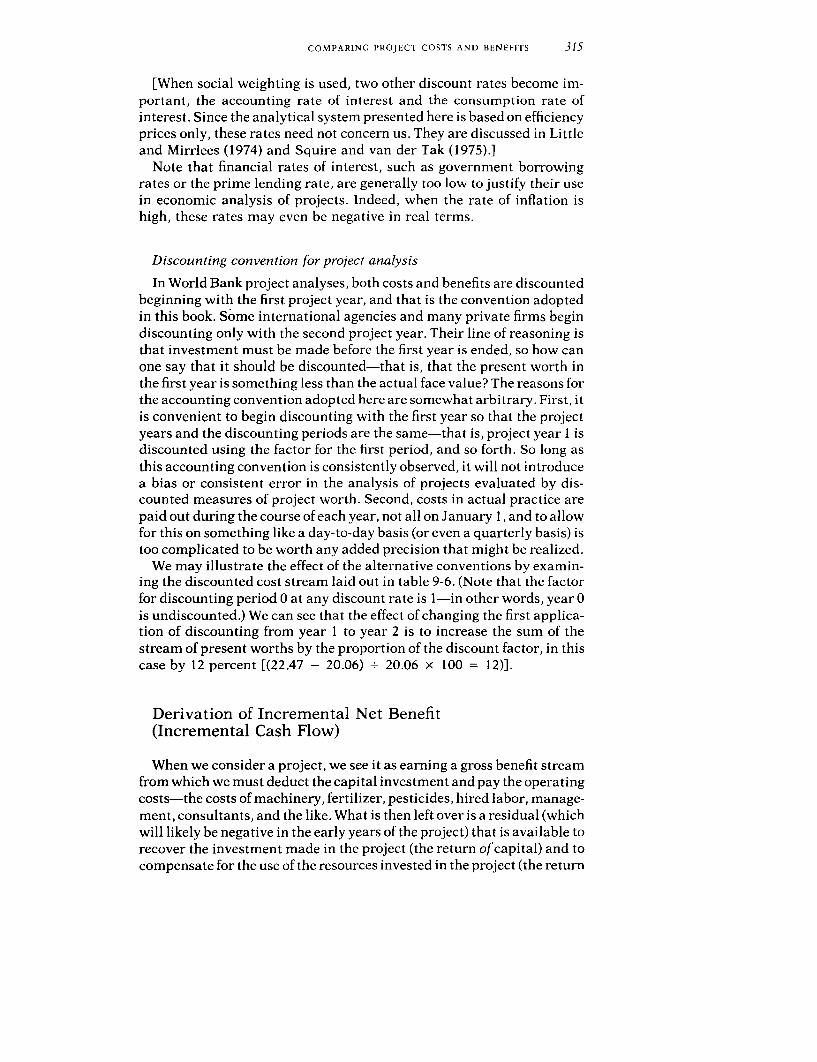
COMPARING PROJECT COSTS AND BENEFITS 315
[When social weighting is used, two other discount rates become im-portant, the accounting rate of interest and the consumption rate ofinterest. Since the analytical system presented here is based on efficiencyprices only, these rates need not concern us. They are discussed in Littleand Mirrlees (1974) and Squire and van der Tak (1975).]
Note that financial rates of interest, such as government borrowingrates or the prime lending rate, are generally too low to justify their usein economic analysis of projects. Indeed, when the rate of inflation ishigh, these rates may even be negative in real terms.
Discounting convention for project analysis
In World Bank project analyses, both costs and benefits are discountedbeginning with the first project year, and that is the convention adoptedin this book. Some international agencies and many private firms begindiscounting only with the second project year. Their line of reasoning isthat investment must be made before the first year is ended, so how canone say that it should be discounted-that is, that the present worth inthe first year is something less than the actual face value? The reasons forthe accounting convention adopted here are somewhat arbitrary. First, itis convenient to begin discounting with the first year so that the projectyears and the discounting periods are the same-that is, project year I isdiscounted using the factor for the first period, and so forth. So long asthis accounting convention is consistently observed, it will not introducea bias or consistent error in the analysis of projects evaluated by dis-counted measures of project worth. Second, costs in actual practice arepaid out during the course of each year, not all on January 1, and to allowfor this on something like a day-to-day basis (or even a quarterly basis) istoo complicated to be worth any added precision that might be realized.
We may illustrate the effect of the alternative conventions by examin-ing the discounted cost stream laid out in table 9-6. (Note that the factorfor discounting period 0 at any discount rate is 1-in other words, year 0is undiscounted.) We can see that the effect of changing the first applica-tion of discounting from year I to year 2 is to increase the sum of thestream of present worths by the proportion of the discount factor, in thiscase by 12 percent [(22.47 - 20.06) . 20.06 x 100 = 12)].
Derivation of Incremental Net Benefit(Incremental Cash Flow)
When we consider a project, we see it as earning a gross benefit streamfrom which we must deduct the capital investment and pay the operatingcosts-the costs of machinery, fertilizer, pesticides, hired labor, manage-ment, consultants, and the like. What is then left over is a residual (whichwill likely be negative in the early years of the project) that is available torecover the investment made in the project (the return of capital) and tocompensate for the use of the resources invested in the project (the return

316 MEASURES OF PROJECT WORTH
Table 9-6. Discounting from Project Year Iand from Project Year 2 Compared(currency units)
Discounting fromn year I Discounting from year 2
Discount- Discount Present Discount- Discournt PresentProject ing factor *vorth ing factor wvortlyear Amount period 12% 12% period 12% 12%
1 1.09 1 0 893 0.97 0 1.000 1.092 4.83 2 0.797 3 85 1 0.893 4.313 5.68 3 0.712 4.04 2 0.797 4.534 4.50 4 0.636 2.86 3 0.712 3.205 1.99 5 0.567 1.13 4 0.636 1.276 0.67 6 0.507 0.34 5 0.567 0.387 0.97 7 0.452 0.44 6 0.507 0.498 1 30 8 0.404 0.53 7 0.452 0.599 1.62 9 0.361 0.58 8 0.404 0.6510-30 1 95, 10-30 2 .7 2 7 b 5.32 9-29 3 054' 5.96Total 63 60 8.056 20.06 9.022 22.47
a Annual amount for years 10 through 30 inclusive To reach column total, this amountmust be included 21 times.
b. Present worth of an annuity factor for years 10 through 30 inclusive See the subsec-tion on "Present worth of a stream of future income" for method of computation.
c. Present worth of an annuity factor for years 9 through 29 inclusive. See the subsectionon "Present worth of a stream of future income" for method of computation.
to or on capital). This residual is the net benefit stream. Deducting thewithout-project net benefit gives the incremental net benefit stream.These streams are commonly called cash flows because discounted mea-sures of project worth were originally developed for use in business. Thenet benefit flow was distinguished from the profit of the business partlyby the fact that no allowance for depreciation was taken from the benefitstream, which thus included all the cash generated.
The definition of incremental net benefit or incremental cash flowapplies specifically to investment analysis. Accountants often have asomewhat different definition in mind when they use the term. Inaccounting, the cash flow is essentially the sum of the profit plus thedepreciation allowance, usually computed after payment of taxes.
The major characteristic of the incremental net benefit stream orincremental cash flow is that it includes, without differentiating, boththe return of capital and the return to capital. In other words, to computethe incremental net benefit or cash flow we do not deduct from the grossbenefit any allowance for depreciation (that is, return of capital) nor anyallowance for interest on the capital employed that has been supplied bythe entity for which we are doing the analysis.
We do not deduct depreciation because the incremental net benefitstream already allows for the return of capital over the life of the project.Depreciation is an accounting concept necessary when accounts are to beprepared for one year at a time (not prepared as a projection over the lifeof the project) and must include an allowance for the capital use during

COMPARING PROJECT COSTS AND BENEFITS 317
each year. (How the discounted cash flow methodology automaticallyallows for the return of capital in determining the worth of a project andthus eliminates the need for year-to-year depreciation is illustrated inmore detail in the section "What Happened to Depreciation?," below.)
We do not deduct interest on the capital supplied by the entity forwhich we are doing the analysis because in effect the result of a dis-counted cash flow analysis is the allowance for the return to the entity'scapital. If we compute net present worth, we are determining whatwould be left over after allowing for some specified rate of return to theentity's own capital-the interest, if you like. When we compute aninternal rate of return, this is the return to the entity's own capital and, ina sense, is the interest which that capital earns. (More precisely, it is theweighted average return to the entity's own capital engaged over the lifeof the project.) When we calculate the net benefit-investment ratio, weare comparing the present worth of the benefit we expect to gain with thepresent worth of the investment. Thus, interest is not a cost in derivingthe cash flow. Rather, it is the return we assume when we discount toobtain the net present worth or the net benefit-investment ratio and, inthe case of internal rate of return, it is the answer we obtain from ourcalculations.
There are two important differences in the manner in which we derivethe incremental net benefit when we are carrying out an economic, asopposed to a financial, analysis. The first is that in economic analysistaxes are transfer payments within the society, not payments for re-sources used in production (see chapter 7). Hence, taxes are not deductedas a cost when deriving the incremental net benefit stream as the basis onwhich to. compute the productivity of capital. To the whole economy,taxes are a part of the "benefit" available to the society as a result of thecapital invested in the project, and they may be channeled by the societytoward whatever purpose the society decides is best.
In contrast, in financial analysis duties and other indirect taxes are acost that the individual entity must pay before arriving at the amountavailable to recover its capital and to compensate it for the use of itscapital (that is, its incremental net benefit or incremental cash flow).Hence, duties and other indirect taxes are a cost like any other expendi-ture, and they are deducted to arrive at the net benefit before financing.This stream then becomes the remuneration for all resources engaged inthe project at market prices, without regard to financing or income taxes.
The second important difference in deriving the incremental net bene-fit in economic as opposed to financial analysis is that in financial analy-sis we generally must account for outside capital borrowed by the entitythat is undertaking the project-whether the entity is a farmer, an indi-vidual business, or the shareholders of a corporation taken as a group. Infinancial analysis, when borrowed capital is received it is usually enteredin the account as a kind of "benefit" received or "negative cost." Then,when a repayment of principal or a payment of interest is made to theoutside supplier of capital, it is deducted from the gross return as a costin deriving the incremental net benefit or incremental cash flow after

318 MEASURES OF PROJECT WORTli
financing. This stream thus becomes the remuneration available for theentity's own capital (its equity) aftcr financing. (Examples may be seen intables 4-19 and 5-6.) The question of financing does not arise in economicanalysis because we assume that all resources employed in the projectbelong to someone within the society-hence, there are no "outside"suppliers of capital.
Also note that, if the entity pays income taxes, these must then bededucted to arrive at the incremental net benefit after financing andtaxes, which is the remuneration for the entity's own capital (equity)after financing and taxes.
There may be occasions when the analyst would like to look at thereturn to the society from a project funded by borrowed foreign capital.The kind of economic analysis outlined here is a valid indicator of projectworth and will give the correct ranking of projects if the money borrowedfrom abroad may be used for any of a wide range of projects (or at least ifthe lender agreed to supply a stipulated amount of money contingent onthe borrower's spending the money on a particular project selected byjoint agreement from a wide range of alternatives). But if a foreigncreditor is only prepared to lend for one particular project that it hasstipulated in advance, then the project analyst may want to determinethe return to the society's own capital from participation in the project.He can do this by treating the society as a kind of corporate entity inwhich the citizens are the shareholders and by determining the netbenefit after financing, from which he can calculate the return to thesociety's own capital.
Although the incremental net benefit stream as it is derived for projectanalysis has by convention been called the cash flow, it may includenoncash elements. In economic analysis of agricultural projects, themost important of these noncash items are the values of home-consumedproduction and of wages in kind. These might appear in a settlementproject, for example, in which unemployed agricultural laborers areestablished on small holdings. One cost they might incur would be wagespaid in kind. Furthermore, because the settlers could now earn a goodliving, their income would be considerably above the opportunity cost oftheir labor. If this is so, the excess value of the home-consumed produc-tion over and above the opportunity cost of their labor would representnot a cost of production but an incremental benefit available to remuner-ate capital and would be included in the cash flow. This would be trueeven if a settler's family were to eat its entire production (we say nothingin economic analysis based on efficiency prices about who actually re-ceives the incremental net benefit; this point was taken up in more detailin chapters 1 and 7).
It is worth repeating a point made earlier. If cost, including investmentcost, is subtracted from benefit during the early years of a project, theresult will likely be a negative figure-that is, investment cost and initialoperating cost will be larger than the benefit. The project will then have anegative incremental net benefit stream or incremental cash flow. Thetechnical term "negative benefit" may take a bit of getting used to, but itreally causes no trouble.

COMPARING PROJECT COS1S AND BENEFITS 319
Perhaps the tabulation in figure 9-1 and the examples in tables 9-7 and9-8 (table 9-8 shows the separate income statements for the income taxesreported in table 9-7) can make the derivation of the incremental netbenefit or cash flow clearer. The reader may also wish to review thediscussions about how to derive the incremental net benefit from farmbudgets (chapter 4) and from processing industry accounts (chapter 5).
Net Present Worth
The most straightforward discounted cash flow measure of projectworth is the net present worth (often abbreviated as NPW). This is simplythe present worth of the incremental net benefit or incremental cash flowstream. (For a more formal mathematical statement, see the appendix tothis chapter.) The net present worth may also be computed by finding thedifference between the present worth of the benefit stream less the pres-ent worth of the cost stream, with both cost and benefit defined as in theprevious section on deriving the incremental net benefit. This, however,requires somewhat more calculation.
Net present worth may be interpreted as the present worth of theincome stream generated by an investment. In financial analysis, it is thepresent worth of the income stream accruing to the individual or entityfrom whose point of view the analysis is being undertaken-say, the farmfamily or the processing firm. In economic analysis, it is the presentworth of the incremental national income generated by the investment.
Economists are somewhat inconsistent in their terminology for thismeasure. It is often referred to as the net present value (or NPV). In thisbook we will refer to it as the net present worth to emphasize the parallelwith the discounting technique.
To calculate the net present worth requires determination of theappropriate discount rate along the lines discussed in the previous sec-tion (the subsection "Choosing the discount rate").
We may illustrate computation of the net present worth by referring tothe costs and benefits of the Philippine Ilocos Irrigation Systems Im-provement Project summarized in tables 9-9 and 9-10. (I have slightlymodified the figures to make the computations come out even.)
A group of improvements is to be made in several irrigation systems inthe Ilocos region of northern Luzon. An investment totaling the equiva-lent of US$18.09 million is to be made over a period of five years. Afterthat, there is an annual operation and maintenance cost equivalent toUS$0.34 million. The benefit arises from increased crop production. Wewill carry out the analysis assuming a project life of 30 years. (There islittle reason to carry it out any further; we will return to this point in thesection on "Length of the Project Period," below.)
In table 9-9, the present worth of the gross cost stream discounted at 12percent is found to be US$20.06 million. Similarly, the present worth ofthe incremental production stream at 12 percent is found to be US$29.64million. Subtracting the present worth of the cost stream from the pres-ent worth of the benefit stream gives a difference of US$9.58 million,

Figure 9-1. Elements of Net Benefit
From the standpoint of financtal analysis (all prices are market prices including taxes and subsidies)
Capital equipmentand buildings
Cash operating expensesfor goods sold
Cash sales (net of or consumed Net benefit beforesales taxes) Fertilizer financing
Credit sales (net of Electricity (remuneration forsales taxes) _ Maintenance supplies , all resources
Price of home-consumed Wages engaged, includingproduction Social security return of capital and
Subsidies Wages in kind return to capital)Selling, general, and
administrativeexpenses
SalariesBonuses Net benefit afterConsulting fees financingInsurance Net financing [remuneration for
Change in inventories Loans received (+) entity's own capitalRaw materials Debt service (equity) before incomeFinished goods + Repayment of - taxes, including
Duties and other principal ( ) _ return of entity's ownindirect taxes Interest I-) capital (equity) and
Accounts receivable (-) return to entity's ownAccounts pavable (+) capital (equity)
before taxes]
Net benefit afterfinancing and taxes[remuneration for
- Income taxes - entity's own capital(equity) after financingand taxes, includingreturn of entity's owncapital (equity) andreturn to entity's owncapital (equity)after taxes]

From the standpoint of economic analysis (some values may be shadow prices):
Capital equipment andbuildings
Operating expenses forValue of output I goods sold or Net benefit
sold consumed, including , (remunerationValue of home-consumed wages in kind for all society'sproduction Selling, general, and resources engaged,administrative including returnexpenses of capital and
Change in inventories return to capital)

Table 9-7. Derivation of Incremiiential Net Benefit(currencv units)
Fitancial accotunt Economic accounzta
Usitng shadowv exchange rate Using stantdard conversionl factor
With project With project With projectWithout Withouit Without
Itemn project Year 1 Year x Year z project Year ] Year x Year z project Year 1 Year x Year z
Value of outputb Inflow7v (gross benefit)
Revenue'Cash sales 1,000 1,000 3,000 3,000 1,200 1,200 3,600 3,600 1,000 1,000 3,000 3,000Credit sales 100 100 300 300 120 120 360 360 100 100 300 300Home-consumed production 200 200 300 300 240 240 360 360 200 200 300 300
Off-farm income' 200 0 0 0 100 0 0 0 83 0 0 0Subsidies' 50 50 125 125 Omit' Omit Omit Omit Omit Omit Omit OmitTotal inflow 1,550 1,350 3,725 3,725 1,660 1,560 4,320 4,320 1,383 1,300 3,600 3,600Cash operating expenses Ouitfluo (gross cost)
Goods and services other than laborFertilizerF 50 100 300 300 60 120 360 360 50 100 300 300Electricity"' 50 50 100 100 56 56 112 112 47 47 93 93Maintenance supplies' 200 300 550 550 220 330 605 605 183 275 504 504Remuneration for labor (except that
belonging to owners of the entitv)Wages' 100 150 200 200 50 75 100 100 42 62 83 83Social securityk 15 22 30 30 Omit Omit Omit Omit Omit Omit Omit OmitPayment in kind' 25 40 60 60 12 20 30 30 10 17 25 25
Selling, general, and administrative expensesSalaries 10 20 20 20 10 20 20 20 8 17 17 17Bonuses 0 0 0 0 0 0 0 0 0 0 0 0Consulting and management fees 0 0 0 0 0 0 0 0 0 0 0 0Insurance 10 15 15 15 10 15 15 15 8 12 12 12Training and research 0 0 0 0 0 0 0 0 0 0 0 0

Duties and indirect taxesm0 100 0 0 Omit Omit Omit Omit Omit Omit Omit Omit
Increase (decrease) in gross fixed assetsCapital equipmentn 0 2,000 0 ( 180) 0 2,400 0 ( 216) 0 2,000 0 ( 180)Site improvement' 0 100 0 0 0 100 0 0 0 83 0 0
Increase (decrease) in inventoriesRaw materialsP 0 100 100 ( 200) 0 120 120 ( 240) 0 100 100 ( 200)Finished goodsP 0 250 300 ( 550) 0 300 360 ( 660) 0 250 300 ( 550)
Total outflow 460 3,247 1,675 345 418 3,556 1,722 126 348 2,963 1,434 104
Net benefit before financingTotal 1,090 (1,897) 2,050 3,380 1,242 (1,996) 2,598 4,194 1,035 (1,663) 2,166 3,496Incremental - (2,987) 960 2,290 - (3,238) 1,356 2,952 - (2,698) 1,131 2,461
FinancingLong-term loans received 0 1,000 0 0 Omit Omit Omit Omit Omit Omit Omit OmitIncrease (decrease) in short-term loans 0 0 0 0 Omit Omit Omit Omit Omit Omit Omit OmitInterest received 0 0 0 0 Omit Omit Omit Omit Omit Omit Omit OmitIncrease (decrease) in accounts payable
and other short-term liabilities 0 60 60 ( 120) Omit Omit Omit Omit Omit Omit Omit OmitRepayment of long-term loansq 0 0 ( 46) 0 Omit Omit Omit Omit Omit Omit Omit OmitInterest paymentsq 0 0 ( 115) 0 Omit Omit Omit Omit Omit Omit Omit OmitLoan commitment fees 0 0 0 0 Omit Omit Omit Omit Omit Omit Omit OmitDecrease (increase) in accounts receivable 0 ( 10) ( 10) 20 Omit Omit Omit Omit Omit Omit Omit OmitDecrease (increase) in other short-term assets
except cash 0 0 0 0 Omit Omit Omit Omit Omit Omit Omit OmitNet financing 0 1,050 ( 111) ( 100) Omit Omit Omit Omit Omit Omit Omit Omit
Net benefit after financingTotal 1,090 ( 847) 1,939 3,280 Omit Omit Omit Omit Omit Omit Omit OmitIncremental - (1,937) 849 2,190 Omit Omit Omit Omit Omit Omit Omit Omit
Incomne taxationIncome taxes paid' 286 77 758 804 Omit Omit Omit Omit Omit Omit Omit Omit
Net benefit after financing and taxesTotal 804 ( 924) 1,181 2,476 Omit Omit Omit Omit Omit Omit Omit OmitIncremental - (1,728) 377 1,672 Omit Omit Omit Omit Omit Omit Omit Omit
(Table notes on the following pages.)

324 MEASURES OF PROJECT WORTHI
(Notes to Table 9-7)
Note: The figures in this table are illustrative and do not represent any real entity. Theyare assumed to be denominated in local currency. Year I is the first year of the project, yearx is the first full year of operation, and year z is the terminal year of the project. The tablefollows the general format of table 5-6, which may also be consulted. Here and in table 9-8,the accounting convention of indicating negative numbers by parentheses has beenadopted.
a. For a discussion of the principles of economic valuation, see chapter 7. The foreignexchange premium is assumed to be 20 percent. Thus, when using the shadow exchangerate to obtain economic values, the financial price of all traded items is multiplied by I plusthe foreign exchange premium stated in decimal terms, or 1.2 (I + 0.2 = 1 2). When usingtheconversion factor toobtain economic values, the financial price ofall nontraded items ismultiplied by a standard conversion factor of 0.833 (I - 1.2 = 0.833).
b. All output is assumed to be of tradable items.c. Sales are shown net of sales discounts and returned goods and net of sales taxes. Credit
sales are treated as a real resource use because it is assumed that the output has beenconsumed.
d. Off-farm income is included to account correctly for the benefit forgone in giving upoff-farm income to participate in the project. Although especially applicable to farmaccounts, a comparable entry might be included for small firms, in which event salarieswould apply only to salaried employees In the economic account, the off-farm income isassumed to come from unskilled labor services provided by the family and thus to have thesame value as hired farm labor; it is shadow-priced at half the market value (see note k).
e. These are direct subsidies. When indirect subsidies operate to change the marketprices of items, the financial prices are adjusted to economic values according to theprocedures for valuing traded or nontraded items as appropriate.
f. Items marked "Omit" are included in calculating the financial incremental net benefit(incremental cash flow), but they are not included when calculating the economic in-cremental net benefit.
g. Fertilizer is assumed tobe entirely a traded item, although application costs would nodoubt require expenditure for nontraded items
h. For electricity, it is assumed that 60 percent of the v'alue arises from traded sourcessuch as oil and generating equipment and that 40 percent arises from nontraded sourcessuch as labor and local construction materials. Thus, when the shadow exchange rate isused, 60 percent of the value of electricity is treated as a traded item and is multiplied by Iplus the foreign exchange premium stated in decimal terms, and 40 percent of the value ofelectricity is treated as a nontraded item and is carried to the economic account unchangedtoobtain the economic value of electricity of56 in the without-project situation [I + 0.2 =1.2; (50 x 0.6 x 1.2) + (50 x 0.4) = 56]. Similarly, when the conversion factor is used, 60percent of the value of electricity is treated as a traded item and is carried to the economicaccount unchanged, and 40 percent of the value of electricity is treated as a nontraded itemand is multiplied by the standard conversion factor of I divided by I plus the foreignexchange premium stated in decimal terms to obtain the economic value of electricity of47in the without-project situation [I - (I + 0 2) = 0.833: (50 x 0.6) + (50 x 0.4 x 0.833) =
47].i. Maintenance supplies are assumed to be half traded and half nontraded. A valuation
method parallel to that outlined for electricity in note i is followed. Thus, when the shadowexchange rate is used, the economic value in the without-project situation is 220 [(200 x 0.5x 1.2) + (200 x 0.5) = 220]. When the conversion factor is used, the economic value in thewithout-project situation is 183 [(200 x 0.5) + (200 x 0.5 x 0.833) = 183]. For conve-nience, maintenance supplies are shown only as a cash operating expense, although inpractice some maintenance would also be included among the selling, general, and ad-ministrative expenses
j. The shadow wage rate is assumed to be half the market wage. Thus, when the shadowexchange rate is used, the market wage used in the financial analysis is multiplied by 0.5 toobtain the economic wage of50 in the without-project situation (100 x 0.5 - 50) When theconversion factor approach is used, the market wage used in the financial analysis is firstmultiplied by 0.5 and then multiplied by the standard conversion factor to obtain theeconomic wage of 42 in the without-project situation (100 x 0 5 x 0.833 = 42)
(Table niotes cozlintnze on the following page.)

COMPARING PROJECT COSTS AND BENEFITS 325
Table 9-8. Income Statementsfor Income Taxes Reported in Table 9-7(currency units)
With projectWithoutproject Year I Year x Year z
Revenue-sales 1,100 1,100 3,300 3,300Total revenue 1,100 1,100 3,300 3,300
Cash operating expenses 415 622 1,180 1,180Selling, general, and administrative
expenses 20 35 35 35Noncash operating expenses-
depreciationa - 200 200 200Total operating expenses 435 857 1,415 1,415
Nonoperating income and expensesInterest paid 0 0 115 0Duties and indirect taxes 0 100 0 0Subsidies ( 50) ( 50) ( 125) ( 125)Total nonoperating expenses ( 50) 50 ( 10) ( 125)
Income (profit) before income taxes 715 193 1,895 2,010Income taxes 286 77 758 804Net income (profit) after taxes 429 116 1,137 1,206
Note: Income taxes are assumed to be 40 percent of income (profit) before taxes. Theformat here follows that of table 5-2.
a. Depreciation is allocated on a ten-year, straight-line basis and is charged only on aninvestment of 2,000.
k. Social security is considered to be a direct transfer payment and is omitted from theeconomic account.
1. Since payment in kind is a form of labor cost, it should be shadow-priced to reflect theopportunity cost of labor. This would mean shadow-pricing the payment in kind in thesame manner as for the money wage, in this case at half the financial wage. Since it is theopportunity cost that determines the shadow xvage rate, the method of valuing the paymentin kind would remain the same even if the payment in kind were made in a tradablecommodity such as food grain.
m. Recall that sales are shown net of sales taxes. If this were not the case, there would bean entry for sales taxes received and for sales taxes remitted to the government in thefinancial account, but these entries would be a direct transfer and thus would not beincluded in the economic account. Often capital equipment is shown inclusive of duties infinancial accounts. If this is the case, duties would be deducted before calculating thceconomic value and would not appear as a separate entry in the economic accounts.
n. Capital equipment is assumed to be net of duties (which are shown separately) and toconsist entirely of traded items, although installation costs would no doubt require expen-diture for nontraded items. In year z, the negative entry for the capital equipment repre-sents the residual value.
o. Assumed to involve only nontraded items.p. Assumed to be entirely traded items.q. The debt service payments are calculated for the second year of a twelve-year loan of
1,000 at 12 percent interest assuming a constant payment of 161 a year.r. Income taxes are assumed to be 40 peicent of income (profit) before taxes. The pro
forma income statements are given in table 9-8 following the format of table 5-2. Thedepreciation is allocated on a ten-year, straight-line basis and is charged only on aninvestment of 2,000.

Table 9-9. Computation of Net Present Worth Subtracting the Present Worth of the Gross Incremzental Cost from thePresent Worth of the Value of Incremental Production, Ilocos Irrigation Systems Improvement Project, Philippines
(millions of US$)
Incremental costValue of
Operation Discount Present incremental Discount PresentCapital and Produc- factor wvorth production factor worth
Year items maintenance tiort Gross 12% 12% (gross benefit) 12% 12%
1 1.09 0 0 1.09 0.893 0.97 0 0.893 0
2 4.83 0 0 4.83 0.797 3.85 0 0.797 0
3 5.68 0 0 5.68 0.712 4.04 0 0.712 0
4 4.50 0 0 4.50 0.636 2.86 0 0.636 0
5 1.99 0 0 1 99 0.567 1.13 0 0.567 0
6 0 0.34 0.33 0.67 0.507 0.34 1.67 0 507 0.85
7 0 0.34 0.63 0.97 0.452 0.44 3.34 0.452 1.51
8 0 0.34 0 96 1.30 0.404 0.53 5.00 0.404 2.02
9 0 0 34 1.28 1.62 0.361 0.58 6.68 0.361 2.41
10-30 0 0.34' 1.61P 1.95' 2.727" 5.32 8.38" 2 .7 2 7 b 22.85
Total 18 09 8.50 37.01 63.60 8 056 20 06 192.67 8.056 29.64
Net present iworth at 12 perce1t = US$29.64 - US$20 06 = US$+ 9.58
US$ U.S dollars. a. Annual amount for years 10 through 30 inclusive. To reach column total,
Source: Adapted from World Bank, "Philippines: Appraisal of the National this amount must be included 21 times.
Irrigation Systems Improvement Project: 1," 1488a (Washington, D.C., 1977: b. Present worth of an annuity factor for years 10 through 30 inclusive. See
restricted circulation), annex 20, tables 2 and 6. the subsection on "Present worth of a stream of future income" for method of
computation.

COMPARING PROJECT COSIS ANI) BENEFITS 327
which is the net present worth at a 12 percent discount rate (29.64 -20.06 = 9.58).
Two points about the layout of tables 9-9 and 9-10 and the computationshould be noted. Opposite the entry for the tenth through the thirtiethyears, the annual amount is entered in the undiscounted cost and benefitcolumns. To reach the undiscounted total in these columns, the annualamount must be included for each year from the tenth through thethirtieth years, or 21 times. But the present worth entered in the line forthe tenth to the thirtieth years is not an annual amount; rather, it is thetotal present worth of the stream for the whole twenty-one-year period.This convention for table layout is followed throughout chapters 9 and10. Note, too, that the total of the discount factors cannot be taken andmultiplied by the total of the cost or benefit stream to obtain the presentworth. In the gross cost stream in table 9-9, for example, the presentworth of US$20.06 million cannot be reached by multiplying the undis-counted total of the gross cost, US$63.60 million, by the total of thediscount factors, 8.056 (63.60 x 8.056 4 20.06). The year-by-year proce-dure must be followed. Including the total of the present worth factors inthe tables serves only as an internal check. The analyst knows he hasdetermined the factors correctly if they add to the present worth of anannuity factor for the final year of the project.
Although the net present worth may be computed by subtracting thetotal discounted present worth of the cost stream from that of the benefitstream, it is easier and usual practice to compute it by discounting theincremental net benefit stream or incremental cash flow. Table 9-10illustrates how this works in the case of the Philippine irrigation exam-ple. The gross incremental cost in each year is subtracted from the valueof incremental production to obtain the incremental net benefit, or cashflow. Thus, in year 1 the gross incremental cost is US$1.09 million, andthere is no incremental production, so the incremental net bencfit or cashflow is US$- 1.09 million (0 - 1.09 = - 1.09). As another example, inyear 7 the gross incremental cost is US$0.97 million, and the value ofincremental production is US$3.34 million, so the incremental net bene-fit or cash flow is US$ + 2.37 million (3.34 - 0.97 = 2.37). Summing thepresent worths of the incremental net benefit stream, or cash flow, givesus a value of US$+9.58 million. This is exactly the same amount weobtained when we subtracted the present worth of the gross incrementalcost from the present worth of the value of incremental production intable 9-9. Deriving the incremental net benefit, or cash flow, first andthen discounting, however, is the simpler computational procedure.
A considerable advantage of discounted cash flow measures such as thenet present worth, the internal rate of return, or the net benefit-investment ratio is that it makes no difference at all at what point in thecomputation the netting out takes place. To obtain the incremental netbenefit, the analyst may subtract gross cost from gross benefit, the invest-ment cost from the net benefit, or follow any other computational patternthat suits the analyst's analytical needs-provided only that doublecounting is avoided. In contrast, for the benefit-cost ratio discussed later

Table 9-10. Computation of Net Present Worth Discounting the Incremental Net Benefit Stream(Cash Flow), Ilocos Project(millions of US$)
Incremental cost Value ofincremental
Operation production Incremental Discount PresentCapital and Produc- (gross net benefit factor worth
Year items maintenance tion Gross benefit) (cash flowv) 12% 12%
1 1.09 0 0 1.09 0 - 1.09 0.893 - 0.972 4.83 0 0 4.83 0 - 4.83 0.797 - 3.853 568 0 0 5.68 0 - 5.68 0.712 - 4.044 4.50 0 0 4.50 0 - 4.50 0.636 - 2.865 1.99 0 0 1.99 0 - 1.99 0.567 - 1136 0 0.34 033 067 1.67 + 1.00 0.507 + 0.517 0 0.34 0.63 0.97 3.34 + 2.37 0.452 + 1.078 0 0.34 0.96 1.30 5.00 + 3.70 0.404 + 1.499 0 0.34 1.28 1.62 6.68 + 5.06 0.361 + 1.8310-30 0 0.34' 1.61a 1.95a 8.38a + 643a 2 7 2 7 b + 17.53Total 18.09 8.50 37.01 63.60 192.67 + 129.07 8.056 + 9.58
Net present wvorth at 12 percent = US$ + 9.58
Source: Same as table 9-9. b Present worth of an annuity factor for years 10 through 30 inclusive. Seea Annual amount foryears 10 through 30inclusive. Toreach column total, the subsection on "Present worth of a stream of future income" for method of
this amount must be included 21 times. computation.

COMPARING PROJECT COSTS AND BENEFITS 329
in this chapter, the manner in which costs and benefits are netted outmakes a difference in the ratio value. (We will show a numerical illustra-tion of this in the section on the benefit-cost ratio, below.)
Suppose the net present worth had worked out to be negative? Then wewould have a case in which, at the discount rate assumed, the presentworth of the benefit stream is less than the present worth of the coststream-that is, insufficient to recover investment. It would be better toput the money in a bank at the assumed interest rate (or, more likely, toinvest it in a better project) than to invest it in the project analyzed.
The formal selection criterion for the net present worth measure ofproject worth is to accept all independent projects with a zero or greaternet present worth when discounted at the opportunity cost of capital.(Independent projects are those which are not mutually exclusive; thatis, projects of a kind that implementing one necessarily precludes im-plementing another.) An obvious problem of the net present worth mea-sure is that the selection criterion cannot be applied unless there is arelatively satisfactory estimate of the opportunity cost of capital.
No ranking of acceptable, alternative independent projects is possiblewith the net present worth criterion because it is an absolute, not rela-tive, measure. A small, highly attractive project may have a smaller netpresent worth than a large, marginally acceptable project. As long asboth have a positive net present worth and the administrative capacityand resources exist to implement both (and the projects are not mutuallyexclusive), this difference is not important. Our selection criterion tellsus to undertake both, since there will be enough money if the opportunitycost of capital has been correctly estimated. If because of lack of funds oradministrative resources we cannot undertake both, the implication isthat the opportunity cost of capital has been estimated to be too low.Then the correct response is to raise the estimate until we have only theselection of projects with net present worths that are zero or positive andfor which, in fact, there will be just sufficient investment funds.
Net present worth is also the preferred selection criterion to chooseamong mutually exclusive projects because of a possible error in ap-plying the internal rate of return measure to such projects (see chapter10, the section on "Choosing among Mutually Exclusive Alternatives").
Internal Rate of Return
Another way of using the incremental net benefit stream or in-cremental cash flow for measuring the worth of a project is to find thediscount rate that makes the net present worth of the incremental netbenefit stream or incremental cash flow equal zero. This discount rate iscalled the internal rate of return. It is the maximum interest that aproject could pay for the resources used if the project is to recover itsinvestment and operating costs and still break even. It is the "rate ofreturn on capital outstanding per period while it is invested in the

Table 9-11. Computation of Internal Rate of Return, Ilocos Project(millions of US$)
Incremental cost Value ofincremnental
Operation Discount Present production Present Incremental PresentCapital and Produc- factor wvorth (gross iworth net benefit worth
Year items maintenance tton Gross 18% 18% benefit) 18% (cash flowv) 18%(1) (2) (3) (4) (5) (6) (7) (8) (9) (10) (11)
1 1.09 0 0 1.09 0.847 0.92 0 0 - 1.09 - 0.922 4.83 0 0 4.83 0.718 3.47 0 0 - 4.83 -3.473 5.68 0 0 5.68 0.609 3.46 0 0 - 5.68 - 3.464 4.50 0 0 4.50 0.516 2.32 0 0 - 4.50 -2 325 1.99 0 0 1.99 0.437 0.87 0 0 - 1.99 - 0.876 0 0.34 0.33 0.67 0.370 0.25 1.67 0.62 + 1.00 + 0.377 0 0.34 0.63 0.97 0.314 0.30 3.34 1.05 + 2.37 +0.748 0 0.34 0.96 1.30 0.266 0 35 5.00 1.33 + 3.70 + 0.989 0 0.34 1.28 1.62 0.225 0.36 6.68 1 50 + 5.06 + 1.1410-30 0 0.34" 1.61P 1.95a 1 .2 1 4 b 2.37 8 38" 10.17 + 6.43a +7.81Total 18.09 8.50 37.01 63.60 5.516 14.67 192.67 14.67 + 129.07 0
Net present worth at 18 percent = US$14.67 - US$14.67 = US$0Internal rate of return = 18 percent
Source Same as table 9-9. b. Present worth of an annuity factor for years 10 through 30 inclusive. Seea. Annual amount for years 10 through 30 inclusiv'e. To reach column total, the subsection "Present worth of a stream of future income" for method of
this amount must be included 21 times. computation.

COMPARING PROJECI COSTS AND BENEFITS 331
project" (Merrett and Sykes 1963, p. 38). (For a more formal mathemati-cal statement, see the appendix to this chapter.)
The internal rate of return is a very useful measure of project worth. Itis the measure the World Bank uses for practically all its economic andfinancial analyses of projects and the measure used by most other inter-national financing agencies.
To avoid confusion between use of the internal rate of return in finan-cial analysis and use of the same techniques in economic analysis, we willadopt a distinguishing terminology. When the internal rate of return isused in financial analysis, we will refer to the result as the "financial rateof return"; when it is used in economic analysis, we will call the result the"economic rate of return." When the emphasis of our discussion is onmethodology, however, we will refer simply to the internal rate of return.
To see how the internal rate of return is calculated, we may takeanother look at the Philippine Ilocos Irrigation Systems Improvementexample for which we derived the incremental net benefit (or in-cremental cash flow) in table 9-10. But this time, instead of discountingat 12 percent, let us discount at 18 percent, as shown in table 9-11,column 11. By selecting the 18 percent discount rate, we have driven thenet present worth of the project down to zero. Put another way, at adiscount rate of 18 percent, this project just breaks even-that is, it couldearn back all the capital and operating costs expended on it and pay 18percent for the use of the money in the meantime.
From yet another vantage point, we could have asked ourselves whatinterest rate this project would earn. In other words, what would be theearning of the money invested in this project? This earning rate of aproject is the internal rate of return.
The formal selection criterion for the internal rate of return measure ofproject worth is to accept all independent projects having an internalrate of return equal to or greater than the opportunity cost of capital.
One word of caution, however. In the case of mutually exclusive proj-ects, direct comparison of internal rates of return can lead to anerroneous investment choice. This danger can be avoided most easily byusing the net present worth criterion, but it can also be avoided bydiscounting the differences in the cash flows of alternative projects.(See chapter 10, the section on "Choosing among Mutually ExclusiveAlternatives".)
Note that an internal rate of return of a series of values such as a cashflow can exist only when at least one value is negative. If all the values arepositive, no discount rate can make the net present worth of the streamequal zero. No matter how high the discount rate, the net present worthof a series would have to be positive if it includes no negative number.
Although the internal rates of return of different projects will vary,projects cannot with confidence be ranked on the basis of the internalrate of return. Only in a very general way will the internal rate of returntell us that one project is better than another, in the sense that it contrib-utes more to national income relative to the resources used. A projectwith a 25 percent economic rate of return is likely to be a better invest-
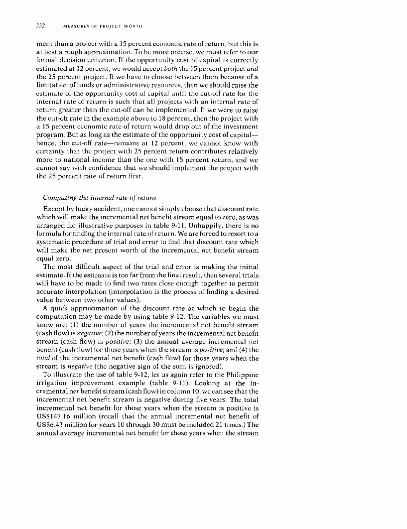
332 MEASURES OF PROJECT WORTH
ment than a project with a 15 percent economic rate of return, but this isat best a rough approximation. To be more precise, we must refer to ourformal decision criterion. If the opportunity cost of capital is correctlyestimated at 12 percent, we would accept both the 15 percent project andthe 25 percent project. If we havc to choose between them because of alimitation of funds or administrative resources, then we should raise theestimate of the opportunity cost of capital until the cut-off rate for theinternal rate of return is such that all projects with an internal rate ofreturn greater than the cut-off can be implemented. If we were to raisethe cut-off rate in the example above to 18 percent, then the project witha 15 percent economic rate of return would drop out of the investmentprogram. But as long as the estimate of the opportunity cost of capital-hence, the cut-off rate-remains at 12 percent, we cannot know withcertainty that the project with 25 percent return contributes relativelymore to national income than the one with 15 percent return, and wecannot say with confidence that we should implement the project withthe 25 percent rate of return first.
Computing the internal rate of return
Except by lucky accident, one cannot simply choose that discount ratewhich will make the incremental net benefit stream equal to zero, as wasarranged for illustrative purposes in table 9-1 1. Unhappily, there is noformula for finding the internal rate of return. We are forced to resort to asystematic procedure of trial and error to find that discount rate whichwill make the net present worth of the incremental net benefit streamequal zero.
The most difficult aspect of the trial and error is making the initialestimate. If the estimate is too far from the final result, then several trialswill have to be made to find two rates close enough together to permitaccurate interpolation (interpolation is the process of finding a desiredvalue between two other values).
A quick approximation of the discount rate at which to begin thecomputation may be made by using table 9-12. The variables we mustknow are: (1) the number of years the incremental net benefit stream(cash flow) is negative; (2) the number of years the incremental net benefitstream (cash flow) is positive; (3) the annual average incremental netbenefit (cash flow) for those years when the stream is positive; and (4) thetotal of the incremental net benefit (cash flow) for those years when thestream is negative (the negative sign of the sum is ignored).
To illustrate the use of table 9-12, let us again refer to the Philippineirrigation improvement example (table 9-1 1). Looking at the in-cremental net benefit stream (cash flow) in column 10, we can see that theincremental net benefit stream is negative during five years. The totalincremental net benefit for those years when the stream is positive isUS$147.16 million (recall that the annual incremental net benefit ofUS$6.43 million for years 10 through 30 must be included 21 times.) Theannual average incremental net benefit for those years when the stream

COMPARING PROJECT COSTS AND BENEFITS 333
Table 9-12. Method of Computing Initial Estimateof Internal Rate of Return
First, Second,determine: determine: Third, divide:
Average annual positive incremental net benefit
Total negative incremental net benefitNumber Number and use the result to select the proper column here.of years of years Then find the initial estimate opposite the appro-
incremental incremental priate number of years for the negative and thenet benefit net benefit positive incremental net benefit streams.stream is stream isnegative positive 0.1 0.2 0.3 0.4 0.5 0.6 0.8 1.0
5 - 0 12 22 30 38 >50 >501 10 0 12 21 28 34 40 50 >50
20 7 16 23 28 34 38 47 >505 - 0 10 19 25 30 40 49
2 10 0 11 18 24 29 34 42 4820 6 14 20 25 29 33 40 46
5 - 0 9 15 21 25 33 403 10 0 10 16 21 26 29 36 41
20 6 13 18 23 26 29 35 405 - 0 7 13 18 22 28 34
4 10 0 9 15 19 23 26 31 3620 6 12 17 21 24 26 31 35
5 - 0 7 12 16 19 25 295 10 0 8 13 17 21 23 28 32
20 5 12 16 19 22 24 28 31
This table assumes standardized in- + 60cremental net benefit streams with this -general time profile: +40-
z +20-
0 in * Years-20-
-40-
Source: Adapted from Schaefer-Kehnert (1979).
is positive is thus US$5.89 million (147.16 + 25 = 5.89). The total of theincremental net benefit in those years when the stream is negative isUS$ - 18.09 million. We will ignore the sign and take the sum to besimply US$18.09 million. Dividing the annual average positive in-cremental net benefit by the total negative incremental net benefit givesus 0.33 (5.89 -- 18.09 = 0.33).
In table 9-12 we can find the group of figures opposite the entry for anegative period of five years and for a positive period of twenty years, the

Table 9-13. Conmptutationi of Internial Rate of Return Illustratinig Interpolation, Ilocos Project(millions of US$)
Increniental cost Valtue ofincremental
Operation pr-oductiont lincrem2ental Discotunt Present Discount PresentCapital and Produtc- (gross net benefit factor worth factor worth
Year itemns maintenance t2on Gross benefit) (cash flow) 16% 16% 20% 20%1 1.09 0 0 1.09 0 - 1.09 0 862 - 0.94 0.833 -0 912 4.83 0 0 4.83 0 - 4 83 0.743 - 3.59 0 694 - 3.353 5 68 0 0 5.68 0 - 5.68 0.641 - 3.64 0 579 -3.294 4.50 0 0 4 50 0 - 4.50 0.552 - 2 48 0.482 - 2.175 1.99 0 0 1.99 0 1.99 0 476 -0 95 0.402 - 0 806 0 0.34 0.33 0.67 1 67 + 1.00 0.410 + 0.41 0335 +0.347 0 0.34 0.63 0.97 3.34 + 2 37 0.354 + 0 84 0.279 +0 668 0 0.34 0.96 1.30 500 + 3.70 0305 + 1 13 0233 +0.869 0 0.34 1 28 1 62 6 68 + 5.06 0.263 + 1.33 0.194 +-0.9810-30 0 0 34' 1.61 1 95n' 8.38' + 6.43' 1 570"' + 10.10 0 9 48b +6.10Total 18 09 8.50 37.01 63.60 192.67 + 129.07 6.176 + 2 21 4.979 -1.58
Internal rate of retrn" (econ0omic rate of returnr) = 16 + 4[2.21 - (2.21 + 1.58)] = 16 + 4(2.21 - 3.79) = 16 + 4(0.58) = 18.32 = 18 percent
Souirce Same as table 9-9. b. Present woirth of an annuity factor for years 10 through 30 inclusive. Scea. Annual amount for years 10 through 30 inclusive. To r each column total, subsection on "Present worth of a stream of future incomc'' for method ofthis amount must be included 21 times. computation
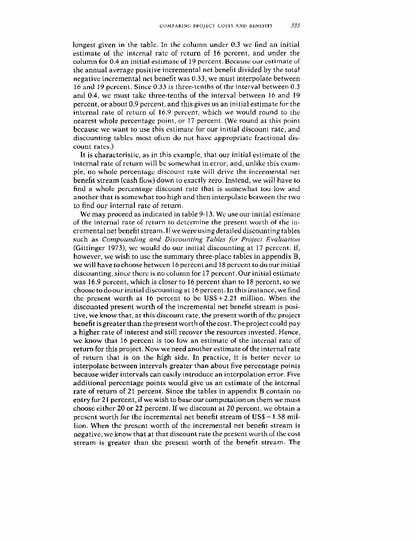
COMPARING PROJECTI COS'IS AND BENEFITS 335
longest given in the table. In the column under 0.3 we find an initialestimate of the internal rate of return of 16 percent, and under thecolumn for 0.4 an initial estimate of 19 percent. Because our estimate ofthe annual average positive incremental net benefit divided by the totalnegative incremental net benefit was 0.33, we must interpolate between16 and 19 percent. Since 0.33 is three-tenths of the interval between 0.3and 0.4, we must take three-tenths of the interval between 16 and 19percent, or about 0.9 percent, and this gives us an initial estimate for theinternal rate of return of 16.9 percent, which we would round to thenearest whole percentage point, or 17 percent. (We round at this pointbecause we want to use this estimate for our initial discount rate, anddiscounting tables most often do not have appropriate fractional dis-count rates.)
It is characteristic, as in this example, that our initial estimate of theinternal rate of return will be somewhat in error; and, unlike this exam-ple, no whole percentage discount rate will drive the incremental netbenefit stream (cash flow) down to exactly zero. Instead, we will have tofind a whole percentage discount rate that is somewhat too low andanother that is somewhat too high and then interpolate between the twoto find our internal rate of return.
We may proceed as indicated in table 9-13. We use our initial estimateof the internal rate of return to determine the present worth of the in-cremental net benefit stream. If we were using detailed discounting tablessuch as Compounding and Discounting Tables for Project Evaluation(Gittinger 1973), we would do our initial discounting at 17 percent. If,however, we wish to use the summary three-place tables in appendix B,we will have to choose between 16 percent and 18 percent to do our initialdiscounting, since there is no column for 17 percent. Our initial estimatewas 16.9 percent, which is closer to 16 percent than to 18 percent, so wechoose to do our initial discounting at 16 percent. In this instance, we findthe present worth at 16 percent to be US$+2.21 million. When thediscounted present worth of the incremental net benefit stream is posi-tive, we know that, at this discount Irate, the present worth of the projectbenefit is greater than the present worth of the cost. The project could paya higher rate of interest and still recover the resources invested. Hence,we know that 16 percent is too low an estimate of the internal rate ofreturn for this project. Now we need another estimate of the internal rateof return that is on the high side. In practice, it is better never tointerpolate between intervals greater than about five percentage pointsbecause wider intervals can easily introduce an interpolation error. Fiveadditional percentage points would give us an estimate of the internalrate of return of 21 percent. Since the tables in appendix B contain noentry for 21 percent, if we wish to base our computation on them we mustchoose either 20 or 22 percent. If we discount at 20 percent, we obtain apresent worth for the incremental net benefit stream of US$ - 1.58 mil-lion. When the present worth of the incremental net benefit stream isnegative, we know that at that discount rate the present worth of the coststream is greater than the present worth of the benefit stream. The

336 MEASURES OF PROJECT WORTH
project cannot pay such a high rate of interest and still recover theresources invested.
Just where does the real internal rate of return lie? We could find out bysuccessively narrowing down our limits until finally we find the discountrate that will make the sum exactly zero, but this would require muchrepetitive computation and the use of fractional discount factors forwhich no tables exist. Instead, we use interpolation to estimate the truevalue. (Again, interpolation is simply finding the intermediate valuebetween two discount rates we have chosen. Many readers may havelearned how to interpolate when they studied trigonometry in secondaryschool; the procedure outlined here is exactly the same.)
The rule for interpolating the value of the internal rate of return lyingbetween discount rates too high on the one side and too low on the otheris:
Present worth of incre-mental net benefit
Internal Lower Difference stream (cash flow) atrate of = discount + between the the lower discount ratereturn rate discount rates Sum of the present worths
of the incremental net bene-fit streams (cash flows)at the two discount rates,signs ignored
This procedure has been applied at the bottom of table 9-13. The lowerdiscount rate is 16 percent. The difference between the two discount ratesis the difference between 16 percent and 20 percent, or 4 percent. Thepresent worth of the incremental net benefit stream at the lower discountrate of 16 percent is US$2.21 million. The present worth at the higherdiscount rate of 20 percent is US$ - 1.58 million. The sum of the presentworths of the streams at the two discount rates, ignoring the signs, isUS$3.79 million (2.21 + 1.58 = 3.79). Hence:
Internal rate of return = 16 + 4 (2.21 . 3.79) = 16 + 4(0.58) = 18.32 =
18 percent.
As noted earlier, it is better not to try interpolation between a spreadwider than about five percentage points. The economic or financial ratesof return should always be rounded to the nearest whole percentagepoint, since the underlying projections never can justify the implicationof greater precision.
Interpolation between discount rates that bracket the true internalrate of return always somewhat overstates the true return. This is sobecause our linear interpolation technique makes the implicit assump-tion that, as we move from one discount rate to another, the internal rateof return will change following a straight line; actually, the true value ofthe internal rate of return follows a concave curvilinear function, asindicated in figure 9-2. The error introduced by interpolation is usually

COMPARING PROJECT COSTS AND BENEFITS 337
Figure 9-2. Interpolation Error, Jatiluhur Irrigation Project, Indonesia
+ 1 50+ 1.45
D 1.0
E_ +1.00S 3> n Interpolated
Cu
00
+0.12-
-0.21
-0.5015 16 17 18 19 20
Discount rate (percent)
Rp Indonesian rupiahs.Source: Adapted from World Bank, "Djatiluhur Irrigation Project," PA-37 (Washington,D.C ,1970, restricted circulation), p.26 and annex lO, p I Since this report was submitted,a spelling reform has changed the spelling of the project area to Jatiluhur.
slight and disappears when the result is rounded to the nearest wholepercentage point. Nevertheless, a final figure for the rate of return shouldalways be verified. This can be done most easily by taking advantage ofthe fact that the interpolation error becomes less and less as we approachone of the discount rates between which we are interpolating. Thus, averification procedure that reduces the computational burden is to usethe internal rate of return estimated by interpolation to discount theincremental net benefit stream once again. We can then interpolatebetween our estimated internal rate of return and the lower of thediscount rates we previously used. This procedure is illustrated in table9-14 with reference to the Jatiluhur Irrigation Project in Indonesia.Interpolating between 15 percent and 20 percent gives us an estimatedinternal rate of return of 19 percent. Discounting the incremental netbenefit stream at 19 percent shows the present worth to have a negativevalue of Rp - 0.21 thousand million. (The symbol for Indonesian rupiahsis Rp.) Interpolating again, this time between 15 percent and 19 percent,we find the estimate to be 18.48 percent, which would be rounded to thenearest whole percentage point of 18 percent. Because we know that theinterpolation process introduces very little error at this point butnonetheless does slightly overestimate the true rate of return and be-

Table 9-14. Computation of Internal Rate of Return Illustrating Interpolation, Jatiluhur Project, Indonesia(thousand millions of Rp)
Incremental Discount Present Discount Present Discount Present Discount PresentIncremental Incremental net benefit factor worth factor worth factor worth factor worth
Year cost benefita (cash flowV) 15% 15% 18% 18% 19% 19% 20% 20%
1 0.5 - - 0 5 0 870 - 0 44 0.847 - 0 42 0.840 - 042 0 833 - 0.422 2.1 04 - 17 0756 -129 0718 -122 0706 -120 0694 -1 183 3.7 0 7 - 3 0 0 658 - 1 97 0 609 - 1.83 0.593 - 1 78 0 579 - 1 744 3.7 1 3 - 2 4 0 572 - 1 37 0 516 - 1 24 0 499 - 1.20 0.482 - 1.165 2.0 1 9 - 0 1 0497 -0.05 0437 -004 0.419 -004 0.402 -0046 0.5 22 + 1 7 0432 +073 0370 +063 0352 +0.60 0335 +0.577-30 0.5b 2.6b + 2 lb 2 782' +5 84 2 019, + 4.24 1.825' +3 83 1 653' + 3.47Total 24 5 68 9 +44 4 6 567 + 1 45 5.516 +0 12 5 234 -0 21 4.978 -0 50
Internal rate of return interpolating between 15 percent and 20 percent: 15 + 5(1.45 - 1 95) = 15 + 5(0 74) = 15 + 3.70 = 18 70 = 19 percentInternal rate of return interpolating between 15 percent and 19 percent 15 + 4(1 45 - 1 66) = 15 + 4(0 87) = 15 + 3.48 = 18 48 = 18 percent
Internal rate of return interpolating between 18 percent and 19 percent 18 + (0 12 - 0 33) = 18 + 0 36 = 18.36 = 18 percent
Rp Indonesian rupiahs. b Annual amount for years 7 through 30 inclusive To reach column total,Source Same as figure 9-2 this amount must be included 24 times.a Assumes only an improvement in water control, that is, no accompany- c Present worth of an annuity factor for years 7 through 30 inclusive See
ing increase in the use of modern inputs. the subsection on "Present worth of a stream of future income" for method ofcomputation

COMPARING PROJECT COSTS AND BENEFITS 339
cause we have rounded to the lower whole percentage value, we couldconfidently stop at this point. For purposes of illustration, however, onefurther verification is made in table 9-14, by interpolating between 18and 19 percent. At 18 percent we have a positive present worth, and at 19percent a negative present worth, so we know that the internal rate ofreturn rounded to the nearest whole percentage point must be either oneor the other value. Since the interpolated value between 18 and 19percent is 18.36 percent, and we know that to be above the true rate bysome small amount, we can say with certainty that the internal rate ofreturn rounded to the nearest whole percentage point must be 18percent.
Reinvestment of returns
A frequent criticism of the internal rate of return is that there is animplicit assumption that all returns from the project will be reinvestedat the internal rate of return. This is not, in fact, the case. Instead, as wehave noted, the internal rate of return is correctly interpreted as being"the rate of return on capital outstanding per period while it is investedin the project" (Merrett and Sykes 1963, p. 38). Returns withdrawn froma project may be reinvested at any other rate or consumed withoutaffecting the internal rate of return of the project.
In some instances, the reinvestment criticism relates to projects ofdifferent duration. If there are two projects, one of ten years' durationthat yields 40 percent and another of twenty years' that yields 20 percent,which is preferable? Straight comparison would indicate the higher-yielding alternative for the shorter period. But if it were assumed thatthere would be no high-yielding project in which to reinvest the fundsgenerated by the project of shorter duration, then it is possible for returnsover the whole twenty years to be maximized by investing in the projectwith lower yield but longer duration. The investment decision in thisinstance will rest on the analyst's assumption about possible projectopportunities ten years hence. The investment decision could be guidedby determining the net present worth or internal rate of return of ex-pected costs and returns over the full twenty years, say one twenty-yearproject versus two ten-year projects.
More than one possible internal rate of return
Under certain circumstances-exceedingly rare in agricultural proj-ects-it is possible that more than one discount rate will make thepresent worth of the incremental net benefit stream equal zero. Thispossibility has been the source of considerable (and generally exagger-ated) criticism of the internal rate of return as a discounted measure ofproject worth. (No similar problem exists with the other measures ofproject worth discussed in this chapter.)
More than one solution in determining the internal rate of return canexist only when, following a period of positive cash flows sizable enough

Table 9-15. Internal Rate of Return Calculation2 Illustrating Multiple Solutions, Oil Well Project
(thousands of US$)
Increnmenital Discount Present Discount Present Discount Present Discount Present
niet benefit factor worth factor iworth factor worth factor iworth
Year (cash flow) 20% 20% 25% 25% 40% 40% 45% 45%
1-4 + 50 2.589 + 129 2.362 + 118 1.849 + 92 1.720 + 86
5 - 750 0.402 - 302 0 328 - 246 0.186 - 140 0 156 - 117
6-20 +100 1.879 + 188 1.265 + 126 0.462 + 46 0345 + 34
Total + 950 4.870 + 15 3.955 - 2 2.497 - 2 2.221 + 3
Souirce: Grant and Ireson (1964, p. 509).

COMPARING PROJECT COSTS AND BENEFITS 341
that the cumulative present worth up to that point is positive, there thenoccur negative cash flows such that the present worth at to of the cashflow from a given year onward (discounted in the normal way) is nega-tive. Under such circumstances there may be more than one discount ratethat will bring the present worth of the cash flow down to zero, althoughthis will not necessarily be the case.
Negative incremental net benefits for particular years are sometimesfound in agricultural projects. They can arise, for instance, when pumpsmust be replaced in an irrigation system or at the beginning of a replant-ing cycle in a crops project. Usually, however, the negative incrementalnet benefit flows late in the project will have to be quite large for there tobe multiple solutions. An occasional negative year, or a final year or twoof negative incremental net benefits, will almost never give rise to multi-ple solutions.
The kind of situation in which there are large negative cash flows afterthe initial investment phase of the project, although it is rare in agricul-ture, can be found in natural resources projects. To illustrate a multiplesolution, we may consider an example of such a natural resources projectgiven by Grant and Ireson (1964, pp. 509-10). Take the case of an oilcompany that is offered a lease on a group of wells for which the primaryoil reserves are close to exhaustion. The major condition of the purchaseis that the oil company must agree to undertake the injection of waterinto the underground reservoir to make possible a secondary recovery atthe time the primary reserves are exhausted. The lessor will receive astandard royalty from all oil produced from the property whether fromthe primary or secondary reserves. No immediate payment from the oilcompany is required. The company estimates it will realize US$50thousand a year for five years before exhausting the primary reserves.Then it must expend US$800 thousand for the water-injection project-the large negative cash flow-after which it will realize US$ 100 thousanda year for the following fifteen years. The internal rate of return calcula-tion for this example is shown in table 9-15.
From the standpoint of agricultural project analysis, this is a curiosityof internal rate of return theory that has virtually no practical impor-tance. In fact, I have been unable to find an agricultural example from areal project that illustrates the point, and I would appreciate learning ofsuch an example should the reader find one. If such a case exists in anagricultural project, the analytical problem can be resolved by usingeither the "extended yield" method or the "auxiliary interest rate"method. A discussion of these methods can be found in Merrett and Sykes(1963, pp. 158-65) and Grant and Ireson (1970, pp. 546-65).
Point in time for internal rate of return calculations
Internal rate of return calculations can be done from any point in time,and all points will give the same return. In our illustrations we alwayscalculate from to into the future because this simplifies the calculation.But if we chose the end of the project, for example, we could increase by
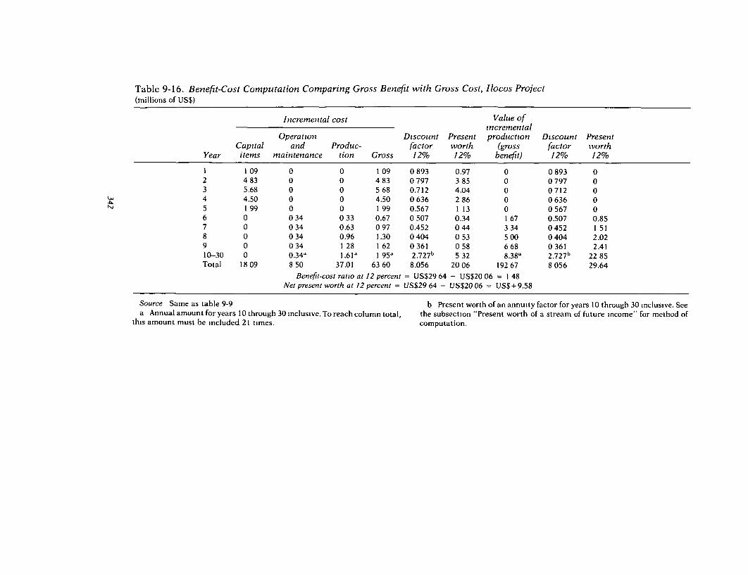
Table 9-16. Benefit-Cost Computation Comparing Gross Benefit with Gross Cost, Ilocos Project(millions of US$)
Incremental cost Value ofincremental
Operation Discount Present production Discount PresentCapital and Produc- factor wvorth (gross factor wvorth
Year items maintenance tion Gross 12% 12% benefit) 12% 12%
1 1 09 0 0 1 09 0893 0.97 0 0893 02 4 83 0 0 4 83 0 797 3 85 0 0 797 03 5.68 0 0 5 68 0.712 4.04 0 0 712 04 4.50 0 0 4.50 0636 2 86 0 0636 05 199 0 0 199 0.567 1 13 0 0567 06 0 034 033 0.67 0 507 0.34 1 67 0.507 0.857 0 034 0.63 097 0.452 044 3 34 0452 1 518 0 0 34 0.96 1.30 0 404 0 53 5 00 0 404 2.029 0 034 1 28 1 62 0361 058 668 0361 2.4110-30 0 0.34" 1.61" 1 95, 2 .7 2 7 b 5 32 8.38' 2 .7 2 7 b 22 85Total 18 09 8 50 37.01 63 60 8.056 20 06 192 67 8 056 29.64
Benefit-cost ratio at 12 percent = US$29 64 - US$20 06 = 1 48Net present worth at 12 percent = US$29 64 - US$20 06 = US$ + 9.58
Source Same as table 9-9 b Present worth of an annuity factor for years 10 through 30 inclusive. Seea Annual amount for years 1O through 30 inclusive. To reach column total, the subsection "Present worth of a stream of future income" for method of
this amount must be included 21 times. computation.

COMPARING PROJECT COSTS AND llENEFITS 343
compound interest factors all values in the incremental net benefitstream and find the interest rate that just makes the stream equal zero. Ifwe were to designate a point midway through the project period as to, wecould increase all values before the time from which we choose to work(say from t- 5 to t_,) by compound interest factors and draw down allfuture values (say from t+ I to t+ 14) by using discount factors. Again, wewould be looking for that interest rate which makes the value of theincremental net benefit stream at to equal zero.
Benefit-Cost Ratio
A third discounted measure of project worth is the benefit-cost ratio.This is the ratio obtained when the present worth of the benefit stream isdivided by the present worth of the cost stream. (For a more formalmathematical statement, see the appendix to this chapter.)
Incidentally, economists are quite inconsistent in their use of benefit-cost ratio. About half the time they say "cost-benefit" ratio. Here, how-ever, I will stick to benefit-cost ratio to emphasize the computation bywhich the measure is worked out.
The benefit-cost ratio is not commonly used in developing countries.This is because the value of the ratio will change depending on where thenetting out in the cost and benefit streams occurs. (Further on in thissection we will illustrate how this works.) The benefit-cost ratio was thefirst of the discounted measures of project worth to become well known.It is extensively employed in the United States for water resource proj-ects, although it is now increasingly being replaced by a variation of thenet present worth criterion. Many economists in developing countrieswho have studied in the United States or who are familiar with U.S.practice will know of the benefit-cost measure. By the time discountedmeasures of project worth began to be applied in developing countries,the discounted cash flow measures of net present worth and internal rateof return had become well known and were being widely used for privateinvestment. Since discounted cash flow measures do not change whendifferent conventions for netting out are used, they are easier to applyand were thus adopted by development economists.
We return to the Philippine Ilocos Irrigation Systems ImprovementProject analyzed in tables 9-9 through 9-11 to show how the benefit-costratio is calculated. In table 9-16, the gross benefit is compared with thegross cost. The present worth of the gross incremental cost stream at 12percent is found to be US$20.06 million, whereas the present worth of thevalue of incremental production or gross benefit stream is found to beUS$29.64 million. Dividing the present worth of the gross benefit streamby the present worth of the gross cost stream, we find the benefit-costratio to be 1.48 (29.64 20.06 = 1.48).
Had the benefit-cost ratio worked out to be less than I, then the presentworth of the costs at this discount rate would have exceeded the present

Table 9-17. Benefit-Cost Computation Comparing Net Benefit with Investmentplus Operation and Maintenance Cost, Ilocos Project(millions of US$)
Incremental cost Value ofincremental Net value
Operation Discount Present production Incremental of Discount PresentCapital and factor worth (gross production incremental factor worth
Year items maintenance Total 12% 12% benefit) cost production 12% 12%
1 1.09 0 1.09 0.893 0.97 0 0 0 0.893 02 4.83 0 4.83 0.797 3.85 0 0 0 0.797 03 5.68 0 5.68 0.712 4 04 0 0 0 0.712 04 4.50 0 4.50 0.636 2.86 0 0 0 0.636 05 1.99 0 1.99 0.567 1.13 0 0 0 0.567 06 0 0.34 0.34 0.507 0.17 1.67 0.33 1.34 0.507 0.687 0 0.34 0.34 0.452 0.15 3.34 0.63 2.71 0.452 1.228 0 0.34 0.34 0 404 014 5.00 0.96 4.04 0.404 1.639 0 0.34 0.34 0.361 0.12 6.68 1.28 5.40 0.361 1.9510 -30 0 0.34' 0.34' 2 .7 2 7b 0.93' 8.38a 1.6I' 6.77a 2 .7 2 7 b 1846Total 18.09 8 50 26.59 8.056 14.36 192.67 37.01 155.66 8.056 23.94
Benefit-co.st ratio at 12 percent = US$23.94 - US$14.36 = 1.67Net present worth at 12 percent = US$23.94 - US$14.36 = US$+9.58
Source: Same as table 9-9. b. Present worth of an annuity factor for years 10 through 30 inclusive. Seea. Annual amount for years 10 through 30 inclusive. To reach column total, the subsection "Present worth of a future stream of income" for method of
this amount must be included 21 times. computation.

COMPARING PROJECTI COSTS AND BENEFITS 345
worth of the benefits, and we would not have recovered our initialexpenditure plus the return on our investment from the project.
Note that the absolute value of the benefit-cost ratio will vary depend-ing on the interest rate chosen. The higher the interest rate, the smallerthe resultant benefit-cost ratio, and, if a high enough rate is chosen, thebenefit-cost ratio will be driven down to less than 1.
The formal selection criterion for the benefit-cost ratio measure ofproject worth is to accept all independent projects with a benefit-costratio of I or greater when the cost and benefit streams are discounted atthe opportunity cost of capital. In the case of mutually exclusive projects,the benefit-cost ratio can lead to an erroneous investment choice. Thedanger can be avoided most easily by using the net present worth crite-rion for mutually exclusive projects.
One convenience of the benefit-cost ratio is that it can be used directlyto note how much costs could rise without making the project economi-cally unattractive. In table 9-16, for example, we can tell by inspectionthat costs could rise by 48 percent before the benefit-cost ratio would bedriven down to 1. With a little manipulation-taking the reciprocal of thebenefit-cost ratio and subtracting it from 1-we can tell that benefitscould fall by 32 percent before the ratio would be driven down to one [ I -(1 . 1.48) = 0.32; 29.64 - (29.64 x 0.32) = 20.16; 20.16 20.06 = 1.00].In effect, this is a quick means to estimate two "switching values." (Aswitching value is the amount an element of a project can change beforethe project becomes an unacceptable investment-see the section de-voted to this topic in chapter 10.)
In practice, it is probably more common not to compute the benefit-cost ratio using gross cost and gross benefit, but rather to compare thepresent worth of the net benefit with the present worth of the investmentcost plus the operation and maintenance cost. This reflects U.S. govern-ment practice. More specifically, the ratio is computed by taking thepresent worth of the gross benefit less "associated" cost and then com-paring it with the present worth of the "project economic cost." Theassociated cost is "the value of goods and services over and above thoseincluded in project costs needed to make the immediate products orservices of the project available for use or sale." Project economic cost is"the sum of installation costs; operation, maintenance, and replacementcosts; and induced costs." The induced cost is "uncompensated adverseeffects caused by the construction and operation" of the project. Table9-17 illustrates how the benefit-cost ratio may be computed using thisconvention. (It is assumed there are no induced effects.) You will note oneresult of computing the benefit-cost ratio using this convention of nettingout is to make it larger than when the gross cost is compared to the grossbenefit. [The terms cited above, and further details of U.S. governmentpractice, can be found in "Procedures for Evaluation of National Eco-nomic Development Benefits and Costs in Water Resources Planning"(U.S. Government 1979).]
We may use tables 9-16 and 9-17 to illustrate the point made earlierabout the advantage discounted cash flow measures have with regard to

346 MEASURES OF- PROJECI WORTtI
the netting-out convention. When we changed the -netting-out conven-tion from comparing gross benefit with gross cost in table 9-16 to com-paring the net benefit with investment plus operation and maintenancecost in table 9-17, we found that the benefit-cost ratio increased from 1.48to 1.67. But the net present worth did not change when we changed thenetting-out convention. It remained US$9.58 million in both cases.
Although in practice projects with higher benefit-cost ratios are oftenregarded as being preferable (other things being equal), ranking bybenefit-cost ratio can lead to an erroneous investment choice. The bene-fit-cost ratio discriminates against projects with relatively high grossreturns and operating costs, even though these may be shown to have agreater wealth-generating capacity than that of alternatives with ahigher benefit-cost ratio. McKean (1958, pp. 107-16) discusses this pointwith illustrative examples.
Although different conventions for netting out costs and benefits mayhave been used for different projects, no matter how the netting out isdone the same group of projects will be accepted if the benefit-cost ratiocriterion, strictly construed, is used. In other words, the same group ofprojects will have benefit-cost ratios of 1 or greater. But a differentnetting-out convention can change the value of the ratio, as we have seenwhen two alternative conventions were applied to the same project intables 9-16 and 9-17. These points are proven true by observation. If thepresent worth of the benefit stream exceeds the present worth of the coststream, then the benefit-cost ratio will obviously be greater than 1.However, moving a cost from the denominator and subtracting it fromthe numerator-as we did when we omitted the production cost from thegross cost stream and instead deducted it from the gross benefit stream-will change the ratio value (and perhaps the rank of a project in compari-son with alternatives), although the ratio will, of course, remain greaterthan 1.
When the benefit-cost ratio is used as a criterion for evaluating projectsin a country, it is desirable that all analysts working in the country followa common netting-out convention to derive their cost and benefitstreams. If they do, they can greatly reduce the chances of a misleadingindication of choice should administrators rank projects by their ratiovalues (as they have a tendency to do, despite the restrictions of theformal choice criterion).
Net Benefit-Investment Ratio
We have noted that none of the three discounted measures of projectworth we have thus far examined can be relied upon to rank projects. Theformal selection rule for each is to accept all projects that meet thecriterion-a net present worth of zero or greater at the opportunity costof capital, an internal rate of return equal to or greater than the oppor-tunity cost of capital, or a benefit-cost ratio of 1 or greater at the oppor-tunity cost of capital. Yet in many instances it is convenient to have a

COMPARING PROJECT COSTS AND BENEFITS 347
reliable measure to rank projects to determine the order in which proj-ects should be undertaken. Such a need is common in practice. Decision-makers often ask that projects be ranked, and a need for ranking arises,for example, when the capital budget is not sufficient to implementimmediately all projects being considered. If projects could be ranked,then the ones with highest priority could be chosen for implementation.
A suitable and very convenient criterion for ranking independent proj-ects (that is, those which are not mutually exclusive) that is reliable in allbut the most extreme cases is the net benefit-investment ratio (also calledthe N/K ratio). This is simply the present worth of the net benefits dividedby the present worth of the investment; it is a form of the benefit-costratio. (For a more formal mathematical statement, see the appendix tothis chapter.) The net benefit-investment ratio has been infrequentlyused in project analysis, perhaps because it has been common practice torank projects using the internal rate of return or the benefit-cost ratio. Asthe limitations of these other discounted measures of project worth forranking projects become better appreciated, it is probable that the netbenefit-investment ratio or some close variant will become more widelyused.
The net benefit-investment ratio is simple to determine when an in-cremental net benefit, or cash flow, has been calculated for a project. Thisis so because the net benefit may be taken to be the net present worth ofthe incremental net benefit stream in those years after the stream hasturned positive, and investment may be taken to be the present worth ofthe incremental net benefit stream in those early years of the projectwhen the stream is negative. Thus, to calculate this measure, simplydivide the sum of the present worths after the incremental net benefitstream has turned positive by the sum of the present worths of thenegative incremental net benefits in the early years of the project.
Our discussion of the net benefit-investment ratio will concentrate onits application. A more extensive and formal discussion can be found inHelmers (1979, pp. 99-117).
We may illustrate computation of the net benefit-investment ratio byagain referring to the Ilocos irrigation example from the Philippines thatwe have used to illustrate other discounted measures of project worth.The computation is laid out in table 9-18. The present worth of theincremental net benefit stream at 12 percent after the stream has turnedpositiveisUS$22.43million(0.51 + 1.07 + 1.49 + 1.83 + 17.53 = 22.43).This, then, is the present worth of the net benefit. The present worth ofthe negative incremental net benefits at 12 percent in the early years ofthe project, which is the present worth of the investment, is US$12.85million (0.97 + 3.85 + 4.04 + 2.86 + 1.13 = 12.85). We may ignore thenegative signs, since the net benefit-investment ratio is stated as a posi-tive expression. The net benefit-investment ratio thus is 1.75 (22.43 .12.85 = 1.75).
An incremental net benefit stream usually will be negative for the firstfew years of a project and then turn positive each year thereafter for theremaining life of the project. This is the case, for example, in the Philip-

Table 9-18. Net Benefit-Investment (NIK) Ratio Conmputation, Ilocos Project(millions of US$)
Incremental cost Value ofincremental Incremnental
Operation production net Discount PresentCapital and Produc- (gross benefit factor worth
Year items maintenanice tion Gross benefit) (cash flow) 12% 12%
1 1.09 0 0 1.09 0 - 1 09 0.893 - 0.97
2 4.83 0 0 4 83 0 - 4.83 0.797 - 3.85
3 5.68 0 0 5.68 0 - 5.68 0.712 - 4.04
4 4.50 0 0 4.50 0 - 4.50 0.636 - 2.86
5 1.99 0 0 1.99 0 - 1.99 0.567 - 1.13
6 0 0.34 0.33 0 67 1.67 + 1.00 0.507 + 0 51
7 0 0.34 0.63 0.97 3.34 + 2.37 0.452 + 1.078 0 0.34 0.96 1.30 5.00 + 3.70 0 404 + 1.49
9 0 0.34 1.28 1.62 6.68 + 5.06 0.361 + 1.83
10-30 0 0.34' 1.6[1 1.95~' 8.38' + 6.43' 2 .7 2 7h + 17 53Total 18.09 8.50 37 01 63.60 192.67 + 129.07 8.056 + 9.58
Present worth of net benefits at 12 percentN/K ratio a! 12 percent = _ _ _ _ _ _ _ _ _ _ _ _ _ _ _ _ _ _ _ _ _
Present worth of investments at 12 percent
Present wvortih of positive incremental net benefit at 12 percent
Present worth of negative incremental net benefit at 12 percent
US$0.51 + US$1 07 + US$1.49 + US$1.83 + US$17.53 US$22.43______________________________________ - ______= 1.75
US$0.97 + US$3.85 + US$4.04 + US$2.86 + US$1.13 US$12.85
Source: Same as table 9-9. b. Present worth ofan annuity factor for years 10 through 30 inclusive. See
a. Annual amount for years 10 through 30 inclusive. To reach column total, the subsection on "Present worth ofa stream of future income" for method ot
this amount must be included 21 times. computation.

COMPARING PROJECT COSTS AND BENEFITS 349
pine irrigation illustration in table 9-18. It might happen, however, thatan investment in the project at some later year would be large enough toturn the incremental net benefit for that year negative. An example mightbe the year when the pumps are replaced in an irrigation project. Thisdoes not affect the means of calculating the net benefit-investment ratio.The net benefit will be the present worth of the incremental net benefitstream after the stream has turned positive, and the negative in-cremental net benefit that occurs later in the project is simply included inthe net present worth of the benefit stream-reducing the stream,obviously, below what it would otherwise have been. The reason forcalculating the net benefit-investment ratio in this manner is that we areinterested in an investment measure that selects projects on the basis ofreturn to investment during the initial phases of a project. An occasionalnegative incremental net benefit later in the life of a project does notincrease the capital needed during the investment phase of the project.
The formal selection criterion for the net benefit-investment ratiomeasure of project worth is to accept all projects with a net benefit-investment ratio of 1 or greater when they are discounted at the oppor-tunity cost of capital-in order, beginning with the largest ratio valueand proceeding until available investment funds are exhausted.
Selecting independent projects in the order of their net benefit-investment ratio maximizes the return per unit of available investment.This, in turn, maximizes the net present worth of the group of projectschosen, and thus maximizes the income stream that is the objective of theprogram of project investments.
If the net benefit-investment ratio is used to rank projects, some limita-tions should be kept in mind. First and most important, the net benefit-investment ratio can be used to rank mutually exclusive projects onlywhen the net benefit-investment ratios of all projects in the investmentprogram are known. Because in practice this would either be impossibleor analytically very complex, it is better practice to select among mutu-ally exclusive projects by using the net present worth criterion. Second,there can be instances when the net benefit-investment ratio can indicateincorrect investment decisions, but they are so extreme that they may beignored when any real project is under consideration. Finally, the netbenefit-investment ratio does not hold if one is undertaking what iscalled dynamic optimization-optimizing project investment over time.Dynamic optimization, however, requires knowledge of all future budgetconstraints and investment opportunities and so is not a practicalmethodology to apply in real project investment decisions.
The net benefit-investment ratio is very convenient to use in real-lifeproject investment decisions. It may be used to rank projects in thoseinstances in which, for one reason or another, sufficient funds are notavailable to implement all projects. It thus satisfies a frequent request ofdecisionmakers that projects be ranked in the order in which they shouldbe undertaken. It is suitable for use when there is incomplete knowledgeof all projects in all periods; when budget constraints will vary in magni-tude in the future; and when it is very difficult or costly to redesign

350 MEASURES OF PROJECT WORTH
projects in future periods-for example, to change the height of a dam-conditions that make it impossible to attempt dynamic optimization.
In a manner similar to that described for the benefit-cost ratio, the netbenefit-investment ratio may be used to make a quick estimate of howmuch the investment cost could rise without making the project econom-ically unattractive. In table 9-18, for example, we can tell by inspectionthat the investment cost could rise as much as 75 percent before the netbenefit-investment ratio would be driven down to one [(22.43 - 12.85) +12.85 x 100 = 75; 22.43 . (12.85 x 1.75) = 1.00]. By taking thereciprocal of the net benefit-investment ratio and subtracting it from 1,we can quickly tell that the net benefit could fall by almost 43 percentbefore the ratio would be driven down to one {[I - (I .- 1.75)] x 100 =43; [22.43 - (22.43 x 0.43)] - 12.85 = 0.99 }. Thus, again, we have aquick means of estimating two switching values, which are discussedfurther in the next chapter.
Selecting among Project Alternatives
To illustrate how discounted measures of project worth can be appliedto help choose among project alternatives, we return to the four hypo-thetical investments in pump irrigation presented at the beginning ofthis chapter and set out in table 9-1 to illustrate undiscounted measuresof project worth. In the analysis laid out in table 9-19, we have calculatedthe net present worth at a 12 percent discount rate, the internal rate ofreturn, the benefit-cost ratio at a 12 percent discount rate, and the netbenefit-investment ratio at a 12 percent discount rate.
It is clear that we would reject both projects X and ii at the 12 percentdiscount rate. We would accept project ii only if our discount rate were 8percent or lower, when it would have a net present worth of zero orgreater, an internal rate of return at or above the cut-off rate, and a netbenefit-investment ratio of I or greater. At the 12 percent discount ratewe would accept both projects iii and Iv, since both have positive netpresent worths, internal rates of return above the cut-off rate, and bene-fit-cost and net benefit-investment ratios greater than 1. If, however, ourinvestment funds were limited to some 30 million currency units (andignoring any problem of the cash flow within year 2), we would have tochoose between projects iii and Iv. We can see that, by increasing thediscount rate, an unambiguous choice would be made. If we set thediscount rate at 15 percent, we would accept only project Iv, which wouldhave a positive net present worth and an internal rate of return just abovethe cut-off rate. We would have just used all our investment funds, so ourselection criterion would be clear. Alternatively, and more simply, wecould select project iv on the basis that it has the higher net benefit-investment ratio at a 12 percent discount rate. (Because of the verysimplified figures we have used for illustration, the net present worth, theinternal rate of return, and the benefit-cost ratio also rank the projects inthe same order as would the net benefit-investment ratio and the formal

COMPARING PROJECI COSTS AND BENEFITS 351
selection criterion of raising the discount rate. This is only a coincidence.At any given discount rate, wc cannot with confidence use the net presentworth, or the internal rate of return, or the benefit-cost ratio as rankingmeasures; our criteria tell us only to accept all projects which meet theselection criteria for these three measures. The net benefit-investmentratio is the only measure of the ones we have discussed that can be usedwith confidence to rank directly.)
What Happened to Depreciation?
We may now consider a question that sometimes vexes people who aretrying to use discounted measures of project worth.
In determining the costs used to calculate discounted measures ofproject worth, we have not included depreciation. When we discussedthe incremental net benefit stream or cash flow, we noted that it was anundifferentiated combination of two things: return of capital (whichwould include depreciation) and returns paid for the use of capital (suchas dividends, profits, and the like)-returns to capital. We did not sub-tract depreciation as a cost. Depreciation does not appear in the grosscost computation for the benefit-cost ratio. Yet net present worth deter-mines if a project can earn more than some stated amount of return tocapital, the internal rate of return is a measure of the interest a projectcan pay, and the net benefit-investment ratio determines if the projectwill have a net benefit greater than the investment at some statedamount of return to capital. The question is, what happened to deprecia-tion?
The easiest way to go about illustrating what happens to depreciationin discounted measures of project worth is to compute the net presentworth, the internal rate of return, the benefit-cost ratio, and the netbenefit-investment ratio of a hypothetical example such as that shown intable 9-20. In this case, we are analyzing a project that does not exactlylose money, but does not make money either. In other words, its netpresent worth at zero discount rate is zero, its internal rate of return iszero, its benefit-cost ratio at zero rate of interest is just exactly 1, and thenet benefit-investment ratio at a zero discount rate is 1.
The question we are concerned with here is, did we get our moneyback? The answer, obviously, is yes. We spent 1,200 thousand currencyunits over the five years of the project, and by the end of the fifth year wehave received just exactly 1,200 thousand back. So we didn't lose any ofour capital, and we recovered all of our other costs.
Did we earn anything on this project? Clearly, no. Both the net presentworth and the internal rate of return of this project were simply zero, andthe benefit-cost and net benefit-investment ratios had to be computed ata zero rate of interest to have them come out to 1.
Therefore, return of capital is realized (that is, depreciation is coveredand fully accounted for) when the net present worth of the project at azero discount rate is zero or greater, when the project earns an internal

Table 9-19. Ranking of Four Hypothetical Pump Irrigation Projects Using NIK Ratio(thousands of currency units)
Value ofincrementalproduction Incremental Discount Present Present worth
Gross (gross net benefit factor worth calculation atYear cost benefit) (cash flow) 12% 12% internal rate of return Rank
Discount Presentfactor worth
Projecti 0% 0%1 30,000 - - 30,000 0 893 - 26,790 1 000 - 30,0002 5,000 20,000 + 15,000 0 797 +11,955 1 000 + 15,0003 5,000 20,000 + 15,000 0 712 + 10,680 1 000 + 15,0004 - - _ _ _ _ _Total 40,000 40,000 0 2 402 - 4,155 3.000 0
Net present worth at 12 percent = - 4,155,000Internal rate of return = 0 percent
Benefit-cost ratio at 12 percent = 0 88°N/K ratto at 12 percent = 22,635 - 26,790 = 0 84
Discount Presentfactor worth
Project n 8% 8%1 30,000 - - 30,000 0 893 -26,790 0 926 - 27,7802 5,000 20,000 + 15,000 0 797 + 11,955 0 857 + 12,855 33 5,000 20,000 +15,000 0.712 +10,680 0.794 +11,9104 5,000 9,100 + 4,100 0 636 + 2,608 0.735 + 3,014Total 45,000 49,100 + 4,100 3 038 - 1,547 3 312 - I
Net present worth at 12 percent = 1,547,000Internal rate of return = 8 percent
Benefit-cost ratio at 12 percent = 0 96'N/K ratio at 12 percent = 25,243 - 26,790 = 0.94

Discount Presentfactor worth14% 14%
Project m4 11 30,000 - -30,000 0.893 -26,790 0.877 -26,3102 5,000 7,000 + 2,000 0.797 + 1,594 0.769 + 1,538 23 5,000 19,000 + 14,000 0.712 + 9,968 0.675 + 9,4504 5,000 31,000 + 26,000 0.636 + 16,536 0.592 + 15,392Total 45,000 57,000 + 12,000 3.038 + 1,308 2.913 + 70
Net present worth at 12 percent = 1,308,000Internal rate of return = 14 percent
Benefit-cost ratio at 12 percent = 1.03a
N/K ratio at 12 percent = 28,098 - 26,790 = 1.05
Discount Presentfactor worth
Project iv 16% 16%1 30,000 - - 30,000 0.893 -26,790 0.862 - 25,8602 5,000 7,000 + 2,000 0.797 + 1,594 0.743 + 1,4863 5,000 31,000 +26,000 0.712 + 18,512 0.641 + 16,6664 5,000 19,000 + 14,000 0.636 + 8,904 0.552 + 7,728Total 45,000 57,000 + 12,000 3.038 + 2,220 2.798 + 20
Net present worth at 12 percent = 2,220,000Intemal rate of return = 16 percent
Benefit-cost ratio at 12 percent = 1 .06aN/K ratio at 12 percent = 29,010 - 26,790 = 1.08
Source: Table 9-1.a. The derivation of the benefit-cost ratio is not given in this table.

Table 9-20. Treatmient of Depreciation in Discotunted Meastires of Project Worth(thousands of currency units)
Vacle ofIncremental cost incremienztal
pr-oduction Incremental Discotunt PresentCapital Prodiuc- (gross net benzefit factor worth
Year itemis tion Gross benzefit) (cashi flow) 0% 0%
1 1,000 0 1,000 0 - 1,000 1 000 - 1,000
2 - 50 50 300 + 250 1.000 + 250
3 - 50 50 300 + 250 1.000 + 250
4 - 50 50 300 + 250 1 000 + 250
5 - 50 50 300 + 250 1.000 + 250
Total 1,000 200 1,200 1,200 0 5 000 0
Net present worth at 0 percent = 0Intemal rate of rettnr = 0 percent
Benefit-cost ratio at 0 percent = 1,200 1,200 = 1.00N/K ratio at 0 percent = 1,000 - 1,000 = 1.00

COMPARING PROJECT cosrs ANI 13ENEFI1S 355
rate of return of zero or greater, and when the benefit-cost ratio or netbenefit-investment ratio is I at a zero or greater rate of interest. We donot need to include depreciation separately as a "cost" in analyzing ourproject. It is automatically taken care of in the computational process.(There is another convenience-we do not need to make any decisionabout what depreciation schedule to use, a notoriously difficult andarbitrary choice that is essentially an accounting, not an economic,problem.)
Of course, if the net present worth at zero discount rate is less thanzero, if the internal rate of return is less than zero, or if the benefit-costratio or the net benefit-investment ratio at zero rate of interest is less than1, then we not only would have earned nothing, but actually would noteven have recovered all our costs.
Length of the Project Period
For how long a period should the analyst carry out the economicanalysis? The general rule is to choose a period of time that will beroughly comparable to the economic life of the project.
If the project requires a fairly sizable initial capital investment in onekind of asset, such as tubewells or an orchard, a convenient starting pointfor establishing the period of the analysis is the technical life of the majorinvestment item. In some projects, however, the technical life of themajor investment may be quite long, but the economic life of the item isexpected to be much shorter because of technological obsolescence. Thismay be a problem in industrial projects and in some kinds of transportprojects, but it is rather uncommon in agricultural projects. Even so, theanalyst might expect that the economic life of a processing plant thatproduces frozen foods would be shorter than the technical life of theequipment, or even that the equipment for producing broiler chickensmight become obsolete before it is completely worn out. In most agri-cultural projects, however, we do not anticipate that rapidly changingtechnology will make a major investment obsolete over a period oftwenty to twenty-five years.
When the economic life of the project is not limited by considerationsof obsolescence, and the technical life of the major investment assetextends beyond about twenty-five years, another consideration comesinto play that helps to establish a reasonable economic life for the projectand, hence, for the economic project analysis. At the discount rates weare talking about and the opportunity costs for capital we think exist indeveloping countries, any return to an investment beyond about twenty-five years will probably make no difference in project selection. As aresult, few agricultural project analyses need to be carried out beyondtwenty-five years. But if the technicians working on the project feel theanalyst should carry out the economic analysis for a longer period be-cause coconuts will bear for forty years or because a dam can reasonablybe expected to last fifty years, then it may be easier for the analyst simply

356 MEASURES OF PROJECT WORTH
to run the calculations through to a period that satisfies the techniciansrather than to discuss the matter further. It is better to save the discus-sion for the difficult problems of project design and implementation.
To illustrate that extending the economic analysis beyond twenty-fiveyears makes little difference in project selection, we may take twoapproaches: looking at the discount factors themselves and running anillustrative internal rate of return.
First, the discount factors. Suppose the proposed project is a largedam. We can reasonably expect the dam to last well over fifty years, eventhough its effectiveness after fifty years may be greatly reduced becauseof silting. Yet look at the effect on the present worth (and, hence, onpresent decisionmaking) of that distant benefit. At 14 percent, any benefitreceived in the fiftieth year is worth today only one-thousandth of its facevalue-a thousand currency units of return in fifty years is worth onlyone currency unit today. Beyond fifty years, this dwindles to such a minoramount that it is even difficult to find a table that gives the discountfactors.
Even if we are talking about extending the period of analysis fromtwenty-five to fifty years, the difference these additional twenty-fiveyears make is rather minor. Again, looking at the discount factors:
Present worth of an annuity factorfor fifty years at 14 percent 7.133
Less present worth of an annuity factorfor twenty-five years at 14 percent -6.873
Present worth of an annuity factor fortwenty-sixth through fiftieth years at 14 percent 0.260
Doubling the life of the project by adding twenty-five years to theanalysis only increases the total present worth of the project by aboutone-fourth of one year's annual net benefit. Put another way, the netbenefit from the twenty-sixth to the fiftieth year is worth today onlyabout three months' worth of the same net benefit during the first year.
The calculation in table 9-21, drawn from the Lilongwe DevelopmentProgram in Malawi, shows the effect on the internal economic return ofextending the length of the project period. (The symbol for Malawipounds is ME. Since this project was prepared, the currency unit ofMalawi has been changed to kwachas, MK.) Doubling the assumed life ofthe project (and assuming no more investment) increases the economicrate of return by only 1 percent, from 13 percent to 14 percent. Given theprobable error in estimating yields, prices, and rate of acceptance byfarmers, this difference is meaningless.
How Far to Carry Out Computationsof Discounted Measures
In agricultural projects, it is misleading to carry out the computationsof discounted measures very far. The underlying estimates of the data are

COMPARING PROJECT COSTS AND BENEFITS 357
Table 9-21. Effect on Economic Rate of Return of Doubling Project Lifefrom Twenty-five to Fifty Years, Lilongwe Development Program, Malawi(thousands of ME)
Incremental Discount Present Discount Presentnet benefit factor worth factor worth
Year (cash flow) 10% 10% 15% 15%
Assuming project life of twenty-five yearsI - 920 0.909 - 836 0.870 - 8002 - 569 0.826 - 470 0.756 - 430
3 - 556 0.751 - 418 0.658 - 3664 - 492 0.683 - 336 0.572 -2815 - 360 0.621 - 224 0.497 - 1796 - 164 0.564 - 92 0,432 - 717 + 30 0.513 + 15 0.376 + 118 + 372 0.467 + 174 0.327 + 1229 + 563 0.424 + 239 0.284 + 160
10 + 650 0.386 + 251 0.247 +16111 + 710 0.350 + 248 0.215 +15312 + 751 0.319 + 240 0.187 + 14013 + 781 0.290 + 226 0.163 + 12714-25 + 8841 1.974b + 1,745 0 .881 b +779
Total + 11,404 9.077 + 762 6.465 -474
Economic rate of return = 10 + 5(762 - 1,236) = 13 percentAssuming project life of fifty years
1-25 + 11,404 9.077 + 762 6.465 - 47426-50 + 884d 0.8381 + 741 0.197c + 174
Total + 33,504 9.915 + 1,503 6.662 -300Economic rate of return = 10 + 5(1,503 - 1,803) = 14 percent
ME Malawi pounds (since this project was prepared, the currency unit in Malawi hasbeen changed to kwachas, or MK).
Source: Adapted from World Bank, "Lilongwe Development Program," TO-610a(Washington, D.C., 1968; restricted circulation), annex 4.
a. Annual amount for years 14 through 25 inclusive. To reach column total, this amountmust be included 12 times.
b. Present worth of an annuity factor for years 14 through 25 inclusive. See the subsec-tion on "Present worth of a stream of future income" for method of computation.
c. From total line in first section of the table.d. Annual amount for years 26 through 50 inclusive. To reach column total, this amount
must be included 25 times.e. Present worth of an annuity factorforyears 26 through 50 inclusive. See the subsection
on "Present worth of a stream of future income" for method of computation.
so inaccurate at best that carrying out the computations to many deci-mal places implies a spurious precision.
For net present worth, it is normal to report the result in the nearestthousand or million currency units, although in smaller projects theresult may sometimes be given in the nearest unit.
Financial and economic rates of return are best rounded to the nearestwhole percentage point. Since extremely high internal rates of return aredifficult to interpret on theoretical grounds, it is better to report themsimply as being very high. As a practical limit, I would suggest not giving

358 MEASURES OF PROJECT WORIII
internal rates of return greater than 50 percent. Above that value, finan-cial or economic rates of return may be reported as "over 50 percent."
In general, benefit-cost and net benefit-investment ratios are bestrounded to the nearest hundredth of a ratio value. Thus, a benefit-cost ora net benefit-investment ratio for which the computation results in avalue of 1.434 would be reported as 1.43.
To determine discounted measures of project worth at these levels ofaccuracy, discount factors of three decimal places are sufficient. Thisbeing so, the summary tables in appendix B may be used convenientlyand with confidence to determine discounted measures of project worthand to perform most other project computations in which use of suchtables is appropriate.
When the analyst includes discounted measures of project worth in aproject report, it is unnecessary to show the details of the discountingcomputation in the summary presentations (such details may be in-cluded in an annex to the report). A notation in the main text and at thebottom of the summary tables about the net present worth, the economicor financial rate of return, the benefit-cost ratio, or the net benefit-investment ratio is enough. If how the analyst arrived at the cash flow orthe gross cost and benefit is clearly presented, those who are familiarwith the analytical techniques will be able to understand how the dis-counting computation was carried out.
If the analyst is presenting the results of a financial analysis to show afinancial rate of return, the point of view assumed in the analysis must beclearly specified. The entry should read "financial rate of return to allresources engaged," "financial rate of return to equity before incometaxes," "financial rate of return to the farmer's own resources," or somesimilar, specific statement.
Comparisons among Discounted Measures
The interrelations of the four discounted measures of project worth canbe clearly specified. The internal rate of return is that discount ratewhich just makes the net present worth of the project equal zero and thebenefit-cost ratio and net benefit-investment ratio equal 1.
Taking the opportunity cost of capital as the discount or cut-off rate,from any array of possible project alternatives all four discounted mea-sures of project worth will identify exactly the same group of projects forimplementation, although (as discussed above) mutually exclusive proj-ects will have to be subjected to further tests if the internal rate of return,benefit-cost ratio, or net benefit-investment ratio criteria are used. Fornet present worth, internal rate of return, and benefit-cost ratio, theformal criterion is to accept all projects that meet the test-that is, thathave a positive net present worth at the opportunity cost of capital, havean internal rate of return above the opportunity cost of capital, or have abenefit-cost ratio of 1 or greater at the opportunity cost of capital. For thenet benefit-investment ratio, the formal selection criterion is to accept

COMPARING PROJECT COSTS AND BENEFITS 359
projects discounted at the opportunity cost of capital in order, beginningwith the largest ratio value and continuing until all investment fundshave been exhausted.
Which discounted measure the analyst chooses will depend on thepractice in the country in which he is working or on the preference of thefinancing agency that will be approached to lend for the project. Manyproject analysts prefer the net present worth criterion for its simplicity,unambiguous quality, and straightforward way of selecting amongmutually exclusive projects. They reject the argument that the necessityto establish a reasonable estimate of the opportunity cost of capitalbefore the net present worth can be calculated is a valid objection to useof this measure. They argue that in any event a nation should face up tothis task. Some analysts prefer the internal rate of return criterion be-cause it is more easily understood by those not familiar with the dis-counted measures. The internal rate of return can readily be explained asthe maximum rate of interest that a project could pay if all resourceswere borrowed; it thus can be explained as a measure of the return on theresources engaged in the project. The World Bank has tended to use theinternal rate of return as its principal discounted measure because theinternal rate of return avoids making a close comparison of the opportu-nity cost of capital in the Bank's various member countries or setting aworldwide opportunity cost of capital. The net benefit-investment ratioprovides a means of ranking independent (not mutually exclusive) proj-ects. As noted earlier, the benefit-cost criterion is infrequently used indeveloping countries.
In virtually all actual project analyses, the practice is to work out aproject and to make the best estimate of the results expressed in one ofthe discounted measures. Then the project may be selected if it has a netpresent worth of zero or greater, an internal rate of return equal to orabove the cut-off rate, or a benefit-cost ratio or a net benefit-investmentratio of I or greater. The criteria, thus, are used on a "go-no-go" basis.Many administrators, however, intuitively tend to rank projects on thebasis of the internal rate of return or the benefit-cost ratio. We have notedthat, although in a very rough sense projects can be ranked in thismanner, it is better not to do this, for it can lead to an erroneous invest-ment decision. It is preferable to use the net benefit-investment ratio torank projects. The fact of the matter is that ranking is generally unneces-sary and so is much better avoided. Rarely can a nation afford to have a"shelf" of fully prepared projects ready to implement and in need ofranking. The demands of economic development are too urgent and thecosts of preparing projects too great. Choice among projects that meetthe formal criteria of acceptance is related not to the rank of the projectsby a discounted measure of worth but on other, noneconomic grounds-including the ability to implement the projects. Given these realities, theranking issue is a false one. It is sufficient for economic analysis toestablish a realistic opportunity cost of capital and accept for imple-mentation those projects which meet such other criteria as regional andsectoral balance, effect on low-income farmers, or administrative feasi-

Table 9-22. Comparison of Discounted Measures of Project Worth
Net present worth Internal rate of Benefit-cost Net benefit-investmentItem (NPW) return (IRR) (BIC) ratio (NIK) ratio
Selection Accept all independent Accept all independent Accept all independent Accept all independent projects withcriterion projects with NPW of zero projects with IRR equal to projects with B/c ratio N/K ratio of I or greater when
or greater when or greater than of I or greater when discounted at opportunity cost ofdiscounted at opportunity cost of discounted at capital in order of ratio valueopportunity cost of capital opportunity cost of until available investment fundscapital (see "Mutually capital are exhaustedexclusive alternatives,"below)
Ranking Gives no ranking for order May give incorrect May give incorrect May be used to rank independentof implementation ranking among ranking among projects
independent projects independent projects
Mutually Accept alternative with Cannot be used directly; Cannot be used directly Cannot be used directlyexclusive largest NPW when must discount differencesalternatives discounted at between incremental net
opportunity cost of benefit flows of mutuallycapital (NPW is the exclusive alternativepreferred selection projectscriterion for mutuallyexclusive alternatives)
Discount Must determine a suitable Determined internally; Must determine a suitable Must determine a suitablerate discount rate, generally must determine oppor- discount rate, generally discount rate, generally
the opportunity cost of tunity cost of capital the opportunity cost of the opportunity cost ofcapital to use as a cut-off rate capital capital

COMPARING PROJECT COSTS AND BENEFITS 361
bility and which also are economically attractive as indicated by one ofthe discounted measures of project worth.
In summary, and for easy reference, some of the contrasts among thenet present worth, the internal rate of return, the benefit-cost ratio, andthe net benefit-investment ratio are compared in table 9-22.
Appendix. Mathematical Formulations ofDiscounted Measures of Project Worth
The formal mathematical statements of the discounted measures ofproject worth discussed in this chapter are given below.
Net present worth:
t=n B, -C,
t=I (1 + i)t
Internal rate of return:The discount rate i such that
t=n B,-C, =0.
=I (l + i)
Benefit-cost ratio:
(1 + i)'
t=n Ct
= (1 + i) t
Net benefit-investment (N/K) ratio:t=n N,, I (1± i)'
t=- n K,
t=I (l + i)t
In the four mathematical formulations,
Bt = benefit in each yearC, = cost in each yearN, = incremental net benefit in each year after stream has turned
positiveK, = incremental net benefit in initial years when stream is nega-
tivet= 1, 2, . . . , n
n = number of yearsi= interest (discount) rate.

h*t:jt [Su [- r + '^ 'su .s~~~~~~~~~~~~~~ h
_ I 4 r _ _

10
App lyingDiscounted Measures
of Project Worth
WHEN APPLYING discounted measures of project worth in financial andeconomic analysis of proposed projects, the analyst may encounter somepractical questions about their use. I will address several of these ques-tions in this chapter.
Sensitivity Analysis (Treatment of Uncertainty)
One of the real advantages of careful economic and financial projectanalysis is that it may be used to test what happens to the earningcapacity of the project if events differ from guesses made about them inplanning. How sensitive is a project's net present worth at financialprices and economic values, or its financial and economic rate of returnor net benefit-investment ratio, to increased construction costs? To anextension of the implementation period? To a fall in prices? Reworkingan analysis to see what happens under these changed circumstances iscalled sensitivity analysis. It is one means of drawing attention to acentral reality of project analysis: projections are inevitably subject to ahigh degree of uncertainty about what will actually happen.
Facing page: Plucking tea in Java, Indonesia.
363

364 MEASURES OF PROJECT WORTH
All projects should be subjected to sensitivity analysis. In agriculture,projects are sensitive to change in four principal areas. These, and thetechnique of sensitivity analysis, are considered below.
Price
Probably every agricultural project should be examined to see whathappens if the assumptions about the sale price of the project's productprove wrong. For this the analyst can make alternative assumptionsabout future prices and see how these affect the net present worth, thefinancial and economic rates of return, or the net benefit-investmentratio (often abbreviated as N/K ratio).
Testing a project to see what will happen to the measures of projectworth when different shadow prices are assumed is also a kind of sensi-tivity analysis. The analyst could examine a project to see the effect ofusing the market wage for labor or a shadow price, the official exchangerate or a foreign exchange premium, and so forth. Because of the difficul-ties in establishing shadow prices, if the project turns out to be relativelyinsensitive to shadow pricing, it may be better to present the analysis inmarket prices and to note that the net present worth, the economic rate ofreturn, and the net benefit-investment ratio are relatively insensitive toshadow prices.
Delay in implementation
Delay in implementation affects most agricultural projects. Farmersmay fail to adopt new practices as rapidly as anticipated, or they mayfind it harder to master new techniques than was thought. Other techni-cal difficulties may be underestimated. There may be delays in orderingand receiving new equipment. Unavoidable administrative problemsand requirements may delay the project. Testing to determine the effectsof delay on the net present worth, the financial and economic rates ofreturn, and the net benefit-investment ratio of a proposed agriculturalinvestment is an important part of the sensitivity analysis.
Cost overrun
Almost every agricultural project should be tested for sensitivity tocost overrun. Projects tend to be very sensitive to cost overrun-espe-cially for construction-because so often the costs are incurred early inthe project when they weigh heavily in the discounting process and arefor facilities that must be complete before any benefit can be realized. Aproject that has a quite attractive return if the estimated cost is in factrealized may be only marginally acceptable or unacceptable if costsearly in the implementation phase rise significantly.
Cost estimates often are not very firm-one more reason projectsshould be tested for cost overrun. In many project analyses there isconsiderable uncertainty about the prices that actually will have to be

APPLYING DISCOUNTED MEASURES OF PROJECT WORTH 365
paid for supplies and equipment. There is a tendency, too, for techniciansand project analysts to make their cost estimates on the basis of overopti-mistic implementation schedules and assumptions about prices for proj-ect inputs.
It is projects with substantial construction components that must bemost carefully tested for cost overrun. We noted under "Accuracy ofAgricultural Project Analyses. Implementation experience" in chapter 1that it is large-scale groundwater projects, with their substantial con-struction element that must be completed before any water can flow, thathave the worst record for cost overrun among the principal kinds ofprojects assisted by World Bank financing. Characteristically, these proj-ects are very sensitive to cost overrun. Agricultural projects are less likelyto be as sensitive to production costs that arise later in the life of theproject, although in these instances, again, overruns for production costsmay make an otherwise quite good project much less attractive.
A test that shows a project to be very sensitive to cost overrun maysignal to those who must make investment decisions that it is importantto have firm cost estimates before proceeding with the final decision,even if obtaining firm estimates may mean a delay in the start of projectimplementation. If a project is particularly sensitive to cost overrun, it isalso a signal to the project manager and those to whom he reports that itis important to contain costs if the project is to make its expectedcontribution to increasing national income.
Yield
The analyst may wish to test a proposed project for its sensitivity toerrors in estimated yield. There is a tendency in agricultural projects tobe optimistic about potential yields, especially when a new croppingpattern is being proposed and the agronomic information is basedmainly on experimental trials. A test to determine how sensitive theproject's net present worth, financial and economic rates of return, or netbenefit-investment ratio are to lower yields not only may provide in-formation useful in deciding whether to implement the project, but alsomay emphasize the need to ensure sufficient extension services if theproject is to be as high-yielding as could reasonably be expected.
Technique of sensitivity analysis
The technique of sensitivity analysis is not complicated. The analystsimply calculates the measure of project worth over again using the newestimates for one or another element of cost or return. The technique isillustrated in tables 10-1 through 10-3 for the Jatiluhur Irrigation Projectin Indonesia. In this case, the most probable outcome of the project waslisted (table 10-1), and then the project was tested for its sensitivity to a30 percent cost overrun (table 10-2) and to a 10 percent fall in the price ofrice (table 10-3). In these as in earlier tables of this kind, a convention hasbeen adopted that lists the annual amount for each year when that

Table 10-1. Sensitivity Analysis, JatilLuhur Irrigation Project, Indonesia: Most Probable Outconme(thousand millions of Rp)
Incre- Incre- Incremental Discount Present Discount Present Discount Presentniental mental net benefit factor wvorth factor worth factor worth
Year cost benefita (cash flow) 12% 12% 20% 20% 25% 25%
1 0.5 - - 0.5 0.893 -0 45 0.833 -0.42 0.800 -0.40
2 2.1 0.4 - 1.7 0.797 - 1.35 0.694 - 1.18 0.640 - 1.09
3 3.7 0.8 - 2.9 0 712 - 2 06 0.579 - 1.68 0.512 - 1.484 3 7 1 4 - 2.3 0.636 + 1.46 0.482 - 1.11 0.410 -0.945 2.0 2.1 + 0.1 0.567 + 0.06 0.402 + 0.04 0.328 + 0.036 0 5 2.5 + 2.0 0.507 + 1.01 0.335 +0.67 0.262 +0 527-30 0.5 2 gb + 2.4 3.944 + 9 47 1.653 + 3 97 1 044 + 2.51
Total 24.5 76 8 + 52.3 8.056 + 8.14 4 978 + 0.29 3.996 -0.85
Net present wvorth at 12 percent = Rp + 8.14Economic rate of return = 20 + 5(0.29 - 1.14) 20 + 5(0.25) = 21 percentNet benefit-investment (N/K) ratio at 12 percent Rpl2.00 - Rp3.86 = 3 11
Rp Indonesian rupiahs. a. Assumes only an improvement in water control; that is, no accompany-
Source: AdaptedfromWorldBank,"DjatiluhurIrrigationProject-Indone- ing increase in the use of modern inputssia," PA-37 (Washington, D.C., 1970; restricted circulation), p. 26 and annex b. Annual amount for years 7 through 30 inclusive To reach column total,
10, p. 1. Since this report was published, a spelling reform has changed the this amount must be included 24 times. This same convention is adopted
spelling of the project area to Jatiluhur. wherever it is relevant for all tables in this chapter.

Table 10-2. Sensitivity Analysis, Jatiluhur Project: Assuming 30 Percent Cost Overrun(thousand millions of Rp)
Incre- Incre- Incremental Discount Present Discount Present Discount Presentmental mental net benefit factor worth factor worth factor worth
Year cost benefita (cash flowv) 12% 12% 15% 15% 20% 20%
1 0.6 - - 0.6 0.893 - 0.54 0.870 - 0.52 0.833 - 0.502 2.7 0.4 - 2.3 0.797 -1.83 0.756 -1.74 0.694 - 1.603 4.8 0.8 - 4.0 0.712 - 2.85 0.658 - 2 63 0.579 - 2.324 4.8 1.4 - 3.4 0.636 -2.16 0.572 - 1.94 0.482 - 1.645 2.6 2.1 - 0.5 0.567 -0.28 0.497 -0.25 0.402 -0.206 0.6 2.5 + 1.9 0.507 +0 96 0.432 +0.82 0.335 +0.647-30 0.6 2.9 + 2.3 3.944 + 9.07 2.782 + 6.40 1.653 + 3.80Total 30.5 76.8 +46.3 8.056 +2.37 6.567 +0.14 4.978 - 1.82
Net present worth at 12 percent = Rp+ 2.37Economic rate of return = 15 + 5(0.14 - 1.96) = 15 + 5(0.07) = 15 percent
N/K ratio at 12 percent = RplO 03 - Rp7.66 = 1.31
Source: Same as table 10-1.a. Assumes only an improvement in water control; that is, no accompany-
ing increase in the use of modern inputs.

Table 10-3. Sensitivity Analysis, Jatiluhtur Project: Assunming 10 Percent Lower Price of Rice
(thousand millions of Rp)
Incre- Incre- Increnmental Discount Present Discount Present Discount Presentmental nmental net benefit factor wvorth factor worth factor worth
Year cost benefita (cash flow) 12% 12% 15% 15% 19 %b 19%
1 0.5 - - 0.5 0.893 - 0.45 0.870 - 0.44 0.840 - 0.42
2 2 1 0.4 - 1.7 0.797 -1.35 0.756 - 1.29 0706 - 1.20
3 3.7 0.7 - 3.0 0 712 -2.14 0.658 - 1 97 0.593 - 1.78
4 3.7 1.3 - 2.4 0 636 - 1.53 0.572 - 1.37 0.499 - 1.20
5 2.0 1.9 - 0 1 0.567 -0.06 0.497 -0.05 0.419 -0.04
6 0.5 2.2 + 1 .7 0.507 + 0.86 0 432 + 0.73 0.352 + 0.6 0
7-30 0.5 2.6 + 2.1 3.944 +8.28 2.782 +5 84 1.825 +3.83
Total 24.5 68.9 +44.4 8.056 +3.61 6 567 + 1.45 5.234 -0.21
Net present worth at 12 percent = Rp+ 3.61
Economic rate of return = 15 + 4(1.45 1.66) = 15 + 4(0.87) 18 percentN/K ratio at 12 percent = Rp9.14 - Rp5.53 = 1 65
Soturce: Same as table 10-1. b. For a discussion of the interpolation interval, see the subsection on
a Assumes only an improvement in water control, that is, no accompany- "Choosing the discount rate," chapter 9.
ing increase in the use of modern inputs.

APPLYING DISCOUNTED MEASURES OF PROJECT WORTH 369
amount is constant over several years. Thus, to reach the total in-cremental net benefit in table 10-1 of Rp52.3 thousand million, theannual amount of Rp2.4 thousand million must be included 24 times[- 0.5 - 1.7 - 2.9 - 2.3 + 0.1 + 2.0 + 24(2.4) = 52.3]. (The symbol forIndonesian rupiahs is Rp.)
Note what happened to the wealth-generating potential of the projectunder this sensitivity test. When a 30 percent cost overrun was assumed(table 10-2), the net present worth, assuming a 12 percent opportunitycost of capital, fell 71 percent, from Rp8.14 thousand million to Rp2.37thousandmillion [(8.14 - 2.37) - 8.14 x 100 = 71]; theeconomicrateofreturn fell by 29 percent, from 21 percent to 15 percent [(21 - 15) . 21 x100 = 29]; and the net benefit-investment ratio, also assuming a 12percent opportunity cost of capital, fell by a factor of 2.37 (3.11 - 1.31 =2.37). When a 10 percent reduction in the price of rice was assumed (table10-3), the net present worth fell 56 percent, from Rp8.14 thousand mil-lion to Rp3.61 thousand million [(8.14 - 3.61) + 8.14 x 100 = 56]; theeconomic rate of return fell by 14 percent, from 21 percent to 18 percent[(21 - 18) . 21 x 100 = 14]; and the net benefit-investment ratio wascut in half [(3.11 - 1.65) . 3.11 = 0.47]. With these possible outcomesknown, whoever must make the project decision may now ask whether itis worth running the risk of that large a drop in the worth of the project,given how likely the cost overrun (or the lower price) will be.
The higher the expected yield, the more sensitive the project. Projectswill also be more sensitive to earlier items than to later ones-a directconsequence of the time value of money. Thus, in general, projects tend tobe more sensitive to cost overruns that occur early in the project life thanto price changes that occur later. Usually, too, a given proportionatechange in a major cost or return item will have a more than proportion-ate effect on the measures of project worth. In the Jatiluhur project intables 10- 1 through 10-3, for example, a 10 percent fall in the price of ricereduced the net present worth by 56 percent, the economic rate of returnby 14 percent, and the net benefit-investment ratio by half. No generalrule about these relations can be cited. Each sensitivity analysis must beundertaken separately to estimate the effect of a change in assumptionson the worth of the project, and then a judgment must be made abouthow likely that change will be.
Sensitivity analysis not only has important implications for invest-ment decisions, it also has very important implications for project man-agement. Suppose a project turns out to be particularly sensitive todelay. If senior decisionmakers are aware of how sensitive the project isand how much delay will cost the nation in lost opportunities to generatewealth, these decisionmakers may be willing to cut "red tape"-to en-sure that there will not be unnecessary delays in processing financingand other requests from the project and that prompt cooperation will beforthcoming from the agencies that must support the project. Or, it maybe decided that the likelihood of delay is so substantial-no matter howeffective the project manager is-that it is better to redesign the projectto make it more manageable and to permit postponing some costs if

Table 10-4. Switching Values, Cotton Processiing and Marketing Project, Kenya: Most Probable Outcome(thousands of KSh)
Incre- Incre- Incre7nental Discotunt Present Discount Present Discount PresentFiscal mental niental net benefit faictor wvorth factor worth factor worthyear cost benefit (cash flotv) 12% 12% 20% 20% 25% 25%
1982 93,004 5,761 - 87,243 0.893 - 77,908 0.833 -72,673 0.800 -69,7941983 101,140 22,833 - 78,307 0.797 - 62,411 0.694 -54,345 0.640 50,1161984 98,049 46,177 - 51,872 0.712 - 36,933 0.579 - 30,034 0.512 -26,5581985 56,135 71,119 + 14,984 0.636 + 9,530 0 482 + 7,222 0.410 + 6,1431986 25,385 80,385 + 55,000 0.567 + 31,185 0.402 +22,110 0.328 + 18,0401987 31,804 91,348 + 59,544 0 507 + 30,189 0.335 + 19,947 0.262 + 15,6011988 24,308 94,178 + 69,870 0.452 + 31,581 0.279 + 19,494 0.210 + 14,6731989 24,032 96,915 + 72,883 0.404 + 29,445 0.233 + 16,982 0.168 + 12,2441990 23,962 98,097 + 74,135 0.361 + 26,763 0.194 + 14,382 0.134 + 9,9341991 21,314 98,097 + 76,783 0 322 + 24,724 0 162 + 12,439 0.107 + 8,2161992 26,145 98,097 + 71,952 0.287 + 20,650 0.135 + 9,714 0.086 + 6,1881993 22,476 98,097 + 75,621 0.257 + 19,435 0.112 + 8,470 0.069 + 5,2181994 23,289 98,097 + 74,808 0.229 + 17,131 0.093 + 6,957 0.055 + 4,1141995 24,641 98,097 + 73,456 0.205 + 15,058 0 078 + 5,730 0.044 + 3,2321996 18,797 98,097 + 79,300 0.183 + 14,512 0 065 + 5,155 0.035 + 2,7761997 26,164 98,097 + 71,933 0.163 + 11,725 0.054 + 3,884 0.028 + 2,0141998 23,622 98,097 + 74,475 0.146 + 10,873 0.045 + 3,351 0.023 + 1,7131999 24,641 98,097 + 73,456 0 130 + 9,549 0.038 + 2,791 0.018 + 1,3222000 22,124 98,097 + 75,973 0.116 + 8,813 0.031 + 2,355 0.014 + 1,0642001 19,030 98,097 + 79,067 0.104 + 8,223 0.026 + 2,056 0.012 + 949Total 730,062 1,685,880 + 955,818 7.471 + 142,134 4.870 + 5,987 3.955 -33,027
Net present worth at 12 percenit = KSh+ 142,134Econortic rate of return = 20 + 5(5,987 - 5,987 + 33,027) = 20 + 5(0.15) = 21 percent
N/K ratio = 319,386 - 177,252 = 1.80
KSh Kenvan shillings. ing Project, Staff Appraisal Report," 3355-KE (Washington, D.C., 1981, re-Source: AdaptedfromWorldBank,"Kenya,CottonProcessingand Market- stricted circulation), pp. 50 and 62.

APPLYING DISCOUNTED MEASURES OF PROJECT WORTH 371
necessary so that the project is less sensitive to delay. This may bedesirable even though redesigning the project may somewhat reduce theoverall net present worth, rate of return, or net benefit-investment ratio.
Sensitivity analysis is a straightforward (but often quite sufficient)means of analyzing the effects of risk and uncertainty in project analysis.A much more elaborate technique of risk analysis using probabilitytheory and requiring use of a computer is outlined by Reutlinger (1970)and Pouliquen (1970). That approach is generally called "probabilityanalysis." In contrast, the techniques we have been discussing (includ-ing sensitivity analysis) are usually called "most probable outcomeanalysis."
Switching Value
A variation of sensitivity analysis is the "switching value." In straight-forward sensitivity analysis we choose an amount by which to change animportant element in the project analysis and then determine the impactof that change on the attractiveness of the project. In contrast, when wecalculate a switching value we ask how much such an element wouldhave to change in an unfavorable direction before the project would nolonger meet the minimum level of acceptability as indicated by one of themeasures of project worth. Then those responsible for determiningwhether to proceed with the project can ask themselves how likely theyfeel it is that there will be a change of that magnitude.
We may illustrate computation of the switching value with an illustra-tion taken from the Kenya Cotton Processing and Marketing Project. Theproject provides for improved purchasing and transport of seed cottonand for better ginning facilities. The opportunity cost of capital in Kenyaat the time of the analysis was estimated to be 12 percent.
The most probable outcome estimate, laid out in table 10-4, shows thatthe project would have a net present worth of KSh+ 142,134 at a 12percent opportunity cost of capital, an economic rate of return of 21percent, and a net benefit-investment ratio of 1.80 at the opportunity costof capital. (The symbol for Kenyan shillings is KSh.)
One switching-value test the analyst undertook was to determine bywhat proportion the benefit would have to be reduced before the netpresent worth would fall to zero-the zero value, of course, would makethe economic rate of return exactly 12 percent and the net benefit-investment ratio exactly 1. The computation is laid out in table 10-5. Theanalyst determined the net present worth at various assumed levels ofbenefit shortfall. At a 25 percent shortfall, the net present worth at a 12percent opportunity cost of capital is KSh + 11,985. At a 30 percentshortfall, however, the project has a negative net present worth ofKSh - 14,044. To determine the shortfall that would make the net pres-ent worth just equal zero, the analyst interpolated between the positivenet present worth at 25 percent and the negative net present worth at 30percent in a manner analogous to the interpolation done to determine the

Table 10-5. Switching Values, Kenya Cotton Project: Assuming Benefit Shortfall(thousands of KSh)
Assumling 25% shortfall in benefit Assuming 30% shortfall in benefit Assuming 27% shortfall in benefit
Incremental Present Incremental Present PresentFiscal Incremental net benefit worth Incremental net benefit worth Incremental Net benefit worthyear benefita (cash flow)b 12% benefita (cash flow)b 12% benefita (cash flOw)b 12%
1982 4,321 - 88,683 - 79,194 4,033 - 88,971 - 79,451 4,206 - 88,798 - 79,2971983 17,125 - 84,015 -66,960 15,983 - 85,157 -67,870 16,668 - 84,472 -67,3241984 34,633 - 63,416 -45,152 32,324 - 65,725 -46,796 33,709 - 64,340 -45,8101985 53,339 - 2,796 - 1,778 49,783 - 6,352 - 4,040 51,917 - 4,218 - 2,6831986 60,289 + 34,904 + 19,791 56,270 + 30,885 + 17,512 58,681 + 33,296 +18,8791987 68,511 + 36,707 +18,610 63,944 + 32,140 +-16,295 66,684 + 34,880 +17,6841988 70,634 + 46,326 +20,939 65,925 + 41,617 + 18,811 68,750 + 44,442 +20,0881989 72,686 + 48,654 + 19,656 67,841 + 43,809 + 17,699 70,748 + 46,716 + 18,8731990 73,573 + 49,611 + 17,910 68,668 + 44,706 + 16,139 71,611 + 47,649 + 17,2011991 73,573 + 52,259 + 16,827 68,668 + 47,354 + 15,248 71,611 + 50,297 + 16,1961992 73,573 + 47,428 + 13,612 68,668 + 42,523 + 12,204 71,611 + 45,466 + 13,0491993 73,573 + 51,097 +13,132 68,668 + 46,192 +11,871 71,611 + 49,135 +12,6281994 73,573 + 50,284 +11,515 68,668 + 45,379 +10,392 71,611 + 48,322 +11,0661995 73,573 + 48,932 + 10,031 68,668 + 44,027 + 9,026 71,611 + 46,970 + 9,6291996 73,573 + 54,776 +10,024 68,668 + 49,871 + 9,126 71,611 + 52,814 + 9,6651997 73,573 + 47,409 + 7,728 68,668 + 42,504 + 6,928 71,611 + 45,447 + 7,4081998 73,573 + 49,951 + 7,293 68,668 + 45,046 + 6,577 71,611 + 47,989 + 7,0061999 73,573 + 48,932 + 6,361 68,668 + 44,027 + 5,724 71,611 + 46,970 + 6,1062000 73,573 + 51,449 + 5,968 68,668 + 46,544 + 5,399 71,611 + 49,487 + 5,7402001 73,573 + 54,543 + 5,672 68,668 + 49,638 + 5,162 71,611 + 52,581 + 5,468Total 1,264,414 +534,352 + 11,985 1,180,119 +450,057 -14,044 1,230,695 +500,633 + 1,572
Proportionate fall that wi'll mnake net presetnt vorth equal zero at 12 percent opportunity cost of capital= 25 + 5[11,985 (11,985 + 14,044)] = 25 + 5(0.46) = 27 percent
Source: Same as table 10-4. b. Most probable incremental cost from table 10-4 less incremental benefita. Most probable incremental benefit in table 10-4 reduced by appropriate here.
proportion. c. For a discussion of interpolation methodology, see the subsection on"Computing the internal rate of return" in chapter 9.
APPLYING DISCOUNTED MEASURES OF PROJECT WORTH 373
internal rate of return (see the subsection on "Computing the internalrate of return" in chapter 9). The computation is given at the bottom oftable 10-5; it shows that the net present worth equals zero at 27 percent,rounded to the nearest whole percentage point. To verify, the net presentworth is recomputed assuming a 27 percent benefit shortfall, and thisgives a net present value of KSh + 1,572, not quite zero because theshortfall is rounded to the nearest whole percentage point. The analyst,thus, was able to note that "the project would have to suffer a shortfall inbenefits by more than one-fourth (27 percent) before the rate of return fellto the opportunity cost of capital."
Another switching value determined for the Kenya project was to findthe maximum benefit delay before the net present worth of the projectwould fall to zero. The computation is laid out in table 10-6. The analystcomputed the net present worth assuming the benefit to be delayed byone, two, and three years. When the benefit is delayed by two years, thenet present worth at a 12 percent opportunity cost of capital isKSh + 19,375, so the project would still be acceptable. If the benefit wereto be delayed for three years, however, the net present worth wouldbecome negative, with a value of KSh - 32,327, and the project would notbe acceptable if judged solely on economic grounds. The analyst was thusable to report that "benefits would have to be lagged by more than twoyears without lagging costs at all before the rate of return would fallbelow 12 percent."
Choosing among Mutually Exclusive Alternatives
Quite often in project design, and not infrequently in evaluating com-plete projects, analysts are faced with having to choose among mutuallyexclusive alternatives-project design options or whole projects of anature that if one is chosen the other cannot be undertaken. This canapply to such cases as development of surface irrigation and not tubewellirrigation, river development upstream rather than downstream, andplants in alternative locations but serving the same limited market. Itcan also apply to such design issues as the choice among different scalesfor projects in which one size precludes implementing a similar projectof another size, the time phasing of what is essentially the same project,the different designs for project components, or the purposes of a multi-purpose project. The need to compare mutually exclusive design optionsis one of the principal reasons to apply economic analysis early in theproject cycle.
The preferred discounted measure of project worth for choosingamong mutually exclusive projects or project options is the net presentworth. Direct comparison of the internal rates of return, the benefit-costratios, or the net benefit-investment ratios can lead to an incorrectinvestment decision. This is so because undertaking a small, high-payingproject may preclude generating more wealth through a moderatelyremunerative but larger alternative.

Table 10-6. Switching Valtes, Kenya Cotton Project: Assuming Benefit Delay(thousands of KSh)
Most probable outcome Beniefit delayed 2 years Benefit delayed 3 years
Incre- Incre- Incremental Present Incre- Incremental Present Incre- Incremental PresentFiscal mental nmental net benefit wvorth m7ental net benefit ivorth mental net benefit wvorthyear cost benefit (cash flow) 12% benefit (cash flowv) 12% bene,fit (cash flowv) 12%
1982 93,004 5,761 - 87,243 - 77,908 - - 93,004 - 83,053 - - 93,004 - 83,0531983 101,140 22,833 - 78,307 - 62,411 - -101,140 -80,609 - -101,140 -80,6091984 98,049 46,177 - 51,872 - 36,933 5,761 - 92,288 -65,709 - - 98,049 -69,8111985 56,135 71,119 + 14,984 + 9,530 22,833 - 33,302 - 21,180 5,761 - 50,374 - 32,0381986 25,385 80,385 + 55,000 + 31,185 46,177 + 20,792 + 11,789 22,833 - 2,552 - 1,4471987 31,804 91.348 + 59,544 + 30,189 71,119 + 39,315 +19,933 46,177 + 14,373 + 7,2871988 24,308 94,178 + 69,870 + 31,581 80,385 + 56,077 +25,347 71,119 + 46,811 +21,1591989 24,032 96,915 + 72,883 + 29,445 91,348 + 67,316 +27,196 80,385 + 56,353 +22,7671990 23,962 98,097 + 74,135 + 26,763 94,178 + 70,216 +25,348 91,348 + 67,386 +24,3261991 21,314 98,097 + 76,783 + 24,724 96,915 + 75,601 +24,344 94,178 + 72,864 +-23,4621992 26,145 98,097 + 71,952 + 20,650 98,097 + 71,952 +20,650 96,915 + 70,770 + 20,3111993 22,476 98,097 + 75,621 + 19,435 98,097 + 75,621 + 19,435 98,097 + 75,621 + 19,4351994 23,289 98,097 + 74,808 + 17,131 98,097 + 74,808 + 17,131 98,097 + 74,808 + 17,1311995 24,641 98,097 + 73,456 + 15,058 98,097 + 73,456 + 15,058 98,097 + 73,456 + 15,0581996 18,797 98,097 + 79,300 + 14,512 98,097 + 79,300 +14,512 98,097 + 79,300 +14,5121997 26,164 98,097 + 71,933 + 11,725 98,097 + 71,933 +11,725 98,097 + 71,933 +11,7251998 23,622 98,097 + 74,475 + 10,873 98,097 + 74,475 + 10,873 98,097 + 74,475 + 10,8731999 24,641 98,097 + 73,456 + 9,549 98,097 + 73,456 + 9,549 98,097 + 73,456 + 9,5492000 22,124 98,097 + 75,973 + 8,813 98,097 + 75,973 + 8,813 98,097 + 75,973 + 8,8132001 19,030 98,097 + 79,067 + 8,223 98,097 + 79,067 + 8,223 98,097 + 79,067 + 8,223Total 730,062 1,685,880 +955,818 + 142,134 1,489,686 +759,624 + 19,375 1,391,589 +661,527 -32,327
Net present wvorth at 12 percenzt assunzug benefit delaved 2 years = KSh + 19,375Net present worth at 12 percentt assui/0n1g benefit delayed 3 years = KSh -32,327
Source: Same as table 10-4.

APPLYING DISCOUNTED MEASURES OF PROJECT WORTH 375
Sometimes what may at first be posed as a pair of mutually exclusiveprojects can, instead, be seen as successive phases of development. If asmall project can be expanded by phases to become a larger alternative,no analytical problem is posed. To implement a small, first-phase projectdoes not preempt a larger, phase-two project; both phases can be under-taken, with each phase judged by any of the measures of project worth.
Although net present worth is the preferred criterion for choosingamong mutually exclusive alternatives, it is possible to manipulate theinternal rate of return to use it to choose among mutually exclusivealternatives. The net benefit-investment ratio can be used to rankmutually exclusive projects only when the ratios of all projects in theinvestment program are known; therefore it is not a practical measure touse for this purpose.
To use the internal rate of return to choose between two mutuallyexclusive alternatives, the cash flow of the smaller alternative is sub-tracted year by year from the cash flow of the larger alternative. Thisstream of differences is then discounted to determine the internal rate ofreturn of the stream. This is the financial or economic rate of return to theadditional resources necessary to implement the larger alternative asopposed to the smaller one. (Students of economics will recognize thatwe are, in effect, finding the marginal return for the marginal costincurred.) How this method is applied will be illustrated in the course ofour discussion of the kinds of mutually exclusive projects, below.
When there are several mutually exclusive alternatives, determiningthe net present worth of each enables us to choose directly the bestamong them. In contrast, discounting the differences between cash flowsof alternatives can only be applied to select between a single pair ofalternatives. To use the internal rate of return criterion when there aremore than two alternatives, one can proceed by determining the rate ofreturn to the stream of the differences between any pair of alternatives. Ifthe return is above the cut-off rate, the larger alternative is selected; if thereturn is below, the smaller is selected. The procedure is then repeated bytesting the alternative chosen against another alternative, the better ofthis second pair is selected, and so forth in a kind of elimination tour-nament until all alternatives have been tested and the best identified.
We will take up five instances of mutually exclusive alternatives:
1. The most general case is where we have entirely differentalternative projects that are mutually exclusive-say, a choicebetween a small irrigation project that preempts a site and alarger one using the same site.
2. We will discuss the scale of a project as a variation of mutuallyexclusive alternatives, viewing a large project as a mutuallyexclusive alternative to a small version of the same project.
3. Another instance is the special case of timing-whether it wouldbe better to begin a project now or later. In effect, postponing aproject is a mutually exclusive alternative to undertaking itimmediately.
4. Yet another special case involves the choice of alternative tech-

Tablc 10-7. Measuires of Project Worth of Alternative Irrigation Schenmes: Small-scale Alternative(thousands of currency units)
Discotnt Present Present Incremnental Present Discountit Present Discount PresentProject Gross factor worth Gross worth net benefit worth factor worth factor worthyear cos1 12% 12% bienefit 12% (cash floiw) 12% 25% 25% 30% 30%
1 500 0 0.893 446 5 - - - 500.0 -446.5 0.800 -400.0 0.769 -384.52 5.0 0.797 4.0 140 0 11 f 6 + 135.0 + 107.6 0.640 + 86.4 0.592 + 79.93 5 0 0.712 3.6 140.0 99 7 + 135.0 + 96.1 0512 + 69.1 0.455 + 61.44 5.0 0 636 3.2 140.0 89 0 4- 135.0 + 85.9 0.410 + 55.4 0.350 + 47.25 5.0 0.567 2 8 140.0 79.4 + 135.0 e 76.5 0.328 + 44.3 0.269 + 36.36 -20 5 0 3864 19.3 140.0 541.0 + 135.0 +521.6 1.265 +170.8 0.880 +118 8Total 595.0 7.469 479.4 2,660.0 920 7 + 2,065.0 +441.2 3955 + 26.0 3.315 - 40.9
Net presenit worth at 12 percenit +441 2Econuontuc rate of retunt = 25 + 5(26.0 - 66.9) = 25 + 5(0.39) = 27 percent
N/K ratio at 12 percent = 887.7 - 446.5 = 1.99

APPLYING DISCOUNTED MEASURES OF PROJECT WORTII 377
nologies, in which selection of one technology rules out itsalternative.
5. The final case is that of additional purposes in multipurposeprojects-the river basin project to control floods and generatehydropower that also includes an irrigation purpose is a mutu-ally exclusive alternative to the same project without the irriga-tion purpose.
Entirely different projects
Occasionally in agriculture we may be faced with the choice betweentwo mutually exclusive alternative projects of an entirely different na-ture, one small and high-yielding and the other large but low-yielding. Ata given location we may have a choice either of constructing a smallirrigation project that is limited to the best land and uses rather simpleequipment or of building a considerably larger project that involves amore extensive area and more costly, complicated engineering works. Ifthe small scheme is built, it preempts the site so that the larger projectcannot be built. When mutually exclusive alternatives of this nature aremet, we can choose between them by selecting the project that has thelarger net present worth when discounted at a suitable opportunity costof capital.
Tables 10-7 through 10-9 illustrate how these computations work andalso why relying on a direct comparison of the internal rates of return ornet benefit-investment ratios can lead to an erroneous investment deci-sion. In table 10-7, we have a highly remunerative, small-scale irrigationscheme costing 500 thousand currency units in project year I thatpreempts the.site available. At a 12 percent opportunity cost of capital, ithas a net present worth of 441.2 thousand currency units. An alternativelarge-scale project costing 2,500 thousand currency units in project years1 and 2 is presented in table 10-8. The large-scale project has a netpresent worth at a 12 percent opportunity cost of capital of 683.1thousand currency units, and on the basis of the net present worthcriterion we would select it. If we choose the smaller scheme, we wouldforgo a net present worth of 241.9 thousand currency units that wouldotherwise be available to the society (683.1 - 441.2 = 241.9). Recall thatif the opportunity cost of capital is set correctly we would be able toimplement all projects having a positive net present worth at that oppor-tunity cost. Although this approach requires an acceptable estimate ofthe opportunity cost of capital, if one is available then the method tells useasily and unambiguously which mutually exclusive alternative toaccept.
But if we compare the internal rates of return of the two projects, wefind that the smaller project has an internal rate of return of 27 percentcompared with 16 percent for the larger project. On this basis, we wouldchoose the smaller project. A similar outcome would occur if we tried touse the net benefit-investment ratio to select between these mutuallyexclusive alternative projects. The smaller project has the larger net
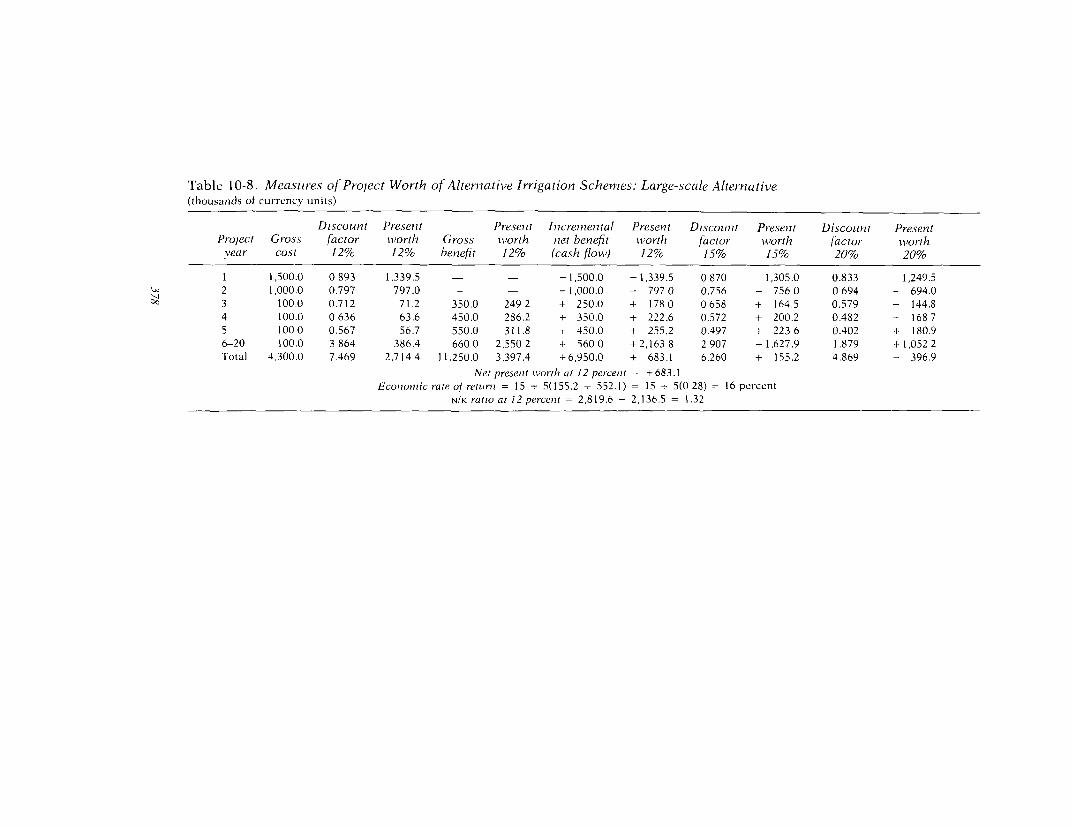
Table 10-8. Measltres of Project Worth of Alteniative Irrigationt Schemles: Large-scale Alternative(thousands of currency unils)
Discotint Present Presenit Incremental Present Discontii Presenzt Discount Presenit
Project Gross factor worth Gross worth niet benefit wvorth factor worth factor worth
year cost 12% 12% benefit 12% (cash flow) 12% 15% 15% 20% 20%
1 1,500.0 0 893 1,339.5 - - - 1,500.0 - 1,339.5 0 870 - 1,305.0 0.833 - 1,249.5
2 1,000.0 0.797 797.0 - - - 1,000.0 - 7970 0.756 - 756 0 0 694 - 694.0
3 100.0 0.712 71.2 350.0 249 2 + 250.0 + 178 0 0658 + 164.5 0.579 + 144.8
4 100.0 0 636 63.6 450.0 286.2 + 350.0 + 222.6 0.572 + 200.2 0.482 + 168 7
5 100 0 0.567 56.7 550.0 311.8 + 450.0 + 255.2 0.497 + 223 6 0.402 + 180.9
6-20 100.0 3 864 386.4 660 0 2,550 2 + 560 0 + 2,163 8 2907 + 1,627.9 1.879 + 1,0522
Total 4,300.0 7.469 2,714 4 11,250.0 3,397.4 + 6,950.0 + 683.1 6.260 + 155.2 4.869 - 396.9
Net preset wvorth at 12 percent = +683.1
Economic rate of rettrn = 15 + 5(155.2 - 552.1) = 15 4- 5(0 28) = 16 percent
N/K ratio at 12 percent = 2,819.6 - 2,136.5 - 1.32

APPLYING DISCOUNTED MEASURES OF PROJECT WORTH 379
benefit-investment ratio of 1.99, so we would select it over the largerproject, which has a net benefit-investment ratio of only 1.32. But weknow from the discussion of the application of the net present worthcriterion that this would be an erroneous choice because we would beforgoing the additional wealth the larger project could create. When weuse the internal rate of return criterion, we can avoid this error if wediscount the differences between the cash flows of the two projects as isdone in table 10-9. There we find that the internal rate of return to thestream of the differences is 14 percent. In other words, if we expand theproject from the smaller alternative to the larger, the return to ouradditional investment is 14 percent. The proper choice criterion, then, iswhether the return to our additional investment is above the cut-off rate.Since the cut-off rate in this example is taken to be 12 percent, the returnon the additional investment would still be above the cut-off, and wewould reject the smaller project in favor of the larger.
Different scales of a project
Sometimes we may wish to choose between a smaller version of aproject and a larger version of the same project. Such a case arose in aBrazilian forestry project. The smaller version of the project consistedsimply of cutting logs and exporting the round wood; it had a positive netpresent worth, quite a high economic rate of return, and an attractive netbenefit-investment ratio. A somewhat larger version of the project in-cluded a sawmill; it had a larger net present worth than the smallerversion, but a lower economic rate of return and a smaller net benefit-investment ratio. We could consider the larger version a mutually exclu-sive alternative to the smaller version.
Applying the net present worth criterion, we would correctly choosethe larger version. Note, however, that simply applying directly theeconomic rate of return or net benefit-investment ratio criterion wouldhave led to an erroneous investment decision.
In this case, undertaking the small project does not preempt the site.We can choose, if we wish, to undertake the small project and thenproceed to expand it. Under these circumstances, we do our analysis notof the small version versus the large version, as if the two were mutuallyexclusive projects, but of the small version as the first phase of a two-phase program. By the net present worth criterion, we know from ourearlier discussion that the smaller version, now called phase i, has apositive net present worth, so we would accept it. Then, if we tested theexpansion necessary to reach the larger version, now called phase ii, wewould find that this phase also has a positive net present worth, and sowe would accept it, too. If we wanted to use the internal rate of returnapproach, the economic rate of return of the second phase of the programwould be the economic rate of return of the differences between theincremental net benefit streams of the two versions. Similarly, the netbenefit-investment ratio of the phase-II project would be the net benefit-investment ratio of the differences of the incremental net benefit streams

Table 10-9. Meastires of Project lVorth of Alhernative Iwrigationi Schemies:Diff/re1ieces between Altern1atives(tiloLIsanicds of cuTr11CY Uni1ts)
Caohs f[lo' Cash flon'of of Differences Discotint Present Discouint Present
Project large-scale small-scale between fcactor worth factor wvorthyear scheme scheme caslh flow.s 12% 12% 15% 15%
I - 1,5000 - 5000 - 1,000.0 0 893 - 893.0 0.870 - 870.02 - 1,000 0 -,- 135 0 - 1,135 0 0.797 - 904.6 0.756 - 858.13 + 250 0 + 135 0 + 115 0 0.712 + 81.9 0.658 + 75.74 + 350 0 + 135.0 + 215.0 0.636 + 136.7 0.572 + 123.05 + 450(0 + 1350 + 315.0 0567 + 178.6 0497 + 156.66-20 + 560 0 + 135 0 + 425.0 3.864 + 1,642 2 2.907 + 1,235 5Total + 6,9500 +2,065.0 +4,8850 7.469 + 241.8 6.260 - 137.3
Net presenit wvorth at 12 percenit of the difterencesbetween incremental net benefit streatmts = + 241 8Economic rate of return of the dtff/rences betwteen
tncremnental niet benefit streams= 12 + 3(241 8 - 379.1) = 12 + 3(0 64) = 14 percent

APPLYING DISCOUNTED MEASURES OF PROJECT WORTH 381
of the two versions. Breaking a project down into phases is the moredirect approach and the more easily understood. Such an approachpermits us to apply any of our measures of project worth directly withoutfurther manipulation.
Of course, if we have sufficient administrative and other resources, wemay very well implement two phases-or even more-of a project simul-taneously. By analyzing each phase separately, we can tell directly fromour analysis how large the project can be before we reach a phase that hasa negative net present worth, an economic rate of return below ourcut-off rate, or a net benefit-investment ratio less than that of alternativeproject opportunities.
Different timing of a project
A special case of the choice among mutually exclusive projects is thequestion of whether to begin a project immediately or to postpone it. Thesame project begun today or at some future time may be considered,from an analytical standpoint, to be two different, mutually exclusiveprojects.
Postponing a project can be advantageous only if the potential benefitor cost stream will increase independently of when a project is begun. Inmost agricultural production projects, this is not the case. Rather, it isassumed that costs and benefits will come at some given period of timeafter the start of the project. If the project is postponed, both costs andbenefits will also be postponed and for the same period of time.
Questions of the best time to begin implementation can arise in agri-cultural projects when there is a processing facility to be constructed. Wemay want to establish sugar beets in a new area. We have an idea of themaximum rate at which we can expand the area for sugar beets given thelimitations imposed by extension work, rates at which farmers willadopt new practices, and the like. We have a choice between shipping thebeets to another area for processing-incurring both a transport cost anda loss of sucrose because of natural deterioration in the raw material-orbuilding a new factory of a minimum economic size. Here we have a casewhere timing should be assessed. The potential benefit of the projectgrows independently of the beet factory up to its capacity because thebenefit is dependent upon the rate at which farmers increase their outputof beets. In the first years of the project it might be too expensive toprovide for local processing, but at some point the savings in transportcost and sucrose loss will make it economic to build the factory. Theproblem is when is it most economic to begin.
There are two general approaches commonly employed to determinethe optimal time to begin a project. The simplest timing test to calculate,and probably the most widely used in practice, is the "first-year return"method. This technique makes an implicit assumption that once benefitsbegin they will be rising or constant, but this is the most commonsituation in all kinds of projects and so is not a serious drawback. In thistest, the net benefit stream in the first year the stream is positivc is

382 MEASURES OF PROJECT woRiri
divided by the total of the net benefit stream in those years it is negative.The result expressed in percentage terms is the first-year return. Theoptimal time to begin the project is the earliest year for which the netbenefit stream for a project begun in that year has a first-year returnexceeding the opportunity cost of capital. If the project begins earlier, forat least the first year it will fail to earn the opportunity cost of capital,and so it would be better to postpone implementation and use the moneyelsewhere. If the project begins later, a chance to earn the opportunitycost of capital on the initial investment will be passed by.
The second timing test, somewhat more difficult to calculate than thefirst-year return test but the easiest test to interpret, is to compute the netpresent worth of the project by assuming it will begin in different yearsand by discounting at the opportunity cost of capital. (The same year istaken as to for all of the alternative net present worth computations.) Theproject should begin in that year when the net present worth is thegreatest. Before that time, postponing the project will increase its netpresent worth at the given opportunity cost of capital; after that time, thenet present worth of the project will be less than it need be.
A very common instance of the need to determine optimal timingoccurs in relation to traffic growth in road projects. The application ofthe methods of determining the optimal time to begin a project can beillustrated by the Kenya feeder road example laid out in table 10-10. Thecost of constructing the road, divided equally between two years, isestimated at K£760.0 thousand. (The symbol for Kenyan pounds is K£.Since this analysis was made, the unit of currency used in budgeting inKenya has been changed from pounds to shillings, or KSh.) The road isassumed to have an economic life of thirty years. The earliest the projectcould have begun was 1970. Once the road was complete, there would bea two-year period while the traffic built up rapidly as people learnedabout the new road and new traffic was generated. After that, the trafficlevel would be determined by the general economic conditions of thearea and was assumed to grow by 9 percent a year until 1991 and to beconstant thereafter for the balance of the economic life of the road. Theincremental net benefit streams given in table 10-10 are based on thebenefit stream derived from the traffic estimates. (The traffic estimateswere made on the basis of growth over 20 years on the assumption thatthe road was begun in 1970. It will be seen that, even if traffic wereassumed to continue to grow after 1991, the optimal time to begin theproject would not change.) A residual value was assumed that was basedon linear depreciation in those cases where the benefit stream does notlast a full thirty years. An opportunity cost of capital of 12 percent isassumed.
To illustrate the first-year return method, we may consider the effect ofbeginning the road in 1973. The first year the net benefit stream ispositive, it amounts to K£79.7 thousand. This is only 10 percent of theinvestment cost (taken to be the sum of the negative values of the netpresent worth stream), an indication that it is too soon to begin theproject [79.7 . (380.0 + 380.0) x 100 = 10]. If we test for beginning the
APPLYING DISCOUNTED MEASURES OF PROJECT WORTH 383
road in 1974, the net benefit stream in the first year the net present worthis positive amounts to K£86.4, which is only 11 percent of the investment,and it is still too early to begin [86.4 - (380.0 + 380.0) x 100 = 11]. Butnow if we test for beginning the road in 1975, when the net benefit streamthe first year it is positive amounts to K£94.5 thousand, we find the firstyear return to be 12 percent [94.5 (380.0 + 380.0) x 100 = 12]. Since12 percent is our opportunity cost of capital, the first-year return methodindicates that 1975 is the optimal year to begin the project.
To determine the optimal time to begin the project using the netpresent worth method, the net present worth of the road was computedfor each timing alternative from 1970 through 1977. The calculation took1969 as to (that is, 1970 = tl). The net present worth reaches its greatestvalue of K£300.6 if the road were to be postponed five years and construc-tion begun in 1975. This, then, is the optimal timing alternative, a resultconsistent with that we obtained using the first-year return method.Beginning the road either before or after 1975 would result in a lower netpresent worth.
In this example of mutually exclusive timing alternatives, an invest-ment decision based only on a simple economic rate of return computa-tion would have led to an erroneous choice. Beginning the project in 1970would yield an overall economic rate of return from the project as awhole of 15 percent. Since this is well above the opportunity cost ofcapital, at first glance it might seem justifiable to proceed with theproject. But we know from our first-year return analysis that if theproject is begun in 1970 the return to the capital invested in the first yeara positive benefit is received is only 8 percent, and it would thus be betterto postpone the investment. Choosing the optimal starting year of 1975means that the project will have an economic rate of return of 19 percent.If we postpone the project still further, we know that the present worth ofthe project at the opportunity cost of capital falls-but note that thesimple economic rate of return to the project as a whole continues to rise,and this might be misleading to the unwary or ill-advised projectanalyst.
The internal rate of return criterion can be manipulated to indicate theoptimal timing by discounting the differences between the cash flows ineach succeeding year until the internal rate of return to the incrementalcash flow just equals the opportunity cost of capital. This calculation,however, is complex and more difficult to interpret than either thefirst-year return or the net present worth approach.
In the Kenya example, the net benefit-investment ratio also indicatesthe optimal timing directly, but since the net benefit-investment ratiocannot in general be relied on to choose between mutually exclusiveprojects, its use to determine optimal timing is inadvisable.
Choice between technologies (crossover discount rate)
When there are technological alternatives by which we can realize thesame result when designing a project, we have an instance of mutually

Table 10-10. Determiination of Optimal Timing. Third Highway Loan Project, Feeder Road Number 10, Kenya
(thousands of K£)
Incremiienital net benefit assuming construction to begin in:
Year 1970 1971 1972 1973 1974 1975 1976 1977
1970 - 380.0 - - - - -
1971 - 380.0 - 380.0 - - - - - -
1972 + 61.0 -380.0 -380.0 - - - - -
1973 + 69 1 + 67.0 -380.0 -380.0 - - - -
1974 + 77.7 + 75.3 + 73.0 - 380.0 - 380.0 - - -
1975 + 84.7 + 84 7 + 82 7 + 79.7 - 380.0 - 380.0 - -
1976 + 92 3 + 92.3 + 92.3 + 89.7 + 86.4 -380.0 -380.0 -
1977 + 100.6 + 100.6 + 100.6 + 100.6 + 97.8 + 94.5 -380.0 -380.0
1978 + 109.7 + 109.7 + 109.7 + 109.7 + 109.7 + 1069 + 102.6 -380.0
1979 +119.6 -+-119 6 +119.6 +119.6 +119.6 +119.6 +-116.0 +111.8
1980 + 130.3 + 130.3 + 130.3 + 130.3 + 130.3 + 130.3 + 130.3 + 126.4
1981 + 142 0 + 142.0 + 142.0 + 142.0 + 142.0 + 142.0 + 142.0 + 142.0
1982 + 154.8 + 154 8 + 154.8 + 154.8 + 154.8 + 154.8 + 154.8 + 154.8
1983 + 168.8 + 168.8 + 168.8 + 168.8 + 168.8 + 1688 + 168.8 + 168.8
1984 + 183.9 + 183.9 + 183.9 + 183.9 + 183.9 + 183.9 + 183.9 + 183.9
1985 +200.5 +200 5 + 200.5 + 200.5 +200.5 +200.5 +200.5 +200.5
1986 +218.5 +218.5 +218.5 +218.5 +218.5 +2185 +218.5 +218.5
1987 +238.2 +238.2 +238.2 +238.2 +238.2 +238.2 +238.2 +238.2

1988 +259.7 +259.7 +259.7 +259.7 +259.7 +259.7 +259.7 +259.71989 +283.0 +283.0 +283.0 +283.0 +283.0 +283.0 +283.0 +283.01990 +308.5 +308.5 +308.5 +308.5 +308.5 +308.5 +308.5 +308.51991-
2000 + 336.3 + 336.3 + 336.3 + 336.3 + 336.3 + 336.3 + 336.3 + 336.32001 + 336.3 + 361.6' + 3 8 6 .9 + 412.2c +4 3 7 .5 + 462.8' +488.I' + 5 1 3 .4gPresent
worthat 12percent +238.9 +262.2 +279.1 +290.8 +297.6 +300.6 +299.6 +295.4
First-yearreturn(percent) 8 9 10 10 11 12 14 15
Economicrate ofreturn(percent) 15 16 16 17 18 19 20 21
N/K ratio 1.31 1.35 1.37 1.38 1.39 1.40 1.39 1.39
Source: Adapted from World Bank, "Appraisal of a Third Highway Project, c. Includes residual value of K(75.9 thousand.Kenya," PTR-24a (Washington, D.C., 1969). Since this analysis was made, the d Includes residual value of Kf:101.2 thousand.unit of currency used in budgeting in Kenya has been changed from pounds to e. Includes residual value of K£126.5 thousand.shillings (KSh). f. Includes residual value of KE151.8 thousand
a. Includes residual value of K£25.3 thousand. g. Includes residual value of KE177.1 thousand.b. Includes residual value of K£50.6 thousand.

386 MEASURES OF PROJECT WORI'H
exclusive alternatives because the choice of one technology precludes theuse of another for the same purpose. The alternative we choose will be theone with the lower net present worth, but, if the total undiscounted costof using the different alternatives is different and they have differing timeprofiles, the alternative we choose may depend on the opportunity cost ofcapital.
Suppose we have a choice between two grain storage systems-onethat uses silos and bulk handling and that has the lower undiscountedcost, and the other that uses warehouses and bags. The bulk handlingsystem involves a high initial investment for silos but has low upkeep.The alternative system based on warehouses and bagging has a muchlower construction cost but will entail substantial annual operating cost.At a low discount rate, the silo system with its high initial cost but lowoperating cost will have the lower net present worth-thus it would bepreferred. At a high discount rate, however, the warehouse and baggingsystem with its low initial cost but high operating cost will have thelower net present worth. At some discount rate, both alternatives willhave the same net present worth, and we will be indifferent on economicgrounds which alternative we choose. This is known as the "crossover (orequalizing) discount rate," and it can be found either graphically or bydiscounting the differences between the cost streams. If the cost of capi-tal or cut-off rate is below the crossover discount rate, we will prefer thealternative that entails the higher initial capital outlay but lower ex-penditure in the future. Above the crossover discount rate, we will preferthe technological alternative with the lower initial cost, even though thisinvolves higher operating cost later.
We may illustrate this with a forestry project in Tunisia; the analysis islaid out in tables 10-1 1 through 10-13 and in figure 10-1. It was proposedto clear an area covered with maquis, a scrubby underbrush found in theMediterranean region, at the rate of 400 hectares a year for five years toprepare the ground for reforestation. Two technological alternatives
Table 10-11. Choice between Manual and Mechanical Land Clearingin Tunisia: Manual Clearing Alternative(US$)
Present PresentProject Other Total wvorth iworth
year Wagesa Costa cost 10% 15%
1 44,050 3,800 47,8502 44,050 3,800 47,8503 44,050 3,800 47,850 181,399 160,3934 44,050 3,800 47,8505 44,050 3,800 47,850Total 220,250 19,000 239,250 181,399 160,393
US$ U.S. dollars.Source: Personal communication from Mr. Hans Warvinge, Swedish International De-
velopment Authority (December 1971).a. All values at market prices.

APPLYING DISCOUNTED MEASURES OF PROJECT WORTH 387
Table 10-12. Choice between Manual and Mechanical Land Clearingin Tunisia: Mechanical Clearing Alternative(US$)
Operation Present Presen tProject Equipment and Total worth worthyear cost' maintenancea cost 10% 15%
1 90,700b 21,586 112,286 102,068 97,6892 0 25,134 25,134 20,761 19,0013 0 25,134 25,134 18,876 16,5384 0 26,227 26,227 17,913 15,0025 0 26,227 26,227 16,287 13,035Total 90,700 124,308 215,008 175,905 161,265
Source: Same as table 10- 11.a. All values at market pricesb. Tractor and clearer c.i.f. Tunis, taxes included.
were available. The land could be cleared manually at a cost ofUS$47,850 per year spread evenly over the five-year period for an undis-counted total cost of US$239,250 (table 10-1 1). Alternatively, tractorsand clearing equipment could be purchased and the area cleared me-chanically at a lower undiscounted total cost of US$215,008 (table 10-12). The mechanical clearing alternative involved a large initial capitalexpenditure of US$90,700; after that, however, operation and mainte-nance costs would only be some US$25,000 a year.
The proper choice between these two alternatives must allow for thetime value of money. If a discount rate of 10 percent is assumed, we findthe mechanical alternative continues to be cheaper and has the lowerpresent worth. At 15 percent, however, we find the manual method hasthe lower present worth and, hence, costs less. If we subtract year by yearthe cost stream of the cheaper undiscounted alternative (in this case, themechanical clearing) from the more expensive undiscounted alternative(the manual clearing) and then find the discount rate that brings thestream of the differences between the cost streams to zero, we will findthat discount rate at which the present worths of the two alternatives areequal (hence, the term "equalizing discount rate"). From an economicstandpoint, at this rate we are indifferent about the alternatives. Asshown in table 10- 13 for the Tunisian example, this crossover or equaliz-ing discount rate is 14 percent. (This discount rate may also be derivedgraphically as illustrated in figure 10-1.) If our opportunity cost of capitalwere 10 percent, we would prefer the mechanical clearing alternative,assuming that our criteria were based strictly on cost grounds. If theopportunity cost of capital were 15 percent, we would prefer the manualclearing alternative, even though this is the more expensive alternativein absolute (undiscounted) terms. If the opportunity cost of capital were14 percent, on economic grounds we would be indifferent about thealternatives.
In Tunisia, where the opportunity cost of capital was probably notmuch, if any, less than 14 percent, the manual alternative would doubt-

388 MEASURES OF PROJECT WORTH
Table 10-13. Choice between Manual and Mechanical Land-clearingAlternatives in Tunisia: Crossover Discount Rate(US$)
Differences Present PresentProject between worth worthyear cost streams 10% 15%
1 - 64,436 - 58,572 - 56,0592 +22,716 + 18,763 + 17,1733 +22,716 + 17,060 + 14,9474 +21,623 + 14,769 + 12,3685 +21,623 + 13,428 + 10,747Total + 24,242 + 5,448 - 824
Crossover discount rate = 10 + 5[5,448 - (5,448 + 824)] = 10 + 5(0.87) = 14 percent
Source: Same as table 10- 11.
lessly be chosen if for no other reason than the employment effect manualclearing would have. Note, too, that the example uses market prices. Ifwe were to shadow-price labor at 50 percent of its wage, the undis-counted cost of the manual clearing alternative falls to US$129,125[(220,250 x 0.50) + 19,000 = 129,125], which makes it well below theundiscounted cost of the mechanical alternative even if we reduce thecost of the tractor and clearing equipment by the amount of duties andtaxes. At the shadow wage, there would be no case at all for the mechani-cal alternative in this example. In other projects, however, the effect ofthe shadow wage would be to reduce the crossover discount rate-possibly to move it below a cut-off rate so that a labor-intensive alterna-tive that would not be attractive at market prices might prove to be thepreferable alternative if shadow prices were used in the economicanalysis.
This Tunisian example shows vividly how low (perhaps subsidized)interest rates and high wages (perhaps the result of minimum wageregulations) can encourage mechanization and reduce employment.
Additional purposes in multipurpose projects
A variation of the problem of mutually exclusive alternatives arises inmultipurpose projects. In these, a project design that includes one groupof purposes is a mutually exclusive alternative to another project designthat includes a different group of purposes. The problem is frequentlymet in rural development projects, and another common example isfound in river basin development projects.
The reason we are interested in multipurpose projects, of course, isthat often it is possible to provide a group of related goods and servicesmore cheaply from a single project than it is to provide the same benefitsfrom the most economic, alternative single-purpose projects. But there isa danger that a very beneficial purpose (flood control, perhaps) may driveup the overall economic rate of return and thus hide another purpose(irrigation, perhaps) that should be omitted.

APPLYING DISCOUNTED MEASURES OF PROJECT WORTH 389
Figure 10-1. Graphic Derivation of Crossover Discount Rate,Choice between Mechanical and Manual Land-clearingAlternatives in Tunisia
I 85
180 _
Manual\\ / clearing
alternative
-E 175
0
170- Mechanical/ clearing_
alternative
165-
CIrossovrdiscount rate
160 l_______l_______________I___________
Discount rate(percent)
Source: Table 10-5.
Projects may conveniently be tested for the desirability of an addi-tional purpose by determining the net present worth of the alternativegroups of purposes at the opportunity cost of capital. If the project has agreater net present worth with an additional purpose than without it,then the additional purpose is justified. But if the net present worth isreduced by including an additional purpose, then obviously it would beundesirable to include the additional purpose in the project.
The method of analysis is illustrated in tables 10-14 through 10-16. Amultipurpose river basin project can be built to provide only flood con-trol and power benefits, or it can be expanded to include an irrigationcomponent. The separable cost wholly attributable to each purpose isgiven in the first part of table 10-14. These indicate the extent to whichthe cost of the project would be reduced were one component omitted. Inthis instance, omitting irrigation reduces the cost of the project byUS$ 18,965 thousand. The alternative cost of providing each benefit in theproject by means of the most economic alternative single-purpose proj-

390 MEASURES OF P'ROJECT WORTH
Tablc 10-14. Separable and Alternative Costs,Multipurpose River Basin Project, United States(thousands of US$)
Project Flood Irriga-year control tion Powver
Separable cost1 84 1,132 6002 1,244 1,970 1,5303 907 2,865 2,0854-100 5 134 61Total 2,720 18,965 10,132
Alternative cost
1 2,380 1,880 7152 4,740 5,270 2,1003 1,370 2,565 1,4954-100 22 220 226Total 10,624 31,055 26,232
Source: Adapted f-omi U S. Government, Department of the Interior, Bureau of Reclama-tion, Reclamation Instruction Series 110, Prolect Plannizntg (Washington, D.C., 1959),p. 116.5.19.
ect is given in the second part of table 10-14. If the present worth ofproviding the same purpose by a single-purpose alternative were lessthan the present worth of the separable cost for providing that samepurpose in the multipurpose project, there would be no grounds forincluding that purpose in the multipurpose project. In table 10-15, dis-counting at 2.5 percent (the rate in use at the time this analysis was done)shows that the net present worth of the project increases from US$8,273thousand to US$10,935 thousand when the irrigation component isadded. The investment decision, then, would be to include the irrigationcomponent in the project. Had the net present worth with irrigation beenless than US$8,273 thousand, the investment decision would have beento omit the irrigation component.
The same investment decision would have been reached if the methodof discounting the differences between the cash flows had been used,although this involves more calculation and more chance of error. Thisapproach is illustrated in table 10-16. There the economic rate of returnto the irrigation component is found to be 4 percent. Since this is greaterthan the opportunity cost of capital or cut-off rate of 2.5 percent, theinvestment decision would be to accept the irrigation component. Note,however, that if one were simply to calculate an internal rate of return forthe two versions of the project, with irrigation and without irrigation, theversion without irrigation has a slightly higher internal rate of return. Ifone were not careful about the method of analysis using the internal rateof return for mutually exclusive projects, the wrong investment decisionmight be made. (Note the relation between the net present worth analy-sis in table 10-15 and the analysis discounting the differences betweencash flows in table 10-16. The differences of the net present worths of thecash flows discounted at 2.5 percent in table 10-15 is US$2,662 thousand

APPLYING DISCOUNTEI) MEASURES OF PROJECT WORTH 391
Table 10-15. Measures of Project Worth without an1d with Irrigation,U.S. Multipurpose River Basin Project(thousands of US$)
Benefit Incremental Discotunzt Present
Project Flood Inriga- net benefit factor wvor1thyear Cost control tion Powver (cash flowv) 2.5% 2.5%
Withiotut irrigation1 2,456 - - - 2,456 0.976 - 2,3972 6,218 - - - - 6,218 0.952 - 5,9203 1,983 - - - - 1,983 0.929 - 1,8424-100 72 271 - 347' 546 33 758 + 18,432Total 17,641 26,287 - 33,659 +42,305 36.615 + 8,273
Net presenit worth at 2.5 percenzt without irrigation = US$+8,273Intenial rate of retunl tvithout irrigation = 4.8 percentb
N/K ratio at 2.5 percent without irrigationi = US$18,432 - US$10,159 = 1.81b
With irrigation1 3,588 - - - - 3,588 0.976 - 3,5022 8,188 - - - - 8,188 0.952 - 7,7953 4,848 - - - - 4,848 0.929 - 4,5044-100 206 271 380 347' + 792 33.758 +-26,736Total 36,606 26,287 36,860 33,659 60,200 36.615 + 10,935
Net present worth at 2.5 percent with irrigation = US$+ 10,935Internal rate of returni with irrigation = 4.5 percentb
N/K ratio at 2.5 percent with irrigation = US$26,736 -- US$15,801 = 1.69b
Source: Same as table 10-14.a. See the text for a discussion about valuing the powver benefit.b. See the text for a discussion about interpreting these measures.
(10,935 - 8,273 = 2,662), which is exactly the net present worth of thedifferences of the streams of cash flows discounted at 2.5 percent asshown in table 10-16.)
For illustrative purposes, the net benefit-investment ratio has beenincluded in table 10-15. Note that the net benefit-investment ratio with-out irrigation, 1.81, is larger than the net benefit-investment ratio withirrigation, 1.69. Once again we find that the net benefit-investment ratiocannot be relied on to choose between mutually exclusive alternatives.
A complication arises in regard to the benefit of the power component.The economic benefit of electricity is generally considered not possible toestimate. What is the benefit of electricity, especially if much of it goes forhousehold use? In economic analysis of single-purpose projects, thisdifficulty is usually resolved by assuming that alternative projects gener-ating the same amount of electricity will have an equivalent benefit andby simply choosing the one for which the present worth of the cost islowest. In analyzing projects such as this multipurpose one, however, adifferent approach to valuing power is conveniently adopted. It may beassumed that if power consumers are willing to pay the price that wouldhave to be charged to provide the same amount of electricity by the mosteconomic single purpose as indicated in the second part of table 10-14,then the economic value of the power component in the multipurpose

Table 10-16. Discounting Differences betiveen Cash Flows, With and WithotitIrrigation, U.S. Multipurpose River Basin Project(thousands of US$)
Incremnental Incrementalnet benefit net benefit(cash flow) (cash flow) Differences Discount Present Discount Present
Project wvith without betwveeni factor wvorth factor worthyear trrigation irrtgatton cash flows 2.5% 2.5% 5% 5%
1 - 3,588 - 2,456 - 1,132 0.976 - 1,105 0.952 - 1,0782 - 8,188 - 6,218 - 1,970 0.952 -1,875 0.907 - 1,7873 - 4,848 - 1,983 - 2,865 0.929 - 2,662 0.864 - 2,4754-100 + 792 + 546 + 2461 33.758 +8,304 17.125 +-4,213Total +60,200 +42,305 + 17,895 36 615 + 2,662 19.848 - 1,127
Intenzal rate of return of irrigation component = 2.5 + 2.5(2,662 - 3,789) = 4 percentb
Source: Same as table 10-14.a. See the text for a discussion about valuing the power benefitb. See the text for a discussion about interpreting this measure.

APPLYING DISCOUNTED MEASURES OF PROJECT WORTH 393
project is at least that much. That being the case, we may take the annualbenefit of the power to be at least the annual equivalent of the net presentworth of the cost of providing the power by means of the most economicsingle-purpose alternative.
In this instance, if we discount the stream of costs for the most eco-nomic single-purpose power alternative as given in the second part oftable 10-14 at the opportunity cost of capital of 2.5 percent, we reach anet present worth of US$11,715 thousand. To convert this net presentworth to an annual equivalent, we need the capital recovery factor for theperiod from the 4th through the 100th year of the project, since powerfrom the single-purpose alternative is assumed to begin to flow in the 4thyear. This cannot be determined conveniently from a commonly used setof compounding and discounting tables such as those in Gittinger (1973).We can, however, calculate the capital recovery factor directly by deter-mining the present worth of an annuity factor for the 4th through the100th years and by then taking the reciprocal of that, since the capitalrecovery factor is the reciprocal of the present worth of an annuity factor.(This method is discussed in more detail in the section on "Joint CostAllocation" in chapter 6.) The present worth of an annuity factor at 2.5percent for 100 years is 36.614 105. This may be obtained from a detailedset of compounding tables, from calculation along the lines of the discus-sion in the last section of this chapter, or from the formula in appendix B.The present worth of an annuity factor for 2.5 percent for 3 years is 2.856024, so that the present worth of an annuity factor at 2.5 percent for the4th through the 100th years is 33.758 081 (36.614 105 - 2.856 024 =33.758 081). The capital recovery factor for the 4th through the 100thyears at 2.5 percent can then be obtained by taking the reciprocal of thepresent worth of an annuity factor, or 0.029 623 (1 + 33.758 081 = 0.029623). We then apply that factor to the net present worth at 2.5 percent ofthe stream of costs of providing the power by the most economic single-purpose alternative, US$11,715. The result is the annual value of the costof providing the power by the single-purpose alternative, US$347thousand (11,715 x 0.029 623 = 347). This value can then be used toestimate the present worth of the multipurpose project with and withoutthe irrigation component. A fuller discussion of valuing electricity will befound in van der Tak (1969).
Applying Contingency Allowances
For many estimates of project costs, especially costs of those projects inwhich there is a considerable element of construction in the earlier years,the engineers will often include a contingency allowance. We noted inchapter 2 that physical contingency allowances and contingency allow-ances intended to reflect relative price changes are real costs in bothfinancial and economic analysis and should be incorporated directly intothe project accounts even when the analyst is working in constant prices.
The contingency allowance intended to allow for general inflation,

394 MEASURES OF PROJECT WORTH
however, does not enter into the project accounts, either financial oreconomic, when the analyst is working in constant prices. This meansthat when inflation is expected to be significant, a separate financingplan will be needed to give those responsible for making budget alloca-tions a better idea of the amounts in current terms that they will be askedto make available.
Because future price increases can affect costs only until work is com-pleted, the overall contingency allowance for inflation is built up byapplying the appropriate compounding factors to the amount to beexpended each year. Suppose we take a project with an expected totalcost of US$390 thousand in constant terms as of the beginning of theproject, or to. Construction costs are to be incurred equally each year overa three-year construction period. We expect inflation to be 8 percent ayear during construction. We can lay out the computation as follows(costs are in thousands of U.S. dollars):
Project cost Compounding Project costin constant factor for I in current
Year terms at 8 percent terms
1 130 x 1 080 = 1402 130 x 1.166 = 1523 130 x 1.260 164Total 390 456
The total cost for the project in current terms would thus be US$456thousand, and the price contingency would be 17 percent [(456 - 390) +390 x 100 = 17]. This, of course, is quite different from the 26 percentprice contingency we would obtain if we were to compound the wholeproject cost in constant terms over the three-year period [390 x 1.260 =
491; (491 - 390) . 390 x 100 = 26].Contingency allowances are usually not included for the operating
costs of a project once the initial investment stage is passed. Rather,problems such as higher than anticipated production expenditures arecustomarily analyzed by using sensitivity analysis, and a judgment isthen made about whether to change the design of the project or toabandon it.
In agricultural credit projects, it is generally not necessary to includecontingency allowances. Changes in unit costs for this kind of project willprimarily affect the number of loans that can be made with the fundsavailable rather than the economic justification of the project itself.Contingencies in agricultural credit projects usually will, however, betreated in the discussion of the economic justification of the project,perhaps in conjunction with the sensitivity analysis.
Contingency allowances are best shown separately in project tables,with appropriate explanations of how they were calculated included inthe accompanying text and notes. To avoid double counting, any contin-gency allowances already included in the basic material used to preparethe project analysis should be eliminated. The amount of contingencyprovision will vary with the nature of the project and the general compo-nents of the project. Contingency allowances should be determined item

APPLYING DISCOUNTI ED MEASURES OF PROJECT WORTH 395
by item for each project, not based on some national standard allowance.In general, contingency allowances should not be large enough to coveralmost any cost overrun, since the possibility of so large a change occur-ring is small. Such excessive prudence will reduce the pressure for care-ful cost estimation, relax pressure for tight cost control during projectexecution, and result in misleading underestimates of the net presentworth, the financial and economic return, or the net benefit-investmentratio.
Physical contingency allowances usually are estimated separately foreach major category of cost and separately for local and foreign exchangecosts. Projects that include large civil engineering works require highercontingency allowances than projects that cover only the supply anderection of equipment. The cost of engineering works will be influencedby such factors as the topography and geology of the project area, theamount of field work necessary to prepare the detailed designs, unfore-seen technical difficulties (especially if the project involves subsurfacework), the risk of underestimating the amount of work actually required,changes in design during construction, and unusually bad weather thatmay interrupt work. If large amounts of equipment are involved, con-tingencies may be appropriate to allow for errors in estimating the exactamount'of equipment and the quantity of spare parts needed.
Contingency allowances for relative price changes during the earlyinvestment phase of a project may reflect anticipated influences arisingfrom domestic price increases, the expected trend of prices in leadingsupplier countries, price trends for particular kinds of work or kinds ofequipment to be used, and the possible effect of the project in exerting astrong upward pull on prices of locally supplied labor and raw materials.[A projected index of international inflation is included in Price Prospectsfor Major Primary Commodities (World Bank 1982a), which may be help-ful in estimating price trends in supplier countries and for importedequipment.]
Replacement costs
Many agricultural projects require investments that have differentlifetimes. A good example is found in the case of a pump irrigationscheme in which the earthworks and pump platforms may be expected tolast twenty-five to fifty years but the pumps themselves may have a life ofonly seven to fifteen years. In preparing the analysis, allowance must bemade for the replacement cost of the pumps during the life of the project.
Treatment of replacement costs is simple. The analyst includes themamong the capital items for the appropriate year in the project analysis.In analysis of the net present worth, internal rate of return, and netbenefit-investment ratio, the replacement costs are then netted out whenthe cash flow is computed. This may make the cash flow for that particu-lar year negative, but only rarely in an agricultural project could thisintroduce analytical complications (see the subsection on "More thanone possible internal rate of return" in chapter 9).

Table 10-17. Treatment of Replacement Cost, Lift Irrigation Project, India(thousand of Rs)
Invest- Incre- Incremental Discount Present Discount Present Discount PresentProject ment mnental net benefit factor ivorth factor worth factor ivorth
year cost benefit' (cash flowv) 12% 12% 30% 30% 35% 35%
1 469 0 - 469 0 893 - 419 0.769 -361 0.741 -348
2 223 0 - 223 0.797 - 178 0.592 - 132 0.549 - 122
3 0 155 + 155 0.712 + 110 0.455 + 71 0 406 + 63
4-8 0 310 + 310 2.566 + 795 1.109 +-344 0.902 +2809 223" 310 + 87 0 361 + 31 0.094 + 8 0.067 + 6
10-15 0 310 + 310 1.483 + 460 0.249 + 77 0.160 + 50
16 2 2 3 b 310 + 87 0.163 + 14 0.015 + 1 0.008 + I
17-22 0 310 + 310 0.671 + 208 0.040 + 12 0019 + 6
23 2 2 3 b 310 + 87 0.074 + 6 0.002 0 0.001 0
24 0 310 + 310 0.066 + 20 0.002 + 1 0.001 025 0 469, + 469 0.059 + 28 0.001 0 0.001 0
Total 1,361 7,134 + 5,773 7.845 + 1,075 3.328 + 21 2.855 - 64
Net presenit worth at 12 percenit = Rs+ 1,075Fi,naocial rate of return = 30 + 5[21 - (21 + 64)] = 30 + 5(0.25) = 31 percent
N/K ratio = Rsl,672 - Rs597 = 2.80
Rs Indian rupees. maintenance of the scheme are recovered by charges to farmers and are
Source: Adapted from "Report on Lift Irrigation Project in Sangli District, deducted from gross output as a production cost.
Maharashtra,' section 18 of Selected Agricultural Project Reports (Pune, Maha- b. Pump replacement.rashtra: College of Agricultural Banking, 1978), pp. 373-92. c. Includes residual value for pumps of Rsl59 thousand; civil works are
a. The incremental benefit is aggregated from farm budgets. Operation and assumed to have no residual value.

APPLYING DISCOUNTED MEASURES OF PROJECT WORTH 397
The treatment of replacement costs is illustrated in table 10-17. Theproject is a lift irrigation scheme proposed for Sangli District in the stateof Maharashtra in western India. The scheme would draw water from theKrishna River to serve three villages and would enable the farmers togrow hybrid sorghum, wheat, and sugarcane in addition to their tradi-tional, rainfed crops. The project would take two years to complete. Oncein operation, the civil works associated with the pumps could be ex-pected to last at least twenty-five years. The pumps themselves, however,are expected to be replaced every seven years. In table 10-17, the invest-ment column shows Rs223 thousand for pump replacement in years 9,16, and 23. The project thus allows for pump replacement quite directlyby simply including replacement as an investment cost in the years it isexpected to occur. (Note that there is a "residual" value to allow for theunexpired life of the last pump cycle in year 25; we will return to this inthe next subsection.) In this Indian example (as is generally the case), theinvestment cost for pump replacement is not large enough to turn thecash flow negative in any year when new pumps are to be installed, sothere is no possibility that there will be more than one solution when theinternal rate of return is calculated.
Residual value
Often at the end of a project there may reasonably be expected to besome residual (or terminal) value. That is, the capital asset will not havebeen all used up in the course of the project period, and there will be a"residual asset." The way to handle this is to treat the residual value ofany capital item (say a dam or a stand of trees) as a project "benefit"during the last year of the analysis period.
An example of a residual value is found in the analysis of the Indianpump project outlined in table 10-17 and discussed in the previoussubsection on replacement costs. The pumps in this project are replacedevery seven years. The last pump replacement before the end of theproject in year 25 occurs at the end of year 23. The pump, therefore, isexpected to have been used for only two years of its seven-year life by theend of the project. The value of the remaining useful life of the pumpshould not properly be charged as an investment cost to the project;instead, the project should be credited with the residual value in the finalyear of the project. Thus, in this example the analyst added an amountequal to five-sevenths of the Rs223 thousand investment cost included inyear 23 to the incremental benefit in year 25, or Rs 159 thousand [(7 - 2). 7 x 223 = 159].
On the whole, residual values will not change the net present worth,rate of return, or net benefit-investment ratio significantly unless theperiod of the analysis is short or the value of the capital items is quitelarge in relation to the value of the benefit stream. Such might be thecase, for instance, in a livestock project in which a very large residualvalue may build up in the form of a valuable herd. For agriculturalprojects carried out to 25 years or so, however, the residual value will

398 MEASURES OF PROJECT WORIll
usually not change the net present worth or the net benefit-investmentratio by more than a very small proportion, or the rate of return by asmuch as a percentage point. The reasons are the same ones noted in thediscussion of the length of the project period. At the earning capacities ofthe kinds of projects we are considering, the present worth of futurebenefits (hence, the present worth of residual values) is just not verygreat. A practical result of this is that projects are quite insensitive toerrors in estimating residual values. A rather gross estimate in a twenty-five-year project is adequate. Note that in table 10-17 virtually no error inestimating the salvage value could significantly affect the measures ofproject worth. Including residual values in the project analysis willforestall criticisms of the project analysis, or attempts to discredit aproject with a low initial investment in favor of another with a highinitial investment on the grounds that the analyst ignored the residualvalue. This may be important when discussing irrigation projects orlivestock projects because the technicians' concern and attention may belargely focused on the problems associated with the capital investmentin the dam or in the buildup of the breeding herd.
Domestic resource cost
In countries where there are balance of payments problems and whereimport substitution or export promotion is an important objective, it isuseful to estimate the cost in the domestic currency required to earn aunit of foreign exchange through a proposed project. The usefulness ofdoing so might arise, for instance, in preparing an oil palm project inwhich export or avoidance of vegetable oil imports is the objective or inevaluating a fertilizer plant intended to reduce or avoid future increasesin imports. It is not enough just to earn or save foreign exchange. Someidea must be formed of the cost of saving foreign exchange, and a judg-ment must be made about whether that cost is too high. By expressingthe cost of earning or saving a unit of foreign exchange as domesticresource cost, a direct comparison may be made with the official ex-change rate and various shadow prices for foreign exchange. Such acomparison is one basis for evaluating a project.
There are many approaches to estimating the domestic resource costand numerous theoretical problems to be resolved. These have beendiscussed at length by Bruno (1967), whose name is so closely identifiedwith this topic that the domestic resource cost is often called the Brunoratio.
Tables 10-18 and 10-19 illustrate a straightforward approach to esti-mating the domestic resource cost. This approach is suitable for mostproject purposes. Its major limitations are the tendency for some"domestic" costs to involve imports-the import consumption of work-ers, for example-and the partial analysis problem that is common to alldiscounted measures of project worth. Its advantages are its simplicityand the ease with which the result may be interpreted. To calculate thedomestic resource cost by this method, it is necessary to know four items:

APPLYING DISCOUNTEI) MEASURES OF PROJECT WORTH 399
Table 10-18. Calculation of Domestic Resource Cost,Indian Farmers Fertilizer Cooperative Fertilizer Project,India: Foreign Exchange Component(millions of US$)
Value of Invest- Produc- Other Incre- Discount Presentproduc- ment tion cost or mental factor worth
Year tion cost cost savinga saving 12% 12%
1970 - 7 - - - 7 0.893 - 61971 - 15 - - - 15 0.797 - 121972 - 15 - - - 15 0.712 - 111973 12 - 12 - 0 0.636 01974 38 - 18 - + 20 0.567 +111975 43 - 20 - + 23 0.507 + 121976 56 - 26 - + 30 0.452 + 141977 56 - 25 - + 31 0.404 + 131978 56 - 25 - + 31 0.361 +111979-84 56 - 25 - + 31 1.483 +46Total 597 37 276 - +284 6.812 +78
Source: Adapted from U.S. Government, U.S. Agency for International Development(USAID), "India: IFFCO Fertilizer Project Proposal and Recommendations for the Review ofthe Development Loan Committee," AID-DLC/P-851 (Washington, D.C., 1969), annexes 4Aand 4B.
a. If applicable, would include such differences in cost or saving as foreign exchange forinsurance, domestic currency saving in distribution from avoiding port charges and locat-ing production closer to the point of use, and the like.
Table 10-19. Calculation of Domestic Resource Cost,India Fertilizer Project: Domestic Currency Component(millions of Rs)
Invest- Produc- Other Incre- Discount Presentment tion cost or mental factor iworth
Year cost cost savings cost 12% 12%
1970 107 - - 107 0.893 961971 172 - - 172 0.797 1371972 56 - - 56 0.712 401973 24 38 - 62 0.636 391974 - 81 - 81 0.567 461975 - 90 - 90 0.507 461976 - 109 - 109 0.452 491977 - 109 - 109 0.404 441978 - 109 - 109 0.361 391979-84 - 108 - 108 1.483 160Total 359 1,184 - 1,543 6.812 696
Domestic Present worth of domestic currency costresource = of realizing foreign exchange saving Rs696 - US$78 = 8.92cost Present worth of net foreign exchange
savingb
Source: Same as table 10-18.a. If applicable, would include such differences in cost or saving as foreign exchange for
insurance, domestic currency saving in distribution from avoiding port charges and locat-ing production closer to the point of use, and the like.
b. From table 10-18.

400 MEASURES OF PROJECT WORTH
(1) the foreign exchange value of the product to be produced; (2) theforeign exchange cost incurred to produce the product (that is, the for-eign exchange cost of such things as imported fuels, imported raw mate-rials, and the like); (3) the domestic currency cost of producing theoutput; and (4) the opportunity cost of capital. The present worth of thenet foreign exchange benefit (discounted at the opportunity cost of capi-tal) is compared with the present worth of the domestic cost of realizingthese savings. The ratio between the two present worths is the domesticresource cost, and it may be directly compared with the official exchangerate or with shadow exchange rates.
The Indian Farmers Fertilizer Cooperative, Ltd., proposed to build amodern petrochemical fertilizer facility in the state of Gujarat. Theeconomic analysis gives the costs and benefits broken down into theirforeign exchange (table 10-18) and domestic currency (table 10-19) com-ponents. The domestic resource cost with a 12 percent opportunity costof capital assumed is Rs8.92 = US$1.
Since the official exchange rate at the time of the analysis was Rs7.50US$1, if the official exchange r ate is accepted as a true measure of the
value of the rupee (and 12 percent is accepted as the opportunity cost ofcapital), then it would cost more to manufacture through the project adollar's worth of fertilizer for import substitution than it would to buythe fertilizer from abroad. At the time the analysis was undertaken,however, it was widely considered in India that a foreign exchangepremium of at least 25 percent would better reflect the true value of therupee. This would make the shadow exchange rate Rs9.375 = US$1 (7.50x 1.25 = 9.375). If this rate is accepted (with 12 percent still the oppor-tunity cost of capital), then it would cost less to produce a dollar's worthof fertilizer than to import it because the domestic resource cost of Rs8.92= US$1 is a more favorable exchange rate than the shadow exchangerate of Rs9.375 = US$1.
Calculating Measures of Project WorthUsing Current Prices
We have often noted that project analyses are usually done at constantprices because the analyst is concerned with the real return to the projectwhen he is looking at the financial analysis and with the real, not mone-tary, effects of the project when he turns to economic analysis. Thus, it iscommon practice for the analyst to assume that general inflation willexert the same relative effect on both costs and benefits and to work inconstant prices.
Projects can, of course, be analyzed using current prices. If that weredone, general inflation would not affect the selection of projects providedthat all projects were analyzed using the same assumptions. That is, thesame group of projects would be accepted whether the analysis is done ona constant price basis or on a current price basis. Working with constant

APPLYING DISCOUNTED MEASURES OF PROJECT WORTH 401
prices, however, is the analytically simpler approach because it avoidsestimating a rate of inflation and simplifies the computations.
If we use net present worth as the measure of project worth, theamount of the net present worth will be different depending on whetherwe use current or constant prices (and also on whether we use a shadowforeign exchange rate or a conversion factor to allow for the foreignexchange premium). If we estimate the opportunity cost of capital for theanalysis correctly, we will still select the same group of projects toimplement. The opportunity cost of capital, however, will be higher byan allowance for inflation. If we use net present worth, we may assume adifferent rate for inflation for each year if that suits our analytical pur-pose. There is no easy means to compare the net present worth at currentprices to the net present worth at constant prices; the present worthcomputation must be repeated for each stream of values, and all projectsbeing analyzed must use the same assumptions. A similar commentholds for the net benefit-investment ratio. The value of the ratio willchange with changing assumptions about inflation and there is no easyway to compare the net benefit-investment ratio at current prices to thenet benefit-investment ratio at constant prices.
In contrast, an internal rate of return calculated at current prices, witha uniform general inflation rate assumed, can easily be converted to therate of return at constant prices by dividing 1 plus the internal rate ofreturn stated in decimal terms for the current prices by I plus the rate ofinflation stated in decimal terms. This is illustrated in table 10-20 withthe figures from the Ilocos, Philippines irrigation project that were givenin table 9-11. If we assume constant prices, the economic rate of return is18 percent. If we assume a uniform inflation rate of 6 percent throughoutthe life of the project, then we can derive the incremental net benefit(cash flow) in current prices for any given year by multiplying the in-cremental net benefit (cash flow) in constant prices for that year by theappropriate compounding factor for I at 6 percent. If we determine theinternal rate of return for the resulting incremental net benefit (cashflow) stream, we find it to be 25 percent. Dividing this result (in the formof I plus the internal rate of return stated in decimal terms) by theassumed inflation rate (also stated in the form of I plus the inflation ratestated in decimal terms) gives 1. 18-or the economic rate of return of 18percent we found using constant prices (1.25 . 1.06 = 1.18).
Calculator Applications in Project Analysis
We noted earlier that calculations for project analysis are simply tootedious to be done by hand; however, even the simplest electronic calcu-lators readily available in virtually every nation are sufficient for nearlyall calculations needed in project analysis. Indeed, they are the basiccomputational aid used both by national planning agencies and by inter-national lending institutions. Unfortunately, many project analysts do

Table 10-20. Internal Rate of Return Computation Using Current Prices,Ilocos Irrigation Systems Improvement Project, Philippines(millions of US$)
Incremental Com- Incrementalnet benefit pounding net benefit(cash flow) Discount Present factor (cash flow) Discount Present Discount Present
Project at constant factor worth for I at current factor ivorth factor worthyear pricesa 18%a l8%W at 6% pricesb 25% 25% 30% 30%
1 - 1.09 0.847 - 0.92 1.060 - 1.16 0.800 - 0.93 0.769 - 0.892 - 4.83 0.718 -3.47 1124 - 5.43 0.640 -3.48 0.592 -3.213 - 5.68 0.609 - 3.46 1.191 - 6.76 0.512 - 3.46 0.455 - 3.084 - 4.50 0.516 -2.32 1.262 - 5.68 0.410 -2.33 0.350 - 1.995 - 1.99 0.437 - 087 1.338 - 2.66 0.328 - 0.87 0.269 - 0.726 + 1.00 0.370 +0.37 1 419 + 1.42 0.262 +0.37 0.207 + 0.297 + 2.37 0.314 +0.74 1.504 + 3.56 0.210 +0.75 0.159 +0.578 + 3.70 0.266 +0.98 1.594 + 5.90 0.168 +0.99 0.123 +0.739 + 5 06 0.225 + 1.14 1.689 + 8.55 0.134 + 1.15 0.094 +0.80
10 + 6.43 0.191 +1.23 1.791 + 11.52 0.107 +1.23 0.073 +0.8411 + 6.43 0.162 + 1.04 1 .898 + 12.20 0.086 + 1.05 0.056 -+ 0.6812 + 6.43 0 137 + 0.88 2.012 + 12.94 0.069 +0.89 0.043 +0.5613 + 6.43 0.116 +0.75 2.133 + 13.72 0.055 +0.75 0.033 +0.45

14 + 6.43 0.099 +0.64 2.261 + 14.54 0.044 +0.64 0.025 +0.3615 + 6.43 0.084 +0.54 2.397 + 15.41 0.035 +0.54 0.020 +0.3116 + 6.43 0.071 +0.46 2.540 + 16.33 0.028 +0.46 0.015 +0.2417 + 6.43 0.060 +0.39 2.693 + 17.32 0.023 +0.40 0.012 +0.2118 + 6.43 0.051 +0.33 2.854 + 18.35 0.018 +0.33 0.009 +0.1719 + 6.43 0.043 +0.28 3.026 + 19.46 0.014 +0.27 0.007 +0.1420 + 6.43 0.037 +0.24 3.207 + 20.62 0.012 +0.25 0.005 +0.1021 + 6.43 .0.031 +0.20 3.400 + 21.86 0.009 +0.20 0.004 +0.0922 + 6.43 0.026 +0.17 3.604 + 23.17 0.007 +0.16 0.003 +0.0723 + 6.43 0.022 +0.14 3.820 + 24.56 0.006 +0.15 0.002 +0.0524 + 6.43 0.019 +0.12 4.049 + 26.04 0.005 +0.13 0.002 +0.0525 + 6.43 0.016 +0.10 4.292 + 27.60 0.004 +0.11 0.001 +0.0326 + 6.43 0.014 +0.09 4.549 + 29.25 0.003 +0.09 0.001 +0.0327 + 6.43 0.011 +0.07 4.822 + 31.01 0.002 +0.06 0.001 +0.0328 + 6.43 0.010 +0.06 5.112 + 32.87 0.002 +0.07 0.001 +0.0329 + 6.43 0.008 +0.05 5.418 + 34.84 0.002 +0.07 0.000 +030 + 6.43 0.007 +0.05 5.743 + 36.93 0.001 +0.04 0.000 +0Total + 129.07 5.517 +0.02 +458.28 3.996 +0.08 3.331 -3.06
Internal rate of return (economic rate of return) at current prices = 25 + 5(0.08 - 3.16) = 25.13 = 25 percentInternal rate of return (economic rate of return) at constant prices = 1.2513 - 1.06 = 1.1805 = 18 percent
Source: Adapted from World Bank, "Philippines: Appraisal of the National a. See table 9-12.Irrigation Systems Improvement Project: i," 1488a (Washington, D.C., 1977; b. An inflation rate of 6 percent is assumed.restricted circulation), annex 20, tables 2 and 6.

404 MEASURES OF PROJECT WORTH
not take full advantage of the flexibility that even simple calculatorsoffer.
We will illustrate some of the uses of a calculator in this section. Forthis purpose we will provide illustrative computations based on a widelysold, inexpensive calculator (see photograph), but the reader should notethat calculators do vary in their opera-tion and that these illustrations will -_
probably have to be adapted. The calcu-lator on which this discussion is basedhas an eight-digit display (indicated bythe display window in the photograph).It can perform the four arithmetic func-tions of addition, subtraction, multi-plication, and division. It has one fully - =addressable memory; that is, one may ___________
add to the memory, subtract from thememory, and recall the memory to the _ --
display. The calculator can multiply ordivide repeatedly by a constant and can _perform chain computations. (Althoughthe small calculators generally avail- -
able are quite accurate, the last two ___ a cm __a
places when the display is fully used fol-lowing multiplication or division can-not be accepted with confidence. All the digits reproduced in the com-putations below are correct because they have been verified with moreelaborate equipment; when the reader follows these illustrations on hisown calculator, he may find occasions when the final digit or two do notagree with those given here.)
In these illustrations, numbers reproduced in ordinary roman type arepressed and entered on the calculator as indicated. Numbers printed initalic type will be displayed automatically and do not need to be entered.An arithmetic sign or a function notation in boldface type indicates thatthis key (button) on the calculator is to be pressed in the order shown.Thus, a 2 indicates a number to be entered and a + indicates that the plusbutton should be pressed. Other notations include Mo. for "add tomemory"; M- for "subtract from memory"; R-CM for "recall memory"when pressed once and "clear memory" when pushed a second time; andON/C for turning the machine on and for clearing the display.
We can illustrate the arithmetic and chain calculations quickly andsimply. Recall the example about calculating the economic value of atractor in chapter 7 (the subsection "Adjusting Financial Prices to Eco-nomic Values. Indirectly traded items"). We discussed the various com-putations needed to go from a market price to an economic value. Wewere told that in a tractor costing Rs65,000, 30 percent of the cost was fordomestic components and 70 percent of the cost was for imported com-ponents. There was a tariff of 15 percent, so the amount of the importedcomponent had to be divided by 1.15 to eliminate the tariff. We wanted toshadow-price the imported component by using a shadow exchange rate

APPLYING DISCOUNTED MEASURES OF PROJECT WORTH 405
of Rsl2 = US$1 instead of the official exchange rate of Rsl0 = US$1, andthis meant that we increased the domestic price of the imported compo-nent by the foreign exchange premium of 20 percent, or 1.2 stated indecimal terms..Each step was set forth individually, but we could havecombined all the computations into one chain calculation:
R.CM R-CM 65,000 x 0.3 Mt- 19,50065,000 x 0.7 . 1.15 x 1.2 M4- 47,478R-CM 66,978.
The last figure is, of course, the amount we derived when we added theindividually calculated portions together.
One very convenient use of a simple calculator is to verify budgettables quickly. In the Paraguay farm budget in table 4-19, during thefourth year the total inflow was Q426.6 thousand and the total outflowwas Q129.3 thousand, and these gave a net benefit before financing ofG297.3 thousand. From this was subtracted debt service of 098.2thousand to obtain the net benefit after financing of Qi 199.1 thousand. Wecan quickly check these totals by simply entering the individual inflowand outflow entries in order on the calculator:
R-CM R-CM 340.7 + 85.9 M+ 426.613.4 + 112.8 + 3.1 M- 129.3R-CM 297.3ON/C - 98.2 M+ - 98.2R-CM 199.1.
The use of the constant feature of the calculator is convenient when wehave several values we wish to change by some common proportion. Inthe calculator we are using for illustration, the constant feature is acti-vated after multiplication and division simply by entering a new numberand pressing the = button, but on many calculators the constant featureis activated by pressing the "arithmetic" button twice before pressingthe = button. An example of when the use of a constant would be conve-nient is found in table 7-1, in which we wished to convert all dollar valuesto their rupee equivalents using a shadow exchange rate. We have dollarvalues of US$175, US$20, and US$9. The shadow exchange rate is Rs12= US$1:
R-CM R-CM 12 x 175 = 2,10020 = 240
9 = 108.
One use of even a simple calculator that also takes advantage of theconstant feature is to derive the factors for financial computations or fordiscounting. Suppose we want to find the compounding factor for 1 for 14percent at the end of five years:
1.14 x 1 = = = = = 1.9254146.
We can verify this by checking in a standard set of tables such as Com-pounding and Discounting Tables for Project Evaluation (Gittinger 1973).Note that in laying out the computation as indicated the = button is

406 MEASURES OF PROJECT WORTHI
pressed as many times as the number of years to be calculated, in thiscase five.
Discount factors can be just as easily calculated. Since we know thatthe discount factor is the reciprocal of the compounding factor for 1, wecould find the discount factor for 14 percent for five years by dividing 1 by1.925 415 to obtain 0.519 369. We could reach this result more directly byusing our calculator to divide I repeatedly by 1 plus our discount rate toobtain the discount factor for 14 percent for five years:
1.14 - = = = = = 0.519 368 7.
Again, we may verify this by checking in the tables or, to the nearest thirddecimal, in compounding and discounting table 6 in appendix B.
Since the present worth of an annuity factor is the running subtotal ofthe discount factors, we may obtain it by adding together all the discountfactors as we compute them. On the least expensive calculators, theremay be an accumulating mcmory that makes this very easy. On thesomewhat more complicated calculators with fully addressable memo-ries in which the Mi- activates the constant feature, the computation isalso simple. But on the calculator we are using for illustrative purposes, abit more manipulation is required. Suppose we want the present worthof an annuity factor for 14 percent for five years:
R.CM R-CM 1.14 -
= M+- = M+- = M* = M+ = Me-R-CM 3.433 081 0.
Finally, we may compute the capital recovery factor easily if we recallthat it is the reciprocal of the present worth of an annuity factor. Since wehave already obtained the present worth of an annuity factor for 14percent for five years, we could simply divide 1 by 3.433 081 to obtain0.291 284. We could compute this directly, however:
R-CM R-CM 1.14 -= M M- = M +- = M+ = M- M-R-CM . = 0.291 283 5.
For project analysis, the ease with which we can compute discountfactors using a simple calculator is most significant when we have occa-sion to use a fractional discount rate. Some standard discounting tables(including Gittinger 1973) do not have fractional intervals, and thosewhich do generally do not have them for higher interest rates. Using asimple calculator, however, we can easily compute our own factors if, forexample, we want to calculate a present worth at some fractional dis-count rate.
In agricultural projects, one use of the calculator to derive factorsoccurs when we are working out debt service estimates in farm budgetswhere the credit terms involve fractional interest rates. In the IndiaCashewnut Project used to illustrate unit activity budgets in chapter 4,tables 4-22 and 4-25, farmers could borrow at 10.5 percent interest tofinance tree planting and then repay in six equal annual installments. Tocalculate the annual payment for years 8 through 13, we need the capital

APPLYING DISCOUNTED MEASUR1:S OF PROJECT WORTII 407
recovery factor for 10.5 percent for six years. We are unlikely to be able tofind the factor in a standard discounting table, but we can easily obtain itdirectly by using our calculator:
R-CM R-CM 1.105 -
= Mi= Mi. = Mi. = M+ = Mi. = M-R-CM - = 0.232 981 9.
Without a fractional discounting table, we cannot verify our resultdirectly, but we can check to make sure it is of the right order of magni-tude by comparing it with the capital recovery factor for six years for 10percent and for 11 percent. For 10 percent the value is 0.229 607; for 11percent it is 0.236 377. Our capital recovery factor lies roughly halfwaybetween these two values (although not exactly so, of course), so we maybe confident that our factor is pretty close to correct. Now, we maymultiply the loan principal (including capitalized interest) of Rs4,756 byour factor of 0.232 981 9 to obtain the annual payment of Rs l,108 (4,756x 0.232 981 9 = 1,108). This, then, is the amount shown for debt servicein years 8 through 13 in tables 4-22 and 4-25.
The various factors used in project analysis may also be computeddirectly quite easily if one has a calculator that can compute powers.(The simple one we have been using for illustration cannot.) Usually thisis indicated by a key marked with xy or some similar notation. If wereturn to the example from the Indian credit project noted above, we mayillustrate how to calculate directly the capital recovery factor for 10.5percent for seven years. The formula for the capital recovery factor (givenin appendix B) is:
i(I + i)n
(1 + i)' -1
For convenience, we will begin by calculating the denominator firstand then put it into the memory. It is also convenient to begin ourcalculations by determining the value of (I + i)' and then subtracting 1:
R-CM R-CM 1 -+ 0.105 = 1.1051.105 xy 6 = 1.820 428 71.820 428 7 - 1 = 0.820 428 7 M-t..
Now we may calculate the numerator. Since we know from our pre-vious calculation that the value of (1 + i)" is 1.820 428 7, we may beginwith that value and then multiply it by i, or 0.105:
1.820 428 7 x 0.105 = 0.191 145 0.
Proceeding, we may divide 0.191 145 0 by 0.820 428 7, which has beenstored in the memory, to obtain our capital recovery factor:
0.191 145 0 - R-CM 0.820 428 7 = 0.232 981 9.
This is the same factor we computed before using the much simplercalculator without the xy key.
Rather more elaborate calculators than those we have been discussing

408 MEASURES OF PROJECT WORTH
here also have a role to play in project analysis. Calculators designed forbusiness use are available that calculate present worth or even internalrate of return directly from a series of numbers keyed into the calculator.Hand-held calculators programmable with magnetic cards have manypotential applications. In agricultural projects they may be used tocalculate farm budgets and-most conveniently-herd projections(Espadas 1977). A herd projection that may take even a skilled livestockspecialist eight hours to calculate using a simple calculator can be pre-pared in one or two hours using a card-programmable calculator. Theimplications for sensitivity analysis are obvious.
The use of computers (as opposed to calculators) in agricultural projectanalysis is still limited, but the use of "minicomputers" is spreadingrapidly, and programs for agricultural project analysis are being de-veloped by the Food and Agriculture Organization and the World Bank.One well-known application of large computers is to optimize croppingpatterns using linear programming (see Norton and Solis 1982), but thishas been limited for the most part to research efforts and has not becomecommon in operational project evaluation. Computer programs areavailable for herd projections (Powers 1975). The Inter-American De-velopment Bank has published a computer program to appraise farmdevelopment projects (Westley 1981). The Food and Agriculture Orga-nization has developed a program for project analysis that is suitable forsmall computers. A recently developed World Bank program called Com-puterized Project Analysis Support System, for which the acronymCOMPASS has been adopted, is available for use by project analysts whohave access to larger computers. The program can prepare pattern farmbudgets, develop project cost tables, do financial analyses of nonfarmenterprises, and elaborate other tables unique to the individual projectanalysis. From these components it can then aggregate to the projectcash flow, calculate measures of project worth, and perform sensitivityanalyses. One very convenient use of large computers is for "table mak-ing." Programs are available that accept information, arrange it, per-form calculations with the data supplied, and then print the result in theform of a table that may be photocopied and included directly in aproject report. Information about computer programs for project analy-sis may be obtained by addressing the Director, Information ResourceManagement Department, World Bank (Washington, D.C. 20433,U.S.A.).

Appendixes

St i- a
-a - - - ' - '
4 , a _ _ - L
St ' - :5 ' t i ,,~~~~~'

Appendix A
Guidelines forProject Preparation
Reports
THE GENERAL GUIDELINES in this appendix are intended to give an ideaabout the scope and content of a preparation or appraisal report for anagricultural or rural development project. Most projects in agricultureand rural development are adaptable to a fairly standard form of pre-sentation. The format outlined here can provide the analyst with astarting point. It will give the readers of the report a narrative withsupporting tables and annexes that succinctly convey the informationnecessary for them to form their own conclusions about the worth of theproposed project without confounding them with unnecessary or ex-traneous detail.
These guidelines emerge from the combined experience of the Foodand Agriculture Organization (FAO), the World Bank, and other interna-tional lending institutions. They are adapted, often verbatim, from mate-rials prepared by the FAO Investment Centre for the use of project analystsin developing countries and its own specialists (FAO 1975 and 1977). Inaddition, the Investment Centre has prepared a series of specializedguidelines for particular kinds of projects, which are available from thecenter on request. A comprehensive set of outlines for many differentkinds of agricultural projects has also been prepared by the Inter-American Development Bank (1978).
Facing page: Picking maize in Guatemala.
411

412 APPENDIXES
Clearly, the substance of a project preparation report is more impor-tant than its format. Obviously, too, different elements of a report willneed different emphasis depending on the kind of project. The analystwill want to vary the format given here according to the type andcomplexity of the project he is presenting. On the one hand, these generalguidelines touch on many more topics than are needed for any but themost complex project, and the topics mentioned tend to overlap. On theother hand, topics essential to understanding many kinds of agriculturalprojects have been omitted. This is especially true for projects withsignificant marketing and processing, rural industry, and rural roadcomponents. The analyst will want to leave out topics addressed in theseguidelines that are not essential to an understanding of the particularproject and to include additional topics that are critical to forming ajudgment about the project at hand. He will want to deal with any of therelevant topics in only one place in the report so as to avoid excessiverepetition.
As a rule of thumb, a project report should aim at a main text of abouttwenty-five single-spaced typescript pages for a straightforward agri-cultural project and of no more than fifty pages for a complex ruraldevelopment project. This should be supported by a series of annexes,possibly in a separate volume and reproduced in fewer copies. Work-sheets, detailed assumptions, and the like may be gathered into a projectfile and kept at some central location where anyone interested may findthem. As far as possible, the main text should present the project in aform that a nonspecialist can understand; specialized back-up informa-tion-including maps, charts, and detailed tables-should be reservedfor the annexes or the project file.
The principal elements of a project preparation or appraisal report areoutlined in the following pages in the order in which they normallyappear.
1. Summary and Conclusions
The main purpose of this part, generally only a page or two in length, isto give the reader the essential elements of the project very briefly. Itshould cover the rationale of the project and its priority, purpose, loca-tion and size, beneficiaries, main components, investment period, costs,organization, financial and economic effects, and main issues.
2. Introduction
This part, which is a nontechnical one, usually mentions the arrange-ments through which the project report was prepared. It can indicate theorigin of the project concept in the national development plan, in a sectorsurvey, or by a project identification mission. It might mention thegovernment agencies and other organizations involved in the prepara-
PROJECT PREPARATION REPORTS 413
tion and any external assistance received. It can acknowledge the teamthat prepared the project and the report and can mention the period inwhich they worked. None of the information needs to be given in muchdetail.
3. Background
To the greatest extent possible, background material should beannexed to the report. A well-thought-out and properly constructedbackground discussion, however, can do much toward establishing theframework of the project and making it intelligible in a broader eco-nomic and social perspective. The analyst needs to be very discriminat-ing when choosing material for this part. The only general guidance isthat there should be a clear relation between this material and thecontents of other sections of the report. The tendency to ramble is usuallymore pronounced here than in other parts of the report.
3.1 Current economic situation
This discussion could mention per capita income, dependence on par-ticular imports and exports, balance of payments considerations, and thelike. It should cover only those features of recent economic developmentsthat have a bearing on the project and on studies of the possible alterna-tives to the project.
3.2 The agricultural sector
This section might describe the main characteristics of the agricul-tural sector of the country, including constraints to overall developmentand a description of relevant subsectors.
3.3 Development and social objectives
This section might outline development and social objectives as ex-pressed in national plans and official policy statements. It could note themain elements of the national strategy for agricultural development andmention significant government policies, including price and interestrate subsidies, supply of inputs, targets for rural income, regional bal-ance, and the like.
3.4 Income distribution and poverty
If a project is designed to benefit a particular group of the rural poor, adiscussion of income distribution and poverty would be appropriate inthe background section. The information should establish a frameworkfor the eventual justification for selecting a particular region or line ofaction for priority attention under the project. It should cover informa-

414 APPLNDIXES
tion about income distribution on a national basis and give a regional orsocial dimension to the data.
3.5 Institutions
This paragraph might describe the institutions concerned with de-velopment and financing in the sectors covered by the project. Thesemight include the ministry of agriculture, the agricultural developmentbank, the livestock development authority, and the like.
4. Project Rationale
This part should make a persuasive argument for selecting this projectfor priority attention. Against the background of the previous part, itshould fully discuss the development opportunities and constraintswithin the relevant sectors. It should also explain why a particulardevelopment strategy has been decided for this project and establish thetechnical, social, and economic reasons for the selection of this particularproject in preference to possible alternatives. This may also be the bestpoint at which to indicate the scale of the proposed project and to explainwhy a certain size has been chosen. Finally, there should be a discussionof the project risks and the steps that have been taken in project formula-tion and that should be taken in project implementation to minimizethem.
5. Project Area
The objective of this part, and the details in the supporting annexesand maps, is to present a description of the existing status of the areawhere the project will be located and to give the basis from which theproject starts. These descriptive data should be presented in the relevantphysical, agricultural, social, economic, institutional, and legal terms.The part should evaluate, in a narrower sense than the discussion of theagricultural development strategy and the project concept, the develop-ment opportunities and potentials as well as the limitations the areapresents, focusing throughout on the project description that follows.
5.1 Physical features
This section will deal with the main geographical and topographicalfeatures of the area and relate the area to important features of thecountry as a whole. The principal objective is to show that the climateand soils are suitable for the crop and livestock production proposed.
5.1.1 GEOGRAPHICAL LOCATION. The general location of the project areawithin the country is identified, and then the area is defined more pre-

PROJECI PREPARATION REPORTS 415
cisely in relation to administrative boundaries and other criteria. Theproject area might, for example, be a province, a district, a watershed,the command area of a dam, or a combination of these. A tree-croprehabilitation project might be concerned with particular estates orplantations. Some projects will concern only farmers who produce par-ticular crops but may be spread over a large area.
5.1.2 CLIMATE. This section should cover rainfall, including monthlyand annual totals, intensity and variability, temperatures, humidity,evapotranspiration, and the like. Available records and more technicalinformation may be summarized in the annexes. For a dryland farmingproject, the objective is to show that the amount and timing of rainfall isappropriate for the cropping pattern proposed. For irrigation projects,the rainfall record supports conclusions about when irrigation water isneeded and in what volume.
5.1.3 GEOLOGY, SOILS, AND TOPOGRAPHY. Information in this sectionshould support conclusions about the land in the project-its agricul-tural potential, its suitability for irrigation, its needs for drainage, andthe like. Judgment will be required about the scale of the maps of soil andland classification to be included in the report. In project preparation,detailed maps will be needed; in the annexes to the preparation orappraisal report, simply a reference to the detailed maps (kept on file)and a summary map of quite small scale may suffice.
5.1.4 WATER RESOURCES. Surface and underground water resourcesshould be described to the extent they are relevant to project decisions.Usually this is done from the viewpoint of irrigation and drainage, but itmay also have a bearing on provision of water for domestic use.
5.2 Economic base
This section should cover the main economic features of the projectregion. It may tend to overlap with some of the social aspects in thefollowing section (5.3). Duplication, of course, should be avoided.
5.2.1 AGRICULTURAL AND LIVESTOCK RESOURCES. The agricultural andlivestock resources of the region should be described briefly and themajor features quantified. The importance of these sectors in the econ-omy of the region, the proportion of people employed in these activities,the area and output of major products, and an approximate estimate ofthe value of these products may be given. Recent trends should be noted,and the relative importance of the sector to be assisted under the projectshould be emphasized.
5.2.2 LAND USE, FARMING SYSTEMS, AND CROPPING PATTERNS. The presentland use should be described. This will include information about landtenure, farm size, cropping patterns, crop varieties and livestock breeds,crop yields and livestock production, and inputs. Much of this material

416 APPENDIXES
can be presented in tabular form in the annexes and only a commentarygiven in the main text. A short description of agricultural practices andlevel of technology for each main farming system may be in order.Results achieved on experimental stations in the area may be mentioned,and the performance of individual farmers who have tested the proposedsystem can be noted to indicate potential production. Constraints shouldbe clearly described, including such factors as social customs, land ten-ure, technical shortages, and lack of extension that might prevent farm-ers from reaching acceptable production levels.
5.2.3 INPUT SUPPLY AND PRODUCT MARKETING. A concise descriptionshould be given of existing channels for the supply of inputs and of thefacilities for marketing farm production. The effects of such governmentpolicies as price supports, input subsidies, taxes on products, and the likemay be described and evaluated.
5.2.4 OTHER ECONOMIC ACTIVITIES. There may be other economic activ-ities in the area that are important to an understanding of the project.These may include forestry, fishing, rural handicrafts, and processingindustries. If data are available, the number of families engaged insecondary activities may be indicated, with at least an approximateindication of their importance to the rural economy.
5.3 Social aspects
Social features of the project area should be described under appropri-ate subheadings. Many topics will overlap with other sections, and adecision will have to be made about where in the report to treat certaintopics to avoid duplication.
5.3.1 LAND TENURE AND SIZE OF HOLDINGS. When land tenure is particu-larly important in a project or where extensive changes are contem-plated, it may be more relevant to include land tenure with the discus-sion of the social aspects than with the discussion of land use (5.2.2). Landtenure should be discussed with reference to the proportion of owner-cultivators, tenant cultivators, and landless labor. If possible, the size ofholding may be related to the kind of tenure. The descriptions shouldrefer to any changes in land tenure caused by agrarian reform or settle-ment.
5.3.2 POPULATION AND MIGRATION. Data may be given that illustratesuch aspects of population as density per square kilometer, pressure ofpopulation on the cultivated area, dependency ratios, and the literacyrate. It may be relevant to define the rural population, since towns in theproject area may be more like large rural villages than small urbancenters. When migration is important, annual or seasonal flows may bedescribed and, if possible, quantified. If rural-urban migration is animportant issue, its significance and extent may be discussed. A discus-sion of labor supply may be important if proposed cropping patternsdepend on hired labor. A discussion of unemployment and underemploy-

PROJECT PREPARATION REPORTS 417
ment in the project area or nearby and its seasonality may be relevant.Income levels will have been referred to earlier, but the discussion of thesocial aspects may include more detailed information about the projectarea and about other indicators of the quality of rural living such ashousing, health, and nutrition. A population projection for the projectarea over the project life may be included, as well as a discussion of theimplications this may have for the project.
5.3.3 SOCIAL SERVICES. When it is important to an understanding of theproject and the reasons for its selection, the social services available inthe area may be discussed. These services may include primary andsecondary schools, dispensaries, and other facilities. Disease problems inthe area and possibilities of their control may be discussed. Mentionshould be made about which social services function well and which mayneed improvement.
5.4 Infrastructure
The treatment given to infrastructure will depend on the extent towhich the project itself will have infrastructure-related components.Some projects are concerned exclusively with providing rural infrastruc-ture, in which case, of course, the weight given to this section would besubstantial. It may be relevant to quantify the total length of projectroads, annual tonnage moved, recent growth in traffic, and the like. Therelevance of infrastructure to marketing of project output and to thesupply of inputs should be mentioned. Water and electricity serviceswithin the region may be briefly described. The number of familiesserved by various infrastructure facilities may be quantified. Ongoingimprovement programs may be briefly evaluated.
5.5 Institutions
This section, which supplements the discussion of the national situa-tion in the background part of the report (3) should describe the localactivities of national agencies or of any special institutions, such as localdevelopment authorities, operating in the project region. The main pur-pose of the section is to provide a basis for understanding the proposalsabout organization and management of the project that are outlinedlater. The reader of the report will want to know which institutionalarrangements are working satisfactorily and which will need sup-plementary attention under the project.
6. The Project
Previous parts having set the framework of constraints and opportuni-ties for the project, this part and its supporting annexes should define anddescribe in detail the objectives of the project and its works and activi-ties-their phasing, their costs, and how they will be financed and pro-

418 APPENDIXES
cured. As always, the emphasis on particular elements outlined belowwill vary with the nature of the project, and topics not mentioned may beessential to an understanding of the project. The analyst should adaptthis part especially to fit the project.
6.1 Project description
This section should give a brief overview of the objectives, location,size, components, and other important features of the project. It servessimply to suggest to the reader of the report what to expect in the moredetailed sections that follow. Three or four paragraphs should suffice.
6.2 Detailed features
The objective of this section is to describe the proposed project worksand other components that make up the project item by item and cate-gory by category. It should concentrate on the technical aspects anddescribe what is to be done in sufficient detail to establish the nature,scope, and cost of the various measures proposed. It should be backed,where necessary, by supporting annexes. Consideration of the costs ofimplementing the measures is taken up in the section about project costs(6.4), and the manner of implementing them is outlined in the part thatdiscusses organization and management (7), but cross references heremay be helpful.
6.2.1 WORKS AND GENERAL FACILITIES. This section includes discussionof irrigation facilities, general infrastructure for settlement projects,access roads, extension facilities, and social infrastructure such as vil-lage water supplies, health clinics, schools, and rural electrification. If adevelopment authority is responsible for undertaking constructionwork, a list of equipment needed for the project may be included here.Similar provision may be made for equipment for operation and mainte-nance of project works.
6.2.2 ON-FARM INVESTMENT. This section will discuss items such asfencing, farm irrigation and drainage systems, land clearing and level-ing, pasture development, and the like. The distinguishing feature ofsuch works is that they are normally carried out by farmers or at theexpense of farmers on their own farms, with the project making availablecredit and perhaps arrangements for the work to be carried out. They arebest illustrated by farm budgets that represent the kinds of croppingpatterns and livestock enterprises to be undertaken. Farm budgets arealso important to the discussion of farm income (8.3) and elsewhere inthe project report. As suggested in the discussion of farm income insection 8.3, a centralized analysis is desirable; this probably should begiven in an annex.
6.2.3 FARM BUILDINGS AND EQUIPMENT. This section discusses irrigationpumps, sprayers, on-farm storage facilities, tractors, livestock sheds, and
PROJECT PREPARATION REPORTS 419
a wide range of similar items that in general are made available tofarmers through credit arrangements.
6.2.4 CREDIT PROGRAM. If credit is to be provided as part of an overallproject, it may conveniently be discussed at this point. This discussionmay include the required total amount of credit derived from aggregat-ing farm budgets and the applicable credit terms. If the project is pre-dominantly one to provide credit, only a discussion of the totals involvedmay be needed here. Detailed discussion of the credit program may bereserved for the section on credit administration (7.1) and the specializedannexes.
6.2.5 PROCESSING AND PRODUCT-MARKETING FACILITIES. Processing andmarketing facilities needed under the project may be described in thissection. If processing facilities are a large component of the project, thissection may be limited to a general description. The detailed discussioncan be concentrated, as appropriate, in the sections devoted to marketingstructure (7.2), to availability of markets (8.2), and to processing indus-tries and marketing agencies (8.4). As is the case with farm budgets anddiscussion of a credit agency, a separate annex with detailed accounts forprocessing and marketing enterprises and with a full discussion of orga-nizational and other problems may be desirable.
6.2.6 SUPPORTING SERVICES. Special supporting services included inthe project may be described here. Of particular importance is provisionfor extension. The number, grade, and availability of additional exten-sion officers may be mentioned, as may their requirements for transport,office equipment, and housing. If the project includes components totrain staff or farmers, the relationship of these to national facilities maybe described and any facilities such as classrooms and dormitories out-lined.
6.2.7 SOCIAL SERVICES. Any social services envisioned under the proj-ect should be included in the description of the detailed features. Healthservices and disease control may be important project activities. Theparticular actions anticipated should be described and quantities givenif new staff or facilities are needed. If education is a project component,the new schools should be described and the number of pupils foreseengiven, along with the number of teachers needed. A discussion of domes-tic water facilities and the number of households involved may be inorder.
6.3 Project phasing and disbursement period
This section should describe in detail the phasing of the proposedproject actions, including works and general facilities, farm develop-ment, processing and marketing facilities, supporting facilities, and so-cial services. From this section are derived the justification for the phas-ing of expenditure and the disbursement pattern of any loan envisioned

420 APPENDIXES
for the project. In most cases the disbursement and development periodsof agricultural projects extend over three to five years, and this sectionshould address this time horizon. Some projects, such as those involvingtree crops, entail a longer phasing and disbursement period. This sectionmight be supported by an annex containing a detailed graphic presenta-tion such as a "critical path diagram" to indicate the sequence of projectactivities and which activities cannot be delayed without delaying thewhole project. [For a discussion of critical path diagramming, see Mul-vaney (1969).]
6.4 Cost estimates
The importance of accurate cost estimates cannot be overemphasized.They are a crucial element in determining the financial and economicviability of the project and also for planning its funding. The main textshould give aggregate cost in a summary table; the complete cost break-down can be given in annexes. There are many ways to group costs, but acommon one is to distinguish between capital and recurrent costs. Costsshould be broken down to show local and foreign exchange components.The foreign exchange component includes expenditure for both directlyand indirectly imported goods and services. Costs in this section wouldbe presented in constant financial, not economic, terms, and they wouldbe shown at market prices. Duties and other taxes would also be shown,but these should be separately indicated, at least in the annexes. Currentcosts would be given as part of the financing plan (6.5.4).
6.4.1 CAPITAL COST. The headings under which capital cost is summa-rized and discussed in the main report preferably should correspond tothe approach adopted for the physical description of the items. Theestimate for civil works should be based on unit rates and quantities. Ifequipment for construction or operation and maintenance will be pro-cured under the project, the cost of these should be shown separately. Thecost of on-farm development works is determined by aggregation fromthe pattern farm budgets. Often only those items to be financed by credit,or the amount of the credit needed, will appear in this section. Toaggregate from the farm budgets to the economic cost of the project,however, the full incremental cost incurred by the farmers will beneeded. If land is acquired for project purposes and a cash outlay isrequired, this outlay should be included in the items of capital cost. But ifthe government provides the land free of cost, land will not be included asa project cost item; the opportunity cost of the land, however, will beallowed for in the economic analysis.
6.4.2 RECURRENT COSTS. Either in this section or in the section devotedto financing (6.5), provision will have to be made for the recurrent costneeded for project operation. Recurrent cost usually refers only to thebudget for the proposed executing agency.

PROJECT PREPARATION REPORTS 421
6.4.3 CONTINGENCIES. It is common for the cost estimates to include aphysical contingency allowance, usually on the order of 10 or 15 percent.Price contingency allowances are covered in the section on financing (6.5)or in the section on the budget of the government operating agency orproject authority (8.5).
6.5 Financing
It is important to prepare a financing plan for the project so that thegovernment may be fully aware of the immediate and future budgetaryimplications of the project. The plan may be summarized in tabular formin the main text of the report, and supporting detail may be included inthe annexes or in separate documents. Completion of the full financingplan may need to await completion of negotiations with outside financ-ing agencies, but it may be possible to include in the preparation reporttotals of at least the most important items, with the notation that somesources of financing remain to be determined. Some of the elements ofthe financing plan will grow directly out of the project preparation. Forexample, when the analyst draws up the credit program, a decision willhave to be reached about the down payments to be made by farmers andthe rate at which they will be required to repay their loans. Similarly,estimating the foreign exchange component of the project tends to put aceiling on the proportion of total cost to be met by an outside financingagency.
6.5.1 INVESTMENT COST. The amounts needed by the project each yearduring the investment phase (or disbursement phase, if outside financingis involved) should be tabulated by major category and broken down intodomestic currency and foreign exchange. When known, the proportion oftotal cost to be borne from domestic sources and that to be financed fromoutside may be indicated.
6.5.2 TAX REVENUE. If the project will generate significant new taxrevenue, as might be the case if the project will increase production of acrop on which an export tax is levied, the amount and timing of the newrevenue should be detailed.
6.5.3 RECURRENT COST. A projection should be made of the recurrentcost necessary to operate the project once the investment phase and anyanticipated receipt of foreign financing ends. This will indicate the con-tinuing burden on the treasury of maintaining the project administra-tion. This projection will need to be related to the section on the budgetneeds of the project executing agency (8.5) and to the policies outlined inthe section on cost recovery (8.6). The net burden allowing for anyincreased tax revenues may be noted.

422 APPENDIXLS
6.5.4 CURRENT COST. Since the project cost normally is stated in con-stant terms, the financing plan should address itself to a tabulation of theinvestment and recurrent cost in current terms once the project is under-taken. This will become the basis for the budget allocation as the projectproceeds. Since this may involve making a politically sensitive judgmentabout future rates of inflation, this part of the financing plan may appro-priately be dealt with in a separate memorandum addressed to theministry of finance.
6.6 Procurement
Special requirements for procurement may be mentioned in this sec-tion. If it is contemplated that financing will be sought from an interna-tional lending agency, special procurement regulations may have to benoted.
6.7 Environmental impact
Nations are increasingly concerned about the environmental impact ofproposed projects, and decisionmakers will want assurances that properattention has been paid to environmental considerations and that anyadverse ecologic effects have been minimized. If a significant environ-mental impact is likely, full treatment in an annex may be called for;otherwise, a short explanatory paragraph will suffice.
7. Organization and Management
In general, the part on organization and management is intended toshow which entity or entities will be responsible for the various aspectsof project execution and operation and how these entities will carry outtheir responsibilities. The discussion should demonstrate that the ex-ecuting agencies have adequ,ate powers, staffing, equipment, andfinance. It should show that there are adequate arrangements for coor-dination between and within the administrative groups responsible forthe various project activities. If there are deficiencies, the changes andimprovements required should be clearly stated.
For each administrative group, this part of the report should givedetails of legal status, functions and powers, internal organization,staffing, and the like. If the administrative agency is not a governmentdepartment, it may be desirable to give details about the legal charterand governing board, how the board is appointed, and any special provi-sions concerning its budget.
When there is more than one agency concerned with a project, thearrangements for coordination, joint representation on boards, jointcommittees, and joint use of field facilities may be described.

PROJECT PREPARATION REPORTS 423
This part should address the ability of the senior management of animplementing agency to decide policies, approve important expendi-tures, and appoint the project management responsible for day-to-dayoperations. It should discuss the number and caliber of the project staffand whether their assignment will permit them to devote enough time tothe operation of the project. The qualification and experience of the keymanagement staff may be noted either in an annex or in a separatememorandum. The needs of the project for professional technical staffand the expected availability of such staff should be mentioned. Arrange-ments for recruitment and staff training should be described. Any neces-sary provision for assistance from expatriates should be noted and de-tails about the qualifications of expatriates given.
Projects with special emphases will require a discussion of the orga-nization and management requirements imposed by the nature of theparticular projects. Several of these special requirements are noted inthe following sections. In some instances, a detailed discussion in theannexes will be appropriate.
7.1 Credit administration
If credit is important in the project or if the project is predominantly anagricultural credit project, particular attention must be paid to theadministrative capability and financial status of the credit agency. In themain text only a summary statement may be necessary, but in theannexes it may be desirable to go into considerable detail. Such detailsshould include projected accounts for the credit agency and a thoroughanalysis of the position of the agency concerning arrears in repayment ofloans and interest delinquencies. Other points to be considered are thelegal charter, capitalization, powers and functions, direction, manage-ment, delegation of authority, internal organization, staffing, accoun-tancy and control, auditing, operating policies, terms and conditions ofloans, collateral requirements and their appropriateness for the groupthe project is intended to benefit, procedures for loan appraisal anddisbursement, and the capability of the agency to operate in a timely andeffective manner in the project area. Arrangements for administrativeimprovements and staff training should be mentioned.
7.2 Marketing structure
In this section the organizational arrangements, both public and pri-vate, for marketing farm production should be described and assessed.Particular attention should be paid to any rigidities or insufficiencies,and to proposals for correcting the situation if these inadequacies arerelevant to the project. A separate annex discussing marketing institu-tions and proposals to improve them may be desirable if marketing is animportant component of the project. This section should be related tothat dealing with the financial effects of the project on processing indus-tries and marketing agencies (8.4).

424 APPENDIXES
7.3 Supply of inputs
This section should discuss the responsibility and arrangements forthe provision of supplies for farm production and should mention pro-posals, where necessary, for improved supply of such inputs. If laboravailability was not discussed in the section on population and migra-tion (5.3.2), it may be appropriate to address the question here.
7.4 Land reform
If the project will involve any change in land tenure or distribution, theagency responsible for such matters should be described and assessed.There should be a discussion of relevant land laws, cadastral aspects,conditions of tenure, and-in settlement projects-farm size and selec-tion of settlers. Particular attention should be paid to the timing andimplementation of land reform measures.
7.5 Research
If new research or additional field trials are to be needed, the arrange-ments and staffing should be discussed. If expatriate specialists will beneeded, their qualifications and responsibilities should be outlined.Plans for staff training should be mentioned.
7.6 Extension
The arrangements to bring new information about production to farm-ers in the project area should be discussed. Special equipment andfacilities should be outlined and justified unless they have been dealtwith in the section on supporting services (6.2.6). Staff training, espe-cially for field agents in the project area, should be outlined.
7.7 Cooperatives
If it is intended that cooperatives will be used in the project, therelevant legislation, organization, structure, and operating record of thecooperatives and the agencies responsible for encouraging or adminis-tering them should be discussed. Proposed measures for development ofcooperatives in the project area, including staff training, should be de-scribed.
7.8 Farmer organization and participation
The responsibility for any other measures to encourage farmers' par-ticipation in the project, to establish farmers' associations, and to ensuregood relations between farmers and the project administration should bediscussed.

PROJECI PREPARATION REPORTS 425
8. Production, Markets, and Financial Results
By the time the reader reaches this point in the project report, muchground will have been covered: the national setting for the project andthe reasons for its selection; the project itself, including its technicalaspects and costs; and the proposed manner of implementation. Fromhere onwards, emphasis is on the financial and economic feasibility ofthe project. The report should show that the results of project actions willbe sufficiently attractive financially to encourage enough farmers toparticipate. For processing industries or marketing agencies, the reportshould demonstrate that it will be financially viable for such firms toparticipate in the project and that their financial return will be suffi-ciently attractive.
8.1 Production
The primary benefit of an agricultural or rural development project isusually incremental output from project farms. This is generally thebasis on which the project is formulated in the first place, and thephysical results to be expected are illustrated in the farm models. Projectactions may permit introduction of completely new and more valuablecrops but more often will be directed toward increasing yields of existingcrops or permitting a more intensive form of livestock production. In anycase, the assumptions about yield or livestock production, both with andwithout the project, should be fully supported in the annex materials.
In this section, attention should be directed toward the aggregateincrease in production that is expected. Account should be taken of suchfactors as the number and phasing of the farms included in the projectand the build-up of average yields as farmers adopt the improved tech-nology or as new plantings of tree crops approach maturity. A tableshowing aggregate build-up during the development period of the proj-ect may be included in the annex.
8.2 Availability of markets
This section should demonstrate that satisfactory markets exist for theproduct of the project. The market must be of sufficient size to absorb theproduction proposed for the project. If the scale of the project is largeenough to exert an appreciable influence on the market, this effect willprobably require fairly detailed treatment in an annex, but only thesalient points need be mentioned in the main text. If an export commod-ity is involved, attention should be paid to such special situations aspreferential treatment, long-term contracts, or quality preferences.Domestic pricing policies should be fully covered, either in the main textor in a special annex, if they are a matter of extensive debate or ifsignificant policy changes will be required for the project. This section

426 APPENDIXES
will also mention prices for internationally traded commodities andsummarize the results of the import and export parity price calculationsthat are given in more detail in annex text and tables.
8.3 Farm income
The effects of the project on farm income are demonstrated throughpresentation of farm budgets such as those outlined in chapter 4. Becausefarm budgets are fundamental to any agricultural or rural developmentproject analysis and will also have been referred to in connection withon-farm investment (6.2.2) and the topics of other sections, it is impor-tant to present a fully developed analysis in the project report. Thisprobably can be most conveniently done in one annex, which shouldinclude farm budgets that indicate the inflow and outflow for each majorfarm model anticipated in the project, outline financing needs, andproject the incremental net benefit the farm family may expect.
8.4 Processing industries and marketing agencies
A discussion of the financial effects of the project on processing indus-tries and marketing agencies may be in order if the project contains suchcomponents. A summary in the main text may suffice, but detailedprojections of balance sheets, income statements, sources-and-uses-of-funds statements, and the incremental cash flow should be included inappropriate annex material along the lines discussed in chapter 5.
8.5 Government agencies or project authorities
In some project reports, especially if the project is to be administeredby a largely self-supporting project authority, an analysis of financesfrom the standpoint of the administering agency may be in order. Thissection could include expected inflows and outflows of the project au-thority and the government budget amounts required to support theproject. It should be related to the cost recovery section below (8.6).Annex materials along the lines suggested in chapter 6 may be included.Care should be taken to avoid duplication with the section on financing(6.5). In some reports, it may be desirable to centralize the financing planhere and simply to cross-reference it in the section on financing. In anycase, if much detail is to be included it may conveniently be gathered intoan annex to which both sections can refer.
8.6 Cost recovery
This may be an appropriate point in the report to mention any arrange-ments made to recover part of the cost of the project from beneficiaries.(Usually this section will not address recovery of loans; this mattershould be discussed in the sections bearing on credit.) Appropriate cross-references may be made to the section on financing (6.5). In most cases,

PROJECT PREPARATION REPORTS 427
farmers will be called on to share the cost of the initial investment inon-farm works under the financing plan of the project. The question ofcost recovery frequently arises in irrigation projects, in which there maybe a problem about the extent to which farmers should bear the cost ofoperation and maintenance. This may involve questions of governmentpolicy about income distribution, or even foodgrain prices, and of finan-cial arrangements in other irrigation projects.
9. Benefits and Justification
This is a crucial part of the project report in which all data discussed inprevious parts are brought together and an assessment made-all thingsconsidered-about whether to proceed with the project.
9.1 Social benefit
A project usually will have benefits beyond those that are simplyfinancial and economic. A general section may be devoted to the effects ofthe project on food production, import substitution, foreign exchangeearnings, and the like. If the project is of interest mainly because of itssocial benefit, such as its beneficial effect on the incomes of the poorestfarmers, this section takes on added importance, and separate sectionsdevoted to one or another significant social aspect may be in order, asnoted below. Because these topics will have been discussed in earliersections, care should be taken to minimize duplication, and only a briefsummary may be needed.
9.1.1 INCOME DISTRIBUTION. The extent to which the income of thepoorest sector of the rural population is improved as a result of theproject may be shown. Reference must be made to the relative improve-ment in comparison with other groups in the country.
9.1.2 EMPLOYMENT. The extent to which the project reduces underem-ployment and unemployment may be assessed. This may be quantified interms of work years created by the project, with distinction made be-tween permanent employment and employment during the investmentor construction phase. The number of jobs created might be comparedwith the expected increase in the labor force of the project area.
9.1.3 ACCESS TO LAND. If the project includes a land settlement or landreform element, the distribution of land rights with and without theproject should be demonstrated.
9.1.4 INTERNAL MIGRATION. In countries where rural-urban migrationis a serious problem, it may be useful to note the possible effect of theproject on rural-urban migration. Quantification will probably provedifficult.

428 APPENDIXES
9.1.5 NUTRITION AND HEALTH. If the project is located in an area whereserious nutrition or health problems exist, or if the project is directedtoward groups with nutrition and health deficiencies, the expectedeffects of the project on these problems might be mentioned. In somecases, the effect on nutrition may be quantified in the daily intake ofcalories or protein that is expected as a result of the project.
9.1.6 OTHER INDICATORS OF THE QUALITY OF LIFE. Some projects mayhave a significant effect on the quality of rural life through improvementsin access to domestic water supplies, electricity, schools, and the like.These may be mentioned and the quantities of the new amenities noted.
9.2 Economic benefit
Finally, the economic desirability of the project should be assessed.Economic costs and benefits are valued along the lines discussed inchapter 7, aggregated as discussed in chapter 8, and evaluated using oneor more of the measures of project xvorth as discussed in chapter 9. Anintegral part of this section will be to demonstrate through sensitivityanalysis, as discussed in chapter 10, the effects of different assumptionsabout efficiency and prices on the project's wealth-generating potential.
10. Outstanding Issues
Almost every project will have outstanding issues that must be re-solved after the preparation report is presented. These considerationsmay relate to project rationale, policy issues affecting the project, man-agement and other staffing issues, and financing arrangements. The mostimportant of these should be set forth explicitly so that they are drawnforcefully to the attention of readers who must take the necessary ac-tions.
1 1. Annexes
The annexes to the preparation report contain the detailed support forthe project. The main text is written with the general reader in mind, butthe annexes will generally be examined in detail primarily by specialistsand should be written with the specialist in mind. A large proportion ofthe annex materials probably will be in the form of tables, maps, draw-ings, charts, diagrams, and photographs. The annexes will vary widelyaccording to the kind and complexity of the project. They usually arepresented in the order in which they are referred to in the main text.Often they are published in a separate volume and reproduced in only thenumber of copies needed to supply the various specialists and agenciesdirectly concerned with project decisions. Among other topics, annexesmay include an amplification of the part on the background of the project

PROJECT PREPARATION REPORTS 429
(3); surveys, investigation, laboratory results, and data analyses andinterpretations to support the part on the project area (5); studies, de-signs, estimates, and schedules to support the part on the project (6);detailed proposals to support the part on organization and management(7); farm budgets, projected enterprise accounts, market assessments,and other information to support the part on production, markets, andfinancial results (8); and analytical material, including shadow pricesand assumptions about the foreign exchange premium, to support thepart on benefits and justification (9).

- #A -t: A
D' r4

Appendix B
Three-decimalDiscounting
Tables
To CALCULATE most discounted measures of project worth the three-decimal discounting tables reproduced (from Gittinger 1973) at the endof this appendix are sufficient. In general, they will permit estimations tothree significant digits for net present worth, to the nearest whole per-centage point for internal rate of return, and to a hundredth of a ratiopoint for benefit-cost and net benefit-investment ratios-as much preci-sion as the underlying data will justify in agricultural projects (see thesection on "How Far to Carry Out Computations of Discounted Mea-sures" in chapter 9).
There are instances in which the intervals between percentage pointsin these tables will not permit computation of the internal rate of returnto the nearest percentage point (see the section on "Computing theInternal Rate of Return" in chapter 9). There are also cases in which theopportunity cost of capital to be used for computing net present worth,the benefit-cost ratio, or the net benefit-investment ratio is not given inthese tables. In these instances resort will have to be made to moredetailed tables, or the factors will have to be calculated directly.
A number of suitable, more detailed discounting tables are available.[Gittinger (1973) contains such a set.] The discount factor, the presentworth of an annuity factor, and the capital recovery factor can be calcu-
Facing page: Harvesting dates in Tunisia.
431

432 APPENDIXES
lated on any inexpensive calculator with memory and repeat features,although the computation can become a bit repetitive. The method isdiscussed in the last section of chapter 10.
When a somewhat more complex calculator with capability to com-pute powers is available, the standard formulas below may be used toobtain directly the factors most commonly used in project analysis. Eachformula assumes an interest rate of i per period and a term of n periods. Pis the present worth, or the amount at the present time, to. F is the futureworth, or the amount in the future at the end of the nth period. A is theannuity, or the level payment, to be made at the end of each of n periods.
Compounding Factor for 1
The factor is:
(1 + i)".
It is used to calculate the future worth (F) of a present amount (P) at theend of the nth period at the interest rate of i. The formula is:
F = P(l + i)".
Compounding Factor for 1 per annum
The factor is:
(1 + i)'-1
i
It is used to calculate the future accumulated value (F) at the end of thenth period at the interest rate of i, if a sequence of equal payments (theamount of each payment being A) will be made at the end of each of the nperiods. The formula is:
FA(I + j)n-1
i
Sinking Fund Factor
The factor is:
i
(1 + i) 1
It is used to calculate the amount of each equal payment (A) to be made atthe end of each of n periods to accumulate to a given future worth (F) atthe end of the nth period at the interest rate of i. The formula is:

THREE-DECIMAL DISCOUNTING TABLES 433
A = F(1 + i)-
Note that the sinking fund factor is the reciprocal of the compoundingfactor for 1 per year.
Discount Factor
The factor is:
(1 + i)
It is used to calculate the present worth (P) of a future value (F) at the endof the nth period at the interest rate of i. The formula is:
P=F(1 + i)"
Present Worth of an Annuity Factor
The factor is:
(l + i)"-
if1 + i)
It is used to calculate the present worth (P) of a sequence of level pay-ments (the amount of each payment being A) to be made at the end ofeach of n periods at the interest rate of i. The formula is:
P-A (l+ i)"-
i(l + i)'
Capital Recovery Factor
The factor is:
i(I + i)n
(1 + i) - 1
It is used to calculate the amount of each level payment (A) to be made atthe end of each of n periods to recover the present amount (P) at the end ofthe nth period at the interest rate of i. The formula is:
A = P i(l + i)"( + i) I
Note that the capital recovery factor is the reciprocal of the presentworth of an annuity factor.

COMPOUNDING AND DISCOUNTING TABLES
6. Three-decimal Table for Discount Factor, Various Rates
DISCOUNT FACTOR-How much 1 at a future date is worth today.
Year 1% 3% 5% 6% 8% 10% 12% 14% 15% 16% 18% 20% 22% 24% 25% 26% 28% 30% 35% 40% 45% 50% Year
1 990 971 952 943 926 909 893 877 870 862 847 833 820 806 800 794 781 769 741 714 690 667 12 980 943 907 890 857 826 797 769 756 743 718 694 672 650 640 630 610 592 549 510 476 444 23 971 915 864 840 794 751 712 675 658 641 609 579 551 524 512 500 477 455 406 364 328 296 34 961 888 823 792 735 683 636 592 572 552 516 482 451 423 410 397 373 350 301 260 226 198 45 951 863 784 747 681 621 567 519 497 476 437 402 370 341 328 315 291 269 223 186 156 132 5
6 942 837 746 705 630 564 507 456 432 410 370 335 303 275 262 250 227 207 165 133 108 088 67 933 813 711 665 583 513 452 400 376 354 314 279 249 222 210 198 178 159 122 095 074 059 78 923 789 677 627 540 467 404 351 327 305 266 233 204 179 168 157 139 123 091 068 051 039 89 914 766 645 592 500 424 361 308 284 263 225 194 167 144 134 125 108 094 067 048 035 026 9
10 905 744 614 558 463 386 322 270 247 227 191 162 137 116 107 099 085 073 050 035 024 017 10
11 896 722 585 527 429 350 287 237 215 195 162 135 112 094 086 079 066 056 037 025 017 012 1112 887 701 557 497 397 319 257 208 187 168 137 112 092 076 069 062 052 043 027 018 012 008 1213 879 681 530 469 368 290 229 182 163 145 116 093 075 061 055 050 040 033 020 013 008 005 1314 870 661 505 442 340 263 205 160 141 125 099 078 062 049 044 039 032 025 015 009 006 003 1415 861 642 481 417 315 239 183 140 123 108 084 065 051 040 035 031 025 020 011 006 004 002 15
16 853 623 458 394 292 218 163 123 107 093 071 054 042 032 028 025 019 015 008 005 003 002 1617 844 605 436 371 270 198 146 108 093 080 060 045 034 026 023 020 015 012 006 003 002 001 1718 836 587 416 350 250 180 130 095 081 069 051 038 028 021 018 016 012 009 005 002 001 001 1819 828 570 396 331 232 164 116 083 070 060 043 031 023 017 014 012 009 007 003 002 001 000 1920 820 554 377 312 215 149 104 073 061 051 037 026 019 014 012 010 007 005 002 001 001 000 20
21 811 538 359 294 199 135 093 064 053 044 031 022 015 011 009 008 006 004 002 001 000 000 2122 803 522 342 278 154 123 083 056 046 038 026 018 013 009 007 006 004 003 001 001 000 000 2223 795 507 326 262 170 112 074 049 040 033 022 015 010 007 006 005 003 002 001 000 000 000 2324 788 492 310 247 158 102 066 043 035 028 019 013 008 006 005 004 003 002 001 000 000 000 2425 780 478 295 233 146 092 059 038 030 024 016 010 007 005 004 003 002 001 001 000 000 000 25
26 772 464 281 220 135 084 053 033 026 021 014 009 006 004 003 002 002 001 000 000 000 000 2627 764 450 268 207 125 076 047 029 023 018 011 007 005 003 002 002 001 001 000 000 000 000 2728 757 437 255 196 116 069 042 026 020 016 010 006 004 002 002 002 001 001 000 000 000 000 2829 749 424 243 185 107 063 037 022 017 014 008 005 003 002 002 001 001 000 000 000 000 000 2930 742 412 231 174 099 057 033 020 015 012 007 004 003 002 001 001 001 000 000 000 000 000 30
35 706 355 181 130 068 036 019 010 008 006 003 002 001 001 000 000 000 000 000 000 000 000 35
40 672 307 142 097 046 022 011 005 004 003 001 001 000 000 000 000 000 000 000 000 000 000 40
45 639 264 111 073 031 014 006 003 002 001 001 000 000 000 000 000 000 000 000 000 000 000 45
50 608 228 087 054 021 009 003 001 001 001 000 000 000 000 000 000 000 000 000 000 000 000 50
Source: Gittinger (1973, pp. 102-03).

COMPOUNDING AND DISCOUNTING TABLES
7. Three-decimal Table for Present Worth of an Annuity Factor, Various Rates
PRESENT WORTH OF AN ANNUITY FACTOR-How much 1 received or paid annually for X years is worth today.
Year 1% 3% 5% 6% 8% 10% 12% 14% 15% 16% 18% 20% 22% 24% 25% 26% 28% 30% 35% 40% 45% 50% Year1 990 971 952 943 926 909 893 877 870 862 847 833 820 806 800 794 781 769 741 714 690 667 12 1970 1913 1859 1833 1 783 1736 1690 1647 1626 1605 1566 1 528 1492 1 457 1 440 1 424 1 392 1361 1289 1 224 1165 1111 23 2 941 2 829 2 723 2 673 2 577 2 487 2 402 2 322 2 283 2 246 2 174 2 106 2 042 1 981 1952 1 923 1868 1816 1 696 1589 1 493 1407 34 3 902 3 717 3 546 3 465 3 312 3 170 3 037 2 914 2 855 2 798 2 690 2 589 2 494 2 404 2 362 2 320 2 241 2 166 1997 1 849 1720 1605 45 4853 4 580 4 329 4 212 3 993 3 791 3 605 3 433 3 352 3 274 3 127 2 991 2 864 2 745 2 689 2 635 2 532 2 436 2 220 2 035 1876 1737 56 5795 5417 5076 4917 4623 4355 4111 3889 3784 3685 3498 3326 3167 3020 2951 2885 2759 2643 2385 2168 1983 1824 67 6 728 6 230 5 786 5 582 5 206 4 868 4 564 4 288 4 160 4 039 3 812 3 605 3 416 3 242 3 161 3 083 2 937 2 802 2 508 2 263 2 057 1 883 78 7 652 7 020 6 463 6 210 5 747 5 335 4 968 4 639 4 487 4 344 4 078 3 837 3 619 3 421 3 329 3 241 3 076 2 925 2 598 2 331 2 108 1922 89 8 566 7 786 7 108 6 802 6 247 5 759 5 328 4 946 4 772 4 607 4 303 4 031 3 786 3 566 3 463 3 366 3 184 3 019 2 665 2 379 2 144 1 948 9
10 9 471 8 530 7 722 7 360 6 710 6 145 5 650 5 216 5 019 4 833 4 494 4 192 3.923 3 682 3.571 3 465 3 269 3 092 2 715 2 414 2 168 1965 1011 10 368 9 253 8 306 7 887 7 139 6 495 5 938 5 453 5 234 5 029 4 656 4 327 4 035 3 776 3 656 3 543 3 335 3 147 2 752 2 438 2 185 1977 1112 11255 9 954 8 863 8 384 7536 6 814 6 194 5 660 5 421 5 197 4 793 4 439 4 127 3851 3 725 3 606 3 387 3 190 2 779 2 456 2 196 1985 1213 12 134 10 635 9 394 8 853 7 904 7 103 6 424 5 842 5 583 5 342 4 910 4 533 4 203 3 912 3-780 3 656 3 427 3 223 2 799 2 469 2 204 1 990 1314 13 004 11 296 9 899 9 295 8 244 7 367 6 628 6 002 5 724 5 468 5 008 4 611 4 265 3 962 3 824 3 695 3 459 3 249 2 814 2 478 2 210 1 993 1416 13 865 11938 10 380 9 712 8 559 7 606 6 811 6 142 5 847 5 575 5 092 4 675 4 315 4 001 3 859 3 726 3 483 3 268 2 825 2 484 2 214 1 995 1516 14 718 12 561 10 838 10 106 8 851 7 824 6 974 6 265 5 954 5 668 5 162 4 730 4 357 4 033 3 887 3 751 3 503 3 283 2 834 2 489 2 216 1997 1617 15562 13166 11274 10477 9122 8022 7120 6373 6047 5749 5222 4775 4391 4059 3910 3771 3518 3295 2840 2492 2218 1998 1718 16398 13754 11690 10828 9372 8201 7250 6467 6128 5818 5273 4812 4419 4080 3928 3786 3529 3304 2844 2494 2219 1999 1819 17226 14324 12085 11 158 9604 8365 7366 6550 6198 5877 5316 4843 4442 4097 3942 3799 3539 3311 2848 2496 2220 1999 1920 18 046 14 877 12 462 11470 9 818 8 514 7 469 6 623 6 259 5 929 5 353 4 870 4 460 4 110 3 954 3 808 3 546 3 316 2 850 2 497 2 221 1999 2021 18857 15415 12821 11764 10017 8649 7562 6687 6312 5973 5384 4891 4476 4121 3963 3816 3551 3320 2852 2498 2221 2000 2122 19 660 15 937 13 163 12 042 10 201 8 772 7 645 6 743 6 359 6 011 5 410 4 909 4 488 4 130 3 970 3 822 3 556 3 323 2 853 2 498 2 222 2 000 2223 20 456 16 444 13 489 12 303 10 371 8 883 7 718 6 792 6 399 6 044 5 432 4 925 4 499 4 137 3 976 3 827 3 559 3 325 2 854 2 499 2 222 2 000 2324 21 243 16 936 13 799 12 550 10 529 8 985 7 784 6 835 6 434 6 073 5 451 4 937 4 507 4 143 3 981 3 831 3 562 3 327 2 855 2 499 2 222 2 000 2425 22 023 17 413 14 094 12 783 10 675 9 077 7 843 6 873 6 464 6 097 5 467 4 948 4 514 4 147 3 985 3 834 3 564 3 329 2 856 2 499 2 222 2 000 2526 22 795 17 877 14 375 13 003 10 810 9 161 7 896 6 906 6 491 6 118 5 480 4 956 4 520 4 151 3 988 3 837 3 566 3 330 2 856 2 500 2 222 2 000 2627 23560 18327 14643 13211 10935 9237 7943 6935 6514 6136 5492 4964 4524 4154 3990 3839 3567 3331 2856 2500 2222 2000 2728 24 316 18 764 14 898 13 406 11051 9 307 7 984 6 961 6 534 6 152 5 502 4 970 4 528 4 157 3 992 3 840 3 568 3 331 2 857 2 500 2 222 2 000 2829 25 066 19 188 15 141 13 591 11 158 9 370 8 022 6 983 6 551 6 166 5 510 4 975 4 531 4 159 3 994 3 841 3 569 3 332 2 857 2 500 2 222 2 000 2930 25 808 19 600 15 372 13 765 11258 9 427 8 055 7 003 6 566 6 177 5 517 4 979 4 534 4 160 3 995 3 842 3 569 3 332 2 857 2 500 2 222 2 000 3035 29 409 21487 16 374 14 498 11655 9 644 8 176 7 070 6 617 6 215 5 539 4 992 4 541 4 164 3 998 3 845 3 571 3 333 2 857 2 500 2 222 2 000 3540 32 835 23 115 17 159 15 046 11925 9 779 8 244 7 105 6 642 6 233 5 548 4 997 4 544 4 166 3 999 3 846 3 571 3 333 2 857 2 500 2 222 2 000 4045 36 095 24 519 17 774 15 456 12 108 9 863 8 283 7 123 6 654 6 242 5 552 4 999 4 545 4 166 4 000 3 846 3 571 3 333 2 857 2 500 2 222 2 000 4550 39 196 25 730 18 256 15 762 12 233 9 915 8 304 7 133 6 661 6 246 5 554 4 999 4 545 4 167 4 000 3 846 3 571 3 333 2 857 2 500 2 222 2 000 50
Source: Gittinger (1973, pp. 104-05).

'¼ £*
d

Appendix C
Sources ofInstitutional Assistancefor Project Preparation
FOR SPECIALIZED ASSISTANCE in preparing complex agricultural projects,many governments may wish to turn to one of the bilateral or multilat-eral international aid agencies or to engage the services of commercialconsultants.
Bilateral Assistance
Some governments may have a special interest in assisting developingcountries to prepare particular projects. Information about bilateralassistance of this kind may be obtained from the embassy or equivalentoffice of the prospective donor country.
Multilateral Assistance
In addition to assistance agreed on by two governments, a governmentcan enter into arrangements for assistance in preparing projects with avariety of international agencies.
Facing page: Cultivating sweet potatoes in Jamaica.
437

438 APPFNDIXES
European Community
The European Community through the European Development Fundprovides financial aid and technical assistance to sixty-one developingcountries that are signatories to the Lome Convention and to sometwenty-seven other countries with which it has special agreements. It isthe task of the recipient country to prepare projects intended for assis-tance from the Community, but Community funds may be used to financestudies of, or technical assistance for, project preparation. More informa-tion about assistance for preparing projects may be obtained from theEuropean Community delegation in Lome Convention countries and inseven North African and Middle Eastern countries, or from the Director-ate General for Development of the Commission of the European Com-munities in Brussels. The Commission has prepared two documentsintended as guides, Appraisal of Productive Projects in Agriculture: Eco-nomic Analysis and Rate of Return (I 980a) and the Manual for Preparingand Appraising Project Dossiers (I 980b).
United Nations Development Programme
Within the United Nations system, the principal source of technicalassistance, including help for project preparation, is the United NationsDevelopment Programme (UNDP). The UNDP finances preinvestment ac-tivities, including surveys of physical resources and of better ways to usethem; analyses of national economic sectors, including agriculture, as abasis for formulating coordinated investment programs or for definingpriorities; feasibility studies of investment projects; applied research;manpower training; technical education; and the like.
As a rule, the UNDP does not itself carry out the preinvestment activitiesit finances. Instead, it turns to executing agencies-the United NationsOffice of Technical Cooperation, the specialized agencies of the UnitedNations, the World Bank, regional development banks, and occasionallyother institutions. In agriculture, the Food and Agriculture Organization(FAo) normally has been the executing agency. The World Bank has onoccasion taken this responsibility, generally in such cases as credit proj-ects for which the World Bank has special experience to offer.
Each developing country that wishes to take advantage of UNDP assis-tance works out an agreed "Country Programme" that identifies thesectors or activities for which assistance will be used and estimates theamounts needed. This program can be modified by the country in con-sultation with the UNDP as new information becomes available about thefeasibility, priority, content, timing, and required resources for eachactivity. Most activities undertaken with UNDP assistance require govern-ment contributions, either in kind or in local currency.
Once it is agreed that assistance for preparing a particular project willbe included in the country program, a tripartite agreement is drawn upbetween the country receiving assistance, the UNDP, and the executing

INSTITUTIONAL ASSISTANCE FOR PROJEC-T PREPARATION 439
agency. This specifies the arrangements for carrying out the activity,details of the reports to be prepared, provision for suspension and ter-mination, and details of the financial contributions provided by the UNDP
and the government concerned.More information about assistance for preparing particular projects
may be obtained from the UNDP resident representative stationed in mostdeveloping countries. The representative can also make available copiesof many UNDP preinvestment and feasibility studies that provide exam-ples for those considering similar activities.
Food and Agriculture Organization-developmentbank cooperative programs
The FAO has established an Investment Centre staffed by a team ofmultidisciplinary experts who specialize in the formulation of invest-ment projects. The center helps to identify and prepare agriculturalprojects in close cooperation with the World Bank, the Inter-AmericanDevelopment Bank, the Asian Development Bank, the African Develop-ment Bank, the International Fund for Agricultural Development, andseveral Arab funds. It also has cooperative programs with national banksand financing institutions in developing countries under the FAo/BankersProgramme.
The Investment Centre is especially useful for bringing to bear a com-parative knowledge of similar projects in different countries underroughly comparable conditions and for its familiarity with the specialrequirements of lending institutions. Usually the Investment Centrehelps with project identification and preparation in two distinct stages.The first is a preliminary view of the possible project to gain an ideaimmediately of what activities should or should not be included, toassess the information that is available or would have to be obtained toprepare a sound analysis, to gain an idea of the administrative and
organizational problems, and to be sure a project has appropriate prior-ity within the overall development program of the country. An identifica-tion mission generally remains in the country about three weeks. If a
government then wishes further assistance, the Centre may providespecialists to help with project preparation. At this stage the techniciansassist in preparing detailed critical analyses of the technical, financial,and economic data and assumptions. The Centre's specialists help mar-shall the available data for the financial and economic analysis and forpreparing the project for presentation to the financing agency. The time
needed for project preparation, of course, is dependent upon the com-plexity of the project, and the Centre may send several missions to acountry in connection with the project preparation, particularly if thereare serious data gaps.
The simplest way for a country to obtain assistance under these FAO-
bank cooperative programs is to make direct application to the FAO or tothe appropriate bank. This may be done either formally to the Director

440 APPENDIXES
General of the FAO through the FAO representative in the country, orinformally to the director of the FAO Investment Centre directly orthrough an FAO or bank staff member. The application may be made byletter or by personal contact at convenient opportunities such as the visitof a'staff member of the appropriate agency to the country, bank annualmeetings, FAO conferences, and the like. There is no fixed timetable forconsidering and approving applications for assistance, although in thenature of the activity there is generally a considerable lag between thefirst letter or conversation and the time the project is actually ready forwork to begin. It is therefore important to make contacts early and toprovide as much background information as possible on the projectproposed.
In the case of FAO-bank cooperative programs, the major portion of thecost is usually borne by the international agencies, but in some instancesthe government involved may be asked to provide local transport andsimilar services.
World Bank
Under certain circumstances, World Bank assistance may be availableto help with project identification and preparation.
World Bank economic missions, sector survey missions, operationalmissions, and resident missions may bring to a government's attentionprojects that seem to offer prospects for good returns. Project supervisionmissions by Bank staff members in the course of work on particularprojects may identify later stages of ongoing projects or similar projectsfor possible investment.
Once potential projects have been identified, the World Bank in someinstances is able to assist in preparation. (World Bank assistance of anyform in preparing a project does not, however, constitute a commitmentof Bank financing for the resulting project.) The Bank may advise on theplanning of feasibility studies-specifying the information that has to begathered (often by providing questionnaires), defining the studies neededto obtain this information, establishing the relative priority and empha-sis to be given to different aspects of the studies, and advising about howthese studies can best be organized and presented and, when appropri-ate, financed. In the later stages of preparation, the Bank may also helpensure that the feasibility study is progressing along the right lines andthat it will cover the necessary aspects. This assistance may range fromoccasional visits by Bank staff to the formal participation of Bank staff insteering committees.
Sometimes the World Bank also finances project preparation studiesundertaken either by government agencies or by commercial consul-tants. World Bank financing for a project may include funds for prepar-ing subsequent phases or additional related projects. In a few cases whena large number of potential projects needed study and preparatory work,a separate loan for technical assistance has been extended.

INSTITUTIONAL ASSISTANCE FOR PROJECT PREPARATION 441
Member countries of the World Bank can occasionally make use of theWorld Bank's Project Preparation Facility to finance preparation of proj-ects expected to be presented for Bank financing. This assistance is onlyextended when other alternatives for financing the preparation either arenot available or require excessive administrative effort. Funds advancedunder this arrangement are repaid from loan or grant proceeds if a loanor grant is made or over a five-year period if the project is not financed bythe World Bank. The facility is usually available only to poor countriesthat could not reasonably be expected to finance the activities from theirown resources pending reimbursement out of an eventual loan or grant.The funds may be used to provide additional support for the groupresponsible for preparing the project or to finance gaps in the projectpreparation that must be filled before the project can be appraised by theBank. Examples of the kinds of omission that these funds could be used torectify include inadequate economic analysis, incomplete marketstudies, omission of a monitoring system, the need for more completeinformation about land tenure in the project area, or unforeseen environ-mental implications of the project that require further study.
Consultants
Many governments will want to engage either individual consultantsor consulting firms to assist with project preparation. Sometimes assis-tance will be sought for only a particular aspect of project preparation,other times for the entire preparation. The United Nations IndustrialDevelopment Organization (UNIDO) has prepared an extremely usefulManual on the Use of Consultants in Developing Countries (1972b). Thiscontains many helpful suggestions about how to select, engage, and useconsultants, especially consulting firms. The World Bank (1981c) hasprepared a pamphlet that outlines its own approach to the use of consul-tants and the use of consultants by governments in connection withBank-financed projects, as has the Inter-American Development Bank(1981).
There are many reasons why governments may wish to turn to consul-tants. Many government agencies are already fully occupied and simplydo not have the time to devote to proper project preparation. Externalhelp can be brought in that can devote its full attention to preparing theproject within a specified time. Required skills or specialized know-howmay not be available in the country. A problem may arise that calls forthe attention of specialists, but it is not expected to repeat itself-hence,it is not worth developing local expertise in the area. Even when theoverall project preparation is to be carried out by a government agency,there may be special technical assessments for which outside expertise isdesirable-an analysis of soils for an irrigation project, a market analysisfor a specialty crop grown for export, or chemical tests on tree speciesthat might be planted for pulpwood. Consultants may be able to use a

442 APPENDIXES
new or more up-to-date approach in solving problems. They may also beused to provide an outside, impartial view or may be asked for anindependent second opinion.
Consultants may be sought from a variety of sources. Many times anindividual or a particular firm will have done similar work previously,and a government may wish to engage the services again. Local consul-tants or consulting firms may already be well known. Individual consul-tants may come from local universities. The UNIDO Manual on the Use ofConsultants has a list of professional consulting associations that willmake suggestions about possible consultants. Embassies often have listsavailable of consultants in their countries. The World Bank maintainslists of individuals and firms that have expressed an interest in consult-ing, but does not keep a list of "approved" consultants. The Bank'sgeneral files on consulting firms are available to visiting representativesfrom Bank borrowers or member governments who need to review andassess the experience and qualifications of consulting firms they areconsidering for projects.
An increasing number of national consulting firms of suitable compe-tence exist in developing countrics. More might grow if more govern-ments were to adopt a conscious policy to encourage them and to assurethem an opportunity to compete for suitable work. When national con-sulting firms are used instead of government agencies, the advantages ofhaving a group of people who can focus on project preparation withoutthe pressures of day-to-day routine administration are realized. At thesame time, the specialized skills that such consultants gain in the courseof their work remain in the country and can be available again in thefuture. In cases where a national consulting firm does not have the fullrange of expertise needed to prepare a project, the national firm can oftendraw upon a foreign associate for particular specialized skills and use itsown resources for less esoteric work. Such links between local and for-eign firms are increasingly common in the consulting field. Retainingoverall control in local hands means that local conditions can be fullyconsidered while foreign expertise is utilized. Sometimes, however,national firms simply will not have enough of the skills needed to preparecertain kinds of projects, and a government will have to turn to aninternational consulting firm. When this happens, the terms of referencefor the foreign consultant may provide for an association with a localfirm and include a planned training program. Through their associationwith the foreign consulting firm, the national consultants can increasetheir expertise. Then, as similar projects are prepared in the future, theinvolvement of the foreign firm can decrease until the national firm isable to undertake these kinds of consulting assignments entirely on itsown.
A frequent concern about the use of consultants is the cost. Often thefees of consultants, especially those from abroad, seem very high com-pared with government salary scales in the country. One way to reducethe cost of consulting services may be to rely more on qualified localconsultants. In the final analysis, however, if an individual consultant or

INSTITUTIONAI. ASSISTANCE FOR PROJECr PREPARATION 443
a consulting firm can prepare a sizable project well, even what seems arather high consulting fee may not be unreasonable. Of course, care mustbe taken to ensure that any consulting fees asked are reasonable given thecomplexity of the project and the amounts charged for similar work inother instances. Nonetheless, as the UNIDO Manual on the Use of Consul-tants states, "a good job is well worth the cost, and a poor one is a loss,regardless of price" (1972b, p. 19). The cost of consulting services toprepare an agricultural project seldom amounts to more than 5 to 10percent of the project cost. As the UNIDO Manual notes, a saving of, say, 10percent on consulting fees means no more than a saving of 1 percent onthe project cost. But poor consulting services and bad engineering canlead to very substantial cost overruns (1972b, ibid.).

9, JK9h
MP~~~~~~~~~~~~~~~4
'i1i
tat I~f',T,<
|~ ~ {itj

Bibliography
Adler, Hans A. 1971. Economic Appraisal of Transport Projects: A Manual withCase Studies. Bloomington: Indiana University Press.
An introductory manual focusing on transport projects that include ruralroads. Includes case examples.
Austin, James E. 1981. Agroindustrial Project Analysis. Baltimore, Md.: JohnsHopkins University Press.
A very useful discussion of the elements of formulating projects for industriesthat use agricultural raw materials. The emphasis is more on the project designthan on narrow methodological considerations.
Bacha, Edmar, and Lance Taylor. 1972. "Foreign Exchange Shadow Prices: ACritical Review of Current Theories." In Benefit Cost Analysis 1971, edited byArnold C. Harberger and others, pp. 29-59. Chicago: Aldine-Atherton.
A comprehensive, formal review of the theory of foreign exchange shadowprices.
Bannock, G., R. E. Baxter, and R. Rees. 1972. The Penguin Dictionary of Eco-nomics. Harmondsworth, U.K.: Penguin Books.
A standard reference for economic terms.
Barnum, Howard N., and Lyn Squire. 1979. A ModelofanAgricultural Household:Theory and Evidence. Baltimore, Md.: Johns Hopkins University Press.
Facing page: Carrying rice straw from the field in Bangladesh.
445

446 BIBLIOGRAPHY
Discusses in considerable detail the economics of rural labor supply in adeveloping country.
Baum, Warren C. 1978. "The Project Cycle." Finance and Development, vol. 15, no.4 (December), pp. 10-17. Also available in pamphlet form (1982) from theWorld Bank.
An updated version of an earlier article that established "project cycle" as aconcept in development economics.
Benjamin, McDonald P. 1981. The Making ofan AgriculturalProject: Principles andCase Studies. London: Longman.
Traces the process of identifying and preparing an agricultural project.
Bergmann, Hellmuth, and Jean-Marc Boussard. 1976. Guide to the EconomicEvaluation of Irrigation Projects. Rev. version. Paris: Organisation for Eco-nomic Co-operation and Development (OECD).
Focusing entirely on irrigation projects, this work devotes considerable atten-tion to the data needed for project evaluation. The analytical method advancedis somewhat different from, but is not incompatible with, that outlined in thisbook. An interesting set of blank tables for presenting the results of the analysisis included. Well worthwhile for those working on irrigation investments.
Bierman, Harold, Jr., and Seymour Smidt. 1980. The CapitalBudgeting Decision.5th ed. New York: Macmillan.
Good introductory text on investment analysis; intended more for engineeringand industrial than for agricultural applications.
Bigg, W. W., and R. E. G. Perrins. 1971. Spicer and Pegler's Bookkeeping andAccounting. 17th rev. ed. London: English Language Book Society and H.F.L.(Publishers) Ltd.
A standard, university-level introductory text on accounting.
Brown, David W., William F. Litwiller, and Frank Fender. 1974. Manual forAgricultural Capital Project Analysts. Washington, D.C.: U.S. Department ofAgriculture, Economic Research Service.
Traces the steps in formulating and presenting an agricultural project. Com-plementary to this book.
Brown, Maxwell L. 1979. Farnm Budgets: From Farm Income Analysis to Agri-cultural Project Analysis. Baltimore, Md.: Johns Hopkins University Press.
A basic text discussing in detail preparation of farm budgets for use in agri-cultural project analyses, including concepts of farm income, partial budgets,farm models, livestock projections, and aggregation.
Bruce, Colin M. F. 1976. Social Cost-Benefit Analysis: A Guide for Country andProject Economists to the Derivation antd Application of Economtc and SocialAccounting Prices. World Bank Staff Working Paper no. 239. Washington, D.C.
Explains the derivation of national parameters used to estimate distributionalaccounting following the methodology of Squire and van der Tak (1975). Itcontains a very useful set of worksheets and illustrates their application inThailand.
.1980. "The Stages of Project Planning-An Introduction to Project Plan-ning." CN-301. Washington, D.C.: Economic Development Institute (EDI),World Bank.

BIBLIOGRAPHY 447
Introduces the reader to the concepts and purposes of the various stages ofproject planning through analysis of the nature of planning; discusses thesignificance and importance of the various stages; and stresses the need for anacceptance of a project planning system with the political, institutional, andmethodological components that make for an effective system.
Bruno, Michael. 1967. "The Optimal Selection of Export-Promoting and Import-Substituting Projects." In Planniing the External Sector: Techniques, Problems,and Policies. Report on the First Interregional Seminar on Development Plan-ning, Ankara, Turkey, 6-17 September 1965, pp. 88-135. ST/TAO/SER.c/91.New York: United Nations.A thorough summary of the theoretical and practical problems associated withcomputing domestic resource cost.
Carnemark, Curt, Jaime Biderman, and David Bovet. 1976. The Economic Analy-sis of Rural Road Projects. World Bank Staff Working Paper no. 421. Washing-ton, D.C.A discussion of the analytical procedures to apply to rural roads that have lowlevels of traffic. Emphasizes the interdependence of transport and agriculturalproduction systems in the rural environment and suggests that the analysisshould focus on the mechanisms by which transport cost savings are translatedinto increasing agricultural production and income.
Carruthers, Ian, and Colin Clark. 1981. The Economics of Irrigation. Liverpool:Liverpool University Press.
Focuses on irrigation; includes much material dealing with the technical,institutional-organizational-managerial, financial, and economic aspects ofirrigation projects.
Commission of the European Communities. 1980a. Appraisal of Productive Proj-ects in Agriculture: Economic Analysis and Rate of Return. VIII/701/76 Rev. 4.Brussels.Brief discussion of financial and economic analysis, with particular attentiongiven to the "basic principles to be followed in the economic and financialanalysis of the agricultural projects submitted to the Commission for financ-ing." Includes a case study intended as a guide for preparing projects.
. 1980b. Manual for Preparing and Appraising Project Dossiers. VIII/527/79-EN. Brussels.Outlines are given for projects dealing with general agriculture, livestock,rural roads, rural industries, rural health, rural education, sites and services,slaughterhouses, drinking water supply, and drainage.
Delp, Peter, and others. 1977. "Systems Tools for Project Planning." Blooming-ton: Indiana University, International Development Institute, Program of Ad-vanced Studies in Institution Building and Technical Assistance Methodology.
Discusses a range of tools for planning and analyzing projects, including manytools suitable for use when quantification is difficult.
Eckstein, Otto. 1958. Water Resource Development: The Economics of ProjectEvaluation. Cambridge, Mass.: Harvard University Press.
A theoretical discussion of the issues and problems of project analysis. Classicin its field, but stiff going (written for professional economists).

448 BIBLIOGRAPHY
Espadas, Orlando T. 1977. "Herd Projection Using Hewlett-Packard 67 Calcula-tor." CN-3 1. Washington, D.C.: Economic Development Institute, World Bank.
Contains the program and detailed instructions about how to use a program-mable calculator for herd projections.
Estes, Ralph. 1981. Dictionary of Accounting. Cambridge, Mass.: MIT Press.
Convenient, up-to-date reference on accounting terms helpful for those doingfinancial analysis of projects.
Food and Agriculture Organization (FAO), FAo/World Bank Cooperative Pro-gramme. 1975. Guidelines for the Preparation of Feasibility Studies: Rural De-velopment Projects. Rome.
See next reference for comment.
, Investment Centre. 1977. Guidelines for the Preparation of AgriculturalInvestment Projects. Rome.
Two of a series of guidelines for various kinds of agricultural projects preparedby the FAO Investment Centre.
Gittinger, J. Price, ed. 1973. Compounding and Discounting Tables for ProjectEvaluation. Baltimore, Md.: Johns Hopkins University Press.
Basic financial tables prepared with the needs of projects analysts in mind.Includes six-decimal tables for 1 percent through 50 percent by whole percent-age points for compounding factor for 1, compounding factor for 1 per annum,sinking fund factor, discount factor, present worth of an annuity factor, andcapital recovery factor; summary present worth tables; narrow-interval com-pounding tables for compounding factor for 1 by intervals of tenths of 1 percentfrom 0.0 percent through 10.9 percent; and a discussion with examples of howto use the tables.
Gittinger, J. Price, Prem C. Garg, and Alfred Thieme. 1982. "Current Use ofProject Analysis Tools in the World Bank and the Inter-American DevelopmentBank." CN-86. Washington, D.C.: Economic Development Institute, WorldBank.
A review of the application of project analysis tools in projects financed by theWorld Bank and the Inter-American Development Bank (IDB) during 1981.
Grant, Eugene L., and W. Grant Ireson. 1964 (4th ed.) and 1970 (5th ed.). Princi-ples of Engineering Economy. New York: Ronald.
A standard, thorough text in the field that discusses many questions of applica-tion.
Greenwald, Douglas, ed. 1982. Encyclopedia of Economics. New York: McGraw-Hill.
Extensive list of economics terms with substantial discussion and references.
Gregerson, Hans M., and Arnoldo H. Contreras. 1979. Econormic Analysis ofForestry Projects. FAO Forestry Paper no. 17. Rome: Food and Agriculture Orga-nization.
Discusses many of the same concepts dealt with in this book, but with forestryexamples. Limited to economic analysis only.
Hansen, John R. 1978. Guide to Practical Project Appraisal: Social Benefit-CostAnalysis in Developing Counties. Project Formulation and Evaluation Series no.3. Sales no. E.78.II.B.3. New York: United Nations.

BIBLIOGRAPHY 449
Provides an excellent introduction to the United Nations Industrial Develop-ment Organization (UNIDO) Guidelines forProject Evaluation (1 972a). Especiallyuseful for noneconomists.
Hardie, J. D. M. 1976. A Guide to Basic Agricultural Project Appraisal in DevelopingCountries. Miscellaneous Publication no. 12. Aberdeen, U.K.: University ofAberdeen, School of Agriculture.An introductory text written to meet the needs of junior staff in developingcountries.
Harsh, Stephen B., Larry J. Connor, and Gerald D. Schwab. 1981. Managing theFarm Business. Englewood Cliffs, N.J.: Prentice-Hall.A contemporary farm management text.
Helmers, F. Leslie C. H. 1979. Project Planning and Income Distribution. Boston:Martinus Nijhoff.Excellent review and critique of project analysis theory and practice. Pre-sented in language of formal economics.
Inter-American Development Bank (IDB). 1978. "Guidelines for the Preparation ofLoan Applications." Washington, D.C.Comprehensive and detailed outlines for agricultural projects including ruralcredit, forestry, integrated rural development, research and extension, agro-industry, livestock development, marketing of agricultural products, andirrigation. At present, most outlines are available in Spanish only.
.1981. Use of Consulting Firms by the IDB and Its Borrowers. Washington,D.C.Describes the selection and supervision process, policies, and procedures relat-ing to use of services of consulting firms and individual consultants by theInter-American Development Bank and its borrowers.
Irvin, George. 1978. Modern Cost-Benefit Methods. An Introduction to Financial,Economic, and Social Appraisal of Development Projects. London: Macmillan.Excellent university-level, introductory text that focuses on methodologicalissues. Discusses measures of project worth and economic valuation in detailand compares proposed systems of distribution weights.
James, L. D., and R. R. Lee. 1970. Economics of Water Resources Planning. NewYork: McGraw-Hill.Includes a detailed discussion of the separable costs-remaining benefitsmethod of joint cost allocation.
Kalbermatten, John M., DeAnne S. Julius, and Charles G. Gunnerson. 1982.Appropriate Sanitation Alternatives: A Technical and Economic Appraisal. Balti-more, Md.: Johns Hopkins University Press.Chapter 3 contains a discussion of cost-effectiveness analysis.
Kay, Ronald D. 1981. Farm Management: Planning, Control, and Implementation.New York: McGraw-Hill.A contemporary farm management text with emphasis on the managementprocess.
King, John A., Jr. 1967. Economic Development Projects and Their Appraisal.Baltimore, Md.: Johns Hopkins University Press.An early, descriptive presentation of World Bank projects.

450 BIBLIOGRAPHY
Krishna, Raj. 1967. "Agricultural Price Policy and Economic Development." InAgricultural Development and Economic Growth, edited by Herman M. South-worth and Bruce F. Johnston, pp. 497-540. Ithaca, N.Y.: Cornell UniversityPress.
A standard summary of research showing that farmers in developing countriesare price responsive. Although data are now dated, the conclusions remainvalid and the evidence is among the most clearly laid out available.
Kulp, Earl M. 1977. "Designing and Managing Basic Agricultural Programs."Bloomington: Indiana University, International Development Institute, Pro-gram of Advanced Studies in Institution Building and Technical AssistanceMethodology.
Presents in detail a system for planning and preparing agricultural projects.
Kutcher, Gary P., and Pasquale L. Scandizzo. 1981. The Agricultural Economy ofNortheast Brazil. Baltimore, Md.: Johns Hopkins University Press.
An example of a programming model applied to agricultural sector planning.
Lee, James A., coordinating author. 1982. The Environment, Public Health, andHuman Ecology: Considerations for Economic Development. Washington, D.C.:World Bank.
Discusses the identification and measurement of the effects agricultural andother development projects can have on the environment and human health;includes suggestions about how to avoid or mitigate the undesirable effectsthrough appropriate project design and preparation.
Lieftinck, Pieter, A. Robert Sadove, and Thomas C. Creyke. 1968. Water and PowerResources of West Pakistan. 3 vols. Baltimore, Md.: Johns Hopkins UniversityPress.
An example of a programming model applied to agricultural sector planning.
Little, I. M. D., and J. A. Mirrlees. 1974. Project Appraisal and Planning forDeveloping Countries. New York: Basic Books.
Extremely influential book on project analysis that presents many seminalideas. Written for the professional economist.
Loughlin, James C. 1977. "The Efficiency and Equity of Cost Allocation Methodsfor Multipurpose Water Projects." Water Resources Research, vol. 13, no. I(February), pp. 8-14.
Proposed modifications of the separable cost-remaining benefits method ofjoint cost allocation to increase equity through weighting for the relativeamounts of the separable costs assigned to each purpose.
McDiarmid, Orville John. 1977. Unskilled Labor for Development: Its EconomicCost. Baltimore, Md.: Johns Hopkins University Press.
Discusses in detail concepts of the economic value of labor and applies theseconcepts to the economies in East and Southeast Asia.
McKean, Ronald N. 1958. Efficiency in Government through Systems Analysis withEmphasis on Water Resources Development. New York: Wiley.
A classic in the field that clearly sets forth the issues. Recommends use ofinternal rate of return rather than benefit-cost ratio.
Mears, Leon A. 1969. Economic Project Evaluation with Philippine Cases. 2 vols.Quezon City: University of the Philippines Press.
BIBLIOGRAPHY 451
A basic text, with cases written for teaching in the Philippines-hence, quiteapplicable in many South and Southeast Asian nations.
Merrett, A. J., and Allen Sykes. 1963. The Finance and Analysis of Capital Projects.London: Longman.
Excellent and thorough text on techniques of project analysis, with emphasison application for private firms. Particularly good for questions of method-ology.
Meyn, Klaus, J. Price Gittinger, and Walter Schaefer-Kehnert. 1980. "Herd Pro-jection Exercise. Paraguay: Livestock and Agricultural Development Project."AE-1 124-P. Washington, D.C.: Economic Development Institute, World Bank.
A paper recommending a standardized approach to preparation of herd projec-tions; illustrated by the example from the Paraguay Livestock and AgriculturalProject used in chapter 4 of this book.
Mishan, E. J. 1971. "The Postwar Literature on Externalities." Journal of Eco-nomic Literature, vol. 9, no. I (March), pp. 1-28.
A highly technical summary of the literature on secondary effects; focusesprimarily on the relation of benefits to individual firms rather than to society asa whole.
Mishra, S. N., and John Beyer. 1976. Cost-Benefit Analysis: A Case Study of theRatnagiri Fisheries Project. Delhi: Hindustan Publishing Corp.
Interesting application of benefit-cost analysis to a fisheries project.
Mulvaney, John. 1969. Analysis Bar Charting: A Simplified Critical Path AnalysisTechnique. Bethesda, Md.: Management Planning and Control Systems, Inc.(5825 Rockmere Drive, Md. 20817, U.S.A.).
Excellent, introductory text on critical path analysis technique. Uses "prece-dence diagramming," a method that puts activities into boxes and uses arrowsto connect them; the method is more readily understood than conventionaltechniques using arrows to indicate activities.
Niswonger, C. Rollin, and Philip E. Fess. 1977. Accounting Principles. 12th ed.Cincinnati, Ohio: South-Western.
Thorough text on accounting following American conventions.
Norton, Roger D., and Leopoldo Solis M. 1982. The Book of CHAC: ProgrammingStudies for Mexican Agriculture. Baltimore, Md.: Johns Hopkins UniversityPress.
An example of a programming model applied to agricultural sector planning.
Olivares, Jose. 1978. "Evaluacion retrospectiva de proyectos agricolas" [Retro-spective evaluation of agricultural projects]. Washington, D.C.: World Bank.Restricted circulation.
A discussion of World Bank agricultural project experience and reasons whysome projects fall short of expectations.
Packard, Philip C. 1974. Project Appraisal for Development Administration. TheHague: Mouton.
Discusses the methodology of project analysis by referring to illustrative casesdrawn from agroindustrial projects in developing countries.
Pouliquen, Louis Y. 1970. Risk Analysis in Project Appraisal. Baltimore, Md.:Johns Hopkins University Press.

452 BIBLIOGRAPHY
Applies formal risk analysis techniques, which require machine computation,primarily to problems of transport and public utility projects. Discusses issuesof suitable techniques for applying risk analysis.
Powers, Terry A. 1975. HERDSIM Simulation Model: User Manual. Papers onProject Analysis no. 2. Washington, D.C.: Inter-American Development Bank.
Presents and discusses a computer program for beef herd projections.
Prest, A. R., and R. Turvey. 1966. "Cost-Benefit Analysis: A Survey." In Surveys ofEconomic Theory, vol. 3, Resource Allocation, edited by the American Eco-nomics Association and the Royal Economic Society, pp. 155-207. New York:St. Martin's.
The best general survey with which to begin serious exploration of the issuesrelating to measures of project worth.
Reutlinger, Shlomo. 1970. Techniques for Project Appraisal under Uncertainty.Baltimore, Md.: Johns Hopkins University Press.
A sophisticated treatment of uncertainty; requires the use of a computer.Useful where very large investments are involved and suitable, highly skilledmanpower can be assigned to the analysis.
Riley, J. Paul, and others. 1978. "Cost Allocation Alternatives for the SenegalRiver Development Program." Water Resource Planning Series no. UWRL/P-78/06. Logan: Utah State University, Utah Water Research Laboratory.
A careful discussion of joint cost allocation issues and methodologies applied toan international project in West Africa.
Ripman, Hugh. 1964. "Project Appraisal." Finance and Development, vol. 1, no. 3(December), pp. 178-83.
The first published, systematic presentation of the aspects of project analysis.
Ruthenberg, Hans. 1977. "A Framework for the Planning and Evaluation ofAgricultural Development Projects." Nairobi: Ministry of Agriculture, Plan-ning Division. [Available in German as Ein Rahmen zur Planung und Beur-teilung landwirtschaftlicher Entwicklungs-projeckte. 2. Auflage. Frankfurt: DLG-Verlag.]
A very thorough text with considerable emphasis on preparation of projects aswell as a discussion of analytical techniques.
Sassone, Peter G., and William A. Schaffer. 1978. Cost-Benefit Analysis: A Hand-book. New York: Academic.
Written for noneconomists, this is a direct statement of the elements of benefit-cost analysis. It is addressed to readers in developed rather than developingcountries and is not intended to deal with a particular sector. Has a good, butnot annotated, bibliography.
Schaefer-Kehnert, Walter. 1978. "Time-Adjusted Cash Flow Projections in FarmInvestment Analysis." Zeitschrift fur Auslandische Landwirtschaft [QuarterlyJournal of International Agriculture], vol. 17, no. 3 (July-September),pp. 233-49.
Discusses the rationale for the "time-adjusted" accounting convention for farminvestment analysis and the incremental working capital as a percentage ofincremental operating expenditure.
1980. "Methodology of Farm Investment Analysis." Zeitschrift furAuslandische Landwirtschaft [Quarterly Journal of International Agriculture],vol. 19, no. 2 (April-June), pp. 105-21; no. 3 (July-September), pp. 250-67.

BIBLIOGRAPHY 453
Distinguishes farm investment analysis (benefit-cost analysis of on-farm in-vestments) from farm income analysis and funds flow analysis and describesthe accounting procedures required for a time-adjusted phasing of costs andbenefits. The treatment of inflation, performance criteria, and the measure-ment of small farmers' investment incentives are also discussed.
- 1981a. "Herd Projection Exercise. Tanzania Ranch." AE-1097-P.Washington, D.C.: Economic Development Institute, World Bank.
A self-teaching guide to herd projections that is compatible with the farmbudget accounting convention recommended in this book.
- 1981b. "How to Start an Internal Rate of Return Calculation." CN-30.Washington, D.C.: Economic Development Institute, World Bank.Discusses means to estimate the internal rate of return easily to reduce thecalculation burden arising from repeated trials.
Scott, M. FG., J. D. MacArthur, and D. M. G. Newbery. 1976. Project Appraisal inPractice. London: Heinemann.
Applies the methodology proposed by Little and Mirrlees (1974) to selectedprojects in Kenya. Advanced.
Shanner, W. W. 1979. Project Planning for Developing Economies. New York:Praeger.
A general text on the methodology of benefit-cost analysis. The book grew out ofmaterials prepared for university instruction. Contains an analysis of ahypothetical supplemental irrigation project.
Sloan, Harold S., and Arnold J. Zurcher. 1970. Dictionary of Economics. 5th ed.New York: Barnes & Noble.
A standard reference for economics terms.
Squire, Lyn, and Herman G. van der Tak. 1975. Economic Analysis of Projects.Baltimore, Md.: Johns Hopkins University Press.
A methodology for project analysis developed by two World Bank economistsand growing from that of Little and Mirrlees (1974) and the UNIDO Guidelines(1972a). Recommends a more "systematic and consistent estimation and ap-plication of shadow prices" than had previously been common in World Bankpractice as well as calculation of "rates of return that take explicit account ofthe impact of the project on the distribution of income both between invest-ment and consumption and between rich and poor" (p. 3).
United Nations Industrial Development Organization (UNIDO). 1972a. Guidelinesfor Project Evaluation. Prepared by Partha Dasgupta and others. New York:United Nations.
Proposes a methodology for project analysis that incorporates elements ofmore systematic shadow pricing and distribution weights. Along with Littleand Mirrlees (1974), this work has exerted substantial influence on recentthinking about project analysis methodology.
- 1972b. Manual on the Use of Consultants in Developing Countries. NewYork: United Nations.
Concise, comprehensive guide of immediate practical relevance to administra-tors in developing countries.
U.S. Government, Water Resources Council. 1979. "Procedures for Evaluation ofNational Economic Development (NED) Benefits and Costs in Water ResourcePlanning." Federal Register, vol. 44, no. 242 (December 14), pp. 72892-976.

454 BIBLIOGRAPHY
Defines costs and benefits for use by U.S. government agencies and specifieshow they are to be used for evaluating water resource projects.
Upper, Jack L., ed. 1979. "Finance for Project Analysis." Washington, D.C.:Economic Development Institute, World Bank.
A collection of training materials that focus on financial analysis of industrialenterprises.
van der Tak, Herman G. 1969. The Economic Choice between Hydroelectric andThermal PowerDevelopments. Baltimore, Md.: Johns Hopkins University Press.
Discusses methodologies to analyze the choice between alternative technolo-gies with very different time profiles for investment and operating costs.
Wall, Albert. 1979. Environment and Development. Washington, D.C.: WorldBank.
Discusses the relation between project investment and environmental andhealth problems.
Ward, William A. 1976. "Adjusting for Over-Valued Local Currency: ShadowExchange Rates and Conversion Factors." CN-28. Washington, D.C.: EconomicDevelopment Institute, World Bank.
Intended for practical application in those instances where estimates by thecentral planning office are not available and project analysts must determineshadow exchange rates or conversion factors for themselves.
Waterston, Albert, Wayne Weiss, and John L. Wilson. 1976. Managing PlannedAgricultural Development. Washington, D.C.: Government Affairs Institute.
A handbook intended as a source document for those responsible for preparingagricultural projects.
Westley, Glenn D. 1981. FARMSIM Users Guide: A Model for the Appraisal of FarmDevelopment Projects. Papers on Project Analysis no. 12. Washington, D.C.:Inter-American Development Bank.
Presents and discusses a computer program for appraising farm developmentprojects.
Woo, S. J. 1982. "Sources of Information on World Prices." CN-26. Washington,D.C.: Economic Development Institute, World Bank.
Comprehensive listing of sources for obtaining world market prices to use inproject analysis.
World Bank. 1978, 1980, and 198 1a. Annual Review of Project Performance AuditResults. Washington, D.C.
Analyzes the strengths and weaknesses of selected World Bank projects forwhich loan disbursements have been completed during the year to which thereport pertains. Published annually.
.1981 b. A Handbook on Monitoring and Evaluation ofAgricultural andRuralDevelopment Projects. Washington, D.C.
Discusses the approach to monitoring and evaluation and specific problemsthat may be encountered in collecting and evaluating data.
.1981c. Guidelines for the Use of Consultants by World Bank Borrowers andby the World Bank as Executing Agency. Washington, D.C.
Describes the selection and supervision process, policies, and procedures relat-ing to services of consulting firms and individual consultants used by the WorldBank and its borrowers.

BIBLIOGRAPHY 455
1982a. Price Prospects for Major Primary Commodities. Report no. 814/82.Washington, D.C.
An authoritative and convenient projection of prices for major commodities ofinterest to developing countries. Published biennially in even-numbered years,with updates at six-month intervals between publications.
. 1982b. "Irrigation Water Charges, Benefit Taxes, and Cost RecoveryPolicies." CN-88. Washington, D.C.: Economic Development Institute, WorldBank.
A discussion of the concepts underlying World Bank procedures for estimatingcost recovery and rent recovery indexes.

J JIMita% CI
~~~~~~~~~~~~~~~~~~A '_ '¢7 A A~~~~~~~~~~A
vk~~~~~~~~~~~~~~~~~I
frD ^ \mn-.f \.;'.s~~~~~~~~~7

Glossary-Index
THE SPECIALIZED TERMS most frequently used in agricultural projectanalysis are defined in this glossary-index as they are used in this book.Definitions follow index entries and appear in italic type. When otherterms that are also defined in the index are used in a definition or arecross-referenced, they appear in SMALL CAPITALS. For accounting termspertaining to the financial aspects of project analysis, the reader may findEstes (1981) and Upper (1979) informative. For economic terms, thereader may also wish to consult Bannock, Baxter, and Rees (1972),Greenwald (1981), and Sloan and Zurcher (1970).
Page numbers in italic type indicate figures or tables.
Absolute value. The numerical value of a period is generally a year, but it couldreal number irrespective of sign. be any other convenient time period.
Accounting convention (time-adjusted) Accounting price. See SHADOW PRICE
compounding interest and, 306 Accountsdiscounting and, 315 aggregation methods and, 287-96for farm investment analysis, 95-99 "articulated," 197financial statements and, 190 financial statements and, 190-92herd projection and, 164-65 Accounts payable. Amounts owed by anrepayment of equal amounts of princi- enterprise to the suppliers of goods or
pal and, 151-53 services purchased oni credit.Accounting period. The interval between financial ratc of return calculation
successive entries in an account. In and, 212PROJECT ANALYSIS, the accounting sources-and-uses-of-funds statement
457

458 GLOSSARY-INDEX
Accounts payable (continued) Alternative cost valuation. A techniqueand, 199 for placing monetary values on
Accounts receivable. Amounts otwed to INTANGIBLE BENEFITS in MULTIPURPOSE
an enterprise by its customizers for PROJECTS. Valid onlY if the alternativepurchase of goods or services pro- activity would have been undertakenvided on credit. in the absence of the PROJECT. For ex-
balance sheet and, 193 ample, the forgone cost of drinkinzgfinancial rate of return calculation water wvells mtay be used as a surro-
and, 212 gate value for improved drinking wa-sources-and-uses-of-funds statement ter supplied by a multipurpose reser-
and, 201 voir project. Used primarily in tvaterAccrual accounting. A mnethod of record- resources projects in the United
ing accounting transactions that re- States. See INTANGIBLE
cords revenues in financial statements Alto Bene Amazon Basin Project (Bra-for the period durinig w'hich the re- zil), 257venues are earned, or realized, and Alto Turi Land Settlement Project (Bra-that records expenses in the period in- zil), 49-50curred, regardless of vhether the cor- Amortization. Gradual repayment or wvrit-responding cash transactions took ing off of an original amount.place previously or subsequently. Dis- DEPRECIATION is a form of amortiza-tinguished fromt CASH BASIS tion. The CAPITAL RECOVERY factor isACCOUNTING. composed of an INTEREST component
Administrators, 3 and an amortization component.financial aspects of projects and, 18 Amount of 1. See COMPOUNDING FACTORproject performance and, 33-34 FOR Iproject preparation and, 422-23, 426 Amount of I per annum. See
Africa COMPOUNDING FACTOR FOR I PER
price policy example and, 35 ANNUMproducer price example and, 35 Analysis. See ECONOMIC ANALYSIS;
social environment example and, 32 FINANCIAL ANALYSIS; PROJECT ANALYSIS;
African Development Bank, 219 SENSITIVITY ANALYSIS; TechnicalAggregation. In PROJECT ANALYSIS, the analysis
process of adding together the costs Animal unit. A standard measure of feedand benefits of all the entities partici- availabtlitty or demand. In HERD
pating in a PROJECT to reach a sum- PROJECTIONS for cattle, one animalmarY account from wvhich a MEASURE utnit is usuallv the FEED REQUIREMENTOF PROJECT WORTH can be derived, of a cow of average size in the refer-Often the result of aggregation is the ence area.incremtental NET BENEFIT, or cash defined, 103-04, 164
flow, of a project. feed budget and, 183of economic values, 40 herd projection and, 116-17, 174-75
farm budget, 287-89 labor use analysis and, 105farm budget and declining debt ser- stable herd determination and, 178
vice and, 138 Annual equivalent. A STREAM of equalgovernment agencies and, 289-91 amiounts paid or received anntually forincremental net benefit and, 296 a period such that by DISCOUNTING atlabor payments and, 294, 296 an appropriate INTEREST rate it wvillmanager remuneration and, 294-95 have a specified PRESENT WORTH. De-national income measures and, 292, ternnuied by multiplying an initial
293, 294, 296 value by the CAPITAL RECOVERY FACTOR
processing industries and, 289 for the approprtate interest rate andunit activity budget calculations period. To "annualize" is to find the
and, 146 annual equivalent of a value.value added and, 293, 294 Annual financial equivalent (cost recov-
Agricultural Credit Project (Honduras), ery index), 227150-51, 152 Annualize. See ANNUAL EQUIVALENT
Agricultural Minimum Package (Ethi- Annuity. An amount paid or receivedopia), foreign exchange premium ex- annually or at other regular intervalsample and, 249-50 for a stated period of time. See EQUAL
Agricultural projects. See Projects INSTALLMENTS

GLOSSARY-INI)I X 459
Appraisal. Analysis of a proposed INVEST- tion by the number of years over
MENT to determine its merit and which the value will be realized andacceptability in accordance with then dividing the result by the undis-established decision criteria. counted outlay for the initial
Appraisal of Productive Projects in Agri- INVESTMENT.
culture: Economic Analysis and Rate Average income on book value of invest-
of Return (Commission of the Euro- ment, 303-04. An undiscountedpean Communities 1980), 438 MEASURE OF PROJECT WORTH. Average
Appraisal of projects, 24 INCOME divided by the book value of
analysis accuracy and, 27 the assets (that is, the value of theArithmetic mean. The total value of the ASSETS after subtracting
entries in a series divided by the num- DEPRECIATION), stated as a percentage.
ber of entries. The average.Asia, poor irrigation project planning
example in, 37 Bacha, Edmar, 248Aspects of project preparation and Balance of payments, 217
analysis. See PROJECT ANALYSIS; Balance sheet, 190. For a particular time,PROJECT PREPARATION; specific aspects usually the enid of an ACCOUNTING
of projects, e.g., economic, manage- PERIOD, a tabulation of the ASSETS of
rial, etc. an enterprise in one colurmn (o01 the
Assets. Property or claim owned by an in- left in American usage, on the right
dividual or an enterprise. "Current" In British usage) and its liabilities
assets consist of cash and items ex- and owners' EQUITY on the oppositepected to be converted into cash with- side. These two columns are alvaysin a reasonably short period, usually equal, and therefore the accounting
one year. "Fixed" assets are durable equation (assets = liabilities + own-
items of relatively long life that are ers' equitv) must alwavs hold true.used by the enterprise for production preparation of, 192-95of goods and services. On a BALANCE Baldwin, George B., 292SHEET, "other" assets include assets Barnum, Howard N., 259
such as patents and trademarks, Baseline cost. See COST
which have no physical existence but B/C ratio. See BENEFIT-COST RATIO
are of value to the enterprise; invest- Benefit. In PROJECT ANALYSIS, any good orments in other companies or in secur- service produced by a PROJECT thatities; deferred expenses such as start- furthers the objective of the entity
up expenses; and miscellaneous other from wvhose standpoint the analysis is
assets peculiar to particular types of being undertaken. In the analyticalenterprises. system outlinied tn this book, betnefits
balance sheet preparation and, 192-95 are goods and services that increase
current ratios and current, 207 the INCOME of farmers or finns, or in-
incremental net benefit before financ- crease the NATIONAL INCOME of theing calculation and, 212 society. When it is possible to value
return on (income ratio), 207 benefits, the increase is valued either
salvage value of capital, 118 at MARKET PRICES in FINANCIAL
sources-and-uses-of-funds statement ANALYSIS or at ECONOMIC VALUES inand, 198, 199, 201 ECONOMIC analysis. INTANGIBLE ben-
Associated cost. The value of goods and efits cannot be incorporated in the
services over and above those goods benefit-cost frameiwork, even though
and services included in the project they are accepted as valuable, and so
COSTS incurred to make the immediate must be dealt wvith subjectively or in-
products or services of the PROJECT directly, often through a COST
available for use or sale. Used in U.S. EFFECTIVENESS ANALYSIS. See Benefitsgovernment practice for computing Benefit-cost ratio (B/C ratio), 299, 342. A
the BENEFIT-COST RATIO at MARKET discounted MEASURE OF PROJECT
PRICES. WORTH. The PRESENT WORTH of theAverage annual proceeds per unit BENEFIT STREAM divided by the pres-
of outlay, 303. An undiscounted MEA- ent worth of the COST STREAM. For a
SURE OF PROJECT WORTH. Calculated formal mathematical definition, see
by divtding the total net (undis- the appendix to chapter 9. Often
counted) value of incremental produc- abbreviated "B/c ratio." Also fre-

460 CLOSSARY-INDEX
Benefit-cost ratio (continued) project. Commonly it takes the formqtentlv called the "cost-benefit ratio of a BETTERMENT LEVY assessedWhen the benefit-cost ratio is used, against the land benefited; it may be
the selection criterion is to accept all varied according to the different cropsINDEPENDENT projects with a beni- growvn.efit-cost ratio of I or greater wvhen aggregation and, 290discounted at a suitable DISCOUNT cost recovery example and, 224,
RATE, mnost often the OPPORTUNITY 225-26COST OF CAPITAL. May give incorrect rent recovery and, 232ranking among independent projects, Betterment levy. A TAX that is assessedand cannot be used for choosing on project beneficiaries and is in-among MUTUALLY EXCLUSIVE alterna- tended to recover from them sometives. part of the BENEFIT generated by the
analysis of, 343-46 PROJECT and realized by them. Oftencomparisons and ranking of, 358-61 assessed on the basis of land areas.computation of discounted measures Bierman, Harold, Jr., 300
and, 358 Bigg, W. W., 190depreciaton and, 351, 355 Book value. See AVERAGE INCOME ON BOOK
mutually exclusive projects and, 373 VALUE OF INVESTMENT
net present worth and, 327 Border price. The unit price of a TRADED
project selection and, 346, 350, 351 good at a country's border. For ex-Benefits. See also Incremental net ben- ports, the F O.B. price; for imports, the
efit; Net benefit entries C.I.F. price. See PRICE; compare wvithcost recovery example and, 224 FARM-GATE PRICE
defined, 43-47 foreign exchange premium and, 248delay (switching value method), 373 joint cost allocation and, 233direct transfer payments and, 50-52 price distortions in traded items and,disadvantaged farmers and, 132 251, 253economic values determination and Boundary. See PROJECT BOUNDARY
intangible, 279-84 Brazil, 10electricity and, 391 Alto Bene Amazon Basin Projectfuture prices and inflation and, 76 in, 257housing and, 59 Alto Turi Land Settlement Project in,intangible, 61-62, 279-84 49-50location of sale change and, 57-58 Ceara Rural Development Projectloss avoidance and, 58-59 in, 150mechanization and, 58 Breeding cownegative, 318 animal units and, 174-75processing and grading and, 58 computational conventions and, 165production increases and, 56-57 culling rate and, 167project preparation and, 427-28 defined, 164quality improvement and, 57 herd growth and, 179, 180, 181separable costs-remaining benefits ratio of bulls to, 167-74
method and, 234-40 stable herd determination and, 175,time of sale change and, 57 176, 178, 179transport and, 58, 59 Brown, Maxwell L., 90, 91, 141with and without comparisons and, Bruno ratio, 398. See also DOMESTIC
47-50 RESOURCE COST
Benefit stream. A series of benefit values Budgets. See also FARM BUDGET; Feedextending over a period of time, gener- budget; UNIT ACTIVITY BUDGET
ally several years. See BENEFIT; in agricultural projects, 72STREAM cost recovery and, 216
Benefit tax, 216. A TAX levied in addition financial aspects of projects and, 17to charges paid directly by the ben- steps in project analysis and, 40eficiary to recover COST and a share of Building costs (balance sheet), 193incremental BENEFIT. In an irrigation Bulls
PROJECT, a tax levied on project bene- computational conventions and, 165
ficiaries that is tntended to recover culling rate and, 166-67part or all of project cost and part of defined, 164the ECONOMIC RENT generated by the herd growth and, 179, 180, 181

GLOSSARY-INDEX 461
ratio of breeding females to, 167-74 ment factor." The expression [i(l +stable herd determination and, i)] - [(1 + jY' - 1] where i = the
176, 178 rate of interest and n = the numberof years. The reciprocal of thePRESENT WORTH of an ANNUITY factor.
Calculators Generally obtained from a set of com-herd projection calculations and, 183 pounding and discounting tables.project analysis and, 401-08 This factor pernits calculating the
Calf EQUAL INSTALLMENTS necessary to re-computational convention and, 165 pay (amortize) a loan over a givendefined, 164 period at a stated interest rate. Theherd growth and, 179, 181 total payment is a varying combina-mortality, 116, 164, 165, 166, 176 tion of both interest and repaymentstable herd determination and, 176, (amortization) of PRINCIPAL. See
177, 178, 179 appendix BCalving rates, 165, 166 Caqueta Rural Development Project (Co-Canal Lining Project (Pakistan), 48-49 lombia), 257-58Capital. In an economic sense, goods cre- Carrying capacity. The amount of feed
ated by the process of INVESTMENT available from a pasture area, gener-that are capable of producing eco- ally stated in ANIMAL UNITS.
nomic wealth. It is thus, generally, animal units and, 116-17, 174-75REAL capital. Capital in this sense is feed budget and, 183one of the three classic FACTORS OF pasture and, 164, 174, 175PRODUCTION (along with labor and stable herd determination and, 175,land, whose productivity capital en- 176, 178, 179hances). In an accounting sense, the Cashstock of funds and other ASSETS as current assets, 193
owned by an individual or an enter- economic values determinationprise. The total funds provided by and, 247owners or shareholders plus retained expenditures for operations, 202earnings (that is, EQUITY). The excess rate of return and, 210of assets over LIABILITIES. See also In- rent recovery and, 229cremental working capital; WORKING sources-and-uses-of-funds statement
CAPITAL and, 201, 202
balance sheet and share, 195 Cash accounting, 191economic analysis and, 19-20 Cash basis accounting. A method of re-
farmer's own, 129, 140 cording accounting transactions only
farm investment analysis and, 98-99 when cash receipts or expendituresincremental net benefit and borrowed, occur. Distinguished from ACCRUAL
317, 318 ACCOUNTING.
initial expenditure of, 217 Cashew Project (India), 142-46,rent recovery and, 231 157-58, 406
Capital cost to irrigation (separable Cash flow. See also NET BENEFIT
costs-remaining benefits discounting process and analysis
method), 240 of, 95Capitalize. In credit transactions, to add government, 217-20
INTEREST due during the GRACE PERIOD incremental net benefit flow definition
to the PRINCIPAL of a loan so that the and, 209-10borrower need not pay any interest noncash elements and, 89
during the grace period. When repay- Cash operating expensesment begins, the amount borrowed income statement and, 195-96
plus the interest capitalized becomes incremental net benefit before financ-
the principal that must be repaid. ing calculation and, 211Capital recovery (calculator example), Cash position, farmer's needs and, 134
406-07 Cash (surplus or deficit), 202
Capital recovery factor, 236. The annual government cash flow and, 220
payment that will repay a loan of I Ceara Rural Development Project (Bra-
currency unit in x years with com- zil), 150pound INTEREST on the unpaid ba- C.i.f. (cost, insurance, and freight). The
lance. Also called the "partial pay- landed COST of an import on the dock

462 (,L 0, SA RY-INI)EX
Ci.f. (continued) Comipotunding and Discounting Tables fbror otl/er entrty point in the receiving Project Evaluation (Gittinger 1973)counltry. Includes cost of iterna- compounding interest and, 306-07tional freight and insurance and often discounting present worth and, 308,includes cost of unloading onto the 311, 312dock. Excludes any charges after the equal installment repayments and,import touches the dock and excludes 153, 156all domiestic TARIFFS and other TAXES internal rate of return determination
or fees. Compare wtit/i F.O.B. and, 335C.i.f. prices use of calculators and, 405
export and import parity prices and, Compounding factor for 1. What an ini-78-79, 80 tial amount of I becomes when grow-
export and import parity values and, ing at compound INTEREST. Also269, 270, 271 called the "compound interest factor"
indirectly traded items and, 266 and the "amount of I." The expres-price distortions in traded items sion (I + i)n where i = the interest
and, 253 rate and n = the numnber of years.Civil engineering works, contingency al- Usuallv obtained from a set of com-
lowvances and, 395 pounding and discounting tables. SeeClimate appendix B
poor project analysis and, 36 Compounding factor for I per annum.project preparation and, 415 Growth of equal year-end deposits of
Coefficient of variation. A measure of the 1, all growing at compound INTEREST.
dispersion of a frequencv distribution. Also called the "compound interestCalculated by^ dividing the STANDARD factor for I per annum" and thedeviation bhi tile ARITHMETIC MEAN amnount of I per annum." The ex-and nmultiplving the result by 100. pression [(1 + i)n - 1] - i where i
Collateral. Property pledged by a borrower = the rate of interest and n = theto protect the interests of the lender. nuniber of years. The reciprocal of the
Colombia, Caqueta Rural Development SINKING FUND FACTOR. Generallv
Project in, 257-58 obtained from a set of compoundingCommand area. The area that can be irri- and discounting tables. This factor
gated by a particular group of in-iga- permits calculating the value totion works. which a constant amount deposited
Commercial aspects of projects, 16 at the end of each year will grow byCommitment fee. A fee paid by a borrow- the end of a stated period at a stated
er to a lender in the period between interest rate. See appendix Bapproval of a loan and disbursement Compound interest. See INTEREST
of the loan. Intended to retiburse t/ie Compound interest factor. See coM-
letider for the COST associated ivith POUNDING FACTOR FOR I and ap-meeting a disbursement request on pendix Bdemand. Usually stated as a percen- Compound interest factor for I per an-tage of the loami amiount approved amid num. See COMPOUNDING FACTOR FOR l
iiutich less than the INTEREST rate PER ANNUM
charged for the loan commencing Computerswvith disbursement. herd projection calculations and, 183
Committees (coordinating), 33 project analysis and, 408Compounding. The process of finding the Connor, Larry J., 90
future value in some future year of a Constant. Refers to a value, most often apresent amount growing at compound PRICE, from which the overall effect ofINTEREST. The future value is deter- a general price inflation has been re-mined by multiplying the present moved. A "constant price" is a priceamount by the expression (1 + i)" that has been deflated to REAL termswhere i = the interest rate and n = by an appropriate "price index" (athe year. This expression is usuallv series that records changes in a groupobtained in the form of the of prices relative to a given, or base,COMPOUNDING FACTOR FOR I from a set period-see index number). May referof compounding and discounting either to a MARKET PRICE or a SHADOW
tables. PRICE. Conipare with CURRENT; see

G,l OSSA RY-INI)I:X 463
Constant prices; Constant terms; Conversion factor approachREAL BURDEN OF DEBT SERVICE foreign exchange premium and,
Constant prices 248-49, 254declining real burden and, 158 import parity value and, 270farm investment analysis and, 89 indirectly traded items and, 266,predicting future prices and inflation 267-69
and, 76-77 CooperativesConstant terms project preparation and, 424
foreign exchange flow and, 221 sharing bulls and, 174government cash flow projections Coordinating committees, 33
and, 217 Cost. In PROJECT ANALYSIS, any good orConstruction service a PROJECT uses that reduces
balance sheet calculation and, 195 progress toward the objective of thefarm investment and, 121 entitv from whose standpoint theresidual value and, 119 analysis is undertaken. In the analy-
Construction costs, 53, 235, 239 tical systerm outlined in this book,sensitivity analysis and, 365 costs are goods and services that re-
Consultants duce the INCOME of farmers or firms,administrative problems and, 33 or reduce the NATIONAL INCOME of thefarm investment analysis and, 92 society. When it is possible to value afinancial statements and, 192 cost, it is valued at MARKET PRICES 01
project preparation assistance and, FINANCIAL ANALYSIS or at an ECONOMIC
441-43 value in economic analysis.Consumption value. See VALUE IN USE INTANGIBLE costs cannot be incorpo-Contingency allowance. An amount in- rated in the benefit cost framework,
cluded in a project account to allow even though they are accepted as im-for adverse conditions that will add to portant, and so must be dealt withbaseline COSTS. Physical contingencies subjectively, or indirectly, oftenallow for physical events such as through a COST EFFECTIVENESS ANALY-
adverse weather during construction; sis. "Baseline costs" are costs atthey are included in both the some period at or before the begin-FINANCIAL and the ECONOMIC ANALYSIS. ning of a project and become thePrice contingencies allow for general basis for later evaluation of the effectsinflation; in PROJECT ANALYSIS they of the project. See Costs, Cost entriesare omitted from both the financial Cost allocation (joint)and the economic analysis when the general principle of, 233-34analysis is done in CONSTANT prices. separable costs-remaining benefits
agricultural credit projects and, 394 method and, 234-40costs and, 393, 394, 395 Cost-benefit ratio. See BENEFIT-COST RATIO
inflation and, 393-94, 395 Cost effectiveness, 280physical, 53-54, 359 Cost effectiveness analysis. An APPRAISAL
price, 53-54, 393-94, 395 and program-monitoring techniqueprice change and, 393-94, 395 used primarily in social PROGRAMS
project analysis and, 394-95 and PROJECTS in the health, popula-project costs and, 53-54 tion, nutrition, and related sectors inproject preparation and, 421 which BENEFITS cannot be reasonably
Conventions, accounting. See Accounting measured in MONEY TERMS. It mayconvention (time-adjusted) also be used to choose among tech-
Conversion factor. A number, usually less nologies considered for use within athan 1, that can be multiplied by the project. Cost effectiveness analysis isdomestic MARKET PRICE, OPPORTUNITY used in two forms: (1) the "constantCOST, or VALUE in use of a NONTRADED effects" method, which uses least-Costitem to convert it to an equivalent analysis to determine the least-costBORDER PRICE that reflects the effect of alternative for meeting a stated leveltrade DISTORTIONS on domestic prices of benefits, including INTANGIBLE ben-of that good or service. A standard efits; and (2) the "constant cost"conversion factor is the reciprocal of method, which calculates the cost perI plus the FOREIGN EXCHANGE unit of benefit, or the "cost effective-PREMIUM stated in decimal form. ness ratio," and requires that means

464 GLOSSARY-INDEX
Cost effectiveness analysis (continued) project COST recovered from projectexist for quantifying benefits (but not beneficiaries. In an irrigationnecessarily for attachtng a monetary PROJECT, the ratio of the PRESENT
price or economic value to the ben- WORTH of incremental iwater chargesefits). Quantitative measures such as plus the present worth of incremental"couple-years-of-protection" (cyp) are BENEFIT TAXES divided by the presentused in population projects, for exam- iworth of incremental public sectorple, to quantify project OUTPUTS outlays and stated in percentagerather than to place monetary values terms. Calculated at CONSTANT,
on the outputs. The preferred prolect MARKET PRICES.
alternative usually either minimizes Coststhe discounted PRESENT WORTH of cost balance sheet preparation and, 193per unit or maximizes the discounted consultant use and overruns of,present worth of units of output per 442-43untt of currency. The DISCOUNTING is contingency allowances and, 53-54,normally done at the OPPORTUNITY 393-95COST OF CAPITAL or the CUT-OFF RATE. cost recovery example and, 224,If cost effectiveness analysts is used 226-28wvithin a project to choose among debt service and, 54-55alternative technologies to deternine defined, 43-47the most cost effective means to pro- delays and increases in, 28-29duce intermediate project outputs, it direct transfer payments and, 50-52is most often done in the form of the domestic resource, 398-400constant effects method and called economic values determination and"least-cost analysts " The preferred intangible, 279-84alternative is the one that has the future prices and inflation and, 76lowvest present iworth, and the prefer- government receipts and expendituresence may change when different and, 215, 216, 217INTEREST rates are used to detenmine intangible, 61-62, 279-84the present worth. The interest rate at labor, 53wvhich the present worths of two dif- land, 53ferent alternatives are the same Sond, physical goods, 52-53hence, the analyst is indifferen1t be- poor project analysis and estimating,tween alternatives on cost grounds) is 35-36known as the CROSSOVER DISCOUNT project preparation and, 421-22RATE. It is Impossible to obtain a replacement, 395-97MEASURE OF PROJECT WORTH from cost secondary, 59-61effectiveness analysis since the analy- sensitivity analysis and estimating,sis is done without reference to the 364-65value to users of the project output separable costs-remaining benefits
Cost estimates method and, 234-40project preparation and, 420-21 sunk, 55sensitivity analysis and, 364-65 taxes and, 54
Cost, insurance, and freight. See C.I.F., with and without comparisons and,C.i.f. prices 47-50
Cost overruns, 27 Costs and benefits analysis, 19consultants and, 443 Cost stream. A series of COST values ex-project delays and, 29 tending over a period of time, gener-sensitivity analysis and, 364, 365-71 ally several years. See COST: STREAM
Cost recovery Cotton Processing and Marketing Projectbenefit taxes and water charges and, (Kenya), 371-73
225-26 Credit See also DEBT SERVICE; Loansgovernment receipts and expenditures computing debt service and, 147
and, 215-17 contingency allowances and, 394measuring, 226-28 direct transfer payments and, 52measuring rent recovery and, 228-32 discounting assumptions and, 99objectives of, 223-24 financial aspects of projects and, 17overview of policy for, 222-23 financial price adjustments (transferproject preparation and, 426-27 payments) and, 251
Cost recovery index. The proporton of poor project analysis and, 31, 32
GLOSSARY-INDEX 465
project delays and projects for, 29 operating expenditure and, 98, 123project preparation and, 419, 423 projected farm production and,simple interest calculations and, 112, 113
147-50 response to nitrogen fertilizer examplesources-and-uses-of-funds statement (Philippines) and, 65-69
and, 202 separable costs-remaining benefitsunit activity budget and, 146 method and, 234
Creditworthiness. The ability of an indi- unit activity budgets and, 141, 142vidual, firm, or nation to meet its Crossover discount rate, 383-88. TheDEBT SERVICE obligations. For a firm, DISCOUNT RATE that equalizes thea judgment about creditworthiness is PRESENT WORTHS of the COST STREAMSoften formed on the basis of one or of two alternatives producing theanother FINANCIAL RATIO. same result. Usually used to choose
Creditworthiness ratio, 191, 207-09 between two technological alterna-Critical path diagram. A diagram that tives or alternative project designs
plots the sequence of activities for having different time streams. Theproject planning and scheduling, preferred alternative is the one withshows which activities must be com- the lowest present worth. At some dis-pleted before others can commence, count rate, alternatives having differ-and indicates which activities cannot ent time streams may have equalbe delayed without delaying the whole present worths; at a higher discountPROJECT. Variously referred to as rate, a different alternative is preferred"critical path method" (cPM), "pro- from that below the rate. Also calledgram evaluation and review tech- the "equalizing discount rate."-Maynique" (PERT), or "network analysis." be determined graphically by plottingSee Mulvaney (1969). the present worth of the two alterna-
Cropping intensity. Total cultivated area tives at different discount rates oron a farm divided by total cropland. may be computed by finding theWhen there is MULTIPLE CROPPING, the INTERNAL RATE OF RETURN to the dif-cropping intenstty may be greater ferences year by year between thethan 1. Often reported as a percen- cash flows of the altemative with thetage. Thus, a farm where 7 hectares higher undlscounted COST less theare cultivated as a result of multiple alternative with the lower undis-cropping, but where there are only 5 counted cost.hectares of total cropland, has a crop- Cull. In livestock husbandry, to remove asping intensity of 1.4 (7 . 5 = 1.4), a result of failure to meet a standard.or 140 percent. Culled animals are animals removed
Cropping pattern. The area devoted to, from a herd because they do not meetand the sequence of, crops produced performance standards. A culling rateby a farmer or in a region. is the proportion of animals of a
Cropping patterns class removed for failure to meet per-climate and, 415 formance standards; it is generallycomputer use and, 408 stated as a percentage.family labor and, 139 Culled animalsfarm investment analysis and, 90, 91, defined, 164
92, 93 rates of, 166-67land use analysis and, 100-01project preparation and, 415-16, 418 Cultural environment, 91unit activity budgets and, 142 Cumulative surplus (deficit). In a govern-with and without project and, 138 ment cash flow account for a
Crops PROJECT, the difference between cashbudgets (aggregation) and, INFLOW and cash OUTFLOW from the
287-89, 291 beginning of the project through aclimate and poor project estimates given year. Compare with CURRENT
for, 36 SURPLUS (DEFICIT)
inappropriate technology and, 30 Currencyincremental working capital for, 127 economic values determination andlabor use analysis and, 102-03, domestic, 244
105, 111 foreign exchange premium andland use analysis and, 100-01 domestic, 247

466 GLOSSARY-INDEX
Current. Refers to a value, most often a 60.40. A FINANCIAL RATIO used to de-
PRICE, tl2at includes the eftects of gen- ternnne the degree of LEVERAGE and toeral price INFLATION. A past value or help form judgmnents about risk andprtce as actually observed: a fiuture CREDITWORTHINESS.
value or price as expected to occur. Debt service. A payment mnade bv a bor-Compare wvith CONSTANT. In econornic rowver to a lender. May include one orliterature, a constant price is usually all of: (1) payment of INTEREST; (2) re-specified if it lS intended: othenvise, payment of PRINCIPAL; and (3) loanonie infers that a current price is in- COMMITMENT FEE. See also EQUAL
tended. See Current costs; Current INSTALLMENTS; Credit; Loansprices; CURRENT RATIO; Current computation of, 147-62terms declining real burden assumption and,
Current costs, project preparation 158-62and, 422 direct transfer payments and, 50
Current prices equal installments calculations and,farm investment analysis and, 89 153-58measures of project worth and, farm budget and, 129, 133-38
400-01 financial planning and, 87predicting future prices and inflation foreign exchange flow and, 222
and, 76-77 government cash flow and, 219, 220Current ratio, 207-08. Currenit ASSETS di- project costs and, 54-55
vided by cur7ent LIABILITIES. A FINAN- repayment of equal amounts of princi-CIAL RATIO used to judge LIQUIDITY or pal and, 150-53
CREDITWORTHINESS. simple interest calculations and,Current surplus (deficit). In a govern- 147-50
ment cash floti' for a PROJECT, the dif- sources-and-uses-of-funds statementference between cash INFLOW and and, 202cash OUTFLOW for anty gnven year. unit activity budget calculationsComipare with CUMULATIVE SURPLUS and, 146(DEFICIT) Debt service coverage ratio, 209
Current terms Debt service ratio. (Net INCOME +
foreign exchange flow and, 221 DEPRECIATION + INTEREST paid)government cash flow projections and, (initerest paid + repayment of LONG-
217 TERM loans). A FINANCIAL RATIO usedCut-off rate, 314, 381. The rate belowv to judge CREDITWORTHINESS.
wvhich a PROJECT is considered un- Decisionmaking process, 94acceptable. Often taken to be the sensitivity analysis and, 369OPPORTUNITY COST OF CAPITAL. The cot- Decision tree (economic values deter-off rate w'ould be the ,nniimum mination), 282-83, 284. The diagramacceptable INTERNAL RATE OF RETURN used in ani analytical technique byfor a project or the DISCOUNT RATE wvhich a decision is reached throughused to calculate the NET PRESENT a sequence of choices betwveenWORTH, the NET BENEFIT-INVESTMENT alternatives. So called because the di-RATIO, or the BENEFIT-COST RATIO. agram resembles a tree Iying oni its
Cycle of projects, 21-26 side.Declining real burden of debt service.
See REAL BURDEN OF DEBT SERVICE
Decomposition. In ECONOMIC ANALYSIS,
Data the process of separating out the con-discount measure computation and, stituent elements of a value; for exam-
356-57 ple, detenrining the value of theproject format and, 8 TRADED and NONTRADED proportions of
Debt-equity ratio, 208. [LONG-TERM LIA- an INDIRECTLY TRADED itemn.
BILITIES - (lonig-tenm liabilities + Deflation. The act of adjustinig CURRENT
EQUITY)] - [Equity - (long-tenn lia- prices to CONSTANT prices. The arith-bilities + equity)]. Usually stated as mnetic (division) is the sarne as forthe first bracketed part of the equation DISCOUNTING.
compared with the second bracketed Delays (project)part of the equation, with both parts implementation and, 28-29, 36multiplied by 100, in a ratio such as procurement problems and, 33

CLOSSARY-INDI-X 467
sensitivity analysis and, 364, 369-71 up totvard FULL DEVELOPMENT. In
Demand, market price as estimate of agricultural projects, often three toeconomic value and, 255 five years, but may' be longer if the
Depreciation. The anticipated reduction project involves cattle herds, treein the value of an ASSET over timne crops, or other INVESTMENTS tvith longthat is brought about through phys- gestationi.tcal use or obsolescence. In account- Direct tax. See TAX
ing, depreciation refers to the process Direct transfer payment. See TRANSFER
of allocating a portion of the original PAYMENT
COST of a fixed asset to each Disbursement period (project prepara-ACCOUNTING PERIOD so that the value tion), 419-20is gradually used up ("written off") Discounted cash flow analysis. Analysisduring the course of the asset's esti- based on the net incremental COSTS
mated "useful life." Allowance may and BENEFITS (see NET BENEFIT) thatbe made for the ultimate estimated re- fonn the incremental cash flow. Itsale value of the fixed asset (its yields a discounted MEASURE OF
RESIDUAL VALUE) to reaina at the end PROJECT WORTH such as the NET
of its useful life to the eniterprise. PRESENT WORTH, INTERNAL RATE OF
There are tvo principal types of de- RETURN, or NET BENEFIT-INVESTMENT
preciation methods: "straight-line" RATIO.
depreciation, wvhich allocates the cost Discounted measure of project worth.of a fixed asset in equal amounts for See MEASURE OF PROJECT WORTH
each accounting period, and "acceler- Discounted measures. See also BENEFIT-
ated" depreciation, vhich allocates a COST RATIO (B/C RATIO); INTERNAL RATE
larger proportionl of the original cost OF RETURN (IRR); MEASURES OF
to earlier accouniting periods anid a PROJECT WORTH; NET BENEFIT-
smaller proportion to later periods. In INVESTMENT RATIO (N/K RATIO); NET
DISCOUNTED CASH FLOW ANALYSIS depre- PRESENT WORTH
ciation is not treated as a cost. In- application of, 350-51stead, the cost of an asset is shown in choice of, 313-15the year it is incurred, and the comparisons of, 358-61BENEFITS are shown in the year they computation of, 356-58are realized. Since this is done over mathematical formula for, 361the life of the PROJECT, no deprecia- practical considerations concerning,tion allowance is needed to showv the 299-300, 308-09, 313proportion of the value of the asset project life and, 355-56, 357used in any given year. time value of money and, 313-15
accumulated allowances (balance Discount factor. Howv much I at a futuresheet) for, 195 date is worth todav. Also called the
discounted measures and, 351-55 "present wvorth factor" and the "pre-farm income analysis and, 89 sent worth of 1." The expression 1 -
financial rate of return calculations (I + i)" where i = the rate of-and, 210 INTEREST (DISCOUNT RATE) and n =
incremental net benefit derivation the number of years. The reciprocal ofand, 316-17 the COMPOUNDING FACTOR FOR 1.
mutually exclusive projects and, 382 Generallv obtained from a set of com-operating income before (sources-and- pounding and discounting tables.
uses-of-funds statement), 198 This factor permits deterinining therent recovery and, 229 value today of an amount received or"straight-line," 196 paid out in the future. The process of
Developing countries finding the PRESENT WORTH of someplanning economic growth for, 6-7 future value is generally referred to asUNDP assistance and, 438-39 DISCOUNTING. Since the discount fac-
Development tor is the reciprocal of the compounid-project preparation and, 413 ing factor for 1, it is cortimon to hearprojects as initiative for, 11 expressions such as "discounted atrnral projects and, 15 an interest rate of 14 percent." See
Development period. Wtth respect to a appendix BPROJECT, the period after the INVEST- calculator example of, 406MENT PERIOD when production builds project life and, 356

468 GLOSSARY-INDEX
Discount factor for a stream of income. earn a unit of FOREIGN EXCHANGE
See PRESENT WORTH OF AN ANNUITY through a proposed PROJECT. InFACTOR DISCOUNTED CASH FLOW ANALYSIS, the
Discounting. The process of finding the PRESENT WORTH of the domestic cur-PRESENT WORTH of a future amount. rency cost of realizing a foreign ex-The present worth is determined by change saving divided by the presentmultiplying the future amount by the wvorth of the net foreign exchange sav-expression I - (I + j)n where i = ing A project is accepted if thethe DISCOUNT RATE (INTEREST rate) domestic resource cost is less thanand n = the year. Generally this ex- the OFFICIAL EXCHANGE RATE inpression is obtained in the form of a FINANCIAL ANALYSIS or less than theDISCOUNT FACTOR from a set of com- SHADOW EXCHANGE RATE (or the recip-pounding and discounting tables. The rocal of the STANDARD CONVERSION
concept underlying discounting is FACTOR) in ECONOMIC ANALYSIS. Alsosometimes referred to as the TIME called the "Bruno ratio." InitiallyVALUE OF MONEY. formulated as an undiscounted mea-
aggregation and, 291 sure based on a single year.investment at beginning of the year Domestic value added. The value added
and, 99 to a product by local or domesticproject life and, 355-56, 357 activities. In an INDIRECTLY TRADED
rent recovery and, 232 item, domestic value added is thetime value of money dimension of, total value of the product less the
304-15 BORDER PRICE of zmported compo-
used in cash flow analysis, 95 nents. See VALUE ADDED
Discounting tables, 431-35. See also Doukkala II Irrigation Project (Mo-Compounding and Discounting rocco), 150Tables for Project Evaluation (Gittin- Drought Prone Areas Project (India), 289ger 1973) Duties
Discount rate, 350, 386. The INTEREST income statement and, 197rate used to detemitne the PRESENT incremental net benefit before financ-WORTH of a future value by ing calculation and, 212DISCOUNTING. Duty. A TAX levied on an import.
Distortion. A state in wvhich the MARKET
PRICE of an item differs from thePRICE it would bring in the absence of Early Crop Maize Project (Nigeria),government restrictions. In PROJECT 80-82, 83, 271, 276-77ANALYSIS, the principal distortion con- Earnings (retained), 195sidered is the trade TARIFF, which per- East African producer price example, 35mits domestic market prices to exceed Economic account, valuing labor and,BORDER PRICES (allowing for domtestic 258, 259transfer costs). Economic analysis. Analysis done using
Distribution weight. The relative impor- ECONOMIC VALUES. In general, econo-tance attached to various INCOME mnic anzalvsis omits TRANSFER
groups among the beneficiaries of a PAYMENTS (including credit transac-PROJECT. Inconie received by one or tions) and values all items at theiranother group is aduitsted by the VALUE IN USE or their OPPORTUNITY
weight so that the final MEASURE OF COST tO the society (often a BORDER
PROJECT WORTH will favor those PRICE for TRADED items)groups accorded greater importance. cut-off rate and, 314See Squire and van der Tak (1975). debt service and, 55Compare wvith SAVINGS WEIGHT discount factors and, 355-56, 357
Diverted exports A project INPUT that discount measure selection and, 359wvould have been exported had there economic values and, 244, 245, 246been no PROJECT. See TRADED financial analysis as complement
Dividend. INCOME distributed to share- to, 18holders of an enterprise. financial prices and, 243
Djatiluhur Irrigation Project. See Jatilu- foreign exchange premium and, 248hur Irrigation Project (Indonesia) incremental net benefit derivation
Domestic prices, 425-26 and, 317-18Domestic resource cost, 398-400. The price systems used in, 69
COST in domestic currency required to project analysis accuracy and, 27-28

GLOSSARY-INDEX 469
project aspects and, 19-21 export and import parity values and,project objectives and, 46 252, 269-71secondary costs and benefits and, financial price adjustment and,
59-60 251-71sensitivity analysis and, 363 foreign exchange premium and,taxes and, 54 247-50
Economic efficiency, cost recovery and, indirectly traded items and, 265-69223-24 intangible costs and benefits and,
Economic growth 279-84economic analysis and, 21 nontraded items and, 253-65planning, 6-7 overview of, 243-47
Economic life. The period during which a traded goods and, 251-53fixed ASSET is capable of yielding ser- trade policy changes and, 271-78vices to its owner. Distinguished from transfer payments and, 251"physical life," a period often longer, Ecuador, Livestock Development Projectduring which a fixed asset can con- in, 57tinue to function notwithstanding its Educational benefits, 280acquired obsolescence, inefficient op- Efficiency (economic), cost recovery and,eration, high cost of maintenance, or 223-24obsolete product. Efficiency price. An ECONOMIC VALUE used
Economic rate of return. The INTERNAL in ECONOMIC ANALYSIS that reflects theRATE OF RETURN calculated using ECO- OPPORTUNITY COST or VALUE IN USE ofNOMIC VALUES. The internal rate of re- a good or service used or produced byturn used in ECONOMIC ANALYSIS. See a PROJECT. It may be a MARKET PRICE
INTERNAL RATE OF RETURN. See also or SHADOW PRICE. Efficiency prices areRATE OF RETURN the values used in economic analysis
aggregation and, 291 when the objective is to maximtizediscount measures computation and, NATIONAL INCOME (the objective
357-58 assumed in this book). Hence, eco-internal rate of return and, 331 nomic analysis done using efficiencymutually exclusive projects and, prices is sometimes called "efficiency
379-81, 383 analysis." When the objective of aproject analysis accuracy and, 27-28 project is something other thansensitivity analysis and, 364 national income (as might be the case
Economic rent, 231-32. The return for in analyses that formally incorporatethe use of a FACTOR OF PRODUCTION in INCOME DISTRIHUTION or savingsexcess of the minimum required to objectives), the efficiency price may bebring forth the service of the factor. adjusted by an appropriate DISTRIBU-
The surplus remaining to a project TION WEIGHT.
beneficiary after he receives the re- Efficiency priceswards necessary to attract physical cost recovery and, 224INPUTS, labor, entrepreneurship, and cut-off rate and, 314the willingness to bear risk. economic values determination and,
Economic value. The amount by which 244, 245, 246production of a project OUTPUT or use foreign exchange premium and, 249of a project INPUT changes NATIONAL incremental net benefit and, 129INCOME (or other national objective in Efficiency ratio, 191, 203-06PROJECT ANALYSIS). May be a MARKET EgyptPRICE or may be an estimate of VALUE Lower Egyptian Drainage ProjectIN USE or OPPORTUNITY COST that dif- in, 59fers from the market price, in which valuing labor and, 262case it is a SHADOW PRICE. In general Electricity, 234in this book, the term "value" is used indirectly traded items calculationsto distinguish amounts discussed in and, 267connection with ECONOMIC ANALYSIS least-cost combination method and,from amounts discussed in connec- 280-81, 281-84tion with FINANCIAL ANALYSIS (these project purpose and choice and,latter amounts are referred to as 391-93FINANCIAL or MARKET PRICES). Employment
Economic values project preparation and, 427decision tree for, 282-83, 284 valuing labor and, 258, 261

-470 (;LOSSARY-INDEX
Energy, predicting future prices and, 75 then be taken to be equal to the van-Environmental impact, 15-16 able cost necessary for the produc-
project preparation and, 422 tion. More com nion in industrialEqual installments. The amount of DEBT thani In agricultural projects.
SERVICE when a loan is repaid in a financial price adjustment (nontradedseries of payments of the same total items) and, 263amount but of varying proportions of secondary costs and benefits and, 61PRINCIPAL an1d INTEREST. The equal in- Exchange rate, 400stallnment is computed by multiplying economic values determinationthe principal by the CAPITAL RECOVERY and, 244FACTOR. Also called a "level payment" foreign exchange premium andor an "equated annuity." shadow, 248-49
Equalizing discount rate. See CROSSOVER indirectly traded items and shadow,DISCOUNT RATE 266, 267, 269
Equated annuity. See EQUAL Expansion (project facilities), 191
INSTALLMENTS Expatriate. A national of one countryEquipment w'ho is living in another country
balance sheet preparation and, 195 Expenditures, separable costs-remain-contingency allowances and, 395 ing benefits method, 238. See also
cost estimates and, 365 Operating expendituresfarm investment and, 121 Export parity price, 80-82. See alsomarket price determinations and, 70 TRADED
operating expenditure and, 123, 126 Export parity values, 252, 269, 271,
procurement procedures and, 16 272-75project preparation and, 418-19 Exports, 216
residual value and, 119 foreign exchange premium and, 248Equity. An owvnership right or risk tn- indirectly traded items and, 269
terest in an enterprise. Equity CAPITAL price distortions in traded items and,is the residual amount left after de- 251-53ducttng total LIADILITIES (excluding tradable but nontraded itemsstockholders' claims) from total and, 265ASSETS. Return to equity is an amiount trade policy change and, 277, 278received by an equity owner that is Extension (agricultural). A senvice
usually expressed by one or another directed toward infobrminig farmersMEASURE OF PROJECT WORTH. 1In a abouit nzeiw agrictiltural teclhnology,BALANCE SHEET, owners' equity is the techntiques, practices, PRICE chaniges,SHARE CAPITAL paid in by the owvners anid tlhe likeof enterprise plus RETAINED EARNINGS. Extension services
See CAPITAL intangible benefits and, 281debt-equity ratio and, 208 poor project analysis and, 31-32financial rate of return to, 209, 212 project preparation and, 424owners', 192, 193, 195, 197 sensitivity analysis and, 365return on (income ratio), 207 Externality. In PROJECT ANALYSIS, anlSouth Nyanza example (sources-and- effect of a PROJECT felt outside the
uses-of-funds statement), 198 project and not included in the valua-Espadas, Orlando T , 183 tion of the project In general, eco-Ethiopia, Agricultural Minimum Pack- nomnists consider an externality to ex-
age Project in, 249-50 ist wihen production or consumptionEuropean Community, 438 of a good or service by onie economicEvaluation Ui?lt has a direct effect on the welfare
benefit-cost ratio and, 346 of producers or consum1lers in another
of past investment, 55 Unlit. Extenialities mnay be either tech-project cycle and, 25-26 niological or pecuniary. An example of
Evapotranspiration. Loss of vater from a technological externality might besoil due both to evaporation anid to siltinig dowx'nstreami caused by openingtranspiration from the plants growing a land settlement project or trainingin the soil, of project workers who subsequently
Excess capacity. The capability of an en- can be employed by others Projectterprise to produce more product analYsis usually tries to incorporatewithout anv additional ftxed COST. technlological externalities, especiall yThe econoinic cost of the OUTPUT inlay costs, within the project accountts and

GLOSSARY-INDEX 471
thus to change them from exteniali- partial budgeting technique and,ties to project COSTS and BENEFITS 91, 141For example, the increased cost of pattern farm investment analysis and,harbor dredging caused by tncreased 90, 93-94siltation might be calcutlated and preparation of, 127-40assigned to the land settlemnent proj- project preparation and, 418ect. Pecuniary externalities arise wvihen taxes and, 133the project affects the PRICES paid or valuing labor and, 260received by others outside the proj- valuing land and, 256ect-for example, vhen higher prices whole farm, 287-89must be paid by other users of fertil- Farmers, 17izer as a result of increased demand aggregation methods and, 289by project farnmers. Pecuniarv exter- benefits and, 56-57nalities are usually excluded from benefits and disadvantaged, 132both project FINANCIAL and ECONOMIC cash position and, 134ANALYSIS. cost recovery and, 224, 225, 427
debt services and, 135Factor of production. An INPUT required financial impact and, 86
to produce OUTPUT. Primnary factors of harvesting practices of Javaneseproduction are land, labor, and small, 259CAPITAL; secondary factors include interviewing, 92materials, irrigation pumps, and the net benefit increase and, 140-41like. objectives and, 44, 45
Families. See Farm families organization of, 31, 424Family labor. In agricultural PROJECTS, poor project analysis and, 31
the labor of the farmer and members projected rate of return and poor, 27of the family resident on the farm. rent recovery and, 229Family members may work some- resource use (own) and, 129, 140where other than the farm, in wvhich separable costs-remaining benefitscase the INCOME they earn may be method and, 240OFF-FARM income. Compare with sharing of bulls and, 174HIRED LABOR valuing land and, 256-57
farm budget and, 138-39 Farmers' Fertilizer Cooperativefarm investment and, 123 (India), 400farm investment analysis and, 90 Farm families. See also FAMILY LABOR
labor use analysis and, 103, 105, 111 cropping patterns and, 139project costs and, 53 financial aspects of projects and, 17rent recovery and, 229 financial incentives and, 129unit activity budgets and, 142, 146 home-consumed production and, 56valuing labor and, 259, 260, 261 Farm family net benefit. The NET
FAO. See Food and Agriculture Orga- BENEFIT of a fanm family. "In-nization of the United Nations (FAO) cremental fanm family net benefit" is
Farm budget. In FARM INVESTMENT ANALY- the incremental net benefit.sis, a projection of the INFLOW and Farm gate. The boundary of a farn. TheOUTFLOW of a farm to estimate the in- farm-gate PRICE is the price a farmercremental NET BENEFIT over the life of receives for his product or pays fora PROJECT. Generally based on a INPUTS at the boundary of the fann-PATrERN FARM PLAN. See also Budgets that is, the price without any trans-
aggregating, 287-89 port to a market or other marketingcalculator use and, 406-07 service. Most commonly applied todebt service and, 133-38, 147 OUTPUTS. See Farm-gate pricedeclining real burden of debt service Farm-gate price
and, 159 determining market prices and, 70-71family labor costs and, 138-39 economic import parity valuefarm investment analysis and, 89 and, 270feed requirement analysis and, 187 export and import parity prices and,incremental net benefit and, 78, 81
127-32, 133 feed budget and, 187land costs and, 139-40 operating expenditure calculationloan receipts and, 132-33, 134 and, 123net benefit increase and, 140 rent recovery computation and, 229

472 GLOSSARY-INDEX
Farm-gate price (continued) feed budget (herd projection) and,valuation and, 117, 118 183-87
Farm income See also INCOME flow chart for, 95, 97analysis of, 89 herd growth and, 179-83discounting assumptions and, 99 herd projection and, 113-15, 162-93financial aspects of projects and, 17 herd projection work sheet and, 165,net benefit increase and, 140-41 166, 168-73project preparation and, 426 herd stabilization and, 175-79unit activity budget and, 141 incremental residual value and,variations in, 91 117-19
Farm income analysis. An analysis of a incremental working capital and,farm to check the current perfor- 126-27mance of the fann. It is usually un- investment and, 119-23dertaken for a one-year period (and so labor use and, 102-11is undiscounted), uses CURRENT land costs and, 139-40prices, includes an annual DEPRECIA- land use and, 99-101TION charge, excludes OFF-FARM tt?- livestock and, 112-17, 163come, and includes HOME-CONSUMED machine computation (herd projec-PRODUCTION. The performance criteria tion) and, 183are the return to the CAPITAL and la- net benefit increase and, 140-41bor engaged on the farm as indicated operating expenditure and, 123-26by profit as a percentage of net vworth preparing, 89-94and family INCOME. Distinguished principal elements of, 96from FUNDS FLOW ANALYSIS and FARM principal repayment and, 150-53INVESTMENT ANALYSIS. simple interest calculation and,
Farming systems, project preparation 147-50and, 415-16 technical coefficients (herd projection)
Farm investment analysis. An anal'sts of and, 165-80a farm to deternmtne the attractivenes.s unit activity budgets and, 141-47of addttionial INVESTMENT in the farm. valuation of production and, 117It is usually undertaken for the life of Farms. See also Pattern farmsthe Investment and is therefore dis- farm investment analysis and size of,counted, uses CONSTANT prices, treats 90-91CAPITAL by showing the initial Invest- herd projection and small, 163ment In the year it is anticipated and Feasibility study, 22-23 A study of aby itncludinlg RESIDUAL VALUE at the proposed PROJECT to tndicate wvhetherend of the period analyzed, includes the proposal is attractive enough tocash and noncash farm INCOME, and justify more detailed preparation. Ofincludes HOME-CONSUMED PRODUCTION. Imtnited detail, but the amnount of de-The performance criterion tis the re- lail included in feasibility studiesturn to the addttional resources en- varies wvidely.gaged as indicated by the NET Feed budget, 183-87PRESENT WORTH, INTERNAL RATE OF Feed concentrates, 117RETURN, NET BENEFIT-INVESTMENT Feed consumption, 112RATIO, BENEFIT-COST RATIO, or NET Feed requirementsBENEFIT INCREASE. See also animal units and, 103-04, 174, 175INVESTMENT feed budget and, 183, 185-87
accounting convention for, 95-99 Fertilizer, 15animal units definition and, 174-75 crop response to nitrogen (Philippinecomputational convention in herd example) and, 65-69
projection and, 164-65 inappropriate technology and, 30debt service computation and, 147-62 trade policy change example and,declining real burden of debt service 277-78
and, 159-62 Fess, Philip E., 190equal installments calculations and, Final. With reference to goods and ser-
153-57 vices, those goods and services thatfamily labor costs and, 138-39 are sold to the ultimate purchaser tofarm budget and, 127-40 be used for consumption or as anfarm production (projected) and, addition to the stock of fxed
111-19 CAPITAL-not as INPUTS to be further

GLOSSARY-INDEX 473
transformed by some other produc- Financial price. See MARKET PRICE
tion activity. The sum of all final Financial price adjustmentgoods and services is the GNP. Final export and import parity values and,goods have proceeded through the 252, 269-71various stages of production as far as indirectly traded items and, 265-69they will ever go-that is, they have nontraded items and, 253-65reached their "final" form in a traded goods and, 251-53physical sense. Distinguished from transfer payments and, 251INTERMEDIATE goods, which must Financial prices, economic values deter-undergo further transformation before mination and, 243, 244, 245they reach their final form, and in- Financial rate of return. The INTERNAL
termediate services, which contribute RATE OF RETURN calculated ustngto a further production activity. A financial values. The internal rate ofparticular good or service may be return used in FINANCIAL ANALYSIS. Seeeither final or intermediate depending also INTERNAL RATE OF RETURN; RATE
on the use to which reference is OF RETURN
made. Thus, an orange is a final good discount measures computation and,if consumed directly and an in- 357-58termediate good if it is used to make farmer's own resources and, 129orange juice. as financial measure, 209-12
Financial accounts internal rate of return and, 331economic values determination and, project worth as, 128
244, 246 sensitivity analysis and, 364foreign exchange premium and, 247 unit activity budget and, 147
Financial analysis. An analysis done Financial ratio. One of a group of ratios,using MARKET PRICES. Distinguished based on financial statements for anfrom ECONOMIC ANALYSIS. enterprise, that enable the project
balance sheet (processing) preparation analyst to make a ludgment about theand, 192-95 efficiency of an enterprise, its return
economic analysis as complement on key aggregates, and its LIQUIDITY.
to, 18 Often used in the analysis of CREDIT-
farm investment analysis and, 85-86 WORTHINESS. In this book, the followv-financial rate of return (processing) ing financial ratios are discussed:
and, 209-12 INVENTORY TURNOVER, OPERATING
financial ratios (processing) and, RATIO, RETURN ON SALES, RETURN ON
202-09 EQUITY, RETURN ON ASSETS, CURRENT
income statement (processing) and, RATIO, DEBT-EQUITY RATIO, and DEBT
195-97 SERVICE RATIO.
incremental net benefit derivation computation example, 204-05and, 317-18 creditworthiness, 207-09
labor and land prices and, 72-73 debt-equity, 208market prices used in, 69 efficiency, 203-06numeraire and, 244 income, 206-07"pattern" accounts and, 85-86 use of, 202predicting future prices and, 75 Financial results, project preparationprocessing industries overview and, and, 426-27
189-92 Financial statementsproject objectives and, 46-47, 86-87 accounts and, 190-92sensitivity analysis and, 363 balance sheet, 190, 192-95sources-and-uses-of-funds statement income, 190, 194, 195-96
(processing) and, 197-202 processing and, 189-90taxes and, 54 sources-and-uses-of-funds, 190,World Bank's Project Preparation 198-202
Facility and, 441 Financing plan. In PROJECT ANALYSIS, aFinancial aspects of projects, 16-18 budget showing CURRENT costs for a
farm budget and, 129 project as opposed to the accountsfinancial rate of return as financial cast in CONSTANT terms used for most
measure for, 209-12 of the analysis. Used to help a financ-project preparation and, 421-22 ing agency, such as the ministry ofunit activity budget and, 146 finance, plan for the amount of

474 GLOSSARY-INI)EX
Financing plan (continued) project preparation reports and, 411money needed year by year by the Foreign exchange. See also OFFICIAL
PROJECT. Also, the plani for the va- EXCHANGE RATE
rious sources of finance to be used for domestic resource cost and, 398-400a project (the national budget, foreign shadow price of (economic values de-borrowing, EQUITY investment, and termination), 244the like). Foreign exchange flow, 220-22
First Livestock Development Project Foreign exchange premium. The propor-(Syria), 47 tiohi bY which the OFFICIAL EXCHANGE
First-year return. An analytical technique RATE overstates the REAL value of localto determine the optimal time to be- curreic v or of NONTRADED goods andgin a proposed PROJECT. In this tech- services relative to TRADED goods andnique, the incremental NET BENEFIT services. Generally stated as a perceni-stream (cash flow) in the first year it tage. In PROJECT ANALYSIS, genierallyis positive is divided by the total of the ratio of domestic prices divided bythe incremental net benefit STREAM BORDER PRICES Used to calculate the(cash flowv) in those years it is nega- SHADOW EXCHANGE RATE anzd thetive. The result expressed in percen- STANDARD CONVERSION FACTOR fortage terms is the first-year return. The ECONOMIC ANALYSIS, usually based onoptinial time to begin the project is a weighted average TARIFF calculation?
the earliest year for which the in- in which the premumn equals the rate
cremental net benefit stream for a of the tweighted average tariff The
project begun in that year has a first- shzadow exchange rate is derived by
year return exceeding the OPPORTUNITY niultiplyviig I plus the foreign ex-
COST OF CAPITAL. If the project begins change premium stated In decimal
earlier, for at least the first year it will forn by the official exchange rate. In
fail to eani the opportunity cost of ecopionlic efficiencY analYsis, the
capital; if it begins later, a chance to standard conversion factor is the re-
earn the opportunity cost of capital ciprocal of I plus the foreign ex-
on the initial INVESTMENT will have chanige prenium. The foreigni ex-
been passed by. Postponing a project change prenniumn is a formi of "'price
can be advantageous only if the index" Ini which the "market basket"
potential BENEFIT or COST STREAM Will varies according to tfze use for ivhichincrease independentlv of wvhen the the index is intenzded. Specific coniver-
project begins, an uncommon condi- sion factors are similar iiidexes but
tion in agricultural projects but a are narrowl y definzed to include
comnmohi one in road projects tvhere smaller market baskets and are ap-
traffic will grow independentlv of the plied to specific prices In the eco-
time the project begins. The first-year noinic anal'sis of projects Mathe-
return technique miakes an iriplicit mnatically, the standard conversion
assumption that once benefits begin factor is the weighted average of all
they will be risintg or constant. specific conversion factors; thus, the
Fish catches, 15 standard conversion foctor and the
Fish production, poor project analysis shiadon' ex-chiaige rate Incorporate
and drop in (Asia), 37 niore aggregated estuiates of the
F.o b (free on board) prices. The price of effects of trade DIS'l'ORTIONS Onl the
an export loaded in the ship or other pr-oject than do specific conversion
conveyance that will carry it to for- factors or disaggregated nieasures of
eign buyers. Compare with C.I.F. applsving shadowv exchange rates. In
export and import parity prices project analysis, the foreign exchange
and, 78 premiuon focuses onlv on the trade
export and import parity values conipomient of inteniatiomial payx-
and, 269 ments; In other utses, the foreign ex-
price distortions in traded items change prenliu1n ia!v be defined to
and, 253 include other paYment.s as well. See
Food and Agriculture Organization of also EFFICIENCY PRICE; INDIRECTLY
the United Nations (FAO) TRADED; INDEX NUMBER
computer use and, 408 conversion factor approach and,
development bank cooperative pro- 248-49grams of, 439-40 export and import parity values and,
price information and, 77 270-71

(.LOSSARtY-INDFX 475
indirectly traded items and, 266 Geographical location, project prepara-price distortions in nontraded items tion and, 414-15
and, 254 Ghanaprice distortions in traded items and, market price determination example
252-53 and, 71relationships within equation for, Upper Region Agricultural Develop-
249-50 ment Project in, 290, 291traded goods and, 247-48, 249-50 GIGO. See Garbage in, garbage out prin-
Forestry project (Tunisia), 386-88, 389 ciple (GIGO)
Format. See Project format Gittinger, J. Price, 153, 158, 159,Franchise tax (income statement prepa- 163, 227
ration), 197 GNP. See Gross national product (GNP);
Free on board. See F.O.B. (FREE ON BOARD) NATIONAL INCOME
PRICES Goats, 175Fuel, predicting future prices and, 75 Government, cash flow of, 217-20Full development. With respect to a Government agencies, 17
PROJECT, the period in the life of the aggregation methods and, 289-91project after the INVESTMENT PERIOD debt repayment and, 87and the DEVELOPMENT PERIOD wvhen a financial assessment and, 86project is producing the maximum project preparation and, 422-23, 426OUTPUT expected on a continuing Government expenditures and receipts,basis. project effects and, 215-17
Funds flow analysis, 88, 89, 90. An Government regulations, tradable butanalysis of the cash INFLOW and nontraded items and, 265OUTFLOW in an enterprise. With refer- Grace period. In credit transactions, aence to fanns, an analysis to deter- period during which a borrower needmine the farmer's LIQUIDITY. It is not repay PRINCIPAL and, somnetimes,usually undertaken for the period of a INTEREST. (Depending on the lendingloan repayment, is not discounted, contditions, the borrower may or mnayuses CURRENT prices, treats CAPITAL by not be required to pay interest, whichincluding cash purchases and sales of may be CAPITALIZED during the gracecapital items, includes the cash por- period.) The grace period begins at thetion of OFF-FARM income, and ex- time the loan is extended and con-cludes HOME-CONSUMED PRODUCTION. tinues for a year (or other ACCOUNTING
The perfonnance criterion is the cash PERIOD) or more. Thus, a four-yearavailable to the farm famil' as indt- grace period for a loan received at thecated by cash surplus or deficit. Also end of project year I would mean thatcalled "sources-and-uses-of-funds the grace period would be projectanalysis." Distinguished from FARM years 2 through 5, and the first repay-INCOME ANALYSIS and FARM 7nent of principal would be due at theINVESTMENT ANALYSIS. Used in de- end of project year 6.veloping and evaluating the FINANCING interest calculation (equal installmentPLAN for the fanm or other enterprise. repayment) and, 153
sources-and-uses-of-funds statement interest determination and decliningand, 198, 202 real burden of debt service and, 162
Funds from operations. Revenue less Grading, 73cash OPERATING EXPENSE and SELLING, project benefits and, 58GENERAL, AND ADMINISTRATIVE Grant, Eugene, 341EXPENSE. May also be detenmined as Grants, 132. A payment made to an indi-the sum of profit before INTEREST and vidual without expectation of goodsTAXES plus DEPRECIATION and other or services in return. In PROJECT
noncash OPERATING EXPENSES. ANALYSIS, generally a payment by aincome statement and, 196, 197 government agency to an individualsources-and-uses-of-funds statement or firm to encourage a specific activ-
and, 198 ity such as participating in a PROJECT
or making an INVESTMENT. A grant isGarbage in, garbage out principle a TRANSFER PAYMENT.
(GIGO), 9 Gross benefit. The incremental OUTPUT
GDP. See Gross domestic product (GDP); from a PROJECT.
NATIONAL INCOME Gross domestic product (GDP), nationalGearing. See LEVERAGE income measures and, 292

476 GlOSSARY-INDEX
Gross income, 196 worksheet for, 165, 166, 168-73
Gross national product (GNP), national High-yielding seed, 15, 365. See alsoincome measures and, 292 YIELD
Gross profit, 196. See also Profit Hired labor, 416. In agricultural
Groundwater. Water beneath the surface PROJECTS, labor employed by a projectof the soil that supplies wvells and or a fanmer that is other than that ofsprings. project participants or the farm fam-
Guidelines for Project Evaluation (UNIDO ily and that is paid a wvage, perhaps1972), 246, 248 an IN-KIND PAYMENT. Distinguished
Gunnerson, Charles G., 280 from FAMILY LABOR.
Guyana, Sea Defense Project in, 47-48 farm investment and, 123labor use analysis and, 103, 105-11valuing labor and, 261-62
Harsh, Stephen B., 90 Hogs, 113, 163, 185
Health benefits, 280, 428 Home-consumed production, 56. GoodsHeifers and services that are produced on a
computational conventions and, farnm and are consumed by the farm
164-65 family. The value of home-consumedculling rate and, 167 production is included in bothdefined, 163 FINANCIAL ANALYSIS and ECONOMIC
feed budget and, 185 ANALYSIS in reaching the incrementalherd growth and, 180, 181 NET BENEFIT. It is included among the
stable herd determination and, FINAL goods and services that co11sti-
177, 179 tute NATIONAL INCOME.
Helmers, F. Leslie C. H., 347 debt service calculation and, 134Herd build-up. See HERD PROJECTION farm budget and, 132Herd composition small farms and, 90
farm investment and, 123 Honduras, Agricultural Credit Projectprojected farm production and, 112, in, 150-51, 152
115, 116 House plot. On a fann, the area immedi-Herd productivity. The ratio of animols atelv surrounding the family resi-
sold from a livestock herd plus the in- dence, it is often devoted to growingcrease tn herd size during a year over vegetables and similar crops, generally
the number of animals in the herd at for home consumption.the beginning of the year. Housing
Herd projection A forecast year by year farm budget calculations and, 132-33of the number and class of animals market price determination and,in a herd or other grouping. See also 73-74Livestock project benefits and, 59
adult mortality and, 166animal units and, 174-75calf mortality and, 166calving rate and, 166 Ilocos Irrigation Systems Improvementcomputational conventions and, Project (Philippines), 319, 327, 328,
164-65 331, 332, 343, 347, 401culling rate and, 166-67 Implementationfeed budget and, 183-87 delays and, 28-29, 36herd growth and, 179-83 mutually exclusive projects and,herd productivity and, 162, 183, 185- 381-83
86, 188 project analysis and problems with,
machine computation and, 183 29-35projected farm production and, project cycle and, 24-25
113-17 project preparation and, 418purpose of, 163-64 reestimation and, 27ratio of bulls to breeding cows and, sensitivity analysis and delay in, 364,
167-74 369-71stable herd determination and, 175-79 Import parity prices, 78-80. See also
technical coefficients and, 113, TRADED
115-16, 117, 165-74 Import parity values, 252, 269-71,terminology and definitions for, 164 276-77
GIL)SSARY-INDEX 477
Imports given time period. In accounting, in-domestic resource cost and, 398 come is revenues less expenses. In-financial price adjustment (tradable come may be stated before TAX or af-
but nontraded items) and, 263-65 ter tax; in the latter case it is oftenforeign exchange premium and, 248 called "net income." In a private en-indirect (valuing), 265-66, 267 terprise, income is profit. See alsoprice distortions in traded items and, Farm income; NATIONAL INCOME
251-53 farm budget and off-farm, 132, 260of raw materials (market price as esti- farm investment and family, 123
mate of economic value example), labor, 138255-56 operating before depreciation
trade policy change and, 276, 277, 278 (sources-and-uses-of-funds state-Import substitute, 252, 253. An OUTPUT ment), 198
of a PROJECT that replaces goods or operating and nonoperating (incomeservices that would have been im- statement), 196ported without the project. See also project objectives and, 45-46TRADED of rural poor, 28
Improved pasture. Pasture in which the time value of money (discountingYIELD has been itcreased through a dimension) and stream of, 309-13combination of measures such as undiscounted project worth measuresplanting higher-yielding grass species, and, 303-04planting legumes, or spreading lime. water charges and, 225See Pasture Income distribution. The pattern of the
Impute. To determine a PRICE or division of total NATIONAL INCOME
ECONOMIC VALUE by some computa- among the total population of ation rather than by using an observed country.MARKET PRICE. To the extent possible, cost recovery and, 224in PROJECT ANALYSIS it is desirable to economic analysis and, 20, 21avoid imputed prices. By taking the economic values determination and,POINT OP FIRST SALE and using that as 245-46a base for the price used in a project national objectives and, 44-45analysis, the most serious weaknesses project impact on, 28of imputed prices may be avoided. project preparation and, 413-14, 427Such imputed prices as those for valuation and, 11INTERMEDIATE GOODS, howvever, should Income ratio, 191, 206-07be avoided whenever possible by de- Income statement. A financial report thatfining the PROJECT BOUNDARY in such summarizes the revenues and ex-a way that it is at a point where a penses of an enterprise during anproduct can be priced or valued based ACCOUNTING PERIOD. It is thus a state-closely on a MARKET PRICE. Thus, wa- ment that shows the results of the op-ter in an irrigation project is not eratton of the enterprise during thevalued by means of an imputed price; period. Net INCOME, or profit, is whatrather, the boundary of the PROJECT IS is left over after expenses incurred intaken to be the FARM GATE, and the production of the goods and servicesBENEFIT of the project is based on delivered have been deducted from theFARM-GATE PRICES. Water, then, is revenues earned on the sale of thesetreated as an intermediate good with- goods and services. Thus, incomein -the project, and no price or value (profit) = revenues - expenses.is imputed for it. as basic financial statement, 190
Incentives, 89 example of, 194assessment of, 86-87 financial rate of return and, 211, 212cost recovery and, 225 preparation of, 195-97financing and, 129, 134 Income taxes. See Taxes, incomerate of return to equity after taxes Incremental cash flow. See Incremental
and, 213 net benefitIncome. The flow of goods and services Incremental net benefit. See also NET
accruing to an individual or a group BENEFIT
of individuals. NATIONAL INCOME iS aggregation, 287-89, 291, 296the sum of the FINAL goods and ser- debt service and, 134vtces produced by an economny tn a derivation of, 315-19

478 Gl OSSARY-INDEX
farm budget and, 127-32, 133 added together directly In a meaning-farm family and, 123 ful way. The method used to obtainfinancial rate of return calculation more meaningful indicators of the
and, 210-12 average change is by tweighting theinternal rate of return and, 329, percentage changes for each commnod-
332-35, 343 ith according to its relattve inpor-mutually exclusive projects and, 379 tance. In the case of a "quantity in-negative, 341, 349 dex," for example, PRICES are used asnet benefit increase and, 140 a measure of the relative importancenet benefit-investment ratio and, of the change in quantities of dzffer-
347-49 ent commodities. In the case of anet present worth and, 327 "price index," quantities purchasedfrom operations (income state- are used as vweights.
ment), 196 Indiaunit activity budgets and, 142, 143, Cashew Project in, 142-46,
146, 147 157-58, 406valuing land and, 256 Drought Prone Areas Project in, 289
Incremental operating expenditure, 98 Farmers' Fertilizer Cooperative Proj-incremental working capital and, ect in, 400
126, 127 Indus Basin Project in, 10Incremental residual value. See also Maharashtra Irrigation Project in,
RESIDUAL VALUE 223, 227-28, 229-32, 397farm budget and, 133 shadow wage rate and, 262projected farm production and, Smallholder Dairy Improvement Proj-
117-19, 121 ect in, 57Incremental working capital. See also Indirect benefit. A fonn of BENEFIT that
WORKING CAPITAL IS SECONDARY. Changes in INCOME thataccounting convention and, 98-99 accrue to sellers of project INPUTS (so-farm budget and, 133 called INDUCED-BY, or "backward-farm investment analysis and, 126-27 linked," benefits) or to buyers of proj-unit activity budget and, 143 ect OUTPUTS used as INTERMEDIATE
Independent. PROJECTS or project designz goods (so-called STEMMING-FROM oroptions that can all be undertaken. "fonvard-lrnked," benefits). AnDzstinguished from MUTUALLY alternative to the use of SHADOW
EXCLUSIVE projects or project design PRICES. In general more narrowlyoptions, for wvhich accepting orne defined than secondary benefits.alternative necessarily excludes Used primarily in water resourceaccepting another. programs in the United States.
Index number. An index numzber is a Indirectly traded items. Refers to aratio that measures the magnitude of NONTRADED itemt that has a high im-one economic aggregate in relation to port content. Examples include locallythe magnitude of a comparable aggre- assembled tractors that partly use for-gate at a different point in time or eign components and constructionplace. The point of reference is called that uses imported reinforcing rods.the "base." In time series, the "base Valued by DECOMPOSITION (or breakingperiod" is usually a particular year, down) the FACTORS OF PRODUCTION
perhaps one regarded as typical. The used in the indirectly traded item intovalue of the aggregate in the base TRADED and norztraded componezits,period is equated with 100, so that which are then valued separately inthe index number for the year being the ECONOMIC ANALYSIS using either anzeasured (called the "current year") SHADOW EXCHANGE RATE or areadily gives the percentage change CONVERSION FACTOR, to allotn for thebetveen the base period and the cur- FOREIGN EXCHANGE PREMIUM. Specificrent year. Index numbers can be used conversion factors are sometimesto show percentage changes in calculated for major indirectly tradedhomogeneous aggregates such as total items commonly used in PROJECTS.
quantities of a single commodity or financial price adjustment and,the total value of output or expendi- 265-69ture. Their main use, however, is to price distortion in traded itemsmeasure changes in the aggregates or and, 253averages of things that cannot be Indirect tax. See TAX

GlOSSARY-INDEX 479
Indirect transfer payment. See TRANSFER comparison with the others so thatPAYMENT the relative prices of these specified
Indonesia, Jatiluhur Irrigation Project costs and benefits change. Using con-in, 337, 365-71 stant prices allows the analyst to
Induced benefit. A form of MULTIPLIER avoid making risky estimates of fu-benefit that occurs through the Keyne- ture inflation rates and to simplify thesian (or "respending") multiplier, analyttcal procedures.which operates on consumption ex- contingency allowances and, 53, 54,penditures. Generally considered to 393-94, 395double-count the BENEFITS of a debt service and, 135-38PROJECT and thus is not commonly declining real burden and, 158-62used. financial planning and, 87
Induced-by benefit. A form of INDIRECT government cash flow and, 217-19BENEFIT that accrues to suppliers of measures of project worth (currentproject INPUTS. Includes the direct prices) and, 400-01and indirect VALUE ADDED to NATIONAL predicting future prices and, 76-77INCOME generated by the INVESTMENT Inflow. All payments, goods, and servicesand RECURRENT expenditures of a of value that are received or producedPROJECT. Equivalent to using a by an enterprise and that increaseSHADOW PRICE for a project input for NET BENEFIT. In FARM BUDGETS il1-
which an adjustment is made for tended for FARM INVESTMENT ANALYSIS,
OPPORTUNITY COST in the estimates of includes HOME-CONSUMED PRODUCTIONdirect and indirect value added. and OFF-FARM income. DistinguishedSometimes estimated using special- from OUTFLOW.
ized forms of input-output mnulti- Infrastructurepliers. See STEMMING-FROM BENEFIT Korean project for, 281-84
Induced cost. An uncompensated adverse poor project analysis and, 31-32effect caused by the construction and project preparation and, 417, 418operation of a PROJECT. Used in U.S. In-kind payment. A payment-in general,government practice for computing wages or a payment for cultivationthe BENEFIT-COST RATIO at MARKET rights-made in the form of goods orPRICES. services rather than in money.
Indus Basin Development Project (India Input. A good (such as seed or fertilizer)and Pakistan), 10 or service (such as agricultural labor)
Industrial projects, 255 used to produce an OUTPUT (such asexcess capacity and, 263 crops or livestock).
Inflation, 216. An increase in the general commercial aspects of projectsPRICE level of an economy. Inflationi and, 16occurs when the quantity of money in incremental working capital, 126-27circulation rises relative to the investment, 119-23quantity of goods and services operating expenditure, 123-26offered. The result is "too much predicting future prices and, 75money chasing too few goods," and project preparation and, 416, 424prices are bid up. At high rates of in- Inspection, ranking projects by, 300-01flation, people tend to lose confidence Institutional aspects of projects, 13-14in money, and the quantity of money project preparation and, 414, 417in circulation increases relative to ex- Institutional assistance (project prepara-penditures in CURRENT prices as peo- tion), 437-43ple tend to hold (hoard) goods rather Insurance, market value as estimate ofthan money. Inflation is associated economic value and, 256with ad rise in gross national expendi- Insurance scheme (herd), 116ture at current prices that is greater Intangible. In PROJECT ANALYSIS, refers tothan the increase in the REAL supply a COST or BENEFIT that, although hav-of goods and services available. In ing value, cannot realistically bePROJECT ANALYSIS, the customary assessed in actual or approximateanalytical approach is to work in MONEY TERMS. Intangible benefits in-CONSTANT prices rather than current clude health, education, employmentprices and to assume that inflation generation, electricity used for honiewill affect the prices of all COSTS and lighting, and the value of domesticBENEFITS equally, except for specified water supply. Intangible costs arecosts and benefits that are varied in often the absence of the related ben-

480 GLOSSARY-INDEX
Intangible (continued) goods proceed further through theefit-disease, illiteracy, and so forth- productton system and are used bybut may also be such items as en- other enterprises as an input. Dtstin-vironmental degradation, inconveni- guished from FINAL goods and ser-ence, and the like. Intangible benefits vices, vhtch have reached their ulti-are sometimies valued as being at least mate form for use in consumption, orequal to the estimated cost of the best as an addition to fixed capital. A par-alternative method of providing the ticular good or service may be eithersame benefit. Thus, the benefit of sup- final or intermediate depending on theplying electricity for home lighting use to which reference is made. Thus,from a MULTIPURPOSE river basin an orange is an intermediate good ifPROJECT may be taken to be the cost used to make orange juice and a finalof providing the electricity by diesel good if consumed directly.generators. Thts method of Intermediate goods, market price deter-ALTERNATIVE COST VALUATION should mination and pricing of, 71-72be used only in cases wvhere the Interest. A payment for use of money,alternative actually wvould be under- generally stated as a percentage of thetaken in the absence of the project. amount (PRINCIPAL) borrowed TheThe TANGIBLE cost of avoiding an in- rate of interest is also used fortangible cost may be included in the DISCOUNTING; in that use it generallycost of a project. Thus, the cost of is refirred to as the DISCOUNT RATE
avoiding downstreant pollution fromz Stmple interest is the interest paidexcesstve fertilizer nrn-offnmay be in- in one period; compound interest iscluded in the cost of a project as a interest paid not only on the amountmeans of dealing Ivith the intangible borrowved but on the interest earnedcost of pollution. However, the nature in prevtous periods For methods ofof intangible costs and benefits is computation, see COMPOUNDING
such that REAL value of the cost to FACTOR FOR I and DISCOUNT FACTOR.
those bearing it or of the benefit to benefit-cost ratio and, 345project participants cannot be deter- capitalized equal installments and,mziied. When intangible costs or ben- 157-58efits are encountered in project analy- compounding of, 305-08sts, the analyst should identify them computing debt service and, 147-50and quantify them to the extent possi- declining real burden of debt serviceble. Projects in which a stibstantial and, 158, 161-62amount of the benefit is intangible economic analysis and, 19may be evaluated using COST EFFEC- equal installment repayment and,TIVENESS ANALYSIS See EXTERNALITY 153-56
Integrated rural development project. A foreign exchange flow and, 222PROJECT in wvhtch a conscious government cash flow and, 219, 220attempt is made not only to increase income statement and, 196-97agricultural production in a rural internal rate of return and, 331,area, but also to improve INPUT and 335, 343OUTPUT marketing and the quality of payments (sources-and-uses-of-fundsnural life. statement), 199, 202
Inter-American Development Bank, project costs and, 54-55411, 441 received (sources-and-uses-of-funds
Intermediate. With reference to goods statement), 199and services, those goods and services time valuc of money (discountingthat are used as an INPUT for furt1ter dimension) and, 305-08transformation by some other produc- unit activity budget and, 146tion activity-not for consumption or Internal rate of return, 210, 299, 343,as an addition to the stock offixed 358, 401. A discounted MEASURE OF
CAPITAL. Intennediate goods are an PROJECT WORTH. The DISCOUNT RATE
OUTPUT of one economic etnterprise that just mnakes the NET PRESENT
that have not yet reached the final WORTH of the incremental NET
form in tvhich they will be used as an BENEFIT stream, or incremental cashitenm of consumption or as an addi- flow, equal zero. The maximunition to the stock of fixed capital. Such INTEREST that a PROJECT cani pay for

GLOSSARY-INDEX 481
the resources used if the project is to Inventory. Supplies of raw materzals,recover its INVESTMENT and OPERATING finished goods, or goods in processEXPENSES and still just break even. that are held by an enterprise. Inven-"The rate of return on capital out- tories sometimes include spare partsstanding per period while it is in- for machinery and equipment.vested in the project" (Merrett and creditworthiness ratios and turnoverSykes 1963, p. 38). For a formal of, 208mathematical definition, see the efficiency ratios and turnover of, 203appendix to chapter 9. Often abbrevi- increases and decreases in, 200-01ated IRR. When using the internal rate incremental net benefit before financ-of return, the selection criterion is to ing calculation and, 212accept all INDEPENDENT projects with Inventory turnover ratio. The cost ofan internal rate of return greater than goods sold divided by the inventory. Athe CUT-OFF RATE, which generally is FINANCIAL RATIO used to judgethe OPPORTUNITY COST OF CAPITAL. May efficiency.give incorrect ranking among inde- Investment, 4, 5, 140, 246. In PROJECT
pendent projects. Cannot be used ANALYSIS, use of resources for a pro-directly for choosing among ductive activity from which anMUTUALLY EXCLUSIVE alternatives. INCOME is expected to flow at a future
comparison and ranking of, 358-61 time. In DISCOUNTED CASH FLOW
computing, 332-39, 358 ANALYSIS, investment is defined mathe-depreciation and, 351, 353 matically as a negative incrementalfinancial and economic rates of return NET BENEFIT, or incremental cash
and, 331 flow, occurring for any ACCOUNTING
incremental net benefit derivation PERIOD. See also FARM INVESTMENT
and, 317 ANALYSIS
interpolating value of, 336-39 benefit-cost ratio and, 345
mutually exclusive projects and, 375, civil works and, 53377-79, 383 economic values determination
point in time for calculation of, and, 244341-43 farm input analysis and, 119-23
possibility of more than one, 339-41 internal rate of return and, 339project selection and, 350-51 mutually exclusive projects and, 383reinvestment of returns and, 339 net benefit and, 210replacement costs and, 395 on-farm (project preparation), 418
switching value method and, 371 optimization (net benefit-investmentas useful measure of project worth, ratio) of, 349-50
329-32 planning and, 6International associations, price in- project form and, 8
formation and, 77-78 project implementation and, 25Internationally traded commodities, project preparation and, 421
prices for, 77-78 project purposes and, 390
Interpolation, 332. Estimation of values return on (income ratios), 206
(of a function) between two known secondary costs and benefits and,
values. "Linear interpolation" refers 60, 61to a procedure of estimation that sensitivity analysis and, 369assumes that the function connecting sources-and-uses-of-funds statementtwo known values is a straight line. and, 198, 199In this book, the most common- sunk costs and, 55although not the only-use of inter- technical life of major, 355polation is to estimate the INTERNAL undiscounted project worth methodRATE OF RETURN when it lies between and, 300-04two known values of the NET PRESENT unit activity approach to, 141, 143WORTH obtained by DISCOUNTING the Investment Centre (FAO), 411, 439, 440NET BENEFIT stream at two different Investment period. With respect to aDISCOUNT RATES. PROJECT, the period when the major
value of internal rate of return and, project INVESTMENTS are undertaken.336-39 In agricultural projects, often three to
Interviews (farmer), 92 five years.

482 GLOSSAPIY-INIDEX
Ireson, W. Grant, 341 Third Agricultural Credit Project in,IRR. See INTERNAL RATE OF RETURN 140-41, 147-50Irrigation Third Highway Loan Project in,
aggregation methods and projects 382-83for, 290 Korea, Rural Infrastructure Project in,
cost recovery example and, 223-24 281-84cost recovery measure and, 227-28environmental impact and, 15-16excess capacity (industrial projects) Labor. See also FAMILY LABOR; HIRED
and, 263 LABOR
joint cost allocation example and, aggregation methods and, 294, 296233-40 farm investment analysis and, 90,
new technologies and, 30 102-11poor project analysis and, 36-37 income statement and, 196project delays and, 29 market price determination and,project preparation and, 415 72-73rate of return estimates and, 27 predicting future prices and rural, 76rent recovery measure and, 229-32 project costs and, 53residual value and, 398 unit activity budgets and, 141, 142,small schemes vs. large schemes 143, 146
(selection method), 377-79 Labor value, financial price adjustmentwater as an intermediate good and, 72 and, 258-63
Irvin, George, 300 Lagged annuity. Lagged annuity factor.
See PRESENT WORTH OF A STREAM OF
Jamaica Tall Coconut Project, 58-59 FUTURE INCOME
James, L. D., 240 LandJatiluhur Irrigation Project balance sheet and, 195
Indonesian example and, 337 farm budget and, 139-40365-71 market pricc determination and, 72Javanese example and, 260, 261 project costs and, 53
Java project preparation and, 415, 427harvesting practices of small farmers tax on (farm budget), 133
in, 259, 261 unit activity budgets and, 142, 143Jatiluhur Irrigation Project in, Land improvement, 121
260, 261 Land reform, 424Joint costs. In a PROJECT ANALYSIS, project Land tenure. See Tenure
COSTS that serve more than one pur- Land usepose in a MULTIPURPOSE project. An7 farm budget and, 139example ts a dam that provides irriga- farm investment analysis and, 99-101tio, power, and flood control. To project preparation and, 415allocate joint costs, the SEPARABLE Land valueCOSTS-REMAINING BENEFITS mtiethod financial price adjustment and, 256-mnay be used. 58
general principles of allocation of', residual value and, 119233-34 Least-cost analysis. See COST
separable costs-remaining benefits EFFECTIVENESS ANALYSIS
method and allocation of, 234-40 Least-cost combination method, 280-81Julius, DeAnne S., 280 Lee, R. R., 240
Leisure, 139Level payment. See ANNUITY; EOUAL
Kalbermatten, John M., 280 INSTALLMENTS
Kay, Ronald D., 90 Leverage. Use of borrowed CAPITAL to in-Kemubu Irrigation Project (Malaysia), crease the return to EQUITY. Some-
49, 50, 256-57 tinmes called "geartng.'Kenva Liability. A claun held bv creditors
Cotton Processing and Marketing Proj- against the ASSETS of an enterprise; inect in, 371-73 other wvords, the outstanding debts of
South Nyanza Sugar Project in, the enterprise. "Current" liabilities190-209, 217-22 are debts such as ACCOUNTS PAYABLE,

(,1 OSSARY-INDLX 483
SHORT-TERM loans, current maturities Loans. See also Credit; DEBT SERVICE
due on term loans, and income TAXES balance sheet preparation and, 195that fall due within a year. "LONG- capitalized interest and, 157-58TERM" liabilities are debts such as computing debt service and, 147MEDIUM-TERM and long-term loans direct transfer payments and, 50, 52and SUPPLIERS' CREDITS that become efficient resource use and, 86payable after one year from the date equal installment payment calcula-of the BALANCE SHEET. tions and, 153-56
balance sheet preparation and, government cash flow and, 219, 220192-93, 195 repayment of equal amounts of prin-
debt service coverage ratio and, 208 cipal and, 150-53Life of project. See Project life simple interest calculations and, 150Lilongwe Development Program (Ma- social effects example (West Africa)
lawi), 356 and, 32Linear programming, 93. A mathema- sources-and-uses-of-funds statement
tical method of determining an op- and, 199, 202timal combination of INPUTS to maxi- unit activity budget and, 146mize (or minimize) and objective in Location, project preparation and,which the input variables involved 414-15are subject to constraint. In agri- Location of sale change, 57-58cultural projects, occasionally used to Lome Convention, 438optimize CROPPING PATTERNS to maxi- Long-term. Occurring over a relativelymize INCOME. In practice requires a long period. Often taken to be morecomputer. than one year. In economics, a period
Liquidity. The readiness with which an sufficiently long to depreciate fullyASSET can be converted into cash. and replace plant and equipment. In
Little, I. M. D., 20, 21, 246, 247, 249, rural credit PROJECTS, a category of254, 267 MEDIUM-TERM loans will be found.
Livestock. See also HERD PROJECTION These often have a term of two to fiveaggregation method and, 291 years and are made to enable farmersclimate and poor project estimates to purchase equipnment such as
for, 36 pumps, which have a life of five tofarm investment and, 121-23 ten years. The designation "long-farm investment analysis and, 92 term" loans, then, would be reservedincremental working capital for, 127 for periods of more than ten years;insurance scheme and, 116 such loans are often made to enablelabor use analysis and, 103-05 farmers to purchase land. Distin-operating expenditure and, 123 guished from SHORT-TERM
projected farm production and, Long-term liability. See LONG-TERM and112-17 LIABILITY
project preparation and, 415, 418 Loss avoidance, 58-59. A loss that wouldresidual value and, 119 have occurred without a PROJECT andunit activity budgets and, 141, 142 that is avoided as a result of the proj-
Livestock and Agricultural Development ect. A loss avoided is a BENEFIT at-Project (Paraguay). See Paraguay tributable to the project.Livestock and Agricultural Develop- Loughlin, James C., 240ment Project Lower Egyptian Drainage Project, 59
Livestock Development Project(Ecuador), 57
Loan receipts McDiarmid, Orville John, 259computing debt service and, 147 McKean, Ronald N., 346debt service and, 134, 135 Maharashtra Irrigation Project (India)declining real burden of debt service cost recovery and, 223, 227-28
and, 159, 161 rent recovery and, 229-32farm budget and, 129, 132, 133 replacement costs and, 397foreign exchange flow and, 222 Malawi, Lilongwe Development Pro-government cash flow and, 219 gram in, 356unit activity budget calculations Malaysia, Kemubu Irrigation Project in,
and, 146 49, 50, 256-57

484 GLOSSARY-INDEX
Managerial aspects of projects, 14-15 the MARKETING SERVICES needed in aproject preparation and, 422-24 relatively competitive market. When
Managers, 206 the marketing entity can influenceaggregation and remuneration of, prices, the marketing margin may ex-
294-95 ceed the cost of the marketing ser-calf mortality rate decrease and, 166 vices.competence of, 87 Marketing services. Services needed toproject evaluation and, 25-26 make the OUTPUT of an enterpriseproject implementation by, 25 (say, a farm) available to consumersproject performance and, 33-34 in a form they prefer. Might includerate of return and, 86 processing (or other transformation ofrent recovery and, 231 form), storage, transport, financing,sensitivity analysis and, 369 and risk beartng.steps in project analysis and, 37-40 Marketing structure, project preparation
Manual for Preparing and Appraising and, 423, 425-26Project Dossiers (Commission of the Marketing systemsEuropean Communities 1980), 438 imperfect, 60
Manual on the Use of Consultants in De- poor project analysis and, 31, 32veloping Countries (UNIDO 1972), 441, Market price. A PRICE at which a good or442, 443 service is actually exchanged for
Maps (project preparation), 415 another good or service (as an IN-
Marginal analysis. Analysis of the change KIND PAYMENT) or for money (inin one variable when a small change which case it is a financial price). Ais made in another variable. An ex- market price can refer to a transac-ample of application is the MARGINAL tion that occurs at any location, notVALUE PRODUCT, which is the amount necessarily a village or wholesaleOUTPUT-perhaps rice-ts changed market. Distinguished from SHADOW
when a small change is made in an PRICE
INPUT-perhaps fertilizer-all other Market pricesinputs being held constant. Marginal cost recovery and, 226analysis is an important concept crossover discount rate exampleunderlying most ECONOMIC ANALYSIS. and, 388"On (or at) the margin" refers to a economic analysis and, 19small change in the total of some in- economic values and, 243, 245, 246put or output. as estimate of economic value, 254-56
Marginal cost. The incremental total COST financial analysis based on, 85associated with producing one addi- financial price adjustment (nontradedtional unit of OUTPUT. See MARGINAL items) and, 253-56ANALYSIS finding of (brief overview), 69-70
Marginal revenue product. See MARGINAL first-sale price and farm-gate priceVALUE PRODUCT and, 70-71
Marginal value product, 75 The value of government cash flow accountadditional OUTPUT generated by an and, 217additional unit of variable INPUT. Also indirectly traded items and, 265called "marginal revenue product." If joint cost allocation and, 233using one additional kilogram of managers and, 86elemental nitrogen results in an in- price distortions and, 251, 253-54crease in rice production worth 12.30 pricing intermediate goods and, 71-72currency units, then the marginal problems in determining, 72-74value product of a ktlogram of project analysis and, 37, 40elemental nitrogen is 12.30 currency project boundary price and, 74units. tradable but untraded items and, 264
prices as reflection of value and, Materiality. The quality of being large65-69 enough to affect decisions. A concept
Marketing margin. The difference be- used in accounting.tween the PRICE a buyer pays for a Measure of project worth. A summarygood or service and the price at measure of the contribution awhich he sells that good or service. In PROJECT will make to the objective ofgeneral, equal to the cost of providtng a participant in the project. In gen-

CLOSSAUY-INDEX 485
eral, a measure of earning capability Money terms. The monetary PRICES of
or of changes in INCOME, including goods and services. DistinguishedNATIONAL income for the economy as from REAL terms, which refer to thea whole. Undiscounted measures of physical, TANGIBLE characteristics ofproject worth discussed in this book goods and services.are RANKING BY INSPECTION, PAYBACK Monopolistic. With reference to a market,PERIOD, PROCEEDS PER UNIT OF OUTLAY, a situation in which there is one (orAVERAGE ANNUAL PROCEEDS PER UNIT a few) buyer or seller who thereforeOF OUTLAY, and AVERAGE INCOME ON may be able to affect the MARKET
BOOK VALUE OF INVESTMENT. Dis- PRICE materially. A monopolisticcounted measures of project worth MARKETING MARGIN occurs when thediscussed are NET PRESENT WORTH margin between what a marketer pays(NPW or NPV), INTERNAL RATE OF for a good or service and what heRETURN (IRR), BENEFIT-COST RATIO (B/C sells it for Is greater than would existRATIO), and the NET BENEFIT- if there were many buyers and sellersINVESTMENT RATIO (N/K RATIO). in the market, all with good knowil-
application of, 350-51 edge, and if a situation approachingbenefit-cost ratio and, 299, 342, perfect competition were to exist. A
343-46 monopolistic market is a form of im-computation guidelines for, 356-58 perfect competition. Economistscurrent prices and, 400-01 sometimes refer to a market wheredepreciation and, 351-55 there are several-but still a relativelydiscounted measures comparisons limited number-of buyers or sellers
and, 358-61 as oligopolistic.discount measure considerations and, Morocco, Doukkala 11 Irrigation
299-300, 308-09, 313 Project, 150discount rate choice and, 313-15 Mortalityeconomic life of project and, of adult animals, 163, 166
355-56,357 of calves, 116, 163, 164, 165, 166, 176income streams and, 309-13 Mortality rate. With reference to live-incremental net benefit (derivation of) stock, the proportion of animals at
and, 315-19 the beginning of a time period thatinterest and, 305-08 die during the period. Generally ex-internal rate of return and, 299, pressed as a percentage.
329-43 Most probable outcome. The value of amathematical formulation of, 361 MEASURE OF PROJECT WORTH when themutually exclusive projects and, most probable value of every element
373-93 in the project is used to calculate thenet benefit-investment ratio and, measure. Compare with SENSITIVITY
356-50 ANALYSIS and RISK ANALYSIS
as net present worth, 128, 299, 319-33 Multiple cropping. Growing more thanproject analysis and, 315 one crop on the same area in a year.sensitivity analysis and, 363-71 Multiplier. In macroeconomics, the pro-time value of money dimension in dis- portionate increase in NATIONAL
counting and, 304-15 INCOME (in the form of consumptionundiscounted measures of, 300-04 of FINAL goods and services) that
Mechanization, benefits from, 58 occurs from each unit Increase inMedium-term. In rural credit projects, new spending from some "auton-
generally refers to loans extending two omous" source such as privateto five years. See LONG-TERM; SHORT- INVESTMENT, the government, or theTERM. outside world (through exports). The
Merrett, A. J., 300, 341 sum total of all additional consump-Mexico, 10 tion induced by the initial spendingMeyn, Klaus J., 163 generally exceeds the amount of theMigration, project preparation and, initial spending itself. The quantita-
416-17, 427 tive measure of this additional con-Mirrlees, J. S., 20, 21, 246, 247, 249, sumption relative to the initial in-
254, 267 crease in investment spending is theMishan, E. J., 59 multiplier. Many variants of the basic

486 GLOSSARY-INI)L X
Multiplier (continiued) sult: (1) the valtie of all expendituremultiplier can be calculated Not on final goods and serv'ices producedgenerally used in PROJECT ANALYSIS be- (plus an allowance for HOME-
cause of the difficulty of avoiding CONSUMED PRODUCTION), less im?ports;double counting of BENEFITS. SHADOW (2) the sumn of all payments toPRICES that include carefully traced FACTORS OF PRODUCTION including anindirect changes in VALUE ADDED in- allowance for CAPITAL consumned byclude the multiplier effects while productive activities, and (for aminimizing the danger of double MARKET PRICE measure) all indirectcounting Their use is therefore the TAXES net of SUBSIDIES; and (3) theapproach preferred by many project sun of the VALUE ADDED from everyanalysts. producing unit. Narrowly defined,
Multipurpose projects. Projects that serve national income excludesseveral purposes and are character- DEPRECIATION and indirect businessized by JOINT COSTS. taxes such as excise taxes and sales
additional purposes in, 388-93 taxes. In this book, the broader defini-intangibles and, 281 tion is used. See also INCOME
joint cost allocation and, 233, 234 aggregation and measures of, 292,Mutually exclusive projects. In PROJECT 293, 294, 296
ANALYSIS, refers to PROJECTS or project economic analysis and, 19design options that, by their very na- trade policy changes and, 276-78ture, are such that if one is chosen National objectives See also Objectivesthe other cannot be undertaken Ex- costs and benefits and, 44amples include surface irrigation de- project identification and, 22velopment, which rules out tubewvell social aspects of projects and, 15irrigation, or the same project begun Negative. With reference to COSTS orin alternative years. Distinguished BENEFITS, refers to a value in a COST
from INDEPENDENT projects or project or BENEFIT STREAM that is opposite indesign options. sign to the sign normally associated
entirely different projects and, 377-79 with the stream. In the early' years ofinstances of, 375-77 a PROJECT, for example. the in-internal rate of return and, 375 cremental NET BENEFIT, or cash flow,multipurpose projects and, 388-93 stream generally is negative, so thatnet present worth and, 373-75 each of the first few entries is a nega-project scale and, 379-81 tive benefit, or negative cash flow-technology and, 383-88 which is, of course, a cost. In antiming of project and, 381-83 INCOME STATEMENT, amnong the
nonoperating income and expensesINTEREST received may be listed as a
National development plan negative entry, in effect a negativeproject identification and, 22 cost-which is, of course, a benefit tosocial aspects of, 15 the enterprise Such seeming anouta-
National income. The total net earnings lIes or internally inconsistent termsof labor and property employed in the arise because it is convenient toproduction of goods and services in a group kinds of entries in one place innation during a period, usually a a PROJECT ANALYSIS Thus, it is conve-year. Broadly defined, it is commoonly nient to have an incremental net be-measured by the GDP (gross domestic nefit stream as the basis for calculat-product) or the GNP (gross national i11g the INTERNAL RATE OF RETURN
product). GDP is the value of the gross even though there are costs includedoutput of all goods and services pro- in what is called a benefit stream, andduced in a nation less the value of it is conenient to group both interestINTERMEDIATE goods (those used to receipts and paymients at one place inproduce the goods or services). GNP is an income statement.the same as GDP, except that it in- Negative benefit, 318cludes INCOME earned abroad and ex- Negative costs, 290cludes income transferred out of the Net benefit In PROJECT ANALYSIS, thecountry by foreign owners. GDP can be amount remaining after all OUTFLOWS
measured in three ways, all of which are subtracted from all INFLOWS. Mayare equivalent and give the same re- be negative. The net cash fl,ow. The

CGl.)SSARY-INI)FX 487
incremental net benefit is the increase the present worth of the net benefit af-in net benefit with the PROJECT as ter financing without the project, ex-opposed to the case without the pro)- pressed in percentage terms.ect. It is the incremental cash flow. Net benefit-investment ratio (N/K ratio),In the early years of a project, the net 209, 291, 299, 401. A discountedincremental benefit usuallyv is ntega- MEASURE OF PROJECT WORTH. Thetive. The net incremental benefit is the PRESENT WORTH of the NET BENEFITS
basis for calculating MEASURES OF divided by the present worth of the,PROJECT WORTH, the most important INVESTMENT. A fonn of BENEFIT-COSTof which are the discounted mneasures RATIO. Calculated by taking the netof NET PRESENT WORTH, INTERNAL RATE betnefits as the net present worth ofOF RETURN, and NET BENEFIT- the incremental net benefit (cash flow')INVESTMENT RATIO In reaching these STREAM in those years after the streammeasures (usually called DISCOUNTED has turned positive and the invest-CASH FLOW ANALYSIS), COSTS are en- ment as the present worth of the in-tered in the year they are incurred, cremental net benefit (cash flow)and BENEFITS are entered in the year stream in the early years of a projectthey are realized. As a result, no when it is negative. For a formalDEPRECIATION is deducted before arriv- mathematical definttion, see theing at the incremental net benefit. In appendix to chapter 9. Often abbrevi-building project accounts for ated N/K ratio. When using the netFINANCIAL ANALYSIS, the net benefit benefit-investnent ratio, the selectionand incremental net benefit may be criterion is to accept all projects withderived as (I) the net or tncremental a net benefit-investment ratio of I or"net benefit before financing," in greater when discounted at a suitablewhich case any financing transaction DISCOUNT RATE, most often theis excluded, and (2) as the net or in- OPPORTUNITY COST OF CAPITAL, in ordercremental "net benefit after financ- of ratio value until all available in-ing," in which case loans or other vestment funds are exhausted. May befinancial receipts are added to the net used to rank INDEPENDENT projects.and incremental net benefits and DEBT Generally cannot be used directly toSERVICE or other financial payments choose among MUTUALLY EXCLUSIVE
are subtracted from the net and in- alternatives.cremental net benefits. DISCOUNTING analysis of, 346-50the incremental net benefit before comparisons and ranking of, 358-61financing gives a measure of project computation of discounted measuresworth of all resources engaged; dis- and, 358counting the incremental net benefit depreciation and, 351, 355after financing gives a measure of future prices and, 364project worth of the entity's own re- incremental net benefit derivationsources or EQUITY. See BENEFIT; COST; and, 317Incremental net benefit; NET BENEFIT mutually exclusive projects and, 373,entries. 377-81
farm budget and increase in, 140-41 project selection and, 346-47, 349,internal rate of return computation 350, 351
and, 332 replacement costs and, 395rent recovery and, 229, 232 residual value and, 397, 398Net benefit after financing, 129, 133 Net benefit-investment ratio of all re-debt service and, 134 sources engaged, 128financial rate of return and, 212 Net financing, 212. Loan receipts lessunit activity budget and, 147 DEBT SERVICE, the payment of
Net benefit before financing, 127, 133 INTEREST, and repayment ofdebt service and, 134 PRINCIPAL.
financial rate of return and, 210-11 Net present value. See NET PRESENT
unit activity budget and, 146 WORTH
Net benefit increase. A measure of addi- Net present worth, 140, 210, 299, 343,tional BENEFIT received, generally ap- 401. A discounted MEASURE OF
plied to farmers. The PRESENT WORTH PROJECT WORTH. The present worth ofof the incremental NET BENEFIT after the incremental NET BENEFIT, or in-financing with the PROJECT divided by cremental cash flow, STREAM of a

488 GLOSSARY-INDEX
Net present worth (continued) actly the same pattern for all altenia-PROJECT The present iworth of the tive projects. Othenvise, the values ofBENEFITS less the present worth of the the ratios cannot be compared direct-
COSTS of a project. For a formal I'v with one another.mathematical definition, see the Nigeriaappendix to chapter 9. Often abbrevi- Early-crop Maize Project in, 80-82,ated NPW Also called the "net present 83, 271, 276-77value" (NPV). When using net present Smallholder Oil Palm Project in, 288wvorth, the selection criterzon is to Niswonger, C. Rollin, 190accept all INDEPENDENT projects with N/K ratio. See NET BENEFIT-INVESTMENT
a net present worth of zero or greater RATIO
vhen discounted at a suitable Nominal. Stated as an amnount of moneyDISCOUNT RATE, most often the Comnpare with REAL
OPPORTUNITY COST OF CAPITAL. Gives Noncash operating expenses, 196no ranking for order of implementa- Nontraded. A project INPUT or OUTPUT
tion. When analyztng MUTUALLY that Is not TRADED across the national
EXCLUSIVE alternatives, accept the boundaries of a particular countryalternative with the greatest net pres- etther because of its COST of'produc-
ent wvorth. Net present worth is the tioni or because of restrictive trade
preferred selection criterion fbr practices. Com2mon examples are un-
mutually exclusive alternatives. See skilled labor and land In PROJECT
also PRESENT WORTH ANALYSIS, refers to goods an2d services
additional purposes and choice of, not traded by the country in wvhich
389, 390-91, 393 the project is located. In ECONOMIC
aggregation method and, 291 ANALYSIS nionitraded iterms are valued
comparisons and ranking of, 358-61 at their MARGINAL VALUE PRODUCT If
computing, 319-33, 358 thWe are INTERMEDIATE goods or ser-
depreciation and, 351, 355 vices or according to the WILLINGNESS
future prices and, 364 TO PAY criterion if thev are FINAL
incremental net benefit derivation goods or services. Distinguished from
and, 317 TRADED.
internal rate of return and, 331 Nontraded items
mutually exclusive projects and, economic values determination
373-75, 377, 382, 383 and, 245
project selection and, 329, 350, 351 excess capacity and, 263
project worth as, 128 export and import parity values
replacement costs and, 395 and, 269
residual value and, 397, 398 financial price adjustment and,
switching value method and, 371-73 253-65
Netting-out, 345-46 In PROJECT ANALYSIS, foreign exchange premium and,
the process of subtracting COSTS from 248, 250
BENEFITS to obtain1 the NET BENEFIT, labor value and, 258-63
or cash flow'. When using the net ben- land value and, 256-58
efit as a basis for calculating a dis- market prices and, 253-56
counted cash flowV MEASURE OF tradable but nontraded items and,
PROJECT WORTH, it does not mnake anly 263-65
difference where in the process net- NPV. Net present value See NET PRESENT
ting out occurs so long as there Is not WORTH
any douible couniting. Thus, gross NPW. See NET PRESENT WORTH
costs mnay be subtracted from gross Numeraire. The common measurement
benefits, the project costs subtracted used as a unit of accou2t. In PROJECT
from the sum of the net benefits real- ANALYSIS, the unit that measures the
ized on project farms, or any other objective being maxinized.
suitable forrmulation. This is a great economic and financial analysis
convenience because data are likely to and, 244
reach the project analyst wivth costs Nutrition benefits, 280, 428
subtracted from benefits, or netted
out, in different patterns. In contrast, Objectives, 418. See also National objec-
when using tihe BENEFIT-COST RATIO tives
the netting out must be done In ex- cost recovery, 223-24

GLOSSARY-INDEX 489
costs and benefits and, 45-46 normal activities of an enterprise.financial analysis and, 86-87 SELLING, GENERAL, AND
plans and projects and, 6-7 ADMINISTRATIVE EXPENSES are usuallyproject analysis and, 11 not included as an operating expenseproject preparation and social, 413 but are included as separate expenses
Off-farm. In PROJECT ANALYSIS or FARM in INCOME accounting.INVESTMENT ANALYSIS, not occurring Operating income before depreciation.on the farm that is the subject of the See FUNDS FROM OPERATIONS
analysis, generally the farm of a Operating income (income statement),PROJECT beneficiary. Off-farm INCOME 196. Revenue less expense. Operatingts the income earned by a farm family profit.from off-farm labor-employment Profit before INTEREST and TAXES.
somewhere other than its own farn. Operating margin. The remainder afterOff-farm work may include work on all expenses and TAXES are deductedother farms. from total sales. NET INCOME. Profit.
Official exchange rate. The rate, estab- Operating profit, 196. INCOME (profit) be-lished by the monetary authorities of fore INTEREST and TAXES. See INCOME
a country, at which domestic cur- Operating ratio, 203-06. OPERATING
rency may be exchanged for foreign EXPENSES divided by revenue. Acurrency. Where there are no currency FINANCIAL RATIO used to judgecontrols, the official exchange rate is efficiency.taken to be the market rate. The of- Operation and maintenance. Refers toficial exchange rate would always be the routine COSTS of PROJECT imple-used in FINANCIAL ANALYSIS. If more mentation. Often abbreviated as O&M.
than one official exchange rate exists, Some agencies prefer operation,then the rate or rates that apply maintenance, and replacement, whichshould be used in financial analysis. is often abbreviated as OM&R.
See FOREIGN EXCHANGE PREMIUM. Operation and maintenance charge (costOlivares, Jose, 30 recovery), 228O&M. See OPERATION AND MAINTENANCE Operation and maintenance cost (sepa-OM&R. Operation, maintenance, and re- rable costs-remaining benefits
placement. See OPERATION AND method), 234-35, 239, 240MAINTENANCE Opportunity cost. The BENEFIT forgone by
OMVS. Organisation pour la Mis en using a scarce resource for one pur-Valeur du Fleuve Senegal. See Sene- pose instead of for its next bestgal River Development Program alternative use. For example, suppose
On-farm. In PROJECT ANALYSIS or FARM a farmer produces both rice andINVESTMENT ANALYSIS, occurring on maize but applies all his available fer-the farm that is the subject of analy- tilizer to rice. If instead he transferredsis, generally the farm of a PROJECT some of the fertilizer to his maize, hebeneficiary. On-farm INVESTMENT IS would reduce the value of his ricethe project investment that occurs on production somewhat, but he mightthe farms of project beneficiaries; an gain a much higher value of in-on-farm PRODUCTION EXPENSE is a creased maize production. The valueproject-related cost that occurs on the of his rice productton forgone wouldbeneficiaries' farms. be the opportunity cost of the fertil-
On the margin. See MARGINAL ANALYSIS izer used for maize production. InOperating entities, 191 this example, therefore, the opportun-Operating expenditure ity cost is the MARGINAL VALUE
accounting convention and, 98-99 PRODUCT of the fertilizer in its nextcash (income statement), 195-96 best alternative use. In a perfectlycash (incremental net benefit before competitive market where there are
financing calculation), 212 many buyers and sellers, all of whomcontingency allowances and, 394 have perfect information, the MARKET
farm budget and, 133 PRICE will equal the marginal valuefarm inputs and, 123-26, 127 product of an item and thus marketnoncash (income statement), 196 price, opportunity cost, and marginalunit activity budget and, 143 value product will all be equal. In any
Operating expense. The expense, other enterprise, NET BENEFIT, or profit, willthan financing, of carrying on the be maximized when the use of an

49() GLOSSARY-INDEX
Opporttunity cost (continued) using CAPITAL in the protect. In prac-INPUT is adjusted to the point where tice, ustially a weighted average cal-its marginal value product is equal to culation of the COST of securing proj-its opportunity cost. In project eva- ect capital from various sources Inluation, for the FINANCIAL ANALYSIS the FINANCIAL ANALYSIS, the weighted aver-opportunity cost of a purchased Input age cost to the finn or fanr of EQUITY
is always its market price. In capital and of borrovwed capital fromECONOMIC ANALYSIS, hotwever, the likely sources. In ECONOMIC ANALYSIS,
opportunity cost of a purchased input usually the weighted average cost ofis always either its marginal value capital to the economy as a whole,product iiz its best nonproject alterna- but sometimes the wveighted averagetive use, if for INTERMEDIATE goods cost of capital to the public sector.and services, or Its VALUE IN USE (as The rate at wvhich benefits and costsmneasured by WILLINGNESS TO PAY), if It are discounted in calculating the NET
is a FINAL good or senrice. Sitice price PRESENT WORTH, the NET BENEFIT-
is equal to miiarginal value product ill INVESTMENT RATIO, or the BENEFIT-
a perfectly competitive market, in an COST RATIO The CUT-OFF RATE foreconomic analysis if an input is PROJECT ANALYSIS, and hence thepurchased in a reasonably competi- minimum acceptable INTERNAL RATE
tive market the price is at least an ini- OF RETURN. Several methods exist fortial estimate of the marginal value fornulating and for calculating theproduct of the input and, hence, of its economic opportuntty cost of capital.opportunity cost. However, if because Difficulty in calculating the opportu-of market Imperfections or other nity cost of capital is a primaryreasons the market price of an input reason for ividespread use of the in-does not closely approximate the mar- ternal rate of return as a MEASURE OF
ginal value product in its next best PROJECT WORTH.
alternative nonproject use, the miar- cut-off rate and, 314ginal value product is estimated discount measures and, 314, 333,dIrectly, and that estimate becomes 346, 359the SHADOW PRICE of the item. The internal rate of return and, 332concept of opportunity cost is a cor- mutually exclusive projects and,nerstonie of PROJECT ANALYSIS antd isthe central concept underlving valua- 382, 383tion of protect inputs. See also net benefit-investment ratio and, 346net present worth method and,OPPORTUNITY COST OF CAPITAL
economic values and, 243, 245 382, 383family labor and, 139 Tunisian forestry project examplefarm-gate price calculation of market and, 387
prices and, 71 Optimization of project investment, 349foreign exchange premium and, 250 Organizational aspects of projects, 14operating expenditure (family labor or farmers and, 31
land) and, 126 project preparation and, 422-24prices as reflection of value and, Outflow. All payments that are made, or
68-69 goods and services of value that aresecondary costs and benefits analysis consumed or transferred, to other en-
and, 60 titles and that decrease NET BENEFIT
tradable but nontraded items Distinguished from INFLOW.
and, 264 Output. A good or service produced by anunit activity budget problems and, activity. In PROJECT ANALYSIS, the
142, 143, 146 product of the PROJECT.
valuing labor and, 258, 260, 262 aggregation and, 293Opportunity cost of capital. The commercial aspects of projects
OPPORTUNITY COST of using and, 16INVESTMENT resources in a PROJECT loss avoidance and, 59rather than in their next best alterna- market price as estimate of economictive use; usually expressed in the fonn value and, 255of an INTEREST rate. The reduction in predicting future prices and, 75nonproject BENEFITS in relation to with and without comparisons and,project objectives that is a result of 47-50

Gl.OSSARY-INDEX 491
Overrun. Exceeding the COSTS estimated Partial payment factor. See CAPITAL
or budgeted. RECOVERY FACTOR
Owners' equity. See Equity, owners' Participants. See Project participantsOxen. See Work oxen Pasture, 115
carrying capacity and, 164, 174, 175Pakistan feed budget and, 185
Canal Lining Project in, 48-49 improving, 165Indus Basin Development Project labor use analysis and, 102
in, 10 operating expenditure and, 123-26tradable but nontraded items example projected farm production and,
and, 265 112, 113Paraguay Livestock and Agricultural De- stable herd determination and, 178
velopment Project, 143, 159 Pattern farm plan. A model or prototypeconstruction and, 119 of a "typical' FARM BUDGET thatequal installment repayment example forms a basis for aggregattng COSTS
and, 153-56 and BENEFITS in an agriculturalfarm budget preparation and, 127-40 PROJECT and for making judgmentsfarm-gate prices and, 118 about such other aspects of the proj-farm investment analysis example ect as the incentive effect for farmers,
and, 94 feasibility, rate of acceptance, andherd projection and, 116 LIQUIDITY.
herd projection example and, 163-87 Pattern farms. See also Farmsincremental working capital and, aggregation methods and, 287-89
123-26 farm budgets and, 90, 93-94investment and, 119-23 farm investment analysis and,labor use example and, 102-11 85-86, 89land use example and, 99-101 Payback period, 302. An undiscountedoperating expenditure and, 123-26 MEASURE OF PROJECT WORTH. The timevaluation and, 117 from the beginning of a PROJECT until
Parity. In PROJECT ANALYSIS, a parity the net (undiscounted) value of thePRICE or parity ECONOMIC VALUE is the incremental production STREAM totalsprice or value of a project INPUT that the amount of the (undiscounted)is based on a BORDER PRICE adjusted INVESTMENT of CAPITAL.
for expenses between the border and Payment
the PROJECT BOUNDARY. aggregation and labor, 294, 296Partial analysis. An analysis that labor and, 262-63
assumes that only certain elements Performance audits, 26-27, 29-30analyzed will change while all others Perrins, R. E. G., 190remain the same. Formally, ECONOMIC Personnel, 33
ANALYSIS is a partial analysis because Phasing of project (project preparation),
only the elements of the PROJECT are 419-20assumed to change while the overall Philippineseconomic setting remains unchanged. Crop Response to Nitrogen Fertilizer
When this formal assumption must Project in, 65-69be relaxed (for instance, when a proj- Ilocos Irrigation Systems Improve-ect will itself have an effect on exter- ment Project in, 319, 327, 328, 331,nal financial PRICES, or ECONOMIC 332, 343, 347, 401VALUES), then conceptual problems Physical contingencies, 53-54, 395. Seearise about the validity of the also CONTINGENCY ALLOWANCES
analysis. Physical goods costs, 52-53
Partial budget. A budget that addresses Pigs, 113, 163, 185itself to only part of an enterprise. Planning, 22, 23Compares the MARGINAL COST (includ- economic growth and, 6-7
ing OPPORTUNITY COST) of an activity financial analysis and, 87within an enterprise with the mar- project format and, 8ginal increase in BENEFIT that the water resources booklet for, 345
new activity will bring. Distinguished Point of first sale, 70-71. The locationfrom WHOLE FARM BUDGET. See also where the first sale transaction takesUNIT ACTIVITY BUDGET place for a product. If the point of
techniques for, 91, 141 first sale is in a relatively competitive

492 GLOSSARY-INDEX
Point of first sale (contintued the future. Its use is direct and simplemarket, the PRICE may be a good esti- if it is used for a constant STREAM ofmate of ECONOMIC VALUE. Bv using a mnoney that begins in the first yearprice derived froni the point of first and lasts to some future year, say 11,sale, the analyst avotds using an of a PROJECT. It may also be used toIMPUTED value determine the present worth today of
Policy a constant stream of money that be-changes in trade, 271-78 gins some time other than the firstproject success and price, 34-35 year, say in the 7th year of a project
Political environment, projects and, 11 and continuing through the 15thPollution, 16 year, although this takes some addi-Population, project preparation and, tional manipulation. See appendix B,
416-17 and the subheading "Present ivorth ofPopulation projects, 280 a stream of future income" in chapterPouliquen, Louis Y., 371 9, see also TIME VALUE OF MONEY
Poultry, 113, 163, 185 Present worth factor. See DISCOUNT
Poverty, project preparation and, FACTOR
413-14 Present worth of 1. See DISCOUNT FACTOR
Power benefit, 234 Present worth of I per annum. SeePowers, Terry A., 183 PRESENT WORTH OF AN ANNUITY FACTOR
Preparation. See Project preparation Present worth of a stream of future in-Present worth. (1) The value at present of come. The PRESENT WORTH (at time
an amount to be received or paid at to) of a STREAM of INCOME commenc-some time in the future. Determined ing sometime in the future (that isby multiplying the future value by the other than at time ti). When theDISCOUNT FACTOR, which is I - (I + stream of future income consists ofi)" where i = the DISCOUNT (INTEREST) the same amount paid or receivedRATE and n = the number of years. each ACCOUNTING PERIOD, the presentIn practice, the discount factor is worth may be determined by subtract-obtained from a set of cotnpoundintg ing the PRESENT WORTH OF AN ANNUITY
and discounting tables. (2) The sum FACTOR, for the number of years befbreof the present wvorths of a series of fu- the stream begins for the appropriateture values. See also NET PRESENT INTERESr rate, from the present worthWORTH of an annuity factor for the last year
benefit-cost ratio and, 345 of the stream and by nmultiplying theof capital cost (cost recovery resulting factor by the amount paid
index) 226 or received each accounting period.discounting, 308-09, 356 The future income stream is some-domestic resource cost and, 400 timtes called a "lagged annuity ," andfuture income stream and, 309-13 the factor derived froni the presentnet benefit-investment ratio and, worth of an annuity factor may be
347-49 called the "lagged annuity factor."residual value and, 398 Prest, A. R., 59, 300
separable costs-remaining benefits Price. The amount (usually of money)
method and, 235-36, 237 that must be exchanged for a good orPresent worth of an annuity factor Hoow a service. In general in this book,
much I received or paid annually is price refers to a MARKET PRICE, or aworth today. Also called the "present financial price discussed as part ofworth of I per annum" and the "dis- FINANCIAL ANALYSIS, as distinguishedcount factor for a stream of income." from an ECONOMIC VALUE, which isThe expression [(1 + i)" - 1] . [i(l used for amounts discussed in con-+ i)'] where i = the rate of INTEREST nection with ECONOMIC ANALYSIS. Seeand n = the number of years. The re- ECONOMIC VALUE, MARKET PRICE;
ciprocal of the CAPITAL RECOVERY PARITY; Prices; SHADOW PRICE
FACTOR. Generally obtained from a set Price contingencies, 53-54, 393-94, 395.
of compounding and discounting See also CONTINGENCY ALLOWANCES
tables. This factor enables determina- Price index. See INDEX NUMBER
tion of the PRESENT WORTH of a Price Prospects for Major Primary Com-CONSTANT amount received or paid modities (World Bank 1982), 76,each year for some length of time in 77, 217

GLOSSARY-INDEX 493
Prices EFFICIENCY PRICE; MARKET PRICE;
contingency allowances and, SHADOW PRICE
393-94, 395 Principal. The amount of a loan.declining real burden and, 158-59 capitalized interest and, 157-58efficiency ratio and, 206 computing debt service and, 147electricity, 267 declining real burden of debt servicefinding market, 69-74 and, 158, 161-62implementation of project and equal installment repayment and, 156
changes in, 24 foreign exchange flow and, 222information on international, 77-78 government cash flow and, 219for internationally traded commod- repayment, 202
ities, 77-78 repayment of equal amounts and,predicting future, 74-77 150-53project analysis success and, 34-35 Private enterprises, 17, 18, 21project format limitations and, 10, 11 debt financing and, 207as reflection of value, 65-69 debt repayment and, 87sensitivity analysis and, 364 financial assessment and, 86valuing land and, 257 objectives and, 44water charges (cost recovery) and, "Procedures for Evaluation of National
223-24, 225 Economic Development BenefitsPrice system. The system by whtch the and Costs in Water Resources Plan-
amounts and qualities of goods and ning" (U.S. Government 1979), 345services are determined (and, hence, Proceeds per unit of outlay, 302. An un-resources to produce them allocated) discounted MEASURE OF PROJECT
by the PRICE that consumers are will- WORTH. The total net (undiscounted)ing to pay. In a price system in value of incremental production di-which markets are permitted to work vided by the total (undiscounted)without outside intervention, the amount of the INVESTMENT.
price system will tend toward an Processing industriesoptimal allocation of resources and of aggregation and, 289production of goods and services: if balance sheet statement and, 190,there is a shortage of an item the 192-95price will rise, and new resources will creditworthiness ratios and, 207-09be applied to its production, until a efficiency ratios and, 203-06new equilibrium is achieved in which financial analysis overview of, 189-92no other combination of goods and financial rate of return measure and,services produced or allocation of re- 209-12sources could produce greater satis- financial ratios and, 202-09faction. In practice, no price system income ratios and, 206-07achieves this ideal. In all markets income statement and, 190, 194,there are frictions caused by lags in 195-96response. Certain public services that project benefits and, 58are not easy to sell through the mar- project preparation and, 419, 426ket cannot readily be incorporated in sources-and-uses-of-funds statementthe price system. For historical and, 197-202reasons, some individuals or groups Procurementmay have a (MONOPOLISTIC) control equipment and, 16over ASSETS that permits them to project preparation and, 422manipulate the price system to their Procurement procedures, 16own advantage. Finally, a consumer's delays in, 33ability to buy and sell depends on his Producer prices, importance of, 34-35INCOME, which may not reflect the Production, 4, 5, 206society's view about the consumption aggregation method and farm, 291desirable for that person. For reasons crops and pasture and, 112such as these, all societies direct the discounting assumptions and, 99price system to a greater or lesser de- farm budget and, 132gree so that it can better serve the incremental residual value and,particular society's purpose; such 117-19, 121efforts constitute the substance of livestock and, 112-17, 183, 185-86price policy. See also DISTORTION; project benefits and, 56-57

494 GL.OSSARIY-IN DLX
Production (continued) calculators and, 401-08projected farm (farm investment computer use and, 408
analysis), 111-19 contingency allowances and, 394-95project preparation and, 425 design and implementation problemsrent recovery computation and, with, 29-35
229, 231 discounting convention for, 315unit activity budget and, 143 discount measure selection and, 359valuation and, 117, 120 economic aspects of, 18-21with and without comparisons and, farm budget aggregation and, 289
47-49 financial aspects of, 16-18Production expense. A COST, incurred to government receipts and expenditures
produce project OUTPUT, that is recov- and, 215-17ered as soon as the output is sold or incremental net benefit and, 318consumed. Variable cost. Examples institutional aspects of, 13-14include vages and fertilizer, internal rate of return and, 341
Profit. See also INCOME managerial aspects of, 14-15before taxes (income statement), 197 organizational aspects of, 14government cost flow and, 219 partial, 10gross, 195 planning and, 6-7operating (income statement), 196 problems with poor, 35-37
Program. An onigoing development effort programs and, 4-5or plan. Distinguished fromrl a project format and, 8, 9PROJECT, wvhich has a specific objec- project sequence (cycle) and, 22-24tive, activity, begtnning, and end, social aspects of, 15-16May include various projects at varn- switching value method and, 371ous tinzes as its constituent units, technical aspects of, 12-13
Program analysis, 4-5 trade policy changes and, 271-78Programming model, 10 unit activity budget approach to, 141Project. In this book, generally refers to Project boundary. The extent of the activ-
anl INVESTMENT activlityl uponZ which ities included within PROJECT
resources-CoSTS-are expended to accounts. Derives from the concept ofcreate capital ASSETS that will produce the physical boundarnes of a project,BENEFITS over an extended period of but is extended to allowv for projectstimne and wvhich logically lends itself- that do not have fixed geographicalto planning, financing, and im- boundaries but rather may have apletnenting as a unit. A specific activ- combination of participants in varn-ity, with specific starting point and ous geographic locations.specific endin1g point, intended to Project boundary priceaccomplish a specific objective. The economic import parity valuesmallest operational element prepared and, 270and Implemen ted as a separate entity export and import parity pricesin a national plan or PROGRAM. and, 78Generally unique in that it is not a market price determination and, 74segment of an ongoing program, Project cycle. The sequence of analyticalalthough it niav be a "time slice"-a phases through tvhich a PROJECTportion lasting several years-of a passes. In this book taken to be: iden-LONG-TERM prograni. May produce tification, preparation and analysis,BENEFITS that can be valued in MONEY APPRAISAL, Implementation, and evalu-TERMS or beniefits that are INTANGIBLE. ation. (See Baum 1978.) Manzy varia-See Projects tions of this particular division of the
Project analysis. An analytical systemn project cycle have been proposed. Seethat comnpares COSTS wvith BENEFITS to PROJECTS, sequence (cycle) ofdetenrine if a proposed PROJECT, Project delaysgiven the alternatives, will advance in implementation, 28-29, 36the objective of the entity from whose procurement problems and, 33standpoint the analysis is being sensitivity analysis and, 364, 369-71undertaken sufficiently to justify Project design, problems with, 29-35undertaking the project. Project format, 5. An analytical
accuracy of, 26-29 framnework, for a proposedanalytical techniques and, 10-12 INVESTMENT, In wvhich the COST and
CLOSSARY-INDLX 495
BENEFIT accounts are prepared in the debt-equity ratio and, 208form of a PROJECT. debt repayment and, 87
advantages of, 7-9 financial assessment and, 86limitations of, 9-12 income ratios and, 207
Project implementation. See Imple- objectives and, 44mentation Purchases (herd), 112,114, 116, 117
Project life accounting convention and, 164, 165accuracy of analysis and, 27 farm investment and, 123discount factors and, 355-56, 357 feed budget and, 187farm investment analysis and, 90 herd growth and, 183implementation of projects and, 25 herd projection and, 163investment funds movement (sources-
and-uses-of-funds statement)and, 198 Quality
separable costs-remaining benefits improvements, 57, 428method and, 235 prices and, 73
Project model (aggregation example), Questionnaire (farm investment analy-291-96 sis), 92-93
Project objectives. See Objectives Quotas, 263, 276, 277, 278. In referenceProject participants, 5. See also Farmers; to foreign trade policy, a quota is a
Government agencies; Private enter- limitation on the quantity of an itenzprises; Public enterprises that may be imported
aggregation methods and, 289farm investment analysis and, 90financial aspects of projects and, Rahad Irrigation Project (Sudan), 74
17, 86 export parity price example and,financial planning and, 87 78-80, 271, 272-75financing of projects and, 129 Rajasthan Smallholder Dairy Improve-project preparation and, 424 ment Project (India), 57
Project preparation Ranking, 352-53design and analysis of, 12-21 application of, 350-51guidelines for report on, 411-28 benefit-cost ratio and, 346implementation delays and, 29 comparisons and criteria for, 358-61importance of, 3 by inspection, 300-01institutional assistance for, 437-43 net benefit-investment ratio and,poor project analysis and, 35-36 346-47, 349sequence of projects and, 22-24 net present worth and, 329steps in project analysis and, 37 undiscounted project worth measures
Projects. See also Multipurpose projects; and, 301-04Mutually exclusive projects; Single Ranking by inspection. An undiscountedpurpose projects MEASURE OF PROJECT WORTH that
defined, 4-6 simply consists of examining theexpansion and, 191 INVESTMENT cost of a PROJECT and theidentifying, 21-22 shape of the net value of incrementalmarket price as estimate of economic production STREAM. In general, there
value and, 255 are two instances when ranking byphasing of, 419-20 inspection may be used: (1) when,ranking of, 300-04, 329, 346, 346-47, with the same investment, two proj-
349, 350-51, 352-53 ects produce the same net value of in-selecting among alternative (dis- cremental production for a period but
counted measures), 350-51 one continues to earn longer than thesequence (cycle) of, 21-26 other; and (2) when, for the samne in-small vs. large, 377 vestment, the total net value of in-testing, 9-10 cremental production of two projectswater development (joint cost alloca- is the same but one project has more
tion), 233 of the flow coming earlier in the timeProject selection. See also Ranking sequence.
alternative, 350-51 Rate of acceptance. The rate at whichcosts and returns values and, 6 farmers adopt new techniques or
Public enterprises, 17, 198 technology.

496 CLOSSARY-INDEX
Rate of return. Remuneration to is implemented. Usuallv refers toINVESTMENT stated as a proportion or costs borne by the government budget.percentage. Often the INTERNAL RATE Some governments have separate re-OF RETURN. The FINANCIAL RATE OF current and CAPITAL budgets fromRETURN is the internal rate of return tvhich project costs are financed.based on MARKET PRICES; the Regionality, social aspects of projects
ECONOMIC RATE OF RETURN is the in- and, 15ternal rate of return based on Relative prices. See also INFLATION
ECONOMIC VALUES. See also ECONOMIC declining real burden and, 158RATE OF RETURN; FINANCIAL RATE OF predicting future prices and, 75-76RETURN; INTERNAL RATE OF RETURN Rent A fixed periodic payment made by a
discount measures and, 357-58 user to an owvner for the possessionefficient resource use and, 86 and use of property. Compare wvithfinancial rate of return and, 210 ECONOMIC RENT
income ratios and, 206 unit activity budget calculations
project analysis accuracy and, 27-28 and, 143
residual value and, 397, 398 valuing land and, 257
sunk costs and, 55 Rental value of farm house
Ratio analysis See FINANCIAL RATIO farm budget calculations and, 132-33Real. Reflects the physical, not NOMINAL market price determination and, 74
or relative, quantities of goods or Rent recovery (measuring), 228-32amounts of services. A financial PRICE Rent recovery index The proportion ofor ECONOMIC VALUE quoted in real the ECONOMIC RENT created by, a PROJ-
terms refers to the same physical ECT that accrues to project beneficia-quantity of goods or actual amount ries and is recovered from themt. Inof services whenever it appears in a an irrigation project, equals [(in-series. A financial PRICE or ECONOMIC cremental revenue from wvater sales +VALUE quoted in MONEY (or nominal) incremzental BENEFIT TAXES) - 1i1-TERMS refers to the monetary prices of cremental econzomic rent accruing togoods and services and, because of project beneficiaries], stated in per-the effect of general price INFLATION, centage terms. Calculated inmay vary at different tines even CONSTANT, MARKET PRICES, generallythough tt refers to the same quantity for a vear after the project hasof goods and services. reached FULL DEVELOPMENT
Real burden of debt service. The pro- Repayment
portionate DEBT SERVICE burden rela- computing debt service and, 147tive to all other PRICES paid by the of equal amounts of principal, 150-53
borrowver. In FARM INCOME ANALYSIS, government cash flow (principal) and,
the FARM BUDGET mnost often is calcu- 219, 220lated assuming that debt servtce wvill of loans (sources-and-uses-of-funds
be CONSTANT in REAL ternns. Yet in statement), 199, 202most countries lending ternis to far- money terms and, 158mers call for repayment in NOMINAL project preparation and, 423or MONEY TERMS. INTEREST is stated at Replacement costs. See Costs, replace-
a given rate and the nominal amountt mentof PRINCIPAL repayment is agreed Resale value. See RESIDUAL VALUE
Upont. Under conditions of INFLATION Research, 31that would reduce the real value of project preparation and, 424money over time, the result would be Reservation price The mnininum PRICE
that farners wvould have a declining at which an inldividual is willing toreal burden of debt service over the offer a good or service. Often appliedlife of the loan To avoid this oUt- to labor, it is the lovwest wtage atcome, a loan may be indexed to some which an individual is willing to offerappropriate price index so that the hts or her services.real burden remains the same durtng for leisure, 139the life of the loan. Reserves (retained earnings), 195
declining assumptions and, 158-62 Residual asset. See RESIDUAL VALUE
Reconciliation accounts, 197 Residual value. The value of an ASSET re-Recurrent. Occurring repeatedlv. Recur- nmaining unused at the end of a
rent COSTS of a PROJECT are those PROJECT. Also called 'terminal value.which occur repeatedly as the project The asset itself may be called a re-

GLOSSARY-INDEX 497
sidual asset." In PROJECT ANALYSIS, tumed by the cash flow, but there isthe residual value is generally added no return to capital.to the BENEFIT STREAM in the last year farm income analysis and, 89of the project. It is ofteni taken to be Return on equity. (1) the INTERNAL RATE
the "resale value" of an asset that is OF RETURN of the incremental NET
used and then put up for sale. 'Sal- BENEFIT after financing. Used as avage value" is a form of residual MEASURE OF PROJECT WORTH. (2) Netvalue that refers to an asset that at INCOME divided by EQUITY. Athe end of the project has value only FINANCIAL RATIO used to judge returnas scrap. WORKING CAPITAL is treated to critical aggregates.as a residual value credited to the Return on sales. Net INCOME divided byproject in the final year of the revenue. A FINANCIAL RATIO used toanalysis. judge return to critical aggregates.
projected farm production and, Reutlinger, Shlomo, 371117-19, 121 Revenue, 206
resale value of fixed assets as, 196 income statement and, 195, 196Resources incremental net benefit before financ-
aggregation and flow of, 293 ing calculations and, 212cost of domestic, 398-400 project preparation and tax, 421efficient use of (judgment), 86 Riley, J. Paul, 234, 235, 240farm budget calculations and, 128 Ripman, Hugh, B., 12farmer's own (use of), 129, 140 Riskfinancial rate of return to all, 209, analysis of, 9-10, 371
210-12 creditworthiness ratios and, 207labor use and, 102-11 cropping patterns and, 91land use and, 99-101 rent recovery and, 231project preparation and, 415 technology and, 30real costs and benefits of (tradable but Risk analysis. An analytical technique in
nontraded items), 263 which probabilities of occurrence areunit activity budgets and, 142 determined for all critical PROJECT ele-
Retained earnings, 195. In U.S. account- ments and then, by computer, re-ing terminology, the portion of net peated computations of a MEASURE OF
INCOME, or profit, that is kept and PROJECT WORTH are made, each ele-reinvested within an enterprise rather ment entering in successive computa-than distributed as DIVIDENDS tO tions according to its probability ofshareholders. In British accounting occurrence. The result is most com-terminology, called "reserves." monly reported in the form of a
cumulative probability curve plottedReturn on assets. OPERATING INCOME di-
vided y ASSES. A FNANCIA RATIOon a graph in which the vertical axisvided by ASSETS. A FINANCIAL RATIO represents the probability a measurethat is used to judge return to critical of project worth will fall below aaggregates. stated value and the horizontal axis
Return of capital. The return to the inves- represents the values of the measuretor of part or all of the initial of project worth. Sometimes calledINVESTMENT of CAPITAL in a PROJECT. "probability analysis. Compare withThe incremental NET BENEFIT, or in- SENSITIVITY ANALYSIS. See Reutlingercremental cash flow, is an undiffer- (1970) and Pouliquen (1970).entiated STREAM of amounts consist- River basin development projects, 388,ing of the return of capital and the 389-93RETURN TO CAPITAL. Road projects, 382-83
Return to capital. The RATE OF RETURN Rural development, 15received by the investor on CAPITAL new technology and, 30engaged in a PROJECT. The in- Rural development projects, 281-84, 388cremental NET BENEFIT, or in- Rural Infrastructure Project (Korea),cremental cash flow, is an undiffer- 281-84entiated STREAM of values consisting Rural poor, effect of projects on incomeof the return to capital and the of, 28RETURN OF CAPITAL. The INTERNAL
RATE OF RETURN is a measure of thereturn to capital. When the internal Sales (herd), 112, 114, 116, 117rate of return is zero, all capital is re- accounting convention and, 164, 165

498 (;LOSSARY-INDEX
farm budget and, 133 Selection. See Project selectionfarm investment and, 123 Selling, general, and administrative ex-feed budget and, 187 pense. A section on an INCOME
herd growth and, 183 STATEMENT that combines certainiherd projection and, 163 overhead expenses connected with
Sales (rent recovery computation), 229 marketing costs and adinitstrationSales (return on), 206-07 of the enterprise. Compare wvithSalvage value. See also RESIDUAL VALUE OPERATING EXPENSE
of capital assets, 118 income statement and, 196measure of project worth calculations incremental net benefit before financ-
and, 398 ing calculations and, 212Sanitation projects, 280 Senegal River Development Program,Saving 233-40
cost recovery and public, 224 Sensitivity analysis. An analytical tech-economic values determination ntque to test systematically wvhat hap-
and, 246 pens to the earning capacity of aSavings weight. The relative importance PROJECT if events differ from the estt-
attached to the use of BENEFIT from a mates made about them in planning.PROJECT for saving as opposed to con- A means of dealing with uncertaintysumption. In general, saving is con- about future events and values. A sen-sidered the more valuable objective. sitivity analysis is done by varyingThe amnount of the benefit that wvill be one element or a combination of ele-saved is iweighted by the savings ments and detennining the effect ofweight so that the final MEASURE OF that change on the outcome, mostPROJECT WORTH ivill favor those proj- often on1 the MEASURE OF PROJECT
ects that lead to greater saving. See WORTH. In agricultural PROJECT
Squire and van der Tak (1975) Coin- ANALYSIS, most projects should bepare with DISTRIBUTION WEIGHT tested at least for the effects on1 earn-
Schaefer-Kehnert, Walter, 95, 140, 163 inig capacity of changes in PRICES,
Schistosomiasis, 15 cOSLt OVRUN, delay in implementa-Schwab, Gerald D., 90 tion, and changes in YIELD. SensitiV-Sea Defense Project (Guyana), 47-48 ity tests need not be directed at theSeasonality effect of a change on a measure of
market price determination and, 73 project wvorth. A sensitivity test miay
project preparation and, 417 be mnade, for example, to detenrinevaluing labor and, 258, 261-62 the effect of a delay In BENEFITS on1
Secondary. With reference to COSTS and the cash position of a fanmer whoBENEFITS, a cost or benefit that arises has borrowed for an irrigation pump.outside the primary PROJECT accounts A variation of sensitivity analysis isas a result of the costs or benefits of to determin7e the SWITCHING VALUE.
the project ivorking through the Comnpare wvith RISK ANALYSIS
MULTIPLIER effect. In PROJECT project analysis and projection and,ANALYSIS, systemzs that use VALUE IN 363-65USE or OPPORTUNITY COST as the value switching value variation of, 371-73
criterion in ECONOMIC ANALYSIS (such technique of, 365-71
as the system in this book and most Separable costs-remaining benefitssystems used by international agen- method, 233, 234-40. A miethod ofcies), secondary costs do not exist be- allocating JOINT COSTS in acause all costs and benefits in the MULTIPURPOSE PROJECT among vari-project are adjusted to reflect their ous classes of beneficiaries. Eacheffect on NATIONAL INCOME. An allow- class of beneficiary is charged for allance fbr secondary costs and benefits of any separable costs attributable tois needed only if an estimate of eco- its use of the multipurpose projectnomic effect is to be made using and then shares the joint costs inMARKET PRICES only, as in the systemii proportion to its remaining BENEFIT
used in the United States for natural See the section on Joint Cost Alloca-resources projects. See BENEFIT; COST; tion" in chapter 6.ASSOCIATED COST Services, project preparation and, 419
Sector survey, project identification Shadow exchange rate. See also SHADOW
and, 22 PRICE

CLOS',ARY-IN I)EX 499
foreign exchange premium and, joint cost allocation and, 233248-49 secondarv costs and benefits and, 60
indirectly traded items and, 266, sensitivity analysis and, 364267, 269 Shadow wage rate. See SHADOW PRICE
Shadow price. The value used in Share capital. CAPITAL invested in an en-ECONOMIC ANALYSIS for a COST or a terprise in return for a claim upon aBENEFIT in a PROJECT when the share of an) future INCOME dtstrib-MARKET PRICE is felt to be a poor esti- uted as DIVIDENDS.
mate of ECONOMIC VALUE. Generallv Sheep, 175used as a synonym for "accountinig Short-term. Occurring over a relativelyprice." Shadow price techtically im- short period. Often taken to be onepltes a PRICE that has been derived year or less. In economics, a periodfromn a complex mathematical model too short to depreciate fully and re-(for example, from LINEAR place plant and equipment. ContrastPROGRAMMING), whereas an account- witth LONG-TERM; MEDIUM-TERM
ing price stmply indicates that the Single purpose projectsprice is not a market price. In current costs and, 233usage, this distinction has largely purposes in, 388, 389-90, 391, 393been lost, and shadow price is gener- Sinking fund factor. The level deposit re-ally used for both purposes. In this quired each year to reach I by a givenbook, shadow prices are estimates of year. The expression i . [(I + i)n -
EFFICIENCY PRICES. For FINAL goods I] wvhere i = the rate of INTEREST andand services, the shadow price is the n = the number of years. The recip-VALUE IN USE. For INTERMEDIATE rocal of the COMPOUNDING FACTOR FOR
goods and services, the shadow price I PER ANNUM. Generally obtainedis the OPPORTUNITY COST, the benefit from a set of compounding and dis-forgone by using a scarce resource for counting tables. This factor permitsone purpose instead of its next best calculating the equal installment thatalternative use. Opportunity cost, for must be set aside each year, to be in-intermediate goods and servtces is by vested at compound interest, in orderdefinition equal to the MARGINAL to have a predetermined sum at aVALUE PRODUCT, the value of addi- given time. It is primarily used to de-tional OUTPUT generated by an addi- termine how much must be put into ational unit of variable INPUT. The fund in order to have recovered the"shadow wage rate" is the shadow amount of an INVESTMENT at the endprice for labor and is generally set by of its useful life. Note, however, thatestimating the marginal value product this is a very mechanisticof labor. The "shadow exchange rate" DEPRECIATION rule and may not beis the shadow price of FOREIGN good management practice in manyEXCHANGE and reflects the FOREIGN circumstances. See appendix B.EXCHANGE PREMIUM. The shadow, ex- Smallholder Dairy Improvement Projectchange rate is the OFFICIAL EXCHANGE (India), 57RATE multiplied by I plus the foreign Smallholder Oil Palm Project (Nigeria),exchange premium stated in decimal 288form. When the CONVERSION FACTOR Smidt, Seymour, 300approach is used to allow for trade Social aspects of projects, 15-16distortions, the opportunity cost or failure to appreciate, 32value in use is first multiplied by the project preparation report and, 413,conversion factor (often the standard 416-17, 419, 427-28conversion factor) to obtain the Social time preference rate, 314. A rate,ECONOMIC VALUE used in the ECONOMIC usually expressed in the form of a per-ANALYSIS. See EFFICIENCY PRICE centage, that expresses the preference
crossover discount rate example of a society as a whole for present re-and, 388 turns rather than future returns and
defined, 243 that sometimes is proposed as aeconomic analysis and, 69 DISCOUNT RATE for PROJECT ANALYSIS.
economic values and, 244, 245 Generally considered to be less thanexport and import parity prices the OPPORTUNITY COST OF CAPITAL,
and, 78 wvhich expresses a summation of indi-foreign exchange premium and, 248 vidual time preferences because the

500 GLOSSARY-INDEX
Social time preference rate (continued) Stemming-from benefit. A form of in-society as a whole has a longer time direct BENEFIT that accrues to pur-horizon than does any one of its chasers of project OUTPUTS that aremembers. themnselves INTERMEDIATE products.
"Sources of Information on World The direct and indirect VALUE ADDED
Prices" (Woo 1982), 78 generated in fonvard-linked indus-Sources-and-uses-of-funds analysis. See tries. For example, cotton that is pro-
FUNDS FLOW ANALYSIS duced by an agricultural project andSources-and-uses-of-funds statement, 89, that would be used in extsting cotton
190, 196. A financial statement that gins having unused productionmeasures the total flow of financial capacity might allow those gins toresources into and out of an enter- create additional value added thatprise during an ACCOUNTING PERIOD would not exist without the project.Also called the "statement of changes Stemming-from benefits sometimesin financial position," "funds state- are calculated using specialized input-mnent" or "funds flow statement," output MULTIPLIERS. Would not nor-"sources and applications of funds mallv exist where project outputs arestatement," "statement of change in TRADED, since the same stemming-WORKING CAPITAL," or, sometimes, from benefits could be had by increas-"cash flow" (not the same concept as ing imports of the intermediate prod-cash flow as mneant wvhen discounted uct or by diverting exports (seeCASH FLOW ANALYSIS is intended). TRADED) to local use. A category of
financial rate of return and, 211, 212 benefits normally identified in waterpreparation of, 198-202 resource programs in the United
South Nyanza Sugar Project (Kenya) States. Numerous studies have indi-balance sheet example and, 192-95 cated that substantial potenttal existsfinancial ratio examples and, 202-09 for misusing concepts of stemming-financial statement example and, from benefit in PROJECT ANALYSIS.
190-92 Storage, 57-58foreign exchange flow example and, project choice example and, 386
220-22 Straight-line depreciation. Seegovernment cash flow example and, DEPRECIATION
217-20 Stream. A series. A sequence of values ex-income statement example and, tending over several years that may
195-97 then be called a "time stream." Thesources-and-uses-of-funds example particular variation in amount of a
and, 197-202 stream from year to year may be re-Squire, Lyn, 20, 21, 60, 246, 247, 248, ferred to as its "patternt."
249, 254, 259, 267 SubsidiesStable herd. In HERD PROJECTIONS, a herd direct transfer payments and, 50,
of animals that just maintains the 51-52numbers in each class and generallv economic analysis and, 19just consumes the feed available. farm budget calculations and, 132
Staffing, 33 financial price adjustment (transferStandard conversion factor. See payments) and, 251
CONVERSION FACTOR income statement and, 197Standard deviation. A measure of the incremental net benefit before financ-
dispersion of a frequency distribution. ing calculations and, 212Obtained by extracting the square indirectly traded items and export,root of the ARITHMETIC MEAN of the 267squares of the deviation of each of sources-and-uses-of-funds statementthe class frequencies from the arith- and, 199metic mean of the frequency distribu- Subsidy A TRANSFER PAYMENT. A directtion. subsidy is a payment made by a gov-
Steers ernmnent to a producer (such as adefined, 164 fanner) and is a direct transfer pay-feed budget and, 185 inent. An indirect subsidy may occurherd growth and, 179, 180, 181 wheni manipulation of the marketstable herd determination and, 177, produces a PRICE other than that
178, 179 which would have been reached in a

GLOSSARY-INDEX 501
perfectly competitive market. The sons or property for public purposes.BENEFIT received by a producer or A tax is a TRANSFER PAYMENT. Aconsumer as a result of thts difference "direct" tax is a tax that is difficult to
constitutes an indirect transfer pay- shift to another person; examples in-ment. Indirect subsidies may be clude income taxes, inherttance taxes,transfers from other parties in the and poll taxes. An "indirect" tax is asociety or from the government. tax that can fairly readily be shifted,
Sudan, Rahad Irrigation Project in, 74, or the burden passed on, to someone78-80, 271, 272-75 else by the taxpayer; examples include
Sunk cost, 55. A COST incurred in the past sales taxes and import duties, whichthat cannot be retrieved as a RESIDUAL are generally added to the sale price ofVALUE from an earlier INVESTMENT. A a good. See TRANSFER PAYMENT
sunk cost is not an OPPORTUNITY COST Taxesand thus is not included among the cost recovery example and, 224,costs when a proposed PROJECT or 225-26other investment is analyzed; only fu- cost recovery index and, 228ture return to future cost is consid- debt service ratio on before-tax basisered. In economics, sunk cost is and, 209equivalent to fixed cost in SHORT-TERM direct transfer payments and, 50,decisionmaking. 51, 52
Suppliers' credit. Term loans offered by a economic analysis and, 19, 317seller for the purchase of his goods or export, 216services. farm budget and, 133
Support systems financial price adjustment (transferpoor project analysis and, 31-32 payments) and, 251project preparation and, 419 financial rate of return and, 209, 212
Survival rate. With reference to livestock, government cash flow and, 219the proportion of animals at the be- income, 133, 197, 201, 212, 318ginning of a time period that live to income statement and, 197
the end of the period; I less the indirect (incremental net benefit be-MORTALITY RATE expressed in decimal fore financing calculations), 211form. Generally expressed as a per- payable (but not yet paid), 195centage. project costs and, 54
Switching value. The value an element of rent recovery and, 231, 232a PROJECT would have to reach as a Taylor, Lance, 248result of a change in an unfavorable Technical analysis, 12-13direction before the project no longer Technical change, project implementa-meets the minimum level of accept- tion and, 24ability as tndicated by one of the Technical coefficientsmeasures of PROJECT WORTH. See adult mortality, 166SENSITIVITY ANALYSIS animal units, 174-75
Switching value method (sensitivity calf mortality, 166analysis variation), 371-73 calving rate, 166
Sykes, Allen, 300, 341 culling rates, 166-67Syria, First Livestock Development Proj- herd growth, 179-83
ect in, 47 herd projections and, 113, 115-16,117, 163, 165-83
Tangible. In project analysis, a COST or ratio of bulls to breeding females,BENEFIT that is capable of being 167-74appraised at an actual or approxi- stable herd determination and, 175-79mate PRICE or ECONOMIC VALUE. Dis- Technologytinguished from INTANGIBLE. See also farm investment analysis and, 91, 92,REAL 93-94
Tariff, 277. (1) A DUTY or TAX imposed on implementation and inappropriate,an import or export. (2) A schedule of 30-31charges of a business, especially of a mutually exclusive projects and,public utility. 383-88
Taste preference, farmers and, 44 new, 30, 31Tax. A charge, usually money, imposed by obsolescence in, 9
a governmental authority upon per- secondary costs and benefits and, 61

502 CLOSSAR,-INDEX
Tenant farmers, 15 tion ivill affect a country's level of inm-Tenure, project preparation and, 416 ports or exports on the margin (seeTerminal value. See RESIDUAL VALUE MARGINAL ANALYSIS). In ECONOMIC
Third Agricultural Credit Project ANALYSIS, the value of traded items is(Kenya), 140-41, 147-50 based on their BORDER PRICE. IMPORTS
Third Highway Loan Project (Kenya), and IMPORT SUBSTITUTES are valued at382-83 the import PARITY price, which is the
Time-adjusted Refers to an accounting C.I.F. value adjusted for domnesticconvention in tvhich the first year of costs between the PROJECT and thean investnent analysis is used solely point of entry. Exports and DIVERTED
for INVESTMENT and in which in- EXPORTS are valued at the F.O.B. valuecremental BENEFITS appear only from adjusted for domestic costs betweenyear 2 or later (Schaefer-Kehnert the project and the po nit of export.1978). Used for FARM INVESTMENT Traded goodsANALYSIS to make the analysis con- export and import parity valuesgruent wvith the assumption of and, 269DISCOUNTED CASH FLOW ANALYSIS. financial price adjustment and,
Time-adjusted accounting convention. 25 1-53See Accounting convention (time- foreign exchange premium and,adjusted) 247-48, 249-50
Time adjustment, benefits and, 57 Trade policy changes, economic valuesTime overruns (project), 27, 28-29 determination and, 271-78Time-slice. See PROJECT Transfer payment. A paymnent made with-Time value of money. An expression re- out receiving any good or service in
ferring to the concept that values re- retuni (except. perhaps, the senrice in-ceived earlier are wvorth mnore than volved In inaking the transfer pay-values received later. The concept ment). A "direct" transfer paynentunderlying DISCOUNTING. occurs wvhen a paymwent is mzade that
discounted measures of project worth directly shifts clainis to goods andand, 313 services froml one entity to another
discounting convention for project entity in the society. In agriculturalanalysis and, 315 PROJECTS, the most common direct
discounting present worth and, trans1er paymnents are TAXES and308-09 direct SUBSIDIES Other examnples are
discount rate choice and, 313-15 charitable contributions and welfareincome stream and, 309-13 payments In PROJECT ANALYSIS, loansinterest computations and, 305-08 anid DEBT SERVICE-pavnient ofmutually exclusive project example INTEREST and repayment of
and, 387 PRINCIPAL-are treated as transfersensitivity analysis and, 369 payments because the loan tenis only
Timing. With reference to PROJECTS, the divide the clains to goods and ser-choice of tine to begin project iniple- vices betweeii borrowers and lendersmentation. When project BENEFITS and do not affect the total amount ofwill growv inidepenidently of project the RETURN TO CAPITAL. When a PRICE
COSTS, it may be desirable to postpone differs fromn the MARGINAL VALUE
a project. PRODUCT or VALUE IN USE, ali 111-mutually exclusive projects and, direct" transfer payment occurs equal
381-83 to the dit a, . Since transfer pay-Tradable. Capable of being TRADED nients represent shifts in claimns to
"Tradable but nontraded" goods aiid goods and senrices only and not useservices are those which are not or newv production, they do not in-
traded because of governmnent regula- crease or reduce NATIONAL INCOME;
tion. In ECONOMIC ANALYSIS, they are hence, they are omntted w'hen convert-treated as NONTRADED items if the reg- i17g accounits uised in FINANCIAL
ulationi is expected to persist durinig ANALYSIS to ECONOMIC VALUES used inthe period under analysis. ECONOMIC ANALYSIS.
Tradable but nontraded items (financial costs and benefits and direct, 50-52price adjustment), 263-65. See also cconomic analysis and, 19, 317TRADABLE. financial price adjustment and, 251
Traded. A project INPUT or OUTPUT IS incrcmental net benefit and, 129traded if its production or consunip- project costs and, 55

CLOS',ARY-IND EX 50.3
Transport, benefits and, 58, 59 aggregation and, 289Transport projects, 255 agricultural projects and, 216Treatment of uncertainty. See government cash flow and, 219
SENSITIVITY ANALYSIS
Tree crop projectscompletion time and, 28 Valuationrate of return estimates and, 27-28 aggregation and, 293-94
Tunisia, forestry project in, 386-88, 389 incremental residual value and,Turvey, Ralph, 59, 300 117-19, 120, 121
intangible costs and benefits and,Uncertainty. See Risk; SENSITIVITY 61-62, 280
ANALYSIS price system based on, 11Undiscounted measures of project projected farm production and,
worth, 300-04. See also MEASURE OF 117, 120PROJECT WORTH Value. See ECONOMIC VALUE
UNDP. See United Nations Development Value added. The amount of ECONOMIC
Programme (UNDP) VALUE generated by the activity car-Unemployment, seasonal employment ned on within each production unit
and, 261, 262, 416-17 in the economy. Every farn, everyUnit activity budget. In FARM factory, every hospital and school, ev-
INVESTMENT ANALYSIS, a FARM BUDGET ery road and shop and cinerna-eachbased on an easily segregated activity unit generates its owvn value added.such as planting a single hectare of a The sum of all the value added gener-crop or raising a particular group of ated by all production units equalsanimals. It is difficult to prepare a the total production of the country,unit activity budget on a WITH AND its NATIONAL INCOME measured as GDP
WITHOUT basis; rather, it is generally (gross domestic product) or GNP (grossprepared on an incremental basis, national product). In any productionwith all COSTs and all BENEFITS in- unit, value added is measured by thecluded at the incremental value. For difference between the value of theboth FINANCIAL ANALYSIS and OUTPUT of the firm and the value ofECONOMIC ANALYSIS, thts means that all INPUTS purchased fromn outside thefor some elements the OPPORTUNITY finn. Thus, the value of output minusCOST must be estimated directly, often the value of externally purchased in-especially difficult for land and for puts equals the value added. TheFAMILY LABOR. As a result, unit activ- CAPITAL and labor attached to eachity budgets are most appropriate in firm are considered internal inputs,project analyses where the opportu- not externally purchased inputs.nity cost of land and family labor can "Gross value added" represents thebe taken to be zero. Distinguished pool of INCOME, generated by produc-from WHOLE FARM BUDGET. See also tion, that is distributed to the FACTORSPARTIAL BUDGET OF PRODUCTION attached to the firm,
cashew production example (India) of, including income TAXES and142-46 DEPRECIATION. Deducting depreciation
crops (aggregation methods) and, gives the net value added; the sum of287-89, 291 all the net value added generated by
defined, 141 production units in the economy isnet financing and, 146-47 the net domestic product. "Domesticopportunity costs and, 142, 143, 146 value added" refers to the value added
United Nations Development Pro- by local or domestic activtties to com-gramme (UNDP), 438-39 ponents imported from abroad.
United Nations Industrial Development Domestic value added in an INDI-Organization (UNIDO), 441 RECTLY TRADED item is the total value
Upper, Jack L., 190, 203 of the product less the BORDER PRICE
Upper Region Agricultural Development of the imported components. A "valueProject (Ghana), 290, 291 added tax" tS an INDIRECT TAX (also
User fee. A charge levied upon users for known as an "ad valorem tax"-thethe services rendered or goods sup- Latin phrase means "according to theplied by a PROJECT. See also COST value") levied at the time of each ex-RECOVERY INDEX and rent recovery change of goods and services fromindex. primary production to consumption,

504 Gl OSSARY-INDEX
Value added (continued) PARTIAL and UNIT ACTIVITY BUDGETS.
generallv stated as a proportion of the See also FARM BUDGET; PATTERN FARM
value added at each stage of produc- PLAN
tion. Willingness to pay, 60, 254. The amountaggregation methods and, 293, 294 consumers are prepared to pay for aindirectly taxed items calculation FINAL good or service. An estimate of
and, 266 the VALUE IN USE.
as indirect tax (income statement), economic values and, 245197 foreign exchange premium and, 250
secondary costs and benefits and, 60 With and without. Refer to the situationsValue of production forgone. The reduc- wvith and without a proposed project.
tion tn OUTPUT or reduction in NET In PROJECT ANALYSIS, the relevantBENEFIT that is a result of changing comparison is the NET BENEFIT withthe use of an INPUT from one activity the project compared wvith the netto another. The value of production benefit without the project. This tsforgone is the OPPORTUNITY COST. distinguished from a "before and af-
Value in use. A criterion of value in ter" comparison because even with-ECONOMIC ANALYSIS that takes as the out the project the net benefit in theECONOMIC VALUE of FINAL goods and project area may change.services the amount a purchaser is With and without comparisons, costsprepared to pay-that is, the pur- and benefits of proposed projectschaser's WILLINGNESS TO PAY Disttin- and, 47-50guished from the criterion fbr Without-project incremental net benefit,
INTERMEDIATE goods and services, for 128wvhich the economic value is taken as Without-project nct benefit after financ-the MARGINAL VALUE PRODUCT when ing, 212, 213that good or service is used to pro- Without-project situations
duce some other good or service. aggregation and, 291Either the value in use or the mar- cxpansion and, 191ginal value product of a good or ser- family labor and, 138vice becomes the OPPORTUNITY COST land costs and, 139-40ivhen that good or service is shifted to valuing labor and, 260another use. With-project farm budget, 127
van der Tak, Herman G., 20, 21, 60, 246, debt service and, 134247, 248, 249, 254, 269 With-project situations
aggregation and, 291expansion and, 191
Wage rates, valuing labor and, 258-63 family labor and, 138Wages land costs and, 139-40
development and rise in, 76 valuing labor and, 260
off-farm, 138 Work day The tnie devoted to an activityWard, William A., 247 bY one person during one day. lnWater charges, 216 agricultural PROJECTS in developing
aggregation and, 289 countries, a work day ts generallycost recovery example and, 223-24, taken to be eight hours In dutration,
225-26 but In some agricultural situations arent recovery and, 232 work day' of six hours is more realis-
Water pollution, 16 tic A standard ivork day may some-Water resources planning publication tinies be established. It is usually the
(1979), 345 iwork day of an adult male, with theWater resources, project preparation work of ivomen and children assigned
and, 415 some proportion of that standard.Weight The relative importance Working capital. The CAPITAL necessary to
attached to some item. See purchase goods and services that areDISTRIBUTION WEIGHT; SAVINGS WEIGHT used for the production activities of
West Africa. See also specific countries an enterprise and that are turned overprice policy example and, 35 during the production cycle. Forsocial environment example and, 32 farns, the capital necessary to pur-
Whole farm budget. A budget for all ac- chase supplies (such as seed and ferti-tivities on a farm. Distinguished from lizer) and services (such as agricultu-

GLOSSARY-INDEX 505
ral labor) needed during the produc- ally the work year of an adult male,tion of crops or livestock. The work- with the work of women and chtildrening capital is then recovered when the assigned some proportion of thatcrops or livestock are sold and so is standard.available for use in a subsequent pro- World Bank, 4, 76, 246, 359, 365, 438duction cycle. From an accounting computer use and, 408standpoint, literally all current ASSETS. consultant assistance and, 441, 442'Net working capital" is the differ- cost recovery and, 226ence between current assets and cur- government cash flow example andrent LIABILITIES. In practice, working loan from, 219capital frequently also means net project analysis techniques and, 10working capital. project audits (reviews) and, 26-27,
farm investment analysis and, 98-99, 28, 29-30126-27 projections of, 117
residual value and, 118-19 project preparation reports and, 411,sources-and-uses-of-funds statement 440-41
and, 202 sources-and-uses-of-funds exampleWork oxen and loan from, 198
computational conventions and, 165culling rate and, 167herd growth and, 180, 181 Yield, 365, 369. In agricultural use, thestable herd determination and, production of a crop or fodder per
177, 178 unit of area (for example, tons perWork year. The time devoted to an activ- hectare). In financial use, the RATE OF
ity by one person during the course of RETURN on AN INVESTMENT. See alsoone year. A standard work year may High-yielding seedsometimes be established. It is usu-

J. PRICE GITTINGER is coordinator of train-ing materials and publications and lectures onproject analysis in the Economic DevelopmentInstitute (EDI) of the World Bank.
The full range of World Bank publications isdescribed in the Catalog of World Bank Publica-tions; the continuing research program isoutlined in World Bank Research Program:Abstracts of Current Studies. The most recentedition of each is available from the Publica-tions Unit, World Bank, 1818 H Street, N.W.,Washington, D.C. 20433, U.S.A. Training ma-terials and publications of EDI are described inthe EDI Catalog of Training Materials; the mostrecent edition is available from the TrainingMaterials and Publications Unit, EDI, WorldBank, 1818 H Street, N.W., Washington, D.C.20433, U.S.A. All three booklets are availablewithout charge and are updated annually.


A-~~~~~~
'Agroi lndiLSt liA' I PirjcI Anai lysis
: ^ e ' .toil li i 't '~0lO1 IC gF0fA' ' .i -1 (C' Cl~ii euuii t-F.Illerprises haIl) 'proicesiIiduis -
F l h~~~I'iis Ieeak lprovide<sa. uniiiic aliet t§i-oai lo 1li, k11.i su.sis ul sagrizilldus(riail;- i . ~~~pro()jects ;,,1lv iu;l g,ic.,litl.i,;l .,,,.1 n,a;,,a,.,I.,,,in.g.,;,l.,,t-. o,1 Still
-et ierpl)lises.
; i, Farlit v .i udgtets~ F!i-oiii liic'oiiie-.Analysis
' - !~to;g-clua i oject Anal.y si sfl . ~~MJa3vtcli1f. Br-jo'11II :l. ..C i -i.xBilies (lie l a ll I 11 simple larill I'I,
:~~~~~' r;ilA,llc iiilyi
Fa. .. t 'hici 'seek ets tiei trihe oIn Incotinll Apralysabilisy of' ii'Single ali 1 *'Iii~ seeks. 1to dsc'.~ lie 11 ann Io aIi iyo igl aii ua rictilitil.al prtjejcl a I( IlaiSi wlhich scciks to florecaslt lile illcole-gell-IZ - th::llig pertonialluie oli a project com:prising oneoi -e iorti;e fiarms lh0l ilie
- - elfcille {l, tile proz)ject lilrhe Iralllsitisulls I)eI%vCClI fllc tzwo analy.lses illitl
t hle ltitl(gets 11'ecessQ.ly al eaccli stalge aire clearly presclited.
Eo4(nboib ic Ain ly-iXs' oP l' Proja;cl s .iFtil i,y Sctii-e anid I4rmanx G.' vKi c/crVTak
I hiu 1)00ovsk pr'eselntsia hO(IOIOgy t ol l)lL cel Ilysis ohao ilrpr tAcels j-a inole 'systcillatic ai 1(1 coilsisheiltL.I i iiiat ion an ap)plicat ion of saill(low? Iiccs filitil 11.i(I rlevioulsly LeeLn lisetd 6I lie: Worlld Banuk andi(l ohlel .
... lopllill agencies..mcills a1-ldenlonstitlifed 101E Calctilalin I-;rles Iol-'eLliril tliatl tlke exp)licit aceotiullLt OlAlle *flc (Pi1 o i),(apject tn' fle
- x42 (li;Stlil le1)1 i of i I lo I ,cII 1)oII Ii b e) wcLI invi esIit I I II d 1 ( C IistI I pI Oll a 11(1 ' - -,-- /IL{9 heittveell I icil and p04r.
( :. I: <*' *.,8
Imp~~~~~~~~~~~~~~~~~~~~~~~~~~~~~~~~~~~~~~~~~~~~~~~~~~~~~~~~~~(
T' lie Johils Iopkis Unive rsity I'ross'13 ii,M andIll Lonloio ** SBN 0-8018-2913-5
C'(v1'eI: Desigil Iy) .Joyce C. FI.isi, phlEItgiaph I.y I FA in I IuIIiii.... df