economic & cultural distance & regional integration
TRANSCRIPT
© The Pakistan Development Review
59:2 (2020) pp. 243–273
DOI: 10.30541/v59i2pp.243-274
Economic & Cultural Distance & Regional Integration:
Evidence from Gravity Model Using Disaggregated
Data for Pakistan
SALAHUDDIN, JAVED IQBAL, and MISBAH NOSHEEN*
This study applies generalised gravity models to analyse Pakistan’s bilateral trade flows
at commodity level using both panel as well as cross-sectional data estimation techniques. The
empirical findings indicate that distance and size of the economy are the major determinants of
commodity trade flows. For many commodities, real exchange rate, trade preferences, being
landlocked, technological differences and market size are vital factors, which boost bilateral
trade flows. Remarkably, there is an inverse relationship between bilateral trade flows and a
common border. As far as regional trading blocs are concerned, the results show that ASEAN
is a potentially significant destination for Pakistan’s commodity trade. The findings illustrate
that in the case of SAARC trading partners, the potential of trade has not materialised. For the
purpose of robustness of our results, we have also used agricultural and non-agriculture related
trade costs. Estimates indicate that trade costs between Pakistan and its trading partners are
highly significant and negatively related to commodity trade flows, while other empirical
findings confirm the robustness of the results.
Keywords: Gravity Model, Commodity, Regional Integration, ASEAN, ECO,
OIC, SAA
1. INTRODUCTION
No country in the world can produce all the goods and services it needs as none
has the resources to meet all its requirements on its own. Countries differ with respect to
skills, technology, land, climate, available capital, labour, mineral products, and forests.
Trade with other countries fulfils requirements for goods and services a country is unable
to meet itself. In the literature, previous studies empirically evaluate the pattern and
determinants of trade flow at the aggregate level by using a gravity model. For instance,
McCallum (1995) asserts that a national border has a tremendous effect on trade between
the US and Canada. Zarzoso and Lehmann (2003) predict the volume and direction of
trade amongst MERCOSUR and European Union. In addition, Boughanmi (2008), and
Insel & Tekce (2009) empirically determine the trade pattern of GCC (Gulf Cooperation
Council) countries by applying the gravity model.
Salahuddin <[email protected]> is MPhil Scholar, School of Economics, Quaid-i-Azam
University, Islamabad. Javed Iqbal <[email protected]> is Assistant Professor, School of Economics, Quaid-i-
Azam University, Islamabad. Misbah Nosheen <[email protected]> is Associate Professor,
Department of Economics, Hazara University, Mansehra.
244 Salahuddin, Iqbal, and Nosheen
In the case of Pakistan, several studies attempted to estimate the pattern and
determinants of trade at the aggregate level (Akhter & Ghani (2010); Malik & Chaudhary
2011; and Zaheer et al. 2013). In aggregate level studies, the impact of trade determining
factors is expected to be uniform across individual commodities. However, commodity
trade flows are frequently affected by the importing and exporting country’s policies,
among many other factors.
Thus, this study explores the determinants of commodity trade flows in case of
Pakistan against 42 major trading partners by using disaggregated data at 3-digit SITC
(Standard International Trade Classification) level. For this purpose, we select the 11
most traded commodities based on their importance in consumption, production, and
share in aggregate trade flows of Pakistan. The selected commodities are as follows: rice,
fruits, leather manufacture, pharmaceuticals, iron & steel, cotton, sports equipment, toys,
electrical equipment, motor vehicles, footwear, and cement.
There is very little empirical evidence explaining the pattern of commodity trade
flows. For examples, Harrigan (1994) uses the disaggregated data at 3-digit ISIC
(International Standard Industrial Classification) level and empirically estimates the intra-
industry trade in agriculture-related products such as crop production, livestock, hunting,
and fishing. Lee and Swagel (1997) use the 4-digit ISIC data to investigate the effects of
trade barriers and industries on the trading patterns of the food manufacturing industry,
which includes dairy and grain products, slaughtering, preserved fruit, and canned items.
Moreover, Jayasinghe and Sarker (2008) and Karemera et al. (2009) empirically
estimate the effects of regional trade agreements on the trade of selected agriculture-
related commodities by using disaggregated trade data. Karemera et al. (2011) found that
the uncertainty in exchange rate significantly reduces commodity trade flows. In addition,
Castillo et al. (2016) explore the determinants of the wine trade and analyse the changes
that have occurred in global wine exports.
The current study has modified the generalised gravity model into a commodity-
specific gravity model while using commodity trade flows. A panel, as well as cross-
sectional data, is used to estimate the empirical model. The panel analysis captures
overall trade flows from 2000 to 2015, while the cross-sectional analysis captures trade
flows separately in three different time intervals i.e., 2001-2005, 2006-2010 and 2011-
2015.
The study addresses these fundamental questions:
The internal and external factors to determine the trade flows of specific
commodities.
Is gravity modelling applicable to determine the trade pattern for a particular
commodity for Pakistan’s bilateral trade flow?
Do neighbouring countries and cultural similarities influence Pakistan’s bilateral
trade flows?
Do regional trade agreements play any role in enhancing or resisting bilateral
trade flows?
In recent decades, bilateral trade has increased significantly. Regional integration
is a central feature of economic growth and plays a vital role in determining trade flows.
Through bilateral trade, nations come closer and enter regional trading blocs. There are
Economic & Cultural Distance & Regional Integration 245
many successful examples showing that regional integration boosts economies and living
standards of people in the concerned regions, which includes well-known trade
agreements like ASEAN, NAFTA, and EU. For instance, (Frankel et al. 1995; Gould
1998; Krueger 1999a, 1999b, Jayasinghe & Sarkar 2008; Karemera et al. 2009; and
Narayan & Nguyen 2016) showed the impacts of regional integration such as ASEAN,
APEC, ECO, OIC, SAARC and WTO on bilateral as well as multilateral trade flows.
This study also examines the impacts of regional integration in trade creation or trade
diversion on commodity level trade flows.
Modeling and forecasting bilateral trade flows has been an important task in
international economics. There are several models used for evaluating bilateral trade
patterns among different countries of the world. The Ricardian theory of trade is based on
comparative advantage, while the Heckscher-Ohlin model of trade emphasises resource
abundance. As per trade theories, countries can specialise in the production of those
commodities that it can produce efficiently with minimal cost (Samuelson et al. 1997).
Over the last few decades, the gravity model has been the most commonly used
model to explain trade flows. This study evaluates the determinants of commodity trade
flows by using a gravity model. The findings of the study reveal that GDP, differences in
market size, bilateral real exchange rate, Relative Factor Endowments (RFE), being
landlocked, common colony, and ASEAN have positively influenced commodity trade
flows, while distance, common border, and SAARC have negative effects on commodity
trade flows.
The remaining structure of the study is as follows:
Section 2: Comprehensive literature review.
Section 3: Model derivation and data specification.
Section 4: Empirical results and discussion.
Section 5: Conclusion with policy recommendations.
2. LITERATURE REVIEW
Tinbergen (1962) was the first to consider the gravity model in its simple form,
followed by Poyhonen (1963) who extended the work on gravity further while using it
empirically. Since then, there are numerous studies on the implications of gravity models,
conducted empirically as well as theoretically. Researchers investigate linkages between
gravity models and related issues with international trade such as evaluating trade
patterns, measuring the cost of border, highlighting the effects of cultural similarities, and
estimating the effects of regionalism on trade pattern (Eichengreen & Irwin, 1998;
Feenstra, 1998; Hamilton et al. 1992; Baldwin, 1994; and Paas, 2000).
The gravity model has proved an efficient instrument to investigate bilateral
trade patterns among the regional trading blocs (Bergstrand, 1985 & 1989; Koo &
Karemera, 1991; Oguledo & Macphee, 1994; Zhang & Kristensen, 1995; Frankel,
1997; Rajapakse & Arunatilake, 1997; Karemera et al. 1999; Mathur, 2000; Sharma
& Chua, 2000; Hassan, 2000 & 2001; Jakab et al. 2001; Soloaga & Winters, 2001;
Christie, 2002; Carrillo & Li, 2004, and Egger & Pfaffermayr, 2003). In recent
studies, regional integration or regional free trade agreements have proved to be a
key factor explaining bilateral trade flows.
246 Salahuddin, Iqbal, and Nosheen
At the commodity level as well as at a disaggregated level, gravity models have been
applied by “Zahniser et al. (2002); Peterson et al. (2013). For forestry products, the gravity
model has been applied by Buongiorno (2015, 2016); and Olofsson et al. (2017).”
Likewise, at commodity level trade flows, Koo et al. (1994) investigate the factor
affecting meat trade flows by using cross-sectional and time series data framework from
1983 to 1989. For this purpose, they modified the traditional gravity model into a specific
commodity gravity model to evaluate the single commodity’s trade flows. The findings
of the study show that economic unions and a common border significantly enhanced
meat trade flows. On the other hand, the distance between trading partners has negatively
influenced meat trade flow.
Karemera et al. (1999) evaluate the benefits and determinants of free trade
agreements in the Pacific Rim countries. For this purpose, the study modifies the
traditional gravity model into a specific gravity model and uses the modified version
model for single commodity trade flows. The study uses the cross-sectional and time-
series framework. In the empirical analysis, the study includes commodities which are
most traded among Pacific Rim countries. The empirical results found that the trade
pattern among the Pacific Rim countries is determined by the income of countries,
exchange rate, regional trade agreements, unit value of imports, and exports.
Furthermore, the finding shows that trade significantly increases between members of
ASEAN while trade has come down with non-member countries.
Similarly, Karemera et al. (2009) investigate whether the effects of regional blocs
on trade flows create trade or divert it. The study evaluates the impacts of regional trade
agreements such as NAFTA, APEC, and EU on selected commodity trade flows. For
empirical analysis, the study uses the generalised gravity model of Bergstrand (1985,
1989) and modifies his model into a single commodity gravity model. Additionally, the
empirical model for product trade flow uses the LS technique for estimation. The study
uses disaggregated level panel data from 1996 to 2002. The empirical evidence shows
that income has significant and positive impacts on commodity trade flows while the
effects of population are positive for importing countries and negative for exporting
countries. Furthermore, the establishment of NAFTA, APEC, and EU encourages trade
flows. In addition, it found that there is more trade creation in NAFTA and APEC as
compared to EU. The estimated coefficients show that the Asian Pacific Rim region is a
significant destination for vegetables and fruits from US states.
Karemera et al. (2011) analyse the effects of exchange rate uncertainty on
vegetable commodity trade flows among the OECD countries. The study also examines
the effects of regional trade agreements such as the APEC, the NAFTA, and the EU on
selected commodity trade flows. The study uses the commodity-specific gravity model
for selected vegetable trade from the period 1996 to 2002. The findings of the study show
that volatility in exchange rate significantly reduces trade flows in most commodities. In
addition, empirical evidence also reveals that both long term and short-term uncertainty
in exchange rate has a positive impact on specific commodity trade flows.
Jafari et al. (2011) identify the factor affecting export flows among the G8
countries by applying the gravity model. The empirical model estimated through panel
data analysis for the years 1990 to 2007. The study found that the export flows among the
G8 countries are positively determined by GDP, population, currency depreciation of

Economic & Cultural Distance & Regional Integration 247
exporter countries, and a common border. However, transportation costs and importer’s
currency appreciation have negatively affected the volume of trade flows among the G8
countries.
Antonio and Troy (2014) examine the commodities trade flows for Caribbean
Community countries (CARICOM) through the application of the traditional gravity
model for international trade. The study found that trade to GDP ratio, per capita GDP
differential, and language, impact trade flow positively. On the other hand, exchange rate,
geographical distance, and historical trade relationships have significant negative effects
on trade flows. The results of the study proposed that management of the exchange rate
is critical and that CARICOM countries may be served better by trading with countries
with higher living standards.
Karemera et al. (2015) explore the impacts of regional trade agreements on global
meat trade flows. The study concentrates on NAFTA, EU, MERCOSUR, and ASEAN
and establishes the determinants of bilateral and multilateral trade flows for meat trade.
The study uses the specific gravity model with panel data from 1986-2009. The results of
the study suggest that distance, income, population, production capacity, and exchange
rate are major determinants of meat trade flows, while meat trade flow significantly
increased with income and population. In addition, findings of the study reveal that the
establishment of NAFTA and EU have significantly increased meat trade flows in
regional bloc members while there are trade diversion effects between member to non-
member trade flows. Furthermore, hoof and mouth diseases reduced meat trade flows,
and the effects of exchange rate depends on product type.
In case of Pakistan, many studies have investigated Pakistan’s trade flows using
the gravity model. Akhter & Ghani (2010) show that the regional trade agreement
between SAARC members will divert trade for the member countries. However, if a
trading bloc between Pakistan, Sri Lanka and India is formed, it should result in trade
creation. Akram (2013) explores the determinants of intra-industry trade between
Pakistan and the SAARC region. The results show that Pakistan’s trade is dominated by
the vertical Intra Industry Trade while it shows that Pakistan’s trade is explained more by
country specific variables than by industry specific variables.
Zaheer et al. (2013) explore determinants of commodity trade flows for Pakistan
while using the gravity model. It shows that in case of crude materials, the trade is of an
intra-industry nature, while the country analysis shows that Pakistan’s intra-industry trade
is higher with Singapore.
Abbas & Waheed (2015) investigate Pakistan trade flows through the gravity
model. The findings of the study indicate that the results of the models are in line with the
gravity model, however, over time, the distance variable become less important. Hussain
(2017) while analysing the determinants of trade flows for Pakistan shows that the
findings are consistent with the theoretical prediction of the gravity model. However, in
the case of language, and RTA dummy, there are mixed results for trade flows of
Pakistan, India and China. Malik & Chaudhary (2011), Kabir & Salim (2010), Iqbal
(2016), Khan et al. (2013), and Achakzai (2006) have reported the same.
Similarly, Butt (2008) shows that distance and size of economy are good indicators
in explaining trade flows of Pakistan. Likewise, geographical, cultural and historical
factors have expected signs in explaining trade bilateral trade flows of Pakistan. Gul &
248 Salahuddin, Iqbal, and Nosheen
Yasin (2011), while exploring trade potential for Pakistan, state that Japan, Sri Lanka,
Bangladesh, Malaysia, the Philippines, New Zealand, Norway, Sweden, Italy, and
Denmark are potentially good trading partners. In the case of regional trading blocs,
Pakistan has great trade potential to be explored with ASEAN, EU, the Middle East and
the African countries.
Salim and Mehmood (2015) investigate the determinants of Pakistan’s cultural
goods export with 157 trading partners from 2003 to 2012. For empirical analysis, the
study selected the six categories of cultural goods that are classified at 6-digit level HS
Codes and applied the gravity model to determine the influence factors of cultural goods
exports flow. The study shows that distance, as well as market size between trading
countries, are the most important determinants of cultural goods trade flows. The
empirical evidence of the study suggests that cultural goods trade is significant and
positively influenced by Pakistan’s GDP growth rate, while the GDP of partner countries,
as well as distance, have a negative impact.
Khan and Mehmood (2016) identify the impact of bilateral and regional trade
agreements on Pakistan’s trade flows in terms of trade creation and trade diversion
with the help of the gravity model. The study analyses whether preferential reduction
of tariff in favour of trading partners would enhance, or worsen, welfare of member
countries. The results of the study suggest that the effects of trade creation by
bilateral free trade agreements (BFTAs), Regional Trade Agreements (RTA), and
South Asian Free Trade Agreements (SAFTA), are significantly higher than those of
trade diversion are.
Altaf et al. (2016) use the gravity model to investigate the numerous determinants
of trade cost for agricultural vs. non-agricultural trade, as well as overall trade of Pakistan
with major trading partners across Asia, North America and Europe. For this purpose, the
study decomposes the trade data into two macro-sectors, agricultural and non-
agricultural, from 2003 to 2012. The study examined the relationship between trade cost
and its major determining factors with a panel data-estimation technique. The empirical
evidence suggests that maritime transport, geographical distance, and trade facilitation
are the main determinants of trade cost. Moreover, trade costs for the agricultural sector
tend to bypass the trade costs for the non-agricultural sector. The findings of the study
also show trade cost as a significant barrier to bilateral trade flow, which implies that
higher trade costs are an obstacle to bilateral trade and hamper the realisation of gains
from trade liberalisation.
Irshad et al. (2018a) explore Pakistan’s trade potential with China by using the
gravity model for the period 1992–2015. The study uses various econometric techniques
such as EGLS, REM, 2-stage EGLS, GMM, Tobit and PPML methods for estimation
purpose. The findings of the study indicate that Pakistan’s bilateral trade with all FTA
partner countries is positively affected by GDPs, religion, WTO, trade openness in both
countries, and a common border, but negatively affected by geographical distance and
inflation. In addition,”Irshad et al. (2018b) use a gravity model to estimate China’s trade
potential with OPEC member countries. The study shows that China’s trade flows with
OPEC countries were positively affected by GDP and trade openness, while trade cost
(distance) and depreciation in bilateral exchange rate had a negative influence on China’s
trade flows.

Economic & Cultural Distance & Regional Integration 249
3. METHODOLOGY
The gravity model is used to measure bilateral trade flows between different
geographical regions. The gravity model is based on Newton’s law of gravitation which
has an application in Physics. In international economics, Tinbergin (1962) developed the
traditional gravity model. Since then, the gravity model is used in various fields to
evaluate foreign direct investment, migration flows, and especially to determine the
pattern of trade flows.
Over time, there have been many attempts to provide a strong theoretical
background to the gravity model. For example, Linemman (1966) and Anderson (1979)
tried to provide some conventional theories and formulate a reduced form for the gravity
model. Bergstrand (1985, 1989) developed a micro-foundation of the gravity model and
expanded it by incorporating the price variable in the equation by using a CES utility
function. In addition, Anderson and Wincoop (2003) extended the gravity model by
incorporating trade barriers such as transportation and trade costs in empirical analysis
while using different assumptions and properties.
The basic presumption of the gravity model is that bilateral trade flows between
countries are directly proportional to the economic size of a country, generally measured
by the GDP of the country, and inversely related to the geographical distance between
them, which is a proxy for transportation cost. Similarly, in existing literature, numerous
studies have used different qualitative variables to augment the traditional gravity model
(see McCallum 1995; Anderson and Wincoop, 2003; Hutchinson 2005, & Kien, 2009).
Karemera et al. (1999, 2009, and 2015) and Anderson & Wincoop (2003) modified the
traditional gravity model into a specific one for single commodity trade flows.
This study uses the extended form of the specific gravity model. We augmented
the traditional model by including relevant variables such as bilateral real exchange rate,
relative factor endowments, market size differences, and other factors, which can affect
Pakistan’s bilateral trade flows. Furthermore, the study tends to improve the empirical
model by adding regional integration and trade preferential dummies.
The present study follows the commodity-specific gravity model of Jayasinghe &
Sarkar (2008) and Karemera et al. (2009, 2015) as follows:
𝑇𝑖𝑗𝑡 = 𝐵𝑌𝑖𝑡𝛽1𝑌𝑗𝑡
𝛽2𝑑𝑖𝑗𝛽3𝐷𝐺𝐷𝑃𝑖𝑗𝑡
𝛽4 × exp[𝛽5𝑅𝐹𝐸𝑖𝑗𝑡 + 𝛽6𝑅𝐸𝑅𝑖𝑗𝑡 + 𝛽7𝐷1 + 𝛽8𝐷2 + 𝛽9𝐷3
+𝛽10𝐷4 + 𝛽11𝐴𝑆𝐸𝐴𝑁 + 𝛽12𝐸𝐶𝑂 + 𝛽13𝑂𝐼𝐶 + 𝛽14𝑆𝐴𝐴𝑅𝐶 +∈𝑖𝑗𝑡 … (1)
In addition, the estimated coefficients are interpreted in terms of elasticity so we
transform the empirical model in log form. Thus, the simplest form of commodity
specific gravity model becomes as follows:
𝑙𝑛𝑇𝑖𝑗𝑡 = 𝛽0 + 𝛽1𝑙𝑛𝑌𝑖𝑡 + 𝛽2𝑙𝑛𝑌𝑗𝑡 + 𝛽3𝑙𝑛𝑑𝑖𝑗 + 𝛽4𝑙𝑛𝐷𝐺𝐷𝑃𝑖𝑗𝑡 + 𝛽5𝑅𝐹𝐸𝑖𝑗𝑡
+𝛽6𝑅𝐸𝑅𝑖𝑗𝑡 + 𝛽7𝐷1 + 𝛽8𝐷2 + 𝛽9𝐷3 + 𝛽10𝐷4 + 𝛽11𝐴𝑆𝐸𝐴𝑁
+𝛽12𝐸𝐶𝑂 + 𝛽13𝑂𝐼𝐶 + 𝛽14𝑆𝐴𝐴𝑅𝐶 +∈𝑖𝑗𝑡 … … … (2)
In model (2), i represents Pakistan while j is used for Pakistan’s trading partners.
Where 𝑇𝑖𝑗𝑡 is the value of total bilateral trade (export plus import) of a particular
commodity measured in US $1000, between country i and j in specific time t, followed
by Jayasinghe and Sarkar (2008); 𝑌𝑖𝑡 and 𝑌𝑗𝑡 are the real gross product of Pakistan as well
250 Salahuddin, Iqbal, and Nosheen
as trading partner j in year t; 𝐷𝐺𝐷𝑃𝑖𝑗𝑡 is the difference in market size between country i
and j in year t; 𝑅𝐹𝐸𝑖𝑗𝑡 is the relative factor endowment between country i and j in year t;
𝑅𝐸𝑅𝑖𝑗𝑡 is the bilateral real exchange rate between country i and j in year t; 𝑑𝑖𝑗 is the
geographical distance between country i and j; 𝐷1 is the dummy variable for adjacent
country, it takes the value 1 if country j share common border with Pakistan and, 0 for
otherwise; 𝐷2 is the dummy variable common official language (English) which takes the
value 1 if country j uses English as an official language, and 0 for otherwise; 𝐷3 is the
dummy variable for common colony; it takes the value 1 if both country i and j were Ex
or present colony of the same region, and 0 for otherwise; 𝐷4 is the dummy variable for
landlocked countries, Likewise, it takes the value 1 if country j has no access to water
transport and 0 for otherwise; 𝐴𝑆𝐸𝐴𝑁 is a dummy variable for regional integration which
takes the value 1 if country j is member of Association of Southeast Asian Nations and, 0
for otherwise; similarly, 𝐸𝐶𝑂 is a dummy variable which takes the value 1 if country j is
a member of Economic Cooperation Organisation and, 0 for otherwise; 𝑂𝐼𝐶 is a dummy
variable it takes the value 1 if country j is a member of Organisation of Islamic
Cooperation and, 0 for otherwise; 𝑆𝐴𝐴𝑅𝐶 is a dummy variable which is equal to unity if
country j is a member of South Asian Association for Regional Cooperation and, 0 for
otherwise.
GDP and distance are focus variables of the gravity model to determine trade
flows. According to Frankel (1997), GDP presents the level of development, market size,
the output capacity of exporting countries, and purchasing power for importing
economies. It is expected that GDP would positively affect trade flows. In addition,
Ekanayake et al. (2010) and Karemera et al. (2016) show that countries with a high GDP
have more trade volume as compared to low income or less developed countries.
A traditional gravity model uses total GDP of a country to evaluate the overall
trade flows by using aggregate level data (Linneman, 1966; Bergstrand, 1985, 1989), &
Karemera et al. 1999). This study uses disaggregated data of specific commodities. In the
case of commodity-level analysis, the use of total GDP can overestimate the productive
capacity of the commodity. Therefore, to avoid this problem, following Karemera et al.
(2009), we have used a percentage share of agriculture and industrial sector GDP of
Pakistan for commodity trade flows. Moreover, the study uses the total GDP of partner
countries that represent the purchasing power of foreign countries (Karemera et al. 2016).
We use geographical distance (from the capital to capital) between trading
countries as a proxy for transportation and information related costs. A rise in distance
between trading countries is expected to increase transportation costs, which in turn is
expected to negatively affect the bilateral trade flows. The exchange rate is the most
important macroeconomic variable determining the international trade pattern. The real
exchange rate acts as a proxy for prices and can be described as the depreciation or
appreciation of domestic currency relative to foreign currency. In aggregate level studies,
the assumption is that the impact of exchange rate across differentiated commodities
remains the same. However, there are chances of rising uncertainty because the effects of
aggregation may crowd out the impact on single commodity trade flow. Hence, this study
will help overcome this issue as our analysis uses on disaggregated trade data. Many
studies suggest that a variation in exchange rate tends to enhance trade flows (Bacchetta
and van Wincoop, 2000; and DeGrauwe & Skudelny, 2000). On the other hand, Danial

Economic & Cultural Distance & Regional Integration 251
(1990) argues that the uncertainty in the exchange rate may affect trade flows inversely.
However, the expected sign of the real exchange rate depends on the country’s currency
fluctuations.
We also include the relative factor endowments (RFE) variable as a measure of
technological differences between Pakistan and its trading partners. The RFE can be
expressed as the differences in log value of capital/labour ratio between country i and j.
However, because of unavailability of capital/labour ratio at the commodity level,
following Egger (2002) and Baltagi et al. (2003), we use the difference between per
capita incomes instead of capital/labour ratio. In addition, this study also augments our
empirical model by including the variable in the model that captures the effects of
differences in markets size (DGDP) on commodity level trade flows. According to
Helpman and Krugman (1985) and Zaheer et al. (2003), DGDP can be defined as the
differences in capabilities to produce differentiated products between country i and j.
We assume that countries neighbouring landlocked economies incur a high
transportation cost as compared to island nations. According to Frankel (1997), air and
land transport is more expensive compared to water transport. Being landlocked means a
country is bordered by land and has no access to water transport. The expected
coefficient of the landlocked dummy is supposed to be negative.
Many other qualitative variables such as the cultural and historical similarities play
a vital role in determining the trade pattern. Difficulty in communication is considered a
major barrier in trade relations. Hutchinson (2005) and Kien (2009) posit that the larger
the proportion of population speaking a common official language, the higher the trade
volume among member countries. McCallum (1995), Anderton & Skudendelny (2001),
as well as Anderson & Wincoop (2003), show that the existence of a common border
tends to increase bilateral trade volume. In addition, Ekanayake et al. (2010) identify the
common colony as an important determinant of trade flows. Hence, we include a
common official language, common colony and common border as dummy variables in
our empirical model.
Finally, this study aims to investigate the impact of regional trade agreements
i.e., ASEAN, ECO, OIC, and SAARC on Pakistan’s trade flows. The selected trade
blocs and their members are shown in the appendix. In the modern world, the role of
regional integration has become a central feature of economic development.
Karemera et al. (2009, 2015), Akhter & Ghani (2010), and Ekanayake et al. (2010)
empirically evaluate the impact of regional integration on bilateral as well as
multilateral trade flows. As per their findings, countries that have a formal
membership of the regional bloc, trade more. This study uses the balance panel as
well as cross-sectional data of all variables.
Data of all observations are taken annually from 2000 to 2015. The study includes
a sample of 42 cross-section countries that are presented in the appendix. The dependent
variables used for analysis are the total bilateral trade of specific commodities. The broad
description of commodities with corresponding codes is shown in the appendix. The data
for exports and imports at 3-digit SITC level is taken from UN-Commodity Trade
(WITS). Data on GDP, market size, GDP differences, and relative factor endowment are
extracted from WDI. The data on the bilateral real exchange rate and distance in
kilometre is collected from IMF and CEPII respectively.
252 Salahuddin, Iqbal, and Nosheen
4. EMPIRICAL RESULTS AND DISCUSSION
The present study uses both panel and cross-sectional data for empirical analysis.
The panel data analysis is used to capture the overall trade flows from 2000 to 2015,
while cross-sectional analysis captures the trade flows separately in three different time
intervals, i.e. 2001-2005, 2006-2010, and 2011-2015. The regression analysis at different
time intervals helps to identify the structure of trade flows over different political and
economic regimes. We have estimated 11 separate regressions for each of the selected
commodities and one additional regression estimated for the aggregate sum of all these
commodities. For estimation, we have used Generalised Least Square (GLS) model for
cross-sectional analysis, and Random Effect Model (REM) for panel analysis.
Cross-sectional data is generally supposed to suffer from a heterogeneity
problem. To account for the heterogeneity problem, we rely on the GLS approach,
used in literature as a suitable technique to address unknown heterogeneity problems
(Akhter & Ghani 2010). For panel data, fixed effect and random effect models are
used in general, however, due to the presence of different time-invariant variables,
the fixed effect model is not a suitable approach, therefore, we used REM for panel
data. Furthermore, for cross-sectional data analysis, we use Pakistan to foreign
country GDP ratio. The estimated results under both panel as well as cross-sectional
analysis are shown in the appendix.
(a) Effects of Income and Distance
From both types of estimations, i.e. panel as well as cross-sectional analysis, it is
apparent that the standard variables of the gravity model are statistically significant and
have expected signs in most of the selected commodities as per the philosophy of gravity
models. The estimated coefficients of Pakistan’s, and the foreign countries, GDP are
statistically significant and have expected positive signs in most cases, which depict a
direct relationship between GDP growth in trading countries and commodity trade flows.
This implies that when economies grow, they produce more goods, and export more by
creating large exportable surpluses. This suggests that commodity trade flows in most
cases are determined by GDP. However, in the case of pharmaceutical, cement, and
footwear products, it carries significant and negative signs indicating that GDP affects the
aforementioned products negatively.
According to Bahmani-Oskooee (1986), Bahmani-Oskooee, Iqbal & Nosheen
(2015), and Bahmani-Oskooee, Iqbal and Khan (2017), as the size of the economy grows,
it may affect both exports and imports positively as well as negatively. An increase in the
size of the economy causes domestic output to grow, and will have a positive impact on
exports. Likewise, if the increase in the economic size of a country results in increasing
the productive capacity of a country, it will help the country to develop import
substitutes, and as a result, imports will decrease. In addition, the increase in domestic
income also helps increase imports by increasing the purchasing power of a country.
The negative impact of GDP on cement trade is due to Pakistan being an efficient
producer of cement related products, and cement being a major export commodity for the
country. During the last few years, the domestic consumption of cement related products
has increased due to construction of new government projects, such as power and
infrastructure, housing schemes in public and private sector, and now CPEC (China
Economic & Cultural Distance & Regional Integration 253
Pakistan Economic Corridor), the leading project currently in process. Due to increasing
demand for these products in domestic markets, our export of this commodity has
decreased. Similarly, with increasing GDP, more multinational pharmaceutical
companies have registered in Pakistan, resulting in import substitutes; therefore trade of
pharmaceutical products has decreased as most of the domestic demand has been met
from domestic production.
GDP growth has had a negative impact on the footwear industry. Although
Pakistan has the potential to increase exports of quality footwear, its world market share
is 0.001 percent equaling $110 million, as compared to India at $10 billion and Vietnam
at $6.23 billion. The total domestic market of footwear products is Rs. 250 billion out of
which Rs.100 billion is met from Chinese imports while the remaining is covered from
within the country (WITS, WTO; The Pakistan Business Council, 2017). According to
the Pakistan Bureau of Statistics, over the last few years, export of footwear products
have decreased. For example, during July-April (2016-17), footwear export experienced a
decrease of 32.54 percent. Thus, the decrease in exports can be attributed to increased
domestic consumption, resulting in reduced trade of footwear products (See Pakistan
Economic Survey, 2016-17).
Estimates of GDP ratio carry statistically positive and significant signs, which
suggest that an increase in a trading country’s GDP growth rate leads to an increase in
commodity trade flows. However, it shows that the GDP ratio (domestic income over
foreign income) tends to affect rice trade flows negatively in the first and second-
time intervals. This is interpreted as a 1 percent increase in GDP ratio, leading to
decreases in the rice trade flow by 0.70 percent and 0.56 percent respectively. However,
the result shows that bilateral commodity trade is more sensitive to changes in the foreign
country’s GDP than domestic income.
Empirical findings reveal that cotton and leather manufacturing trade flows
increased significantly with the GDP ratio during the third interval as compared to the
first and second interval. Trade in sports equipment, and iron & steel increased more with
GDP ratio during the second interval. The findings suggest that the income of trading
countries is the most important determinant of commodity trade flows. These results are
consistent with previous studies such as Frankel (1997), Prabir (2006), and Jayasinghe &
Sarker (2008). For Pakistan, our results are in line with the findings of Akhter & Ghani
(2010), Akram (2013), Zaheer et al. (2013), Abbas & Waheed (2015), Khan &
Mahmood (2016), and Hussain (2017).
Rice and fruits are Pakistan’s major exportable commodities. As per the Pakistan
Economic Survey (2015-16), during the last few years, the production of these
commodities has decreased by approximately –2.7 percent and –5.3 percent respectively.
One of the reasons behind the decreasing trend in production of rice is climate change
creating unfavourable weather conditions in the rice growing areas in Pakistan.
Moreover, low crop prices and higher production costs of agricultural commodities
encourage farmers to substitute maize and fodder for rice as a cash crop.
Geographical distance has a considerable effect on commodity trade flows. The
theory of spatial equilibrium recommends that there is an inverse relationship between
distance and bilateral trade flows. From both analyses, the estimates of distance have
expected negative and statistically significant impacts on commodity trade flow like rice,

254 Salahuddin, Iqbal, and Nosheen
fruit, electrical equipment, iron & steel, cement product, footwear, and total trade models.
It implies that geographical distance is a hindrance to Pakistan’s bilateral trade flows.
However, the magnitude and degree of significance varies across the time interval as well
as the commodity. In most cases, the elasticity of estimates of distance is greater than
unity. It suggests that a 1 percent increase in distance leads to more than 1 percent
diminution in commodity trade flows.
When a country is far from Pakistan then transportation-related costs increase for
bilateral trade so it tends to decrease commodity trade flows. Hence, the estimated
coefficients of distance confirmed the hypothesis that transportation and other transport
related costs reduce bilateral trade flows. These findings are in line with the findings of
Bikker (1987), Boisso & Ferrantino (1994), Harris & Matyas (1998), Hassan (2001),
Rehman (2003), and Jayasinghe & Sarkar (2008). For Pakistan, our results are in line
with the findings of Butt (2008). Gul & Yasin (2011), Karemera et al. (2009, 2015),
Malik & Chaudhary (2011), Akram (2013), Abbas & Waheed (2015), Salim & Mehmood
(2015), and Hussain (2017).
(b) Effects of Difference in Market Size (DGDP), Bilateral real Exchange
Rate (RER) and Relative Factor Endowment (RFE)
The study has used Difference of GDP (DGDP) and Relative Factor Endowment
(RFE) as proxies for economic size or, alternatively, for the difference in the capability to
produce differentiated products and the relative difference in factor endowments (a proxy
for technological difference) between Pakistan and its trading partners respectively.
Helpman and Krugman (1985) show that the trade volume of intra-industry trade depends
on the economic size and RFE of trading partners.
Economies with less difference in per capita income are supposed to be similar in
demand pattern, while countries with a larger difference in per capita incomes are
supposed to have more disparity in demand structure. Similarity in demand pattern
implies that countries would have a higher level of intra-industry trade, whereas more
disparity in demand pattern would be reflected in a lower level of intra-industry trade
(IIT), as postulated by the Heckscher-Ohlin-Samuelson (HOS) theorem. Likewise, when
the disparity in the RFE increases between trading partners, IIT is supposed to decrease.
On the other hand, if the disparity in the RFE decreases between trading partners, it
would result in an increase in IIT.
The size of a trading partner exerts a positive effect, while RFE differences exert a
negative effect. The empirical evidence on economic size indicates that bilateral trade of
selected commodities increased more in the case of the third interval than the first and
second.
Furthermore, RFE has a statistically significant influence on many commodity
trade flows. However, the estimated value of coefficients and the expected relationship
between RFE and commodity trade flows varies across the product as well as intervals.
During the first interval, the RFE has a significant and expected positive influence on
rice, fruits, leather manufacturing, and footwear trade flows. In the second and
third intervals, the RFE has a significant influence on cotton and leather manufacturing
trade flows. The traditional trade theory postulates that bilateral trade increases due to the
difference in technology between trading countries. The findings show that Pakistan has a
Economic & Cultural Distance & Regional Integration 255
tendency to trade more with countries that are dissimilar in terms of technology and
factor endowments. Therefore, the estimates of RFE, which are positively related to trade
flows, are consistent with theory.
However, cotton trade flows are significant but unexpectedly negatively affected
by RFE. The results are consistent with findings of Egger (2002), Ekanayake (2010),
Kabir & Salim (2010), and Akram (2013). Pakistan is a major cotton producing country.
The share of cotton production in Pakistan’s GDP is 1 percent and cotton is a central
exportable commodity. As per the Pakistan Economic Survey, during the last few years,
the production of cotton has declined. Some of the reasons for the declining trend in
cotton products are unfavourable weather conditions, frequent and prolonged rains, and
pest attacks. Furthermore, due to the high prices of fertilisers & pesticides, and low price
of cotton crop, farmers are disinclined to cultivate cotton.
Exchange rate plays a dynamic role in determining trade flows. This study uses the
bilateral real exchange rate as a proxy for the price level. The effects of exchange rate on
commodity trade vary across commodities. The estimates of exchange rate are
statistically significant in the case of trade flows of rice, cotton, electrical equipment,
leather manufacturing, cement products, motor vehicles, and sports equipment. However,
the estimated coefficients of the exchange rate, which have positive signs, indicate that
depreciation of domestic currency relative to foreign currency leads to an increase in
commodity trade flows. The empirical findings suggest that commodity trade increases
less than proportionately with 1 percent depreciation of domestic currency. These
findings are consistent with the results of Gul & Yasin (2011).
According to theory, the response of exports and imports to an increase in
depreciation depends upon elasticity. If a product or commodity is less (more) elastic,
then trade flows may respond less (more) than proportionately. According to the
Marshall-Lerner conditions, for devaluation/ depreciation to be successful, the elasticity
of exports and imports should be greater than one. Therefore, in our results, though
depreciation causes trade flows to increase to some extent, it does not fulfil the Marshall-
Lerner condition. One possible explanation for this is that elasticity itself is dependent
upon characteristics of the commodity, i.e. its substitutability with other commodities, or
alternatively, availability of substitutes or being a necessity or luxury. Hence, if products
are not necessities then their elasticity with respect to the exchange rate could be greater
than one. However, if commodities are necessities, then their elasticity with respect to the
exchange rate may be less than one.
In our commodities group, electrical equipment, motor vehicles, cement, and
pharmaceuticals have special characteristics; for example, electrical equipment and motor
vehicles have a major share in machinery imports and vehicle parts. These are a type of
necessity for further value addition in the domestic country, so we expect less
proportionate change with respect to the exchange rate. In case of cement products, we
have a minor share of imports as well as exports that too mainly to countries like
Afghanistan and India, as most of the cement products are consumed domestically.
Hence, we expect a less proportionate response with respect to the exchange rate. As far
as pharmaceutical products are concerned, most of the multinational companies are
located domestically. While we still have a major share of imports, since pharmaceuticals
products are necessities, we expect a less than 1 percent response with respect to the
exchange rate.
256 Salahuddin, Iqbal, and Nosheen
(c) Effects of Landlocked, Common Border, Common Language,
and Common Colony
We hypothesised that a country not having access to water transport bears a high
transportation cost for the sake of trade. The estimated coefficients of the landlocked
dummy are statistically significant and have an unexpected positive relationship with
most of the selected commodities trade flows. However, the level of significance and
magnitude are different across commodities as well as intervals. The estimates show that
if a country is landlocked, commodity trade flow of Pakistan increases by more than 1
percent as compared to other economies, which are not landlocked.
In our sample of Pakistan’s trading partners, only Afghanistan is a landlocked
country. The reason behind the positive effects of being landlocked is that we have a
common border with Afghanistan as well.
The impact of the common border on commodity trade flows is quite surprising.
The results of the border dummy are statistically significant but have unexpected negative
impacts on rice, fruits, electrical equipment, cement products, and motor vehicles trade
flows. The estimated coefficients of the border dummy from the first interval are
significant and have a negative relationship with motor vehicles and sports equipment.
The second and third intervals have significant negative influences on leather
manufacturing, electrical equipment, motor vehicles, and sports equipment trade flows.
The border dummy reveals that with the countries with whom Pakistan shares a common
border, commodity trade decreases more disproportionately as compared to
geographically separated countries. Our results on the common border dummy are similar
to the findings of Gul & Yasin (2011), Abbas & Waheed (2015), and Iqbal (2016) for
Pakistan.
Diplomatic relations and historical events are the main barriers to bilateral trade
with all neighbouring countries, except China. Therefore, Pakistan does not have much
trade with India, Afghanistan, and Iran. The relationship between Pakistan and India has
been unstable and problematic since the time of Independence in 1947. The conflict
between the two nations tends to cripple trade relations. Despite having a common
border, same culture, and language, there is only a 3.2 percent share of the total trade
with India, which is quite low. The bilateral trade between Pakistan and Afghanistan is
only 2.8 percent. Some reasons for the decline in bilateral trade between them are
security conditions and corruption. The major share of the bilateral trade between them is
informal, which is not measured under the legal framework. Iran, Pakistan’s other
neighbour, is burdened with international economic sanctions which hamper trade,
keeping it down to 2.9 percent. Finally, from the aspect of the common border, bilateral
trade diminishes due to a dominance of political factors.
It is difficult to express the effects of cultural similarities on trade flows
quantitatively. Therefore, the study uses common language and colony dummies as
proxies for historical and cultural similarities. The findings from the panel analysis
indicate that electrical equipment and iron & steel trade flows are significantly and
negatively affected by a common language which implies that if Pakistan and the trading
partner have a common language then commodity trade decreases by more than 1 percent
as compared to countries which do not have the same language.
Economic & Cultural Distance & Regional Integration 257
From a cross-sectional technique, the results are different due to a change in
technique, as well as time. During the estimation of the first interval, the estimates of a
language dummy have statistically significant impacts on rice, electrical equipment,
cement products, and sports equipment, while from the second and third intervals, the
estimates show that they have a significant influence on rice, iron & steel, cement
products, and footwear trade flows. However, the effects of a common language have
mixed signs, i.e. positive and negative. Thus, electrical equipment, iron & steel, footwear,
and sports equipment trade flows are negatively affected while rice and cement products
are positively affected by common language. The results suggest that commodity trade
decreases (increases) with common language countries. Khan et al. (2013) also found the
same results for cultural similarities.
The estimated coefficients of the common colony, from both techniques, are
statistically significant, and have an expected positive sign in case of most of the selected
commodity trade flows. For instance, trade flows of rice, cotton, leather manufacturing,
electrical equipment, iron & steel, cement products, motor vehicles, footwear, sports
equipment, and total trade have significantly increased. It implies that for those countries
where Pakistan had a colonial link, the commodity trade flows increased significantly,
thanks to those ties. These results are consistent with the findings of Ekanayake et al.
(2010), while for Pakistan, our results are in line with the findings of Salim and
Mehmood (2015).
(d) Effects of Regional Trade Agreements
The study analysed the effects of regional blocs such as ASEAN, ECO, OIC, and
SAARC on selected commodity trade flows. The extent of trade creation and trade
diversion is also analysed. The estimated results, from both panel as well as cross-
sectional analysis, suggest that there has been significant trade creation in fruit, motor
vehicles, electrical equipment, iron & steel, pharmaceutical products, and total trade
among ASEAN members during the study period. In the case of sports equipment, the
dummy variable of ASEAN has a significant and negative sign during the first and
second intervals. The negative sign of the estimated coefficient suggests that ASEAN
members would divert trade in sports equipment. The findings suggest that there has been
a significant increase in trade flows of fruit and pharmaceutical products among ASEAN
members during the first interval, more than in the second and third interval, while trade
in electrical equipment, experienced a greater increase in the second interval. Similarly,
total trade, and trade in motor vehicles, increased with ASEAN members during the
third interval, more than in the first and second. These findings are in line with the results
of Gul & Yasin (2011).
The estimated coefficient of a dummy variable ECO is statistically significant and
has the expected positive sign in case of motor vehicles during the entire study period.
The result suggests that a possible inclusion in ECO may lead to significant trade creation
in motor vehicles, while the trade of motor vehicles comparatively increased more in the
second interval, than in the first and third intervals. The findings on the ECO dummy are
in line with the findings of Achakzai (2006).
The estimated coefficients of the OIC bloc are statistically significant, and have an
expected and positive relationship with rice and fruit trade flows. The magnitude and sign

258 Salahuddin, Iqbal, and Nosheen
of estimated coefficients of OIC suggests that there are strong trade creation effects in
cases of rice and fruit trade flows during the first interval as compared to the second and
third intervals. The empirical findings from all intervals show that OIC led to trade
diversion in the case of pharmaceutical products and sports equipment as shown by
negative and significant signs.
Similarly, the estimated coefficients of SAARC are statistically significant and
have unexpected negative signs in most of the selected commodity trade flows during the
entire study period. For rice, iron & steel, cement products, footwear, sports equipment,
and electrical equipment trade flows, the coefficient of SAARC is negative, statistically
significant and decreasing over time. The results show that the SAARC members are
becoming less open to trade in case of rice, iron & steel, cement products, footwear,
sports equipment, and electrical equipment trade flows with Pakistan. However, during
2000-2015 and 2011-2015, the findings suggest that SAARC led to trade creation for
cotton and leather manufacturing trade flows. Interestingly, during the entire study
period, the magnitudes of selected commodities are greater, which asserts that
commodity trade decreases (increases) more than proportionately with SAARC members.
These findings on the SAARC dummy are consistent with the study of Gul & Yasin
(2011).
The empirical evidence suggests that the SAARC region has a negative impact on
Pakistan’s commodity trade flows because most of the members of SAARC are agro-
based countries. They export mostly their agricultural sector related commodities to the
Middle East and the EU, while in return, these countries import the industrial sector
related commodities from developed countries. Therefore, Pakistan’s commodity trade
flows are negatively affected by the SAARC region.
Robustness of Results
In the empirical results above, we have used distance as a proxy variable for trade
costs. However, in recent years, Altaf, Mahmood, and Noureen (2017) have developed a
trade cost variable for both agriculture and non-agricultural products although data are
available from 2003-2012 only. We use that data to check for the robustness of our
results. Following Altaf et al. (2017), we tend to use agricultural-sector as well as non-
agricultural sector trade cost in a gravity model for commodity trade flows. The results of
the empirical model using trade cost are reported in Table A7 in the Appendix.
In developed countries, trade cost is recognised as an important determining factor
of national trade performance and competitiveness. With much effort, developed
countries have made effective policies for the reduction of trade cost. On the other side,
developing countries like Pakistan have made minimal effort at the policy level to
address this issue. Pakistan still exports a large amount of agricultural related
commodities, while trade cost for the agricultural sector is substantially higher than that
of the non-agricultural sector. Trade cost between trading countries is the main hindrance
for bilateral trade flows.
Estimates indicate that trade cost between Pakistan and its trading partners is
highly significant and negatively related to commodity trade flows. It reveals that the
increase in trade cost reduces Pakistan’s bilateral trade flows against its trading partners.
This shows the government’s lack of policy towards trade facilitation.

Economic & Cultural Distance & Regional Integration 259
The estimated coefficient of Pakistan’s GDP, as well as trading countries, have
expected signs and are significant at 5 percent or higher. With respect to estimated
coefficients of GDP, the findings reveal that a rise in income of an exporting or importing
country leads to increased bilateral trade flows of rice, cotton, and motor vehicles.
However, the magnitude of the coefficients is greater with the partner country’s income
suggesting that the quantities of a commodity traded are more sensitive to change in the
trading partner’s level of economic development.
Our results show that RFE and exchange rate are significant factors in enhancing
commodity trade flows. The empirical findings reveal that bilateral trade of selected
commodities is strongly influenced by RFE and RER, while differences in market size
negatively affect the bilateral trade flows of rice, cotton, and total trade. In addition,
bilateral trade flows of rice, cotton, and total trade sharply decrease with those trading
partners that have the same colonial ties. This may possibly be attributed to the fact that
with increasing globalisation, many countries have come closer to each other in terms of
trading relations partly because of trade agreements and partly because of reduction in
trade barriers. Cultural and education related contacts that have emerged so far between
countries indicate that the colony effect has subsided over time.
Under the current circumstances, common border with trading countries is a strong
factor to encourage bilateral trade flows of rice, cotton, iron and steel, cement products,
motor vehicles, and total trade. However, electrical equipment and sports equipment trade
flow is adversely affected by those countries that share a common border.
For regional trading blocs, the coefficients of ASEAN and SAARC dummy are
statistically positive and significant for rice, cotton, fruit, and total trade. Estimates show
that formations of ASEAN and SAARC may enhance commodity trade flows and may
significantly contribute to trade creation for the commodities. Empirical results show that
ASEAN led to significant trade diversion in case of electrical equipment, leather
manufacturing, and motor vehicle trade flows as shown by negative and highly
significant signs.
Similarly, the estimated coefficients of most of the selected commodity on OIC are
negative and statistically significant. The negative estimates show that OIC members are
becoming less open to trade with Pakistan for footwear, sports equipment, electrical equipment,
pharmaceutical products, and motor vehicle trade flows. However, the findings suggest that OIC
led to trade creation in case of cement products trade flows. It is interesting to note that the
regional integration under SAARC leads to more trade creation among SAARC members than
the integration under ASEAN and OIC for most of the selected commodity.
5. CONCLUSION AND POLICY IMPLICATIONS
The study has used the specific gravity model to arrive at the determinants of
commodity trade flows in case of Pakistan against her major trading partners. For
empirical analysis, the study used both panel as well as cross-sectional analysis from
2000 to 2015. The panel analysis captures the overall trade flows from 2000 to 2015
while cross-sectional analysis measures the trade flows separately in three different time
intervals i.e., 2001-2005, 2006-2010 and 2011-2015. However, both analyses give almost
similar results in terms of signs of coefficients. Nevertheless, in the case of the magnitude
of coefficients, some variation can be found in the results.

260 Salahuddin, Iqbal, and Nosheen
Based on empirical results, we found that income from trading countries has
significant and positive impacts on most of the selected commodity trade flows. The
estimates of geographical distance reflect the theory of spatial equilibrium and indicate
that the distance between trading countries is an important factor in determining trade
flows of selected commodities. The impacts of relative factor endowment (RFE),
differences in market size, bilateral real exchange rate (RER), common colony, and being
landlocked stimulated more commodity trade. The interesting finding of the study is the
negative impact of the common border on trade flows in case of most commodities.
Thanks to unstable diplomatic relations between Pakistan and its neighbouring countries,
trade flows have reduced with these countries.
The study examined the impacts of major regional blocs on commodity trade
flows. We found that there are significant positive trade creation effects in the cases of
fruit, motor vehicles, total trade, iron & steel, pharmaceutical products, and electrical
equipment among ASEAN members, while the ECO bloc has a positive impact only on
the motor vehicles trade flow.
Similarly, results show that the OIC bloc had significant trade creation in rice,
fruits, and sports equipment. In general, the study found the trade creation effects of
ASEAN are greater than OIC and ECO. Unfortunately, in the case of trade with
SAARC members, hardly any improvement in trade flows can be observed in almost
all commodities. For the purpose of robustness of our results, we have also used
agricultural and non-agriculture related trade cost. The estimates indicate that trade
cost between Pakistan and its trading partners is highly significant and negatively
related to commodity trade flows; whereas other empirical results show that the
results are robust.
Firstly, empirical results have important policy implications. Exchange rate
fluctuations tend to create uncertainty on trade flows of agricultural related products such
as rice and fruits. Pakistan faces competition from India, China, and other countries in the
international market. The more uncertain exchange rate fluctuations are, the more
reluctant the exporters and importers in maintaining trade levels with Pakistan in these
products. They tend to divert their trade to other competitors in the markets. Hence,
stability in the exchange rate is necessary to stabilise commodity trade flows, in particular
agricultural products.
Secondly, we see reduced trade with neighbouring countries, India and
Afghanistan, that share a common border with Pakistan. This is possibly the result of
political disputes affecting friendly relations adversely. Similarly, although Pakistan has
cordial relations with Iran, trade is still affected negatively due to international economic
restrictions. Therefore, sustained and increased trade levels are dependent on normal and
cordial political relations with our neighbours.
Thirdly, results indicate that commodity trade has not shown a satisfactory
performance as with SAARC members as well as with neighbouring countries. Pakistan’s
bilateral trade can be enhanced with its neighbouring countries, without hurting national
interest, through bilateral dialogue and free trade agreements. Being a member of
SAARC, its impact on commodity trade flow is not as fruitful as compared to trade with
ASEAN. The study found that ASEAN is a significant destination for Pakistan’s trade
flow. Hence, Pakistan should focus on another trading bloc like ASEAN.
Economic & Cultural Distance & Regional Integration 261
Fourthly, results show that trade-related cost is a significant obstacle in the way of
Pakistan’s bilateral trade flows, and can be minimised through proper policy actions. Higher
trade cost leads to lower competitiveness, thus limiting the potential benefits of trade. If
proper policies are put in place, sufficient reduction in trade cost can be achieved. To reduce
trade cost, Pakistan should actively participate in WTO’s agreements on trade facilitation and
reduce the red-tape at border crossings to cut down on trade costs.
We see that trade costs for agricultural commodities are substantially higher,
compared to industrial products, thus shipment of perishable agricultural commodities
must be expedited to help minimise trade cost. Similarly, trade cost could be reduced
through improvement in cargo handling, port connectivity, and transportation. In
addition, the negative effects of distance can be decreased through development of both
soft and hard infrastructures by using modern technological methods such as internet,
electronic media, and publicity campaigns.
It is evident that cultural similarities can benefit Pakistan’s commodity level trade
flows, so Pakistan should utilise our diaspora in the target countries for bilateral trade,
where we have cultural similarities with Pakistan. Through this initiative, Pakistan could
enhance competitiveness by reducing transaction costs.

262 Salahuddin, Iqbal, and Nosheen
APPENDIX
Table A1
Countries Included for Specific Commodities Trade Flows with Pakistan
S. No. Country Name S. No. Country Name S. No. Country Name S. No. Country Name
01 Afghanistan 12 Denmark 23 Morocco 34 Sri Lanka
02 UAE 13 Finland 24 Netherlands 35 Sweden
03 Bangladesh 14 Hong Kong 25 Philippine 36 Thailand
04 Belgium 15 India 26 Portugal 37 Turkey
05 Canada 16 Indonesia 27 Qatar 38 Ukraine
06 China 17 Italy 28 Romania 39 United Kingdom
07 Egypt 18 Japan 29 Russia 40 United States
08 France 19 Kuwait 30 Saudi Arabia 41 Yamen
09 Germany 20 Malaysia 31 Singapore 42 Iran
10 Greece 21 Oman 32 South Africa
11 Brazil 22 Kenya 33 Spain
Table A2
List of Countries which belong to Common Border, Common Language,
Common Colony, and Landlocked
Common Colony Common Language Common Border Landlocked
UAE Canada Afghanistan Afghanistan
Bangladesh India Iran –
Hong Kong Kenya India –
India Philippine China –
Kuwait United Kingdom – –
Malaysia United States – –
Kenya – – –
Qatar – – –
Singapore – – –
Sri Lanka – – –
Yamen – – –
Table A3
Regional Free Trade Blocs and Member Countries
01. ASEAN Members Indonesia Malaysia Philippine
Thailand Singapore –
02. ECO Members Afghanistan Iran Turkey
Pakistan – –
03. OIC Members Afghanistan Bangladesh Egypt
Indonesia Iran Kuwait Malaysia Morocco Oman
Pakistan Qatar Saudi Arabia
Turkey United Arab Emirates Yamen
04. SAARC Members Afghanistan Bangladesh India
Sri Lanka Pakistan –

Economic & Cultural Distance & Regional Integration 263
Table A4
Description of Variables and Sources of Data Variables Name Exact Definition Source Unit Expected Sign
Specific
Commodity Trade
Tijt
Total bilateral trade (imports plus exports)
of the particular commodity from Pakistan
to “j” trading partner in a specific year “t”.
WITS
At SITC-3 digit
Revision-1
Thousands of U.S.
dollar
–
GDP
Yit
GDP of Pakistan in a specific year “t”. World development
indicators
at market prices,
constant at 2010
US $
Positive
GDP
Yjt
GDP of “j” trading partner in a specific
year “t”.
World development
indicators
at market prices,
constant at 2010
US $
Positive
Relative factor
endowment
RFEijt
Technological differences between
Pakistan and “j” trading partner in a
specific year “t”.
World development
indicators
at market prices,
constant at 2010
US $
–
Differences in
market size
DGDPijt
Differences in capabilities to produce
differentiated product between Pakistan and
“j” trading partner in a specific year “t”.
World development
indicators
at market prices,
constant at 2010
US $
–
Real exchange
rate RERijt
The bilateral real exchange rate between
Pakistan and “j” trading partner in a
specific year, defined as
∴ 𝑅𝐸𝑅 =𝑁𝐸𝑅𝑖𝑁𝐸𝑅𝑗
∗𝐶𝑃𝐼𝑗
𝐶𝑃𝐼𝑖
IMF International
Financial Statistics
LCU/ Current
U.S. dollar
constant at 2010
Ambiguous
Distance dij It is the geographical distance from the
capital to capital between Pakistan and “j”
trading partner.
CEPII Kilometer Negative
Contingency D1 It is a border dummy, =1 if “j” trading partner
share common border with Pakistan.
The CIA world
factbook
– Positive
Common official
language D2
It is common official language (English)
dummy, =1 if “j” trading partner share
common official language with Pakistan.
The CIA world
factbook
– Positive
Common
Colony D3
It is common colony dummy, =1 if
Pakistan and “j” trading partner were a
colony of the same region.
The CIA world
factbook
– Positive
Landlocked D4 Dummy for landlocked, =1 if “j” trading
partner has no access to water transport.
The CIA world
factbook
– Negative
ASEAN Dummy for a regional trade agreement, =1
for members of ASEAN and, =0 otherwise.
The CIA world
factbook
– Positive
ECO Dummy for a regional trade agreement,
=1 for members of ECO and, =0
otherwise.
The CIA world
factbook
– Positive
OIC Dummy for a regional trade agreement, =1
for members of OIC and, =0 otherwise.
The CIA world
factbook
– Positive
SAARC Dummy for a regional trade agreement, =1
for members of SAARC and, =0 otherwise.
The CIA world
factbook
– Positive
Table A4.1
Description of Commodities
Commodities SITC code Revision 1
01. Rice 042
02. Cotton 263 03. Domestic electrical equipment. 725
04. Medicinal & pharmaceutical products. 541
05. Motors vehicles 732 06. Footwear 851
07. Fruits, fresh, dried fruits, oil nuts. 051
08. Lime, cement & building material. 661 09. Iron & steel bars, rods, angles. 663
10. Perambulator, toys, game & sports equipment. 894
11. Manufacturing of leather or artifacts. 612
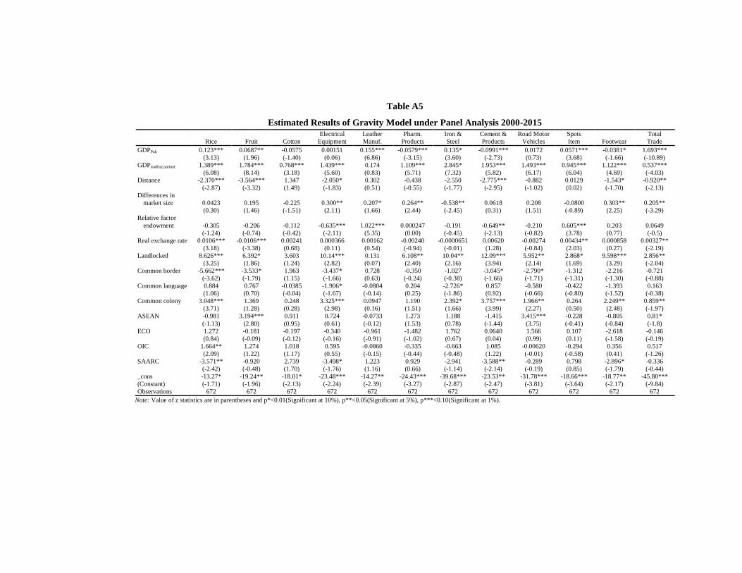
Table A5
Estimated Results of Gravity Model under Panel Analysis 2000-2015
Rice Fruit Cotton
Electrical
Equipment
Leather
Manuf.
Pharm.
Products
Iron &
Steel
Cement &
Products
Road Motor
Vehicles
Spots
Item Footwear
Total
Trade
GDPPak 0.123*** 0.0687** -0.0575 0.00151 0.155*** -0.0579*** 0.135* -0.0991*** 0.0172 0.0571*** -0.0381* 1.693***
(3.13) (1.96) (-1.40) (0.06) (6.86) (-3.15) (3.60) (-2.73) (0.73) (3.68) (-1.66) (-10.89)
GDPtrading partner 1.389*** 1.784*** 0.768*** 1.439*** 0.174 1.109*** 2.845* 1.953*** 1.493*** 0.945*** 1.122*** 0.537***
(6.08) (8.14) (3.18) (5.60) (0.83) (5.71) (7.32) (5.82) (6.17) (6.04) (4.69) (-4.03)
Distance -2.370*** -3.564*** 1.347 -2.050* 0.302 -0.438 -2.550 -2.775*** -0.882 0.0129 -1.543* -0.920**
(-2.87) (-3.32) (1.49) (-1.83) (0.51) (-0.55) (-1.77) (-2.95) (-1.02) (0.02) (-1.70) (-2.13)
Differences in
market size 0.0423 0.195 -0.225 0.300** 0.207* 0.264** -0.538** 0.0618 0.208 -0.0800 0.303** 0.205**
(0.30) (1.46) (-1.51) (2.11) (1.66) (2.44) (-2.45) (0.31) (1.51) (-0.89) (2.25) (-3.29)
Relative factor
endowment -0.305 -0.206 -0.112 -0.635*** 1.022*** 0.000247 -0.191 -0.649** -0.210 0.605*** 0.203 0.0649
(-1.24) (-0.74) (-0.42) (-2.11) (5.35) (0.00) (-0.45) (-2.13) (-0.82) (3.78) (0.77) (-0.5)
Real exchange rate 0.0106*** -0.0106*** 0.00241 0.000366 0.00162 -0.00240 -0.0000651 0.00620 -0.00274 0.00434** 0.000858 0.00327**
(3.18) (-3.38) (0.68) (0.11) (0.54) (-0.94) (-0.01) (1.28) (-0.84) (2.03) (0.27) (-2.19)
Landlocked 8.626*** 6.392* 3.603 10.14*** 0.131 6.108** 10.04** 12.09*** 5.952** 2.868* 9.598*** 2.856**
(3.25) (1.86) (1.24) (2.82) (0.07) (2.40) (2.16) (3.94) (2.14) (1.69) (3.29) (-2.04)
Common border -5.662*** -3.533* 1.963 -3.437* 0.728 -0.350 -1.027 -3.045* -2.790* -1.312 -2.216 -0.721
(-3.62) (-1.79) (1.15) (-1.66) (0.63) (-0.24) (-0.38) (-1.66) (-1.71) (-1.31) (-1.30) (-0.88)
Common language 0.884 0.767 -0.0385 -1.906* -0.0804 0.204 -2.726* 0.857 -0.580 -0.422 -1.393 0.163
(1.06) (0.70) (-0.04) (-1.67) (-0.14) (0.25) (-1.86) (0.92) (-0.66) (-0.80) (-1.52) (-0.38)
Common colony 3.048*** 1.369 0.248 3.325*** 0.0947 1.190 2.392* 3.757*** 1.966** 0.264 2.249** 0.859**
(3.71) (1.28) (0.28) (2.98) (0.16) (1.51) (1.66) (3.99) (2.27) (0.50) (2.48) (-1.97)
ASEAN -0.981 3.194*** 0.911 0.724 -0.0733 1.273 1.188 -1.415 3.415*** -0.228 -0.805 0.81*
(-1.13) (2.80) (0.95) (0.61) (-0.12) (1.53) (0.78) (-1.44) (3.75) (-0.41) (-0.84) (-1.8)
ECO 1.272 -0.181 -0.197 -0.340 -0.961 -1.482 1.762 0.0640
(0.04)
1.566 0.107 -2.618 -0.146
(0.84) (-0.09) (-0.12) (-0.16) (-0.91) (-1.02) (0.67) (0.99) (0.11) (-1.58) (-0.19)
OIC 1.664** 1.274 1.018 0.595 -0.0860 -0.335 -0.663 1.085 -0.00620 -0.294 0.356 0.517
(2.09) (1.22) (1.17) (0.55) (-0.15) (-0.44) (-0.48) (1.22) (-0.01) (-0.58) (0.41) (-1.26)
SAARC -3.571** -0.920 2.739 -3.498* 1.223 0.929 -2.941 -3.588** -0.289 0.798 -2.896* -0.336
(-2.42) (-0.48) (1.70) (-1.76) (1.16) (0.66) (-1.14) (-2.14) (-0.19) (0.85) (-1.79) (-0.44)
_cons -13.27* -19.24** -18.01* -23.48*** -14.27** -24.43*** -39.68*** -23.53** -31.78*** -18.66*** -18.77** -45.80***
(Constant) (-1.71) (-1.96) (-2.13) (-2.24) (-2.39) (-3.27) (-2.87) (-2.47) (-3.81) (-3.64) (-2.17) (-9.84)
Observations 672 672 672 672 672 672 672 672 672 672 672 672
Note: Value of z statistics are in parentheses and p*<0.01(Significant at 10%), p**<0.05(Significant at 5%), p***<0.10(Significant at 1%).

Table A6.0
Cross-Sectional Analysis with GLS (2001-2005)
Rice Cotton Fruits
Electrical
Equipment
Leather
Manuf.
Pharm.
Products
Iron &
Steel
Cement &
Products Footwear
Road motor
Vehicles
Sport
Items
Total
Trade
GDP ratio 0.708** -0.71** -0.191 -0.267 -0.0575 -0.0252 -1.099** -0.257 0.758** -0.399 -0.84*** 0.0085
(2.35) (-2.41) (-0.53) (-0.65) (-0.25) (-0.10) (-1.95) (-0.82) (2.14) (-1.24) (-5.56) (0.06)
Distance -0.127 0.295 -2.40*** -1.638* -0.228 -0.904 -1.476 -1.442* -0.888 -0.889 -0.312 -0.860**
(-0.17) (0.40) (-2.65) (-1.65) (-0.40) (-1.36) (-1.04) (-1.83) (-0.99) (-1.09) (-0.82) (-2.24)
Differences in
market size 0.344* 0.311* 0.500** 0.868*** 0.505*** 0.695*** 0.932*** 0.531*** 0.671*** 0.687*** 0.374*** 0.563***
(1.95) (1.82) (2.38) (3.63) (3.78) (4.49) (2.83) (2.90) (3.23) (3.64) (4.22) (6.32)
Relative factor
endowment 0.690** -0.58** 0.578* 0.246 0.614*** 0.231 0.131 0.0139 0.976*** -0.217 -0.0323 0.0172
(2.39) (-2.09) (1.68) (0.63) (2.81) (0.91) (0.24) (0.05) (2.87) (-0.70) (-0.22) (0.12)
Real exchange rate -0.006 0.011* -0.005 0.0142* 0.00705 0.00310 -0.0005 0.00925 0.00195 0.0113* 0.00680** 0.00425
(-0.91) (1.85) (-0.63) (1.71) (1.52) (0.58) (-0.05) (1.45) (0.27) (1.72) (2.21) (1.37)
Landlocked -7.091 11.55** 2.495 7.029 4.035 0.913 18.36* 10.53* -6.708 7.189 13.42*** 1.095
(-1.30) (2.18) (0.38) (0.95) (0.98) (0.19) (1.80) (1.86) (-1.05) (1.23) (4.89) (0.40)
Common border 0.383 -1.105 -0.931 -1.959 -0.795 -0.354 0.340 -0.615 0.629 -3.374** -3.03*** -0.810
(0.25) (-0.73) (-0.50) (-0.92) (-0.67) (-0.26) (0.12) (-0.38) (0.34) (-2.02) (-3.85) (-1.03)
Common language 1.730** -0.344 1.380 -2.101** -0.295 0.194 -1.842 1.628** -0.633 -0.683 -0.620* -0.0405
(2.34) (-0.48) (1.57) (-2.10) (-0.53) (0.30) (-1.34) (2.12) (-0.73) (-0.86) (-1.67) (-0.11)
Common colony 0.605 0.788 0.0380 2.518** 1.282** 0.357 2.321 1.842** 0.535 1.472* 1.359*** 0.698*
(0.72) (0.96) (0.04) (2.20) (2.01) (0.48) (1.48) (2.11) (0.54) (1.63) (3.21) (1.64)
ASEAN 0.331 0.361 4.641*** 2.412** -0.552 2.250*** 1.512 -0.286 1.124 3.349*** -1.57*** 1.037**
(0.39) (0.43) (4.55) (2.07) (-0.85) (2.99) (0.95) (-0.32) (1.11) (3.65) (-3.63) (2.39)
ECO -0.0776 0.735 -0.356 0.802 -0.914 -1.228 1.315 0.163 -2.405 2.542* -0.139 0.148
(-0.06) (0.58) (-0.23) (0.45) (-0.92) (-1.07) (0.54) (0.12) (-1.56) (1.81) (-0.21) (0.22)
OIC 2.149** 0.640 1.343* 0.656 -0.299 -1.233** -0.810 0.689 0.143 -0.731 -0.404 0.345
(3.11) (0.95) (1.63) (0.70) (-0.57) (-2.03) (-0.63) (0.96) (0.18) (-0.99) (-1.16) (0.99)
SAARC -0.724 -0.109 1.333 -1.939 -1.706 1.181 -2.311 -3.426** -1.347 -0.628 -1.963*** -1.042
(-0.51) (-0.08) (0.79) (-1.01) (-1.60) (0.95) (-0.88) (-2.34) (-0.81) (-0.42) (-2.77) (-1.46)
_cons -3.911 -1.725 9.722 -5.988 -7.816 -4.071 -8.197 1.023 -7.817 -3.561 1.453 2.202
(-0.56) (-0.26) (1.18) (-0.64) (-1.49) (-0.67) (-0.63) (0.14) (-0.96) (-0.48) (0.42) (0.63)
Observation 42 42 42 42 42 42 42 42 42 42 42 42
Note: Value of z statistics are in parentheses and p***<0.01(Significant at 1%), p**<0.05(Significant at 5%), p*<0.10(Significant at 10%).
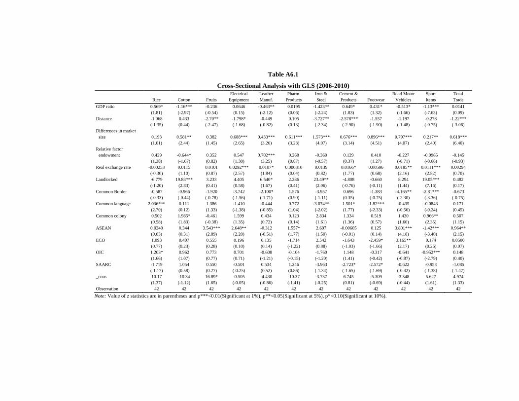
Table A6.1
Cross-Sectional Analysis with GLS (2006-2010)
Rice Cotton Fruits
Electrical
Equipment
Leather
Manuf.
Pharm.
Products
Iron &
Steel
Cement &
Products Footwear
Road Motor
Vehicles
Sport
Items
Total
Trade
GDP ratio 0.569* -1.16*** -0.236 0.0646 -0.463** 0.0195 -1.423** 0.649* 0.431* -0.513* -1.13*** 0.0141
(1.81) (-2.97) (-0.54) (0.15) (-2.12) (0.06) (-2.24) (1.83) (1.32) (-1.66) (-7.63) (0.09)
Distance -1.068 0.433 -2.70** -1.798* -0.449 0.105 -3.727** -2.578*** -1.557 -1.197 -0.278 -1.22***
(-1.35) (0.44) (-2.47) (-1.68) (-0.82) (0.13) (-2.34) (-2.90) (-1.90) (-1.48) (-0.75) (-3.06)
Differences in market
size 0.193 0.581** 0.382 0.688*** 0.433*** 0.611*** 1.573*** 0.676*** 0.896*** 0.797*** 0.217** 0.618***
(1.01) (2.44) (1.45) (2.65) (3.26) (3.23) (4.07) (3.14) (4.51) (4.07) (2.40) (6.40)
Relative factor
endowment 0.429 -0.644* 0.352 0.547 0.702*** 0.268 -0.360 0.129 0.410 -0.227 -0.0965 -0.145
(1.38) (-1.67) (0.82) (1.30) (3.25) (0.87) (-0.57) (0.37) (1.27) (-0.71) (-0.66) (-0.93)
Real exchange rate -0.00253 0.0115 0.0101 0.0292*** 0.0107* 0.000310 0.0139 0.0166* 0.00596 0.0185** 0.0111*** 0.00294
(-0.30) (1.10) (0.87) (2.57) (1.84) (0.04) (0.82) (1.77) (0.68) (2.16) (2.82) (0.70)
Landlocked -6.779 19.83*** 3.233 4.405 6.540* 2.286 23.49** -4.808 -0.660 8.294 19.05*** 0.482
(-1.20) (2.83) (0.41) (0.58) (1.67) (0.41) (2.06) (-0.76) (-0.11) (1.44) (7.16) (0.17)
Common Border -0.587 -0.966 -1.920 -3.742 -2.100* 1.576 -3.957 0.696 -1.383 -4.165** -2.81*** -0.673
(-0.33) (-0.44) (-0.78) (-1.56) (-1.71) (0.90) (-1.11) (0.35) (-0.75) (-2.30) (-3.36) (-0.75)
Common language 2.036*** 0.111 1.386 -1.410 -0.444 0.772 -3.074** 1.501* -1.82*** -0.435 -0.0843 0.171
(2.70) (0.12) (1.33) (-1.38) (-0.85) (1.04) (-2.02) (1.77) (-2.33) (-0.56) (-0.24) (0.45)
Common colony 0.502 1.985* -0.461 1.599 0.434 0.123 2.834 1.334 0.519 1.430 0.966** 0.507
(0.58) (1.83) (-0.38) (1.35) (0.72) (0.14) (1.61) (1.36) (0.57) (1.60) (2.35) (1.15)
ASEAN 0.0240 0.344 3.543*** 2.648** -0.312 1.557* 2.697 -0.00605 0.125 3.801*** -1.42*** 0.964**
(0.03) (0.31) (2.89) (2.20) (-0.51) (1.77) (1.50) (-0.01) (0.14) (4.18) (-3.40) (2.15)
ECO 1.093 0.407 0.555 0.196 0.135 -1.714 2.542 -1.643 -2.459* 3.165** 0.174 0.0500
(0.77) (0.23) (0.28) (0.10) (0.14) (-1.22) (0.88) (-1.03) (-1.66) (2.17) (0.26) (0.07)
OIC 1.203* 0.962 0.773 0.701 -0.608 -0.104 -1.760 1.148 -0.317 -0.641 -0.952*** 0.148
(1.66) (1.07) (0.77) (0.71) (-1.21) (-0.15) (-1.20) (1.41) (-0.42) (-0.87) (-2.79) (0.40)
SAARC -1.719 1.054 0.550 -0.501 0.534 1.246 -3.963 -2.723* -2.572* -0.622 -0.953 -1.085
(-1.17) (0.58) (0.27) (-0.25) (0.52) (0.86) (-1.34) (-1.65) (-1.69) (-0.42) (-1.38) (-1.47)
_cons 10.17 -10.34 16.89* -0.505 -4.430 -10.37 -3.737 6.745 -5.309 -3.348 5.627 4.974
(1.37) (-1.12) (1.65) (-0.05) (-0.86) (-1.41) (-0.25) (0.81) (-0.69) (-0.44) (1.61) (1.33)
Observation 42 42 42 42 42 42 42 42 42 42 42 42
Note: Value of z statistics are in parentheses and p***<0.01(Significant at 1%), p**<0.05(Significant at 5%), p*<0.10(Significant at 10%).

Table A6.2
Cross-Sectional Analysis with GLS (2011-2015)
Rice Cotton Fruits
Electrical
Equipment
Leather
Manuf.
Pharm.
Products
Iron &
Steel
Cement &
Products Footwear
Road Motor
Vehicles
Sport
Items
Total
Trade
GDP ratio 0.467 -1.29*** -0.419 0.220 -0.498** -0.0363 -1.17*** 0.210 -0.0566 -0.381 -1.069*** 0.108
(1.48) (-3.69) (-1.00) (0.53) (-2.49) (-0.11) (-3.09) (0.48) (-0.17) (-1.16) (-6.05) (0.62)
Distance -1.72** 0.552 -3.2*** -2.572*** -0.536 0.663 -4.43*** -1.404 -1.425* -1.506* -0.279 -1.38***
(-2.25) (0.65) (-3.19) (-2.57) (-1.11) (0.81) (-4.82) (-1.32) (-1.73) (-1.89) (-0.65) (-3.23)
Differences in market
size 0.587*** 0.633*** 0.463* 0.713*** 0.453*** 0.602*** 1.669*** 0.651** 0.796*** 1.006*** 0.248** 0.740***
(3.06) (2.99) (1.82) (2.85) (3.74) (2.95) (7.27) (2.44) (3.86) (5.04) (2.32) (6.93)
Relative factor
endowment 0.153 -0.776** 0.209 0.601 0.831*** 0.245 0.0920 -0.410 0.323 -0.210 0.0685 -0.117
(0.50) (-2.31) (0.52) (1.51) (4.32) (0.76) (0.25) (-0.97) (0.99) (-0.66) (0.40) (-0.69)
Real exchange rate 0.0125* 0.00691 0.0110 0.0326*** 0.0116** 0.00153 0.0111 0.0112 0.0130 0.0254*** 0.0144*** 0.00388
(1.65) (0.82) (1.09) (3.29) (2.40) (0.19) (1.22) (1.06) (1.59) (3.20) (3.40) (0.92)
Landlocked -3.560 24.28*** 7.168 1.326 5.007 4.434 20.27*** 0.131 6.347 9.067 16.34*** 0.375
(-0.64) (3.94) (0.96) (0.18) (1.42) (0.74) (3.03) (0.02) (1.06) (1.56) (5.23) (0.12)
Common Border -2.791 -1.093 -3.871 -5.664** -2.129 1.261 -3.203 -0.414 -2.514 -6.602*** -3.321*** -1.275
(-1.50) (-0.53) (-1.57) (-2.34) (-1.81) (0.64) (-1.44) (-0.16) (-1.26) (-3.41) (-3.20) (-1.23)
Common language 0.821 -0.489 1.766 -0.922 -0.169 0.398 -2.45*** 0.807 -1.597** -0.332 0.0911 -0.174
(1.08) (-0.58) (1.75) (-0.93) (-0.35) (0.49) (-2.70) (0.77) (-1.96) (-0.42) (0.21) (-0.41)
Common colony 0.988 2.202** -0.168 1.448 -0.0263 0.231 2.178** 1.817 0.908 1.433 0.998** 0.507
(1.15) (2.32) (-0.15) (1.29) (-0.05) (0.25) (2.11) (1.52) (0.98) (1.60) (2.07) (1.06)
ASEAN 0.162 0.309 2.856** 1.797 0.0716 1.520* 2.126** -0.775 -0.368 4.212*** -0.637 1.224**
(0.19) (0.33) (2.51) (1.61) (0.13) (1.67) (2.08) (-0.65) (-0.40) (4.73) (-1.33) (2.57)
ECO 1.118 -1.074 0.887 1.822 -0.0536 -1.045 1.481 1.838 -1.779 2.706* 1.036 -0.305
(0.77) (-0.67) (0.46) (0.96) (-0.06) (-0.68) (0.85) (0.91) (-1.14) (1.79) (1.28) (-0.38)
OIC 0.840 0.315 0.807 0.594 -0.412 -0.565 -1.125 -0.290 -0.233 -0.652 -1.204*** -0.376
(1.18) (0.40) (0.85) (0.64) (-0.91) (-0.74) (-1.31) (-0.29) (-0.30) (-0.88) (-3.01) (-0.95)
SAARC -2.599* 1.294 0.243 -0.00994 1.971** 2.003 -5.65*** 0.229 -1.888 -0.0450 0.207 -0.687
(-1.84) (0.83) (0.13) (-0.01) (2.21) (1.33) (-3.34) (0.12) (-1.24) (-0.03) (0.26) (-0.87)
_cons 6.420 -11.74 20.39** 4.929 -4.852 -14.39* -2.460 -0.685 -3.221 -6.880 4.141 3.128
(0.86) (-1.42) (2.05) (0.50) (-1.02) (-1.80) (-0.27) (-0.07) (-0.40) (-0.88) (0.99) (0.75)
Observation 42 42 42 42 42 42 42 42 42 42 42 42
Note: Value of z statistics are in parentheses and p***<0.01(Significant at 1%), p**<0.05(Significant at 5%), p*<0.10(Significant at 10%).

Table A7
Estimated Results of Gravity Model using Trade Cost Variable under Panel Analysis 2003-2012
Rice Fruit Cotton
Electrical
Equipment
Leather
Manuf.
Pharm.
Products Iron & Steel
Cement &
Products
Road Motor
Vehicles
Spots
Item Footwear Total Trade
GDPPak 0.273** 0.022 -0.0266 -0.0615 0.0139 -0.0983** -0.0194 0.00045 0.135* 0.0648 -0.029 0.0694
(-2.6) (-0.21) (-0.19) (-1.65) (-0.26) (-3.27) (-0.34) (-0.01) (-2.26) (-1.5) (-1.01) -0.16
GDPtrading partner 4.653** 2.335 5.412* -0.739 1.373 -2.795** 3.148 2.654 0.629 1.043 0.576 2.821***
(-2.61) (-1.29) (-2.32) (-0.57) (-0.73) (-2.69) (-1.58) (-1.12) (-0.3) (-0.7) (-0.58) (-4.71)
Trade cost -
0.0653***
-
0.0508***
-
0.0794*** -0.0339** 0.0436** 0.00438 0.00625 -0.0189 0.00818
-
0.0976*** -0.0028 -0.0514***
(-6.08) (-4.65) (-5.64) (-3.06) (-2.71) (-0.49) (-0.36) (-0.92) (-0.46) (-7.59) (-0.33) (-9.23)
Differences in market size -5.680** -1.945 -5.899** -0.896 -2.425 1.86 -2.951 -1.399 -3.463 -0.496 -1.81 -1.907**
(-3.28) (-1.11) (-2.60) (-0.69) (-1.29) (-1.77) (-1.47) (-0.58) (-1.65) (-0.33) (-1.81) (-3.23)
Relative factor
endowment 4.523*** 1.121 3.261*** -1.802*** 0.138 0.659 1.532 2.012* 1.145 -0.866 1.080** 1.186***
(-6.56) (-1.6) (-3.6) (-3.48) (-0.18) (-1.58) (-1.91) (-2.1) (-1.37) (-1.44) (-2.71) (-5.03)
Real exchange rate 0.00559 0.0138** -0.0061 0.0178*** 0.0123** 0.00723** -0.0041 0.00172 0.0158*** 0.00309 0.0133*** -0.002
(-1.34) (-3.25) (-1.11) (-6.48) (-3.09) (-3.26) (-0.96) (-0.34) (-3.56) (-0.97) (-6.29) (-1.51)
Common border 8.882*** 2.061 10.16*** -4.629*** -1.445 1.387 6.781*** 8.208*** 3.097* -5.053*** 0.543 2.544***
(-5.83) (-1.33) (-5.08) (-5.02) (-1.08) (-1.86) (-4.75) (-4.82) (-2.08) (-4.72) (-0.77) (-6.1)
Common language 0.318 0.24 1.858*** -0.166 1.108** 0.11 -1.233** 1.153* 0.651 -3.055*** -0.251 -0.973***
(-0.74) (-0.55) (-3.3) (-0.61) (-2.81) (-0.5) (-2.94) (-2.3) (-1.49) (-9.69) (-1.20) (-7.92)
Common colony -9.954*** -2.189 -10.02*** -0.253 0.406 1.072 -0.268 -0.544 -3.778 1.114 -0.891 -2.086***
(-6.07) (-1.31) (-4.65) (-0.21) -0.23 -1.08 (-0.14) (-0.24) (-1.91) (-0.78) (-0.94) (-3.74)
ASEAN 6.022*** 2.141 4.885** -4.551*** -5.705*** 0.927 0.936 -1.163 -4.573* 2.248 -0.994 1.893***
(-4.2) (-1.47) (-2.59) (-3.93) (-3.40) (-0.99) (-0.52) (-0.54) (-2.45) -1.67 (-1.12) (-3.59)
OIC 1.978 -1.303 2.518 -4.205*** -2.075 -3.328*** -1.395 5.782*** -3.489* -8.097*** -4.081*** -0.214
(-1.78) (-1.15) (-1.72) (-4.86) (-1.65) (-4.77) (-1.04) -3.62 (-2.50) (-8.06) (-6.13) (-0.54)
SAARC 12.86*** 7.852** 10.15** -7.807*** -5.155 -1.139 -0.762 3.495 -3.41 -0.579 -0.236 5.463***
(-4.96) (-2.97) (-2.98) (-3.90) (-1.77) (-0.71) (-0.25) -0.95 (-1.06) (-0.25) (-0.15) (-6.01)
_cons 28.24** 24.57* 2.026 67.35*** 28.76** 36.06*** -4.26 36.18** 86.52*** 13.75 42.12*** -11.688
(Constant) (-2.44) -1.62 -0.17 -7.19 -2.11 -4.77 (-0.29) (-2.09) -5.73 -1.26 -5.84 (-1.17)
Observations 100 100 100 100 100 100 100 100 100 100 100 100
Note: Value of z statistics are in parentheses and p*<0.01(Significant at 10%), p**<0.05(Significant at 5%), p***<0.10(Significant at 1%).
Economic & Cultural Distance & Regional Integration 269
REFERENCES
Abbas, S., & Waheed, A. (2015). Pakistan’s potential export flow: The gravity model
approach. The Journal of Developing Areas, 49(4), 367-378.
Achakzai, J. K. (2006). Intra-ECO trade: A potential region for Pakistan’s future
trade. The Pakistan Development Review, 425–437.
Akhter, N., & Ghani, E. (2010). Regional integration in South Asia: An analysis of trade
flows using the gravity model. The Pakistan Development Review, 105–118.
Akram, A. (2013). Pak-SAARC intra-industry trade (No. 2013: 93). Pakistan Institute of
Development Economics, Islamabad.
Alleyne, A., & Lorde, T. (2014). A gravity model approach to analysing the trade
performance of CARICOM member states. Applied Econometrics and International
Development, 14(2).
Altaf, S., Mahmood, Z., & Noureen, S. (n. d.) Trade costs of Pakistan with its major
trading partners: Measurement and its determinants. Perspectives on Pakistan’s Trade
and Development, 175.
Anderson, J. E. (1979). A theoretical foundation for the gravity equation. The American
Economic Review, 69(1), 106–116.
Anderson, J. E., & Van Wincoop, E. (2003). Gravity with Gravitas: A solution to the
border puzzle. The American Economic Review, 93(1), 170–192.
Anderton, R., & Skudelny, F. (2001). Exchange rate volatility and Euro area imports.
Bacchetta, P., & Van Wincoop, E. (2000). Does exchange-rate stability increase trade and
welfare? American Economic Review, 1093–1109.
Bahmani-Oskooee, Iqbal J. & Nosheen, M. (2016). Commodity trade between Pakistan
and the US: Is there evidence of the J-curve?. Applied Economics, 48 (11), 957–965.
Bahmani-Oskooee, M. (1986). Determinants of international trade flows: Case of
developing countries. Journal of Development Economics 20:107–123.
Bahmani-Oskooee, Iqbal, J. & Khan, S. H. (2016). Impact of exchange rate volatility on
the commodity trade between Pakistan and the US, Economic Change and
Restructuring, 2017, 50(2),16.
Baldwin, R. E. (1994). Towards an integrated Europe (Vol. 25, No. 234). London:
Centre for Economic Policy Research.
Baltagi, B. H., Egger, P., & Pfaffermayr, M. (2003). A Generalised Design for Bilateral
Trade Flow Models. Economics Letters, 80(3), 391–397.
Bergstrand, J. H. (1985). The gravity equation in international trade: Some
microeconomic foundations and empirical evidence. The Review of Economics and
Statistics, 474–481.
Bergstrand, J. H. (1989). The generalised gravity equation, monopolistic competition, and
the factor-proportions theory in international trade. The Review of Economics and
Statistics, 143–153.
Bikker, J. A. (1987). An international trade flow model with substitution: An extension of
the gravity model. Kyklos, 40(3), 315–337.
Boisso, D., & Ferrantino, M. (1997). Economic distance, cultural distance, and openness in
international trade: Empirical puzzles. Journal of Economic Integration, 456–484.
Boughanmi, H. (2008). The trade potential of the Arab Gulf cooperation countries
(GCC): A gravity model approach. Journal of Economic Integration, 42–56.
270 Salahuddin, Iqbal, and Nosheen
Buongiorno, J. (2015). Monetary union and forest products trade—The case of the euro.
Journal for Economics, 21, 238–24.
Buongiorno, J. (2016). Gravity model of forest products trade: Application to forecasting
and policy analysis. Forestry, 89, 117–126.
Butt, W. A. (2008). Pakistan’s export potential: A gravity model analysis (No. 23).
Research Department, State Bank of Pakistan.
Carrillo-Tudela, C., & Li, C. A. (2004). Trade blocs and the gravity model: Evidence
from Latin American countries. Journal of Economic Integration, 667–689.
Castillo, J. S., Villanueva, E. C., & García‐Cortijo, M. C. (2016). The international wine
trade and its new export dynamics (1988–2012): A gravity model
approach. Agribusiness, 32(4), 466–481.
Christie, E. (2002). Potential trade in Southeast Europe: A gravity model approach (Vol.
21). Verein “Wiener Institut für Internationale Wirtschaftsvergleiche”.
Danial, P. (1990). Exchange rate risk and U.S. agriculture trade flows. American Journal
of Agriculture Economics, 72(3), 94–700.
De Grauwe, P., & Skudelny, F. (2000). The impact of EMU on trade
flows. Weltwirtschaftliches Archiv, 136(3), 381–402.
De, P. (2006). Trade, infrastructure and transaction costs: The imperatives for Asian
economic cooperation. Journal of Economic Integration, 708–735.
Egger, P. (2002). An econometric view on the estimation of gravity models and the
calculation of trade potentials. The World Economy, 25(2), 297–312.
Egger, P., & Pfaffermayr, M. (2003). The proper panel econometric specification of the
gravity equation: A three-way model with bilateral interaction effects. Empirical
Economics, 28(3), 571–580.
Eichengreen, B., & Irwin, D. A. (1998). The role of history in bilateral trade flows.
In The regionalisation of the world economy (pp. 33-62). University of Chicago Press.
Ekanayake, E. M., Mukherjee, A., & Veeramacheneni, B. (2010). Trade blocs and the
gravity model: A study of economic integration among Asian developing
countries. Journal of Economic Integration. 627–643.
Feenstra, R. C. (1998). Integration of trade and disintegration of production in the global
economy. Journal of Economic Perspectives, 12(4), 31–50.
Frankel, J. A., Stein, E., & Wei, S. J. (1997). Regional trading blocs in the world
economic system. Peterson Institute.
Frankel, J., Stein, E., & Wei, S. J. (1995). Trading blocs and the Americas: The natural, the
unnatural, and the super-natural. Journal of Development Economics, 47(1), 61–95.
Gould, D. M. (1998). Has NAFTA changed North American trade? Economic Review-
Federal Reserve Bank of Dallas, 12.
Gul, N. and Yasin, Hafiz M. (2011). The trade potential of Pakistan: An application of
the gravity model. Lahore Journal of Economics, 16(1), 23–62.
Hamilton, C. B., & Winters, L. A. (1992). Opening up international trade with Eastern
Europe. Economic Policy, 7(14), 77–116.
Harrigan, J. (1994). Scale economies and the volume of trade. The Review of Economics
and Statistics, 321–328.
Harris, M. N., & Mátyás, L. (1998). The econometrics of gravity models. Melbourne
Institute of Applied Economic and Social Research.
Economic & Cultural Distance & Regional Integration 271
Hassan, M. K. (2000). Trade relations with SAARC countries and trade policies of
Bangladesh. Journal of Economic Cooperation, 21(3), 99–151.
Hassan, M. K. (2001). Is SAARC a viable economic bloc? Evidence from gravity
model. Journal of Asian Economics, 12(2), 263–290.
Helpman, E., & Krugman, P. R. (1985). Market structure and foreign trade: Increasing
returns, imperfect competition, and the international economy. MIT Press.
Hussain, M. (2017). Globalisation and gravity model of trade of Pakistan: A PPML-
estimator analysis. Management and Administrative Science Review, 6(1), 15–27.
Hutchinson, W. K. (2005). “Linguistic distance” as a determinant of bilateral
trade. Southern Economic Journal, 1–15.
Insel, A., & Tekce, M. (2009). Bilateral trade flows of the Gulf cooperation council
countries: A new approach to gravity model. Topics in Middle Eastern and North
African Economies. 11.
Iqbal, J. (2016). An analysis of Pakistan’s exports using gravity model. Abasyn J Soc
Sci, 9(1), 271.
Irshad, M. S., Xin, Q., Hui, Z. & Arshad, H. (2018). An empirical analysis of Pakistan’s
bilateral trade and trade potential with China: A gravity model approach. Cogent
Economics & Finance, 6(1), 1–18.
Irshad, M. S., Xin, Q., Hui, Z., & Arshad, H. (2018). An empirical analysis of Pakistan’s
bilateral trade and trade potential with China: A gravity model approach. Cogent
Economics & Finance, 6(1), 1–18.
Irshad, M. S., Xin, Q., Shahriar, S., & Arshad, H. (2018). A panel data analysis of Chinas
trade pattern with OPEC members: Gravity model approach. Asian Economic and
Financial Review, 8(1), 103–116.
Irshad, M. S., Xin, Q., Shahriar, S., & Arshad, H. (2018). A panel data analysis of
China’s trade pattern with OPEC members: Gravity model approach. Asian Economic
and Financial Review, 8(1), 103–116.
Jafari, Y., Ismail, M. A., & Kouhestani, M. S. (2011). Determinants of trade flows among
D8 countries: Evidence from the gravity model. Journal of Economic Cooperation &
Development, 32(3).
Jakab, Z. M., Kovács, M. A., & Oszlay, A. (2001). How far has trade integration
advanced?: An analysis of the actual and potential trade of three Central and Eastern
European countries. Journal of Comparative Economics, 29(2), 276–292.
Jayasinghe, S., & Sarker, R. (2008). Effects of regional trade agreements on trade in
agrifood products: Evidence from gravity modeling using disaggregated data. Review
of Agricultural Economics, 61–81.
Kabir, M., & Salim, R. (2010). Can gravity model explain BIMSTEC’s trade? Journal of
Economic Integration, 143–165.
Karemera, D., Koo, W., Smalls, G., & Whiteside, L. (2015). Trade creation and diversion
effects and exchange rate volatility in the global meat trade. Journal of Economic
Integration, 240–268.
Karemera, D., Managi, S., Reuben, L., & Spann, O. (2011). The impacts of exchange rate
volatility on vegetable trade flows. Applied Economics, 43(13), 1607–1616.
Karemera, D., Reinstra-Munnicha, P., & Onyeocha, J. (2009). Impacts of free trade
agreement on US State vegetable and fruit trade flows. Journal of Economic
Integration, 116–134.

272 Salahuddin, Iqbal, and Nosheen
Karemera, D., Smith, W. I., Ojah, K., & Cole, J. A. (1999). A gravity model analysis of
the benefits of economic integration in the Pacific Rim. Journal of Economic
Integration, 347–367.
Khan, H. I., & Mahmood, Z. (n.d.). Trade creation vs. trade diversion and general
equilibrium effects in regional and bilateral free trade agreements of
Pakistan. Perspectives on Pakistan’s Trade and Development, 39.
Khan, S., & Khan, D. (2013). An empirical analysis of Pakistan’s bilateral trade: A
gravity model approach. Romanian Economic Journal, 16(48).
Kien, N. T. (2009). Gravity model by panel data approach: An empirical application with
implications for the ASEAN free trade area. ASEAN Economic Bulletin, 26(3), 266–
277.
Koo, W. W., Karemera, D., & Taylor, R. (1994). A gravity model analysis of meat trade
policies. Agricultural Economics, 10(1), 81–88.
Krueger, A. O. (1999). Are preferential trading arrangements trade-liberalising or
protectionist? The Journal of Economic Perspectives, 13(4), 105–124.
Krueger, A. O. (1999). Trade creation and trade diversion under NAFTA (No. w7429).
National Bureau of Economic Research.
Kumar, Chaudhary, Li, Xiumin, and Khan, Muhammad Kamran (2018). The factors
affecting Nepal’s trade: Gravity model analysis, European Academic Research V(12),
6766–6782.
Lee, J. W., & Swagel, P. (1997). Trade barriers and trade flows across countries and
industries. Review of Economics and Statistics, 79(3), 372–382.
Linnemann, H. (1966). An econometric study of international trade flows (Vol. 234).
Amsterdam: North-Holland Publishing Company.
Lundmark, R. (2018). Analysis and projection of global iron ore trade: A panel data
gravity model approach, Mineral Economics, 31(1), 191–202.
Malik, S., & Chaudhary, A. R. (2011). A static analysis of Pakistan’s trade policy with
selected Asian countries. Theoretical and Applied Economics, 12(12), 71
Martínez-Zarzoso, I., & Nowak-Lehmann, F. (2003). Augmented gravity model: An
empirical application to Mercosur-European union trade flows. Journal of Applied
Economics, 6(2), 291–316.
Mathur, S. K. (2000). Pattern of international trade, new trade theories and evidence from
gravity equation analysis. Indian Economic Journal, 47(4), 68.
McCallum, J. (1995). National borders matter: Canada-US regional trade patterns. The
American Economic Review, 85(3), 615–623.
Narayan, S. & Nguyen, T. T. (2016). Does the trade gravity model depend on trading
partners? Some evidence from Vietnam and her 54 trading partners. International
Review of Economics &Finance, 41, 220–237.
Oguledo, V., & MacPhee, C. R. (1994). Gravity models: A reformulation and an
application to discriminatory trade arrangements. Applied Economics, 26(2), 107–120.
Olofsson C., Wadsten, J., and Lundmark, R. (2017) Renewable energy trade in Europe:
efficient use of biofuels. 15th International Association of Energy Economics
European Conference, 3–6 September, 2017, Vienna, Austria
Paas, T. (2000). Gravity approach for modelling trade flows between Estonia and the
main trading partners.

Economic & Cultural Distance & Regional Integration 273
Peterson E, Grant J, Roberts D, Karov V (2013). Evaluating the trade restrictiveness of
phytosanitary measures on U.S. fresh fruit and vegetable imports. Am. J. Agric. Econ.,
95, 842–858.
Rahapakse, P., & Arunatilake, N. (1997). Would a reduction in trade barriers promote
intra-SAARC trade?: A Sri Lankan perspective. Journal of Asian Economics, 8(1),
95–115.
Rahman, M., (2003). A panel data analysis of Bangladesh’s trade: The gravity model
approach. BIISS Journal, 19(1).
Reichman, J. H., & Samuelson, P. (1997). Intellectual property rights in data. Vand. L.
Rev., 50, 49.
Salim, S., & Mahmood, Z. (2015). Factors shaping exports of cultural goods from
Pakistan. NUST Journal of Social Sciences and Humanities, 73–86.
Sharma, S. C., & Chua, S. Y. (2000). ASEAN: Economic integration and intra-regional
trade. Applied Economics Letters 7(3), 165–169.
Soloaga, I., & Wintersb, L. A. (2001). Regionalism in the nineties: What effect on
trade? The North American Journal of Economics and Finance, 12(1), 1–29.
Tinbergen, J. (1962). Shaping the world economy; Suggestions for an international
economic policy. Books (Jan Tinbergen).
Zaheer, R., Nizami, U., & Niazi, M. F. K. (2013). 31 Years Intra-Industry Trade of
Pakistan. European Journal of Business and Management, 5(31).
Zahniser, S. S., Pick, D., Pompelli, G., & Gehlhar, M. J. (2002). Regionalism in the
western hemisphere and its impact on U.S. agricultural exports: A gravity model
analysis. Am. J. Agric. Econ., 84, 791–797.
Zhang, J., & Kristensen, G. (1995). A gravity model with variable coefficients: The EEC
trade with third countries. Geographical Analysis, 27(4), 307–320.