econ/fin 250: forecasting in finance and economics...
TRANSCRIPT
ECON/FIN 250: Forecasting in Finance and Economics:Section 3.2 Filtering Time Series
Patrick Herb
Brandeis University
Spring 2016
Patrick Herb (Brandeis University) Filtering Time Series ECON/FIN 250: Spring 2016 1 / 39

Course Overview
1 General Filtering Thoughts
2 Two-Sided Filters
3 One-Sided Filters
4 Local Trends
Patrick Herb (Brandeis University) Filtering Time Series ECON/FIN 250: Spring 2016 2 / 39

General Filtering Thoughts
Time series tools that can:Estimate TrendsSmooth Out NoiseAdjust for SeasonalityMake ForecastsSeparate the Cycle from the Trend
Somewhat ad hocCommon, simple rules used in business forecastingRelated to technical analysis in finance
Patrick Herb (Brandeis University) Filtering Time Series ECON/FIN 250: Spring 2016 3 / 39

Two-Sided Filters
1 General Filtering Thoughts
2 Two-Sided Filters
3 One-Sided Filters
4 Local Trends
Patrick Herb (Brandeis University) Filtering Time Series ECON/FIN 250: Spring 2016 4 / 39

Moving Average Filter
Uses Data Before & After time = tSmooths Data Using Future & Past InformationCan Choose Information SetCan Weight Observations EquallyCan Choose Alternative WeightsNot Useful for ForecastingCan Improve Understanding of the Data
Patrick Herb (Brandeis University) Filtering Time Series ECON/FIN 250: Spring 2016 5 / 39

Moving Average Filter
Equally Weighted
y∗t = 1
2m + 1
m∑j=−m
yt+j (1)
Alternative Weighting
y∗t =
m∑j=−m
ωjyt+j (2)
Weights should have the property:m∑
j=−mωj = 1 (3)
Patrick Herb (Brandeis University) Filtering Time Series ECON/FIN 250: Spring 2016 6 / 39
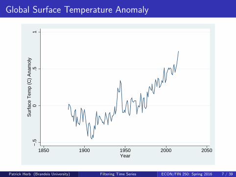
Global Surface Temperature Anomaly
−.5
0.5
1S
urfa
ce T
emp
(C)
Ana
mol
y
1850 1900 1950 2000 2050Year
Patrick Herb (Brandeis University) Filtering Time Series ECON/FIN 250: Spring 2016 7 / 39

Global Surface Temperature Anomaly
Let’s use an equally weighted moving average filter to reduce some of thenoise. Try m = 2use temperaturetsset yeartssmooth ma tempma = tempa , window (2 1 2)tsline tempa tempma
Patrick Herb (Brandeis University) Filtering Time Series ECON/FIN 250: Spring 2016 8 / 39

Global Surface Temperature Anomaly
−.5
0.5
1
1850 1900 1950 2000 2050Year
Surface Temp (C) Anamoly ma: x(t)= tempa: window(2 1 2)
Patrick Herb (Brandeis University) Filtering Time Series ECON/FIN 250: Spring 2016 9 / 39

Global Surface Temperature Anomaly
Still pretty noisy. Try m = 5tssmooth ma temp_ma = tempa , window (5 1 5)tsline tempa temp_ma
Patrick Herb (Brandeis University) Filtering Time Series ECON/FIN 250: Spring 2016 10 / 39

Global Surface Temperature Anomaly
−.5
0.5
1
1850 1900 1950 2000 2050Year
Surface Temp (C) Anamoly ma: x(t)= tempa: window(5 1 5)
Patrick Herb (Brandeis University) Filtering Time Series ECON/FIN 250: Spring 2016 11 / 39
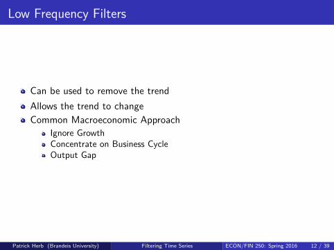
Low Frequency Filters
Can be used to remove the trendAllows the trend to changeCommon Macroeconomic Approach
Ignore GrowthConcentrate on Business CycleOutput Gap
Patrick Herb (Brandeis University) Filtering Time Series ECON/FIN 250: Spring 2016 12 / 39

Low Frequency Filters
ExamplesHodrick / Prescott FilterBaxter / KingButterworth
Type: help filter
Patrick Herb (Brandeis University) Filtering Time Series ECON/FIN 250: Spring 2016 13 / 39

Hodrick / Prescott Filter
The HP Filter:
miny∗
t
T∑t=1
(yt − y∗t )2 + λ
T−1∑t=2
[(y∗t+1 − y∗
t )− (y∗t − y∗
t−1]2 (4)
This filter is approximately a two-way moving average with weights subjectto a damped harmonic
λ is a positive smoothing parameterSmaller λ, penalizes variability in the cyclical componentLarger λ, penalizes variability in the growth component
Patrick Herb (Brandeis University) Filtering Time Series ECON/FIN 250: Spring 2016 14 / 39
Hodrick / Prescott Filter
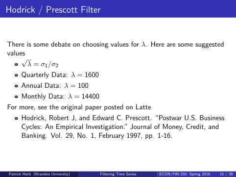
There is some debate on choosing values for λ. Here are some suggestedvalues√
λ = σ1/σ2
Quarterly Data: λ = 1600Annual Data: λ = 100Monthly Data: λ = 14400
For more, see the original paper posted on LatteHodrick, Robert J, and Edward C. Prescott. “Postwar U.S. BusinessCycles: An Empirical Investigation.” Journal of Money, Credit, andBanking. Vol. 29, No. 1, February 1997, pp. 1-16.
Patrick Herb (Brandeis University) Filtering Time Series ECON/FIN 250: Spring 2016 15 / 39
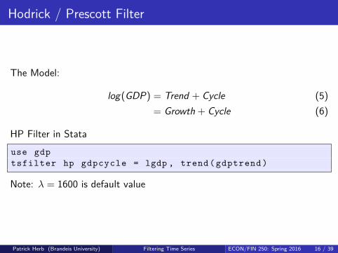
Hodrick / Prescott Filter
The Model:
log(GDP) = Trend + Cycle (5)= Growth + Cycle (6)
HP Filter in Statause gdptsfilter hp gdpcycle = lgdp , trend( gdptrend )
Note: λ = 1600 is default value
Patrick Herb (Brandeis University) Filtering Time Series ECON/FIN 250: Spring 2016 16 / 39

Log GDP & HP Trend
7.5
88.
59
9.5
1947q3 1964q3 1981q3 1998q3 2015q3dateq
lgdp lgdp trend component from hp filter
Patrick Herb (Brandeis University) Filtering Time Series ECON/FIN 250: Spring 2016 17 / 39

Log GDP & HP Trend
9.4
9.5
9.6
9.7
2000q1 2005q1 2010q1 2015q1dateq
lgdp lgdp trend component from hp filter
tsline lgdp gdptrend if dateq > tq (2000q1)
Patrick Herb (Brandeis University) Filtering Time Series ECON/FIN 250: Spring 2016 18 / 39
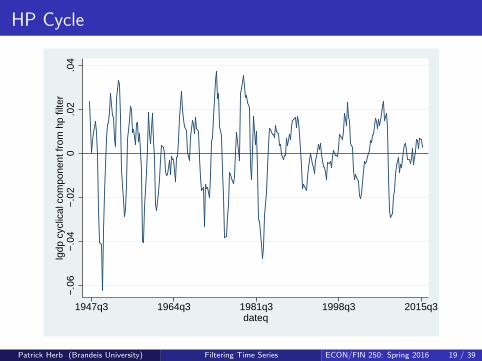
HP Cycle
−.0
6−
.04
−.0
20
.02
.04
lgdp
cyc
lical
com
pone
nt fr
om h
p fil
ter
1947q3 1964q3 1981q3 1998q3 2015q3dateq
Patrick Herb (Brandeis University) Filtering Time Series ECON/FIN 250: Spring 2016 19 / 39

Business Cycles & HP Filter
Much of modern macroeconomics applies the HP filter to many series toseparate the trend from the cycle:
GDPConsumptionInvestment
Then looks at the comovement between the cyclical components
Patrick Herb (Brandeis University) Filtering Time Series ECON/FIN 250: Spring 2016 20 / 39
One-Sided Filters
1 General Filtering Thoughts
2 Two-Sided Filters
3 One-Sided Filters
4 Local Trends
Patrick Herb (Brandeis University) Filtering Time Series ECON/FIN 250: Spring 2016 21 / 39
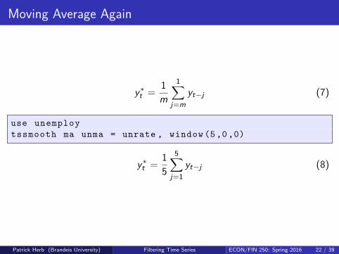
Moving Average Again
y∗t = 1
m
1∑j=m
yt−j (7)
use unemploytssmooth ma unma = unrate , window (5 ,0 ,0)
y∗t = 1
5
5∑j=1
yt−j (8)
Patrick Herb (Brandeis University) Filtering Time Series ECON/FIN 250: Spring 2016 22 / 39

Exponential Weighted Moving Average (EWMA)
Average of past valuesDecreasing (exponentially) weightsRelated to many ideas / models in economics
Adaptive Expectations (Friedman)Rational ExpectationsAutoregressive ModelsRiskmetricsGARCH Models
Patrick Herb (Brandeis University) Filtering Time Series ECON/FIN 250: Spring 2016 23 / 39
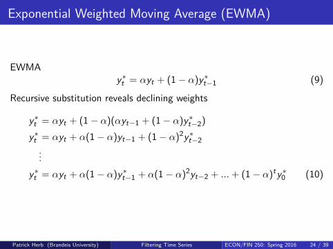
Exponential Weighted Moving Average (EWMA)
EWMAy∗
t = αyt + (1− α)y∗t−1 (9)
Recursive substitution reveals declining weights
y∗t = αyt + (1− α)(αyt−1 + (1− α)y∗
t−2)y∗
t = αyt + α(1− α)yt−1 + (1− α)2y∗t−2
...y∗
t = αyt + α(1− α)y∗t−1 + α(1− α)2yt−2 + ...+ (1− α)ty∗
0 (10)
Patrick Herb (Brandeis University) Filtering Time Series ECON/FIN 250: Spring 2016 24 / 39

Exponential Weighted Moving Average (EWMA)
2 4 6 8 10 12 14 16 18 20
yt-j
0.05
0.1
0.15
0.2
0.25
0.3W
eigh
t
α = 0.3α = 0.2α = 0.1
Patrick Herb (Brandeis University) Filtering Time Series ECON/FIN 250: Spring 2016 25 / 39
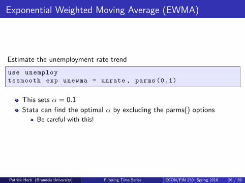
Exponential Weighted Moving Average (EWMA)
Estimate the unemployment rate trenduse unemploytssmooth exp unewma = unrate , parms (0.1)
This sets α = 0.1Stata can find the optimal α by excluding the parms() options
Be careful with this!
Patrick Herb (Brandeis University) Filtering Time Series ECON/FIN 250: Spring 2016 26 / 39

Exponential Weighted Moving Average (EWMA)
24
68
10
1950m1 1960m1 1970m1 1980m1 1990m1 2000m1 2010m1 2020m1datem
unrate exp parms(0.1000) = unrate
Patrick Herb (Brandeis University) Filtering Time Series ECON/FIN 250: Spring 2016 27 / 39

The Optimality of the EWMA
Suppose your time series comes from the following process:
xt = xt−1 + et xt = random walkyt = xt + ηt et , ηt = white noise
You do not observe xt
This implies yt is a random walk plus noiseIn this case, EWMA is the optimal forecast
Patrick Herb (Brandeis University) Filtering Time Series ECON/FIN 250: Spring 2016 28 / 39
Local Trends
1 General Filtering Thoughts
2 Two-Sided Filters
3 One-Sided Filters
4 Local Trends
Patrick Herb (Brandeis University) Filtering Time Series ECON/FIN 250: Spring 2016 29 / 39

Double Exponential Weighted Moving Average (DEWMA)
Filter Oncey∗
t = αyt + (1− α)y∗t−1 (11)
Filter Againy∗∗
t = αy∗t + (1− α)y∗∗
t−1 (12)
The double filter can follow local trendsThe trend can keep going up when the observed yt is going downGetting initial values for y∗
0 , y∗∗0 can be tricky
Patrick Herb (Brandeis University) Filtering Time Series ECON/FIN 250: Spring 2016 30 / 39

Double Exponential Weighted Moving Average
Estimate the unemployment rate trend using the double exponentialweighted moving averageuse unemploytssmooth dexp unema = unrate , parms (0.1)tsline unrate unema
Patrick Herb (Brandeis University) Filtering Time Series ECON/FIN 250: Spring 2016 31 / 39

Double Exponential Weighted Moving Average
24
68
10
1950m1 1960m1 1970m1 1980m1 1990m1 2000m1 2010m1 2020m1datem
unrate dexp parms(0.1000) = unrate
Patrick Herb (Brandeis University) Filtering Time Series ECON/FIN 250: Spring 2016 32 / 39
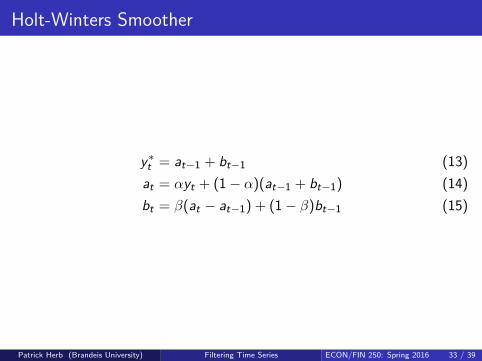
Holt-Winters Smoother
y∗t = at−1 + bt−1 (13)
at = αyt + (1− α)(at−1 + bt−1) (14)bt = β(at − at−1) + (1− β)bt−1 (15)
Patrick Herb (Brandeis University) Filtering Time Series ECON/FIN 250: Spring 2016 33 / 39
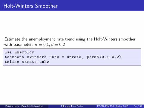
Holt-Winters Smoother
Estimate the unemployment rate trend using the Holt-Winters smootherwith parameters α = 0.1, β = 0.2use unemploytssmooth hwinters unhw = unrate , parms (0.1 0.2)tsline unrate unhw
Patrick Herb (Brandeis University) Filtering Time Series ECON/FIN 250: Spring 2016 34 / 39

Holt-Winters & Unemployment Rate
24
68
1012
1950m1 1960m1 1970m1 1980m1 1990m1 2000m1 2010m1 2020m1datem
unrate hw parms(0.100 0.200) = unrate
Patrick Herb (Brandeis University) Filtering Time Series ECON/FIN 250: Spring 2016 35 / 39

Holt-Winters Seasonal Smoother
Seasonal version of Holt-WintersSt is a repeating seasonal adjustmentThis is the multiplicative version (there is an additive version)s specifies the period of the seasonality
monthly data would have s = 12
y∗t = (at−1 + bt−1)St (16)
at = αyt
St−s) + (1− α)(at−1 + bt−1) (17)
bt = β(at − at−1) + (1− β)bt−1 (18)
St = γytat
+ (1− γ)St−s (19)
Patrick Herb (Brandeis University) Filtering Time Series ECON/FIN 250: Spring 2016 36 / 39
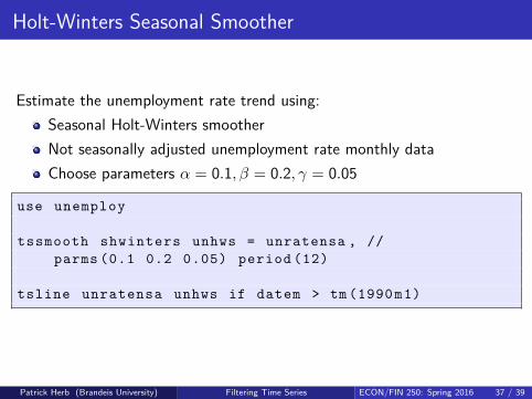
Holt-Winters Seasonal Smoother
Estimate the unemployment rate trend using:Seasonal Holt-Winters smootherNot seasonally adjusted unemployment rate monthly dataChoose parameters α = 0.1, β = 0.2, γ = 0.05
use unemploy
tssmooth shwinters unhws = unratensa , //parms (0.1 0.2 0.05) period (12)
tsline unratensa unhws if datem > tm (1990m1)
Patrick Herb (Brandeis University) Filtering Time Series ECON/FIN 250: Spring 2016 37 / 39

Seasonal Holt-Winters & Unemployment Rate NSA
46
810
12
1995m1 2000m1 2005m1 2010m1 2015m1datem
unratensa shw parms(0.100 0.200 0.050) = unratensa
Patrick Herb (Brandeis University) Filtering Time Series ECON/FIN 250: Spring 2016 38 / 39

Summary
yt = (Trend) + (Seasonal) + (Cycle) + (Noise) (20)
Filters can help separate partsFilters can help smooth out the noiseNot necessarily predictiveSometimes difficult to estimate
Initial value problemsAlso, a little ad hoc
Not clear what the data generating process is
Patrick Herb (Brandeis University) Filtering Time Series ECON/FIN 250: Spring 2016 39 / 39