econ10004: introductory microeconomics: lecture revision notes

Semester 1, 2013

[ECON10004: INTRODUCTORY MICROECONOMICS: LECTURE REVISION NOTES]

Lecture Two:

Cost of an action:

Opportunity cost: value of resources if they were used in their next best alternative

Sunk cost: resources already used before making the choice about an action, not included in

calculating opportunity cost

Benefit of an action:

Consumers: measured by willingness to pay

Producers: revenue received from making a decision

Marginal Cost: incremental cost associated with making a decision

Marginal Benefit: incremental benefit associated with making a decision

When MB>MC a decision should be taken

Economic surplus: when the gain/benefit that results from taking an action outweighs the costs

Lecture Three:

Market: somewhere in which trade between groups of buyers and sellers of an item takes place

Perfectly competitive market:

- Many buyers and sellers

- Sellers are ‘price-takers’

- Homogeneous good (all exact substitutes)

- Free entry and exit

- Perfect information

Supply and Demand Model:

- Graphical representation describing consumers’ willingness to pay and suppliers’ willingness

to sell

- Interaction of supply and demand determines the quantity and price of good sold

Demand: quantities of good or service that people are willing to buy at various prices within some

given period of time, given other factors held constant (ceteris paribus)

Law of Demand: when the price of a good increases, the quantity will decrease (for normal goods)

with the assumption of ceteris paribus (that other influences on demand are held constant)

Supply: given a firm is supplying a good then they have the resources and technology to produce it,

and have a definite plan to produce and sell it

Factors determining supply: price of good, expected future prices, price of inputs, price of substitutes

in production, introduction of newer technology, random events (eg. weather)

Causes in shift in demand: price of other goods – substitutes or complements, income – normal or

inferior good, price expectations of the future, consumer tastes and preferences, number of buyers

Semester 1, 2013


Supply and Demand Curves:

Lecture Four:

When the market is not in equilibrium, it will adjust until it returns to equilibrium.

If there is an increase in demand, If there is a decrease in demand,

the demand curve will shift to the right: the demand curve will shift to the left:

Price increases, Quantity increases Price decreases, Quantity decreases

If there is an increase in supply, If there is a decrease in supply,

the supply curve will shift to the right: the supply curve will shift to the left:

Price increases, Quantity decreases Price decreases, Quantity increases

If P>P* there is a surplus and there will be a tendency for prices to fall

If P<P* there is a shortage and there will be a tendency for prices to increase

S

D

P

Q Q*

P*

S

D0

P

Q Q* Q1

P*

D1

P1

S

D0

P

Q Q1 Q*

P*

D1

P1

S0

D

P

Q Q1 Q*

P*

P1

S1

S0

D

P

Q Q* Q1

P*

P1

S1

(Q*, P*) is market

equilibrium

Semester 1, 2013


Lecture Five:

Elasticity measures the responsiveness of quantity demanded or supplied to one of its determinants

Demand:

- Price elasticity of demand

- Cross price elasticity of demand

- Income elasticity of demand

Supply:

- Price elasticity of supply

Price elasticity of demand measures how much the quantity demanded of a good responds to a

change in the price of that good: %∆𝑄

%∆𝑃 or

∆𝑄

∆𝑃×

∑ 𝑃

∑ 𝑄

- Demand is elastic when elasticity is greater than 1

- Demand is inelastic when elasticity is less than 1

- If elasticity is undefined demand is perfectly elastic

Semester 1, 2013


- If elasticity is 0, demand is perfectly inelastic

- If elasticity is 1, there is unit elasticity:

Semester 1, 2013


Determinants of price elasticity of demand:

- More substitutes available makes price elasticity more elastic

- If a good is more of a necessity, it is less price elastic

- The longer the time period, the more price elastic it is

- The higher the budget share in the household, the more price elastic a good is

- The more broadly defined the definition of the market, the less price elastic it is

Total Revenue = price x quantity

- When demand is inelastic a price increase raises total revenue and a decrease lowers

revenue – there is a positive relationship between price changes and total revenue

- When demand is elastic a price increase lowers total revenue and a decrease raises revenue

– there is a negative relationship between price changes and changes in total revenue

- If there is unit elastic demand, a change in price does not affect total revenue

Income elasticity of demand:

- Measures how the quantity demanded of a good responds to a change in consumers’

income: %∆𝑄

%∆(𝑖𝑛𝑐𝑜𝑚𝑒)

- Normal goods have positive elasticities

- Inferior goods have negative elasticities

Cross-price elasticity of demand:

- Measures how much the quantity demanded of a good responds to a change in the price of

another good: %∆𝑄

%∆(𝑃 𝑜𝑓 𝑜𝑡ℎ𝑒𝑟 𝑔𝑜𝑜𝑑)

- If cross-price elasticity is positive or negative is dependent upon whether the two goods are

substitutes or complements

Price elasticity of supply:

- Measures how much the quantity supplied of a good responds to a change in the price of a

good: %∆𝑄

%∆𝑃

Semester 1, 2013


Lecture Six:

Welfare economics: study of how the allocation of resources affects economic well-being measured

by the sum of benefits buyers and sellers receive from participation in market trade

- MB>MC – more should be produced

- MB<MC – less should be produced

- MB=MC – efficient allocation

Consumer Surplus is the consumer gaining a net benefit from trade when MB>Price, it is represented

by the area above price, below the demand curve

Producer Surplus is the producer gaining a net benefit from trade when Price>MC, it is represented

on the supply and demand model by the area above the supply curve and below price

Sources of inefficiency:

- Market failure – where a good or service is over/under-produced

- Government control – taxes, subsidies, quotas

- Externalities and public goods

- Imperfect competition – Monopoly

The extent to which a market does not achieve an efficient level of resource is measured by dead

weight loss; it is the decrease in consumer and supplier surplus resulting from an inefficient level of

production which is a social loss.

Lecture Seven:

Indirect taxes are a payment to government per unit of the good sold – can legally be imposed on

buyers or sellers

Tax on sellers: Tax wedge: Price received by supplier = price paid by consumer – per unit tax

Semester 1, 2013


Tax incidence is how the burden of the tax is shared between buyer and seller

Tax burden is shared differently dependent upon elasticity:

Welfare outcomes:

Dead weight loss is caused because MB>MC therefore preventing society to realise all the gains

available from trade

Semester 1, 2013


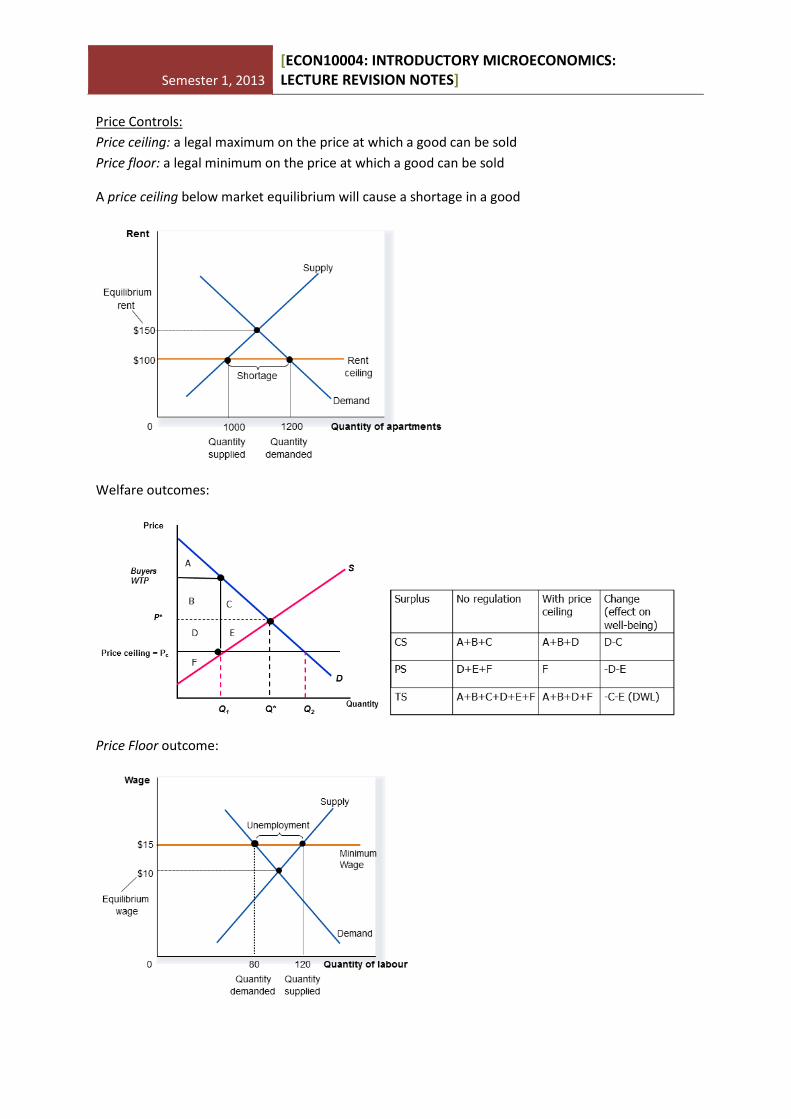
Price Controls:

Price ceiling: a legal maximum on the price at which a good can be sold

Price floor: a legal minimum on the price at which a good can be sold

A price ceiling below market equilibrium will cause a shortage in a good

Welfare outcomes:

Price Floor outcome:

Semester 1, 2013


Welfare outcome:

Subsidy: market outcomes:

Welfare outcomes:

Semester 1, 2013


Production Quota: Government intervention capping the amount of a good to be sold

Welfare outcomes:

Lecture Eight:

International Trade:

This model compares domestic price of a good without international trade and the price with trade

Without international trade, price would be set at market equilibrium, if Australian price is higher

than the international trade price there will be imports.

If the Australian price is lower than world price, Australians would lower their consumption because

domestic price would move to the higher world price, producers would also increase output.

To protect suppliers, the government can impose a tax called a tariff:

This creates a gain from Q* to QD

This causes a decrease in consumer

surplus but an increase in producer

surplus with an overall increase in

welfare from the extra quantity

supplied Q* to QS

Semester 1, 2013


The government can also impost an import quota which limits the quantity of a good produced

overseas which can be sold domestically

Lecture Nine:

Market failure can also be a failure to take account of all costs/benefits of a market transaction one

such failure is an externality.

Externalities are the ‘un-priced’ costs or benefits of an economic transaction. They arise when

economic agents engage in an activity that influences the wellbeing of a bystander who neither pays

for nor receives any compensation for the effect.

These effects may be positive or negative.

Markets which do not take into account these

externalities are considered socially inefficient

Negative externality:

Cost to society is higher than opportunity cost for

producers due to an adverse effect on bystanders

This increases world price to world

price plus tariff.

It increases quantity supplied

domestically and decreases imported

amount causing overall dead weight

loss in the triangles

This increases quantity supplied by

domestic suppliers causing a dead

weight loss in the triangles

Semester 1, 2013


eg. pollution. This makes the social cost curve above the supply curve, reflecting the social marginal

cost.

Q* is the competitive equilibrium however due to the effect of the negative externality, Q** is the

efficient quantity to be produced from the standpoint of society, this is the socially desirable level of

production, where SMC=SMB.

Due to the externality being negative, Q**<Q*

Positive externality:

Positive externalities give more benefits to society, making Q*<Q**

When individuals make decisions about how much of a product to buy, they ignore the external

benefits, considering only the private ones resulting in too few being bought. This means

competitive equilibrium is below the socially efficient level, creating a dead weight loss (market

failure).

How to achieve social efficiency:

Internalising the externality is an approach to have private decision makers take into account the

social costs/benefits of their decisions i.e. having these decisions affect them and hence they include

the cost/benefit in their decision-making process.

Government regulation can be used to give incentives, or have direct regulation to aid or limit

production.

Coase Theorem: trade between economic agents can achieve efficient solution (where negotiations

do not add too much extra cost)

Solutions for negative externalities:

For externalities that affect a certain group of people, negotiations can be had to come to an

agreement between parties (Coase Theorem)

The government can implement a production tax that equates PMC to SMC

The government can restrict production/emission levels by creating tradeable permits (e.g. pollution

permits, also creating a new market for pollution)

Solutions for positive externalities:

The government can create subsidies to encourage higher production/demand.

Lecture Ten:

Excludability: the property of a good whereby a person can be prevented from using it

Rivalry: the property of a good whereby one person’s use diminishes other people’s use

Free riders: a person who receives the benefit of a good but avoids paying for it

Private goods are excludable and rival.

Public goods:

Public goods are non-excludable and non-rival meaning there is no incentive for anyone to pay for

the good, thus these would be undersupplied if left to the private market compared to the socially

efficient outcome which would be a market failure e.g. national defence, police services, courts and

judges, storm water disposal etc.

Semester 1, 2013


For a public good, SMB>PMB as there is a positive externality however PMB<PMC therefore there is

no incentive to provide the good by any individual.

Solutions:

Government intervention:

- tax – the government can calculate SMB and SMC and decide upon the efficient quantity,

then they can finance the good’s provision through taxation

- assigning property rights

Lindahl tax: a tax in which each customer pays a different amount based on their WTP, it is the

consumer’s share of the total valuation multiplied by the cost of the good

Lecture 11:

Theory of the Firm:

- A firm is a collection of resources that is transformed into products demanded by consumers

- The costs at which a firm produces are governed by the available technology and cost of

resources

- The amount it produces and the prices at which it sells are influenced by the structure of the

markets in which it operates

- The difference between revenue received and costs incurred is profit

- The aim of a firm to maximise profit

Production function:

A firm incurs costs in the production of goods, the cost of producing a given quantity depends on the

production function and the price of inputs.

The production function is the relationship between the quantity of inputs used to make a good and

the quantity of the good produced.

A firm’s production function indicates the maximum level of output it can produce for any

combination of inputs this function can be expressed as Q = F(K, L), Q=output, K=Capital, L=Labour

The analysis of a production function can be looked at in the short-run or the long-run.

- Short-run: amount of inputs is fixed

- Long-run: the firm can vary all inputs

Short-run Production Function:

1. Average product of variable input: the

output per unit of input at each level

of production

2. Marginal product of variable input:

the output each additional unit of

input produces

Semester 1, 2013


When change in output declines, this is diminishing marginal product this is a property whereby the

marginal product of an input declines as the quantity of the input increases (e.g. workers

contributing less as more as hired)

To link production to cost, we convert the unit of

measurement from quantity produced to the cost of

producing each unit.

- Fixed Costs (FC): costs which do not vary with

quantity produced

- Variable Costs (VC): costs which vary with the

quantity of output produced

- Total Costs (TC): Total cost of production:

TFC+TVC

Lecture Twelve/Thirteen:

Measuring unit costs:

𝐴𝐹𝐶 = 𝑇𝑜𝑡𝑎𝑙 𝐹𝑖𝑥𝑒𝑑 𝐶𝑜𝑠𝑡𝑠

𝑄𝑢𝑎𝑛𝑡𝑖𝑡𝑦=

𝑇𝐹𝐶

𝑄

𝐴𝑉𝐶 = 𝑇𝑜𝑡𝑎𝑙 𝑉𝑎𝑟𝑖𝑎𝑏𝑙𝑒 𝐶𝑜𝑠𝑡𝑠


𝑇𝑉𝐶

𝑄

𝐴𝑇𝐶 = 𝑇𝑜𝑡𝑎𝑙 𝐶𝑜𝑠𝑡𝑠


𝑇𝐶

𝑄

𝑀𝐶 (𝑝𝑒𝑟 𝑢𝑛𝑖𝑡) = 𝐶ℎ𝑎𝑛𝑔𝑒 𝑖𝑛 𝑇𝑜𝑡𝑎𝑙 𝐶𝑜𝑠𝑡

𝐶ℎ𝑎𝑛𝑔𝑒 𝑖𝑛 𝑄𝑢𝑎𝑛𝑡𝑖𝑡𝑦=

∆𝑇𝐶

∆𝑄

Relationship between MP and MC:

If marginal product of a variable input is diminishing, then each extra input adds a smaller additional

amount to total output therefore needing more

labour to produce each extra unit of output as total

quantity increases

Marginal Costs: usually increasing with increased

quantity, or constant, if each additional unit of

variable input adds the same amount to total output

Average total costs: usually u-shaped because with

lower output, FC is the larger share of TC however

AFC decreases with increased output hence at higher

levels of output VC is the larger share or TC, or

decreases with quantity of output if FC is a very large

share of TC at any quantity of output

Semester 1, 2013


Relationship between MC and ATC:

MC intersects ATC at minimum of ATC because

- MC<ATC then ATC is decreasing

- MC>ATC then ATC is increasing

When MC=ATC the firm is efficient, it has achieved

productive efficiency

Long-run cost:

Long-run Average Cost Curve (LAC): defined as the

minimum average unit cost of producing at any level of

output when all inputs are variable. It is derived from a series of short run cost curves that represent

different factory sizes or amounts of fixed input.

The LAC is the lower section of all the combined SR ATC curves

The shape of the LAC is determined by the economies of scale

Lecture Fourteen:

Economic profit: 𝜋 = Total Revenue – Total Costs (implicit and explicit costs)

When there is a negative level of economic profit resources will leave the market as they would get a

better return in the next best use

If there is a zero level of economic profit there is no impact on resources as suppliers are no better

off by leaving or entering the market – this is the long-term outcome in a competitive market

If there is a positive level of economic profit resources will enter where possible as the rate of return

is higher than in current use

Profit Maximising decisions largely depend on the type or structure of the market. These features

include;

- Number and size distribution of firms

- Extent of product differentiation

Semester 1, 2013


- Barriers to entry/exit

- Price elasticity of demand

- Extent of information available to buyers and sellers

Market Structure (mature of the market) Market Conduct (decisions of firms made in respect to

price, output, advertising etc.) Market performance (Evaluation of decisions with respect to

factors such as profitability, efficiency, equity etc.)

Types of Markets:

Type of market: # of firms Entry Product Demand Curve

Perfect Competition:

Lots Unrestricted Homogeneous Perfectly elastic, price taker

Monopolistic Competition:

Many/Several Unrestricted Differentiated Relatively elastic, some price control

Oligopoly: Few Restricted Undifferentiated or differentiated

Relatively inelastic, depends on rivals’ actions

Monopoly: One Restricted/ Completely Blocked

Unique More inelastic than oligopoly, price maker

Perfectly competitive markets: No single buyer or seller has a negligible impact on the market price,

each buyer and seller takes the market price as given

Firm: Market:

Price setting decision is based off the cost-benefit principle by comparing marginal benefits with

marginal costs of supplying an additional unit of output, to maximise profits, MR=MC

Short-run economic profits: maximised at MR=MC, has positive economic profits at P>ATC, zero

economic profits at P=ATC and negative economic profits when P<ATC

Lecture Fifteen:

In a competitive market, profit maximisation occurs where P=MC

The two decisions, of what is the profit maximising quantity and at what prices should operations

cease, will determine a firm’s short-run supply curve.

Cease of operations:

- Shutdown: short run decision not to produce during a specific period of time because of

current market conditions

S

D

P

Quantity of firm Q*

P*

D=MR=AR

P

Quantity of firm

P* Market

Price

Semester 1, 2013


- Exit: long run decision to leave the market

The shutdown decision:

In the short run, the firm cannot avoid fixed costs, so these are treated as sunk costs, hence

opportunity cost of production is the firm’s variable cost

This means the shutdown decision would be made when revenue from production is less than

variable cost. –TR<TVC or P<AVC

Therefore the firm’s short run supply curve is the part of MC above minimum AVC

While the firm will make a loss when P<ATC, loss minimising would still exist by producing goods

when AVC<P<ATC.

The exit decision:

In the long run, all of a firm’s costs are variable; therefore the firm’s opportunity cost of production

is their total costs. Therefore the exit decision of a firm would be when revenue is less that total

costs –TR<TC or P<ATC

The short run market supply curve shows the amount of output the industry will produce in the

short run for each possible price. It is the horizontal summation of all the firms’ supply curves

For the long run, there is the assumption that there are no barriers to entry/exit and all firms have

access to the same technology meaning the decision to enter is based on profit incentive. If existing

firms are profitable, more firms will enter and increased supply will drive down price and profit. If

existing firms are making losses, firms will exit, decreasing supply and driving prices and profits up.

Semester 1, 2013


Market equilibrium in a competitive market:

Short run: # of firms is fixed, firms make economic profit at P>ATC, 0 at P=ATC or losses at P<ATC

Long run: # of firms may vary with no barriers to entry or exit, firms can only earn 0 profit P=ATC

Lecture Sixteen:

Monopoly:

Welfare implications of a monopoly:

Semester 1, 2013


To find the profit maximising price and quantity for a monopoly, use the demand curve, make P the

subject, double the gradient to find the marginal revenue curve and equated MR=MC.

Monopolies have market power, because they can charge a higher price and produce a lower output

than if the conditions were of perfect competition, this means they are producing an inefficient level

of output.

The inefficiency is measure by dead weight loss, which is a loss of both consumer and producer

surplus creating the social cost of market power

Some companies win market power by being innovative and adaptable/more efficient than others or

meeting consumers’ needs better, in this case consumers are the net beneficiaries in situations

where a firm succeeds in becoming the dominant player through lower prices and better products.

These firms may be efficient in the long run, but trade off short run allocative efficiency.

Market power is measured by the

extent to which the profit

maximising price exceeds marginal

cost i.e. mark-up over marginal

cost

The extent to which a firm can

price its product above marginal

cost depends largely on the price

elasticity of demand for the

product.

In reality, studies have indicated that manages determine prices based on a reliance of cost

approach or demand, however most managers appear to use some type of inverse price elasticity

rule which involves both demand and cost in calculating mark-up.

Government policy towards monopolies:

- Competition laws

- Price regulation

- Government ownership

Semester 1, 2013


Natural monopolies can achieve very low costs

when producing large quantities and have the

potential to charge high prices to earn large

economic profits. E.g. natural gas, electricity

In Australia, state regulatory commissions often

set prices for natural monopolies, this can be at

P=ATC or by using two part pricing where

consumers are charged a fixes component to

cover AFC and a variable component to cover

MC.

Lecture Seventeen: notes not on LMS

Lecture Eighteen:

Firms with market power can set one price for all customers by applying the profit maximising rule,

however by setting a high price, they only sell goods to customers with a high willingness to pay

(WTP), and these customers retain consumer surplus.

Additionally, the firm loses sales to other customers, resulting in dead weight loss (DWL)

Therefore the price chosen is a trade-off between charging a higher price to customers with a high

WTP and charging a lower price and selling more of the good.

Non-uniform Pricing/Price Discrimination:

Firms can use information about individual customers’ WTP to increase prices by charging different

prices based off the WTP.

Price Discrimination: is the main form of non-uniform pricing in which the same product is sold at

different prices to different customers, where prices do not relate to cost of production.

The objective of this is to target different WTP of customers so as to capture their consumer surplus

and increase profit. There are three main types of price discrimination; first, second and third degree

price discrimination.

First degree price discrimination: is charging each customer their maximum WTP for each unit of the

product bought, thus causing the entire consumer surplus to turn into profit.

This is also known as perfect price discrimination; the firm’s marginal revenue curve will be the

demand curve.

(Second degree price discrimination: is charging different prices for different quantities of a good. )

Third degree price discrimination: segmenting buyers into groups on the basis of WTP and charging

different prices for each group, also known as multi-market price discrimination.

To calculate the optimal third degree price discrimination, we find the profit maximising price for

each segment of the market separately, then compare with a uniform price over the whole market

to see if there is incentive for price discrimination.

Two-part pricing: charging buyers a fixed fee as well as an additional usage fee for each unit of the

product consumed.

Semester 1, 2013


To calculate the optimal two-part pricing, we set usage price to marginal cost (MC) with a fixed fee

of the consumer surplus.

Bundling: charging buyers one price for two or more products sold as a package, rather than

charging a separate price for each one individually.

To calculate WTP for bundles, we add the value the consumer places on each product together, then

find the profit maximising price and compare to profit if each were sold separately.

For price discrimination to work, three conditions must be met:

1. The firm must have market power to charge above competitive price

2. Customers must differ in their price sensitivity – different WTP levels

3. Firms must be able to prevent or limit resale

Lecture Nineteen:

Pricing decisions:

Competitive market: P=MC, zero profits in long run, P=ATC

Monopoly: MR=MC and set price at what consumers are willing to pay, possible to earn profit in

long-run but produces at an inefficient level, causing DWL

Characteristics of monopolistic competition:

- Many buyers and sellers

- Product differentiation but products are close substitutes

- Relatively elastic demand curve

- No barriers to entry

- Market structure lies between perfect competition and a monopoly

The main source of market power in with monopolistic competition is product differentiation which

aims to change the consumers’ view that all products are perfect substitutes by creating differences

in quality, features, brands etc. This means consumers cannot simply switch to another supply and

receive the exact same product.

Pricing decisions:

In the short run, firms can make economic profits where P>ATC, demand is relatively elastic where

there are many good substitutes and profit is maximised when MR=MC

In the long run, as new firms are attracted to the industry by profit opportunities, the existing firms’

demand will decrease and become more elastic, resulting in less market power. The firms’ outputs

and prices will fall and industry output will rise. There is no economic profit due to no barriers of

entry so P=ATC, however there is still some monopoly power so P>MC.

This means there are two long run equilibrium characteristics for monopolistic competition, either as

with a monopoly where P>MC with profit maximisation at MR=MC or as with a competitive market

where P=ATC, due to free entry driving economic profit to zero.

Semester 1, 2013


The result of new firms entering a market will be that demand for existing suppliers will be reduced

as well as an increase in elasticity because of the availability of more substitutes.

Monopolistic vs Perfect competition:

Perfect competition: No excess capacity in the long run as p=ATC causing everyone to produce at the

efficient level. P=MC

Monopolistic competition: Higher average cost due to inefficient output. P>MC due to market

power, creating higher profits but also resulting in DWL

Effects of competition:

Due to firms needing to differentiate their products, there is more incentive for imitation or

innovation. There is a greater degree of competition, making it harder for firms to earn positive

profits in the long run.

Firms can differentiate products by creating something with the fewest number of close substitutes,

by developing the product, advertising or creating a brand name and image etc.

Lecture Twenty:

Perfect competition: P=MC, free entry/exit, 0 long run profit

Monopoly: P>MC, barriers to entry, positive long run profit

Monopolistic competition: M>MC, product differentiation, some market power, free entry/exit, 0

long run profits

Semester 1, 2013


Oligopoly: P>MC, high barriers to entry, substantial market power, limited by firm rivalry, positive

profits in long run

Oligopoly:

- A few firms account for most/total industry production

- Products may or may not be differentiated

- Concentrated markets because of substantial barriers to entry e.g. economies of scale,

patents, funding, market reputation etc.

Market Concentration: concentration ratio: measure the size of the top firms in an industry as a

proportion of the total industry size e.g. four firm concentration ratio is the % of industry sales

accounted for by the top four firms. The higher the ratio, the more concentrated the industry.

Strategic consideration: Decision-making in an oligopolistic firm is complicated because of strategic

considerations. Each firm must carefully consider how its actions will affect rival firms and how they

are likely to react.

A key feature of oligopoly is the tension between cooperation and self-interest – a group of

oligopolists are best off cooperating and acting as a monopolist by producing a smaller quantity and

charging P>MC however because each firm cares only about their own profit, there is incentives to

increase output.

Duopoly: an oligopoly with only two sellers

Nash Equilibrium: a situation in which economic actors interacting with one another choose their

best strategy given the strategies that all the others have chosen. With a NE, there is no incentive for

a firm to increase/decrease production.

Game Theory:

Game Theory is a study of strategic situations in which decision-makers need to anticipate other

players’ decisions before best knowing how to behave themselves.

Rules:

- Set of platers

- Set of strategic options available to each player

- Payoffs of each player for all possible combinations of strategies pursued by all the players

- Assumption that all players are rational (wish to make profit)

Strategy: a strategy for a player is a complete plan for the actions they will take at each stage of the

game

Key Elements:

- Payoffs: a payoff is the number which represents the well-being outcome for that player

- Equilibrium: the predicted outcome for the game subject to the requirement that each

player chooses a strategy that is the ‘best response’ to the strategies of the other players

Semester 1, 2013


- Strategic decisions: those in which each player must decide how the other will respond in

deciding what actions to take

Game table: simultaneous games

Game tree: sequential games

Dominant strategy: a strategy which, regardless of the actions of the other players, always gives a

player a higher payoff than the other available strategies

Lecture Twenty-One:

Nash Equilibrium: choice of strategy for each player such that their strategy achieves the highest

possible payoff given all other players and choosing their ‘best response’ strategies

Rules:

1. If you have a dominant strategy, use it

2. Never play a dominated strategy

3. If your opponent has a dominant strategy or dominated strategy, this may reveal your own

best strategy

Lecture Twenty-Two:

Sequential move games are games in which one player moves first, and the second mover observes

the action taken by the first mover before it decides what action to take

To determine the moves made by players in a sequential game, we use a process called backward

induction

The equilibrium found through a sequential game is known as a rollback equilibrium

Rollback equilibrium is the actions that rational players would take – the choice of strategy for each

player such that each player chooses at each decision node the action that is payoff maximising

given all other players choose optimal actions at all subsequent decision nodes in the game tree

1. Look ahead and reason back, using the principle of backward induction to think about what

other players will do and hence decide one’s own best choice of action

2. Order matters, being in a sequential game can alter payoff compared to simultaneous game

Strategic moves:

A move that influences the other person’s choice in a manner favourable to one’s self, by affecting

the other person’s expectations of how one’s self will behave, i.e. constraining the other players

choice by constraining one’s own behaviour.

Lecture Twenty-Three:

Barriers to entry are an important source of monopoly power and profits, these can arise natural –

economies of scale, patents etc. or firms can deter entry by making strategic moves. They can do so

by convincing any potential competitor that entry will be unprofitable, but this involves a

commitment.

For a strategy to be effective, it must be credible, and must change the payoffs so your rival changes

their behaviour in a way which benefits you

econ10004: introductory microeconomics: lecture revision notes

Documents