econ 424/amath 462 hypothesis testing in the cer modelecon 424/amath 462 hypothesis testing in the...

Econ 424/Amath 462

Hypothesis Testing in the CER Model

Eric Zivot

July 23, 2013

Hypothesis Testing

1. Specify hypothesis to be tested

0 : null hypothesis versus. 1 : alternative hypothesis

2. Specify significance level of test

level = Pr(Reject 0|0 is true)

3. Construct test statistic, from observed data

4. Use test statistic to evaluate data evidence regarding 0

| | is big ⇒ evidence against 0| | is small ⇒ evidence in favor of 0

Decide to reject 0 at specified significance level if value of falls in therejection region

∈ rejection region ⇒ reject 0

Usually the rejection region of is determined by a critical value, such that

| | ⇒ reject 0| | ≤ ⇒ do not reject 0

Decision Making and Hypothesis Tests

RealityDecision 0 is true 0 is false

Reject 0 Type I error No errorDo not reject 0 No error Type II error

Significance Level of Test

level = Pr(Type I error)

Pr(Reject 0|0 is true)

Goal: Constuct test to have a specified small significance level

level = 5% or level = 1%

Power of Test

1− Pr(Type II error)= Pr(Reject 0|0 is false)

Goal: Construct test to have high power

Problem: Impossible to simultaneously have level ≈ 0 and power ≈ 1 As level→ 0 power also → 0

Hypothesis Testing in CER Model

= + = 1 · · · ; = 1 · · · ∼ iid (0 2 )

cov( ) = cor( ) =

cov( ) = 0 6= for all

• Test for specific value

0 : = 0 vs. 1 : 6= 00 : = 0 vs. 1 : 6= 00 : = 0 vs. 1 : 6= 0

• Test for sign

0 : = 0 vs. 1 : 0 or 0

0 : = 0 vs. 1 : 0 or 0

• Test for normal distribution

0 : ∼ iid ( 2 )1 : ∼ not normal

• Test for no autocorrelation

0 : = corr( −) = 0, 1

1 : = corr( −) 6= 0 for some

• Test of constant parameters

0 : and are constant over entire sample

1 : or changes in some sub-sample

Definition: Chi-square random variable and distribution

Let 1 be iid (0 1) random variables. Define

= 21 + · · ·+ 2

Then

∼ 2()

= degrees of freedom (d.f.)

Properties of 2() distribution

0

[] =

2()→ normal as →∞

R functions

rchisq(): simulate data

dchisq(): compute density

pchisq(): compute CDF

qchisq(): compute quantiles

Definition: Student’s t random variable and distribution with degreesof freedom

∼ (0 1) ∼ 2()

and are independent

=q

∼

= degrees of freedom (d.f.)

Properties of distribution:

[ ] = 0

skew( ) = 0

kurt( ) =3 − 6 − 4

4

→ (0 1) as →∞ ( ≥ 60)

R functions

rt(): simulate data

dt(): compute density

pt(): compute CDF

qt(): compute quantiles

Test for Specific Coefficient Value

0 : = 0 vs. 1 : 6= 0

1. Test statistic

=0=

− 0cSE()Intuition:

• If =0 ≈ 0 then ≈ 0 and 0 : = 0 should not be rejected

• If |=0 | 2, say, then is more than 2 values of cSE() away from0 This is very unlikely if = 0 so 0 : = 0 should be rejected.

Distribution of t-statistic under 0

Under the assumptions of the CER model, and 0 : = 0

=0=

− 0cSE() ∼ −1

where

=1

X=1

cSE() = √

=

vuuut 1

− 1

X=1

( − )2

−1 = Student’s t distribution with

− 1 degrees of freedom (d.f.)

Remarks:

• −1 is bell-shaped and symmetric about zero (like normal) but with fattertails than normal

• d.f. = sample size - number of estimated parameters. In CER model thereis one estimated parameter, so df = − 1

• For ≥ 60 −1 ' (0 1). Therefore, for ≥ 60

=0=

− 0cSE() ' (0 1)

2. Set significance level and determine critical value

Pr(Type I error) = 5%

Test has two-sided alternative so critical value, 025 is determined using

Pr(|−1| 025) = 005⇒ 025 = −−1025 =

−1975

where −1975 = 975% quantile of Student-t distribution with − 1 degrees of

freedom.

3. Decision rule:

reject 0 : = 0 in favor of 1 : 6= 0 if

|=0 | 975

Useful Rule of Thumb:

If ≥ 60 then 975 ≈ 2 and the decision rule is

Reject 0 : = 0 at 5% level if

|=0 | 2

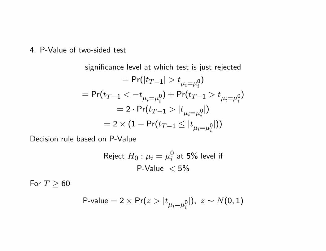
4. P-Value of two-sided test

significance level at which test is just rejected

= Pr(|−1| =0)

= Pr(−1 −=0 ) + Pr(−1 =0)

= 2 · Pr(−1 |=0 |)

= 2× (1− Pr(−1 ≤ |=0 |))

Decision rule based on P-Value

Reject 0 : = 0 at 5% level if

P-Value 5%

For ≥ 60

P-value = 2× Pr( |=0 |) ∼ (0 1)

Tests based on CLT

Let denote an estimator for . In many cases the CLT justifies the asymptoticnormal distribution

∼ ( se()2)

Consider testing

0 : = 0 vs. 1 : 6= 0

Result: Under 0

=0 = − 0cse() ∼ (0 1)

for large sample sizes.

Example: In the CER model, for large enough the CLT gives

∼ ( ()2)

() =√2

and

∼ ( ()2)

() =

q1− 2√

Rule-of-thumb Decision Rule

Let Pr(Type I error)= 5% Then reject

0 : = 0 vs. 1 : 6= 0

at 5% level if

|=0| =¯¯ − 0cse()

¯¯ 2

Relationship Between Hypothesis Tests and Confidence Intervals

0 : = 0 vs. 1 : 6= 0level = 5%

975 = −1975 ≈ 2 for 60

=0=

− 0cSE()Reject at 5% level if |=0 | 2

Approximate 95% confidence interval for

= ±2 · cSE()= [ − 2 · cSE() + 2 · cSE()]

Decision: Reject 0 : = 0 at 5% level if 0 does not lie in 95% confidence

interval.

Test for Sign

0 : = 0 vs. 1 : 0

1. Test statistic

=0 =cSE()

Intuition:

• If =0 ≈ 0 then ≈ 0 and 0 : = 0 should not be rejected

• If =0 0, then this is very unlikely if = 0 so 0 : = 0 vs.1 : 0 should be rejected.



One-sided critical value is determined using

Pr(−1 05) = 005

⇒ 05 = −195

where −195 = 95% quantile of Student-t distribution with − 1 degrees of

freedom.

3. Decision rule:

Reject 0 : = 0 vs. 1 : 0 at 5% level if

=0 −195

Useful Rule of Thumb:

If ≥ 60 then −195 ≈ 95 = 1645 and the decision rule is

Reject 0 : = 0 vs. 1 : 0 at 5% level if

=0 1645

4. P-Value of test


= Pr(−1 =0)

= Pr( =0) for ≥ 60

Test for Normal Distribution

0 : ∼ iid ( 2)1 : ∼ not normal

1. Test statistic (Jarque-Bera statistic)

JB =

6

Ã[skew

2+(dkurt− 3)2

4

!See R package tseries function jarque.bera.test

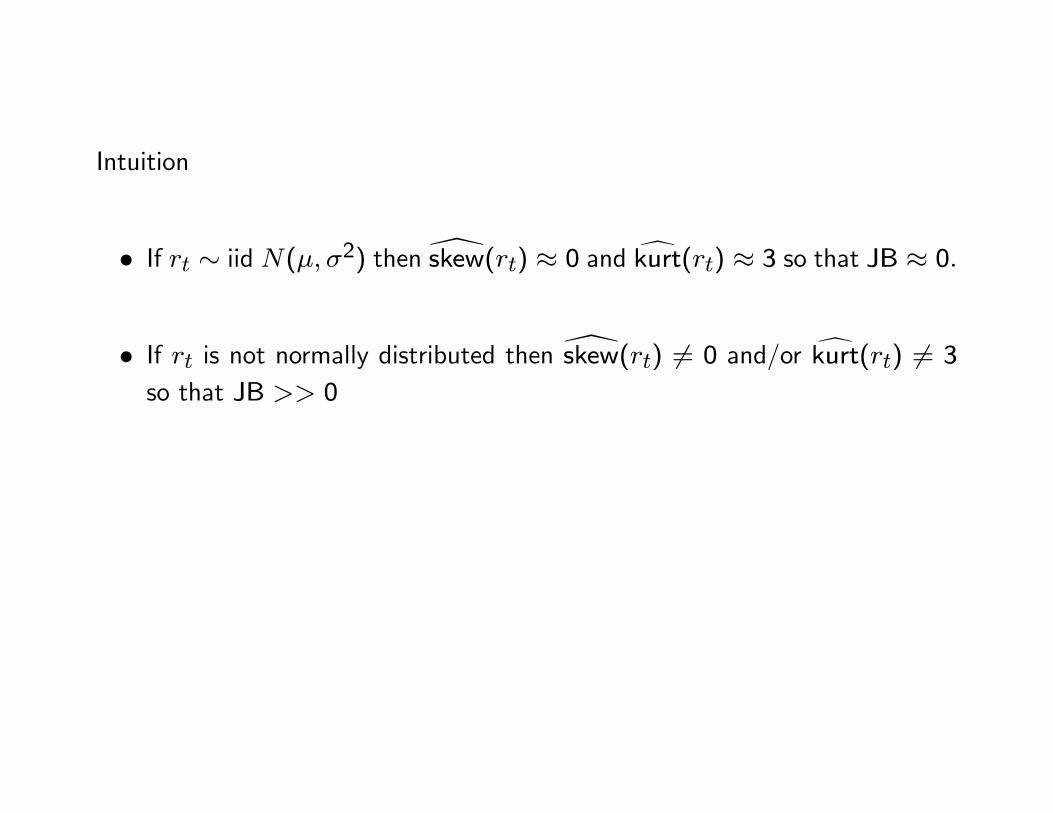
Intuition

• If ∼ iid ( 2) then[skew() ≈ 0 and dkurt() ≈ 3 so that JB ≈ 0• If is not normally distributed then [skew() 6= 0 and/or dkurt() 6= 3

so that JB 0

Distribution of JB under 0

If 0 : ∼ iid ( 2) is true then

JB ∼ 2(2)

where 2(2) denotes a chi-square distribution with 2 degrees of freedom (d.f.).



Critical value is determined using

Pr(2(2) ) = 005

⇒ = 2(2)95 ≈ 6

where 2(2)

95 ≈ 6 ≈ 95% quantile of chi-square distribution with 2 degrees offreedom.

3. Decision rule:

Reject 0 : ∼ iid ( 2)at 5% level if JB 6

4. P-Value of test


= Pr(2(2) JB)

Test for No Autocorrelation

Recall, the j lag autocorrelation for is

= cor( −)

=cov( −)var()

Hypotheses to be tested

0 : = 0, for all = 1

1 : 6= 0 for some

1. Estimate using sample autocorrelation

=

1−1

P=+1( − )(− − )

1−1

P=1( − )2

Result: Under 0 : = 0 for all = 1 if is large then

∼ µ01

¶for all ≥ 1

SE() =1√

2. Test Statistic

=0 =

SE()=

1√=√

and 95% confidence interval

± 2 ·1√

3. Decision rule

Reject 0 : = 0 at 5% levelif |=0| =

¯√

¯ 2

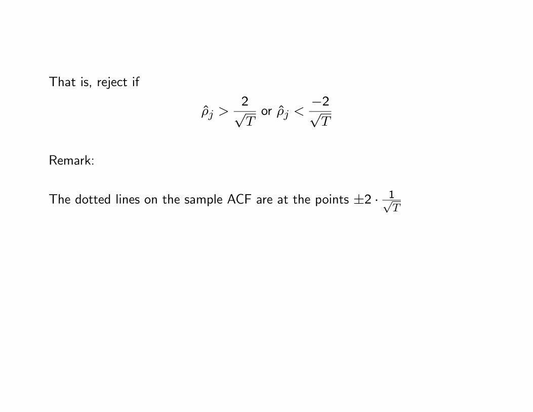
That is, reject if

2√or

−2√

Remark:

The dotted lines on the sample ACF are at the points ±2 · 1√

Diagnostics for Constant Parameters

0 : is constant over time vs. 1 : changes over time



Remarks

• Formal test statistics are available but require advanced statistics

— See R package strucchange

• Informal graphical diagnostics: Rolling estimates of and

Rolling Means

Idea: compute estimate of over rolling windows of length

() =1

−1X=0

−

=1

( + −1 + · · ·+ −+1)

R function (package zoo)

rollapply

If 0 : is constant is true, then () should stay fairly constant overdifferent windows.

If 0 : is constant is false, then () should fluctuate across differentwindows

Rolling Variances and Standard Deviations

Idea: Compute estimates of 2 and over rolling windows of length

2() =1

− 1

−1X=0

(− − ())2

() =q2()



Rolling Covariances and Correlations

Idea: Compute estimates of and over rolling windows of length

() =1

− 1

−1X=0

(− − ())(− − ())

() =()

()()



econ 424/amath 462 hypothesis testing in the cer modelecon 424/amath 462 hypothesis testing in the...

Documents