Project Number 288094

eCOMPASSeCO-friendly urban Multi-modal route PlAnning Services for mobile uSers

STREPFunded by EC, INFSO-G4(ICT for Transport) under FP7

eCOMPASS – TR – 004

On the Hardness of Network Design forBottleneck Routing Games

Dimitris Fotakis, Alexis C. Kaporis, Thanasis Lianeas, Paul G. Spirakis

July 2012

On the Hardness of Network Design for Bottleneck Routing Games?

Dimitris Fotakis1, Alexis C. Kaporis2, Thanasis Lianeas1, and Paul G. Spirakis3,4

1 School of Electrical and Computer Engineering, National Technical University of Athens, 15780 Athens, Greece.2 Department of Information and Communication Systems Engineering, University of the Aegean, Greece.

3 Department of Computer Engineering and Informatics, University of Patras, 26500 Patras, Greece.4 Research Academic Computer Technology Institute, N. Kazantzaki Str., University Campus, 26500 Patras, Greece.

Email: fotakis@cs.ntua.gr, kaporisa@gmail.com, tlianeas@mail.ntua.gr,spirakis@cti.gr

Abstract. In routing games, the selfish behavior of the players may lead to a degradation of the networkperformance at equilibrium. In more than a few cases however, the equilibrium performance can be signif-icantly improved if we remove some edges from the network. This counterintuitive fact, widely known asBraess’s paradox, gives rise to the (selfish) network design problem, where we seek to recognize routinggames suffering from the paradox, and to improve their equilibrium performance by edge removal. In thiswork, we investigate the computational complexity and the approximability of the network design problemfor non-atomic bottleneck routing games, where the individual cost of each player is the bottleneck costof her path, and the social cost is the bottleneck cost of the network, i.e. the maximum latency of a usededge. We first show that bottleneck routing games do not suffer from Braess’s paradox either if the networkis series-parallel, or if we consider only subpath-optimal Nash flows. On the negative side, we prove thateven for games with strictly increasing linear latencies, it is NP-hard not only to recognize instances suffer-ing from the paradox, but also to distinguish between instances for which the Price of Anarchy (PoA) candecrease to 1 and instances for which the PoA cannot be improved by edge removal, even if their PoA isas large as Ω(n0.121). This implies that the network design problem for linear bottleneck routing games isNP-hard to approximate within a factor of O(n0.121−ε), for any constant ε > 0. The proof is based on arecursive construction of hard instances that carefully exploits the properties of bottleneck routing games,and may be of independent interest. On the positive side, we present an algorithm for finding a subnetworkthat is almost optimal w.r.t. the bottleneck cost of its worst Nash flow, when the worst Nash flow in thebest subnetwork routes a non-negligible amount of flow on all used edges. We show that the running time isessentially determined by the total number of paths in the network, and is quasipolynomial when the numberof paths is quasipolynomial.

? This work was partially supported by an NTUA Basic Research Grant (PEBE 2009), by the Greek GSR project Algo-rithmic Game Theory/THALIS, by the ERC project RIMACO, and by the EU-FP7 Project e-Compass.

1 Introduction

An typical instance of a non-atomic bottleneck routing game consists of a directed network, withan origin s and a destination t, where each edge is associated with a non-decreasing function thatdetermines the edge’s latency as a function of its traffic. A rate of traffic is controlled by an infinitepopulation of players, each willing to route a negligible amount of traffic through an s − t path.The players are non-cooperative and selfish, and seek to minimize the maximum edge latency, a.k.a.the bottleneck cost of their path. Thus, the players reach a Nash equilibrium flow, or simply a Nashflow, where they all use paths with a common locally minimum bottleneck cost. Bottleneck routinggames and their variants have received considerable attention due to their practical applications incommunication networks (see e.g., [6, 3] and the references therein).

Previous Work and Motivation. Every bottleneck routing game is known to admit a Nash flowthat is optimal for the network, in the sense that it minimizes the maximum latency on any used edge,a.k.a. the bottleneck cost of the network (see e.g., [3, Corollary 2]). On the other hand, bottleneckrouting games usually admit many different Nash flows, some with a bottleneck cost quite far from theoptimum. Hence, there has been a considerable interest in quantifying the performance degradationdue to the players’ non-cooperative and selfish behavior in (several variants of) bottleneck routinggames. This is typically measured by the Price of Anarchy (PoA) [12], which is the ratio of thebottleneck cost of the worst Nash flow to the optimal bottleneck cost of the network.

Simple examples (see e.g., [7, Figure 2]) demonstrate that the PoA of bottleneck routing gameswith linear latency functions can be as large as Ω(n), where n is the number of vertices of the network.For atomic splittable bottleneck routing games, where the population of players is finite, and eachplayer controls a non-negligible amount of traffic which can be split among different paths, Banner andOrda [3] observed that the PoA can be unbounded, even for very simple networks, if the players havedifferent origins and destinations and the latency functions are exponential. On the other hand, Bannerand Orda proved that if the players use paths that, as a secondary objective, minimize the number ofbottleneck edges, then all Nash flows are optimal. For a variant of non-atomic bottleneck routinggames, where the social cost is the average (instead of the maximum) bottleneck cost of the players,Cole, Dodis, and Roughgarden [7] proved that the PoA is 4/3, if the latency functions are affine and asubclass of Nash flows, called subpath-optimal Nash flows, is only considered. Subsequently, Mazalovet al. [15] studied the inefficiency of the best Nash flow under this notion of social cost.

For atomic unsplittable bottleneck routing games, where each player routes a unit of traffic througha single s − t path, Banner and Orda [3] proved that for polynomial latency functions of degree d,the PoA is O(md), where m is the number of edges of the network. On the other hand, Epstein,Feldman, and Mansour [8] proved that for series-parallel networks with arbitrary latency functions, allNash flows are optimal. Subsequently, Busch and Magdon-Ismail [5] proved that the PoA of atomicunsplittable bottleneck routing games with identity latency functions can be bounded in terms ofnatural topological properties of the network. In particular, they proved that the PoA of such gamesis bounded from above by O(l + log n), where l is the length of the longest s − t path, and byO(k2 + log2 n), where k is length of the longest circuit.

With the PoA of bottleneck routing games so high and crucially depending on topological prop-erties of the network, a natural approach to improving the performance at equilibrium is to exploit theessence of Braess’s paradox [4], namely that removing some edges may change the network topology(e.g., it may decrease the length of the longest path or cycle), and significantly improve the bottleneckcost of the worst Nash flow (see e.g., Fig. 1). This approach gives rise to the (selfish) network designproblem, where we seek to recognize bottleneck routing games suffering from the paradox, and toimprove the bottleneck cost of the worst Nash flow by edge removal. In particular, given a bottleneck

1

Fig. 1. An example of Braess’s paradox for bottleneck routing games. We consider a routing instance with identity latencyfunctions and a unit of traffic to be routed from s to t. The worst Nash flow, in (a), routes all flow through the path (s, u, v, t),and has a bottleneck cost of 1. On the other hand, the optimal flow routes 1/2 unit through the path (s, u, t) and 1/2 unitthrough the path (s, v, t), and has a bottleneck cost of 1/2. Hence, PoA = 2. In the subnetwork (b), obtained by removingthe edge (u, v), we have a unique Nash flow that coincides with the optimal flow, and thus the PoA becomes 1. Hence thenetwork on the left is paradox-ridden, and the network on the right is the best subnetwork of it.

routing game, we seek for the best subnetwork, namely, the subnetwork for which the bottleneck costof the worst Nash flow is best possible. In this setting, one may distinguish two extreme classes of in-stances: paradox-free instances, where edge removal cannot improve the bottleneck cost of the worstNash flow, and paradox-ridden instances, where the bottleneck cost of the worst Nash flow in the bestsubnetwork is equal to the optimal bottleneck cost of the original network (see also [17, 10]).

The approximability of selective network design, a generalization of network design where wecannot remove certain edges, was considered by Hou and Zhang [11]. For atomic unsplittable bottle-neck routing games with a different traffic rate and a different origin and destination for each player,they proved that if the latency functions are polynomials of degree d, it is NP-hard to approximateselective network design within a factor of O(md−ε), for any constant ε > 0. Moreover, for atomick-splittable bottleneck routing games with multiple origin-destination pairs, they proved that selectivenetwork design is NP-hard to approximate within any constant factor.

However, a careful look at the reduction of [11] reveals that their strong inapproximability resultscrucially depend on both (i) that we can only remove certain edges from the network, so that thesubnetwork actually causing a high PoA cannot be destroyed, and (ii) that the players have differentorigins and destinations (and also are atomic and have different traffic rates). As for the importanceof (ii), in a different setting, where the players’ individual cost is the sum of edge latencies on theirpath and the social cost is the bottleneck cost of the network, it is known that Braess’s paradox canbe dramatically more severe for instances with multiple origin-destination pairs than for instanceswith a single origin-destination pair. More precisely, Lin et al. [13] proved that if the players havea common origin and destination, the removal of at most k edges from the network cannot improvethe equilibrium bottleneck cost by a factor greater than k + 1. On the other hand, Lin et al. [14]presented an instance with two origin-destination pairs where the removal of a single edge improvesthe the equilibrium bottleneck cost by a factor of 2Ω(n). Therefore, both at the technical and at theconceptual level, the inapproximability results of [11] do not really shed light on the approximabilityof the (simple, non-selective) network design problem in the simplest, and most interesting, setting ofnon-atomic bottleneck routing games with a common origin-destination pair for all players.

Contribution. Hence, in this work, we investigate the approximability of the network design problemfor the simplest, and seemingly easier to approximate, variant of non-atomic bottleneck routing games(with a single origin-destination pair). Our main result is that network design is hard to approximatewithin reasonable factors, and holds even for the special case of strictly increasing linear latencies. Tothe best of our knowledge, this is the first work that investigates the impact of Braess’s paradox andthe approximability of the network design problem for the basic variant of bottleneck routing games.

2

In Section 3, we use techniques similar to those in [8, 7], and show that bottleneck routing gamesdo not suffer from Braess’s paradox either if the network is series-parallel, or if we consider onlysubpath-optimal Nash flows.

On the negative side, we employ, in Section 4, a reduction from the 2-Directed Disjoint Pathsproblem, and show that for linear bottleneck routing games, it is NP-hard to recognize paradox-ridden instances (Lemma 1). In fact, the reduction shows that it is NP-hard to distinguish betweenparadox-ridden instances and paradox-free instances, even if their PoA is equal to 4/3, and thus, it isNP-hard to approximate the network design problem within a factor less than 4/3.

In Section 5, we apply essentially the same reduction, but in a recursive way, and obtain a muchstronger inapproximability result. In particular, we assume the existence of a γ-gap instance, whichestablishes that network design is inapproximable within a factor less than γ, and show that the con-struction of Lemma 1, but with some edges replaced by copies of the gap instance, amplifies theinapproximability threshold by a factor of 4/3, while it increases the size of the network by roughlya factor of 8 (Lemma 2). Therefore, starting from the 4/3-gap instance of Lemma 1, and recursivelyapplying this construction a logarithmic number times, we show that it is NP-hard to approximatethe network design problem for linear bottleneck routing games within a factor of O(n0.121−ε), forany constant ε > 0. An interesting technical point is that we manage to show this inapproximabil-ity result, even though we do not know how to efficiently compute the worst equilibrium bottleneckcost of a given subnetwork. Hence, our reduction uses a certain subnetwork structure to identify goodapproximations to the best subnetwork. To the best of our knowledge, this is the first rime that a sim-ilar recursive construction is used to amplify the inapproximability threshold of the network designproblem, and of any other optimization problem related to selfish routing.

In Section 6, we consider latency functions that satisfy a Lipschitz condition, and present analgorithm for finding a subnetwork that is almost optimal w.r.t. the bottleneck cost of its worst Nashflow, when the worst Nash flow in the best subnetwork routes a non-negligible amount of flow onall used edges. The algorithm is based on Althofer’s Sparcification Lemma [1], and is motivated byits recent application to network design for additive routing games [10]. For any constant ε > 0, thealgorithm computes a subnetwork and an ε/2-Nash flow whose bottleneck cost is within an additiveterm of O(ε) from the worst equilibrium bottleneck cost in the best subnetwork. The running time isroughly |P|poly(logm)/ε2 , and is quasipolynomial, when the number |P| of paths is quasipolynomial.

Other Related Work. Considerable attention has been paid to the approximability of the networkdesign problem for additive routing games, where the players seek to minimize the sum of edge laten-cies on their path, and the social cost is the total latency incurred by the players. In fact, Roughgarden[17] first introduced the selfish network design problem in this setting, and proved that it is NP-hardto recognize paradox-ridden instances. Roughgarden also proved that it is NP-hard to approximatethe network design problem for additive routing games within a factor less than 4/3 for affine laten-cies, and less than bn/2c for general latencies. For atomic unsplittable additive routing games withweighted players, Azar and Epstein [2] proved that network design is NP-hard to approximate withina factor less than 2.618, for affine latencies, and less than dΘ(d), for polynomial latencies of degree d.

On the positive side, Milchtaich [16] proved that non-atomic additive routing games on series-parallel networks do not suffer from Braess’s paradox. Fotakis, Kaporis, and Spirakis [10] provedthat we can efficiently recognize paradox-ridden instances when the latency functions are affine, andall, but possibly a constant number of them, are strictly increasing. Moreover, applying Althofer’sSparsification Lemma [1], they gave an algorithm that approximates network design for affine additiverouting games within an additive term of ε, for any constant ε > 0, in time that is subexponential ifthe total number of s− t paths is polynomial and all paths are of polylogarithmic length.

3

2 Model, Definitions, and Preliminaries

Routing Instances. A routing instance is a tuple G = (G(V,E), (ce)e∈E , r), where G(V,E) is adirected network with an origin s and a destination t, ce : [0, r] 7→ IR≥0 is a continuous non-decreasinglatency function associated with each edge e, and r > 0 is the traffic rate entering at s and leaving att. We let n ≡ |V | and m ≡ |E|, and let P denote the set of simple s− t paths in G. A latency functionce(x) is linear if ce(x) = aex, for some ae > 0, and affine if ce(x) = aex+ be, for some ae, be ≥ 0.We say that a latency function ce(x) satisfies the Lipschitz condition with constant ξ > 0, if for allx, y ∈ [0, r], |ce(x)− ce(y)| ≤ ξ|x− y|.Subnetworks and Subinstances. Given a routing instance G = (G(V,E), (ce)e∈E , r), any subgraphH(V,E′), E′ ⊆ E, obtained from G by edge deletions, is a subnetwork of G. H has the same origins and destination t as G, and the edges of H have the same latency functions as in G. Each instanceH = (H(V,E′), (ce)e∈E′ , r), where H(V,E′) is a subnetwork of G(V,E), is a subinstance of G.Flows. A (G-feasible) flow f is a non-negative vector indexed by P so that

∑p∈P fp = r. For a flow

f and each edge e, we let fe =∑

p:e∈p fp denote the amount of flow that f routes through e. A path p(resp. edge e) is used by flow f if fp > 0 (resp. fe > 0). Given a flow f , the latency of each edge e isce(fe), and the bottleneck cost of each path p is bp(f) = maxe∈p ce(fe). The bottleneck cost of a flowf , denoted B(f), is B(f) = maxp:fp>0 bp(f), i.e., the maximum bottleneck cost of any used path.Optimal Flow. An optimal flow of an instance G, denoted o, minimizes the bottleneck cost among allG-feasible flows. We letB∗(G) = B(o). We note that for every subinstanceH of G,B∗(H) ≥ B∗(G).Nash Flows and their Properties. We consider a non-atomic model of selfish routing, where thetraffic is divided among an infinite population of players, each routing a negligible amount of trafficfrom s to t. A flow f is at Nash equilibrium, or simply, is a Nash flow, if f routes all traffic onpaths of a locally minimum bottleneck cost. Formally, f is a Nash flow if for all s − t paths p, p′, iffp > 0, then bp(f) ≤ bp′(f). Therefore, in a Nash flow f , all players incur a common bottleneck costB(f) = minp bp(f), and for every s− t path p′, B(f) ≤ b′p(f).

We observe that if a flow f is a Nash flow for an s − t network G(V,E), then the set of edges ewith ce(fe) ≥ B(f) comprises an s− t cut in G. For the converse, if for some flow f , there is an s− tcut consisting of edges e either with fe > 0 and ce(fe) = B(f), or with fe = 0 and ce(fe) ≥ B(f),then f is a Nash flow. Moreover, for all bottleneck routing games with linear latencies aex, a flow fis a Nash flow iff the set of edges e with ce(fe) = B(f) comprises an s− t cut.

It can be shown that every bottleneck routing game admits at least one Nash flow (see e.g., [7,Proposition 2]), and that there is an optimal flow that is also a Nash flow (see e.g., [3, Corollary 2]). Ingeneral, a bottleneck routing game admits many different Nash flows, each with a possibly differentbottleneck cost of the players. Given an instance G, we let B(G) denote the bottleneck cost of theplayers in the worst Nash flow of G, i.e. the Nash flow f that maximizes B(f) among all Nash flows.We refer to B(G) as the worst equilibrium bottleneck cost of G. For convenience, for an instanceG = (G, c, r), we sometimes write B(G, r), instead of B(G), to denote the worst equilibrium bottle-neck cost of G. We note that for every subinstance H of G, B∗(G) ≤ B(H), and that there may besubinstancesH with B(H) < B(G), which is the essence of Braess’s paradox (see e.g., Fig. 1).

The following proposition considers the effect of a uniform scaling of the latency functions. Forcompleteness, we include the proof in the Appendix, Section A.1.

Proposition 1. Let G = (G, c, r) be a routing instance, let α > 0, and let G′ = (G,αc, r) be therouting instance obtained from G if we replace the latency function ce(x) of each edge e with αce(x).Then, any G-feasible flow f is also G′-feasible and has BG′(f) = αBG(f). Moreover, a flow f is aNash flow (resp. optimal flow) of G iff f is a Nash flow (resp. optimal flow) of G′.

4

Subpath-Optimal Nash Flows. For a flow f and any vertex u, let bf (u) denote the minimum bottle-neck cost of f among all s− u paths. The flow f is a subpath-optimal Nash flow [7] if for any vertexu and any s− t path p with fp > 0 that includes u, the bottleneck cost of the s− u part of p is bf (u).For example, the Nash flow f in Fig. 1.a is not subpath-optimal, because bf (v) = 0, through the edge(s, v), while the bottleneck cost of the path (s, u, v) is 1. For this instance, the only subpath-optimalNash flow is the optimal flow with 1/2 unit on the path (s, u, t) and 1/2 unit on the path (s, v, t).ε-Nash Flows. The definition of a Nash flow can be generalized to that of an “almost Nash” flow: Forsome constant ε > 0, a flow f is an ε-Nash flow if for all s−t paths p, p′, if fp > 0, bp(f) ≤ bp′(f)+ε.Price of Anarchy. The Price of Anarchy (PoA) of an instance G, denoted ρ(G), is the ratio of the worstequilibrium bottleneck cost of G to the optimal bottleneck cost. Formally, ρ(G) = B(G)/B∗(G).Paradox-Free and Paradox-Ridden Instances. A routing instance G is paradox-free if for everysubinstance H of G, B(H) ≥ B(G). Paradox-free instances do not suffer from Braess’s paradox andtheir PoA cannot be improved by edge removal. If an instance is not paradox-free, edge removalcan decrease the worst equilibrium bottleneck cost by a factor greater than 1 and at most ρ(G). Aninstance G is paradox-ridden if there is a subinstanceH of G such thatB(H) = B∗(G) = B(G)/ρ(G).Namely, the PoA of paradox-ridden instances can decrease to 1 by edge removal.Best Subnetwork. Given an instance G = (G, c, r), the best subnetwork H∗ of G minimizes theworst equilibrium bottleneck cost, i.e., for all subnetworks H of G, B(H∗, r) ≤ B(H, r).Problem Definitions. In this work, we investigate the complexity and the approximability of twofundamental selfish network design problems for bottleneck routing games:

– Paradox-Ridden Recognition (ParRidBC) : Given an instance G, decide if G is paradox-ridden.– Best Subnetwork (BSubNBC) : Given an instance G, find the best subnetwork H∗ of G.

We note that the objective function of BSubNBC is the worst equilibrium bottleneck cost B(H, r) ofa subnetworkH . Thus, a (polynomial-time) algorithmA achieves an α-approximation for BSubNBCif for all instances G, A returns a subnetwork H with B(H, r) ≤ αB(H∗, r). A subtle point is thatgiven a subnetwork H , we do not know how to efficiently compute the worst equilibrium bottleneckcost B(H, r) (see also [2, 11], where a similar issue arises). To deal with this delicate issue, ourhardness results use a certain subnetwork structure to identify a good approximation to BSubNBC.Series-Parallel Networks. A directed s − t network is series-parallel if it either consists of a singleedge (s, t) or can be obtained from two series-parallel graphs with terminals (s1, t1) and (s2, t2)composed either in series or in parallel. In a series composition, t1 is identified with s2, s1 becomes s,and t2 becomes t. In a parallel composition, s1 is identified with s2 and becomes s, and t1 is identifiedwith t2 and becomes t.

3 Paradox-Free Network Topologies and Paradox-Free Nash Flows

We start by discussing two interesting cases where Braess’s paradox does not occur. We first show thatif we have a bottleneck routing game G defined on an s − t series-parallel network, then ρ(G) = 1,and thus Braess’s paradox does not occur. We recall that this was also pointed out in [8] for the case ofatomic unsplittable bottleneck routing games. Moreover, we note that a directed s−t network is series-parallel iff it does not contain a θ-graph with degree-2 terminals as a topological minor. Therefore, theexample in Fig. 1 demonstrates that series-parallel networks is the largest class of network topologiesfor which Braess’s paradox does not occur (see also [16] for a similar result for the case of additiverouting games). The proof of the following proposition is conceptually similar to the proof of [8,Lemma 4.1], and can be found in the Appendix, Section A.2.

5

Proposition 2. Let G be bottleneck routing game on an s−t series-parallel network. Then, ρ(G) = 1.

Next, we show that any subpath-optimal Nash flow achieves a minimum bottleneck cost, and thusBraess’s paradox does not occur if we restrict ourselves to subpath-optimal Nash flows.

Proposition 3. Let G be bottleneck routing game, and let f be any subpath-optimal Nash flow of G.Then, B(f) = B∗(G).

Proof. Let f be any subpath-optimal Nash flow of G, let S be the set of vertices reachable from s viaedges with bottleneck cost less than B(f), let δ+(S) be the set of edges e = (u, v) with u ∈ S andv 6∈ S, and let δ−(S) be the set of edges e = (u, v), with u 6∈ S and v ∈ S. Then, in [7, Lemma 4.5],it is shown that (i) (S, V \ S) is an s− t cut, (ii) for all edges e ∈ δ+(S), ce(fe) ≥ B(f), (iii) for alledges e ∈ δ+(S) with fe > 0, ce(fe) = B(f), and (iv) for all edges e ∈ δ−(S), fe = 0.

By (i) and (iv), any optimal flow o routes at least as much traffic as the subpath-optimal Nashflow f routes through the edges in δ+(S). Thus, there is some edge e ∈ δ+(S) with oe ≥ fe,which implies that ce(oe) ≥ ce(fe) ≥ B(f), where the second inequality follows from (ii). SinceB∗(G) = B(o) ≥ ce(oe), we obtain that B∗(G) = B(f). ut

4 Recognizing Paradox-Ridden Instances is Hard

In this section, we show that given a linear bottleneck routing game G, it is NP-hard not only to decidewhether G is paradox-ridden, but also to approximate the best subnetwork within a factor less than4/3. To this end, we employ a reduction from the 2-Directed Disjoint Paths problem (2-DDP), wherewe are given a directed networkD and distinguished vertices s1, s2, t1, t2, and ask whetherD containsa pair of vertex-disjoint paths connecting s1 to t1 and s2 to t2. 2-DDP was shown NP-complete in [9,Theorem 3], even if the network D is known to contain two edge-disjoint paths connecting s1 to t2and s2 to t1. In the following, we say that a subnetwork D′ of D is good if D′ contains (i) at least onepath outgoing from each of s1 and s2 to either t1 or t2, (ii) at least one path incoming to each of t1 andt2 from either s1 or s2, and (iii) either no s1 − t2 paths or no s2 − t1 paths. We say that D′ is bad ifany of these conditions is violated by D′. We note that we can efficiently check whether a subnetworkD′ of D is good, and that a good subnetwork D′ serves as a certificate that D is a YES-instance of2-DDP. Then, the following lemma directly implies the hardness result of this section.

Lemma 1. Let I = (D, s1, s2, t1, t2) be any 2-DDP instance. Then, we can construct, in polynomialtime, an s − t network G(V,E) with a linear latency function ce(x) = aex, ae > 0, on each edge e,so that for any traffic rate r > 0, the bottleneck routing game G = (G, c, r) has B∗(G) = r/4, and:

1. If I is a YES-instance of 2-DDP, there exists a subnetwork H of G with B(H, r) = r/4.2. If I is a NO-instance of 2-DDP, for all subnetworks H ′ of G, B(H ′, r) ≥ r/3.3. For all subnetworks H ′ of G, either H ′ contains a good subnetwork of D, or B(H ′, r) ≥ r/3.

Proof. We construct a network G(V,E) with the desired properties by adding 4 vertices, s, t, v, u, toD and 9 “external” edges e1 = (s, u), e2 = (u, v), e3 = (v, t), e4 = (s, v), e5 = (v, s1), e6 = (s, s2),e7 = (t1, u), e8 = (u, t), e9 = (t2, t) (see also Fig. 2.a). The external edges e1 and e3 have latencyce1(x) = ce3(x) = x/2. The external edges e4, . . . , e9 have latency cei = x. The external edge e2 andeach edge e of D have latency ce2(x) = ce(x) = εx, for some ε ∈ (0, 1/4).

We first show that B∗(G) = r/4. As for the lower bound, since the edges e1, e4, and e6 form ans − t cut in G, every G-feasible flow has a bottleneck cost of at least r/4. As for the upper bound,we may assume that D contains an s1 − t2 path p and an s2 − t1 path q, which are edge-disjoint

6

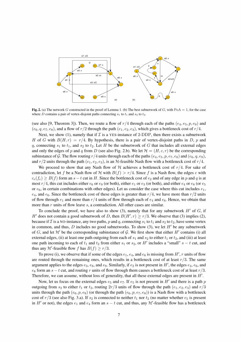
Fig. 2. (a) The network G constructed in the proof of Lemma 1. (b) The best subnetwork of G, with PoA = 1, for the casewhere D contains a pair of vertex-disjoint paths connecting s1 to t1 and s2 to t2.

(see also [9, Theorem 3]). Then, we route a flow of r/4 through each of the paths (e4, e5, p, e9) and(e6, q, e7, e8), and a flow of r/2 through the path (e1, e2, e3), which gives a bottleneck cost of r/4.

Next, we show (1), namely that if I is a YES-instance of 2-DDP, then there exists a subnetworkH of G with B(H, r) = r/4. By hypothesis, there is a pair of vertex-disjoint paths in D, p andq, connecting s1 to t1, and s2 to t2. Let H be the subnetwork of G that includes all external edgesand only the edges of p and q from D (see also Fig. 2.b). We let H = (H, c, r) be the correspondingsubinstance of G. The flow routing r/4 units through each of the paths (e4, e5, p, e7, e8) and (e6, q, e9),and r/2 units through the path (e1, e2, e3), is anH-feasible Nash flow with a bottleneck cost of r/4.

We proceed to show that any Nash flow of H achieves a bottleneck cost of r/4. For sake ofcontradiction, let f be a Nash flow of H with B(f) > r/4. Since f is a Nash flow, the edges e withce(fe) ≥ B(f) form an s− t cut in H . Since the bottleneck cost of e2 and of any edge in p and q is atmost r/4, this cut includes either e6 or e9 (or both), either e1 or e3 (or both), and either e4 or e8 (or e5

or e6, in certain combinations with other edges). Let us consider the case where this cut includes e1,e4, and e6. Since the bottleneck cost of these edges is greater than r/4, we have more than r/2 unitsof flow through e1 and more than r/4 units of flow through each of e4 and e6. Hence, we obtain thatmore than r units of flow leave s, a contradiction. All other cases are similar.

To conclude the proof, we have also to show (3), namely that for any subnetwork H ′ of G, ifH ′ does not contain a good subnetwork of D, then B(H ′, r) ≥ r/3. We observe that (3) implies (2),because if I is a NO-instance, any two paths, p and q, connecting s1 to t1 and s2 to t2, have some vertexin common, and thus, D includes no good subnetworks. To show (3), we let H ′ be any subnetworkof G, and let H′ be the corresponding subinstance of G. We first show that either H ′ contains (i) allexternal edges, (ii) at least one path outgoing from each of s1 and s2 to either t1 or t2, and (iii) at leastone path incoming to each of t1 and t2 from either s1 or s2, or H ′ includes a “small” s − t cut, andthus anyH′-feasible flow f has B(f) ≥ r/3.

To prove (i), we observe that if some of the edges e1, e4, and e6 is missing fromH ′, r units of floware routed through the remaining ones, which results in a bottleneck cost of at least r/3. The sameargument applies to the edges e3, e8, and e9. Similarly, if e2 is not present in H ′, the edges e4, e6, ande8 form an s− t cut, and routing r units of flow through them causes a bottleneck cost of at least r/3.Therefore, we can assume, without loss of generality, that all these external edges are present in H ′.

Now, let us focus on the external edges e5 and e7. If e5 is not present in H ′ and there is a path poutgoing from s2 to either t1 or t2, routing 2r/3 units of flow through the path (e1, e2, e3) and r/3units through the path (e6, p, e9) (or through the path (e6, p, e7, e8)) is a Nash flow with a bottleneckcost of r/3 (see also Fig. 3.a). If s2 is connected to neither t1 nor t2 (no matter whether e5 is presentin H ′ or not), the edges e1 and e4 form an s − t cut, and thus, any H′-feasible flow has a bottleneck

7

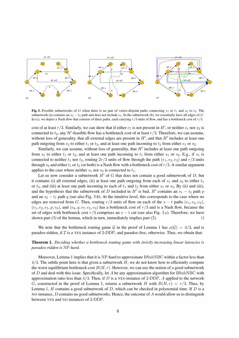
Fig. 3. Possible subnetworks of G when there is no pair of vertex-disjoint paths connecting s1 to t1 and s2 to t2. Thesubnetwork (a) contains an s2 − t2 path and does not include e5. In the subnetwork (b), we essentially have all edges of G.In (c), we depict a Nash flow that consists of three paths, each carrying r/3 units of flow, and has a bottleneck cost of r/3.

cost of at least r/3. Similarly, we can show that if either e7 is not present in H ′, or neither s1 nor s2 isconnected to t2, anyH′-feasible flow has a bottleneck cost of at least r/3. Therefore, we can assume,without loss of generality, that all external edges are present in H ′, and that H ′ includes at least onepath outgoing from s2 to either t1 or t2, and at least one path incoming to t2 from either s1 or s2.

Similarly, we can assume, without loss of generality, that H ′ includes at least one path outgoingfrom s1 to either t1 or t2, and at least one path incoming to t1 from either s1 or s2. E.g., if s1 isconnected to neither t1 nor t2, routing 2r/3 units of flow through the path (e1, e2, e3) and r/3 unitsthrough s2 and either t1 or t2 (or both) is a Nash flow with a bottleneck cost of r/3. A similar argumentapplies to the case where neither s1 nor s2 is connected to t1.

Let us now consider a subnetwork H ′ of G that does not contain a good subnetwork of D, butit contains (i) all external edges, (ii) at least one path outgoing from each of s1 and s2 to either t1or t2, and (iii) at least one path incoming to each of t1 and t2 from either s1 or s2. By (ii) and (iii),and the hypothesis that the subnetwork of D included in H ′ is bad, H ′ contains an s1 − t2 path pand an s2 − t1 path q (see also Fig. 3.b). At the intuitive level, this corresponds to the case where noedges are removed from G. Then, routing r/3 units of flow on each of the s − t paths (e1, e2, e3),(e1, e2, e5, p, e9), and (e6, q, e7, e2, e3) has a bottleneck cost of r/3 and is a Nash flow, because theset of edges with bottleneck cost r/3 comprises an s − t cut (see also Fig. 3.c). Therefore, we haveshown part (3) of the lemma, which in turn, immediately implies part (2). ut

We note that the bottleneck routing game G in the proof of Lemma 1 has ρ(G) = 4/3, and isparadox-ridden, if I is a YES instance of 2-DDP, and paradox-free, otherwise. Thus, we obtain that:

Theorem 1. Deciding whether a bottleneck routing game with strictly increasing linear latencies isparadox-ridden is NP-hard.

Moreover, Lemma 1 implies that it is NP-hard to approximate BSubNBC within a factor less than4/3. The subtle point here is that given a subnetwork H , we do not know how to efficiently computethe worst equilibrium bottleneck cost B(H, r). However, we can use the notion of a good subnetworkof D and deal with this issue. Specifically, let A be any approximation algorithm for BSubNBC withapproximation ratio less than 4/3. Then, if D is a YES-instance of 2-DDP, A applied to the networkG, constructed in the proof of Lemma 1, returns a subnetwork H with B(H, r) < r/3. Thus, byLemma 1, H contains a good subnetwork of D, which can be checked in polynomial time. If D is aNO-instance,D contains no good subnetworks. Hence, the outcome ofAwould allow us to distinguishbetween YES and NO instances of 2-DDP.

8

5 Approximating the Best Subnetwork is Hard

Next, we apply essentially the same construction as in the proof of Lemma 1, but in a recursive way,and show that it is NP-hard to approximate BSubNBC for linear bottleneck routing games within afactor of O(n.121−ε), for any constant ε > 0. Throughout this section, we let I = (D, s1, s2, t1, t2)be a 2-DDP instance, and let G be an s − t network, which includes (possibly many copies of) Dand can be constructed from I in polynomial time. We assume that G has a linear latency functionce(x) = aex, ae > 0, on each edge e, and for any traffic rate r > 0, the bottleneck routing gameG = (G, c, r) has B∗(G) = r/γ1, for some γ1 > 0. Moreover,

1. If I is a YES-instance of 2-DDP, there exists a subnetwork H of G with B(H, r) = r/γ1.2. If I is a NO-instance of 2-DDP, for all subnetworksH ′ ofG,B(H ′, r) ≥ r/γ2, for a γ2 ∈ (0, γ1).3. For all subnetworks H ′ of G, either H ′ contains at least one copy of a good subnetwork of D, orB(H ′, r) ≥ r/γ2.

The existence of such a network shows that it is NP-hard to approximate BSubNBC within a factorless than γ = γ1/γ2. Thus, we usually refer to G as a γ-gap instance (with linear latencies). Forexample, for the network G in the proof of Lemma 1, γ1 = 4 and γ2 = 3, and thus G is a 4/3-gapinstance. We next show that given I and a γ1/γ2-gap instance G, we can construct a 4γ1/(3γ2)-gapinstance G′, i.e., we can amplify the inapproximability gap by a factor of 4/3.

Lemma 2. Let I = (D, s1, s2, t1, t2) be a 2-DDP instance, and let G be a γ1/γ2-gap instance withlinear latencies, based on I. Then, we can construct, in time polynomial in the size of I and G, ans− t network G′ with a linear latency function ce(x) = aex, ae > 0, on each edge e, so that for anytraffic rate r > 0, the bottleneck routing game G′ = (G′, c, r) has B∗(G) = r/(4γ1), and:

1. If I is a YES-instance of 2-DDP, there exists a subnetwork H of G′ with B(H, r) = r/(4γ1).2. If I is a NO-instance of 2-DDP, for every subnetwork H ′ of G′, B(H ′, r) ≥ r/(3γ2).3. For all subnetworks H ′ of G′, either H ′ contains at least one copy of a good subnetwork of D, orB(H ′, r) ≥ r/(3γ2).

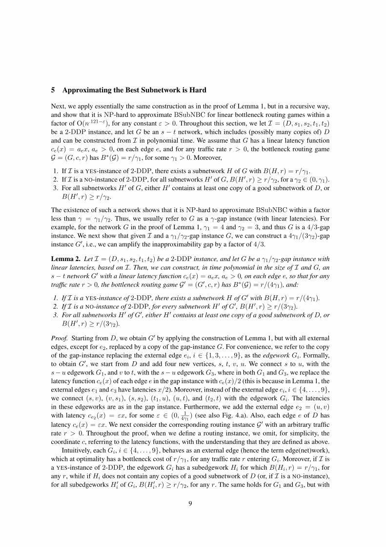
Proof. Starting from D, we obtain G′ by applying the construction of Lemma 1, but with all externaledges, except for e2, replaced by a copy of the gap-instance G. For convenience, we refer to the copyof the gap-instance replacing the external edge ei, i ∈ 1, 3, . . . , 9, as the edgework Gi. Formally,to obtain G′, we start from D and add four new vertices, s, t, v, u. We connect s to u, with thes−u edgework G1, and v to t, with the s−u edgework G3, where in both G1 and G3, we replace thelatency function ce(x) of each edge e in the gap instance with ce(x)/2 (this is because in Lemma 1, theexternal edges e1 and e3 have latencies x/2). Moreover, instead of the external edge ei, i ∈ 4, . . . , 9,we connect (s, v), (v, s1), (s, s2), (t1, u), (u, t), and (t2, t) with the edgework Gi. The latenciesin these edgeworks are as in the gap instance. Furthermore, we add the external edge e2 = (u, v)with latency ce2(x) = εx, for some ε ∈ (0, 1

4γ1) (see also Fig. 4.a). Also, each edge e of D has

latency ce(x) = εx. We next consider the corresponding routing instance G′ with an arbitrary trafficrate r > 0. Throughout the proof, when we define a routing instance, we omit, for simplicity, thecoordinate c, referring to the latency functions, with the understanding that they are defined as above.

Intuitively, each Gi, i ∈ 4, . . . , 9, behaves as an external edge (hence the term edge(net)work),which at optimality has a bottleneck cost of r/γ1, for any traffic rate r entering Gi. Moreover, if I isa YES-instance of 2-DDP, the edgework Gi has a subedgework Hi for which B(Hi, r) = r/γ1, forany r, while if Hi does not contain any copies of a good subnetwork of D (or, if I is a NO-instance),for all subedgeworks H ′i of Gi, B(H ′i, r) ≥ r/γ2, for any r. The same holds for G1 and G3, but with

9

Fig. 4. (a) The network G′ constructed in the proof of Lemma 2. The structure of G′ is similar to the structure of the networkG in Fig. 2, with each external edge ei, except for e2, replaced by the edgework Gi. (b) The structure of a best subnetworkH of G′, with PoA = 1, when D contains a pair of vertex-disjoint paths, p and q, connecting s1 to t1 and s2 to t2. Tocomplete H , we use an optimal subnetwork (or simply, subedgework) of each edgework Gi.

a worst equilibrium bottleneck cost of r/(2γ1) in the former case, and of r/(2γ2) in the latter case,because the latency functions of G1 and G3 are scaled by 1/2 (see also Proposition 1).

The proofs of the following propositions are conceptually similar to the proofs of the correspond-ing claims in the proof Lemma 1, and can be found in the Appendix, Sections A.3 and A.4.

Proposition 4. The optimal bottleneck cost of G′ is B∗(G′) = r/(4γ1).

Proposition 5. If I is a YES-instance, there is a subnetwork H of G′ with B(H, r) = r/(4γ1).

The most technical part of the proof is to show (3), namely that for any subnetworkH ′ ofG′, ifH ′

does not contain any copies of a good subnetwork of D, then B(H ′, r) ≥ r/(3γ2). This immediatelyimplies (2), since if I is a NO-instance of 2-DDP, D includes no good subnetworks. To prove (3),we consider any subnetwork H ′ of G′, and let H ′i be the subedgework of each Gi present in H ′. Weassume that the subedgeworksH ′i do not contain any copies of a good subnetwork ofD, and show thatif the subnetwork of D connecting s1 and s2 to t1 and t2 in H ′ is also bad, then B(H ′, r) ≥ r/(3γ2).

At the technical level, we repeatedly use the idea of a flow fi through a subedgework H ′i that “sat-urates”H ′i, in the sense that fi is a Nash flow with bottleneck cost at least ri/(3γ2) for the subinstance(H ′i, ri). Formally, we say that a flow rate ri saturates a subedgework H ′i if B(H ′i, ri) ≥ ri/(3γ2).We refer to the flow rate rsi for which B(H ′i, r

si ) = rsi /(3γ2) as the saturation rate of H ′i. We note

that the saturation rate rsi is well-defined, because the latency functions of Gis are linear and strictlyincreasing. Moreover, by property (3) of gap instances, the saturation rate of each subedgework H ′i isrsi ≤ r/3, if i ∈ 4, . . . , 9, and rsi ≤ 2r/3, if i ∈ 1, 3. Thus, at the intuitive level, the subedge-works H ′i behave as the external edges of the network constructed in the proof of Lemma 1. Hence,to show that B(H ′, r) ≥ r/(3γ2), we need to construct a flow of rate (at most) r that saturates acollection of subedgeworks comprising an s− t cut in H ′.

Our first step in this direction is to simplify the possible structure ofH ′. The proof of the followingproposition can be found in the Appendix, Section A.5.

Proposition 6. Let H ′ be any subnetwork of G′ whose subedgeworks H ′i do not contain any copiesof a good subnetwork of D. Then, either the subnetwork H ′ contains (i) the external edge e2, (ii) atleast one path outgoing from each of s1 and s2 to either t1 or t2, and (iii) at least one path incomingto each of t1 and t2 from either s1 or s2, or B(H ′, r) ≥ r/(3γ2).

Now, let us focus on a subnetwork H ′ of G′ that contains (i) the external edge e2, (ii) at least onepath outgoing from each of s1 and s2 to either t1 or t2, and (iii) at least one path incoming to each of

10

t1 and t2 from either s1 or s2. If the copy of the subnetwork of D connecting s1 and s2 to t1 and t2 inH ′ is also bad, properties (ii) and (iii) imply that H ′ contains an s1 − t2 path p and an s2 − t1 pathq. In this case, the entire subnetwork H ′ essentially behaves as if it included all edges of G′. Then, arouting similar to that in Fig. 3.c gives a Nash flow with a bottleneck cost of r/(3γ2). This intuition isformalized by the following proposition, whose proof can be found in the Appendix, Section A.6.

Proposition 7. Let H ′ be any subnetwork of G′ that satisfies (i), (ii), and (iii) above, and does notcontain any copies of a good subnetwork of D. Then B(H ′, r) ≥ r/(3γ2).

Propositions 6 and 7 immediately imply part (3) of the lemma, which, in turn, implies part (2). utEach time we apply Lemma 2 to a γ-gap instance G, we obtain a 4γ/3-gap instance G′ with a

number of vertices of at most 8 times the vertices of G plus the number of vertices of D. Therefore,if we start with an instance I = (D, s1, s2, t1, t2) of 2-DDP, where D has k vertices, and applyLemma 1 once, and subsequently apply Lemma 2 for blog4/3 kc times, we obtain a k-gap instanceG′, where the network G′ has n = O(k8.23) vertices. Suppose now that there is a polynomial-timealgorithm A that approximates the best subnetwork of G′ within a factor of O(k1−ε) = O(n0.121−ε),for some small ε > 0. Then, if I is a YES-instance of 2-DDP, algorithm A, applied to G′, shouldreturn a best subnetwork H with at least one copy of a good subnetwork of D. Since H contains apolynomial number of copies of subnetworks of D, and we can check whether a subnetwork of D isgood in polynomial time, we can efficiently recognize I as a YES-instance of 2-DDP. On the otherhand, if I is a NO-instance of 2-DDP, D includes no good subnetworks. Again, we can efficientlycheck that in the subnetwork returned by algorithm A, there are not any copies of a good subnetworkof D, and hence recognize I as a NO-instance of 2-DDP. Thus, we obtain that:

Theorem 2. For bottleneck routing games with strictly increasing linear latencies, it is NP-hard toapproximate BSubNBC within a factor of O(n0.121−ε), for any constant ε > 0.

6 Networks with Quasipolynomially Many Paths

In this section, we approximate, in quasipolynomial-time, the best subnetwork and its worst equilib-rium bottleneck cost for instances G = (G, c, r) where the network G has quasipolynomially manys− t paths, the latency functions are continuous and satisfy a Lipschitz condition, and the worst Nashflow in the best subnetwork routes a non-negligible amount of flow on all used edges.

We highlight that the restriction to networks with quasipolynomially many s− t paths is somehownecessary, in the sense that Theorem 2 shows that if the network has exponentially many s− t paths,as it happens for the hard instances of 2-DDP, and thus for the networks G and G′ constructed in theproofs of Lemma 1 and Lemma 2, it is NP-hard to approximate BSubNBC within any reasonablefactor. Also, we can always assume, without loss of generality, that the worst Nash flow of the bestsubnetworkH∗ assigns positive flow to all edges ofH∗. Otherwise, we can remove any unused edges,without increasing the worst equilibrium bottleneck cost ofH∗. In addition, we assume here that thereis a constant δ > 0, such that the worst Nash flow in H∗ routes more than δ units of flow on all edgesof the best subnetwork H∗.

In the following, we normalize the traffic rate r to 1. This is for convenience and can be madewithout loss of generality5. Our algorithm is based on [10, Lemma 2], which applies Althofer’s “Spar-sification” Lemma [1], and shows that any flow can be approximated by a “sparse” flow using loga-rithmically many paths.

5 Given a bottleneck routing game G with traffic rate r > 0, we can replace each latency function ce(x) with ce(rx), andobtain a bottleneck routing game G′ with traffic rate 1, and the same Nash flows, PoA, and solutions to BSubNBC.

11

Lemma 3. Let G = (G(V,E), c, 1) be a routing instance, and let f be any G-feasible flow. Then, forany ε > 0, there exists a G-feasible flow f using at most k(ε) = blog(2m)/(2ε2)c + 1 paths, suchthat for all edges e, |fe − fe| ≤ ε, if fe > 0, and fe = 0, otherwise.

By Lemma 3, there exists a sparse flow f that approximates the worst Nash flow f on the bestsubnetwork H∗ of G. Moreover, the proof of [10, Lemma 2] shows that the flow f is determined bya multiset P of at most k(ε) paths, selected among the paths used by f . Then, for every path p ∈ P ,fp = |P (p)|/|P |, where |P (p)| is number of times the path p is included in the multiset P , and |P |is the cardinality of P . Therefore, if the total number |P| of s − t paths in G is quasipolynomial, wecan find, in quasipolynomial-time, by exhaustive search, a flow-subnetwork pair that approximates theoptimal solution of BSubNBC. Based on this intuition, we next obtain an approximation algorithmfor BSubNBC on networks with quasipolynomially many paths, under the assumption that there is aconstant δ > 0, such that the worst Nash flow in the best subnetwork H∗ routes more than δ units offlow on all edges of H∗. This assumption is necessary so that the exhaustive search on the family ofsparse flows of Lemma 3 can generate the best subnetwork H∗, which is crucial for the analysis.

Theorem 3. Let G = (G(V,E), c, 1) be a bottleneck routing game with continuous latency functionsthat satisfy the Lipschitz condition with a constant ξ > 0, let H∗ be the best subnetwork of G, andlet f∗ be the worst Nash flow in H∗. If for all edges e of H∗, f∗e > δ, for some constant δ > 0,then for any constant ε > 0, we can compute in time |P|O(log(2m)/minδ2,ε2/ξ2) a flow f and asubnetwork H such that: (i) f is an ε/2-Nash flow in the subnetwork H , (ii) B(f) ≤ B(H∗, 1) + ε,(iii) B(H, 1) ≤ B(f) + ε/4, and (iv) B(f) ≤ B(H, 1) + ε/2.

Proof. Let ε > 0 be a constant, and let ε1 = minδ, ε/(4ξ), and ε2 = ε/2. We show that aflow-subnetwork pair (H, f) with the desired properties can be computed in time |P|O(k(ε1)), wherek(ε1) = blog(2m)/min2δ2, ε2/(8ξ2)c + 1, For convenience, we say that a flow g is a candidateflow if there is a multiset P of paths from P , with |P | ≤ k(ε1), such that gp = |P (p)|/|P |, for eachp ∈ P . Namely, a candidate flow belongs to the family of sparse flows, which by Lemma 3, can ap-proximate any other flow. Similarly, a subnetwork H is a candidate subnetwork if there is a candidateflow g such that H consists of the edges used by g (and only of them), and a subnetwork-flow pair(H, g) is a candidate solution, if g is a candidate flow, H is a candidate subnetwork that includes allthe edges used by g (and possibly some other edges), and g is an ε2-Nash flow in H .

By exhaustive search, in time |P|O(k(ε1)), we generate all candidate flows, all candidate subnet-works, and compute the bottleneck cost B(g) of any candidate flow g. Then, for each pair (H, g),where g is a candidate flow and H is a candidate subnetwork, we check, in polynomial time, whetherg is an ε2-Nash flow in H , and thus whether (H, g) is a candidate solution. Thus, in time |P|O(k(ε1)),we determine all candidate solutions. For each candidate subnetwork H that participates in at leastone candidate solution, we let B(H) be the maximum bottleneck cost B(g) of a candidate flow g forwhich (H, g) is a candidate solution. The algorithm returns the subnetwork H that minimizes B(H),and a flow f for which (H, f) is a candidate solution and B(H) = B(f).

The exhaustive search above can be implemented in |P|O(k(ε1)) time. As for the properties of thesolution (H, f), the definition of candidate solutions immediately implies (i), i.e., that f is an ε/2-Nash flow in H . In the Appendix, Section A.7, we use Lemma 3, and show (ii), (iii), and (iv). ut

Therefore, the algorithm of Theorem 3 returns a flow-subnetwork pair (H, f) such that f is anε/2-Nash flow in H , the worst equilibrium bottleneck cost of the subnetwork H approximates theworst equilibrium bottleneck cost of H∗, since B(H∗, 1) ≤ B(H, 1) ≤ B(H∗, 1) + 5ε/4, by (ii)and (iii), and the bottleneck cost of f approximates the worst equilibrium bottleneck cost of H , sinceB(H, 1)− ε/4 ≤ B(f) ≤ B(H, 1) + ε/2, by (iii) and (iv).

12

References

1. I. Althofer. On sparse approximations to randomized strategies and convex combinations. Linear Algebra and Appli-cations, 99:339-355, 1994.

2. Y. Azar and A. Epstein. The hardness of network design for unsplittable flow with selfish users. In Proc. of the 3rdWorkshop on Approximation and Online Algorithms (WAOA ’05), LNCS 3879, pp. 41-54, 2005.

3. R. Banner and A. Orda. Bottleneck routing games in communication networks. IEEE Journal on Selected Areas inCommunications, 25(6):1173-1179, 2007.

4. D. Braess. Uber ein paradox aus der Verkehrsplanung. Unternehmensforschung, 12:258-268, 1968.5. C. Busch and M. Magdon-Ismail. Atomic routing games on maximum congestion. Theoretical Computer Science,

410:3337-3347, 2009.6. I. Caragiannis, C. Galdi, and C. Kaklamanis. Network load games. In Proc. of the 16th Symp. on Algorithms and

Computation (ISAAC ’05), LNCS 3827, pp. 809-818, 2005.7. R. Cole, Y. Dodis, and T. Roughgarden. Bottleneck links, variable demand, and the tragedy of the commons. In Proc.

of the 17th ACM-SIAM Symposium on Discrete Algorithms (SODA ’06), pp. 668-677, 2006.8. A. Epstein, M. Feldman, and Y. Mansour. Efficient graph topologies in network routing games. Games and Economic

Behaviour, 66(1):115125, 2009.9. S. Fortune, J.E. Hopcroft, and J. Wyllie. The directed subgraph homeomorphism problem. Theoretical Computer

Science, 10:111-121, 1980.10. D. Fotakis, A.C. Kaporis, and P.G. Spirakis. Efficient methods for selfish network design. In Proc. of the 36th Collo-

quium on Automata, Languages and Programming (ICALP-C ’09), LNCS 5556, pp. 459-471, 2009.11. H. Hou and G. Zhang. The hardness of selective network design for bottleneck routing games. In Proc. of the 4th

Conference on Theory and Applications of Models of Computation (TAMC ’07), LNCS 4484, pp. 58-66, 2007.12. E. Koutsoupias and C. Papadimitriou. Worst-case equilibria. In Proc. of the 16th Symposium on Theoretical Aspects of

Computer Science (STACS ’99), LNCS 1563, pp. 404-413, 1999.13. H. Lin, T. Roughgarden, and E. Tardos. A stronger bound on Braess’s paradox. In Proc. of the 15th ACM-SIAM

Symposium on Discrete Algorithms (SODA ’04), pp. 340-341, 2004.14. H. Lin, T. Roughgarden, E. Tardos, and A. Walkover. Braess’s paradox, Fibonacci numbers, and exponential inapprox-

imability. In Proc. of the 32th Colloquium on Automata, Languages and Programming (ICALP ’05), LNCS 3580, pp.497-512, 2005.

15. V. Mazalov, B. Monien, F. Schoppmann, and K. Tiemann. Wardrop equilibria and price of stability for bottleneck gameswith splittable traffic. In Proc. of the 2nd Workshop on Internet and Network Economics (WINE ’06), LNCS 4286, pp.331-342, 2006.

16. I. Milchtaich. Network topology and the efficiency of equilibrium. Games and Economic Behavior, 57:321346, 2006.17. T. Roughgarden. On the severity of Braess’s paradox: Designing networks for selfish users is hard. Journal of Computer

and System Sciences, 72(5):922-953, 2006.

A Appendix

A.1 The Proof of Proposition 1

Since the traffic rate of both G and G′ is r, any G-feasible flow f is also G′-feasible. Moreover, theG′-latency of f on each edge e is αce(fe). This immediately implies that BG′(f) = αBG(f), and thatf is a Nash flow (resp. optimal flow) of G iff f is a Nash flow (resp. optimal flow) of G′. ut

A.2 The Proof of Proposition 1

Let f be any Nash flow of G. We use induction on the series-parallel structure of the network G, andshow that f is an optimal flow w.r.t the bottleneck cost, i.e., that B(f) = B∗(G). For the basis, weobserve that the claim holds if G consists of a single edge (s, t). For the inductive step, we distinguishtwo cases, depending on whether G is obtained by the series or the parallel composition of two series-parallel networks G1 and G2.Series Composition. First, we consider the case where G is obtained by the series composition of ans− t′ series-parallel network G1 and a t′− t series-parallel network G2. We let f1 and f2, both of rater, be the restrictions of f into G1 and G2, respectively.

13

We start with the case where B(f) = B(f1) = B(f2). Then, either f1 is a Nash flow in G1,or f2 is a Nash flow in G2. Otherwise, there would be an s − t′ path p1 in G1 with bottleneck costbp1(f1) < B(f1), and an t′ − t path p2 in G2, with bottleneck cost bp2(f2) < B(f2). Combiningp1 and p2, we obtain an s − t path p = p1 ∪ p2 in G with bottleneck cost smaller than B(f), whichcontradicts the hypothesis that f is a Nash flow of G. If f1 (or f2) is a Nash flow inG1 (resp.G2), thenby induction hypothesis f1 (resp. f2) is an optimal flow in G1 (resp. in G2), and thus f is an optimalflow of G.

Otherwise, we assume, without loss of generality, thatB(f) = B(f1) < B(f2). Then, f1 is a Nashflow in G1. Otherwise, there would be an s− t′ path p1 in G1 with bottleneck cost bp1(f1) < B(f1),which could be combined with any t′ − t path p2 in G2, with bottleneck cost B(f2) < B(f1), intoan s − t path p = p1 ∪ p2 with bottleneck cost smaller than B(f). The existence of such a path pcontradicts the the hypothesis that f is a Nash flow of G. Therefore, by induction hypothesis f1 is anoptimal flow in G1, and thus f is an optimal flow of G.

Parallel Composition. Next, we consider the case where G is obtained by the parallel compositionof an s− t series-parallel network G1 and an s− t series-parallel network G2. We let f1 and f2 be therestriction of f into G1 and G2, respectively, let r1 (resp. r2) be the rate of f1 (resp. f2), and let G1

(resp. G2) be the corresponding routing instance. Then, since f is a Nash flow of G, f1 and f2 are Nashflows of G1 and G2 respectively, andB(f1) = B(f2) = B(f). Therefore, by the induction hypothesis,f1 and f2 are optimal flows of G1 and G2, and f is an optimal flow of G. To see this, we observe thatany flow different from f must route more flow through either G1 or G2. But if the flow through e.g.G1 is more than r1, the bottleneck cost through G1 would be at least as large as B(f1). ut

A.3 The Proof of Proposition 4

We have to show thatB∗(G′) = r/(4γ1). For the upper bound, as in the proof of Lemma 1, we assumethat D contains an s1 − t2 path p and an s2 − t1 path q, which are edge-disjoint. We route (i) r/4units of flow through the edgeworks G4, G5, next through the path p, and next through the edgeworkG9, (ii) r/4 units through the edgeworks G6, next through the path q, and next through the edgeworksG7 and G8, and (ii) r/2 units through the edgework G1, next through the external edge e2, and nextthrough the edgework G3. These routes are edge(work)-disjoint, and if we route the flow optimallythrough each edgework, the bottleneck cost is r/(4γ1). As for the lower bound, we observe that theedgeworks H1, H4, and H6 essentially form an s − t cut in G′, and thus every feasible flow has abottleneck cost of at least r/(4γ1). ut

A.4 The Proof of Proposition 5

If I is a YES-instance of 2-DDP, then (i) there are two vertex-disjoint paths in D, p and q, connectings1 to t1 and s2 to t2, and (ii) there is an optimal subnetwork (or simply, subedgework) Hi of eachedgework Gi so that for any traffic rate r routed through Hi, the worst equilibrium bottleneck costB(Hi, r) is r/γ1, if i ∈ 4, . . . , 9, and r/(2γ1), if i ∈ 1, 3. Let H be the subnetwork of G′ thatconsists of only the edges of the paths p and q from D, of the external edge e2, and of the optimalsubedgeworks Hi, i ∈ 1, 3, . . . , 9 (see also Fig. 4.b). We observe that we can route: (i) r/4 units offlow through the subedgeworks H4, H5, next through the path p, and next through the subedgeworksH7 and H8, (ii) r/4 units of flow through the subedgework H6, next through the path q, and nextthrough the subedgework H9, and (iii) r/2 units of flow through the subedgework H1, next throughthe external edge e2, and next through the subedgeworkH3. These routes are edge(work)-disjoint, and

14

if we use any Nash flow through each of the routing instances (Hi, r/4), i ∈ 4, . . . , 9, (H1, r/2),and (H3, r/2), we obtain a Nash flow of the instance (H, r) with a bottleneck cost of r/(4γ1).

We next show that any Nash flow of (H, r) has a bottleneck cost of at most r/(4γ1). To reacha contradiction, let us assume that some feasible Nash flow f has bottleneck cost B(f) > r/(4γ1).We recall that f is a Nash flow iff the edges of G′ with bottleneck cost B(f) > r/(4γ1) form ans − t cut. This cut does not include the edges of the paths p and q and the external edge e2, due tothe choice of their latencies. Hence, this cut includes a similar cut either in H6 or in H9 (or in both),either in H1 or H3 (or in both), and either in H4 or in H8 (or in H5 or in H6, in certain combinationswith other subedgeworks, see also Fig. 4.b). Let us consider the case where the edges with bottleneckcost B(f) > r/(4γ1) form a cut in H1, H4, and H6. Namely, the edges of H1, H4, and H6, withbottleneck cost equal to B(f) > r/(4γ1) form an s− u, an s− v, and an s− s2 cut, respectively, andthus the restriction of f to each of H1, H4, and H6, is an equilibrium flow of bottleneck cost greaterthan r/(4γ1) for the corresponding routing instance. Since I is a YES-instance, this can happen onlyif the flow through H1 is more than r/2, and the flow through each of H4 and H6 is more than r/4(see also property (ii) of optimal subedgeworks above). Hence, we obtain that more than r units offlow leave s, a contradiction. All other cases are similar. ut

A.5 The Proof of Proposition 6

For convenience, in the proofs of Proposition 6 and Proposition 7, we slightly abuse the terminology,and say that a collection of subedgeworks of H ′ form an s − t cut, if the union of any cuts in themcomprises an s − t cut in H ′. Moreover, whenever we write that ri units of flow are routed througha subedgework Hi, we assume that the routing through Hi corresponds to the worst Nash flow of(Hi, ri). Also, we recall that since subedgeworks H ′i do not contain any copies of a good subnetworkof D, by property (3) of gap instances, the saturation rate of each H ′i is rsi ≤ r/3, if i ∈ 4, . . . , 9,and rsi ≤ 2r/3, if i ∈ 1, 3.

We start by showing that either the external edge e2 is present in H ′, or B(H ′, r) ≥ r/(3γ2).Indeed, if e2 is not present inH ′, the subedgeworksH ′4,H ′6, andH ′8 form an s−t cut inH ′. Therefore,we can construct a Nash flow f that routes at least r/3 units of flow through H ′4, H ′6, and H ′8, and hasB(f) ≥ r/(3γ2). Therefore, we can assume, without loss of generality, that e2 is present in H ′.

Similarly, we show that either H ′ includes at least one path outgoing from s2 to either t1 or t2,and at least one path incoming to t2 from either s1 or s2, or B(H ′, r) ≥ r/(3γ2). In particular, if s2

is connected to neither t1 nor t2, the subedgeworks H ′1 and H ′4 form an s − t cut in H ′. Thus, wecan construct a Nash flow f that saturates the subedgework H ′1 (or the subedgeworks H ′3 and H ′8,if rs1 > rs3 + rs8) and the subedgework H ′4 (or the subedgeworks H ′3 and either H ′5, or H ′9 and atleast one of the H ′7 and H ′8, depending on rs4 and the saturation rates of the rest). We note that thisis always possible with r units of flow, because rs1 ≤ 2r/3 and rs4 ≤ r/3. Therefore, the bottleneckcost of f is B(f) ≥ r/(3γ2). In case where there is no path incoming to t2 from either s1 or s2,the subedgeworks H ′3 and H ′8 form an s − t cut in H ′. As before, we can construct a Nash flowf that saturates the subedgeworks H ′3 and H ′8 (or, as before, an appropriate combination of othersubedgeworks carrying flow to H ′3 and H ′8), and has B(f) ≥ r/(3γ2). Therefore, we can assume,without loss of generality, that H ′ includes at least one path outgoing from s2 to either t1 or t2, and atleast one path incoming to t2 from either s1 or s2.

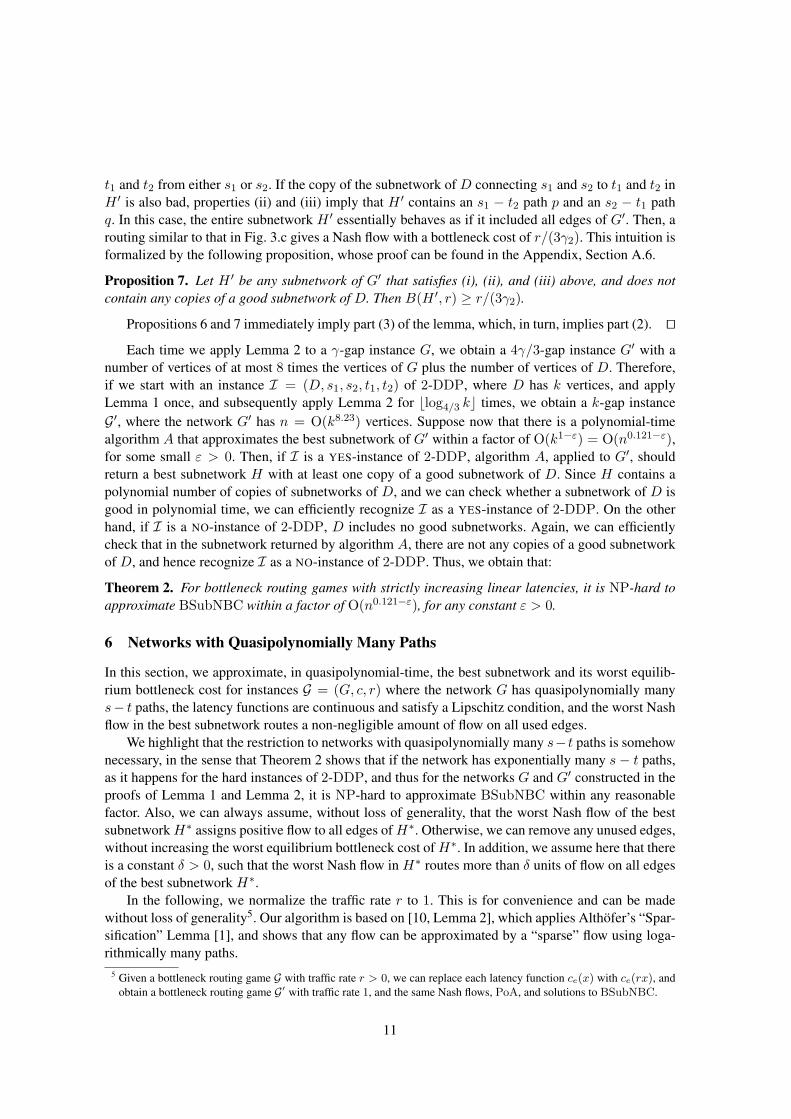
Next, we show that either H ′ includes at least one path outgoing from s1 to either t1 or t2, andat least one path incoming to t1 from either s1 or s2, or B(H ′, r) ≥ r/(3γ2). In particular, let usconsider the case where s1 is connected to neither t1 nor t2 (see also Fig. 5.a, the case where there isno path incoming to t1 from either s1 or s2 can be handled similarly). In the following, we assume

15

Fig. 5. The structure of possible subnetworks of G′ when there is no pair of vertex-disjoint paths connecting s1 to t1 ands2 to t2. The subnetwork (a) contains a path outgoing from s2 to either t1 or t2, and no path outgoing from s1 to either t1or t2. Hence, no flow can be routed through the edgework G5, and thus we can regard G5 as being absent from H ′. Thesubnetwork (b) essentially corresponds to the case where all edges of G′ are present in H ′.

that s2 is connected to t2 (because, by the analysis above, we can assume that there is a path incomingto t2, and s1 is not connected to T2), and construct a Nash flow f of bottleneck cost B(f) ≥ r/(3γ2).

We first route minrs6, rs9 ≤ r/3 units of flow through the subedgework H ′6, next through ans2− t2 path, and finally through the subedgework H ′9, and saturate either H ′6 or H ′9 (or both). If thereis an s2 − t1 path and H ′6 is not saturated, we keep routing flow through H ′6, next through an s2 − t1path, and next through the subedgeworks H ′7 and H ′8, until either the subedgework H ′6 or at least oneof the subedgeworks H ′7 and H ′8 become saturated. Thus, we saturate at least one edgework on everys− t path that includes s2.

Next, we show how to saturate at least one edgework on every s− t path that includes either v oru. If rs1 ≤ rs3 ≤ 2r/3, we route rs1 units of flow through H ′1, e2, and H ′3, and route minrs3 − rs1, rs4units of flow through H ′4 and H ′3, and saturate either H ′1 and H ′3 or H ′1 and H ′4. If rs3 < rs1 ≤ 2r/3,we route rs3 units of flow through H ′1, e2, and H ′3, and route minrs3 − rs1, rs8 units of flow throughH ′1 and H ′8, and saturate either H ′1 and H ′3 or H ′3 and H ′8.

The remaining flow (if any) can be routed through these routes, in proportional rates. In all cases,we obtain an s− t cut consisting of saturated subedgeworks. Thus, the resulting flow f is a Nash flowwith a bottleneck cost of at least r/(3γ2). ut

A.6 The Proof of Proposition 7

In the following, we consider a subnetwork H ′ of G′ which does not include any copies of a goodsubnetwork of D, and contains (i) the external edge e2, (ii) at least one path outgoing from eachof s1 and s2 to either t1 or t2, and (iii) at least one path incoming to each of t1 and t2 from eithers1 or s2. Since the copy of the subnetwork of D connecting s1 and s2 to t1 and t2 in H ′ is bad,properties (ii) and (iii) imply that H ′ contains an s1− t2 path p and an s2− t1 path q. Moreover, sincethe subedgeworks H ′i do not include any copies of a good subnetwork of D, by property (3) of gapinstances, the saturation rate of each H ′i is rsi ≤ r/3, if i ∈ 4, . . . , 9, and rsi ≤ 2r/3, if i ∈ 1, 3.

We next show that for such a subnetwork H ′, we can construct a Nash flow f of bottleneck costB(f) ≥ r/(3γ2). At the conceptual level, as in the last case in the proof of Lemma 1, we seek toconstruct a Nash flow by routing r/3 units of flow through each of the following three routes: (i) H ′1,e2, and H ′3, (ii) H ′1, e2, H ′5, p, and H ′9, and (iii) H ′6, q, H ′7, e2, and H ′3. However, for simplicity of theanalysis, we regard the corresponding (edge) flow as being routed through just two routes: a rate of2r/3 is routed through H ′1, e2, and H ′3, and a rate of r/3 is routed through the (possibly non-simple)route H ′6, q, H ′7, e2, H ′5, p, and H ′9. We do so because the latter routing allows us to consider fewer

16

cases in the analysis. We conclude the proof by showing that if the latter route is not simple, we canalways decompose the flow into the three simple routes above.

In the following, we assume that with a flow rate of at most 2r/3, routed through H ′1, e2, and H ′3(and possibly through H ′4 and H ′8), we can saturate both subedgeworks H ′1 and H ′3. Otherwise, as inthe last case in the proof of Proposition 6, we can show how with a total flow rate of at most 2r/3,part of which is routed through either H ′4 or H ′8, we can saturate either H ′1 and H ′4, or H ′3 and H ′8.Then, the remaining r/3 units of flow can saturate either H ′6, in the former case, or H ′9, in the lattercase. Thus, we obtain a Nash flow with a bottleneck cost of at least r/(3γ2).

Having saturated both subedgeworksH ′1 andH ′3, using at most 2r/3 units of flow, we have at leastr/3 units of flow to saturate the subedgeworks H ′5, H ′6, H ′7, and H ′9, or an appropriate subset of them,so that together withH ′1 andH ′3, they form an s−t cut inH ′. We first route τ ≡ minrs5, rs6, rs7, rs9 ≤r/3 units of flow throughH ′6, q,H ′7, e2,H ′5, p, andH ′9, until t, and consider different cases, dependingon which of the subedgeworks H ′5, H ′6, H ′7, and H ′9 has the minimum saturation rate.

– If τ = rs9, H ′9 is saturated. We first assume that H ′ contains an s1 − t1 path, and route (some of)the remaining flow (i) through H ′4, H ′5, an s1 − t1 path, H ′7, and H ′8, and (ii) through H ′6, q, H ′7,andH ′8. We do so until either at least one of the subedgeworksH ′7 andH ′8 or the subedgeworkH ′6and at least one of the subedgeworksH ′4 andH ′5 become saturated. Since minrs7, rs8 ≤ r/3, thisrequires at most r/3−τ additional units of flow. IfH ′ does not contain an s1−t1 path, we route theremaining flow only through route (ii), until either at least one of the subedgeworks H ′7 and H ′8 orthe subedgeworkH ′6 become saturated. In both cases, the newly saturated subedgeworks, togetherwith the saturated subedgeworks H ′1, H ′3, and H ′9, form an s − t cut of saturated subedgeworks,and thus the worst equilibrium bottleneck cost is at least r/(3γ2).

– If τ = rs6, H ′6 is saturated. As before, we first assume that H ′ contains an s1 − t1 path, and routethe remaining flow (i) throughH ′4,H ′5, p, andH ′9, and (ii) throughH ′4,H ′5, an s1−t1 path,H ′9 andH ′8, until either at least one of the subedgeworks H ′4 and H ′5, or the subedgework H ′9 and at leastone of the subedgeworks H ′7 and H ′8 become saturated. Since minrs4, rs5 ≤ r/3, this requiresat most r/3 − τ additional units of flow. If H ′ does not contain an s1 − t1 path, we route theremaining flow only through route (i), until either at least one of the subedgeworks H ′4 and H ′5 orthe subedgeworkH ′9 become saturated. In both cases, the newly saturated subedgeworks, togetherwith the saturated subedgeworks H ′1, H ′3, and H ′6, form an s − t cut of saturated subedgeworks,and thus the worst equilibrium bottleneck cost is at least r/(3γ2).

– If τ = rs7, H ′7 is saturated. Then, we first assume that H ′ contains an s2 − t2 path, and route theremaining flow (i) through H ′4, H ′5, p, and H ′9, and (ii) through H ′6, an s2 − t2 path, and H ′9, untileither the subedgework H ′9, or the subedgework H ′6 and at least one of the subedgeworks H ′4 andH ′5 become saturated. Since rs9 ≤ r/3, this requires at most r/3− τ additional units of flow. If H ′

does not contain an s2 − t2 path, we route the remaining flow only through route (i), until eitherat least one of the subedgeworks H ′4 and H ′5 or the subedgework H ′9 become saturated. In bothcases, the newly saturated subedgeworks, together with the saturated subedgeworks H ′1, H ′3, andH ′7, form an s − t cut of saturated subedgeworks, and thus the worst equilibrium bottleneck costis at least r/(3γ2).

– If τ = rs5, H ′5 is saturated. As before, we first assume that H ′ contains an s2 − t2 path, and routethe remaining flow (i) through H ′6, q, H ′7, and H ′8, and (ii) through H ′6, an s2 − t2 path, and H ′9,until either the subedgework H ′6, or the subedgework H ′9 and at least one of the subedgeworks H ′7and H ′8 become saturated. Since rs6 ≤ r/3, this requires at most r/3− τ additional units of flow.If H ′ does not contain an s2 − t2 path, we route the remaining flow only through route (i), untileither at least one of the subedgeworks H ′7 and H ′8 or the subedgework H ′6 become saturated. In

17

both cases, the newly saturated subedgeworks, together with the saturated subedgeworks H ′1, H ′3,and H ′5, form an s − t cut of saturated subedgeworks, and thus the worst equilibrium bottleneckcost is at least r/(3γ2).

Thus, in all cases, we obtain an equilibrium flow with a bottleneck cost of at least r/(3γ2). How-ever, in the construction above, the route H ′6, q, H ′7, e2, H ′5, p, H ′9 may not be simple, since p andq may not be vertex-disjoint. If this is the case, this route is technically not allowed by our model,where the flow is only routed through simple s − t paths. Nevertheless, the corresponding edge flowcan be decomposed into the following three simple routes: (i) H ′1, e2, and H ′3, (ii) H ′1, e2, H ′5, p, andH ′9, and (iii) H ′6, q, H ′7, e2, and H ′3, unless minrs1, rs3 ≤ r/3. Moreover, if minrs1, rs3 ≤ r/3, wecan work as above, and saturate both H ′1 and H ′3 with at most r/3 units of flow. The remaining 2r/3units of flow can be routed (i) through H ′6, q, H ′7, and H ′8, and (ii) through H ′4, H ′5, p, and H ′9, andpossibly either through H ′6, an s2− t2 path6, andH ′9, or through H ′4, H ′5, an s1− t1 path, H ′7, andH ′8,until either H ′4 (or H ′5) and H ′6, or H ′7 (or H ′8) and H ′9 are saturated. This routing only uses simpleroutes. In addition, these saturated subedgeworks, together with the saturated subedgeworks H ′1 andH ′3, form an s− t cut of saturated subedgeworks, and thus the worst equilibrium bottleneck cost is atleast r/(3γ2). ut

A.7 Theorem 3: The Proofs of (ii), (iii), and (iv)

We first show (ii), i.e., that B(f) ≤ B(H∗, 1) + ε. We recall that H∗ denotes the best subnetwork ofG and f∗ denotes the worst Nash flow in H∗. Also, by hypothesis, f∗e > δ > 0, for all edges e of H∗.

By Lemma 3, there is a candidate flow f such that for all edges e of H∗, |fe − f∗e | ≤ ε1. Thus,since ε1 ≤ δ, H∗ is a candidate network, because fe > 0 for all edges e of H∗. Moreover, by theLipschitz condition and the choice of ε1, for all edges e of H∗, |ce(fe) − ce(f∗e )| ≤ ε/4. Therefore,since f∗ is a Nash flow in H∗, f is an ε2-Nash flow in H∗, and thus (H, f) is a candidate solution.Furthermore, |B(f) − B(f∗)| ≤ ε/4, i.e., the bottleneck cost of f is within an additive term of ε/4from the worst equilibrium bottleneck cost of H∗. In particular, B(f) ≤ B(H∗, 1) + ε/4.

We also need to show that for any other candidate flow g for which (H∗, g) is a candidate solution,B(g) ≤ B(f)+3ε/4, and thus B(H∗) ≤ B(f)+3ε/4 ≤ B(H∗, 1)+ε. To reach a contradiction, letus assume that there is a candidate flow g that is an ε2-Nash flow inH∗ and hasB(g) > B(f)+3ε/4.But then, we should expect that there is a Nash flow g′ in H∗ that closely approximates g and has abottleneck cost of B(g′) ≈ B(g) > B(f∗), a contradiction. Formally, since g is an ε2-Nash flow inH∗, the set of edges with ce(ge) ≥ B(g)− ε/2 comprises an s− t cut in H∗. Then, by the continuityof the latency functions, we can fix a part of the flow routed essentially as in g, so that there is an s− tcut consisting of used edges with latency B(g)− ε/2, and possibly unused edges with latency at leastB(g)− ε/2, and reroute the remaining flow on top of it, so that we obtain a Nash flow g′ in H∗. Butthen,

B(g′) ≥ B(g)− ε/2 > B(f) + ε/4 ≥ B(f∗) ,

which contradicts the hypothesis that f∗ is the worst Nash flow in H∗.Therefore, B(H∗) ≤ B(H∗, 1)+ε. Since the algorithm returns the candidate solution (H, f), and

not a candidate solution including H∗, B(H) ≤ B(H∗). Thus, we obtain (ii), namely that B(H) =B(f) ≤ B(H∗, 1) + ε.

We proceed to show (iii), namely that B(H, 1) ≤ B(f) + ε/4. To this end, we let g be the worstNash flow inH . By Lemma 3, there is a candidate flow g such that for all edges e ofH , |ge−ge| ≤ ε1,

6 We note that if the paths p and q are not vertex-disjoint, we also have an s1 − t1 path and an s2 − t2 path in H ′.

18

if ge > 0, and ge = 0, otherwise. Therefore, by the Lipschitz condition and the choice of ε1, for alledges e of H , |ce(ge) − ce(ge)| ≤ ε/4, if ge > 0, and ce(ge) = ce(ge) = 0, otherwise. This impliesthat |B(g) − B(g)| ≤ ε/4, i.e., that bottleneck cost of g is within an additive term of ε/4 from thebottleneck cost of g. In particular, B(g) ≤ B(g) + ε/4.

We also need to show that (H, g) is a candidate solution. Since H is a candidate subnetwork andg is a candidate flow, we only need to show that g is an ε2-Nash flow in H . Since g is a Nash flowin H , the set of edges C = e : ce(ge) ≥ B(g) comprises an s − t cut in H . In fact, for all edgese ∈ C, ce(ge) = B(g), if ge > 0, and ce(ge) ≥ B(g), otherwise. Let us now consider the latency in gof each edge e ∈ C. If ge = 0, then ce(ge) = ce(ge) ≥ B(g) ≥ B(g)− ε/4. If ge > 0, then

B(g) ≥ ce(ge) ≥ ce(ge)− ε/4 = B(g)− ε/4 ≥ B(g)− ε/2 .

Therefore, for the flow g, we have an s − t cut in H consisting of edges e either with ge > 0 andB(g) − ε/2 ≤ ce(ge) ≤ B(g), or with ge = 0 and ce(ge) ≥ B(g) − ε/4. By the standard propertiesof ε-Nash flows (see also in Section 2), we obtain that g is a ε2-Nash flow in H .

Hence, we have shown that (H, g) is a candidate solution, and thatB(g) ≤ B(g)+ε/4. Therefore,the algorithm considers both candidate solutions (H, f) and (H, g), and returns (H, f), which impliesthat B(g) ≤ B(f). Thus, we obtain (iii), namely that B(H, 1) = B(g) ≤ B(f) + ε/4.

To conclude the proof, we next show (iv), namely that B(f) ≤ B(H, 1) + ε/2. For the proof,we use the same notation as in (iii). The argument is essentially identical to that used in the secondpart of the proof of (ii). More specifically, to reach a contradiction, we assume that the candidateflow f , which is an ε2-Nash flow in H , has B(f) > B(H, 1) + ε/2. Then, as before, we shouldexpect that there is a Nash flow f ′ in H that approximates f and has a bottleneck cost of B(f ′) ≈B(f) > B(H, 1), a contradiction. Formally, since f is an ε2-Nash flow in H , the set of edges withce(fe) ≥ B(f) − ε/2 comprises an s − t cut in H . Then, by the continuity of the latency functions,we can fix a part of the flow routed essentially as in f , so that there is an s− t cut consisting of usededges with latency B(f) − ε/2, and possibly unused edges with latency at least B(f) − ε/2, andreroute the remaining flow on top of it, so that we obtain a Nash flow f ′ in H . But then, B(f ′) ≥B(f) − ε/2 > B(H, 1), which contradicts the definition of the worst equilibrium bottleneck costB(H, 1) of H . Thus, we obtain (iv), namely that B(f) ≤ B(H, 1) + ε/2. ut

19