Ecological restoration of disturbed mountainous areas Population genetics and genetic diversity in an applied setting

NADINE HOFMAN

Student number 978498

Master Thesis Course Code M60-IPM November 2011-August 2012

Norwegian University of Life Sciences, Dept. of Plant and Environmental Sciences (IPM) Bioforsk, Division of Plant Health and Plant Protection SUPERVISORS Dr. S. Fjellheim (Norwegian University of Life Sciences, dept. IPM) Dr. S. Klemsdal (Bioforsk, Norwegian Institute of Agricultural & Environmental Research) Dr. A. Elameen (Bioforsk, Norwegian Institute of Agricultural & Environmental Research)

Table of Contents

TABLE OF CONTENTS .............................................................................................................................1 

ACKNOWLEDGEMENTS..........................................................................................................................3 

SUMMARY..................................................................................................................................................4 

ABBREVIATIONS ......................................................................................................................................6 

1.  INTRODUCTION ...............................................................................................................................7 

1.1  THE ALPINE BIOME ................................................................................................................................. 8 

1.2  CHALLENGES IN NORWEGIAN MOUNTAIN AREAS ................................................................................. 10 

1.3  SITE-SPECIFIC SEED.............................................................................................................................. 10 

1.4  GENETIC VARIATION............................................................................................................................ 11 

1.5  USE OF MOLECULAR MARKERS IN LAND MANAGEMENT AND CONSERVATION EFFORTS ........................ 11 

1.6  THE AFLP TECHNIQUE ......................................................................................................................... 12 

1.7  STATISTICAL TOOLS FOR AFLP DATA .................................................................................................. 14 

1.7.1  Principal Coordinates Analysis....................................................................................................... 14 

1.7.2  Bayesian Analysis of Population Structure ..................................................................................... 14 

1.7.3  Analysis of Molecular Variance ...................................................................................................... 14 

1.7.4  Gene diversity measures.................................................................................................................. 15 

1.8  DESCRIPTION OF SPECIES...................................................................................................................... 15 

1.8.1  Phleum alpinum .............................................................................................................................. 15 

1.8.2  Leontodon autumnalis ..................................................................................................................... 17 

1.9  RESEARCH OBJECTIVE .......................................................................................................................... 19 

2.  METHODOLOGY ............................................................................................................................20 

2.1  SAMPLE COLLECTION ........................................................................................................................... 20 

2.2  DNA EXTRACTION ............................................................................................................................... 22 

2.2.1  DNA extraction used for Phleum alpinum....................................................................................... 22 

2.2.2  DNA extraction used for Leontodon autumnalis ............................................................................. 23 

2.3  GEL ELECTROPHORESIS ........................................................................................................................ 24 

2.4  DIGESTION OF WHOLE GENOMIC DNA ................................................................................................. 24 

2.5  EXTRA PURIFICATION OF DNA............................................................................................................. 25 

2.6  TESTING OF PRIMER COMBINATIONS..................................................................................................... 25 

2.7  PREPARATION AND LIGATION OF THE ADAPTERS .................................................................................. 26 

2.8  PRE-AMPLIFICATION............................................................................................................................. 26 

2.9  SELECTIVE AMPLIFICATION .................................................................................................................. 26 

2.10  FRAGMENT LENGTH ANALYSIS ............................................................................................................. 27 

2.11  STATISTICAL ANALYSIS ........................................................................................................................ 28 

2.11.1  Principal Coordinates Analysis .................................................................................................. 28 

2.11.2  Bayesian Analysis of Population Structure................................................................................. 28 

2.11.3  Analysis of Molecular Variance.................................................................................................. 28 

2.11.4  Gene diversity measures ............................................................................................................. 28 

2.12  TROUBLESHOOTING IN THE LABORATORY ............................................................................................ 29 

2.12.1  Incomplete digestion ................................................................................................................... 29 

2.12.2  Failure of the pre-amplification.................................................................................................. 30 

2.12.3  Other concerns............................................................................................................................ 30 

1  

3.  RESULTS ..........................................................................................................................................32 

3.1  PHLEUM ALPINUM ................................................................................................................................. 32 

3.2  LEONTODON AUTUMNALIS ..................................................................................................................... 35 

4.  DISCUSSION ....................................................................................................................................40 

4.1  GENETIC VARIATION ............................................................................................................................ 40 

4.1.1  Strong genetic structure in Phleum alpinum ................................................................................... 40 

4.1.2  Very weak of genetic structure in Leontodon autumnalis ............................................................... 43 

4.2  SEED MIXTURES.................................................................................................................................... 44 

4.2.1  Seed transfer zones and optimal source populations for Phleum alpinum...................................... 45 

4.2.2  Norway classifies as one large seed transfer zone for Leontodon autumnalis................................ 46 

4.3  PRACTICAL APPLICATION OF PHYTOGEOGRAPHICAL ZONATION IN TERMS OF RESTORATION EFFORTS.. 47 

4.4  VALIDITY CONCERNS ........................................................................................................................... 49 

5.  CONCLUSIONS ................................................................................................................................50 

LITERATURE...........................................................................................................................................52 

APPENDICES............................................................................................................................................57 

APPENDIX I.  MATERIALS ............................................................................................................................. 58 

A.  Chemicals ............................................................................................................................................ 58 

B.  Kits, enzymes and buffers .................................................................................................................... 58 

C.  Solutions .............................................................................................................................................. 58 

D.  Primers and adapters .......................................................................................................................... 59 

E.  Laboratory equipment ......................................................................................................................... 60 

F.  Software............................................................................................................................................... 60 

APPENDIX II.      STRUCTURE results for Phleum alpinum ......................................................................... 61 

APPENDIX III.  STRUCTURE results for Leontodon autumnalis ............................................................... 63 

APPENDIX IV.  AMOVA results for Phleum alpinum................................................................................. 66 

APPENDIX V.      AMOVA results for Leontodon autumnalis........................................................................ 68 

APPENDIX VI.  DESCRIPTION OF THE ECONADA PROJECT ........................................................................ 69 

APPENDIX VII.  GUIDELINES FOR COLLECTING PLANTMATERIAL (ECONADA PROJECT) ............................ 76 

2  

Acknowledgements

This Master thesis research project would not have been possible without the support of a lovely group of people. I feel truly blessed and privileged to have been part of a magnificent team and this acknowledgement is therefore a result of true emotions, rather than just an obligatory summary of all people involved. From the very first moment that Dr. Odd Arne Rögnli had introduced me to Dr. Siri Fjellheim as a possible candidate for this project, I felt extremely excited. These people were stepping out of their departmental boundaries to allow an Animal Science student into their team. Although this was a rather extraordinary move, which sparked some discussion in both Wageningen University (The Netherlands) and the Norwegian University for Life Sciences, I am incredibly grateful for all who assisted in the allowance of this research work to be part of my Erasmus Mundus European Master of Animal Breeding and Genetics (EM-ABG) programme. Not only has it provided my with the laboratory experience I was seeking, but it also prepared me for future work in both animal and plant disciplines.

I would like to express my deepest gratitude to my supervisors. First of all, I would like to thank Dr. Siri Fjellheim who was abundantly helpful and seemed to always coach me with stimulating or calming words, always in great congruence with my needs and provoking thoughts in area’s I would have otherwise left unexplored. Secondly, Dr. Sonja Klemsdal whose invaluable insight has also contributed greatly to the success of this work and whose personage truly inspired me. My third supervisor, Dr. Abdhelameen Elameen has been especially meaningful in this work, as he guided me joyfully and patiently through all laboratory procedures, allowing me to grow confident and skilful in the laboratory setting. Furthermore, my special thanks go out to Dr. Marte Holten Jørgensen for her incredible efforts to guide and assist me through the statistical procedures.

Of course, I also would like to express my appreciation for all who have taken the time and efforts to supply the samples necessary for this study. The extensive computational resource provided by the Bioportal at the University of Oslo should not be forgotten either. Special thanks also to the ECONADA project for supplying me with a great topic for my research and for the financial funding, as well as to the European Commission for providing the Erasmus Mundus scholarship to make my studies possible. Last but not least, I thank my family and friends dearly for their continuous love and support.

3  

Summary

Natural recovery of disturbed mountainous sites is hardly possible, due to the harsh environmental conditions that are typical of the alpine biome. Ecological restoration through exploitation of site-specific seed mixtures has the potential to counteract losses of ecosystem functionality in disturbed sites. Two alpine plant species, Phleum alpinum and Leontodon autumnalis, were assessed for their geographical genetic structure and genetic diversity throughout Norway’s mainland with the aim to delineate phytogeographical zones, which should function as a precursor for their inclusion in site-specific seed mixtures. Samples were taken from single populations at 20 locations, covering all regions in the whole country. Fifteen individuals from both species at each location were investigated with amplified fragment length polymorphism (AFLP) markers. This resulted in three distinct phytogeographical zones in P. alpinum, while L. autumnalis lacked obvious genetic structure and hence classified as one phytogeographical zone. Optimal source locations for commercial seed production were identified with Nei’s gene diversity and frequency down weighted gene diversity. When seed mixtures would only contain these two alpine species, the optimal source locations would be Ofoten in northern Norway, Trollheimen in central Norway and Hardangervidda øst in southern Norway. The findings of this study are ideal in regards to their usefulness for site-specific seed mixtures, however, further research is needed to identify desirable seed establishment traits and their expression requirements. Additionally, more work should be done to answer the question in which scenario ecological restoration with site-specific seeds is a wise approach, and when it is better to resort to an appropriate alternative.

4  

Norwegian summary

Naturlig revegetering av forstyrrede områder i fjellet er ofte ikke mulig grunnet de spesielt harde klimaforholdene som preger fjellområdene. Økologisk restaurering gjennom bruk av stedegne frøblandinger har potensiale til å motvirke tap av økosystemfunksjonalitet i forstyrrede områder. To alpine arter med potensiale for bruk i restaureringsarbeid ble undersøkt for romlig genetisk struktur og genetisk diversitet i Norge: Phleum alpinum (Fjelltimotei) og Leontodon autumnalis (Fjellfølblom). Målsettingen var å definere og avgrense plantegeografiske soner som kan fungere som kriterium for å utvikle stedegne frøblandinger. Populasjoner fra begge arter ble samlet inn fra 20 lokaliteter som dekker alle regioner av Norge. Femten individer fra hver populasjon ble analyser for AFLP-variasjon. Resultatene foreslår tre ulike plantegeografiske soner for P. alpinum mens det for L. autumnalis mangler en klar genetisk struktur slik at hele arten for Norge kan klassifiseres som en plantegeografisk sone. Ulike mål for genetisk diversitet ble brukt for å finne de mest optimale stedene for innsamling av genetisk materiale for bruk i kommersiell frøproduksjon. Resultatene viser at for frøblandinger som inneholder de to analyserte artene vil følgende steder være optimale for innsamling av materiale: Ofoten i Nord-Norge, Trollheimen i Midt-Norge og Hardangervidda i Sør-Norge. Resultatene fra disse undersøkelsene vil danne et grunnlag for utvikling av stedegne frøblandinger. Videre forskning er nødvendig for å identifisere fenotyper optimale i sitt miljø innen hver plantegeografiske sone. For å avgjøre om hvorvidt revegetering med stedegne frøblandinger er den beste strategien for restaurering eller om andre metoder er å foretrekke trengs det mer forskning.

5  

6  

Abbreviations

AFLP Amplified Fragment Length Polymorphism

ECONADA PCO

Ecologically sustainable implementation of the Nature Diversity Act for restoration of disturbed landscapes in Norway Principal Coordinate analysis

RFU SGS

Relative Fluorescence Unit Spatial Genetic Structure

1. Introduction

Disturbances in ecosystems are common throughout the world. Although the term “disturbance” is frequently associated with a negative connotation, in science a disturbance factor is actually neutral, merely describing a factor that causes a change in an ecosystem’s stability and is either followed by recovery (through resistance or resilience) to the original state or transformation to another state, which occurs when the threshold of irreversibility is crossed (Fig. 1). When the latter incident occurs, the ecosystem is regarded as being disturbed (Van Andel and Aronson, 2012) and restoration may be necessary to regain a satisfactory state of ecosystem stability.

 Figure 1. A model of three possible types of responses of an ecosystem to a disturbance factor. When the species within the ecosystem can tolerate the disturbance, the ecosystem recovers through resistance. When the species can not tolerate the disturbance, but a recovery occurs through a successive pathway, the ecosystem recovers through resilience. When the threshold of irreversibility (B) has been crossed, the ecosystem is disturbed and natural recovery is not attainable anymore. If ecosystem state C is perceived as a degradation, restoration is required to nurse the ecosystem back to its original state or at least a desirable alternative state (Andel and Aronson 2012).

 

In Europe, biodiversity levels have drastically reduced due to direct and indirect consequences of anthropologic measures, e.g. agricultural intensification, and appeals for restoration have become strongly implemented in both agrarian and environmental policies (Krautzer et al., 2011). In Norway, the Nature Diversity Act, established in 2009, has come into force to deal with issues regarding sustainable land use and conservation of natural resources. Simply put, this Act prohibits the introduction of alien species into natural or semi-natural Norwegian sites and promotes the concept of restoration in order to regain ecosystem functionality and maintain biodiversity. Restoration strategies are being developed to reach such goals. At present, four approaches are acknowledged: 1 near-natural restoration recovery (based on natural recovery with very limited assistance), 2 ecological restoration (aiming to return to a previous state of stability, either natural or semi-natural), 3 ecological rehabilitation (improve ecosystem functionality without the obligation to return to a previous state) and finally 4 reclamation (conversion of severely degraded non-productive land to a productive state) (Van Andel and Aronson, 2012). Choosing the most suitable restoration strategy for a particular site is not an easy task because, besides the evident ecological factors, one should also keep political, economical, cultural and social aspects in mind. However, with the Nature Diversity Act being in

7  

force, Norway is taking a major step towards harmonizing those, seemingly contradicting factors, allowing the restoration strategy of choice to be better suited to the goal than ever before.

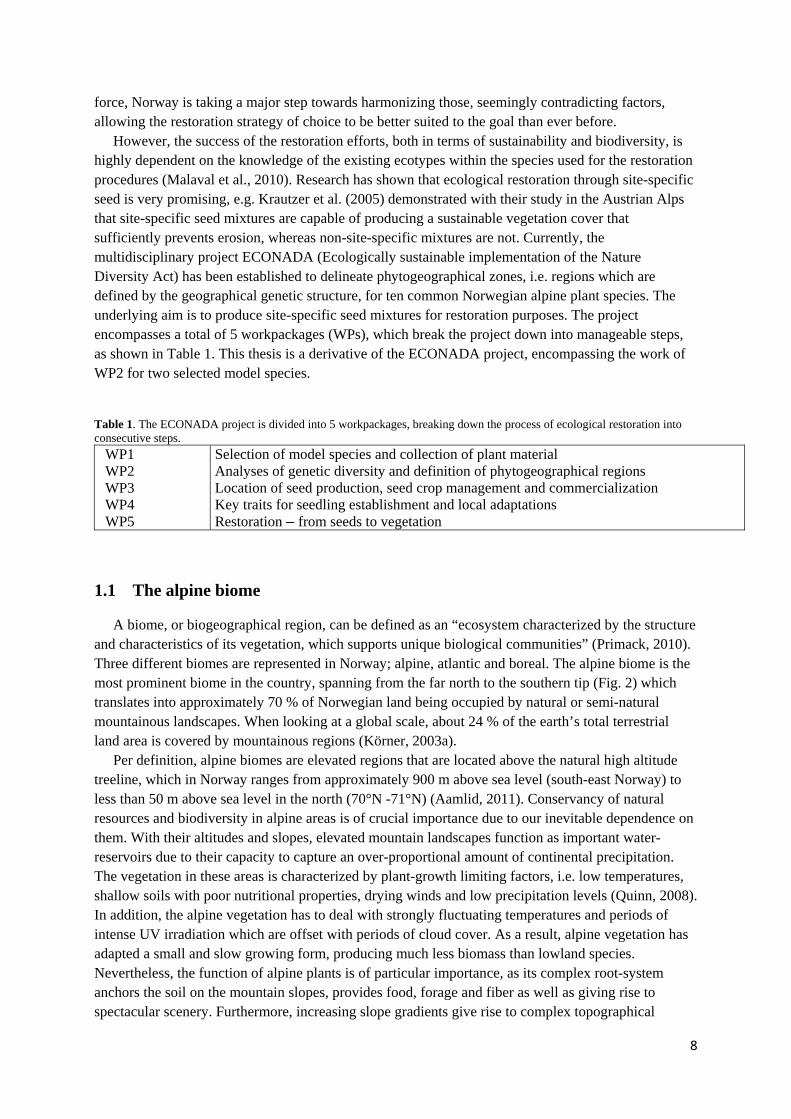
However, the success of the restoration efforts, both in terms of sustainability and biodiversity, is highly dependent on the knowledge of the existing ecotypes within the species used for the restoration procedures (Malaval et al., 2010). Research has shown that ecological restoration through site-specific seed is very promising, e.g. Krautzer et al. (2005) demonstrated with their study in the Austrian Alps that site-specific seed mixtures are capable of producing a sustainable vegetation cover that sufficiently prevents erosion, whereas non-site-specific mixtures are not. Currently, the multidisciplinary project ECONADA (Ecologically sustainable implementation of the Nature Diversity Act) has been established to delineate phytogeographical zones, i.e. regions which are defined by the geographical genetic structure, for ten common Norwegian alpine plant species. The underlying aim is to produce site-specific seed mixtures for restoration purposes. The project encompasses a total of 5 workpackages (WPs), which break the project down into manageable steps, as shown in Table 1. This thesis is a derivative of the ECONADA project, encompassing the work of WP2 for two selected model species.

Table 1. The ECONADA project is divided into 5 workpackages, breaking down the process of ecological restoration into consecutive steps.

WP1 WP2 WP3 WP4 WP5

Selection of model species and collection of plant material Analyses of genetic diversity and definition of phytogeographical regions Location of seed production, seed crop management and commercialization Key traits for seedling establishment and local adaptations Restoration – from seeds to vegetation

1.1 The alpine biome

A biome, or biogeographical region, can be defined as an “ecosystem characterized by the structure and characteristics of its vegetation, which supports unique biological communities” (Primack, 2010). Three different biomes are represented in Norway; alpine, atlantic and boreal. The alpine biome is the most prominent biome in the country, spanning from the far north to the southern tip (Fig. 2) which translates into approximately 70 % of Norwegian land being occupied by natural or semi-natural mountainous landscapes. When looking at a global scale, about 24 % of the earth’s total terrestrial land area is covered by mountainous regions (Körner, 2003a).

Per definition, alpine biomes are elevated regions that are located above the natural high altitude treeline, which in Norway ranges from approximately 900 m above sea level (south-east Norway) to less than 50 m above sea level in the north (70°N -71°N) (Aamlid, 2011). Conservancy of natural resources and biodiversity in alpine areas is of crucial importance due to our inevitable dependence on them. With their altitudes and slopes, elevated mountain landscapes function as important water-reservoirs due to their capacity to capture an over-proportional amount of continental precipitation. The vegetation in these areas is characterized by plant-growth limiting factors, i.e. low temperatures, shallow soils with poor nutritional properties, drying winds and low precipitation levels (Quinn, 2008). In addition, the alpine vegetation has to deal with strongly fluctuating temperatures and periods of intense UV irradiation which are offset with periods of cloud cover. As a result, alpine vegetation has adapted a small and slow growing form, producing much less biomass than lowland species. Nevertheless, the function of alpine plants is of particular importance, as its complex root-system anchors the soil on the mountain slopes, provides food, forage and fiber as well as giving rise to spectacular scenery. Furthermore, increasing slope gradients give rise to complex topographical

8  

structure in the terrain, allowing for an abundance of diverse alpine microhabitats (Körner, 2003b) that enable a level of biodiversity richness which exceeds many lowland ecosystems (Körner, 2003a).

 Figure 2. Biogeographical regions of Europe: note the large area of Norway covered by the alpine biome (European Environment Agency (2005))

Unfortunately, alpine ecosystems are changing due to factors as increasing infrastructure, agriculture and forestry, recreation, nitrogen deposition and invasive species (Nigel et al., 2010). Due to the extreme environmental conditions of the alpine zone, restoration efforts of damaged sites are of particular interest as natural recovery in such ecosystems, is often a very slow and problematic process (Malaval et al., 2010). The need for active measures to increase the recovery rates of disturbed ecosystems has already been recognized for several decades. Yet, the choice of restoration tactics is often restricted due to the associated high costs. Consequently, cheap restoration methods and low cost commercial seed mixtures are often implemented (Tamegger and Krautzer, 2006). Therefore, neither the required levels of genetic diversity needed for a sustainable recovery process, nor questions regarding spatial genetic structure (SGS) and adaptation patterns, are taken into account (McKay et al., 2005). Successes of such efforts are often low due to reduced viability of the alien species and lowered biodiversity (Malaval et al., 2010), while correlated negative effects such as soil erosion, more surface

9  

drainage and original flora impurity cause comprehensive ecological and economical damage (Tamegger and Krautzer, 2006). Additionally, seedling establishment of such alien species can be difficult as well. Insight in the SGS of native alpine plants is therefore a much needed requirement in order to establish site-specific seed mixes based on the geographical genetic structures of native alpine plant species.

1.2 Challenges in Norwegian mountain areas

Norwegian landscapes have a rich cultural history. Although the alpine regions have only been sparsely populated, traditional low intensity summer farming practices have shaped the landscape for thousands of years. In the 19th century, as many as 70 000 summer farms were in operation throughout the country, gently crafting a species-rich semi-natural montane ecosystem (Norderhaug and Sickel, 2007). Modern high intensity farming methods lead to the abandonment of the vast majority of these typical Norwegian summer farms, leaving the meadows in an unbalanced state. Tourism, infrastructure and hydro-electric constructions are other major disturbance factors (Norderhaug and Sickel, 2007). Such disturbances have a detrimental effect on the alpine ecosystem, especially because the environmental conditions do not allow for rapid recovery. Therefore, ecological restoration is highly desired in order to retain ecosystem functionality and maintain biodiversity and natural resources.

1.3 Site-specific Seed

The Nature Diversity Act, which was passed by the Norwegian Parliament on the 19th of June 2009, addresses the risk of genetic pollution in natural areas and has prohibited the introduction of alien organisms, i.e. organisms which do not belong to a species or population naturally occurring in an area, into nature (Government Administration Services, 2009). Furthermore, the Act promotes the use of site-specific seed, which implies that samples from one region should not be introduced in another region unless genetic similarity has been confirmed (Aamlid, 2011), giving rise to the need for the definition of seed transfer zones. In response, commercial seed production and genetic diversity investigations of native alpine species have begun, starting with an economical evaluation of suitable candidate species.

Compared to cultivated species, seed production of native alpine plants is much more risky and costly, due to their slow growth and development and weak competitiveness (Krautzer et al., 2004). In order to establish profitable businesses, production requirements and seed availability of the site-specific plants must be carefully considered. Seedbed preparation, susceptibility to diseases and weed invasions, seed development requirements and harvesting techniques are all potential decisive factors. Once species have been identified in terms of their suitability for restoration and economic seed production prospects, the use of neutral genetic markers, such as AFLPs, potentially leads to the zonation of the area into several genetically distinct zones and the levels of genetic diversity within them. Seed growers, ecologists and plant physiologists can use these zones of genetic relatedness as a basis for a new testing procedure in which local adaptations (that are also genetic but are not being picked up by neutral genetic marker technology) are being explored. At that stage, numerous tests should be carried out to learn about the species’ particular adaptations or its use of phenotypic plasticity, ultimately leading to a clear delineation of seed transfer zones and establishments of seed production sites that are well suited to meet the requirements of the particular alpine species.

10  

1.4 Genetic Variation

Genetic variation describes genetic differences within and between populations. It is the key to local adaptation and mutation is the ultimate source of it. Gene flow, random genetic drift and natural selection are the ultimate forces that shape the patterns of genetic differentiation within a species. Patterns of gene flow depend on many variable factors, such as mating strategy, seed dispersal and establishment, population density (Hamrick and Nason, 1996) and microhabitat selection (Trapnell et al., 2008). The spatial distribution of genetic variation within populations is mostly controlled by seed dispersal patterns and seedling establishment rates (Nason and Hamrick, 1997). Clonal growth is also impacting geographical genetic structure, because this form of reproduction results in an increase of individuals of the same genotype in a population and therefore also increases the sexual reproductive potential of this genotype. Depending on the efficiency of seed dispersal and seed establishment, clonal growth has the potential to lower the genetic variability on both intra- and interpopulation levels.

Genetic variation among populations is mostly shaped by limitations in gene flow between populations and genetic drift within populations. Environmental factors, such as average length and temperature of the growing season, amount of available daylight, soil composition and seasonal precipitation patterns can act as barriers for gene flow. Topographic relief and altitudinal differences are known to have a negative impact on gene flow in a wide variety of species, as reviewed by Storfer et al. (2010). Simply put, when cross-pollination and seed dispersal is ineffective in reaching adjacent populations, genes are not being transferred between these populations and hence become more distinct.

An important point to address is that historical limitations in gene flow have a large effect on the modern day genetic structure within a species. In the Norwegian mountain setting, glacial retreats and advances have occurred repeatedly (Nesje et al., 2008), likely to have structured genetic variation among populations due to allowance of plant migration in times of glacial retreat and stationary periods when covered by glacial ice sheets. Postglacial expansion may lead to isolation by distance (IBD), which is defined as “a decrease in the genetic similarity among populations as the geographic distance between them increases” (Jensen et al., 2005) and is frequently occurring in species. If IBD is present in a species, distinguished geographical genetic structures can be identified: each structural unit represents a zone that is genetically different from one another.

1.5 Use of molecular markers in land management and conservation efforts

Molecular markers are useful tools to extract large quantities of biological information. They can be viewed as flags or landmarks within the genome of an organism, based on differences in DNA sequence between individuals. Molecular markers are generally neutral and hence unaffected by natural selection which makes them suitable indicators for gene flow and genetic drift, but it should be kept in mind that such information does not necessarily lead to increased apprehension of a species’ adaptability (McKay et al., 2005). Through the pressure of all active evolutionary forces on a population, distinct genetic patterns may form within and/or between populations. Based on the abundance of variation in the genetic code even within a species, each plant has an individual “fingerprint” which makes marker technology extremely powerful.

The advancement of marker technology has yielded a wide array of DNA-based marker technologies, e.g. amplified fragment length polymorphisms (AFLPs), microsatellites and single nucleotide polymorphisms (SNPs). Costs of highly advanced sequencing methods have decreased in

11  

such a fashion, that genotyping-by-sequencing is now feasible for a wide variety of genomes of highly diverse species (Elshire et al., 2011). Landscape-genetics, molecular ecology and conservation work require markers that capture a medium to high amount of polymorphisms to be able to infer inter- and intrapopulation variation in the studied organism. From a review by Anderson et al. (2010), it became evident that microsatellites are used most in the field of landscape genetics, but amplified fragment

length polymorphisms (AFLPs) and organellar DNA sequences (chloroplast ͂ [cpDNA] and mitochondrial mtDNA) are also frequently used. Previously, randomly amplified DNA markers (RAPDs) were common in such studies, but they have declined due to their questioned reproducibility.

Since the range of available marker technologies is rather extensive, researchers have to carefully weigh the advantages and disadvantages of each suitable method. These considerations should be based on both the biological aspects of the particular study, the proposed research questions and the available resources (Meudt and Clarke, 2007). Furthermore, a review by Anderson et al. (2010) recommends that the time scales, over which the genetic variation has accumulated, should also be considered, as well as mutation rates.

For genetic profiling of plants as part of land management, conservation or restoration efforts, PCR profiling based methods, like AFLPs, are often preferred due to the mere fact that they only require small amounts of DNA, are relatively inexpensive and do not require any priori sequence knowledge. This sets them apart from both SNPs and microsatellites, which do require sequence information and are potentially more costly because researchers first have to invest time and resources into the making of a species library, which is not always necessary. In that case, AFLPs may be the preferred choice. For questions regarding historical changes in genetic patterns, cpDNA can provide excellent markers due to their slower evolutionary rate of such DNA (e.g. Fjellheim et al., in prep.). However, such markers are not recommended for land management and restoration issues.

In their detailed overview of 11 molecular marker techniques, Semagn et al. (2006), concluded that AFLP is both highly reliable and reproducible and also has the potential to yield a high amount of polymorphic markers. On the downside, AFLPs are dominant markers, meaning that dominant homozygotes cannot be distinguished from heterozygotes, which could complicate the analysis regarding population genetics or genetic diversity studies. However, other than the usual binary scoring of AFLP data, codominant genotype calling may be possible when it can be assumed that the intensity of the marker is a direct measure for the amount of DNA amplified (Gort and Van Eeuwijk, 2010). Yet, binary scoring is sufficient for studies contributing to the development of site-specific seed mixtures, because data on the mere presence or absence of alleles per population is required. Considering all above, AFLP is the molecular marker of choice for this study as it does not require any prior knowledge of the genomic sequence, and besides, it is highly reproducible and reveals many polymorphic loci throughout the entire genome.

1.6 The AFLP technique

The molecular fingerprinting technique called AFLP (Amplified Fragment Length Polymorphism) has proven its usefulness during the years, particularly in ecological, evolutionary and conservation studies (Caballero and Quesada, 2010). The method was initiated by KeyGene N.V. (Vos et al., 1995) and consists of a procedure which involves five major steps as nicely outlined by Chial (2008). First, genomic DNA must be isolated from each individual sample and a pair of restriction enzymes is exploited to fully digest the genomic DNA. The restriction enzymes are a carefully chosen pair of a frequent cutter (recognizes a 4 base pair sequence) and a rare cutter (recognizes a 6 base pair sequence), such as MseI and EcoRI respectively and are given sufficient incubation time to ensure complete digestion of total genomic DNA. After cleavage with the two restriction enzymes, three

12  

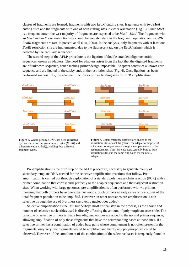
classes of fragments are formed: fragments with two EcoRI cutting sites, fragments with two MseI cutting sites and the fragments with one of both cutting sites in either orientation (Fig. 3). Since MseI is a frequent cutter, the vast majority of fragments are expected to be MseI - MseI. The fragments with an MseI and an EcoRI restriction site should be less abundant in the fragment population and EcoRI-EcoRI fragments are rare, if present at all (Liu, 2004). In the analysis, only fragments with at least one EcoRI restriction site are implemented, due to the fluorescent tag on the EcoRI primer which is detected by the capillary sequencer.

The second step of the AFLP procedure is the ligation of double stranded oligonucleotide sequences known as adapters. The need for adapters arises from the fact that the digested fragments are of unknown sequence, hence making primer design impossible. Adapters consist of a known core sequence and are ligated to the sticky ends at the restriction sites (Fig. 4). Once ligation has been performed successfully, the adapters function as primer binding sites for PCR amplification.

Figure 3. Whole genomic DNA has been restricted by two restriction enzymes (a rare cutter (EcoRI) and a frequent cutter (MseI)), yielding four different fragment types.

Figure 4. Complementory adapters are ligated to the restriction sites of each fragment. The adapters comprise of a known core sequence and a region complementary to the restriction sites. Thus, Mse adapters can only bind to Mse restriction sites and the same rule holds for the EcoRI adapters

Pre-amplification is the third step of the AFLP procedure, necessary to generate plenty of

secondary template DNA needed for the selective amplification reactions that follow. Pre-amplification is carried out through exploitation of a standard polymerase chain reaction (PCR) with a primer combination that corresponds perfectly to the adapter sequences and their adjacent restriction sites. When working with large genomes, pre-amplification is often performed with +1 primers, meaning that both primers have one extra nucleotide. Such primers already cause only a subset of the total fragment population to be amplified. However, in other occasions pre-amplification is non-selective through the use of 0-primers (zero extra nucleotides added).

Selective amplification is the last, but perhaps most critical step in the process, as the choice and number of selective nucleotides used is directly affecting the amount of polymorphism accessible. The principle of selective primers is that a few oligonucleotides are added to the normal primer sequence, allowing amplification of only those fragments that have the corresponding bases at those sites. If a selective primer has a combination of added base pairs whose complement is not often present in the fragments, only very few fragments would be amplified and hardly any polymorphism could be observed. However, if the compliment of the combination of the selective bases is frequently found in

13  

the fragments, many fragments would be amplified, hence giving access to much more polymorphic sites.

1.7 Statistical tools for AFLP data

Without statistical tools, it is impossible to comprehend the biological meaning of the acquired genetic data. To be able to answer the research questions, several statistical tools must be applied. For the analysis of AFLP data, two kinds of methods are available. The first approach is band-based, thus involves the direct study of fragment presence or absence, while the other approach relies on an estimation of allele frequencies within populations and therefore is population-based.

1.7.1 Principal Coordinates Analysis

Multivariate analyses have the ability to translate multivariate genetic data into a small amount of variables. Principal coordinate analysis (PCoA or PCO) is an appropriate multivariate analyzing tool when genetic structuring among populations needs to be inferred from a genetic data matrix. A PCO works well for a vast array of genetic markers, including AFLPs (Toro and Caballero, 2005). The basic principle behind a PCO for genetic exploitations is nicely reviewed by Jombart et al. (2009) and to promote the coherence and readability of this text, a short summary is included here. For each object, the genetic information acquired from p genetic markers is placed in a p dimensional space. By doing so, each object receives a set of coordinates, also known as principal components, or eigenvectors, which can be further deduced to measures that quantify the variation within the component, called eigenvalues. When these quantified variables are plotted over the principal axis, i.e. the directions that explain most variability within the data set, any hidden genetic structuring may become visible.

1.7.2 Bayesian Analysis of Population Structure

Bayesian clustering approaches are increasingly being used for many biological questions as summarized in a short communications article by Latch et al. (2006). In this study, the method is used to infer insight in the molecular organization within the data set, which could help to gain insight in phytogeographical zones and therefore validate the outcome of the PCO analysis. Bayesian methodology is becoming increasingly implemented in the field of landscape genetics, although it assumes the strictly theoretical phenomenon of Hardy-Weinberg equilibrium, neutral markers and thus also linkage equilibrium. The Bayesian clustering methodology is based on the placements of the analysed individuals into K groups, in such a way that the individuals within each group have the most similar genotypes and the groups themselves are as close to HWE as possible (Corander et al., 2008).

1.7.3 Analysis of Molecular Variance

The amount of genetic structure can be investigated with an Analysis of Molecular Variance (AMOVA), as described by Excoffier et al. (1992). Several variations of the technique are implemented in Arlequin software (Excoffier and Lischer, 2010), such as the Standard AMOVA and the Locus-by-Locus AMOVA. The backbone of the two methods is that the data has to be classified in groupings of genetic relatedness, usually as obtained from a multivariate analysis or Bayesian

14  

clustering approach. The AMOVA will then test this predefined genetic structure in order to partition the total genetic variance into covariance components, based on differences among groups, among populations and within populations. In the standard AMOVA, the test is performed on the haplotype level, while the Locus-by-Locus approach is performed separately for each locus. To gain insight in the exact calculations, the Arlequin 3.5.software manual provides all the requested data.

1.7.4 Gene diversity measures

The previously statistical procedures are implemented to enable the delineation of seed transfer zones per species and to learn which ecotypes should be included in each seed mixture. However, those methods do not quantify the genetic variation within and between populations, which is also of crucial importance. Not only is it necessary to find the gene diversity within populations to find the most viable sources for commercial seed production, but it also functions as a quality control measure for restoration projects. Gene diversity in our datasets was measured with two different measurements. First, Nei’s gene diversity (D) is calculated for each population, using the equation

D = n/(n-1) * [1 – (freq1

2 + freq0

2)]

n = the number of individuals

freq12 = amount of present fragments of a particular

marker in a population freq0

2 = amount of absent fragments of a particular marker in a population

for each marker and then taking the average (Nei, 1987). Secondly, another measure for gene diversity was exploited, i.e. the “frequency-down-weighted marker values” (DW), which was calculated by, for each population, dividing the number of “present” scores of each AFLP marker within a population by the total amount of “present” scores of that marker in the entire dataset and, subsequently, summing those values per marker up to obtain the DW for each population (Schönswetter and Tribsch, 2005).

 

1.8 Description of species

1.8.1 Phleum alpinum

The genus Phleum encompasses approximately 14 different species, of which P. pratense is the most famous as it is a commonly used forage and hay crop in the cold temperate regions of the world (Stewart et al., 2011). Taxonomically, P. alpinum is rather challenging, as there are occasional different polyploid forms within the species whose names and identities are not always agreed upon across taxonomists. In northern Scandinavia, however, only the tetraploid form has been reported and hence the name P. alpinum is here assigned to the tetraploid taxon (Elven et al., 2005).

P. alpinum L., more commonly known as Alpine timothy or Alpine cat’s tail, is a small (10 to 30 cm tall) perennial bunchgrass (Fig. 5) belonging to the Poaceae family. The origin of the species lies in Asia, where over 300,000 years BP an unknown genome hybridized with an ancestral genome of P. alpinum L. subsp. rhaeticum. This hybrid eventually migrated into Europe after the last glacial period

15  

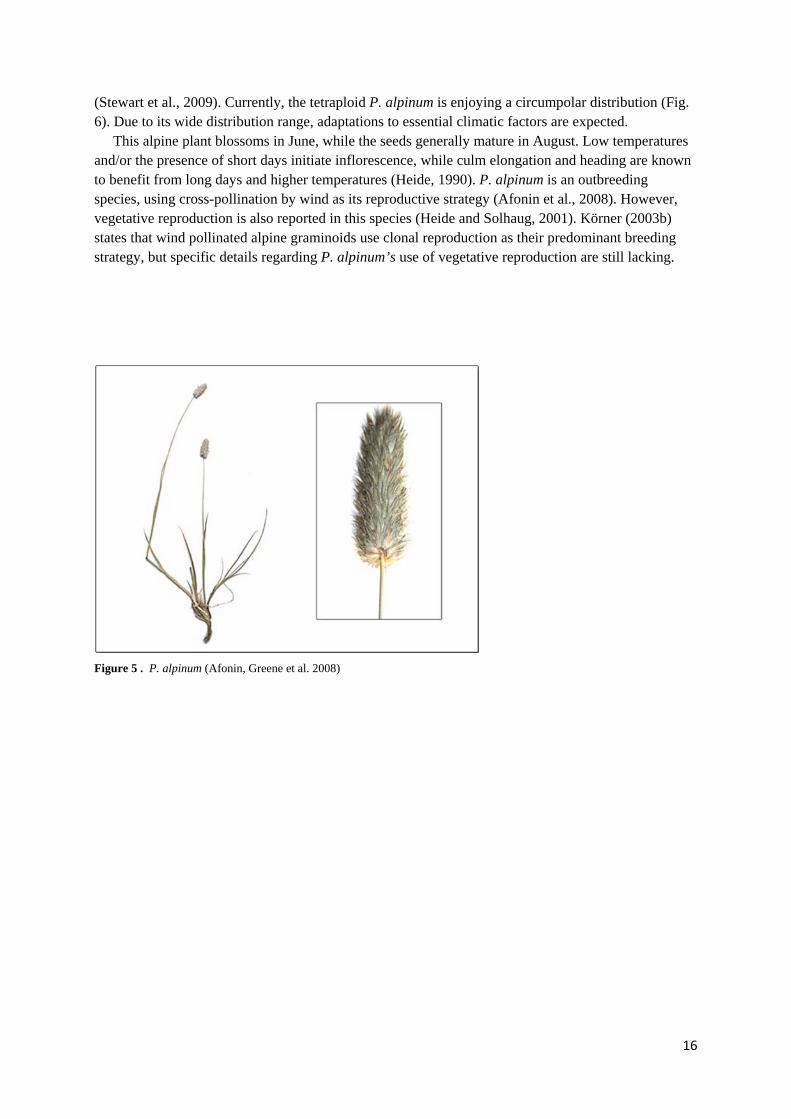
(Stewart et al., 2009). Currently, the tetraploid P. alpinum is enjoying a circumpolar distribution (Fig. 6). Due to its wide distribution range, adaptations to essential climatic factors are expected.

This alpine plant blossoms in June, while the seeds generally mature in August. Low temperatures and/or the presence of short days initiate inflorescence, while culm elongation and heading are known to benefit from long days and higher temperatures (Heide, 1990). P. alpinum is an outbreeding species, using cross-pollination by wind as its reproductive strategy (Afonin et al., 2008). However, vegetative reproduction is also reported in this species (Heide and Solhaug, 2001). Körner (2003b) states that wind pollinated alpine graminoids use clonal reproduction as their predominant breeding strategy, but specific details regarding P. alpinum’s use of vegetative reproduction are still lacking.

 Figure 5 . P. alpinum (Afonin, Greene et al. 2008)

16  

 Figure 6. Distribution of P. alpinum in the Northern Hemisphere (Hultén and Fries 1986).

1.8.2 Leontodon autumnalis

The genus Leontodon, within the Asteraceae family, has also had a “bewildering history” until Bentham gave it a rather wide definition in 1873 (Greunter et al., 2006). The genus includes about 50 species (Yurukova-Grancharova, 2004), but Greunter et al. (2006) suggest that L. subg. oporonia to which Leontodon autumnalis belongs, should be placed under the genus Scorzoneroides based on molecular investigations by Samuel et. al. (2006). There are now two possible names for the species, i.e. Leontodon autumnalis L. and Scorzoneroides autumnalis (L.) Moench, and it is not truly clear if consensus for the correct name has been reached yet. In this thesis, traditional name L. autumnalis has been kept. The common names of this species are Fall Dandelion or Autumn Hawkbit.

L. autumnalis is a small (20 -30 cm) long lived, diploid perennial herb that is native to Eurasia, and has been introduced in North America and New Zealand (Fig. 7). It is a diploid species (2n = 12) (Yurukova-Grancharova 2004) that produces one or two branched stems, capable of carrying two or more bright yellow flowerheads (Fig. 8). The leaves are deeply lobed and form a basal rosette (Fig. 9) around the single or few branched stems (Picó and Koubek, 2003). Individual plants can either have hairy or glabrous leaves. Reproduction occurs through insect pollination, using mainly flies as they are the most frequent visitors in alpine regions (Totland, 1993). Selfing is not an issue in this species; Picó et al. (2003) demonstrated that L. autumnalis has a compelling self-incompatibility system.

17  

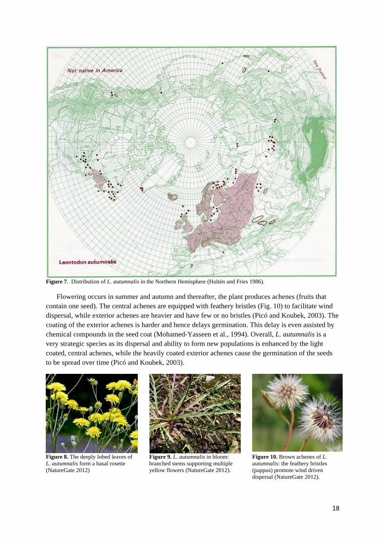
Figure 7. Distribution of L. autumnalis in the Northern Hemisphere (Hultén and Fries 1986).

Flowering occurs in summer and autumn and thereafter, the plant produces achenes (fruits that contain one seed). The central achenes are equipped with feathery bristles (Fig. 10) to facilitate wind dispersal, while exterior achenes are heavier and have few or no bristles (Picó and Koubek, 2003). The coating of the exterior achenes is harder and hence delays germination. This delay is even assisted by chemical compounds in the seed coat (Mohamed-Yasseen et al., 1994). Overall, L. autumnalis is a very strategic species as its dispersal and ability to form new populations is enhanced by the light coated, central achenes, while the heavily coated exterior achenes cause the germination of the seeds to be spread over time (Picó and Koubek, 2003).  

   

Figure 8. The deeply lobed leaves of L. autumnalis form a basal rosette (NatureGate 2012) 

  Figure 9. L. autumnalis in bloom: branched stems supporting multiple yellow flowers (NatureGate 2012).

  Figure 10. Brown achenes of L. autumnalis: the feathery bristles (pappus) promote wind driven dispersal (NatureGate 2012).

  

18  

1.9 Research objective

In this study, two alpine plant species were assessed for their spatial genetic structure throughout Norway, using AFLP markers. The species, Phleum alpinum and Leontodon autumnalis, were sampled from 20 locations throughout Norway, so that seed transfer zones within the country can be delineated for both species. Eventually, the information acquired in this thesis will contribute to the establishment of site-specific seed mixtures. The research questions are formulated below in a more specific manner:

Are the populations genetically different from each another? What are the patterns of variation? What are the underlying reasons for these patterns? Can we delineate seed transfer zones? How can the acquired information be applied?

To our knowledge, this is the first study in which the AFLP technique has been performed on P.

alpinum and L. autumnalis. Yet, genetic structuring of L. autumnalis has previously been investigated with RAPD markers in a study in Central Europe (Grass et al., 2006).

19  

2. Methodology

2.1 Sample collection

According to the work schedule of the ECONADA project, samples were collected from June to September 2011, following the guidelines listed below:

Samples should not be collected from an area where previous seeding or introduction of the species may have occurred as result of revegetation, agricultural use or any other activity;

From each species, materials from 20 individuals should be collected in each of the 20 collection sites;

The individuals chosen for sampling must grow at least 5-10 m apart;

The collected plant material (leaves / stems) must be fresh and green with no signs of disease or fungal infection (avoid leaves with spots, faded areas, etc.). Seeds and flowers should not be collected;

Care should be taken to ensure material from only one individual is placed in each bag.

Permission was granted to use all samples of P. alpinum and L. autumnalis which had been collected. Samples were taken from 20 locations, distributed over Norway’s total land area (Fig. 9). The complete instructions for sampling and handling can be found in Appendix VII (in Norwegian).

20  

Figure 9. Sampling locations.

Per location, material from 20 individual plants per species was sampled. Coordinates for the sampling locations where approximated with Google Earth (Google Inc., 2012), and can be found in Table 2. Due to different samplers per region, some samples had plenty of leaf material, while other samples were small and without leaves. For this study, the leaf material was preferred, but occasionally stems were utilized when leaf material was not present or insufficient. Flowers and seeds were avoided, as they resemble the next generation. After collection, the samples were stored in

21  

individual zip-lock bags containing silica gel. All bags were properly labeled and organized according to species and location.

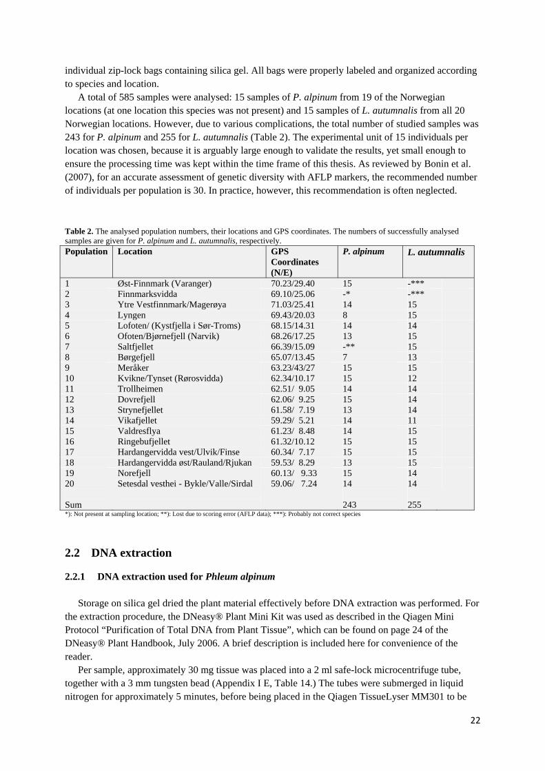
A total of 585 samples were analysed: 15 samples of P. alpinum from 19 of the Norwegian locations (at one location this species was not present) and 15 samples of L. autumnalis from all 20 Norwegian locations. However, due to various complications, the total number of studied samples was 243 for P. alpinum and 255 for L. autumnalis (Table 2). The experimental unit of 15 individuals per location was chosen, because it is arguably large enough to validate the results, yet small enough to ensure the processing time was kept within the time frame of this thesis. As reviewed by Bonin et al. (2007), for an accurate assessment of genetic diversity with AFLP markers, the recommended number of individuals per population is 30. In practice, however, this recommendation is often neglected.

 

Table 2. The analysed population numbers, their locations and GPS coordinates. The numbers of successfully analysed samples are given for P. alpinum and L. autumnalis, respectively. Population

Location GPS Coordinates (N/E)

P. alpinum L. autumnalis

1 Øst-Finnmark (Varanger) 70.23/29.40 15 -*** 2 Finnmarksvidda 69.10/25.06 -* -*** 3 Ytre Vestfinnmark/Magerøya 71.03/25.41 14 15 4 Lyngen 69.43/20.03 8 15 5 Lofoten/ (Kystfjella i Sør-Troms) 68.15/14.31 14 14 6 Ofoten/Bjørnefjell (Narvik) 68.26/17.25 13 15 7 Saltfjellet 66.39/15.09 -** 15 8 Børgefjell 65.07/13.45 7 13 9 Meråker 63.23/43/27 15 15 10 Kvikne/Tynset (Rørosvidda) 62.34/10.17 15 12 11 Trollheimen 62.51/ 9.05 14 14 12 Dovrefjell 62.06/ 9.25 15 14 13 Strynefjellet 61.58/ 7.19 13 14 14 Vikafjellet 59.29/ 5.21 14 11 15 Valdresflya 61.23/ 8.48 14 15 16 Ringebufjellet 61.32/10.12 15 15 17 Hardangervidda vest/Ulvik/Finse 60.34/ 7.17 15 15 18 Hardangervidda øst/Rauland/Rjukan 59.53/ 8.29 13 15 19 Norefjell 60.13/ 9.33 15 14 20 Sum

Setesdal vesthei - Bykle/Valle/Sirdal

59.06/ 7.24 14 243

14 255

*): Not present at sampling location; **): Lost due to scoring error (AFLP data); ***): Probably not correct species

2.2 DNA extraction

2.2.1 DNA extraction used for Phleum alpinum

Storage on silica gel dried the plant material effectively before DNA extraction was performed. For the extraction procedure, the DNeasy® Plant Mini Kit was used as described in the Qiagen Mini Protocol “Purification of Total DNA from Plant Tissue”, which can be found on page 24 of the DNeasy® Plant Handbook, July 2006. A brief description is included here for convenience of the reader.

Per sample, approximately 30 mg tissue was placed into a 2 ml safe-lock microcentrifuge tube, together with a 3 mm tungsten bead (Appendix I E, Table 14.) The tubes were submerged in liquid nitrogen for approximately 5 minutes, before being placed in the Qiagen TissueLyser MM301 to be

22  

grinded for 1 minute at 30 Hz. The samples were checked immediately to ensure proper disruption of the plant material. To ensure proper homogenization of the material, samples were returned to the Qiagen TissueLyser for 30-60 seconds, depending on the state of disruption. The TissueLyser breaks the cell walls and homogenizes the sample, hence allowing proper lysation.

All samples were again submerged in liquid nitrogen and respectively placed on ice before adding 400 µl AP1 buffer to each tube. Additional AP1 was added if necessary to remove clumps. Then 4 µl RNase was added, after which the sample was vortexed immediately and placed on ice to keep the enzymes dormant. Then, the samples were incubated in a 65ºC water bath for 10 minutes. The tubes were inverted three times during the incubation time, to optimize lysis of all cells.

To precipitate proteins, polysaccharides and detergents, 130 µl of AP2 buffer was added to each tube individually, followed by vortexing and placing the sample on ice immediately afterwards. The samples were incubated on ice for at least 5 minutes, before centrifuging for 6 minutes at 13000 rpm. The lysate was pipetted in the Qiaschredder Mini Spin Column, which was then centrifuged for 2 minutes at 13000 rpm. The flow-through was transferred to a new tube and the appropriate amount of prepared AP3/E buffer was added followed by gentle mixing by a few gentle inversions. Divided into two steps, the newly acquired mixture was centrifuged through the membrane of the DNeasy Mini Spin Column, to bind the DNA to the membrane.

Additionally, to wash any debris from the membrane, 500 µl AW buffer was added when the DNeasy Mini Spin Column had been placed on a new 2ml collection tube and the sample was centrifuged for 1 minute at 8000 rpm. Another wash was performed for 2 minutes at 13000 rpm. Then, the Spin Column was carefully transferred onto a new microcentrifuge tube and left to dry at room temperature with open lid.

To release the DNA from the membrane, 100 µl AE buffer at 65ºC was pipetted onto the membrane. In the case of very small sample sizes, 50 µl AE buffer was used. The tubes were incubated for 5 min. at room temperature and then centrifuged for 1 min. at 8000 rpm. This DNA solution was then appropriately marked as Elution I and immediately placed in the freezer at -20ºC. Another elution was performed to release the remaining DNA. This was stored accordingly as Elution II. The quantity and quality of the obtained DNA was always tested on a 1 % agarose gel (subchapter 2.3).

2.2.2 DNA extraction used for Leontodon autumnalis

To increase efficiency, the genomic DNA of the dried samples of L. autumnalis was isolated with the Omega Biotek E-Z 96 Plant DNA Kit. The Plant DNA Centrifugation Protocol was used as outlined in the accompanied manual. As some slight modifications were made, a brief description of the procedure follows.

First, an outline of the 96-well plate was made to allocate each plant to a well location on the plate. Following this outline, approximately 35 mg of dried plant material was placed in each well, using a sterile pincet which was treated with absolute ethanol between each sample. If a sample appeared to be of low quality, a replacement sample was taken and the outline of the 96 well plate was immediately adjusted. A 3 mm tungsten carbide bead was added to all wells for disruption of the samples in the homogenizer. The wells of the plate were properly closed before placing it in liquid nitrogen to freeze the samples. Then, the plates were homogenized for 2 times 1 minute in the Qiagen TissueLyser MM301, starting at a frequency of 20 Hz and increasing to 30 Hz both times.

After proper disruption of the samples, the plates were centrifuged for 1 minute at 4000 rpm to spin the powder to the bottom before opening to add 400 µl of the RNase A treated SP1 solution. The plates were then vortexed thoroughly to dissolve the samples properly. When all powder had

23  

dissolved, the plates were incubated in a 65°C waterbath for 15 minutes, mixing the samples every 3 minutes. Once the incubation time had passed, the plates were centrifuged briefly and 140 µl SP2 buffer was added to each lysate. Again, the plates were vortexed and then incubated at room temperature to precipitate proteins, polysaccharide and other enzyme inhibiting compounds. After the incubation period, the plates were centrifuged for 10 minutes at 6000 x g. The supernatants were then transferred to the racked microtubes and the prescribed volume of SP3 (prepared with ethanol) was added to each well. The racked microtubes were vortexed and centrifuged according to the protocol.

The supernatants were transferred to the HiBind DNA Plate, which had been treated with the equilibrium buffer as the protocol described. The plates were sealed with the AeraSeal film and centrifuged for 5 minutes at 5000 x g. Sometimes additional centrifugation time was added to allow all sample fluid to pass through the membrane. The flow-through was discarded from the Deep Well collection plate and then the HiBind was filled with 800 µl SPW Wash buffer. Again, the plate was sealed and centrifuged at 5000 x g for 5 minutes. The flow through was removed and this step was repeated, but this time centrifuged for 2 cycles of 5 minutes (discarding the flow-through after each session). The tubes were opened after the second session to air-dry.

Finally, the DNA was eluted with 100 µl Elution buffer (65°C). After adding the buffer, we incubated the plates for 5 minutes at room temperature and centrifuged for 5 minutes at 5000 x g afterwards. The second elution was performed likewise. The extracted DNA was tested on 1 % agarose gels and was then stored in the freezer (-20°C).

2.3 Gel electrophoresis

Gel electrophoresis was used extensively to ensure the products of the work were sufficient to continue, or to be able to evaluate the quantity of the genomic DNA. All electrophoreses were performed on 1 % agarose gels, which were prepared in the following manner:

1. For a large 1 % gel, 250 ml 1x TBE buffer and 2.5 g agarose were combined in a flask and heated in a microwave oven until the powder was fully dissolved;

2. The flask was then retrieved from the microwave and cooled until lukewarm, before adding one drop of 0.07 % ethidium bromide (EtBr) per 50 ml to a final concentration of 0.5µg/ml;

3. The solution was then poured in a gel tray with one or more loading combs and left to set;

4. Once the gel was ready, the combs were removed and the gel was placed in a electrophoresis tray;

5. The samples to be analysed were prepared with loading buffer and pipetted onto the gel together with a 1kb molecular ladder;

6. The voltage and running time were variable, depending on the gel size and the space between rows of samples;

7. To visualize the results, the gels were placed under UV light in a Gel Doc™ EQ Universal Hood II (BioRad Laboratories, Segrate, Italy) and analysed by Quantity One® software.

2.4 Digestion of whole genomic DNA

In this study, the rare cutting enzyme EcoRI (6-bp recognition sequence) and the frequent cutter MseI (4-bp recognition sequence) were used for the digestion of whole genomic DNA. These are

24  

typical enzymes for AFLP marker technology. Using the 1kb ladder, the quantities of genomic DNA were estimated and volumes containing approximately 250 ng genomic DNA were calculated. Then, the volumes of dH2O, needed to increase the total volume to 30 µl, were recorded. In a 96-well PCR plate, first the volumes of water were pipetted into the appropriate wells, followed by the complimentary volumes of DNA of the strongest elution. The digestion mix contained 0.25 µl EcoRI, 0.5 µl MseI, 8.0 µl 5x RL+ buffer and 1.25 µl dH2O per sample and 9.5 µl of this was added to the wells for the cleavage reaction. The plate was kept on ice during the procedure. Once the “digestion mix” was added, the plate was closed with domed caps and sealed with Parafilm, before being placed for 2.5 hours in a 37 ºC water bath. To ensure proper cleavage of the DNA had occurred, 10 µl of the digested DNA was tested on a 1 % agarose gel. The remaining 30 µl was used in ligation.

2.5 Extra purification of DNA

One hundred digestion reactions failed to reach completion. The genomic DNA of all those incompletely digested samples was purified with polyvinylpolypyrrolidone (PVPP). Empty spin columns (BioRad) were filled with insoluble PVPP and placed on top of Eppendorf tubes. The PVPP was moistened with 150 µl dH2O and given 2 to 3 minutes to penetrate. Another 100 µl dH2O was added, again given 2 to 3 minutes to saturate the PVPP. Then, the columns were centrifuged for 5 minutes at 4000 rpm. To ensure complete saturation of the PVPP, necessary to allow the DNA to pass freely through the column, another 100 µl dH2O was added and the centrifugation step was repeated. Next, the columns were placed on new Eppendorf tubes and the DNA was loaded onto the PVPP surface. The columns were centrifuged for 4 minutes at 4000 rpm to let the DNA pass through the column. Before digestion and continuation of the AFLP procedure, the purified DNA was tested on a gel because the purification may have affected the quantity of the DNA.

2.6 Testing of primer combinations

 

As the selective amplification reactions are based on the addition of one or more nucleotides to the non-selective primer sequence, the resulting polymorphisms observed greatly depend on the number of nucleotides added. Generally, the larger the genome size of the species under investigation, the more selective nucleotides should be present. Selective nucleotides limit the number of fragments that are compatible with the primer and hence are important in the creation of a workable set of variously sized fragments. For plants, the addition of two nucleotides on one primer and either two or three on the other is common.

A set of eight primer combinations (Appendix I D, Table 12) were tested prior to the start of my thesis. The testing was performed on 20 samples of each species: 10 individuals from 2 populations. The complete AFLP procedure was carried out with these samples. Poolplexing of the selective primers with different fluorescent tags had been tested as well. Out of the eight primerpairs tested, four were selected based on their number of reproducible peaks in the 50 to 500 bp range and the detected degree of polymorphism.

In their review of AFLP applications, analysis and advances, Meudt and Clarke (2007) mention that fluorescent labeling in AFLP procedures is highly advantageous, as it enables poolplexing up to four different labeled products, plus a size standard. Yet, they also warn for “potential significant problems” arising from an inappropriate choice of fluorophores and software, or “differential

25  

amplitude of emission between fluorophores” when the recommended set-up was followed. In this study, poolplexing of the selective amplified products did not give the desired results on the ABI 3730 genetic analyzer due to interference between emission spectra and absorption spectra. Therefore, it was preferred to use selective primers with the same fluorescent label and run their products separately on the ABI 3730. For both species, the chosen primer pairs were 6-FAM EcoRI12 x MseI17, 6-FAM EcoRI19 x MseI17, 6-FAM EcoRI20 x MseI17 and 6-FAM EcoRI21 x MseI17. The sequences of each of these primer combinations can be found in Appendix I, Section D, Table 10.

2.7 Preparation and ligation of the adapters

The ligation mix was prepared with 0.5 µl EcoRI-ad (5pmol), 1.0 µl MseI-ad (50 pmol), 0.5 µl 10 mM ATP, 1.0 µl 5xRL+ buffer, 0.33 µl T4 DNA Ligase and 6.67 µl dH2O per sample. For the reaction, 9.5 µl of the ligation mix was added to 30 µl digested genomic DNA. All wells were properly closed, sealed with Parafilm and then incubated at room temperature overnight, wrapped in aluminium foil to create darkness.

2.8 Pre-amplification

According to the AFLP procedure (Vos et al., 1995), the digested, ligated DNA samples should be diluted 5 times for the 0- reaction. However, since the gels of the digested DNA showed that most samples were already in low concentrations, some modifications were made. Normal 5 time dilution of the 40 µl samples would be to add 160 µl of dH2O, but according to the digested DNA smears on the gel only 150 µl was used in most cases. A few samples did not show at all, therefore only 40 µl was added to those as their concentrations were already very low. Other samples were exceptionally strong, so they were diluted in 180 µl dH2O.

In a new microtiter plate, 5 µl of this new dilution was pipetted in the appropriate wells and 20 µl Master Mix was added. The Master Mix contained 2.5 µl 10x PCR buffer (with 15 mM MgCl2), 0.24 µl dNTP 2.5 mM, 2.5µl EcoRI 0-primer (50 ng/ µl), 2.5 µl MseI0-primer (50 ng/µl), 0.2 µl Taq DNA Polymerase 5U/ µl and 12.06 µl dH2O per reaction. The plate was vortexed to ensure proper homogenization and centrifuged shortly to ensure all liquid was in the wells, before placing the plate in a BioRad C1000™ Thermal Cycler. The 0-reaction was run according to the following program: 2 min at 94º C, 45 cycles of 30 sec. at 94º C and 30 sec. at 56º C and 90 sec. at 72º C, in the last cycle 10 min. at 72º C and then followed by a reduction to 4º C for storage. To ensure proper amplification, 9 µl of this PCR product was tested on a 1 % agarose gel.

2.9 Selective amplification

In this AFLP analysis four different selective primer pairs have been used, i.e. E12/M17, E19/M17, E20/M17 and E21/M17. The pre-amplified products were diluted 2.5 times and 5µl of this dilution was used in each of the four the selective amplification reactions. The Master Mix for this PCR reaction consisted of 2.0 µl 10xPCR buffer (15 mM MgCl2), 1.6 µl dNTP 2.5mM, 0.5 µl E-primer 10 pmol/µl (fluorescently labeled), 5.0 µl M-primer 10 pmol/µl and 0.08 µl 5U Taq Polymerase and 15 µl of this mix was added to 5 µl of the 0-reaction product and centrifuged shortly. The PCR was run in an Applied Biosystems GeneAmp® PCR system 9700 and the program used was:

Cycle 1: 30 sec. at 94º C, 30 sec. at 65º C and 60 sec. at 72º C;

26  

Cycles 2-13: Touchdown PCR reducing the annealing temperature with 0.7º C for each cycle to enhance product formation as the specificity is increased;

Cycles 14 to 36: 30 sec. at 94º C, 30 sec. at 56º C and 60 sec. at 72º C, with the final extension for 7 min. at 72º C.

2.10 Fragment length analysis

Fragment analysis was performed with an ABI 3730 DNA Analyzer, located at the Centre for Integrative Genetics (CIGENE) which is integrated with the Norwegian University of Life Sciences. The DNA analyzer exploits capillary electrophoresis technology through 48 capillaries simultaneously. The lengths of the AFLP fragments are recorded automatically by the machine. Once a fragment passes through the laser beam, the fluorescent label is excited and this is registered by the computer. A size-standard must be used to give the computer a reference to compare each fragment to. In this thesis, the GeneScan™ 500 LIZ size-standard was chosen because the expected fragment size would be mostly within the 35 bp to 500 bp range.

Before the plates could be analysed by ABI 3730 DNA Analyzer, the samples had to be prepared with Formamide and the GS 500LIZ size-standard. Per plate, 875 µl Formamide and 25 µl GS500Liz was mixed and each 1.2 µl sample received 9 µl of this mix. Each plate was sealed with a 96-silicone Septa Mat and placed in the ABI sequencer for fragment analysis. Subsequently, the sequencer output was analysed with GeneMapper® Software: version 4.0 (P. alpinum) and version 4.1. (L. autumnalis). The electropherograms of all individuals contained multiple offscale peaks and were generally in a high relative fluorescence unit (RFU) range (up to 10.000 RFU). Scoring parameters were optimized by running multiple trials with different peak detection settings. This resulted in different settings for each species, as shown in Table 3.

Table 3. GeneMapper Software scoring parameters used for automatic scoring of AFLP data of the two species.

Species name Minimum peak height (RFU)

Polynomial degree

Peak Window Size

Scoring range (bp)

P. alpinum 200 3 15 50-500 L. autumnalis 200 5 21 50-500

Per species, the genotype tables (displaying fragment sizes only) produced by the GeneMapper®

Software, were exported into Microsoft Excel and data was confirmed by manually checking the electropherograms of ten randomly chosen individuals. Per primer combination, the most distinctive markers, i.e. markers that were at least 1 bp distance from their nearest neighboring allele, were used in the downstream applications and hence converted into binary format. Once all binary tables were generated, they were combined in one matrix displaying all scored AFLP markers per species. To ensure only good quality data were being permitted in the statistical analysis, a threshold was set based on the average of the amount of markers present per individual. For P. alpinum, the threshold was set at a minimum of 85 % of the average scored markers, while for L. autumnalis this was lowered to 80 % due to the high variation at the 85 % level.

27  

2.11 Statistical analysis

2.11.1 Principal Coordinates Analysis

Since the main objective of this thesis work was to reveal genetically distinct ecotypes for use in site-specific seed mixtures, a PCO analysis was also conducted here. The method was performed with a comprehensive software package called PAST (PAleontological STatistics), version 2.15 (Hammer et al., 2001) using Dice’s similarity coefficient.

2.11.2 Bayesian Analysis of Population Structure

An open source software program, STRUCTURE version 2.3.3 (Pritchard et al., 2000) was used to perform Bayesian analyses of population structure. The Bioportal platform, provided by the University of Oslo, was used to gain the required computational resources. Input files for the STRUCTURE software were produced with AFLPdat (Ehrich, 2006) in the R environment (R Development Core Team, 2008) and were manually modified to suit the needs of the newest version.

For P. alpinum, the run parameters were: 243 individuals, 134 loci, 3 populations assumed, 100000 Burn-in period, 1000000 Reps, NO ADMIXTURE model assumed, RANDOMIZE turned off. For L. autumnalis, the run parameters were: 255 individuals, 150 loci, 1 population assumed, 10000 Burn-in period, 100000 Reps, NO ADMIXTURE model assumed and RANDOMIZE turned off. The zip-file with STRUCTURE results was uploaded into STRUCTURE Harvester web-version 0.6.92 (Earl and Von Holdt, 2012) to view the results. The resulting graphs and tables are available in Appendices II and III.

2.11.3 Analysis of Molecular Variance

The analysis of molecular variance was executed with Arlequin version 3.5 (Excoffier and Lischer, 2010). The input files were created as in all other analyses. In Arlequin, the data was grouped according to the results of the Bayesian analysis of population structure. For P. alpinum, two AMOVA’s were performed: three groups in the first AMOVA and only the two southern groups in the second AMOVA. One AMOVA was performed for L. autumnalis, in which the data was set as one group. The Standard AMOVA and Locus-by-locus AMOVA options were both enabled and the settings were left as default (No. of permutations = 1000).

2.11.4 Gene diversity measures

Gene diversity in our datasets was measured with two different measurements: Nei’s gene diversity (D) (Nei, 1987) and frequency down weighted gene diversity (DW) (Schönswetter and Tribsch, 2005). Both were calculated in R (R Development Core Team, 2008), using the AFLPdat script (Ehrich, 2006). To correct for unequal numbers of analysed individuals per population, the population with fewest individuals determined the amount of randomly chosen individuals per population to be used in the gene diversity calculations.

28  

2.12 Troubleshooting in the laboratory

As reviewed by Meudt and Clarke (2007), successful AFLP requires 100 -1000 ng high molecular weight DNA, free of contaminants which could inhibit the restriction, ligation or amplification reactions during the AFLP procedure. Although the DNA was isolated with commercial DNA extraction kits (Qiagen DNeasy Plant Mini Kit and Omega Biotek E-Z 96 Plant DNA Kit) as recommended by the above mentioned review, the isolates of L. autumnalis behaved rather troublesome in both restriction and ligation phases.

2.12.1 Incomplete digestion

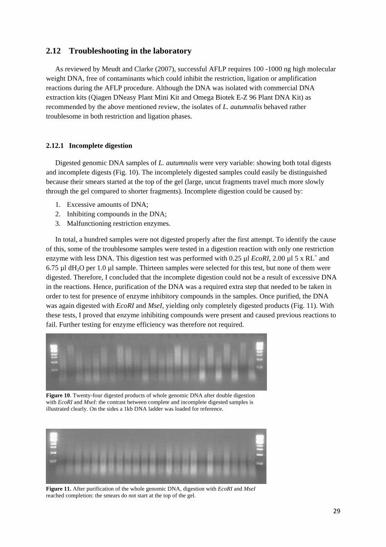
Digested genomic DNA samples of L. autumnalis were very variable: showing both total digests and incomplete digests (Fig. 10). The incompletely digested samples could easily be distinguished because their smears started at the top of the gel (large, uncut fragments travel much more slowly through the gel compared to shorter fragments). Incomplete digestion could be caused by:

1. Excessive amounts of DNA; 2. Inhibiting compounds in the DNA; 3. Malfunctioning restriction enzymes.

In total, a hundred samples were not digested properly after the first attempt. To identify the cause of this, some of the troublesome samples were tested in a digestion reaction with only one restriction enzyme with less DNA. This digestion test was performed with 0.25 µl EcoRI, 2.00 µl 5 x RL+ and 6.75 µl dH2O per 1.0 µl sample. Thirteen samples were selected for this test, but none of them were digested. Therefore, I concluded that the incomplete digestion could not be a result of excessive DNA in the reactions. Hence, purification of the DNA was a required extra step that needed to be taken in order to test for presence of enzyme inhibitory compounds in the samples. Once purified, the DNA was again digested with EcoRI and MseI, yielding only completely digested products (Fig. 11). With these tests, I proved that enzyme inhibiting compounds were present and caused previous reactions to fail. Further testing for enzyme efficiency was therefore not required.

 Figure 10. Twenty-four digested products of whole genomic DNA after double digestion with EcoRI and MseI: the contrast between complete and incomplete digested samples is illustrated clearly. On the sides a 1kb DNA ladder was loaded for reference.

 

 Figure 11. After purification of the whole genomic DNA, digestion with EcoRI and MseI reached completion: the smears do not start at the top of the gel.

29  

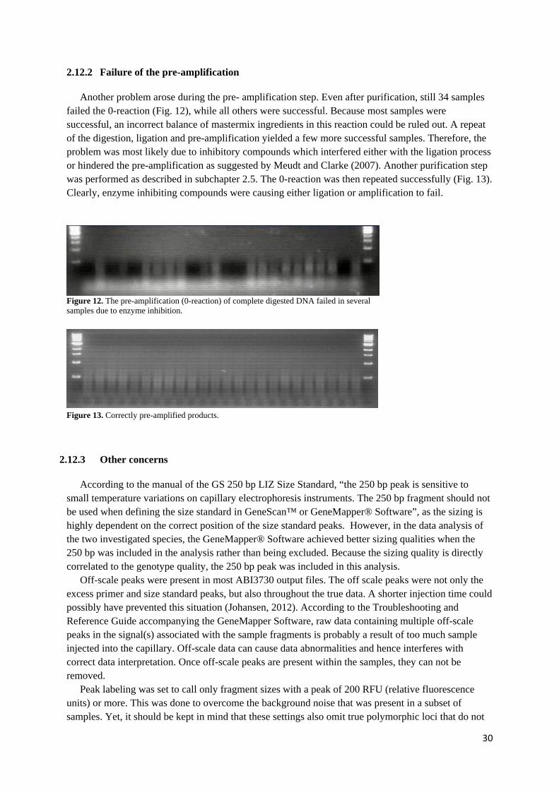
2.12.2 Failure of the pre-amplification

Another problem arose during the pre- amplification step. Even after purification, still 34 samples failed the 0-reaction (Fig. 12), while all others were successful. Because most samples were successful, an incorrect balance of mastermix ingredients in this reaction could be ruled out. A repeat of the digestion, ligation and pre-amplification yielded a few more successful samples. Therefore, the problem was most likely due to inhibitory compounds which interfered either with the ligation process or hindered the pre-amplification as suggested by Meudt and Clarke (2007). Another purification step was performed as described in subchapter 2.5. The 0-reaction was then repeated successfully (Fig. 13). Clearly, enzyme inhibiting compounds were causing either ligation or amplification to fail.

 Figure 12. The pre-amplification (0-reaction) of complete digested DNA failed in several samples due to enzyme inhibition.

 Figure 13. Correctly pre-amplified products.

 

2.12.3 Other concerns

According to the manual of the GS 250 bp LIZ Size Standard, “the 250 bp peak is sensitive to small temperature variations on capillary electrophoresis instruments. The 250 bp fragment should not be used when defining the size standard in GeneScan™ or GeneMapper® Software”, as the sizing is highly dependent on the correct position of the size standard peaks. However, in the data analysis of the two investigated species, the GeneMapper® Software achieved better sizing qualities when the 250 bp was included in the analysis rather than being excluded. Because the sizing quality is directly correlated to the genotype quality, the 250 bp peak was included in this analysis.

Off-scale peaks were present in most ABI3730 output files. The off scale peaks were not only the excess primer and size standard peaks, but also throughout the true data. A shorter injection time could possibly have prevented this situation (Johansen, 2012). According to the Troubleshooting and Reference Guide accompanying the GeneMapper Software, raw data containing multiple off-scale peaks in the signal(s) associated with the sample fragments is probably a result of too much sample injected into the capillary. Off-scale data can cause data abnormalities and hence interferes with correct data interpretation. Once off-scale peaks are present within the samples, they can not be removed.

Peak labeling was set to call only fragment sizes with a peak of 200 RFU (relative fluorescence units) or more. This was done to overcome the background noise that was present in a subset of samples. Yet, it should be kept in mind that these settings also omit true polymorphic loci that do not

30  

reach the 200 RFU threshold. Therefore, individual AFLP profiles that were having a lower RFU average (e.g. due to less amplified product passing through the capillary) could be miscalled, i.e. the fragments will not be detected and subsequently are scored as absent even if they are present.

Peak detection settings were optimized by repeating the analysis with different parameters. Further improvement could possibly have been reached by exploiting a combination of three softwares, GeneScanner, OptiFLP and TinyFLP to find the best peak detection settings for each data set (Arthofer et al., 2011). 

31  

 

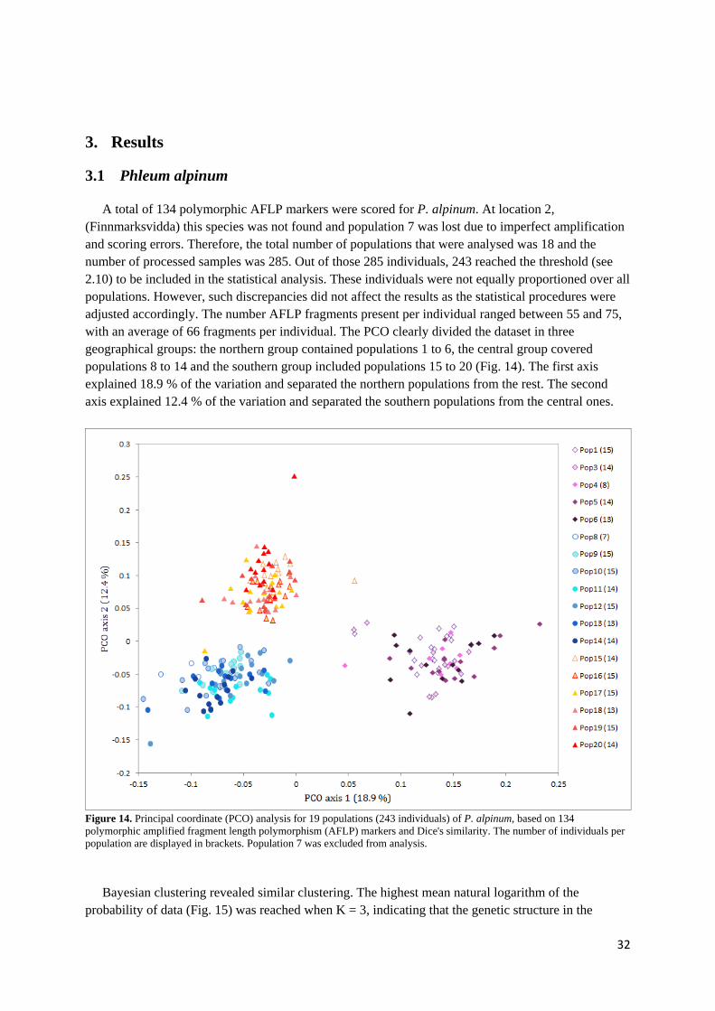
3. Results

3.1 Phleum alpinum

A total of 134 polymorphic AFLP markers were scored for P. alpinum. At location 2, (Finnmarksvidda) this species was not found and population 7 was lost due to imperfect amplification and scoring errors. Therefore, the total number of populations that were analysed was 18 and the number of processed samples was 285. Out of those 285 individuals, 243 reached the threshold (see 2.10) to be included in the statistical analysis. These individuals were not equally proportioned over all populations. However, such discrepancies did not affect the results as the statistical procedures were adjusted accordingly. The number AFLP fragments present per individual ranged between 55 and 75, with an average of 66 fragments per individual. The PCO clearly divided the dataset in three geographical groups: the northern group contained populations 1 to 6, the central group covered populations 8 to 14 and the southern group included populations 15 to 20 (Fig. 14). The first axis explained 18.9 % of the variation and separated the northern populations from the rest. The second axis explained 12.4 % of the variation and separated the southern populations from the central ones.

Figure 14. Principal coordinate (PCO) analysis for 19 populations (243 individuals) of P. alpinum, based on 134 polymorphic amplified fragment length polymorphism (AFLP) markers and Dice's similarity. The number of individuals per population are displayed in brackets. Population 7 was excluded from analysis.

Bayesian clustering revealed similar clustering. The highest mean natural logarithm of the

probability of data (Fig. 15) was reached when K = 3, indicating that the genetic structure in the

32  

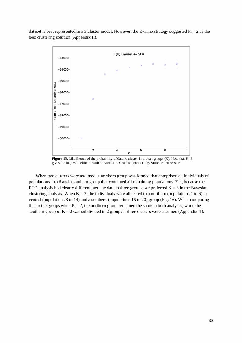
dataset is best represented in a 3 cluster model. However, the Evanno strategy suggested K = 2 as the best clustering solution (Appendix II).

 Figure 15. Likelihoods of the probability of data to cluster in pre-set groups (K). Note that K=3 gives the highestlikelihood with no variation. Graphic produced by Structure Harvester.

When two clusters were assumed, a northern group was formed that comprised all individuals of populations 1 to 6 and a southern group that contained all remaining populations. Yet, because the PCO analysis had clearly differentiated the data in three groups, we preferred K = 3 in the Bayesian clustering analysis. When K = 3, the individuals were allocated to a northern (populations 1 to 6), a central (populations 8 to 14) and a southern (populations 15 to 20) group (Fig. 16). When comparing this to the groups when K = 2, the northern group remained the same in both analyses, while the southern group of K = 2 was subdivided in 2 groups if three clusters were assumed (Appendix II).

33  

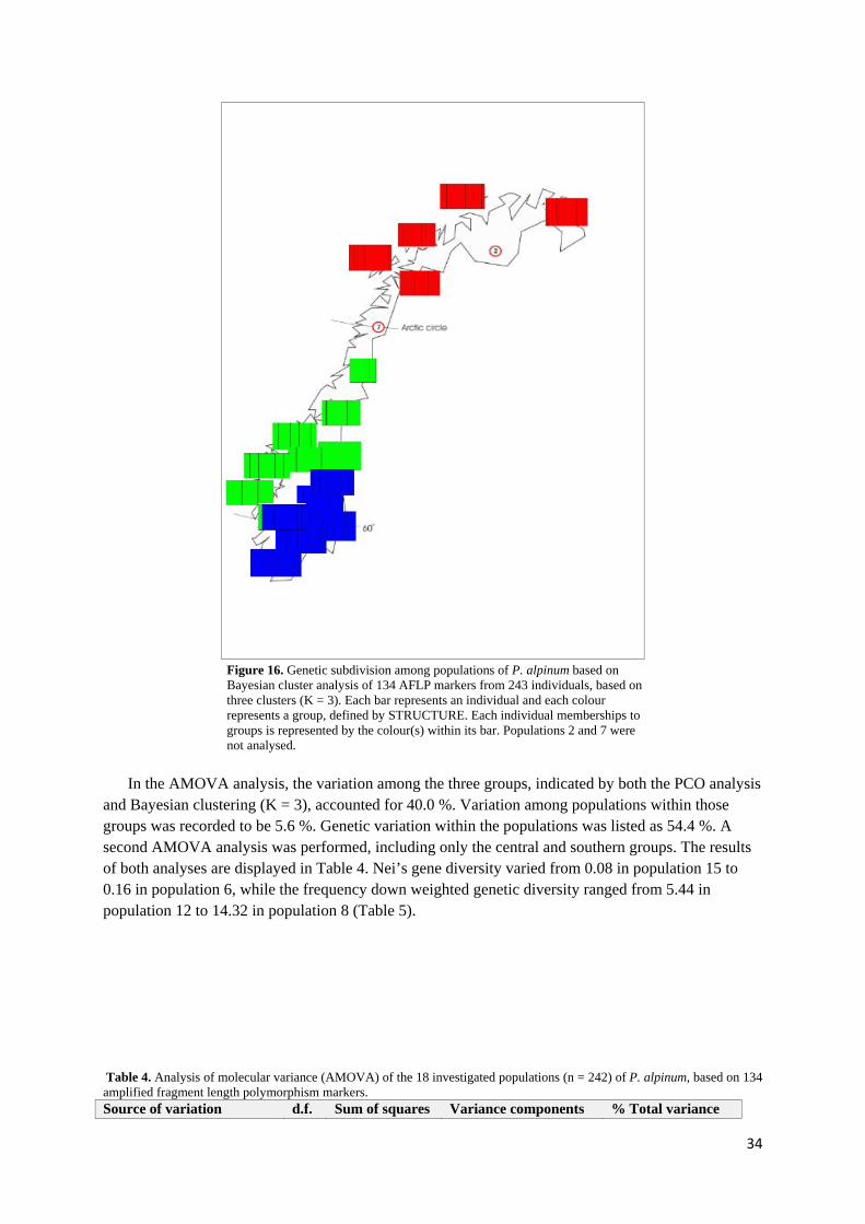
 Figure 16. Genetic subdivision among populations of P. alpinum based on Bayesian cluster analysis of 134 AFLP markers from 243 individuals, based on three clusters (K = 3). Each bar represents an individual and each colour represents a group, defined by STRUCTURE. Each individual memberships to groups is represented by the colour(s) within its bar. Populations 2 and 7 were not analysed.

In the AMOVA analysis, the variation among the three groups, indicated by both the PCO analysis

and Bayesian clustering (K = 3), accounted for 40.0 %. Variation among populations within those groups was recorded to be 5.6 %. Genetic variation within the populations was listed as 54.4 %. A second AMOVA analysis was performed, including only the central and southern groups. The results of both analyses are displayed in Table 4. Nei’s gene diversity varied from 0.08 in population 15 to 0.16 in population 6, while the frequency down weighted genetic diversity ranged from 5.44 in population 12 to 14.32 in population 8 (Table 5).

  

 

     Table 4. Analysis of molecular variance (AMOVA) of the 18 investigated populations (n = 242) of P. alpinum, based on 134 amplified fragment length polymorphism markers. Source of variation d.f. Sum of squares Variance components % Total variance

34  

AMOVA 1

Among groups (1-3) 2 1013.99 6.08 40.0

Among populations within groups 15 297.19 0.86 5.6 Within populations 225 1863.45 8.28 54.4

AMOVA 2

Among groups (1-2) 1 413.97 4.21 29.8

Among populations within groups 11 251.69 0.97 6.9

Within populations 173 1553.57 8.98 63.4

Table 5. The analysed population numbers, their locations, GPS coordinates, proportion of variable markers, Nei’s gene diversities (D) and Frequency down weighted gene diversities (DW) of the 18 investigated populations of P. alpinum. To adjust for unequal sample sizes, the proportion of variable markers and the genetic diversity measures (D and DW) were calculated with 7 randomly chosen individuals. This number was determined by the population with the fewest individuals included in all analyses. Population Location GPS

Coordinates (N/E)

Proportion of variable markers

D DW

1 Øst-Finnmark (Varanger) 70.23/29.40 0.25 0.10 10.54 3 Ytre Vestfinnmark/Magerøya 71.03/25.41 0.36 0.14 10.53 4 Lyngen 69.43/20.03 0.29 0.11 7.81 5 Lofoten/ (Kystfjella i Sør-Troms) 68.15/14.31 0.26 0.11 8.73 6 Ofoten/Bjørnefjell (Narvik) 68.26/17.25 0.40 0.16 9.46 8 Børgefjell 65.07/13.45 0.23 0.09 14.32 9 Meråker 63.23/43/27 0.28 0.11 6.90 10 Kvikne/Tynset (Rørosvidda) 62.34/10.17 0.30 0.13 7.87 11 Trollheimen 62.51/ 9.05 0.37 0.15 8.43 12 Dovrefjell 62.06/ 9.25 0.26 0.10 5.44 13 Strynefjellet 61.58/ 7.19 0.31 0.13 6.62 14 Vikafjellet 59.29/ 5.21 0.26 0.10 7.64 15 Valdresflya 61.23/ 8.48 0.20 0.08 7.01 16 Ringebufjellet 61.32/10.12 0.33 0.13 9.07 17 Hardangervidda vest/Ulvik/Finse 60.34/ 7.17 0.27 0.12 6.70 18 Hardangervidda øst/Rauland/Rjukan 59.53/ 8.29 0.32 0.15 9.91 19 Norefjell 60.13/ 9.33 0.37 0.15 8.63 20 Setesdal vesthei - Bykle/Valle/Sirdal 59.06/ 7.24 0.34 0.12 8.40

3.2 Leontodon autumnalis

Out of 300 plant samples, 42 individuals were culled from further analysis as they did not reach the threshold of 80 % of the average marker value. Due to this culling, only one individual of population 1 and two individuals of population 2 were left, while all other populations were represented with at least 11 individuals. Populations 1 and 2 were morphologically different from all other populations (Fig. 17), and their AFLP profiles differed as well. Therefore, populations 1 and 2 were suspected to be a different species and were dismissed from all analyses.

35  

                                   

                         A.                                                                            B. 

Figure 17. Populations from Varanger and Kautokeino possessed oval shaped leaves without lobes (A, picture obtained from http://www.glaucus.org.uk/Hawkbits.html), while the individuals from all other populations had mildly to sharply lobed leafs (B, (NatureGate 2012))

The analyses of L. autumnalis were performed using 150 polymorphic AFLP markers over 256 individuals belonging to 18 different populations. The average number of AFLP fragments present per individual was 65, with a range of 51 to 81 markers present per individual. The PCO analysis of this dataset did not reveal any true groupings, but did show some slight tendencies: northern group (population 3-6 appear mostly on the lower part axis 2, a central group (populations 10, 11 and 12 appear mostly on the left side on axis 1) and a southern group (populations 14, 15, 19 and 20 locate themselves predominantly on the right half of the axis 1, Fig. 18). The eigenvalues of the first two PCO axes accounted for 12.8 % of the variation within this alpine herb. When taking the first ten axes, 29 % of the variation was explained and half of all variation was captured by the first 25 axes.

36  

 Figure 18. Principal coordinates (PCO) analysis for 18 populations of L. autumnalis based on 150 polymorphic amplified fragment length polymorphism (AFLP) fragments and Dice's similarity. Numbers of individuals within a population are shown in brackets in the legend.

Exploiting the STRUCTURE software to infer molecular patterns of genetic similarity within the binary matrix gave conflicting results (Appendix III). The Evanno table suggested K = 2 as the best model, while the graph of the likelihood of the probability of data indicated that K = 3 is the preferable option. Results of K = 3 were transferred to the map to visualize potential genetic structuring (Fig. 19). The weak genetic structure obtained with the PCO could also vaguely be discovered in these results of STRUCTURE.

37  

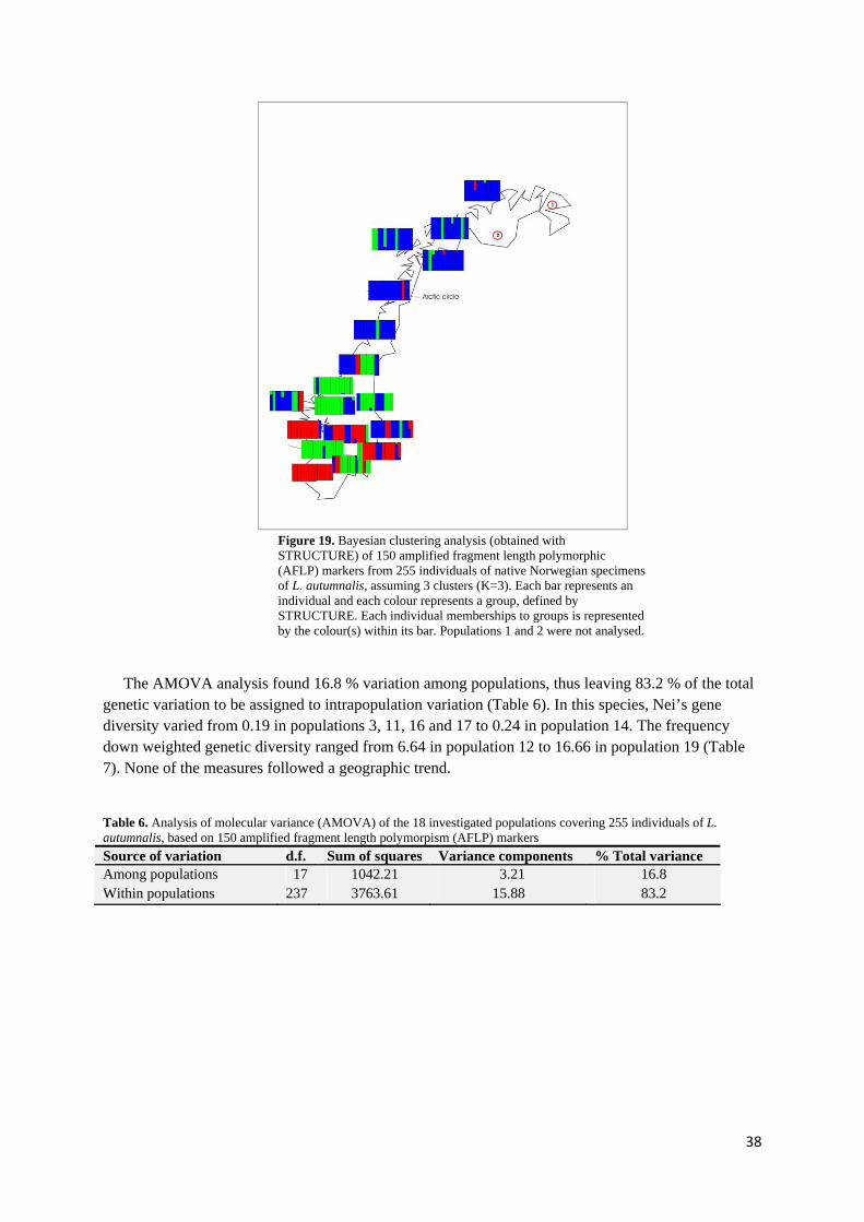
 Figure 19. Bayesian clustering analysis (obtained with STRUCTURE) of 150 amplified fragment length polymorphic (AFLP) markers from 255 individuals of native Norwegian specimens of L. autumnalis, assuming 3 clusters (K=3). Each bar represents an individual and each colour represents a group, defined by STRUCTURE. Each individual memberships to groups is represented by the colour(s) within its bar. Populations 1 and 2 were not analysed.

The AMOVA analysis found 16.8 % variation among populations, thus leaving 83.2 % of the total genetic variation to be assigned to intrapopulation variation (Table 6). In this species, Nei’s gene diversity varied from 0.19 in populations 3, 11, 16 and 17 to 0.24 in population 14. The frequency down weighted genetic diversity ranged from 6.64 in population 12 to 16.66 in population 19 (Table 7). None of the measures followed a geographic trend.

Table 6. Analysis of molecular variance (AMOVA) of the 18 investigated populations covering 255 individuals of L. autumnalis, based on 150 amplified fragment length polymorpism (AFLP) markers

Source of variation d.f. Sum of squares Variance components % Total variance Among populations 17 1042.21 3.21 16.8 Within populations 237 3763.61 15.88 83.2  

38  

 

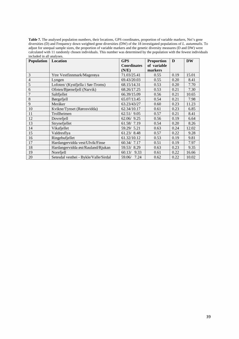
Table 7. The analysed population numbers, their locations, GPS coordinates, proportion of variable markers, Nei’s gene diversities (D) and Frequency down weighted gene diversities (DW) of the 18 investigated populations of L. autumnalis. To adjust for unequal sample sizes, the proportion of variable markers and the genetic diversity measures (D and DW) were calculated with 11 randomly chosen individuals. This number was determined by the population with the fewest individuals included in all analyses. Population Location GPS

Coordinates (N/E)

Proportion of variable markers

D DW

3 Ytre Vestfinnmark/Magerøya 71.03/25.41 0.55 0.19 15.01 4 Lyngen 69.43/20.03 0.55 0.20 8.41 5 Lofoten/ (Kystfjella i Sør-Troms) 68.15/14.31 0.53 0.20 7.70 6 Ofoten/Bjørnefjell (Narvik) 68.26/17.25 0.53 0.21 7.30 7 Saltfjellet 66.39/15.09 0.56 0.21 10.65 8 Børgefjell 65.07/13.45 0.54 0.21 7.98 9 Meråker 63.23/43/27 0.60 0.23 11.23 10 Kvikne/Tynset (Rørosvidda) 62.34/10.17 0.61 0.23 6.85 11 Trollheimen 62.51/ 9.05 0.57 0.21 8.41 12 Dovrefjell 62.06/ 9.25 0.56 0.19 6.64 13 Strynefjellet 61.58/ 7.19 0.54 0.20 8.26 14 Vikafjellet 59.29/ 5.21 0.63 0.24 12.02 15 Valdresflya 61.23/ 8.48 0.57 0.22 9.28 16 Ringebufjellet 61.32/10.12 0.53 0.19 9.81 17 Hardangervidda vest/Ulvik/Finse 60.34/ 7.17 0.51 0.19 7.97 18 Hardangervidda øst/Rauland/Rjukan 59.53/ 8.29 0.63 0.23 9.35 19 Norefjell 60.13/ 9.33 0.61 0.22 16.66 20 Setesdal vesthei - Bykle/Valle/Sirdal 59.06/ 7.24 0.62 0.22 10.02

 

 

 

 

 

 

39  

 

4. Discussion  

4.1 Genetic variation

Historical and contemporary events impact the genetic structuring of species mainly through gene flow, genetic drift and natural selection. Historical processes, such as glacial expansion and retreat, may have been inactive for hundreds of thousands of years, yet, their signatures will still be evident in the patterns of genetic diversity (Fjellheim et al., in prep.).

Glacial expansions and contractions repeatedly cause dramatic changes in species’ distributions. At the time of the last glacial period, migration into the Nordic area was not possible as the land was covered in ice sheets. When the ice melted, postglacial expansions were feasible because seeds and clones could establish themselves in the freshly deglaciated soils. Therefore, deglaciation patterns are directly related to the postglacial migration routes of plant species. After establishment of a species in such an area, the spatial genetic structuring of the species arises through the effectiveness of mating strategy, clonal growth, pollen distribution, seed dispersal and establishment, population density and isolation by distance (IBD). In the following subchapters, special genetic structure in Phleum alpinum and Leontodon autumnalis will be discussed in the light of these different processes.

4.1.1 Strong genetic structure in Phleum alpinum

The 18 Norwegian populations of the small perennial bunchgrass P. alpinum classified in three geographically coherent genetic groups (north, central and south, Fig.16). The genetic distinctiveness of these groups was high, and AMOVA assigned as much as 40.0 % of the genetic variation to the “among groups” section, while the populations within each group displayed extraordinary high similarity (only 5.6 % variation). From the Bayesian analysis of population structure, it became apparent that the central and southern groups are more closely related to eachother than they are to the northern group. It might be that these two groups represent descendants from two separate sources for post-glacial expansion. As illustrated in a review article by Hewitt (2000) the classical refugial areas are the Iberian peninsula, Italy and the Balkans (Fig. 20). Based on the findings of Fjellheim and Rognli (2005), it is suggested that both Festuca pratensis and Phleum pratense endured postglacial expansion via both western and eastern migration routes probably originating from the Iberian Peninsula and the Balkans, respectively, and similar migratory patterns may also be expected in P. alpinum. The southern and central genetic groups may have entered Norway through the southerly migratory pattern of the Iberian refugium, while the northern genetic cluster of P. alpinum is likely resulting from an expansion of a Baltic type that arrived in Norway through an easterly route. These are merely speculations, however, and it may be useful to exploit chloroplast DNA (cpDNA) markers to acquire more insight in the actual migratory patterns of P. alpinum.

40  

Figure 20. Map of Europe, showing the classical refugial areas Iberia (Ib), Italy (It) and the Balkans (Ba) in white circles, and cryptic refugia Hurd Deep (HD) and Carpathians (Ca) in yellow circles (Provan and Bennett 2008).

 

When the AMOVA was repeated for the two southern groups exclusively, the amount of variation among groups was 29.6 %, suggesting that barriers in gene flow have isolated these groups. This is even more plausible due to the fact that the variation among populations per group was as low as 6.9 %. It is likely that the suggested Iberian type has expanded throughout southern Norway and, over time, populations became separated into two genetically distinct groups due to lack of gene flow between the two groups, followed by random genetic drift and differences in selection pressures within the groups. The separation between the southern and the central group is in remarkably close concordance with the geographical distribution of the high mountain plateau and high glacial mountains of the Southern Scandes (Fig. 21) which includes Norway’s highest mountain Galhøppigen (2,469 m). The elevation and glaciation of these mountain ranges seem to have had a negative effect on gene flow between the populations on either side of this topographic barrier. A similar picture presents itself in the north, where the Saltfjellet-Svartisen National park arises to nearly 1600 meters above sea level, catering for Norway’s second largest glacier Svartisen. The delineation between the northern and central genetic groups of P. alpinum found in this study coincides with the geographical range of the mountain plateau. Hence, topographical relief and glaciation appear to be important factors in the organization of genetic structure within this alpine grass species.

In a study by Callaghan (1974), a comparison between populations from South Georgia and Disco Island (Greenland) was made regarding the species’ growth and reproductive strategy (Callaghan, 1974). This early work already revealed local adaptations, since the arctic populations demonstrated a high midseason growth spurt associated with favorable temperatures and notably elongated photoperiods, while the subantarctic populations exhibited a slower, but more linear growth pattern coinciding with the more balanced, but less favorable growing season. Reproduction differences were also concluded; the populations from Greenland were reaching much higher sexual reproductive capacity, but the short growth season rendered seed maturation to be limited. Therefore, actual seed output was low or zero in most years, but this was offset by the occasional high output when conditions allowed the seeds to reach maturity. On the contrary, the populations from South Georgia has a low but stable annual seed output (Callaghan, 1974). These results were later confirmed by

41  

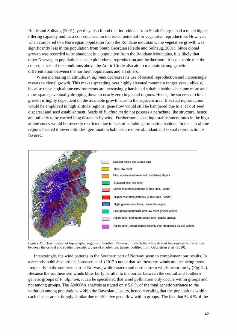
Heide and Solhaug (2001), yet they also found that individuals from South Georgia had a much higher tillering capacity and, as a consequence, an increased potential for vegetative reproduction. However, when compared to a Norwegian population from the Rondane mountains, the vegetative growth was significantly less in the population from South Georgian (Heide and Solhaug, 2001). Since clonal growth was recorded to be abundant in a population from the Rondane Mountains, it is likely that other Norwegian populations also exploit clonal reproduction and furthermore, it is plausible that the consequences of the conditions above the Arctic Circle also aid to maintain strong genetic differentiation between the northern populations and all others.

When increasing in altitude, P. alpinum decreases its use of sexual reproduction and increasingly reverts to clonal growth. This makes spreading over highly elevated mountain ranges very unlikely, because these high alpine environments are increasingly harsh and suitable habitats become more and more sparse, eventually dropping down to nearly zero in glacial regions. Hence, the success of clonal growth is highly dependent on the available growth sites in the adjacent area. If sexual reproduction would be employed in high altitude regions, gene flow would still be hampered due to a lack of seed dispersal and seed establishment. Seeds of P. alpinum do not possess a parachute like structure, hence are unlikely to be carried long distances by wind. Furthermore, seedling establishment rates in the high alpine zones would be severely restricted due to lack of suitable germination habitats. In the sub-alpine regions located it lower altitudes, germination habitats are more abundant and sexual reproduction is favored.

 Figure 21. Classification of topographic regions in Southern Norway, in which the white dashed line represents the border between the central and southern genetic groups of P. alpinum. Image modified from Gabrielsen et al. (2010).

Interestingly, the wind patterns in the Southern part of Norway seem to complement our results. In a recently published article, Jonassen et al. (2012 ) noted that southeastern winds are occurring most frequently in the southern part of Norway, while eastern and northeastern winds occur rarely (Fig. 22). Because the southeastern winds blow fairly parallel to the border between the central and southern genetic groups of P. alpinum, it can be speculated that wind pollination only occurs within groups and not among groups. The AMOVA analysis assigned only 5.6 % of the total genetic variance to the variation among populations within the Bayesian clusters, hence revealing that the populations within each cluster are strikingly similar due to effective gene flow within groups. The fact that 54.4 % of the

42  

total variation was assigned to the “within populations” section, meaning that the individual populations are diverse. This indicates that wind pollination is occurring in populations within groups.

All in all, the strong geographical genetic structure of P. alpinum in Norway is ideal for the production of site-specific seed, particularly because the three obtained groups are very conspicuous: each group is prominently different and the populations within each group are strikingly similar. In subchapter 4.2, these results are further explored in a more applied discussion regarding the actual use of our findings in the restoration context.

 Figure 22. Large scale wind distribution in Southwestern Norway (Jonassen, Ólafsson et al. 2012 )

4.1.2 Very weak of genetic structure in Leontodon autumnalis

In our investigation of 18 Norwegian populations of L. autumnalis, both the PCO and Bayesian clustering analysis were unable to detect a clear genetic structure. Although there were some elusive tendencies hinting towards two southern groups and a large northern group, the distinctness of these groups are questionable as the first two axes of the PCO analysis explained only 8.3 % and 4.5 % of the variation, respectively, and the between population variation in the entire dataset was only 16.8 % (Table 6). Besides, the STRUCTURE software gave also conflicting results regarding the best option for K. Therefore, it was difficult to determinate the best model. Although there was weak genetic structure in L. autumnalis, K = 1 was chosen as the best solution, due to the lack of prominence of the structuring. Therefore, Norway classifies as one homogenous zone. This result is congruent with the findings of Grass et al. (2006), who studied Central European populations of L. autumnalis. They found two groupings in their principal component analysis of 183 individuals based on 77 RAPD markers, corresponding to two chemotypes existing within the species. In Alpine regions only one of these particular chemotypes exists, hence it would not be surprising that the Norwegian populations in this study are actually one homogeneous group.

The weak spatial genetic structure can be explained in several ways. It is possible that there was only one introduction event after which the species experienced a large scale expansion, and another

43  

possibility is that the species of interest has very effective gene flow (Fjellheim et al., 2012). Further studies, e.g. cpDNA based marker studies, could be used to eliminate faulty options. Nevertheless when considering the biology of this alpine herb, a large amount of gene flow is a very plausible cause of the weak genetic structuring.

Seed and pollen movement are important factors that contribute largely to the gene flow and hence affect the genetic geographical structure. L. autumnalis is a very strategic heterocarpic outbreeding plant, using insect pollination combined with wind dispersal. Through the use of these strategies, both pollen and seed are carried over considerable distances. Pollination success in alpine environments depends largely on the amount of available pollinators in these regions and the effectiveness of the plant to attract these pollinators. Yellow flowers are preferred by many alpine pollinators (Kevan, 1972; McCall and Primack, 1992), hence the floral pigmentation of L. autumnalis is a definite advantage and enables the plant to maximize its gene flow associated with pollination. In the lower to medium alpine zone, pollinators are abundant and the population density of L. autumnalis is reasonably high, consequently leading to prominent gene flow. However, increasing altitude coincides with a reduction of pollinators (Sieber et al., 2011), therefore it can be speculated that pollination is less effective at high elevations. Nevertheless, this lack of pollination-attributed gene flow is likely compensated by an increased effectiveness of seed dispersal at such altitudes, as those regions are associated with particular strong winds. The development of feathery bristles (Fig. 10) on the achenes of L. autumnalis (Pico and Koubek, 2003) have a parachute-like function and allow the fruit bodies to be carried considerable distances by wind. Although south western winds predominate, the peaks of the mountains will allow turbulence to develop, probably assisting the achenes with well-developed plumage to be carried over mountain tops. Hence, this alpine plant also maximizes its seed dispersal mediated gene flow. Heterocarpy is enhancing the reproductive success of the alpine herb and, as a result, also contributes to the effectiveness of the species’ gene flow. The differences in morphology of the peripheral and central achenes drastically increase the potential of at least a subset of fruiting bodies to germinate, even when conditions at time of dispersal are far from ideal (Pico and Koubek, 2003).

4.2 Seed mixtures

Ecological restoration in the Norwegian mountain areas will benefit from the use of locally sourced seeds, as they are better adapted to survive in that specific habitat compared to seeds from other geographic origins. Unfortunately, it is hard to know exactly what a “local plant” is because it can be argued as a matter of “close proximity” (Lesica and Allendorf, 1999) or as a matter of “similar environment” (Montalvo and Ellstrand, 2000). In order to maximize the restoration potential of seed mixtures, it is important to gain knowledge regarding genetic diversity within species and its geographical genetic structure (McKay et al., 2005). Seed transfer zones should be delineated both with regards to the ability of the seeds to complete full life cycles as well as to decrease the risk of genetic pollution.

In general, the organization of genetic variation within populations is a dynamic process, influenced by the mating strategy, seedling germination efficiency, distribution density and whether or not the species is a long-lived perennial. High genetic diversity levels within populations are associated with an increased potential to adapt to changes (Wilkinson, 2001). Hence, in the context of restoration of disturbed mountain areas, genetic variation within populations should be investigated in order to identify optimal source populations for site-specific seed mixtures: populations with the highest genetic diversity will be the most suitable candidates due to their adaptive potential. In species

44  

with low genetic diversity within populations, genetically diverse seed mixtures may be obtained by mixing source populations within a genetically distinct zone.

In this study, we used AFLP markers to infer genetic structure and reveal zones of genetic distinctiveness as a guide to delineate seed transfer zones within Norway for P. alpinum and L. autumnalis and to discuss the implications of the findings in terms of commercial seed production for these species. Although both plants are distributed throughout most parts of Norway, samples were taken from 20 locations evenly distributed over Norway’s mainland. Twenty locations were chosen, based on the assumption that any genetic structuring would be captured by such a number of localities. More sampling localities would not fit within the capacity of this study.

The spatial genetic structure (SGS) derived from scanning a species with neutral markers, such as AFLPs, is meant to give seed growers, ecologists and plant physiologists a framework for the development of site-specific seedmixtures. One should note, however, that neutral genetic variation does not necessarily reflect adaptation. Neutral markers are by definition not affected by selection pressures and consequently are not capable of capturing adapted genetic variation. Hence, the classification of seed transfer zones is depending on neutral genetic markers in order to find structuring of genetic relatedness, but adaptations within a genetically related group could require further sub-structuring. Such refinement of the seed transfer zones can be achieved by controlled screening experiments that record seedling viability and phenotypic trait variability in different environmental conditions. In our case, this work will be undertaken as part of the ECONADA project, specifically work-package 4 (Appendix IV).

For restoration purposes, the exploited seeds should be genetically diverse in order to increase potential for sustainability of the vegetation resulting from that particular restoration project. We applied gene diversity measurements as a help for identifying the most diverse populations (Nei’s gene diversity) and populations with the most alleles (frequency down weighted gene diversity). Per genetically distinct group, the populations with the highest Nei’s diversity scores should be considered as optimal source candidates for commercial seed production. The frequency down weighted gene diversity measurement may be beneficial to identify populations containing the most alleles as a proportion of the total number of alleles in the dataset. Such an approach might be particularly useful in inbreeding species with short life cycles, as they are more vulnerable for isolation by distance and are less genetically diverse (Smith et al., 2009). Deliberate introduction of material sourced from allele-rich populations could increase the potential for adaptability to changing conditions (Kaye, 2001). Although gene diversity measures have great potential, one should be cautious when interpreting these values. In a review of statistical analysis methods for AFLP data, attention is drawn to two criteria which must be met for Nei’s gene diversity measures to be reliable. More precisely, the dataset should include information of at least several hundreds of loci and the species of interest must be outcrossing (Bonin et al., 2007). In this study, the first criterion has been violated, because the datasets were comprised of fewer loci. To maximize the chance of finding the most diverse source populations for seed production, the calculations could be repeated with more elaborate datasets. However, current results are used in this discussion.

4.2.1 Seed transfer zones and optimal source populations for Phleum alpinum

The results suggest that Norway encompasses three genetically distinct zones for P. alpinum (Fig.23), based on the PCO, STRUCTURE and AMOVA analyses. The northern zone includes Finnmark, Troms and the northern part of Nordland, the central zone consists of the remaining part of Nordland, Nord-Trøndelag, Møre og Romsdal, Sør-Trøndelag, Sogne og Fjordane and the northern regions of Hordaland, Oppland and Hedmark. The third phytogeographical zone for P. alpinum covers

45  

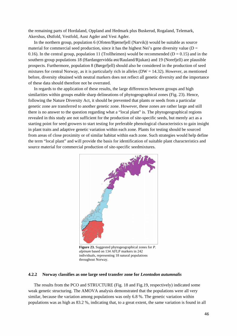
the remaining parts of Hordaland, Oppland and Hedmark plus Buskerud, Rogaland, Telemark, Akershus, Østfold, Vestfold, Aust Agder and Vest Agder.

In the northern group, population 6 (Ofoten/Bjørnefjell (Narvik)) would be suitable as source material for commercial seed production, since it has the highest Nei’s gene diversity value (D = 0.16). In the central group, population 11 (Trollheimen) would be recommended (D = 0.15) and in the southern group populations 18 (Hardangervidda øst/Rauland/Rjukan) and 19 (Norefjell) are plausible prospects. Furthermore, population 8 (Børgefjell) should also be considered in the production of seed mixtures for central Norway, as it is particularly rich in alleles (DW = 14.32). However, as mentioned before, diversity obtained with neutral markers does not reflect all genetic diversity and the importance of these data should therefore not be overrated.

In regards to the application of these results, the large differences between groups and high similarities within groups enable sharp delineations of phytogeographical zones (Fig. 23). Hence, following the Nature Diversity Act, it should be prevented that plants or seeds from a particular genetic zone are transferred to another genetic zone. However, these zones are rather large and still there is no answer to the question regarding what a “local plant” is. The phytogeographical regions revealed in this study are not sufficient for the production of site-specific seeds, but merely act as a starting point for seed growers to start testing for preferable phenological characteristics to gain insight in plant traits and adaptive genetic variation within each zone. Plants for testing should be sourced from areas of close proximity or of similar habitat within each zone. Such strategies would help define the term “local plant” and will provide the basis for identification of suitable plant characteristics and source material for commercial production of site-specific seedmixtures.

 Figure 23. Suggested phytogeographical zones for P. alpinum based on 134 AFLP markers in 242 individuals, representing 18 natural populations throughout Norway.

 

4.2.2 Norway classifies as one large seed transfer zone for Leontodon autumnalis

The results from the PCO and STRUCTURE (Fig. 18 and Fig.19, respectively) indicated some weak genetic structuring. The AMOVA analysis demonstrated that the populations were all very similar, because the variation among populations was only 6.8 %. The genetic variation within populations was as high as 83.2 %, indicating that, to a great extent, the same variation is found in all

46  

populations. Hence, based on the results of our AFLP analysis of L. autumnalis, it is suggested to treat the whole country as one seed transfer zone (Fig. 24).

To optimize the genetic potential of seed mixtures, populations with the highest Nei’s gene diversity scores, such as population 14 (D = 0.24) located in Valdresflya would be preferred. Yet, tests of phenotypic and adaptive variation should be performed and their outcomes may outweigh gene diversity rankings, especially if important phenotypic traits for seedling establishment are more prominent in other locations. However, it is unlikely that large differences in populations exist, because the AFLP data in this study revealed that the populations are genetically very similar.

In terms of the usefulness of this information for the production of site-specific seed mixtures, seed growers and all others involved can regard Norway as a genetic homogenous zone for L. autumnalis. The risk of genetic pollution is therefore minimal, as long as native Norwegian seeds are used in the restoration projects. Therefore, the focus can be completely on identification of local adaptations and suitable phenotypic characteristics.

 Figure 24. Suggested phytogeographical zone for L. autumnalis based on 150 AFLP markers in 255 individuals, representing 18 natural populations throughout Norway: the entire country is suggested as one zone (indicated in yellow).

 

 

4.3 Practical application of phytogeographical zonation in terms of restoration efforts

To elucidate the meaning of all our findings, a strictly hypothetical scenario will be presented in which seed mixtures for ecological restoration in mountain areas only contain seeds of P. alpinum and L. autumnalis. For each individual species, the phytogeographical zones have been revealed with our AFLP investigation. Within these zones, individuals are further tested for phenotypic qualities important for commercial production and successful restoration. These tests will also provide insight in local adaptations and resulting microhabitat requirements, thus giving a clue about what should be considered a local plant. In P. alpinum, such test should be performed in each of the three phytogeographical zones, possibly revealing that the plants located at highest altitudes or above the Arctic Circle are adapted to their local environments. For L. autumnalis, such tests also need to be

47  

performed in its large phytogeographical zone that encaptures all of the Norwegian mainland and, for example, may find that plants from a sheltered microhabitat are different from those who were sourced in windy conditions. Such insights would be recorded and the phytogeographical zones would be further structured into smaller zones that define what “local plants” are for each particular species.

Once all the required information has been gathered, the information of all species that must be included in the seedmixture is combined. In this case, the data of P. alpinum must be overlayed with the data of L. autumnalis (Fig. 25). In this simplistic model, the three geographical zones of P. alpinum (left) are overlaid with the one phytogeographical zone of L. autumnalis (center), and the resulting map (right) shows the different seed mixtures when no local adaptations had been found. In such case, only three different seed mixtures would be needed. However, adaptations are likely and therefore, it is expected that several seedmixtures are necessary per genetically distinct region.

To maximize restoration success, genetically diverse hotspots within each site-specific zone should be identified and utilized as source material for the subsequent seed mixtures. When possible, source material should be taken from areas where both species have high gene diversity scores. In the north, the preferred location would be Ofoten, while Trollheimen and Hardangervidda øst would be the locations of choice in the central and southern phytogeographical zones, respectively. Nevertheless, it is recommended to always prioritize site-specificity over diversity level.

 Figure 25. Simplified model that demonstrates the basis for site-specific seed mixtures: If site-specific seed mixtures were to contain only P. alpinum and L. autumnalis, then three mixtures should be produced based on the three phytogeograpical regions of P. alpinum (right), combined with the one of L. autumnalis (centre). The map on left results from overlapping the other two; the colours are mixed reflecting the inclusion of both species in the three seed mixtures. More seedmixtures are necessary when local ecotypes are identified.

48  

 

4.4 Validity concerns

As reviewed by Bonin et al (2007), experimental design is of utmost importance in AFLP studies. A minimum amount of 30 individuals per population was suggested in this review, to ensure accuracy. The number of markers should also be carefully considered, but the optimum number is difficult to address due to differences in species and their associate traits. Scoring of AFLP data can be difficult and subjective, especially in the presence of off-scale peaks and when differences in signal intensity between individuals or runs exist. Replicate runs of at least 5 – 10 % of the total numbers of samples are essential in order to estimate the error rate accurately.

The experimental design in this study failed to meet the recommendations suggested in the review, and the scoring of the data was hampered by both off-scale peaks and signal intensity differences. No replicates were included in this study, which severely limits the amount of conclusions based on this work. Yet, despite all discrepancies, the work was a first attempt to use AFLP marker technology in both P. alpinum and L. autumnalis and the results seem very plausible. When these results are being exploited in terms of their practical application in the ECONADA project, a sufficient amount of replicate runs will be included.

49  

 

5. Conclusions

Before this study, there was no existing knowledge about the genetic structuring in the alpine plants P. alpinum and L. autumnalis in Norway’s mainland. Through the use of the AFLP marker system, insights in the genetic structuring of these species have been gained, which allows for the establishment of a framework in which site-specific seed mixtures can be produced. By identifying seed transfer zones for both of the investigated species, this study has contributed essential knowledge necessary for the success of restoration projects in disturbed mountainous areas. Besides, it also enables the actual application of the Nature Diversity Act for these species.

Future work in this area should focus on the delineation of phytogeographical zones for more common alpine plant species, and identification of important seed establishment properties plus their expression requirements may refine these zones further in site-specific regions. Furthermore, efficient seed production strategies need to be developed and regulations should be proposed to launch the production of site-specific seed as a new business activity in Norway. Field trials in different ecological settings could provide more insight in delineating in which scenario ecological restoration through site-specific seed mixtures is beneficial and in which circumstances failure can be expected. Hence, such experiments are also recommended.

50  

Reference list  

Aamlid, T. S. 2011. Seed production of local populations for ecological restoration in Norwegian mountain areas. International Herbage Seed Group Newsletter. 45: 6-9. Afonin, A. N., Greene, S. L., Dzyubenko, N. I. and Frolov A. N. (eds.). 2008. Interactive agricultural ecological atlas of Russia and neighboring countries. Economic plants and their diseases, Pests and Weeds[Online]. Available at: http://www.agroatlas.ru. Andel, Van J. and Aronson, J. (eds.). 2012. Restoration ecology: The new frontier. Wiley-Blackwell, Chichester, UK. Second edition, 400pp.

Anderson, C. D., Epperson, B. K., Fortin, M. J., Holderegger, R., James P. M. A., Rosenberg, M. S., Scribner, K. T. and Spear S. 2010. Considering spatial and temporal scale in landscape-genetic studies of gene flow. Molecular Ecology. 19 (17): 3565-3575.

Arthofer, W., Schlick-Steiner, B. C. and Steiner, F. M. 2011. optiFLP: Software for automated optimization of amplified fragment length polymorphism scoring parameters. Molecular Ecology Resources. 11 (6): 1113-1118.

Bonin, A., Ehrich, D. and Manel, S. 2007. Statistical analysis of amplified fragment length polymorphism data: a toolbox for molecular ecologists and evolutionists. Molecular Ecology. 16 (18): 3737-3758. Caballero, A. and Quesada, H. 2010. Homoplasy and distribution of AFLP fragments: An analysis in silico of the genome of different species. Molecular Biology and Evolution. 27 (5): 1139-1151. Callaghan, T. V. 1974. Intraspecific variation in Phleum alpinum L. with specific reference to polar populations. Arctic and Alpine Research. 6 (4): 361-401. Chial, H. 2008. DNA fingerprinting using amplified fragment length polymorphisms (AFLP): No genome sequence required. Nature Education. 1 (1). Available at: http://www.nature.com Corander, J., Marttinen, P., Siren, J. and Tang, J. 2008. Enhanced bayesian modelling in BAPS software for learning genetic structures of populations. Bmc Bioinformatics. 9: 539. European Environment Agency 2005. Biogeographical regions: Available at: http://www.eea.europa.eu/data-and-maps/figures/biogeographical-regions-europe-2005-with-national-boundaries/biogeographical-regions_updated_colour_codes.

Earl, D. and Von Holdt, B. 2012. Structure Harvester: A website and program for visualizing STRUCTURE output and implementing the Evanno method. Conservation Genetics Resources. 4 (2): 359-361. Ehrich, D. 2006. AFLPdat: a collection of R functions for convenient handling of AFLP data. Molecular Ecology Notes. 6: 603-604.

51  

Elshire, R. J., Glaubitz, J. C., Sun, Q., Poland, J. A., Kawamoto, K., Buckler, E. S. and Mitchell, S. E. 2011. A robust, simple genotyping-by-sequencing (GBS) approach for high diversity species. Plos One. 6 (5): e19379. Elven, R., Murray, D. F., Razzhivin, V. Y. and Yurtsev, B. A. 2005. Annotated checklist of the panarctic flora (PAF) vascular plants. Available at http://nhm2.uio.no/paf/results?biogeographic=&bioclimatic=&region=&name=phleum#paf-344101 Excoffier, L. and Lischer, H. E. L. 2010. Arlequin suite ver 3.5: a new series of programs to perform population genetics analyses under Linux and Windows. Molecular Ecology Resources. 10 (3): 564-567. Excoffier, L., Smouse, P. E. and Quattro, J. M. 1992. Analysis of molecular variance inferred from metric distances among DNA haplotypes: Application to human mitochondrial DNA restriction data. Genetics. 131 (2): 479-91. Fjellheim, S. and Rognli, O. A. 2005. Molecular diversity of local Norwegian meadow fescue (Festuca pratensis Huds.) populations and Nordic cultivars-consequences for management and utilisation. Theoretical and Applied Genetics. 111 (4): 640-50. Fjellheim, S., Tanhuanpää, P., Marum, P., Manninen, O. & Rognli, O. Past and present population genetic processes in local populations of the cool season forage grass Phleum pratense- phylogeography, genetic structuring and local adaptation. In prep. Gabrielsen, R. H., Faleide, J. I., Pascal, C., Braathen, A., Nystuen, J. P., Etzelmuller, B. and O'Donnell, S. 2010. Latest caledonian to present tectonomorphological development of southern Norway. 27 (3): 709-723. Google Inc., 2012. Google Earth. Gort, G. and Van Eeuwijk, F. A. 2010. Codominant scoring of AFLP in association panels. Theoretical and Applied Genetics. 121 (2): 337-351. Government Administration Services 2009. Act of 19 June 2009 No. 100 Relating to the management of biological, geological and landscape diversity (Nature Diversity Act). Available at http://www.regjeringen.no Grass, S., Zidorn, C., Blattner, F. R. and Stuppner, H. 2006. Comparative molecular and phytochemical investigation of Leontodon autumnalis (Asteraceae, Lactuceae) populations from Central Europe. Phytochemistry. 67 (2): 122-31. Greuter, W., Gutermann, W. and Talavera, S. 2006. A preliminary conspectus of scorzoneroides (Compositae, Cichorieae) with validation of the required new names. Willdenowia. 36 (2): 689-692. Hammer, Ø., Harper, D. A. T. and Ryan, P. D. 2001. PAST: Paleontological Statistics Software Package for Education and Data Analysis. Palaeontologia Electronica, 4 (1): 9. Hamrick, J. L. and Nason, J. D. 1996. Consequences of dispersal in plants. In Rhodes, O. E., Chesser, R. K. and Smith, M. H. (eds.). Population dynamics in ecological space and time. University of Chicago Press, Chicago. 203-236. Heide, O. M. 1990. Dual floral induction requirements in Phleum alpinum. Annals of Botany. 66 (6): 687-694.

52  

Heide, O. M. and Solhaug, K. A. 2001. Growth and reproduction capacities of two bipolar Phleum alpinum populations from Norway and South Georgia. Arctic, Antarctic, and Alpine Research. 33 (2): 173-180. Hewitt, G. M. 2000. The genetic legacy of the Quarternary ice ages. Nature. 405 (6789): 907-913 Hultén, E. and Fries, M. 1986. Atlas of North European vascular plants: north of the Tropic of Cancer., vol. I-III. Königstein: Koeltz Scientific Books. Jensen, J., Bohonak, A. and Kelley, S. 2005. Isolation by distance, web service. BMC Genetics. 6 (1): 13. Johansen, M. 2012. Field Application Scientist dept. Nordic Technical Support of Life Technologies. Pers. communication Jombart, T., Pontier, D. and Dufour, A. B. 2009. Genetic markers in the playground of multivariate analysis. Heredity. 102 (4): 330-341. Jonassen, M., Ólafsson, H., Reuder, J. and Olseth, J. 2012. Multi-scale variability of winds in the complex topography of southwestern Norway. Tellus. A (64). Kaye, T. 2001. Common ground and controversy in native plant restoration: the SOMS debate, source distance, plant selections, and a restoration oriented definition of native. Native plant propagation and restoration strategies, Corvallis, Oregon: Nursery Technology Cooperative and Western Forestry and Conservation Association. 5-11 pp. Kevan, P. G. 1972. Insect pollination of high arctic flowers. Journal of Ecology. 60 (3): 831-847. Körner, C. 2003a. Mountain biodiversity: global hot spots, regional insurance, local lifelihood. Status and trends of, and threats to, mountain biodiversity, marine, coastal and inland water ecosystems: Abstracts of poster presentations at the eighth meeting of the subsidiary body on scientific, technical and technological advice of the convention on biological diversity, Montreal, Secretariat of the Convention on Biological Diversity. Körner, C. 2003b. Alpine plant life - functional plant ecology of high mountain ecosystems. Springer-Verlag, Berlin Heidelberg. Second edition, 344 pp. Krautzer, B., Graiss, W. and Poetsch, E. M. 2005. Evaluation of seed mixtures for subalpine pastures. Integrating Efficient Grassland Farming and Biodiversity. 10: 186-189. Krautzer, B., Kirmer, A., Haslgrübler, P. and Graiss, W. 2011. Seeds from semi-natural grassland as a source of biodiversity improvement. Available at: http://www.raumberg-gumpenstein.at Krautzer, B., Peratoner, G. and Bozzo, F. 2004. Site-specific grasses and herbs: Seed production and use for restoration of mountain environments. FAO plant production and protection series, vol. No. 32. Rome: Food and Agriculture Organization of the United Nations. vii, 111 s. pp. Latch, E., Dharmarajan, G., Glaubitz, J. and Rhodes, O. 2006. Relative performance of bayesian clustering software for inferring population substructure and individual assignment at low levels of population differentiation. Conservation Genetics, 7 (2): 295-302. Lesica, P. and Allendorf, F. W. 1999. Ecological genetics and the restoration of plant communities: Mix or match? Restoration Ecology. 7 (1): 42-50.

53  

Liu, Z. J. 2004. DNA marker technologies and their applications in aquaculture genetics. Aquaculture. 238: 1-37. Malaval, S., Lauga, B., Regnault-Roger, C. and Largier, G. 2010. Combined definition of seed transfer guidelines for ecological restoration in the French Pyrenees. Applied Vegetation Science. 13 (1): 113-124. McCall, C. and Primack, R. B. 1992. Influence of flower characteristics, weather, time of day, and season on insect visitation rates in three plant communities. American Journal of Botany. 79 (4): 434-442. McKay, J. K., Christian, C. E., Harrison, S. and Rice, K. J. 2005. "How local is local?" - A review of practical and conceptual issues in the genetics of restoration. Restoration Ecology. 13 (3): 432-440. Meudt, H. M. and Clarke, A. C. 2007. Almost forgotten or latest practice? AFLP applications, analyses and advances. Trends in Plant Science. 12 (3): 106-117. Mohamed-Yasseen, Y., Barringer, S., Splittstoesser, W. and Costanza, S. 1994. The role of seed coats in seed viability. The Botanical Review 60 (4): 426-439. Montalvo, A. M. and Ellstrand, N. C. 2000. Transplantation of the Subshrub Lotus scoparius: Testing the Home-Site Advantage Hypothesis. Conservation Biology. 14 (4): 1034-1045. Nason, J. D. and J. L. Hamrick 1997. Reproductive and genetic consequences of forest fragmentation: Two case studies of neotropical canopy trees. Journal of Heredity. 88(4): 264-276. NatureGate 2012. Autumn Hawkbit. Available at: http://www.luontoportti.com Nei, M. 1987. Molecular evolutionary genetics. Columbia University Press, New York. 512 pp. Nesje, A., Bakke, J., Dahl, S. O., Lie, O. and Matthews, J. A. 2008. Norwegian mountain glaciers in the past, present and future. Global and Planetary Change. 60 (1-2): 10-27. Nigel, G., Yoccoz, A. D. and Loison, A. 2010. Impact of climatic change on alpine ecosystems: inference and prediction. Revue de géographie alpine [Online], 98 (4). Norderhaug, A. and Sickel, H. 2007. A Norwegian summer farming landscape: a presentation of the characteristic summer farming landscape in south central Norway. In Europe's Living Landscapes: Essays Exploring our Identity in the Countryside, pp. 67-78. Zeist: KNNV Publishing. Picó, F. X. and Koubek, T. 2003. Inbreeding effects on fitness traits in the heterocarpic herb Leontodon autumnalis L. (Asteraceae). Acta Oecologica, 24 (5–6): 289-294. Primack, R. B. 2010. Essentials of conservation biology. 5 ed.: Sinauer Associates, Inc, Massachusetts. 601 pp. Pritchard, J. K., Stephens, M. and Donnelly, P. 2000. Inference of population structure using multilocus genotype data. Genetics. 155 (2): 945-959. Provan, J. and Bennett, K. D. 2008. Phylogeographic insights into cryptic glacial refugia. Trends in Ecology and Evolution. 23 (10): 564-571. Quinn, J. A. 2008. Arctic and Alpine biomes. Westport Greenwood Press, Connecticut. pp. 218. R Development Core Team, R. 2008. R: A language and environment for statistical computing. Foundation for Statistical Computing. Vienna, Austria. Available at: www.r-project.org

54  

Samuel, R., Gutermann, W., Stuessy, T. F., Ruas, C. F., Lack, H.-W., Tremetsberger, K., Talavera, S., Hermanowski, B. and Ehrendorfer, F. 2006. Molecular phylogenetics reveals Leontodon (Asteraceae, Lactuceae) to be diphyletic. American Journal of Botany. 93 (8): 1193-1205. Schönswetter, P. and Tribsch, A. 2005. Vicariance and dispersal in the alpine perennial Bupleurum stellatum L. (Apiaceae). Taxon. 54 (3): 725-732. Semagn, K., Bjornstad, A. and Ndjiondjop, M. N. 2006. An overview of molecular marker methods for plants. African Journal of Biotechnology. 5 (25): 2540-2568. Sieber, Y., Holderegger, R., Waser, N. M., Thomas, V. F. D., Braun, S., Erhardt, A., Reyer, H.-U. and Wirth, L. R. 2011. Do alpine plants facilitate each other’s pollination? Experiments at a small spatial scale. Acta Oecologica. 37 (4): 369-374. Smith, B. M., Diaz, A., Daniels, R., Winder, L. and Holland, J. M. 2009. Regional and Ecotype Traits in Lotus corniculatus L., with Reference to Restoration Ecology. Restoration Ecology, 17 (1): 12-23. Stewart, A. V., Joachimiak, A. J. and Ellison, N. W. 2009. Genomic and geographic origins of timothy (Phleum sp.) based on ITS and chloroplast sequences. Molecular Breeding of Forage and Turf. 71-81. Stewart, A. V., Joachimiak, A. J. and Ellison, N. W. 2011. Wild Crop Relatives: Genomic and Breeding Resources. C. Kole (ed.), Springer Berlin Heidelberg: 257-274. Storfer, A., Murphy, M. A., Spear, S. F., Holderegger, R. and Waits, L. P. 2010. Landscape genetics: where are we now? Molecular Ecology, 19 (17): 3496-3514. Tamegger, C. and Krautzer, B. 2006. Production and use of site specific seed in Austria. In, Irdning: HBLFA Raumberg-Gumpenstein. pp. 113-118. Toro, M. A. and Caballero, A. 2005. Characterization and conservation of genetic diversity in subdivided populations. Philosophical Transactions of the Royal Society B-Biological Sciences, 360 (1459): 1367-1378. Totland, O. 1993. Pollination in alpine Norway-Flowering phenology, insect visitors, and visitation rates in two plant communities. Canadian Journal of Botany-Revue Canadienne De Botanique. 71 (8): 1072-1079. Trapnell, D. W., Schmidt, J. P. and Hamrick, J. L. 2008. Spatial genetic structure of the Southeastern North American endemic, ceratiola ericoides (Empetraceae). Journal of Heredity. 99 (6): 604-609. Vos, P., Hogers, R., Bleeker, M., Reijans, M., Vandelee, T., Hornes, M., Frijters, A., Pot, J., Peleman, J., Kuiper, M., et al. 1995. Aflp - a New Technique for DNA-Fingerprinting. Nucleic Acids Research. 23 (21): 4407-4414. Wilkinson, D. M. 2001. Is local provenance important in habitat creation? Journal of Applied Ecology. 38 (6): 1371-1373. Yurukova-Grancharova, P. D. 2004. On the embryology of Leontodon autumnalis (Asteraceae) Phytologica Balcanica. 10 (1): 85-91.

55  

56  

Appendices  

 

 

 

 

 

 

 

 

 

 

 

 

 

 

 

 

 

 

 

 

 

 

 

 

57  

 

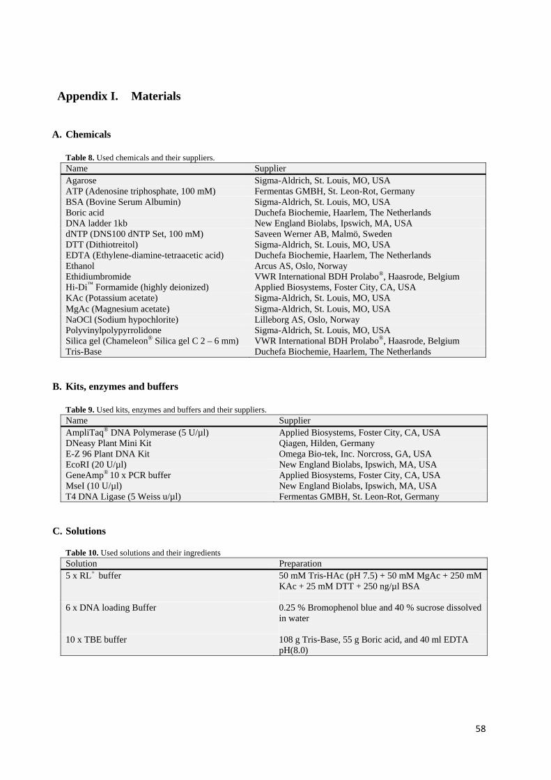
Appendix I. Materials  

A. Chemicals

Table 8. Used chemicals and their suppliers. Name Supplier Agarose Sigma-Aldrich, St. Louis, MO, USA ATP (Adenosine triphosphate, 100 mM) Fermentas GMBH, St. Leon-Rot, Germany BSA (Bovine Serum Albumin) Sigma-Aldrich, St. Louis, MO, USA Boric acid Duchefa Biochemie, Haarlem, The Netherlands DNA ladder 1kb New England Biolabs, Ipswich, MA, USA dNTP (DNS100 dNTP Set, 100 mM) Saveen Werner AB, Malmö, Sweden DTT (Dithiotreitol) Sigma-Aldrich, St. Louis, MO, USA EDTA (Ethylene-diamine-tetraacetic acid) Duchefa Biochemie, Haarlem, The Netherlands Ethanol Arcus AS, Oslo, Norway Ethidiumbromide VWR International BDH Prolabo®, Haasrode, Belgium Hi-Di™ Formamide (highly deionized) Applied Biosystems, Foster City, CA, USA KAc (Potassium acetate) Sigma-Aldrich, St. Louis, MO, USA MgAc (Magnesium acetate) Sigma-Aldrich, St. Louis, MO, USA NaOCl (Sodium hypochlorite) Lilleborg AS, Oslo, Norway Polyvinylpolypyrrolidone Sigma-Aldrich, St. Louis, MO, USA Silica gel (Chameleon® Silica gel C 2 – 6 mm) VWR International BDH Prolabo®, Haasrode, Belgium Tris-Base Duchefa Biochemie, Haarlem, The Netherlands

B. Kits, enzymes and buffers

Table 9. Used kits, enzymes and buffers and their suppliers. Name Supplier AmpliTaq® DNA Polymerase (5 U/µl) Applied Biosystems, Foster City, CA, USA DNeasy Plant Mini Kit Qiagen, Hilden, Germany E-Z 96 Plant DNA Kit Omega Bio-tek, Inc. Norcross, GA, USA EcoRI (20 U/µl) New England Biolabs, Ipswich, MA, USA GeneAmp® 10 x PCR buffer Applied Biosystems, Foster City, CA, USA MseI (10 U/µl) New England Biolabs, Ipswich, MA, USA T4 DNA Ligase (5 Weiss u/µl) Fermentas GMBH, St. Leon-Rot, Germany

C. Solutions Table 10. Used solutions and their ingredients Solution Preparation 5 x RL+ buffer 50 mM Tris-HAc (pH 7.5) + 50 mM MgAc + 250 mM

KAc + 25 mM DTT + 250 ng/µl BSA

6 x DNA loading Buffer 0.25 % Bromophenol blue and 40 % sucrose dissolved in water

10 x TBE buffer 108 g Tris-Base, 55 g Boric acid, and 40 ml EDTA pH(8.0)

58  

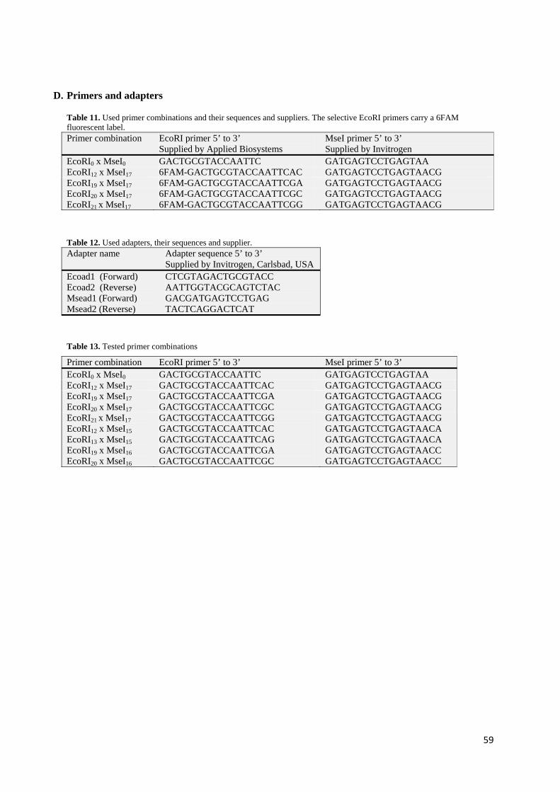
D. Primers and adapters Table 11. Used primer combinations and their sequences and suppliers. The selective EcoRI primers carry a 6FAM fluorescent label. Primer combination EcoRI primer 5’ to 3’

Supplied by Applied Biosystems MseI primer 5’ to 3’ Supplied by Invitrogen

EcoRI0 x MseI0 GACTGCGTACCAATTC GATGAGTCCTGAGTAA EcoRI12 x MseI17 6FAM-GACTGCGTACCAATTCAC GATGAGTCCTGAGTAACG EcoRI19 x MseI17 6FAM-GACTGCGTACCAATTCGA GATGAGTCCTGAGTAACG EcoRI20 x MseI17 6FAM-GACTGCGTACCAATTCGC GATGAGTCCTGAGTAACG EcoRI21 x MseI17 6FAM-GACTGCGTACCAATTCGG GATGAGTCCTGAGTAACG Table 12. Used adapters, their sequences and supplier. Adapter name Adapter sequence 5’ to 3’

Supplied by Invitrogen, Carlsbad, USA Ecoad1 (Forward) Ecoad2 (Reverse) Msead1 (Forward) Msead2 (Reverse)

CTCGTAGACTGCGTACC AATTGGTACGCAGTCTAC GACGATGAGTCCTGAG TACTCAGGACTCAT

 Table 13. Tested primer combinations

 Primer combination EcoRI primer 5’ to 3’ MseI primer 5’ to 3’ EcoRI0 x MseI0 GACTGCGTACCAATTC GATGAGTCCTGAGTAA EcoRI12 x MseI17 GACTGCGTACCAATTCAC GATGAGTCCTGAGTAACG EcoRI19 x MseI17 GACTGCGTACCAATTCGA GATGAGTCCTGAGTAACG EcoRI20 x MseI17 GACTGCGTACCAATTCGC GATGAGTCCTGAGTAACG EcoRI21 x MseI17 EcoRI12 x MseI15 EcoRI13 x MseI15 EcoRI19 x MseI16 EcoRI20 x MseI16

GACTGCGTACCAATTCGG GACTGCGTACCAATTCAC GACTGCGTACCAATTCAG GACTGCGTACCAATTCGA GACTGCGTACCAATTCGC

GATGAGTCCTGAGTAACG GATGAGTCCTGAGTAACA GATGAGTCCTGAGTAACA GATGAGTCCTGAGTAACC GATGAGTCCTGAGTAACC

 

 

 

 

 

59  

 

E. Laboratory equipment Table 14. List of all equipment and corresponding suppliers, sorted by function. Function Equipment Manufacturer Centrifugation 1. Eppendorf Centrifuge 5810R Eppendorf AG, Hamburg, Germany 2. Kendro Biofuge Pico Kendro Laboratory Products, Osterode, Germany 3. Sigma 4-16 Sigma Laborzentrifugen GmbH, Osterode, Germany Gel electrophoresis BioRad PowerPack 300 BioRad Laboratories, Hercules, CA, USA Gel imaging Gel Doc EQ Universal Hood II BioRad Laboratories, Segrate (Milan), Italy Homogenization 1. Retsch® MM301 Mixer Mill Retsch GmbH & Co., Haan, Germany 2. IKA® MS2 Minishaker

3. Tungsten Carbide beads (3 mm)

IKA Works, Inc., Wilmington, NC, USA Qiagen, Hilden, Germany

Incubation 1. Grant GD 120 waterbath Grant Instruments (Cambridge) Ltd., Shepreth, England

2. Grant OLS 200 waterbath 3. Parafilm

Grant Instruments (Cambridge) Ltd., Shepreth, England Pechiney Plastic Packaging Company, Chicago, IL, USA

PCR 1. C1000™ Thermal Cycler BioRad Laboratories, Hercules, CA, USA 2. GeneAmp® PCR System 9700 Applied Biosystems, Singapore, Singapore Weighing 1. Sartorius H51 balance Sartorius GmbH, Göttingen, Germany 2. Mettler AJ100L balance Mettler-Toledo AG, Greifensee, Switzerland  

F. Software

Table 15. Used software programs and packages with their sources or associated references. Software Sources Arlequin 3.5 (Excoffier and Lischer 2010) AFLPdat (Ehrich 2006) GeneMapper 4.1 Applied Biosystems, Foster City, CA USA PAST (Hammer, Harper et al. 2001) R 2.15.0 (R Development Core Team 2008) STRUCTURE 2.3.3 STRUCTURE Harvester 0.6.8

(Pritchard, Stephens et al. 2000) (Earl and vonHoldt 2012)

Quantity One 4.5.0 Biorad Laboratories, Hercules, CA, USA  

 

 

 

 

 

60  

 

Appendix II. STRUCTURE results for Phleum alpinum  

 

 

    

61  

 

K = 2 

 

K = 3 

62  

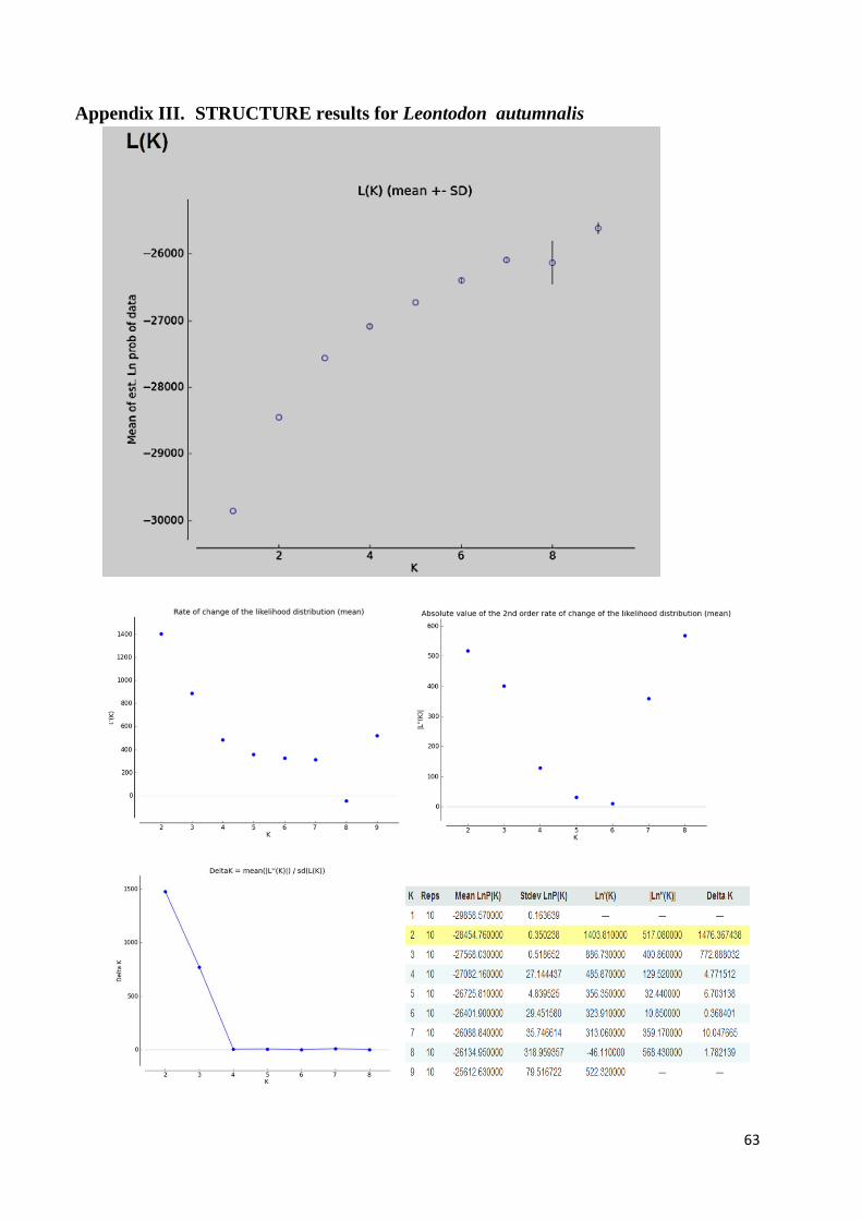
Appendix III. STRUCTURE results for Leontodon autumnalis

 

 

 

63  

 

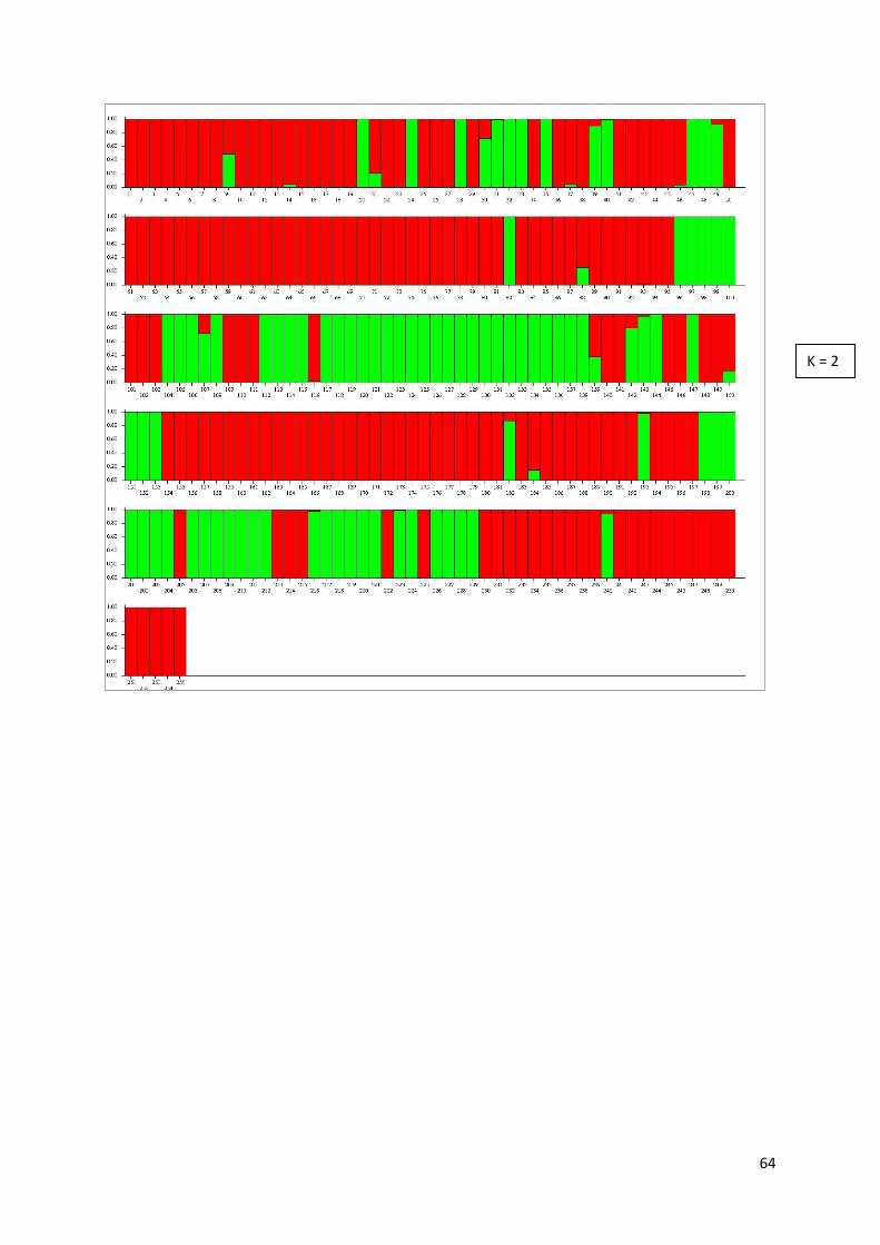
K = 2 

64  

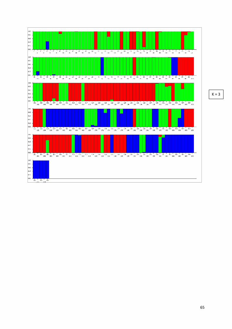
K = 3 

65  

 

 

Appendix IV. AMOVA results for Phleum alpinum

 

 

66  

 

Second AMOVA for P. alpinum: only the southern groups included

 

67  

 

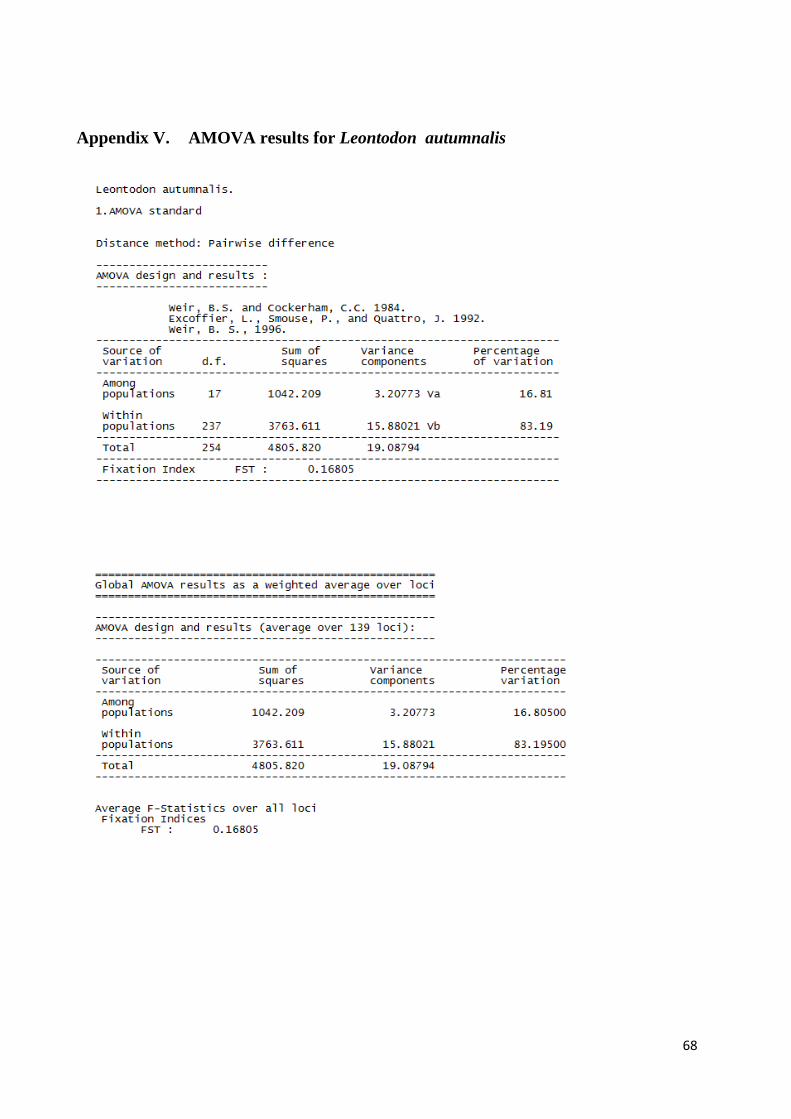
Appendix V. AMOVA results for Leontodon autumnalis  

 

 

 

 

68  

 

Appendix VI. Description of the ECONADA project

Objectives Principal objective Definition and provision of site-specific seed for ecological restoration, identification of criteria for successful establishment from seed, and clarification of impact of sowing on long-term ecological processes Subgoals 1. To define at least ten model species important for ecological restoration in Norway, and to identify suitable seed sources and collect seed ecotypes of these species 2. To delineate the term “site-specific seed” using DNA analyses, thus enabling a broad division of Norway into operational seed transfer zones for ecological restoration 3. To find optimal locations, develop efficient methods and identify appropriate regulations for seed multiplication, thus establishing production of site-specific seed as a new enterprise for Norwegian seed growers 4. To identify key traits for seedling establishment and how the expression of these traits varies among and within species and with environmental conditions to improve establishment success under both assisted and spontaneous restoration 5. To clarify the impact of ecological factors on seed establishment after various types of disturbances, and to determine when sowing is an appropriate measure and its implications for long term vegetation development for successful establishment from seed, and clarification of impact of sowing on long-term ecological processes

Frontiers of knowledge and technology Norway is committed to the conservation of biodiversity by international conventions. Major threats against biodiversity are natural interventions, loss of habitats and the introduction of nonadapted plant material. Ecological restoration strives to minimize negative impacts of disturbances, and to prevent dissemination of introduced species and ecotypes (Hagen & Skrindo 2010). Rapid establishment of vegetation following human-caused disturbance of landscape is often necessary to control erosion and for aesthetic reasons. Seeding of commercial grass species has been the traditional management strategy. However, if soil moisture or physical or chemical factors are not suitable, the sowing effort can fail (Heneghan et al. 2008). There is a need for more knowledge on when sowing is justified, and when it is unnecessary or even can have negative impact on vegetation dynamics (Rehounkova & Prach 2008, Tropek et al. 2010). The effects of sowing new species or ecotypes into local plant communities are often unpredictable and there is a concern that introduced material can displace original vegetation or breed with locally adapted ecotypes and reduce their fitness (Sackville Hamilton 2001, McKay et al 2005, Jones & Monaco 2009, van der Mijnsbrugge et al. 2009, Bischoff et al. in press). Seed collection and multiplication of site-specific ecotypes

69  

for restoration is not only ecologically sound, but it also opens new opportunities for local seed growers ( Krauzer et al. 2004; Aamlid 2008). Few studies have been undertaken to characterize genetic variation in plant species relevant for restoration purposes. Håbjørg (1979) found considerable genetic variation among ecotypes of Poa pratensis across Norway. More recently, altitudinal genetic differentiation was described in the alpine grasses Festuca eskia and Poa hiemata (Byars et al 2009, Gonzalo-Turpin & Hazard 2009). Complex distribution patterns of genetic variation were documented using molecular genetic markers in the outbreeding species Festuca pratensis (Fjellheim & Rognli 2005) and in the inbreeding weed Arabidopsis thaliana (Anna Lewandowska, submitted to Molecular Ecology). Molecular markers have also been used to define phytogeographical regions for ecological restoration in the French Pyrenees (Malaval et al. 2010). However, as neutral markers do not always coincide with quantitative traits important for restoration (Gebremedhin et al. 2009, (Kramer & Havens 2009), the use of such markers have to be accompanied by studies on local adaptation to maximize fitness of selected ecotypes.

Research tasks

On 19 June 2009, the Norwegian Parliament passed the new Nature Diversity Act (Naturmangfoldloven, Norwegian Government 2009). Chapter IV of this Act, which has not yet come into force, prohibits the release of „organisms belonging to species or subspecies that do not occur naturally in Norway, into the environment’ and ‘organisms that do not already occur naturally in an area into the environment if the King has made regulations

requiring a permit for this purpose.‟ (§30a & d). In its document “Intersectorial national

strategy and measures against alien, harmful species” the Norwegian Ministry of Environment (2007) defines “alien organisms” as “a species, subspecies or lower taxon, including population, which has been introduced outside its present or historical area of occurrence”. This document also mentions „production of site-specific seed mixtures and suitable plant material for vegetation establishment after natural inventions’ as an area of high priority.

There are four important scientific and practical challenges related to the implementation of the Nature Diversity Act that will be dealt with in this project: First, there is a need for scientific and practical definition of the terms “native” and “site-specific”. Although alternative approaches have been suggested (e.g. Broadhurst et al. 2008), restoration guidelines often operate with seed transfer zones that restrict the distances over which seeds can be used. The scale of local adaptation along environmental gradients varies with species, populations, and the degree of environmental heterogeneity (Antonovics 1976, Endler 1986, Jones & Monaco 2009) and it often makes it difficult to define seed transfer zones (van der Mijnsbrugge et al. 2009). To meet these difficulties, molecular genetic tools can be used for choosing appropriate local material, as recently shown by Malaval et al. (2010). Information about the scale of (molecular) genetic variation and population genetic structure in key species commonly found in Norwegian vegetation is necessary to create a first basis for division of Norway into phytogeographical regions for restoration, and it will provide guidelines by which ecotypes can be amalgamated for seed multiplication. Second, efficient

70  

seed propagation methods have to be developed. Expected problems associated with seed production of undomesticated species are slow establishment resulting in weed problems and contaminated seed lots, susceptibility to diseases, inadequate conditions for flower induction, uneven ripening and seed shattering, seed cleaning complications resulting from seed hulls or chaff, and seed germination issues (Krauzer et al. 2004, Aamlid et al. 2010a). Some of these problems may be resolved by choosing locations for seed production outside the lowland areas in eastern Norway that are presently producing seed of forage grasses (Aamlid 1990). Seed multiplication closer to the area of adaptation is likely to reduce the risk for loss of genetic diversity and selection for particular genotypes that can otherwise result from repeated propagation (van der Mijnsbrugge et al. 2009). Through the projects Hjerkinn-PRO (2006-2012) “Fjellfrø” (2007-2010) and “Nordfrø”(2008-2010), seed growers in Telemark and Finnmark have already started multiplying native seed of 5-6 species for restoration purposes, and these initiatives have to be coordinated and followed up by research into optimal seed crop management and productions sites. Seed quality issues also have to be resolved by national regulations and harmonization at the European level. Third, poor germination and seedling survival has limited restoration success in more than 50 % of restoration attempts in the Norwegian mountains during the past three decades (H. Østhagen NVE, personal comm.). As seedling mortality due to drought stress is a major constraint to plant establishment on disturbed sites (Bell & Bliss 1980, Chambers 1995), seedling traits governing drought avoidance, tolerance and recovery seems to be of special importance in combination with practical measures to improve establishment conditions. Adaptive phenotypic plasticity in water-use traits are well documented (Thomas et al 1996, Huang & Gao 2000, Hagen 2003), and this aspect warrants further investigation in an ecological restoration context (Nicotra & Davidson 2010). Fourth, we need more information about the ecological possibilities and constraints of using native seeds in restoration projects. Besides the the short-term challenge related to the establishment of vegetation under different environmental conditions, the long term effects on vegetation dynamics of using seed in biodiversity management has to be evaluated. The whole concept of “What is successful restoration?” is part of this evaluation (Hagen & Skrindo 2010b). In a management situation both scientific, social and technical criteria must be included (Hagen 2003) and ecological attributes must be developed (SER 2004). More knowledge is needed on successional dynamics of the vegetation following restoration, including effects of succession enhancing treatments.

Disturbed sites are often liable to erosion, and they differ from vegetated sites with respect to important ecological and microclimatic factors such as surface stability, nutrient availability, temperature, water regime, soil texture and organic matter content (Walker & del Moral 2003). There is a need to determine when seed availability is limiting to plant colonization (Cooper et al. 2004, Tormo et al. 2006) and in what situations sowing is a useful method for management of biodiversity and landscape. Studies have to be undertaken at roadsides, gravel pits, hydropower heaps etc., and the reference sites studied over many years (Ruiz-Jaen & Aide 2005).

71  

Research approach, methods

WP 1. Selection of model species and collection of plant material

Ten model species common to natural and semi-natural landscapes over most of the country and with qualities that makes them likely components in restoration seed mixtures will be selected. Seed and leaf material has already been collected of Festuca ovina. Other model species will be chosen from various plant families based on breeding system (outbreeding, inbreeding, apomictic etc.), life cycle (annual, biennial perennial), ecological preferences, vegetative versus reproductive propagation strategies and other ecological and practical criteria. Candidate species are Agrostis capillaris, Avenella flexuosa, Anthoxanthum odoratum, Festuca rubra, Poa alpina, Phleum alpinum, Luzula multiflora, Leodonton autumnalis, Achillea millefolium and Viccia cracca. The final decision about model species will be taken in winter /spring 2011. During the summer 2011, leaf material and seed from at least 20 local ecotypes of each species representing different geographical regions will be collected.

WP 2. Analyses of genetic diversity and definition of phytogeographical regions

The collected plant material will be analysed for Amplified Fragment Length Polymorphism (AFLP) variation (Vos et al. 1995). Analyses of genetic diversity will usually be based on 15 individual plants from each ecotype, but this number may vary depending on life history traits of the species in question. A set of PstI/MseI primer combinations will be tested for degree of polymorphism using a restricted number of individuals selected from diverse populations, and a few highly polymorphic primer combinations sufficient to generate about 100 AFLP marker loci will be applied to the complete set of genotypes. Prinicipal component analyses, clustering analyses and analyses of molecular variance (AMOVA) will provide a precise description of genetic diversity levels as well as genetic distribution patterns of the different species. The results will serve as a guideline for choosing ecotypes to be used for seed production (WP 3) and for splitting the country into seed transfer zones. Our hypothesis is that molecular genetic analyses will reveal different phytogeographical patterns and thus seed transfer zones for the individual species.

WP 3. Location of seed production, seed crop management and commercialisation

Seed production trials with 5-10 geographically distant ecotypes of Festuca ovina and two not yet determined species will be conducted at the Bioforsk units Flaten in Alta (70°N, < 25m

a.s.l.), Kvithamar in Stjørdal (63°30‟N, <25 m a.s.l.), Løken in Valdres (61°N, 550 m a.s.l.)

and Landvik in Grimstad (58°N, <25 m.a.s.l.), and at seed grower Jon Sæland, Gvarv (59°N, 180 m a.s.l.). The final decision about species / ecotypes will be taken according to the definition of model species in WP 1. Seed production trials will be established in spring 2011

72  

and 2012 and harvested for two consecutive years. Data will be secured on phenological development, disease occurrence, seed yield and seed quality and the seed tested for fitness in WP 4. Our hypothesis is that seed quality will be enhanced by multiplication in lowland areas, whereas seed yield stability of an ecotype will decrease with increasing distance from the site it was collected. Research into seed crop management will be conducted in collaboration with

seed growers that are already involved in “Fjellfrø‟ and possibly other growers emanating

from the location studies. Seed contracting, cleaning, analyses, and wholesale-marketing will

be handled by Bioforsk Landvik, which is Bioforsk‟s seed company, authorized by the

Norwegian Food Inspection Agency (Mattilsynet). Suggested quality standards for multiplication (site selection, number of generations, purity, germination etc.) will be developed in collaboration with the Norwegian Food Inspection Agency and EU directives.

WP 4. Key traits for seedling establishment and local adaptations

Screening experiments will be conducted under controlled conditions at Bioforsk Særheim to document important traits for seedling survival under drought and how the phenotypic expression and plasticity of these traits varies among and within species and with environmental conditions. Germination, survival and growth will be quantified along abiotic gradients established in sand culture, gel chambers or hydroponics. Among important traits for seedling establishment we will study water requirements for start of germination, differences in root elongation, branching and angular spread, root and shoot desiccation tolerance, root:shoot ratios, and the capacity to maintain photosynthesis under drought. The ability to recover from drought will be tested using short term drought exposures in sand cultures and PEG solutions. Together these experiments will identify suitable plant traits and material for restoration with respect to seedling establishment. To test the interaction of seedling traits and edaphic factors, a limited number of small semi-controlled outdoor experiments will be performed. Selected ecotypes will be seeded in soils with different textures and organic matter contents and plant responses and microclimate recorded. This will document whether some species are dependent on specific microhabitat characteristics for good establishment and bridges directly to WP 5 to give a mechanistic understanding of how restoration methods affect seedling establishment through modification of the microenvironment. Local adaptations of traits important for seedling establishment, growth and survival will be tested using seeds multiplied for one generation (WP3) and tested in controlled gradients of abiotic stress. Hypotheses to be tested are: (1) Establishment success across species can be predicted from a small set of seed and seedling traits; and (2) Variation and plasticity in stress tolerance within local populations are more important for seedling survival under drought than expression of local adaptations among populations.

WP 5. Restoration – from seeds to vegetation

Field experiments will be carried out in several regions in southern Norway to examine vegetation establishment from native seed along climatic gradients and local gradients in soil conditions and terrain according to Halvorsen et al. (2009). At each site a split-plot experiment will be established on different soil types and slopes, including the following factors alone or in combination: single species (Festuca ovina, Poa alpina or F. rubra; seed

73  

produced in WP 3), seed mixture (all three species in combination), and restoration treatments (fertilizer and mulch). Permanent plots (0.25 m2) within all treatments will be used to collect data on species and vegetation establishment (sown or spontaneously germinated). Environmental factors as slope, aspect, soil conditions (pH, C, N, P, texture), temperature and moisture will be measured enabling the interpretation of the short term success of sowing. Five seeded spoil heaps in Sogn og Fjordane (age 35-40 years) situated below the tree line and five seeded roadverges in alpine areas at Dovrefjell (age 8-40 years) will be re-surveyed in a detailed vegetation dynamic study, by the same sampling methods as used by Skjerdal & Odland (1995), Hagen (2005) and Strømsæther (2006). By the re-surveying it is possible to quantify the direction and rate of vegetation change, i.e. successional rates. By also sampling the undisturbed surroundings we can compare the direction of vegetation change and evaluate restoration success (Ruiz-Jaén & Aide 2005).

The hypothesis to be tested in WP 5 are: (1) While interacting with environmental conditions, use of native seed accelerates the restoration processes by an average of three years compared to unseeded treatments; (2) As compared to non-seeded sites, sowing of native seed at severely disturbed sites will result in a vegetation more similar to the undisturbed surroundings with respect to species composition, vegetation cover and species richness; and (3) Restoration treatment in disturbed sites has an effect on vegetation cover and species diversity, but the outcome depends on climatic and local environmental conditions.

References

74  

 

75  

Appendix VII. Guidelines for collecting plantmaterial (ECONADA project)

ECONADA: innsamling av plantemateriale til genetisk analyse

I Innsamlingsprotokoll

Før du drar ut i felt:

Alle som skal samle plantemateriale får tilsendt merkede poser. Posene inneholder silicagel (gryn) som vil tørke plantematerialet på en slik måte at det egner seg for DNA-analyser

Posene er merket med tre tall som henviser til 1- lokalitet(/populasjon) 2- art og 3- individ (se liste på side 2 med nummer på lokaliteter og nummer på arter)

På lokaliteten – populasjonen og valg av individer:

Populasjonene må ikke samles i et område hvor det kan ha vært sådd ut frø av arten tidligere (for eksempel i forbindelse med revegetering, landbruk eller annen aktivitet).

En populasjon er definert som 20 individer fra hver art. Det skal samles materiale fra en populasjon for hver art i hver av de 20 innsamlingslokalitetene

Individene som det samles fra må stå minst 5-10 m fra hverandre

Innsamlingen av plantemateriale:

Plantematerialet (blad/ stengler) som samles må være friskt og grønt og ikke ha tegn til sykdom eller soppinfeksjon (unngå blader med flekker, visne deler etc). Frø og blomster skal ikke samles.

Plantematerialet kan samles inn for hånd, det er ikke nødvendig å bruke engangshansker.

Vær spesielt nøye på at plantemateriale fra ett individ ikke blandes med andre! Det skal kun være materiale fra ett individ i hver pose (små biter med prøve i feil pose kan påvirke resultatet). For grasartene er en sikker hvis en tar alt plantemateriale fra samme skudd.

Mengde materiale som skal samles inn kan variere fra art til art. Samle så mye som mulig, men ikke mer enn halve volumet av silicagelen.

Hvis det samles inn i vått vær og bladene ar våte/fuktige, bør de tørkes kjapt i et par lag med tørkerull før de legges i posen med silicagel.

Hvis det brukes saks eller skalpell under innsamlingen må de tørkes av med et fuktig papir mellom hver plante det samles fra.

Det er viktig at alt materialet er INNE I silikagelen i posen (del materialet i mindre deler dersom det er nødvendig for å få det skikkelig ned i gelen).

Håndtering av posene etter innsamlingen:

All luft klemmes ut av posen før den lukkes med forseglingen.

Alle posene fra en populasjon (20 poser; dvs alt av en art på en lokalitet) legges i samlepose.

76  

77  

Posene sendes til laben så snart som mulig etter høsting. Utfylt skjema med lokalitetsopplysninger (side 2) sendes inn sammen med prøvene til: Bioforsk Plantehelse.

Registrering av lokalitetsdata

Følgende opplysninger skal noteres fra innsamlingsstedet for alle populasjoner (NB! GPS-posisjon). Det er ikke nødvendig med lokalitetsdata på individnivå ettersom de 20 individene innen hver populasjon samles innenfor et begrenset areal og i samme vegetasjonstype og terreng.

Art:  Pop.id.:  Dato: 

Lokalitetsnavn:  GPS‐posisjon:  Samlet av: 

Eksposisjon:  Helling:  M o.h.: 

Fuktighetsforhold der arten samles (angi tørr, middels eller fuktig): 

 

Populasjonsstørrelse på lokaliteten: a) < 20 individ; b) 20‐100 individ; c) > 100 individ 

Vegetasjonstype: 

Landskapstype: 

Jord (sett ring):   Organisk/mineraljord/blanding  Silt – sand – grus – stein – blokk/berg 

Tekniske inngrep/infrastruktur (avstand, type): 

 

Liste over lokaliteter og arter (brukt ved merking av posene) 

Lokaliteter  (det  første  nummeret  på  posene  er  lokalitetsnummer)  

1  Øst‐Finnmark  (Varanger)  11  Trollheimen 

2  Finnmarksvidda (Masi/Kautokeino/Karasjok)  12  Dovrefjell 

3  Ytre Vestfinnmark / Magerøya  13  Strynefjellet 

4  Lyngen  14  Vikafjellet 

5  Lofoten / Vesterålen (Kystfjella i Sør‐Troms)    15  Valdresflya 

6  Ofoten / Bjørnefjell (Narvik)  16  Ringebufjellet 

7  Saltfjellet  17  Hardangervidda vest / Ulvik / Finse 

8  Børgefjell  18  Hardangervidda øst /Rauland/Rjukan 

9  Meråker  19  Norefjell 

10  Kvikne / Tynset (Rørosvidda)  20  Setesdal vesthei ‐ Bykle / Valle /Sirdal 

 

Arter  (det  andre  nummeret  på  posene  er  artsnummeret)  Nr  Norsk navn  Vitenskapelig navn 

1  Fjellrapp  Poa alpina 

2  Fjelltimotei  Phleum alpinum 

3  Sauesvingel  Festuca ovina ssp. ovina 

4  Smyle  Avenella flexuosa 

5  Fjellkvein  Agrostis mertensii 

6  Seterfrytle  Luzula multiflora ssp. frigida 

7  Stivstarr  Carex bigelowii 

8  Fjellfølblom  Leontodon autumnalis var. taraxaci 

9  Fjellsyre  Oxyria digyna 

10  Ryllik  Achillea millefolium 

78