Ecological Economics 41 (2002) 457–478

SPECIAL ISSUE: The Dynamics and Value of Ecosystem Services: IntegratingEconomic and Ecological Perspectives

Ecological production based pricing of biosphere processes

Murray G. Patterson *School of People, En�ironment and Planning, Massey Uni�ersity, Pri�ate Bag 11-222, Palmerston North, New Zealand

Abstract

Ecological pricing theory and method is reviewed, and then applied to the valuation of biosphere processes andservices. Ecological pricing values biosphere processes, on the basis of biophysical interdependencies between all partsof the ecosystem, not just those that have direct or obvious value to humans. The application of the ecological pricingmethod to the biosphere for 1994, indicates that the total value of primary ecological inputs (services) to be nearly$US 25 trillion. This compares with $US 33 trillion obtained in the Costanza et al. (1997) study. Our analysis alsoindicated a good correspondence between the shadow ecological price and the observed market price for allmarketable goods, except fossil fuel which was undervalued by the market. © 2002 Elsevier Science B.V. All rightsreserved.

Keywords: Valuation; Biosphere; Ecological prices; Biophysical models

This article is also available online at:www.elsevier.com/locate/ecolecon

1. Biophysical basis to ecological pricing

Ecological prices are the ‘weighting factors’ in-ferred from models which describe energy andmass flows through ecological and economic sys-tems. It is critical that these models be con-structed to adhere to biophysical principles andlaws, if ecological prices are going to make eco-logical sense. If these base models are founded onquestionable or inappropriate concepts (from abiophysical viewpoint), then it follows that the‘prices’ and ‘values’ derived from such models willalso be of questionable validity.

Patterson (1998a,b), for example, argues in thisrespect that the simple translation of the Sraffa(1960) model of price determination as suggestedby England (1986) and Judson (1989), makes littleor no biophysical sense, as it contravenes a num-ber of biophysical principles. Amir (1989, 1994)similarly argues that uplifting Leontief (1986)equilibrium based input–output pricing modelsfrom economics and applying them to ecologicalsystems produces results which are inconsistentwith the Second Law of Thermodynamics.

The first principle that must be adhered to inecological pricing is that of the First Law ofThermodynamics. That is, the energy input into alleconomic and ecological processes, must equal theenergy output of those processes. The same ap-plies to mass. Frequently, in neoclassical account-ing systems some inputs (e.g. solar energy) and

* Present address: Landcare Research Ltd., Private Bag11-052, Palmerston North, New Zealand

E-mail address: m.g.patterson@massey.ac.nz (M.G. Patter-son).

0921-8009/02/$ - see front matter © 2002 Elsevier Science B.V. All rights reserved.

PII: S0 921 -8009 (02 )00094 -0

M.G. Patterson / Ecological Economics 41 (2002) 457–478458

some outputs (e.g. low temperature heat) are sys-tematically ignored. Indeed, very few economy-en-vironment models explicitly take account of thesemass or energy conservation principles, with Vic-tor’s (1972) input–output modelling system beingone of the few exceptions.

The implications of the Second Law of Thermo-dynamics are also important in terms of the formal-ism of ecological pricing. The dissipative nature ofall ecological and economic processes implies thereis a degradation of the (thermodynamic) value ofenergy and materials, which must be taken intoaccount in ecological pricing. This leads to method-ological difficulties in ecological pricing, as a priorivalues need to be assigned to the value of ‘wasteheat’ (Costanza and Neill, 1984; Patterson,1998a,b). Often this requires using the CarnotFormula to assign value to ‘waste heat’ which isproblematical due to the infinite time (irreversibil-ity) assumptions that need to be utilized. Moreoften, however, a zero value is assigned to ‘wasteheat’ on the basis that it is, by definition, irrevoca-bly lost from the biosphere (as far infrared radia-tion) and therefore is of no value to the system.

It must be acknowledged in ecological pricingmethods that ecological and economic systems areopen systems, based on the unidirectional degrada-tion of low entropy energy and matter. As arguedby Gilliland (1977) and Daly (1985), economicsystems are not closed systems based on circularflow, as is often assumed in economic models.Instead, economic systems are open systems becausethey draw on ‘resources’ from the biophysicalenvironment and release ‘wastes’ back into thebiophysical environment. Increasingly with theglobalisation of trade patterns, individual eco-nomic systems are becoming even more open andless localized, with ecological footprints that reachfar beyond their national borders. Ecological sys-tems (or a collection of ecological systems as usedin the flow model presented in this paper) are alsoopen systems because they involve the throughputof both energy and material flows—global systemsof atmospheric circulation alone ensure this is thecase, even though there might be otherwise contain-ment in terms of internal nutrient cycling.

Ecological systems are complex, as are the pro-cesses within them. Each process has multiple

inputs and outputs (joint products)—not singleproducts as prescribed by some linear models ineconomics. The processes are all interdependent andinterconnected. Ecological prices cannot, therefore,be determined by just considering one transforma-tion between ecological commodities in isolation.Ecological prices are a function of many intercon-nected transformation processes.

Ecological prices will change over time as thesystem changes and adapts—we are dealing withdynamic systems, even though we may be taking astatic snapshot of ecological prices. It is almostcertainly the case, at any particular point in time,that the ecological system will most likely not beat equilibrium, if we are to believe the evidence ofmodern ecology (DeAngelis and Waterhouse, 1987;Pimm, 1991). Emergent evidence from ecologicaleconomics also suggests that economic systems atany point in time are most likely not to be atequilibrium (Perrings, 1996). Ecological pricingmodels must therefore not assume a priori generalequilibrium conditions, which unfortunately oftenis the case; and furthermore they must be able toreflect dynamic changes in the system.

2. Defining ecological prices and efficiencies

2.1. What are ecological prices

Ecological prices are ratios that measure the‘value’ of an ecological commodity—e.g. solarenergy per kilogram of apples. In a broad sense theyare analogous to market prices, which are alsoratios that measure ‘value’ per unit of commod-ity—e.g. dollars per kilogram of apples.

The key difference between ‘ecological prices’and ‘market prices’ is that ecological prices meas-ure value in terms of the biophysical interdepen-dencies in the system; whereas ‘market prices’ arebased on consumer preferences and other factorsthat determine the exchange value in markets.1,2

1 Typically, ecological prices are measured in terms of bio-physical units (e.g. solar equivalents), although it is possible toexpress ecological prices in monetary equivalents (refer toSection 4 of this paper). This can be a useful device incommunicating the results of an ecological pricing exercise toan audience more accustomed to using monetary units.

M.G. Patterson / Ecological Economics 41 (2002) 457–478 459

Fig. 1. Ecological prices and efficiencies for a three process× two commodity system.

Essentially, there are two types of biophysicalinterdependencies in an ecological/economic sys-tem—backward linkages and forward linkages,both of which can play a role in determiningthe ecological price of a commodity. Backwardlinkages involve tracking the direct and indirectinputs of mass and energy into a process. Oppo-sitely, forward linkages involve tracking the di-rect and indirect effects of outputs of energy andmass from a process. Given the complexity andlevel of feedback of ecological-economic systems,most commodities have both forward and back-ward linkages which both determine their eco-logical price. However, it is important to notethat some commodities only have forward link-ages which are the only determinants of theirecological price—e.g. geothermal energy, virginminerals and solar energy in the biospheremodel used in this paper only have forwardlinkages. Occasionally, but very rarely, somecommodities only have backward linkages.

Ultimately ecological prices measure howmuch value one ecological commodity (e.g. solarenergy) contributes to another commodity in thesystem (e.g. autotrophs or decomposers). In thiscontext, if it takes 200 MJ of solar energy toproduce 1 kg of biomass, then the ecologicalprice of a kg of biomass is 200 MJ of solarenergy. There is an implicit equivalence betweensolar energy and biomass, based on natural bio-physical flows.

2.2. Graphical illustration of ecological prices andefficiencies

The essential mathematical characteristics ofecological pricing can be demonstrated using asimple two commodity× three process system,even though we know that such systems do notexist in the real world (refer to Fig. 1).

The two commodities are solar energy andbiomass with three conversion processes (A, B,

C). The fitted line (�1) is the average conversionefficiency of the three processes which convertsolar energy to biomass. This ‘average conver-sion efficiency’ is the ecological price. Odum(1996) uses the term ‘transformity’ to measurethe efficiency of transformation between energycommodities—which in a sense is similar to theidea of ‘ecological price’. It is important to notein this simple system that not all processes areequally efficient (B and C are more efficientthan average, and A is inefficient). The verticaldistance between the points (A, B, C) and thefitted line (�1) is termed the residual (e). Previ-ous methods of ‘ecological pricing’ have as-sumed a priori, that all processes are equallyefficient by using square matrices (m=n) whicheither requires aggregation of processes or elimi-nation (of inefficient) processes. Whether theseless efficient processes are ‘out-competed’ overtime (due for example because of the maximumpower principle) is an interesting issue which re-quires more empirical and theoretical testing.

The ecological price of the two commoditiesin this simple example can be determined bysolving the following system of equations, byusing the Eigenvalue–Eigenvector method devel-oped by Wake et al. (1998) which finds the leastsquares solution:

2 ‘Pseudo’ market prices can also be determined to measurethe exchange value of commodities that have no market price(e.g. ecosystem services) by setting up ‘pseudo markets’ incontingent valuation surveys.

M.G. Patterson / Ecological Economics 41 (2002) 457–478460

Process A: 100�1+e1=300�2

(100 MJ solar�300 g biomass)

Process B: 125�1+e2=700�2

(125 MJ solar�700 g biomass)

Process C: 180�1+e3=900�2

(180 MJ Solar�900 g biomass)

The solution of these equations can be ex-pressed in terms of biomass equivalents:

�1=4.9661 g biomass

1 MJ solar energy

�2=1 g biomass1 g biomass

(by definition)

The ecological price (�1) means that on average 1MJ of solar energy produces 4.9661 g of biomass.

The ecological efficiencies can be determined byundertaking the following calculation for eachprocess:

�(Price × Quantity of Outputs) = Total Value of Output

�(Price × Quantity of Inputs) = Total Value of Input

For example, the ecological efficiency of ProcessA can be calculated.

– Total value of outputs (Price×Quantity):1.000×300=300.

– Total value of inputs (Price×Quantity):4.9661×100=496.61.

– Efficiency of Process A (Total value of outputs/Total value of inputs): 300/496.61=0.60.

Similarly, the efficiencies of Process B (1.13) andProcess C (1.01) can be calculated. Process Atherefore, has a below average efficiency (0.60), soit has a negative residual (e1= −197 g). Processes

B and C have above average efficiencies so theyhave positive residuals (e2=79 g, e3=6 g).

2.3. Mathematics of ecological prices for morecomplicated systems

Real world ecological systems are far morecomplicated than that portrayed in the simpleexample (Fig. 1) in a number of respects.1. There are many commodities and many pro-

cesses, not just two commodities and threeprocesses as described by Fig. 1. Even a rela-tively simple ecosystem is likely to have on theorder of 10–20 commodities and processes,even at a coarse level of aggregation (Costanzaet al., 1983).

2. There are multiple inputs and multiple outputsper process. For example, the photosyntheticprocess described in Fig. 1, in reality has morethan the one input (solar energy) and output(biomass). Instead, it has multiple inputs andoutputs:

solar energy+CO2+H2O�biomass+O2

Some linear models (e.g. Leontief) assumeonly one output per process.

3. The transformation (conversion) processes areinterconnected with each other through com-plex networks of energy and mass flow. In Fig.1, there are three independent processes withno feedback of energy or mass.

4. Fig. 1 processes only involve one direct inputand one direct output in the ecological pricedetermination. In reality, indirect inputs (back-ward linkages) and indirect outputs (forwardlinkages) are also critical in determining eco-logical prices.

These ‘complications’ of real world systemsmean that ecological prices cannot simply begraphically determined as portrayed in Fig. 1.Instead a system of simultaneous equations mustbe employed to describe the complexity of thesystem and to determine the ecological prices.Each equation in the system of equations de-scribes the input and output of mass and energyfor each process in the system. By solving theseequations the ‘ecological price’ of each commod-ity in the system is determined.

M.G. Patterson / Ecological Economics 41 (2002) 457–478 461

In broad terms, there are three categories ofmathematical solution methods that have beendeveloped to determine ecological prices for dif-ferent types of systems of simultaneous equations(Determined, Underdetermined, Overdetermined).

2.3.1. Determined systemsCostanza and Neill (1981a) first developed a

method based on Leontief’s input–output matrixalgebra to determine the ecological prices of vari-ous biosphere commodities. The application ofthis method was replicated in various publicationsthrough the 1980s and 1990s: Costanza et al.(1983), Costanza and Hannon (1989) andCostanza (1991). This method requires the recog-nition of one primary input into the ecologicalsystem (solar energy), which is used as the nu-meraire, and assumes there is an equal number ofendogenous commodities and processes.3,4 This,of course, is rarely the case and instead the ana-lyst is ‘forced’ to aggregate commodities and/orprocesses to arrive at a square matrix (Fruci et al.,1983; Patterson, 1991). Ultimately, this aggrega-tion has an arbitrary element to it. Costanza andNeill (1981a) also encountered two further prob-lems; (i) the situation of ‘negative ecologicalprices’ (resulting from joint production) beinggenerated by this solution method which aredifficult to interpret conceptually; (ii) the problemof invertability of the matrix due to linear depen-dence between rows in the matrix. To avoid theseproblems, this required manipulation and aggre-gation of the base data away from what theauthors considered to the ‘canonical’ form of thematrix.

2.3.2. Underdetermined systemsUnderdetermined systems of equations have

fewer equations than unknown variables. Whenthese equations are accompanied by the specifica-tion of constraints and an objective function, weare dealing with a linear programming problem.In view of the problems of negative prices and anunequal number of commodities and processes,Fruci et al. (1983) and Costanza and Neill (1984)developed a linear programming method to deter-mine ‘optimal’ ecological prices and ‘optimal’ pro-cess activities. This means that sub-optimal(uncompetitive) processes have zero activity andtherefore they do not enter into the calculation ofthe ecological prices. This linear programmingmethod requires the specification of just one ob-jective function, which is difficult to defend ontheoretical grounds. For example, Costanza andNeill (1984) selected the objective function of‘minimization of the total solar energy input intothe system’, which has overtones of Odum’s(1971, 1996) maximum power principle. Otherssuch as Jorgensen (1998) advocate exergy as beingan appropriate objective function in ecosystemanalysis. In general terms, however, it is doubtfulwhether an ecological-economic system does (orfor that matter should) operate according to justone objective function.

2.3.3. O�erdetermined systemsPatterson (1983, 1991, 1998a,b) has developed

various methods suitable for solving overdeter-mined systems of equations where there are moreequations (processes) than unknown variables(ecological prices). The advantage of these meth-ods is that there is no requirement to aggregateprocesses prior to solution which may be quitearbitrary. Furthermore, there is no need to apriori specify an objective function as in the linearprogramming method. Essentially, these solutionmethods determine the ‘average’ conversion effi-ciency as the basis for the ecological price, ratherthan the ‘optimal’ conversion efficiencies as in thelinear programming case. As depicted by Fig. 1,this then leads to the identification of the relative‘ecological efficiencies’ of competing processes—some have lower than ‘average’ and others higherthan ‘average’ efficiencies. Initially, regression

3 Real world ecological systems almost always have morethan one primary input, which presents problems in the strictapplication of this method—e.g. the biosphere has inputs ofgravitational, rotational, geothermal, nuclear and lunar energyin addition to solar energy.

4 This system of ecological pricing does not necessarilyrequire solar energy to be used as the numeraire. Patterson(1998a,b) demonstrated that other commodities can be used asthe numeraire, generating exactly the same price relativities asdoes solar energy when it is used as the numeraire.

M.G. Patterson / Ecological Economics 41 (2002) 457–478462

methods were used to solve the overdeterminedsystem of equations by selecting as the dependentvariable the commodity that generated the highestR2 (Patterson, 1983, Patterson, 1987). If ‘negativeprices’ became an issue, constrained least squaresmethods such as those developed by Judge andTakayama (1966) and Lawson and Hanson (1974)could be utilized. More recently, Patterson(1998a,b), Wake et al. (1998), Collins and Odum(2001) have developed an Eigenvalue–Eigenvectormethod to obtain a more rigorous and generalisedsolution to these equations. This method involvesdetermining the minimum eigenvalue �min and itsassociated eigenvector � for:

(XtX) �=�min� (1)

Where, X is the flow matrix (m×n) describing theinputs (− ) and outputs (+ ) from m processes inan ecological/economic system, measured in en-ergy/mass units. There are n inputs and n outputs.Xt is the transpose of X. � is the eigenvector(n×1) of ecological prices. �min is scalar (1×1)representing the minimum eigenvalue.

It can be demonstrated that the eigenvector �associated with �min represents the best non-trivialsolution according to the least sum of squarescriterion.

3. Heritage of ecological pricing

There are clear antecedents for ecological pric-ing theory and method, both in the economicsand ecology literature, as well as in the EnergyAnalysis literature.

3.1. Economic foundations

In the history of economic thought, there is afundamental cleavage between the ‘cost of pro-duction’ and ‘subjective preference’ approaches tovaluation and pricing. The ‘ecological pricing’method is a ‘cost of production’ method in thesense that it measures embodied input (of massand energy) and it uses physical equivalents as thenumeraire. Whereas willingness-to-pay (WTP)and the other neoclassical methods referred to inthis Special Issue and used in the original Nature

paper are ‘subjective preference’ methods— theyare based on ideas of consumer sovereignty andpreferences and use monetary units as the nu-meraire.

The earliest theoretical antecedent of the ‘eco-logical pricing’ method can be traced to the Phys-iocrats (an early School of French economists inthe 18th century). For the Physiocrats, all value isderived from land (nature) and in this sense agri-culture is seen as the only ‘productive’ sector inthe economy, with the manufacturing and theservice sector considered to be ‘sterile’. Within,the context of this ecological worldview, the Phys-iocrats considered the value of a commodity to besolely determined by the embodied land inputsrequired to produce the commodity. The moreland required, the greater the ecological cost, andhence the more valuable the commodity.

These ‘cost of production’ based ideas persistedin classical economics in the form of the ‘labourcost’ theory of value which formed one of itsfundamental cornerstones. Adam Smith (1723–1790) first developed a ‘labour cost’ theory ofvalue, which asserted that the value of a commod-ity is determined by the total labour it took toproduce the commodity— i.e. by its embodiedlabour content. Interestingly, Adam Smith alsodeveloped a labour commanded theory of value,which implied that the value of a commodity isdetermined by what people are prepared to payfor it— i.e. how much labour the commodity cancommand. This is the clear forerunner of theNeoclassical subjective preference theory of value(and the WTP idea of value determination).

Ricardo (1772–1823) amongst the classicaleconomists, in particular, focused his attention ondeveloping the ‘labour cost’ theory of value un-equivocally rejecting Smith’s ‘labour commanded’theory of value. Ricardo attempted to ‘prove’ theembodied labour theory of value by demonstrat-ing that the embodied labour content of a com-modity provided an explanation of market prices.He was only partially successful in this endeavour,and settled for what Stigler (1965) coined a ‘93%labour theory of value’, as embodied labour onlyexplained 93% of the variation in market prices.Ricardo also recognised that the labour inputtheory of value only holds true if there is a

M.G. Patterson / Ecological Economics 41 (2002) 457–478 463

constant capital:labour ratio in all sectors. If thisassumption is dropped then the direct relationshipbetween labour input and price cannot be guaran-teed, or worse still, there is interdependence be-tween income distribution and price. Ricardorecognised that the resolution to this problem wasto find an ‘invariable standard of value’ not af-fected by income distribution.

The ‘cost of production’ approaches, in factdominated classical economics with all of themajor theorists (Smith, Ricardo, Malthus, Marx,J.S. Mill) all subscribing to various adaptations ofthe ‘labour theory of value’. For further discus-sion, refer to Farber et al. (2002) in this SpecialIssue.

The neoclassical (marginal) revolution tookplace at the end of the 19th century, culminatingin Alfred Marshall’s now well-known supply anddemand curve diagram. According to this schema,value was now determined by marginal benefits(demand curve) and marginal costs (supplycurve). From this point onwards, the ‘cost ofproduction’ theories of value were largely forgot-ten by orthodox mainstream economists. Instead,the ‘subjective preference’ theory of value domi-nated the discipline. An in-depth discussion of thephilosophical and historical underpinnings of theneoclassical ‘subjective preference’ theory of valueis contained in this Special Issue—refer to Farberet al. (2002).

Despite the hegemony of the ‘subjective prefer-ence’ theory of value in 20th century economics,there were a number of theoretical developmentsfrom mainstream economics, which provide somefoundations for the ‘ecological pricing’ approach.Firstly, von Neumann (1945), renowned mathe-matician who turned his hand to economics devel-oped a general equilibrium-pricing model basedon physical input–output relationships. Under anobjective function of maximising profit rate and aconstraint specifying a constant rate of growth,optimal prices and process activities were deter-mined. These von Neumann ‘prices’ are similar to‘ecological prices’ in the sense that they are deter-mined by physical input–output relationships. Al-though there is a similarity between vonNeumann’s pricing and ecological pricing, clearlyvon Neumann’s model was designed to be applied

to economic systems and to reflect the normativeassumption of the neoclassical mainstream of‘maximising profit’. Whereas, in the context ofecological pricing, no matter how mathematicallyconvenient, the automatic adoption of this objec-tive function (maximising profit) is not acceptable.

Secondly, Leontief’s (1986) input–output anal-ysis framework provided a basis for determining‘shadow pricing’ from the physical input–outputrelationships in the economy. Price is determinedusing a ‘dual formulation’ of the standard Leon-tief model:

(I−At)p=v (2)

Where, I is the identity matrix (q×q) measured inphysical units; A is the technical coefficients ma-trix (q×q) of q inputs into q sectors measured asphysical inputs per physical unit of output; p isthe price vector (q×1) measured in terms of$/physical units; v is the value added vector (q×1) measured in monetary units ($).

Strictly speaking, this is not a purely physicalmodel as the vector v is enumerated in monetaryterms ($). Notwithstanding this point, the Leon-tief model is a ‘cost of production’ model of pricedetermination, rather than one based on ‘subjec-tive preference’.

The Sraffa (1960) model, on the other hand, ispurely a physical input–output model, and inaddition it has a direct lineage with the classicalcost of production models of price determination.In fact, the very motivation for the Sraffa modelwas to determine an analytical solution to Ricar-do’s quest to find an ‘invariable standard ofvalue’. Several contemporary ecologicaleconomists (England, 1986; Judson, 1989; O’Con-nor, 1996; Perrings, 1987) have advocated usingthe Sraffa (1960) model to determine ‘ecologicalprices’— that is, prices that not only reflect theinput–output flow relationships in the economy,but also reflect the input–output relationships ofthe ecological flows that support the economy.Patterson (1998a,b), however, argues that the di-rect translation of the Sraffa (1960) price determi-nation model to the ecological context isinappropriate, as the Sraffa model violates funda-mental biophysical principles: (i) the Sraffa modeldoes not map physical flows of energy and mass,

M.G. Patterson / Ecological Economics 41 (2002) 457–478464

even though the inputs and outputs are measuredin physical terms. The Sraffa processes are ex-change processes; (ii) the Sraffa model does notexplicitly conform to the principles of mass andenergy conservation (First Law of Thermodynam-ics); (iii) the Sraffa surplus economy model vio-lates both the First and Second Laws ofThermodynamics—something (the surplus) isproduced from nothing; (iv) the Sraffa model isbased on the circular flow of exchange value,rather than the ecological economics model oflinear throughput of mass and energy. A circularflow without external inputs is a biophysical im-possibility (i.e. a perpetual motion machine).

In summary, there is a heritage in economics ofdetermining ‘prices’ on the basis of physical in-put–output relationships from the classical periodthrough to the modern era, where the price deter-mination procedures were formalised in terms oflinear models (von Neumann, 1945; Sraffa, 1960;Leontief, 1986). Contemporary orthodox econo-mists have, by and large, been dismissive of suchapproaches, instead preferring the ‘subjectivepreference’ methods. However, despite the misgiv-ings of orthodox economists, there is a rich his-tory of the use of ‘cost of production’ methods ofpricing and valuation in economics, which havedirect links to the ecological pricing methodologyused in this paper.

3.2. Ecological and physical foundations

Ecological pricing approaches have also beendeveloped by ecologists and physical scientists,sometimes with little or no knowledge of parallelattempts in economics. In ecology and in thephysical sciences, problems arise when the analystmoves beyond mass and energy accounting toevaluation. For instance, in deciding what is themost efficient energy transformation process, theproblem arises when comparing inputs and out-puts that are in different units. How do we com-pare a joule of coal and a joule of solar energy,when quite clearly they have different energyqualities? Or more broadly speaking, how dowe compare a tonne of biomass with a megalitreof atmospheric water. This is called the ‘mixedunits’ problem or commensuration problem,

which always arises in efficiency and evaluationanalysis.

In order to resolve this problem, Ecologists andphysical scientists proposed a ‘pricing’ systembased on an ‘embodied energy theory of value’.This controversial proposal was widely debated inthe 1970s. The main advocates for an ‘embodiedenergy theory of value’ included Odum (1971),Odum and Odum (1976), Odum (1983), Slesser(1973) and Gilliland (1975), although the idea canbe traced back as far as Nobel prize winner Soddy(1912). It is essentially a theory of value based onthermodynamics and systems thinking, where en-ergy is considered to be the primary input thatdrives all economic and ecological systems.

The transformation of energy in all of thesesystems is perceived to be necessarily linear andunidirectional due to the entropy law. Energyquality is always degraded in economic and eco-logical processes, and therefore energy cannot be‘reused’ to obtain the same amount of usefuloutput. In ecological systems, solar energy is de-graded and this transformation ‘drives’ the circu-lation of mass. For this reason, a number ofecologists consider solar energy to be the appro-priate numeraire in their formulation of an energytheory value.

Odum (1983, 1996) has provided the mostholistic expression of the energy theory of valueperspective. His system models explicitly demon-strate how the countercurrent flows of energy andmoney provide the bases for all economic activity.Using this theoretical model, Odum (1996) thenderives a series of ‘tranformities’ or ‘quality fac-tors’ that measure the ecological prices, in energyterms, of various commodities in the economy.Patterson (1983, 1993, 1996) also developed amethod for calculating ‘energy quality’ factors incomplex systems of energy transformation bysolving a system of simultaneous equations.Odum (1996), however, goes even further towardsestablishing an energy theory of value by invokingLotka’s (1922, 1925) Maximum Power Principle.Under this principle, Odum argues the processesor systems that obtain and use energy most effi-ciently are the most valuable as they will out-com-pete other processes in the long run.

The energy theory of value has been widelycriticized, in particular, by neoclassical economists

M.G. Patterson / Ecological Economics 41 (2002) 457–478 465

(Heuttner, 1976) on the basis of methodologicalproblems, such as the mixed units problem, butalso on philosophical grounds for attempting todefine value independent of consumer preferences.This last criticism is axiomatic rather than sub-stantive, as the stated purpose of energy analysishas been to establish a biophysical theory of valuenot governed by social preferences.

Costanza and Neill (1981a) as well as Costanzaand Hannon (1989) provided a more rigorousmathematical basis for calculating energy-based‘ecological prices’, using input–output analysisand linear programming approaches similar tothose used in economics. These ‘ecological prices’used solar energy as the numeraire, based on theargument that solar energy was the only net inputinto the biosphere. A number of methodologicalproblems emerged from these attempts which havebeen discussed in this paper.

Amir (1989) attempted to situate these ecologi-cal and biophysical approaches to ‘pricing’ withinthe broader context of thermodynamics, and tomake linkages to generalised production linear-ac-tivity type models in economics (von Neumann,1945; Koopmans, 1951; Malinvaud, 1953; Gale,1960).

4. Ecological pricing applied to the valuation ofthe biosphere (1994)

The ecological pricing method described in Sec-tion 4.2 is used to value processes and quantities(commodities) in the biosphere for the year 1994.The biosphere system includes natural biogeo-chemical cycles and energy flows through terres-trial, oceanic, geological and atmosphericprocesses.

4.1. Construction of the biosphere flow matrix

The flow matrix V–W quantifies the flow ofmass and energy through the biosphere system in1994. In this analysis it is a 16×16 matrix, con-sisting of 16 quantities and 16 processes (refer toTable 1). The flow matrix V–W consists of anoutputs matrix V minus an inputs matrix W. Thematrices V, W and V–W consist of m rows repre-

senting processes and n columns representingquantities. Each row in the flow matrix V–W is aprocess with negative entries representing inputsfrom the process and positive entries representingoutputs of the process.

4.1.1. QuantitiesThe quantities (columns) included in the flow

matrix are:Biomass (Columns 1, 2). Biomass is divided into

two categories: ‘Agricultural and ForestryBiomass’ (appropriated by human activity) and‘Natural Biomass’ (not appropriated by humanactivities). Biomass is measured in terms of PgCarbon or Pg dry weight.

Nutrients (Columns 3–6). The four main macro-nutrients included in the flow matrix are: nitrogen(TgN), carbon (PgC), phosphorus (TgP) and sul-phur (TgS). These quantities do not include thenutrients contained in the biomass, as this wouldconstitute double-counting.

Water (Columns 7, 8). Water is subdivided intoatmospheric water and surface water. Surface wa-ter includes water contained in terrestrial waterbodies (lakes, rivers) and in the oceans. The waterquantities are measured in terms of Pg hydrogenor PgH2O.

Energy (Columns 9–12). Energy quantities in-clude Solar Energy, Fossil Fuels, Geothermal En-ergy and Useful Energy. Useful energy is theamount of energy that is utilised at the actualpoint of end-use once ‘losses’ have been taken intoaccount—e.g. it is the amount of useful lightenergy (15%) that flows from an electric light bulb,not the electricity (100%) used by the light bulb.Energy is measured in terms of Exajoules (EJ).

Minerals (Columns 13–15). Minerals includeVirgin Minerals located on or under the earth’ssurface, Mined Minerals (except Uranium) andMined Uranium. Virgin Minerals and Mined Min-erals are measured in Pg of total mass, and Ura-nium is measured in terms of Gg.

Final Economic Product (Column 16). This is thefinal economic output of the world economy. Itincludes household and government consumptionof products and (manufactured) capital formation.It can be measured in physical terms (Pg) or inmonetary terms ($US trillion of Value Added).

M.G. Patterson / Ecological Economics 41 (2002) 457–478466T

able

1F

low

mat

rix

(V–W

)fo

rth

ebi

osph

ere,

1994

Pro

cess

esQ

uant

itie

s

Ene

rgy

Min

eral

sF

inal

cB

iom

assg

Nut

rien

tsb

Wat

erE

cono

mic

Pro

duct

Nit

roge

nU

sefu

lC

arbo

nN

atur

alP

hosp

h-U

rani

umSu

lphu

rA

gri

and

Atm

os-

Surf

ace

Vir

gin

Sola

rE

JF

ossi

lG

eoth

er-

Min

ed$U

S1012

orus

TgP

TgS

pher

eP

gHP

gHfu

els

EJ

PgC

PgC

TgN

Min

eral

s&

mal

EJ

For

est

PgC

Ene

rgy

EJ

Min

eral

sG

gP

gF

erti

liser

Pg

−98

7.06

−44

.38

−10

6.56

−60

6.25

2000

.00

−22

20.0

0−

4939

9.85

Ter

res.

115.

74P

rim

ary

prod

ucti

on

6.14

−2.

6725

.23

1.28

Ter

res.

Con

-su

mpt

ion

−11

4.60

1177

.95

45.1

019

6.64

734.

7121

60.0

0−

2960

.00

−66

462.

75So

ilan

dte

rres

.P

roce

sses

−20

6.02

−21

3.28

4184

1.63

−40

821.

11−

9670

29.7

728

.99

−61

7.55

−28

.99

Surf

ace

ocea

n

26.3

313

3.55

142.

26−

26.3

3D

eep

ocea

n51

0.71

6.06

−0.

510.

03−

40.0

64.

22F

ossi

lfu

elfo

rmat

ion

−47

080.

8747

080.

87A

tmos

pher

e

2.60

1.09

0.28

−72

.08

43.2

5N

atur

alga

s0.

60us

e

3.97

0.10

−13

9.22

55.6

9C

rude

oil

1.17

1.17

use

446.

40−

446.

406.

83H

ydro

elec

-tr

icit

yus

e

−5.

200.

94G

eoth

erm

alen

ergy

use

43.5

80.

12−

90.4

529

.68

−1.

132.

602.

71C

oal

and

woo

dus

e

7.34

−31

.97

Ura

nium

use

−12

.00

−26

.00

−1.

66−

80.0

0−

7.03

6.57

−0.

22M

iner

alan

dfe

rtse

ctor

15.2

6−

60.0

6−

6.00

−8.

65−

58.5

952

3.39

−52

4.41

−38

822.

33−

2.78

−0.

66−

1.73

Agr

ian

dfo

rest

ryse

ctor

Oth

er0.

91−

15.2

63.

0012

.42

108.

95−

108.

95−

2043

.28

−13

9.28

−5.

9127

.53

20.3

5ec

onom

icse

ctor

s

−11

2375

7.88

−29

7.52

−5.

20−

31.9

7−

7.03

25.7

9N

etin

put

and

outp

utd

aT

heco

nver

sion

fact

oris

×2.

5409

toco

nver

tfr

omP

gCto

Pg

(dry

wei

ght)

for

Agr

icul

tura

l&

Bio

mas

s;an

d×

2.47

95to

conv

ert

from

PgC

toP

g(d

ryw

eigh

t)fo

rN

atur

alB

iom

ass.

bT

heco

nver

sion

fact

oris

×18

.015

3to

conv

ert

from

Pg

Hto

Pg

H2O

.c

The

conv

ersi

onfa

ctor

is×

1.62

33to

conv

ert

from

$US 1

994m

illio

nto

Pg

(mas

sof

Fin

alE

cono

mic

Pro

duct

).d

Col

umn

tota

lsm

ayno

tad

dup

due

toro

undi

ng.

M.G. Patterson / Ecological Economics 41 (2002) 457–478 467

4.1.2. ProcessesThe processes (rows) included in the flow ma-

trix are:Terrestrial Primary Production (Row n1). This

is the net production of biomass by primary pro-ducers (autotrophs) in terrestrial systems. It doesnot include agricultural and forestry biomassproduction.

Terrestrial Consumption (Row n2). This is theconsumption of natural biomass by terrestrial her-bivores, carnivores and other heterotrophs, butnot including decomposers.

Soil and Terrestrial Processes (Row n3). Thisprimarily covers soil processes including thebreakdown of biomass, but also other terrestrialprocesses such as the flow of water across theearth’s surface.

Surface Ocean (Row n4). This includes alloceanic activities occurring in the euphotic zone,including net primary production, as well as abi-otic processes, such as the inception of atmo-spheric and terrestrial compounds, and oceanhydrology.

Deep Ocean (Row n5). This includes all oceanicactivities below the euphotic zone, including thedownwelling and sedimentation of nutrients andproducts from the surface ocean.

Fossil Fuel Formation (Row n6). This includesthe slow formation of oil shales, coal, natural gasand crude oil by geological processes that requirelarge inputs of heat and pressure over geologicaltime.

Atmosphere (Row n7). For simplicity in thisstudy, this only includes the atmospheric process-ing of water, and not the chemical transformationof compounds such as oxidation of CH4 to CO.

Energy Sector Processes (Rows a1–a6). Theseprocesses involve the transformation of primaryenergy to end-use energy. These energy processesinclude crude oil use, natural gas use, coal andwood use, use of water for hydroelectricity,geothermal energy use and uranium energy use.

Minerals and Fertilizer Sector (Row a7). Thisinvolves the mining of minerals for commercialuse and the initial processing of these minerals,such as in fertilizer manufacture.

Agricultural and Forestry Sector (Row a8). Thisinvolves the production of agricultural and

forestry products. It does not include the furtherprocessing of these products.

Other Economic Sectors (Row a9). This in-volves the secondary (manufacturing) and tertiary(services) sectors of the economy, as well as thedirect final sales of the above sectors.

4.1.3. Data sourcesThe construction of the flow matrix V-W in-

volved reconciling data collected from a widevariety of sources. The basic approach was toconstruct a matrix (120 processes ×80 quantities)of the flow of energy and mass through the bio-sphere. A mass and energy balance was deter-mined for each process. This initial matrix wasthen aggregated to form the 16×16 flow matrixused in this paper (refer to Table 1). The mainsources of data used include: Economic Outputincluding Global GDP (World Bank, 1996;United Nations, 1993); Biogeochemical Cyclesand Nutrient Flows (Ayres, 1996; Bowen, 1979;den Elzen et al., 1995; Schlesinger, 1991; Butcheret al., 1992; Wigley and Schimel, 2000); WaterFlows and Usage (Bowen, 1979; Postel et al.,1996; Shiklomanov, 1993); Solar and Natural En-ergy Flows (Hubbert, 1963; Odum, 1996, 2000;Odum et al., 2000; Oort, 1970); Human EnergyUse (Energy Efficiency and Conservation Author-ity, 1997; International Energy Agency, 1987,1997; British Petroleum, 1996; Stout, 1990); andthe Use of Minerals and Fertilisers (United Na-tions, 1996; World Resources Institute, 1996).

4.2. Determination of ecological prices ofbiosphere commodities

The ecological price of each commodity in thebiosphere model can be determined by solving thefollowing system of simultaneous equations:

W�+e=V� (3)

��0

where W is a matrix (m×n) representing n inputsinto m processes in the biosphere system, mea-sured in physical units; V is a matrix (m×n)representing n outputs into m processes in thebiosphere system, measured in physical units; � is

M.G. Patterson / Ecological Economics 41 (2002) 457–478468

the price vector (n×1); e is the residuals vector(m×1).

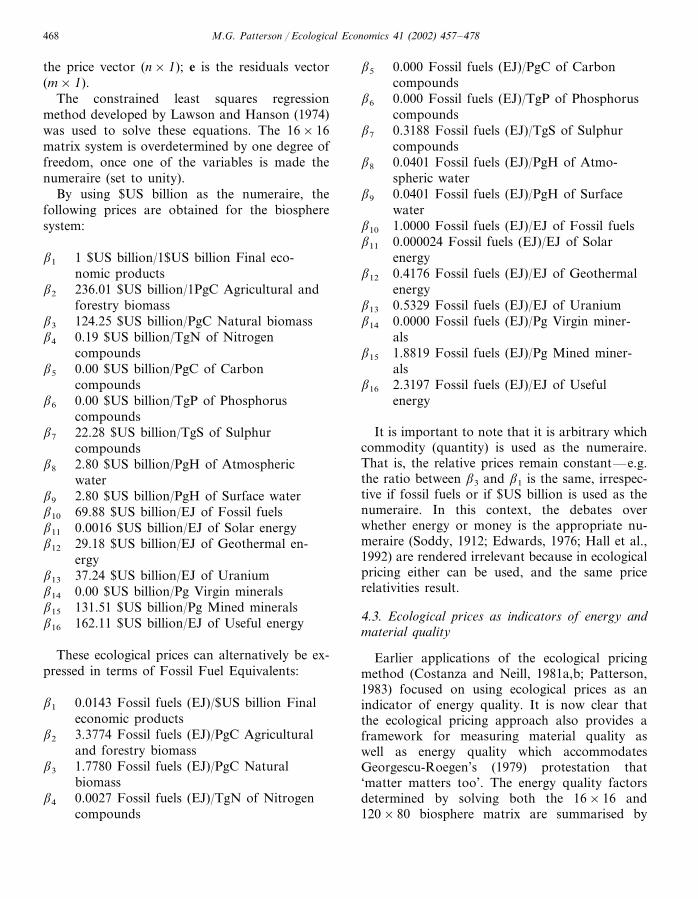
The constrained least squares regressionmethod developed by Lawson and Hanson (1974)was used to solve these equations. The 16×16matrix system is overdetermined by one degree offreedom, once one of the variables is made thenumeraire (set to unity).

By using $US billion as the numeraire, thefollowing prices are obtained for the biospheresystem:

1 $US billion/1$US billion Final eco-�1

nomic products�2 236.01 $US billion/1PgC Agricultural and

forestry biomass�3 124.25 $US billion/PgC Natural biomass

0.19 $US billion/TgN of Nitrogen�4

compounds0.00 $US billion/PgC of Carbon�5

compounds�6 0.00 $US billion/TgP of Phosphorus

compounds22.28 $US billion/TgS of Sulphur�7

compounds2.80 $US billion/PgH of Atmospheric�8

water2.80 $US billion/PgH of Surface water�9

69.88 $US billion/EJ of Fossil fuels�10

�11 0.0016 $US billion/EJ of Solar energy�12 29.18 $US billion/EJ of Geothermal en-

ergy�13 37.24 $US billion/EJ of Uranium�14 0.00 $US billion/Pg Virgin minerals

131.51 $US billion/Pg Mined minerals�15

�16 162.11 $US billion/EJ of Useful energy

These ecological prices can alternatively be ex-pressed in terms of Fossil Fuel Equivalents:

�1 0.0143 Fossil fuels (EJ)/$US billion Finaleconomic products3.3774 Fossil fuels (EJ)/PgC Agricultural�2

and forestry biomass�3 1.7780 Fossil fuels (EJ)/PgC Natural

biomass0.0027 Fossil fuels (EJ)/TgN of Nitrogen�4

compounds

0.000 Fossil fuels (EJ)/PgC of Carbon�5

compounds�6 0.000 Fossil fuels (EJ)/TgP of Phosphorus

compounds0.3188 Fossil fuels (EJ)/TgS of Sulphur�7

compounds0.0401 Fossil fuels (EJ)/PgH of Atmo-�8

spheric water�9 0.0401 Fossil fuels (EJ)/PgH of Surface

water�10 1.0000 Fossil fuels (EJ)/EJ of Fossil fuels

0.000024 Fossil fuels (EJ)/EJ of Solar�11

energy0.4176 Fossil fuels (EJ)/EJ of Geothermal�12

energy�13 0.5329 Fossil fuels (EJ)/EJ of Uranium

0.0000 Fossil fuels (EJ)/Pg Virgin miner-�14

als1.8819 Fossil fuels (EJ)/Pg Mined miner-�15

als2.3197 Fossil fuels (EJ)/EJ of Useful�16

energy

It is important to note that it is arbitrary whichcommodity (quantity) is used as the numeraire.That is, the relative prices remain constant—e.g.the ratio between �3 and �1 is the same, irrespec-tive if fossil fuels or if $US billion is used as thenumeraire. In this context, the debates overwhether energy or money is the appropriate nu-meraire (Soddy, 1912; Edwards, 1976; Hall et al.,1992) are rendered irrelevant because in ecologicalpricing either can be used, and the same pricerelativities result.

4.3. Ecological prices as indicators of energy andmaterial quality

Earlier applications of the ecological pricingmethod (Costanza and Neill, 1981a,b; Patterson,1983) focused on using ecological prices as anindicator of energy quality. It is now clear thatthe ecological pricing approach also provides aframework for measuring material quality aswell as energy quality which accommodatesGeorgescu-Roegen’s (1979) protestation that‘matter matters too’. The energy quality factorsdetermined by solving both the 16×16 and120×80 biosphere matrix are summarised by

M.G. Patterson / Ecological Economics 41 (2002) 457–478 469

Table 2Energy quality factors as measured by ecological pricesa

Ecological pricesEnergy forms

Fossil fuel $US Billion perexajoule of energyequivalents (EJ) per

exajoule of energy

Deri�ed from 16×16 matrix2.32Useful energy 162.11

69.881.00Fossil fuel29.18Geothermal 0.420.00160.00002Solarb

Deri�ed from 120×80 matrix122.70Electricity 1.76

1.10Petroleum 76.93products

Crude oil 1.03 71.7874.661.07Gas54.63Coal 0.7825.110.36Wood29.18Geothermal 0.420.00180.0002Solarb

1.64Useful heat 114.23end-usec

Transport 6.92 483.39end-usec

Obligatory 2.41 168.08electricityend-usec

Reduced fe 0.96 67.22oresc

Reduced non 2.03 141.80fe oresc

a These energy quality factors are based on the idea of‘embodied energy’. These factors should not be confused withenergy quality factors based on the ‘work potential’ of theenergy source–e.g. in exergy analysis, exergy/enthalpy is usedas an energy quality indicator. Refer to Patterson (1993) for afull discussion of energy quality indicators.

b The solar energy ecological prices do not exactly corre-spond to aggregation error.

c This is the ‘end-use’ energy portion. It is the useful energyactually produced by the end-use device, once losses have beendeducted—e.g. only about 15% of the electricity used by alight bulb is converted to useful end-use in the form ofphotons, with the remainder being converted to waste heat.

Table 3Material quality factors as measured by ecological prices

Material forms Ecological prices

Fossil fuel equivalents $US per tonne(GJ) per tonne of of materialmaterial

532 903.82Uranium 37 239 930.22146.61 10 245.42Sulphur

compoundsFossil fuels 39.68 2 773.01

8.82Final economic 616.02product

Mined minerals 131.511.88Agricultural and 1.33 92.88

forest biomassNitrogen 1.26 88.11

compoundsNatural biomass 50.110.72Atmospheric 0.002 0.16

waterSurface water 0.160.002

methods for calculating them.5 Electricity is thehighest quality energy form because more energyis required to produce electricity (backward link-ages) and because electricity is more efficient inbeing converted to useful end-use energy (forwardlinkages). Whereas solar energy is the lowest qual-ity form of energy, as it is less efficiently con-verted (than other energy sources) to usefulend-use energy.6

Energy quality in the context of ecological pric-ing is measured in terms of a ratio of value(numerator) per total heat content of the energyform (denominator). Material quality is

5 It should be noted that Odum (1983, 1996) calculated hisenergy quality factors (transformities) on the basis of back-ward linkages, whereas the ecological pricing method used inthis paper measures both backward and forward linkages.There are, however, some exceptions in Odum’s (1996)method, where he is ‘forced’ to use forward linkages forprimary inputs such as tidal energy and deep heat energy. Thisis because these primary energy inputs cannot be traced backto solar energy inputs.

6 It should be noted that previously analysts have used‘embodied energy’ (backward linkages only) as a measure ofenergy quality (e.g. Odum, 1983). The ecological pricingmethod uses both forward and backward linkages to calculateenergy quality factors.

Tables 2 and 3. These energy quality factors aresimilar to those obtained by Odum (1983, 1996)even though he uses different (non-algebraic)

M.G. Patterson / Ecological Economics 41 (2002) 457–478470

Table 4Comparison ecological prices (from the biosphere model) with market prices, 1994

Ecological priceCommodity Market price ($US per tonne) Data sources and calculation details($US per tonne)

36 376 273 Australian, Canadian and Nigerian prices37 239 930Uraniumfor 1995, (United Nations, 2000)

131Mined minerals 170 Market prices of minerals and fertilizersand fertilizers (United Nations, 2000) Quantities for the

calculation of the weighted mean price(United Nations, 1996; World ResourcesInstitute, 1996)

Surface water 0.21 (Agriculture) 0.79 (Domestic) 1.230.16 Market prices (OECD, 1998; Dinar, 2000)Quantities for the calculation of the(Industry) 0.46 (Weighted mean)weighted mean price (Postel et al., 1996)

397 ($US 10/GJ)Fossil fuel energy Market prices (International Energy2773 ($US 70/GJ)Agency, 1994)

93 (Dry weight)Agricultural and 313 (Rice) 121 (Lumber) Rice, average of Thai (two types) andforest biomass Vietnamese export prices for 1994

(United Nations, 2000) Lumber, USfutures market 1994 price (UnitedNations, 2000)

analogous, being the value (numerator) per totalmass (denominator). On this basis, there is a vastdifference in the material quality factors rangingfrom Uranium ($US 37 239 930 per tonne), toSulphur Compounds ($US 10 245 per tonne), Fos-sil Fuels ($US 2 773 per tonne), Final EconomicProduct ($US 616 per tonne), Mined Minerals($US 131.5 per tonne), Agricultural and ForestBiomass ($US 93 per tonne), Nitrogen com-pounds ($US 88 per tonne), Natural Biomass($US 50 per tonne) and finally to atmosphericsurface water ($ 0.16 per tonne). The high mate-rial quality of uranium is due to its forwardlinkage into the energy sector, which is highlyproductive in terms of producing useful energyfrom a relatively small input of mass. On theother hand, the material quality factor of FinalEconomic Product is almost entirely determinedby backward linkages in the economy, with only asmall amount of Final Economic Product beingfed back to the Agricultural and Forestry Sector.

4.4. Ecological prices and market prices

The ecological prices (derived from the bio-sphere model) can be compared with actual mar-ket prices only for those commodities that have a

market. One might expect the ecological pricesand market prices, not necessarily to be the sameor similar, but at least to be of the ‘same order ofmagnitude’ if the biosphere-pricing model is to bevalid and reliable. In fact, the mainstream inter-pretation would probably be that the ecologicalprices are ‘shadow prices’, being defined by howwell the various commodities (inputs and outputs)contribute to Value Added (column 16) in thebiosphere matrix. Another interpretation is, if themodel has good explanatory power, then the eco-logical prices and market prices should corre-spond. This approach is somewhat reminiscent ofRicardo’s attempt to ‘prove’ that labour costsexplain variations in market prices. Caution, how-ever, needs to be displayed in making either ofthese interpretations, as ecological prices aresolely determined by biophysical interdependen-cies, which although being important in definingmarket prices, they are by no means the onlyfactors.

The ecological and market prices (for the fivecommodities for which there are markets) arecompared in Table 4. There is a good correspon-dence between the two sets of prices, and certainlythe ‘ecological prices’ determined by the modelare in the ‘right’ order of magnitude. The uranium

M.G. Patterson / Ecological Economics 41 (2002) 457–478 471

prices are remarkably almost identical (ecologicalprice of $US 37.2 billion/tonne c.f. a market priceof $US 36.4 billion/tonne). The ecological pricesfor Mined Minerals and Fertilizers, Surface Waterand Agriculture and Forestry Biomass are belowthe market prices. This may be because it is verydifficult to obtain a market price for these ‘rawmaterials’ which does not include at least somecomponent of Value Added resulting from furtherprocessing or added services—hence the marketprices for these commodities in Tables 4 and 5may be slightly inflated. The most significant devi-ation between the ecological prices and marketprices is for fossil fuels where the ecological priceis seven times higher than the market price. Thisis suggesting that the market price does not reflectthe ‘true’ value of fossil fuels in terms of how wellfossil fuels contribute to economic production(Value Added) in the biosphere model. This find-ing, although apparently surprising, is consistentwith the findings of at least three other economet-ric studies. Kummel and Lindenberger (1998,2000) determined elasticities of production of

0.50, 0.45 and 0.54 for Germany, Japan and USA,respectively, implying that energy inputs at-tributed for between 45 and 54% of the economicproduction, but only had a total factor cost ($) ofabout 5%. This essentially confirms the findings ofan earlier study of the United States economy byBerndt and Wood (1987). Similarly, Patterson(1989) found that over the 1960–1984 periodenergy inputs accounted for 21.83% of GDPgrowth in New Zealand, but the energy cost shareof GDP was only 6–7%. However, it still remainslargely unexplained as to why uranium energy’secological and market prices are very similar,whereas for fossil fuels there is a sevenfolddifference.

4.5. Ecological efficiencies of biosphere processes

Having determined the ecological prices �, theecological efficiency vector � can be calculated.This involves multiplying all input and outputquantities by their appropriate prices �, to obtainthe total value of the inputs � and the total valueof the outputs �:

W�=� (4)

V�=� (5)

The elements in the gross outputs vector � arethen divided by the corresponding elements in thegross inputs vector �, to obtain the ecologicalefficiency of each process which is represented byvector �.

In ‘equilibrium’ models, all processes by defini-tion have the same efficiency, which is not thecase here in the biosphere model as the equationsare inconsistent which implies different efficienciesand ‘non-equilibrium’ ecological prices.7

In terms of ecological efficiencies, the mostinstructive information that can be extracted fromsolving the 16×16 matrix concerns the energyconversion processes:

Table 5Ecological efficiencies of biosphere processes, 1994

Processes Ecological efficiencies�

Terrestrial primary production 1.000.43Terrestrial consumption

Soil and other terrestrial processes 1.001.00Surface ocean1.00Deep ocean

Fossil fuels formation 0.33Atmosphere 1.00Natural gas use 1.40Crude oil use 0.94Hydroelectricity use 1.89Geothermal energy use 1.00Coal and wood use 0.90

1.00Uranium useMinerals and fertilizer sector 1.00

1.00Agricultural and forestry sectorOther economic sectors 1.00

Ecological efficiency � is the: total value of process outputs(price×quantity) di�ided by the total value of process inputs(price×quantity). Any quantity (solar energy, $ trillion) canbe used as the numeraire in the prices, and the same ecologicalefficiency results.

7 The assumption in such models (von Neumann, Sraffa) isthat over time ‘inefficient’ processes will be ‘out competed’,ultimately leaving an ensemble of processes, all of which havethe same profit rate (efficiency) and hence have converged atan equillibrium point.

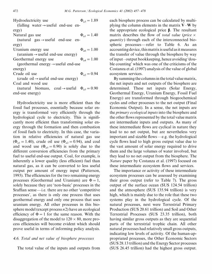
M.G. Patterson / Ecological Economics 41 (2002) 457–478472

Hydroelectricity use �a3=1.89(falling water�useful end-use en-

ergy)�a1=1.40Natural gas use

(natural gas�useful end-use en-ergy)Uranium energy use �a6=1.00

(uranium�useful end-use energy)Geothermal energy use �a4=1.00

(geothermal energy�useful end-useenergy)

�a2=0.94Crude oil use(crude oil�useful end-use energy)

Coal and wood use(natural biomass, coal�useful �a5=0.90

end-use energy)

Hydroelectricity use is more efficient than thefossil fuel processes, essentially because solar en-ergy is transformed very efficiently through thehydrological cycle to electricity. This is signifi-cantly more efficient than transforming solar en-ergy through the formation and then combustionof fossil fuels to electricity. In this case, the varia-tion in relative efficiencies of natural gas use(�a1=1.40), crude oil use (�a2=0.94), and coaland wood use (�a5=0.90) is solely due to thedifferent conversion efficiencies from the primaryfuel to useful end-use output. Coal, for example, isinherently a lower quality (less efficient) fuel thannatural gas, as it can be converted to less usefuloutput per amount of energy input (Patterson,1993). The efficiencies for the two remaining energyprocesses (Geothermal and Uranium) are �=1,solely because they are ‘non-basic’ processes in theSraffian sense— i.e. there are no other ‘competitiveprocesses’, as there is only one process that usesgeothermal energy and only one process that usesuranium energy. All other processes in this bio-sphere model (except process n2) have an ecologicalefficiency of �=1 for the same reason. With thedisaggregation of the model to 120×80, more pro-cess efficiencies will become evident which shouldprove useful in terms of informing policy analysis.

4.6. Total and net �alue of biosphere processes

The total value of the inputs and outputs from

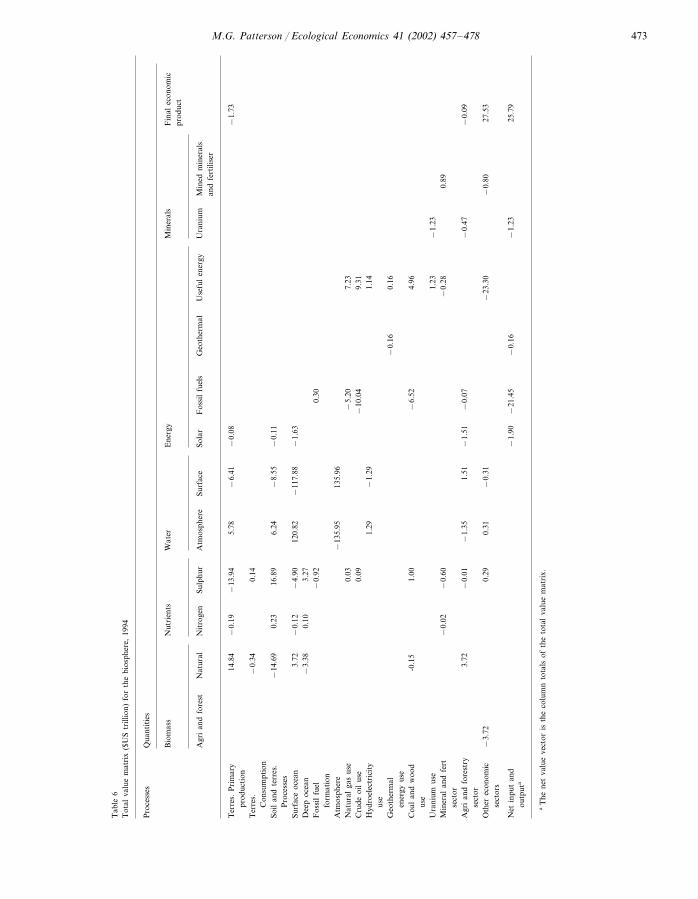
each biosphere process can be calculated by multi-plying the column elements in the matrix V–W bythe appropriate ecological price �. The resultantmatrix describes the flow of total �alue (price×quantity) through each of the interconnected bio-spheric processes—refer to Table 6. As anaccounting device, this matrix is useful as it measuresthe transfer of value through the biosphere by wayof input–output bookkeeping, hence avoiding ‘dou-ble counting’ which was one of the criticisms of theCostanza et al. (1997) analysis of the value of globalecosystem services.

By summing the columns in the total value matrix,the net inputs and net outputs of the biosphere aredetermined. These net inputs (Solar Energy,Geothermal Energy, Uranium Energy, Fossil FuelEnergy) are transformed through biogeochemicalcycles and other processes to the net output (FinalEconomic Output). In a sense, the net inputs arethe primary ecological inputs into the biosphere andthe other flows represented by the total value matrixare intermediate inputs and outputs. As many ofthese intermediate flows are cyclical in nature theylead to no net output, but are nevertheless veryimportant and sizable flows—e.g. the hydrologicalcycle flows lead to high gross output value due tothe vast amount of solar energy required to drivethem and the large volumes of water involved, butthey lead to no net output from the biosphere. TheNature paper by Costanza et al. (1997) focused onthese intermediate ecosystem flows and services.

The importance or activity of these intermediateecosystem processes can be assessed by examiningtheir gross output (refer to Table 7). The grossoutput of the surface ocean ($US 124.54 trillion)and the atmosphere ($US 135.94 trillion) is veryhigh, which is mainly due to the role that these twosystems play in the hydrological cycle. Of thenatural processes, next were Terrestrial PrimaryProduction ($US 20.61 trillion) and Soil and OtherTerrestrial Processes ($US 23.35 trillion), bothhaving similar gross outputs as they are sequentialparts of the terrestrial trophic chain. All othernatural processes had relatively small gross outputs,indicating low levels of activity. Of the human-ap-propriated processes, the Other Economic Sectors($US 28.13 trillion) and the Energy Sector processes($US 26.45 trillion) had the highest gross output.

M.G. Patterson / Ecological Economics 41 (2002) 457–478 473

Tab

le6

Tot

alva

lue

mat

rix

($U

Str

illio

n)fo

rth

ebi

osph

ere,

1994

Pro

cess

esQ

uant

itie

s

Ene

rgy

Min

eral

sF

inal

econ

omic

Nut

rien

tsW

ater

Bio

mas

spr

oduc

t

Surf

ace

Sola

rF

ossi

lfu

els

Geo

ther

mal

Use

ful

ener

gyU

rani

umN

itro

gen

Min

edm

iner

als

Sulp

hur

Atm

osph

ere

Nat

ural

Agr

ian

dfo

rest

and

fert

ilise

r

−0.

19−

13.9

45.

78−

6.41

−0.

08−

1.73

Ter

res.

Pri

mar

y14

.84

prod

ucti

onT

erre

s.−

0.34

0.14

Con

sum

ptio

n16

.89

6.24

−8.

55−

0.11

−14

.69

Soil

and

terr

es.

0.23

Pro

cess

es−

117.

88−

1.63

120.

82−

0.12

−4.

90Su

rfac

eoc

ean

3.72

−3.

380.

103.

27D

eep

ocea

n−

0.92

0.30

Fos

sil

fuel

form

atio

n13

5.96

−13

5.95

Atm

osph

ere

−5.

207.

23N

atur

alga

sus

e0.

03−

10.0

49.

31C

rude

oil

use

0.09

1.29

−1.

291.

14H

ydro

elec

tric

ity

use

−0.

160.

16G

eoth

erm

alen

ergy

use

−6.

524.

96C

oal

and

woo

d1.

00-0

.15

use

1.23

−1.

23U

rani

umus

e−

0.02

−0.

60−

0.28

0.89

Min

eral

and

fert

sect

or−

1.35

1.51

−1.

51−

0.07

−0.

473.

72−

0.09

−0.

01A

gri

and

fore

stry

sect

or0.

31−

0.31

−23

.30

−0.

80O

ther

econ

omic

27.5

3−

3.72

0.29

sect

ors

−1.

90−

21.4

5−

0.16

−1.

2325

.79

Net

inpu

tan

dou

tput

a

aT

hene

tva

lue

vect

oris

the

colu

mn

tota

lsof

the

tota

lva

lue

mat

rix.

M.G. Patterson / Ecological Economics 41 (2002) 457–478474

Table 7Total output of biosphere processes, 1994 ($US trillion)

Process Total output ($UStrillion)

20.61Terrestrial primary productionTerrestrial consumption 0.15Soil & other terrestrial 23.35

processes124.54Surface ocean

3.37Deep ocean0.31Fossil fuel formation

Atmosphere 135.967.26Natural gas use

Crude oil use 9.41Hydroelectricity use 2.43

0.16Geothermal energy useCoal and wood use 5.97Uranium use 1.23Minerals and fertilizer sector 0.89Agricultural and forestry sector 5.23

28.13Other economic sectors

methods often used in valuation and cost-benefitstudies (Cleveland et al., 1984; Costanza et al.,1991; Proops, 2000). Ecological pricing as devel-oped in this paper is seen as a constructive movein this direction, being based on measuring biophys-ical interdependencies (or contributory values) im-plicit in the global ecological system and itseconomic sub-system. Although some of thesebiophysical interdependencies are clearly a result ofhuman interventions and hence indirectly reflecthuman preferences, ecological pricing does how-ever tend to highlight species and ecological func-tions that may not usually be detected by othervaluation methods such as WTP (Costanza, 1991).For example, it is unlikely that the value ofprotozoa in the ecosystem would be measured in aWTP survey, whereas in ecological pricing thevalue of these protozoa would be taken account ofby the forward and backward linkages they havewith other components of the ecosystem. In thissense, ecological pricing is more ‘biocentric’ thanneoclassical valuation methods that tend to have amore anthropocentric emphasis (Hannon, 1998).

In the spirit of methodological pluralism, ecolog-ical pricing is not seen as a replacement for neoclas-sical valuation, or for that matter, other valuationmethods. Rather, it is seen as a complementaryapproach not to be used instead of the othermethods, but alongside other methods. Or indeedecological pricing could be used as a component ofa multicriteria framework or methodologicalschema such as that proposed by Lockwood (1997).

Although the ecological pricing method devel-oped in this paper has a number of antecedents andcommonalities with methods used both in econom-ics and ecology, it is unique in a number of ways.Firstly, it is based on a non-equilibrium model ofpricing, insofar that there is no a priori assumptionthat the system is (or should be) at equilibrium asdo the pricing models of von Neumann (1945),Sraffa (1960), Leontief (1986), and Costanza andHannon (1989). That is, particularly in very disag-gregrated models where there are more processesthan quantities, it is almost inevitable that we willbe dealing with inconsistent equations, whichmeans that processes will have differing efficiencies.Equilibrium conditions are just an artifact of solv-ing a square matrix (m=n) of equations—or of

The Costanza et al. (1997) analysis concludedthat global ecosystem services had a total value of1.32 times the value of goods and services producedby the global economy.8 Several commentatorsargued that this ratio of ‘value of ecosystem ser-vices:GDP’ was too high, as on theoretical groundsit should not exceed one (Ayres, 1998; Pearce,1998). Interestingly, the biosphere pricing modelpresented in this paper, shows that the value ofprimary ecological inputs is $24.73 trillion, com-pared with $25.79 trillion for global GDP, givinga ratio of 0.98.

5. Discussion

A recurrent theme in the ecological economicsliterature is the call for valuation and pricingmethods that are more biophysical/biocentric toprovide a counterbalance to the anthropocentric

8 The original Costanza et al. (1997) analysis estimated thevalue of global ecosystem services to be $33 trillion for 1994(c.f. $18 trillion for global GDP), giving a ratio of 1.83.Subsequently, it has been estimated that the value of globalGDP for 1994 was about $25 trillion (World Bank, 1996),giving a ratio of 1.32 which is used above.

M.G. Patterson / Ecological Economics 41 (2002) 457–478 475

solving a matrix that has been reduced to a‘square’ form by using an optimization method.Secondly, it is clear that it is not necessary thatsolar energy be used as the numeraire, as assumedin previous pricing models used in ecology. Anyquantity (commodity) can be used as the nu-meraire and the relative prices remain constant, asdo other system parameters, such as the ecologicalefficiencies of processes. Indeed, the EconomicOutput quantity ($ value added) can be used asthe numeraire if so desired— this may be impera-tive in terms of ‘communicating’ the results of anyecological pricing exercise. Thirdly, and related tothe last point, the ecological prices can be ex-pressed in terms of monetary units, solar energyunits (Emergy), or land equivalents (EcologicalFootprint). All of these numeraires essentiallygive the same analytical result, but they communi-cate to different disciplinary audiences. Express-ing the results of any ecological pricing exercise interms of these alternative numeraires, may well bea fruitful tactic in terms of encouraging communi-cation across these disciplinary boundaries.

The main empirical finding of this paper is thatthe ratio of the ‘value of primary ecological inputsto Global GDP’ was found to be 0.98 for 1994.This compares with a ratio of 1.32 for the ‘valueof global ecosystems: global GDP’ determined byCostanza et al. (1997) in their Nature paper forthe same year. One reason, why our study arrivedat a lower ratio, may be that the input–outputaccounting eliminates double counting, by tracingthe flow of value through the system to arrive ata net figure. In the Costanza et al. (1997) study itis possible that some of the ecosystem servicesmay be overlapping, or one ecosystem service maycontribute to another ecosystem service and hencebe ‘double-counted’. Another important empiricalfinding was that the ecological prices (with theexception of fossil fuels) show a good correspon-dence with actual market prices for those prod-ucts that are traded on markets. The exception offossil fuels is not surprising, even though theecological price is about seven times the marketprice. This is because econometric studies havefound that energy inputs contribute in the orderof five-seven times more to GDP growth thantheir cost share indicates.

Acknowledgements

This work was conducted as part of the Work-ing Group on the Value of the World’s EcosystemServices and Natural Capital; Toward a Dynamic,Integrated Approach supported by the NationalCenter for Ecological Analysis and Synthesis, aCenter funded by NSF (Grant cDEB-0072909),the University of California, and the Santa Bar-bara campus. Additional support was also pro-vided for the Postdoctoral Associate, Matthew A.Wilson, in the Group. The discussions held withfellow ‘Theory Group’ members (Steve Farber,Matt Wilson, Karin Limburg, Bob O’Neill,Rudolph de Groot, Richard Howarth, Glen-Marie Lange) during our NCEAS Santa Barbarameetings in 1998 and 1999 proved particularlyvaluable as input into this paper. A special thanksis also due to Bob Costanza for his useful com-ments and suggestions concerning an initial draftof this paper. I am also grateful to two anony-mous referees who provided detailed and helpfulnotes on the submitted draft of this paper.

The financial support from the New ZealandFoundation of Research Science and Technology(Contract C09X0007) is also acknowledged andmuch appreciated.

References

Amir, S., 1989. On the use of ecological prices and systems-wide indicators derived there from to quantify man’s im-pact on the ecosystem. Ecological Economics 1, 203–231.

Amir, S., 1994. The role of thermodynamics in the study ofeconomic and ecological systems. Ecological Economics10, 125–142.

Ayres, R.U., 1996. Industrial Metabolism and the GrandNutrient Cycles. INSEAD, Fontainebleau, France.

Ayres, R.U., 1998. The price–value paradox. Ecological Eco-nomics 25, 17–19.

Berndt, E.R., Wood, D.O., 1987. Energy price shocks andproductivity growth: a survey. In: Gordon, R.L., Jacoby,H.D., Zimmerman, M.B. (Eds.), Energy: Markets andRegulation. MIT Press, Cambridge, MA, pp. 305–387.

Bowen, H.J.M., 1979. Environmental Chemistry of the Ele-ments. Academic Press, London.

British Petroleum, 1996. BP Statistical Review of World En-ergy 1996. British Petroleum, London.

Butcher, S., Charlson, K.J., Orians, G.H., Wolfe, G.V., 1992.Global Biogeochemical Cycles. Academic Press, London.

M.G. Patterson / Ecological Economics 41 (2002) 457–478476

Cleveland, C.J., Costanza, R., Hall, C.A.S., Kaufmann, R.,1984. Energy in the United States economy: a biophysicalperspective. Science 225, 890–897.

Collins, D., Odum, H.T., 2001. Calculating transformitieswith an Eigenvector method. In: Brown, M.T. (Ed.),Emergy Synthesis: Theory and Applications of theEmergy Methodology. Center for Environmental Policy,University of Florida, Gainesville, pp. 265–279.

Costanza, R., 1991. Energy, uncertainty and ecological eco-nomics. In: Physical Chemistry. Proceedings of an Inter-national Workshop, Siena, Italy. Elsevier, Amsterdam,pp. 203–207.

Costanza, R., Neill, C., 1981a. The energy embodied in prod-ucts of the biosphere. In: Mitsch, W.J., Boserman, R.W.,Klopatek, J.M. (Eds.), Energy and Ecological Modelling.Elsevier, Amsterdam, pp. 745–755.

Costanza, R., Neill, C., 1981b. Energy embodied in productsof ecological systems: a linear programming approach. In:Mitsch, W.J., Boserman, R.W., Klopatek, J.M. (Eds.),Energy and Ecological Modeling. Elsevier, Amsterdam.

Costanza, R., Neill, C., 1984. Energy intensities, interdepen-dence and value in ecological systems: a linear program-ming approach. Journal of Theoretical Biology 106,41–57.

Costanza, R., Hannon, B., 1989. Dealing with the mixedunits problem in ecosystem network analysis. In: Wulff,F., Field, J.G., Mann, K.H. (Eds.), Network Analysis inMarine Ecology: Methods and Applications. Springer,Berlin, pp. 90–115.

Costanza, R., Neill, C., Leibowitz, S.G., Fruci, J., Bhar, L.,Day, J.W., 1983. Ecological Models of the MississippiDelta Plain Region: Data Collection and Presentation.Fish and Wild Life Services, US Department of Interior,Washington.

Costanza, R., Daly, H.E., Bartholomew, J.A., 1991. Goals,agenda and policy recommendations for ecological eco-nomics. In: Costanza, R. (Ed.), Ecological Economics:The Science and Management of Sustainability. ColumbiaUniversity Press, New York, pp. 1–20.

Costanza, R., d’Arge, R., de Groot, R., Farber, S., Grasso,M., Hannon, B., Limburg, K., Naeem, S., O’Neill, R.V.,Paruelo, J., Raskin, R.G., Sutton, P., van der Belt, M.,1997. The value of the world’s ecosystem services andnatural capital. Nature 387 (15), 253–260.

Daly, H.E., 1985. The circular flow of exchange value andlinear throughput of matter-energy: a case of misplacedconcreteness. Review of Society and Economy XLII (3),279–297.

DeAngelis, D.L., Waterhouse, J.C., 1987. Equilibrium andnon equilibrium concepts in ecological models. EcologicalMonographs 57, 1–21.

den Elzen, M., Beusen, A., Rotmans, J., 1995. ModellingGlobal Biogeochemical Cycles: An Integrated Approach.National Institute of Public Health and the Environment(RIVM). Bilthoven, The Netherlands.

Dinar, A., 2000. The Political Economy of Water PricingReforms. Oxford University Press, Oxford.

Edwards, G.W., 1976. Energy budgeting: joules or dollars.Australian Journal of Agricultural Economics 20, 179–191.

Energy Efficiency and Conservation Authority, 1997. EnergyEnd-Use Database. EECA, Wellington, New Zealand.

England, R.W., 1986. Production, distribution and environ-mental quality: Mr Sraffa reinterpreted as an ecologist.Kyklos 39, 230–244.

Farber, S., Costanza, R., Wilson, M., 2002. Economic andEcological Concepts for Valuing Ecosystem Services.

Fruci, J.R., Costanza, R., Leibowitz, S.G., 1983. Quantifyingthe interdependence between material and energy flows inecosystems. In: Laurenroth, W.K., Skogerboe, G.V., Flug,M. (Eds.), Analysis of Ecological Systems: State-of-the-Art in Ecological Modelling. Elsevier, Amsterdam, pp.241–250.

Gale, D., 1960. The Theory of Linear Economic Models.McGraw Hill, New York.

Georgescu-Roegen, N., 1979). Energy analysis and economicvaluation. Southern Economy Journal 45, 1023–1058.

Gilliland, M.W., 1975. Energy analysis and public policy.Science 189, 1051–1056.

Gilliland, M., 1977. Energy analysis: a tool for evaluating theimpact of end-use management strategies on economicgrowth. In: Fazzolare, R.A., Smith, C.B. (Eds.), EnergyUse Management. Proceedings of the International Con-ference. Pergamon Press, New York, pp. 613–619.

Hall, C.A.S., Cleveland, C.J., Kaufmann, R., 1992. Energyand Resource Quality: The Ecology of the Economic Pro-cess. University Press of Colarado, Colarado.

Hannon, B., 1998. How might nature value man. EcologicalEconomics 25, 265–279.

Heuttner, D.A., 1976. Net energy analysis: an economic as-sessment. Science 192, 101–104.

Hubbert, M.K., 1963. Energy resources. A Report to theCommittee on Natural Resources of the NaturalAcademy of Sciences-National Research Council, Wash-ington, DC.

International Energy Agency, 1987. Electricity End-Use Effi-ciency. IEA, Paris.

International Energy Agency, 1994. Energy Prices and Taxes:2nd Quarter 1994. IEA, Paris.

International Energy Agency, 1997. Energy Statistics andBalances of Non-OECD Countries 1994–1995. IEA,Paris.

Jorgensen, S.E., 1998. Exergy as an orientor of the develop-ment of ecosystems. In: Advances in Energy Studies: En-ergy Flows in Ecology and Economy. Museum of Scienceand Scientific Information, Rome, pp. 371–402.

Judge, G.C., Takayama, T., 1966. Inequality restrictions inregression analysis. Journal of the Statistical Association61, 166–181.

Judson, D.H., 1989. The convergence of neo-ricardian andembodied energy theories of value and price. EcologicalEconomics 1, 261–281.

Koopmans, T., 1951. Activity Analysis of Production andAllocation. Wiley, New York.

M.G. Patterson / Ecological Economics 41 (2002) 457–478 477

Kummel, R., Lindenberger, D., 1998. Energy, technical pro-gress and industrial growth. In: Advances in EnergyStudies: Energy Flows in Ecology and Economy. Mu-seum of Science and Scientific Information, Rome, pp.207–222.

Kummel, R., Lindenberger, D., 2000. Productive power ofenergy and economic evolution. Indian Journal of Ap-plied Economics 8, 231–262.

Lawson, C.L., Hanson, R.J., 1974. Solving Least SquaresProblems. Society for Industrial and Applied Mathemat-ics. Prentice Hall, New Jersey.

Leontief, W., 1986. Input–output Economics. Oxford Uni-versity Press, New York.

Lockwood, M., 1997. Integrated value theory for naturalareas. Ecological Economics 20, 83–93.

Lotka, A.J., 1922). Natural selection as a physical principle.Proceedings of the National Academy of Science 8, 147–151.

Lotka, A.J., 1925). Physical Biology. Williams and Wilkins,Baltimore.

Malinvaud, E., 1953. Capital accumulation and efficient allo-cation of resources. Econometrica 21, 233–269.

O’Connor, M., 1996. Cherish the future, cherish the other:A post classical theory of value. In: Faucheaux, S.,Pearce, D., Proops, J. (Eds.), Models of Sustainable De-velopment. Edward Elgar, Cheltenham, pp. 321–345.

Odum, H.T., 1971. Environment, Power and Society. Wiley,New York.

Odum, H.T., 1983. Systems Ecology: An Introduction. Wi-ley, New York.

Odum, H.T., 1996. Environmental Accounting: EMERGYand Environmental Decision Making. Wiley, New York.

Odum, H.T., 2000. Handbook of Emergy Evaluation: En-ergy of Global Processes-Folio c2. Center for Environ-mental Policy, University of Florida, Gainesville.

Odum, H.T., Odum, E.C., 1976. Energy Basis for Man andNature. McGraw-Hill, New York.

Odum, H.T., Brown, M.T., Brandt-Williams, S., 2000.Handbook of Emergy Evaluation: Introduction andGlobal Budget-Folio cI. Center for Environmental Pol-icy, University of Florida, Gainesville.

Oort, A.H., 1970. The energy cycle of the earth. ScientificAmerican 223, 54–63.

Organisation of Economic Co-operation and Develop-ment,1998. Pricing of Water-Services in OECD Coun-tries: Synthesis Report. Document 69368. Group onEconomic and Environment Policy Integration, Environ-ment Directorate, Paris.

Patterson, M.G., 1983. Estimation of the quality of energysources and uses. Energy Policy 11, 346–359.

Patterson, M.G., 1989. Energy, Productivity and EconomicGrowth: An Analysis of New Zealand and OverseasTrends. Market Analysis Report 89/1006. Ministry ofEnergy, Wellington.

Patterson, M.G., 1991. A Systems Approach to EnergyQuality and Efficiency. Unpublished revision of a PhD

thesis, School of Architecture, Victoria University ofWellington, New Zealand.

Patterson, M.G., 1993. Approaches to energy quality in en-ergy analysis. International Journal of Global Energy Is-sues 5, 19–28.

Patterson, M.G., 1996. What is energy efficiency? Concepts,indicators and methodological issues. Energy Policy 24,377–390.

Patterson, M.G., 1998a. Commensuration and theories ofvalue in ecological economics. Ecological Economics 25,105–123.

Patterson, M.G., 1998b. Understanding energy quality inecological and economic systems. In: Advances in EnergyStudies: Energy Flows in Ecology and Economy. Mu-seum of Science and Scientific Information, Rome, pp.257–274.

Pearce, D., 1998. Auditing the earth: the value of theworld’s ecosystem services and natural capital. Environ-ment 40, 23–28.

Perrings, C., 1987. Economy and Environment: A Theoreti-cal Essay of the Interdependencies of Economic and En-vironmental Systems. Cambridge University Press, NewYork.

Perrings, C., 1996. Ecological resilience in the sustainabilityof economic development. In: Faucheaux, S., Pearce,D.W., Proops, J. (Eds.), Models of Sustainable Develop-ment. Edward Elgar, London, pp. 231–252.

Pimm, S.L., 1991. The Balance of Nature? Ecological Issuesin the Conservation of Species and Communities. Uni-versity of Chicago Press, Chicago.

Postel, S., Daily, G.C., Ehrlich, P., 1996. Human appropria-tion of renewable freshwater. Science 27, 785–787.

Proops, J., 2000. Research Challenges for Ecological Eco-nomics in the 21st Century. Paper Presented to the SixthBiennial Meeting of the International Society for Ecolog-ical Economics 5–8 July 2000, Canberra, Australia.

Schlesinger, W.H., 1991. Biogeochemistry: An Analysis ofGlobal Change. Academic Press, San Diego.

Shiklomanov, I.A., 1993. World water resources. In: Gleick,D.H. (Ed.), Water in Crisis: A Guide to the World’sFresh Water Resources. Oxford University Press, NewYork, pp. 13–24.

Slesser, M., 1973. Energy analysis in policy making. NewScientist, November, pp. 328–330.

Soddy, F., 1912. Matter and Energy. Williams and North-gate, London.

Sraffa, P., 1960. Production of Commodities by Means ofCommodities: Prelude to a Critique of Economic Theory.Cambridge University Press, Cambridge.

Stigler, G.J., 1965. Essays in the History of Economics. Uni-versity of Chicago Press, Chicago.

Stout, B.A., 1990. Handbook of Energy for World Agricul-ture. Elsevier Applied Science, London.

United Nations, 1993. Trends in International Distributionof Global World Product. United Nations, New York.

M.G. Patterson / Ecological Economics 41 (2002) 457–478478

United Nations, 1996. Industrial Commodities Statistics Year-book. United Nations, New York.

United Nations, 2000. World Commodity Survey 1999–2000.Markets, Trends and the World Economic Environment.United Nations, New York.

Victor, P.A., 1972). Pollution: Economy and Environment.Allen and Unwin, London.

von Neumann, J., 1945. A model of general equilibrium.Review of Economic Studies 13, 1–9.

Wake, G., McKibbin, R., Cole, A., Patterson, M.G., 1998.

Ecological pricing: an eigenvalue–eigenvector solutionmethod. Working Paper, Department of Resource andEnvironmental Planning, Massey University, PalmerstonNorth, New Zealand.

Wigley, T.M.L., Schimel, D.S., 2000. The Carbon Cycle. Cam-bridge University Press, Cambridge.

World Bank, 1996. The World Bank Atlas, World Bank,Washington, DC.

World Resources Institute, 1996. World Resources 1996–1997.Oxford University Press, New York.