ecological fiscal reform and energy case study on renewable grid...
TRANSCRIPT

Marbek Resource Consultants Ltd. 300-222 Somerset Street West, Ottawa, ON K2P 2G3
Tel: 613.523.0784 Fax: 613.523.0717 www.marbek.ca
ECOLOGICAL FISCAL REFORM AND ENERGY CASE STUDY ON RENEWABLE GRID-POWER
ELECTRICITY
–Final Baseline and Economic Report–
Submitted to:
National Round Table on Environment and Economy
Submitted by:
Marbek Resource Consultants
In association with:
May 21, 2004

Table of Contents
1. INTRODUCTION..............................................................................................................1
1.1 Objectives and Scope of this Case Study.................................................................1 1.2 Data Sources ............................................................................................................2 1.3 Presentation of this Report.......................................................................................2
2. BACKGROUND AND CONTEXT..................................................................................3
2.1 Introduction..............................................................................................................3 2.2 The Policy Context - Encouraging Carbon-Reducing Technology .........................3 2.3 The Fiscal Instrument Context - Encouraging Carbon-Reducing Technology .......4 2.4 The Renewable Energy Technologies Context........................................................6 2.5 The Modelling Context ..........................................................................................11
3. RENEWABLE GRID POWER IN CANADA ..............................................................12
3.1 Introduction............................................................................................................12 3.2 Current Grid-Power RET Status in Canada ...........................................................12 3.3 Future Potential for Grid-Power RETs in Canada .................................................17 3.4 Technology Costs and Learning Trends ................................................................19 3.5 Creation of Model’s Grid-Power RET Supply Curve............................................20
4. THE ELECTRICAL SECTOR BASELINE.................................................................22
4.1 Introduction............................................................................................................22 4.2 Geographical Coverage..........................................................................................22 4.3 Time Period............................................................................................................22 4.4 Discount Rate and Dollar Year ..............................................................................23 4.5 Marginal Cost of Fossil Fuel Generation...............................................................23 4.6 Baseline Emissions Intensity of Fossil Fuel Generation........................................23 4.7 Carbon Abatement Cost Curve for Fossil Fuel Generation ...................................25 4.8 Price Elasticity of Demand for Electricity .............................................................27 4.9 Return on R&D Investment (ROI).........................................................................27 4.10 Current Expenditures on Renewables R&D in Canada .........................................28 4.11 Baseline Demand for Electricity from Fossil Fuel ................................................29 4.12 Baseline of Annual Renewable Energy Supplied ..................................................30 4.13 Carbon Price...........................................................................................................31
5. ECONOMIC AND POLICY ANALYSIS - APPLICATION TO CANADA.............32
5.1 Introduction............................................................................................................32 5.2 Overview of Fiscal Instruments Assessed .............................................................32 5.3 Overview of RFF Renewables Uptake Model .......................................................33 5.4 Summary of Results...............................................................................................35 5.5 Discussion of the Base Case and Fiscal Instruments .............................................39 5.6 Sensitivity Analysis ...............................................................................................48 5.7 Conclusion .............................................................................................................52
Appendix A: Survey of Renewable Energy Fiscal Instruments Appendix B: Overview of the Model Appendix C: References, Assumptions, and Notes on Grid-Power RET Resources
EFR & Energy Case Study on Renewable Grid Power Electricity ─ Baseline & Economic Report ─
Marbek Resource Consultants/Resource for the Future Page 1
1. INTRODUCTION The National Round Table on the Environment and the Economy (NRTEE) has initiated a program to examine the role of Ecological Fiscal Reform (EFR) in meeting the challenges of implementing sustainable development in Canada. Results of the first phase of the EFR program, which focussed on the agricultural, transportation and chemical sectors, concluded that fiscal policy is one of the most powerful means at the government’s disposal to influence outcomes in the economy; if used in a consistent and strategic manner, EFR can promote objectives that have simultaneous economic and environmental benefits. In the spring of 2003, the NRTEE launched the second phase of its EFR program with a focus on the potential contribution of EFR to reducing carbon dioxide (CO2) emissions from energy. The goal of this second phase is to “examine how to reduce energy-based carbon emissions, both in absolute terms and as a ratio of GDP, using fiscal policy without increasing other pollutants.” Consistent with the approach employed in the previous phase, this phase of the EFR program includes the development of case studies on three sectors that can contribute significantly to “decarbonisation” of Canada’s energy sector, namely: renewable energy, hydrogen and energy efficiency. 1.1 OBJECTIVES AND SCOPE OF THIS CASE STUDY This case study provides an analysis of the role that fiscal policy can play in promoting the long-term development of Canada’s renewable energy sector, with a view of promoting and, where appropriate, accelerating the use of renewable energy technologies that leads to long-term reductions in energy-based carbon emissions. This case study addresses the renewable energy (RE) sector1 and explores the ‘traction” of fiscal instruments to improve the uptake or deployment of grid-power renewable energy technologies (RETs) in Canada. Consistent with the broader goal of the EFR program, the objectives of this case study are twofold: To deliver pragmatic, policy-relevant recommendations on how fiscal policy can be used
to promote sustainable development; and To synthesize the lessons learned from each case study into a “State of the Debate” report
that will assess the potential use of fiscal policy in promoting long-term decarbonisation. In pursuit of these objectives, the case study follows a step-wise approach that: Defines a renewable and electrical energy baseline in the years 2010, 2020 and 2030 Defines a GHG emissions baseline for electrical energy Identifies a set of renewable energy fiscal instrument scenarios Models a set of fiscal instruments; and, Assesses the relative environmental and economic implications of the fiscal instruments.
1 Separate case studies are being prepared for the other two sectors under separate contracts.

EFR & Energy Case Study on Renewable Grid Power Electricity ─ Baseline & Economic Report ─
Marbek Resource Consultants/Resource for the Future Page 2
1.2 DATA SOURCES The development of this case study involved the compilation and analysis of a large amount of data. Many of the data inputs that are required for modelling purposes in this case study are, in fact, the outputs from large and complex studies that themselves are based on numerous assumptions. Throughout this case study, data sources are clearly indicated and detailed references are provided in the attached appendices. In each case, the selection of data sources was guided by three key principles: Data should be as recent as possible Data need to be from credible and impartial sources; and To the extent possible, data used in this case study should be from a consistent set of
sources. For example, the estimation of on-margin emissions reductions used herein is based on a large study conducted for Environment Canada. That same study also estimated future electricity generation costs as part of developing the on-margin emission impacts. This case study requires both data sets (i.e., emission reductions and fossil fuel generating costs) and therefore draws both from the same study results.
Completion of this case study also required a number of data inputs (e.g., renewable resource size) where the available information is incomplete. In these cases, the approach was to draw on the best available data and to augment this data with consultations involving selected Canadian experts. 1.3 PRESENTATION OF THIS REPORT Following this introductory section, the remainder of this case study is presented as follows: Section 2 provides the context in which this study is implemented, including a discussion
of the policy, fiscal instruments, renewable energy technologies and the modelling context.
Section 3 provides a discussion of the baseline renewable power sector, including an overview of its current technological status as well as forecasts of expected resource availability and costs.
Section 4 identifies the baseline electrical sector parameters, including the price of electricity, the baseline market share of renewables and fossil fuels in overall generation, and the cost of carbon reductions. As well, a number of important baseline analytical assumptions are identified including time frame, geographic coverage, discount rates, and dollar years.
Section 5 presents the case study results of the economic modelling as well as sensitivity testing of key variables.
The synthesis of lessons learned, as noted in the objectives above, is provided in a separate report.

EFR & Energy Case Study on Renewable Grid Power Electricity ─ Baseline & Economic Report ─
Marbek Resource Consultants/Resource for the Future Page 3
2. BACKGROUND AND CONTEXT 2.1 INTRODUCTION This section provides a brief discussion of four areas that are particularly relevant to setting this case study in its proper context. They are: The policy context provides an overview of why fiscal instruments are needed to assist
with achieving societal objectives such as decarbonising the economy or improving the uptake of renewable technologies
The EFR instrument context provides an overview of the types of fiscal instruments that have been applied internationally
The renewable energy context defines the grid-power renewable energy technologies that are included in this study
The modeling context provides a brief overview of how the likely impacts of alternative fiscal instrument are assessed against a number of indicators such as cost, renewables uptake and electricity prices.
Each point is discussed in turn below. 2.2 THE POLICY CONTEXT - ENCOURAGING CARBON-REDUCING
TECHNOLOGY
With greenhouse gas emissions a growing policy concern, much attention is being given to the potential for renewable energy to displace fossil fuel sources. In 2001, out of the total primary energy supply for the OECD countries, renewable energy sources provided 5.7%, of which 54% was supplied by combustible renewables and waste,2 35% by hydro power, and 12% by geothermal, solar, wind and tide energy. For electricity generation, renewables represented 15% of production worldwide, but only 2.1% if one excludes hydro. The United States aims to nearly double energy production from renewable sources (excluding hydro) compared to 2000 levels by 2025.3 Meanwhile, the European Union has given itself the target of achieving 22.1% of electricity produced from renewable energy and 12% of renewables in gross national energy consumption, by 2010.
In Canada, the Climate Change Action Plan identifies the following renewable energy programs and targets:
An incentive for wind power production (2.8 MT) Green power purchases for 20% of the Government of Canada’s electricity needs (0.2
MT) A target of 10 % of new electricity generating capacity to be from emerging renewable
sources (3.9 MT); and Identify and develop options to address impediments to new regional hydroelectricity
transmission and generation capacity. 2 This category includes biomass and excludes trash and nonrenewable waste. 3 The Department of Energy Strategic Plan, “Protecting National, Energy, and Economic Security with Advanced Science and Technology and Ensuring Environmental Cleanup,” Draft: August 6, 2003.

EFR & Energy Case Study on Renewable Grid Power Electricity ─ Baseline & Economic Report ─
Marbek Resource Consultants/Resource for the Future Page 4
Given such ambitious targets, a great deal of focus has been placed on the role of incentives in promoting technological innovation and lowering the cost of non-emitting energy sources. To reduce greenhouse gas emissions by promoting the technological development and diffusion of renewable energy, recent policies and proposals employ a broad range of incentives. Some focus on reducing the cost of research and development (R&D) and of investment, such as a tax credit for R&D or subsidies for capital costs. Others try to ensure viable markets for the environmentally desirable technology, such as a generation subsidy for renewable energy or a portfolio (market share) requirement for renewable sources. Alternatively, some policies create disincentives for non-renewable energy sources, by taxing energy (while exempting renewable sources) or by making greenhouse gas emissions expensive, such as with a tradable emissions permit system, carbon tax, or emissions intensity standard for generation. Although economists typically argue that a direct price for carbon (via a tax or tradable permit system) would provide the most efficient incentives for development and use of less emitting technologies, the diversity of the present policy portfolio suggests that other forces are at play. First, emissions pricing policies that risk significantly reducing economic activity have little appeal to most governments. Second, the distributional consequences of raising the price of carbon can be important, particularly for energy intensive industries, owners of fossil fuel generation sources, and consumers. Third, failures in the market for innovation, such as spillover effects, imply that emissions pricing alone will not provide sufficient incentive to improve technologies. Finally, the process of technological advancement can take place not only through R&D investments, but also via learning through the production and use of technologies; thus, encouraging output may also spur innovation. Consequently, subsidies—and output support strategies in particular—are often attractive to decision-makers and play an important role alongside emissions regulations and R&D policies. In the next section, the fiscal instrument options that can improve renewables uptake are more precisely defined. 2.3 THE FISCAL INSTRUMENT CONTEXT - ENCOURAGING CARBON-
REDUCING TECHNOLOGY Using fiscal instruments to shift the economy onto a path that balances environmental, social and economic goals is certainly not a new paradigm. Long before the concept of sustainable development was adopted as a global imperative, economic and environmental management theory came to recognize that fiscal instruments could be used to send market signals to achieve environmental objectives. Since the mid-1960s, fiscal instruments have been recognized as a cost-effective alternative and/or complement to command-and-control systems to achieve environmental goals. The fundamental difference between fiscal instruments and command-and-control regulatory approaches is that compliance decisions are shifted from the regulator to the regulated community. This shifting of compliance decision-making to the targeted community (i.e., firms) in theory provides increased flexibility. It is this increased flexibility that allows decisions to be made that minimize compliance costs and thus maximize profits. According to environmental

EFR & Energy Case Study on Renewable Grid Power Electricity ─ Baseline & Economic Report ─
Marbek Resource Consultants/Resource for the Future Page 5
economic theory, enabling this profit-maximizing behaviour is a major attraction of fiscal instruments over more traditional regulatory command-and-control approaches. Another major attraction is that, in theory, fiscal instruments can reduce government implementation costs, raise government revenues and reduce budgetary outlays. In times of competing resource demands and reduced government budgets, the possibility of achieving societal objectives at a lower government cost is compelling. Despite these benefits, the uptake of fiscal instruments in environmental policy has been slow and tentative. A handful of examples can be cited in Canada where fiscal instruments have been used to achieve environmental objectives. Internationally there is a wealth of examples where fiscal instruments have been used in an environmental management context; however, these examples may or may not be relevant to Canada. Among the OECD countries, policies to reduce greenhouse gas emissions and support renewable energy vary widely, both in form and in degree.4 Six policies are readily distinguishable: A price on carbon (or on CO2 emissions) provides incentives to reduce carbon intensity
and makes fossil fuel sources relatively more expensive compared to renewables. Sweden, Denmark, Finland, and Norway have CO2 taxes, and the European Union is developing a program of tradable carbon emissions permits.
A generation subsidy for renewable energy improves the competitiveness of these
sources vis-à-vis fossil fuels. The United States has the Renewable Energy Production Incentive of 1.5 cents per kWh, and 24 individual U.S. states have their own subsidies. Canada also has a Market Incentive Program, and several European countries (Germany has been particularly supportive), as well as Korea, have production subsidies. Many countries also support renewable energy output by subsidizing costs (like equipment or capacity installation) rather than offering a per-kWh subsidy. The United States, for example, has a 10% investment tax credit for new geothermal and solar-electric power plants. An accelerate capital cost allowance would fall under this category. Feed-in tariffs have been widely and successfully used in several European jurisdictions to address the remaining cost gap between the renewable electricity required by an RPS and the conventional supply option; a feed-in tariff refers to a regulated, minimum guaranteed price per kWh that an electricity utility has to pay to a private, independent producer of renewable power fed into the grid.
A tax on fossil fuel energy seeks to discourage use of these sources in favour of
renewables. The United Kingdom, Germany, Sweden, and the Netherlands tax fossil fuel sources, in most cases by exempting renewable sources from an energy tax.
Portfolio standards for renewable sources are a popular form of support. These market
share requirements—also known as quota obligations, green certificates, and the like—may require either the producer or user to derive a certain percentage of their energy or electricity from renewable sources. Such programs have been planned or established in
4 The IEA maintains the Renewable Energy Policies & Measures Database for IEA Member Countries, available at http://library.iea.org/dbtw-wpd/textbase/pamsdb/re_webquery.htm, and the Database of State Incentives for Renewable Energy (DSIRE) in the United States is available at http://www.dsireusa.org/.

EFR & Energy Case Study on Renewable Grid Power Electricity ─ Baseline & Economic Report ─
Marbek Resource Consultants/Resource for the Future Page 6
Italy, Denmark, Belgium, Australia, Austria, Sweden, the United Kingdom, and are currently operating in over 15 U.S. states.
A tradable performance standard sets the average emissions intensity of all output.
Although less frequently discussed for promoting renewable energy in electricity generation, it does arise in climate policies for energy-intensive industries, such as for certain sectors affected by the United Kingdom’s Climate Change Levy.
Subsidies for R&D investment in renewable energy are also quite common, including
government-sponsored research programs, joint initiatives, grants, and tax incentives. Major programs exist in the United States, the United Kingdom, Denmark, Ireland, Germany, Japan, and the Netherlands.
A myriad of additional financial incentives for renewables also exist, including government grants, personal and corporate income tax credits and deductions, and lower or exempted value-added taxes on bio-fuels or renewable energy equipment. Net metering provisions help small users benefit from their excess generation of renewable source electricity. In Canada, the federal government and several provincial governments have set green power purchasing requirements, as have several US state and local governments and several OECD countries. However, to the extent these policies offer different incentives, they are less likely to be as significant as the broad-based mechanisms identified above. Given this wide scope of potential fiscal instruments for de-carbonizing electricity, a limited number of these fiscal instruments have been selected for inclusion in this case study. They are discussed further in later sections of this report. 2.4 THE RENEWABLE ENERGY TECHNOLOGIES CONTEXT 2.4.1 RET Definition Used in This Case Study After some discussion of the scope of RETs to be used in this case study, it was concluded that the Eco-Logo definition provided the best available match with the overall goals of this study (Exhibit 2.2 provides the Eco-Logo definition) . This was based on consideration of two factors: The goal of the EFR clearly states that the energy “decarbonization” should not result in
increased loading of other pollutants; and An implied goal of this initiative is the promotion of innovation.
In addition, to provide a focussed output, the client directed the study team to examine only those RETs that generate electrical power (as opposed to thermal technologies such as solar hot water heaters). In a similar vein, the study team was directed to look only at those RETs that are, or will be, tied into the national electricity grid (as opposed to stand-alone systems).
Consequently, the following technologies are considered in this case study: Wind turbines (on-shore and off-shore) Low impact hydro Grid-connected photovoltaics (PV)
EFR & Energy Case Study on Renewable Grid Power Electricity ─ Baseline & Economic Report ─
Marbek Resource Consultants/Resource for the Future Page 7
Landfill gas (utilisation for electricity generation) Biomass (in electricity generation capacities) Ocean energy, including wave and tidal power conversion technologies, and Geothermal.
For the remainder of this report, the term RET refers to renewable grid power technologies or “grid-power RETs”. It is useful to also define two other terms that appear frequently in this report: Technical potential. Refers to the long-term ‘upper limit’ of total installed capacity for a
given technology. For example, if wind power has a ‘technical potential’ of 100,000 MW, it means that this is the maximum total generating capacity that wind turbines could supply if they were installed in every technically feasible location across the country.
Practical potential. Refers to the total generating capacity of a given technology that could
‘practically’ be installed within a specific time period. ‘Practical’ potential is necessarily a subset of ‘technical potential’. It recognizes that the ability to capture the technical potential within any given period will be affected by considerations such as: grid access and capacity; zoning and permitting; technological advances; financing; market demand and acceptance; and, design, manufacturing and installation capacity. Given the high level of uncertainty involved, the estimates are necessarily subjective.
Section 3 provides a discussion on how these concepts are applied within the context of this study.
Exhibit 2.2 Eco-Logo Definition of Renewable Low-Impact Electricity
“… In Canada the major methods of generating electricity include burning fossil fuels, harnessing the power of water and using nuclear power. Each power source has consequences for the environment, from creating acid rain to flooding lands to disposing radioactive waste. The Environmental Choice Program has made a commitment to promote electrical energy sources that have greatly reduced environmental impacts. The ECP recognizes electricity that has been generated from naturally occurring energy sources (such as the wind and the sun), and from power sources that, with the proper controls, add little in the way of environmental burdens (such as less intrusive hydro and certain biomass combustion).”
All Sources The facility must be operating, reliable, non-temporary and practical. During project planning and development, appropriate consultation with communities and stakeholders must have occurred,
and prior or conflicting land use, biodiversity losses and scenic, recreational and cultural values must have been addressed. No adverse impacts can be created for any species recognized as endangered or threatened. Supplementary non-renewable fuels must not be used in more than 2.00% of the fuel heat input required for generation. Sales levels of ECP-certified electricity must not exceed production/supply levels.
Specific Sources (in addition to that listed above) Solar (cadmium containing wastes must be properly disposed of or recycled) Wind (protection of concentrations of birds including endangered bird species) Water (compliance with regulatory licenses; protection of indigenous species and habitat; requirements for head pond water
levels, water flows, water quality and water temperature; and measures to minimize fish mortality and to ensure fish migration patterns)
Biomass (use only wood wastes, agricultural wastes and/or dedicated energy crops; requirements for rates of harvest and environmental management systems/practices; and, maximum levels for emissions of air pollutants)
Biogas (maximum [allowed] emissions of air pollutants; and leachate management)

EFR & Energy Case Study on Renewable Grid Power Electricity ─ Baseline & Economic Report ─
Marbek Resource Consultants/Resource for the Future Page 8
Other technologies that use media such as hydrogen or compressed air to control, store and/or convert renewable energy Geothermal technologies
The ECP currently lists 40 utilities, companies, and electrical generating plants as certified for renewable electricity under the program.
RET Definitions The focus of the current study is on renewable energy technologies (RETs). However, the term “renewable energy technologies” is commonly used interchangeably throughout the literature with terms such as “clean energy”, “green power”, “alternative energy” and “low-impact”. While there is considerable overlap in the technologies included within each group, they are not identical. In practice, these definitional differences can become quite important when dealing with the RET policy and technology eligibility issues that are addressed in later sections of this report. Therefore, this subsection provides a brief overview of the key terms and definitions that are employed within the industry and identifies the set of RETs that included in this case study. Exhibit 2.15 identifies and defines the terms that are commonly used in discussions of renewable electricity generation to refer to groupings of specific technologies.
5 M. Tampier; Promoting Green Power in Canada; prepared for Pollution Probe, November 2002; pg 2.

EFR & Energy Case Study on Renewable Grid Power Electricity ─ Baseline & Economic Report ─
Marbek Resource Consultants/Resource for the Future Page 9
Exhibit 2.16 Common Electricity Generation Terms
Term
Definition
Conventional electricity
Refers to technically proven and commercially available sources such as large hydro, nuclear, coal, oil and gas-fired electricity
Alternative electricity (power)
A relative term, usually for sources of electricity still considered non-mainstream or non-conventional e.g., electricity from waste
Renewable electricity (power)
Electricity produced from sources that can be reasonably replenished within a human lifetime by either natural means (e.g., wind, solar, or moving water) or human assistance (e.g., replanting of crops used for biofuels). Sources include: wind, solar, hydro, geothermal, biomass and ocean energy (tidal and wave)
Clean electricity (power)
A relative term, usually for sources of electricity that produce reduced levels of pollution, meaning little or no solid waste or criteria air contaminants (e.g., particulate matter) compared to other sources of electricity e.g., clean coal
Green electricity (power)
A relative term sometimes used synonymously with either ‘clean electricity’ or ‘renewable electricity’
Low-impact electricity (power)
A relative term meaning energy or electricity generated by a means that produces very little environmental degradation or disruption compared to other sources of electricity
As illustrated in Exhibit 2.1, four of the six definitions include the words “a relative term”, which is the primary source of confusion and/or controversy. In general, the most significant differences occur with technologies employing biomass, energy from waste and large hydro. For example, many consider electricity generated from municipal solid waste to be ‘alternative’ and ‘renewable’; however, most would not refer to it as being ‘clean’ because of the high particulate matter emissions from the incineration of garbage. Similarly, biomass is generally also accepted as “renewable” but its emissions of criteria air contaminants (CACs) is often a source of debate for inclusion within bundles of “green” or “clean” energy. Large hydro is no loner ‘alternative’ because it is a commercially mature technology with a long history of use in Canada and elsewhere. Similarly, large hydro projects may also not be considered to be ‘low-impact’ because of the negative environmental effects that can be associated with the dam head reservoirs, such as the submerging of land and life, methane production from anaerobic decomposition in the reservoir, and the interruption of fish and other wildlife migration.
6 Adapted from: M. Tampier; Promoting Green Power in Canada; prepared for Pollution Probe, November 2002.

EFR & Energy Case Study on Renewable Grid Power Electricity ─ Baseline & Economic Report ─
Marbek Resource Consultants/Resource for the Future Page 10
Pollution Probe recently completed a review of green power definitions used throughout Canada, the United States, Europe, Australia and New Zealand. Listed below are the findings of their review:7 There is a lot of agreement concerning solar, wind and geothermal. Large hydro is
sometimes included, sometimes not. There is no agreement as to where the border between small and large hydro should be.
Controversy exists with respect to waste-related sources: waste-to-energy is sometimes included, landfill gas is often included as well, and there are different definitions of biomass energy.
Biomass energy is generally admitted as renewable. As biomass is defined as a fuel derived from living matter, the Netherlands admit both landfill gas, which is formed through biological decomposition of waste in landfills, and the organic fraction of municipal waste (about 50%) as renewable power sources. This idea has also found its way into the European Renewable Energy Directive, passed in October 2001. The private US Green-e program also certifies waste-to-energy as “renewable” in states where this is permitted, but waste-to-energy has been banned for Green-e sales in the Mid-Atlantic states (PA, NJ, DE, MD).
Ocean energy is only rarely mentioned, less because it is not eligible, but rather because the technology is not very prevalent.
In some cases, combined heat and power (CHP) is admitted as “green” energy. Texas regulations, for example, define natural gas as a green energy source.
Canadian RET Definitions Although there is no formal policy on which technologies qualify for inclusion in the above categories, Canada does have substantial experience in the area. During the mid 1990s the Canadian federal government made a commitment to purchase “green power.” That commitment forced the federal government to address the same issues as noted above and, to develop workable criteria that would define which technologies would qualify. The technology certification work was addressed through the Environmental Choice Program (ECP), which is now operated by TerraChoice Environmental with support from Environment Canada. Although other groups have advanced various definitions of their own (e.g., BC Hydro, Canadian Gas Association), the ECP has emerged as Canada’s leading mechanism for the certification of low-impact electricity generation. Exhibit 2.2, below provides an excerpt from the Environmental Choice Program website that illustrates the program’s policy and principles relative to the certification of qualifying electricity generation facilities.
7 Tampier ibid. pg 19

EFR & Energy Case Study on Renewable Grid Power Electricity ─ Baseline & Economic Report ─
Marbek Resource Consultants/Resource for the Future Page 11
2.5 THE MODELLING CONTEXT The modeling framework8 was designed by RFF to assess fiscal instruments for reducing greenhouse gas emissions through increasing the uptake of renewables. This is accomplished by evaluating fiscal instrument performance according to different potential goals: emissions reduction relative to a target (i.e., Canada’s Kyoto gap), renewable energy production, R&D, and economic welfare. The model is also able to assess how the nature of technological progress—whether it occurs by learning by doing or R&D-based innovation stemming form R&D incentives —affects the desirability of different fiscal instruments aimed at increasing the uptake of renewables. The model includes two sectors, the emitting fossil fuel sector and the renewables sector. The mode is based on the following logic: When faced with a binding carbon reduction constraint, the fossil fuel sector will look first internally for carbon abatement reductions and then externally for reductions from the renewables sector. Since fiscal instruments are applied at different points in the energy market, they have the potential to impact the relative prices of carbon reductions differently and thus alter the cost-effectiveness of reductions from renewables and the fossil sector. In effect, the model simulates the competition for carbon abatement between utilities and renewables. A third source of carbon reduction is modeled where decreases in final demand associated with increased electricity prices can be attributed to the fiscal instruments. Shifts from a common baseline are the used to capture difference in a number of economic and environmental parameters for each of the fiscal instruments modeled. A key feature of the model is that it assesses the impacts of the instruments in two stages, a short-run and a long-run. This two-staged approach ensures that the longer term effects of innovation through technological process are captured. Finally, the model compares each fiscal instrument using a common emission reduction target (or policy objective). This ensures that the relative implications of each instrument is assessed is consist manner. The model and how it works is discussed in greater detail in Section 5 and in Appendix B. The next two Sections present background information and parameters that are used in the numerical model. The parameters presented in the following sections have been submitted to, and approved by the Project’s Scoping Group following discussion and selected revisions, as requested.
8 The analytical framework is based on an analytical model, which is then translated into a numerical model using historical data and forecast information. It is the numerical model that generates the analysis used in the case study to asses the relative environmental and economic implications of the fiscal instruments.

EFR & Energy Case Study on Renewable Grid Power Electricity ─ Baseline & Economic Report ─
Marbek Resource Consultants/Resource for the Future Page 12
3. RENEWABLE GRID POWER IN CANADA 3.1 INTRODUCTION This section provides an overview of Canada’s renewable grid power sector and sets out the technology resource and cost data that are necessary to construct the renewable power supply curves that are used in subsequent stages of the case study analysis. The discussion is organised into the following subsections: Current Status. What is the current status of each technology in terms of installed
Canadian grid electricity generating capacity, technical maturity and costs? Future Potential in Canada. What is considered the long-term ‘upper limit’ capacity for
each technology and how much of this upper limit is ‘practically achievable’ by 2010 and 2020?
Renewable Technology Costs. What are the current and projected future costs for the
targeted technologies? Given the scope of this case study, this discussion is necessarily ‘high-level’. The issues affecting future growth of renewable power technologies are complex, and a detailed analysis is beyond the scope of the paper. The discussion therefore draws on recent studies from credible sources, and on input provided by members of the study review committee.9 It is important to note that the data provided in this section for potential (both technical and practical) are estimates only; in several cases, the research results showed a very wide range of estimates. This variation reflects both the current state of ‘hard resource data’, and the fact that different studies and individuals have different interpretations of technical and practical potential. 3.2 CURRENT GRID-POWER RET STATUS IN CANADA Consistent with the discussion of terms presented in Section 2, any estimate of the current installed base of grid-RETs in Canada requires agreement on the definition of which technologies are included. Exhibit 3.1 shows the current total installed electricity generation capacity in Canada as well as the total share of electricity generated by each source in 2003. As illustrated, if the estimate includes large hydro and all biomass installations, then Canada’s total installed base of renewable electricity generation capacity is over 70,000 MW, or about 60% of the total; virtually all of this capacity is large hydro. As also illustrated in Exhibit 3.1, fossil fuel based electrical facilities accounted for about 29% of Canada’s total installed capacity and about 26% of total electricity generation in 2003. Coal (19%) and oil (2%), which are particularly carbon intensive, accounted for approximately 21% of Canada’s total electricity generation in 2003. For the purposes of this study, it is also notable that a large share of these coal- and oil-fired electricity 9 In particular, the study team would like to thank the following for their timely contributions to this work: Robert Hornung (CanWEA), Dan Goldberger (CEA), Rob McMonagle (CanSIA), Martin Tampier (Environmental Intelligence), Lynne Patenaude and Alain David (Environment Canada).

EFR & Energy Case Study on Renewable Grid Power Electricity ─ Baseline & Economic Report ─
Marbek Resource Consultants/Resource for the Future Page 13
generation facilities, which are the primary focus of this case study, is expected to reach the end of its useful life over the next 20 years.
Exhibit 3.110 Installed Electricity Capacity and Annual Electricity Generation
Canada (2003)
Installed Capacity Generation Source MW % GWh %
Hydro 68,100 58 346,000 59 Nuclear 12,600 11 81,700 14 Coal 16,600 14 109,400 19 Oil 7,500 6 14,200 2 Natural gas 11,000 9 29,100 5 Wind and biomass 2,200 2 9,100 2 Totals: 118,000 100% 589,500 100%
If the more stringent “low-impact” environmental criteria defined by the Environmental Choice Program (ECP) is used, then large hydro and some of the biomass facilities are excluded. Canada’s current installed capacity of grid-RETs, which meet ECP’s low-impact criteria, is estimated to be about 2,300 MW, or about 2% of Canada’s installed electricity generation capacity. A breakdown of the estimated current (2003) installed base of “ECP certifiable” grid-RETs is shown in Exhibit 3.2. In 2003, these renewable technologies generated an estimated 12,100 GWh of electricity, or about 2% of Canada’s total electricity generation.
Exhibit 3.2 Current (2003) Installed Base of (ECP) Grid-Power RETs in Canada11
Current Installed Base
Grid-Power RET (Environmental
Choice certifiable) Cap
Factor Capacity
[MW] Supply
[GWh/yr]% of Total Grid-
Power RET Supply
Wind (On-shore) 35% 316 970 8% Hydro12 60% 1,800 9,460 78% Solar PV 14% 0.092 0.1 0% Landfill Gas (LFG) 90% 85 670 6% Biomass 80% 128 900 7% Wave 35% 0 0 0% Tidal 35% 0 0 0% Geothermal (Large) 95% 0 0 0%
TOTAL: 2,300 12,100 100%
Appendix C provides a detailed description of the sources and assumptions used to generate this exhibit. 10 Source: National Energy Board (NEB) http://www.neb.gc.ca/energy/SupplyDemand/2003/index_e.htm 11 These installed capacities are for grid-power electricity and potentially could be ECP-certifiable. 12 Includes many existing small hydro sites which may NOT be EcoLogo-certifiable.
EFR & Energy Case Study on Renewable Grid Power Electricity ─ Baseline & Economic Report ─
Marbek Resource Consultants/Resource for the Future Page 14
Consistent with the discussion provided in Section 2, the primary focus of this case study is on those technologies shown in Exhibit 3.2. Further discussion of each technology is provided below. 3.2.1 Wind
Wind power is currently the fastest-growing energy source in the world. World-wide, wind power capacity has doubled three times during the 1990s, and with each doubling the power production cost of wind projects has fallen 15 percent. Wind energy has grown steadily in Canada within the last five years. In 2003, Canada had about 316 megawatts (MW) of installed wind generation, producing over 900 Gigawatt-hours (GWh) of electricity per year. Canada has utility-scale wind turbines installed in Alberta, Saskatchewan, Ontario, Quebec, Prince Edward Island and the Yukon. The majority of this supply is produced by large-scale wind farms in Québec and Alberta (102 MW and 171.5 MW, respectively). The potential for wind energy in Canada is substantial. As an indication, the federal government’s recent $260 million Wind Power Production Incentive (WPPI) drew 23 letters of intent to install 1,050 MW, ranging from 9 MW facilities in Quebec to a 200 MW wind farm in Ontario. The most preferable wind regimes (greater than 200 W/m2) are found in coastal areas, Newfoundland and Labrador, the Saint Lawrence River, the Great Lakes, southern Prairies and coastal British Columbia. It is important to note, however, that wind power feasibility is highly site-specific – with proper sitting and with towers of adequate height, wind farms may be viable in most parts of the country, even those with apparently marginal wind regimes. At present, no comprehensive, high-resolution wind resource atlas exists for Canada, although Environment Canada currently has an initiative under way. The lack of a useable wind atlas is currently a considerable barrier to further development.13 An emerging area of note is in the development of offshore wind farms. Although there are no offshore wind farms in Canada, some companies are working towards developing such projects (notably in British Columbia and Nova Scotia). Internationally, off-shore wind farms are technically and economically feasible. In particular, off-shore wind farms are planned or operating in the UK, Denmark, and Germany.
3.2.2 Low-Impact Hydro
The environmental impact of hydroelectric sites varies as a function of many site-specific factors. The Environmental Choice Program (ECP) guidelines provide a detailed definition of ‘low impact hydro’ based on protection of indigenous species and habitat, requirements for head pond water levels, water flows, water quality and several other factors. Theoretically, any size installation may meet this requirement although the general threshold is approximately 10 to 20 megawatts.14 One of the most important
13 This contrasts with efforts in the US to compile a highly-detailed wind atlas to assist in wind farm sitting (see http://rredc.nrel.gov/wind/pubs/atlas). 14 The Canadian Electricity Association (CEA) has proposed that the eligibility of small hydro be expanded to 50 MW under Class 43.1 of the income tax act.

EFR & Energy Case Study on Renewable Grid Power Electricity ─ Baseline & Economic Report ─
Marbek Resource Consultants/Resource for the Future Page 15
criteria involves the length of time that water is retained upstream of the installation (generally must be less than 48 hours). There are currently 42 sites in Canada that have applied for and received Environmental Choice certification for low impact hydro electricity generation. The majority of the Environmental Choice certified sites are in Ontario with other installations in Quebec, Alberta, British Columbia and the Atlantic provinces. Many more sites could be eligible for the eco-logo, but have not yet gone through the certification process. To date, no exhaustive inventory has been completed of these sites. In terms of future potential, a recent Natural Resources Canada study identified over 3,600 potential sites for small hydroelectric plants, many of which would be considered eligible for Environmental Choice certification. The total potential of these sites was assessed at about 9,000 MW. However, under current market conditions NRCan estimated that only about 15% of this (approximately 1,300 MW) can be considered to be economically feasible. Future technological improvements should be able to reduce capital costs by 10 to 15%, which would allow a further 1,800 MW of capacity to become economically viable.
3.2.3 Grid-Connected Solar Photovoltaic (PV)
Photovoltaic technologies have, similar to wind, experienced double-digit annual growth worldwide in the past decade. The current total installed PV capacity in Canada is estimated to be 7.2 MW15; this compares with just 1 MW in 1992.16 However, to date, most PV applications have been in off-grid applications, with actual grid connected applications estimated to be about 0.092 MW. Industry representatives have indicated that there is a growing trend towards on-grid applications; they indicated that Canadian growth in off-grid applications has likely peaked, and that future growth will follow international industrialized market trends where new installed PV capacity is 90 percent on-grid.17 In terms of future growth, the largest solar resources in Canada are in Ontario, Quebec and the Prairie provinces.
3.2.4 Landfill Gas (LFG)
Landfill gas is produced by the anaerobic decomposition of organic wastes in a landfill site. LFG consists of methane (ranges from 40 to 60 percent by volume) and carbon dioxide (also 40 to 60 percent) with trace concentrations of other compounds (e.g., hydrogen sulphide, volatile organic compounds etc.) that can create nuisance odours, reduced air quality, and adverse health effects. The quality and quantity of gas varies greatly from one site to another, depending on factors such as waste composition, cover method, precipitation levels and the age of the landfill. In certain cases, the gas can be
15 NRCan website 16 Pollution Probe 17 Personal Communication with Robert McMonagle, Executive Director, Canadian Solar Industry Association, February 19, 2004

EFR & Energy Case Study on Renewable Grid Power Electricity ─ Baseline & Economic Report ─
Marbek Resource Consultants/Resource for the Future Page 16
used directly as a fuel while in others the LFG must be treated to yield a ‘clean’ high energy content fuel. Landfill gas may be used in an engine or turbine generator set to generate electricity. The system may also be set up as a cogeneration unit if the waste heat from the set is used for process or space heating applications. Common systems include reciprocating engines (the least expensive and most common form of LFG power generation equipment), turbines (including steam turbines and combustion gas turbines) and microturbines (small-scale combustion gas turbine that operates at very high speeds). The cost of these systems is a function of the system size, and of the equipment required to treat the LFG. Under the Environmental Choice guidelines, electricity generated from landfill gas sites is acceptable as long as emissions of airborne pollutants such as CO, NOx, particulate matter and SOx do not exceed specified limits, and the site has a leachate management program in place. Current installed LFG generating capacity is estimated to be approximately 85 MW. Canada’s major LFG sites have been studied and, as would be expected, future potential tends to be concentrated around Canada’s major urban centers.
3.2.5 Biomass
Electricity-generation from biomass is relatively common in Canada, although the majority of installations are used to provide heat and power in the pulp and paper industry. The vast majority of Canadian biomass electricity is generated by the pulp and paper industry – most of which is suspected to be uncertifiable - with the remainder from independent power producers. It is unknown what percentage of the former are grid-connected or used in stand-alone (off-grid) applications. For the purpose of this study, only growth in on-grid applications is considered. In terms of potential, it is estimated that more than seven per cent of Canada’s annual consumption could be produced by electricity generated from biomass.18 However, competing demands on limited biomass resources (including the use of biomass to produce ethanol, heat and hydrogen) may reduce this potential capacity.
3.2.6 Wave
Wave power involves the on-shore conversion of wave energy to grid electricity. Although no installations currently exist in Canada, the technology has been commercialized and several installations exist worldwide. A number of potential sites have been identified on Canada’s west coast, and an east coast company is in the process of developing a wave energy converter. It is estimated that wave technologies are more than 15 years ‘behind’ wind and are 5 years behind even tidal power, indicating that widespread wave energy use before 2020 is unlikely.
18 Pollution Probe

EFR & Energy Case Study on Renewable Grid Power Electricity ─ Baseline & Economic Report ─
Marbek Resource Consultants/Resource for the Future Page 17
3.2.7 Tidal Tidal power uses daily water level variations to drive a turbine. One design type involves a barrage or dam that is used to hold back tidal waters, which are subsequently released through conventional hydro turbines to generate electricity. Although no commercial installations exist in Canada, the Annapolis Royal Tidal Power Generating Station in Nova Scotia has been developed to test the technology. A second design uses underwater devices to convert tidal currents to electricity, much like wind turbines use air currents. This technology has been pilot tested in Nova Scotia since the mid-eighties and is expected to be commercially available soon as a number of Canadian companies are currently developing their own technologies.
3.2.8 Geothermal
Geothermal plants utilise heat from ground sources to generate electricity. While no installations exist in Canada, there are several in the United States, including one that produces electricity at 1.5 cents US per kWh. British Columbia is considered to have the most feasible resources in Canada. One site under investigation is estimated to be capable of producing electricity at 3.9 to 4.1 cents US per kWh.19
3.3 FUTURE POTENTIAL FOR GRID-POWER RETS IN CANADA This section provides an estimate of the future potential for grid-power RETs in Canada. Consistent with the discussion presented earlier in Section 2.4, the estimates of future potential are presented in two steps: technical potential and practical potential. 3.3.1 Technical Potential
As noted previously, technical potential refers to the long-term ‘upper limit’ of total installed capacity for a given technology. For example, if wind power has a ‘technical potential’ of 100,000 MW, it means that this is the maximum total generating capacity that wind turbines could supply if they were installed in every technically feasible location across the country. Canada has poor resource maps and estimates compared to the US and many European countries, which makes it difficult to generate reliable estimates of the technical potential for RETs in Canada. However, there have been a number of estimates generated by both government and industry associations over the past few years. In addition, Pollution Probe facilitated a series of cross-country workshops in 2003-2004 to discuss green power in Canada. These workshops have brought together much of the country’s renewable energy expertise and has resulted in updated technical resource estimates that fit well with the needs of this case study.
19 Pollution Probe.

EFR & Energy Case Study on Renewable Grid Power Electricity ─ Baseline & Economic Report ─
Marbek Resource Consultants/Resource for the Future Page 18
Exhibit 3.3 provides an indication of the estimated technical potential for each technology. In each case, a range is provided, which reflects the relatively high level of uncertainty that exists.
Exhibit 3.3
Technical Resource Potential of Grid Power RETs in Canada
Technical Resource Potential (total, not additional)
Capacity [MW] Supply [GWh/yr]
Grid-Power RET (Environmental
Choice Certifiable)
Cap Factor
Low High Low High Wind (On-shore)20 35% 28,000 100,000 85,800 306,600 Low-Impact Hydro 60% 11,000 14,000 57,800 73,600 Solar PV 14% 9,800 100,000 12,000 122,600 Landfill Gas (LFG) 90% 350 700 2,700 5,500 Biomass 80% 6,800 79,300 47,700 555,600 Wave 35% 10,100 16,100 31,000 49,400 Tidal 35% 2,500 23,500 7,700 72,100 Geothermal (Large) 95% no data 3,000 no data 25,000
Appendix C provides further details. 3.3.2 Practical Resource Potential in Canada
This sub section provides estimates for the practical potential for grid-power RETs in the years 2010 and 2020. As noted in Section 2, practical potential is necessarily a subset of ‘technical potential’. It recognizes that the ability to capture the technical potential within any given period will be affected by factors such as: grid access and capacity; zoning and permitting; technological advances; financing; market demand and acceptance; and, design, manufacturing and installation capacity.21 Exhibit 3.4 provides the estimated practical potential. The estimates were developed based on a broad consideration of the factors noted above, complemented by consultations with industry and government personnel. As with all figures provided in this section, the estimates are given in ranges to reflect the high level of uncertainty.
20 Off-shore not included due to lack of independent estimates. See Appendix B.3 notes for more details. 21 It is widely recognized that issues related to grid access, grid capacity and the costs of grid extension will be particularly influential in determining the amount of grid-power RETs that can be practically developed. While these issues are beginning to be addressed in some regions, they are far from being resolved at this time. Further consideration of these issues is well beyond the scope of this case study.
EFR & Energy Case Study on Renewable Grid Power Electricity ─ Baseline & Economic Report ─
Marbek Resource Consultants/Resource for the Future Page 19
Exhibit 3.4 Estimated Practical Resource Potential of Grid-Power RETs in Canada
Practical Resource Potential (total, not additional)
Capacity [MW] Supply [GWh/yr] Annual Growth in Deployment to Fill Practical Potential
[%]* 2010 2020 2010 2020
Grid-Power RET (EcoLogo certifiable)
Cap Factor
Min Max Low High Low High Low High Low High
Wind (On-shore) 35% 25% 64% 5,000 10,000 15,000 40,000 15,300 30,700 46,000 122,600 Low-Impact Hydro 60% 18% 27% 5,600 9,000 9,800 no data 29,400 47,300 51,500 no data Solar PV 14% 152% 347% 60 265 225 3,295 100 300 300 4,000 Landfill Gas (LFG) 90% 10% 17% 170 no data 250 no data 1,300 no data 2,000 no data Biomass 80% 42% 73% 1,500 2,000 no data 6,000 10,500 14,000 no data 42,000 Wave 35% 0% infinite 0 20 4 no data 0 60 12 no data Tidal 35% infinite infinite 4 300 50 2,000 12 900 200 6,100 Geothermal (Large) 95% infinite infinite 100 600 1,500 no data 800 5,000 12,500 no data
* Assuming logarithmic growth and based on practical resource potential numbers in 2010 and 2020. The growth rates are not forecasts of a base case of renewable supply, but rather the growth required on an annual basis to satisfy the practical potential. Refer to Appendix C for details on the data presented. 3.4 TECHNOLOGY COSTS AND LEARNING TRENDS A summary of the expected levelised costs for each of the targeted grid-power RETs is presented in Exhibit 3.5. To ensure consistency among the technologies, all cost data are derived from recent estimates provided by the International Energy Agency (IEA) and, to reflect the cost uncertainties involved, the data are expressed as a range. Exhibit 3.5 also provides a summary of IEA estimates of the forecast levels of cost reduction for each technology over the study period. The forecast levels of cost reduction are based on learning theory. This theory, which is well supported by empirical data, defines the link between the increase in installed capacity and the rate of cost decrease.

EFR & Energy Case Study on Renewable Grid Power Electricity ─ Baseline & Economic Report ─
Marbek Resource Consultants/Resource for the Future Page 20
Exhibit 3.5 IEA Cost Reduction & Estimates for Targeted Grid-Power RETs22
Cost Reduction Cost Estimates
Levelised Cost Estimates [CDN2000 cents/kWh]
Cost Reduction every 10 Yrs
[%]*
Annual Cost Reduction [%]*
2003 2010 2020
Grid-Power RET (EcoLogo certifiable)
Cap Factor
Min Max Min Max Low High Low High Low High
Wind (On-shore) 35% 25% 25% 3% 3% 3.8 15.1 3.0 11.3 1.9 8.5 Low-Impact Hydro 60% 0% 13% 0% 1% 2.5 18.8 2.5 16.3 2.3 15.2 Solar PV 14% 30% 50% 4% 7% 22.6 100.3 12.5 50.2 7.5 30.1 Landfill Gas (LFG) 90% 0% 20% 0% 2% 2.5 18.8 2.5 15.1 2.3 13.5 Biomass 80% 0% 20% 0% 2% 2.5 18.8 2.5 15.1 2.3 13.5 Wave 35% no data no data no data no data 4.4 7.6 no data no data no data no dataTidal 35% no data no data no data no data 4.7 9.6 no data no data no data no dataGeothermal (Large) 95% 10% 25% 1% 3% 2.5 15.1 2.5 12.5 2.1 10.3
Source: IEA figures as cited by Pollution Probe: Background Document for the Green Power Workshop Series, Workshop #4. Feb 2004. http://www.pollutionprobe.org/whatwedo/GPW/calgary/gpwbackgroundercalgary.pdf, pp 30-32. * Assuming logarithmic cost reductions 3.5 CREATION OF MODEL’S GRID-POWER RET SUPPLY CURVE The final task in this stage of the case study development involved the development of a grid-power RET supply curve within the RFF model. This curve, which is presented below in Exhibit 3.6, combines the practical potential for each RET resource in the 2010 base year, as identified in the preceding discussion, with the levelised cost for each technology. Added to this levelized cost is a fixed transmission and distribution cost of $0.022 kWh. As the curve is an aggregate of the RETs, the output is an estimate of the quantity of RETs that is available at each cost point. Development of the renewable supply curve incorporates the ranges in cost and practical potential that were presented in the preceding discussion using a probabilistic method. The impact of accounting for uncertainty is to reduce to supply curve downwards; that is, when the ranges are accounted for in the cost curve, the curve is lower than it would be if the just central values were used.
22 Cost estimates are for all OECD countries; the wide range of values shown reflect both the diversity of conditions experienced and the high levels of uncertainty.

EFR & Energy Case Study on Renewable Grid Power Electricity ─ Baseline & Economic Report ─
Marbek Resource Consultants/Resource for the Future Page 21
Exhibit 3.6 Renewable Supply Curve Generation Costs in 2010
in 2000 dollars
GWh
$/kW
h
466.8 16035.4 31604.0 47172.6 62741.2 78309.8 93878.40.03
0.04
0.06
0.07
0.08
0.09
0.10

EFR & Energy Case Study on Renewable Grid Power Electricity ─ Baseline & Economic Report ─
Marbek Resource Consultants/Resource for the Future Page 22
4. THE ELECTRICAL SECTOR BASELINE 4.1 INTRODUCTION This section presents the electrical sector baseline used in the model and case study. To ensure consistency with other case studies being completed by the NRTEE and to ensure the results are comparable with other modelling efforts (such as the AMG) the Canada Energy Outlook - Update, 1999 (CEOU99) energy baseline is adopted.23 The discussion is organized to match the parameters that are used in the RFF model, namely" Geographical coverage Time period Discount rate and dollar year Marginal cost of fossil fuel generation Baseline emissions intensity of fossil fuel electricity generation Carbon abatement cost curve for fossil fuel electricity generation Baseline emissions intensity of fossil fuel generation carbon abatement cost curve for
fossil fuel generation Price elasticity of demand for electricity Required return on R & D investment Current expenditures on renewables R&D in Canada Baseline fossil fuel energy demand (kWh) in two periods Baseline of annual renewable energy supplied (kWh) in two periods The Carbon price.
4.2 GEOGRAPHICAL COVERAGE The analysis is conducted from the perspective of Canada. While it may be analytically preferable to assess the management instruments for each region or province and then role up the number to an aggregated national total, it was agreed during the initial project meeting that budget constraints necessarily limited the analysis to the national level.24 Although the case study uses aggregated national parameters for the analysis, it is important to note that all national data were developed from disaggregated regional and sectoral values. Consequently, in developing the aggregated national parameters, weighting schemes were used to ensure that they reflect the overall circumstances that prevail in each region. 4.3 TIME PERIOD Based on discussions with the NRTEE, the starting year for applying the EFR instruments is 2010. A second period is also modelled in 2030 to capture the longer run impacts of the EFR instruments and to account for R&D effects and learning effects on renewable costs and supply.
23 It is recognized that NRCAN is preparing a new baseline forecast using NEMS, however at the time of completion of this case study the new forecast was not available. 24 The scenarios are the EFR managed instruments; they are assessed against the baseline that is defined in this report.

EFR & Energy Case Study on Renewable Grid Power Electricity ─ Baseline & Economic Report ─
Marbek Resource Consultants/Resource for the Future Page 23
4.4 DISCOUNT RATE AND DOLLAR YEAR To remain consistent with analysis produced by the National Climate Change Process (and Treasury Board) a discount rate of 10% is used to express all results in 2000 Canadian dollars. 4.5 MARGINAL COST OF FOSSIL FUEL GENERATION Consistent with the agreed overall case study approach, the CEOU99 was used to estimate the marginal cost of fossil fuel generation. In this case, the CEOU99 forecast price of electricity in 2010 was used as the marginal cost of electricity in 2010. As the RFF model requires a single electricity price, the electricity price estimates for 2010 and 2030 were weighted to account for end user shares of electricity demand. This was done by using the price of electricity and the share of electricity by end users (residential, industrial and commercial) to develop a weighted electricity price for 2010. The resulting weighted electricity price was $25.70/GJ or $0.092/kWh. 4.6 BASELINE EMISSIONS INTENSITY OF FOSSIL FUEL GENERATION The baseline fossil fuel emission intensity estimates the emission reductions associated with three possible situations stimulated by the EFR instruments: Reduction in the fossil fuel intensity Increased renewables uptake that displaces fossil fuels Decreased end use demand due to price change in electricity.
In each of the above situations, the challenge is to determine what type of electricity is backed out or displaced by the RET grid power. This is a very complex area that has been the source of extensive analysis and debate in recent years. Fortunately, this case study was able to rely on the results of a recent (August 2003) study conducted for Environment Canada’s Pilot Emissions Removals, Reductions and Learnings (PERRL) initiative. PERRL is confronted by exactly the same emissions displacement issues as in this case study, namely: when renewable electricity projects displace conventional electricity sources, what type of generation (and associated emissions) are displaced? The Environment Canada study was conducted using ICF’s proprietary modeling tool IPM (Integrated Planning Model)25 to project the type of capacity and related emissions likely to be displaced with the integration of renewable energy products. The IPM model distinguishes between two categories of electricity generation: “base load” and “on-margin”. The PERRL analysis assumes that renewable sources will primarily displace the fuels used for “on-margin generation. Excerpts from the PERRL report are provided below that identify the major assumptions related to on-margin generation in each province26. Alberta, Saskatchewan, Nova Scotia and New Brunswick are predominantly powered
by coal on the margin with some instances of natural gas. This is slightly different in 25 Further information on the IPM model is available on Environment Canada’s website. 26 ICF Kaiser, Analysis of Electricity Dispatch in Canada – Final Report; Environment Canada, August 19, 2003 (available on Environment Canada’s website).

EFR & Energy Case Study on Renewable Grid Power Electricity ─ Baseline & Economic Report ─
Marbek Resource Consultants/Resource for the Future Page 24
New Brunswick where Orimulsion plays a large part in total generation and is dispatched regularly on the margin. Historically, Alberta is a winter-peaking province with a coal-based grid. Therefore, less gas would be used during the summer, low demand months as shown by the coal capacity on-margin in those months. In Saskatchewan, ICF assumes that in shoulder months coal units are less available due to outages for maintenance etc. This lower availability, combined with import and gas prices, create the situation where U.S. imports are on-margin during shoulder months27.
Ontario is a more diversified province in its electricity generation and a mix of fuels is
seen on the margin. Ontario is typically nuclear and hydro baseloaded with mainly coal and imports on the margin. Unlike current conditions in Ontario, the added nuclear power post 2004, reduces reliance on coal and U.S. imports. Therefore, coal and imports are often the on-margin units not baseload. The changes in Ontario's on-margin capacity type, that is, bituminous, lignite and U.S. imports, reflect the forecasted changes in demand (increasing over the years), environmental constraints (ON NOx and SOx tighter caps, and pending carbon constraints) and fuel and power prices. The combination of these factors shifts the on-margin capacity type over time.
British Columbia, Manitoba and Quebec are supplied power mainly through their
baseloaded hydro operations. In British Columbia, biomass rather than gas is dispatched on-margin as result of relatively low provincial demand and little fossil capacity. Natural gas does however cover the highest demand periods in the winter months. Manitoba's marginal power generation is dominated by coal, except in the peak months of December and January when demand becomes high enough to acquire U.S. imports. Quebec has very low fossil fuel use and therefore has very low emission factors. The province relies mainly on biomass and landfill gas for marginal generation in the high and low demand months, respectively; however during higher demand periods, U.S. imports are on-margin.
Manitoba and Quebec are similar in their heavily baseloaded hydro systems, however Manitoba's on-margin unit is almost always coal with the exception of one month of importing. Manitoba is a winter peaking province. Therefore, December is the highest demand month and it is reasonable that they may have to import during this peak period. This gives Manitoba an emission factor of 1.02. Quebec's on-margin units are most often biomass and to a lesser extent landfill gas. Quebec does have approximately 1.5 GW of oil and combustion turbine capacity, however they are rarely used. A Statistics Canada publication "Electric Power Generation, Transmission and Distribution, 1999" indicates they have a less than 3% capacity factor. This translates to approximately 250 hours per year. It is expected that the most conservative influence that gas would have on the emission intensities would be a gas value of less than 0.40 kg/kWh in the peak month of December. The Environment Canada study identified the monthly on-margin type of generation that would be displaced by increased renewables uptake. The results were developed for each province on a
27 Note: the EC study attributes “0” GHG emissions to US imports. While this is consistent with the approach to be used within PERRL, the actual number is >0. Consequently, the results presented are conservative.

EFR & Energy Case Study on Renewable Grid Power Electricity ─ Baseline & Economic Report ─
Marbek Resource Consultants/Resource for the Future Page 25
monthly basis for the 2004 to 2007; the study then developed emission intensity coefficients that corresponded with each of these situations. As the RFF model works on the basis of a national emissions intensity factor, the detailed monthly and provincial on-margin generation and emission intensities in the Environment Canada study were used to develop a weighted national emission intensity coefficient. The results are shown in Exhibit 4.1.
Exhibit 4.1 Weighted Emission Intensity for Canada
Year Emission Intensity
Tonnes CO2/MWh 2004 0.47 2005 0.50 2006 0.61 2007 0.53
Since the base year is 2010 for this case study, and the Environment Canada report only provides data for 2004 to 2007, there were three choices for estimating the emission intensity in 2010: Use the average of 2004 to 2007, which is 0.53 Tonnes CO2/MWh Use the 2007 estimate as the 2010 value, which is 0.53 Tonnes CO2/MWh Forecast an estimate for 2010 based on a trend on the 2004 to 2007 data, which is 0.66
Tonnes CO2/MWh. To be conservative, this case study selected 0.53 Tonnes CO2/MWh. 4.7 CARBON ABATEMENT COST CURVE FOR FOSSIL FUEL GENERATION This parameter is used to identify the amount of carbon abatement for a given carbon price that will come from the electric power sector. It is a benchmark where firms in the electrical sector faced with an emission constraint compare the internal cost of emission reductions with the cost of reductions from the renewables sector. The carbon abatement curve for the electrical sector is based on existing plant displacement, where emission reduction constraints force GHG intensive generation to be substituted with less GHG intensive generation. Abatement costs are then estimated by comparing the full costs of the new generation (i.e., capital and variable) versus the variable costs for the existing plant. When estimating the cost of carbon reductions in Canada, the marginal cost of carbon reductions for the electrical sector include the full cost of a combined cycle gas plant (the typical gas plant in future periods) minus the variable cost of coal (i.e. current coal fuel costs must be accounted for in the carbon reduction cost). Similarly, the incremental emission reduction from a gas plant is simply the emission intensity for coal minus the emission intensity for gas. The marginal abatement cost curve is then a combination of displaced emissions and incremental costs, where emission reductions are supplied up to the maximum reductions available from coal (i.e., the point at which coal is totally displaced by gas). In reality this point would not be reached, and

EFR & Energy Case Study on Renewable Grid Power Electricity ─ Baseline & Economic Report ─
Marbek Resource Consultants/Resource for the Future Page 26
indeed in this analysis, the emission reduction target is not expected to approach the total displacement of coal. It is perhaps surprising that a reliable estimate of the carbon abatement curve is not available for Canada. That said, the incremental emission reductions and costs that comprise the elements of the carbon abatement cost curve can be readily estimated. First, incremental emission reductions are estimated by province when coal plants are displaced by gas plants under a binding EFR instrument. The provincial differences in the incremental emission reductions when coal is displaced for gas are provided in Exhibit 4.2. The cumulative (or total potential) carbon removed in tonnes per CO2/MWh is also provided.
Exhibit 4.2
Incremental and Cumulative Emission Reduction
Tonnes CO2/MWh
Province Coal Gas A. Reduction
coal minus gas
B. Coal Production 2010 MWh
A*B = Tonnes CO2/MWh
removed
Cumulative CO2/MWh removed
SK 1.54 0.45 1.09 13,331,000 14,497,463 14,497,463 ON 1.15 0.45 0.70 44,301,000 30,899,948 45,397,410 MB 1.02 0.45 0.57 310,000 175,925 45,573,335 AB 1.02 0.45 0.57 39,678,000 22,517,265 68,090,600
Source: ICF, 2003 Second, Exhibit 4.3 provides the data and calculations used to estimate the incremental and cumulative cost of CO2 reduced.
Exhibit 4.3
Incremental and Cumulative Costs28
A. Incremental
Gas Plant $/kWh B. Coal Production
2010 MWh
A*B = Incremental Cost*
$/MWh Cumulative Cost
$/MWh SK 0.0189 13,331,000 $251,428,000 $251,428,000 ON 0.0173 44,301,000 $765,568,000 $1,016,996,000 MB 0.0177 310,000 $5,497,000 $1,022,493,000 AB 0.0194 39,678,000 $769,446,000 $1,791,939,000
* Numbers may not add due to rounding Source: ICF, 2003.
The carbon abatement cost curve is estimated by regressing cumulative tonnes removed in Exhibit 4.2 against cumulative cost in Exhibit 4.3. The values in the tables are expressed as average costs but are easily converted to total costs:
28 Current natural gas market conditions suggest that these values are probably low. However, the ICF value was used to ensure consistency with other study outputs that are used in this case study.

EFR & Energy Case Study on Renewable Grid Power Electricity ─ Baseline & Economic Report ─
Marbek Resource Consultants/Resource for the Future Page 27
20 1 1 0
20 1
20
. . ( ( ) / 2)
( ( ) / 2)
( ) / 2
Tot Gen Cost c c qCOc c qq
c q CO
µ µ
β
= + −∆
= +
= + ∆
where
1cq
β =
From our data, we estimate β by ordering the abatement options by region according to cost effectiveness, and then regressing cumulative abatement costs on ( 2( ) / 2CO∆ ). The resulting coefficient has a very good fit and needs only be scaled by total production to produce the parameter 1c to reflect the increase in marginal generation costs from a unit decrease in emissions intensity. 4.8 PRICE ELASTICITY OF DEMAND FOR ELECTRICITY Elasticities are useful to determine the change in end use electricity demand associated with electricity price increases. In the model, the elasticity is required when the EFR instruments affect end use by increasing the price of electricity. If the electricity price increases, it can be expected that there will be some demand response to the increased price. The model is designed to capture emission changes that stem from the changes in end-use that are attributable to the EFR instrument. Thus, a nationally useable price elasticity of demand is required that can be applied across the end users. The aggregate elasticity estimate must reflect regional as well as end use differences; however, such elasticities are not readily available in Canada. Short-run elasticities for end users found in the literature range between -0.03 and -0.70. Based on both the literature review and our own analysis, the short-run price elasticity for electricity is expected to be low, indicating that end users are not that responsive to price changes. Over the longer term however, price responsiveness is much greater. Based on these considerations a price demand elasticity for electricity of -0.3 was selected. This implies that a 10% price increase in electricity will results in a 3% drop in demand. 4.9 RETURN ON R&D INVESTMENT (ROI) The ROI is used in the model to capture investments by the renewables firms in renewable technologies. Firms will continue to invest in R&D as long as the ROI objective is satisfied. ROI objectives of firms vary, with no clear guidance on the level firms require. A range of possible ROI estimates, including 30%, 40%, and 50%, was considered. To be conservative, and to reflect the comments made during the Scoping Session, 30% was used in the model.
EFR & Energy Case Study on Renewable Grid Power Electricity ─ Baseline & Economic Report ─
Marbek Resource Consultants/Resource for the Future Page 28
4.10 CURRENT EXPENDITURES ON RENEWABLES R&D IN CANADA This parameter is used to account for increased production levels (renewables uptake) that may occur when R&D expenditures are increased. For the model, current and projected R&D expenditures on renewable technologies are required to forecast the value of R&D expenditures by the renewables sector, including government expenditures, in 2010. According to the latest industrial R&D survey by Statistics Canada, R&D expenditures on renewable resources energy technologies were $91 million in 2001.29 This includes $66 million in company self-funding, $11 million in government funding and $13 million from “Other Sources”. Growth rates and projections for the R&D expenditures of the renewable resources energy sector are not readily available, but growth can be inferred from a number of indicators, including: company self-funded R&D; government renewables funding; and, other sources. Further discussion of each indicator is provided below: Company Self-funded R&D expenditures in the light manufacturing and electric utility
sectors ranged between 0.6 and 1 percent of revenues between 1999 and 2001. This range can be used in conjunction with a projection of revenue for renewable energy from the CEOU99 to estimate a proxy for RET R&D in 2010. Revenue to RETs from the CEOU99 was estimated by taking the weighted price of electricity (weighted for industrial, commercial and residential prices by their share of end use sales) and the share of renewables in the base case CEOU forecast. By assuming a ratio of R&D expenditures to renewables revenue of 0.8 percent, the base level of private sector renewables R&D investment was estimated to be $61 million in 2000 and $84 million in 2010. This implies a growth rate in R&D expenditures in the order of 3.6% per year in RET R&D between 2000 and 2010.
Government funding on renewable energy technologies increased 15% between 1990
and 1999, at an annual growth rate of 1.5%.30 However, this number doubled between 1999 and 2002.31 When this is considered, the annual growth rate between 1990 and 2002 was in the order of 6%. This estimate is used as a proxy for future growth in the government portion of the 2001 industrial R&D survey estimate (of 11$ million), indicating government expenditures in renewable R&D to be in the order of $20 million in 2010. This is likely a conservative estimate given recent R&D funding programs under the National Climate Change Plan.
“Other Sources” portion of renewable resources technology R&D in 2001 is grown at
the company self-funded rate of 4% per year between 2001 and 2010. The $13 million in Other Sources R&D would then grow to $14.9 million in 2010.
Based on the above indicators, total R&D expenditures in 2010 for RETs was forecast to be in the range of $129 million in 2010. This implies an overall growth of 42% in overall RET R&D spending between 2001 and 2010, or 4 percent per year.
29 Statistics Canada. Industrial Research and Development: 2003 Intentions. Cat. No. 88-202-XIE. 30 NRCAN. 2002. Renewable Energy in Canada -- Status Report 2002. 31 International Energy Agency. R&D Database. http://library.iea.org/dbtw-wpd/Textbase/stats/rd.asp

EFR & Energy Case Study on Renewable Grid Power Electricity ─ Baseline & Economic Report ─
Marbek Resource Consultants/Resource for the Future Page 29
4.11 BASELINE DEMAND FOR ELECTRICITY FROM FOSSIL FUEL The demand for electricity generated by fossil fuels is the reference point from which changes in emissions, demand and renewables share of generation are estimated. In addition, the quantity of electricity generated from fossil fuels is a key determinate that is used to estimate the costs attributable to the EFR instruments. The forecast quantity of electrical generation from fossil fuel is taken directly from the CEOU99 and is 197,728 GWh in 2010.32 The CEOU99 does not forecast a quantity for 2030 and, therefore the case study prepared an estimate of electrical generation from fossil fuel for 2030. Using the fossil fuel generation data in the CEOU999, a value for 2030 was estimated using a liner regression (see Exhibit 4.6 below). Using the equation shown in Exhibit 4.5, which was estimated from the share of fossil fuel generation from 1990 to 2020, forecast fossil fuel generation was estimated to be 316,628 GWh in 2030.
Exhibit 4.4 Estimated Baseline Fossil Fuel Electricity Generation in 2030
Total Fossil Fuel Generation (CEOU99)
Year
GW
h
1986.0 1994.0 2002.0 2010.0 2018.0 2026.0 2034.081052.00123883.90166715.80209547.70252379.60295211.50338043.40
Coefficient data used to estimate the electricity demand from fossil fuel in 2030. Estimated from CEOU99:
Linear Fit: y=a+bx Coefficient Data: y = year x = price a = -1.1E+07 b = 5632.308
R2 = 0.99 Source: CEOU99 and Estimated for 2030
32 Fossil fuel includes coal, gas and oil in the CEOU99.

EFR & Energy Case Study on Renewable Grid Power Electricity ─ Baseline & Economic Report ─
Marbek Resource Consultants/Resource for the Future Page 30
Exhibit 4.6 provides a summary of the electricity output in Canada that is covered under this case study. This study covers 37% of electrical generation in Canada in 2010.
Exhibit 4.6
Projected Share of Grid-Power RETs and Fossil Fuel Generation in 2010
Electricity-Generating Technology
Projected Electricity Generation in 2010
[GWh]
Percent of Total Generation
Grid-Power RETs (as included in this study) 31,000* 5%
Fossil Fuels (coal, gas, oil as included in this study) 198,000** 32%
Other (nuclear and renewables excluded from this study)
394,000 63%
Total 623,000** 100%
* 2003. Canada's Energy Future: Scenarios for Supply and Demand to 2025 (Techno-Vert Scenario), National Energy Board, http://www.neb-one.gc.ca/energy/SupplyDemand/2003/index_e.htm ** 1999, Canada’s Emissions Outlook: An Update, Natural Resources Canada, http://www.nrcan.gc.ca/es/ceo/update.htm
4.12 BASELINE OF ANNUAL RENEWABLE ENERGY SUPPLIED As with fossil fuel generation, the baseline quantity of generation from renewables is an important reference point for the model as it is from this starting point that changes in the share of renewables in the generation mix are measured. Unfortunately, the CEOU99 is flawed with respect to the forecast of renewables and an alternate source was required. Consequently, we used the growth rate in grid-power RETs that is used by the National Energy Board, 200333 and applied this value to the CEOU99. In the NEB, 2003, renewables grow by 512% between 2000 and 2025. This implies that renewables growth will be in the order of 600% between 2000 and 2030. Applying this estimate to the actual 1997 value reported in the CEOU99 produced a baseline grid-power RET generation of 31,000 GWh in 2010 and 97,000 GWh in 2030, which were assumed in the model.
33 National Energy Board, 2003. Canada's Energy Future: Scenarios for Supply and Demand to 2025, Appendix 3: Demand. http://www.neb-one.gc.ca/energy/SupplyDemand/003/English/ SupplyDemandAppendices2003_e.pdf

EFR & Energy Case Study on Renewable Grid Power Electricity ─ Baseline & Economic Report ─
Marbek Resource Consultants/Resource for the Future Page 31
Exhibit 4.5 Estimated Baseline Grid-RET Electricity Generation in 2030
Grid-Power RET Generation: CEOU99
Year
Gw
h
1997.0 2003.0 2009.0 2015.0 2021.0 2027.0 2033.01961.53
19288.43
36615.33
53942.23
71269.13
88596.03105922.93
Coefficient data used to estimate the electricity demand from fossil fuel in 2030. Estimated from CEOU99:
Linear Fit: y=a+bx Coefficient Data: y = year x = price a = -1.1E+07 b = 5632.308
R2 = 0.99
Source: CEOU99 and Estimated for 2030
4.13 CARBON PRICE The carbon price is set in the model to establish an emission reduction (or environmental) target. The carbon price is linked to the carbon abatement cost curve so that an emission reduction target is identified at a given carbon price. Setting the carbon price is important for the analysis since it identities the emission reduction target that all of the EFR instruments must achieve. That is, the model ensures that the instruments are compared on a consistent basis through the identification of a carbon reduction target. The carbon price is expressed in dollars per tonne reduced and is set at $10/tonne. The following section presents the case study methods and results.

EFR & Energy Case Study on Renewable Grid Power Electricity ─ Baseline & Economic Report ─
Marbek Resource Consultants/Resource for the Future Page 32
5. ECONOMIC AND POLICY ANALYSIS - APPLICATION TO CANADA
5.1 INTRODUCTION This section presents the results of the economic modelling of each of the fiscal instruments. The discussion is organized and presented as follows: Overview of the fiscal instruments that are assessed Overview of the RFF model used to assess the instruments Summary of results (including a road map for understanding the results) Detailed discussion of the base case and each fiscal instrument Sensitivity analysis results; and, Conclusion.
Each sub-section is discussed in turn below. 5.2 OVERVIEW OF FISCAL INSTRUMENTS ASSESSED In collaboration with the NRTEE, a base case and five fiscal instruments were selected and modelled. They were: An emissions price, which is analogous to an emissions trading permit system or a carbon
tax. Under this scenario, a shadow price is placed on carbon equivalent to $10/tonne of CO2. This shadow price is equivalent to the cost of an emission trading permit or the tax rate on carbon. The emissions price is applied uniformly across all fossil fuel generation in Canada in 2010.
A renewable portfolio standard, which requires that green certificates, or the equivalent
to be purchased by utilities so that renewables generation increases relative to fossil fuel generation. Thus, the model compares the uptake of renewable attributable to an RPS relative to generation from fossil fuels, not from the entire electrical generation. Constraints are not placed on technologies or regional shares of the total RPS. Instead, prices are used as the determinant for the type of technology that is supplied at the prevailing electricity price under the RPS.
A renewable generation subsidy, which is modeled as a direct subsidy from government
to grid-power RET producers on a per kWh basis. In practice, a subsidy could include any fiscal instrument that lowers the cost of production for producers such as a direct production subsidy or a capital cost allowance.
A combination of RPS and generation subsidy, applied in tandem in both the first and
second stages. We let the RPS be the dominant policy, since the standard is meaningless if the subsidy encourages more renewable generation than required. A notable feature of this combination is that relative to the case when the instruments are implemented in isolation, the price of the green certificates is offset in part by the subsidy. This outcome will therefore trigger distributional shifts in terms of cost imposition.

EFR & Energy Case Study on Renewable Grid Power Electricity ─ Baseline & Economic Report ─
Marbek Resource Consultants/Resource for the Future Page 33
A R&D subsidy, which is a program targeted at reducing the future cost or renewables
generation. As such, the instrument can be anticipated to have a greater impact in future periods. In the model, the increase above current renewables R&D required to achieve the emission reduction target is identified.
An important point to keep in mind is that the levels of the instruments, such as an RPS target (i.e., 10% of generation from renewables) or a subsidy level (i.e., $0.01 per kWh), are solved endogenously in the model. Each instrument is required to achieve a common emission reduction (or policy target) and then the model solves for the policy level that would achieve the carbon target. Included in the predicted outcomes are the instrument levels such as the RPS target, the subsidy level or the investment in R&D. 5.3 OVERVIEW OF RFF RENEWABLES UPTAKE MODEL The RFF unified analytical model was employed to assess the impacts of the fiscal instruments on the reduction of greenhouse gas emissions as well as the development and diffusion of renewable energy. This model was developed and tested for the USEPA to assess the preferred fiscal instruments for promoting renewable energy technologies. The analytical model is deliberately kept simple to highlight key features. It includes two sectors, one emitting and one non-emitting, and both are assumed to be perfectly competitive and supplying an identical product, electricity. Fossil fuel production is assumed to be the marginal technology, setting the overall market price; thus, to the extent that renewable energy is competitive, it displaces fossil fuel generation in future policy periods. The model has two stages, (i.e., the short-term covering 2010 to 2015 and the longer-term covering 2015 to 2030): electricity generation, consumption, and emissions occur in both, while investment in knowledge takes place in the first stage and through technological change and innovation lowers the cost of renewable generation in the second. Thus, the model incorporates technological change and innovation when assessing the relative merits of the fiscal instruments. An important assumption is that firms take not only current prices as given, but they also take prices in the second stage as given, having rational expectations about those prices. This is a plausible assumption given that utilities routinely forecast prices in future periods, especially when contemplating large capital investments. As well, long-term power contracts are prevalent, thus adding certainty to the price in future periods. Appendix B provides further details on the analytical model. The carbon emitting sector of the electrical generation industry relies on fossil fuels. As the mature technology, the productivity improvements available through new R&D are assumed to be negligible.34 Its marginal production costs are assumed to be constant with respect to output and increasing with reductions in emissions intensity. The representative firm chooses emissions intensity to equate the additional costs of abatement to the price of emissions. The full marginal costs of generation then include both the marginal production costs, given the emissions intensity choice, and any effective tax, such as the price of the emissions embodied in an extra unit of
34 While it is of course not strictly true that fossil fuel technologies will experience no further technological advance, incorporation of a positive, but slower relative rate of advance in fossil fuels would complicate the analysis without adding substantial additional insights.

EFR & Energy Case Study on Renewable Grid Power Electricity ─ Baseline & Economic Report ─
Marbek Resource Consultants/Resource for the Future Page 34
output, or the cost of green certificates under an RPS. As long as fossil fuel generation occurs, the competitive market price must equal the sum of these marginal costs. Another sector of the industry generates without emissions by using renewable resources. Unlike the fossil supply curve, which is flat and set at the long-term marginal cost of electricity, the renewable supply curve slopes upward, reflecting marginal production costs that increase with output (see Section 0). As the young technology, the costs of renewable power shift down over time as the knowledge stock increases. There are two ways to increase the knowledge stock: investments in R&D and “learning by doing” (LBD), which is a function of total output during the first stage in the model. The representative renewable energy firm chooses output in each stage and R&D investment to maximize profits. In the first stage, it produces until the marginal cost of production equals the value it receives from additional output, including the competitive market price, any production subsidy, and the contribution of such output to future cost reduction through learning by doing. The firm also invests in research until the discounted returns from R&D equal investment costs on the margin. In the second stage, output does not generate a learning benefit, so it depends only on the effective price for renewables. Grid-RET electricity generation and fossil fuel electricity generation are assumed to be perfect substitutes from the consumer’s point of view. Consumer demand for electricity is a declining function of the price, and in equilibrium, total consumption must equal total supply, where total supply is the sum of fossil fuel and grid-RET electricity generation. In this model, fossil fuels are the marginal technology (by the assumption of flat marginal costs), and their generation costs determine the price of electricity. Fossil fuel output satisfies remaining demand after profitable renewable energy is produced, so any increase in renewable energy production “crowds out” fossil fuel production. Since all of the fossil sector costs are passed on to consumers, their producer surplus is by definition always zero (i.e., the fossil sector is not impacted directly by the fiscal instruments in terms of price changes, but does experience changes in the demand for fossils, which could lead to indirect costs associated with fixed variable costs for reduced fossil capacity). The renewable sector has positive producer surplus: the area between the price received and the marginal cost curve. That is, some firms in the sector can produce power below the subsidized market price and therefore may reap some profit under the fiscal instrument. This indicator is assessed in the model. Consumer surplus is the area under the demand curve above the price of electricity. The change in consumer surplus due to the renewable energy policy in this partial equilibrium model is roughly the retail price change attributable to the fiscal instrument multiplied by the average of the quantities demanded. The change in the consumer surplus provides a proxy for the cost impact on consumers of each fiscal instrument -- that is faced with higher prices what is the cost increase to the consumer sector? Policies also have implications for government revenues, which we denote as transfers, assuming that these revenues are raised or returned in a lump-sum fashion. For example, a tax will raise government revenue whereas a R&D program is a disbursement. The change in these transfers equals the tax revenues net of the cost of the subsidies or programs.

EFR & Energy Case Study on Renewable Grid Power Electricity ─ Baseline & Economic Report ─
Marbek Resource Consultants/Resource for the Future Page 35
The change in societal welfare due to a policy is the sum of the changes in consumer and producer surplus, net of the change in revenue transfers from the subsidy or tax. Since we target equivalent emissions reductions for each of the fiscal instruments, we hold the environmental effects constant across the policy scenarios. That said, the distribution of emission reductions in the two stages is altered by each of the instruments. Of course, welfare is unlikely to be the only metric for evaluating policy. Other indicators may be total emissions, consumer surplus, renewable energy market share, and so on. “General equilibrium” factors—like interactions with tax distortions, leakage, or other market failures—can also be important for determining welfare impacts. Political economy constraints may also be important for determining policy goals. To the extent that these unmodeled issues are present, this partial equilibrium presentation of welfare within the sector will not reflect the full social impacts; still, it represents a useful baseline metric. While we calculate the costs of achieving emissions targets in this case study, the benefits of the fiscal instruments are not estimated. The fiscal instruments through their displacement of fossil fuel can be expected to trigger a number of environmental and economic benefits, including Improved ambient air quality and reduced carbon in the atmosphere Avoided ambient air quality impacts on sensitive ecosystem and health receptors and the
associated economic value of the avoided damages; and, Climate change mitigation benefits such as avoided ecosystem, health and economic
damages stemming from extreme weather events, temperature changes and sea-level rise and the associated economic value of the avoided damages.
While important to assessing the desirability of the fiscal instruments from a social perspective, the benefits are in a sense fixed in the case study by stipulating a common emission target that all instruments achieve. Thus, benefits are assumed to be constant across the fiscal instruments and each instrument is then assessed on a welfare cost basis. The following section presents and discusses the modeling results with respect to changes from the baseline as well as absolute indicators. 5.4 SUMMARY OF RESULTS When reviewing the summary results it is important to remember that the outcomes are a function of how the energy market is influenced by each instrument. In the model, this means that outcomes differ due to changes in three “decarbonisation drivers: Renewables penetration The carbon intensity of fossil fuel generation; and Total electricity demand.
Outcomes listed in Exhibits 5.1 and 5.2 can therefore be traced back to an instrument’s ability to impact one or all of these three “decarbonisation drivers”. Exhibit 5.1 provides the estimated values for each scenario; Exhibit 5.2 presents the percentage change in the outcomes relative to a base. Each numbered item in the first column, which is a modelling output, is defined as follows:

EFR & Energy Case Study on Renewable Grid Power Electricity ─ Baseline & Economic Report ─
Marbek Resource Consultants/Resource for the Future Page 36
1. No policy base case. Our model predicts that with no policy, renewable energy generation
will increase from 13% to 17% of included generation in the second stage, which corresponds to a 5% emissions reduction. Subsequent policy scenarios will target a 12% reduction overall from the combined emissions in the two stages of the no policy case.
2. Policy level for 12% emissions reduction. This row provides an estimate of the size of the fiscal instrument that is required to achieve the carbon reduction target:
For the emissions price, a tax of $10/tonne CO2 would achieve the 12% reduction in
carbon emissions from the base case carbon emissions of 106 Mega Tonnes (MT) For the RPS, a portfolio standard of 24% would achieve the 12% carbon reduction. This
24% is the final share of renewables generation in generation covered under this study, which consists of both renewables and fossil fuel generation but excludes major hydro and nuclear
For the Renewable Generation Subsidy, a value of about 0.6 cents per kWh achieves the policy objective of a 12% carbon reduction
When combined with a subsidy of 0.2 cents, the RPS needs to be set at a slightly higher target of 24.2%; and,
For the R&D Subsidy, a program that increases R&D spending by 61% above the base case R&D levels would achieve the target.
3. Electricity price ($/kWh). This row indicates the impact of the fiscal measure on the annual
price of electricity in the first and second stages (2015 and 2030, respectively). In Exhibit 5.1, a price above the base case indicates an electricity price change attributable to the instrument. Exhibit 5.2 provides an indication of the percentage change in price relative to the base case.
4. Carbon emissions (MT). Carbon emissions are presented as annual estimates in Mega Tonnes of CO2 for the last years in the first and second stages. Carbon reductions are influenced by the three drivers in the following ways:
Renewable penetration displaces fossil generation when an instrument reduces renewable
production costs relative to fossil generation costs The carbon intensity of fossil fuel generation is reduced when carbon is priced in the
fossil sector (i.e., abatement from natural gas generation that displaces coal); and An increase in electricity prices reduces total electricity demand, which displaces output
from fossil fuels.
For each scenario, carbon emissions are estimated by multiplying the “on-margin” emissions intensity of fossil fuel with the quantity of fossil fuel supplied. There are no emissions associated with renewable output.
5. Renewable output (MWh 10^11). This row indicates the output of renewable generation in
the two stages. Renewable output is a function of production cost differentials between renewables and fossil fuels. Instruments impact the cost differential through subsidizing renewable generation, inducing renewable production cost decreases through innovation,

EFR & Energy Case Study on Renewable Grid Power Electricity ─ Baseline & Economic Report ─
Marbek Resource Consultants/Resource for the Future Page 37
and/or taxing fossil fuel production. There is also a temporal aspect here, where instruments that promote innovation, reduce renewables cost emissions in the second stage.
6. Fossil output (MWh 10^11). As with renewable output, fossil fuel output is altered by the
instruments through price changes in production costs. Fossil output is also altered by total demand reductions, which occur when an instrument increases the price of electricity.
7. Total electricity output (MWh 10^11). Total generation includes fossil and renewable
output; changes indicate that the instrument influences final demand through electricity price increases.
8. Renewable R&D ($M). Expenditures are expressed in millions of dollars annually in total
R&D spending by the public and private sectors. 9. Additional renewables cost reduction. This row indicates the percent reduction in the cost
of renewables electricity below the base case. 10. ∆Consumer surplus ($M). This is the net consumer cost of the instrument measured as the
change in the present value of the total cost to consumers for both stages. The consumer surplus is negative and is present when the instrument increases the price of electricity.
11. ∆Producer surplus ($M). This is the change in the measure of total profit in the renewable
sector for both stages. Renewable sector profits increase when the instrument raises the price received by renewable generation, either by a subsidy or a tax on fossil generation. When this occurs, profits can be made if some renewable production costs are below the instrument electricity price in the scenario.
12. ∆Transfers ($M). This is the change in government revenues, where a positive number is
revenue and a negative is a disbursement. Again, the estimate is a total cost for both stages. 13. ∆Welfare (excluding environmental benefits) ($M). This is the change in social welfare,
and is a proxy for the societal cost of the instrument. It is the sum of consumer and producer surpluses and transfers. It is an important metric, since all scenarios achieve the same carbon reduction target, yet have differing social costs.
14. ∆Welfare relative to emissions price. This is simply a ratio that indicates the welfare costs
of each scenario compared to the emissions price scenario. The emissions price is selected as the basis for comparison since it has the lowest welfare cost.
EFR & Energy Case Study on Renewable Grid Power Electricity ─ Baseline & Economic Report ─
Marbek Resource Consultants/Resource for the Future Page 38
Exhibit 5.1
Summary of Modelling Results for Fiscal Instruments
Base Case
Emissions Price
Renewable Portfolio Standard
Renewable Generation Subsidy
Combination RPS and RGS
Renewable Research Subsidy
1. Policy level for 12% emissions reduction 10 $/tCO2 24% $0.006 RPS = 24.21%, RGS = $0.002
61%
2. Electricity price (in $/kWh) 1st stage $0.092 $0.097 $0.095 $0.092 0.095 0.092 2nd stage $0.092 $0.097 $0.093 $0.092 0.092 0.092 3. Carbon emissions (MT CO2) 1st stage 106 98.10 91.00 98.97 91.08 104.00 2nd stage 101 84.40 91.90 83.50 91.95 77.40 4. Renewable output (MWh 10^11) 1st stage 0.29 0.40 0.54 0.42 0.55 0.31 2nd stage 0.38 0.66 0.55 0.72 0.55 0.83 5. Fossil output (MWh 10^11) 1st stage 2.00 1.85 1.71 1.87 1.72 1.98 2nd stage 1.91 1.59 1.73 1.57 1.73 1.46 6. Total electricity output (MWh 10^11) 1st stage 2.29 2.25 2.26 2.29 2.27 2.29 2nd stage 2.29 2.25 2.28 2.29 2.29 2.29 7. Renewable R&D ($M) $129 $450 $320 $533 $325 $1,576 8. Additional renewables cost reduction 0% 15% 13% 16% 13% 26% 9. ∆Consumer surplus ($M) $0 ($11,690) ($4,521) $0 ($3,533) 0 10. ∆Producer surplus ($M) $0 $2,215 $3,480 $2,846 $3,547 $1,590 11. ∆Transfers ($M) $0 $8,896 $0 ($3,557) ($1,072) ($3,890) 12. ∆Welfare - no benefits measured ($M) (9+10+11=12) $0 ($579) ($1,041) ($711) ($1,058) ($2,300) 13. ∆Welfare relative to emissions price - 1.00 1.80 1.23 $1.83 3.97
* Figures may not add due to rounding. Source: Marbek and RFF.

EFR & Energy Case Study on Renewable Grid Power Electricity ─ Baseline & Economic Report ─
Marbek Resource Consultants/Resource for the Future Page 39
Exhibit 5.2
Summary of Modelling Results Comparison of Scenarios from Base Case or Emissions Price
Base Case
Emissions Price
Renewable Portfolio Standard
Renewable Generation
Subsidy
Combination RPS and
RGS
Renewable Research Subsidy
2. Electricity price (in $/kWh)
1st stage From Base 5% 4% 0% 3% 0%
2nd stage From Base 5% 1% 0% 0% 0%
3. Carbon emissions (MT)
1st stage From Base -7% -14% -7% -14% -2%
2nd stage From Base -16% -9% -17% -9% -23%
4. Renewable output (MWh 10^11)
1st stage From Base 38% 88% 46% 89% 8%
2nd stage From Base 74% 45% 89% 46% 118%
5. Fossil output (MWh 10^11)
1st stage From Base -8% -14% -7% -14% -1%
2nd stage From Base -17% -9% -18% -9% -23%
6. Total electricity output (MWh 10^11)
1st stage From Base -2% -1% 0% -1% 0%
2nd stage From Base -2% 0% 0% 0% 0%
7. Renewable R&D ($M) From Base 248% 148% 313% 151.9% 1121%
8. Additional renewables cost reduction
From Base 8% 6% 9% 6% 19%
9. ∆Consumer surplus ($M) From Emission 39% 0% 30% 0.0% 10. ∆Producer surplus ($M) From Emission 157% 129% 160% 72% 11. ∆Transfers ($M) From Emission 0% -40% -12% -44% 12. ∆Welfare - no benefits measured ($M) (9+10+11=12)
From Emission 180% 123% 183% 397% *Figures may not add due to rounding Source: Marbek and RFF
5.5 DISCUSSION OF THE BASE CASE AND FISCAL INSTRUMENTS A discussion of the base case and each of the five fiscal instruments (emissions price, RPS, generation subsidy, combination and the R&D subsidy) is presented below. 5.5.1 Base Case
The base case provides the reference from which the percentage changes are estimated in Exhibit 5.2. Renewables penetration is forecast based on the relative costs of fossil fuel and renewables production. The base line penetration of renewables increases over time reflecting decreasing renewables production costs due to innovation.

EFR & Energy Case Study on Renewable Grid Power Electricity ─ Baseline & Economic Report ─
Marbek Resource Consultants/Resource for the Future Page 40
Total electricity output remains fixed in both periods in the base case, and thus increased renewables penetration decreases the carbon intensity of overall generation. This is captured as a decrease in carbon emissions over time, from an annual level of 106 MT in the first stage to 101 MT in the second stage. It is recognized that electrical production is increasing over time, but total electricity output in the model is fixed in both stages so that the demand and supply responses of the policies can be better understood.
5.5.2 Emissions Price
An emissions price works to reduce emissions by reflecting their cost, either in terms of environmental damages (as with an environmental levy) or in terms of opportunity cost elsewhere in the economy (as with an emissions cap-and-trade system). This price sends a signal to everyone in the energy market to conserve carbon. Fossil energy producers can reduce costs by boosting efficiency or switching to lower carbon fuels and processes. Since the price of fossil energy will then incorporate the cost of the carbon associated with that form of generation, the price of electricity will also rise, creating two effects. First, it signals consumers to conserve and take advantage of opportunities to reduce their demand, like adopting more energy efficient appliances. Second, it increases the price received by renewable energy producers, encouraging production and investment in non-emitting generation technologies.
In the absence of major market failures, this three-pronged decarbonizing effect is the most cost effective way to reduce emissions. In other words, with fossil generators, renewable producers, and consumers all responding, fewer resources are expended to meet emissions reduction targets compared to policies that focus only on one or two of the “decarbonizing drivers”. In the results, a modest emissions price of $10/tCO2 causes emissions to fall by 10% from the base case. Compared to the other policies that meet that target, the emissions price induces the greatest rise in electricity prices (5%) and the least amount of renewables. Those results go hand in hand, since the reduction in demand due to the price increase and the efforts by fossil producers to reduce their emissions intensity in response to the carbon price reduces the need to rely on more costly renewables to reduce carbon. This three pronged approach is reflected in the change in welfare ($579 million), where the emissions price has the lowest welfare impact of the instruments under consideration (See Exhibit 5.1). From a distributional perspective:
Consumers incur the highest electricity price increase and consumer surplus loss
under the emissions price. Since consumers are also taxpayers, the use of the revenues (i.e. transfers) is important to assessing the net effect on households
From a renewables producer perspective, the emissions price has a modest but
significant impact on renewables output, production cost decreases and producer surplus. The impact is also relatively consistent across stages, not targeting one more heavily than the other.
EFR & Energy Case Study on Renewable Grid Power Electricity ─ Baseline & Economic Report ─
Marbek Resource Consultants/Resource for the Future Page 41
For fossil fuel electricity generators, the emissions price is the only policy with an
incentive to reduce emissions intensity. Although profits for the fossil sector are not modeled—rather, they are assumed to be driven to zero in the long run by the market—the potential costs to the fossil sector under an emissions price would depend on their ability to pass along the production costs increases due to carbon abatement (i.e. coal to gas) to consumers, as well as any windfall gains from permit allocation.
For government, significant transfers or revenue could be raised under the emissions
price either through a tax-based system that collects revenue or through the allocation or auctioning of carbon permits under an emissions trading system. This is the only modeled scenario where significant government revenue potential exists. It also represents the value of the emissions rents, which are available to be allocated to consumers, generators and their shareholders, funds for transition assistance, or taxpayers more generally.
From society’s perspective, the welfare costs are lowest with the emissions price,
making it the preferred option. One negative consequence of this scenario, not incorporated into this single-sector analysis, is that the increase in electricity prices could lead to economy wide competitiveness impacts such as reduced exports, to the extent that industrial users of electricity are affected. Reserving some permits for allocation to trade-exposed sectors that are electricity intensive could mitigate these impacts.
An advantage of a cap-and-trade system is certainty in reaching the carbon target;
however, uncertainty will then manifest itself in the price. All the other policies face challenges in setting a policy level that would achieve the emissions target with certainty.
5.5.3 Renewable Portfolio Standard
The renewable portfolio standard (RPS) requires total electricity generation to comprise a minimum share of renewable sources. Although such a market share requirement can be implemented in several ways—quota obligations for retailers, green certificates for fossil generators—the general effect is the same. As long as the market would not meet the requirement on its own, renewable producers receive a price premium (the value of the green certificates they generate) while fossil energy producers receive a negative one (the cost of the green certificates they must buy in proportion to their generation). Moreover, the total subsidy to renewable producers is equal to the total effective tax paid by fossil generators, so no net revenues are raised or lost by the government (i.e., no transfers to or from government). Since the RPS does not distinguish among fossil generation technologies, there is no incentive to reduce emissions intensity in that sector. Consumer prices rise due to the effective tax on fossil energy to fund the renewables subsidy (i.e., buy green certificates), but not as much as with the emissions price instrument. Although under the RPS more renewable energy is generated than under the emissions price, the timing of that

EFR & Energy Case Study on Renewable Grid Power Electricity ─ Baseline & Economic Report ─
Marbek Resource Consultants/Resource for the Future Page 42
generation is changed. Normally, when prices are fixed, as costs fall over time, renewable generation expands. However, the RPS fixes the renewables share in both periods, and over time this becomes easier to meet; hence, the effective tax and subsidy fall (i.e., the price of green certificates falls), while total electricity generation increases with the reduced price (recall the market price is equal to the price of electricity plus the price of green certificates, which fall due to innovation over time and therefore electricity prices fall and final demand increases). Renewables then get a bigger boost in the first period and less in the second. The larger current subsidy may enable more learning by doing, but recognizing that the support will fall in the future, investment in cost-reducing R&D may be smaller (this result is borne out in our scenarios).
Compared with the emissions price, the welfare costs of the RPS are higher by about 1.8 times. That said, the cost imposition on consumers is lower and the profits to the renewables sector is higher. Transfers to or from government don’t occur. As there is less of a price impact on electricity, competitiveness and trade issues are less of a factor under an RPS than with an emissions price. Therefore, although the RPS may be less desirable from an economic efficiency perspective (i.e. higher welfare costs), the stakeholder acceptability of an RPS may in fact be greater. An exception may be the fossil generators, who must pay for the RPS, lose market share, and do not have the option to seek more cost-effective ways to reduce their carbon emissions. Furthermore, fixing an RPS has an important effect on the time path of renewable generation and thereby on the present value of the costs. The level of the RPS that achieves the carbon reduction target is 24.1% of total generation, which requires much greater renewables penetration in the early stage and less in the second stage, relative to the emissions price. Since more renewable production occurs when it is more costly, and less expansion occurs after knowledge accumulation brings costs down, this front-loading of effort under a fixed RPS raises overall welfare costs. From a distributional perspective:
Consumers experience some electricity price increase and consumer surplus loss
under the RPS. This effect is about 80% as large as with the emissions price in the first stage, and nearly negligible in the second. The electricity price rise is due to the purchase of renewable power in the form of green certificates (or the equivalent) by the fossil sector. Since renewables become cheaper with technical innovation, the cost of green certificates (and thereby consumer prices) are higher in the first stage but lower in the second as the cost of renewables supply decreases.
For renewable producers, the RPS induces a high uniform penetration through both
periods, which is not surprising since the RPS fixes the share of renewables in both periods. Producer profits are also high, indicating the potential for the sector to benefit under an RPS. While there is certainty in terms of market share for the renewables sector, there is less stability in terms of prices, and less flexibility in terms of the timing of renewable generation. Furthermore, the fact that the implicit subsidy falls over time with cost decreases means that incentives for innovation may be muted—indeed, our model predicts less R&D spending than under the emissions price. Although more renewable generation is needed overall, so much is done in the
EFR & Energy Case Study on Renewable Grid Power Electricity ─ Baseline & Economic Report ─
Marbek Resource Consultants/Resource for the Future Page 43
first stage that the return to lowering costs in the second stage is lower, both because of the lower second-stage output (relative to the other policy scenarios) and also possibly because of greater learning by doing in the first stage, which can substitute for R&D.
For fossil fuel generators, output shares remain steady in the two periods, with the
lower output in the first stage and higher in the second, compared with other scenarios. In other words, cost reductions in renewables allow for fossil sector expansion. Still, short-term transitional costs could be expected to be greater under the RPS than in other scenarios. Actual potential costs to the fossil sector under an RPS will be higher if they are not fully able to pass along the costs of green certificate costs to consumers.
For government, the RPS has a neutral impact, with no revenue and no program
disbursements. The implicit subsidy to renewable producers is fully funded by the implicit tax on fossil producers (and consumers) in the form of the green certificates.
From society’s perspective, the welfare costs in our estimates are greater than the
emissions price and generation subsidy, but lower than the combination and R&D subsidy. This ranking does not necessarily hold under all circumstances, but rather depends on the particular trade-off between the extra costs of encouraging more effort up front and the inefficiencies of not giving consumers incentives to conserve. Indeed, if one coped with the former problem by optimally designing the RPS requirement to increase over time, the RPS could be made to dominate the subsidy always, due to the presence of the modest conservation incentive.
Looking beyond the electricity sector, the increase in electricity prices risks causing
some economy wide competitiveness impacts such as decreased productivity or reduced exports, but these effects will be less severe than with the emissions price, particularly in the second stage. The RPS strikes a certain balance in coping with cost uncertainties over time, with less emission reduction uncertainty than a fixed emissions price, and less price uncertainty than a fixed cap.
5.5.4 Renewable Generation Subsidy
This fiscal instrument includes a range of possible policies that subsidize renewable generation (e.g., tax credits, direct subsidies, etc.) to encourage the expansion of carbon-free generation; however they do nothing to encourage conservation or reduce the emissions intensity of fossil generators. As well, there is no impact on the price of electricity and thus consumers are not encouraged to reduced demand and therefore carbon emissions. Hence, much more effort must be expended on higher priced renewables to displace fossil generation and meet the carbon reduction target. The simulations show that consumer prices remain stable, while renewable generation expands more than with the emissions price, particularly in the second stage, bringing with it greater investment in R&D to reduce costs. This extra expansion is necessary to make up for the lack of incentives to abate directly or to conserve. The effective subsidy that achieves the emission reduction target is $0.006 per kWh.

EFR & Energy Case Study on Renewable Grid Power Electricity ─ Baseline & Economic Report ─
Marbek Resource Consultants/Resource for the Future Page 44
In this scenario, we estimate the generation subsidy to cost 23% more in terms of welfare than the emissions price. This welfare cost seems quite modest, and we note some important caveats. First, the target is relatively modest, given the near competitiveness of renewable supply; the need for more substantial reductions could magnify the limitations of the single-lever approach. Second, consumer demand is assumed to be quite inelastic; if demand were more sensitive to price changes, conservation incentives would be much more important. Third, it indicates that abatement opportunities are not as cost effective at low prices. Finally, we do not account for any inefficiencies in raising the substantial public revenues needed to fund subsidies to the renewables sector. The first and third issues are explored to some extent in Section 5.6. Surprisingly, the subsidy also costs less from a welfare perspective than the RPS. This result was somewhat unexpected, since the RPS does include some incentives for demand reduction. However, as we noted, the magnitude of this inefficiency loss is dwarfed by the costs of changing the timing of the renewables expansion under a fixed RPS. Both policies require greater expansion than the emissions price, but the path of the renewables subsidy more closely follows that of the optimal one.
From a distributional perspective:
Consumer prices are not impacted in the subsidy scenario, since all of the reductions
are supplied through lower renewables costs, which do not affect the fossil fuel sector directly. Consumers would be indirectly impacted since it is their tax revenue that funds some portion of the subsidy transferred to the renewables sector.
For renewable producers, generation subsidies have the largest impact on profits,
since they must be encouraged to displace more fossil output than the preceding scenarios. On-going innovation is stimulated by the greater scope to reduce production costs at the higher output levels induced by the price premium.
For fossil fuel generators, the generation subsidy has a similar impact on fossil output
as the emissions price, since the additional renewable generation is partly offset by additional demand. The decline is slightly larger in the second stage, due to the more dramatic increase in the competitiveness of renewables from innovation. That fossil output may be lower with the subsidy than with the emissions price may seem surprising, since the electricity price increase is absent, but since the fossil sector lacks an opportunity to adjust its own emissions, the full burden of reductions falls on renewables to displace fossil output.
For government, the subsidy required to achieve the emission reduction target is a
significant disbursement. From society’s perspective, the welfare costs are greater than the emissions price.
With respect to reaching the emissions target, the renewables subsidy is likely to suffer from greater uncertainty than the preceding policies. Although not modeled, the reasoning is twofold:

EFR & Energy Case Study on Renewable Grid Power Electricity ─ Baseline & Economic Report ─
Marbek Resource Consultants/Resource for the Future Page 45
First, the uncertainty over the scope and speed for cost reductions in renewables is likely to be greater than uncertainty surrounding the costs of abatement in the fossil sector or conservation by consumers.
Second, even if all cost uncertainties were similar, the reliance on only one method of
emissions reductions raises overall uncertainty. Otherwise, if innovation does not lower renewable production costs significantly, one could engage in relatively more emissions abatement or conservation, whichever turns out to have the lower costs.
Consequently, the renewables subsidy alone has more uncertainty regarding the emissions that will be reduced. It also has more uncertainty about the revenue requirement. If costs fall more than expected, a high subsidy would induce an oversupply relative to the carbon target, reflecting additional efficiency loss, as well as lost public funds. If costs do not fall as expected, either emissions targets will not be met, and some public funds will be saved, or the subsidy must be increased even more to meet them, requiring greater-than-expected outlays.
5.4.6 A Combination of RPS and Generation Subsidy
Particularly in renewable energy, a combination of policies is often implemented, partly out of overlapping jurisdictions of the Federal, Provincial, and local governments, and perhaps out of a diversification motive. In response to a request by the Scoping Group, we have estimated the effects of placing a portfolio standard and a renewable production subsidy in place simultaneously. The key result is that the subsidy weakens the effect of the portfolio standard and raises costs slightly. With both policies, the fossil fuel producer must still purchase “green certificates” for every unit of electricity generated. For the renewable producer, there are now two subsidies—the value of a green certificate, and the direct subsidy. Since the direct subsidy boosts renewable supply, the equilibrium price of a green certificate does not need to be as high to reach the portfolio standard (as compared to the RPS implemented in isolation). Consequently, when the policy target is a portfolio share, a direct subsidy to renewables primarily offsets the burden to fossil producers and consumers instead. Another way to think of this problem is to recall that the value of the green certificate represents the price differential between the market price of electricity and the price received by renewables; since the direct subsidy raises the price received, that differential is lowered accordingly. However, the effective RPS subsidy is not completely crowded out by the direct subsidy. The lower certificate price means lower electricity prices and less conservation, requiring a bit more renewable production to meet its share of the extra electricity demand; in our case, with a $0.002 subsidy, we estimate the RPS must rise slightly to 24.2%. In other combinations, it is also possible—particularly in the second stage after costs fall—for the subsidy to be strong enough to ensure that the portfolio standard is more than met recognizing that the quantity of renewables supplied is a function of prices received and knowledge in current and future periods (which lowers renewables cost and increases uptake). For example, if the RPS were set at 18% instead and combined with
EFR & Energy Case Study on Renewable Grid Power Electricity ─ Baseline & Economic Report ─
Marbek Resource Consultants/Resource for the Future Page 46
the $0.006 subsidy, the subsidy would be the driving policy, and green certificates would have no value. Since we assume the RPS is the driving policy instrument in our combination scenario, the distributional effects are quite similar to the RPS alone. The slight differences are as follows:
Consumer prices are slightly lower. Despite the additional electricity demand,
emissions are also lower in the first stage—this results from the fact that the standard must be raised to offset the loss of conservation incentive, leading to even more reductions in the first stage and less in the second.
Renewable production is 0.5% higher and R&D spending is 1.5% higher.
For fossil fuel generators, between the lower certificates cost and the additional
renewable generation, output is nearly unchanged relative to the portfolio standard alone.
Perhaps the most telling effect is that the government in this combination scenario
spends just over $1 billion on a subsidy that has little or no effect on behaviour, given the presence of the RPS.
From society’s perspective, to the extent the subsidy does affect behaviour, it tends to
lower prices and raise overall welfare costs. The weaker conservation incentive and the additional front-loading of emissions reduction efforts by increasing the RPS are the cause of the increase in welfare costs, from 1.8 to 1.83 times that of the emissions price.
5.5.5 Renewable Research Subsidy
The renewable research subsidy uses current investments in reducing costs to increase future renewable production. Since it does not change any price incentives for demand or production, nor does it change current costs, all the burden of emissions reduction is placed on future displacement of fossil by renewable generation. Furthermore, given the lack of future production incentives, the required cost reductions are large, and the required investments even larger. The ability for an R&D subsidy alone to deliver all of this is clearly an area of uncertainty.
In the simulations, to achieve the same emissions reductions as the $10/tC emissions price, a 61% subsidy per year above forecast 2010 levels of $129 million to R&D must be offered. A small increase in first-stage renewable generation may reflect some complementarity between learning-by-doing and R&D. However, nearly the entire increase is in the second period. The cost of this delay and lack of incentives for other actors in the electricity market is a 4-fold increase in the welfare costs above the emissions price instrument. That said, the uptake and cost decreases of renewable are ultimately maximized under the R&D subsidy—because it is targeted to meet emissions goals. This instrument clearly supports innovation in the sector, but that is because it relies on no other method for reducing emissions. The price of this uptake is borne

EFR & Energy Case Study on Renewable Grid Power Electricity ─ Baseline & Economic Report ─
Marbek Resource Consultants/Resource for the Future Page 47
entirely by the government sector through large transfers to the renewables sector. Electricity prices remain unaffected, thus reducing any direct impacts on consumers. Of course, the tax revenue is an indirect cost borne in part by the consumers. From a distributional perspective:
Consumers do not experience electricity price increases and consumer surplus losses
under the R&D subsidy. As with the generation subsidy, they indirectly contribute to the renewables sector through tax contribution to fund the R&D subsidy.
For renewable producers, the R&D subsidy induces the highest penetration in the
second stage. This penetration is driven exclusively by innovation and cost decreases from renewable production. An important caveat is the degree to which Canadian learning by doing and R&D can drive cost decreases in renewables. While such production cost decreases are observed in Canada and internationally, it is not certain that price decreases can occur through Canadian R&D alone which are sufficiently to achieve the high levels of renewables penetration predicted in this scenario. This is particularly questionable since, as a general observation, innovation in renewable production occurs internationally and is imported into Canada. This uncertainty in the ability of domestic R&D subsidies to achieve the penetration predicted in the model only reinforces the result that this policy is a much more costly method for achieving emissions reductions.
For fossil fuel generators, the R&D subsidy does not impact electricity price, but does
significantly reduce fossil output in the second stage. Although not modeled, cost associated with stranded assets or variable costs due to lower capacity utilization could occur. But transaction costs associated with decreased fossil demand are likely lower in this scenario since a majority of reductions occur in the second stage. Thus, the transition period for the fossil sector to adjust to decreased demand is long and has the potential for costs to be minimized.
For government, the R&D subsidy requires the largest disbursement of the
instruments. That said, promoting innovation is a government policy and therefore R&D programs are generally part of a desirable policy approach to decarbonization. However, given the longer-term nature of the reductions associated with R&D, a government faced with a carbon reduction target would likely not achieve significant reductions in the short-term under an R&D program.
From society’s perspective, the welfare costs are greatest under the R&D subsidy.
Another negative consequence of this scenario is uncertainty. For similar reasons to the renewable generation subsidy, the uncertainty of renewable cost reductions makes this a relatively risky policy for promoting carbon reductions—all the more so, since in the absence of cost reductions, there is no incentive for additional renewables uptake, in either stage. Given the uncertainty about innovation success more generally, and the impact of domestic efforts more specifically, it is highly uncertain that a domestic R&D program alone could achieve a significant carbon reduction target through renewables uptake. Instead, an R&D subsidy could be viewed as a

EFR & Energy Case Study on Renewable Grid Power Electricity ─ Baseline & Economic Report ─
Marbek Resource Consultants/Resource for the Future Page 48
complementary instrument that can be used to achieve longer-term societal goals such as promoting innovation.
5.6 SENSITIVITY ANALYSIS To further test the robustness of the results presented in the preceding discussion, it was agreed that a sensitivity analysis would be conducted with respect to the following: An increase in the baseline electricity price; and, An increase in the baseline price of natural gas.
For each of these sensitivity cases, we re-estimate the baseline scenario and the policy scenarios that achieve reductions equivalent to a $10/tonne CO2 emissions price. We do not report on the sensitivity of the R&D subsidy instrument as it was concluded by the Scoping Group that the scenario is not plausible. 5.6.1 Increase in Baseline Forecast Electricity Price
Uncertainty exists over the future price of electricity. The assumed price of electricity impacts the supply of renewables in the baseline as well as the size of the incentives and costs required to comply with the fiscal instrument. Uncertainty in the electricity pricing assumption is introduced into the model in three ways: • First, the price assumed in the modelling is adopted from the CEOU99. This estimate
is somewhat dated, and indeed, recent forecasts predict higher oil and natural gas prices in the future which translate into higher electricity prices;
• Second, the impact of reduced coal in the baseline, where a partial or full coal phase-out in Ontario will increase electricity prices as generation shifts to more expensive natural gas or nuclear power; and,
• Third, air emission control polices for carbon, criteria air contaminants and toxics will increase electricity costs in the future.
To test for the impact of an increase in electricity prices, a separate electricity price sensitivity run was conducted, in which the base electricity price was increased by 50%. A 50% increase in electricity price is a reasonable assumption given that a tripling of the assumed natural gas prices in the CEOU99, which is consistent with current natural gas prices in 2004, would impact electricity prices in the order of 50%.
The impacts resulting from changing the electricity price assumption are summarized below and presented in Exhibit 5.3:
Carbon emissions can be expected to be lower in the base case due to the higher
penetration of renewables. This occurs since the higher electricity price makes renewables more cost competitive with fossil fuel generation, therefore reducing fossil output and carbon emissions. Not all of this percentage reduction translates into reductions under the policy scenarios; since additional increases in renewable production are more costly, the emissions price does not induce as much additional

EFR & Energy Case Study on Renewable Grid Power Electricity ─ Baseline & Economic Report ─
Marbek Resource Consultants/Resource for the Future Page 49
emissions reductions. Furthermore, the fossil generation that remains is more carbon intensive.
Renewable output expands due to the increased competitiveness of renewables when
electricity prices are high. However, while renewable output is higher, the policy induced increases are smaller in all scenarios. The reason is that higher prices drive renewable supply further up the marginal cost curve, so additional increases in price induce less expansion. Another effect is to flatten the path of emissions reductions, since the electricity price increase is far larger than any of the differentials created by the policies, and since this big boost is felt in both periods.
The main impact is that welfare costs drop significantly with a higher electricity price
assumption. This result holds despite the fact that the electricity price, and thereby lost consumer surplus, is higher. Generally, the smaller the price differential between renewables and fossil fuel generation the lower the welfare implications of the instruments. A shift in renewables costs relative to fossil fuel generation costs can also be expected to trigger similar results.
The change in total electricity output is small, since initial output is assumed to be
fixed. That said, the consumer surplus under the RPS changes dramatically due to the larger increase in electricity prices, relative to the reference scenarios.
These impacts are magnified under the other policies. The electricity price increase
due to green certificates is higher by $0.001 in both stages, and the subsidy to achieve the same reductions as the emissions price is also higher. In welfare terms, the marginal cost of expanding renewables is so much higher that the welfare loss from the improper timing of reductions under the RPS now almost balances the inefficiency of not inducing additional conservation under the renewable generation subsidy.
Policy impacts on producer surplus are higher in all cases, since the higher baseline renewables output gains revenue from the increases in the price differential, while those price increases induce less expansion.
The change in R&D spending falls in all scenarios, due both to the greater learning by
doing and the smaller increase in renewable output induced by the policies. The sensitivity testing shows that when electricity prices are high and the price
differential is small, a renewable generation subsidy is more desirable than an RPS (as in the reference case in Exhibit 5.1). Conversely, when electricity prices are low, an RPS is more desirable than a generation subsidy from a welfare perspective. To understand this, recall that welfare is measured through changes in three outcomes:
1. consumer surplus is increased when the instrument raises electricity prices.
Under an RPS, the price of the green certificates is passed on to the consumers, thus triggering consumer surplus losses, or costs. This effect does no occur in the generation subsidy scenario since fossil producers are not impacted by the subsidy. Under a high price differential between renewables and fossil fuel

EFR & Energy Case Study on Renewable Grid Power Electricity ─ Baseline & Economic Report ─
Marbek Resource Consultants/Resource for the Future Page 50
generation, the size of the consumer surplus increases significantly u7nder an RPS but not under the generation subsidy. This effect on consumer surplus primarily explains why a RPS is less desirable than a generation subsidy when electricity prices are high;
2. producer surplus increases with the price differential since higher electricity
prices allow more renewable producers to supply output at a profit. Under both an RPS and generation subsidy, the producer surplus increases and thus does not significantly impact the relative desirability of either instrument;
3. transfers only occur under the generation subsidy and they increase as the
differential increases between renewables and fossil generation (as measured by the electricity price). Thus, the size of the transfer grows when the price differential increases, making the generation subsidy less attractive than an RPS under a low electricity price scenario.
The sensitivity analysis shows that the price differential between renewables and the electricity price is an important determinant of the size of the welfare cost. As well, the desirability of an RPS versus a renewable generation subsidy is affected. These results can also be expected when the price of renewables changes, where a decrease in the price of renewables would produce results that are directionally similar to an increase in the electricity price.

EFR & Energy Case Study on Renewable Grid Power Electricity ─ Baseline & Economic Report ─
Marbek Resource Consultants/Resource for the Future Page 51
Exhibit 5.3
Sensitivity Case # 1 Results –50% Increase in Electricity Price % Change (%∆) from Exhibit 5.1 (Reference Case) to Sensitivity Case
Base Case
Emissions price
Renewable portfolio standard
Renewable generation subsidy
Sensitivity %∆ Sensitivity %∆ Sensitivity %∆ Sensitivity %∆ 1. Policy level for 12% emissions reduction 10 $/tCO2 0% 42% 74% 0.0066 10% 2. Electricity price (in $/kWh)
1st stage 0.125 0.130 34% 0.129 36% 0.125 -86% 2nd stage 0.125 0.130 34% 0.127 37% 0.125 -86%
3. Carbon emissions (MT CO2)
1st stage 73 -31% 66.19 -33% 63.06 -31% 66.42 -33% 2nd stage 69 -32% 60.18 -29% 63.49 -31% 59.93 -28%
4. Renewable output (MWh 10^11)
1st stage 0.91 214% 1.04 160% 1.08 97% 1.04 145% 2nd stage 0.99 161% 1.15 75% 1.08 96% 1.16 61%
5. Fossil output (MWh 10^11)
1st stage 1.38 -31% 1.22 -34% 1.19 -31% 1.25 -33% 2nd stage 1.30 -32% 1.11 -30% 1.20 -31% 1.13 -28%
6. Total electricity output (MWh 10^11)
1st stage 2.29 0% 2.261 0% 2.266 0% 2.29 0% 2nd stage 2.29 0% 2.261 0% 2.281 0% 2.29 0%
7. Renewable R&D ($M) 221 -51% 187.39 -41% 249.2 -53% 8. Additional renewables cost reduction 7.52% -50% 7.57% -42% 7.899% -51% 9. ∆Consumer surplus ($M) -$11,724 0% -$6,651 47% $0 0% 10. ∆Producer surplus ($M) $5,193 134% $6,167 77% $6,570 131% 11. ∆Transfers ($M) $6,152 -31% $0 0% -$7,044 98% 12. ∆Welfare - no benefits ($M) (9+10+11=12) -$379 -34% -$484 -54% -$474 -167%
5.6.2 Increase in the Price of Natural Gas
It can be expected that higher long-term natural gas prices will increase the cost of carbon abatement from combined cycle plants. The result of higher natural gas prices is a decrease in the competitiveness of combined cycle as a carbon mitigating technology relative to RETs. We can therefore expect to have less abatement and more penetration of RETs in the emissions price scenario. As with electricity, we increase the price of gas by 50% in the estimate of variable costs for combined cycle natural gas plants. The impacts associated with the natural gas price increase are summarized below:
EFR & Energy Case Study on Renewable Grid Power Electricity ─ Baseline & Economic Report ─
Marbek Resource Consultants/Resource for the Future Page 52
• The increase in natural gas price has no impact on the baseline, since without a binding policy instrument in place no abatement occurs.
• In the emission price scenario, fossil emitters can either abate internally or use RETs
to achieve their emission reduction constraint. With higher natural gas prices increasing the cost of internal carbon abatement, as expected, more RETs are deployed. This deployment does not have a large relative impact on emissions though.
• For the RPS and generation subsidy, there is no incentive for the fossil sector to abate
internally, and thus the rising natural gas price has virtually no impact on the predicted outcomes.
In conclusion, the sensitivity results indicate that increasing natural gas prices has a minimal impact on the outcomes with respect to the reference case. As discussed in the pervious scenario however, increasing gas prices could increase the price of electricity, and this effect would have a real impact on the scenario outcomes.
5.7 CONCLUSION We conclude that the results are robust to changing key variable assumptions. Indeed, our core observation holds: economic efficiency and environmental effectiveness of the EFR instruments is linked to their ability to influence the entire electricity market and three decarbonising drivers in particular. As a general rule, an EFR instrument will be more efficient and effective if it signals to multiple agents in the electricity market that carbon is more expensive: fossil producers will reduce their emissions intensity; renewable producers will supply more output when the price differential between renewables and fossil generation decreases; and consumers will take measures to conserve electricity, reduce demand and displace fossil output. This finding holds under multiple input variables assumption and explains why an emission price is preferable over an RPS or renewable generation subsidy. A good example of the increased risk in using a single instrument is highlighted by the R&D instrument scenario where the emission reduction is entirely reliant on the ability of R&D investments to reduce renewables costs through innovation. While cost reductions can be expected to occur from R&D spending, the scope and scale of the cost reductions is questionable thus increasing the overall uncertainty in the instrument.

EFR & Energy Case Study on Renewable Grid Power Electricity ─ Baseline & Economic Report ─
Marbek Resource Consultants/Resource for the Future Page 53
REFERENCES Fischer, Carolyn and Richard G. Newell. “Environmental and Technology Policies for Climate Change and Renewable Energy.” RFF Discussion Paper 04-05, April 2004. The references below were used as data sources. The numbering is used in the text and Appendix C to reference the source information. Ref Source Document 1. Pollution Probe. Background Document for the Green Power Workshop Series, Workshop #4.
February 2004. http://www.pollutionprobe.org/whatwedo/GPW/calgary/gpwbackgroundercalgary.pdf 2. Clean Air Renewable Energy Coalition. Vision for a Low-Impact Renewable Energy Future for
Canada. November 2003. Source data used in PP 2004 (Ref 1 above). http://www.cleanairrenewableenergycoalition.com/documents/FINAL%20-%20CARE%20Vision%20Document.pdf
3. Pollution Probe. Promoting Green Power in Canada - Green Power Policies: A Look Across Borders.
November 2002. http://www.pollutionprobe.org/Reports/greenpower.pdf 4. Canadian Wind Energy Association (CanWEA). Wind Vision for Canada. 2001.
http://www.canwea.ca/pdfs/CanWEA-WindVision.pdf 5. Western Geopower. Source data used in PP 2004 (Ref 1 above). 6. International Small Hydro Atlas. Accessed 20 February 2004. http://www.small-
hydro.com/index.cfm?Fuseaction=countries.country&Country_ID=13 8. BC Hydro. Source data used in PP 2004 (Ref 1 above). 10. International Energy Agency (IEA). Source data used in PP 2004 (Ref 1 above). 11. Triton Consulting. Source data used in PP 2004 (Ref 1 above). 12. BIOCAP Canada Foundation. Source data used in PP 2004 (Ref 1 above). 13. Natural Resources Canada (NRCan). Source data used in PP 2004 (Ref 1 above). 14. Canadian Wind Energy Association (CanWEA). Source data used in PP 2004 (Ref 1 above). 17. Canadian Industrial End-Use Energy Data Analysis Centre (CIEEDAC). Nyboer, John and Pape,
Andrew. A Review of Existing Renewable Energy Facilities in Canada. May 2003. Source data used in PP 2004 (Ref 1 above). http://www.cieedac.sfu.ca/CIEEDACweb/pubarticles/Reports%20on%20Other%20Data/Renewable%20Energy%20Database%20Final.pdf
18. Pollution Probe. Personal communication from Martin Tampier (on behalf of Pollution Probe) to
Marbek Resource Consultants. 18 February 2004. 19. North Pacific Geopower. Personal communication from Martin Tampier to Marbek Resource
Consultants. 18 February 2004.

EFR & Energy Case Study on Renewable Grid Power Electricity ─ Baseline & Economic Report ─
Marbek Resource Consultants/Resource for the Future Page 54
20. Canadian Wind Energy Association (CanWEA). Personal communication from Robert Hornung to Marbek Resource Consultants. 18 February 2004.
21. Net-Zero Energy Coalition. Personal communication from Rob McMonagle to Marbek Resource
Consultants. 18 February 2004. 22. Canadian Solar Industries Association (CanSIA). Personal communication from Rob McMonagle to
Marbek Resource Consultants. 20 February 2004. 23. Pollution Probe. Personal communication from Martin Tampier to Ken Ogilvie (Pollution Probe). 24
March 2004. 24. Bell, John J. Dalhousie University. A Survey of Canadian Policies to Compensate Small Power
Producers for Electricity Fed to the Grid: Net Metering and Net Billing. December 2003. http://www.irecusa.org//articles//static/1/binaries/Compensation_policies_thesis.pdf
25. Bell, John J. Dalhousie University. Renewable Portfolio Standards as a Policy Instrument for
Promoting Renewable Electricity: a Survey of Canada and the United States. December 2002. http://www.xoj.ca/documents/RPS.pdf
26. Zackin Publications. North American Windpower, Volume 1, Number 2. March 2004.
http://www.zackin.com/naw/ 27. Database of State Incentives for Renewable Energy (DSIRE). Website. Accessed 27 March 2004.
http://www.dsireusa.org/ 28. National Renewable Energy Laboratory. Website: US Green Pricing Programs. Last updated 21
January 2004. http://www.eere.energy.gov/greenpower/summary.shtml 29. U.S. Department of Energy, Office of Energy Efficiency and Renewable Energy. Website: US
Renewable Energy Production Incentive (REPI). Accessed February 2004. http://www.eere.energy.gov/power/repi.html
30. Natural Resources Canada. Website: Wind Power Production Incentive (WPPI). Accessed February
2004. http://www.canren.gc.ca/programs/index.asp?CaId=107 31. Ontario Wind Power Task Force. Ontario Wind Power Task Force Report & Recommendations.
February 2002. http://www.newenergy.org/Wind_Power_Task_Force_Report,_February_2002.pdf 32. Canadian Wind Energy Association (CanWEA). Harnessing the Wind to Help Meet Canada's Kyoto
Commitments. December 2002. http://www.canwea.ca/pdfs/CanWEAPaper2002.pdf 33. Pembina Institute for Appropriate Development. Low-Impact Renewable Energy Policy in Canada:
Strengths, Gaps and a Path Forward. February 2003. http://www.pembina.org/publications_item.asp?id=150
34. National Energy Board. Canada's Energy Future: Scenarios for Supply and Demand to 2025. 2003.
http://www.neb-one.gc.ca/energy/SupplyDemand/2003/index_e.htm 35. Natural Resources Canada. Canada’s Emissions Outlook: An Update. 1999.
http://www.nrcan.gc.ca/es/ceo/update.htm

APPENDIX A
Survey of Renewable Energy Fiscal Instruments

Marbek Resource Consultants/Resources for the Future Page A-1
INTRODUCTION This chapter provides a brief overview of fiscal instruments used to promote the uptake of renewable energy technologies. Although there are a wide variety of potential instruments, four have emerged as “preferred methods” for RE promotion in Canada, the U.S. and other jurisdictions: Research and development subsidies for renewable energy technologies Generation subsidies for renewable energy Renewable (energy) portfolio standards and green procurement; and Carbon, CO2 emission, or fossil fuel taxes.
While other instruments (e.g. income tax credits and deductions, lower taxes on bio-fuels or renewable energy equipment etc.) have been used with some success, they are generally considered to have less of an impact than the four broad-based mechanisms identified above. For each of the four, the discussion provides a brief description of the instrument, an overview of the current Canadian situation, and describes experience in other jurisdictions. R&D Subsidies Description & Benefits Subsidies for research and development of renewable energy technologies (RETs) are quite common, including government-sponsored research programs, joint initiatives, grants, and tax incentives. Increased support for R&D and demonstration programs could help advance current grid-power renewable energy technologies (RETs) and develop next-generation technologies, thus reducing technical and information barriers to their wide-spread use. Current Canadian Situation Existing Canadian federal R&D subsidies for renewable energy include the following: Renewable Energy Technologies Program (RETP) – This program, administered by
the Office of Energy Research and Development, supports efforts by Canadian industry to develop and commercialize advanced renewable energy technologies that can serve as cost-effective and environmentally responsible alternatives to conventional energy generation. The subsidy is for both technology (as in support for the DynaMotive prototype bio-oil facility in Vancouver) and information programs (as in support for the Canadian Wind Energy Association).
Community Energy Technology Centre (CETC) – Operated within Natural Resources Canada, CETC provides funding from a revolving fund where project proponents pay back the cost of district heating project feasibility studies. This subsidy has been used for projects in North Vancouver, Revelstoke and Kamloops, BC.
Renewable Energy in Remote Communities (RERC) – This program aims to accelerate the deployment of renewable energy technologies in more than 300 remote

Marbek Resource Consultants/Resources for the Future Page A-2
Canadian communities that are not connected to the main electricity grid or natural gas networks. RERC provides community decision-makers with the tools, information and knowledge needed to assess the feasibility of renewable energy systems, to select the most cost-effective technologies and to implement projects.
Foundation for Sustainable Development Technology in Canada (SDTC) – This federally-funded organisation, consisting of business, academic, and not-for-profit organizations, works at arm’s length from the federal government to provide seed money for innovations that reduce GHG emissions and improve air quality. The fund now has over $6 million to distribute on a project-by-project basis.
Technology Early Actions Measures (TEAM) – This program supports cost-effective technology projects that will lead to significant reductions in GHG emissions. The program is a component of the Climate Change Action Fund (CCAF), operating with a $150-million fund established in the 1998 federal budget.
National Fuel Cell Research and Innovation Initiative – The National Research Council launched this $30 million program in 1999 to further strengthen fuel cell industry R&D. As part of the initiative, a new National Fuel Cell Research Facility was created in BC. Funding for the project is provided from existing federal programs.
Foreign Experience Many countries provide R&D subsidies for renewable energy. For example, the United Kingdom is developing and testing ocean wave energy devices through a research and development program that includes promotion of technologies and expertise of overseas markets. Denmark, the Netherlands, Ireland, and Germany also have active renewables R&D subsidy programs. GENERATION SUBSIDIES Description & Benefits A generation subsidy for renewable energy improves the competitiveness of these technologies relative to conventional generation (e.g. fossil fuels and nuclear). Subsidies can be offered for capital costs of equipment installation and initial marketing (e.g., green pricing, green tags/renewable energy credits/certificates, and capital cost allowances) or to generators on a per-kWh basis for actual green electricity production (e.g., production incentives, market incentives, and net metering). Utilities benefit from these subsidies by building customer loyalty, expanding business lines and developing expertise prior to renewable electric market competition.
Marbek Resource Consultants/Resources for the Future Page A-3
Current Canadian Situation Existing Canadian federal renewable energy generation subsidies include the following: Wind Power Production Incentive (WPPI) - Started in 2002, this incentive attempts to
cover half of the current cost of the premium for 500 kW and larger wind energy systems in Canada compared to conventional sources (in northern and remote locations, the minimum capacity is 20 kW). It provides $260 million of financial support for 1,000 MW of new capacity over the next five years. The WPPI is expected to leverage approximately $1.5 billion in capital investments across Canada.
Market Incentive Program (MIP) for Distributors of Emerging Renewable
Electricity Sources – This $25 million program, effective 2000-2006, is intended to encourage electricity distributors to explore ways of stimulating electricity sales from emerging low-impact renewable energy sources. It provides a short-term financial incentive up to 25% of the eligible costs of an approved project.
Canadian Renewable and Conservation Expenses (CRCE) – This program, created in
1996, provides income tax write-offs for several pre-development costs associated with renewable energy projects. It allows full deductibility in the first year of operation for expenses such as feasibility studies, energy resource measurement, site preparation and approval, grid interconnection, and test equipment.
Capital Cost Allowance - The Canadian Income Tax Act provides an accelerated rate
(30%) of write-off for certain capital expenditures on renewable energy equipment. Renewable Energy Deployment Initiative (REDI) – This program was launched in
1998 by Natural Resources Canada (NRCan) and is a six-year, $24-million program designed to stimulate the demand for renewable energy systems for space and water heating and cooling. Businesses are eligible for a refund of 25% of the purchase and installation costs of a qualifying system, up to a maximum refund of $80,000. Larger subsidies are available for remote applications. During 1999 and 2000, REDI received 51 applications for the incentive program, yielding $641,000 in REDI contributions.
Existing Canadian provincial renewable energy generation subsidies include the following:
Yukon – The $3-million Yukon Green Power Initiative launched in 1999 covers a variety
renewable energy initiatives. The program includes a production incentive of 2-5 cents per kWh and net metering for small-scale renewable energy supplies.
B.C. - The province provides exemptions for prescribed renewable energy equipment, including wind, solar PV, and small hydro.
Nova Scotia - The province is developing a regulatory framework to allow fair transmission charges for renewable energy independent power producers (IPPs) when selling directly to retail customers instead of indirectly through an existing utility.
Marbek Resource Consultants/Resources for the Future Page A-4
Green-Power (Green Pricing) Programs – To respond to the increasing demand among Canadian consumers for the choice to purchase green power at a premium, many utilities are now offering green pricing programs, where the end-user pays a premium for renewable grid-power. Green power purchase programs are currently offered by the following utilities:
ENMAX, AB (started in 1998). Currently has 3,000 residential customers and 200
commercial and industrial customers EPCOR (1999). 3,100 residential customers as of December 2001 SaskPower, SK. 230 business and industrial participants in early 2002, out of the
86,000 that the utility serves. Ontario Power Generation (OPG). Sells to businesses and distributors but not
directly to residential consumers Nova Scotia Power (2002) Maritime Electric (2001). Services 55,000 residential and 11,000 industrial
customers. Foreign Experience The United States has the following renewable energy generation subsidies:
Renewable Energy Production Incentive (REPI) – This program offers 1.5 cents per
kWh for the first ten-year period of operation of renewable energy plants; 24 individual U.S. states also have their own subsidies. REPI funds have increased from $2.4M in 1995 to $4.8M in 2002. The funds compensate utilities for the fact that they cannot qualify for the Production Tax Credit (PTC) as they are not subject to federal taxes.
Production Tax Credit (PTC) – This program is the most prominent fiscal instrument for stimulating investment in U.S. renewables. The program delivers a federal tax incentive for wind energy that, since 1995, has provided a tax credit of C$0.023/kWh (1995 $) for each unit of qualifying energy. The U.S. PTC differs from its Canadian counterpart (WPPI) in two main ways:
The PTC is two and half times the size of the Canadian incentive per unit of
production, and almost 4 times as valuable on an after tax basis; Unlike WPPI, the PTC is unlimited by region, developer, and in total budget size;
The combination of these factors has encouraged state governments to implement their own support programs for wind energy because the incentive is large enough to leverage significant capital investment in those jurisdictions with supportive policies.
Investment Tax Credit of 10% for new geothermal and solar-electric power plants.
Demonstration projects through the National Renewable Energy Laboratory such as the Million Solar Roofs Initiative to promote solar PV.
The following renewable energy generation subsidies, among others, are made available overseas:
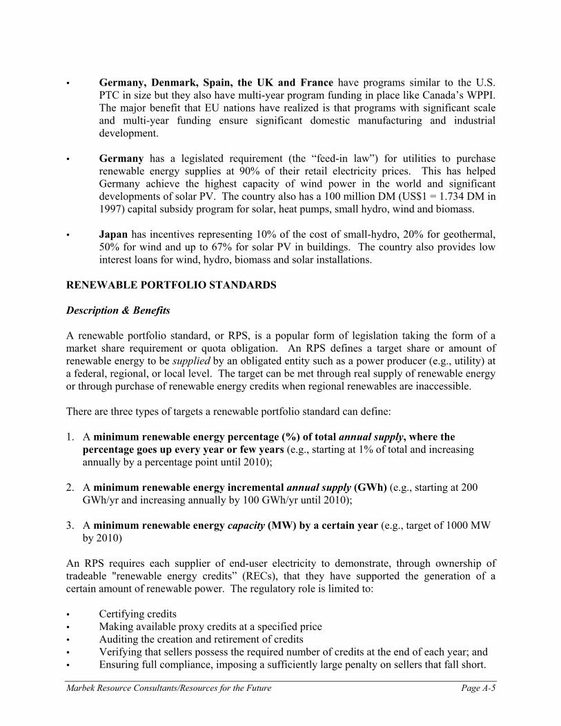
Marbek Resource Consultants/Resources for the Future Page A-5
Germany, Denmark, Spain, the UK and France have programs similar to the U.S.
PTC in size but they also have multi-year program funding in place like Canada’s WPPI. The major benefit that EU nations have realized is that programs with significant scale and multi-year funding ensure significant domestic manufacturing and industrial development.
Germany has a legislated requirement (the “feed-in law”) for utilities to purchase renewable energy supplies at 90% of their retail electricity prices. This has helped Germany achieve the highest capacity of wind power in the world and significant developments of solar PV. The country also has a 100 million DM (US$1 = 1.734 DM in 1997) capital subsidy program for solar, heat pumps, small hydro, wind and biomass.
Japan has incentives representing 10% of the cost of small-hydro, 20% for geothermal, 50% for wind and up to 67% for solar PV in buildings. The country also provides low interest loans for wind, hydro, biomass and solar installations.
RENEWABLE PORTFOLIO STANDARDS Description & Benefits A renewable portfolio standard, or RPS, is a popular form of legislation taking the form of a market share requirement or quota obligation. An RPS defines a target share or amount of renewable energy to be supplied by an obligated entity such as a power producer (e.g., utility) at a federal, regional, or local level. The target can be met through real supply of renewable energy or through purchase of renewable energy credits when regional renewables are inaccessible. There are three types of targets a renewable portfolio standard can define: 1. A minimum renewable energy percentage (%) of total annual supply, where the
percentage goes up every year or few years (e.g., starting at 1% of total and increasing annually by a percentage point until 2010);
2. A minimum renewable energy incremental annual supply (GWh) (e.g., starting at 200
GWh/yr and increasing annually by 100 GWh/yr until 2010); 3. A minimum renewable energy capacity (MW) by a certain year (e.g., target of 1000 MW
by 2010) An RPS requires each supplier of end-user electricity to demonstrate, through ownership of tradeable "renewable energy credits” (RECs), that they have supported the generation of a certain amount of renewable power. The regulatory role is limited to:
Certifying credits Making available proxy credits at a specified price Auditing the creation and retirement of credits Verifying that sellers possess the required number of credits at the end of each year; and Ensuring full compliance, imposing a sufficiently large penalty on sellers that fall short.

Marbek Resource Consultants/Resources for the Future Page A-6
A renewable procurement target is similar to an RPS, except is usually internally defined by a large organization such as a federal, provincial, or municipal government. This procurement target sets a goal to purchase a certain share or amount of the organization’s total annual electricity from renewable sources. Renewable procurement targets can also be defined in three ways, similar to the RPS types above, except for electricity consumed rather than supplied. Also similar to an RPS, a procurement target can be met through real consumption of renewable energy or through purchase of renewable energy credits when regional renewables are inaccessible. Some benefits of RPS legislation are that they: Help utilities prepare for future annual obligations well in advance Work well with financial incentives including penalties for non-compliance Help consumers get the best price for renewable electricity since a renewable electricity
market is created with competition between generators bidding to meet the utility's obligations
Use industry-friendly mechanisms to diversify energy markets Foster fair competition and market stability Spark economic development, especially in rural areas Are competitively neutral since they apply equally to all sellers; and Do not require the centralized collection and dissemination of funds or require
Government agencies to make decisions about winners and losers. The market decides which renewable plants to build, where, and for what price.
Current Canadian Situation Although no national RPS is planned for Canada, a federal-provincial working group is currently examining how renewable portfolio standards could work in the Canadian context (considering that utilities are under provincial jurisdiction). As an unlegislated measure, Canada’s 2002 federal Climate Change Plan set a minimum renewable procurement target of 10% (3.9 Mt) of new electricity-generating capacity in Canada – if implemented, it would be the strongest federal procurement program in North America. This plan suggested the following to help achieve the federal goal: Expanded production incentives Renewable energy portfolio standards in provinces Increased efforts to develop market demand Proposed emissions trading system Encouraged voluntary purchase of green power by consumers; and A proposed electricity-labelling scheme indicating the relative environmental impact of
different electricity-generating sources. Although no Canadian provincial portfolio standards have been legislated yet, following is a progress summary on provincial RPSs and defined procurement targets:

Marbek Resource Consultants/Resources for the Future Page A-7
BC – In 2002, BC proposed 50% of all new capacity from “B.C. Clean Electricity” by 2012 as a voluntary goal with no legislation behind it. The broad definition for the 50% includes efficiency improvements at existing facilities, co-generation of heat and power, and all low-impact renewable energy technologies. Possible rate increases of 0.1-0.2% over the next decade are expected. Policies such as net metering and interconnection standards will be developed to support the goal.
AB – In 2002, AB proposed 3.75% renewables capacity (~600 MW new capacity) by 2008 with no legislative action pending. The following efforts will assist with reaching this goal: 1) emissions intensity of electricity supplied to consumers will be reported by electricity retailers; 2) at least 25% of electricity consumed at government facilities will be generated from green power sources in 2004; and 3) the government will continue to support the development of green corridors, thus promoting increased use of alternative fuel vehicles.
ON – In 2002, ON proposed 10% renewables by 2010 with legislature expected to act in Spring 2004. The following efforts will assist with reaching this goal: 1) provincial government commitment to purchase 20% of its electricity from green sources; and 2) all newly constructed government buildings will also use energy efficient or clean sources of energy. The probable impact of Ontario’s proposed RPS on blended wholesale prices is < 1% for the first years and < 2% by 2010.
QC - The provincial regulator, Regie de l’Energie, has called for a wind resource commitment of 50 MW per year for seven years, making the total installed capacity 450 MW.
NB – In 2002, New Brunswick declared it will implement an RPS.
NS – According to the Nova Scotia Energy Strategy Progress Report II (2004), NS created a short-term (3-year) voluntary renewable energy target starting in December 2001 for new IPPs totalling 2.5% of provincial generation capacity, or approximately 50 MW. The Electricity Marketplace Governance Committee (EMGC) of NS has now recommended an RPS to begin in 2006. A small green-power premium will likely be applied to the electricity rates of all NS electricity consumers. Current estimates indicate such an increase would likely occur in 3-5 years and be less than 0.5-1%.
PE – PEI has proposed 10% renewables by 2010. Lastly, in terms of green procurement, the Canadian government has purchased green power from utilities in Alberta, Saskatchewan (25,000 MWh for $12.4 million), and PEI (13,000 MWh for $4.5 million). A number of municipalities currently have renewable procurement targets: Calgary, AB – Calgary’s transit authority recently signed a commitment to purchase
21,000 MWh/yr of wind-generated electricity from a local independent power producer, Vision Quest Wind Electric, for the next 10 years. Calgary is the first city in North America to offer users a green powered public transit system.

Marbek Resource Consultants/Resources for the Future Page A-8
Greater Vancouver Regional District (GVRD), BC - In 2002, the GVRD, along with the following municipalities, agreed to purchase green power from BC Hydro under the pilot Green Power Certificates Program:
Capital Regional District (Victoria) Building Services Group Corporation of the City of White Rock; and Resort Municipality of Whistler.
Alberta Urban Municipalities Association – This group made a formal Commitment
ensuring that 2% of power needs of municipalities participating in the electric aggregation initiative are obtained through green procurement.
Foreign Experience Renewable portfolio standards are credited for some of the most significant renewable energy success stories in the United States, resulting in low-cost wind power proliferating in Texas and promising solar generation in Arizona. Seventeen U.S. states have set RPS or similar goals for encouraging renewable power generation; of those, the standards most widely studied are: California - In 2002, California became legislated to generate 20% of its electricity from
renewable energy no later than 2017 by increasing the supply of renewable power by 1% per year from the current 10% - the most stringent RPS to date in the U.S., although a smaller leap for a state which already has a viable renewable energy market.
Texas - The Texas renewable energy mandate of 1999 requires utilities to acquire 400 megawatts (MW) of new generating capacity from renewable technologies by 2003; increasing to 850 MW by 2005, 1,400 MW by 2007, and 2,000 MW by 2009 (equal to 3% of total capacity). The Texas RPS, combined with the US Federal Production Tax Credit, resulted in the construction of more than ten wind projects in the first year with a combined new generating capacity of 1,200 MW. This new capacity far exceeds the 2005 target, according to the Electric Reliability Council of Texas, and is ahead of every other US state for the same period. Texas also has an accessible wind resource, which helps tremendously. Highlights of the Texas RPS include:
Ease of administration Allowance for renewable energy credit trading Requirement for all retailers to disclose where their electricity comes from Allowance for net metering Robust tracking system Adequate enforcement through penalties.
Arizona - Arizona is building toward an RPS of 1.1% in 2007 with 60% of that from
solar sources, which are plentiful in the state. July 2003 results include 5 MW of PV, according to a report by Arizona’s Cost Evaluation Working Group.
Nevada - Nevada's RPS, signed in 2001, requires the total renewable electricity supplied in the state to increase from 5% in 2003 to 15% in 2013 by 2% increments every two

Marbek Resource Consultants/Resources for the Future Page A-9
years. It also allows the Nevada Public Utilities Commission to develop a trading mechanism for renewable energy credits for the state's utilities.
Other foreign RPS legislation includes: The United Kingdom previously established renewable procurement targets for
electricity suppliers but have now adopted a portfolio standard approach;
Denmark requires a minimum amount of biomass to be used in coal-fired plants and has a national RPS; and
Australia has legislated an RPS of 2% by 2010.

APPENDIX B
Overview of the Model
From: Fischer, Carolyn and Richard G. Newell. “Environmental and Technology Policies for Climate Change and Renewable Energy.” RFF Discussion Paper 04-05, April 2004.

Marbek Resource Consultants/Resources for the Future Page B-1
We develop a unified framework to assess the six different policy options for reducing greenhouse gas emissions and promoting the development and diffusion of renewable energy. The stylized model is deliberately kept simple to highlight key features. It includes two sectors, one emitting and one non-emitting, and both are assumed to be perfectly competitive and supplying an identical product, electricity. Fossil fuel production is assumed to be the marginal technology, setting the overall market price; thus, to the extent that renewable energy is competitive, it displaces fossil fuel generation. The model has two stages: electricity generation, consumption, and emissions occur in both, while investment in knowledge takes place in the first stage and through technological change lowers the cost of renewable generation in the second. An important assumption is that firms take not only current prices as given, but they also take prices in the second stage as given, having rational expectations about those prices. To allow for consideration of the length of time it takes for innovation to occur, and for the lifetime of the new technologies, let the first and second stages be made up of n and m years, respectively. For simplicity, we assume that no discounting occurs within the first stage; this assures that behavior within that stage remains identical. However, let δ represent the discount factor between stages. It is possible to allow for discounting in the second stage by altering m to reflect such discounting; in that case m can be thought of as “effective” years. Emitting Fossil Fuels Sector The emitting sector of the generation industry relies on fossil fuels and is denoted with superscript F. Total output from the emitting sector is tf in year t. Marginal production costs MC are assumed to be constant with respect to output and weakly decreasing in emissions intensity tµ , up to some natural rate, 0µ . This form allows for a tradeoff between emissions intensity and higher costs (i.e., a carbon abatement cost function). Two policies affect the fossil fuel sector directly: an emissions price and an output tax (which may be explicit or implicit, as with the portfolio standard discussed below). Let tτ be the price of emissions (i.e., emissions tax or equilibrium permit price) and tφ be the tax on fossil fuel generation at time t, respectively. Other policies that stipulate quantity standards, such as renewable portfolio standards and emission performance standards, will be specified in the next section, as they require some modifications to the generalized model. Profits for the representative emitting firm are: 1 1 1 1 1 1 2 2 2 2 2 2( ( ) ) ( ( ) )F n P MC f m P MC fπ µ τ µ φ δ µ τ µ φ= − − − + − − − , (1) where Pt is the price of electricity. The firm maximizes profits with respect to output and emissions intensity, yielding the following first-order conditions:
0 : '( ) ;F
t tt
MCπ µ τµ
∂= − =
∂ (2)

Marbek Resource Consultants/Resources for the Future Page B-2
0 : ( ) .F
t t t t tt
P MCfπ µ τ µ φ∂
= = + +∂ (3)
Thus, as shown in equation (2), the price of emissions (τ) determines the emission rate. The corresponding marginal costs of output are then constant (including the output tax (φ ) and the price of the emissions embodied in that output (τµ )). Thus, the fossil fuel sector is the “marginal technology”—as long as fossil fuel generation occurs, the competitive market price must equal the sum of these marginal costs, as shown by equation (3).35 Total emissions, tE , are the product of the emission rate and fossil fuel output:
t t tE fµ= . (4)
In the absence of a price on emissions, the first-order condition for emission intensity implies
'( ) 0tMC µ− = . Let the solution to this equation be 0µ , the baseline emission rate, and the corresponding baseline price of electricity generation be 0P , where 0 0( )P MC µ= . The Non-Emitting Renewable Energy Sector Another sector of the industry generates without emissions by using renewable resources (wind, for example); it is denoted with superscript R. Annual output from the renewables sector is tq . The costs of production ( , )t tG K q are assumed to be increasing and convex in output, and declining and convex its own knowledge stock tK , so that 0qG > , 0qqG > , 0KG < , and
0KKG > , where lettered subscripts denote derivatives with respect to the subscripted variable.36 Furthermore, since marginal costs are declining in knowledge and the cross-partials are symmetric, 0qK KqG G= < . Note that we have simplified considerably by assuming there is technological change in the relatively immature renewable energy technologies, but none in the relatively mature fossil fuel technologies. While it is of course not strictly true that fossil fuel technologies will experience no further technological advance, incorporation of a positive, but slower relative rate of advance in fossil fuels would complicate the analysis without adding substantial additional insights.
35 The assumption of a single fossil energy technology is admittedly strong and requires some caveats. As long as the marginal technology exhibits constant marginal costs, the equilibrium effects on the market price and surplus are the same. The exceptions involve policies with an emissions price when emissions intensities vary across fossil technologies. For example, if coal is used by the inframarginal technology and natural gas turbines are the marginal technology, an emissions price will raise costs more for coal, but the market price will only reflect the cost increase for natural gas (unless coal becomes no longer inframarginal), implying a loss of producer surplus for coal. Policy effects on average emissions intensity will also vary, and those without an emissions price will tend to displace the lower-emitting marginal technology. We feel that this simplification allows us to capture the key qualitative results; a richer modelling is only likely to exacerbate the welfare differences of the policies. 36 Longer-term convexity of the renewable cost function is attributable to decreasing quality of available land for wind and biomass generation. Input scarcity is not a substantial longer-term issue for fossil-based production, however, justifying the simplifying assumption of constant marginal costs (i.e., constant returns to scale).

Marbek Resource Consultants/Resources for the Future Page B-3
The knowledge stock ( , )t tK H Q is a function of cumulative R&D, Ht, and of cumulative experience through “learning by doing” (LBD), tQ , where 0HK ≥ and 0QK ≥ , and
QH HQK K= . Cumulative R&D increases in proportion to annual investment in each stage, th , so 2 1 1H H nh= + . Cumulative experience increases with total output during the first stage, so
2 1 1Q Q nq= + . Research expenditures, ( )tR h , are increasing and convex in the amount of new R&D knowledge generated in any one year, with ( ) 0hR h > for h > 0 , (0) 0hR = , and 0hhR > . An important issue is whether research and experience are substitutes, in which case 0HQK < , or complements, in which case 0HQK > . Two price-based policies are directly targeted at renewable energy: a renewable energy production subsidy (s), and a renewable technology R&D subsidy in which the government offsets a share (σ) of research expenditures. In our two-stage model, profits for the representative non-emitting firm are: ( )( )1 1 1 1 1 1 2 2 2 2 2( ) ( , ) (1 ) (( ) ( , ))R n P s q G K q R h m P s q G K qπ σ δ= + − − − + + − , (5) where: 2 2 2( , )K K H Q= . The firm maximizes profits with respect to output in each stage and R&D investment, yielding the following first-order conditions:
( )
( )1
1 1 1 1 2 2 2 2
2 2 2 22
1 2 2 2 21
( , ) ( , ) ( , ) 0;
( , ) 0;
(1 ) ( ) ( , ) ( , ) 0.
R
q K Q
R
q
R
h K H
n P s G K q mG K q nK H Qq
m P s G K qq
n R h mG K q nK H Qh
π δ
π δ
π σ δ
∂= + − − =
∂
∂= + − =
∂
∂= − − − =
∂
Rearranging, we get:
1 1 1 1 2 2 2 2( , ) ( , ) ( , );q K QG K q P s mG K q K H Qδ= + − (6)
2 2 2 2( , ) ;qG K q P s= + (7)
1 2 2 2 2(1 ) ( ) ( , ) ( , ).h K HR h mG K q K H Qσ δ− = − (8) As shown in equation (6), the renewable energy sector produces until the marginal cost of production equals the value it receives from additional output, including the market price, any production subsidy, and the contribution of such output to future cost reduction through learning-

Marbek Resource Consultants/Resources for the Future Page B-4
by-doing (note that the last term in equation (6) is positive overall).37 Second stage output does not generate a learning benefit, so there is no related term in equation (7). Meanwhile, as shown in equation (8), the firm also invests in research until the discounted returns from R&D equal investment costs on the margin. Consumer demand Renewable energy generation and fossil fuel production are assumed to be perfect substitutes. Let ( )C P be the consumer demand for electricity, a function of the price, where '( ) 0C P < . In equilibrium, total consumption must equal total supply, the sum of fossil fuel and renewable energy generation: ( )t t tC P f q= + . In this model, fossil fuels are the marginal technology (by the assumption of flat marginal costs), and their generation costs determine the price of electricity. Fossil fuel output is therefore equal to the residual after profitable renewable energy is produced: ( )t t tf C P q= − . Thus, any increase in renewable energy production “crowds out” fossil fuel production.
Consumer surplus is therefore ( )tP
CS C P dP∞
= ∫ . Thus, the change in consumer surplus due to
the renewable energy policy in this partial equilibrium model is:
1 2
0 0
( ) ( ) .P P
P P
CS n C P dP m C P dPδ
∆ = − −
∫ ∫ (9)
Welfare Policies also have implications for government revenues, which we denote as V. We assume that these revenues are raised or returned in a lump-sum fashion. The change in these transfers equal the tax revenues net of the cost of the subsidies: ( ) ( )1 1 1 1 1 1 1 2 2 2 2 2 2( ) ( ) ( )V n f s q R h m f s qφ τ µ σ δ φ τ µ∆ = + − − + + − (10) Environmental damages are a function of the annual emissions and the length of each stage. To be able to accommodate both for flow and stock pollutants, we write this function in a general form: 1 2 0 0( , , , ) ( , , , )D D E E n m D E E n m∆ = − (11)
37 Note therefore that we are assuming here that firms have perfect foresight, that there are no knowledge spillovers, and that firms internalize any future returns to investments in R&D and LBD. For the present purposes we also assume that the costs of R&D and LBD are fully reflected in the market prices faced in making these investments. These assumptions are not meant to necessarily reflect reality, but rather to model a simplified situation upon which intuition can be developed and further modelling extensions can be built.

Marbek Resource Consultants/Resources for the Future Page B-5
The change in welfare due to a policy is the sum of the changes in consumer and producer surplus, net of the change in environmental damages and revenue transfers from the subsidy or tax: .RW CS D Vπ∆ = ∆ + ∆ −∆ + ∆ (12) Note that constant marginal costs in the fossil fuels sector implies zero profits, so 0Fπ∆ = . However, welfare is unlikely to be the only metric for evaluating policy. Other indicators may be total emissions, consumer surplus, renewable energy market share, and so on. General equilibrium factors—like interactions with tax distortions, leakage, or other market failures—can also be important for determining welfare impacts. Political economy constraints may also be important for determining policy goals. To the extent that these unmodeled issues are present, this partial equilibrium presentation of welfare within the sector will not reflect the full social impacts; still, it represents a useful baseline metric. Response of renewable energy to changes in prices, output, and R&D While policies can affect both the market price of energy and the renewable energy subsidy, the renewable energy producer ultimately cares about the total price it receives for generation in each period, which we define as:
.Rt t tP P s≡ + (13)
The Appendix derives the comparative statistics for the response of the renewable energy sector to changes in these prices and in the price it pays for research. The main results are as follows. First, renewable energy output in each period is increasing with the price received in that period. (i.e., / 0R
t tdq dP > .) Output in the second stage is also increasing in knowledge, since marginal costs are lowered ( / 0t tdq dK > ). Next, R&D is increasing in the second-stage price, since higher prices imply more renewable output, which implies more scope for profits from reduced costs. Similarly, to the extent there is learning by doing, first-stage output is increasing in the second-stage price, for the same reasons. Unsurprisingly, R&D is also increasing in its own subsidy, since effective investment costs to the firm decrease. The harder questions regard how first-stage output responds to R&D, and vice-versa—in other words, how LBD and R&D interact. While both are increasing in second-stage output, the incidence across the two forms of knowledge accumulation depends on the degree of their substitutability or complementarity. That substitutability also determines whether they respond in the same or opposite directions due to changes in the first-stage price and in the R&D subsidy, since those changes affect the relative prices of LBD and R&D. If R&D and LBD are complements, first-stage production will tend to increase with investment in R&D. That means an increase in the R&D subsidy will also increase first-stage renewable generation. Similarly, an increase in first-stage renewable energy prices can also increase R&D, if it is complemented by more LBD.

Marbek Resource Consultants/Resources for the Future Page B-6
On the other hand, if R&D and LBD are substitutes in knowledge production, then more R&D makes LBD less productive, given any output level. But the increase in second-stage output resulting from lower costs due to more R&D also tends to make LBD more valuable. First-stage production may then increase or decrease with investment in R&D. But a strong substitution effect means that a larger R&D subsidy will decrease first-stage production, and a larger subsidy to first-stage production will decrease R&D investment, as R&D and LBD crowd each other out. These interactions will be important determinants of policy effects, since different policies have different implications for the prices of output in the first and second stages and the cost of R&D. Policy Scenarios As developed in the modelling section, renewable energy production depends on the price received by that sector and the cost of R&D investment. Fossil fuel energy production depends on the amount of renewable sector output and the price of electricity, and emissions intensity depends on the price of emissions. Different policies vary in their effects on these different prices, resulting in different market equilibria. As we will see, the policies therefore provide varying incentives for emissions reduction along these different margins—emissions intensity, energy conservation, and renewable energy output—leading to a divergence in their relative efficiency. No policy We have defined 0µ as the baseline emissions rate and 0P as the baseline electricity price, so in the absence of policy (i.e., 1 0t tsφ τ σ= = = = ), the first-order conditions for production imply that output prices equal this baseline price in both markets and over time: 0
Rt tP P P= = . We
assume that an interior solution exists; that is, that some wind energy is viable without any policy. A sufficient condition would be that 1 0( ,0)qG K P< . However, wind production could occur even if marginal production costs are higher than the price in the first stage, as long as the value of learning-by-doing for lowering second-stage costs is sufficient. Fixed-price policies We look first at three policies that directly set prices: an emissions price, a renewable production subsidy, and a tax on fossil-based production. Emissions price With a direct price for emissions—via either an emissions tax or a tradable emissions permit system—the fossil fuel sector has an incentive to lower its emission rate until the marginal cost of reduction equals the emissions price '( )t tMC µ τ− = . The market price of electricity reflects the total marginal cost of fossil generation, inclusive of the embodied emissions cost as well as higher marginal production costs: ( )t t t tP MC µ τ µ= + (see equation (3)). Without other subsidies, the renewables sector receives the market price for electricity ( R
t tP P= ), and the price increase promotes greater renewable energy generation in both stages. The prospect of more output in the second stage increases knowledge investment incentives in the renewable sector, both for R&D

Marbek Resource Consultants/Resources for the Future Page B-7
and learning. The higher market price also means consumers have added incentive to conserve. Thus, the emissions price provides efficient incentives for achieving a given emissions reduction goal as it provides equalized incentives for emission reduction along all three margins—emissions intensity, output reduction (via price increase), and renewable energy production. Renewable energy production subsidy Under a renewable production subsidy, since there is no direct price on emissions, there is no reduction in fossil emissions intensity, and 0tP P= , as in the no-policy scenario. While the market price of electricity remains unchanged, and thus provides no incentive for energy conservation, the effective price received by the renewable energy sector rises by the amount of the subsidy, so that 0
Rt tP P s= + . In this way, the renewables subsidy crowds out fossil fuels
generation in both stages and reduces emissions. Fossil fuel production tax The analytic structure of a fossil fuel production tax is similar to the renewables subsidy, except that it is a rise in the consumer price of electricity, rather than a direct subsidy, that raises the price received by renewables. Thus, both the market price and the effective price received by the renewable energy sector rise by the amount of the tax: 0
Rt t tP P P φ= = + . Although no incentive
exists to reduce emissions intensity, to the extent that demand falls due to higher prices, fossil output and emissions will be lower than under an equivalent renewable energy subsidy. Renewable energy technology R&D subsidy Without a price on emissions or subsidy/tax on output, output prices in both markets equal the baseline price ( 0
Rt tP P P= = ). The primary effect of the R&D subsidy is to increase research
expenditures and lower future renewable costs, crowding out some fossil fuels generation in the second stage. The R&D policy provides no incentive for reduction in fossil emissions intensity or energy conservation through an electricity price increase. Regarding incentives for technological change, in the appendix we show that an increase in R&D can encourage learning either by making it more productive if R&D and learning are complements, or by inducing a sufficient expansion in second-stage output. On the other hand, if they are substitutes R&D could discourage learning. In the latter case, although an R&D subsidy would increase renewable energy generation in the second stage, renewable output will be lower in the first stage relative to the baseline. The time path of emissions would tilt in the opposite direction, rising in the first stage and falling in the second. In the absence of a learning effect ( 0QK = ), the R&D subsidy would do nothing for first stage emissions.

Marbek Resource Consultants/Resources for the Future Page B-8
Rate-based policies Two additional, rate-based policies familiar to the electricity generation sector are portfolio standards and tradable performance standards. A portfolio standard requires a certain percentage of generation to come from renewable energy sources. A tradable performance standard mandates that average emissions intensity of all generation not exceed a standard. Both policies create effective taxes on fossil fuel generation and subsidies for renewable energy sources. However, those prices are not fixed, like in the previous policies, but rather adjust endogenously according to market conditions to achieve the targeted rate. Endogenous prices raise additional issues with respect to innovation incentives. Essentially, as increased knowledge brings down the costs of renewable energy, the standards become less costly to meet, which becomes reflected in the implicit taxes and subsidies. The question is how the renewable energy sector perceives these price changes. Do they recognize the impact of their innovation decisions on second-stage prices? Do they myopically expect prices to remain unchanged? Or do they expect the future prices, but take them as given, as competitive firms? Given our starting assumptions of a representative, perfectly competitive firm, we will proceed with the latter assumption. This view is most appropriate for describing firm-specific innovation in a sector of many small, competitive firms. These assumptions may be strong, and exploring alternatives will be an important extension, in particular to incorporate spillover effects. A long literature recognizes the differences in incentives depending on the structure of markets for output and for innovation.38 But one must begin somewhere, so we examine the logical starting point of price-taking firms with rational expectations. Renewable energy portfolio standard We model the portfolio standard as a requirement that α % of generation be from renewable energy sources in each stage (i.e., no banking allowed). We assume that responsibility lies with the emitting industry to satisfy the portfolio constraint. Thus, the fossil fuel producer must purchase or otherwise ensure at least α units of renewable energy for every (1 )α− units of fossil fuel generation, or /(1 )α α− “green certificates” for every unit generated. In equilibrium, the incentives correspond to a combination of the fossil fuel production tax and renewable energy subsidy cases. Assuming this constraint binds, the renewable energy sector receives a subsidy per unit output equal to the price of a green certificate, t̂s , where “^” denotes equilibrium values under the portfolio standard. The effective tax per unit of fossil-fueled output under this policy, t̂φ , is then proportional to the effective subsidy to the renewable energy producer:
ˆ ˆ1t tsαφ
α=
−. (14)
38 See e.g., Milliman and Prince (1989), Biglaiser and Horrowitz (1995), Jung et al. (1996), Fischer et al. (2003), Requate and Unold (2002). Dynamic problems are also treated in Petrakis et al. (1999) and Kennedy and Laplante (1999).

Marbek Resource Consultants/Resources for the Future Page B-9
The implicit tax and subsidy are determined competitively by the market to meet the portfolio constraint. The resulting market price of electricity is 0 ˆ /(1 )t tP P sα α= + − , while the price received by the renewables sector is 0ˆ ˆ /(1 )R
t t t tP P s P s α= + = + − . The portfolio standard provides no incentive to lower the emissions intensity of fossil fuels, but crowds out fossil fuel generation by implicitly taxing it and subsidizing renewables compared to the market price. The rise in consumer prices is positive (unlike a pure renewables subsidy where it is zero), but only a fraction of the rise in the effective price received by renewables (whereas a fossil energy tax would fully pass this increase on to consumers). Thus the portfolio standard results in only modest energy conservation incentives. Another important difference is that, if the portfolio standard is fixed as we have assumed, the implicit tax and subsidy decline over time as renewable energy costs fall due to technological change. This occurs because the implicit tax/subsidies reflect the shadow cost of meeting the renewable production constraint, and this shadow cost declines as the cost of renewable production declines. Emission performance standard While a portfolio standard requires a certain percentage of renewable energy, a performance standard requires an average emissions intensity of all generation. With a tradable performance standard of µ , the emitting firm must buy emission permits to the extent that its emission rate exceeds that standard. The price of emissions at time t, tτ% , will now be determined by a market equilibrium, denoted by “~”. All firms are in effect allocated µ permits per unit of output, which leads to an implicit subsidy of tτ µ% per unit of output. Thus, if the standard is binding, the fossil fuel sector will be a buyer of permits costing ( )t tτ µ µ−% per unit of output, and the renewable sector will be a seller of permits valued at tτ µ% per unit of output. Thus, the emissions performance standard corresponds to a combination of an emissions price tτ% and a generation subsidy for both renewable and fossil energy producers, where
.t t ts τ µ φ= = − %% % (15) The equilibrium values are determined in conjunction with the previous market-clearing conditions for energy supply and demand, along with the additional constraint that
( )t t t tf q fµ µ≤ + . (16)
The resulting market price of electricity is ( ) ( ) ( )t t t t t t t tP MC MCµ τ µ φ µ τ µ µ= + + = + −%% % , reflecting both the higher cost of achieving lower emissions intensity, and the cost to fossil fuel producers of emissions in excess of the standard. The price received by the renewables sector is
( )Rt t t t tP P s MC µ τ µ= + = +% % , which also includes the revenues they gain from permit sales (i.e.,
the implicit subsidy). Note that the price received by renewables is the same as with an equivalent pure emissions price (i.e., if t tτ τ= % ), assuring the same amount of renewable energy. The incentive to lower emissions intensity is also the same for the fossil fuel sector in that case. However, the consumer

Marbek Resource Consultants/Resources for the Future Page B-10
price is lower by the output subsidy, tτ µ% , and the resulting larger total output is filled by additional fossil fuel generation, meaning that total emissions are higher. As with the portfolio standard, a fixed performance standard implies a subsidy that changes over time. In this case, as costs fall in the second stage, the expansion of renewable energy allows fossil fuel sector emissions to increase. Some of this will arise from greater production, and some from increased emissions intensity, as the permit price falls.

APPENDIX C
References, Assumptions and Notes on Grid-Power RET Resources

Marbek Resource Consultants/Resources for the Future Page C-1
Assumptions and Notes for Installed Capacity Grid-Power
RET Source for Capacity Notes
Wind Ref 4 Current installations shown on CanWEA website Hydro Ref 13 Includes many existing small hydro site which may NOT be EcoLogo-certifiable. Solar PV Ref 1 LFG Ref 3 Biomass Ref 3, p 119 Many of the existing 1900 MW of biogas plants are NOT EcoLogo-certifiable and
are off-grid such as for pulp and paper industry plants. Only 128 MW used by independent power producers.
Wave Ref 11 Plans for 4MW wave generator off BC fell through Tidal Ref 3 20 MW quoted in reference for NS tidal generator, but not EcoLogo-certifiable so
not counted Geothermal Ref 5

Marbek Resource Consultants/Resources for the Future Page C-2
Assumptions and Notes for Estimating Technical Potential
Source for Grid-Power RET
Capacity factor
Low potential
High potential
Notes
Wind Ref 1 Ref 13 Ref 14 Offshore wind is not considered in the estimate as data is largely non-existent (Ref 20). Even though turbines in Canada are typically 25-35% capacity factor today, 35% was chosen from PP 2002 paper since higher and larger turbines are expected in the future
Hydro Ref 13 Ref 6 Ref 18 Ref 18 notes: “based on EcoLogo: larger than 11,000 MW, assuming that most existing sites smaller than 20 MW can be exploited in a fashion that complies with EcoLogo requirements, and that there are several more sites that are larger than 20 MW for which one could assume the same. We know that at least 3,000 MW more than identified in the Atlas exist in Canada, based on local assessments”
Solar PV Ref 3, pp 113-121
Ref 2 Ref 22 CanSIA representative indicated that total potential cited by Pollution Probe (9,785 MW) is very low – recommended using 70,000 MW as a minimum with no maximum supplied. Therefore, use PP estimate as low value, and 100,000 as high (number chosen in the absence of others supplied).
LFG Ref 3, pp 113-121
Ref 16 Ref 3, pp 113-121
Conestoga Rovers and Associates (CRA): “Although all landfills produce methane, there is a certain threshold LFG production rate that the landfill has to produce to make capture and utilisation an economically viable proposition.”
Biomass Ref 3, pp 113-121
Ref 3, pp 113-121
Ref 12, p 10
High: BIOCAP estimates 2 EJ/yr available biomass energy
Wave Ref 11 Ref 11 Ref 11 Tidal Ref 1 Ref 11 Ref 3 PP notes: “at a 30% capacity factor, 1 TW of wave power could provide five times the electricity
Canada consumes in a year (about 600 TWh).” Geothermal Ref 5 Ref 5

Marbek Resource Consultants/Resources for the Future Page C-3
Assumptions and Notes for Estimating Practical Potential
Source for Grid-Power RET 2010 -
Low 2010 - High
2020 - Low
2020 - High
Notes
Wind Ref 3, pp 113-121
Ref 4 Ref3 Ref 20 CanWEA: “… it is clear that electricity grids can handle at least 20% penetration by intermittent renewable energy sources at a reasonable cost (approx. 45,000 MW of wind). Canada has the wind resource to do this, but we still have to assess if it is "practical" from a transmission standpoint.” Off-shore wind not included because currently no estimates exist from independent sources. The best available estimate is 2,500 MW of economically feasible off-shore wind power, consisting of 500 MW on each coast and 1,500 MW on the Great Lakes; source: O’Gorman, Steve; Canadian Hydro Developers response to extracts from Pollution Probe Green Power Workshop Backgrounder document for Feb 2004 workshop.
Hydro Ref 18 Ref 13 Ref 18 Reference 18 notes: Feasible by 2010: 5,600 MW (= 40% of total; includes projects already in the pipeline) Feasible by 2020: 9,800 MW (= 70% of total)
Solar PV Ref 22 Ref 21 Ref 3, pp 113-121
Ref 22 CanSIA notes: “PV has likely gone as far as it can in significant increases in deployment in "off grid" markets in Canada. International, industrialized country markets are now 90% grid and 10% off grid - we would expect Canada to follow international trends. PV is installed on building roofs and hence the criteria on distance to transmission lines is irrelevant - the limitations relate to the surface area of buildings that have adequate exposure to solar energy… should not be a limiting factor. CanSIA estimates that the industry can sustain 35-40% annual growth without putting a strain on its infrastructure”
LFG Ref 3, pp 113-121
Ref 3, pp 113-121
Environment Canada agrees with PP 2002 numbers as being double and triple today’s installed capacity
Biomass Ref 23 Ref 23 Ref 3, pp 113-121
Most biomass is waste from industrial processes and most technical studies do not differentiate well the breakdown of biomass into grid-connected and off-grid (on-site use for other industrial processes). Maximums assume aggressive use of residual biomass from agricultural and other industries, even though some, especially agriculture, need to recycle biomass back into the soil to preserve nutrients for future crop growth. PP later clarified that 1500-2000 MW could be possible for 2010. High est. was used instead of previous low of 6000 MW.
Wave Ref 23 Ref 23 Ref 23 PP said still experimental and no utility-sized plants until after 2020 so maybe only a pilot plant before then Tidal Ref 23 Ref 23 Ref 23 Ref 23 PP said maybe a pilot by 2010 then increasing by maybe 50 MW or more by 2020 Geothermal Ref 19 Ref 3,
pp 113-121
Ref 3, pp 113-121
Only BC has hot enough geothermal potential to tap into for electricity generation. Only two companies found were looking at this generation: Western Geopower and North Pacific Geopower. Both companies recognised finite potential that could be harnessed using technology available in the near future.