ÉCOLE DE TECHNOLOGIE SUPÉRIEURE

UNIVERSITÉ DU QUÉBEC

THESIS PRESENTED TO ÉCOLE DE TECHNOLOGIE SUPÉRIEURE

IN PARTIAL FULFILLMENT OF THE REQUIREMENTS FOR A MASTER’S DEGREE WITH THESIS IN MECHANICAL ENGINERING

M.A.Sc.

BY Nila ABOLFATHI NOBARI

BAYESIAN UPDATING OF HYDROELECTRIC TURBINE FATIGUE RELIABILITY

MONTREAL, FEBRUARY 02 2016

© NILA.A.NOBARI, 2016

© Copyright

Reproduction, saving or sharing of the content of this document, in whole or in part, is prohibited. A reader

who wishes to print this document or save it on any medium must first obtain the author’s permission.

BOARD OF EXAMINERS THESIS M.SC.A.

THIS THESIS HAS BEEN EVALUATED

BY THE FOLLOWING BOARD OF EXAMINERS Mr. Souheil-Antoine Tahan, ing. Ph.D., Thesis Supervisor Mechanical Department at École de technologie supérieure Mr. Martin Gagnon, ing. Ph.D., Thesis Co-supervisor Institut de rehcerche d’Hydro-Québec (IREQ) Mr. Jean-Pierre Kenné, ing. Ph.D., Chair, Board of Examiners Mechanical Department at École de technologie supérieure Mr. Michel Rioux, ing. Ph.D., Member of the jury Automated Manufacturing Engineering Department at École de technologie supérieure

THIS THESIS WAS PRENSENTED AND DEFENDED

IN THE PRESENCE OF A BOARD OF EXAMINERS AND THE PUBLIC

JANUARY 19, 2016

AT ÉCOLE DE TECHNOLOGIE SUPÉRIEURE

BAYESIAN UPDATING OF HYDROELECTRIC TURBINE FATIGUE

RELIABILITY

Nila.A.Nobari

ABSTRACT

In fatigue design, uncertainties that exist in material, environment, and loading could arise due to manufacturing processes and changing with environment condition. Therefore because of the lack of information and cost of inspection, updating the fatigue model variables to decrease the uncertainties is necessary. In this study, Paris model is used to model the crack growth rate for hydroelectric turbine runner. We applied the Bayesian method to construct the posterior distribution. After constructing the posterior distribution, we update it by Bayesian updating approach. This method is one of the useful methods to decrease the uncertainty of variables at each loading cycle to construct precise prior distribution. The results of updating applied to Kitagawa-Takahashi limit state diagram. After modeling the proper limit state, we apply First Order Reliability Method (FORM) and Monte-Carlo Simulation (MCS) method to calculate the reliability index. In This study all of the procedures that mentioned are described, also we could see the results of effects of prior knowledge and select the distribution to analysis of reliability index. This study follows the (Gagnon, Tahan et al. 2013) research with aim of updating the fatigue reliability amount on hydroelectric turbine runner by Bayesian method.

Key-word: Bayesian methods, reliability, fatigue, hydroelectric runners.

MISE À JOUR BAYÉSIENNE DU MODÈLE DE FIABILITÉ EN FATIGUE DES ROUES HYDROÉLECTRIQUES

Nila.A.NOBARI

RÉSUMÉ

Dans une démarche de conception pour la fatigue, les incertitudes qui existent dans le matériel, l'environnement et le chargement pourraient survenir lors du processus de fabrication et de l’exploitation ce qui a pour effet une incertitude sur la vie résiduelle en fatigue. Par conséquent, en raison du manque d'informations et de coût de l'inspection, la mise à jour des variables d’un modèle de la fatigue est justifiée et nécessaire pour diminuer les incertitudes. Dans ce projet, le modèle de Paris est utilisé pour modéliser le taux de croissance de la fissure pour la roue d’une turbine hydroélectrique. Nous avons appliqué la méthode bayésienne pour construire la distribution postérieure. Après la construction de la distribution postérieure, nous mettons à jour le modèle. Cette méthode est utile pour diminuer l’influence de l'incertitude des variables à chaque cycle de chargement, ce qui permet de construire une distribution plus précise pour modéliser le comportement aléatoire des variables entrants dans le modèle de fatigue. Les résultats de la mise à jour sont appliqués à modèle d’état limite basé sur le diagramme de Kitagawa-Takahashi. Après modélisation de l'état limite approprié, nous appliquons les méthodes FORM (First Order Reliability Method) et Monte-Carlo pour calculer l'indice de fiabilité. Dans cette étude, toutes les procédures mentionnées sont décrites, aussi nous avons pu voir les résultats sur les effets des connaissances préalables sur l'indice de fiabilité. Cette étude suit la recherche démarrée par Gagnon et al. (2013) avec pour but d'actualiser l’estimation de la fiabilité par la méthode bayésienne.

Mots-clés : Méthodes bayésiennes, fiabilité, fatigue, roues hydroélectriques.

TABLE OF CONTENTS Page

INTRODUCTION .....................................................................................................................1

CHAPTER 1 STATE OF ART ..............................................................................................7

1.1 Fatigue propagation .......................................................................................................7 1.2.1 Initial crack size .................................................................................................. 8 1.2.2 Loading ............................................................................................................... 8

1.2 Reliability assessment ..................................................................................................10

CHAPTER 2 UPDATING PARAMETERS WITH BAYESIAN THEORY .......................13

2.1 Introduction ..................................................................................................................13 2.2 Data uncertainty ...........................................................................................................14 2.3 Hypothesis....................................................................................................................15 2.4 Bayesian update for fatigue variables ..........................................................................16 2.5 Results of updating variables with Bayesian theory ....................................................18 2.6 Results of updating parameters with Bayesian theory .................................................24 2.7 Conclusion: ..................................................................................................................28

CHAPTER 3 UPDATING FATIGUE RELIABILITY .......................................................29

3.1 Introduction of the structural reliability method ..........................................................29 3.2 Step 1: Identify the significant failure modes of hydroelectric turbine blades ............30 3.3 Step 2: Define probability of failure for turbine blades ...............................................30 3.4 Step 3: Construct Kitagawa-Takahashi limit state for fatigue reliability ....................32

3.4.1 Estimated reliability index for the standard normal variables .................. 34 3.4.2 Rosenblatt transformation ......................................................................... 34 3.4.3 Estimating reliability index with FORM .................................................. 35

3.5 Estimate reliability index for prior distribution ...........................................................36 3.6 Estimate reliability index for posterior distribution ....................................................38

3.6.1 Updating the posterior distribution to find the precise fatigue reliability . 39 3.7 Select target reliability index .......................................................................................44 3.8 Conclusion ...................................................................................................................44

CONCLUSION ........................................................................................................................47

RECOMANDATIONS ............................................................................................................49

APENDIX I MATLAB CODE ............................................................................................50

REFERENCES .......................................................................................................................75

LIST OF TABLES

Page Table 2.1: Amount of parameters ................................................................................16

Table 2.2: Parameter specification for crack size and stress range .............................18

Table 2.3: Conjugate pairs for prior and likelihood distribution ................................19

Table 2.4: Mean value and standard deviation for updated distribution .....................24

Table 2.5: Amount of parameters related to σΔ and a with prior and likelihood distribution .................................................................................................25

Table 3.1: Detailed results for a [mm] (Normal ( μ =1.5, σ =0.5)) ..........................36

Table 3.2: Test data (Likelihood distribution) ............................................................39

Table 3.3: Amount of prior, likelihood and updated posterior distribution ................41

Table 3.4: Reliability index and probability failure for updated distribution .............42

Table 3.5: Target reliability index ...............................................................................44

LIST OF FIGURES

Page

Figure 0.1: Schematic of Francis runner diagram (Gagnon, Tahan et al. 2013) ...........3

Figure 0.2: Probabilistic model that introduces the Kitagawa-Takahashi limit state .....4

Figure 1.1: Fatigue crack growth rate curve for metals (Ambriz, 2014) .......................9

Figure 2.1: Methodology that introduces Bayesian updating method ..........................14

Figure 2.2: Surface crack and near the surface crack ..................................................15

Figure 2.3: Prior distribution with 95% confidence interval ........................................18

Figure 2.4: Likelihood distribution..............................................................................19

Figure 2.5: Likelihood distribution and product distribution .......................................20

Figure 2.6: Prior and likelihood distribution ................................................................21

Figure 2.7: Bayesian update for crack size ...................................................................22

Figure 2.8: Bayesian update for stress range ................................................................23

Figure 2.9 : Prior probability distribution for stress range ............................................25

Figure 2.10: Likelihood probability distribution for stress range...................................26

Figure 2.11: Prior probability distribution for crack size ..............................................26

Figure 2.12 Likelihood sistribution for crack size ........................................................27

Figure 2.13: 3D of the Posterior distribution for stress range ........................................27

Figure 2.14: 3D of the Posterior distribution for crack size ...........................................28

Figure 3.1: Basic failure problem ................................................................................30

Figure 3.2: Reliability index on nonlinear limit state ...................................................32

Figure 3.3: Schematic of Kitagawa -Takahashi limit state ..........................................33

Figure 3.4: Reliability index amount ............................................................................37

Figure 3.5: Reliability index vs of crack size with MCS and FORM .........................37

XIV

Figure 3.6: Probability of failure vs crack size with MCS and FORM ........................38

Figure 3.7: Reliability index for posterior distribution with MCS ...............................39

Figure 3.8: Two updated posterior distribution for crack size .....................................40

Figure 3.9: Two updated posterior distribution for stress range ..................................41

Figure 3.10: Evolution of the probability of failure vs crack size ..................................42

Figure 3.11: Probability of failure for prior and 2th updated posterior with FORM .....43

Figure 3.12: Probability of failure for prior and 2th updated posterior with MCS ........43

Figure 3.13: Methodology to update reliability inde ………………………………….46

LIST OF ABREVIATIONS

MCS Mont Carlo simulation

FORM First order reliability method

SORM Second order reliability method

LEFM Linear elastic fracture mechanic

PDF Probability Density Function

EVT Extreme Value Theory

HCF High Cycle Fatigue

LIST OF SYMBOLS AND UNITS OF MEASUREMENTS

d

Nd

a Crack growth rate by passing cycles

KΔ Stress intensity factor

IcK Stress intensity factor of the LEFM critical in mode I

thK Stress intensity factor of the LEFM threshold

onsetKΔ Stress intensity factor of the HCF onset

a Crack length

0a Crack length at which the fatigue limit and the LEFM threshold cross

fN The final cycle that failure happen

γ Stress intensity correction factor for crack geometry parameter σΔ Stress cycle range

thσΔ Stress range of the threshold

R Stress ratio C,m Material parameter

( )p θ|X Posterior distribution function

( )p X|θ Likelihood distribution function

p(X) Normalized distribution function

Φ (Z) Standard normal cumulative distribution function

σFΔ Cumulative distribution function of stress cycle range

f (X) Joint probability density function

g(X) Limit state

β Reliability index

tβ Target reliability index

{ }* * *1 2Z , Z ,..., Zn Design point at standard space

X Variable

INTRODUCTION

The industrial problem

In 2014, the production division of Hydro-Québec owned a fleet of 60 hydropower plants,

including 347 generating units. This represented a net asset value of 26.6 billion dollars in

December 2013 and an annual investment for maintenance and care operations around $400

million dollars (average from 2009-2014). With an approximate value of 7.4 billion dollars,

the generator-turbine units represent 28% of these assets. The hydroelectric turbine’s modes

of operation, age, start and stop and numbering the maintenance have a profound effect on a

turbine’s lifespan. In this context, the maintenance of hydroelectric facilities is a significant

challenge to producers because they need to produce more electricity without decrease in

availability and productivity. The consequence of over-used facilities will increase the risk

of failure.

One of the factors that limit the life of hydroelectric turbines is material fatigue which causes

cracking that decreases system reliability. Some methods based on visual inspection or Non-

Destructive Testing (NDT) techniques such as ultrasound can detect and monitor cracks, but

these are not more useful because of their high costs (Haapalainen and Leskela 2012),

(Goranson 1997).

With cyclic load, material fatigue is characterized by the presence of defects and their

propagation to form with each passing cycle crack in the structure. Therefore, an accurate

prediction of fatigue life is an important part of the maintenance scheduling. An efficient

maintenance policy should also include an inspection schedule, planning repair and a

replacement policy. Therefore, several studies are interested in understanding the process of

crack growth rate (Kumar and Prashant 2009), (Acar, Solanki et al. 2010), (Thibault, Bocher

et al. 2011). Their studies demonstrate that the frequency and quality of inspection, material

properties, blade shape and loading strongly impact the cracking process and reliability.

Consequently, several models and approaches have been proposed to estimate crack growth

rates and fatigue reliability (Castillo, Fernández-Canteli et al. 2008), (Gagnon, Tahan et al.

2013), (Kumar and Prashant 2009).

2

Generally, deterministic models are used to estimate fatigue reliability. However, when

using these types of models uncertainty cannot be considered. According to the case study

related to turbine blades, uncertainty is the main subject that is considered in the reliability

analyses of this study. Many sources of uncertainties which exist in the parameters can affect

the fatigue process and their influence on the propagation of blade cracks in the turbine (Huth

2005) , (Pattabhiraman, Levesque et al. 2010). Thus without considering model uncertainty,

errors in estimating crack size, crack growth rate and fatigue reliability are generated.

Therefore we need to study models using a probabilistic approach. In this way uncertainties

can be characterized and/or estimated. With additional information and data from

observations, the uncertainty range can be reduced. This work showcases new sources of

information which can be exploited to update model variables used a prior to update

uncertainties behaviors.

To illustrate the problem, the case study on the blades of Francis runners from the

hydroelectric plants of Hydro-Quebec are used to estimate fatigue reliability. Hydro- Québec

and Andritz Hydro (a hydroelectric turbine manufacturer) have collaborated on the issues of

identifying variables, parameters and models to account for uncertainties related to fatigue

and blade cracking.

More recently (Gagnon, Tahan et al. 2013) proposed a probabilistic fatigue model for life

prediction. But in this study, we considered a few settings as appropriate and not all factors

affecting the cracking process. In their model, reliability is distinct when the crack does not

pass a threshold above which a high cycle fatigue contributes rapidly to crack propagation. If

the crack length exceeds a given critical length, the structure needs to be repaired. This

defect propagation to form cracks occurs even for stress levels much lower than typical

allowable design stresses.

In this study, we want to study cracks that tend to initiate and propagate near the welded joint

between the blade and the rest of the structure as shown Figure 0.1. Typically, the critical

zone is near the outflow edge of the blade. In this particular case, the critical zone studied is

inside a stress relief cut-out region.

3

Figure 0.1: Schematic of Francis runner diagram (Gagnon, Tahan et al. 2013)

Objectives

This research aims to update fatigue model behaviour of variables and parameters that

predict the results of a reliability index with a Bayesian inference method. The accuracy of a

reliability index depends on data quality that is gathered through inspection, expert opinion

and laboratory testing. Most of the data from the history and expert opinion contains a lot of

uncertainties. These uncertainties affect the reliability analysis. We want the Bayesian

method to decrease the uncertainties that exist in parameters and variables by using new

information from field (e.g. inspection, measurements,..). Using a Bayesian method means

that uncertainties are updated when new information becomes available (Box and Tiao

2011). By updating the probabilistic model parameters and variables in prior distributions,

uncertainties related to fatigue life can decrease and the predicted reliability more precise.

Therefore, as a first step, we need to recognize important variables that describe fatigue

reliability models and construct the limit state. The fatigue reliability model proposed in this

study is based on the classical limit state ( )g x that (Gagnon, Tahan et al. 2013) used to

determine fatigue reliability models. This limit state is named as a Kitagawa –Takahashi

diagram. Figure 0.2 shows the Kitagawa –Takahashi limit state.

4

Figure 0.2: Probabilistic model that introduces the Kitagawa-Takahashi limit state (Gagnon,

Tahan et al. 2013)

We propose a methodology to integrate new information about the state of variables with

prior knowledge to obtain the posterior distribution of the unknown variable parameters:

crack size of the defect a and high cycle fatigue stress range σΔ . Then we want to develop

one approach to assess the fatigue reliability of hydroelectric turbine blades with structural

reliability methods and update them with Bayesian methods to minimize inspection costs.

Therefore, for better maintenance planning, we need to increase the accuracy of predictions

for crack size and loads on the hydroelectric runners. To achieve this goal, the Bayesian

method is a useful method and we propose three steps:

Develop a probabilistic fatigue model based on uncertainty techniques followed

(Gagnon et al. 2013).

Construct a prior and likelihood distribution related to parameters and variables of

fatigue model by Bayesian inference method and updating them with new data.

Develop the methodology for model validation.

5

Thesis structure

The content of this thesis consists of 3 chapters that cover the updating parameters of fatigue

models by using the Bayesian inference method and calculating the new reliability index for

hydroelectric turbine blades. Following the introduction we will delve into previous research

in CHAPTER 1. CHAPTER 2 relates to updating variables and parameters of fatigue

models. In CHAPTER 2, analytical modeling for crack size, loading variables and updates

using the Bayesian method are highlighted. In CHAPTER 3 a fatigue reliability model

adapted to hydroelectric turbine blades is provided and improved by the Bayesian theory.

The limit state which allows the calculation of the hydroelectric turbine reliability is defined

therein. Some recommendations for this study are included. Finally, in the conclusion, we

compare results following updates. We want to answer the following questions in the

Abstract:

1. How can we update our prior knowledge in light of new information gathered to obtain a

posterior? (CHAPTER 2)

2. Can we estimate and decrease the uncertainty about variables and parameters that exist in

fatigue models? (CHAPTER 2)

3. How can we, given this new information, assess the validity of the reliability model used?

(CHAPTER 3)

These are legitimate questions that form the basis of the current study. We believe that by

using Bayesian statistics, these fundamental problems may be addressed.

CHAPTER 1

STATE OF ART

1.1 Fatigue propagation

Operating hydroelectric turbines causes fatigue and increases the risk of failure (Hadavinia,

Kinloch et al. 2003). This process depends on the size of the initial crack, loading, material

properties, aging and modes of operation (Liu, Luo et al. 2014), (Pirondi and Moroni 2010).

Material properties need to be considered in all analysis of fatigue. In many cases, the total

cost associated with material fracture and failure can be high (Rau Jr and Besuner 1980).

Most of the researchers consider constant material properties (Castillo, Fernández-Canteli et

al. 2008), (Trudel, Sabourin et al. 2014). Therefore, the uncertainties that exist in material

property is often overlooked in many analyses.

The prediction of crack due to fatigue is based on two main methods: The first method (safe

life) is the S-N curve damage method. Using of this method might be safe when the safe

margin is selected as large (Kruzic and Ritchie 2006). The number of fatigue cycles could be

determined with this method. This method is very straightforward, but to obtain safe

reliability, we need to consider a large safety margin. Therefore, a lot of uncertainties are

missed (Castillo and Fernández-Canteli 2009). The second method is based on crack

propagation. This method which uses Linear Elastic Fracture Mechanics (LEFM) can predict

fatigue and crack growth rates (Gagnon, Tahan et al. 2013).

After finding a suitable fatigue model, the fatigue reliability can be estimated. During the

last decade, an increasing number of studies have been published using material and structure

fatigue reliability. The basis of fatigue reliability calculation was in the late 60s and early

70s. At that time, the lack of data and capacity to perform numerical calculations affected

the probabilistic fatigue results (Tong 2001) , (Manuel, Veers et al. 2001). There are very

few recent studies in the literature on the issue of the fatigue reliability of hydroelectric

8

turbines. The following authors, (Gagnon, Tahan et al. 2013); (Karandikar, Kim et al. 2012),

(Chan, Enright et al. 2014); (Dong, Gao et al. 2008) study fatigue and crack growth rates

based on the LEFM method. Their work shows that fatigue reliability is used for a wide

range of applications of areas similar to hydroelectric turbines, aerospace panels, offshore

turbines, etc. In the abstract, some factors influence the process of crack formations. The

factors are initial crack size, loading, material properties, aging and operating systems.

1.2.1 Initial crack size

Initial crack size that occurs in the material of the structure needs to be investigated.

Industrial crack size can be estimated with periodic inspection. Some analyses are focused

on finding a way to estimate the initial crack size (Anderson 2005). For example, the

location and shape of initial cracks have an effect on the speed of crack propagation (Trudel,

Sabourin et al. 2014). Therefore, we need to investigate the following questions before a

crack is analyzed:

1. What is the shape of the initial crack?

2. What is the size of the initial crack?

3. How can we model the crack propagation?

4. What direction do we need to find for crack propagating (planar, non-planar)?

1.2.2 Loading

Cyclic loadings and numbers of stress cycles are the main reasons for fatigue. The crack

growth rate d Nda is defined as crack extension per cycle. This amount corresponds to the

speed of propagation of a crack length [ ]a mm with a pass the number of cycles N . The

fatigue crack growth rate could be explained with the nonlinear functional relationship that is

given by equation (1.1).

9

( )d

KN

d fa = Δ (1.1)

In this equation, K M P a m Δ is the stress intensity factor. The stress intensity factor can

predict stress intensity when the structure is under load or has the residual stress near the

edge of the crack. A typical plot of log d

Nd

a versus log KΔ could help analyzer to estimate

fatigue. Figure 1.1 shows plot of log d

Nd

a versus log KΔ .

Figure 1.1: Fatigue crack growth rate curve for metals (Ambriz, 2014)

As seen in Figure 1.1, basically the propagation of crack can be divided into three regions:

Region I, The propagating of crack is extremely slow. We have the threshold stress intensity

value thK at this region. Below this amount there is no fatigue crack growth rate, or the rate

of crack growth is too small to measure. In this project, blades work under Low Cycle

Fatigue (LCF) and High Cycle Fatigue (HCF) loads. Existing micro cracks could be

motivated by loading types (Huth 2005), HCF affects more to propagate of the crack rather

than LCF (Trudel, Sabourin et al. 2014) , (Gagnon, Tahan et al. 2013). Therefore, under

10

these conditions the crack reached becomes a critical size very soon. This can lead to a large

crack in a very short time, compared to the life provided in the design (Gagnon, Tahan et al.

2013). It is therefore necessary to study the crack propagating in this project at the threshold

point in Region I.

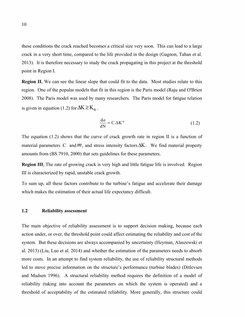
Region II, We can see the linear slope that could fit to the data. Most studies relate to this

region. One of the popular models that fit in this region is the Paris model (Raju and O'Brien

2008). The Paris model was used by many researchers. The Paris model for fatigue relation

is given in equation (1.2) for thK KΔ ≥ .

d

Cd

. KN

ma = Δ (1.2)

The equation (1.2) shows that the curve of crack growth rate in region II is a function of

material parameters C and m , and stress intensity factors KΔ . We find material property

amounts from (BS 7910, 2000) that sets guidelines for these parameters.

Region III, The rate of growing crack is very high and little fatigue life is involved. Region

III is characterized by rapid, unstable crack growth.

To sum up, all these factors contribute to the turbine’s fatigue and accelerate their damage

which makes the estimation of their actual life expectancy difficult.

1.2 Reliability assessment

The main objective of reliability assessment is to support decision making, because each

action under, or over, the threshold point could affect estimating the reliability and cost of the

system. But these decisions are always accompanied by uncertainty (Heyman, Alaszewski et

al. 2013) (Liu, Luo et al. 2014) and whether the estimation of the parameters needs to absorb

more costs. In an attempt to find system reliability, the use of reliability structural methods

led to move precise information on the structure’s performance (turbine blades) (Ditlevsen

and Madsen 1996). A structural reliability method requires the definition of a model of

reliability (taking into account the parameters on which the system is operated) and a

threshold of acceptability of the estimated reliability. More generally, this structure could

11

also include a formulation of the criteria for failure modes that identified failures (Ronold,

Wedel-Heinen et al. 1999), (Moriarty, Holley et al. 2004) (Ditlevsen and Madsen 1996).

What makes the task of analysis difficult is judgment which takes into account parameters

that affect the results (Liu, Luo et al. 2014) (Toft and Sørensen 2011). For this reason, the

Bayesian method is a good technique to account for parameters and consider the related

uncertainties.

CHAPTER 2

UPDATING PARAMETERS WITH BAYESIAN THEORY

2.1 Introduction

The purpose of CHAPTER 2 is to present a Bayesian technique to update the data and

information necessary to reduce uncertainty related to fatigue life reliability. The aviation

industry, particularly in the military field, is at the forefront of scientific developments in the

field of reliability fatigue (Kappas 2002). However, the main difficulties in calculating

reliability is model choice and methodology calculation (Cross, Makeev et al. 2006). The

classic probability methods used with available information may determine reliability. This

method, without updating the information, yields results. Therefore, the uncertainty

associated with the initial parameters is very large, because the information initially available

is limited. But in the new probability methods, one possible solution is to use observations to

update priori estimated values (Wang 2008). This approach is named the Bayesian method.

The Bayesian approach can use the information when it becomes available to combine with

initial hypotheses and prior information to validate the model. The Bayesian theory is a

method for the quantification of uncertainties issues. This method consists of evaluating

Probability Density Function (PDF) for variables and model parameters. (Coppe, Haftka et

al. 2010) used Bayesian inference to reduce the uncertainty of the parameters of a Paris

model in fatigue issues. (Guerin and Hambli 2009) proposed that the Bayesian method is a

possible way to reduce the scatter of fatigue distribution.

In this project, periodic inspections are the main source for gathering information to assist in

the update of model variables for turbine blades. In CHAPTER 2, the Bayesian update

method is used when additional test data are available to decrease the uncertainty of

variables. This leads to the improvement of design optimization and system performance.

The methodology that we used for updating a fatigue model with a Bayesian method is given

in Figure 2.1.

14

Figure 2.1: Methodology that introduces Bayesian updating method to decrease the uncertainty of parameters and variables.

Figure 2.1 shows that the Bayesian theory helps to update prior knowledge in order to obtain

a suitable prediction of fatigue life. We use MCS draw samples from the given distribution.

With the use of Bayesian theory, the uncertainties characterized are reduced. The results of

updated posterior distribution will be used in the reliability analysis found in CHAPTER 3.

We will then compare results in terms of reliability.

2.2 Data uncertainty

Uncertainties come from human errors, model errors, testing methods and measurements.

Although the data are supposed to give us a picture of reality, in truth, because of the

existence of uncertainty, accurately calculating the degree of truth for a given variable cannot

be done (Vorobyev).

According to the difference sources of uncertainties in this project, we first identify a set of

variables and related parameters to be used in this project. Therefore, with the use of the

Bayesian method, which is a type of probabilistic method, the uncertainties associated with

fatigue could decrease in this project.

15

2.3 Hypothesis

It is important to be familiar with hypothesis for more convenience. In general, two types of

material defects are investigated for big structures such as the hydroelectric Francis runner:

surface cracks and near surface cracks (Gagnon, Tahan et al. 2013). To decrease the number

of parameters related to crack geometry, we study the circular cracks located on the surface

in this project. Therefore, we have just one parameter that shows the size of a crack that was

able to grow on a two – dimensional diagram. Figure 2.2 shows the surface, and the near the

surface, crack. We also consider that the crack grows only in one direction where the KΔ is

the maximum amount.

Figure 2.2: Surface crack and near the surface crack (Gagnon, Tahan et al. 2013)

Because of a lack of information about the variables, we only study the stress range and

crack size that are more effective on the fatigue problem and consider other variables that

affect the crack growth rate as constant and deterministic. For example, the stress intensity

factor ( thKΔ ) is first assumed to be constant and well known. This variable is related to

geometry and crack location. The value of ( thKΔ ) and stress intensity correction factor are

taken from the British standard BS7910 (BS 2000). From this standard, the amount of thKΔ

is close to 2 [MPa m1/2].

16

About the fatigue variables (crack size and stress range), we have prior knowledge that

shows these variables follow the normal distribution (Pattabhiraman and Kim 2009). We

want to update the variables when we add the data to our prior knowledge with the Bayesian

method. Therefore if we add more data, the values of updated distributions could be precise

and reduced. As our prior knowledge about the data follow Normal distribution

(Pattabhiraman, 2009), therefore choosing 95% confidence interval for our prior distribution

is more confident about the upper and lower bounds of distribution. This confidence interval

could be a proper measure in our analytical prediction value. Although when we do not have

any idea about the distribution, we could consider the variables following the uniform

distribution (An, Choi et al. 2011). Table 2.1 shows the amount of fatigue problems for the

hydroelectric Francis runner.

Table 2.1: Amount of parameters

Location Upper/Lower band Distribution a [mm] μ =1.5, σ =0.5 [0.2, 2.48] Normal

σΔ [MPa] μ =28, σ =3 [22.12, 33.88] Normal

thKΔ [MPa m1/2] 2

2.4 Bayesian update for fatigue variables

The essential work for using Bayesian statistical analysis is obtaining and estimating the

posterior distribution for variables and model parameters. The posterior is an average

distribution before variables are observed (prior distribution) (Pattabhiraman, 2009). We

then make note of the variables and analyze the information that we observed (likelihood

distribution). In this project we have analytical results (prior) and test variability (likelihood)

that will be used to update posterior distribution to predict fatigue failure and reduce

uncertainty in fatigue issues. This method is good way to decrease uncertainty and provide a

conservative distribution that covers the error of prior distribution and the variability of

likelihood distribution. The relation between the likelihood and prior distribution is shows in

equation (2.1) (Pattabhiraman, 2009).

17

( ) ( ) ( )p test|analitic p (analytic)

p analytic|test p test|analitic p(analytic)p(test)

×= ∝ ×

(2.1)

In this equation ( )p analytic|test is a posterior distribution and ( )p test|analitic is called the

likelihood that introduces the probability of data that achieved from the test given the value

of analytic results. The prior distribution is shown by p (analytic) . The expert opinions

are affected in prior distributions. According to the raw data that is used for Bayesian

updates, therefore the normalizing of data and all distributions is necessary. Therefore, the

dominator of equation (2.1) is brought in to ensure that the posterior PDF integrates to 1. For

updating variables (crack size and stress range) we used equation (2.2) (Pattabhiraman,

2009).

( ) ( )

( )1,test

1,test

0

p X . p (X)p X

p X . p (X) X

ini

ini

i

d+∞=

(2.2)

X in equation (2.2) replaces defect size and stress range. This equation shows that p (X)ini

is the initial distribution of variables. With iterating i times, we could achieve a proper prior

distribution and it is very close to a posterior distribution that could be fit with the data. For

using the Bayesian theory, we follow these steps to obtain precise results:

1) Decide on a prior distribution, with considering the uncertainty in unknown model

parameters before the data observed.

2) Observe the new data and create the likelihood distribution based on the data.

3) Calculate the posterior distribution with a multiplication of prior distribution and

likelihood distribution with simulation.

4) Update the posterior distribution.

18

2.5 Results of updating variables with Bayesian theory

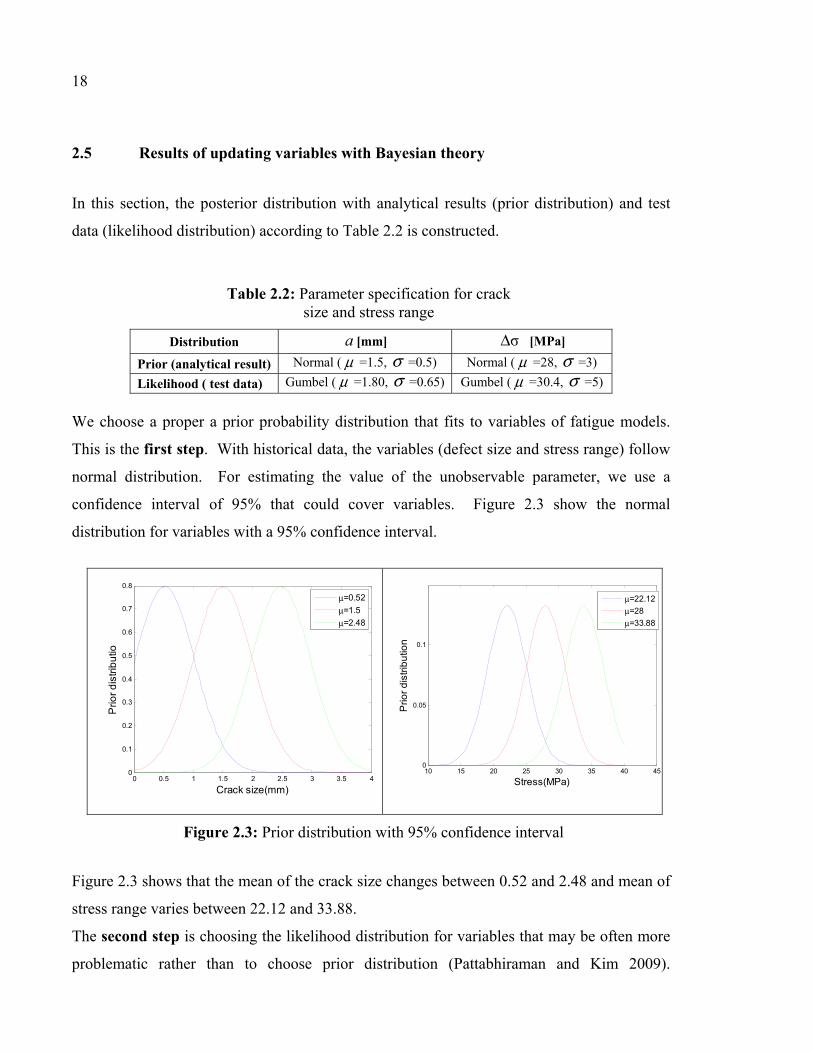
In this section, the posterior distribution with analytical results (prior distribution) and test

data (likelihood distribution) according to Table 2.2 is constructed.

Table 2.2: Parameter specification for crack size and stress range

Distribution a [mm] σΔ [MPa]

Prior (analytical result) Normal ( μ =1.5, σ =0.5) Normal ( μ =28, σ =3)

Likelihood ( test data) Gumbel ( μ =1.80, σ =0.65) Gumbel ( μ =30.4, σ =5)

We choose a proper a prior probability distribution that fits to variables of fatigue models.

This is the first step. With historical data, the variables (defect size and stress range) follow

normal distribution. For estimating the value of the unobservable parameter, we use a

confidence interval of 95% that could cover variables. Figure 2.3 show the normal

distribution for variables with a 95% confidence interval.

Figure 2.3: Prior distribution with 95% confidence interval

Figure 2.3 shows that the mean of the crack size changes between 0.52 and 2.48 and mean of

stress range varies between 22.12 and 33.88.

The second step is choosing the likelihood distribution for variables that may be often more

problematic rather than to choose prior distribution (Pattabhiraman and Kim 2009).

0 0.5 1 1.5 2 2.5 3 3.5 40

0.1

0.2

0.3

0.4

0.5

0.6

0.7

0.8

Crack size(mm)

Prio

r dis

tribu

tio

μ=0.52μ=1.5μ=2.48

10 15 20 25 30 35 40 450

0.05

0.1

Stress(MPa)

Prio

r dis

tribu

tion

μ=22.12μ=28μ=33.88

19

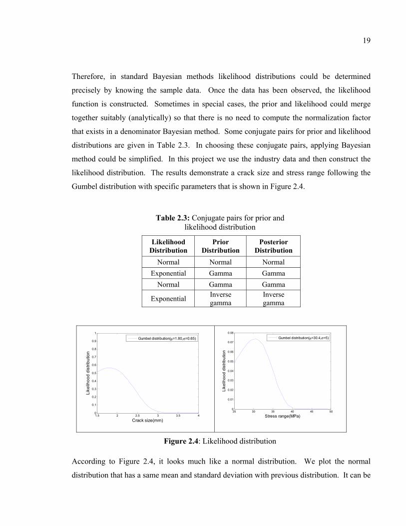
Therefore, in standard Bayesian methods likelihood distributions could be determined

precisely by knowing the sample data. Once the data has been observed, the likelihood

function is constructed. Sometimes in special cases, the prior and likelihood could merge

together suitably (analytically) so that there is no need to compute the normalization factor

that exists in a denominator Bayesian method. Some conjugate pairs for prior and likelihood

distributions are given in Table 2.3. In choosing these conjugate pairs, applying Bayesian

method could be simplified. In this project we use the industry data and then construct the

likelihood distribution. The results demonstrate a crack size and stress range following the

Gumbel distribution with specific parameters that is shown in Figure 2.4.

Table 2.3: Conjugate pairs for prior and likelihood distribution

Likelihood Distribution

Prior Distribution

Posterior Distribution

Normal Normal Normal

Exponential Gamma Gamma

Normal Gamma Gamma

Exponential Inverse gamma

Inverse gamma

Figure 2.4: Likelihood distribution

According to Figure 2.4, it looks much like a normal distribution. We plot the normal

distribution that has a same mean and standard deviation with previous distribution. It can be

1.5 2 2.5 3 3.5 40

0.1

0.2

0.3

0.4

0.5

0.6

0.7

0.8

0.9

1

Crack size(mm)

Like

lihoo

d di

strib

utio

n

Gumbel distribution(μ=1.80,σ=0.65)

25 30 35 40 45 500

0.01

0.02

0.03

0.04

0.05

0.06

0.07

0.08

Stress range(MPa)

Like

lihoo

d di

strib

utio

n

Gumbel distribution(μ=30.4,σ=5)

20

seen in Figure 2.5. We do this work when we want to obtain the suitable distribution

between Normal and Gumbel to cover most values. Also, Figure 2.5 shows the product

distribution that is an average of them.

Figure 2.5: Likelihood distribution and product distribution

Figure 2.5 shows the product distribution that it used for updating variables. Figure 2.6 also

shows the prior and likelihood distribution with each other.

0.5 1 1.5 2 2.5 3 3.5 40

0.1

0.2

0.3

0.4

0.5

0.6

0.7

0.8

0.9

1

Crack size(mm)

Pro

babi

lity

dist

ribut

ion

Gumbel distributionNormal distributionProduct distribution

10 15 20 25 30 35 40 45 500

0.01

0.02

0.03

0.04

0.05

0.06

0.07

0.08

0.09

0.1

Stress range(MPa)

Pro

babi

lity

dist

ribut

ion

Gumbel distributionNormal distributionProduct distribution

21

Figure 2.6: Prior and likelihood distribution

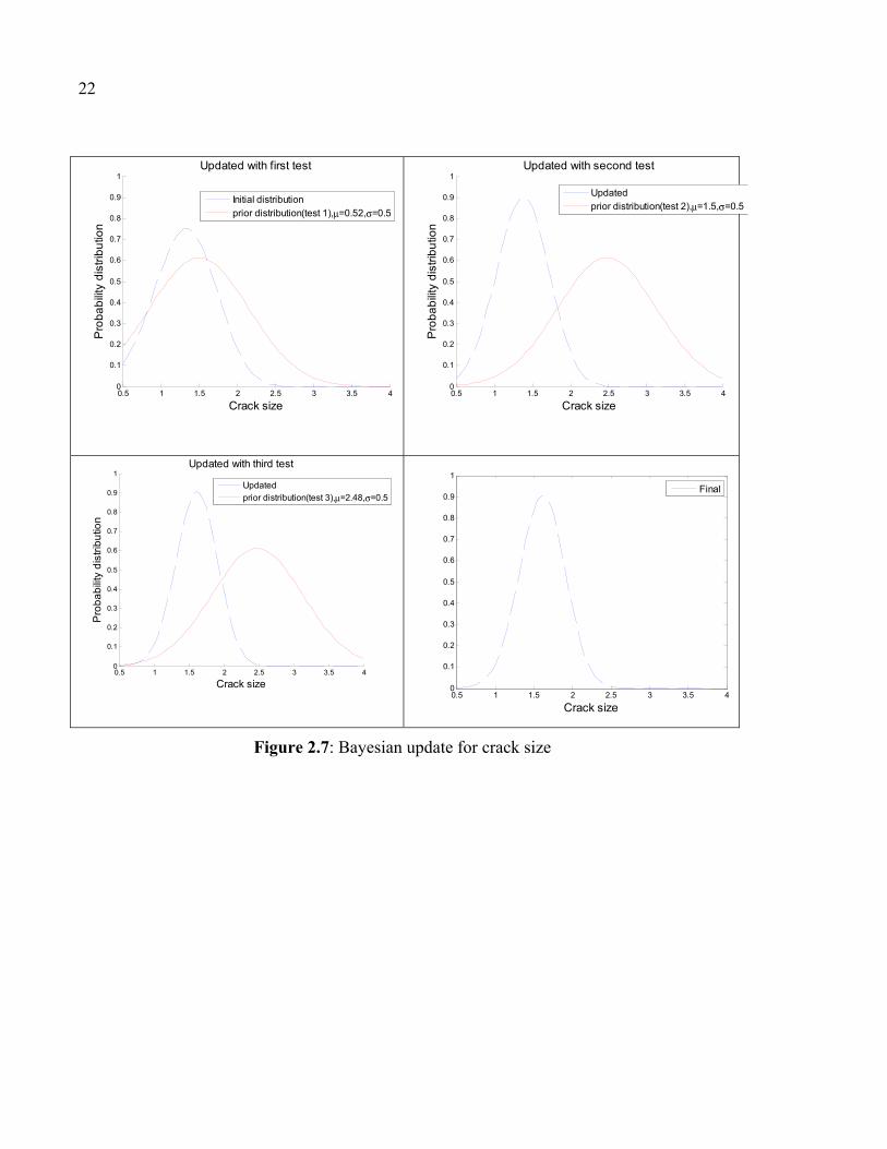
Having the prior and likelihood distribution, we could estimate the posterior distribution. We

also update posterior distribution with a confidence interval of 95% to not miss the data.

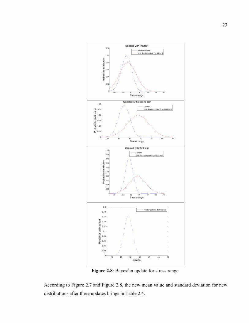
Figure 2.7 and Figure 2.8 show variables updated with the Bayesian method.

0.5 1 1.5 2 2.5 3 3.5 40

0.1

0.2

0.3

0.4

0.5

0.6

0.7

0.8

0.9

1

Crack size

Pro

babi

lity

dist

ribut

ion

Initial distribution

product distributionprior distribution(test 1),μ=0.52,σ=0.5

5 10 15 20 25 30 35 40 45 500

0.01

0.02

0.03

0.04

0.05

0.06

0.07

0.08

0.09

0.1

Stress range

Pro

babi

lity

dist

ribut

ion

Initial distribution

product distributionprior distribution(test 1),μ=22.12,σ=3

22

Figure 2.7: Bayesian update for crack size

0.5 1 1.5 2 2.5 3 3.5 40

0.1

0.2

0.3

0.4

0.5

0.6

0.7

0.8

0.9

1

Crack size

Pro

babi

lity

dist

ribut

ion

Updated with first test

Initial distributionprior distribution(test 1),μ=0.52,σ=0.5

0.5 1 1.5 2 2.5 3 3.5 40

0.1

0.2

0.3

0.4

0.5

0.6

0.7

0.8

0.9

1

Crack size

Pro

babi

lity

dist

ribut

ion

Updated with second test

Updatedprior distribution(test 2),μ=1.5,σ=0.5

0.5 1 1.5 2 2.5 3 3.5 40

0.1

0.2

0.3

0.4

0.5

0.6

0.7

0.8

0.9

1

Crack size

Pro

babi

lity

dist

ribut

ion

Updated with third test

Updatedprior distribution(test 3),μ=2.48,σ=0.5

0.5 1 1.5 2 2.5 3 3.5 40

0.1

0.2

0.3

0.4

0.5

0.6

0.7

0.8

0.9

1

Crack size

Final

23

Figure 2.8: Bayesian update for stress range

According to Figure 2.7 and Figure 2.8, the new mean value and standard deviation for new

distributions after three updates brings in Table 2.4.

20 25 30 35 40 45 500

0.02

0.04

0.06

0.08

0.1

0.12

Stress range

Pro

babi

lity

dist

ribut

ion

Updated with first test

Initial distributionprior distribution(test 1),μ=28,σ=3

20 25 30 35 40 45 500

0.02

0.04

0.06

0.08

0.1

0.12

Stress range

Pro

babi

lity

dist

ribut

ion

Updated with second test

Updatedprior distribution(test 2),μ=33.88,σ=3

20 25 30 35 40 45 500

0.02

0.04

0.06

0.08

0.1

0.12

0.14

0.16

0.18

0.2

Stress range

Pro

babi

lity

dist

ribut

ion

Updated with third test

Updatedprior distribution(test 3),μ=33.99,σ=5

20 25 30 35 40 45 500

0.02

0.04

0.06

0.08

0.1

0.12

0.14

0.16

0.18

0.2

stress

Pos

terio

r dis

tribu

tion

Final (Posterior distribution)

24

Table 2.4: Mean value and standard deviation for updated distribution

Distribution a [mm] σΔ [MPa]

Prior (analytical result) Normal ( μ =1.5, σ =0.5) Normal ( μ =28, σ =3)

Likelihood ( test data) Gumbel ( μ =1.80, σ =0.65) Gumbel ( μ =30.4, σ =5)

Posterior μ =1.6, σ =0.5 μ =29.1, σ =0.75

Note that the amount of standard deviations for updated posterior distributions is decreased

by 33% for crack size and 83% for stress range. Therefore updating the likelihood

distribution with three test data sets reduces the uncertainty of fatigue variables.

2.6 Results of updating parameters with Bayesian theory

In the previous section, the variables of fatigue problems were updated with the Bayesian

method. However, in predicting fatigue life, updating variable parameters is also

recommended (Pattabhiraman, 2009). In this section, we want to update the parameters

mean value and standard deviation ( μ ,σ ) of variables using the Bayesian method to

decrease the additional uncertainties that exist in fatigue issues. As mentioned earlier,

choosing a proper probability distribution as a prior for parameters is the first step in the

Bayesian method. From the results shown in Table 2.4, we are interested in choosing a

probability distribution function for the data with this amount of posterior distribution.

As we know, the parameter amounts affect to the skew and median of distribution, therefore

it is important to obtain precise amount parameters because to construct limit states, we need

to use these parameters amounts. Therefore, with accurate limit states we can estimate a

proper reliability index. So we should model these parameters and study them to decrease

the uncertainties that exist in parameters by using new information.

For this study, we consider that μ follows noninformative (uniform distribution) with

domain [ ],b c (equation (2.3)). This kind of distribution is very common to use when you do

not have an idea of the parameters (An, Choi et al. 2011).

25

( )

0

1

0

b

p b cb c

c

μ

μμ

μ

<= ≤ ≤ −

>

(2.3)

To decrease the uncertainty ofσ , we notice that it follows the normal distribution. The

equation (2.3) shows the normal probability distribution. The second step is constructing the

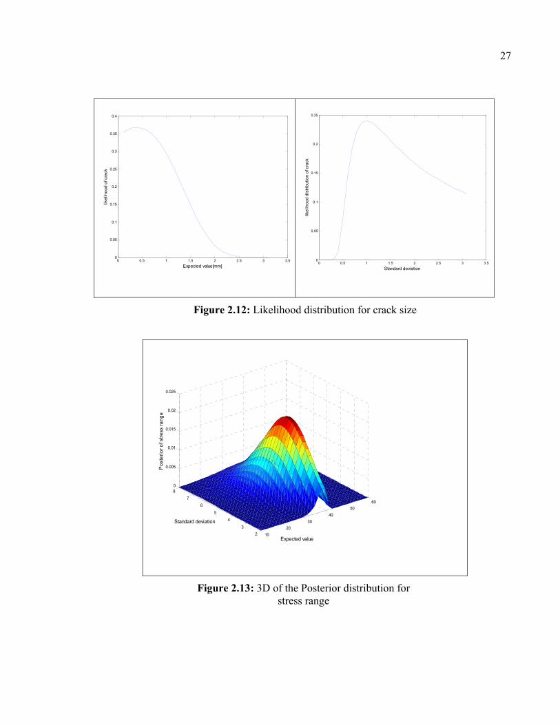
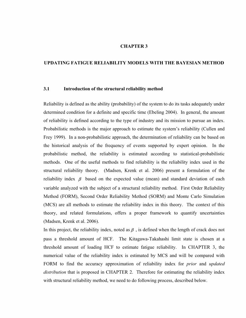
likelihood distribution from the data that was given in Table 2.4. Figure 2.9 to Figure 2.12

are a prior and likelihood probability distribution of a variation of parameters for stress range

and crack size. The third step is the derivation of posterior distribution using Bayesian

theory. Figure 2.14 and Figure 2.14 show the 3D of the posterior distribution for stress

ranges and crack size. The result of posterior distribution is shown in Table 2.5.

Table 2.5: Amount of parameters related to σΔ and a with prior and likelihood distribution

Prior Likelihood Posterior

σΔ μ is uniform with domain [10 - 60].

( )~ 1,1.5Nσ Gumbel ( μ =29.1,σ =0.75)

μ =28.41

σ =0.495

a μ is uniform with domain [0.1 , 3.1].

( )~ 0.55,0.2Nσ Gumbel( μ =1.6,σ =0.5)

μ =1.577

σ =0.435

Figure 2.9 : Prior probability distribution for stress range

10 15 20 25 30 35 40 45 50 55 60-1

-0.5

0

0.5

1

1.5

Expected value

Prio

r of s

tress

par

amet

er

2 3 4 5 6 7 80

0.05

0.1

0.15

0.2

0.25

0.3

0.35

Standard deviation

Prio

r of s

tress

par

amet

er

26

Figure 2.10: Likelihood probability distribution for stress range

Figure 2.11: Prior probability distribution for crack size

10 15 20 25 30 35 40 450

0.01

0.02

0.03

0.04

0.05

0.06

0.07

0.08

0.09

0.1

Expected value

likel

ihoo

d of

stre

ss p

aram

eter

2 3 4 5 60.04

0.05

0.06

0.07

0.08

0.09

0.1

0.11

0.12

Standard deviation

likel

ihoo

d di

strib

utio

nof s

tress

par

amet

er

0 0.5 1 1.5 2 2.5 3 3.5-1

-0.5

0

0.5

1

1.5

Expected value[mm]

Prio

r of c

rack

0 0.5 1 1.5 2 2.5 3 3.50

0.2

0.4

0.6

0.8

1

1.2

1.4

1.6

1.8

2

Standard deviation

Prio

r of c

rack

27

Figure 2.12: Likelihood distribution for crack size

Figure 2.13: 3D of the Posterior distribution for stress range

0 0.5 1 1.5 2 2.5 3 3.50

0.05

0.1

0.15

0.2

0.25

0.3

0.35

0.4

Expected value[mm]

likel

ihoo

d of

cra

ck

0 0.5 1 1.5 2 2.5 3 3.50

0.05

0.1

0.15

0.2

0.25

Standard deviation

likel

ihoo

d di

strib

utio

n of

cra

ck

1020

3040

5060

23

45

67

80

0.005

0.01

0.015

0.02

0.025

Expected value

Standard deviation

Pos

terio

r of s

tress

rang

e

28

Figure 2.14: 3D of the Posterior distribution for crack size

2.7 Conclusion:

We used an update of the Bayesian method to estimate the amount of variables in section 2.5.

The results show that the Bayesian method is a good way to reduce uncertainty in fatigue

issues. We see that the standard deviation for crack size and stress range is reduced by more

than 30% and 80%. If more data are gathered, the values of posterior distribution could be

updated; therefore the credible interval could be decreased. For this reason, in section 2.6,

we update the parameters of variables. We thus achieve a conservative estimate of the

variables. So with Bayesian theory we did a proper distribution with minimum uncertainties

in parameters. In CHAPTER 3, we use the results of CHAPTER 2 to estimate the fatigue

reliability index.

00.5

11.5

22.5

33.5

0

1

2

3

40

0.01

0.02

0.03

0.04

0.05

Expected value of crackStandard deviation of crack

Pos

terio

r of c

rack

CHAPTER 3

UPDATING FATIGUE RELIABILITY MODELS WITH THE BAYESIAN METHOD

3.1 Introduction of the structural reliability method

Reliability is defined as the ability (probability) of the system to do its tasks adequately under

determined condition for a definite and specific time (Ebeling 2004). In general, the amount

of reliability is defined according to the type of industry and its mission to pursue an index.

Probabilistic methods is the major approach to estimate the system’s reliability (Cullen and

Frey 1999). In a non-probabilistic approach, the determination of reliability can be based on

the historical analysis of the frequency of events supported by expert opinion. In the

probabilistic method, the reliability is estimated according to statistical-probabilistic

methods. One of the useful methods to find reliability is the reliability index used in the

structural reliability theory. (Madsen, Krenk et al. 2006) present a formulation of the

reliability index β based on the expected value (mean) and standard deviation of each

variable analyzed with the subject of a structural reliability method. First Order Reliability

Method (FORM), Second Order Reliability Method (SORM) and Monte Carlo Simulation

(MCS) are all methods to estimate the reliability index in this theory. The context of this

theory, and related formulations, offers a proper framework to quantify uncertainties

(Madsen, Krenk et al. 2006).

In this project, the reliability index, noted as β , is defined when the length of crack does not

pass a threshold amount of HCF. The Kitagawa-Takahashi limit state is chosen at a

threshold amount of loading HCF to estimate fatigue reliability. In CHAPTER 3, the

numerical value of the reliability index is estimated by MCS and will be compared with

FORM to find the accuracy approximation of reliability index for prior and updated

distribution that is proposed in CHAPTER 2. Therefore for estimating the reliability index

with structural reliability method, we need to do following process, described below.

30

3.2 Step 1: Identify the significant failure modes of hydroelectric turbine blades

As mentioned earlier, operating mode, maintenance strategy, quality of repairs, initial size of

the crack by the manufacturer, location and shape of crack, along with stress loading are all

parameters that influence the reliability index of fatigue (Raju and O'Brien 2008), (Gagnon,

Tahan et al. 2013). CHAPTER 2 identifies the main variables in our model (e.g. crack size

and stress range) which lead to the cracking of the hydroelectric turbine’s blades that cause

the degradation of the system’s reliability. Therefore the fatigue reliability in hydroelectric

turbines depends on the probabilistic model of a crack length that does not increase after

passing a number of cycles under specific loading.

3.3 Step 2: Define probability of failure for turbine blades

Roughly, we could separate variables which affect the system in two groups

(VĂCĂREANU, 2007 ). One of them shows the resistance (strength) of system R versus of

loading (stress) S that disturbs the system. Failure will happen when R is less than load S.

Each of these variables follows a specific probability density function ( ()Sf and ()Rf ), it is

important to study the joint distribution of each to find the probability of failure. In this

specific case, R and S are said in the same units (e.g. MPa). Figure 3.1 shows an example for

distributions of resistance and load variables when their joint distribution may lead to the

failure of the system.

Figure 3.1: Basic failure problem (VĂCĂREANU, ALDEA et al. 2007)

31

The gray area in Figure 3.1 shows that some probability for loads in this area surpass

resistance behavior. Therefore the probability of failure FP r in this area needs to be

estimated. With a structural reliability method, the probability failure FP r could be obtained

easily, with new variables. This relation can be stated in equation (3.1) (Melchers 1999).

F

0Pr( 0) (P ) ( )r z

z

Z μ βσ−≤ = Φ= Φ = − (3.1)

In this equation Φ is the standard normal cumulative distribution function, and β is defined

as the reliability index. All of the variables exist in a normal distribution form. As we see in

equation (3.1) when the standard deviation zσ is increased, the probability of failure will

increase. But in most cases, this simple equation is not appropriate to solve the problem.

More general formulation is required. With the theory of the structural reliability method

this problem is solved whether it defines the equation that is a safe boundary and in unsafe

mode. This equation is named a limit state and shows with g ( )X . The X is the vector of

all relevant basic variables. In general, the limit state equation is derived from the physics of

the problem. A failure in the structural reliability method is functional of the limit state when

the limit state is less than zero ( g( ) 0≤X ). The probability of failure is evaluated as equation

(3.2) and could be written as equation (3.3).

{ }F Pr g )Pr ( 0= ≤X (3.2)

F g( ) 0(r )P f d

≤= X

X x (3.3)

When the limit state is less than zero it shows the unsafe state. Various methods for solutions

of the integral in equation (3.3) have been proposed. Some limit states are linear and an

analytical solution is easy to obtain. If limit state functions are nonlinear, we can obtain an

approximate solution by linearizing the function using a Taylor series development. FORM,

SORM and MCS are frequently used to calculate a reliability index when we have a

nonlinear limit state. In all these methods the equation of limit state is equal to zero (

g( ) 0=X ) and the reliability index ( β ) is definite as the shortest distance from the origin of

standards and normalized variables to the limit state in the same iso-probabilistic space. This

definition, which is introduced by (Hasofer and Lind 1974) is seen in Figure 3.2.

32

Figure 3.2: Reliability index on nonlinear limit state (Hasofer and Lind 1974)

Figure 3.2 shows the desire point to have a reliability index on the nonlinear limit state. It

could be estimated with an iteration relation.

3.4 Step 3: Construct Kitagawa-Takahashi limit state for fatigue reliability

It must be considered in fatigue failure; the Kitagawa-Takahashi limit state is more used

(Kruzic and Ritchie 2006). For constructing the Kitagawa-Takahashi limit, data from S-N

approach and LEFM approach are used. (Gagnon, Tahan et al. 2013) used the Kitagawa-

Takahashi limit state for the HCF onset to estimate the fatigue reliability for turbine blades.

As mentioned in CHAPTER 1, no propagation occurs in Region I below a threshold stress

intensity factor. Equation (3.4) is used to determine the stress range at HCF with the LEFM

method. This equation shows the relation between the HCF stress range at threshold point

thσΔ and stress intensity factor at threshold point thKΔ .

33

( )th

th

Kσ

πa aγΔΔ = (3.4)

With equation (3.4) and data from the S-N curve, the Kitagawa-Takahashi limit state could

be evaluated in 2D space by equation (3.5).

( )( )thK

a, σ σπa a

gγ

ΔΔ = Δ − (3.5)

In this equation, g () is the limit state and function of variables (defect size a [mm] and

stress range σΔ [MPa]). Later (El Haddad, Topper et al. 1979) proposed some corrections

to the limit state. Figure 3.3 shows a schematic of the Kitagawa –Takahashi limit state with

an El Haddad correction.

Figure 3.3: Schematic of Kitagawa -Takahashi limit state with El Haddad correction (Gagnon,

Tahan et al. 2013)

Figure 3.3 shows the Kitagawa-Takahashi limit state with Log-Log scales. One line is the

fatigue limit and represents the limit of the material’s resistance and is determined with an S-

N approach. In this study, it corresponds to 107 cycles when the crack is in the surface and

has a circle shape. The second line is represented by the stress range at a threshold point that

is obtained by the LEFM approach (equation (3.4)).

34

3.4.1 Estimated reliability index for the standard normal variables

The standard normal distribution is used to estimate the reliability index β . It is easy to

analyze and at this form the variable does not have dimensional consistency. The relation

(3.6) shows a standard normal form (Z) for variables. As we mentioned in this project the

stress range and crack defect are the main variables.

X

X

X

XZσ

i i

i

i

μ−= (3.6)

Equation (3.6) reduced all of the normal variables to the standard form. According to the real

problem, the variables follow non-normal distribution; we need to transfer the variables from

the non-normal space to a standard normal space (iso-probabilistic space). One of the

transformation techniques that could be used is a Rosenblatt transformation. In this project

we use a Rosenblatt transformation to reduced variables in a standard normal space.

3.4.2 Rosenblatt transformation

When the variables are non-normal, the Rosenblatt transformation is applicable and shows up

in equation (3.7).

( )1X( X )Z F−Φ= (3.7)

Where ( )X XF is the cumulative distribution (CDF) of X , Φ is the standard normal

cumulative distribution. For generating the new expected value and the standard deviation

that relates to equation (3.7), we need to define the relation that is described in (3.8) to (3.9).

X

X( ) (X )

i

i ii

i

Fμσ−Φ = (3.8)

X

1 X( ) (X )

i

i ii

i i

fμϕσ σ

− = (3.9)

Where X (X )i if is the probability density function (PDF) for ,μ σ . The new ,μ σ could be

obtained by (3.10) to (3.11) are:

35

1X

X

( ( (X ))

(X )i

i

ii

i

Ff

ϕσ

−Φ= (3.10)

1XX ( (X ))

ii i i iFμ σ −= − Φ (3.11)

3.4.3 Estimating reliability index with FORM

As mentioned, the reliability index represents the shortest distance from the origin to the

point in a limit state when all of the variables are in the standard normal form. When the

limit state is nonlinear, we can obtain an approximate answer by linearizing the function

using a Taylor series. Equation (3.12) is used to linearize the limit state.

( ) ( )* * * *1 2 1 1

1

, , , , ,.., ( )n

n n i i evaluated at design pointi i

gg X X X g x x x X xX=

∂… ≈ + −∂ (3.12)

The design point *ix is a point on the limit state when the limit state is equal to zero. Since

this design point is generally not known, an iterative technique must be used to solve the

equation. Equations (3.13a) to (3.13c) show the iteration that is needed to find the reliability

index. Calculating this equation needs additional time in order to find the location of a

design point. For calculating the design point, we need reduced variables. Therefore all of

the variables need to be transferred to a standard normal variable.

int

2

1

int

Z

)Z

(

evaluatedatdesignpo

i

n

evaluatedatKdes

i

Kign

po

g

g

α

=

∂∂

=

∂∂

(3.13c)

( )* * *1 2Z , Z ,..., Z 0ng = ;

*Zi iβα= (3.13a)

X

Z X Zi

i

ii

g g∂ ∂ ∂=∂ ∂ ∂

(3.13b)

36

The probability failure is estimated directly from the reliability index and is given by

equation (3.14).

F

0Pr ( <0)= ( ) (- )X

X

X μ βσ−Φ = Φ (3.14)

3.5 Estimate reliability index for prior distribution

As mentioned before, in order to estimate the reliability index, the first step is constructing

the limit state with variables that affect the failure. With the use of information in Table 3.1,

the Kitagawa-Takahashi limit state constructed.

Table 3.1: Detailed results for a [mm] (Normal ( μ =1.5, σ =0.5)) and σΔ [MPa] (Normal ( μ

=28 σ =3))

Description for Prior distribution Values

Physical space design point (mm, MPa) (1.5, 28)

Standard space design point (1.79, 1.88)

MCS reliability index (105 simulations) 2.60

FORM reliability index 1.88

MCS probability failure 0.004

FORM probability failure 0.029

After constructing the limit state, we could estimate the reliability index when the variables

are reduced to the normal standard space. The prior distribution in this study follows normal;

therefore we do not need to use transformation technique. After updating the results

(updated to posterior distribution) we will use a Rosenblatt transformation to transfer

variables to a 2D standard normal space. Figure 3.4 shows the limit state and β when all of

the variables are in standard form. The value of reliability index is calculated by MCS

method and FORM.

37

.

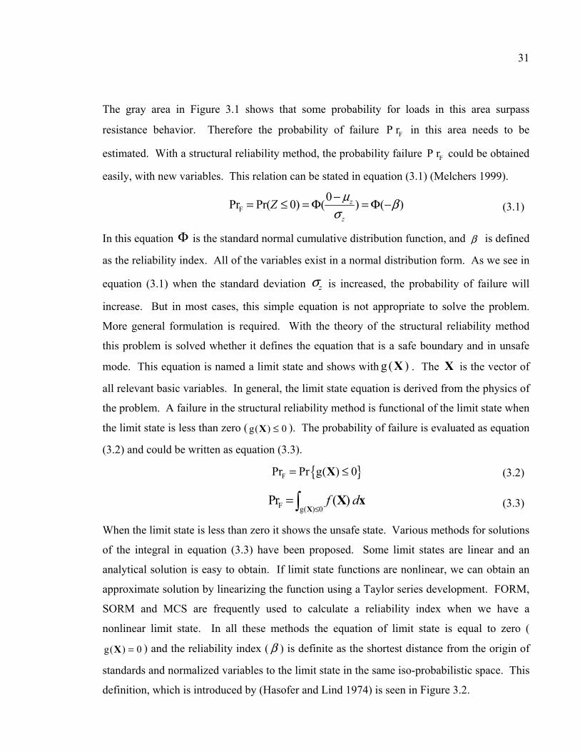
Figure 3.4: Reliability index amount

Figure 3.4 shows the result of reliability index for the crack that obtained by MCS after 105

simulations. We generate 105 data because the amount of reliability is between 2 and 4. In

general for large amount of reliability index we need to simulate more than 106 data. This

amount has abilities to cover distribution that need to investigate. According to in this

project, reliability index is close to 3, selecting the number of 105 simulations is reasonable.

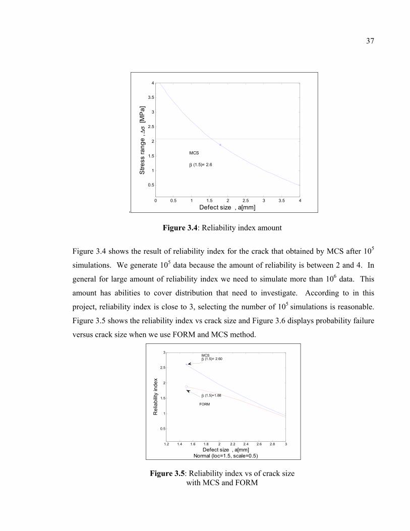
Figure 3.5 shows the reliability index vs crack size and Figure 3.6 displays probability failure

versus crack size when we use FORM and MCS method.

Figure 3.5: Reliability index vs of crack size with MCS and FORM

0 0.5 1 1.5 2 2.5 3 3.5 4

0.5

1

1.5

2

2.5

3

3.5

4

Defect size , a[mm]

Stre

ss ra

nge

, Δσ

[MP

a]

β (1.5)= 2.6

MCS

1.2 1.4 1.6 1.8 2 2.2 2.4 2.6 2.8 3

0.5

1

1.5

2

2.5

3

Defect size , a[mm]Normal (loc=1.5, scale=0.5)

Rel

iabi

lity

inde

x

β (1.5)= 2.60

β (1.5)=1.88

MCS

FORM

38

Figure 3.6: Probability of failure vs crack size with MCS and FORM

Figure 3.5 and Figure 3.6 show the large difference between MCS and FORM. However, in

both cases, the results follow the same trend, but the amounts are different from each other.

One of the reasons is because of existing of large standard deviation of variables specially

related to stress range. As we see the equation in (3.13), the impact of the standard deviation

in the FORM method is very high. But after updating variables and decreasing uncertainties

we will see the curves of FORM and MCS converge to each other. Although we need to

consider that the results for FORM are obtained with only 16 iterations as compared to MCS

those 105 simulations which draws from the distribution.

3.6 Estimate reliability index for posterior distribution

After estimating the reliability index for prior distribution, we need to update the results to

use posterior distribution to achieve precise fatigue reliability. As mentioned in CHAPTER

2, the product of prior and likelihood is posterior distribution. The amount of parameters for

posterior distribution are taken from Table 2.4 to construct the limit state. Afterwards, the

use of Rosenblatt transformation and the variables transfer to the 2D standard normal space

to estimate the reliability index. Figure 3.7 shows the reliability index point that is obtained

1.5 2 2.5 30

0.05

0.1

0.15

0.2

0.25

0.3

0.35

0.4

Defect size , a[mm]Normal (loc=a, scale=0.5)

Pro

babi

lity

failu

re

MC

FORM

MC

FORM

MC

FORM

39

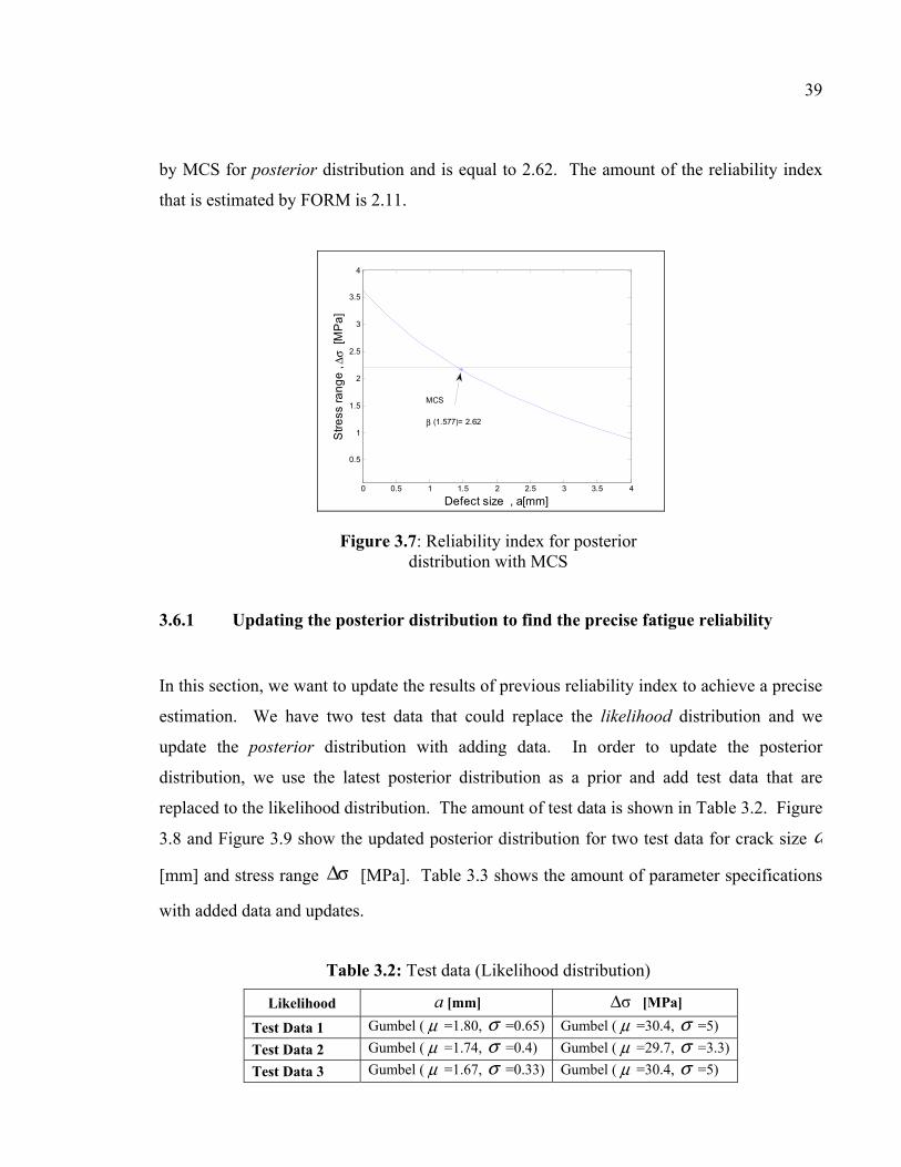
by MCS for posterior distribution and is equal to 2.62. The amount of the reliability index

that is estimated by FORM is 2.11.

Figure 3.7: Reliability index for posterior distribution with MCS

3.6.1 Updating the posterior distribution to find the precise fatigue reliability

In this section, we want to update the results of previous reliability index to achieve a precise

estimation. We have two test data that could replace the likelihood distribution and we

update the posterior distribution with adding data. In order to update the posterior

distribution, we use the latest posterior distribution as a prior and add test data that are

replaced to the likelihood distribution. The amount of test data is shown in Table 3.2. Figure

3.8 and Figure 3.9 show the updated posterior distribution for two test data for crack size a

[mm] and stress range σΔ [MPa]. Table 3.3 shows the amount of parameter specifications

with added data and updates.

Table 3.2: Test data (Likelihood distribution)

Likelihood a [mm] σΔ [MPa]

Test Data 1 Gumbel ( μ =1.80, σ =0.65) Gumbel ( μ =30.4, σ =5)

Test Data 2 Gumbel ( μ =1.74, σ =0.4) Gumbel ( μ =29.7, σ =3.3)

Test Data 3 Gumbel ( μ =1.67, σ =0.33) Gumbel ( μ =30.4, σ =5)

0 0.5 1 1.5 2 2.5 3 3.5 4

0.5

1

1.5

2

2.5

3

3.5

4

Defect size , a[mm]

Stre

ss ra

nge

, Δσ

[MP

a]

β (1.577)= 2.62

MCS

40

Figure 3.8: Two updated posterior distribution for crack size

0.5 1 1.5 2 2.5 30

0.1

0.2

0.3

0.4

0.5

0.6

0.7

0.8

0.9

1

Crack size

Pro

babi

lity

dist

ribut

ion

Posterior distribution

0.5 1 1.5 2 2.5 30

0.1

0.2

0.3

0.4

0.5

0.6

0.7

0.8

0.9

1

Crack size

1th updated-Posterior distribution

0.5 1 1.5 2 2.5 30

0.1

0.2

0.3

0.4

0.5

0.6

0.7

0.8

0.9

1

Crack size

2th updated-Posterior distribution

20 25 30 350

0.02

0.04

0.06

0.08

0.1

0.12

0.14

0.16

0.18

0.2

stress

Posterior distribution

27 27.5 28 28.5 29 29.5 30 30.5 310

0.1

0.2

0.3

0.4

0.5

0.6

0.7

0.8

0.9

1

stress

1th-Updated posterior distribution

41

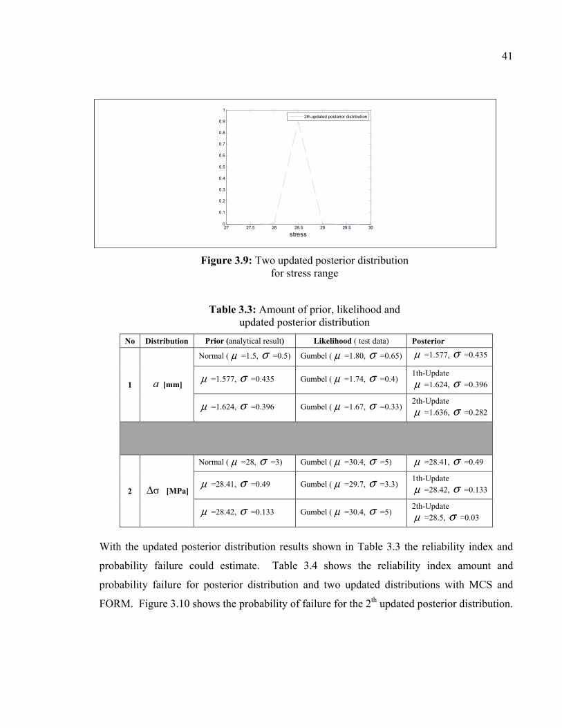
Figure 3.9: Two updated posterior distribution for stress range

Table 3.3: Amount of prior, likelihood and updated posterior distribution

No Distribution Prior (analytical result) Likelihood ( test data) Posterior

1 a [mm]

Normal ( μ =1.5, σ =0.5) Gumbel ( μ =1.80, σ =0.65) μ =1.577, σ =0.435

μ =1.577, σ =0.435 Gumbel ( μ =1.74, σ =0.4) 1th-Update

μ =1.624, σ =0.396

μ =1.624, σ =0.396 Gumbel ( μ =1.67, σ =0.33) 2th-Update

μ =1.636, σ =0.282

2 σΔ [MPa]

Normal ( μ =28, σ =3) Gumbel ( μ =30.4, σ =5) μ =28.41, σ =0.49

μ =28.41, σ =0.49 Gumbel ( μ =29.7, σ =3.3) 1th-Update

μ =28.42, σ =0.133

μ =28.42, σ =0.133 Gumbel ( μ =30.4, σ =5) 2th-Update

μ =28.5, σ =0.03

With the updated posterior distribution results shown in Table 3.3 the reliability index and

probability failure could estimate. Table 3.4 shows the reliability index amount and

probability failure for posterior distribution and two updated distributions with MCS and

FORM. Figure 3.10 shows the probability of failure for the 2th updated posterior distribution.

27 27.5 28 28.5 29 29.5 300

0.1

0.2

0.3

0.4

0.5

0.6

0.7

0.8

0.9

1

stress

2th-updated posterior distribution

42

Table 3.4: Reliability index and probability failure for updated distribution

No Distribution β

MCS

β

FORM

FPr

MCS

FPr

FORM

1 Prior 2.60 1.88 0.004 0.029

2 Posterior 2.62 2.11 0.004 0.017

3 1th-Update 2.06 2.08 0.019 0.018

4 2th-Update 1.75 1.99 0.039 0.023

Figure 3.10: Evolution of the probability of failure vs crack size

Figure 3.10 shows that probability failure increases when the crack size grows. Also, we see

that the difference of FORM and MCS is near to zero after the 2th updater of posterior

distribution which causes a decrease in the uncertainty of parameters. We can see and

compare the probability of failure for the prior and posterior distribution with FORM and

MCS methods as shown in Figure 3.11 and Figure 3.12.

43

Figure 3.11: Probability of failure for prior and 2th updated posterior distribution with FORM

method

Figure 3.12: Probability of failure for prior and 2th updated posterior distribution with MCS

method

1.8 2 2.2 2.4 2.6 2.8 30

0.05

0.1

0.15

0.2

0.25

0.3

0.35

0.4

Defect size , a[mm]

Pro

babi

lity

failu

re

2th updated Posterior Prior distribution

1.8 2 2.2 2.4 2.6 2.8 30

0.05

0.1

0.15

0.2

0.25

0.3

0.35

0.4

Defect size , a[mm]

Pro

babi

lity

failu

re

2th Updated Posterior distribution/FROMPrior distribution

44

As we see in Figure 3.11 and Figure 3.12, the amount of probability failure for posterior

distribution is less than the prior distribution. Therefore, the failure occurs sooner than we

expected. .

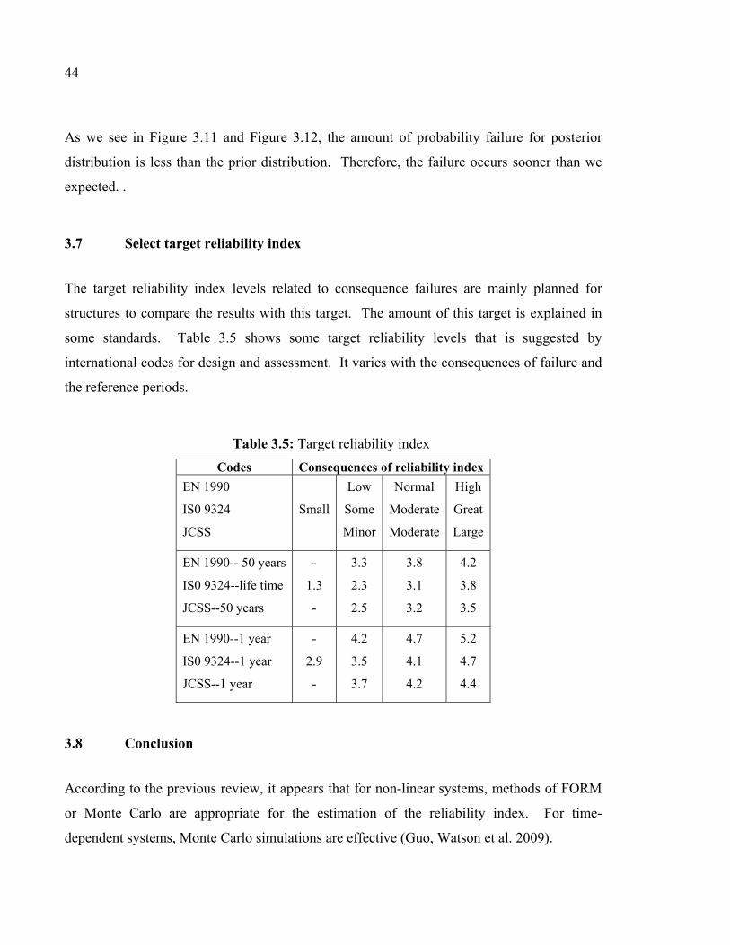
3.7 Select target reliability index

The target reliability index levels related to consequence failures are mainly planned for

structures to compare the results with this target. The amount of this target is explained in

some standards. Table 3.5 shows some target reliability levels that is suggested by

international codes for design and assessment. It varies with the consequences of failure and

the reference periods.

Table 3.5: Target reliability index

Codes Consequences of reliability index

EN 1990

IS0 9324

JCSS

Small

Low

Some

Minor

Normal

Moderate

Moderate

High

Great

Large

EN 1990-- 50 years

IS0 9324--life time

JCSS--50 years

-

1.3

-

3.3

2.3

2.5

3.8

3.1

3.2

4.2

3.8

3.5

EN 1990--1 year

IS0 9324--1 year

JCSS--1 year

-

2.9

-

4.2

3.5

3.7

4.7

4.1

4.2

5.2

4.7

4.4

3.8 Conclusion

According to the previous review, it appears that for non-linear systems, methods of FORM

or Monte Carlo are appropriate for the estimation of the reliability index. For time-

dependent systems, Monte Carlo simulations are effective (Guo, Watson et al. 2009).

45

The value of the reliability index must be accompanied by a probability of failure based on

the updated prediction of crack growth rates. For calculating the reliability index, a

Rosenblatt transformation technique is used to obtain a representation in iso-probabilistic

space. After constructing the limit state with variables in standard form, we first estimate the

reliability index for prior distribution with FORM and MCS methods. The accuracy of the

FORM is compared with the MCS that was shown in Figure 3.10. We understand that when

the uncertainties are large, the differences of MCS and FORM are considerable. After

updating the distribution with Bayesian methodology, results show that the standard

deviation of a stress range is changed (better estimation) and the differences of reliability

index with FORM and MCS are smaller than before. As shown, the reliability index is very

dependent on the type of distribution of variables and the amount of parameters. Therefore,

determining the precise distribution affects estimating the reliability index. With an updated

reliability index and a probability of failure, we could better-placed to predict turbine failure.

Figure 3.13 shows the methodology that we used in CHAPTER 3 for estimating the

reliability index.

46

Figure 3.13: Methodology to update reliability index

CONCLUSION

In this thesis, we have described the concept of a fatigue reliability model and updated the

variables of models for hydroelectric turbines to obtain a precise reliability index. We

answered the following three questions:

• CHAPTER 2: How can we update our prior knowledge in light of new information

gathered to obtain a posterior?

• CHAPTER 2: Can we estimate and decrease the uncertainty about the variables and

parameters that exist in fatigue models?

• CHAPTER 3: How can we, given this new information, assess the validity of the

reliability model used?

In CHAPTER 2, a Bayesian update is used to reduce the uncertainties that exist in variables

that are related to a Paris formula. The distribution of variables is estimated by considering

an initial uncertainty with normal distribution and a 95% confidence interval. In order to

decrease the confidence interval band, we updated the initial distribution three times by using

the data as likelihood distribution. Therefore, we found that the Bayesian method could

reduce the uncertainty of variables when reducing the scatter data and standard deviation by

almost 40%. Moreover, a Bayesian update has been applied to update the parameters of

variables to find the precise amount of variables. The final results of posterior distribution

after updating the variables and parameters are used to determine the fatigue reliability index.

Therefore, the proposed method could account for uncertainties, as well as the presence of

confidence intervals or error bands.

In CHAPTER 3 most of the issues that contribute to the phenomenon of cracking and

hydraulic turbine fatigue are studied. In this study using the Bayesian method, due to

existing complexity and more computational programming, certain consumed variables are

constant and just examine two variables: crack size and stress range. The Kitagawa-

Takahashi limit state is a suitable limit state for estimating the reliability of fatigue that

constructs with two S-N curves and a LEFM method. The limit state is a boundary to

determine the component’s safe and failure mode. Because of a scarcity of information

about variables, variable uncertainty is increased. Therefore, we have an interval limit state.

48

We demonstrated that that the Bayesian method is a suitable candidate for fatigue reliability

modeling of turbine runners where prior information is scarce and highly subjective. With

the Bayesian method and updating approach, we may be able to decrease the uncertainty of

limit state.

After constructing the limit state, a transformation technique that transfers the variables to 2D

standard forms is used. In this study, the Rosenblatt transformation is performed. The

reliability index using the FORM and MCS method is estimated in this study. The accuracy

of the FORM method is compared with the MCS. As demonstrated, the reliability index is

very dependent on the type of distribution of variables, amount of parameters, and limit state

function. We have shown that when the amount of parameters changed is very smooth, the

result of reliability index is changed significantly. Therefore, each individual source of

uncertainty needs to be identified and characterized to allow for a precise reliability index

and decrease the risk of structural component failure.

RECOMENDATIONS

The following recommendations are offered as possible ways to improve this study.

• We choose normal distribution as our prior distribution, given that the precision of

posterior distribution is very close to prior distribution and since it is recommended to

choose several applicant distributions to find the best model to fit the data.

• We consider that thKΔ is constant, but in reality this amount follows a specific

distribution. It is therefore advised to find its precise distribution and updated it using

by Bayesian method. Afterwards we could construct the limit state with three

updated distributions that are highly significant in order to obtain a precise reliability

index.

• It is recommended to perform a sensitivity analysis to find out how the output of a

model changes with input variations. By doing so we could understand which

parameters have more weight to estimate the reliability index. As we observed in

CHAPTER 3, a little change in the amount of parameters could affect failure

probability and the reliability index.

APPENDIX I

MATLAB CODE

GUMBEL DISTRIBUTION

% crack length x = -5:.01:5; plot(x,evpdf(x,1.81,0.65),'-', ... x,evpdf(x,1.66,0.33),':', ... x,evpdf(x,1.75,0.55),'-.'); legend({'mu = 1.81, sigma = 0.65', ... 'mu = 1.66, sigma = 0.33', ... 'mu = 1.74, sigma = 0.49'}, ... 'Location','NW') xlabel('crack size') ylabel('f(crack size|mean value,s.deviation)') % % % stress range x = 10:.01:40; plot(x,evpdf(x,30.4,5),'-', ... x,evpdf(x,29.7,3.3),':', ... x,evpdf(x,26.6,1.3),'-.'); legend({'mu = 30.4, sigma = 5', ... 'mu = 29.7, sigma = 3.3', ... 'mu = 26.6, sigma = 1.3'}, ... 'Location','NW') xlabel('Stress range') ylabel('f(Stress range|mean value,s.deviation)')

52

UPDATING VARIABLES BY BAYESIAN METHOD

% STRESS UPDATED clear all clc % Likelihood Distribution stress=[1:0.5:50]; mu=30.4; sigma=5; % the test shows the result follow the gumbel distributin gumbel_stress = evpdf(stress,mu,sigma); normal_stress = normpdf(stress,mu,sigma); product_stress=gumbel_stress.*normal_stress; % Normalizing int_stress(1)=2*10^(-5); for i=1:98 int_stress(i+1)=product_stress(i+1)*0.5+int_stress(i); end int_infinit=0.065; product_stress_normalized=product_stress/int_infinit; figure(1) plot(stress, int_stress,'*') figure(11) plot(stress, gumbel_stress) legend({'Gumbel distribution(\mu=30.4,\sigma=5)'}) set(legend,'FontSize',12) set(gcf, 'Color', [1,1,1]); xlabel('Stress range(MPa)','fontsize',14') ylabel('Likelihood distribution','fontsize',14') axis([25 50 0 0.08]) figure(22) plot(stress, gumbel_stress,'g'); hold on plot(stress, normal_stress,'r') plot(stress,product_stress_normalized) % plot(stress, int_stress,'*') legend({'Gumbel distribution', ... 'Normal distribution', 'Product distribution'}) set(legend,'FontSize',12) set(gcf, 'Color', [1,1,1]); Xlabel('Stress range(MPa)','fontsize',14') ylabel('Probability distribution','fontsize',14') axis([17 50 0 0.1])

53

%%%%%%%%%%%%%%%%%%%%%%%%%%%% %%%%%%%%%%%%%%%%%%%%%%%%%%%% %%%%%%%%%%%%%%%%%%%%%%%%%%%% % Construct prior distribution % Tests: (confidence interval 95)% mu_t1=22.12; mu_t2=28; mu_t3=33.88; normal_stress_test1 = normpdf(stress,mu_t1,sigma); normal_stress_test2 = normpdf(stress,mu_t2,sigma); normal_stress_test3 = normpdf(stress,mu_t3,sigma); % Test 1 figure(33) plot(stress,product_stress_normalized); hold on plot(stress, normal_stress_test1,'r') legend({'product distribution', ... 'prior distribution(test 1),\mu=22.12,\sigma=3'}) set(gcf, 'Color', [1,1,1]); xlabel('Stress range','fontsize',14') ylabel('Probability distribution','fontsize',14') title('Initial distribution','fontsize',14') axis([17 50 0 0.1]) % UPDATE update_1=product_stress_normalized.*normal_stress_test1; int_update_1(1)=2*10^(-5); for i=1:98 int_update_1(i+1)=update_1(i+1)*0.5+int_update_1(i); end figure(44) % plot(stress, int_update_1,'*') hold on int_update_1=0.03; update_1_normalized=update_1/int_update_1; plot(stress,update_1_normalized,'--') plot(stress, normal_stress_test2,'r') legend({'Initial distribution', ... 'prior distribution(test 1),\mu=28,\sigma=3'}) set(gcf, 'Color', [1,1,1]); xlabel('Stress range','fontsize',14') ylabel('Probability distribution','fontsize',14') title('Updated with first test','fontsize',14') axis([17 50 0 0.12])

54

% Test2 update_2=update_1_normalized.*normal_stress_test2; int_update_2(1)=2*10^(-5); for i=1:98 int_update_2(i+1)=update_2(i+1)*0.5+int_update_2(i); end figure(55) % plot(stress, int_update_2,'*') hold on int_update_2=0.068; update_2_normalized=update_2./int_update_2; plot(stress,update_2_normalized,'--') plot(stress, normal_stress_tes t3,'r') legend({'Updated', ... 'prior distribution(test 2),\mu=33.88,\sigma=3'}) set(gcf, 'Color', [1,1,1]); xlabel('Stress range','fontsize',14') ylabel('Probability distribution','fontsize',14') title('Updated with second test','fontsize',14') axis([17 50 0 0.12]) %%%%%%%%%%%%%%%%%%%%%%%%%%% % Test3 update_3=update_2_normalized.*normal_stress_test3; int_update_3(1)=2*10^(-5); for i=1:98 int_update_3(i+1)=update_3(i+1)*0.5+int_update_3(i); end figure(66) % plot(stress, int_update_3,'*') hold on int_update_3=0.03; update_3_normalized=update_3./int_update_3; plot(stress,update_3_normalized,'--') plot(stress, normal_stress_test3,'r') legend({'Updated', ... 'prior distribution(test 3),\mu=33.99,\sigma=5'}) set(gcf, 'Color', [1,1,1]); xlabel('Stress range','fontsize',14') ylabel('Probability distribution','fontsize',14') title('Updated with third test','fontsize',14') axis([17 50 0 0.2])

55

figure (77) plot(stress,update_3_normalized,'--') legend({'Final (Posterior distribution)'}) set(gcf, 'Color', [1,1,1]); xlabel('stress','fontsize',14') ylabel('Posterior distribution','fontsize',14') axis([17 50 0 0.2]) % Mean Value n=0; d=0; for i=1:99 n=(update_3_normalized(i)*stress(i))+n; d=update_3_normalized(i)+d; end mean=n/d % Standard Deviation sq=0; for i=1:99 sq=(update_3_normalized(i)*(stress(i)-mean))^2+sq; end std=sq^0.5 update_3_normalized_stress=update_3_normalized; % ******************************************* % ***********

56

CRACK UPDATED clear all clc % Likelihood Distribution step=.05 crack=[-0.9:step:4]; mu=1.81; sigma=0.65; % the test shows the result follow the gumbel distributin gumbel_crack = evpdf(crack,mu,sigma); normal_crack = normpdf(crack,mu,sigma); product_crack=gumbel_crack.*normal_crack; % Normalizing int_crack(1)=0.003; for i=1:98 int_crack(i+1)=product_crack(i+1)*step+int_crack(i); end int_infinit=0.4; product_crack_normalized=product_crack/int_infinit; figure(1) plot(crack, gumbel_crack) legend({'Gumbel distribution(\mu=1.81,\sigma=0.65)'}) set(legend,'FontSize',12) set(gcf, 'Color', [1,1,1]); xlabel('Crack size(mm)','fontsize',14') ylabel('Likelihood distribution','fontsize',14') axis([0.5 4 0 1]) % ********************* figure(2) plot(crack, gumbel_crack,'g'); hold on plot(crack, normal_crack,'r') plot(crack,product_crack_normalized) plot(crack, int_crack,'*') legend({'Gumbel distribution', ... 'Normal distribution', 'Product distribution'}) set(legend,'FontSize',12) set(gcf, 'Color', [1,1,1]); xlabel('Crack size(mm)','fontsize',14') ylabel('Probability distribution','fontsize',14') axis([0.5 4 0 1]) % ***************************** % *****************************

57

% prior distributiin % Tests: (confidence interval 95% mu_t1=0.52; mu_t2=1.5; mu_t3=2.48; sigma_t=0.5 normal_crack_test1 = normpdf(crack,mu_t1,sigma_t); normal_crack_test2 = normpdf(crack,mu_t2,sigma_t); normal_crack_test3 = normpdf(crack,mu_t3,sigma_t); % Test 1 figure(3) plot(crack,product_crack_normalized); hold on plot(crack, normal_crack_test1,'r') legend({'product distribution', ... 'prior distribution(test 1),\mu=0.52,\sigma=0.5'}) set(legend,'FontSize',12) set(gcf, 'Color', [1,1,1]); xlabel('Crack size','fontsize',14') ylabel('Probability distribution','fontsize',14') title('Initial distribution','fontsize',14') axis([0.1 4 0 1]) % UPDATE update_1=product_crack_normalized.*normal_crack_test1; int_update_1(1)=2*10^(-5); for i=1:98 int_update_1(i+1)=update_1(i+1)*step+int_update_1(i); end figure(4) plot(crack, int_update_1,'*') hold on int_update_1=0.15; update_1_normalized=update_1/int_update_1; plot(crack,update_1_normalized,'--') plot(crack, normal_crack_test2,'r') legend({'Initial distribution', ... 'prior distribution(test 1),\mu=0.52,\sigma=0.5'}) set(legend,'FontSize',12) set(gcf, 'Color', [1,1,1]); xlabel('Crack size','fontsize',14') ylabel('Probability distribution','fontsize',14') title('Updated with first test','fontsize',14') axis([0.5 4 0 1]) % Test2 update_2=update_1_normalized.*normal_crack_test2; int_update_2(1)=2*10^(-5); for i=1:98 int_update_2(i+1)=update_2(i+1)*step+int_update_2(i); end

58

figure(5) plot(crack, int_update_2,'*') hold on int_update_2=0.65; update_2_normalized=update_2./int_update_2; plot(crack,update_2_normalized,'--' ) plot(crack, normal_crack_test3,'r') legend({'Updated', ... 'prior distribution(test 2),\mu=1.5,\sigma=0.5'}) set(legend,'FontSize',12) set(gcf, 'Color', [1,1,1]); xlabel('Crack size','fontsize',14') ylabel('Probability distribution','fontsize',14') title('Updated with second test','fontsize',14') axis([0.5 4 0 1]) % ***************************** % Test3 update_3=update_2_normalized.*normal_crack_test3; int_update_3(1)=2*10^(-5); for i=1:98 int_update_3(i+1)=update_3(i+1)*step+int_update_3(i); end figure(6) plot(crack, int_update_3,'*') hold on int_update_3=0.1; update_3_normalized=update_3./int_update_3; plot(crack,update_3_normalized,'--') plot(crack, normal_crack_test3,'r') legend({'Updated', ... 'prior distribution(test 3),\mu=2.48,\sigma=0.5'}) set(legend,'FontSize',12) set(gcf, 'Color', [1,1,1]); xlabel('Crack size','fontsize',14') ylabel('Probability distribution','fontsize',14') title('Updated with third test','fontsize',14') axis([0.5 4 0 1]) figure (7) plot(crack,update_3_normalized,'--') legend({'Final'}) set(legend,'FontSize',12) set(gcf, 'Color', [1,1,1]); xlabel('Crack size','fontsize',14') ylabel('Probability distribution','fontsize',14') axis([0.5 4 0 1]) % ***************************** % ***************************** % *****************************

59

% MEAN value and STANDARD DEVIATION n=0; d=0; for i=1:99 n=(update_3_normalized(i)*crack(i))+n; d=update_3_normalized(i)+d; end mean=n/d sq=0; for i=1:99 sq=(update_3_normalized(i)*(crack(i)-mean))^2+sq; end std=sq^0.5 update_3_normalized_crack=update_3_normalized;

60

UPDATING PARAMETERS BY BAYESIAN METHOD

clear % % CODE IS AVAILBLE FOR CRACK SIZE % this a code for calculating posterior distribution and updating of % parameters % the prior is uniform % the likelihood is gumbel distribution mu=1.75; sigma=0.55; beta_mean=(sigma/1.2)^0.5; alpha_mean=mu-0.57772*beta_mean; x=[0:0.1:3]; mu_stress=[0.1:0.1:3.1]; standard_deviation=[0.1:0.1:3.1]; sigbet=0.2; mubet=sigma; mu_stress_interval=30; for k=1:length(standard_deviation) for j=1:length (mu_stress) for i=1:length(x) likelihood(k,j,i)=1/standard_deviation(k)*exp(-(x(i)-mu_stress(j))/standard_deviation(k))*exp(-exp(-(x(i)-mu_stress(j))/standard_deviation(k))); % perior pbeta(k)=1/(sigbet*(2*pi)^0.5)*exp(-(standard_deviation(k)-mubet)^2/2/sigbet^2); palpha(j)=1/mu_stress_interval; % Posterior post(k,j,i)=pbeta(k)*palpha(j)*likelihood(k,j,i); end end end plot(mu_stress,likelihood(:,1,1),'-', ... mu_stress,pbeta(:),':',... mu_stress,post(:,1,1),'-.'); legend({'likelihood', ...

61

'prior', ... 'posterior'}, ... 'Location','NE') xlabel('a[mm]') ylabel('Posterior of crack lenght') figure(2) plot(mu_stress,likelihood(:,1,1),'-', ... mu_stress,pbeta(:),':',... mu_stress,post(:,1,1),'-.'); legend({'likelihood', ... 'prior', ... 'posterior'}, ... 'Location','NE') xlabel('a[mm]') ylabel('Probability distribution of crack lenght') figure(3) plot(mu_stress,likelihood(10,:,5)) xlabel('Expected value[mm]') ylabel('likelihood of crack') figure(4) plot(standard_deviation,likelihood(:,8,1)) xlabel('Standard deviation') ylabel('likelihood distribution of crack') figure(5) plot(standard_deviation,pbeta(:)) xlabel('Standard deviation') ylabel('Prior of crack') figure(6) plot(mu_stress,palpha(:)) xlabel('Expected value[mm]') ylabel('Prior of crack') figure(7) surf(mu_stress,standard_deviation,post(:,:,20)) xlabel('Expected value of crack') ylabel('Standard deviation of crack') zlabel('Posterior of crack') clear

62

% % CODE IS AVAILBLE FOR STRESS RANGE % this a code for calculating posterior distribution % the prior is uniform % the likelihood is gumbel distribution mu=30.4; sigma=5; x=[25:1:50]; mu_stress=[10:1.66:60]; standard_deviation=[2:0.2:8]; sigbet=1.5; mubet=sigma; mu_stress_interval=30; for k=1:length(standard_deviation) for j=1:length (mu_stress) for i=1:length(x) likelihood(k,j,i)=1/standard_deviation(k)*exp(-(x(i)-mu_stress(j))/standard_deviation(k))*exp(-exp(-(x(i)-mu_stress(j))/standard_deviation(k))); % perior pbeta(k)=1/(sigbet*(2*pi)^0.5)*exp(-(standard_deviation(k)-mubet)^2/2/sigbet^2); palpha(j)=1/mu_stress_interval; % Posterior post(k,j,i)=pbeta(k)*likelihood(k,j,i); end end end figure(1) plot(mu_stress,likelihood(:,1,1),'-', ... mu_stress,pbeta(:),':',... mu_stress,post(:,1,1),'-.'); legend({'likelihood', ... 'prior', ... 'posterior'}, ... 'Location','NE') xlabel('Stress range') ylabel('Posterior of stress range','fontsize',16,'fontweight','b','color','b')

63

figure(2) plot(mu_stress,likelihood(10,:,5)) plot(mu_stress,palpha(:)) plot(mu_stress,post(:,3,20)) xlabel('\Delta\sigma[Mpa]') ylabel('Prior of \Delta\sigma','fontsize',14) figure(3) plot(mu_stress,likelihood(10,:,5)) xlabel('\mu') ylabel('L(\Delta\sigma|\mu)','fontsize',14) figure(4) plot(standard_deviation,likelihood(:,8,1)) xlabel('\sigma') ylabel('L(\Delta\sigma|\sigma)','fontsize',14) figure(5) plot(standard_deviation,pbeta(:)) xlabel('\sigma') ylabel('Prior of \Delta\sigma','fontsize',14) figure(6) plot(mu_stress,palpha(:)) xlabel('\mu') ylabel('Prior of \Delta\sigma','fontsize',14) figure(7) surf(mu_stress,standard_deviation,post(:,:,20)) xlabel('\mu') ylabel('\sigma') zlabel('Posterior(\mu,\sigma|\Delta\sigma)','fontsize',14)

64

RELIABILITY INDEX WITH FORM METHOD clear all mu_s=28.42; sigma_s=0.7; mu_c=1.624; sigma_c=0.396; stress_g_original=[1:0.5:50]; step=.05 crack=[-0.9:step:4]; crack_g_original=sort(crack); % ROSENBLATH TRANSFORMATION %%%%%%%%%%%%%%%%%%%%%%%%%%%%%%%% a=pi/(6^0.5*sigma_s); b=mu_s-0.5772/a; x=stress_g_original; CDF_gum_s = evcdf(x,mu_s,sigma_s) a=pi/(6^0.5*sigma_c); b=mu_c-0.5772/a; x=crack_g_original; CDF_gum_c = evcdf(x,mu_c,sigma_c) figure(1001) plot(crack_g_original,CDF_gum_c) xlabel('Crack') ylabel ('CDF of Posterior function'); %phie-1 CDF_gum_s z_stress = norminv(CDF_gum_s,0,1); j=1; for i=1:length(z_stress) if z_stress(i)<8 & z_stress(i)>-8 z_stress_corect(j)= z_stress(i); j=j+1; end end %phie-1 CDF_gum_c z_crack = norminv(CDF_gum_c,0,1); j=1; for i=1:length(z_crack) if z_crack(i)<6 & z_crack(i)>-6 z_crack_corect(j)= z_crack(i); j=j+1; end end %normal distribution pdf

65

norm_stress = normpdf(z_stress_corect,0,1); norm_crack = normpdf(z_crack_corect,0,1); %Gumbel distribution pdf stress_g = stress_g_original; crack_g = crack_g_original; pdf_gum_s = evpdf(stress_g,mu_s,sigma_s); pdf_gum_c = evpdf(crack_g,mu_c,sigma_c); %finding new sigma and mu for i=1:length(norm_stress) sigma_stress_nor(i)=norm_stress(i)/pdf_gum_s(i); mu_stress_nor(i)=stress_g(i)-sigma_stress_nor(i)*z_stress_corect(i) end for i=1:length(norm_crack) sigma_crack_nor(i)=norm_crack(i)/pdf_gum_c(i); mu_crack_nor(i)=crack_g(i)-sigma_crack_nor(i)*z_crack_corect(i); end %%%%%%%%%%%%%%%%%%%%%%%%%%%%%%%%%%%%%% % finding beta and alphas b(1)=6; %initial value for beta a1(1)=50; %initial value for alpha 1 a2(1)=1; %initial value for alpha 2 j=1; for i=1:length(mu_crack_nor) if abs(mu_crack_nor(i))<2*mu_c MU_crack_nor(j)=mu_crack_nor(i); SIGMA_crack_nor(j)=sigma_crack_nor(i); j=j+1; end end j=1; for i=1:length(mu_stress_nor) if abs(mu_stress_nor(i))<2*mu_s MU_stress_nor(j)=mu_stress_nor(i); SIGMA_stress_nor(j)=sigma_stress_nor(i); j=j+1; end end mu_crack= mean(MU_crack_nor);

66

sigma_crack=mean(SIGMA_crack_nor); mu_sigma= mean(MU_stress_nor); sigma_sigma=mean(SIGMA_stress_nor); % Finding the limit state %%%%%%%%%%%%%%%%%%%%%%%%%%%%%%%%%%%%%%%%% % countour stress range and crack size x_norm=sort(z_stress_corect); xx_norm=sort(z_crack_corect); %for g=0, we have the following: Kth=2; Ya=1; i=1; q=75; s1=sigma_crack; m1=mu_crack; s2=sigma_sigma; m2=mu_sigma; % mu_sigma=0; m2=mu_sigma; for j=1:length(xx_norm) if xx_norm(j)>-m1 norm_crack_Calculated(i)=xx_norm(j); norm_stress_reduced_value(i)= (q/(xx_norm(j)*s1+m1)^(0.5)-m2)/s2; % norm_stress_reduced_value(i)=Kth/(pi*xx_norm(j))^0.5/Ya; i=i+1; end end mu_cr=mu_crack; sigma_cr=sigma_crack; mu_s=mu_sigma; sigma_s=sigma_sigma; mu_exp_stress=45; stress_Experimental=mu_exp_stress*ones(length(norm_crack_Calculated),1); crack_Calculated=sigma_cr*norm_crack_Calculated+mu_cr; stress_reduced_value=sigma_s*norm_stress_reduced_value+mu_s; %%%%%%%%%%%%%%%%%%%%%%%%%%%%%%%%%%%%%%

67

% axes transfer %%%%%%%%%%%%%%%%%%%%%%%%%%%%%%%%%%%%%%%%% % Tr_x=(b(length(a2))*a2(length(a2))); % Tr_y=(b(length(a2))*a1(length(a1))); Tr_x=0; Tr_y=0; crack_Tr=norm_crack_Calculated-Tr_x; stress_Tr=norm_stress_reduced_value-Tr_y; stress_exp_Tr=(stress_Experimental-mu_sigma)/sigma_sigma-Tr_y; length_size=min(length(crack_Tr),length(stress_Tr)) for i=1:length_size crack_Tr_plot(i)=crack_Tr(i); stress_Tr_plot(i)=stress_Tr(i); end figure(1) plot(crack_Calculated,stress_reduced_value,'b') hold on plot(crack_Calculated,stress_Experimental,'r') hold on plot(mu_c,mu_s,'*') hold on xlabel({'Defect size , a[mm]',... 'Normal (loc=1.5, scale=0.5)'},'fontsize',14') ylabel({'Stress range , \Delta\sigma [MPa]',... 'Normal (loc=28, scale=3)'},'fontsize',14') set(gcf, 'Color', [1,1,1]); axis([1.1 5 0.1 50]) figure(2) plot(crack_Tr_plot,stress_Tr_plot,'b') hold on plot(crack_Tr,stress_exp_Tr,'r') % legend({'Threshold stress', ... % 'endurance stress'}) % set(legend,'FontSize',12) set(gcf, 'Color', [1,1,1]); xlabel('Defect size , a[mm]','fontsize',14') ylabel('Stress range , \Delta\sigma [MPa]','fontsize',14') set(gcf, 'Color', [1,1,1]); axis([0 4 0.1 4]) text(0.869,1.21,' \beta (1.577)= 2.62') text(0.869,1.6,' MCS') %%%%%%%%%%%%%%%%%%%%%%%%%%%%%%%%%%%%%% % finding minimum beta

68

%%%%%%%%%%%%%%%%%%%%%%%%%%%%%%%%%%%%%%%%% BETA=1000; for i=1:length(crack_Tr_plot) beta(i)=((crack_Tr(i))^2+(stress_Tr(i))^2)^0.5 if beta(i)< BETA BETA=beta(i); indx=i; end end % betamin=min(beta) if stress_Tr(indx)> stress_exp_Tr(1) BETA=stress_exp_Tr(1); figure(2) plot(crack_Tr_plot(1),BETA,'*') else figure(2) plot(crack_Tr_plot(indx),stress_Tr_plot(indx),'*') end hold on crack_real = sigma_cr*crack_Tr_plot(indx)+mu_cr; stress_real = sigma_s*stress_Tr_plot(indx)+mu_s; mu_fixed_stress = mu_exp_stress; stress_fixed=mu_fixed_stress*ones(length(norm_crack_Calculated),1); stress_fixed_Tr=(stress_fixed-mu_s)/sigma_s-Tr_y; BETA_fixed=[2.6 1.96 1.62 1.21 0.93 0.97 1.01]; BETA_fixed_form=[1.88 1.64 1.44 1.13 0.88 0.93 0.96 ] crack_Tr_plot=[ 1.5 2 2.3 2.7 3 3.5 4] prob_beta=normcdf(-BETA_fixed); prob_beta_form=normcdf(-BETA_fixed_form); figure(3) plot(crack_Tr_plot,prob_beta,'b') xlabel({'Defect size , a[mm]',... 'Gumbel (loc=1.5, scale=0.5)'},'fontsize',14') ylabel('Probability failure','fontsize',14') set(gcf, 'Color', [1,1,1]); axis([1.5 3 0.01 0.4])

69

figure(33) plot(crack_Tr_plot,prob_beta,'b') hold on plot(crack_Tr_plot,prob_beta_form,'r') xlabel({'Defect size , a[mm]',... 'Normal (loc=a, scale=0.5)'},'fontsize',14') ylabel('Probability failure','fontsize',14') set(gcf, 'Color', [1,1,1]); axis([1.5 3 0.0 0.4]) text(2.5,0.05,'MC') text(2.1,0.08,' FORM') % finding beta and alphas const=m1^0.5; fix=3*q/2/m1; mul=q/2/m1^1.5; z1(1)=1; z2(1)=-1; % linear limit state mean_value=-1.5*q*m1^-.5+m2+q/2*m1^-1.5*m1; standard_linear=(s2^2+(q/2*m1^-1.5*s1)^2)^0.5; beta_mean=-mean_value/standard_linear; figure(4) plot(crack_Tr_plot,BETA_fixed,'b') hold on plot(mu_c,BETA,'*') hold on plot(crack_Tr_plot,BETA_fixed_form,'r') hold on plot(mu_c,beta_mean,'o') set(gcf, 'Color', [1,1,1]); xlabel({'Defect size , a[mm]',... 'Normal (loc=1.5, scale=0.5)'},'fontsize',14') ylabel('Reliability index','fontsize',14') set(gcf, 'Color', [1,1,1]); text(1.7,2.8,' \beta (1.5)= 2.60') text(1.7,1.6,' \beta (1.5)=1.88') text(1.7,2.9,' MCS') text(1.7,1.3,'FORM') axis([1.2 3 0.1 3]) BETA_fixed = -norminv(prob_beta); prob_mcs=normcdf(-BETA); prob_form=normcdf(-beta_mean); BETA indx beta_mean prob_mcs

70

RELIABILITY INDEX WITH MCS clear all c0 = 2.51517; c1 = 0.802853; c2 = 0.01038; d1 = 1.432788; d2 = 0.189269; d3 = 0.001308; %U1 mu1 = 1; u1 = exp(-rand(1,10)*5); x1 = -1/mu1*(log(u1/mu1)); %U2 sigma2 = 10; mu2 = 50; u2_general = normrnd(0,1,[1 50]); u2 = abs( u2_general/norm(u2_general)); for i=1:length(u2) if u2(i)<0.5 t2 = sqrt(-log(u2(i).^2)); z2 = -t2+(c0+c1*t2+c2*t2.^2)/(1+d1*t2+d2*t2.^2+d3*t2.^3); else u2_star = 1-u2(i); t2 = sqrt(-log(u2_star.^2)); z2 = -(-t2+(c0+c1*t2+c2*t2.^2)/(1+d1*t2+d2*t2.^2+d3*t2.^3)); end x2 (i) = mu2+z2*sigma2; end %U3 sigma3 = 10; mu3 = 60; u3_general = normrnd(0,1,[1 50]); u3 = abs(u3_general/norm(u3_general)); for i=1:length(u3) if u3 (i)<0.5

71

t3 = sqrt(-log(u3(i).^2)); z3 = -t3+(c0+c1*t3+c2*t3.^2)/(1+d1*t3+d2*t3.^2+d3*t3.^3); else u3_star = 1-u3(i); t3 = sqrt(-log(u3_star.^2)); z3 = -(-t3+(c0+c1*t3+c2*t3.^2)/(1+d1*t3+d2*t3.^2+d3*t3.^3)); end x3(i) = mu3+z3*sigma3; end % U4 sigma4 = 0.01; mu4 = 14.4; u4_general = normrnd(0,1,[1 50]); u4 = abs(u4_general/norm(u4_general)); for i=1:length(u4) if u4(i)<0.5 t4 = sqrt(-log(u4(i).^2)); z4 = -t4+(c0+c1*t4+c2*t4.^2)/(1+d1*t4+d2*t4.^2+d3*t4.^3); else u4_star = 1-u4(i); t4 = sqrt(-log(u4_star.^2)); z4 = -(-t4+(c0+c1*t4+c2*t4.^2)/(1+d1*t4+d2*t4.^2+d3*t4.^3)); end x4 (i) = mu4+z4*sigma4; end % U5 sigma5 = 0.3; mu5 = -29.9; u5_general = normrnd(0,1,[1 50]); u5 = abs( u5_general/norm(u5_general));

72

for i=1:length(u5) if u5(i)<0.5 t5 = sqrt(-log(u5(i).^2)); z5 = -t5+(c0+c1*t5+c2*t5.^2)/(1+d1*t5+d2*t5.^2+d3*t5.^3); else u5_star = 1-u5(i); t5 = sqrt(-log(u5_star.^2)); z5 = -(-t5+(c0+c1*t5+c2*t5.^2)/(1+d1*t5+d2*t5.^2+d3*t5.^3)); end x5(i) = mu5+z5*sigma5; end muA = 8; u_A_rep = exp(-rand(1,50)*5); A_rep = -1/muA*(log(u_A_rep/muA)); % all xi should be in the interval of interest. % varies from 0 to 1 count_principal = 0; count_failure = 0; ss = 0; for N=0:0.1:.9 for i=1:length(u1) for j=1:length(u2) j for k=1:length(u3) for l=1:length(u4) for m=1:length(u5)

73

if x1(i)>0 & x1(i)<8 & x2(j)<100 & x2(j)>10 & x3(k)<100 & x3(k)>10 & x4(l)<16 & x4(l)>13 & x5(m)<-25 & x5(m)>-35 Mn = u2(j)-((1-1/2*u4(l))*u5(m)*(sqrt(pi)*u3(k)).^u4(l)*N+u1(i).^(1-.5*u4(l))).^((1-.5*u4(l)).^-1); for o=1:length(u_A_rep) count_principal = count_principal+1; u_X_rep=u2(j)-Mn; H_rep = u_A_rep(o)-u_X_rep; ss=ss+1; if H_rep<0 if Mn < 0 count_failure=count_failure+1; end end end end end end end end CP(round(N*10+1)) = count_principal; CF(round(N*10+1)) = count_failure; P(round(N*10+1)) = count_failure/count_principal;

74

count_principal = 0; count_failure = 0; p_crack(i,round(N*10+1)) = P(round(N*10+1)); end end beta= [ 4.5 4.1 3.4 3 2.8 2.6 2.4 2.2 2.1 2 ] N_rep=2*10^5; N_original=[0:0.1:.9]*(10^7-10^5)+10^5+N_rep; figure(1) semilogx(N_original,beta) xlabel('N') ylabel ('\beta') x1 = 8*u1;

LIST OF REFERENCES

Acar, E., K. N. Solanki, et al. (2010). "Stochastic uncertainty analysis of damage evolution computed through microstructure–property relations." Probabilistic Engineering Mechanics 25(2): 198-205.

An, D., J.-H. Choi, et al. (2011). "Fatigue life prediction based on Bayesian approach to

incorporate field data into probability model." Structural engineering & mechanics 37(4): 427.

Anderson, T. L. (2005). Fracture mechanics: fundamentals and applications, CRC press. Box, G. E. and G. C. Tiao (2011). Bayesian inference in statistical analysis, John Wiley &

Sons. BS, B. S. (2000). "Guidance on methods for assessing the acceptability of flaws in metallic

structures." British Standards Institution. Castillo, E. and A. Fernández-Canteli (2009). A unified statistical methodology for modeling

fatigue damage, Springer. Castillo, E., A. Fernández-Canteli, et al. (2008). "A general model for fatigue damage due to

any stress history." International Journal of Fatigue 30(1): 150-164. Chan, K. S., M. P. Enright, et al. (2014). "Development of a probabilistic methodology for

predicting hot corrosion fatigue crack growth life of gas turbine engine disks." Journal of Engineering for Gas Turbines and Power 136(2): 022505.

Coppe, A., R. T. Haftka, et al. (2010). "Uncertainty reduction of damage growth properties

using structural health monitoring." Journal of Aircraft 47(6): 2030-2038. Cross, R. J., A. Makeev, et al. (2006). "A comparison of predictions from probabilistic crack

growth models inferred from Virkler’s data." Journal of ASTM International 3(10): 1-11.

Cullen, A. C. and H. C. Frey (1999). Probabilistic techniques in exposure assessment: a

handbook for dealing with variability and uncertainty in models and inputs, Springer Science & Business Media.

Ditlevsen, O. and H. O. Madsen (1996). Structural reliability methods, Wiley New York. Dong, W., Z. Gao, et al. (2008). "Fatigue reliability analysis of Jacket-type offshore wind

turbine considering inspection and repair." Planning 130.

76

Ebeling, C. E. (2004). An introduction to reliability and maintainability engineering, Tata McGraw-Hill Education.

El Haddad, M., T. Topper, et al. (1979). "Prediction of non propagating cracks." Engineering Fracture Mechanics 11(3): 573-584.

Farahmand, B., G. Bockrath, et al. (1997). Fatigue and fracture mechanics of high risk parts:

application of LEFM & FMDM theory, Chapman & Hall. Gagnon, M., A. Tahan, et al. (2013). "On the Fatigue Reliability of Hydroelectric Francis

Runners." Procedia Engineering 66: 565-574. Gagnon, M., A. Tahan, et al. (2013). "A probabilistic model for the onset of High Cycle

Fatigue (HCF) crack propagation: Application to hydroelectric turbine runner." International Journal of Fatigue 47: 300-307.

Goranson, U. G. (1997). "Fatigue issues in aircraft maintenance and repairs." International

Journal of Fatigue 19(93): 3-21. Guerin, F. and R. Hambli (2009). "Bayesian method approach for fatigue life distribution

estimation of rubber components." International Journal of Product Development 7(3): 199-217.

Guo, H., S. Watson, et al. (2009). "Reliability analysis for wind turbines with incomplete

failure data collected from after the date of initial installation." Reliability Engineering & System Safety 94(6): 1057-1063.

Haapalainen, J. and E. Leskela (2012). Probability of detection simulations for ultrasonic

pulse-echo testing. 18th World Conference on Nondestructive Testing. Hadavinia, H., A. Kinloch, et al. (2003). "The prediction of crack growth in bonded joints

under cyclic-fatigue loading II. Analytical and finite element studies." International journal of adhesion and adhesives 23(6): 463-471.

Hasofer, A. M. and N. C. Lind (1974). "Exact and invariant second-moment code format."

Journal of the Engineering Mechanics division 100(1): 111-121. Heyman, B., A. Alaszewski, et al. (2013). "Probabilistic thinking and health risks: an

editorial." Health, risk & society 15(1): 1-11. Huth, H.-J. (2005). "Fatigue design of hydraulic turbine runners." Kappas, J. (2002). Review of risk and reliability methods for aircraft gas turbine engines,

DTIC Document.

77

Karandikar, J. M., N. H. Kim, et al. (2012). "Prediction of remaining useful life for fatigue-damaged structures using Bayesian inference." Engineering Fracture Mechanics 96: 588-605.

Kruzic, J. and R. Ritchie (2006). "Kitagawa‐Takahashi diagrams define the limiting conditions for cyclic fatigue failure in human dentin." Journal of Biomedical Materials Research Part A 79(3): 747-751.

Kumar, P. and K. Prashant (2009). Elements of fracture mechanics, Tata McGraw-Hill

Education. Liu, X., Y. Luo, et al. (2014). Fatigue Analysis of the Piston Rod in a Kaplan Turbine Based

on Crack Propagation under Unsteady Hydraulic Loads. IOP Conference Series: Earth and Environmental Science, IOP Publishing.

Madsen, H. O., S. Krenk, et al. (2006). Methods of structural safety, Courier Dover

Publications. Manuel, L., P. S. Veers, et al. (2001). "Parametric models for estimating wind turbine fatigue

loads for design." Journal of solar energy engineering 123(4): 346-355. Melchers, R. E. (1999). "Structural reliability analysis and predictionJohn Wiley & Sons."

New York. Moriarty, P. J., W. Holley, et al. (2004). Extrapolation of extreme and fatigue loads using

probabilistic methods, Citeseer. Pattabhiraman, S. and N. H. Kim (2009). Bayesian Technique for Reducing Uncertainty in

Fatigue Failure Model, SAE Technical Paper. Pattabhiraman, S., G. Levesque, et al. (2010). "Uncertainty analysis for rolling contact

fatigue failure probability of silicon nitride ball bearings." International Journal of Solids and Structures 47(18): 2543-2553.

Pirondi, A. and F. Moroni (2010). "A progressive damage model for the prediction of fatigue

crack growth in bonded joints." The Journal of Adhesion 86(5-6): 501-521. Raju, I. and T. O'Brien (2008). "Fracture mechanics concepts, stress fields, strain energy

release rates, delamination initiation and growth criteria." Delamination behaviour of composites.

Rau Jr, C. and P. Besuner (1980). "Risk analysis by probabilistic fracture mechanics." Design

Feature, Product Engrg.(October 1979). Ritchie, R. (1977). "Influence of microstructure on near-threshold fatigue-crack propagation

in ultra-high strength steel." Metal Science 11(8-9): 368-381.

78

Ronold, K. O., J. Wedel-Heinen, et al. (1999). "Reliability-based fatigue design of wind-

turbine rotor blades." Engineering Structures 21(12): 1101-1114. Thibault, D., P. Bocher, et al. (2011). "Reformed austenite transformation during fatigue

crack propagation of 13% Cr–4% Ni stainless steel." Materials Science and Engineering: A 528(21): 6519-6526.

Toft, H. S. and J. D. Sørensen (2011). "Reliability-based design of wind turbine blades."

Structural Safety 33(6): 333-342. Tong, Y. C. (2001). Literature review on aircraft structural risk and reliability analysis, DTIC

Document. Trudel, A., M. Sabourin, et al. (2014). "Fatigue crack growth in the heat affected zone of a

hydraulic turbine runner weld." International Journal of Fatigue 66: 39-46. VĂCĂREANU, R., A. ALDEA, et al. (2007). Structural Reliability and Risk Analysis,

UTCB. Vorobyev, O. Y. Contemporary Uncertainty Theories: an Eventological View. Труды VIII

международной ФАМ’2009 конференции. Ч. 1./под ред. ОЮ Воробьева. Красноярск: Сиб. фед. ун-т, 2009. 241 с.

Wang, L. (2008). Stochastic modeling and simulation of transient events, ProQuest.