ecohydrological study of watersheds …ufdcimages.uflib.ufl.edu/uf/e0/00/92/83/00001/bhat_s.pdf2-5...
TRANSCRIPT
ECOHYDROLOGICAL STUDY OF WATERSHEDS WITHIN THE MILITARY
INSTALLATION IN FORT BENNING, GEORGIA
By
SHIRISH BHAT
A DISSERTATION PRESENTED TO THE GRADUATE SCHOOL OF THE UNIVERSITY OF FLORIDA IN PARTIAL FULFILLMENT
OF THE REQUIREMENTS FOR THE DEGREE OF DOCTOR OF PHILOSOPHY
UNIVERSITY OF FLORIDA
2005

Copyright 2005
by
Shirish Bhat

This work is dedicated to my parents, Tara and Narmada Bhat, and uncle Devendra Bhat.

iv
ACKNOWLEDGMENTS
First of all, I would like to thank Dr. Jennifer Jacobs, for her constant guidance,
encouragement, patience and continuous support over the past five years. Her
enthusiasm for research and quest for excellence have left an everlasting impression in
my mind. To me, she has been more than an advisor, and this research would not have
been possible without her. Secondly, I would like to thank Dr. Kirk Hatfield for being on
my committee and offering me guidance in the later part of my research. I would also
like to thank Dr. Wendy Graham, Dr. Ramesh Shrestha, and Dr. Ramesh Reddy for being
on my committee and their invaluable suggestions throughout the research work. I would
like to thank Dr. Richard Lowrance and Randall Williams of USDA-ARS, Georgia,
whose contributions in this research have been tremendous. I deeply benefited from all
the long hours of fruitful discussions with them on a multitude of topics.
I would like to thank Hugh Westbury at Fort Benning, Georgia, for his coordination
efforts during the field trips, Dwight Dindial and Charles Campbell for their efforts in the
collection of the field data, and Phil Harmer for his contribution in the laboratory.
I wish to extend my gratitude to Lewis and Kim Bryant, and Donna Rowland, who
have been very helpful during my difficult days at UF. I also wish to extend my gratitude
to Subarna and Pramila Malakar for their care and support. I wish to extend my thanks to
Mr. Binod Palikhe for his help during my academic pursuit. I would like to extend my
thank to Debra Carol, Carol Hipsley, Sonja Lee, Doretha Ray, and all the Civil
Engineering staff for their help during all these years. I would also like to thank my

v
friends Deepak Singh, Shashi Shrestha, Hemant Belbase, Rishi Bhattarai, Dipendra Piya,
and Anand Bastola, and colleagues Nebiyu Tiruneh, Aniruddha Guha, Qing Sun, Mark
Newman, Ali Sedighi, Chris Brown, Brent Whitfield, Gerard Ripo, Haki Klammler and
others for their encouragements and moral support.
I would like to thank my parents and all the family members for their constant love
and encouragement. They have allowed me to pursue whatever I wanted in life. Without
their guidance and affection, it would have been impossible for me to advance my
education.
vi
TABLE OF CONTENTS page
ACKNOWLEDGMENTS ................................................................................................. iv
LIST OF TABLES............................................................................................................. ix
LIST OF FIGURES .............................................................................................................x
ABSTRACT....................................................................................................................... xi
CHAPTER
1 GENERAL INTRODUCTION ....................................................................................1
Objectives .....................................................................................................................5 Dissertation Organization .............................................................................................6
2 ECOLOGICAL INDICATORS IN FORESTED WATERSHEDS IN FORT BENNING, GEORGIA: RELATIONSHIP BETWEEN LAND USE AND STREAM WATER QUALITY ....................................................................................9
Introduction...................................................................................................................9 Study Area ..................................................................................................................12 Methods of Study........................................................................................................13
Description of Watersheds ..................................................................................13 Characterization of Disturbance Categories ........................................................14 Collection and Analysis of Stream Samples .......................................................15 Statistical Analyses..............................................................................................15
Results.........................................................................................................................16 Watershed Physical Characteristics.....................................................................16 Water Quality Parameters....................................................................................19 Effects of Disturbance Categories .......................................................................21 Relationship between Watershed Physical Characteristics and Water Quality
Parameters........................................................................................................22 Discussion...................................................................................................................29 Conclusion and Recommendations.............................................................................33
3 HYDROLOGIC INDICES OF WATERSHED SCALE MILITARY IMPACTS IN FORT BENNING, GA ...............................................................................................35
Introduction.................................................................................................................35
vii
Flow Regimes and Hydrologic Indices.......................................................................37 Effects of Flow Magnitude on Stream Ecology ..................................................40 Effects of Flow Duration on Stream Ecology .....................................................40 Effects of Flow Frequency on Stream Ecology...................................................41 Effects of Flow Rate of Change on Stream Ecology...........................................42
Data Collection ...........................................................................................................42 Watershed Characteristics ...................................................................................42 Precipitation and Streamflow Data......................................................................45
Methods ......................................................................................................................45 Annual-Based Hydrologic Indices ......................................................................45 Storm-Based Hydrologic Indices ........................................................................48 Statistical Analyses..............................................................................................48
Results.........................................................................................................................48 Watershed Disturbance Characteristics ...............................................................48 Annual-Based Hydrologic Indices ......................................................................50 Storm-Based Hydrologic Indices ........................................................................51 Relationship between Military Land Management and Storm-Based
Hydrologic Indices...........................................................................................52 Discussion...................................................................................................................54 Conclusion and Recommendations.............................................................................58
4 PREDICTION OF NITROGEN LEACHING FROM FRESHLY FALLEN LEAVES: APPLICATION OF RIPARIAN ECOSYSTEM MANAGEMENT MODEL (REMM) ......................................................................................................59
Introduction.................................................................................................................59 Basic Concepts of REMM..........................................................................................62
Hydrology component of REMM .......................................................................63 Nutrient component of REMM ...........................................................................64
Application of REMM................................................................................................66 Study Area ...........................................................................................................66 Data and Input Parameters...................................................................................68 Model Calibration................................................................................................71 Sensitivity Analysis .............................................................................................73
Results.........................................................................................................................73 Hydrology............................................................................................................73 Nitrogen...............................................................................................................74 Sensitivity Analysis .............................................................................................77
Discussion...................................................................................................................80 Conclusion and Recommendations.............................................................................83
5 SUMMARY AND CONCLUSION ...........................................................................85
APPENDIX
A ANNUAL-BASED INDICES DEFINITIONS AND CALCULATION PROCEDURES ..........................................................................................................88

viii
B STORM-BASED INDICES DEFINITIONS AND CALCULATION PROCEDURES ..........................................................................................................95
C NITROGEN TRANSFORMATIONS IN REMM .....................................................98
D PARAMETERS AND RATE CONSTANTS USED IN REMM ..............................99
LIST OF REFERENCES.................................................................................................102
BIOGRAPHICAL SKETCH ...........................................................................................115

ix
LIST OF TABLES
Table page 2-1. Physical characteristics of study watersheds in Fort Benning, Georgia. ................17
2-2. Pearson correlation coefficients between watershed characteristics. ......................18
2-3. t-test results for differences in mean values of watershed physical characteristics and water quality parameters. ..................................................................................21
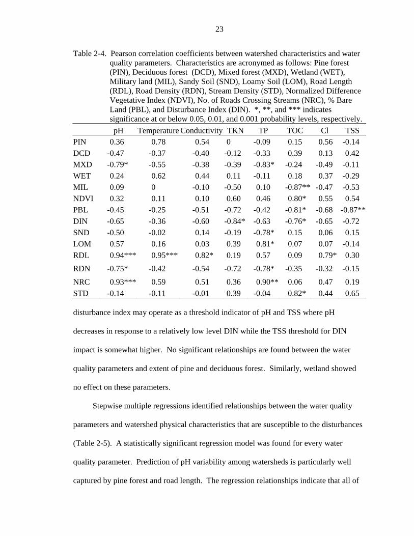
2-4. Pearson correlation coefficients between watershed characteristics and water quality parameters. ...................................................................................................23
2-5. Stepwise multiple regression models for water quality parameters. .........................24
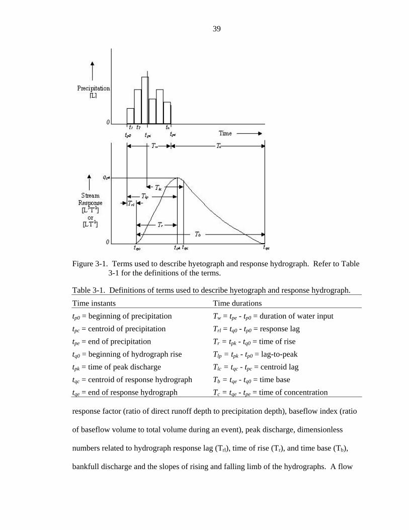
3-1. Definitions of terms used to describe hyetograph and response hydrograph. ...........39
3-2. Physical characteristics of study watersheds. ............................................................44
3-3. Summary of the recommended hydrologic indices for 'perennial runoff' type of streams......................................................................................................................46
3-4. Summary of hydrologic indices used in the Storm-Based Hydrologic Indices. ......49
3-5. Pearson correlation coefficients between watershed physical characteristics and event based hydrologic indices.. ..............................................................................53
3-6. Stepwise multiple regression models for event based hydrologic indices. . ...........54
4-1. REMM model parameters values by the riparian zone for the Bonham-South watershed in Fort Benning, Georgia. .......................................................................67
4-2. Soil and vegetation nutrient pools for Bonham-South watershed’s riparian area. ....69
4-3. Model simulated annual hydrologic budget for the riparian areas in Bonham-South watershed.. ......................................................................................69
4-4. Sensitivity of modeled streamflow and TKN based on +/- 10% change in model parameters for Bonham-South watershed. ...............................................................80
x
LIST OF FIGURES
Figure page 2-1 Study watersheds......................................................................................................14
2-2 Box plots of water quality parameters......................................................................20
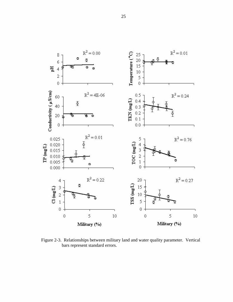
2-3 Relationships between military land and water quality parameter. .........................25
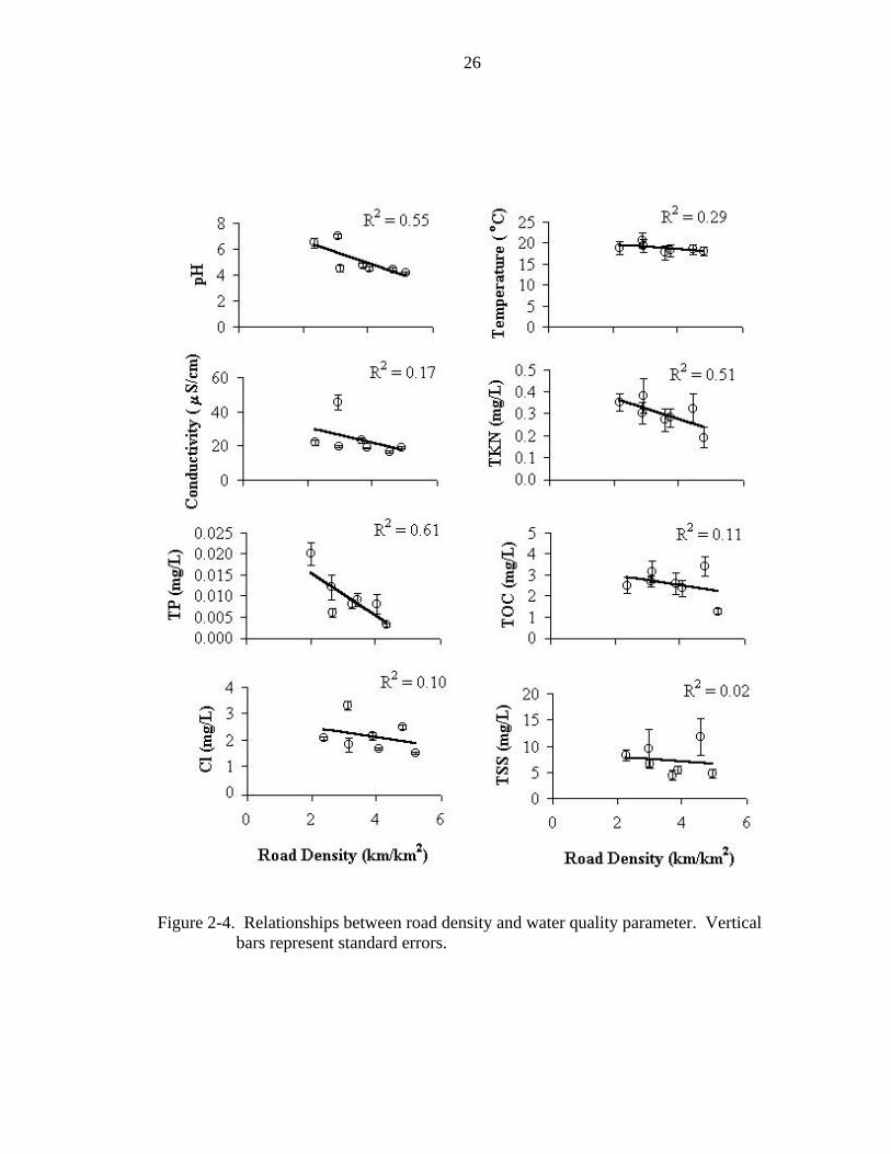
2-4 Relationships between road density and water quality parameter. ..........................26
2-5 Relationships between number of roads crossing streams and water quality parameter.. ................................................................................................................27
2-6 Relationships between disturbance index and water quality parameter...................28
3-1 Terms used to describe hyetograph and response hydrograph.................................39
3-2 Study watersheds......................................................................................................43
4-1 Study area.. ...............................................................................................................66
4-2. Comparison of REMM simulated daily flow with the observed daily flow for the Bonham-South watershed...................................................................................74
4-3. Observed canopy cover and TKN concentrations each month for the Bonham-South watershed. .......................................................................................75
4-4. Monthly simulated TKN concentration and simulated leaf mass in the Bonham-South’s riparian area.................................................................................................75
4-5. Monthly simulated TKN concentration and simulated nitrogen present in live leaves the Bonham-South’s riparian canopy. ...........................................................76
4-6. Observed TKN concentrations during the events......................................................78
4-7. Surface runoff comparison of the observed and simulated TKN masses..................79
4-8. Total streamflow comparison of the observed and simulated TKN masses..............79
xi
Abstract of Dissertation Presented to the Graduate School of the University of Florida in Partial Fulfillment of the Requirements for the Degree of Doctor of Philosophy
ECOHYDROLOGICAL STUDY OF WATERSHEDS WITHIN THE MILITARY INSTALLATION IN FORT BENNING, GEORGIA
By
Shirish Bhat
May 2005
Chair: Kirk Hatfield Cochair: Jennifer Jacobs Major Department: Civil and Coastal Engineering
Relationships among watershed physical characteristics and water quality
parameters were explored for seven watersheds in Fort Benning, Georgia, using statistical
analyses to identify chemical indicators of ecological changes. Correlations were
identified among the indicators and watershed physical characteristics. Regression
results suggested that pH, chloride, total phosphorus, total Kjeldahl nitrogen, total
organic carbon, and total suspended solids are useful indicators of watershed physical
characteristics that are susceptible to perturbations.
The magnitude, frequency, duration, timing, and rate of change of hydrologic
conditions regulate ecological processes in aquatic ecosystems. Analysis of 26 non-
redundant hydrologic indices showed undisturbed watershed produced higher magnitude
and more frequent low- and high-flows as compared to the disturbed watershed.
Eighteen storm-based indices, grouped into four flow components, were proposed to
statistically characterize hydrologic variation among different watersheds. Results

xii
showed that these storm-based indices might be used as surrogates to the indices derived
from long-term data. Statistical analysis showed that the watershed physical
characteristics such as military training land, road density, and the number of roads
crossing streams predicted hydrologic indices such as storm-based baseflow index,
bankfull discharge, response lag, and time of rise well.
Riparian vegetation has an important role in altering water quality in the forested
watersheds. The leaching of organic or mineral products on the forest floor provides
potential additional effects on water quality. In these areas, nutrients are released into the
fresh water systems due to the leaching and decomposition of vegetation litter. The
release of nutrients from plant litters prior to decomposition may be an important aspect
of characterizing stream water quality. To explore nitrogen leaching in a riparian area
during litterfall, Riparian Ecosystem Management Model developed by USDA-ARS has
been applied. The simulated total Kjeldahl nitrogen masses in the study watershed were
close to the observed values. The model effectively captured the trends of litter mass
accumulation in the riparian area and subsequent high concentrations and masses during
those periods.
1
CHAPTER 1 GENERAL INTRODUCTION
Ecohydrology is the interdisciplinary research field in which hydrology and
ecology come together. It may be defined as the study of the functional relations between
hydrology and biota at the watershed scale (Zalewski, 2000). Resource managers and
land use planners seek ecohydrological knowledge enabling them to design effective land
use plans and water management strategies.
Water, soil, and plant cover are fundamental components that determine the
productivity of the land. The successional stages in evolution of ecosystems depend on
climatic and hydrologic conditions and on nutrient availability. The unique composition
of plants and animals determines the ability to retain water and nutrients within the
system (Zalewski et al., 1997). The amount of water and its quality in the aquatic
environment are guided mostly by climate. Water and nutrient cycling in terrestrial
systems are tightly linked with each other and with human activity. The growth and
activity of human populations have increased the input of nutrients to terrestrial and
aquatic ecosystems (Schindler and Bayley, 1993; Vitousek et al., 1997). Various forms
of environmental perturbations affect quality and quantity of inland waters by increasing
runoff, erosion, sedimentation, and pollution.
Modifications of land use affect the water quality, residence time, surface runoff,
soil moisture, evaporation, and ground water. For example, an increase in urbanization
and non-forest land increased nitrogen concentration in the streams (Osborne and Wiley,
1988; Sponseller et al., 2001). Land-use practices can potentially affect and modify
2
channels along the flow paths in a landscape and may enhance or disrupt runoff
(Nakamura et al., 2000). Forest cutting can increase the frequency and volume of debris
slides due to dead and decayed tree roots that contribute to soil strength on marginally
stable sites (Sidle et al., 1985).
Water quality is highly variable, from place to place and from time to time, even
within a particular ecosystem. It is dependent on many factors, both natural and as a
consequence of human activities. In both cases, the quality of water is further affected by
the soils and vegetation over and through which it passes. Nutrients are released into the
freshwater systems due to the decomposition of the vegetation litter and modify the water
quality. Riparian vegetation has an important role in altering water quality as it functions
as a source or a sink of various organic and mineral components (Cirmo and McDonnell,
1997).
Agricultural practices and urbanization are widely recognized human impacts on
water resources. A specific type of human impact is caused at military installations.
Military training within a watershed can affect the drainage patterns, vegetation, and
soils. The impact is due to troop maneuvers and large tracked and wheeled vehicles that
traverse thousands of hectares in a single training exercise (Quist et al., 2003). The
impacts of such activities range from minor soil compaction and lodging of standing
vegetation to severe compaction and complete loss of vegetation cover in areas where
training is concentrated (Wilson, 1988; Milchunas et al., 1999). The resultant impacts are
evident both in the stream hydrology and the stream ecosystems. Potential impacts on
terrestrial and aquatic ecosystems include disruption in soil density and water content
(Helvey and Kochenderfer, 1990), addition of sediment, nutrients, and contaminants in
3
aquatic ecosystems (Gjessing et al., 1984), and impairment of natural habitat
development,and woody debris dynamics in forested floodplain streams (Piegay and
Landon, 1997). Military roads can significantly alter hillslope hydrology by
redistributing soil and rock materials on slopes and increasing the rate of debris slide
initiation. Roads also directly change the hydrology by intercepting shallow groundwater
flow paths, diverting the water along the roadway and routing it to stream at road
crossings. Road crossings can intercept groundwater drainage networks and collect
groundwater from upslope areas, diverting it into drainage ditches as surface water
(Wemple et al., 1996). Road crossings commonly found in military training areas may
act as barriers to the movement of fish and other aquatic habitats (Furniss et al., 1991).
Given the nature of military land use, management or military testing and training,
military land managers face the conflicting demands of balancing the primary military
mission with legal requirements to protect land and water quality (Milchunas et al.,
1999).
The military impacts can result in significant disruptions to the water and nutrient
cycles in the freshwater ecosystems and water resources. A few studies in the past have
addressed the effects of military training on terrestrial and aquatic ecosystems. For
example, Wilson (1988) found that the tank traffic resulted in a significant loss of native
species, increased abundance of introduced species, and increased bare soil at a training
site located in Manitoba. Milchunas et al. (1999) examined the effects of military
vehicles on plant communities and soil characteristics in Pinon Canyon Maneuver Site,
Colorado. Whitecotton et al. (2000) examined the impact of foot traffic from military
training on soil bulk density, infiltration rate, and aboveground biomass. Recently, Quist
4
et al. (2003) conducted a study in the Fort Riley Military Reservation, Kansas, to study
the effects of military use on terrestrial and aquatic communities.
Understanding human impacts in many landscapes needs the identification of
critical landscape elements and analysis of landscape pattern change (O’Neill et al.,
1997). Generalized response to military training includes the reduction in native and
perennial grasses, abundance of introduced species, and an increase in bare soil. Clearly,
these responses will alter biogeochemical and hydrological processes, which regulate
nutrient and water dynamics. However, impact of landscape changes to water quality and
stream is not well understood (Wand et al., 2001).
In order to maintain and improve water quality, there is an increasing need to
understand the relationships among watershed land use and stream ecosystems (Wang et
al., 2001). In parallel, perturbation induced effects on water quantity are critical to
stream ecology.
One of the many approaches to study the functional interrelations between the
hydrology and the stream biota is streamflow characterization and classification. This
approach develops hydrologic indices that account for characteristics of streamflow
variability that are biologically relevant (Olden and Poff, 2003). Characterization of
streams through development of ecologically relevant hydrologic indices is based on
long-term streamflow data. However, past studies overlooked the importance of storm-
flow data for the development of such hydrologic indices. Flow characteristics are
important where changes in land use are anticipated and where alterations to the flow
regimes need to be assessed.

5
The leaching of organic or mineral products from the forest floor provides potential
additional effects on water quality. Fluxes of nitrogen through the riparian zone are
intrinsically linked to water movement, both over and through the soil, and are also
strongly influenced by biological processes occurring in that zone. Nitrogen and organic
carbon dynamics in riparian zones are closely interrelated. While many of the factors
that can potentially influence nitrogen and carbon fluxes through riparian zones are
broadly known, there is presently incomplete quantitative information on the relative
importance of the flushing of nitrogen from freshly fallen leaves during precipitation
events.
Objectives
The United State’s Department of Defense (DOD) policy has established
ecosystem management as its approach to manage the military lands by maintaining and
improving the sustainability and biological diversity of terrestrial and freshwater
ecosystems while supporting human needs, including the DOD missions. In order to
identify critical deficiencies and research opportunities on ecosystem management
problems on defense installations, the Strategic Environmental Research and
Development Program (SERDP) of DOD initiated the SERDP Ecosystem Management
Program (SEMP) in December 1997. The objectives of SEMP were to (1) establish long-
term research sites on DOD lands for military-relevant ecosystem research, (2) conduct
ecosystem research and monitoring activities relevant to DOD requirements and
opportunities, and (3) facilitate the integration of results and findings of research into
DOD ecosystem management practices.
The goal of this research is to illustrate how an ecohydrological approach could be
used to advance our ability to predict the effects of anthropogenic perturbations on water-
6
vegetation-nutrient interactions in the military installation at Fort Benning, Georgia. The
issues addressed in this research encompass many of the main scientific challenges in the
military installations’ ecohydrology that include the effects of military related
perturbations on stream water quality and quantity, and the value of studying nutrient
dynamics in the riparian corridors of such regions. The specific objectives of this
research include (1) identification and examination of the statistical relationships among
water quality parameters and the watershed physical characteristics in low-nutrient
watersheds, (2) identification and development of hydrologic indices that characterize the
impact of military land management on watersheds, and (3) investigation of the effects of
nitrogen leaching from freshly fallen leaves on nutrient dynamics in a riparian area.
Dissertation Organization
Each chapter of this dissertation, except Chapters 1 and 5, is written as a self-
contained individual paper focusing on a topic that has not been addressed before.
Contributions are in the areas of water quality and land use within a military installation
(Chapter 2), development of storm-based hydrologic indices (Chapter 3), and watershed
scale nutrient leaching from a riparian area (Chapter 4). Chapter 5 summarizes and
concludes the research work
Chapter 2 is an original contribution in the effects of military activities related land
use on surface water quality. The major results from Chapter 2 are that the
concentrations of total organic carbon, total Kjeldahl nitrogen, total suspended solids, pH,
and total phosphorus in the stream show the greatest susceptibility to direct effects of
military activities. This chapter also identifies significant statistical relationships among
the water quality parameters and the military land uses. These relationships provide the

7
guidance for maintaining the surface water quality within the Fort Benning military
installation.
Chapter 3 is an original contribution in the ecohydrology that presents both annual-
based and storm-based methods for determining hydrologic indices that are of ecological
importance. Detailed descriptions of the methods for determining these indices and their
significance in aquatic ecosystems are described in this chapter. To statistically
characterize the hydrologic variation among different watersheds, 32 annual-based
hydrologic indices are analyzed. Eight out of 32 annual-based indices are recommended
to use for management practices within the Fort Benning military installation. As a new
approach to characterize the streamflow variability, 18 storm-based indices are proposed.
These indices are grouped into magnitude, frequency, duration, and rate of change of
flow. Storm-based indices are compared with annual-based indices. The storm-based
methodology provides guidance for measurements of appropriate indices within the
military installation.
Chapter 4 is an original contribution to the water quality function of the riparian
area. Nitrogen leaching from freshly fallen leaves in a riparian area during the
precipitation events is quantified. The observed nitrogen masses in the stream during the
precipitation events are compared with the model simulated values. Riparian Ecosystem
Management Model (REMM) is used to quantify the nitrogen in the riparian area. In this
chapter, details of the nitrogen leaching from the freshly fallen leaves are explored. The
results showed that the model effectively captured the trends of litter mass accumulation
in the riparian area and subsequent high concentrations during those periods. Analysis

8
showed that the simulated total Kjeldahl nitrogen masses during the precipitation events
were close to the observed masses.
Chapter 5 summarizes and concludes the research work. This chapter contains
recommendations to improve management of the water resources within the Fort Benning
military installation. Future research needs are also outlined in this chapter.

9
CHAPTER 2 ECOLOGICAL INDICATORS IN FORESTED WATERSHEDS IN FORT BENNING,
GEORGIA: RELATIONSHIP BETWEEN LAND USE AND STREAM WATER QUALITY
Introduction
Ecological monitoring is essential to protect ecological health and integrity. As
human activity alters land cover, degradation of water resources begins in the upland
areas of a watershed. The first step toward effective ecological monitoring and
assessment is to realize that the ultimate goal is to measure and evaluate the
consequences of human actions on ecological systems. Human activities that alter land
use eventually affect biogeochemical processes that influence water quality and alter
ecological processes.
The National Research Council of the United States recently conducted a critical
evaluation of indicators used to monitor ecological changes from either natural or
anthropogenic causes. During recent decades, efforts have been increasing to develop
reliable and comprehensive environmental indicators because of growing environmental
concerns (National Research Council, 2000). Indicators rapidly and effectively
communicate system status. Ecological indicators help to elucidate both the effects of
human activities and natural processes. They can also help to assess future implications
of these factors on ecosystem integrity. Once indicators identify areas or elements of the
environment that are under stress, successful management of problems can be measured
relative to both interim targets and long-term goals.

10
Indicators that relate key ecological responses to human perturbations provide
useful tools to better understand ecological effects and their monitoring and management.
A suite of indicators ranging from microbiologic to landscape metrics is necessary to
capture the full spatial, temporal, and ecological complexity of impacts (Dale et al.,
2002). Evaluation of representative indices across major physical gradients (e.g., soils,
geology, land use, water quality and quantity) can signal early environment change and
help diagnose the cause of an environmental problem.
Understanding human impacts in many landscapes needs the identification of
critical landscape elements and analysis of landscape pattern change (O’Neill et al.,
1997). Attention has refocused on relationships among watershed characteristics and
stream water quality (Johnson et al., 1997). In order to maintain and improve water
quality, there is an increasing need to understand the relationships among watershed land
use and stream ecosystems (Wang et al., 2001).
Land use provides information about ecosystem function and characterizes the
extent and diversity of ecosystem types. National Research Council (2000) has
recommended land use as one of the most effective indicators for ecological assessment.
Hydrologists and aquatic ecologists have long known that the pathway by which water
reaches to a stream or lake has a major effect on water quality. Early studies on the
physical (Harrel and Dorris, 1968) and chemical (Hynes, 1960) characteristics of
watersheds focused on the influence of geomorphic characteristics such as drainage area,
gradient, and stream order on turbidity, dissolved oxygen concentration, and temperature.
Many recent studies examine the influence of terrestrial ecosystems on stream or wetland
water quality (Richards and Host, 1994; Richards et al., 1997). Many other studies have
11
found relationships between land use and concentrations of nutrients in streams (e.g.,
Hunsaker and Levine, 1995; Johnes et al., 1996; Bolstad and Swank, 1997). Watershed
properties constrain in-stream physicochemical and biotic features. Richards et al. (1996)
showed that ecosystems could be influenced by land use at regional or broad geographic
scales. Osborne and Wiley (1988) found that the distance of urban land cover from the
stream effectively predicts stream nitrogen and phosphorus concentrations.
Within a military installation context, land managers are challenged to use the land
for military training purposes in a manner that is both ecologically sound and meets
military mission requirements (Garten Jr et al., 2003). Lands can suffer a slow
degradation if over-utilized by long-term human activities. The heavy vehicles used in
mechanized military training cause disturbance of soil structure and can change the
physical properties of the soil (Iverson et al., 1981). In rangelands, tracked vehicle traffic
affects the hydrological characteristics (Thurow et al., 1993). Trampled vegetation,
vehicle tracks through undisturbed area, and erosion caused by the overuse of trails are
some examples of the visible degradation to a landscape caused by military training
exercises. Few studies have developed predictive relationships among watershed
physical characteristics and surface water chemistry specific to military land use and low-
nutrient systems.
In the coastal plain of the Apalachicola-Chattahoochee-Flint (ACF) river basin,
cropland and silvicultural land in upland areas is separated from streams by relatively
undisturbed riparian flood plain and wetland habitats (Frick et al., 1998). This is in
contrast to many intensively farmed areas of the United States where wetlands have been
drained, channelized or filled, and little or no riparian buffers remain between cropland
12
and streams. Frick et al. (1998) reported that the lower nutrient concentrations in streams
within the ACF river basin could partially be attributed to wetland buffer areas, and
minimal use of pesticides as compared to other areas of the United States. Other studies
in the southeastern coastal plain watersheds (e.g., Lowrance 1984; Lowrance et al., 1992;
Perry et al., 1999; Fisher et al., 2000) focused primarily on the agricultural impacts, and
urbanization on stream water quality. The contribution of areas affected by military
training to nutrient discharges, specifically in Fort Benning watersheds, is yet to be
quantified.
This paper identifies and examines the statistical relationships among water quality
parameters and the watershed physical characteristics in seven low-nutrient watersheds
located in the Fort Benning military installation, Georgia. It is hypothesized that surface
water quality parameters can be used as indicators of ecological changes in watersheds.
Study Area
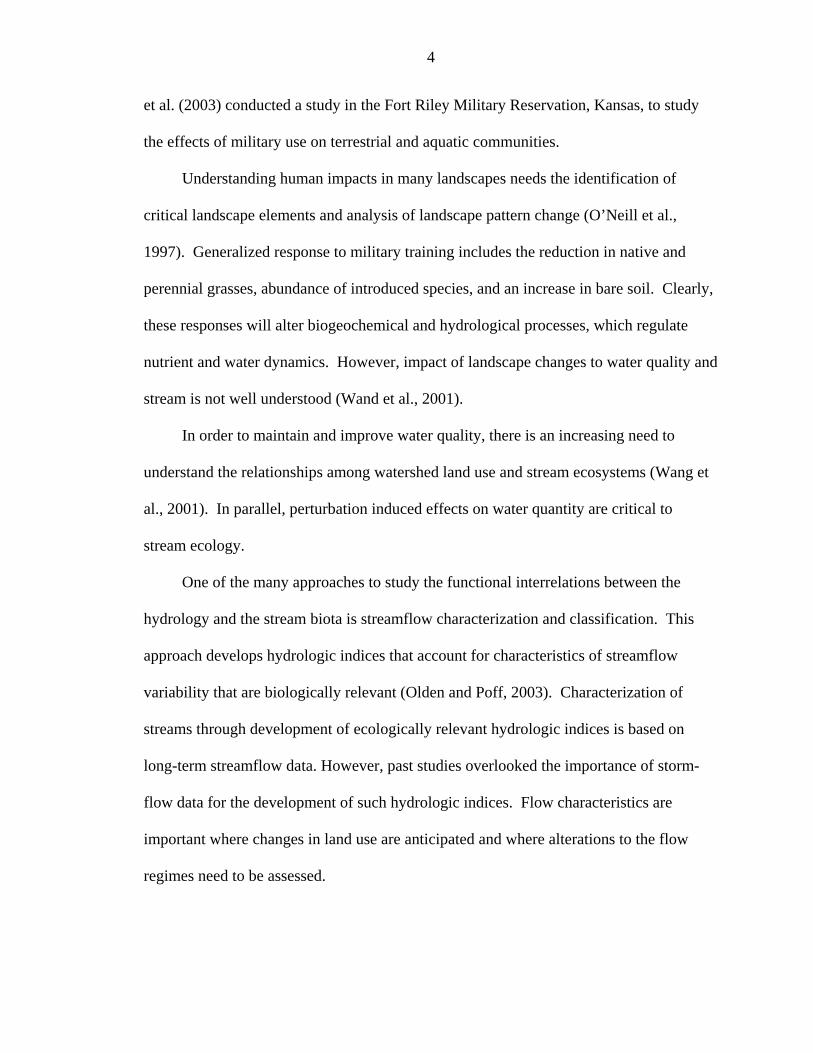
The Fort Benning Army Installation occupies approximately 73,503 ha in
Chattahoochee, Muscogee, and Marion Counties of Georgia and Russell County of
Alabama (Figure 2-1). The climate at Fort Benning is humid and mild. Rainfall in this
region occurs regularly throughout the year. July and August are the warmest months
with average daily maximum and minimum temperatures of 37 and 15oC. An average
daily maximum and minimum temperature of 15.5 and -1oC are reported in the coldest
months, January and February. Annual precipitation averages 1050 mm with October
being the driest month (Dale et al., 2002). Most of the precipitation occurs in the spring
and summer as a result of thunderstorms. Heavy rains are typical during the summer but
can occur in any month. Snow accounts for less than 1% of the annual precipitation.
13
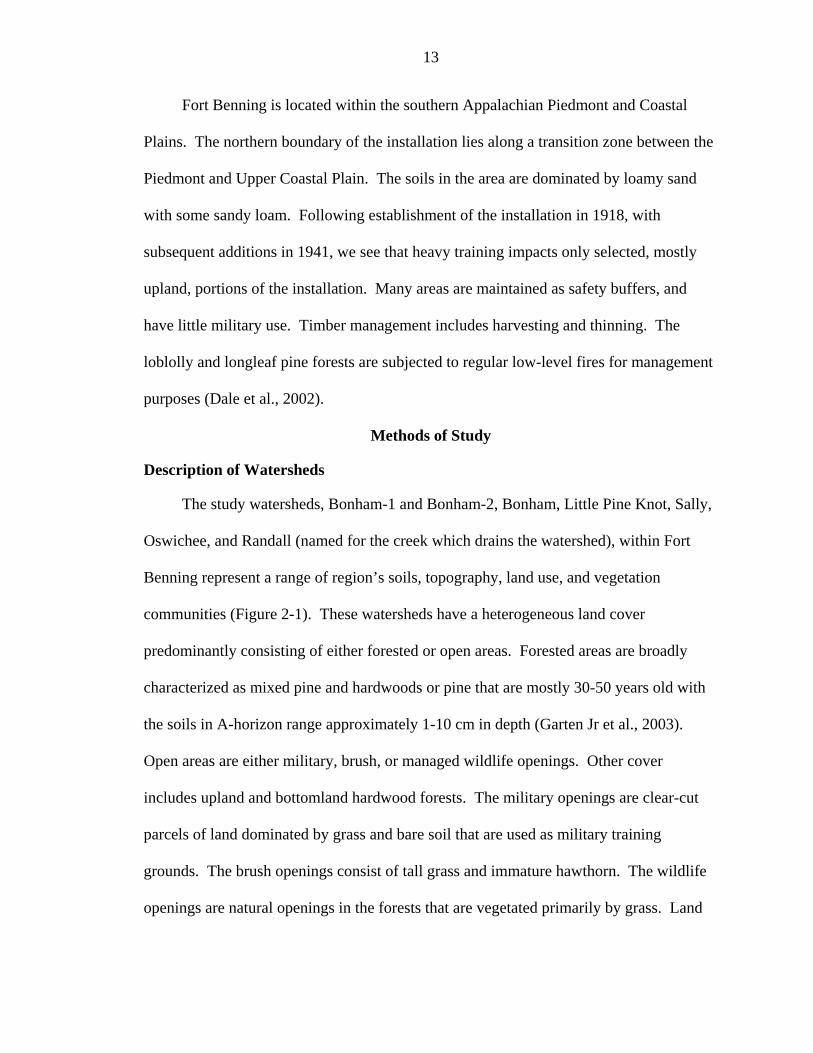
Fort Benning is located within the southern Appalachian Piedmont and Coastal
Plains. The northern boundary of the installation lies along a transition zone between the
Piedmont and Upper Coastal Plain. The soils in the area are dominated by loamy sand
with some sandy loam. Following establishment of the installation in 1918, with
subsequent additions in 1941, we see that heavy training impacts only selected, mostly
upland, portions of the installation. Many areas are maintained as safety buffers, and
have little military use. Timber management includes harvesting and thinning. The
loblolly and longleaf pine forests are subjected to regular low-level fires for management
purposes (Dale et al., 2002).
Methods of Study
Description of Watersheds
The study watersheds, Bonham-1 and Bonham-2, Bonham, Little Pine Knot, Sally,
Oswichee, and Randall (named for the creek which drains the watershed), within Fort
Benning represent a range of region’s soils, topography, land use, and vegetation
communities (Figure 2-1). These watersheds have a heterogeneous land cover
predominantly consisting of either forested or open areas. Forested areas are broadly
characterized as mixed pine and hardwoods or pine that are mostly 30-50 years old with
the soils in A-horizon range approximately 1-10 cm in depth (Garten Jr et al., 2003).
Open areas are either military, brush, or managed wildlife openings. Other cover
includes upland and bottomland hardwood forests. The military openings are clear-cut
parcels of land dominated by grass and bare soil that are used as military training
grounds. The brush openings consist of tall grass and immature hawthorn. The wildlife
openings are natural openings in the forests that are vegetated primarily by grass. Land
14
impacts due to heavy military activities (e.g., infantry, artillery, wheeled, and tracked
vehicle training) occur only in selected portions in these watersheds.
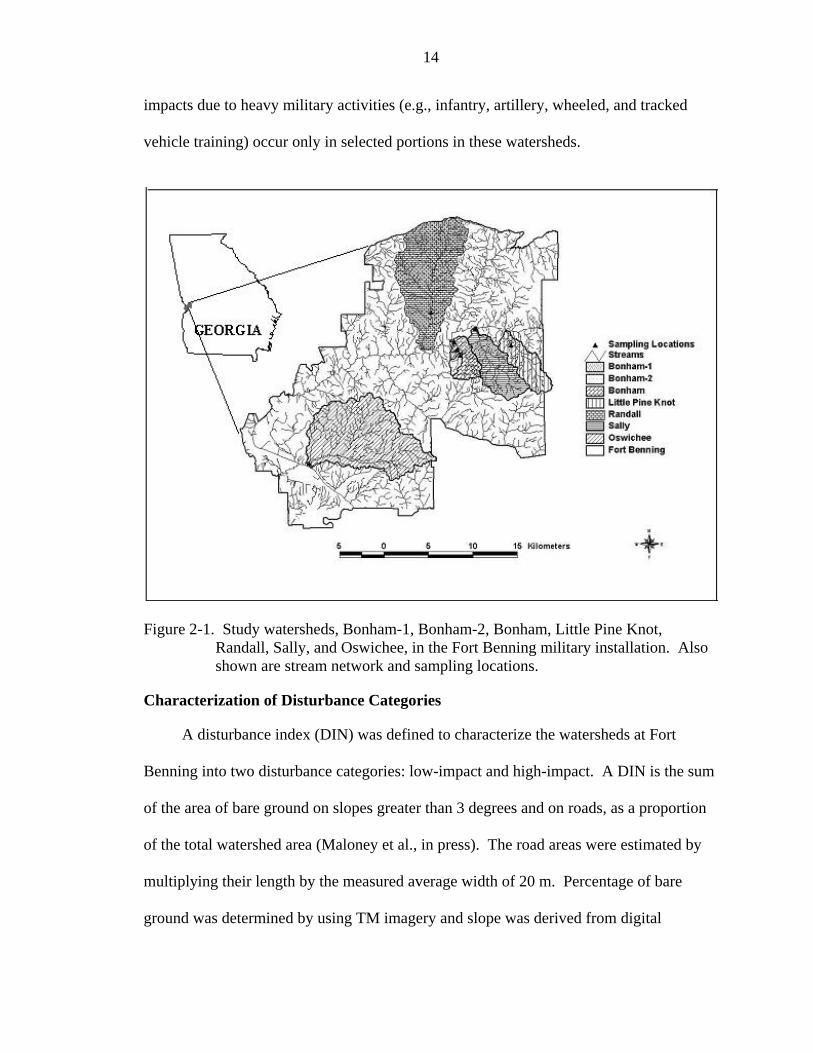
Figure 2-1. Study watersheds, Bonham-1, Bonham-2, Bonham, Little Pine Knot,
Randall, Sally, and Oswichee, in the Fort Benning military installation. Also shown are stream network and sampling locations.
Characterization of Disturbance Categories
A disturbance index (DIN) was defined to characterize the watersheds at Fort
Benning into two disturbance categories: low-impact and high-impact. A DIN is the sum
of the area of bare ground on slopes greater than 3 degrees and on roads, as a proportion
of the total watershed area (Maloney et al., in press). The road areas were estimated by
multiplying their length by the measured average width of 20 m. Percentage of bare
ground was determined by using TM imagery and slope was derived from digital
15
elevation maps. The TM imagery and digital elevation maps were obtained from
Strategic Environmental Research and Development Plan (SERDP)’s Ecosystem
Management Project (SEMP) database. Watersheds having a disturbance index from 0 to
11% are designated as low-impacted watersheds. High-impacted watersheds have
disturbance indices greater than or equal to 11%.
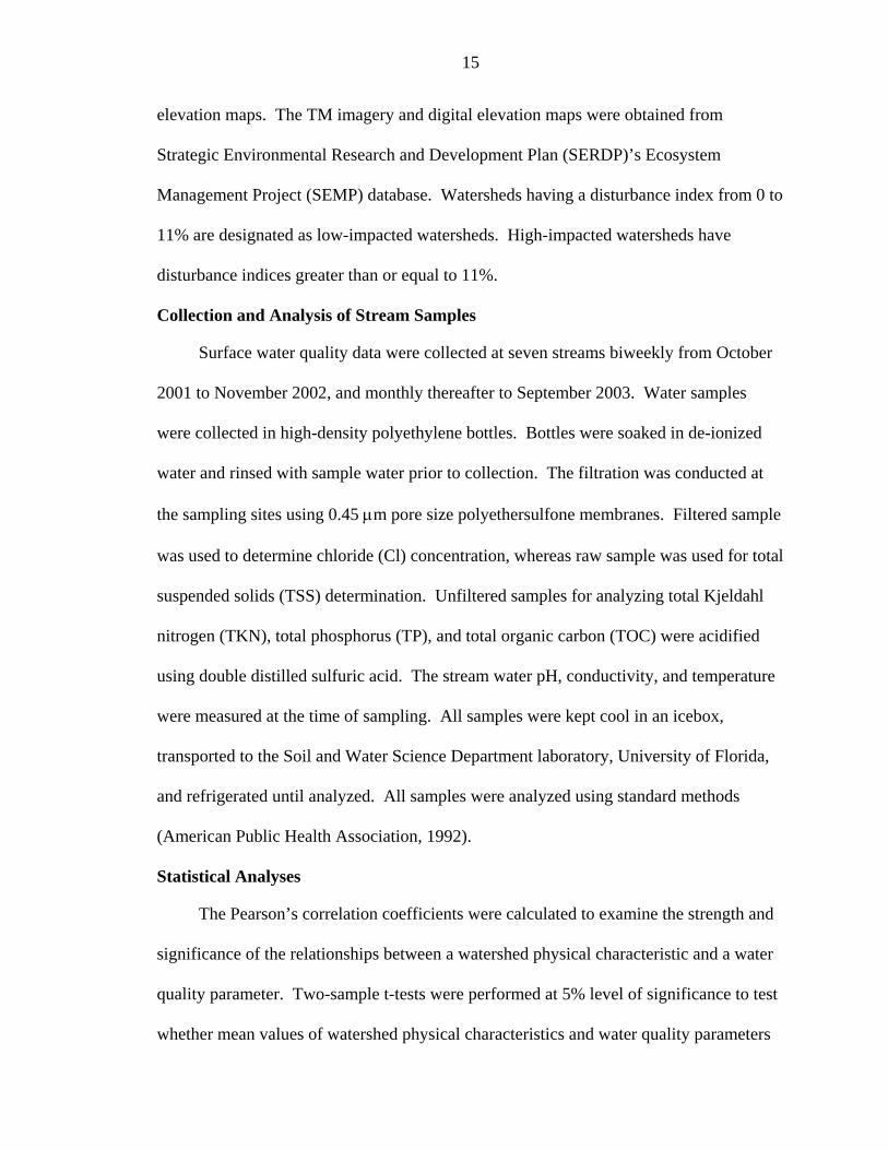
Collection and Analysis of Stream Samples
Surface water quality data were collected at seven streams biweekly from October
2001 to November 2002, and monthly thereafter to September 2003. Water samples
were collected in high-density polyethylene bottles. Bottles were soaked in de-ionized
water and rinsed with sample water prior to collection. The filtration was conducted at
the sampling sites using 0.45 µm pore size polyethersulfone membranes. Filtered sample
was used to determine chloride (Cl) concentration, whereas raw sample was used for total
suspended solids (TSS) determination. Unfiltered samples for analyzing total Kjeldahl
nitrogen (TKN), total phosphorus (TP), and total organic carbon (TOC) were acidified
using double distilled sulfuric acid. The stream water pH, conductivity, and temperature
were measured at the time of sampling. All samples were kept cool in an icebox,
transported to the Soil and Water Science Department laboratory, University of Florida,
and refrigerated until analyzed. All samples were analyzed using standard methods
(American Public Health Association, 1992).
Statistical Analyses
The Pearson’s correlation coefficients were calculated to examine the strength and
significance of the relationships between a watershed physical characteristic and a water
quality parameter. Two-sample t-tests were performed at 5% level of significance to test
whether mean values of watershed physical characteristics and water quality parameters

16
differ between low- and high-disturbance watersheds. Characteristics showing
significant correlations with a water quality parameter were considered for stepwise
multiple linear regression models. Only variables having less than or equal to 0.05
significance level were retained in the regression models.
Results
Watershed Physical Characteristics
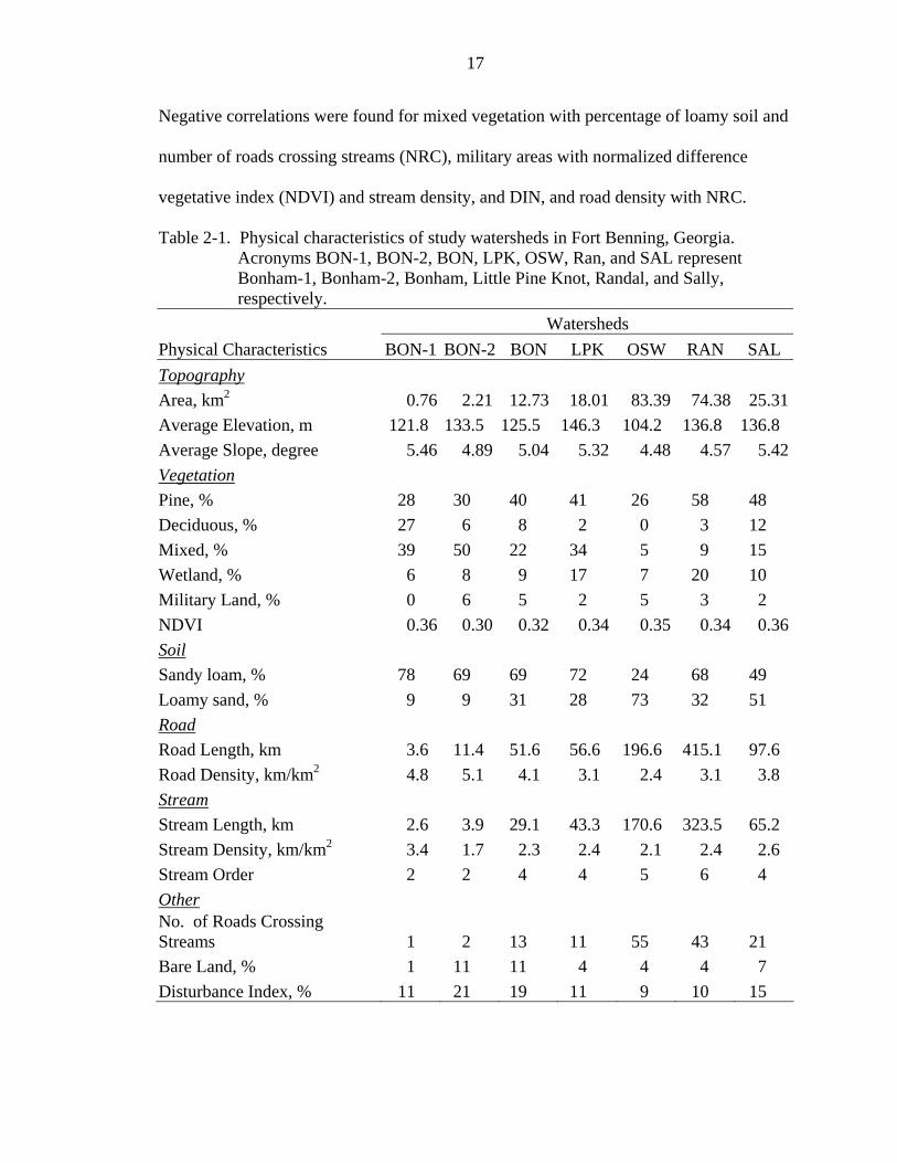
The watersheds’ physical characteristics are summarized in Table 2-1. Most of the
watersheds are highly vegetated (70% or more) except Oswichee (38%) with the majority
characterized by pine and mixed pine and hardwoods. Deciduous forest typically covers
only a small percentage of these watersheds. However, Bonham-1 consists of 27% of
deciduous forest. The study watersheds range from less than 1 to 84 km2. The
topographic characteristics of study watersheds are typical of forested watersheds of
southeastern coastal plain (Lowrance, 1992; Perry et al., 1999). Average elevations vary
from 104 to 148 m above mean sea level. Maximum slopes vary from 4 to 6 degrees.
Sandy soils are common in most of the study watersheds. However, loamy soils cover
most of the Sally and Oswichee watersheds. Bottomlands comprise 6 to 20% of the
watershed. The military training extent (0 to 6%) is relatively small. Total bare lands in
these watersheds comprise 9 to 21% of the watershed area, of which 1 to 8% of the total
area is unpaved roads and trails. This extent and variability of military training and bare
land are typical of the entire Fort Benning installation.
Some watershed characteristics are strongly correlated at significance level of 0.05
or lower (Table 2-2). Significant positive correlations exist for pine with the bottomland
wetlands, deciduous vegetation with stream density, number of roads crossing streams
with road length and percent of loam, and disturbance index with percent bare land.
17
Negative correlations were found for mixed vegetation with percentage of loamy soil and
number of roads crossing streams (NRC), military areas with normalized difference
vegetative index (NDVI) and stream density, and DIN, and road density with NRC.
Table 2-1. Physical characteristics of study watersheds in Fort Benning, Georgia. Acronyms BON-1, BON-2, BON, LPK, OSW, Ran, and SAL represent Bonham-1, Bonham-2, Bonham, Little Pine Knot, Randal, and Sally, respectively.
Watersheds Physical Characteristics BON-1 BON-2 BON LPK OSW RAN SAL Topography Area, km2 0.76 2.21 12.73 18.01 83.39 74.38 25.31Average Elevation, m 121.8 133.5 125.5 146.3 104.2 136.8 136.8 Average Slope, degree 5.46 4.89 5.04 5.32 4.48 4.57 5.42Vegetation Pine, % 28 30 40 41 26 58 48 Deciduous, % 27 6 8 2 0 3 12 Mixed, % 39 50 22 34 5 9 15 Wetland, % 6 8 9 17 7 20 10 Military Land, % 0 6 5 2 5 3 2 NDVI 0.36 0.30 0.32 0.34 0.35 0.34 0.36Soil Sandy loam, % 78 69 69 72 24 68 49 Loamy sand, % 9 9 31 28 73 32 51 Road Road Length, km 3.6 11.4 51.6 56.6 196.6 415.1 97.6 Road Density, km/km2 4.8 5.1 4.1 3.1 2.4 3.1 3.8 Stream Stream Length, km 2.6 3.9 29.1 43.3 170.6 323.5 65.2 Stream Density, km/km2 3.4 1.7 2.3 2.4 2.1 2.4 2.6 Stream Order 2 2 4 4 5 6 4 Other No. of Roads Crossing Streams 1 2 13 11 55 43 21 Bare Land, % 1 11 11 4 4 4 7 Disturbance Index, % 11 21 19 11 9 10 15
18
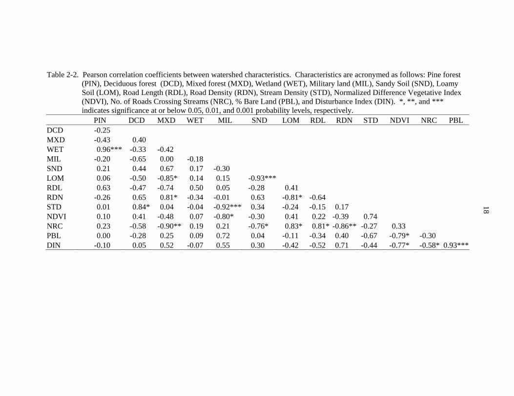
Table 2-2. Pearson correlation coefficients between watershed characteristics. Characteristics are acronymed as follows: Pine forest (PIN), Deciduous forest (DCD), Mixed forest (MXD), Wetland (WET), Military land (MIL), Sandy Soil (SND), Loamy Soil (LOM), Road Length (RDL), Road Density (RDN), Stream Density (STD), Normalized Difference Vegetative Index (NDVI), No. of Roads Crossing Streams (NRC), % Bare Land (PBL), and Disturbance Index (DIN). *, **, and *** indicates significance at or below 0.05, 0.01, and 0.001 probability levels, respectively.
PIN DCD MXD WET MIL SND LOM RDL RDN STD NDVI NRC PBL DCD -0.25 MXD -0.43 0.40 WET 0.96*** -0.33 -0.42 MIL -0.20 -0.65 0.00 -0.18 SND 0.21 0.44 0.67 0.17 -0.30 LOM 0.06 -0.50 -0.85* 0.14 0.15 -0.93*** RDL 0.63 -0.47 -0.74 0.50 0.05 -0.28 0.41 RDN -0.26 0.65 0.81* -0.34 -0.01 0.63 -0.81* -0.64 STD 0.01 0.84* 0.04 -0.04 -0.92*** 0.34 -0.24 -0.15 0.17 NDVI 0.10 0.41 -0.48 0.07 -0.80* -0.30 0.41 0.22 -0.39 0.74 NRC 0.23 -0.58 -0.90** 0.19 0.21 -0.76* 0.83* 0.81* -0.86** -0.27 0.33 PBL 0.00 -0.28 0.25 0.09 0.72 0.04 -0.11 -0.34 0.40 -0.67 -0.79* -0.30 DIN -0.10 0.05 0.52 -0.07 0.55 0.30 -0.42 -0.52 0.71 -0.44 -0.77* -0.58* 0.93***
19
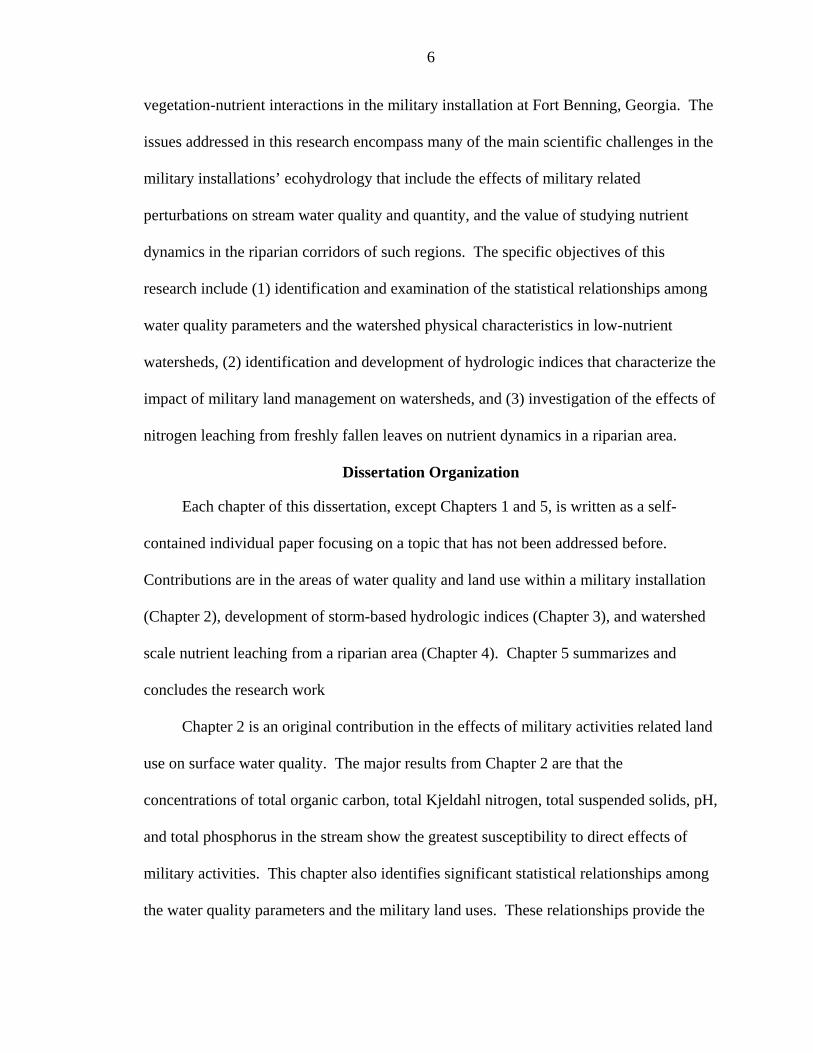
Water Quality Parameters
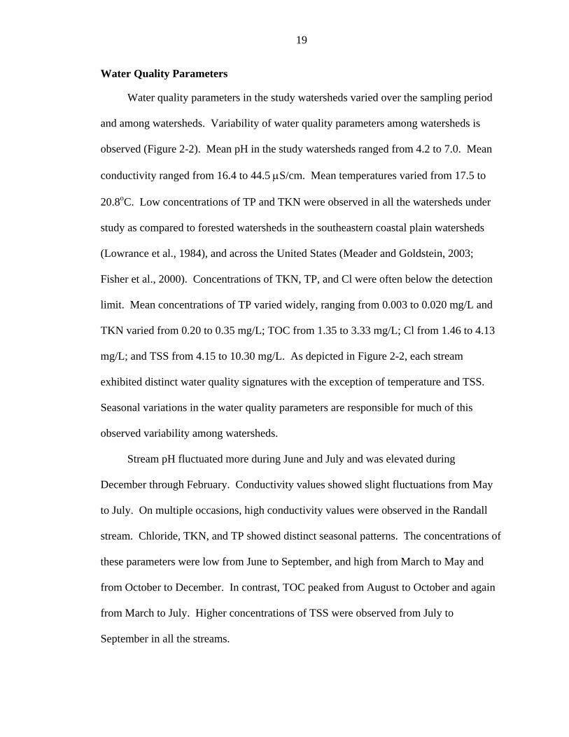
Water quality parameters in the study watersheds varied over the sampling period
and among watersheds. Variability of water quality parameters among watersheds is
observed (Figure 2-2). Mean pH in the study watersheds ranged from 4.2 to 7.0. Mean
conductivity ranged from 16.4 to 44.5 µS/cm. Mean temperatures varied from 17.5 to
20.8oC. Low concentrations of TP and TKN were observed in all the watersheds under
study as compared to forested watersheds in the southeastern coastal plain watersheds
(Lowrance et al., 1984), and across the United States (Meader and Goldstein, 2003;
Fisher et al., 2000). Concentrations of TKN, TP, and Cl were often below the detection
limit. Mean concentrations of TP varied widely, ranging from 0.003 to 0.020 mg/L and
TKN varied from 0.20 to 0.35 mg/L; TOC from 1.35 to 3.33 mg/L; Cl from 1.46 to 4.13
mg/L; and TSS from 4.15 to 10.30 mg/L. As depicted in Figure 2-2, each stream
exhibited distinct water quality signatures with the exception of temperature and TSS.
Seasonal variations in the water quality parameters are responsible for much of this
observed variability among watersheds.
Stream pH fluctuated more during June and July and was elevated during
December through February. Conductivity values showed slight fluctuations from May
to July. On multiple occasions, high conductivity values were observed in the Randall
stream. Chloride, TKN, and TP showed distinct seasonal patterns. The concentrations of
these parameters were low from June to September, and high from March to May and
from October to December. In contrast, TOC peaked from August to October and again
from March to July. Higher concentrations of TSS were observed from July to
September in all the streams.
20
Figure 2-2. Box plots of water quality parameters. Each plot consists of outliers, most
extreme data, 75th, 50th, and 25th percentile values. Watershed IDs represent- 1: Bonham-1, 2: Randall, 3: Oswichee, 4: Little Pine Knot, 5: Sally, 6: Bonham, and 7: Bonham-2.
21
Effects of Disturbance Categories
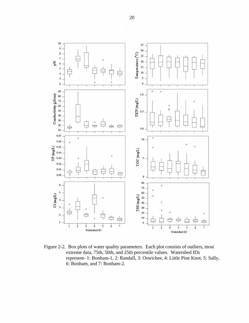
Table 2-3 presents the t-test results of the comparison of physical characteristics
and water quality parameters based on the watershed disturbance level. The only
physical characteristic having a significant difference (α = 0.04) between these two
groups was DIN. While the low-impact watersheds tended to have higher chemical
Table 2-3. t-test results for differences in mean values of watershed physical characteristics and water quality parameters. * indicates significance at or below 0.05 probability level. NS indicates non-significant difference at the 0.05 probability level.
Low-Impacted High-Impacted Mean SD Mean SD Watershed Characteristics Pine, % 38.3 14.8 39.3 9.0 NS Deciduous, % 8.0 12.7 8.7 3.1 NS Mixed, % 21.8 17.2 29 18.5 NS Wetland, % 14.5 9.5 16 7.2 NS Military Land, % 2.4 2.0 4.3 2.3 NS Sand, % 60.5 24.7 62.3 11.5 NS Loam, % 35.5 26.9 30.3 21.0 NS NDVI 0.35 0.01 0.32 0.03 NS Road Length, km 168 184 53.5 43.2 NS
Road Density, km/km2 3.3 1.0 4.3 0.7 NS
Stream Density, km/km2 2.6 0.6 2.2 0.4 NS No. of Roads Crossing Streams 27.5 25.6 12 9.5 NS Disturbance Index, % 10.2 0.9 18.3 3.1 * Water Quality Parameters pH 5.6 1.3 4.5 0.3 NS
Temperature, oC 19.3 0.9 18 0.3 NS Conductivity, µS/cm 25.9 13.3 20.4 2.5 NS TKN, mg/L 0.3 0.03 0.2 0.05 NS TP, mg/L 0.011 0.006 0.007 0.003 NS TOC, mg/L 2.9 0.4 2.1 0.7 NS Cl, mg/L 2.4 0.5 1.8 0.3 NS TSS, mg/L 9.1 2.2 4.8 0.5 *

22
concentrations than the high-impact watersheds, only TSS showed significant difference
(α = 0.03). Even though the results showed no significant statistical differences at a
confidence level of 95%, the t-test results of all water quality parameters, except
conductivity and TP, showed significant differences at 80% confidence interval between
high- and low-impacted watersheds. The relatively small sample size and natural
variability among watersheds may have limited the ability to discern significance
differences.
Relationship between Watershed Physical Characteristics and Water Quality Parameters
Correlation and regression analyses were performed to identify relationships among
the watershed physical characteristics and the water quality parameters. Table 2-4 shows
that each water quality parameter had a significant relationship with one or more
watershed physical characteristics (Table 2-4). The correlation results show that
decreasing mixed vegetation increased pH and TP. Sandy and loamy soils had opposite
effects on TP. An increase in sandy soil decreased TP, whereas an increase in loamy soil
increased TP. Increasing military land decreased TOC. Temperature, pH, conductivity,
and Cl increased as the road length increased. The number of roads crossing streams had
positive correlations on pH and TP. Percent bare land was negatively correlated with
TOC and TSS. Disturbance index was negatively correlated with TKN and TOC.
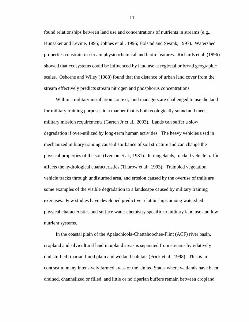
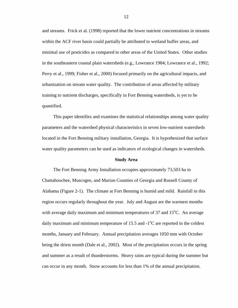
Graphical relationships provide insight into nonlinear relationships that exist
between indicators and response variables. Figures 2-3 to 2-6 show some of the most
striking relationships between watershed characteristics directly and/or indirectly affected
by management of military lands and their effect on water chemistry. As the % military
land increases, the TKN, TOC, and TSS decrease in a linear fashion. However,
23
Table 2-4. Pearson correlation coefficients between watershed characteristics and water quality parameters. Characteristics are acronymed as follows: Pine forest (PIN), Deciduous forest (DCD), Mixed forest (MXD), Wetland (WET), Military land (MIL), Sandy Soil (SND), Loamy Soil (LOM), Road Length (RDL), Road Density (RDN), Stream Density (STD), Normalized Difference Vegetative Index (NDVI), No. of Roads Crossing Streams (NRC), % Bare Land (PBL), and Disturbance Index (DIN). *, **, and *** indicates significance at or below 0.05, 0.01, and 0.001 probability levels, respectively.
pH Temperature Conductivity TKN TP TOC Cl TSS PIN 0.36 0.78 0.54 0 -0.09 0.15 0.56 -0.14 DCD -0.47 -0.37 -0.40 -0.12 -0.33 0.39 0.13 0.42 MXD -0.79* -0.55 -0.38 -0.39 -0.83* -0.24 -0.49 -0.11 WET 0.24 0.62 0.44 0.11 -0.11 0.18 0.37 -0.29 MIL 0.09 0 -0.10 -0.50 0.10 -0.87** -0.47 -0.53 NDVI 0.32 0.11 0.10 0.60 0.46 0.80* 0.55 0.54 PBL -0.45 -0.25 -0.51 -0.72 -0.42 -0.81* -0.68 -0.87**DIN -0.65 -0.36 -0.60 -0.84* -0.63 -0.76* -0.65 -0.72 SND -0.50 -0.02 0.14 -0.19 -0.78* 0.15 0.06 0.15 LOM 0.57 0.16 0.03 0.39 0.81* 0.07 0.07 -0.14 RDL 0.94*** 0.95*** 0.82* 0.19 0.57 0.09 0.79* 0.30
RDN -0.75* -0.42 -0.54 -0.72 -0.78* -0.35 -0.32 -0.15
NRC 0.93*** 0.59 0.51 0.36 0.90** 0.06 0.47 0.19 STD -0.14 -0.11 -0.01 0.39 -0.04 0.82* 0.44 0.65 disturbance index may operate as a threshold indicator of pH and TSS where pH
decreases in response to a relatively low level DIN while the TSS threshold for DIN
impact is somewhat higher. No significant relationships are found between the water
quality parameters and extent of pine and deciduous forest. Similarly, wetland showed
no effect on these parameters.
Stepwise multiple regressions identified relationships between the water quality
parameters and watershed physical characteristics that are susceptible to the disturbances
(Table 2-5). A statistically significant regression model was found for every water
quality parameter. Prediction of pH variability among watersheds is particularly well
captured by pine forest and road length. The regression relationships indicate that all of
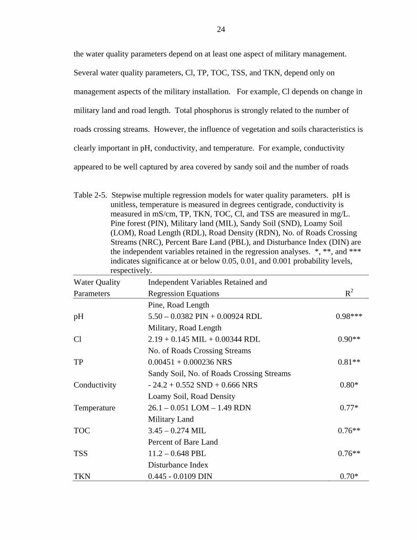
24
the water quality parameters depend on at least one aspect of military management.
Several water quality parameters, Cl, TP, TOC, TSS, and TKN, depend only on
management aspects of the military installation. For example, Cl depends on change in
military land and road length. Total phosphorus is strongly related to the number of
roads crossing streams. However, the influence of vegetation and soils characteristics is
clearly important in pH, conductivity, and temperature. For example, conductivity
appeared to be well captured by area covered by sandy soil and the number of roads
Table 2-5. Stepwise multiple regression models for water quality parameters. pH is
unitless, temperature is measured in degrees centigrade, conductivity is measured in mS/cm, TP, TKN, TOC, Cl, and TSS are measured in mg/L. Pine forest (PIN), Military land (MIL), Sandy Soil (SND), Loamy Soil (LOM), Road Length (RDL), Road Density (RDN), No. of Roads Crossing Streams (NRC), Percent Bare Land (PBL), and Disturbance Index (DIN) are the independent variables retained in the regression analyses. *, **, and *** indicates significance at or below 0.05, 0.01, and 0.001 probability levels, respectively.
Water Quality Independent Variables Retained and Parameters Regression Equations R2 Pine, Road Length pH 5.50 – 0.0382 PIN + 0.00924 RDL 0.98*** Military, Road Length Cl 2.19 + 0.145 MIL + 0.00344 RDL 0.90** No. of Roads Crossing Streams TP 0.00451 + 0.000236 NRS 0.81** Sandy Soil, No. of Roads Crossing Streams Conductivity - 24.2 + 0.552 SND + 0.666 NRS 0.80* Loamy Soil, Road Density Temperature 26.1 – 0.051 LOM – 1.49 RDN 0.77* Military Land TOC 3.45 – 0.274 MIL 0.76** Percent of Bare Land TSS 11.2 – 0.648 PBL 0.76** Disturbance Index TKN 0.445 - 0.0109 DIN 0.70*
25
Figure 2-3. Relationships between military land and water quality parameter. Vertical
bars represent standard errors.
26
Figure 2-4. Relationships between road density and water quality parameter. Vertical
bars represent standard errors.
27
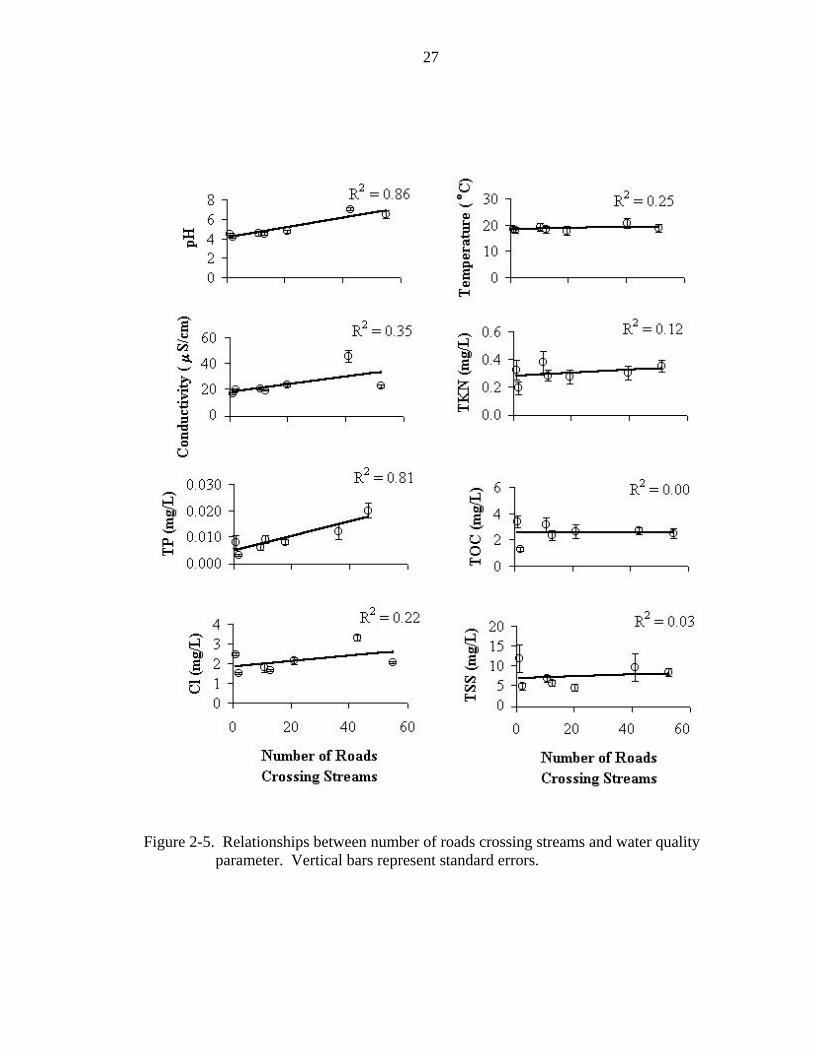
Figure 2-5. Relationships between number of roads crossing streams and water quality
parameter. Vertical bars represent standard errors.
28
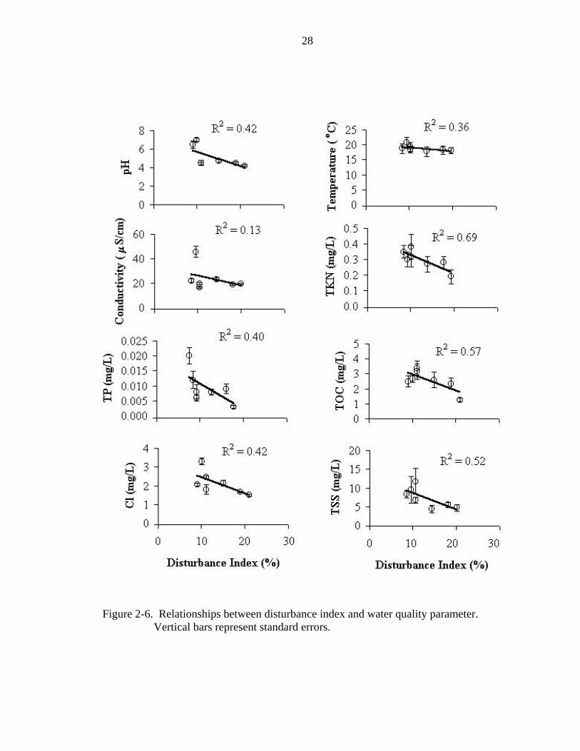
Figure 2-6. Relationships between disturbance index and water quality parameter.
Vertical bars represent standard errors.

29
crossing streams, whereas temperature was captured by loamy sand soil and road density.
Overall, the regression models show that it is possible to quantify the effects of watershed
physical characteristics on the water quality parameters.
Discussion
Variations in stream water chemistry among the study watersheds reflect
differences in biogeochemical reactions occurring in the watersheds. The results of this
study indicate that even in low impact watersheds, physical characteristics may be used to
explain variations in stream water chemistry and, by inference, the relative watershed
disturbance levels. The observed variability in many of the chemical parameters studied
in these watersheds can be attributed to physical characteristics of the watersheds or land
management patterns within the watersheds as evidenced by the road network, forestry
practices, and military training.
Diverse human activities interact to affect conditions in watersheds and water
bodies. Sites of interest can be grouped and placed on a gradient according to activities
and their effects. The results of this study suggest that the vegetation type, road length,
number of roads crossing streams, and disturbance index are important predictors of
water quality variability. Vegetation cover was related to stream pH and TP (mixed
forest) and conductivity (pine forest). However, deciduous forest cover was not related
to any of the water quality parameters suggesting a limited effect in organic matter and
nutrient production and variability as observed among Fort Benning watersheds.
However some other subtle landscape changes resulted in relatively larger impacts on
water quality parameters. Low-impact watersheds tend to produce higher concentrations
of nutrients in the streams. This can be attributed to the availability of more soil organic
30
matter and the rapid biogeochemical processes occurring in the low-impact watersheds as
compared to the high-impact watersheds.
It is extremely difficult to capture all aspects of human influence in a single graph
or statistical test. However, sometimes meaningful chemical patterns can be lost by
excessive dependence on the outcome of menu-driven statistical tests (Karr and Chu,
1999). Figures 2-3 to 2-6 depict several different aspects of stream’s chemical conditions
against several measures of human influences, such as military land use, disturbance
index, number of roads crossing streams, and road density. The distribution of circles in
most of these figures illustrate that a chemical metric indicates little about a condition
simply because it does not correlate strongly with a single surrogate of that condition.
However, where the relationship between human influence and stream’s chemical
response is strong, statistics and graph agree.
The correlation tests identify linear relationships between a chemical response and
watershed characteristics. Weak statistical correlations observed in these analyses may
have missed important chemical patterns. For example, nonlinear patterns were observed
for forest types, bare land (not shown here), and disturbance index (Figure 2-6). The
plots in Figure 2-6 show a step-function for TSS and pH. The scatter of this dataset
shows little or no statistical significance, but can be interpreted chemically. For TSS,
those watersheds having a disturbance index of 11% or lower had a higher level than
those with a greater disturbance index.
When a number of variables interact to influence water quality conditions, it may
be difficult to explain observed variability in a single plot against one dimension of
human influence (Figure 2-4). Chemical responses were plotted against the road
31
densities for various watersheds. The Pearson correlation coefficient for TP was
significant capturing human influence on this chemical parameter. The response of TP is
visibly distinguished from others. A similar discussion is true for military land with TOC
(Figure 2-3); number of roads crossing streams with pH and TP (Figure 2-5); and
disturbance index with TKN (Figure 2-6).
The relationships between water quality parameters and physical characteristics
indicate that disturbances in low nutrient forested environments decrease some chemical
signatures. Watersheds with more roads, e.g., Randall and Oswichee, have relatively
high pH, conductivity, and Cl compared to the watersheds with fewer roads. Watersheds
with a small portion of military land, e.g., Bonham-1, Sally, and Little Pine Knot, have
relatively high TOC concentrations. In contrast, watersheds characterized by higher road
densities, e.g., Bonham and Bonham-2, had low TP concentrations. Higher disturbance
index, similar to the road density, showed lower TKN and TOC concentrations in the
streams. Mixed vegetation, road length, percent of bare land, DIN, and number of roads
crossing streams were able to capture most of the variability in water quality parameters.
In a watershed scale study conducted in Ontario, Canada, Sliva and Williams
(2001) found a negative correlation of forested land cover with TSS and chloride. In
contrast, Johnson et al. (1997) showed a positive relationship of forest with TSS in a
study of landscape influence on water chemistry in the Saginaw Bay watershed of central
Michigan. Johnson et al.’s (1997) results indicated that row crop agriculture had the
highest effect on total nitrogen, nitrate, and total dissolved solids. They also observed
that urban and forest areas were positively correlated good predictors of TSS, whereas
row crop agriculture was positively correlated with total nitrogen. Basnyat et al. (1999)
32
reported a positive association of TSS with agricultural practices in the Fish River
watershed, Alabama. The Fort Benning installation is characterized by relatively low
variability in forest cover and suggests, in contrast to other studies, that neither TSS nor
Cl may be related to forest cover under existing land management practices. Instead,
Fort Benning’s road extent and percent bare land are better predictors of TSS and Cl.
Most studies identified urban land use as a dominant factor causing elevated total
nitrogen and nitrate concentrations in the streams (Hill, 1981; Osborne and Wiley, 1988).
Sponseller et al. (2001) found positive correlation of total inorganic nitrogen with
percentage of non-forested land in southwestern Virginia watersheds. A negative
correlation of TKN to DIN, in this study, is consistent with studies (e.g., Sponseller et al.,
2001; Hunsaker and Levine, 1995; Johnson et al., 1997) that have shown stream nitrogen
concentrations to be good predictors of non-forest area at the watershed scale.
In a study of 101 watersheds in New Zealand, Close and Davis-Colley (1990)
found that between 60 and 80% of the variance in conductivity, total nitrogen, and nitrate
was accounted for by landscape factors including geology and land use. However, in that
same study, landscape factors accounted for only 50% of the variance in ammonia and
phosphorus species. Their results parallel those found at Fort Benning in that no strong
relationships were observed between land use and TP. The strong negative correlation of
loamy sand soil with TP in Fort Benning is consistent with Hill’s (1981) study, conducted
in a sandy loam region similar to portions of Fort Benning watersheds that reported
negative correlations between phosphorous concentrations and abandoned farmland and
forest.
33
Most variations in stream water chemistry are driven by climatic and biotic factors
and are therefore largely governed by the processes that are taking place in the terrestrial
part of the watershed such as natural or human induced vegetation cover changes
(Semkin et al., 1994). Our results show interactions among landscape factors and water
quality indicators. Results also indicate that it is possible to observe the response of these
water quality parameters to physical attributes of watersheds. The importance of water
quality parameters in the present study appeared to be attributable to the perturbations
related to military training and associated parameters within a watershed as these
parameters clearly captured the changes in physical parameters that are more sensitive to
such kind of influences.
Conclusion and Recommendations
Sometimes a single variable can capture and integrate multiple sources of
influence. More often, a small number of ecological attributes provide reliable signals
about ecological condition. Water chemistry prediction using watershed physical
characteristics in this study showed mixed results compared to the other investigations.
However, most of the watershed physical characteristics used in our analysis did explain
the variability in water quality parameters. This study documented strong relationships
between certain watershed physical characteristics that are more susceptible to human
induced perturbations, specifically military related disturbances, and water quality
parameters in military installation at Fort Benning. Watersheds with more roads crossing
streams tended to produce more TP. Total Kjeldahl nitrogen and TOC variations were
well captured by DIN and extent of military land, respectively. Total suspended solids’
variability, on the other hand, was captured by the percent of bare land within a
watershed. Road length captured most of the variability in pH and Cl. Conductivity and
34
temperature values were dependent on soil types and road characteristics. The variations
in stream water chemistry are largely attributable to disturbance levels and the types of
biogeochemical reactions occurring in the watersheds. Regression results suggest that
TOC, TKN, and TSS were useful indicators of watershed physical characteristics as they
are more susceptible to direct effects of military activities. Although pH, conductivity,
and TP showed good correlations with the road length, these parameters indicated strong
but indirect influence of military training activities on watersheds.
Foreseeing a single indicator of water quality that would be sensitive to all kinds of
perturbations in the watershed is extremely difficult. Ability to detect perturbations can
be related to spatial and temporal scales. It is necessary to recognize the effects of
natural disturbances on ecosystem structure and functioning. It is suggested that
priorities for determining ecological indicators specific to water quality should include
(1) development of framework to determine proper reference states within watershed
against which to detect loss of ecosystem health, (2) broadening our knowledge of
ecosystem sensitivity to perturbations of varying intensity, spatio-temporal distribution,
and type, and (3) development of suites of indicators necessary to detect the broadest
spectrum of perturbations in watersheds.

35
CHAPTER 3 HYDROLOGIC INDICES OF WATERSHED SCALE MILITARY IMPACTS IN
FORT BENNING, GA
Introduction
A goal of stream flow characterization and classification is to develop hydrologic
indices that account for characteristics of streamflow variability that are biologically
relevant (Olden and Poff, 2003). Broadly, indices are attributes that respond in a known
way to a disturbance i.e., they relate key ecological responses to human activities. Index
identification is based on the goals and objectives set for a particular ecosystem or region.
A good index should be sensitive to stressors, biologically and socially relevant, broadly
applicable to many stressors and sites, diagnostic of the particular stressor causing the
problem, measurable, interpretable, and not redundant with other measured indices
(Cairns et al., 1993).
Ecologically relevant hydrologic indices developed in the past not only characterize
particular regions, but also quantify flow characteristics that are sensitive to various
forms of human perturbations. For example, early studies on hydrological indicators
focused on variation of mean daily flow to study the pattern of fish in Illinois and
Missouri (Horwitz, 1978). In Great Britain, Moss et al. (1987) used average flow
conditions to predict macro-invertibrate fauna of unpolluted streams and Townsend et al.
(1987) examined persistence of community structure for benthic invertebrates. In arid
regions of southwest United States, Minckley and Meffe (1987) studied effects of short-
term flood frequency in stream fish communities. Poff and Ward (1989) used long-term

36
discharge records (17-81 years) of 78 streams from across the continental United States
to develop a general quantitative characterization of streamflow variability. Similarly,
Jowett and Duncan (1990) studied skewness in flows and peak discharges in relation to
in-stream habitat and biota in New Zealand.
More recent investigations have begun to focus on examining suites of hydrologic
indices that are ecologically relevant to quantify hydrologic regimes. These studies
report numerous such indices. For example, Poff and Allan (1995) studied stream fish
assemblage for 34 sites in Wisconsin and Minnesota in conjunction with long-term
stream flow variability and predictability as well as frequency and predictability of high
and low flow extremes. In the process of deriving ecologically relevant hydrologic
indices, Clausen and Biggs (1997) identified thirty-four hydrological variables from daily
flow records at eighty-three New Zealand sites. The authors related these variables to
benthic biota including periphyton and invertibrate species richness and diversity. Wood
et al. (2000) reported the importance of hydrological conditions in explaining the
ecological role when the authors studied the changes in macro-invertibrate community in
response to flow variations in the Little Stour River in the United Kingdom. Pettit et al.
(2001) described a method for assessing seasonality and variability of natural flows and
their influence on riparian vegetation in two contrasting river systems in western
Australia.
To isolate core flow variables for ecological studies, it is important to know not just
the ecological relevance of the variables, but also the interrelationships among the
variables in order to avoid redundancy in the analyses (e.g., Clausen and Biggs, 2000;
Olden and Poff, 2003). Hydrologic indices have been criticized for being overly

37
simplified and lacking adequate biological relevance. Stream ecologists are now facing
difficulty in choosing appropriate and relevant ones from the available suit of indices.
For example, the Indicators of Hydrologic Alteration (Richter et al., 1996) approach is
commonly used for characterizing human modification of flow regimes, yet it contains 64
statistics (32 measures of central tendency and 32 measures of dispersion), many of
which are inter-correlated (Olden and Poff, 2003).
To date, characterization of streams or regions through determination and
development of ecologically relevant hydrologic indices are based on long-term stream
flow data. However, given the multitude of methods to characterize stream flow, past
studies overlooked the value of storm flow data for the development of such ecologically
relevant hydrologic indices. Flow characteristics are especially important where changes
in land use are anticipated and where alterations to the flow regime need to be assessed.
The primary objective of the study is to identify hydrologic indices that
characterize the impact of military land management on watersheds in Fort Benning,
Georgia. Towards this end, this study investigates both storm and annual hydrographs. it
is hypothesized that, in addition to annual-based indices, storm-based hydrologic indices
are indicative of alteration in stream ecology. Here, a suite of event based hydrologic
indices is proposed. Storm-based and the annual-based indices are calculated and used to
compare and contrast impacted watersheds with a reference watershed. Additionally,
specific military land management practices are used to predict storm-based indices.
Flow Regimes and Hydrologic Indices
To assess hydrologic alterations within an ecosystem, Richter et al. (1996)
developed a method to compute representative, multi-parameter suite of hydrologic
characteristics that are of ecological relevance, commonly known as Indicators of

38
Hydrologic Alteration (IHA). Olden and Poff (2003) comprehensively reviewed
currently available hydrologic indices for characterizing streamflow regimes and
recommended non-redundant indices for various stream types that may differ in major
aspects of ecological organization. Poff (1996) provides a comprehensive catalog of the
stream types for small to mid-size relatively undisturbed streams, classified according to
variation in ecologically relevant hydrological characteristics, in continental United
States. The assessment of IHA as well as other studies (e.g., Poff and Allan, 1995;
Clausen and Biggs, 1997; Wood et al., 2000; Pettit et al., 2001; Olden and Poff, 2003) to
identify hydrologic indices is based on long-term flow data.
An alternative approach to identify ecologically relevant hydrologic indices is to
conduct an assessment based on the storm hydrograph. This approach is useful when
long-term data for a particular stream or region are not available, when significant data
gaps exist, or coincident records are not available. Storm hydrographs are traditionally
described by characteristics including peak flow, total volume of direct runoff, and
duration as shown in Figure 3-1. The time characteristics of the hydrograph and its
relationship to the precipitation event are presented in Table 3-1. Towards the goal of
characterizing the spatial variations of hydrologic conditions using storm-based indices
that are ecologically relevant as well as sensitive to human influences, the ecological
function of hydrologic characteristics that are relevant to storm-based hydrologic indices
are considered.
Examination of the storm hydrographs reveals numerous potential indices. A set of
18 storm-based ecologically relevant hydrologic indices that characterize variation in
water condition in individual watershed is proposed. Included proposed indices are
39
Figure 3-1. Terms used to describe hyetograph and response hydrograph. Refer to Table
3-1 for the definitions of the terms.
Table 3-1. Definitions of terms used to describe hyetograph and response hydrograph. Time instants Time durations tp0 = beginning of precipitation Tw = tpe - tp0 = duration of water input tpc = centroid of precipitation Trl = tq0 - tp0 = response lag tpe = end of precipitation Tr = tpk - tq0 = time of rise tq0 = beginning of hydrograph rise Tlp = tpk - tp0 = lag-to-peak tpk = time of peak discharge Tlc = tqc - tpc = centroid lag tqc = centroid of response hydrograph Tb = tqe - tq0 = time base tqe = end of response hydrograph Tc = tqe - tpe = time of concentration response factor (ratio of direct runoff depth to precipitation depth), baseflow index (ratio
of baseflow volume to total volume during an event), peak discharge, dimensionless
numbers related to hydrograph response lag (Trl), time of rise (Tr), and time base (Tb),
bankfull discharge and the slopes of rising and falling limb of the hydrographs. A flow

40
with 1.67-year return interval is often recognized as bankfull discharge (Poff, 1996). The
eighteen ecologically relevant hydrologic indices were divided into four components of
hydrologic regimes, magnitude, frequency, duration, and rate of change, to statistically
characterize hydrologic variation.
Effects of Flow Magnitude on Stream Ecology
This group includes 6 parameters (mean and coefficient of variation) related to
response factor, baseflow index, and the peak discharge (qpk). The magnitude of the
water condition at any given time is a measure of the availability or suitability of habitat
and defines such habitat attributes as wetted area or habitat volume, or the position of a
water table relative to wetland or riparian plant rooting zones (Richter et al., 1996). High
flows maintain ecosystem productivity and diversity. For example, high flows remove
and transport fine sediments that would otherwise fill the interstitial spaces in productive
gravel habitats (Beschta and Jackson, 1979). Floods import woody debris into the
channel (Keller and Swanson, 1979), where it creates new, high-quality habitat (Moore
and Gregory, 1988; Wallace and Benke, 1984). Floodplains and wetlands provide
important nursery grounds for fish and export organic matter and organisms back into the
main channel (Junk et al., 1989; Welcomme, 1992). The scouring of floodplain soils
revives habitat for plant species that germinate only on barren, wetted surfaces that are
free of competition (Scott et al., 1996) or that require access to shallow water tables
(Stromberg et al., 1997).
Effects of Flow Duration on Stream Ecology
The 6 parameters in this group measure the duration of all the events considered in
the analysis. The parameters included in this group are the mean, and coefficient of
variation of dimensionless indices Trl/Tlc, Tr/Tlc, and Tb/Tlc, where Trl, Tr, Tb, and Tlc

41
corresponding to the response lag, time of rise, time base, and centroid lag of a storm
hydrograph, respectively. The duration is the period of time associated with a specific
storm condition that determines the differences in tolerance to prolonged flooding in
riparian plants (Chapman et al., 1982). Changes in duration of inundation can alter the
abundance of plant cover types (Auble et al., 1994). For example, increased duration of
inundation has contributed to the conversion of grassland to forest along a regulated
Australian River (Bren, 1992). For aquatic invertebrates and fishes prolonged flows of
particular levels can also be damaging (Closs and Lake, 1996). Whether a particular life-
cycle phase can be completed or the degree to which stressful effects such as inundation
of a flood plain can accumulate may be assessed from the duration of time over which a
specific water condition exists (Richter et al., 1996).
Effects of Flow Frequency on Stream Ecology
The two parameters in this group measure the number of occurrences of the
magnitude of the stream flow condition with respect to bankfull discharge. These
numbers of occurrences of bankfull discharges are reported as percentages of the total
events under analysis. Measures of exceedance of bankfull conditions have greater
ecological importance. These flows regulate numerous ecological processes within
riparian as well as flood plain areas. Frequent, moderately high flows effectively
transport sediment through the channel (Leopold et al., 1964). Movement of sediment
and organic resources such as detritus and attached algae revive the biological
community and allow many species with fast life cycles and good colonizing ability to re-
establish (Fisher, 1983). Consequently, the composition and relative abundance of
species that are present in a stream often reflect the frequency and intensity of high flows
(Meffe and Minckley, 1987; Schlosser, 1985).
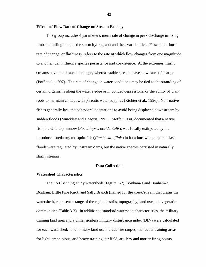
42
Effects of Flow Rate of Change on Stream Ecology
This group includes 4 parameters, mean rate of change in peak discharge in rising
limb and falling limb of the storm hydrograph and their variabilities. Flow conditions’
rate of change, or flashiness, refers to the rate at which flow changes from one magnitude
to another, can influence species persistence and coexistence. At the extremes, flashy
streams have rapid rates of change, whereas stable streams have slow rates of change
(Poff et al., 1997). The rate of change in water conditions may be tied to the stranding of
certain organisms along the water's edge or in ponded depressions, or the ability of plant
roots to maintain contact with phreatic water supplies (Richter et al., 1996). Non-native
fishes generally lack the behavioral adaptations to avoid being displaced downstream by
sudden floods (Minckley and Deacon, 1991). Meffe (1984) documented that a native
fish, the Gila topminnow (Poeciliopsis occidentalis), was locally extirpated by the
introduced predatory mosquitofish (Gambusia affinis) in locations where natural flash
floods were regulated by upstream dams, but the native species persisted in naturally
flashy streams.
Data Collection
Watershed Characteristics
The Fort Benning study watersheds (Figure 3-2), Bonham-1 and Bonham-2,
Bonham, Little Pine Knot, and Sally Branch (named for the creek/stream that drains the
watershed), represent a range of the region’s soils, topography, land use, and vegetation
communities (Table 3-2). In addition to standard watershed characteristics, the military
training land area and a dimensionless military disturbance index (DIN) were calculated
for each watershed. The military land use include fire ranges, maneuver training areas
for light, amphibious, and heavy training, air field, artillery and mortar firing points,
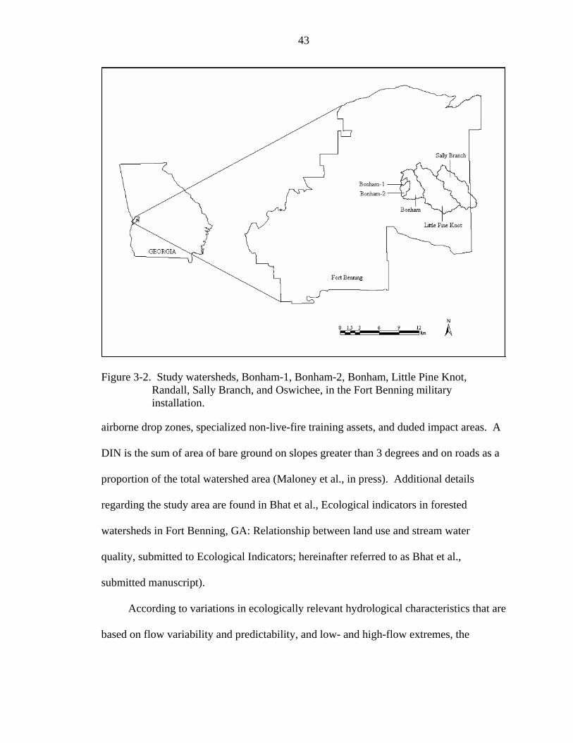
43
Figure 3-2. Study watersheds, Bonham-1, Bonham-2, Bonham, Little Pine Knot,
Randall, Sally Branch, and Oswichee, in the Fort Benning military installation.
airborne drop zones, specialized non-live-fire training assets, and duded impact areas. A
DIN is the sum of area of bare ground on slopes greater than 3 degrees and on roads as a
proportion of the total watershed area (Maloney et al., in press). Additional details
regarding the study area are found in Bhat et al., Ecological indicators in forested
watersheds in Fort Benning, GA: Relationship between land use and stream water
quality, submitted to Ecological Indicators; hereinafter referred to as Bhat et al.,
submitted manuscript).
According to variations in ecologically relevant hydrological characteristics that are
based on flow variability and predictability, and low- and high-flow extremes, the
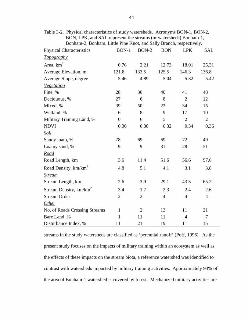
44
Table 3-2. Physical characteristics of study watersheds. Acronyms BON-1, BON-2, BON, LPK, and SAL represent the streams (or watersheds) Bonham-1, Bonham-2, Bonham, Little Pine Knot, and Sally Branch, respectively.
Physical Characteristics BON-1 BON-2 BON LPK SAL Topography
Area, km2 0.76 2.21 12.73 18.01 25.31 Average Elevation, m 121.8 133.5 125.5 146.3 136.8 Average Slope, degree 5.46 4.89 5.04 5.32 5.42 Vegetation Pine, % 28 30 40 41 48 Deciduous, % 27 6 8 2 12 Mixed, % 39 50 22 34 15 Wetland, % 6 8 9 17 10 Military Training Land, % 0 6 5 2 2 NDVI 0.36 0.30 0.32 0.34 0.36 Soil Sandy loam, % 78 69 69 72 49 Loamy sand, % 9 9 31 28 51 Road Road Length, km 3.6 11.4 51.6 56.6 97.6
Road Density, km/km2 4.8 5.1 4.1 3.1 3.8 Stream Stream Length, km 2.6 3.9 29.1 43.3 65.2
Stream Density, km/km2 3.4 1.7 2.3 2.4 2.6 Stream Order 2 2 4 4 4 Other No. of Roads Crossing Streams 1 2 13 11 21 Bare Land, % 1 11 11 4 7 Disturbance Index, % 11 21 19 11 15 streams in the study watersheds are classified as ‘perennial runoff’ (Poff, 1996). As the
present study focuses on the impacts of military training within an ecosystem as well as
the effects of these impacts on the stream biota, a reference watershed was identified to
contrast with watersheds impacted by military training activities. Approximately 94% of
the area of Bonham-1 watershed is covered by forest. Mechanized military activities are
45
not conducted in this watershed as compared to 2-6% of the total area of other watersheds
used for the same purpose. Also, the watershed has a small percentage of bare land,
limited roads, and only one road crossing the stream. Hence, Bonham-1 was used as a
reference watershed for this study.
Precipitation and Streamflow Data
Streamflow and precipitation were measured from January 2000 to December
2003. Precipitation was measured by twelve tipping bucket rain gauges distributed
throughout the study area. Watershed precipitation was determined by areal weighting
using the Thiessen polygon method. Daily discharge values for Bonham-1 and Bonham-
2 were calculated from ten-minute continuous stage records using rating curves. Stream
stage and velocity were measured half-hourly for Bonham, Little Pine Knot, and Sally
Branch. These data were used to calculate daily discharges using the area-velocity
method.
Methods
Annual-Based Hydrologic Indices
The annual-based approach uses multi-year streamflow records to define a series of
ecologically relevant hydrologic indices. These indices may be used to characterize
intra-annual variation in water conditions, analyze temporal variations, and compare
impacts of alteration among watersheds. For this assessment, nonredundant yet
biologically significant hydrologic indices are adapted as per the recommendations of
Olden and Poff (2003). Table 3-3 lists these indices for the perennial runoff type of
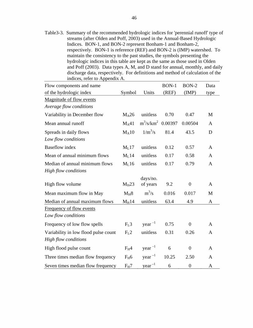
46
Table3-3. Summary of the recommended hydrologic indices for 'perennial runoff' type of streams (after Olden and Poff, 2003) used in the Annual-Based Hydrologic Indices. BON-1, and BON-2 represent Bonham-1 and Bonham-2, respectively. BON-1 is reference (REF) and BON-2 is (IMP) watershed. To maintain the consistency to the past studies, the symbols presenting the hydrologic indices in this table are kept as the same as those used in Olden and Poff (2003). Data types A, M, and D stand for annual, monthly, and daily discharge data, respectively. For definitions and method of calculation of the indices, refer to Appendix A.
Flow components and name BON-1 BON-2 Data of the hydrologic index Symbol Units (REF) (IMP) type Magnitude of flow events Average flow conditions
Variability in December flow MA26 unitless 0.70 0.47 M
Mean annual runoff MA41 m3/s/km2 0.00397 0.00504 A
Spreads in daily flows MA10 1/m3/s 81.4 43.5 D Low flow conditions
Baseflow index ML17 unitless 0.12 0.57 A
Mean of annual minimum flows ML14 unitless 0.17 0.58 A
Median of annual minimum flows ML16 unitless 0.17 0.79 A High flow conditions
High flow volume MH23 days/no. of years 9.2 0 A
Mean maximum flow in May MH8 m3/s 0.016 0.017 M
Median of annual maximum flows MH14 unitless 63.4 4.9 A Frequency of flow events Low flow conditions
Frequency of low flow spells FL3 year –1 0.75 0 A
Variability in low flood pulse count FL2 unitless 0.31 0.26 A High flow conditions
High flood pulse count FH4 year –1 6 0 A
Three times median flow frequency FH6 year –1 10.25 2.50 A
Seven times median flow frequency FH7 year –1 6 0 A
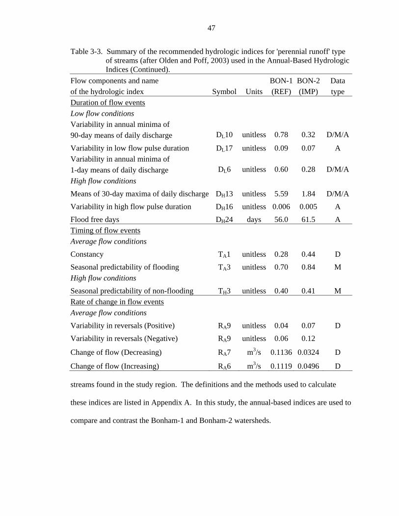
47
Table 3-3. Summary of the recommended hydrologic indices for 'perennial runoff' type of streams (after Olden and Poff, 2003) used in the Annual-Based Hydrologic Indices (Continued).
Flow components and name BON-1 BON-2 Data of the hydrologic index Symbol Units (REF) (IMP) type Duration of flow events Low flow conditions Variability in annual minima of 90-day means of daily discharge DL10 unitless 0.78 0.32 D/M/A
Variability in low flow pulse duration DL17 unitless 0.09 0.07 A Variability in annual minima of 1-day means of daily discharge DL6 unitless 0.60 0.28 D/M/AHigh flow conditions
Means of 30-day maxima of daily discharge DH13 unitless 5.59 1.84 D/M/A
Variability in high flow pulse duration DH16 unitless 0.006 0.005 A
Flood free days DH24 days 56.0 61.5 A Timing of flow events Average flow conditions
Constancy TA1 unitless 0.28 0.44 D
Seasonal predictability of flooding TA3 unitless 0.70 0.84 M High flow conditions
Seasonal predictability of non-flooding TH3 unitless 0.40 0.41 M Rate of change in flow events Average flow conditions
Variability in reversals (Positive) RA9 unitless 0.04 0.07 D
Variability in reversals (Negative) RA9 unitless 0.06 0.12
Change of flow (Decreasing) RA7 m3/s 0.1136 0.0324 D
Change of flow (Increasing) RA6 m3/s 0.1119 0.0496 D streams found in the study region. The definitions and the methods used to calculate
these indices are listed in Appendix A. In this study, the annual-based indices are used to
compare and contrast the Bonham-1 and Bonham-2 watersheds.
48
Storm-Based Hydrologic Indices
The storm-based approach uses the storm hydrographs to determine the indices.
Hydrograph separation was used to identify distinct storm events. 44-100 storm events
from 2001 to 2003 were used to calculate the response factor, baseflow index,
dimensionless indices (Trl/Tlc, Tr/Tlc, and Tb/Tlc), watershed area (A) scaled peak
discharge (qpk/A), bankfull discharges, and the rate of change of peak discharges in rising
and falling limbs for five watersheds, where Bonham-1 is the reference watershed (Table
3-4). Appendix B lists the indices, definitions, and the methods of calculation.
Statistical Analyses
The ANOVA and the Tukey’s multiple comparison tests were performed to
determine the differences between reference watershed and the impacted watersheds’
mean values of indices. The percent of forest extent, military training land, road density,
the number of roads crossing streams, bare land fraction, and disturbance index were
considered to assess the effects of disturbance on hydrology and the potential impact on
stream ecology. Pearson’s correlation coefficients were calculated to examine the
strength and significance of the relationships between a watershed physical characteristic
and storm-based hydrologic index. Stepwise multiple linear regressions were performed
to identify relationships between an index and management related watershed
characteristics. Only variables having p-values less than or equal to 0.05 were retained in
the regression models.
Results
Watershed Disturbance Characteristics
The watersheds’ physical characteristics are summarized in Table 3-2. Most of the
watersheds are highly vegetated (70% or more) with the majority characterized by pine
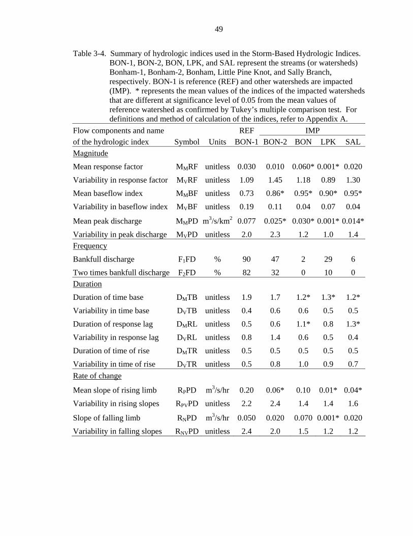
49
Table 3-4. Summary of hydrologic indices used in the Storm-Based Hydrologic Indices. BON-1, BON-2, BON, LPK, and SAL represent the streams (or watersheds) Bonham-1, Bonham-2, Bonham, Little Pine Knot, and Sally Branch, respectively. BON-1 is reference (REF) and other watersheds are impacted (IMP). * represents the mean values of the indices of the impacted watersheds that are different at significance level of 0.05 from the mean values of reference watershed as confirmed by Tukey’s multiple comparison test. For definitions and method of calculation of the indices, refer to Appendix A.
Flow components and name REF IMP of the hydrologic index Symbol Units BON-1 BON-2 BON LPK SAL Magnitude
Mean response factor MMRF unitless 0.030 0.010 0.060* 0.001* 0.020
Variability in response factor MVRF unitless 1.09 1.45 1.18 0.89 1.30
Mean baseflow index MMBF unitless 0.73 0.86* 0.95* 0.90* 0.95*
Variability in baseflow index MVBF unitless 0.19 0.11 0.04 0.07 0.04
Mean peak discharge MMPD m3/s/km2 0.077 0.025* 0.030* 0.001* 0.014*
Variability in peak discharge MVPD unitless 2.0 2.3 1.2 1.0 1.4 Frequency
Bankfull discharge F1FD % 90 47 2 29 6
Two times bankfull discharge F2FD % 82 32 0 10 0 Duration
Duration of time base DMTB unitless 1.9 1.7 1.2* 1.3* 1.2*
Variability in time base DVTB unitless 0.4 0.6 0.6 0.5 0.5
Duration of response lag DMRL unitless 0.5 0.6 1.1* 0.8 1.3*
Variability in response lag DVRL unitless 0.8 1.4 0.6 0.5 0.4
Duration of time of rise DMTR unitless 0.5 0.5 0.5 0.5 0.5
Variability in time of rise DVTR unitless 0.5 0.8 1.0 0.9 0.7 Rate of change
Mean slope of rising limb RPPD m3/s/hr 0.20 0.06* 0.10 0.01* 0.04*
Variability in rising slopes RPVPD unitless 2.2 2.4 1.4 1.4 1.6
Slope of falling limb RNPD m3/s/hr 0.050 0.020 0.070 0.001* 0.020
Variability in falling slopes RNVPD unitless 2.4 2.0 1.5 1.2 1.2
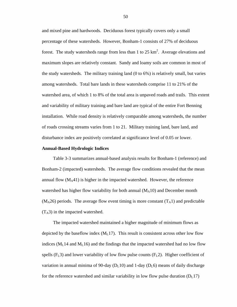
50
and mixed pine and hardwoods. Deciduous forest typically covers only a small
percentage of these watersheds. However, Bonham-1 consists of 27% of deciduous
forest. The study watersheds range from less than 1 to 25 km2. Average elevations and
maximum slopes are relatively constant. Sandy and loamy soils are common in most of
the study watersheds. The military training land (0 to 6%) is relatively small, but varies
among watersheds. Total bare lands in these watersheds comprise 11 to 21% of the
watershed area, of which 1 to 8% of the total area is unpaved roads and trails. This extent
and variability of military training and bare land are typical of the entire Fort Benning
installation. While road density is relatively comparable among watersheds, the number
of roads crossing streams varies from 1 to 21. Military training land, bare land, and
disturbance index are positively correlated at significance level of 0.05 or lower.
Annual-Based Hydrologic Indices
Table 3-3 summarizes annual-based analysis results for Bonham-1 (reference) and
Bonham-2 (impacted) watersheds. The average flow conditions revealed that the mean
annual flow (MA41) is higher in the impacted watershed. However, the reference
watershed has higher flow variability for both annual (MA10) and December month
(MA26) periods. The average flow event timing is more constant (TA1) and predictable
(TA3) in the impacted watershed.
The impacted watershed maintained a higher magnitude of minimum flows as
depicted by the baseflow index (ML17). This result is consistent across other low flow
indices (ML14 and ML16) and the findings that the impacted watershed had no low flow
spells (FL3) and lower variability of low flow pulse counts (FL2). Higher coefficient of
variation in annual minima of 90-day (DL10) and 1-day (DL6) means of daily discharge
for the reference watershed and similar variability in low flow pulse duration (DL17)
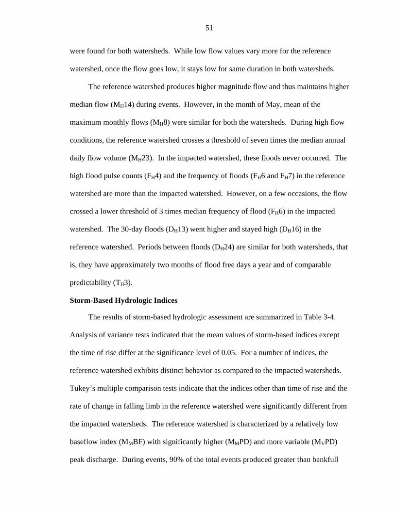
51
were found for both watersheds. While low flow values vary more for the reference
watershed, once the flow goes low, it stays low for same duration in both watersheds.
The reference watershed produces higher magnitude flow and thus maintains higher
median flow (MH14) during events. However, in the month of May, mean of the
maximum monthly flows (MH8) were similar for both the watersheds. During high flow
conditions, the reference watershed crosses a threshold of seven times the median annual
daily flow volume (MH23). In the impacted watershed, these floods never occurred. The
high flood pulse counts (FH4) and the frequency of floods (FH6 and FH7) in the reference
watershed are more than the impacted watershed. However, on a few occasions, the flow
crossed a lower threshold of 3 times median frequency of flood (FH6) in the impacted
watershed. The 30-day floods (DH13) went higher and stayed high (DH16) in the
reference watershed. Periods between floods (DH24) are similar for both watersheds, that
is, they have approximately two months of flood free days a year and of comparable
predictability (TH3).
Storm-Based Hydrologic Indices
The results of storm-based hydrologic assessment are summarized in Table 3-4.
Analysis of variance tests indicated that the mean values of storm-based indices except
the time of rise differ at the significance level of 0.05. For a number of indices, the
reference watershed exhibits distinct behavior as compared to the impacted watersheds.
Tukey’s multiple comparison tests indicate that the indices other than time of rise and the
rate of change in falling limb in the reference watershed were significantly different from
the impacted watersheds. The reference watershed is characterized by a relatively low
baseflow index (MMBF) with significantly higher (MMPD) and more variable (MVPD)
peak discharge. During events, 90% of the total events produced greater than bankfull

52
discharge (F1FD) in the reference watershed indicating a highly connected system as
compared to 2-47% in impacted watersheds.
Storm flows consistently lasted longer and responded faster to rain events in the
reference watershed (DMTB and DVTB). Once the stream responded, the time of rise
(MMTR) was similar in all the watersheds. The reference watershed’s combination of
fast response and high peak discharge results in a rapidly increasing rising limb (RPPD)
as compared to impacted watersheds.
Relationship between Military Land Management and Storm-Based Hydrologic Indices
Correlation and regression analyses were performed to determine the relationship
among the watershed physical characteristics and the storm-based hydrologic indices.
Table 3-5 indicates that 7 key storm-based hydrologic indices are significantly related to
military land management. Increased military training land, bare land, and the
disturbance index will increase the time of rise as well as the variability in the time base.
Increasing the road density increases the variability in the time base and the rate of
change of rising limb. Increasing the number of roads crossing streams increases the
storm response lag, but decreases the time base. Results also show that an increase in the
number of roads crossing streams decreases the variability in the rate of change of falling
limb. No effects on hydrologic indices were identified for forestry management
practices.
Stepwise multiple correlations characterized the response of storm-based indices to
military impacts (Table 3-6). The greatest impact of land management is found with
statistically significant predictive models for indices of time base, response lag, and time
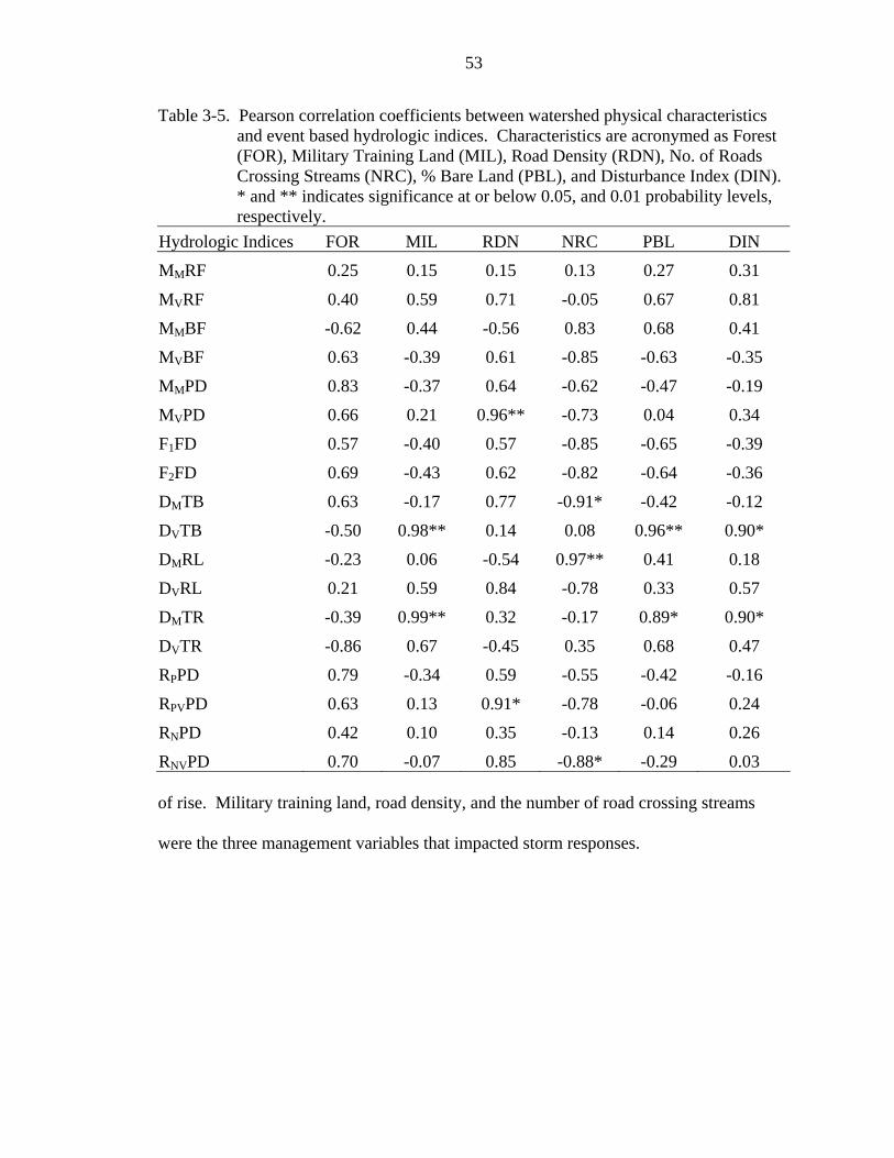
53
Table 3-5. Pearson correlation coefficients between watershed physical characteristics and event based hydrologic indices. Characteristics are acronymed as Forest (FOR), Military Training Land (MIL), Road Density (RDN), No. of Roads Crossing Streams (NRC), % Bare Land (PBL), and Disturbance Index (DIN). * and ** indicates significance at or below 0.05, and 0.01 probability levels, respectively.
Hydrologic Indices FOR MIL RDN NRC PBL DIN
MMRF 0.25 0.15 0.15 0.13 0.27 0.31
MVRF 0.40 0.59 0.71 -0.05 0.67 0.81
MMBF -0.62 0.44 -0.56 0.83 0.68 0.41
MVBF 0.63 -0.39 0.61 -0.85 -0.63 -0.35
MMPD 0.83 -0.37 0.64 -0.62 -0.47 -0.19
MVPD 0.66 0.21 0.96** -0.73 0.04 0.34
F1FD 0.57 -0.40 0.57 -0.85 -0.65 -0.39
F2FD 0.69 -0.43 0.62 -0.82 -0.64 -0.36
DMTB 0.63 -0.17 0.77 -0.91* -0.42 -0.12
DVTB -0.50 0.98** 0.14 0.08 0.96** 0.90*
DMRL -0.23 0.06 -0.54 0.97** 0.41 0.18
DVRL 0.21 0.59 0.84 -0.78 0.33 0.57
DMTR -0.39 0.99** 0.32 -0.17 0.89* 0.90*
DVTR -0.86 0.67 -0.45 0.35 0.68 0.47
RPPD 0.79 -0.34 0.59 -0.55 -0.42 -0.16
RPVPD 0.63 0.13 0.91* -0.78 -0.06 0.24
RNPD 0.42 0.10 0.35 -0.13 0.14 0.26
RNVPD 0.70 -0.07 0.85 -0.88* -0.29 0.03 of rise. Military training land, road density, and the number of road crossing streams
were the three management variables that impacted storm responses.
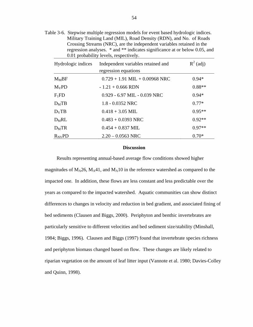
54
Table 3-6. Stepwise multiple regression models for event based hydrologic indices. Military Training Land (MIL), Road Density (RDN), and No. of Roads Crossing Streams (NRC), are the independent variables retained in the regression analyses. * and ** indicates significance at or below 0.05, and 0.01 probability levels, respectively.
Hydrologic indices Independent variables retained and R2 (adj) regression equations
MMBF 0.729 + 1.91 MIL + 0.00968 NRC 0.94*
MVPD - 1.21 + 0.666 RDN 0.88**
F1FD 0.929 - 6.97 MIL - 0.039 NRC 0.94*
DMTB 1.8 - 0.0352 NRC 0.77*
DVTB 0.418 + 3.05 MIL 0.95**
DMRL 0.483 + 0.0393 NRC 0.92**
DMTR 0.454 + 0.837 MIL 0.97**
RNVPD 2.20 – 0.0563 NRC 0.70*
Discussion
Results representing annual-based average flow conditions showed higher
magnitudes of MA26, MA41, and MA10 in the reference watershed as compared to the
impacted one. In addition, these flows are less constant and less predictable over the
years as compared to the impacted watershed. Aquatic communities can show distinct
differences to changes in velocity and reduction in bed gradient, and associated fining of
bed sediments (Clausen and Biggs, 2000). Periphyton and benthic invertebrates are
particularly sensitive to different velocities and bed sediment size/stability (Minshall,
1984; Biggs, 1996). Clausen and Biggs (1997) found that invertebrate species richness
and periphyton biomass changed based on flow. These changes are likely related to
riparian vegetation on the amount of leaf litter input (Vannote et al. 1980; Davies-Colley
and Quinn, 1998).
55
The higher magnitude of the annual-based low flow indices (ML17, ML14, and
ML16) in the impacted watershed is attributed to higher groundwater input as compared
to the reference watershed. This increased input likely reflects the reduction of
interception characteristic of the military land uses (Bryant et al., in press). The relative
magnitude of low flows is likely to have important influences on biota through the
intensity of habitat destruction associated with drying during low flows. In this study, the
lower magnitudes of low flows as depicted by lower baseflow index (ML17) and smaller
low flow pulses (FL3) suggest that the long periods of low flow condition are more likely
in the reference watershed. Higher variability in the duration during low flow condition
(DL10, DL17, and DL6) in the reference watershed supports likelihood of such long
periods of low flow conditions. Long periods of low flow conditions and higher
variability in these conditions may provide selective pressure for specific life history
characteristics such as invertibrate aestivation and egg diapause, and physiological
tolerance to low dissolved oxygen (Williams and Hynes, 1977).
The higher magnitude of the annual-based high flow indices (MH23 and MH14) and
peak discharges (MMPD and MVPD) in the reference watershed as compared to the
impacted watershed suggests the likelihood of habitat regeneration associated with
sediment transport and floodplain inundation during high flows. For high flow events,
the degree of riverbed communities’ disturbance is strongly related to degree of bed
movement (e.g., Biggs et al., 1999). Dissolved inorganic nitrogen and phosphorus
concentrations in rivers are strongly negatively correlated with specific yield and high
flow magnitude among watersheds, and among years within watersheds (e.g., Biggs and
Close, 1989; Close and Davies-Colley, 1990; Grimm and Fisher, 1992). This reflects the
56
degree of flushing of the nutrients mineralized through organic matter breakdown in the
soil profile and leachate from the underlying substrata.
Floods or high flow conditions are also important in influencing community
structure. The results based on the annual flow in this study clearly show that the
reference watershed produced more frequent high flows (FH4, FH6, and FH7). Similarly,
the results from storm-based analysis show that the frequency of discharges equaling or
exceeding bankfull (F1FD and F2FD) is higher in the reference watershed. Floods are
widely viewed as reset mechanisms (Resh et al., 1988), and flood-related mortality to
lotic organisms can result either directly from scouring, crushing, or downstream export
of individuals (Minckley and Maffe, 1987) or indirectly from food resources loss
(Hanson and Waters, 1974). As flood frequency increases, some invertebrates in the
reference watershed actively migrate either into the substratum or to quieter backwaters
to avoid sudden floods. Floods have been shown to regulate community structure by
facilitating local coexistence between asymmetrically competitive algal species (Power
and Stewart, 1987) and invertibrate species (Hemphill and Cooper, 1983) and between an
exotic fish predator and its native, relatively flood-resistant prey (Meffe, 1984). The
result in this study showed the consistency of storm-based F1FD and F2FD with annual-
based FH4, FH6, and FH7 indices suggesting F1FD and F2FD may be used as alternative
indices.
As indicated by the higher annual-based mean duration of high flow condition
(DH13) and the duration of storms (DMTB) in the reference as compared to the impacted
watershed, it is apparent that water resides in the reference watershed for a longer period
of time during high flow condition. However, the DMRL is smaller for the reference
57
watershed suggesting a quick rise in hydrograph. This can be attributed to a better
connectivity of riparian areas to the stream. This connectivity is important as the nutrient
concentrations can strongly control autotrophic production during inter-flood periods
(e.g., Biggs, 2000). Also, individual high flow events greatly reduce the biomass and
change the species composition of periphyton (e.g., Biggs and Stokseth, 1996), and
invertebrates (e.g., Cobb et al., 1992).
Predictive relationships were identified for storm-based hydrologic indices based
on watershed scale military management and suggest that the key variables related to
hydrologic alteration are military training land, road density, and the number of roads
crossing streams. Military training within a watershed can modify annual and storm
generated runoff due to changes in drainage, vegetation, and soils. The impact is due to
troop maneuvers and large, tracked and wheeled vehicles that traverse thousands of
hectares in a single training exercise (Quist et al., 2003). These activities’ impacts,
ranging from minor soil compaction and lodging of standing vegetation to severe
compaction and complete loss of vegetation cover in areas with concentrated training use
(Wilson, 1988; Milchunas et al., 1999), are evident in the stream hydrographs and
suggest impacts to stream ecosystems. Disruption in soil density and water content
(Helvey and Kochenderfer, 1990), addition of sediment, nutrients, and contaminants in
aquatic ecosystems (Gjessing et al., 1984), and impairment of natural habitat
development and woody debris dynamics in forested floodplain streams (Piegay and
Landon, 1997) are potential impacts on terrestrial and aquatic ecosystems. In a recent
study in the same watersheds in Fort Benning, Houser et al. (2004) found that gross
primary productivity, respiration, and the benthic organic matter were low in the stream
58
corresponding to the impacted watershed (higher disturbance index) as compared to the
reference one (lower disturbance index). Road crossings commonly found in military
training areas may act as barriers to the movement of fishes and other aquatic animals
(Furniss et al., 1991). Roads also directly change the hydrology by intercepting shallow
groundwater flow paths, diverting the water along the roadway and routing it efficiently
to streams at crossings (Wemple et al, 1996). This can cause or contribute to changes in
timing and routing of runoff (Jones and Grant, 1996).
Conclusion and Recommendations
In the present study, a reference watershed was compared to impacted watersheds
using annual and storm-based hydrologic indices within the Fort Benning military
installation. The results suggest a subset of the hydrologic indices recommended by
Olden and Poff (2003) are necessary for the Fort Benning streams. It is recommended
that mean annual runoff and its spread, baseflow index, high flow volume, frequency of
low flow spells, high flood pulse count, variability in annual minima of 90-day means of
daily discharges, and constancy be used in stream ecology studies in the Fort Benning
streams to identify disturbances relative to a reference watershed at a watershed scale.
The indices based on storm data may be used to augment the annual indices or as
surrogate to those indices. Storm-based magnitude and variability in peak discharge,
baseflow index, and the bankfull discharge were consistent with the results from annual-
based analysis. With respect to the potential influence of the frequency and duration
aspects of the flow regimes on the stream ecology, duration and variability of time base,
and duration of response lag are identified as critical hydrologic indices. The military
management practices, military training land, road density, and the number of road
crossing streams, were found to significantly affect these indices.
59
CHAPTER 4 PREDICTION OF NITROGEN LEACHING FROM FRESHLY FALLEN LEAVES: APPLICATION OF RIPARIAN ECOSYSTEM MANAGEMENT MODEL (REMM)
Introduction
Forest canopy litterfall initiates the major pathway for recycling of nutrients from
plant to soil (Bubb et al., 1998). Nutrients are returned to the soil via litterfall and
throughfall fluxes in forested ecosystem (Ukonmanaho and Starr, 2001). Litterfall,
comprised predominantly of leaf litter, is usually the most important nutrient source
(Herbohn and Congdon, 1998). Litter quantity, litter decomposition and nutrient release
patterns are factors for understanding nutrient cycling in forest ecosystems (Rogers,
2002). Litterfall is primarily caused by natural senescence of leaves. Forest litterfall
quantity and composition varies among tree species, stand age and development, and
reflects environmental conditions, particularly water and nutrient availability (Binkley,
1986; Polglase and Attiwill, 1992). The amount and distribution of litterfall through time
are also affected by season, rainfall amount and distribution, and wind speed (Crockford
and Richardson, 1998).
Fluxes of dissolved organic matter are an important vector for the movement of
nutrients both within and between ecosystems (Cleveland et al., 2004). In many forest
ecosystems, more than half of the nitrogen is soil solution is in organic form (Qualls et
al., 1991). Hydrology plays an important role in both production and mobilization of
dissolved organic matter in the forest floor (Park and Matzner, 2003). A substantial
amount of potentially soluble organic matter exists in an adsorbed phase (Christ and
60
David, 1996). The amount of percolating water mobilizes these soluble organic matters
(Tipping et al., 1999).
Past studies have shown that the dissolved organic matter flux increases when the
percolating water passes through the forest floor (McDowell and Likens, 1988; Qualls et
al., 1991; Currie et al., 1996; Michalzik et al., 2001). In a recent study in India, Singh et
al. (1999) reported that the rapid mass loss of leaf litter occurred during the rainy season
and the rate of litter mass loss was positively correlated with the cumulative rainfall. In
an early study, Bocock et al. (1960) observed a rapid leaching from oak and ash leaf
litter, and suggested that the weight loss during the first month was largely due to a
physical loss by leaching. The primary sources of dissolved nutrients are considered to
be leaching of substance from fresh litter and the product of decomposition of the plant
litters (Qualls et al., 1991). Water-soluble nutrients are more easily leached from the leaf
litter of deciduous species, including birch, than from coniferous species, including Scots
pine (Pinus sylvestris) and Norway spruce (Picea abies) (Harris and Safford, 1996;
Hongve, 1999).
Depending on the species, leaf litter may release from 5 to 30% of original dry
weight as dissolved organic matter within 24 hours (Cummins, 1974). In a woodland
stream ecosystem in Massachusetts, McDowell and Fisher (1976) found that leaves lose
weight rapidly by abiotic leaching of soluble constituents for 1-3 days and decay more
slowly thereafter as a result of microbial decomposition. Gosz et al. (1973) estimated
15% mass loss for yellow birch leaves (Betula lutea) due to leaching within first month
on the forest floor. Heath et al. (1966) reported a 26% weight loss from birch leaves (B.

61
alba) that remained for two months on the forest floor. Nykvist (1961) found an 8%
weight loss in B. verrucosa after 24 hours of leaching in distilled water.
Annual fluxes of nitrogen in litterfall are greater than other nutrients regardless of
forest type but the amounts vary among forest types (Ukonmaanaho and Starr, 1999).
Dissolved organic nitrogen is the major form of nitrogen in stream water draining from
many mature forest watersheds, comprising about 95% of the total nitrogen (Qualls et al.,
1991). Nitrogen content of a hardwood forest litterfall on the Hubbard Brook
experimental forest comprised approximately 37% of the total nutrients (Gosz et al.,
1972). In a low nutrient system at the Coweeta Hydrologic Laboratory in North Carolina,
where carbon (C) to nitrogen (N) ratios in freshly fallen litter varied from 100 to 220,
Qualls et al. (1991) reported that the output of dissolved organic nitrogen from the forest
floor was 28% of the nitrogen input from the litterfall.
The Riparian Ecosystem Management Model (REMM) was developed by the U.S.
Department of Agriculture’s (USDA) Agricultural Research Service (ARS) to
characterize the role of the riparian area on stream water quality (Lowrance et al., 2000;
Altier et al., 2002). In REMM, the riparian areas’ water quality functions for control of
N, phosphorus (P), and sediment transport into surface waters are simulated and
analyzed. This model has primarily been tested and applied on high-nutrient riparian
buffers adjacent to agricultural fields in the past (e.g., Inamdar et al., 1999a; Inamdar et
al., 1999b; Lowrance et al., 2000).
The complex dynamics related to the nutrients in a watershed is particularly of
interest in low nutrient systems as the release of nutrients from plant litters prior to
decomposition may be an important aspect of characterizing stream water quality. A
62
watershed scale study related to surface water quality was conducted in the Fort Benning
military installation located in southwest Georgia. Experimental data from Fort Benning
shows an increase in total Kjeldahl nitrogen concentrations following litterfall. The
release of nitrogen is relatively rapid as compared to that released from decomposition of
organic matter. It is hypothesized that after leaves fall, the first precipitation events can
be expected to result immediate nitrogen leaching and a corresponding increase in
nitrogen levels in the stream water. The goal of this study is to determine whether freshly
fallen leaves in a riparian area are a significant source of nitrogen in low nutrient system.
The specific objectives of this study are to quantify nitrogen in streamflow using REMM
and verify the modeled results with the observed data.
Basic Concepts of REMM
Originally, REMM was developed to simulate buffer systems that meet
specifications recommended by the USDA Forest Service and the USDA Natural
Resource Conservation Service as a national standard (Natural Resource Conservation
Service, 1995). Three zones parallel to the stream characterize the riparian system. Thus
REMM simulates a three-zone buffer. The riparian area’s soil is characterized in three
layers. In these soil layers, vertical and lateral movement of water and associated
dissolved nutrients takes place. The top two soil layers correspond with the soil horizons
A and B, respectively. Depth of the root zone or a restricting soil horizon defines the
third soil layer. A litter layer that interacts with surface runoff covers the soil layer 1.
The model takes upland water output supplied by the user and calculates loadings of
water, nutrients, sediment, and carbon based on actual area of the zones of a riparian area
(Lowrance et al., 2000).
63
The model input data consist of the physical conditions of the riparian area,
external loadings of water and nutrients to the riparian area, soil, vegetation, and soil
information. Altier et al. (2002) documents a detailed description of the algorithms,
equations, and parameters used in the model.
Hydrology component of REMM
REMM measures water stores and fluxes using a daily water balance. The water
balance includes interception, evapotranspiration, infiltration, vertical drainage, surface
runoff, subsurface lateral flow, upward flux from water table, and deep seepage.
Interception losses occur in the vegetation canopy and litter layer. Canopy interception is
an exponential function of the canopy storage capacity and the amount of daily rainfall,
and is simulated using a modified form of the Thomas and Beasley (1986) equation.
Precipitation falling through the canopy (throughfall) is subject to litter interception.
Similar to canopy interception, litter interception is determined by the mass of the litter at
any given time and the litter storage capacity.
Infiltration at the soil surface depends on the total depth of water. This depth of
water is the sum of the throughfall depth and overland flow depth from the upslope zone
or field. If the sum of incoming upland runoff and throughfall depth is less than the
infiltration capacity of the riparian soil, runoff infiltrates at the rate of application.
During high intensity storms, the runoff and throughfall rate may exceed the infiltration
rate. Surface runoff from the riparian buffer occurs when total water depth exceeds the
infiltration depth. In such conditions, model simulates the infiltration using a modified
form of the Green-Ampt equation (Stone et al., 1994).
When soil moisture exceeds the field capacity, vertical drainage from a soil layer
occurs. This vertical drainage also depends on the available water storage capacity of the
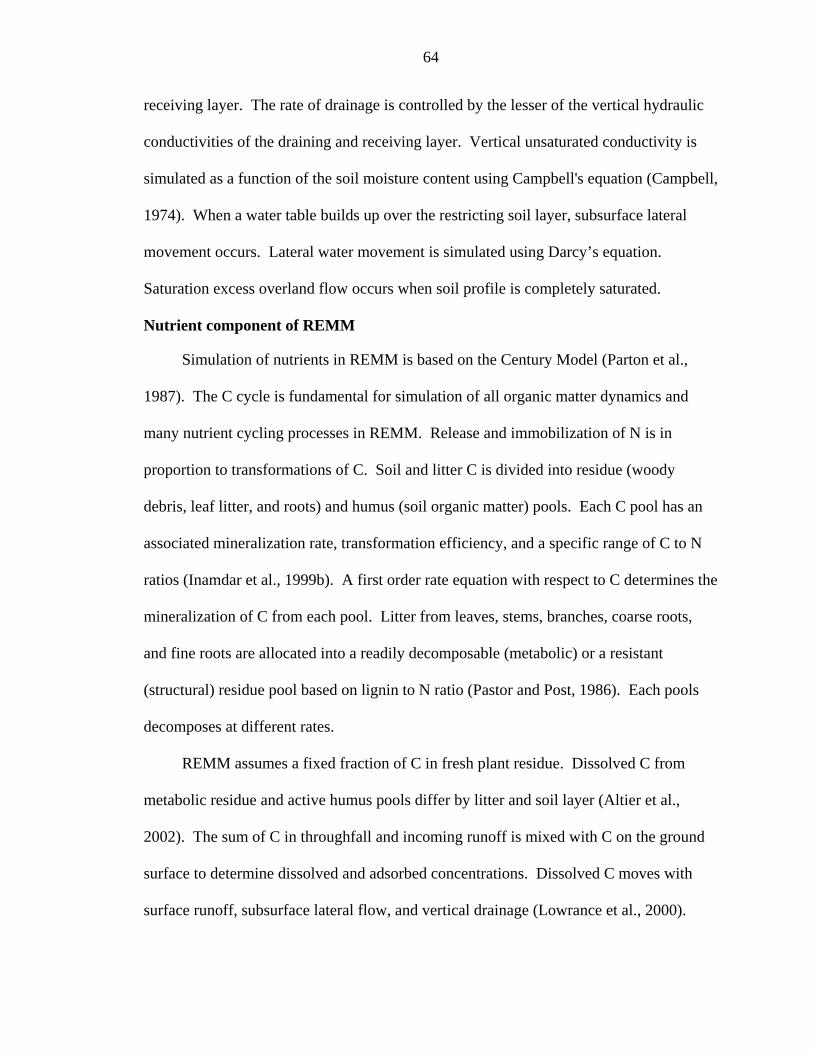
64
receiving layer. The rate of drainage is controlled by the lesser of the vertical hydraulic
conductivities of the draining and receiving layer. Vertical unsaturated conductivity is
simulated as a function of the soil moisture content using Campbell's equation (Campbell,
1974). When a water table builds up over the restricting soil layer, subsurface lateral
movement occurs. Lateral water movement is simulated using Darcy’s equation.
Saturation excess overland flow occurs when soil profile is completely saturated.
Nutrient component of REMM
Simulation of nutrients in REMM is based on the Century Model (Parton et al.,
1987). The C cycle is fundamental for simulation of all organic matter dynamics and
many nutrient cycling processes in REMM. Release and immobilization of N is in
proportion to transformations of C. Soil and litter C is divided into residue (woody
debris, leaf litter, and roots) and humus (soil organic matter) pools. Each C pool has an
associated mineralization rate, transformation efficiency, and a specific range of C to N
ratios (Inamdar et al., 1999b). A first order rate equation with respect to C determines the
mineralization of C from each pool. Litter from leaves, stems, branches, coarse roots,
and fine roots are allocated into a readily decomposable (metabolic) or a resistant
(structural) residue pool based on lignin to N ratio (Pastor and Post, 1986). Each pools
decomposes at different rates.
REMM assumes a fixed fraction of C in fresh plant residue. Dissolved C from
metabolic residue and active humus pools differ by litter and soil layer (Altier et al.,
2002). The sum of C in throughfall and incoming runoff is mixed with C on the ground
surface to determine dissolved and adsorbed concentrations. Dissolved C moves with
surface runoff, subsurface lateral flow, and vertical drainage (Lowrance et al., 2000).
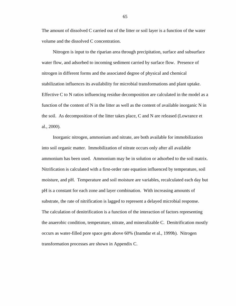
65
The amount of dissolved C carried out of the litter or soil layer is a function of the water
volume and the dissolved C concentration.
Nitrogen is input to the riparian area through precipitation, surface and subsurface
water flow, and adsorbed to incoming sediment carried by surface flow. Presence of
nitrogen in different forms and the associated degree of physical and chemical
stabilization influences its availability for microbial transformations and plant uptake.
Effective C to N ratios influencing residue decomposition are calculated in the model as a
function of the content of N in the litter as well as the content of available inorganic N in
the soil. As decomposition of the litter takes place, C and N are released (Lowrance et
al., 2000).
Inorganic nitrogen, ammonium and nitrate, are both available for immobilization
into soil organic matter. Immobilization of nitrate occurs only after all available
ammonium has been used. Ammonium may be in solution or adsorbed to the soil matrix.
Nitrification is calculated with a first-order rate equation influenced by temperature, soil
moisture, and pH. Temperature and soil moisture are variables, recalculated each day but
pH is a constant for each zone and layer combination. With increasing amounts of
substrate, the rate of nitrification is lagged to represent a delayed microbial response.
The calculation of denitrification is a function of the interaction of factors representing
the anaerobic condition, temperature, nitrate, and mineralizable C. Denitrification mostly
occurs as water-filled pore space gets above 60% (Inamdar et al., 1999b). Nitrogen
transformation processes are shown in Appendix C.

66
Application of REMM
Study Area
The study area consisted of a second-order watershed, Bonham-South (221 ha), in
the Fort Benning military installation, Georgia (Figure 4-1). A detailed description of
this site along with the instrumentation and the type of data collected is provided in
Figure 4-1. Study area. Bonham-South is a second-order watershed within the Fort
Benning military installation in Georgia.
Bryant et al., in press and Bhat et al., in review. The riparian area covers approximately
2.5% of the total watershed area. The riparian length is 3,500 m. Based on the visual
inspection in the watershed, a 12 m wide riparian buffer along the stream is considered.
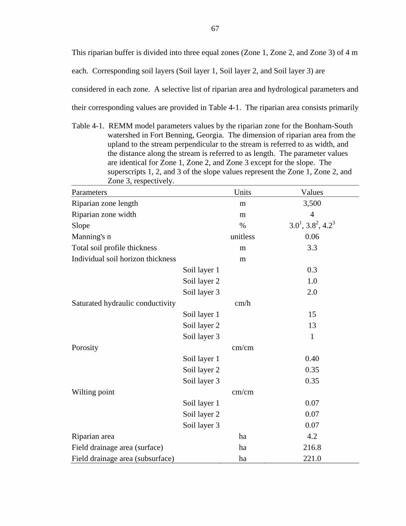
67
This riparian buffer is divided into three equal zones (Zone 1, Zone 2, and Zone 3) of 4 m
each. Corresponding soil layers (Soil layer 1, Soil layer 2, and Soil layer 3) are
considered in each zone. A selective list of riparian area and hydrological parameters and
their corresponding values are provided in Table 4-1. The riparian area consists primarily
Table 4-1. REMM model parameters values by the riparian zone for the Bonham-South watershed in Fort Benning, Georgia. The dimension of riparian area from the upland to the stream perpendicular to the stream is referred to as width, and the distance along the stream is referred to as length. The parameter values are identical for Zone 1, Zone 2, and Zone 3 except for the slope. The superscripts 1, 2, and 3 of the slope values represent the Zone 1, Zone 2, and Zone 3, respectively.
Parameters Units Values Riparian zone length m 3,500 Riparian zone width m 4 Slope % 3.01, 3.82, 4.23 Manning's n unitless 0.06 Total soil profile thickness m 3.3 Individual soil horizon thickness m
Soil layer 1 0.3 Soil layer 2 1.0 Soil layer 3 2.0
Saturated hydraulic conductivity cm/h Soil layer 1 15 Soil layer 2 13 Soil layer 3 1
Porosity cm/cm Soil layer 1 0.40 Soil layer 2 0.35 Soil layer 3 0.35
Wilting point cm/cm Soil layer 1 0.07 Soil layer 2 0.07 Soil layer 3 0.07
Riparian area ha 4.2 Field drainage area (surface) ha 216.8 Field drainage area (subsurface) ha 221.0

68
of hardwoods (approximately 60%) that are mostly scrub oak (Q. rubra), sweetbay (M.
virginiana), sweet gum (L. styraciflua), water oak (Q. nigra), willow oak (Q. phellos),
red maple (A. rubrum), and swamp tupelo (N. aquatica). Mixed species including
southern scrub oak (Q. rubra) and yellow pine (P. ponderosa) cover approximately 21%
of the riparian area, whereas loblolly (P. taeda) and longleaf (P. palustris) pine cover
approximately 19%. The riparian area soils are predominantly sandy loam. The uplands
are mostly on loamy sand.
Data and Input Parameters
REMM operates at a hillslope scale. To apply the model at watershed scale, it is
necessary to convert the watershed into an equivalent hillslope by adjusting the geometry
of watershed. As the riparian buffer has specified length (parallel to the stream) and
width (perpendicular to the stream), upland contributing field width of the watershed was
adjusted to equate the total area of the watershed.
REMM requires soil and vegetation nutrient pools for the riparian area of the
watershed to initialize the model (Table 4-2). Required field data to run the model
includes daily surface and subsurface runoff from the uplands to the riparian area (Table
4-3). The model also requires daily weather data and parameter values representing
topographic, soil, and vegetative conditions within the riparian area. Strategic
Environmental Research and Development Plan’s (SERDP) Ecosystem Management
Project (SEMP) continuously records the atmospheric data within the military
installation. Daily weather data were obtained from SEMP data repository that included
precipitation amount and duration, maximum and minimum air temperatures, solar
radiation, wind speed, and dew point temperature. Daily streamflow for Bonham-South
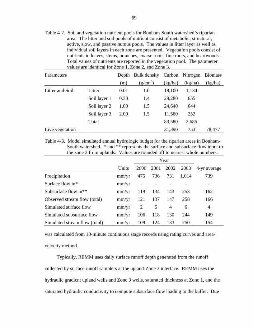
69
Table 4-2. Soil and vegetation nutrient pools for Bonham-South watershed’s riparian area. The litter and soil pools of nutrient consist of metabolic, structural, active, slow, and passive humus pools. The values in litter layer as well as individual soil layers in each zone are presented. Vegetation pools consist of nutrients in leaves, stems, branches, coarse roots, fine roots, and heartwoods. Total values of nutrients are reported in the vegetation pool. The parameter values are identical for Zone 1, Zone 2, and Zone 3.
Parameters Depth Bulk density Carbon Nitrogen Biomass (m) (g/cm3) (kg/ha) (kg/ha) (kg/ha) Litter and Soil Litter 0.01 1.0 18,100 1,134 Soil layer 1 0.30 1.4 29,280 655 Soil layer 2 1.00 1.5 24,640 644 Soil layer 3 2.00 1.5 11,560 252 Total 83,580 2,685 Live vegetation 31,390 753 78,477 Table 4-3. Model simulated annual hydrologic budget for the riparian areas in Bonham-
South watershed. * and ** represents the surface and subsurface flow input to the zone 3 from uplands. Values are rounded off to nearest whole numbers.
Year Units 2000 2001 2002 2003 4-yr averagePrecipitation mm/yr 475 736 731 1,014 739 Surface flow in* mm/yr - - - - - Subsurface flow in** mm/yr 119 134 143 253 162 Observed stream flow (total) mm/yr 121 137 147 258 166 Simulated surface flow mm/yr 2 5 4 6 4 Simulated subsurface flow mm/yr 106 118 130 244 149 Simulated stream flow (total) mm/yr 109 124 133 250 154 was calculated from 10-minute continuous stage records using rating curves and area-
velocity method.
Typically, REMM uses daily surface runoff depth generated from the runoff
collected by surface runoff samplers at the upland-Zone 3 interface. REMM uses the
hydraulic gradient upland wells and Zone 3 wells, saturated thickness at Zone 1, and the
saturated hydraulic conductivity to compute subsurface flow loading to the buffer. Due
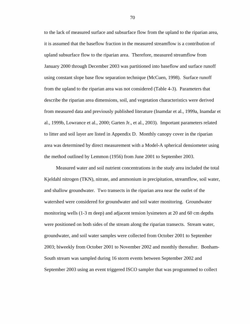
70
to the lack of measured surface and subsurface flow from the upland to the riparian area,
it is assumed that the baseflow fraction in the measured streamflow is a contribution of
upland subsurface flow to the riparian area. Therefore, measured streamflow from
January 2000 through December 2003 was partitioned into baseflow and surface runoff
using constant slope base flow separation technique (McCuen, 1998). Surface runoff
from the upland to the riparian area was not considered (Table 4-3). Parameters that
describe the riparian area dimensions, soil, and vegetation characteristics were derived
from measured data and previously published literature (Inamdar et al., 1999a, Inamdar et
al., 1999b, Lowrance et al., 2000; Garten Jr., et al., 2003). Important parameters related
to litter and soil layer are listed in Appendix D. Monthly canopy cover in the riparian
area was determined by direct measurement with a Model-A spherical densiometer using
the method outlined by Lemmon (1956) from June 2001 to September 2003.
Measured water and soil nutrient concentrations in the study area included the total
Kjeldahl nitrogen (TKN), nitrate, and ammonium in precipitation, streamflow, soil water,
and shallow groundwater. Two transects in the riparian area near the outlet of the
watershed were considered for groundwater and soil water monitoring. Groundwater
monitoring wells (1-3 m deep) and adjacent tension lysimeters at 20 and 60 cm depths
were positioned on both sides of the stream along the riparian transects. Stream water,
groundwater, and soil water samples were collected from October 2001 to September
2003; biweekly from October 2001 to November 2002 and monthly thereafter. Bonham-
South stream was sampled during 16 storm events between September 2002 and
September 2003 using an event triggered ISCO sampler that was programmed to collect

71
hourly samples based on the flow depth. Bhat et al. (unpublished manuscript), describes
the sample analysis procedures for different chemical constituents.
As REMM simulations are performed on a daily time step, and observed TKN
concentrations are of hourly time step, comparisons between the two were based on the
TKN masses produced during the events that lasted 24 hours or longer. The model
simulates the masses of dissolved and particulate organic nitrogen, dissolved ammonium
and nitrate in surface and subsurface flows on a daily basis. The mass of simulated TKN
is the sum of dissolved and particulate organic nitrogen and dissolved ammonium.
Carbon dissolves from metabolic residue and active humus pools. In REMM, incoming
C from precipitation, surface, and subsurface flow is assumed to be in dissolved form.
Carbon available to be dissolved from the active humus pool is a fraction of the total C
present in the same pool. This fraction of set at 0.31 based on an estimate by McGill et al.
(1981) for the proportion of dying bacteria in metabolic form. The total amount of
dissolved C is the sum of metabolic C residue and the dissolved C fraction in the active
humus pool. In REMM, stoichiometric relationships are assumed between C and N in the
organic matter. As C is transformed, corresponding N is also transformed. A Freundlich
isotherm method determines the amount of dissolved ammonium from inorganic pool of
N in REMM. Observed masses of TKN during storm events are calculated by
multiplying the concentrations by the volume of water.
Model Calibration
REMM’s hydrology and nitrogen components were evaluated using data collected
in this study from riparian area as well as data from the literature. Data collected in
nearby watersheds in Fort Benning, Georgia were used to initialize the C and N in the
soil pools (Garten Jr. et al., 2003). The litter C and N pools are based on the literature
72
values (Silveira, M.L., Reddy, K.R. (Department of Soil and Water Science, University
of Florida), Comerford, N.B. (Department of Soil and Water Science, University of
Florida). Litter decomposition and soluble organic carbon and nitrogen release in a
forested ecosystem. Unpublished manuscript). Soil and vegetation nutrient pools for the
riparian area of the watershed are listed in Table 4-2. Bonham-South’s soil layer
thickness, soil porosity, saturated hydraulic conductivity, clay content, carbon decay rate,
and denitrification rate were calibrated.
Model calibration involved the comparison of the simulated streamflow and TKN
output with the measured values. While calibrating hydrology and nutrient components
of the model, parameters such as soil and litter C and N pools, which are based on
literature values, were fixed. Other fixed parameters included riparian length and width,
surface and subsurface draining area. The remaining parameters including soil layer
thickness, saturated hydraulic conductivity, soil porosity, clay content, carbon decay rate,
and denitrification rate in each zone and soil layers of the riparian buffer were adjusted to
match the observed and predicted results.
Fox (1981) recommends mean biased error (MBE) and mean absolute error (MAE)
to measure the difference between observed and model predicted values. Mean biased
error is calculated as the average error between predicted and observed values
accumulated over the total number data points. Mean absolute error considers the
absolute values of the errors. In the present study, MBE and MAE are modified to
calculate the percent difference of modeled streamflow and TKN mass from the observed
values. Mean bias difference (MBD) calculates the average difference accumulated over
the total number of events, expressed as a percent of the observed value. Mean absolute
73
difference (MAD), expressed also as a percent, considers the absolute values of the
differences. Mean absolute difference takes negative values and replaces them with their
absolute values. Observed and modeled streamflow was also compared using the Nash-
Sutcliffe efficiency. The Nash-Sutcliffe efficiency criteria is based on the normalized
least square objective function that evaluates the sum of the squares of flow residuals
(Nash and Sutcliffe, 1970).
Sensitivity Analysis
A sensitivity analysis was performed to determine the effects of key hydrological,
soil, and vegetation parameters on streamflow and TKN fluxes. The parameters were
canopy cover fraction, riparian zone width, soil layer thickness, maximum carbon decay
rate for litter and humus, maximum denitrification rate, soil saturated hydraulic
conductivity, soil porosity, and soil clay content. Each parameter was changed by +10%
and –10% from the values used as the best estimates for the calibration simulations.
Results
Hydrology
Simulated daily flows for the study watershed closely matched the observed flows
(Figure 4-2). Over the 4-year simulation period, MBD and MAD between observed and
predicted streamflow were 2% and 12%, respectively. The model had Nash-Sutcliffe
efficiency of 80%. REMM tends to underestimate the streamflow during low flow and
overestimate during the storms. Approximately 1% of the streamflow was the
contribution from surface runoff generated in the riparian area. Majority of streamflow
output was through the subsurface (Table 4-2).
74
Figure 4-2. Comparison of REMM simulated daily flow with the observed daily flow for
the Bonham-South watershed.
There was considerable variability between and within years for measured
precipitation and streamflow data during study period. It is evident from Figure 4-2 that
an increase in the average flow during the year 2003. This increase was consistent with
the variation in precipitation during the study period. Overall, model simulations for
streamflow can be considered good for the calibrated parameters.
Nitrogen
Observed stream TKN concentrations during the study period showed a strong
correspondence with the leaf fall (Figure 4-3). Approximately 50% of the canopy in the
riparian area dropped during November-January each year. Higher TKN concentrations
were observed during the same period of time. The simulated TKN concentrations also
correspond to simulated leaf fall (Figure 4-4). Modeled TKN concentrations were higher
during high leaf fall months. From October 2001 to December 2003, modeled leaf fall
totaled 12,200 kg/ha, which corresponds to 5,400 kg/ha/yr. As depicted in the figure,
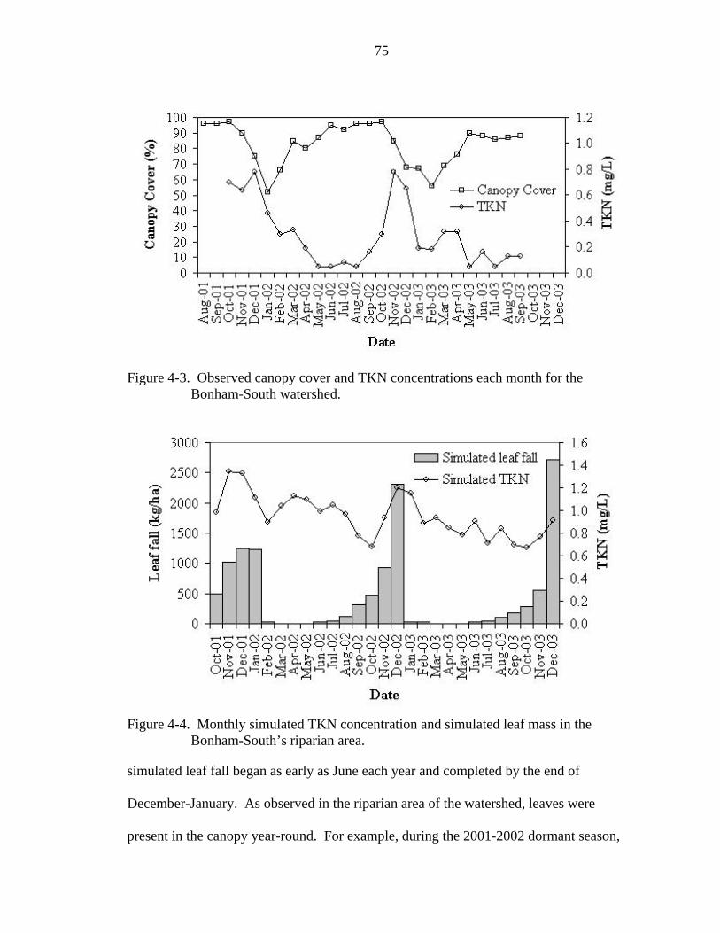
75
Figure 4-3. Observed canopy cover and TKN concentrations each month for the
Bonham-South watershed.
Figure 4-4. Monthly simulated TKN concentration and simulated leaf mass in the
Bonham-South’s riparian area.
simulated leaf fall began as early as June each year and completed by the end of
December-January. As observed in the riparian area of the watershed, leaves were
present in the canopy year-round. For example, during the 2001-2002 dormant season,
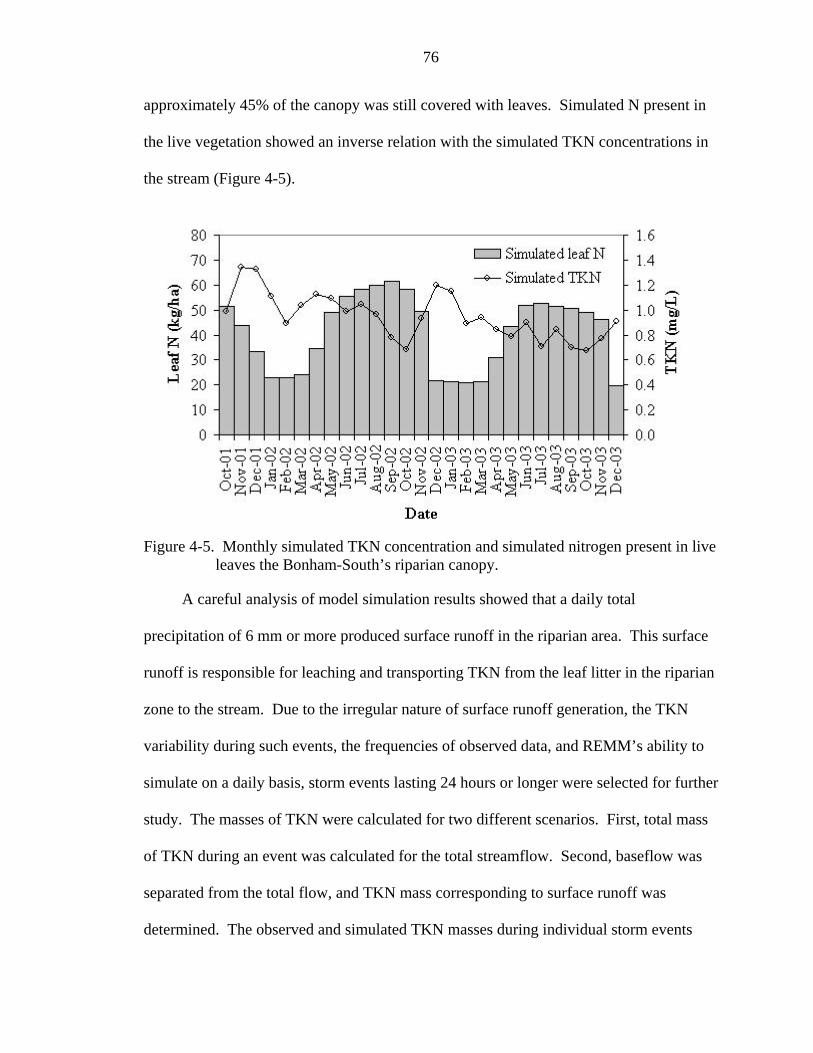
76
approximately 45% of the canopy was still covered with leaves. Simulated N present in
the live vegetation showed an inverse relation with the simulated TKN concentrations in
the stream (Figure 4-5).
Figure 4-5. Monthly simulated TKN concentration and simulated nitrogen present in live
leaves the Bonham-South’s riparian canopy.
A careful analysis of model simulation results showed that a daily total
precipitation of 6 mm or more produced surface runoff in the riparian area. This surface
runoff is responsible for leaching and transporting TKN from the leaf litter in the riparian
zone to the stream. Due to the irregular nature of surface runoff generation, the TKN
variability during such events, the frequencies of observed data, and REMM’s ability to
simulate on a daily basis, storm events lasting 24 hours or longer were selected for further
study. The masses of TKN were calculated for two different scenarios. First, total mass
of TKN during an event was calculated for the total streamflow. Second, baseflow was
separated from the total flow, and TKN mass corresponding to surface runoff was
determined. The observed and simulated TKN masses during individual storm events
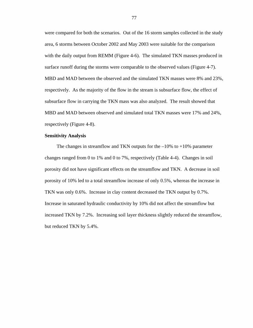
77
were compared for both the scenarios. Out of the 16 storm samples collected in the study
area, 6 storms between October 2002 and May 2003 were suitable for the comparison
with the daily output from REMM (Figure 4-6). The simulated TKN masses produced in
surface runoff during the storms were comparable to the observed values (Figure 4-7).
MBD and MAD between the observed and the simulated TKN masses were 8% and 23%,
respectively. As the majority of the flow in the stream is subsurface flow, the effect of
subsurface flow in carrying the TKN mass was also analyzed. The result showed that
MBD and MAD between observed and simulated total TKN masses were 17% and 24%,
respectively (Figure 4-8).
Sensitivity Analysis
The changes in streamflow and TKN outputs for the –10% to +10% parameter
changes ranged from 0 to 1% and 0 to 7%, respectively (Table 4-4). Changes in soil
porosity did not have significant effects on the streamflow and TKN. A decrease in soil
porosity of 10% led to a total streamflow increase of only 0.5%, whereas the increase in
TKN was only 0.6%. Increase in clay content decreased the TKN output by 0.7%.
Increase in saturated hydraulic conductivity by 10% did not affect the streamflow but
increased TKN by 7.2%. Increasing soil layer thickness slightly reduced the streamflow,
but reduced TKN by 5.4%.
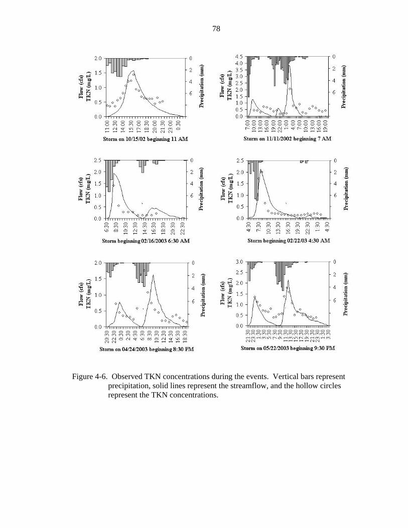
78
Figure 4-6. Observed TKN concentrations during the events. Vertical bars represent
precipitation, solid lines represent the streamflow, and the hollow circles represent the TKN concentrations.
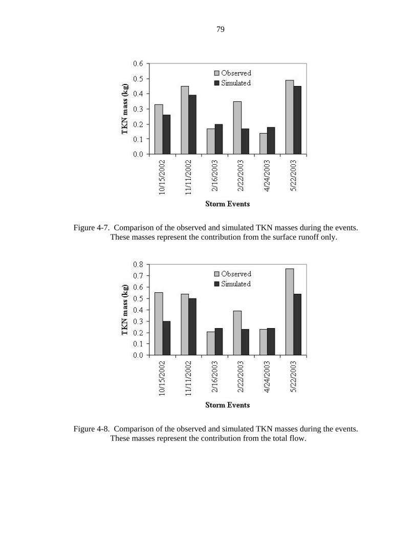
79
Figure 4-7. Comparison of the observed and simulated TKN masses during the events.
These masses represent the contribution from the surface runoff only.
Figure 4-8. Comparison of the observed and simulated TKN masses during the events.
These masses represent the contribution from the total flow.
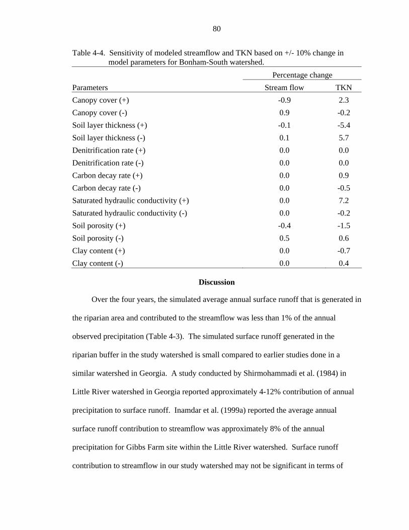
80
Table 4-4. Sensitivity of modeled streamflow and TKN based on +/- 10% change in model parameters for Bonham-South watershed.
Percentage change Parameters Stream flow TKN Canopy cover (+) -0.9 2.3 Canopy cover (-) 0.9 -0.2 Soil layer thickness (+) -0.1 -5.4 Soil layer thickness (-) 0.1 5.7 Denitrification rate (+) 0.0 0.0 Denitrification rate (-) 0.0 0.0 Carbon decay rate (+) 0.0 0.9 Carbon decay rate (-) 0.0 -0.5 Saturated hydraulic conductivity (+) 0.0 7.2 Saturated hydraulic conductivity (-) 0.0 -0.2 Soil porosity (+) -0.4 -1.5 Soil porosity (-) 0.5 0.6 Clay content (+) 0.0 -0.7 Clay content (-) 0.0 0.4
Discussion
Over the four years, the simulated average annual surface runoff that is generated in
the riparian area and contributed to the streamflow was less than 1% of the annual
observed precipitation (Table 4-3). The simulated surface runoff generated in the
riparian buffer in the study watershed is small compared to earlier studies done in a
similar watershed in Georgia. A study conducted by Shirmohammadi et al. (1984) in
Little River watershed in Georgia reported approximately 4-12% contribution of annual
precipitation to surface runoff. Inamdar et al. (1999a) reported the average annual
surface runoff contribution to streamflow was approximately 8% of the annual
precipitation for Gibbs Farm site within the Little River watershed. Surface runoff
contribution to streamflow in our study watershed may not be significant in terms of
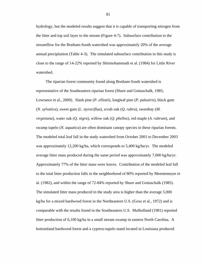
81
hydrology, but the modeled results suggest that it is capable of transporting nitrogen from
the litter and top soil layer to the stream (Figure 4-7). Subsurface contribution to the
streamflow for the Bonham-South watershed was approximately 20% of the average
annual precipitation (Table 4-3). The simulated subsurface contribution in this study is
close to the range of 14-22% reported by Shirmohammadi et al. (1984) for Little River
watershed.
The riparian forest community found along Bonham-South watershed is
representative of the Southeastern riparian forest (Shure and Gottaschalk, 1985;
Lowrance et al., 2000). Slash pine (P. elliotii), longleaf pine (P. palustris), black gum
(N. sylvatica), sweet gum (L. styraciflua), scrub oak (Q. rubra), sweetbay (M.
virginiana), water oak (Q. nigra), willow oak (Q. phellos), red maple (A. rubrum), and
swamp tupelo (N. aquatica) are often dominant canopy species in these riparian forests.
The modeled total leaf fall in the study watershed from October 2001 to December 2003
was approximately 12,200 kg/ha, which corresponds to 5,400 kg/ha/yr. The modeled
average litter mass produced during the same period was approximately 7,000 kg/ha/yr.
Approximately 77% of the litter mass were leaves. Contribution of the modeled leaf fall
to the total litter production falls in the neighborhood of 80% reported by Meentemeyer et
al. (1982), and within the range of 72-84% reported by Shure and Gottaschalk (1985).
The simulated litter mass produced in the study area is higher than the average 5,000
kg/ha for a mixed hardwood forest in the Northeastern U.S. (Gosz et al., 1972) and is
comparable with the results found in the Southeastern U.S. Mulholland (1981) reported
litter production of 6,100 kg/ha in a small stream swamp in eastern North Carolina. A
bottomland hardwood forest and a cypress-tupelo stand located in Louisiana produced

82
litter masses of 5,750 kg/ha and 6,200 kg/ha, respectively (Conner and Day Jr., 1976).
Brinson et al. (1980) reported a value of 6,500 kg/ha for an alluvial swamp forest in
North Carolina.
Simulated results showed that the nitrogen content in the litter during the study
period averaged 77 kg/ha of which approximately 59 kg/ha was the contribution from the
leaves alone. This value is less than 83.4 kg/ha of nitrogen contribution from the
deciduous leaves in the Northeastern U.S. (Gosz et al., 1972). As observed in the riparian
area, 45% canopy was present even during the dormant seasons because of the presence
of approximately 19% of conifers and 21% of mixed species. Modeled results also
support the presence of the carbon in the leaves and the biomass in the canopy. The
modeled result showed that on an average approximately 527 kg/ha of carbon was
present in the canopy during the dormant season. This value of carbon suggests the
presence of approximately 22 kg/ha of nitrogen in the canopy during the same time
(Figure 4-5). Higher concentrations of TKN during the leaf fall and the inverse relation
with the nitrogen present in the canopy support the hypothesis of flushing of nitrogen
from the leaf litter.
The simulated TKN concentrations follow the trend of leaf mass accumulation in
the riparian area suggesting a higher rate of release of TKN from freshly fallen litter
during the fall and early spring. Brinson et al. (1980) reported higher nutrient fluxes
following litterfall in an alluvial swamp forest in North Carolina. In a study of nutrient
content of litterfall in the Southeastern U.S., Gosz et al. (1972) reported that
approximately 56% of the total nutrient was released during September through
December when the majority of litterfall (50%) occurred. A study conducted in cypress
83
swamp forest in Florida, Schlesinger (1978) reported that in the month of November
when 56% litterfall occurred, 45% of nitrogen was released from the system.
Higher TKN concentrations were observed in the Bonham-South stream during the
precipitation events (Figure 4-6). The storm events presented in Figure 4-6 were long
enough to calculate the masses of TKN during the storms to compare REMM’s simulated
daily values. Comparisons of TKN masses produced during the events were comparable
to REMM’s simulated values. The masses of TKN during the storms were calculated for
two different scenarios. When modeled TKN mass contribution of surface runoff that is
produced in the riparian zone was compared with the observed value in the stream, MBD
and MAD for the six storms were 8% and 23%, respectively. Mean biased difference
value is less reliable as there is the risk that large outliers cancel each other out. As MAD
takes negative values and replaces them with their absolute values, large outliers are de-
emphasized; hence it is less sensitive to extreme values. A MAD of 23% in the surface
runoff suggests that the model was able to produce comparable amount of TKN as
observed during the storm. The comparison between observed and simulated TKN mass
from the total flow showed comparable MBD (17%) and MAD (24%). On average, 43%
of the observed total TKN mass was contributed by surface runoff. This result suggests
that the surface runoff during the precipitation events is a major source of leaching
nitrogen from the forest floor and transporting it to the stream.
Conclusion and Recommendations
Originally, REMM was developed to operate at a hillslope scale. The results in this
study suggested that given appropriate upland inputs for a site, REMM can be used at
different scenarios of riparian area width, length of zones, vegetation type, and soil
properties. The trend and magnitude of the observed streamflow for the study watershed
84
was effectively simulated by REMM. The model, however, overestimated the
streamflow during high flow and underestimated during low flow periods. The
hydrologic budget showed a good agreement between observed and predicted
streamflow.
The simulated litter and corresponding leaf masses in the study watershed were
comparable to the values reported in the literature. Due to the model’s longer simulation
time step, a meaningful comparison of simulated and observed TKN was possible only
through the masses produced during storms that were equal to or longer than a day.
Comparison of TKN masses during six different storm events showed similar values both
in the surface runoff and the total flow. The results supported the hypothesis of nitrogen
leaching from freshly fallen leaves during the precipitation events. These results
provided further insight into the nutrient dynamics of the riparian area. The model
simulations respond as expected to precipitation and vegetation patterns over the study
period. Results clearly indicated that the presence of fresh leaf litter in the riparian area
increases the TKN concentration, and hence mass, in the stream. The model effectively
captured the trends of leaf mass accumulation in the riparian area and subsequent high
concentration and mass during those periods. With the present version of REMM, the
comparison between observed and simulated values is possible only on a daily basis.
However, given the fact that the precipitation events and the sampling frequencies are
often shorter, simulation results using a smaller time scale would be useful. Therefore, it
is recommended to modify REMM from its present version of daily time step to a smaller
time step, preferably hourly, for more effective and meaningful interpretation and
evaluation of riparian nutrient flushing.
85
CHAPTER 5 SUMMARY AND CONCLUSION
The National Research Council of the United States has proposed that reliable and
comprehensive environmental indicators be developed to monitor ecological changes
from natural and anthropogenic causes. The military installation in Fort Benning,
Georgia offered a unique opportunity to study military impacts on water quality and
quantity. Ecohydrological approaches were used to relate the effects of anthropogenic
perturbations on water-vegetation-nutrient interactions in the Fort Benning watersheds.
In this research, statistical relationships among water quality parameters and the
watershed physical characteristics in low-nutrient watersheds were identified and
examined. This research also identified and developed hydrologic indices that
characterize the impact of military land management on watershed, and investigated the
riparian corridor’s role on water quality by quantifying the nitrogen leaching from freshly
fallen leaves.
Relationships among watershed physical characteristics and water quality
parameters in the study watersheds and the regression analysis showed that pH, chloride,
total phosphorus, total Kjeldahl nitrogen, total organic carbon, and total suspended solids
are useful indicators of watershed physical characteristics that are susceptible to
perturbations. A comparison of the results between a reference and impacted watershed
in terms of hydrologic indices that are derived from long-term daily flow as well as the
storm-based data showed a clear distinction between the watersheds in terms of
hydrological flow regimes. Storm-based magnitude of baseflow index, magnitude and
86
variability of peak discharge, and the frequency of bankfull discharge were consistent
with the results from annual-based analysis. Results showed that these storm-based
indices might be used as surrogates to the indices derived from long-term data. The
analysis identified the relationships between the extent of military training land, road
density, and the number of roads crossing streams with the storm-based baseflow index,
bankfull discharge, response lag, and time of rise. For the low nutrient systems of this
study, seasonal and storm variations in water quality were found to be strongly influenced
by precipitation events which caused nitrogen leaching from recently fallen leaf litter and
increased nitrogen levels in the stream water.
This study showed that the signatures of military alterations to watershed landscape
are detectable in the water quality and the flow regime. The observed alterations to these
regimes suggest impacts to aquatic ecosystems. The water quality related indicators and
hydrologic indices presented in this research provide specific measures of stream water
quality and instream flow, respectively, that respond to military impacts. Each indicator
is linked to one or more readily measured watershed scale factors. The indicators could
be useful in predicting effects of military land management and evaluating restoration
activities on the quality as well as the quantity of the water.
This research has several implications for the Fort Benning military installation.
The results of this study indicated that baseflow sampling of water quality can be used to
assess the military training impacts on stream water quality. The water quality indicators
identified in this study provide measures of the current watershed conditions. The water
quality indicators identified in this study provide measures of the current watershed
conditions. Changes to stream water quality due to military training within the Fort

87
Benning military installation can be identified by collecting long-term and routine stream
water quality data and comparing indicator values to current conditions. Future activities
should develop indicator thresholds beyond which improved management and restoration
practices should be implemented. As nutrients are one major factor controlling the
quality of the receiving aquatic ecosystems, the thresholds should be based on the
ecosystems impacts.
The U.S. Army manages approximately 4.8×10⁶ hectares of land for military
training, and it has developed the Land Condition Trend Analysis (LCTA) program to
systematically monitor terrestrial impacts from military training and to support the
mitigation and remediation of severely impacted training lands (Quist et al., 2003).
Although the magnitude of the training would differ from one installation to the other, the
nature of the impact remains similar. Military training typically increases soil bulk
densities and compaction, decreases infiltration, diminishes plant growth, degrades water
quality, and affects water quantity. Therefore, the research findings in this study can be
implemented for management and restoration practices to other military installations
across the U.S. to minimize the impacts of the military training. A common finding
between the water quality and quantity signatures is that military training impacts differ
from those found due to agriculture and urbanization. In the former, water quality
degradation impacts typically manifest as high nutrient loads. However, in military
installations, the loss of topsoil and vegetation results in waters that have significantly
lower nutrient levels. In a similar fashion, the hydrologic regimes in watersheds with
significant military impacts suffer from a loss of variability, but exhibit higher annual
discharge values.

88
APPENDIX A ANNUAL-BASED INDICES DEFINITIONS AND CALCULATION PROCEDURES
Symbol Definition Method
MA26 Coefficient of variation in monthly flows for December
Calculate mean monthly flow for December ( diq ), i = 1,…, n; , n = no. of years Calculate mean of all December flows,
DQ−
= nqn
idi /
1∑
=
Calculate standard deviation (SD) of diq
Calculate coefficient of variation, CV = SD/ DQ−
MA41 Mean annual flow divided by watershed area
Calculate mean yearly flow ( yiq ), i = 1,…, n; , n = no. of years Divide yiq by watershed area (A)
Calculate nA
qAQ
n
i
yiy //
1∑
=
−
⎟⎟⎠
⎞⎜⎜⎝
⎛= , i = 1,…, n; , n = no.
of years
MA10 Ranges in daily flows divided by median daily flows (where range in daily flows is the ratio of 20th/80th percentiles in daily flows across all years)
Combine daily flows of all years Calculate 20th percentile ( 20pQ ) Calculate 80th percentile ( 80pQ ) Calculate median flow ( mQ ) Calculate R = 20pQ / 80pQ Calculate R / mQ
ML17 Seven-day minimum flow divided by mean annual daily flows
Calculate mean yearly flow ( yiq ), i = 1,…, n; , n = no. of years Calculate 7-day minimum ( min7q )i flow Calculate ratios Ri = ( min7q )i / yiq
Calculate nRn
ii /
1∑
=

89
ML14 Mean of the lowest annual daily flow divided by median annual daily flow averaged across all years
Extract lowest yearly flow ( min,iq ), i = 1,…, n; , n = no. of years
Calculate nqQn
ii /
1min,min ∑
=
−
=
Calculate median flow ( mQ ) of all years
Calculate mQQ /min
−
ML16 Median of the lowest annual daily flows divided by median annual daily flows averaged across all years
Extract lowest yearly flow ( min,iq ), i = 1,…, n; , n = no. of years
Calculate median ( medQ ) of min,iq Calculate median flow ( mQ ) of all years
Calculate mmed QQ /
MH23 Mean of the high flow volume (calculated as the area between the hydrograph and the upper threshold during the high flow event) divided by median annual daily flow across all years. The upper threshold is defined as 7 times median annual flow
Calculate yearly median flow ( mediq , ), i = 1,…, n; , n = no. of years Calculate 7 times mediq , Calculate the flow volume ( ViQ ) above 7 times
mediq , value
Calculate nQQn
iViV /
1∑
=
−
=
Calculate median flow ( mQ ) of all years
Calculate mV QQ /−
MH8 Mean of the maximum monthly flows for the month of May
Extract maximum flow for May ( miq ), i = 1,…, n; , n = no. of years Calculate mean of all May maximum flows,
MayQ−
= nqn
imi /
1∑
=
MH14 Median of the highest
annual daily flow divided by the median annual daily flow averaged across all years
Calculate median flow ( miQ ),i = 1,…, n; , n = no. of years
Calculate nQQn
imim /
1∑
=
−
=
Extract highest daily flow ( hiQ ) for each year Calculate median of highest daily flow ( medhQ )
Calculate medhQ / mQ−

90
FL3 Total number of low flow spells (threshold equal to 5% of mean daily flow) divided by the record length in years
Combine daily flows of all years Calculate mean daily flow ( meanQ ) Determine the threshold of 0.05* meanQ Determine the numbers of low flow counts below 0.05* meanQ ( lowN ) Calculate lowN / n , n = record length in years
FL2 Coefficient of variation in Fl1, where Fl1 is low flood pulse count, which is the number of annual occurrences during which the magnitude of flow remains below a lower threshold. Hydrologic pulses are defined as those periods within a year in which the flow drops below the 25th percentile (low pulse) of all daily values for the time period
Calculate 25th percentile value for each year ( ipQ 25 ),i = 1,…, n; , n = no. of years Determine the numbers of low flow pulses below 25th percentile for each year ( ilN 25 ) Calculate mean of low flow pulses,
nNNn
iill /
12525 ∑
=
−
=
Calculate standard deviation (SD) of ilN 25
Calculate CV = SD/ 25lN−
FH4 High flood pulse count is the number of annual occurrences during which the magnitude of flow remains above an upper threshold where the upper threshold is defined as 7 times median daily flow, and the value is represented as an average instead of a tabulated count
Calculate yearly median flow ( mediq , ), i = 1,…, n; , n = no. of years Calculate 7 times mediq , Determine the number of high flood pulses above 7 times mediq , ( hiN7 )
Calculate nNNn
ihih /
177 ∑
=
−
=
FH6 Mean number of high flow events per year using an upper threshold of 3 times median flow over all years
Calculate yearly median flow ( mediq , ), i = 1,…, n; , n = no. of years Calculate 3 times mediq , Determine the number of high flood pulses above 3 times mediq , ( hiN3 )
Calculate nNNn
ihih /
133 ∑
=
−
=

91
FH7 Mean number of high flow events per year using an upper threshold of 7 times median flow over all years
Same as FH4
DL10 Coefficient of variation in annual minima of 90-day means of daily discharge
Determine 90-day minimum flow ( iQ min90 ) for each year, i = 1,…, n; , n = no. of years
Calculate nQQn
ii /
1min90min90 ∑
=
−
=
Calculate SD of iQ min90
Calculate CV = min90/−
QSD
DL17 Coefficient of variation in low flow pulse durations
Calculate 25th percentile value for each year ( ipQ 25 ),i = 1,…, n; , n = no. of years Determine duration between low flow pulses below 25th percentile for each year ( ilD 25 ) Calculate mean duration of low flow pulses,
nDDn
iill /
12525 ∑
=
−
=
Calculate standard deviation (SD) of ilD 25
Calculate CV = SD/ 25lD−
DL6 Coefficient of variation in annual minima of 1day means of daily discharge
Determine 1-day minimum flow ( iQ min1 ) for each year, i = 1,…, n; , n = no. of years
Calculate nQQn
ii /
1min1min1 ∑
=
−
=
Calculate SD of iQ min1
Calculate CV = min1/−
QSD
DH13 Mean annual 30-day maximum divided by median flow
Determine 30-day maximum flow ( iQ max30 ) for each year, i = 1,…, n; , n = no. of years
Calculate nQQn
ii /
1max30max30 ∑
=
−
=
Calculate median flow ( miQ ),i = 1,…, n; , n = no. of years

92
Calculate nQQn
imim /
1∑
=
−
=
Determine mQQ−−
/max30
DH16 Coefficient of variation in high flow pulse durations
Calculate 75th percentile value for each year ( ipQ 75 ), i = 1,…, n; , n = no. of years Determine duration between high flow pulses above 75th percentile for each year ( ihD 75 ) Calculate mean duration of high flow pulses,
nDDn
iihh /
17575 ∑
=
−
=
Calculate standard deviation (SD) of ihD 75
Calculate CV = SD/ 75hD−
DH24 Mean annual maximum number of 365 days over all water years during which no floods occurred over all years
Determine flow of magnitude exceeding a return interval of 1.67 years based on log-normal distribution ( yriQ 67.1 ), i = 1,…, n; , n = no. of years Determine the maximum number of 1.67-year flow non-exceedance days each year ( iyrD max67.1 )
Calculate nDDn
iiyryr /
1max67.1
_
max67.1 ∑=
=
TA1 Constancy [Colwell
(1974)] Standardize the daily flow values by median flow, and express as natural logarithm values Divide the log-transformed flow values into 4-6 classes so that these classes cover all the observed flow values Create a matrix of total number of days in a year (columns, t) by number of classes (rows, s) Define the column totals ( jX ), row totals ( iY ), and the grand total (Z) as
∑=
=s
iijj NX
1, ∑
=
=t
jiji NY
1, and
∑∑∑∑ ===i
ij
jj
iji
YXNZ
where Nij is the number of cycles for which the flow is in class i and time j. Determine uncertainty with respect to time
∑=
−=t
j
jj
ZX
ZX
XH1
log)(

93
Determine uncertainty with respect to class
∑=
−=s
i
ii
ZY
ZY
YH1
log)(
Determine uncertainty with respect to the interaction of time and scale
∑∑−=j
ijij
i ZN
ZN
XYH log)(
Determine predictability (P) with the range (0, 1)
sXHXYHP
log)()(1 −
−=
where s is the number of classes Determine the constancy )(C with range (0, 1)
s
YHClog
)(1−=
TA3 Maximum proportion of
all floods over the period of record that fall in any one of six 60-day ‘seasonal’ windows
Determine flow of magnitude exceeding a return interval of 1.67 years based on log-normal distribution ( yrQ 67.1 ) over the period of record Divide every year into six 60-day ‘seasonal’ windows Determine the maximum number of
yrQ 67.1 exceedance days ( max67.1 yrD ) over period of record in any one of six 60-day ‘seasonal’ windows Determine the total number of yrQ 67.1 exceedance days over all years in one of six 60-day seasonal window ( yrtotD 67.1 ) Calculate the ratio ( max67.1 yrD / yrtotD 67.1 )
TH3 Maximum proportion of the year (number of days/365) during which no floods have ever occurred over the period of record
Determine flow of magnitude exceeding a return interval of 1.67 years based on log-normal distribution ( yrQ 67.1 ) over the period of record Determine the maximum number of yrQ 67.1 non-exceedance days ( yrnonD 67.1 ) over period of record Determine the total number of yrQ 67.1 non-exceedance days over period of record ( yrtotD 67.1 ) Calculate the ratio ( yrnonD 67.1 / yrtotD 67.1 )

94
RA9 Coefficient of variation in number of negative and positive changes in water conditions from one day to the next
Determine number of rises from one day to the other each year ( RiN ), i = 1,…, n; , n = no. of years Determine number of falls each year ( FiN )
Calculate nNNn
iRiR /
1∑
=
−
=
Calculate SDR of RiN
Calculate nNNn
iFiF /
1∑
=
−
=
Calculate SDF of FiN
Calculate CVR = SDR /−
RN
Calculate CVF = SDF /−
FN
RA7 Median of difference between natural logarithm of flows between two consecutive days with decreasing flow
Transform the daily flow values for each year using natural logarithm, Qi = ln Qi, i = no. of days For all ln Qs each year, determine [ln Qi – ln Qi+1] Separate the values of decreasing flow differences for each year Determine the median of decreasing flow differences each year ( dmjQ ), j = 1, …, n; n = no. of years
Calculate nQQn
jdmjdm /
1∑
=
−
=
RA6 Median of difference
between natural logarithm of flows between two consecutive days with increasing flow
Transform the daily flow values for each year using natural logarithm, Qi = ln Qi, i = no. of days For all ln Qs each year, determine [ln Qi – ln Qi+1] Separate the values of increasing flow differences for each year Determine the median of increasing flow differences each year ( imjQ ), j = 1, …, n; n = no. of years
Calculate nQQn
jimjim /
1∑
=
−
=

95
APPENDIX B STORM-BASED INDICES DEFINITIONS AND CALCULATION PROCEDURES
Index Symbol
Definition Methods
MMRF Mean value of the response factor
Calculate precipitation depth for each event ( iP ), i = 1,…,n; n = no. of events Create hydrograph Separate baseflow Calculate DRO depth after deducting the baseflow portion from the hydrograph for each event ( iD ) Calculate response factor for each event, iii PDRF /=
Calculate the mean, nRFRFn
ii /
1
_
∑=
=
MVRF
Coefficient of variation in response factors
Calculate _
RF Calculate standard deviation (SD) of RFi
Calculate _
/ RFSDCV =
MMBF
Mean value of baseflow index
Create hydrograph Separate baseflow Determine baseflow volume (Vb) and total volume (Vt) for each events Calculate BFi = (Vb/Vt,)i, i = 1,…,n; n = no. of events
Calculate the mean, nBFBFn
ii /
1
_
∑=
=
MVBF
Coefficient of variation in baseflow index
Calculate _
BF Calculate (SD) of BFi
Calculate _
/ BFSDCV =
MMPD
Mean value of peak discharges divided by the watershed area
Determine (qpk)i of the event, i = 1,…,n; n = no. of events Normalize (qpk)i by the watershed area, Aq ipk /)(
Calculate mean, ( )_/ Aq pk = ∑
=⎟⎟⎠
⎞⎜⎜⎝
⎛n
i i
pk nA
q
1/

96
MVPD
Coefficient of variation in peak discharges
Calculate ( )_/ Aq pk
Calculate (SD) of Aq ipk /)(
Calculate CV = SD / ( )_/ Aq pk
F1FD Percentage of peak
discharge equals bankfull discharge
Determine bankfull discharge Count peak discharges equal to bankfull discharge for all events and express the count as a percentage of total events
F2FD
Percentage of peak discharge 2 times above bankfull discharge
Determine bankfull discharge Count peak discharges equal to 2.0 times bankfull discharge for all events and express the count as a percentage of total events
DMTB
Mean value of time base divided by the watershed response time
Determine time base for each hydrograph Normalize the time base by the response time (Tbi), i = 1,…,n; n = no. of events
Calculate mean, nTTn
ibib /
1
_
∑=
=
DVTB
Coefficient of variation in time base
Calculate _
bT Calculate (SD) of (Tbi)
Calculate CV = SD/_
bT
DMRL
Mean value of response lag divided by the watershed response time
Determine response lag for each hydrograph Normalize the response lag by the response time (Trli), i = 1,…,n; n = no. of events
Calculate mean, nTTn
irlirl /
1
_
∑=
=
DVRL
Coefficient of variation in response lag
Calculate _
rlT Calculate (SD) of (Trli)
Calculate CV = SD/_
rlT
DMTR
Mean value of time of rise divided by the watershed response time
Determine time of rise for each hydrograph Normalize the time of rise by the response time (Tri), i = 1,…,n; n = no. of events
Calculate mean, nTTn
irir /
1
_
∑=
=

97
DVTR
Coefficient of variation in time of rise
Calculate _
rT Calculate (SD) of (Tri)
Calculate CV = SD/_
rT
RPPD
Mean rate of change in peak discharge in rising limb
Determine (qpk)i of the event, i = 1,…,n; n = no. of events Normalize (qpk)i by the watershed area, Aq ipk /)( Normalize the time of rise by the response time (Tri), i = 1,…,n; n = no. of events Calculate the ratio of Aq ipk /)( to (Tri) Calculate the mean of the ratios
RPVPD
Coefficient of variation in the rate of change in peak discharge in rising limb
Calculate mean of RPPDi Calculate (SD) of RPPDi Calculate CV = SD/mean of RPPDi
RNPD
Mean rate of change in peak discharge in falling limb
Determine (qpk)i of the event, i = 1,…,n; n = no. of events Normalize (qpk)i by the watershed area, Aq ipk /)( Normalize the time of rise by the response time (Tri), i = 1,…,n; n = no. of events Normalize the time base by the response time (Tbi) Calculate the difference (Tbi - Tri) Calculate the ratio of Aq ipk /)( to (Tbi - Tri) Calculate the mean of the ratios
RNVPD
Coefficient of variation in the rate of change in peak discharge in falling limb
Calculate mean of RNPDi Calculate (SD) of RNPDi Calculate CV = SD/mean of RNPDi
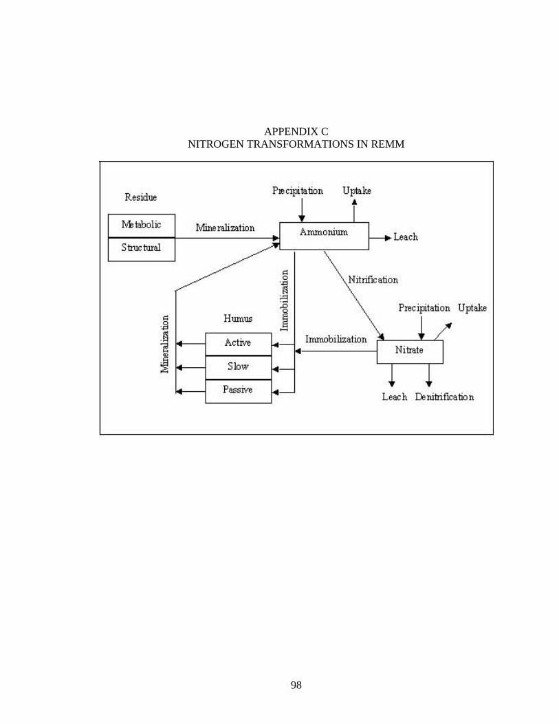
98
APPENDIX C NITROGEN TRANSFORMATIONS IN REMM
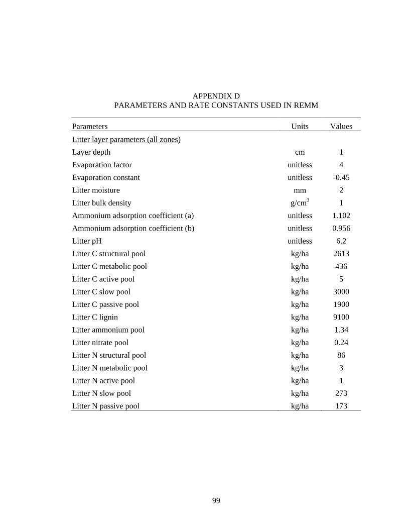
99
APPENDIX D PARAMETERS AND RATE CONSTANTS USED IN REMM
Parameters Units Values Litter layer parameters (all zones) Layer depth cm 1 Evaporation factor unitless 4 Evaporation constant unitless -0.45 Litter moisture mm 2 Litter bulk density g/cm3 1 Ammonium adsorption coefficient (a) unitless 1.102 Ammonium adsorption coefficient (b) unitless 0.956 Litter pH unitless 6.2 Litter C structural pool kg/ha 2613 Litter C metabolic pool kg/ha 436 Litter C active pool kg/ha 5 Litter C slow pool kg/ha 3000 Litter C passive pool kg/ha 1900 Litter C lignin kg/ha 9100 Litter ammonium pool kg/ha 1.34 Litter nitrate pool kg/ha 0.24 Litter N structural pool kg/ha 86 Litter N metabolic pool kg/ha 3 Litter N active pool kg/ha 1 Litter N slow pool kg/ha 273 Litter N passive pool kg/ha 173
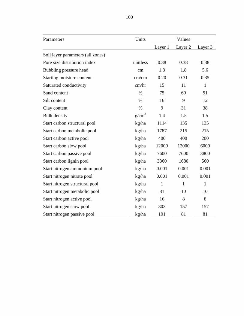
100
Parameters Units Values Layer 1 Layer 2 Layer 3 Soil layer parameters (all zones) Pore size distribution index unitless 0.38 0.38 0.38 Bubbling pressure head cm 1.8 1.8 5.6 Starting moisture content cm/cm 0.20 0.31 0.35 Saturated conductivity cm/hr 15 11 1 Sand content % 75 60 51 Silt content % 16 9 12 Clay content % 9 31 38 Bulk density g/cm3 1.4 1.5 1.5 Start carbon structural pool kg/ha 1114 135 135 Start carbon metabolic pool kg/ha 1787 215 215 Start carbon active pool kg/ha 400 400 200 Start carbon slow pool kg/ha 12000 12000 6000 Start carbon passive pool kg/ha 7600 7600 3800 Start carbon lignin pool kg/ha 3360 1680 560 Start nitrogen ammonium pool kg/ha 0.001 0.001 0.001 Start nitrogen nitrate pool kg/ha 0.001 0.001 0.001 Start nitrogen structural pool kg/ha 1 1 1 Start nitrogen metabolic pool kg/ha 81 10 10 Start nitrogen active pool kg/ha 16 8 8 Start nitrogen slow pool kg/ha 303 157 157 Start nitrogen passive pool kg/ha 191 81 81
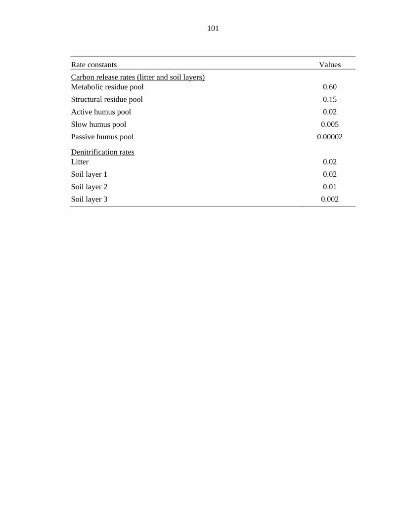
101
Rate constants Values Carbon release rates (litter and soil layers) Metabolic residue pool 0.60 Structural residue pool 0.15 Active humus pool 0.02 Slow humus pool 0.005 Passive humus pool 0.00002
Denitrification rates Litter 0.02 Soil layer 1 0.02 Soil layer 2 0.01 Soil layer 3 0.002
102
LIST OF REFERENCES
Altier, L.S., Lowrance, R.R., Williams, R.G., Inamdar, S.P., Bosch, D.D., Sheridan, J.M., Hubbard, R.K., Thomas, D.L. 2002. Riparian Ecosystem Management Model (REMM): simulator for ecological processes in riparian zones. United States Department of Agriculture, Agricultural Research Service, Conservation Research Report 46.
American Public Health Association. 1992. Standard Methods for the Examination of Water and Wastewater, 20th edition. Washington, D.C.
Auble, G.T., Friedman, J.M., Scott, M.L. 1994. Relating riparian vegetation to present and future streamflows. Ecological Applications 4, 544-554.
Band, L.E., Tague, C.L., Groffman, P., Belt, K. 2001. Forest ecosystem processes at the watershed scale: hydrological and ecological controls of nitrogen export. Hydrological Processes 15: 2013-2028.
Basnyat, P., Teeter, L., Flynn, K., Lockaby, B. 1999. Relationships between landscape characteristics and nonpoint source pollution inputs to coastal estuaries. Environmental Management 23: 539-549.
Berg, B., Staaf, H. 1981. Leaching, accumulation and release of nitrogen in decomposing litter. In Clark, F.E., Rosswall, T. (editors), Terrestrial Nitrogen Cycles. Ecological Bulletins (Stockholm) 33: 163-178.
Bernal, S., Butturini, A., Nin, E., Sabater, F., Sabater, S. 2003. Leaf litter dynamics and nitrous oxide emission in a mediterranean riparian forest: implications for soil nitrogen dynamics. Journal of Environmental Quality 32: 191-197.
Beschta, R.L., Jackson, W.L. 1979. The intrusion of fine sediments into a stable gravel bed. Journal of the Fisheries Research Board of Canada 36: 207-210.
Bhat S., Jacobs, J.M. (Department of Civil Engineering, University of New Hampshire), Hatfield, K. (Department of Civil and Coastal Engineering, University of Florida), Prenger, J. Ecological indicators in forested watersheds in Fort Benning, GA: relationship between land use and stream water quality. Ecological Indicators. Accepted pending revision.
Biggs, B.J.F. 1996. Hydraulic habitat of plants in streams. Regulated Rivers: Research and Management 12: 131-144.
103
Biggs, B.J.F. 2000. Eutrophication of streams and rivers: dissolved nutrient-chlorophyll relationships for benthic algae. Journal of the North American Benthological Society 19: 17-31.
Biggs, B.J.F., Close, M.E. 1989. Periphyton biomass dynamics in gravel bed rivers: the relative effects of flows and nutrients. Freshwater Biology 22: 209-231.
Biggs, B.J.F., Smith, R.A., Duncan, M.J. 1999. Velocity and sediment disturbance of periphyton in headwater streams: biomass and metabolism. Journal of the North American Benthological Society 18: 144-163.
Biggs, B.J.F., Stokseth, S. 1996. Hydraulic habitat preferences for periphyton in rivers. Regulated Rivers: Research and Management 12: 251-261.
Binkley, D. 1986. Forest Nutrition Management. John Wiley & Sons, New York.
Bocock, K.L., Gilbert, O., Capstick, C.K., Twinn, D.C., Waid, J.S., Woodman, M.J. 1960. Changes in leaf litter when placed on the surface of soils with contrasting humus types. I. Losses in dry weight of oak and ash leaf litter. Journal of Soil Science 11:1-9.
Bolstad, P.V., Swank, W.T. 1997. Cumulative impacts of land use on water quality in a southern Appalachian watershed. Journal of American Water Resources Association 33: 519-533.
Bosch, D.D., Sheridan, J.M., Lowrance, R.R. 1996. Hydraulic gradients and flow rates of a shallow coastal plain aquifer in a forested riparian buffer. Transactions of the American Society of Agricultural Engineers 39: 865-871.
Bren, L.J. 1992. Tree invasion of an intermittent wetland in relation to changes in the flooding frequency of the River Murray, Australia. Australian Journal of Ecology 17: 395-408.
Brinson, M.M., Bradshaw, H.D., Holmes, R.N., Elkins, Jr., J.B. 1980. Litterfall, stemflow, and throughfall nutrient fluxes in an alluvial swamp forest. Ecology 61: 827-835.
Bryant, M.L., Bhat, S., Jacobs, J.M. In Press. Characterization and modeling of throughfall temporal variability for forest communities in the southeastern U.S. Journal of Hydrology.
Bubb, K.A., Xu, Z.H., Simpson, J.A., Saffigna, P.G. 1998. Some nutrient dynamics associated with litterfall and litter decomposition in hoop pine plantations of southeast Queensland, Australia. Forest Ecology and Management 110: 343-352.
Cairns, Jr., J., McCormick, P.V., Neiderlehner, B.R. 1993. A proposed framework for developing indicators for ecosystem health. Hydrobiologia 263: 1-44.
104
Chapman, R.J., Hinckley, T.M., Lee, L.C., Teskey, R.O. 1982. Impact of water level changes on woody riparian and wetland communities. Vol. 10. Kearneysville (WV), US Fish & Wildlife Service. Publication No. OBS-82/83.
Campbell, G.S. 1974. A simple method for determining unsaturated conductivity from moisture retention data. Soil Science 117: 311-314.
Christ, M.J., David, M.B. 1996. Dynamics of extractable organic carbon in Spodosol forest floors. Soil Biology and Biochemistry 28: 1171-1179.
Cirmo, C.P., McDonnell, J.J. 1997. Linking the hydrologic and biogeochemical controls of nitrogen transport in near-stream zones of temperate-forested catchments: a review. Journal of Hydrology 199: 88-120.
Clausen, B., Biggs, B.J.F. 1997. Relationships between benthic biota and hydrological indices in New Zealand streams. Freshwater Biology 38: 327-342.
Clausen, B., Biggs, B.J.F. 2000. Flow indices for ecological studies in temperate streams: groupings based on covariance. Journal of Hydrology 237: 184-197.
Cleveland, C.C., Neff, J.C., Townsend, A.R., Hood, E. 2004. Composition, dynamics, and fate of leached dissolved organic matter in terrestrial ecosystems: results from a decomposition experiment. Ecosystems 7: 275-285.
Close, M.E., Davies-Colley, R.J. 1990. Baseflow chemistry in New Zealand rivers 2. influence of environmental factors. New Zealand Journal of Marine and Freshwater Research 24: 343-356.
Cole, D.W., Rapp, M. 1981. Elemental cycling in forest ecosystems. In Reichle, D.E. (editor). Dynamic Properties of Forest Ecosystems. International Biological Programme 23. Cambridge University Press, London, pp. 341-409.
Closs, G.P., Lake, P.S. 1996. Drought, differential mortality and the coexistence of a native and an introduced fish species in a southeast Australian intermittent stream. Environmental Biology of Fishes 47: 17-26.
Cobb, D.G., Galoway, T.D., Flannagan, J.F. 1992. Effects of discharge and substrate stability on density and species composition of stream insects. Canadian Journal of Fisheries and Aquatic Sciences 49: 1788-1795.
Colwell, R.K. 1974. Predictability, constancy, and contingency of periodic phenomena. Ecology 5: 1148-1153.
Conner, W.H., Day, Jr., J.W. 1976. Productivity and composition of a baldcypress-water tupelo site and a bottomland hardwood site in a Louisiana swamp. American Journal of Botany 63: 1354-1364.
105
Crockford, R.H., Richardson, D.P. 1998. Litterfall, litter and associated chemistry in a dry sclerophyll eucalypt forest and a pine plantation in southeastern Australia: 1. litterfall and litter. Hydrological Processes 12: 365-384.
Cummins, K.W. 1974. Structure and function of Stream ecosystems. BioScience 24: 631-641.
Currie, W.S., Aber, J.D., McDowell, W.H., Boone, R.D., Magill, A.H. 1996. Vertical transport of dissolved organic C and N under long-term N amendments in pine and hardwood forests. Biogeochemistry 35: 471-505.
Dale, V.H., Beyeler, S.C. 2001. Challenges in the development and use of ecological indicators. Ecological Indicators 1: 3-10.
Dale, V.H., Beyeler, S.C., Jackson, B. 2002. Understory vegetation indicators of anthropogenic disturbance in longleaf pine forests at Fort Benning, Georgia, USA. Ecological Indicators 1: 155-170.
Davies-Colley, R.J., Quinn, J.M. 1998. Stream lighting in five regions of North Island, New Zealand: control by channel size and riparian vegetation. New Zealand Journal of Marine and Freshwater Research 32: 591-606.
Fisher, S.G. 1983. Succession in streams. In Barnes, J.R., Minshall, G.W. (editors), Stream Ecology: Application and Testing of General Ecological Theory. Plenum Press, New York.
Fisher, D.S., Steiner, J.L., Endale, D.M., Stuedemann, J.A., Schomberg, H.H., Franzluebbers, A.J., Wilkinson, S.R. 2000. The relationship of land use practices to surface water quality in the Upper Oconee watershed of Georgia. Forest Ecology and Management 128: 39-48.
Fox, D.G. 1981. Judging air quality model performance: a summary of the AMS workshop on dispersion model performance. Bulletin of American Meteorological Society 62: 599-609.
Frick, E.A., Hippe, D.J., Buell, G.R., Couch, C.A., Hopkins, E.H., Wangsness, D.J., Garrett, J.W. 1998. Water quality in the Apalachicola-Chattahoochee-Flint river basin, Georgia, Alabama, and Florida, 1992–95. U.S. Geological Survey Circular-1164.
Furniss, M.J., Roeloffs, T.D., Yee, C.S. 1991. Road construction and maintenance. In Meehan, W.R. (editor). Influences of forest and rangeland management on salmonid fishes and their habitats. Special publication 19. American Fisheries Society, Bethesda, Maryland. pp. 297-323.
Garten, Jr., C.T., Ashwood, T.L., Dale, V.H. 2003. Effect of military training on indicators of soil quality at Fort Benning, Georgia. Ecological Indicators 3: 171-179.
106
Gjessing, E., Lygren, E., Berglind, L., Gulbrandsen, T., Skanne, R. 1984. Effect of highway runoff on lake water quality. Science of the Total Environment 33: 247-257.
Gosz, J.R., Likens, G.E., Bormann, F.H. 1972. Nutrient content of litter fall on the Hubbard Brook experimental forest. Ecology 53: 769-784.
Gosz, J.R., Likens, G.E., Borman. F.H. 1973. Nutrient release from decomposing leaf and branch litter in the Hubbard Brook forest, New Hampshire. Ecological Monographs 443:173-191.
Grimm, N.B., Fisher, S.G. 1992. Responses of arid-land streams to changing climate. In Firth, P. and Fisher, S.G. (editors). Global Climate Change and Freshwater Ecosystems. Springer, New York, pp. 211-233.
Hanson, D.L., Waters, T.F. 1974. Recovery of standing crop and production rate of a brook trout population in a flood-damaged stream. Transactions of American Fisheries Society 103: 431-439.
Harrel, R.C., Dorris, T.C. 1968. Stream order, morphometry, physio-chemical conditions, and community structure of benthic microinvertibrates in an interminnent stream system. American Naturalist 80: 221-251.
Harris, M.M., Safford, L.O. 1996. Effects of season and four tree species on soluble carbon content in fresh and decomposing litter of temperate forests. Soil Science, 161: 130-135.
Heath, G.W., Arnold, M.K., Edwards, C.A. 1966. Studies in leaf litter breakdown. I. Breakdown rates of leaves of different species. Pedobiologia 6: 1-12.
Helvey, J.D., Kochenderfer, J.N. 1990. Soil density and moisture content on two unused forest roads during first 30 months after construction. Research paper NE-629. U.S. Forest Service. Northeast Forest Experiment Station, Broomhall, Pennsylvania.
Hemphill, N., Cooper, S.D. 1983. The effect of physical disturbance on the relative abundances of two filter-feeding insects in a small stream. Oecologia 58: 378-383.
Herbohn, J.L., Congdon, R.A. 1998. Ecosystem dynamics at disturbed and undisturbed sites in North Queensland wet tropical rain forest. III. nutrient returns to the forest floor through litterfall. Journal of Tropical Ecology 14: 217-229.
Hill, A.R. 1981. Streams phosphorus exports from catchments with contrasting land uses in southern Ohio. Water Resources Bulletin 17: 627-634.
Hongve, D. 1999. Production of dissolved organic carbon in forested catchments. Journal of Hydrology 224: 91-99.
107
Horwitz, R.J. 1978. Temporal variability patterns and the distributional patterns of stream fishes. Ecological Monographs 48: 307-321.
Houser, J.N. (Oak Ridge National Laboratory, Oak Ridge, TN), Mulholland, P.J. (Oak Ridge National Laboratory, Oak Ridge, TN), Maloney, K.O. Catchment disturbance and stream metabolism: patterns in stream respiration and gross primary production along a gradient of upland soil and vegetation disturbance. Unpublished manuscript.
Hunsaker, C.T., Levine, D.A. 1995. Hierarchical approaches to the study of water quality in rivers. BioScience 45: 193-203.
Hynes, H.B.N. 1960. The Biology of Polluted Waters, Liverpool University Press, Liverpool.
Inamdar, S.P., Sheridan, J.M., Williams, R.G., Bosch, D.D., Lowrance, R.R., Altier, L.S., Thomas, D.L. 1999a. Riparian Ecosystem Management Model (REMM): I. testing of the hydrologic component for a Coastal Plain riparian system. American Society of Agricultural Engineers 42: 1679-1689.
Inamdar, S.P., Lowrance, R.R., Altier, L.S., Williams, R.G., Hubbard, R.K. 1999b. Riparian Ecosystem Management Model (REMM): II. testing of the water quality and nutrient cycling component for a Coastal Plain riparian system. American Society of Agricultural Engineers 42: 1691-1707.
Iverson, R.M., Hinckley, B.S., Webb, R.M., Hallet, B. 1981. Physical effects of vehicular disturbance on arid landscapes. Science 212: 915-917.
Johnes, P., Moss, B., Phillips, G. 1996. The determination of total nitrogen and total phosphorous concentrations in freshwaters from land use, stock headage and population data: testing a model for use in conservation and water quality management. Freshwater Biology 36: 451-473.
Johnson, L.B., Richards, C., Host, G.E., Arthur, J.W. 1997. Landscape influences on water chemistry in midwestern stream ecosystems. Freshwater Biology 37: 193-208.
Jones, J.A., Grant, G.E. 1996. Cumulative effects of forest harvest on peak streamflow in the western cascades of Oregon. Water Resources Research 32: 959-974.
Jowett, I.G., Duncan, M.J. 1990. Flow variability in New Zealand rivers and its relationship to in-stream habitat and biota. New Zealand Journal of Marine and Freshwater Research 24: 305-317.
Junk, W.J., Bayley, P.B., Sparks, R.E. 1989. The flood pulse concept in river-floodplain systems. Canadian Special Publication of Fisheries and Aquatic Sciences 106: 110-127.
108
Karr, J.R., Chu, E.W. 1999. Restoring Life in Running Waters: Better Biological Monitoring. Island Press, Washington, D.C.
Keller, E.A., Swanson, F.J. 1979. Effects of large organic material on channel form and fluvial processes. Earth Surface Processes and Landforms 4: 351-380.
Lemmon, P. E. 1956. A spherical densiometer for estimating forest overstory density. Forest Science 2: 314-320.
Leopold, L.B., Wolman, M.G., Miller, J.P. 1964. Fluvial processes in geomorphology. W.H. Freeman and Sons, San Francisco.
Lowrance, R. 1992. Groundwater nitrate and denitrification in a coastal plain riparian forest. Journal of Environmental Quality 21: 401-405.
Lowrance, R.R., Altier, L.S., Williams, R.G., Inamdar, S.P., Sheridan, J.M., Bosch, D.D., Hubbard, R.K., Thomas, D.L. 2000. REMM: the riparian ecosystem management model. Journal of Soil and Water Conservation 55: 27-34.
Lowrance, R., Todd, R.L., Asmussen, L.E. 1984. Nutrient cycling in an agricultural watershed: II. Streamflow and artificial drainage. Journal of Environmental Quality 13: 27-32.
Maloney, K.O., Mulholland, P.J., Feminella, J.W. In Press. Influence of catchment-scale military land use on physicochemical conditions in small Southeastern Plains streams (USA). Environmental Management.
McCuen, R.H. 1998. Hydrologic Analysis and Design. Pearson Prentice Hall, Upper Saddle River, NJ.
McDowell, W.H., Fisher, S.G. 1976. Autumnal processing of dissolved organic matter in a small woodland stream ecosystem. Ecology 57: 561-569.
McDowell, W.H., Likens, G.E. 1988. Origin, composition, and flux of dissolved organic carbon in the Hubbard Brook Valley. Ecological Monographs 58: 177-195.
McGill, W.B., Hunt, H.W., Woodmansee, R.G., Reuss, J.O. 1981. PHOENIX, a model of the dynamics of carbon and nitrogen in grassland soils. In Clark, F.E., Rosswall, T. (editors). Terrestrial Nitrogen Cycles. Ecological Bulletin (Stockholm) 33: 49-115.
Meador, M.R., Goldstein, R.M. 2003. Assessing water quality at large geographic scales: relations among land use, water physicochemistry, riparian condition, and fish community structure. Environmental Management 31: 504-517.
Meentemeyer, V., Box, E.O., Thompson, R. 1982. World patterns and amounts of terrestrial plant litter production. Bioscience 32:125-128.
109
Meffe, G.K. 1984. Effects of abiotic disturbance on coexistence of predator and prey fish species. Ecology 65: 1525-1534.
Meffe, G.K., Minckley, W.L. 1987. Persistence and stability of fish and invertebrate assemblages in a repeatedly disturbed Sonoran Desert stream. American Midland Naturalist 117: 177-191.
Meyer, J.L., Wallace, J.B. Eggert, S.L. 1998. Leaf litter as a source of dissolved organic carbon in streams. Ecosystems 1: 240-249.
Michalzik, B., Kalbitz, K., Park, J.H., Solinger, S., Matzner, E. 2001. Fluxes and concentrations of dissolved organic carbon and nitrogen – a synthesis for temperate forests. Biogeochemistry 52: 173-205.
Milchunas, D.G., Schultz, K.A., Shaw, R.B. 1999. Plant community response to disturbance by mechanized military maneuvers. Journal of Environmental Quality 28: 1533-1547.
Minckley, W.L., Deacon, J.E. 1991. Battle Against Extinction: Native Fish Management in the American West. University of Arizona Press, Tucson, AZ.
Minckley, W.L., Meffe, G.K. 1987. Differential selection by flooding in stream-fish communities of the arid American Southwest. In Matthews, W.J., Heins, D.C. (editors). Community and Evolutionary Ecology of North American Stream Fishes. University of Oklahoma Press, Norman, OK.
Minshall, G.W. 1984. Aquatic insect-substratum relationships. In Resh, V.H. and Rosenberg, D.M. (editors). The Ecology of Aquatic Insects. Praeger Scientific, pp. 358-400.
Moore, K.M.S., Gregory, S.V. 1988. Response of young-of-the-year cutthroat trout to manipulations of habitat structure in a small stream. Transactions of the American Fisheries Society 117: 162-170.
Moss, D., Furse, M.T., Wright, J.F., Armitage, P.D. 1987. The prediction of the macroinvertebrate fauna of unplotted running-water sites in Great Britain using environmental data. Freshwater Biology 17: 41-52.
Mulholland, P.J. 1981. Organic carbon flow in a swamp-stream ecosystem. Ecological Monographs 51: 307-322.
Nakamura, F., Swanson, F.J., Wondzell, S.M. 2000. Disturbance regimes of stream and riparian systems- a disturbance cascade perspective. Hydrological Processes 14: 2849-2860.
Nash, J.E., Sutcliffe, V. 1970. River flow forecasting through conceptual models, I. a discussion of principles. Journal of Hydrology 10: 282-290.
110
National Research Council (NRC). 2000. Ecological Indicators for the Nation. National Academy Press, Washington, D.C.
Natural Resources Conservation Service (NRCS). 1995. Riparian Forest Buffer, 391. Model State Standard and General Specifications. NRCS Watershed Science Institute. Seattle, WA.
Nykvist, N. 1961. Leaching and decomposition of litter. III. experiments on leaf litter of Betula verrucosa. Oikos 12: 249-263.
Ohte, N., Tokuchi, N., Katsuyama, M., Hobara, S., Asano, Y., Koba, K. 2003. Episodic increases in nitrate concentrations in streamwater due to the partial dieback of a pine forest in Japan: runoff generation processes control seasonality. Hydrological Processes 17: 237-249.
Olden, J.D., Poff, N.L. 2003. Redundancy and the choice of hydrologic indices for characterizing streamflow regimes. River Research and Applications 19: 101-121.
O’Neill, R.V., Hunsaker, C.T., Jones, K.B., Riitters, K.H., Wickham, J.D., Schwartz, P.M., Goodman, I.A., Jackson, B.L., Baillargeon, W.S. 1997. Monitoring environmental quality at the landscape scale. BioScience 47: 513-519.
Osborne, L., Wiley, M. 1988. Empirical relationships between land use/cover patterns and stream water quality in an agricultural watershed. Journal of Environmental Management 26: 9-27.
Park, J., Matzner, E. 2003. Controls on the release of dissolved organic carbon and nitrogen from a deciduous forest floor investigated by manipulations of aboveground litter inputs and water flux. Biogeochemistry 66: 265-286.
Parton, W.J., Schimel, D.S., Cole, C.V., Ojima, D.S. 1987. Analysis of factors controlling soil organic matter levels in great plains grasslands. Soil Society of America Journal 51: 1173-1179.
Pastor, J., Post, W.M. 1986. Influence of climate, soil moisture, and succession on forest carbon and nitrogen cycles. Biogeochemistry 2: 3-27.
Perkins, H.F., Hook, J.E., Barbour, N.W. 1986. Soil characteristics of selected areas of the Coastal Plain experiment stations, University of Georgia. Research Bulletin 346.
Perry, C.D., Vellidis, G., Lowrance, R., Thomas, D.L. 1999. Watershed-scale water quality impacts of riparian forest management. Journal of Water Resources Planning and Management 125: 117-125.
Pettit, N.E., Froend, R.H., Davies, P.M. 2001. Identifying the natural flow regime and the relationship with riparian vegetation for two contrasting western Australian rivers. Regulated Rivers: Research and Management 17: 201-215.
111
Petts, G.E. (editor). 1984. Impounded Rivers: Perspectives for Ecological Management. Wiley, Chichester.
Piegay, H., Landon, N. 1997. Promoting ecological management of riparian forest on the Drome River, France. Aquatic Conservation: Marine and Freshwater Ecosystems 7: 287-304.
Poff, N.L. 1996. A hydrogeography of unregulated streams in the United States and an examination of scale-dependence in some hydrological descriptors. Freshwater Biology 36: 101-121.
Poff, N.L., Allan, J.D. 1995. Functional organization of stream fish assemblages in relation to hydrological variability. Ecology 76: 606-627.
Poff, N.L., Allan, J.D., Bain, M.B., Karr, J.R., Prestegaard, K.L., Richter, B.D., Sparks, R.E., Stromberg, J.C. 1997. The natural flow regime: a paradigm for river conservation and restoration. BioScience 47: 769-784.
Poff, N.L., Ward, J.V. 1989. Implications of streamflow variability and predictability for lotic community structure: a regional analysis of streamflow patterns. Canadian Journal of Fisheries and Aquatic Sciences 46: 1805-1818.
Polglase, P.J., Attiwill, P.M. 1992. Nitrogen and phosphorus cycling in relation to stand age of Eucalyptus regnans F. Muell. I. return from plant to soil in litterfall. Plant and Soil 142: 157-166.
Power, M.E., Stewart, A.J. 1987. Disturbance and recovery of an algal assemblage following flooding in an Oklahoma stream. American Midland Naturalist 117: 333-345.
Qualls, R.G., Haines, B.L., Swank, W.T. 1991. Fluxes of dissolved organic nutrients and humic substances in a deciduous forest. Ecology 72: 254-266.
Quist, M.C., Fay, P.A., Guy, C.S., Knapp, A.K., Rubenstein, B.N. 2003. Military training effects on terrestrial and aquatic communities on a grassland military installation. Ecological Applications 13: 432-442.
Resh, V.H., Brown, A.V., Covich, A.P., Gurtz, M.E., Li, H.W., Minshall, G.W., Reice, S.R., Sheldon, A.L., Wallace, J.B., and Wissmar, R. 1988. The role of disturbance in stream ecology. Journal of the North American Benthological Society 7: 433-455.
Richards, C., Haro, R.J., Johnston, L.B., Host, G.E. 1997. Watershed and reach-scale properties as indicators of macroinvertebrate species traits. Freshwater Biology 37: 219-230.
Richards, C., Host, G.E. 1994. Examining land use influences on stream habitats and macroinvertebrates: a GIS approach. Water Resources Bulletin 30: 729-738.

112
Richards, C., Johnston, L.B., Host, G.E. 1996. Assessing the influence of landscape-scale watershed features on physical habitat and stream biota. Canadian Journal of Fisheries and Aquatic Sciences 53: 295-311.
Richter, B.D., Baumgartner, J.V., Powell, J., Braun, D.P. 1996. A method for assessing hydrologic alteration within ecosystems. Conservation Biology 10: 1163-1174.
Rogers, H.M. 2002. Litterfall, decomposition and nutrient release in a lowland tropical rain forest, Morobe Province, Papua New Guinea. Journal of Tropical Ecology 18: 449-456.
Schiemer, F., Zalewski, M., Thorpe, J.E. (editors). 1995. The Importance of Aquatic-Terrestrial Ecotones for Freshwater Fish. Developments in Hydrobiology. Volume 105. Kluwer, Dordrecht.
Schindler, D., Bayley, S. 1993. The biosphere as an increasing sink for atmospheric carbon: estimates from increasing nitrogen deposition. Global Biogeochemistry Cycles 7: 717-734.
Schlesinger, W.H. 1978. Community structure, dynamics and nutrient cycling in the Okefenoke cypress swamp forest. Ecological Monographs 48: 43-65.
Schlosser, I.J. 1985. Flow regime, juvenile abundance, and the assemblage structure of stream fishes. Ecology 66: 1484-1490.
Scott, M.L., Friedman, J.M., Auble, G.T. 1996. Fluvial processes and the establishment of bottomland trees. Geomorphology 14: 327-339.
Semkin, R.G., Jeffries, D.S., Clair, T.A. 1994. Hydrochemical methods and relationships for study of stream output from small catchments. In Molden, B. and Cerny, J. (editors). Biogeochemistry of Small Catchments: A Tool for Environmental Research. John Wiley and Sons, Chichester, pp. 163-188.
Sheridan, J.M., Lowrance, R.R., Henry, H.H. 1996. Surface flow sampler for riparian studies. Applied Engineering in Agriculture 12: 183-188.
Shirmohammadi, A.J., Sheridan, J.M., Knisel, W.G. 1984. An approximate method for partitioning daily streamflow data. Journal of Hydrology 74: 335-354.
Shure, D.J., Gottschalk, M.R. 1985. Litter-fall patterns within a floodplain forest. American Midland Naturalist 114: 98-111.
Sidle, R.C., Pearce, A.J., O’Loughlin, C.L. 1985. Soil mass movement- influence of natural factors and land use. American Geophysical Union Water Resources Monograph 11, American Geophysical Union, Washington, D.C.
113
Silveira, M.L., Reddy, K.R. (Department of Soil and Water Science, University of Florida), Comerford, N.B. (Department of Soil and Water Science, University of Florida). Litter decomposition and soluble organic carbon and nitrogen release in a forested ecosystem. Unpublished manuscript.
Singh, K.P., Singh, P.K., Tripathi, S.K. 1999. Litterfall, litter decomposition and nutrient release patterns in four native tree species raised on coal mine spoil at Singrauli, India. Biology and Fertility of Soils 29: 371-378.
Sliva, L., Williams, D.D. 2001. Buffer zones versus whole catchment approaches to studying land use impact on river water quality. Water Research 35: 3462-3472.
Sponseller, R.A., Benfield, E.F., Valett, H.M. 2001. Relationships between land use, spatial scale and stream microinvertibrate communities. Freshwater Biology 46: 1409-1424.
Stone, J. J., Hawkins, R.H., Shirley, E.D. 1994. An approximate form of the Green Ampt infiltration equation. ASCE Journal of Irrigation and Drainage 120: 128-137.
Stromberg, J.C., Fry, J., Patten, D.T. 1997. Marsh development after large floods in an alluvial, arid-land river. Wetlands 17: 292-300.
Tipping, E., Woof, C., Rigg, E., Harrison, A.F., Inneson, P., Taylor, K., Benham, D., Poskitt, J., Rowland, A.P., Bol, R., Harkness, D.D. 1999. Climatic influences on the leaching of dissolved organic matter from upland UK moorland soils investigated by a field manipulation experiment. Environment International 25: 83-95.
Thomas, D.L., Beasley, D.B. 1986. A physically-based forest hydrology model. I: development and sensitivity of components. Transactions of the ASAE 29: 962-972.
Thurow, T.L., Warren, S.D., Carlson, D.H. 1993. Tracked vehicle traffic effects on the hydrologic characteristics of central Texas rangeland. Transactions of the American Society of Agricultural Engineers 36: 1645-1650.
Ukonmaanaho, L., Starr, M. 2001. The importance of leaching from litter collected in litterfall traps. Environmental Monitoring and Assessment 66: 129-146.
Vannote, R.L., Minshall, G.W., Cummins, K.W., Sedell, J.R., Cushing, C.E. 1980. The river continuum concept. Canadian Journal of Fisheries and Aquatic Sciences 37: 130-137.
Vitousek, P.M., Aber, J.D., Howarth, R.W., Likens, G.E., Matson, P.A., Schindler, D.W., Schlesinger, W.H., Tilman, D.G. 1997. Human alteration of the global nitrogen cycle: sources and consequences. Ecological Applications 7: 737-750.
114
Wallace, J.B., Benke, A.C. 1984. Quantification of wood habitat in subtropical coastal plains streams. Canadian Journal of Fisheries and Aquatic Sciences 41: 1643-1652.
Wang, L., Lyons, J., Kanehl, P., Bannerman, R. 2001. Impacts of urbanization on stream habitat and fish across multiple spatial scales. Environmental Management 28: 255-266.
Welcomme, R.L. 1992. River conservation - future prospects. In Boon, P.J., Calow, P., and Petts, G.E. (editors). River Conservation and Management. John Wiley and Sons. New York.
Wemple, B.C., Jones, J.A., Grant, G.E. 1996. Channel network extension by logging roads in two basins, western Cascades, Oregon. Water Resources Bulletin 32: 1195-1207.
Whitecotton, R.C.A., David, M.B., Darmody, R.G., Price, D.L. 2000. Impact of foot traffic from military training on soil and vegetation properties. Environmental Management 26: 697-706.
Wilson, S.D. 1988. The effects of military tank traffic on prairie: a management model. Environmental Management 12: 397-403.
Wood, P.J., Agnew, M.D., Petts, G.E. 2000. Flow variations and macroinvertebrate community responses in a small groundwater-dominated stream in south-east England. Hydrological Processes 14: 3133-3147.
Zalewski, M. 1999. Minimising the risk and amplifying opportunities for restoration of shallow reservoirs. Hydrobiologia 395/396: 107-114.
Zalewski, M. 2000. Ecohydrology- the scientific background to use ecosystem properties as management tools toward sustainability of water resources, Ecological Engineering 16: 1-8.
Zalewski, M., Janauer, G.A., Jolankai, G. 1997. Ecohydrology: a new paradigm for the sustainable use of aquatic resources. In Conceptual Background, Working Hypothesis, Rationale and Scientific Guidelines for the Implementation of the IHP-V Projects 2.3/2.4. UNESCO, Paris Technical Documents in Hydrology No. 7.

115
BIOGRAPHICAL SKETCH
Shirish Bhat was born in Pokhara, Nepal, on January 12, 1968. He graduated with
a bachelor’s degree in science from Tribhuvan University, Nepal, in 1989. He graduated
with his second bachelor’s degree in civil engineering from Regional Engineering
College, Warangal, India, in 1994. He worked as a civil engineer for the Canadian
Center for International Studies and Cooperation (CECI) in Nepal from July 1994 to
August 1995. He also worked as a civil engineer consultant for the Department of
National Parks and Wildlife Conservation, Government of Nepal, from September 1995
to August 1997. In Fall 1997, he began graduate studies in the Department of Civil and
Environmental Engineering at South Dakota State University, Brookings, South Dakota,
USA, and obtained his master’s degree (thesis option) in Summer 1999. Shirish joined
the Department of Civil and Coastal Engineering at the University of Florida, Florida,
USA, in the Fall of 1999 and will obtain his Ph.D. degree in Spring 2005 under the
supervision of Dr. Jennifer Jacobs and Dr. Kirk Hatfield. His primary research interests
include land use impacts on surface water quality and quantity, riparian area nutrient
dynamics, biogeochemistry of wetlands, and water resources management. He is a
student member of the American Geophysical Union (AGU) and the ASCE.