eco hydrology
DESCRIPTION
hidrologi lingkunganTRANSCRIPT

ECO-HYDROLOGY
In the last two decades the importance of hydrological processes in ecosystemsand the effects of plants on hydrological processes have become increasinglyapparent. These relationships can be grouped under the term ‘eco-hydrology’.
Eco-Hydrology introduces and explores diverse plant-water interactions in arange of environments. Leading ecologists and hydrologists present reviews ofthe eco-hydrology of drylands, wetlands, temperate and tropical rain forests,streams and rivers, and lakes. The authors provide background information onthe water relations of plants, from individual cells to stands together with an in-depth review of scale issues and the role of mathematical models inecohydrology.
Eco-Hydrology is the first book to offer an overview of the complexrelationships between plants and water across a range of terrestrial and aquaticenvironments. The text will prove invaluable as an introduction to hydrologists,ecologists, conservationists and others studying ecosystems, plant-life andhydrological processes.
Andrew Baird is lecturer in Physical Geography at the University ofSheffield, and Robert Wilby is senior lecturer in Physical Geography at theUniversity of Derby, and a project scientist at the National Center for AtmosphericResearch, Boulder, Colorado.

A VOLUME IN THE ROUTLEDGE PHYSICALENVIRONMENT SERIESEdited by Keith RichardsUniversity of Cambridge
The Routledge Physical Environment series presents authoritative reviews ofsignificant issues in physical geography and the environmental sciences. Theseries aims to become a complete text library, covering physical themes, specificenvironments, environmental change, policy and management as well asdevelopments in methodology, techniques and philosophy.
Other titles in the series:
ENVIRONMENTAL HAZARDS: ASSESSING RISK AND REDUCINGDISASTER K.Smith
WATER RESOURCES IN THE ARID REALM E.Anderson and C.Agnew
ICE AGE EARTH: LATE QUATERNARY GEOLOGY AND CLIMATE A.Dawson
THE GEOMORPHOLOGY OF DESERT DUNES N.Lancaster
SOILS AND ENVIRONMENT S.Ellis and A.Mellor
TROPICAL ENVIRONMENTS: THE FUNCTIONING AND MANAGEMENTOF TROPICAL ECOSYSTEMS M.Kellman and R.Tackaberry
MOUNTAIN WEATHER AND CLIMATE Roger G.Barry
Forthcoming:
TROPICAL FOREST ECOSYSTEMS S.Bruijnzeel and J.Proctor
ENVIRONMENTAL ISSUES IN THE MEDITERRANEAN J.Thornes and J.Wainwright
MOUNTAIN GEOGRAPHY D.Funnell and R.Parish
ECO-HYDROLOGY
Plants and water in terrestrial andaquatic environments
Edited by Andrew J.Baird and Robert L.Wilby
London and New York

First published 1999by Routledge
11 New Fetter Lane, London EC4P 4EE
Simultaneously published in the USA and Canadaby Routledge
29 West 35th Street, New York, NY 10001
Routledge is an imprint of the Taylor & Francis Group
This edition published in the Taylor & Francis e-Library, 2005.
“To purchase your own copy of this or any of Taylor & Francis or Routledge’s collection ofthousands of eBooks please go to www.eBookstore.tandf.co.uk.”
© 1999 Andrew J.Baird & Robert L.Wilby, selection and editorial matter; individual contributors,chapters
All rights reserved. No part of this book may be reprinted orreproduced or utilized in any form or by any electronic, mechanical,
or other means, now known or hereafter invented, includingphotocopying and recording, or in any information storage or
retrieval system, without permission in writing from the publishers.
British Library Cataloguing in Publication DataA catalogue record for this book is available from the British Library
Library of Congress Cataloging-in-Publication DataA catalog record is available on request
ISBN 0-203-98009-3 Master e-book ISBN
ISBN 0-415-16272-6 (hbk)ISBN 0-415-16273-4 (pbk)
CONTENTS
List of figures vi
List of tables xi
List of contributors xiii
Preface xiv
1 IntroductionANDREW J.BAIRD
1
2 Water relations of plantsMELVIN T.TYREE
10
3 Scales of interaction in eco-hydrological relationsROBERT L.WILBY AND DAVID S.SCHIMEL
36
4 Plants and water in drylandsJOHN WAINWRIGHT, MARK MULLIGAN AND JOHNTHORNES
72
5 Water and plants in freshwater wetlandsBRYAN D.WHEELER
119
6 Plants and water in forests and woodlandsJOHN ROBERTS
170
7 Plants and water in streams and riversANDREW R.G.LARGE AND KAREL PRACH
223
8 Plants and water in and adjacent to lakesROBERT G.WETZEL
253
9 ModellingANDREW J.BAIRD
284
10 The future of eco-hydrologyROBERT L.WILBY
327
Index 354

FIGURES
2.1 Drawing of a living cell with plasmalemma membrane adjacent to axylem conduit of cellulose. A: Hofler diagram. B: Representativedaily time course
13
2.2 A: A typical plant. B: Cross-section. C to F: Lower leaf surface 162.3 Relationship between change of gL relative to the maximum value and
various environmental factors 16
2.4 Correlation of daily water use of leaves and net radiation 182.5 A: Differences in root morphology and depth of root systems of
various species of prairie plant growing in a deep, well-aerated soil. B:A dicot root tip enlarged about 50×. C: Cross-section of monocot anddicot roots enlarged about 400×
20
2.6 The Ohm’s law analogy 222.7 Pressure profiles in three large trees 232.8 Vulnerability curves for various species 262.9 Solar energy budgets of leaves under different conditions 282.10 Solar energy budget of a uniform stand of plants 292.11 Solar energy budget values measured in a meadow 312.12 Effects of drought on transpiration, leaf water potential and stomatal
conductance 33
3.1 Conceptualisation of down-scaling and aggregation betweenatmospheric and hydrological models
39
3.2 Spatial and temporal scales of rainfall in relation to a range ofhydrological problems
42
3.3 Correlation decay curves for winter and summer daily rainfallbetween neighbouring stations across Europe
44
3.4 Definition of the representative elementary area (REA) 443.5 A: Aircraft measurements of sensible heat, latent heat and eddy
kinetic energy at a height of 100 m. B: A proposed clarification ofdifferent types of land surface based on organisational variability ofsurface cover
46
3.6 LANDS AT Thematic Mapper composite image showing variationsin land cover at A: the regional scale; B: the mesoscale; and C: thelocal scale
49
3.7 Simulated yield reduction curves for selected Lmax values followingtwenty years of eucalypt forest harvesting upstream of Tea-treeSwamp, Victoria, Australia
49
3.8 Forms of the theoretical scaling relationship between tree leaf areaand water flux
52
3.9 Frequency diagrams of wet day rainfall amounts at Kempsford in theCotswolds, UK
55
3.10 Schematic representation of a simple patch model includingdefinitions of all model parameters
60
3.11 Conceptual model showing the relationship between direct gradients,their environmental determinants and potential natural vegetation
62
3.12 Schematic illustration of the coupling of water, nitrogen cycling andcarbon in ecosystems
65
4.1 The aridification-desertification feedback loop 774.2 Changing seasonality of rainfall for Belmonte, central Spain, 1940–
1991 78
4.3 Rainfall variability for Belmonte, central Spain, 1940–1991 794.4 The effect of different spatial distributions of vegetation cover on
predicted erosion rate 84
4.5 Relationships between precipitation and sediment yield 864.6 Generalised relationships showing the mean annual sediment yield as
a function of A: mean annual precipitation; and B: mean annualrunoff
86
4.7 Proposed relationships relating annual precipitation to sediment yieldas a function of different temperatures
87
4.8 Markov transition probabilities of transitions of vegetation typesobserved in the Tenaghi Philippon core
99
4.9 Hydrological output of PATTERN model for matorral site withBelmonte rainfall data, 1940–1991
0
4.10 Leaf area index for main matorral functional types from PATTERNmodel using Belmonte rainfall data, 1940–1991
104
4.11 Plant structural properties for shrub functional type from PATTERNmodel using Belmonte rainfall data, 1940–1991
104
4.12 Output from PATTERN model for hill-slope biomass for three mainmatorral functional types for current CO2 and 2× CO2 greenhouserainfall scenario
104
5.1 Wetland categories and terms as used in this chapter 1206.1 The hydrological cycle in a tropical rain forest 1726.2 Interception ratios plotted against annual rainfall for interception
studies involving conifers and broadleaves in the UK 176
6.3 The relation between the rate of soil water depletion and the deficit ofavailable water under forests
189
6.4 Changes in stomatal conductance of several species in response tochanges in air humidity deficit
189
6.5 The dependence of relative surface conductance on solar radiation,specific humidity deficit, temperature and soil moisture deficit
194
vii
6.6 A: Downward cumulative leaf area index at Thetford Forest, UK. B:Vertical variation in leaf area density at Thetford Forest
201
6.7 Average diurnal curves of canopy conductance for the forest atReserva Ducke, Manaus, and Thetford Forest in a normal and a dryyear
201
6.8 Cumulative values of gross rainfall and rainfall interception loss atThetford Forest
201
6.9 The relationship between leaf stomatal conductance and air specifichumidity deficit for Piptadenia suaveolens and Pinus sylvestris
203
6.10 Change in transpiration rate of forest and bracken and their ratio inresponse to air humidity deficit, Thetford Forest, UK
203
6.11 Reserva Florestal Ducke, Manaus. A: Downward cumulative leaf areaindex of the tropical rain forest. B: Vertical variation in leaf areadensity
204
6.12 Cumulative values of gross rainfall and rainfall interception loss inthe Reserva Florestal Ducke, Manaus
206
6.13 Total water potential as a function of soil depth at the ReservaFlorestal Ducke, Manaus
208
6.14 Diurnal variation in stomatal conductance of some of the speciesaround the sampling tower at the Reserva Florestal Ducke, Manaus
208
6.15 Leaf area in each of five canopy layers and transpiration from eachlayer, Reserva Florestal Ducke, Manaus
210
7.1 Three-reach model system 2257.2 General relationship between Manning’s n and the velocity and
hydraulic radius product (VR) at constant biomass 227
7.3 Relationship between the biomass of Ranunculus penicillatus var.calcareus and Manning’s n
229
7.4 The roles played by rooted macrophytes in lowland streams 2317.5 Examples of species distribution in relation to flow type 248 7.6 Colonisation of rivers and streams in the Czech Republic by
Impatient glandulifera between 1940 and 1990 234
7.7 Relationship between number of species of water macrophyte andcurrent velocity for fifty-eight transects across the Sävåran River,northern Sweden
236
7.8 How flow affects macrophyte growth and survival 2377.9 Distribution of Hydrocharis morsus-ranae along a 100 km section of
the River Elbe in the Czech Republic, 1976–1996 238
7.10 Model showing influence of eutrophication on water plants 240711 The influence of the flood pulse within the river-floodplain complex 2448.1 Number of permanent lakes in the world in relation to lake area and
approximate mean water depth 254
8.2 Energy sources and sinks associated with the energy budget of lakes 2608.3 Idealised vertical distribution of oxygen concentrations and
temperature during the four main seasonal phases of an oligotrophic 262
viii
and a eutrophic dimictic lake that circulates completely twiceannually
8.4 Estimated number of lakes in the world in relation to the ratios ofpelagic to littoral and wetland portions of aquatic ecosystems
272
8.5 Annual average rates of photosynthesis and photosyntheticefficiencies of light utilisation by the emergent aquatic plant Juncuseffusus under conditions of natural variations in irradiance andtemperature in the Talladega Wetland Ecosystem, Hale County,Alabama
276
8.6 Variations in the transport of water laterally within sandy claysediments of the Talladega Wetland Ecosystem, Hale County,Alabama
276
8.7 Diurnal fluctuations in surface water levels within the TalladegaWetland Ecosystem, Hale County, Alabama
278
9.1 The hydrological cycle: a very simple conceptual model 2869.2 A conceptual model of hydrological stores and transfers at the
catchment scale 287
9.3 A physical model: a soil tank used for analysing overland flow anderosion on semi-arid slope surfaces
288
9.4 A saturated control volume for analysing flow through a soil 2899.5 A cross-section of soil in a floodplain aquifer 2919.6 A conceptual mathematical model, HYRROM, of catchment runoff 2949.7 A physically based, distributed catchment model: Système
Hydrologique Européen 296
9.8 River and adjacent floodplain 3029.9 Pictorial representation of a cross-section through the floodplain
shown in 302
9.10 Empirical model of water table behaviour in the floodplain shown in 3039.11 A simple physically based model of water table behaviour in the
floodplain shown in 305
9.12 A Darcy-Richards model for predicting water tables in the floodplainshown in
309
9.13 Rates of ponded infiltration as a function of time calculated usingequation (9.16)
316
9.14 Definition of the representative elementary volume (REV) 31910.1 A conceptualisation of humanity’s direct and indirect effect on the
Earth’s ecosystems 330
10.2 Critical sulphate loads for the Beacon Hill catchment, CharnwoodForest, Leicestershire, UK
333
10.3 Multi-scale measurement strategy used in BOREAS 33510.4 Time series of simulated and observed volume-weighted annual
average concentrations of selected variables in runoff of the Egilcatchment of the RAIN project
337
10.5 The marine biogeochemical cycle of dimethyl sulphide 341
ix

10.6 Examples of degraded landscapes in A: Moroccan dryland and B:Malaysian tropical moist forest
343
x
TABLES
3.1 Spatial scales in hydrology 383.2 Outstanding challenges to the confident application of statistical
downscaling techniques 56
3.3 Examples of topographically derived hydrometeorological variables 584.1 General characteristics of dryland climates 744.2 Features of poikilohydrous plants 824.3 The eco-hydrological consequences of vegetation clumping 834.4 The effect of data resolution on evapotranspiration estimates 935.1 Differences between the layers of a peat deposit 1456.1 The IGBP-DIS land cover classification 1716.2 Annual transpiration of different vegetation covers 1866.3 Percentage stand evapotranspiration from forest understorey 1896.4 Water balance components for Thetford Forest, UK, and Reserva
Ducke, Brazil 200
7.1 Basic four-fold classification of macrophytes of streams and rivers 2257.2 Potential areas of research relating to plants of streams and rivers 2458.1 Averages of rates of primary production of higher aquatic plants of
inland waters 255
8.2 Annual net primary productivity of aquatic communities on fertilesites in comparison with that of other communities
255
8.3 Comparison of the productivity and loading characteristics ofLawrence Lake, Michigan, and Mirror Lake, New Hampshire
265
8.4 Nitrogen mass balances of five streams in percentage of total in eachcategory
267
8.5 Average annual nitrogen budget for Mirror Lake, New Hampshire,1970–1975
269
8.6 Phosphorus budget for a deep, arctic tundra lake, Toolik Lake, Alaska 2708.7 Comparison of water loss from a stand of the emergent aquatic
macrophyte Phragmitis australis with that from open water 273
8.8 Representative rates of evapotranspiration by aquatic plants andcomparison with rates of evaporation from open water
274
10.1 Surface parameters derived from remotely sensed data 33710.2 The timescales for biological and physical processes involved in the
development of ecosystems on a newly produced bare area 342
10.3 Short-term and long-term approaches to soil problems in ecologicalrestoration
344

10.4 Rehabilitation techniques for surface waters affected by algae 346
xii
CONTRIBUTORS
Andrew R.G. Large, Department of Geography, University of Newcastle UponTyne, UK.Mark Mulligan, Department of Geography, King’s College London(University of London), UK.Karel Prach, Faculty of Biological Sciences, University of South Bohemia,Czech Republic.John M.Roberts, Hydrological Processes Division, Institute of Hydrology,Wallingford, Oxfordshire, UK.David S.Schimel, National Center for Atmospheric Research, Boulder,Colorado, US.John B.Thornes, Department of Geography, King’s College London(University of London), UK.Melvin T.Tyree, Aiken Forestry Services Laboratory, Burlington, Vermont,US.John Wainwright, Department of Geography, King’s College London(University of London), UK.Robert G.Wetzel, Department of Biological Sciences, University of Alabama,College of Arts and Sciences, Tuscaloosa, Alabama, US.Bryan D.Wheeler, Department of Animal and Plant Sciences, University ofSheffield, Sheffield, UK.
PREFACE
We live in a time when the boundaries between academic disciplines arebecoming increasingly blurred. Many contemporary environmental problems andimportant research questions can only be addressed by collaboration betweenallied disciplines. For example, the management of wetland ecosystems fornature conservation may involve ecologists working closely with hydrologists inorder to understand the water level and water quality requirements of a givenplant community in a particular wetland. Equally, the management of a wetlandfor nature conservation also requires an appreciation of which species andhabitats to conserve, and here we enter the realms of social science,environmental ethics and environmental law.
This volume is an attempt to formalise an area of overlap between twodisciplines, namely ecology and hydrology. In the last two decades, ecologistshave become increasingly aware of the importance of hydrological processes toecosystem functions. Although many workers accept simple conceptual modelssuch as the hydrosere (which shows a relationship between plants and theposition of the water table), there is still a lack of detailed understanding abouthow individual plants or assemblages of plants are affected by and, in turn,influence hydrological processes. Hydrologists have also become more aware ofthe effects of plants on hydrological processes. For example, in arid and semi-arid environments, hydrologists have found that the distribution of plants has aprofound effect on overland flow processes and erosion. Equally, the distributionand cover of plants is critically controlled by water availability.
Such relationships may be grouped under the term eco-hydrology. However,this term should not be confused with ‘hydro-ecology’, which is used in anarrower sense to describe the study of ecological and hydrological processes inrivers and floodplains. Although the term ‘eco-hydrology’ has been frequentlycoined by ecologists to describe interactions between water tables and plantdistributions in wetlands, it can be used to describe plant-water interactions inother environments. In dealing with eco-hydrology, this volume therefore coversa wider range of hydrological environments than is implied by ‘hydro-ecology’.Although this book aims to introduce the reader to some of the themes withineco-hydrology, it is not an introductory text in the usual sense. It is assumed that
readers have a good basic understanding of hydrology and ecology, andaccordingly the volume is pitched at advanced undergraduates and researcherscoming to the subject for the first time. Although this book is an edited collectionwe have adopted a slightly unconventiontal approach to its preparation. We feltthat it was impossible for one, two or even three authors to provide a sufficientlyexpert overview of the different areas within eco-hydrology. This necessitatedadopting a truly multi-author approach. In contrast to multi-author conferenceproceedings, which are now so common, the detailed structure and content of thebook were designed in advance and the authors carefully matched to theproposed chapters. However, one positive feature of conferences is that authorscan take on board constructive comments made by other delegates beforepublishing their work in the proceedings. In essence the refereeing base iswidened. Recognising this advantage, the authors of each chapter were invited bythe editors to an open workshop on eco-hydrology held at the University ofSheffield on 18 October 1997 and sponsored by the British Ecological Societyand the British Hydrological Society. The workshop was attended by over fiftyacademics, professional hydrologists and practising ecologists. The paperspresented at the meeting stimulated much useful discussion and feedback, andwe are indebted to all those who attended the workshop for making it a success.
In addition to the comments received at the workshop, each chapter was alsoindependently reviewed, and we would like to thank Dr Jo Bullard, Dr TimDavie, Professor George Hornberger, Dr Richard John Huggett, Dr Hugh Ingram,Patricia Rice, Professor Neil Roberts, Dr Peter Smithson, Professor DavidThomas and Professor Ian Woodward for their refereeing. We would also like tothank Sarah Carty from Routledge for her patience with the senior editor, whodelivered the final maunscript five months later than predicted. Her e-mails werethe model of firm politeness! Sarah Lloyd encouraged the senior editor to pursuethe idea of the volume in the first place, while three anonymous reviewers of theoriginal book outline made valuable comments concerning the proposed content.Many of the figures in the book were expertly redrawn to a consistent style byPaul Coles and Graham Allsop of Cartographic Services, Department ofGeography, University of Sheffield. We are also indebted to Oliver Tomlinson,Andy Barrett, Simon Birkett and Sally Edwards at the University of Derby forassisting in the preparation of maps and figures. Finally, we are grateful to all theauthors for agreeing to contribute their respective chapters at a time when thereis increasing pressure on academics to write internationally refereed researchpapers at the expense of book chapters.
We would like to dedicate this book to our families: to Laura, Aileen andHester (AJB), and to Dawn and Samuel (RLW).
Sheffield and BoulderAugust 1998
xv
INTRODUCTIONAndrew J.Baird
WHAT IS ECO-HYDROLOGY?
Eco-hydrology, as its names implies, involves the study of both hydrology andecology. However, before attempting a definition of eco-hydrology, andtherefore a detailed description of what this book is about, it is useful to considerbriefly how hydrology and ecology have been studied separately and together inthe past. As a discipline, hydrology has a long history, which has been describedin detail by Biswas (1972) and Wilby (1997a). As a science, its origins are morerecent. Bras (1990: p. 1) defines modern hydrology as ‘the study of water in allits forms and from all its origins to all its destinations on the earth.’ Implied inthis definition is the need to understand how water cycles and cascades throughthe physical and biological environment. Also implied in this definition is theprinciple of continuity or the balance equation; that is, in order to understand thehydrology of a system we must be able to account for all inputs and outputs ofwater to and from the system as well as all stores of water within the system. Asnoted by Baird (1997) after Dooge (1988), the principle of continuity can beconsidered as the fundamental theorem or equation in hydrology. The dominanceof the principle is relatively recent, and it is surprising to discover that the earliesthydrologists were unable to perceive that rainfall was the only ultimate source ofstream and river flow. Remarkably, it was not until the studies of Palissy (1510–1590) that it was realised that rain falling on a catchment was sufficient tosustain stream discharge (Biswas, 1972: p. 152). Much of the history ofhydrology is dominated by the necessity to secure and distribute potable watersupplies (Wilby, 1997a). The discipline, therefore, has an engineeringbackground.
Today, hydrology is still in large part an engineering discipline concerned withwater supply, waste water disposal and flood prediction and, as studied byengineers, has close links with pipe and channel hydraulics. This link betweenhydrology and hydraulics together with the practical application of hydrologicalknowledge often forms the focus of standard hydrology and hydraulics textbookswritten for engineering students, such as Chow (1959), Linsley et al. (1988) and

Shaw (1994). Notwithstanding the seminal work of Palissy and others, hydrologyhas emerged as a science only in the last few decades. The publication of Ward’s(1967) Principles of Hydrology represents one of the first attempts to set downthe fundamental principles of hydrology as a science for a non-specialistaudience. There are now many texts and journals that deal with scientifichydrology; examples of the former include Parsons and Abrahams (1992),Hughes and Heathwaite (1995) and Wilby (1997b), and examples of the latterinclude Journal of Hydrology, Water Resources Research and HydrologicalProcesses. However, since about the early 1980s hydrologists have paidincreasing attention to the relationship between water in the landscape andecological processes. For example, in the past a hydrologist might have thoughtof plants in a river channel merely as representing a particular roughnesscoefficient for use in Manning’s 1889 Universal Discharge Formula. Now anincreasing number of hydrologists are concerned with how flow velocities affectplant growth in channels and the relationship between river flow regimes andecological processes in riparian habitats (see, for example, Petts and Bradley,1997; Petts et al., 1995). This has spawned the so-called sub-discipline of hydro-ecology, which has as its focus the study of hydrological and ecologicalprocesses in rivers and floodplains and the development of models to simulatethese interactions (for example, the Physical HABitat SIMulation model orPHABSIM—see Bovee, 1982). Plants and ecological processes are no longerregarded by hydrologists as static parts of the hydrological landscape. Anotherstriking example of hydrologists studying the role of plants in the hydrologicallandscape has been in studies of evapotranspiration and rainfall interception (fora recent example, see Davie and Durocher, 1997a and b). In a similar fashion,ecologists have become much more sophisticated in their appreciation of waterstorage and transfer processes in ecosystems (see below). Finally, the 1990s, inparticular, have seen a blurring of the distinction between engineering hydrologyand scientific hydrology. Engineers are increasingly concerned with the impact ofengineering works on ecological processes and ‘naturalisation’ of previouslyengineered rivers (Kondolf and Downs, 1996). Equally, engineers are centrallyinvolved in scientific advances in the discipline. For example, engineers as wellas scientists are studying complex flow structures and sediment movement innatural and semi-natural channels using sophisticated field and laboratoryequipment and computer models (for a collection of relevant papers seeAshworth et al., 1996; see also Hodskinson and Ferguson, 1998; Niño andGarcía, 1998; Tchamen and Kahawita, 1998).
The history of ecology is described in reasonable detail in a number ofstandard ecology textbooks, such as Brewer (1994), Stirling (1992) andColinvaux (1993). According to Brewer (1994), the term ‘ecology’ (GermanOkologie) was first coined in 1866 by the German zoologist Ernst Haeckel, whobased it on the Greek oikos, meaning ‘house’. Although Haeckel used the term todescribe the relations of an animal with its physical and biological environment,the term has almost always been used to describe the study of the relationship of
2 ECO-HYDROLOGY
any organism or group of organisms with their environment and one another. Asnoted by Brewer (1994, pp. 1–2), ‘Ecology is a study of interactions. A list ofplants and animals of a forest is only a first step in ecology. Ecology is knowingwho eats whom, or what plants fail to grow in the forest because they can’t standthe shade or because, when they do grow there, they get (sic) eaten.’ Ecologydeveloped from natural history and until the middle of the century was concernedprimarily with describing communities and the ‘evolution’ of communitiesthrough successional processes. Ecological succession sensu Clements (1916)refers to ordered change in a community to a final stable state called the climax.The essential ideas of succession are well illustrated by two systems: the coastalsand dune system and the lakeside system. In the former, the successional systemis called the psammosere, in the latter the hydrosere. Inrerestingly, succession inboth was seen to be the product of a close linkage between hydrologicalprocesses and ecological processes. In the hydrosere, for example, it wasassumed that plants further from the water’s edge were less tolerant ofwaterlogging. Thus, both successions are early examples of eco-hydrologicalmodels in which there was explicit recognition of the role of water in plantgrowth and survival. It is now known that the simple progressions assumed in theclassic descriptions of the psammosere and hydrosere rarely, if ever, occur andthat the links between plants and their physical environment are morecomplicated than was once thought. For example, in wetlands research, Wheelerand Shaw (1995: p. 63) note that:
Conservationists would generally welcome a clear understanding of theinter-relationships between mire vegetation and hydrology, to help thempredict the likely effects of hydrological change upon vegetation….However, despite quite a large number of studies… the hydrology of fensand the composition of their vegetation is not at all well understood, exceptin gross terms.
This theme is developed in more detail in Chapter 5 of this volume (see alsobelow).
The two-way linkage between plant growth and survival and hydrologicalprocesses has been studied in a range of environments, not just wetlands. Forexample, in recent studies Veenendaal et al. (1996) looked at seedling survival inrelation to moisture stress under forest canopies and in forest gaps in tropical rainforest in West Africa, while Pigott and Pigott (1993) investigated the role ofwater availability as a determinant of the distribution of trees at the boundary ofthe mediterranean climatic zone in southern France. There are many otherexamples of non-wetland eco-hydrological study in the ecological literature, andthese include Berninger (1997), Jonasson et al. (1997), Stocker et al. (1997),Bruijnzeel and Veneklaas (1998) and Hall and Harcombe (1998). However, theterm ‘eco-hydrology’, which is used to describe the study of these links, seems tohave been coined originally to describe only research in wetlands (see, for
INTRODUCTION 3
example, Ingram, 1987) and appears to have been in use by wetland ecologistsfor at least two decades (G.van Wirdum and H.A.P.Ingram, personalcommunication). In an editorial of a collection of papers on eco-hydrologicalprocesses in wetlands in a special issue of the journal Vegetatio, Wassen andGrootjans (1996: p. 1) define ecohydrology purely in terms of processesoccurring in wetlands:
Ecohydrology is an application driven interdisciplin [sic] and aims at abetter understanding of hydrological factors determining the naturaldevelopment of wet ecosystems, especially in regard of their functionalvalue for nature protection and restoration.
It is instructive to read the papers in the special issue of Vegetatio, because theygive an insight into how users of the term ‘eco-hydrology’ conduct their research.A recurrent theme of the papers is that hydrological, hydrochemical andvegetation patterns in the studied ecosystems are measured separately and thenrelated to each other. This is particularly evident in the papers of Wassen et al.(1996), who compare fens in natural and artificial landscapes in terms of theirhydrological behaviour, water quality and vegetation composition, and Grootjanset al. (1996a), who investigate vegetation change in dune slacks in relation toground water quality and quantity. Somewhat surprisingly, manipulativeexperiments, whether in the laboratory or in the field, on factors affecting growthof plants do not figure highly in the research programmes presented. A secondtheme in the papers is that of the practical application of scientific knowledge toecosystem management, especially for nature conservation. The compass of eco-hydrology as defined by these papers would, therefore, appear to be somewhatnarrow. First, the term is used to describe wetlands research. Second, it describespredominantly field-based research where links between hydrological andecological variables are sought; it does not appear to include manipulativeexperiments. Third, the term is associated with practical application of scientificideas, especially in nature conservation. Interestingly, and somewhat confusingly,Grootjans et al. (1996b; cited in Wassen and Grootjans, 1996) appear torecognise that the term can be applied more widely. To them, ‘ecohydrology isthe science of the hydrological aspects of ecology; the overlap between ecology,studied in view of ecological problems.’ Although broader, this definition stillincludes an emphasis on solving ecological ‘problems’, where presumably theseare similar to the conservation problems mentioned above.
Very recently, Hatton et al. (1997) have used the term to describe plant-waterinteractions in general and suggest that Eagleson’s (1978a-g) theory of anecohydrological equilibrium should form the focus of eco-hydrological research.The ideas of Hatton et al. on eco-hydrological modelling are discussed brieflylater in this volume (Baird, Chapter 9; see also below).
4 ECO-HYDROLOGY
THE SCOPE OF THIS TEXT
In this book, a wider definition than either (Wassen and Grootjans, 1996;Grootjans et al., 1996b) given above is used. In recognising that eco is amodifier of hydrology it could be argued that eco-hydrology should be moreabout hydrology than ecology. However, it is undesirable and probablyimpossible to consider the links between plants and water solely in terms of howone affects the other. Thus, while this book tends to focus on hydrologicalprocesses, it also considers how these processes affect plant growth.Additionally, as noted above, there is no intrinsic reason why eco-hydrologyshould be solely concerned with processes in wetlands. Eco-hydrologicalrelations are important in many, indeed probably all, ecosystems. Although suchlinkages are very important in wetlands, they are arguably of equal importance inforest and dryland ecosystems, for example. Therefore, an attempt is made in thisvolume to review eco-hydrological processes in a range of environments, thusfollowing the broader definition of eco-hydrology implied by Hatton et al.(1997). Eco-hydrological processes are considered in drylands, wetlands, forests,streams and rivers, and lakes. However, it is probably impossible to compile avolume which looks at every aspect of ecohydrology. In recognition of this, thebook focuses on plant-water relations in terrestrial and aquatic ecosystems. Thusthe role of marine ecosystems in the global hydrosystem, although extremelyimportant and acknowledged in the conclusion, is not considered in any detail.Full consideration of the topic would require a volume in its own right. Forsimilar reasons, the role of water as an environmental factor controlling animalpopulations is not dealt with. Even with the focus on terrestrial and aquaticecosystems it has been impossible to provide a comprehensive overview of allecosystems. Thus, ecohydrological processes in tundra and mid-latitudegrasslands, for example, are not discussed. Despite this selective focus, it ishoped that the material presented herein will still reveal the key research themesand perspectives within eco-hydrology. Finally, in this volume a range of eco-hydrological research methods, including manipulative experiments, arereviewed.
Each of the five chosen environments or ecosystem types mentioned above aredealt with in Chapters 4 to 8. In Chapter 4, John Wainwright, Mark Mulligan andJohn Thornes consider eco-hydrological processes in drylands. The authors lookat how dryland plants cope with generally low and highly variable amounts ofrainfall. They consider how plants affect runoff and water-mediated erosion indrylands. The issue of scale is also dealt with. Spatially, the role of small-scaleprocess interactions on large-scale soil-vegetation-atmosphere transfers (SVAT)in drylands is considered. Temporally, vegetation evolution in the Mediterraneanis considered in terms of climate change.
In Chapter 5, Bryan Wheeler looks at water and plants in wetlands. The bulk ofthe chapter considers how water levels in wetlands exert a control on plantgrowth and survival. Wheeler notes that it is vital to consider more than just bulk
INTRODUCTION 5
amounts of water; water level regime can exert as much control on plant growthas can absolute level. However, despite ample evidence for water levels affectingplant growth, it is clear that simple deterministic relationships between level orregime and vegetation species composition have remained elusive. Complicatingfactors in the relationship between vegetation composition and water levelsinclude the source of the water, which affects its nutrient status, and the effect ofwater on other processes within wetland soils such as oxidation-reduction(redox) reactions. Wheeler also considers the role of plants in affecting wetlandwater levels, principally through their control of the structure of the organicsubstrate found in many wetlands.
In Chapter 6, John Roberts explores the relationships between plants andwater in forests. The emphasis here is on how trees affect the delivery of water tothe ground surface and how they affect soil moisture regimes through theprocesses of evapotranspiration. Emphasis is placed on methods of measuringand modelling the various processes considered, especially canopy interceptionand transpiration. Roberts focuses on processes in temperate forests and tropicalrain forests, and draws comparisons between water transfer processes in the two.He acknowledges that relatively little is known about plant-water relations inboreal and mediterranean forests and that these ecosystems should form thefocus of future studies of forest hydrology.
Chapter 7, written by Andrew Large and Karel Prach, considers plants andwater in streams and rivers. Plants exert a considerable influence on thehydraulic properties of channels, principally through their effect on channelroughness or friction to flow. The exact effect will depend on river stage and thespecies composition and density of in-channel vegetation. Flow regime, in turn,has a profound effect on plant growth and survival in channels. If the flow is toopowerful, plants can become uprooted from the channel substrate or cannotbecome established. Equally, the stability of the substrate, itself related to flowregime, can affect rooting of in-channel plants. As in wetlands, hydrologicalregime is as important as mean conditions, and floods and droughts can posespecial problems for plants growing in channels.
In Chapter 8, Robert Wetzel examines plants and water in lakes. The role ofplants in controlling lake water levels is considerable. Here it is the littoralvegetation that is most important. Although planktonic organisms can modifythermal conditions and influence evaporation, stratification and related mixingprocesses in open water, they are of relatively minor importance in the hydrologyof lake basins as a whole. Indeed, evapotranspiration from lake-edge vegetationcan be several times greater than open-water evaporation, and can exceed otherforms of water loss from lake systems. The drawdown of lakeside water tablescan in turn change patterns of groundwater flow to and from a lake. Wind-generated water movements within lake waters transport sediment and nutrientsand can, therefore, affect where plants are able to become established within thelake system. These water movements are also greatly affected (reduced) by thepresence of littoral emergent vegetation.
6 ECO-HYDROLOGY

To underpin and augment the thematic material on particular environments,three ‘generic’ chapters have been included. In the first of these, Chapter 2,Melvyn Tyree looks at the water relations of plants. The purpose of this chapteris to provide the reader with basic information on how plants use water. Manyexisting hydrology textbooks consider transpiration briefly, but few look indetail at the movement of water from roots to leaves and the effect ofwaterlogging and drought on plant growth and survival. Thus Chapter 2 providesa basic foundation for all the other chapters, but in particular Chapters 4 to 8.One theme within Chapter 2 is scale: water relations of plants are considered atthe scale of the cell, whole plants and stands of plants. The theme is continued inChapter 3, where Robert Wilby and David Schimel demonstrate how eco-hydrological relations can be considered at different spatial and temporal scales.Scale is an increasingly important theme in both hydrology and ecology, and it isimportant to understand how different ecohydrological processes can berepresented at different scales, from the small research plot to the regional andglobal scale. It is also important to consider how we can link observations madeat different scales and how we can evaluate the effect of processes occurring atone scale on larger- and smaller-scale processes. In Chapter 9, Andrew Bairdconsiders the role of models in eco-hydrology. Models are frequently used toformalise understanding of environmental processes and for theory testing. Thegrowing importance of, and need for, eco-hydrological models is stressed.However, it is important that models are sensibly designed in order to improvescientific understanding of eco-hydrological processes. There is the persistentdanger that models can become over-complex abstractions of reality that aredifficult to understand and use.
The volume concludes with Chapter 10, in which Robert Wilby suggestsfuture directions in eco-hydrological research. He returns to the theme of scaleand considers the prospects for a planetary-scale eco-hydrology. He alsoexamines the role of an experimental approach within eco-hydrology and looks athow an understanding of eco-hydrological processes can be used in themanagement of human-impacted ecosystems.
REFERENCES
Ashworth, P.J., Bennett, S.J., Best, J.L. and McLelland, S.J. (eds) (1996) Coherent FlowStructures in Open Channels, Chichester: Wiley, 733 pp.
Baird, A.J. (1997) Continuity in hydrological systems, in Wilby, R.L. (ed.) ContemporaryHydrology: Towards Holistic Environmental Science, Chichester: Wiley, pp. 25–58.
Berninger, F. (1997) Effects of drought and phenology on GPP in Pinus sylvestris: asimulation study along a geographical gradient, Functional Ecology 11:33–42.
Biswas, A.K. (1972) History of Hydrology, Amsterdam: North Holland.Bovee, K.D. (1982) A Guide to Stream Habitat Analysis Using the Instream Flow
Incremental Methodology. Instream Flow Information Paper 12, FWS/OBS-82/26.Office of Biological Sciences, US Fish and Wildlife Service, Fort Collins.
INTRODUCTION 7
Bras, R.L. (1990) Hydrology: an Introduction to Hydrologic Science, Reading,Massachusetts: Addison-Wesley.
Brewer, R. (1994) The Science of Ecology (second edition), Fort Worth: Harcourt Brace.Bruijnzeel, L.A. and Veneklaas, E.J. (1998) Climatic conditions and tropicalmontane forest productivity: the fog has not lifted yet, Ecology 79:3–9.
Chow, V.T. (1959) Open Channel Hydraulics, New York: McGraw-Hill, 680 pp.Clements, F.E. (1916) Plant Succession, New York: Carnegie Institute of Washington.Colinvaux, P. (1993) Ecology 2, New York: Wiley.Davie, T.J.A. and Durocher, M.G. (1997a) A model to consider the spatial variability of
rainfall partitioning within deciduous canopy. 1. Model description, HydrologicalProcesses 11:1509–1523.
Davie, T.J.A. and Durocher, M.G. (1997b) A model to consider the spatial variability ofrainfall partitioning within deciduous canopy. 2. Model parameterization and testing,Hydrological Processes 11:1525–1540.
Dooge, J.C.I. (1988) Hydrology in perspective, Hydrological Sciences Journal 33: 61–85.Eagleson, P.S. (1978a) Climate, soil, and vegetation. 1. Introduction to water balance
dynamics, Water Resources Research 14:705–712.Eagleson, P.S. (1978b) Climate, soil, and vegetation. 2. The distribution of annual
precipitation derived from observed storm sequences, Water Resources Research 14:713–721.
Eagleson, P.S. (1978c) Climate, soil, and vegetation. 3. A simplified model of soil watermovement in the liquid phase, Water Resources Research 14:722–730.
Eagleson, P.S. (1978d) Climate, soil, and vegetation. 4. The expected value of annualevapotranspiration, Water Resources Research 14:731–739.
Eagleson, P.S. (1978e) Climate, soil, and vegetation. 5. A derived distribution of stormsurface runoff, Water Resources Research 14:741–748.
Eagleson, P.S. (1978f) Climate, soil, and vegetation. 6. Dynamics of the annual waterbalance, Water Resources Research 14:749–764.
Eagleson, P.S. (1978g) Climate, soil, and vegetation. 7. A derived distribution of annualwater yield, Water Resources Research 14:765–776.
Grootjans, A.P., Sival, F.P. and Stuyfzand, P.J. (1996a) Hydro-chemical analysis of adegraded dune slack, Vegetatio 126:27–38.
Grootjans, A.P., Van Wirdum, G., Kemmers, R.H. and Van Diggelen, R. (1996b)Ecohydrology in the Netherlands: principles of an application-driven interdisciplin[sic], Acta Botanica Neerlandica (in press) (cited in Wassen and Grootjans, 1996).
Hall, R.B.W. and Harcombe, P.A. (1998) Flooding alters apparent position of floodplainsaplings on a light gradient, Ecology 79:847–855.
Hatton, T.J., Salvucci, G.D. and Wu, H.I. (1997) Eagleson’s optimality theory of anecohydrological equilibrium: quo vadis? Functional Ecology 11:665–674.
Hodskinson, A. and Ferguson, R.I. (1998) Numerical modelling of separated flow in riverbends: model testing and experimental investigation of geometric controls on theextent of flow separation at the concave bank, Hydrological Processes 12:1323–1338.
Hughes, J.M.R. and Heathwaite, A.L. (eds) (1995) Hydrology and Hydrochemistry ofBritish Wetlands, Chichester: Wiley.
Ingram, H.A.P. (1987) Ecohydrology of Scottish peatlands, Transactions of the RoyalSociety of Edinburgh: Earth Sciences 78:287–296.
8 ECO-HYDROLOGY
Jonasson, S., Medrano, H. and Flexas, J. (1997) Variation in leaf longevity of Pistacialentiscus and its relationship to sex and drought stress inferred from δ13C, FunctionalEcology 11:282–289.
Kondolf, G.M. and Downs, P. (1996) Catchment approach to planning channel restoration,in Brooks, A. and Shields, F.D., Jr (eds) River Channel Restoration: GuidingPrinciples for Sustainable Projects, Chichester: Wiley, pp. 129–148.
Linsley, R.K., Jr, Kohler, M.A. and Paulhus, J.L.H. (1988) Hydrology for Engineers (SImetric edition), London: McGraw-Hill, 492 pp.
Niño, Y. and García, M. (1998) Using Lagrangian particle saltation observations forbedload sediment transport modelling, Hydrological Processes 12, 1197–1218.
Parsons, A.J. and Abrahams, A.D. (eds) (1992) Overland Flow: Hydraulics and ErosionMechanics, London: UCL Press, 438 pp.
Petts, G.E. and Bradley, C. (1997) Hydrological and ecological interactions within rivercorridors, in Wilby, R.L. (ed.) Contemporary Hydrology, Chichester: Wiley,pp. 241–271.
Petts, G.E., Maddock, I., Bickerton, M. and Ferguson, A.J.D. (1995) Linking hydrologyand ecology: the scientific basis for river management, in Harper, D.M. andFerguson, A.J.D. (eds) The Ecological Basis for River Management, Chichester:Wiley, pp. 1–16.
Pigott, C.D. and Pigott, S. (1993) Water as a determinant of the distribution of trees at theboundary of the Mediterranean zone. Journal of Ecology 81:557–566.
Shaw, E.M. (1994) Hydrology in Practice (third edition), London: Chapman & Hall,569 pp.
Stirling, P.D. (1994) Introductory Ecology, Englewood Cliffs, New Jersey: Prentice-Hall.Stocker, R., Leadley, P.W. and Körner, Ch. (1997) Carbon and water fluxes in a
calcareous grassland under elevated CO2, Functional Ecology 11:222–230.Tchamen, G.W. and Kahawita, R.A. (1998) Modelling wetting and drying effects over
complex topography, Hydrological Processes 12:1151–1182.Veenendaal, E.M., Swaine, M.D., Agyeman, V.K., Blay, D., Abebrese, I.K. and Mullins,
C.E. (1996) Differences in plant and soil water relations in and around a forest gap inWest Africa during the dry season may influence seedling establishment andsurvival, Journal of Ecology 84:83–90.
Ward, R.C. (1967) Principles of Hydrology, London: McGraw-Hill.Wassen, M.J. and Grootjans, A.P. (1996) Ecohydrology: an interdisciplinary approach for
wetland management and restoration, Vegetatio 126:1–4.Wassen, M.J., van Diggelen, R., Wolejko, L. and Verhoeven, J.T.A. (1996) A comparison
of fens in natural and artificial landscapes, Vegetatio 126:5–26. Wheeler, B.D., and Shaw, S.C. (1995) Plants as hydrologists? An assessment of the value
of plants as indicators of water conditions in fens, in Hughes, J.M.R. andHeathwaite, A.L. (eds) Hydrology and Hydrochemistry of British Wetlands,Chichester: Wiley, pp. 63–82.
Wilby, R.L. (1997a) The changing roles of hydrology, in Wilby, R.L. (ed.) ContemporaryHydrology: Towards Holistic Environmental Science, Chichester: Wiley, pp. 1–24.
Wilby, R.L. (ed.) (1997b) Contemporary Hydrology: Towards Holistic EnvironmentalScience, Chichester: Wiley, 354 pp.
INTRODUCTION 9
2WATER RELATIONS OF PLANTS
Melvin T.Tyree
INTRODUCTION
Water relations of plants is a large and diverse subject. This chapter is confinedto some basic concepts needed for a better understanding of the role of plants ineco-hydrology, and readers seeking more details should consult Slatyer (1967)and Kramer (1983).
First and foremost, it must be recognised that water movement in plants ispurely ‘passive’. In contrast, plants are frequently involved in ‘active’ transportof substances; for example, membrane-bound proteins (enzymes) actively moveK+ from outside cells through the plasmalemma membrane to the inside of cells.Such movement is against the force on K+ tending to move it outwards, and suchmovement requires the addition of energy to the system to move the K+. Energyfor active K+ transport is derived from ATP (adenosine triphosphate). Whilethere have been claims of active water movement in the past, no claim of activewater transport has ever been proved.
Passive movement of water (like passive movement of other substances orobjects) still involves forces, but passive movement is defined as spontaneousmovement in a system that is already out of equilibrium in such a way that thesystem tends towards equilibrium. Active movement, by contrast, requires theinput of biological energy and moves the system further away from equilibriumor keeps it out of equilibrium in spite of continuous passive movement in thecounter-direction. The basic equation that describes passive movement isNewton’s law of motion on Earth where there is friction:
(2.1)where v is velocity of movement (m s−1), F is the force causing the movement (N)and f is the coefficient of friction (N s m−1). In the context of passive water orsolute movement in plants, it is more convenient to measure moles moved per sper unit area, which is a unit of measure called a flux density (J). Fortunately,there is a simple relationship between J, v and concentration (C, mol m−3) of thesubstance moving: Also, in a chemical/biological context, it is easier to measure

the energy of a substance, and how the energy changes as it moves, than it is tomeasure the force acting on the substance. Passive movement of water or asubstance occurs when it moves from a location where it has high energy towhere it has lower energy. The appropriate energy to measure is called thechemical potential, µ, and it has units of energy per mol (J mol−1). The forceacting on the water or solute is the rate of change of energy with distance, hencewhich has units of J m−1 mol−1 or N mol−1 (because J=N m). So replacing F with−(dµ/dx) and v with J we have:
(2.2)where K is a constant=C/f. Equation (2.2) or some variation of it is used todescribe water movement in soils (Darcy’s law—see Chapter 9) and plants. Thevariations on equation (2.2) generally involve measuring J in kg or m3 of waterrather than moles and measuring µ in pressure units rather than energy units.
WATER RELATIONS OF PLANT CELLS
The water relations of plant cells can be described by the equation that gives theenergy state of water in cells and how this energy state changes with watercontent, which can be understood through the Höfler diagram. First let usconsider the factors that determine the energy state of water in a cell.
The energy content of water depends on temperature, height in the Earth’sgravitational field, pressure and mole fraction of water (Xw) in a solution. Forpractical purposes, we evaluate the chemical potential of water in a plant cell interms of how much it differs from pure water at ground level and at the sametemperature as the water in the cell; i.e., we measure
(2.3)where µ0 is the chemical potential of water at ground level at the same temperatureas the cell. It has become customary for plant physiologists to report ∆µ (J mol−1) in units of J per m3 of water because this has dimensions equal to a unit ofpressure (i.e. Pa=N m−2), and this new quantity is called water potential (ψ). Theconversion involves dividing ∆µ by the partial molal volume of water ( ), i.e.,
(2.4)
So, in general, ψ is given by(2.5)
where P is the pressure potential (the hydrostatic pressure),
is called the osmotic potential (sometimes called osmotic pressure) and isapproximated by where C is the osmolal concentration of the solution, R is the
WATER RELATIONS OF PLANTS 11
gas constant and T is the kelvin temperature, ρ is the density of water, g is theacceleration due to gravity, and h is the height above ground level.
Water will flow into a cell whenever the water potential outside the cell (ψ0) isgreater than the water potential inside the cell (ψc). Let us consider the waterrelations of a cell at ground level, i.e., how water moves in and out of the cell inthe course of a day. Water flows through plants in xylem conduits (vessels ortracheids), which are non-living pipes, and the walls of the pipes are made ofcellulose. Water can freely pass in and out of the conduits through the cellulosewalls (Figure 2.1 A). The water potential of the water in the xylem conduit isgiven by:
(2.6)During the course of a day, Px might change from slightly negative values atsunrise (e.g. −0.05 MPa) to more negative values by early afternoon (let us say−1.3 MPa) and then might return again by the next morning, as explained in ‘thecohesion-tension (C-T) theory and xylem dysfunction’, below. The concentrationof solutes in xylem fluid is usually very low (i.e., plants transport nearly purewater in xylem) so πx is not very negative (let us say −0.05 MPa). So ψx mightchange from −0.1 to −1.35 MPa in the example given in Figure 2.1B. This dailychange in ψx will cause a daily change in ψc as water flows out of the cell as ψxfalls and into the cell as ψx rises. The two primary factors that determine thewater potential of a cell at ground level (ψc) are turgor pressure Pt (i.e. P insidethe cell) and π of the cell sap (πc):
(2.7)Plant cells generally have πc values in the range of −1 to −3 MPa; consequentlyPt is often a large positive value whenever . There are two reasons for cellshaving :
1 The protoplasm of living cells is enclosed inside a semi-permeablemembrane (the plasmalemma membrane) that permits relatively rapid trans-membrane movement of water and relatively slow trans-membranemovement of solutes, so the solutes inside the cell making πc negative cannotmove out to the xylem to make πx more negative.
2 The membrane-bound protoplasm is itself surrounded by a relatively rigid-elastic cell wall, so the cell wall must expand as water flows into the cell toaccommodate the extra volume; the stretch of the elastic wall places the cellcontents under a positive pressure (much like a tyre pumped up by air putsthe air in the tyre under pressure). The rise in Pt raises ψc until it reaches avalue equal to ψx, at which point water flow stops.
The effect of water movement into or out of a cell is described by a Höflerdiagram (Figure 2.1A). Entry of water into the cell has two effects: it causes adilution of cell contents, hence πc becomes slightly less negative; and Pt risesvery rapidly with cell volume. The net effect of the increase in πc and Pt is an
12 ECO-HYDROLOGY
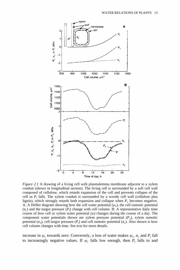
increase in ψc towards zero. Conversely, a loss of water makes ψc, πc and Pt fallto increasingly negative values. If ψc falls low enough, then Pt falls to and
Figure 2.1 A drawing of a living cell with plasmalemma membrane adjacent to a xylemconduit (shown in longitudinal section). The living cell is surrounded by a soft cell wallcomposed of cellulose, which retards expansion of the cell and prevents collapse of thecell as Pt falls. The xylem conduit is surrounded by a woody cell wall (cellulose pluslignin), which strongly retards both expansion and collapse when Px becomes negative.A: A Höfler diagram showing how the cell water potential (ψc), the cell osmotic potential(πc) and the turgor pressure (Pt) change with cell volume. B: A representative daily timecourse of how cell or xylem water potential (ψ) changes during the course of a day. Thecomponent water potentials shown are xylem pressure potential (Px), xylem osmoticpotential (πx), cell turgor pressure (Pt) and cell osmotic potential (πc). Also shown is howcell volume changes with time. See text for more details.
WATER RELATIONS OF PLANTS 13

remains at zero in cells in soft tissue. In woody tissues, i.e. in cells with lignifiedcell walls, the lignification will prevent cell collapse and Pt can fall to negativevalues. The information in the Höfler diagram can be used to understand thewater relations of cells in the course of a day.
A representative time course is shown in Figure 2.1B. Suppose the sun rises at06:00 and sets at 18:00. Radiant energy falling on leaves will enhance the rate ofevaporation above the rate at which roots can replace evaporated water, hence bothψc and ψx will fall to the most negative values in early afternoon (indicated bythe solid line marked by ψ in Figure 2.1B). As the afternoon progresses the lightintensity diminishes and the rate of water loss from the leaves falls below the rateof uptake of water from the roots; hence ψ increases. Overnight, the value of ψ willreturn to a value near zero in wet soils or more negative values in drier soils; ineither case ψ reaches a maximum value just prior to dawn. The value of ψ priorto sunrise (called the pre-dawn water potential) is often taken as a valid measureof soil dryness (=ψsoil) in the rooting zone of the plant. In the xylem, the osmoticpotential (πx) remains more or less constant and only slightly negative during theday. Therefore, all the change in ψx is brought about by a large change in Px,which closely parallels changes in ψ. Similarly, in living cells, changes in ψc arebrought about by large changes in Pt, while the cell osmotic potential (πc)changes only slightly and remains a large negative value.
WATER RELATIONS OF WHOLE PLANTS
The water relations of a whole plant can be understood in terms of thefundamental physiological role of the leaf. The leaf is an organ designed topermit CO2 uptake at a rate needed for photosynthesis while keeping waterevaporation from leaves to a reasonably low rate. The roots have the function ofextracting water from the soil to replace water evaporated from leaves.
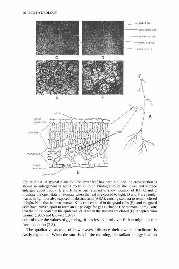
The leaf structure of a typical plant is illustrated in Figure 2.2. The upper andlower epidermis of leaves are covered with a waxy cuticle, which reduces waterloss from the leaf to negligible levels. All gas exchange into and out of the leaf isvia stomata. The guard cells of the stomata are capable of opening and closingair passages that provide pathways for diffusion of CO2 into the leaf and for lossof water vapour from the leaf. Photosynthesis occurs primarily in the palisadeand mesophyll cells of the leaf (Figure 2.2B). Leaves are thin enough (about 0.1mm thick) to permit photon penetration to chloroplasts (shown as dots inFigure 2.2B). The chloroplasts absorb the energy of the photon and, through aphotochemical process, use the energy to convert CO2 and water into sugar. Theconsumption of CO2 in the chloroplasts lowers the concentration of CO2 in thecells and thus sets up a concentration gradient for the diffusion of more CO2 intothe cells via the stomatal pores and mesophyll air spaces. Since mesophyll andpalisade cell surfaces are wet, water will evaporate continuously from thesesurfaces, and water vapour will diffuse continuously out of the leaf by the samepathway taken by CO2. Evaporated water is replaced continuously by water flow
14 ECO-HYDROLOGY
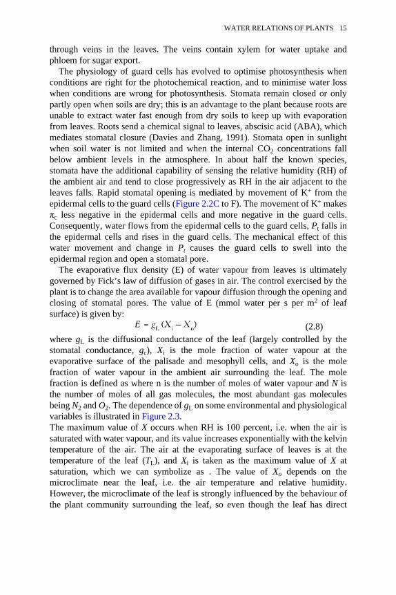
through veins in the leaves. The veins contain xylem for water uptake andphloem for sugar export.
The physiology of guard cells has evolved to optimise photosynthesis whenconditions are right for the photochemical reaction, and to minimise water losswhen conditions are wrong for photosynthesis. Stomata remain closed or onlypartly open when soils are dry; this is an advantage to the plant because roots areunable to extract water fast enough from dry soils to keep up with evaporationfrom leaves. Roots send a chemical signal to leaves, abscisic acid (ABA), whichmediates stomatal closure (Davies and Zhang, 1991). Stomata open in sunlightwhen soil water is not limited and when the internal CO2 concentrations fallbelow ambient levels in the atmosphere. In about half the known species,stomata have the additional capability of sensing the relative humidity (RH) ofthe ambient air and tend to close progressively as RH in the air adjacent to theleaves falls. Rapid stomatal opening is mediated by movement of K+ from theepidermal cells to the guard cells (Figure 2.2C to F). The movement of K+ makesπc less negative in the epidermal cells and more negative in the guard cells.Consequently, water flows from the epidermal cells to the guard cells, Pt falls inthe epidermal cells and rises in the guard cells. The mechanical effect of thiswater movement and change in Pt causes the guard cells to swell into theepidermal region and open a stomatal pore.
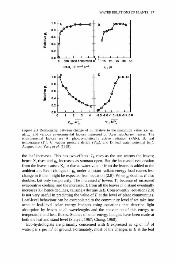
The evaporative flux density (E) of water vapour from leaves is ultimatelygoverned by Fick’s law of diffusion of gases in air. The control exercised by theplant is to change the area available for vapour diffusion through the opening andclosing of stomatal pores. The value of E (mmol water per s per m2 of leafsurface) is given by:
(2.8)where gL is the diffusional conductance of the leaf (largely controlled by thestomatal conductance, gc), Xi is the mole fraction of water vapour at theevaporative surface of the palisade and mesophyll cells, and Xo is the molefraction of water vapour in the ambient air surrounding the leaf. The molefraction is defined as where n is the number of moles of water vapour and N isthe number of moles of all gas molecules, the most abundant gas moleculesbeing N2 and O2. The dependence of gL on some environmental and physiologicalvariables is illustrated in Figure 2.3.The maximum value of X occurs when RH is 100 percent, i.e. when the air issaturated with water vapour, and its value increases exponentially with the kelvintemperature of the air. The air at the evaporating surface of leaves is at thetemperature of the leaf (TL), and Xi is taken as the maximum value of X atsaturation, which we can symbolize as . The value of Xo depends on themicroclimate near the leaf, i.e. the air temperature and relative humidity.However, the microclimate of the leaf is strongly influenced by the behaviour ofthe plant community surrounding the leaf, so even though the leaf has direct
WATER RELATIONS OF PLANTS 15
control over the values of gs and gL, it has less control over E than might appearfrom equation (2.8).
The qualitative aspects of how leaves influence their own microclimate iseasily explained. When the sun rises in the morning, the radiant energy load on
Figure 2.2 A: A typical plant. B: The lower leaf has been cut, and the cross-section isshown in enlargement at about 750×. C to F: Photographs of the lower leaf surfaceenlarged about 1000×. E and F have been stained to show location of K+. C and Eillustrate the open state of stomata when the leaf is exposed to light. D and F are similarleaves in light but also exposed to abscisic acid (ABA), causing stomata to remain closedin light. Note that in open stomata K+ is concentrated in the guard cells (E), and the guardcells have moved apart to form an air passage for gas exchange (the stomatal pore). Notethat the K+ is located in the epidermal cells when the stomata are closed (F). Adapted fromKramer (1983) and Bidwell (1979).
16 ECO-HYDROLOGY
the leaf increases. This has two effects. TL rises as the sun warms the leaves;hence Xi rises and gL increases as stomata open. But the increased evaporationfrom the leaves causes Xo to rise as water vapour from the leaves is added to theambient air. Even changes of gL under constant radiant energy load causes lesschange in E than might be expected from equation (2.8). When gt doubles E alsodoubles, but only temporarily. The increased E lowers TL because of increasedevaporative cooling, and the increased E from all the leaves in a stand eventuallyincreases X0; hence declines, causing a decline in E. Consequently, equation (2.8)is not very useful in predicting the value of E at the level of plant communities.Leaf-level behaviour can be extrapolated to the community level if we take intoaccount leaf-level solar energy budgets using equations that describe lightabsorption by leaves at all wavelengths and the conversion of this energy totemperature and heat fluxes. Studies of solar energy budgets have been made atboth the leaf and stand level (Slatyer, 1967; Chang, 1968).
Eco-hydrologists are primarily concerned with E expressed as kg or m3 ofwater per s per m2 of ground. Fortunately, most of the changes in E at the leaf
Figure 2.3 Relationship between change of gL relative to the maximum value, i.e. gL/gLmax, and various environmental factors measured on Acer saccharum leaves. Theenvironmental factors are A: photosynthetically active radiation (PAR); B: leaftemperature (TL); C: vapour pressure deficit (VPD); and D: leaf water potential (ψL).Adapted from Yang et al. (1998).
WATER RELATIONS OF PLANTS 17
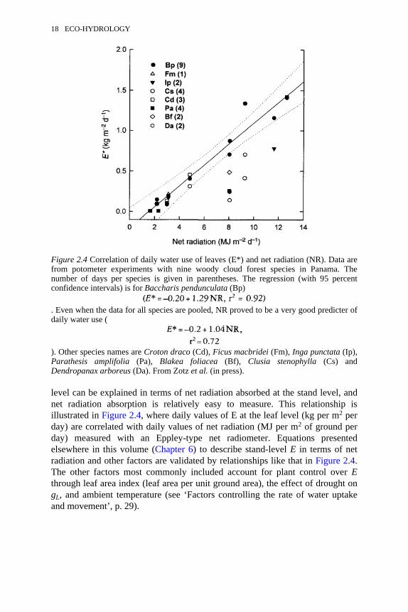
level can be explained in terms of net radiation absorbed at the stand level, andnet radiation absorption is relatively easy to measure. This relationship isillustrated in Figure 2.4, where daily values of E at the leaf level (kg per m2 perday) are correlated with daily values of net radiation (MJ per m2 of ground perday) measured with an Eppley-type net radiometer. Equations presentedelsewhere in this volume (Chapter 6) to describe stand-level E in terms of netradiation and other factors are validated by relationships like that in Figure 2.4.The other factors most commonly included account for plant control over Ethrough leaf area index (leaf area per unit ground area), the effect of drought ongL, and ambient temperature (see ‘Factors controlling the rate of water uptakeand movement’, p. 29).
Figure 2.4 Correlation of daily water use of leaves (E*) and net radiation (NR). Data arefrom potometer experiments with nine woody cloud forest species in Panama. Thenumber of days per species is given in parentheses. The regression (with 95 percentconfidence intervals) is for Baccharis pendunculata (Bp)
. Even when the data for all species are pooled, NR proved to be a very good predicter ofdaily water use (
). Other species names are Croton draco (Cd), Ficus macbridei (Fm), Inga punctata (Ip),Parathesis amplifolia (Pa), Blakea foliacea (Bf), Clusia stenophylla (Cs) andDendropanax arboreus (Da). From Zotz et al. (in press).
18 ECO-HYDROLOGY
WATER ABSORPTION BY PLANT ROOTS
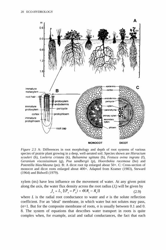
The primary factor affecting the pattern of water extraction by plants from soilsis the rooting depth. Rooting depths can be extremely variable, depending on soilconditions and species of plant producing the roots (Figure 2.5A). Many of theearly studies of rooting depth and the branching pattern of roots were performedin the 1920s and 1930s in deep, well-aerated prairie soils, where roots penetrateto great depths. At the extreme, roots have been traced to depths of 10 to 25 m,e.g. alfalfa (10 m), longleaf pine (17 m) (Kramer, 1983), and drought-evadingspecies in the California chaparral (25 m) (Stephen Davis, personalcommunication). The situation is very different for plants growing in heavysoils, where 90 percent of the roots can be found in the upper 0.5 to 1.0 m.
In seasonally dry regions, e.g. central Panama, the majority of the roots maybe located in the upper 0.5 m, but it is far from clear if the majority of waterabsorption occurs in the upper 0.5 m during the dry season. Water use by manyevergreen trees is higher in the dry season than in the wet season, even thoughthe upper 1 m of the soils has much lower potential than the leaves of the trees ( )(personal observation). Hence the role of shallow versus deep roots of woodyspecies deserves more study. In addition, deeply rooted species may contribute tothe water supply of shallow-rooted species through a process called ‘hydrauliclift’. In one study, it was found that shallow-rooted species growing within 1 to 5m of the base of maple trees were in a better water balance than the same speciesgrowing >5 m away (Dawson, 1993). Each night, ψsoil at a depth of 0.5 mincreased underneath maple trees but did not increase at distances >5 m from thetrees. This indicated that the deep maple roots were in contact with moist soil andwere capable of transporting water from deep roots to shallow roots overnight.Since the water potential of the shallow roots exceeded the water potential of theadjacent soil, water flow from the shallow roots to the adjacent soil contributedto the overnight rehydration of shallow soils. For more on hydraulic lift, seeRichards and Caldwell (1987) and Chapter 6.
Roots absorb both water and mineral solutes found in the soil, and the flows ofsolutes and water interact with each other. The mechanism and pathway of waterabsorption by roots is more complex than in the case of a single cell (see above).Water must first travel radially from the epidermis to cortex, endodermis andpericycle before it finally reaches the xylem vessels, from which point water flowis axial along the root (Figure 2.5B and C). The radial pathway (typically 0.3 mmlong in young roots) is usually much less conductive than the axial pathway (>1m in many cases); hence whole-root conductance is generally proportional to theroot surface area. The radial pathway can be viewed as a ‘composite membrane’separating the soil solution from the solution in the xylem fluid. The compositemembrane consists of serial and parallel pathways made up of plasmalemmamembranes, cell wall ‘membranes’ and plasmodesmata (pores <0.5 µmdiameter) that connect adjacent cells. The composite membrane is rather leaky tosolutes; hence differences in osmotic potential between the soil (πs) and the
WATER RELATIONS OF PLANTS 19
xylem (πx) have less influence on the movement of water. At any given pointalong the axis, the water flux density across the root radius (Jt) will be given by
(2.9)where L is the radial root conductance to water and σ is the solute reflectioncoefficient. For an ‘ideal’ membrane, in which water but not solutes may pass,(σ=1. But for the composite membrane of roots, σ is usually between 0.1 and 0.8. The system of equations that describes water transport in roots is quitecomplex when, for example, axial and radial conductances, the fact that each
Figure 2.5 A: Differences in root morphology and depth of root systems of variousspecies of prairie plant growing in a deep, well-aerated soil. Species shown are Hieraciumscouleri (h), Loeleria cristata (k), Balsamina sgittata (b), Festuca ovina ingrata (f),Geranium viscosissimum (g), Poa sandbergii (p), Hoorebekia racemosa (ho) andPotentilla blaschkeana (po). B: A dicot root tip enlarged about 50×. C: Cross-section ofmonocot and dicot roots enlarged about 400×. Adapted from Kramer (1983), Steward(1964) and Bidwell (1979).
20 ECO-HYDROLOGY
solute has a different σ, and the influence of solute loading rate (Js) on water floware taken into account. Water and solute flow in roots can be described by astanding gradient osmotic flow model, and readers interested in the details mayconsult Tyree et al. (1994b) and Steudle (1992).
Fortunately, the equations describing water flow become quite simple whenthe rate of water flow is high. The concentration of solutes in the xylem fluid isdetermined by the ratio of solute flux to water flux (Js/Jw). Solute flux tends to bemore or less constant with time, but water flux increases with increasingtranspiration. When water flow is high, the concentration of solutes in the xylemfluid becomes quite small and approaches values comparable with that in the soilsolution, and pressure differences become quite large, hence . Only at night orduring rainy periods can values of approach those of . So water flow through awhole root system during the day can be approximated by
(2.10)where Px, b is the xylem pressure at the base of the plant and Kr is the total rootconductance (combined radial and axial conductances).
THE PATHWAY OF WATER MOVEMENT (HYDRAULICARCHITECTURE)
Van den Honert (1948) quantified water flow in plants in a classical paper inwhich he viewed the flow of water in the plant as a catenary process, where eachcatena element is viewed as a hydraulic conductance (analogous to an electricalconductance) across which water (analogous to electrical current) flows. Thus,van den Honert proposed an Ohm’s law analogue for water flow in plants. TheOhm’s law analogue leads to the following predictions: (1) the driving force ofsap ascent is a continuous decrease in Px in the direction of sap flow; and (2)evaporative flux density from leaves (E) is proportional to the negative of thepressure gradient (−dPx/dx) at any given ‘point’ (cross-section) along thetranspiration stream. Thus at any given point of a root, stem or leaf vein wehave:
(2.11)where A is leaf area supplied by a stem segment with hydraulic conductivity Kh,and ρg dh/dx is the gravitational potential gradient, where ρ is the density ofwater, g is acceleration due to gravity, and h is vertical distance and x actualdistance travelled by water in the stem segment.
In the context of stem segments of length (L) with finite pressure drops acrossends of the segment we have:
(2.12)Figure 2.6 illustrates water flow through a plant represented by a linear catena ofconductance elements near the centre and a branched catena of conductanceelements on the left. The number and arrangement of catena elements is dictated
WATER RELATIONS OF PLANTS 21
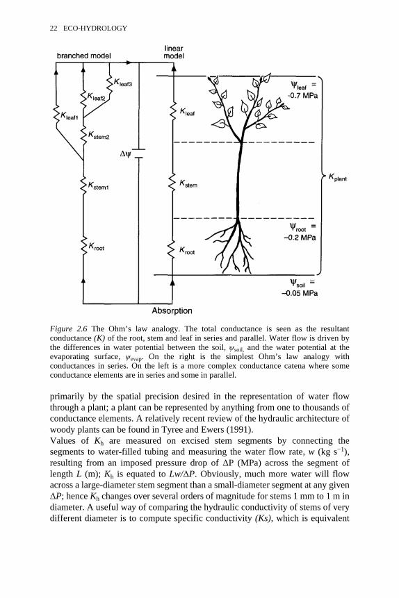
primarily by the spatial precision desired in the representation of water flowthrough a plant; a plant can be represented by anything from one to thousands ofconductance elements. A relatively recent review of the hydraulic architecture ofwoody plants can be found in Tyree and Ewers (1991). Values of Kh are measured on excised stem segments by connecting thesegments to water-filled tubing and measuring the water flow rate, w (kg s−1),resulting from an imposed pressure drop of ∆P (MPa) across the segment oflength L (m); Kh is equated to Lw/∆P. Obviously, much more water will flowacross a large-diameter stem segment than a small-diameter segment at any given∆P; hence Kh changes over several orders of magnitude for stems 1 mm to 1 m indiameter. A useful way of comparing the hydraulic conductivity of stems of verydifferent diameter is to compute specific conductivity (Ks), which is equivalent
Figure 2.6 The Ohm’s law analogy. The total conductance is seen as the resultantconductance (K) of the root, stem and leaf in series and parallel. Water flow is driven bythe differences in water potential between the soil, ψsoil, and the water potential at theevaporating surface, ψevap. On the right is the simplest Ohm’s law analogy withconductances in series. On the left is a more complex conductance catena where someconductance elements are in series and some in parallel.
22 ECO-HYDROLOGY
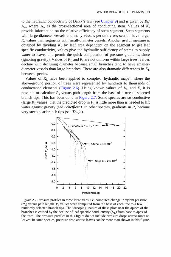
to the hydraulic conductivity of Darcy’s law (see Chapter 9) and is given by Kh/Aw, where Aw is the cross-sectional area of conducting stem. Values of Ksprovide information on the relative efficiency of stem segment. Stem segmentswith large-diameter vessels and many vessels per unit cross-section have largerKs values than segments with small-diameter vessels. Another useful measure isobtained by dividing Kh by leaf area dependent on the segment to get leafspecific conductivity, values give the hydraulic sufficiency of stems to supplywater to leaves and permit the quick computation of pressure gradients, since(ignoring gravity). Values of KL and Ks are not uniform within large trees; valuesdecline with declining diameter because small branches tend to have smaller-diameter vessels than large branches. There are also dramatic differences in KLbetween species.
Values of KL have been applied to complex ‘hydraulic maps’, where theabove-ground portion of trees were represented by hundreds to thousands ofconductance elements (Figure 2.6). Using known values of KL and E, it ispossible to calculate Px versus path length from the base of a tree to selectedbranch tips. This has been done in Figure 2.7. Some species are so conductive(large KL values) that the predicted drop in Px is little more than is needed to liftwater against gravity (see Schefflera). In other species, gradients in Px becomevery steep near branch tips (see Thuja).
Figure 2.7 Pressure profiles in three large trees, i.e. computed change in xylem pressure(Px) versus path length. Px values were computed from the base of each tree to a fewrandomly selected branch tips. The ‘drooping’ nature of these plots near the apices of thebranches is caused by the decline of leaf specific conductivity (KL) from base to apex ofthe trees. The pressure profiles in this figure do not include pressure drops across roots orleaves. In some species, pressure drop across leaves can be more than shown in this figure.
WATER RELATIONS OF PLANTS 23
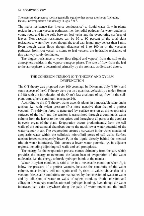
The pressure drop across roots is generally equal to that across the shoots (includingleaves). E=evaporative flux density in kg s−1 m−2.
The major resistance (i.e. inverse conductance) to liquid water flow in plantsresides in the non-vascular pathways, i.e. the radial pathway for water uptake inyoung roots and in the cells between leaf veins and the evaporating surfaces ofleaves. Non-vascular resistances can be 60 to 90 percent of the total plantresistance to water flow, even though the total path length may be less than 1 mm.Even though water flows though distances of 1 to 100 m in the vascularpathways from root vessel to stems to leaf vessels, the hydraulic resistance ofthis pathway rarely dominates.
The biggest resistance to water flow (liquid and vapour) from the soil to theatmosphere resides in the vapour transport phase. The rate of flow from the leafto the atmosphere is determined primarily by the stomata, as discussed above.
THE COHESION-TENSION (C-T) THEORY AND XYLEMDYSFUNCTION
The C-T theory was proposed over 100 years ago by Dixon and Joly (1894), andsome aspects of the C-T theory were put on a quantitative basis by van den Honert(1948) with the introduction of the Ohm’s law analogue of sap flow in the soil-plant-atmosphere continuum (see page 24).
According to the C-T theory, water ascends plants in a metastable state undertension, i.e. with xylem pressure (Px) more negative than that of a perfectvacuum. The driving force is generated by surface tension at the evaporatingsurfaces of the leaf, and the tension is transmitted through a continuous watercolumn from the leaves to the root apices and throughout all parts of the apoplastin every organ of the plant. Evaporation occurs predominantly from the cellwalls of the substomatal chambers due to the much lower water potential of thewater vapour in air. The evaporation creates a curvature in the water menisci ofapoplastic water within the cellulosic microfibril pores of cell walls. Surfacetension forces consequently lower Px in the liquid directly behind the menisci(the air-water interfaces). This creates a lower water potential, ψ, in adjacentregions, including adjoining cell walls and cell protoplasts.
The energy for the evaporation process comes ultimately from the sun, whichprovides the energy to overcome the latent heat of evaporation of the watermolecules, i.e. the energy to break hydrogen bonds at the menisci.
Water in xylem conduits is said to be in a metastable condition when Px isbelow the pressure of a perfect vacuum, because the continuity of the watercolumn, once broken, will not rejoin until Px rises to values above that of avacuum. Metastable conditions are maintained by the cohesion of water to waterand by adhesion of water to walls of xylem conduits. Both cohesion andadhesion of water are manifestations of hydrogen bonding. Even though air-waterinterfaces can exist anywhere along the path of water movement, the small
24 ECO-HYDROLOGY
diameter of pores in cell walls and the capillary forces produced by surfacetension within such pores prevent the passage of air into conduits under normalcircumstances. However, when Px becomes sufficiently negative, air bubbles canbe sucked into xylem conduits through porous walls.
This tension (negative Px) is ultimately transferred to the roots, where itlowers ψ of the roots below the ψ of the soil water. This causes water uptakefrom the soil to the roots and from the roots to the leaves to replace waterevaporated at the surface of the leaves. The Scholander-Hammel pressure bomb(Scholander et al., 1965) is one of the most frequently used tools for estimatingPx. Typically, Px can range down to −2 MPa (in crop plants) or to −4 MPa (inarid zone species) and in some cases −10 MPa (in California chaparral species).Readers interested in learning more about the cohesion-tension theory of sapascent may refer to Tyree (in press).
In some plants, water movement can occur at night or during rain events, whenPx is positive due to root pressure, i.e. osmotically driven flow from roots. Waterflow under positive Px is often accompanied by gutation, i.e. the formation ofwater droplets at leaf margins. But water is normally under negative pressure(tension) as it moves through the xylem towards the leaves during sunny days.The water is thus in a metastable condition and vulnerable to cavitation due to airentry into the water columns. Cavitation results in embolism (air blockage), thusdisrupting the flow of water (Tyree and Sperry, 1989). Cavitation in plants canresult from water stress, and each species has a characteristic ‘vulnerabilitycurve’, which is a plot of the percentage loss of Kh in stems versus the xylempressure potential, Px, required to induce the loss. Vulnerability curves aretypically measured by dehydrating large excised branches to known Px. Stemsegments are then cut under water from the dehydrated branches and, for themost part, the air bubbles remain inside the conduits. An initial conductivitymeasurement is made and compared with the maximum Kh after air bubbles havebeen dissolved. The vulnerability curves of plants, in concert with their hydraulicarchitecture, can give considerable insight into drought tolerance and waterrelations ‘strategies’.
The vulnerability curves for a number of species are reproduced in Figure 2.8(Tyree et al. 1994a). These species represent the range of vulnerabilitiesobserved so far in over sixty species; 50 percent loss of Kh occurs at Px valuesranging from −0.7 to −11 MPa. Many plants growing in areas with seasonalrainfall patterns (wet and dry periods) appear to be drought evaders, while othersare drought toleraters. The drought evaders avoid drought (low Px and highpercentage loss Kh) by having deep roots and a highly conductive hydraulicsystem. Alternatively, they evade drought by being deciduous. The other speciesfrequently reach very negative Px for part or all of the year and are shallow-rooted or grow in saline environments. These species survive by having avascular system highly resistant to cavitations. Embolisms may be dissolved in plants if Px in the xylem becomes positive or closeto positive for adequate time periods (Tyree and Yang, 1992; Lewis et al., 1994).
WATER RELATIONS OF PLANTS 25
Embolisms disappear by dissolution of air into the water surrounding the airbubble. The solubility of air in water is proportional to the pressure of airadjacent to the water (Henry’s law). Water in plants tends to be saturated with airat a concentration determined by the average atmospheric pressure of gassurrounding plants. Thus, for air to dissolve from a bubble into water, the air inthe bubble has to be at a pressure in excess of atmospheric pressure. If thepressure of water (Px) surrounding a bubble is equal to atmospheric pressure (Pa),bubbles will naturally dissolve, because surface tension (τ) of water raises thepressure of air in the bubble (Pb) above Pa. In general, where r is the radius of thebubble. According to the cohesion theory of sap ascent, Px is drawn below Paduring transpiration. Since 2T/r of a dissolving bubble in a vessel is usually <0.03 MPa, and since Px is in the range of−0.1 to −10 MPa during transpiration, Pbis usually ≤Pa, and hence bubbles, once formed in vessels, rarely completelydissolve. Repair (i.e. dissolution) occurs only when Px becomes large via rootpressure. One notable exception to this generality has recently been found inLaurus nobilis shrubs, which appear to be able to refill embolised vessels evenwhile Px is at −1 MPa (Salleo et al., 1996). The mechanism involved has evadedexplanation.
Figure 2.8 Vulnerability curves for various species, y-axis is percentage loss of hydraulicconductivity induced by the xylem pressure potential, Px, shown on the x-axis. C =Ceanothus megacarpus, J = Juniperus virginiana, R = Rhizophora mangle, A = Acersaccharum, T = Thuja occidentalis, P = Populus deltoides.
26 ECO-HYDROLOGY

WATER RELATIONS OF PLANTS FACTORSCONTROLLING THE RATE OF WATER UPTAKE AND
MOVEMENT
Environmental conditions control the rate of water movement in plants. Thedominant environmental factor is net solar radiation, as mentioned previously.Water movement can be explained by the solar energy budget of plants. We willnow take a more quantitative look at the solar energy budget of plants at both theleaf and stand level.
Leaf-level energy budgets
Objects deep in space far away from solar radiation tend to be rather cold (about5 K), whereas objects on Earth tend to be rather warm (270–310 K). The reasonfor the elevated temperature on Earth is the warming effect of solar radiation.The net radiation absorbed by a leaf (RNL, W m−2) can be arbitrarily divided intoshort-wave and long-wave radiation, with the demarcation wavelength being at 1µm. Most short-wave radiation comes from the Sun, and most long-waveradiation comes from the Earth. As a leaf absorbs RNL, the leaf temperature (TL)rises, which increases the loss of energy from the leaf by three differentmechanisms—black body radiation (B), sensible heat flux (H), and latent heat ofvaporisation of water (AE, where E is the evaporative flux density of water dueto transpiration (mol of water s−1 m−2) and λ is the heat required to evaporate amole of water (J mol−1)). RNL can also be converted to chemical energy by theprocess of photosynthesis and to energy storage, but these two factors aregenerally small for leaves and are ignored in the equation below:
(2.13)The B in equation (2.13) is the ‘black body’ radiation. All objects emit radiation.Very hot objects like the Sun emit mostly short-wave radiation, whereas coolerobjects on Earth emit mostly long-wave radiation. The amount of radiationemitted increases with the kelvin temperature according to the Stefan-Boltzmannlaw: i.e. where e is the emissivity (≥0.95 for leaves), and σsb is the Stefan-Boltzmann constant= H in equation (2.13) is sensible heat flux density, i.e. theheat transfer by heat diffusion between objects at different temperatures. Forleaves, the heat transfer is between the leaf and the surrounding air. The rate ofheat transfer is proportional to the difference in temperature between the leaf andthe air, so where Ta is the air temperature and k is the heat transfer coefficient.Heat transfer is more rapid and hence k is larger under windy conditions than instill air. But the value of k is also determined by leaf size, shape and orientationwith respect to the wind direction. Readers interested in more detail shouldconsult Slatyer (1967) or Nobel (1991).
The factors determining E have already been given in equation (2.8), so if wecombine equation (2.8) with the other equations for B and H we get:
WATER RELATIONS OF PLANTS 27
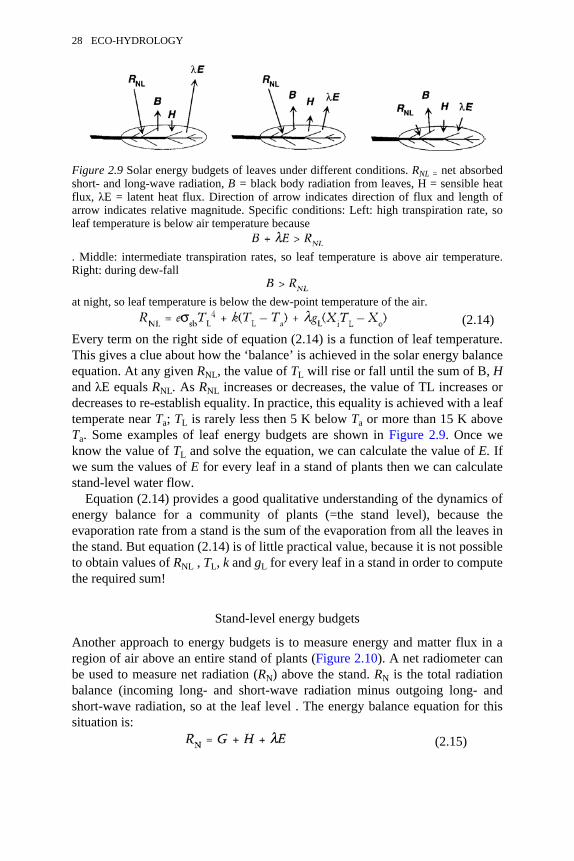
(2.14)Every term on the right side of equation (2.14) is a function of leaf temperature.This gives a clue about how the ‘balance’ is achieved in the solar energy balanceequation. At any given RNL, the value of TL will rise or fall until the sum of B, Hand λE equals RNL. As RNL increases or decreases, the value of TL increases ordecreases to re-establish equality. In practice, this equality is achieved with a leaftemperate near Ta; TL is rarely less then 5 K below Ta or more than 15 K aboveTa. Some examples of leaf energy budgets are shown in Figure 2.9. Once weknow the value of TL and solve the equation, we can calculate the value of E. Ifwe sum the values of E for every leaf in a stand of plants then we can calculatestand-level water flow.
Equation (2.14) provides a good qualitative understanding of the dynamics ofenergy balance for a community of plants (=the stand level), because theevaporation rate from a stand is the sum of the evaporation from all the leaves inthe stand. But equation (2.14) is of little practical value, because it is not possibleto obtain values of RNL , TL, k and gL for every leaf in a stand in order to computethe required sum!
Stand-level energy budgets
Another approach to energy budgets is to measure energy and matter flux in aregion of air above an entire stand of plants (Figure 2.10). A net radiometer canbe used to measure net radiation (RN) above the stand. RN is the total radiationbalance (incoming long- and short-wave radiation minus outgoing long- andshort-wave radiation, so at the leaf level . The energy balance equation for thissituation is:
(2.15)
Figure 2.9 Solar energy budgets of leaves under different conditions. RNL = net absorbedshort- and long-wave radiation, B = black body radiation from leaves, H = sensible heatflux, λE = latent heat flux. Direction of arrow indicates direction of flux and length ofarrow indicates relative magnitude. Specific conditions: Left: high transpiration rate, soleaf temperature is below air temperature because
. Middle: intermediate transpiration rates, so leaf temperature is above air temperature.Right: during dew-fall
at night, so leaf temperature is below the dew-point temperature of the air.
28 ECO-HYDROLOGY

The rate of heat storage in the soil, G (W m−2), can be significant, because soiltemperature can change by a few K on a daily basis in the upper few centimetresof soil. Heat storage rate is usually measured with a soil heat flux sensor. The Hand λE terms are similar to those in equation (2.14), but the equations define theflux densities between the heights marked ‘*’ and ‘**’ in Figure 2.10. The fluxof heat and water vapour across the distance ∆Z is controlled by vertical airconvection (eddy), and the defining equations are:
(2.16)and
(2.17)
where Ke is the eddy transfer coefficient, Cp is the heat capacity of air, pa is theair density, ∆T is the difference in air temperature measured at the two levels inFigure 2.10 separated by a height difference of ∆Z, and A[H2O] is the differencein water vapour concentration at the two levels in Figure 2.10 separated by aheight difference of ∆Z.
It is easy to measure AT and A[H2O] but difficult to assign a value for Ke,which changes dynamically with changes in wind velocity, so the usual practice
Figure 2.10 Solar energy budget of a uniform stand of plants. Net radiation (RN) ismeasured at location marked ‘*’, air temperature and relative humidity is measured atlocations marked ‘*’ and ‘**’. Rate of heat storage in soil is measured at ‘***’.
WATER RELATIONS OF PLANTS 29
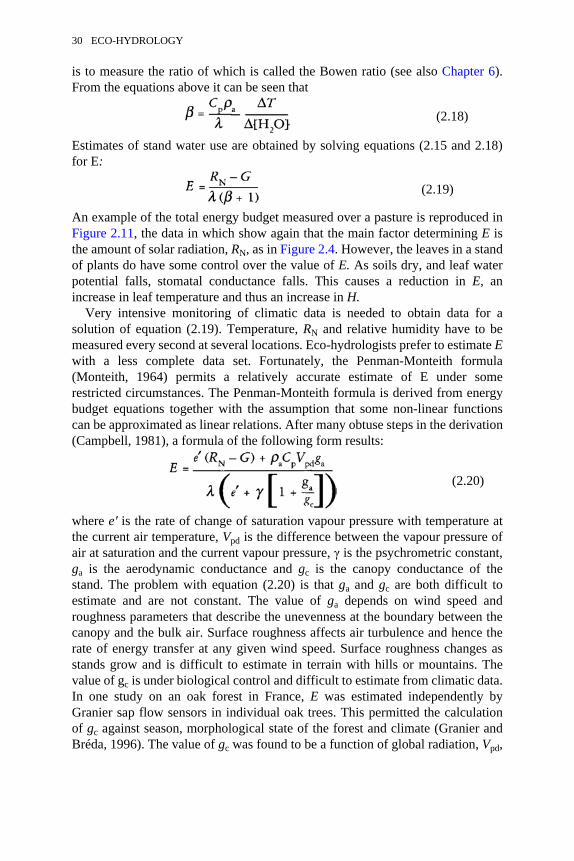
is to measure the ratio of which is called the Bowen ratio (see also Chapter 6).From the equations above it can be seen that
(2.18)
Estimates of stand water use are obtained by solving equations (2.15 and 2.18)for E:
(2.19)
An example of the total energy budget measured over a pasture is reproduced inFigure 2.11, the data in which show again that the main factor determining E isthe amount of solar radiation, RN, as in Figure 2.4. However, the leaves in a standof plants do have some control over the value of E. As soils dry, and leaf waterpotential falls, stomatal conductance falls. This causes a reduction in E, anincrease in leaf temperature and thus an increase in H.
Very intensive monitoring of climatic data is needed to obtain data for asolution of equation (2.19). Temperature, RN and relative humidity have to bemeasured every second at several locations. Eco-hydrologists prefer to estimate Ewith a less complete data set. Fortunately, the Penman-Monteith formula(Monteith, 1964) permits a relatively accurate estimate of E under somerestricted circumstances. The Penman-Monteith formula is derived from energybudget equations together with the assumption that some non-linear functionscan be approximated as linear relations. After many obtuse steps in the derivation(Campbell, 1981), a formula of the following form results:
(2.20)
where e′ is the rate of change of saturation vapour pressure with temperature atthe current air temperature, Vpd is the difference between the vapour pressure ofair at saturation and the current vapour pressure, γ is the psychrometric constant,ga is the aerodynamic conductance and gc is the canopy conductance of thestand. The problem with equation (2.20) is that ga and gc are both difficult toestimate and are not constant. The value of ga depends on wind speed androughness parameters that describe the unevenness at the boundary between thecanopy and the bulk air. Surface roughness affects air turbulence and hence therate of energy transfer at any given wind speed. Surface roughness changes asstands grow and is difficult to estimate in terrain with hills or mountains. Thevalue of gc is under biological control and difficult to estimate from climatic data.In one study on an oak forest in France, E was estimated independently byGranier sap flow sensors in individual oak trees. This permitted the calculationof gc against season, morphological state of the forest and climate (Granier andBréda, 1996). The value of gc was found to be a function of global radiation, Vpd,
30 ECO-HYDROLOGY
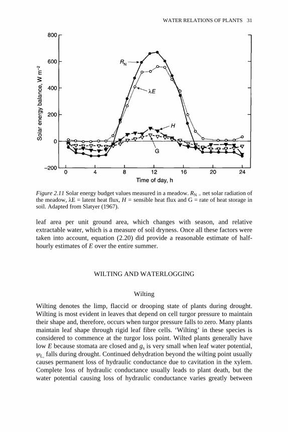
leaf area per unit ground area, which changes with season, and relativeextractable water, which is a measure of soil dryness. Once all these factors weretaken into account, equation (2.20) did provide a reasonable estimate of half-hourly estimates of E over the entire summer.
WILTING AND WATERLOGGING
Wilting
Wilting denotes the limp, flaccid or drooping state of plants during drought.Wilting is most evident in leaves that depend on cell turgor pressure to maintaintheir shape and, therefore, occurs when turgor pressure falls to zero. Many plantsmaintain leaf shape through rigid leaf fibre cells. ‘Wilting’ in these species isconsidered to commence at the turgor loss point. Wilted plants generally havelow E because stomata are closed and gs is very small when leaf water potential,ψL, falls during drought. Continued dehydration beyond the wilting point usuallycauses permanent loss of hydraulic conductance due to cavitation in the xylem.Complete loss of hydraulic conductance usually leads to plant death, but thewater potential causing loss of hydraulic conductance varies greatly between
Figure 2.11 Solar energy budget values measured in a meadow. RN = net solar radiation ofthe meadow, λE = latent heat flux, H = sensible heat flux and G = rate of heat storage insoil. Adapted from Slatyer (1967).
WATER RELATIONS OF PLANTS 31

species (see Figure 2.8). Some plants in arid environments avoid drought eitherby having short reproductive cycles confined to brief wet periods or by havingdeep roots that can access deep sources of soil water (Kramer, 1983).
As plants approach the wilting point, there is a gradual loss in stomatalconductance and, hence, a reduction in E and photosynthetic rate (Schulze andHall, 1982). Some species are much more sensitive than others (Figure 2.12B). Theshort-term effects of decreased ψL on transpiration are less dramatic than arelong-term effects (Figure 2.12A). Long-term effects of drought are mediated byhormone signals from roots, which cause a medium-term decline in gs and bychanges in root morphology, e.g. loss of fine roots, suberisation of root surfaces,and formation of corky layers (Ginter-Whitehouse et al., 1983). Themorphological changes to roots cause an decrease in whole plant hydraulicconductance (KD), so ψL becomes more negative at lower values of E because .Very severe drought can further lower Kp due to cavitation of xylem vessels.
Waterlogging
Waterlogging denotes an environmental condition of soil water saturation orponding of water, which can last for a just a few hours or for many months.Plants absent from flood-prone sites are damaged easily by waterlogging. On theother hand, plants that inhabit flood-prone sites include species that can growactively in flooded soils or species that survive flooding in a quiescent ordormant state (see Chapter 5). Paradoxically, the commonest sign of tobaccoroots having an excess of water is the development of a water deficit in theleaves (Kramer, 1983; Kramer and Jackson, 1954); but flood-tolerant species arenot so easily affected.
Flooding often affects root morphology and physiology. The wilting anddefoliation that is found on flooding can be traced to an increased resistance towater flux in the roots (Mees and Weatherley, 1957). In most flood-tolerantspecies, flooding induces morphological changes in the roots. Thesemodifications usually involve root thickening, with an increase in porosity. Theincrease in porosity increases the rate of oxygen diffusion to root tips and thuspermits continued aerobic metabolism in the inundated roots. In flood-sensitivespecies, root and shoot growth are rapidly reduced on flooding, and root tips maybe damaged. Growth of roots can be renewed only from regions proximal to thestem. The physiological responses and adaptations to waterlogging are numerousand beyond the scope of this chapter, but interested readers may get into theliterature by consulting Crawford (1982).
CONCLUSION
Water flow through plants is purely passive. Water flow through most of theplant is driven by differences in water pressure, ∆P. According to the cohesion-tension theory of sap ascent, water movement is driven by surface tension effects
32 ECO-HYDROLOGY
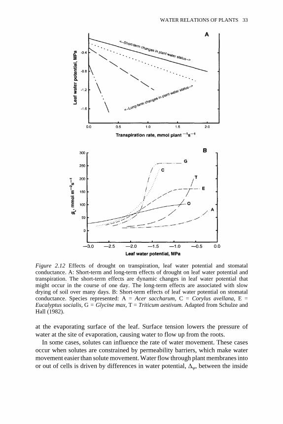
at the evaporating surface of the leaf. Surface tension lowers the pressure ofwater at the site of evaporation, causing water to flow up from the roots.
In some cases, solutes can influence the rate of water movement. These casesoccur when solutes are constrained by permeability barriers, which make watermovement easier than solute movement. Water flow through plant membranes intoor out of cells is driven by differences in water potential, ∆ψ, between the inside
Figure 2.12 Effects of drought on transpiration, leaf water potential and stomatalconductance. A: Short-term and long-term effects of drought on leaf water potential andtranspiration. The short-term effects are dynamic changes in leaf water potential thatmight occur in the course of one day. The long-term effects are associated with slowdrying of soil over many days. B: Short-term effects of leaf water potential on stomatalconductance. Species represented: A = Acer saccharum, C = Corylus avellana, E =Eucalyptus socialis, G = Glycine max, T = Triticum aestivum. Adapted from Schulze andHall (1982).
WATER RELATIONS OF PLANTS 33
and outside of the cell. Differences in ψ are determined by differences inpressure and solute potential − ∆P and ∆πT, respectively. Water flow throughroots is driven by ∆P and more weakly by ∆π, because roots are leaky to solutes.Water flow rates through roots are usually high enough to make ∆π much lessthan ∆P, so most of the time water flow through roots is driven by the pressuredifference between the water in the soil and the base of the plant.
The rate of evaporation of water from plants is controlled by both the plantand the environment. The plant controls water movement via the stomatalphysiology. Stomata respond to changes in light, temperature, CO2, leaf waterpotential and humidity by increasing or decreasing leaf conductance (gL) towater vapour diffusion. The most important environmental factor controllingevaporation is then net radiation absorbed by plants.
REFERENCES
Bidwell, R.G.S. (1979) Plant Physiology, New York: Macmillan.Campbell, G.S. (1981) Fundamentals of radiation and temperature relations, Encyclopedia
of Plant Physiology, New Series Vol. 12A: 11–40, New York: Springer-Verlag.Chang, J.-H. (1968) Climate and Agriculture, Chicago: Aldine Publishing Co.Crawford, R.M.M. (1982) Physiological responses to flooding. Encyclopedia of Plant
Physiology, New Series Vol. 12B: 453–477, New York: Springer-Verlag.Davies, W.J. and Zhang, J. (1991) Root signals and the regulation of growth
and development of plants in drying soil, Annual Review of Plant Physiology andPlant Molecular Biology 42:55–76.
Dawson, T.E. (1993) Hydraulic lift and water parasitism by plants: implications for waterbalance, performance, and plant-plant interactions, Oecologia 95:565–574.
Dixon, H.H. and Joly, J. (1894) On the ascent of sap, Philosophical Transactions of theRoyal Society, London, Series B, 186:563–576.
Ginter-Whitehouse, D.L., Hinckley, T.M. and Pallardy, S.G. (1983) Spatial and temporalaspects of water relations of three tree species with different vascular anatomy,Forest Science 29:317–329.
Granier, A. and Bréda, N. (1996) Modelling canopy conductance and stand transpirationof an oak forest from sap flow measurements, Annales des Sciences Forestières 53:537–546.
Kramer, P.J. (1983) Water Relations of Plants, New York: Academic Press.Kramer, P.J. and Jackson, W.T. (1954) Causes of injury to flooded tobacco plants, Plant
Physiology 29:241–245.Lewis, A.M., Harnden, V.D. and Tyree, M.T. (1994) Collapse of water-stress emboli in
the tracheids of Thuja occidentalis L., Plant Physiology 106:1639–1646.Mees, G.C. and Weatherley, P.E. (1957) The mechanism of water absorption by roots. II.
The role of hydrostatic pressure gradients. Proceedings of the Royal Society,London, Series B, 147:381–391.
Monteith, J.L. (1964) Evaporation and environment, Symposium of the Society forExperimental Biology 19:205–234.
Nobel, P.S. (1991) Physiochemical and Environmental Plant Physiology, New York:Academic Press.
34 ECO-HYDROLOGY
Richards, J.R. and Caldwell, M.M. (1987) Hydraulic lift: substantial nocturnal watertransport between soil layers by Artemisia tridentata roots, Oecologia 74: 486–489.
Salleo, S., LoGullo, M.A., De Paoli, D. and Zippo, M. (1996) Xylem recovery fromcavitation-induced embolism in young plants of Laurus nobilis: a possiblemechanism, New Phytologist 132:47–56.
Scholander, P.F., Hammel, H.T., Bradstreet, E.D. and Hemmingsen, E.A. (1965) Sappressure in vascular plants, Science 148:339–346.
Slatyer, R.O. (1967) Plant Water Relationships, New York: Academic Press.Schulze, E.D. and Hall, A.E. (1982) Stomatal responses, water loss and CO2 assimilation
rates of plants in contrasting environments. Encyclopedia of Plant Physiology, NewSeries Vol. 12B: 181–230.
Steudle, E. (1992) The biophysics of plant water: Compartmentation, coupling withmetabolic processes, and flow of water in plant roots, in Somero, G.N.Osmond, C.B.and Bolis, C.L. (eds) Water and Life; Comparative Analysis of Water Relationshipsat the Organismic, Cellular, and Molecular Levels, Heidelberg: Springer-Verlag,pp. 173–204.
Steward, F.C. (1964) Plants at Work, Reading, Mass.: Addison-Wesley. Tyree, M.T. (inpress) The cohesion-tension theory of sap ascent: current controversies, Journal ofExperimental Botany.
Tyree, M.T. and Ewers, F.W. (1991) The hydraulic architecture of trees and other woodyplants, New Phytologist 119:345–360.
Tyree, M.T. and Sperry, J.S. (1989) The vulnerability of xylem to cavitation andembolism, Annual Review of Plant Physiology and Molecular Biology 40:19–38.
Tyree, M.T. and Yang, S. (1992) Hydraulic conductivity recovery versus water pressurein xylem of Acer saccharum, Plant Physiology 100:669–676.
Tyree, M.T., Davis, S.D. and Cochard, H. (1994a) Biophysical perspectives of xylemevolution: is there a trade off of hydraulic efficiency for vulnerability to dysfunction?Journal of the International Association of Wood Anatomists 15: 335–360.
Tyree, M.T., Cruiziat, P. and Sinclair, B. (1994b) Novel methods of measuring hydraulicconductivity of tree root systems and interpretation using AMAIZED: A maize-rootdynamic model for water and solute transport, Plant Physiology 104: 189–199.
van den Honert, T.H. (1948) Water transport in plants as a catenary process, Discussionsof the Faraday Society 3:146–153.
Yang, S., Liu, X. and Tyree, M.T. (in press) A model of stomatal conductance in sugarmaple (Acer saccharum Marsh) , Journal of Theoretical Biology.
Zotz, G., Tyree, M.T., Patino, S. and Carlton, M.R. (1998) Hydraulic architecture andwater use of selected species from a lower montane forest in Panama. Trees 12:302–309.
WATER RELATIONS OF PLANTS 35
3SCALES OF INTERACTION IN ECO-
HYDROLOGICAL RELATIONSRobert L.Wilby and David S.Schimel
INTRODUCTION
parameters and processes important at one scale are frequently notimportant or predictive at another scale, and information is often lostas spatial [or temporal] data are considered at coarser scales ofresolution.
Turner, M.G. (1990)
This observation holds for all the geophysical and biological sciences, includingeco-hydrology. Indeed, ‘scale issues’ have become the legitimate focus of agrowing body of research in the environmental sciences and were even identifiedas a research priority by the US Committee on Opportunities in the HydrologicalSciences (James, 1995). According to Blöschl and Sivapalan (1995), the task oflinking and integrating hydrological ‘laws’ at different scales has not yet beenfully addressed, and doing so remains an outstanding challenge in the field ofsurficial processes. Several factors have contributed to the current awareness ofscale issues in plant-water relations.First, recent population growth, technological developments and economicactivities have broadened the scale of human interference in hydrosystems.Historically, the hydrological discipline evolved from the technical demands ofsupplying societies with potable water for domestic and agriculturalconsumption, disposing of liquid wastes, and protecting land from inundations(Klemes, 1988; Wilby, 1997a). Such concerns were initially small-scale but havenow attained global dimensions with respect to climate change impacts, regionalland-use changes, and the potential for transboundary pollution incidents.
Second, most meteorological, hydrological and ecological processes arestrongly heterogeneous in both space and time. However, our ability to observeand/or sample these processes is severely constrained by theavailable technology, human and financial resources, and a general lack ofstandardisation in measurement techniques (Rodda, 1995). At the same time,
modelling often demands long-term, spatially consistent descriptions ofheterogeneous parameters such as albedo or soil hydraulic characteristics. Aswill be shown below, the advent of remote sensing and new technologies forvisualising and handling spatial data have gone some way to addressing suchneeds.
Third, eco-hydrological theories and models are often highly scale-specific.Models constructed at one scale are not always transferable to a higher or lowertemporal/spatial resolution, because the dominant processes may be differentbetween the scales or because there may be strong non-linearities in the systembehaviour. To date, the vast majority of eco-hydrological studies have focused onpoint (or plot) to catchment (or sub-regional) scale processes. Again, this is areflection of the fact that small-scale studies are logistically easier to conductthan large-scale experiments, and that the perceived level of the anthropic impacthas traditionally been hill-slope or catchment scale (Wilby, 1997b).
The following sections will elaborate upon these issues. Although theemphasis of this chapter will be upon spatial scales of interaction in plant-waterrelations, temporal scaling is implicit to all the following discussions given thatsmall length-scale processes tend to operate at small-scale time intervals, andlarge length-scale processes at long time intervals. However, the primary aim ofthe chapter is to evaluate different methods of representing spatial heterogeneityin plant-water relations, and the extent to which these relations are transferablebetween plant and patch, and from patch to regional scales. Accordingly, keyconcepts such as characteristic process scales, heterogeneity, spatial organisationand scale interactions are introduced. These terms are discussed within thecontext of emerging ‘spatial’ technologies such as remote sensing, geographicalinformation systems (GIS) and digital terrain models (DTMs). Three broadapproaches to handling heterogeneity and linking between scales are thenreviewed. First, methods of extrapolating plant-process models to patch andregional scales are considered with reference to leaf-area models and holisticscaling approaches such as fractals. Second, techniques for obtaining sub-grid-scale heterogeneity through empirical and/or statistical downscaling methods aredescribed. Third, procedures for distributing sub-grid-scale parameters usinghigher-resolution, covariant properties such as topography are examined withreference to distributed eco-hydrological modelling. The concluding sectionbriefly considers the significance of scale issues in research on regionaldeforestation, and studies of the potential terrestrial impacts of greenhouse-gasforcing (global warming).
CHARACTERISTIC OBSERVATION SCALES
According to Dooge (1988), hydrology as a scientific discipline could theo-retically span fifteen orders of magnitude (Table 3.1), ranging from the scale of acluster of water molecules (10−8 m) to the planetary scale of the globalhydrological cycle (107 m). In practice, hydrological studies have traditionally
SCALES OF INTERACTION 37
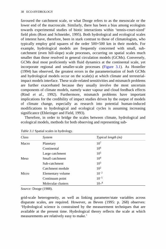
favoured the catchment scale, or what Dooge refers to as the mesoscale or thelower end of the macroscale. Similarly, there has been a bias among ecologiststowards experimental studies of biotic interactions within ‘tennis-court-sized’field plots (Root and Schneider, 1995). Both hydrological and ecological scalesof interest have, therefore, been in stark contrast to those of climatologists, whotypically employ grid squares of the order 500×500 km in their models. Forexample, hydrological models are frequently concerned with small, sub-catchment (even hill-slope) scale processes, occurring on spatial scales muchsmaller than those resolved in general circulation models (GCMs). Conversely,GCMs deal most proficiently with fluid dynamics at the continental scale, yetincorporate regional and smaller-scale processes (Figure 3.1). As Hosteller(1994) has observed, the greatest errors in the parameterisation of both GCMsand hydrological models occur on the scale(s) at which climate and terrestrial-impact models interface. These scale-related sensitivities and mismatch problemsare further exacerbated because they usually involve the most uncertaincomponents of climate models, namely water vapour and cloud feedback effects(Rind et al., 1992). Furthermore, mismatch problems have importantimplications for the credibility of impact studies driven by the output of modelsof climate change, especially as research into potential human-inducedmodifications to hydrological and ecological cycles is assuming increasingsignificance (Ehleringer and Field, 1993).
Therefore, in order to bridge the scales between climate, hydrological andecological models, methods for both observing and representing sub-
Table 3.1 Spatial scales in hydrology.
Class System Typical length (m)
Macro Planetary 107
Continental 106
Large catchment 105
Meso Small catchment 104
Sub-catchment 103
Catchment module 102
Micro Elementary volume 10−2
Continuum point 10−5
Molecular clusters 10–8
Source: Dooge (1988).
grid-scale heterogeneity, as well as linking parameter/state variables acrossdisparate scales, are required. However, as Beven (1995: p. 268) observes:‘Hydrological science is constrained by the measurement techniques that areavailable at the present time. Hydrological theory reflects the scale at whichmeasurements are relatively easy to make.’
38 ECO-HYDROLOGY
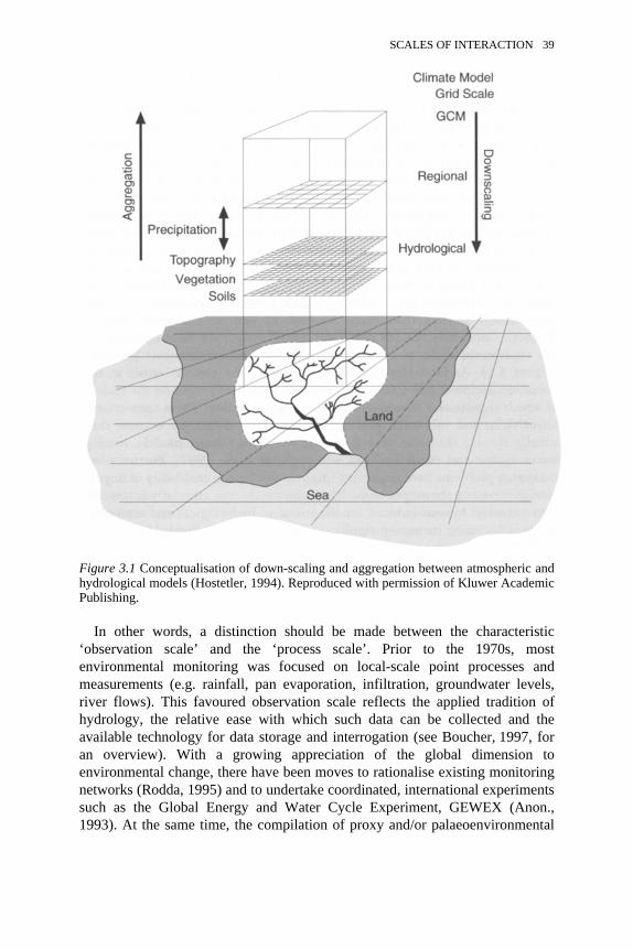
In other words, a distinction should be made between the characteristic‘observation scale’ and the ‘process scale’. Prior to the 1970s, mostenvironmental monitoring was focused on local-scale point processes andmeasurements (e.g. rainfall, pan evaporation, infiltration, groundwater levels,river flows). This favoured observation scale reflects the applied tradition ofhydrology, the relative ease with which such data can be collected and theavailable technology for data storage and interrogation (see Boucher, 1997, foran overview). With a growing appreciation of the global dimension toenvironmental change, there have been moves to rationalise existing monitoringnetworks (Rodda, 1995) and to undertake coordinated, international experimentssuch as the Global Energy and Water Cycle Experiment, GEWEX (Anon.,1993). At the same time, the compilation of proxy and/or palaeoenvironmental
Figure 3.1 Conceptualisation of down-scaling and aggregation between atmospheric andhydrological models (Hostetler, 1994). Reproduced with permission of Kluwer AcademicPublishing.
SCALES OF INTERACTION 39
data sets has enabled the reconstruction of hydrometeorological andpalaeoecological time series, and has involved a greater range of scientificdisciplines in eco-hydrological research (Barker and Higgitt, 1997). Similarly,archival and documentary evidence is increasingly employed to augmentinstrumental records and to construct homogeneous data sets for key hydrologicalvariables such as rainfall (Jones and Conway, 1997) and temperature (Parker et al.,1992).
Despite these contributions, there is still a paucity of near-surface data for theoceans and many remote or mountainous regions of the world. However,remotely sensed (satellite and radar) information has provided hydrologists andecologists with new opportunities to observe non-point processes at resolutions ofa few metres to the global scale. Remote sensing now routinely provides data forhydrological model parameter estimation, computations of soil moisture and flowregimes, and for real-time flood forecasting (Schultz, 1988). Indeed, remotesensing is capable of quantifying all the key hydrological fluxes and storages ofthe water balance equation (i.e. precipitation, evapotranspiration, snow cover,runoff and soil moisture) to resolutions of 10−30 m (Engman and Gurney, 1991).This capability has facilitated what Shuttleworth (1988) terms‘macrohydrology’: the study of global atmosphere-hydrosphere-biosphererelations and feedbacks. For example, Oki et al. (1995) used atmospheric vapourflux convergence in conjunction with atmospheric water balance calculations toestimate monthly discharge for nearly seventy large rivers and to produce globalfreshwater runoff volumes.
By calculating ratios of the upwelling land surface reflectance in the red andinfrared portions of the electromagnetic spectrum, satellite sensors such as theAdvanced Very High Resolution Radiometer (AVHRR) can also be used toderive areal averages of photosynthetically active biomass, albedo, canopyresistance, leaf area index and fractional vegetation cover (Xinmei et al., 1995).For example, the normalised difference vegetation index (NDVI) (Tucker andSellers, 1986) has been used to study vegetation phenology (Justice et al., 1986)and to monitor vegetation changes over whole continents in relation to shifts inprecipitation (Tucker et al., 1991) or El Niño-related droughts (Anyamba andEastman, 1996). NDVI data are also used to monitor crops, and as a majorbiophysical indicator in drought and famine early warning systems such as theGlobal Early Warning System (GEWS) of the Food and AgriculturalOrganisation (FAO) (Henricksen, 1986; Hutchinson, 1991).
Two technological developments have afforded visualisation and quantitativemodelling of eco-hydrological problems, namely geographical informationsystems (GIS) and digital terrain models (DTM). GIS systems allow theorganisation and display of digitised terrain attributes such as soil type,vegetation or raw elevation data to represent the three-dimensional properties ofa landscape. Such powerful data interrogation and visualisation techniques havebeen enabled by the increasing computational speed and data storage capabilitiesof modern PCs and work stations. Together, GIS and DTM have facilitated many
40 ECO-HYDROLOGY
new hydrological, geomorphological and biological applications (see Moore etal., 1991). Although Grayson et al. (1993) asserted that GIS are ‘hydrologicallyneutral’ they have nonetheless allowed hydrologists to theorise and work in waysthat previously would not have been practicable. McDonnell (1996) noted thatvaluable hydrological research has already been undertaken using GIS in therealms of parameter estimation, loosely coupled hydrological models, integratedmodelling and the assembly of hydrological inventories. For example, recentapplications of GIS and DTM include the estimation of hydrologically relevantgeomorphological parameters from topographic information (Gyasi-Agyei et al.,1995); physically based modelling of spatial variations in soil depth as a functionof topographic position (Dietrich et al., 1995); and the regionalisation (orclassification) of catchment behaviour based on ‘hydrological response units’(Flügel, 1995). According to Sivapalan and Kalma (1995), the availability ofboth GIS and DTM has revolutionised hydrology, but their use is still undergoingrapid development (often uncritically), and a number of scale problemsassociated with their use are often ignored. At the same time, GIS and DTM havealso presented new opportunities for investigating the effect of scale andheterogeneity on eco-hydrological processes (see below).
PROCESS SCALES, HETEROGENEITY ANDVARIABILITY
Earlier, a clear distinction was made between characteristic observation andprocess scales: the former is traditionally a point (or more recently a ‘grid-boxaverage’); the latter often exhibits variations across both space and time. As thefollowing discussion will show, because the observation and process scalesseldom correspond, inferences must be made concerning the nature of theheterogeneity, variability and process scaling. By convention, the term‘heterogeneity’ is typically used to describe spatial variations in media properties(such as soil hydraulic conductivity), whereas ‘variability’ refers to fluxes thatvary in space and/or time (such as rainfall).
For example, at the local scale (1 m), the dominant flow pathway may be viasoil macropores; at the hill-slope scale (100 m), preferential flow may occurthrough high-conductivity soil horizons or pipes; at the catchment scale (10 km),the drainage network may reflect underlying differences in soil types; and at theregional scale (1000 km), the stream network density may correspond tovariations in geology and/or climate. Similarly, variability in time is also presentat a range of scales: at the event scale (hours or days), the shape of the floodhydrograph is governed by the characteristics of the precipitation event and bythe receiving catchment; at the seasonal scale (months to years), the flow regimemay be strongly influenced by physioclimatic controls on rainfall, snowmelt andevaporation; and at the long-term scale (decades or centuries), runoff mayexhibit variability due to land-use, climate or anthropic changes. By way of anexample, Figure 3.2 shows spatial and temporal scales of rainfall in relation to a
SCALES OF INTERACTION 41
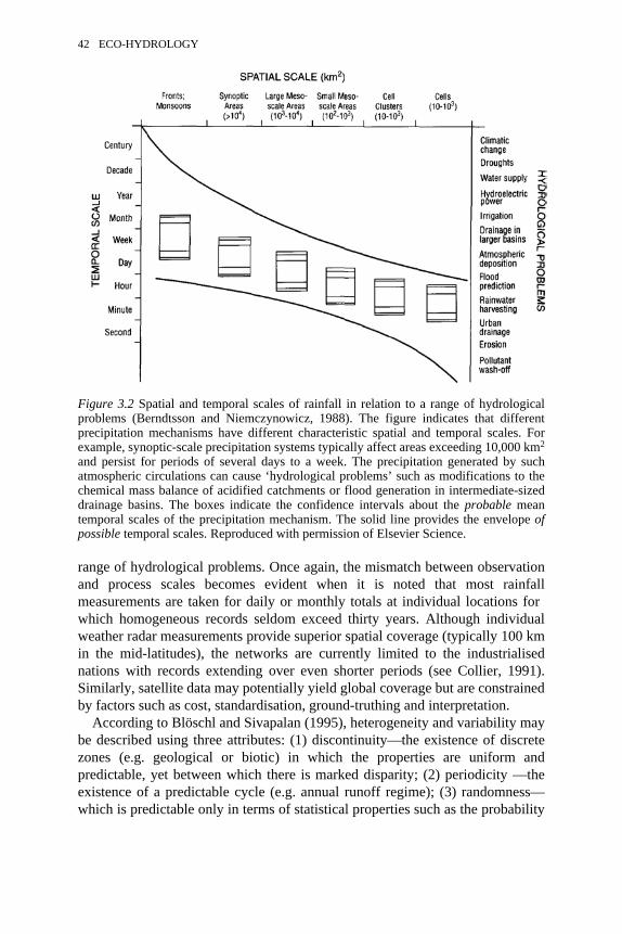
range of hydrological problems. Once again, the mismatch between observationand process scales becomes evident when it is noted that most rainfallmeasurements are taken for daily or monthly totals at individual locations for which homogeneous records seldom exceed thirty years. Although individualweather radar measurements provide superior spatial coverage (typically 100 kmin the mid-latitudes), the networks are currently limited to the industrialisednations with records extending over even shorter periods (see Collier, 1991).Similarly, satellite data may potentially yield global coverage but are constrainedby factors such as cost, standardisation, ground-truthing and interpretation.
According to Blöschl and Sivapalan (1995), heterogeneity and variability maybe described using three attributes: (1) discontinuity—the existence of discretezones (e.g. geological or biotic) in which the properties are uniform andpredictable, yet between which there is marked disparity; (2) periodicity —theexistence of a predictable cycle (e.g. annual runoff regime); (3) randomness—which is predictable only in terms of statistical properties such as the probability
Figure 3.2 Spatial and temporal scales of rainfall in relation to a range of hydrologicalproblems (Berndtsson and Niemczynowicz, 1988). The figure indicates that differentprecipitation mechanisms have different characteristic spatial and temporal scales. Forexample, synoptic-scale precipitation systems typically affect areas exceeding 10,000 km2
and persist for periods of several days to a week. The precipitation generated by suchatmospheric circulations can cause ‘hydrological problems’ such as modifications to thechemical mass balance of acidified catchments or flood generation in intermediate-sizeddrainage basins. The boxes indicate the confidence intervals about the probable meantemporal scales of the precipitation mechanism. The solid line provides the envelope ofpossible temporal scales. Reproduced with permission of Elsevier Science.
42 ECO-HYDROLOGY
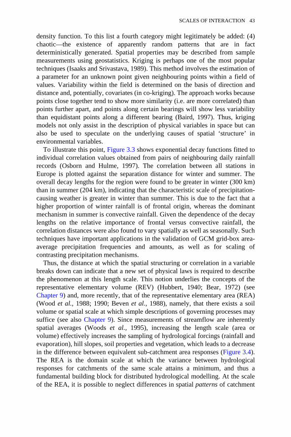
density function. To this list a fourth category might legitimately be added: (4)chaotic—the existence of apparently random patterns that are in factdeterministically generated. Spatial properties may be described from samplemeasurements using geostatistics. Kriging is perhaps one of the most populartechniques (Isaaks and Srivastava, 1989). This method involves the estimation ofa parameter for an unknown point given neighbouring points within a field ofvalues. Variability within the field is determined on the basis of direction anddistance and, potentially, covariates (in co-kriging). The approach works becausepoints close together tend to show more similarity (i.e. are more correlated) thanpoints further apart, and points along certain bearings will show less variabilitythan equidistant points along a different bearing (Baird, 1997). Thus, krigingmodels not only assist in the description of physical variables in space but canalso be used to speculate on the underlying causes of spatial ‘structure’ inenvironmental variables.
To illustrate this point, Figure 3.3 shows exponential decay functions fitted toindividual correlation values obtained from pairs of neighbouring daily rainfallrecords (Osborn and Hulme, 1997). The correlation between all stations inEurope is plotted against the separation distance for winter and summer. Theoverall decay lengths for the region were found to be greater in winter (300 km)than in summer (204 km), indicating that the characteristic scale of precipitation-causing weather is greater in winter than summer. This is due to the fact that ahigher proportion of winter rainfall is of frontal origin, whereas the dominantmechanism in summer is convective rainfall. Given the dependence of the decaylengths on the relative importance of frontal versus convective rainfall, thecorrelation distances were also found to vary spatially as well as seasonally. Suchtechniques have important applications in the validation of GCM grid-box area-average precipitation frequencies and amounts, as well as for scaling ofcontrasting precipitation mechanisms.
Thus, the distance at which the spatial structuring or correlation in a variablebreaks down can indicate that a new set of physical laws is required to describethe phenomenon at this length scale. This notion underlies the concepts of therepresentative elementary volume (REV) (Hubbert, 1940; Bear, 1972) (seeChapter 9) and, more recently, that of the representative elementary area (REA)(Wood et al., 1988; 1990; Beven et al., 1988), namely, that there exists a soilvolume or spatial scale at which simple descriptions of governing processes maysuffice (see also Chapter 9). Since measurements of streamflow are inherentlyspatial averages (Woods et al., 1995), increasing the length scale (area orvolume) effectively increases the sampling of hydrological forcings (rainfall andevaporation), hill slopes, soil properties and vegetation, which leads to a decreasein the difference between equivalent sub-catchment area responses (Figure 3.4).The REA is the domain scale at which the variance between hydrologicalresponses for catchments of the same scale attains a minimum, and thus afundamental building block for distributed hydrological modelling. At the scaleof the REA, it is possible to neglect differences in spatial patterns of catchment
SCALES OF INTERACTION 43
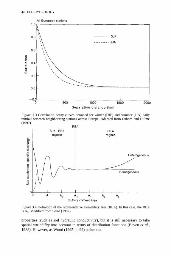
properties (such as soil hydraulic conductivity), but it is still necessary to takespatial variability into account in terms of distribution functions (Beven et al.,1988). However, as Wood (1995: p. 92) points out:
Figure 3.3 Correlation decay curves obtained for winter (DJF) and summer (JJA) dailyrainfall between neighbouring stations across Europe. Adapted from Osborn and Hulme(1997).
Figure 3.4 Definition of the representative elementary area (REA). In this case, the REAis A3. Modified from Baird (1997).
44 ECO-HYDROLOGY
this transition in scale, where pattern no longer becomes important but onlyits statistical representation, may occur at different spatial scales fordifferent processes, may vary temporally for the same parameter (exceptduring wet or dry periods) and may vary with the scale of the ‘macroscale’model. Much of the research to date may indicate that the REA forcatchment modelling is…[in the region of] 0.1 to 25 km2.
Theoretically, an REA may be derived for any spatially averaged environmentalparameter, but its precise value will be process-, region- and time-specific. Forexample, Blöschl et al. (1995) showed that the REA size is strongly governed bythe correlation length of precipitation fields and by the storm duration.
The characterisation of spatial heterogeneities in land surface-atmosphereinteractions at all length scales also remains a great challenge to hydro-meteorologists, because the characteristics of the atmosphere above dry and wet(vegetated) surfaces are significantly different due to the contrasting processes ofenergy redistribution at the ground surface. Avissar (1995) identified five land-surface characteristics that need to be specified accurately in atmosphericmodels, namely, stomatal conductance, soil surface wetness, surface roughness,leaf area index and albedo. Under stable weather conditions, spatial-variability ofany of these characteristics of the order of 100 km was found to inducemesoscale circulations in models of the transport of heat and moisture in theplanetary boundary layer. Such circulations were observable for length scales aslow as 10 km and were sufficient to promote non-linear feedbacks arising fromcloud formation and precipitation. In a similar analysis, Shuttleworth (1988)made a distinction between disorganised and organised variability, also forlength scales of 10 km (Figure 3.5). Under conditions of disorganised variabilityat length scales of 10 km or less, fluid flow and mixing processes naturallyintegrate the land-atmosphere feedbacks, but under conditions of organisedvariability at length scales greater than 10 km, there may be an organised(convective) response in the atmosphere that alters the effective value of surfaceproperties at GCM sub-grid scales.
Both studies suggest that spatial variability in land-surface parameters overlength scales of the order 10 km is sufficient to induce non-linear feedbacks, principally through modified spatial patterns of rainfall and surface energyredistribution. However, many state-of-the-art atmospheric models have adoptedparameterisations of land-surface processes at smaller scales at which spatialhomogeneity is assumed. Even statistical descriptions of heterogeneity fail tocapture lateral interactions between contrasting vegetation surfaces, suggestingthat mesoscale circulations must be considered explicitly (Avissar, 1995).Changed energy fluxes and wind regimes have also been associated with changesfrom tall evergreen vegetation to the alternating short annual vegetation and baresoils associated with agriculture. For example, Hobbs (1994) has describedprofound changes in nutrient, energy and water fluxes as a result of thefragmentation of native perennial vegetation in Western Australia by the
SCALES OF INTERACTION 45
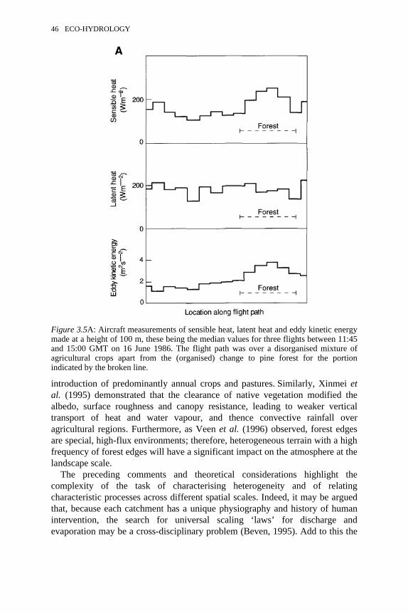
introduction of predominantly annual crops and pastures. Similarly, Xinmei etal. (1995) demonstrated that the clearance of native vegetation modified thealbedo, surface roughness and canopy resistance, leading to weaker verticaltransport of heat and water vapour, and thence convective rainfall overagricultural regions. Furthermore, as Veen et al. (1996) observed, forest edgesare special, high-flux environments; therefore, heterogeneous terrain with a highfrequency of forest edges will have a significant impact on the atmosphere at thelandscape scale.
The preceding comments and theoretical considerations highlight thecomplexity of the task of characterising heterogeneity and of relatingcharacteristic processes across different spatial scales. Indeed, it may be arguedthat, because each catchment has a unique physiography and history of humanintervention, the search for universal scaling ‘laws’ for discharge andevaporation may be a cross-disciplinary problem (Beven, 1995). Add to this the
Figure 3.5A: Aircraft measurements of sensible heat, latent heat and eddy kinetic energymade at a height of 100 m, these being the median values for three flights between 11:45and 15:00 GMT on 16 June 1986. The flight path was over a disorganised mixture ofagricultural crops apart from the (organised) change to pine forest for the portionindicated by the broken line.
46 ECO-HYDROLOGY
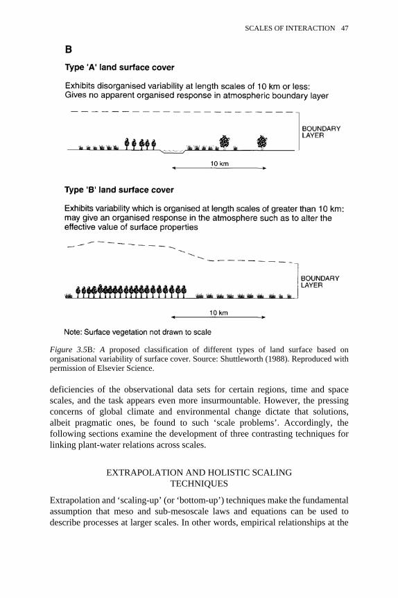
deficiencies of the observational data sets for certain regions, time and spacescales, and the task appears even more insurmountable. However, the pressingconcerns of global climate and environmental change dictate that solutions,albeit pragmatic ones, be found to such ‘scale problems’. Accordingly, thefollowing sections examine the development of three contrasting techniques forlinking plant-water relations across scales.
EXTRAPOLATION AND HOLISTIC SCALINGTECHNIQUES
Extrapolation and ‘scaling-up’ (or ‘bottom-up’) techniques make the fundamentalassumption that meso and sub-mesoscale laws and equations can be used todescribe processes at larger scales. In other words, empirical relationships at the
Figure 3.5B: A proposed classification of different types of land surface based onorganisational variability of surface cover. Source: Shuttleworth (1988). Reproduced withpermission of Elsevier Science.
SCALES OF INTERACTION 47

plant scale are applicable at the canopy, patch and biome scales. The macroscaleparameters used in the meso and sub-mesoscale equations are often termed‘effective parameters’. These parameters must characterise all points within amodel domain, such that a model based on the uniform parameter field yields thesame response as a model based on a heterogeneous parameter field (Blöschl andSivapalan, 1995). However, as Dawson and Chapin (1993: p. 318) point out,there is always the danger that ‘[too much] information about detailedmechanisms may be inefficient, incorporating excessive detail and ignoring otheraspects that are critical to understanding processes at the higher levels.’
Thus, processes underlying larger-scale responses may be obscured by noisy orunrelated local variations. For example, Figure 3.6 shows spatial variations in‘greenness’ obtained from a composite image (visible red, near infrared and nearmiddle infrared) of the LANDSAT Thematic Mapper in which each pixelrepresents an area of 30 m2. Figure 3.6A shows the entire image covering theDerbyshire Peak District, Nottinghamshire and parts of north Leicestershire, UK.At this scale, the principal factors governing the vegetation distribution aregeological and climatological. A clear distinction between the vegetationoverlying the gritstone and limestone is evident in the northwest corner of theimage. To the northeast, the geology is sandstone, while the south and southwestcomprise Keuper marl overlying Coal Measures. At the mesoscale (catchment),variations in vegetation reflect land management practices and proximity to theriver floodplain (Figure 3.6B). Finally, at the scale of individual fields (Figure 3.6C) spatial variations in the vegetation primarily reflect soil moisture, which inturn is governed by local topography, field drainage and soil properties. Hence, itis improbable that the significance of geological or climatological controls tospatial variations in the vegetation cover evident at the regional scale(Figure 3.6A) could be inferred from the observable information at the field scale(Figure 3.6C).
Nonetheless, the most straightforward up-scaling approach is to assume thatthe parameters at the meso and sub-mesoscale are the same as those at largerscales. The scaling problem then becomes a matter of multiplying by the newlength scale or catchment area. For example, Kuczera (1985) modelled observedreductions in river catchment runoff following bushfires in the eucalyptus forestsof the Melbourne water supply district, Australia, as a function of stand age:
(3.1)where Yt is the average yield reduction (mm) relative to mature mountain ashforests t years after the bushfire, Lmax is the maximum yield reduction (mm) and1/K is the time to maximum yield reduction (years). Regional relationships werethen established between the two parameters Lmax and K using forestdescriptors such as the percentage of the catchment area covered by regrowtheucalyptus forest. The model was subsequently adapted by Wilby and Gell(1994) to simulate the effect of piecemeal forest harvesting on downstreamrunoff yields entering a sensitive wetland site (Figure 3.7). In both cases, the
48 ECO-HYDROLOGY
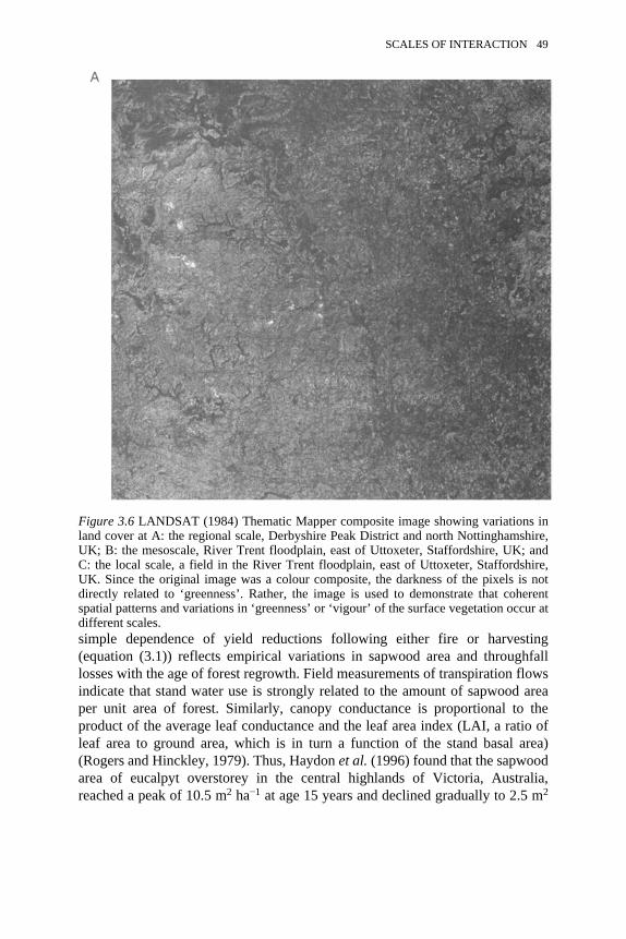
simple dependence of yield reductions following either fire or harvesting(equation (3.1)) reflects empirical variations in sapwood area and throughfalllosses with the age of forest regrowth. Field measurements of transpiration flowsindicate that stand water use is strongly related to the amount of sapwood areaper unit area of forest. Similarly, canopy conductance is proportional to theproduct of the average leaf conductance and the leaf area index (LAI, a ratio ofleaf area to ground area, which is in turn a function of the stand basal area)(Rogers and Hinckley, 1979). Thus, Haydon et al. (1996) found that the sapwoodarea of eucalpyt overstorey in the central highlands of Victoria, Australia,reached a peak of 10.5 m2 ha−1 at age 15 years and declined gradually to 2.5 m2
Figure 3.6 LANDSAT (1984) Thematic Mapper composite image showing variations inland cover at A: the regional scale, Derbyshire Peak District and north Nottinghamshire,UK; B: the mesoscale, River Trent floodplain, east of Uttoxeter, Staffordshire, UK; andC: the local scale, a field in the River Trent floodplain, east of Uttoxeter, Staffordshire,UK. Since the original image was a colour composite, the darkness of the pixels is notdirectly related to ‘greenness’. Rather, the image is used to demonstrate that coherentspatial patterns and variations in ‘greenness’ or ‘vigour’ of the surface vegetation occur atdifferent scales.
SCALES OF INTERACTION 49

50 ECO-HYDROLOGY
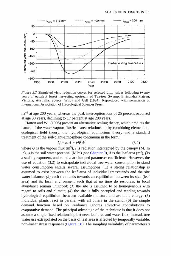
ha−1 at age 200 years, whereas the peak interception loss of 25 percent occurredat age 30 years, declining to 17 percent at age 200 years.
Hatton and Wu (1995) present an alternative scaling theory, which predicts thenature of the water vapour flux/leaf area relationship by combining elements ofecological field theory, the hydrological equilibrium theory and a standardtreatment of the soil-plant-atmosphere continuum in the form:
(3.2)where Q is the vapour flux (m3), I is radiation intercepted by the canopy (MJ m−2), ψ is the soil water potential (MPa) (see Chapter 9), A is the leaf area (m2), f isa scaling exponent, and a and b are lumped parameter coefficients. However, theuse of equation (3.2) to extrapolate individual tree water consumption to standwater consumption entails several assumptions: (1) a strong relationship isassumed to exist between the leaf area of individual trees/stands and the sitewater balance; (2) each tree tends towards an equilibrium between its size (leafarea) and its local environment such that at no time do resources in localabundance remain untapped; (3) the site is assumed to be homogeneous withregard to soils and climate; (4) the site is fully occupied and tending towardshydrological equilibrium between available moisture and available energy; (5)individual plants react in parallel with all others in the stand; (6) the simpledemand function based on irradiance ignores advective contributions toevaporative demand. The principal advantage of the technique is that it does notassume a single fixed relationship between leaf area and water flux; instead, treewater use extrapolated on the basis of leaf area is affected by temporally variable,non-linear stress responses (Figure 3.8). The sampling variability of parameters a
Figure 3.7 Simulated yield reduction curves for selected Lmax values following twentyyears of eucalypt forest harvesting upstream of Tea-tree Swamp, Errinundra Plateau,Victoria, Australia. Source: Wilby and Gell (1994). Reproduced with permission ofInternational Association of Hydrological Sciences Press.
SCALES OF INTERACTION 51
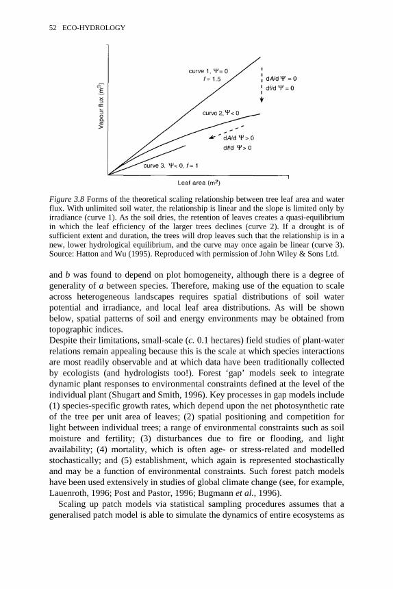
and b was found to depend on plot homogeneity, although there is a degree ofgenerality of a between species. Therefore, making use of the equation to scaleacross heterogeneous landscapes requires spatial distributions of soil waterpotential and irradiance, and local leaf area distributions. As will be shownbelow, spatial patterns of soil and energy environments may be obtained fromtopographic indices. Despite their limitations, small-scale (c. 0.1 hectares) field studies of plant-waterrelations remain appealing because this is the scale at which species interactionsare most readily observable and at which data have been traditionally collectedby ecologists (and hydrologists too!). Forest ‘gap’ models seek to integratedynamic plant responses to environmental constraints defined at the level of theindividual plant (Shugart and Smith, 1996). Key processes in gap models include(1) species-specific growth rates, which depend upon the net photosynthetic rateof the tree per unit area of leaves; (2) spatial positioning and competition forlight between individual trees; a range of environmental constraints such as soilmoisture and fertility; (3) disturbances due to fire or flooding, and lightavailability; (4) mortality, which is often age- or stress-related and modelledstochastically; and (5) establishment, which again is represented stochasticallyand may be a function of environmental constraints. Such forest patch modelshave been used extensively in studies of global climate change (see, for example,Lauenroth, 1996; Post and Pastor, 1996; Bugmann et al., 1996).
Scaling up patch models via statistical sampling procedures assumes that ageneralised patch model is able to simulate the dynamics of entire ecosystems as
Figure 3.8 Forms of the theoretical scaling relationship between tree leaf area and waterflux. With unlimited soil water, the relationship is linear and the slope is limited only byirradiance (curve 1). As the soil dries, the retention of leaves creates a quasi-equilibriumin which the leaf efficiency of the larger trees declines (curve 2). If a drought is ofsufficient extent and duration, the trees will drop leaves such that the relationship is in anew, lower hydrological equilibrium, and the curve may once again be linear (curve 3).Source: Hatton and Wu (1995). Reproduced with permission of John Wiley & Sons Ltd.
52 ECO-HYDROLOGY
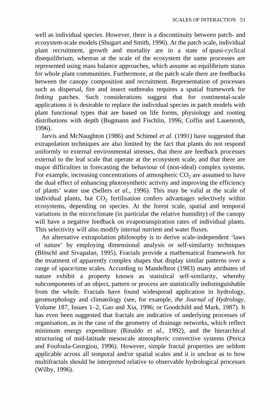
well as individual species. However, there is a discontinuity between patch- andecosystem-scale models (Shugart and Smith, 1996). At the patch scale, individualplant recruitment, growth and mortality are in a state of quasi-cyclicaldisequilibrium, whereas at the scale of the ecosystem the same processes arerepresented using mass balance approaches, which assume an equilibrium statusfor whole plant communities. Furthermore, at the patch scale there are feedbacksbetween the canopy composition and recruitment. Representation of processessuch as dispersal, fire and insect outbreaks requires a spatial framework forlinking patches. Such considerations suggest that for continental-scaleapplications it is desirable to replace the individual species in patch models withplant functional types that are based on life forms, physiology and rootingdistributions with depth (Bugmann and Fischlin, 1996; Coffin and Lauenroth,1996).
Jarvis and McNaughton (1986) and Schimel et al. (1991) have suggested thatextrapolation techniques are also limited by the fact that plants do not responduniformly to external environmental stresses, that there are feedback processesexternal to the leaf scale that operate at the ecosystem scale, and that there aremajor difficulties in forecasting the behaviour of (non-ideal) complex systems.For example, increasing concentrations of atmospheric CO2 are assumed to havethe dual effect of enhancing photosynthetic activity and improving the efficiencyof plants’ water use (Sellers et al., 1996). This may be valid at the scale ofindividual plants, but CO2 fertilisation confers advantages selectively withinecosystems, depending on species. At the forest scale, spatial and temporalvariations in the microclimate (in particular the relative humidity) of the canopywill have a negative feedback on evapotranspiration rates of individual plants.This selectivity will also modify internal nutrient and water fluxes.
An alternative extrapolation philosophy is to derive scale-independent ‘lawsof nature’ by employing dimensional analysis or self-similarity techniques(Blöschl and Sivapalan, 1995). Fractals provide a mathematical framework forthe treatment of apparently complex shapes that display similar patterns over arange of space/time scales. According to Mandelbrot (1983) many attributes ofnature exhibit a property known as statistical self-similarity, wherebysubcomponents of an object, pattern or process are statistically indistinguishablefrom the whole. Fractals have found widespread application in hydrology,geomorphology and climatology (see, for example, the Journal of Hydrology,Volume 187, Issues 1–2, Gao and Xia, 1996; or Goodchild and Mark, 1987). Ithas even been suggested that fractals are indicative of underlying processes oforganisation, as in the case of the geometry of drainage networks, which reflectminimum energy expenditure (Rinaldo et al., 1992), and the hierarchicalstructuring of mid-latitude mesoscale atmospheric convective systems (Pericaand Foufoula-Georgiou, 1996). However, simple fractal properties are seldomapplicable across all temporal and/or spatial scales and it is unclear as to howmultifractals should be interpreted relative to observable hydrological processes(Wilby, 1996).
SCALES OF INTERACTION 53
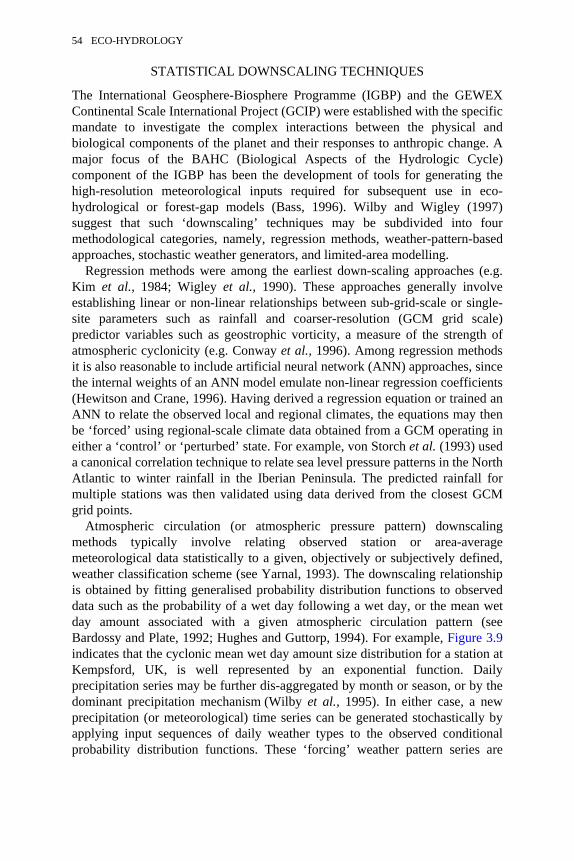
STATISTICAL DOWNSCALING TECHNIQUES
The International Geosphere-Biosphere Programme (IGBP) and the GEWEXContinental Scale International Project (GCIP) were established with the specificmandate to investigate the complex interactions between the physical andbiological components of the planet and their responses to anthropic change. Amajor focus of the BAHC (Biological Aspects of the Hydrologic Cycle)component of the IGBP has been the development of tools for generating thehigh-resolution meteorological inputs required for subsequent use in eco-hydrological or forest-gap models (Bass, 1996). Wilby and Wigley (1997)suggest that such ‘downscaling’ techniques may be subdivided into fourmethodological categories, namely, regression methods, weather-pattern-basedapproaches, stochastic weather generators, and limited-area modelling.
Regression methods were among the earliest down-scaling approaches (e.g.Kim et al., 1984; Wigley et al., 1990). These approaches generally involveestablishing linear or non-linear relationships between sub-grid-scale or single-site parameters such as rainfall and coarser-resolution (GCM grid scale)predictor variables such as geostrophic vorticity, a measure of the strength ofatmospheric cyclonicity (e.g. Conway et al., 1996). Among regression methodsit is also reasonable to include artificial neural network (ANN) approaches, sincethe internal weights of an ANN model emulate non-linear regression coefficients(Hewitson and Crane, 1996). Having derived a regression equation or trained anANN to relate the observed local and regional climates, the equations may thenbe ‘forced’ using regional-scale climate data obtained from a GCM operating ineither a ‘control’ or ‘perturbed’ state. For example, von Storch et al. (1993) useda canonical correlation technique to relate sea level pressure patterns in the NorthAtlantic to winter rainfall in the Iberian Peninsula. The predicted rainfall formultiple stations was then validated using data derived from the closest GCMgrid points.
Atmospheric circulation (or atmospheric pressure pattern) downscalingmethods typically involve relating observed station or area-averagemeteorological data statistically to a given, objectively or subjectively defined,weather classification scheme (see Yarnal, 1993). The downscaling relationshipis obtained by fitting generalised probability distribution functions to observeddata such as the probability of a wet day following a wet day, or the mean wetday amount associated with a given atmospheric circulation pattern (seeBardossy and Plate, 1992; Hughes and Guttorp, 1994). For example, Figure 3.9indicates that the cyclonic mean wet day amount size distribution for a station atKempsford, UK, is well represented by an exponential function. Dailyprecipitation series may be further dis-aggregated by month or season, or by thedominant precipitation mechanism (Wilby et al., 1995). In either case, a newprecipitation (or meteorological) time series can be generated stochastically byapplying input sequences of daily weather types to the observed conditionalprobability distribution functions. These ‘forcing’ weather pattern series are
54 ECO-HYDROLOGY
typically generated using either Monte Carlo techniques (Wilby, 1994) or thepressure fields of GCMs (Matyasovszky el al., 1994). Although the majority ofsuch studies have focused on daily precipitation, series of daily circulationpatterns may be used to downscale other variables such as temperature,evaporation and ultraviolet radiation, or multivariate processes such as floods,droughts, acid deposition, smog, ozone and atmospheric particulates (Bass,1996).
Stochastic weather generators share many attributes of conventionalcirculation-based downscaling models but differ in their means of application tofuture climate conditions. Richardson’s (1981) weather generator (WGEN)model is the most commonly used for climate impact studies: this was originallydesigned to simulate daily time series of precipitation amount, maximum andminimum temperature, and solar radiation for the present climate. Rather than
Figure 3.9 Frequency diagrams of wet day rainfall amounts (mm) at Kempsford in theCotswolds, UK, 1970–1990 corresponding to the cyclonic (C-type) Lamb weather type ondays A: without fronts, and B: with at least one front. Note the increased frequency ofprecipitation events under frontal weather conditions, particularly for days with rainfallexceeding 10 mm.
SCALES OF INTERACTION 55
being conditioned by circulation patterns, all variables in the Richardson modelare simulated conditionally according to previous precipitation occurrence. Atthe heart of all such models are first- or multiple-order Markov renewalprocesses in which, for each successive day, the precipitation occurrence (andpossibly amount) is governed by outcomes on previous days. Models such asWGEN have been adapted for a number of climate change impact studies (e.g.Wilks, 1992; Mearns et al., 1996). There is also the possibility of spatiallydistributing WGEN parameters across landscapes, even in complex terrain, bycombining interpolation techniques and DTMs (see VEMAP study below).However, the principal issue involving the application of WGEN or otherstochastic weather generators to future climates has been the method of adjustingthe parameters in a physically realistic and internally consistent way. Forexample, Katz (1996) demonstrated, using daily observations at Denver,Colorado, that when the WGEN parameters are varied, certain unanticipatedeffects can be produced. Modifying the probability of daily precipitationoccurrence changed not only the mean daily temperature but also its variance andautocorrelation in possibly unrealistic ways.
Given the limitations of GCM grid-point predictions for regional climatechange impact studies, the final downscaling option is to embed a higher-resolution limited-area climate model within the GCM, using the GCM to definethe (time-varying) boundary conditions (Giorgi, 1990; Mearns et al., 1995).Although limited area models (LAMs) can produce climates for 20–50 kmhorizontal grid spacing and 100–1000 m vertical resolution there are severalacknowledged limitations of the approach. LAMs still require considerablecomputing resources and are as expensive to run as a global GCM. Furthermore,they are somewhat inflexible in the sense that the computational demands applyeach time that the model is transferred to a different region. Above all, the LAMis completely dependent upon the veracity of the GCM grid-point data that areused to drive the boundary conditions of the region—a problem that also appliesto circulation-driven downscaling methods.
As Table 3.2 indicates, the confident application of statistical downscalingtechniques to the study of plant-water relations is constrained by several as yetunresolved issues. Perhaps the most serious limitation is the way in whichdownscaling compels the use of ‘passive’ atmosphere-vegetation models; currentmethodologies do not incorporate feedbacks between the land surface andclimate, or permit scale interactions. Furthermore, the majority of downscalingtools relate point or areal averages to regional scale phenomena according to thelevel of data available. However, what is often required for
Table 3.2 Outstanding challenges to the confident application of statistical downscalingtechniques.
• The whole ideology of downscaling presupposes that, as a result of human-induced global warming, there will be significant (and predictable) changes in the
56 ECO-HYDROLOGY
downscaling predictor variables (such as the frequencies of daily weatherpatterns).
• To date, most downscaling studies have been conducted for daily or monthlyprecipitation in temperate, mid-latitude regions of the Northern Hemisphere;relatively few have tackled semi-arid or tropical locations. There has also been atopographic bias towards low-altitude sites.
• There is a need for more general weather classification systems used indownscaling. Most weather classification schemes are inherently parochialbecause of the important controlling influences of regional- and local-scalefactors such as topography or ocean/land distributions.
• The majority of downscaling approaches generate time series of data for only afew hydrologically relevant parameters, most commonly precipitation. There is aneed for techniques that downscale internally consistent multivariate data whichpreserve covariance among parameters and auto-correlation within time series.
• Current downscaling approaches seldom capture climate variability at alltemporal or spatial scales. For example, even within a single circulation pattern,the precipitation statistics may vary considerably from year to year.
• This type of non-stationarity can be accounted for by developing more complexstatistical models (within the constraints of model reliability imposed by dataavailability). This, however, puts greater pressure on the driving GCMs toprovide reliable predictions for a greater range of variables.
• Downscaling is a uni-directional modelling technique. Local- and regional-scalehydrological or ecological responses are forced by mesoscale predictor variables.Current techniques have no means of incorporating terrestrial feedbacks into thedriving climate models.
Source: Adapted from Wilby and Wigley (1997).
impact assessment is a means of interpolating between data-rich regions to data-poor sites. The remaining two sections will address these important scale issues.
DISTRIBUTING TECHNIQUES
Some commentators have suggested that a general theory of hydrological scalingis unlikely to exist and that sub-grid-scale heterogeneity should be treatedstatistically (Beven, 1995: p. 278):
the hydrological system is greatly influenced by external historical andgeological forcings. This greatly limits the potential for scale-invariantbehaviour and it is suggested that it may be better to recognise explicitly thatscale-dependent models are required in which the characterisation of theheterogeneity of responses is posed as a problem of sub-grid scaleparameterisation.
As was noted earlier, hydrological and ecological measurements tend to have acoarser spatial than temporal resolution, prompting the widespread use ofinterpolation techniques for the space domain. Perhaps the most thoroughly
SCALES OF INTERACTION 57
discussed interpolation problem in hydrology is the spatial estimation of rainfallfrom point rain-gauge measurements (see, for example, Shaw, 1994; Reed andStewart, 1994). The problem arises because the measurements on which theinterpolation techniques are based are too widely spaced relative to the naturalvariability of rainfall. For example, the average spacing of hourly rain-gauges inthe relatively dense monitoring network of the British Isles is between 15 and30km (Faulkner and Reynard, personal communication), whereas the lengthscales of individual storm cells are of the order of 10 km (see Figure 3.2).Although the UK Meteorological Office’s MORECS predictions of potential andactual evapotranspiration have a grid spacing of 40 km, rainfall radar typicallyhas a resolution of 2 km, and remotely sensed AVHRR satellite imagery pixelsof 1 km, the widespread use of these data sources is constrained by their highcost and short record lengths relative to surface networks (e.g. AVHRR providesabout fifteen years of data).
Given the constraints of both remote and surface monitoring systems, and thenatural heterogeneity of surface processes, one solution is to correlate thevariable of interest to an auxiliary variable whose spatial distribution is morereadily obtained. The spatial distribution of the dependent variable is theninferred from the spatial distribution of the covariate (Blöschl and Sivapalan,1995). To date, one of the most widely used covariates in eco-hydrology hasbeen topography, for which data with a resolution of 50 m are often available indigital form. The availability of digital elevations and other environmentalvariables such as soils and geology, coupled with GIS and DTM software formanipulating data, has favoured the development of predictive mappingtechniques in the last twenty years. As Table 3.3 indicates, topography can beused to infer the spatial distribution of a wide variety of secondary variables. Forexample, the precipitation-elevation regressions on independent slopes model(PRISM) (Daly et al., 1994) simulates precipitation at 10 km grid scales by, first,dividing the terrain into topographical facets of similar aspect; second, regressingpoint precipitation data against elevation for each facet by region; and third,employing these regression equations spatially to extrapolate station precipitationto cells that have similar facets.
Beven’s (1987) solution to the problem of sub-grid-scale hydrologicalparameterisation was the use of spatial distribution functions to represent
Table 3.3 Examples of topographically derived hydrometeorological variables.
• Elevation: daily and seasonal precipitation totals; snow characteristics includingsnow water equivalent; wind speeds; air temperature; soil depth; air and soil waterchemistry.
• Slope: incident solar radiation; soil properties and preferential flow pathways; lateralsubsurface flow rate; soil moisture; transpiration rates; soil water chemistry.
• Aspect: incident solar radiation; precipitation totals; snow accumulation and melting;wind speeds; air temperature; soil moisture; transpiration rates; atmospheric wet anddry deposition.
58 ECO-HYDROLOGY
• Upslope catchment area: precipitation and runoff volume; soil moisture; soilsurface properties; stream network order and main channel length.
• Slope curvature: snow accumulation; subsurface water flow; soil moisture; soillitter accumulation; soil erosion/deposition rates; rill initiation; soil depth andtexture; water-holding capacity; nutrient availability.
local-scale processes governing runoff production. For example, TOPMODEL(Beven and Kirkby, 1979) simulates the scale-dependent dynamics of the stormhydrograph using the distribution function of an index of hydrological similarity,ln(αT0tanβ), where α is the area draining through a point, tanβ is the local slopeangle at that point and T0 is the local downslope transmissivity at soil saturation.These properties, as well as the spatial distribution functions for incomingrainfall intensities, vegetation processes such as throughfall, soil properties anddownslope water velocities, may all be inferred from DTM of the catchmenttopography. Quinn et al. (1995) and Beven (1995) have extended TOPMODELto represent interactions between downslope subsurface flows and wateravailability for transpiration. Figure 3.10 shows the key elements of their simplepatch model, which represents areas of the landscape with broadly similarresponses in terms of evapotranspiration. The model differs from conventionalone-dimensional surface vegetation-atmosphere models in one respect:subsurface water fluxes are able to enter and leave the patch via upslope anddownslope drainage, respectively. The variability in runoff production, soilmoisture and evapotranspiration is then calculated from a linear combination ofpatches of varying topographical, meteorological, soil, geological and vegetationcharacteristics. Although this allows for more realistic modelling of the patch inthe context of the landscape, the spatial distribution of many of the vegetationand soil properties listed in Figure 3.10 must still be specified from the results ofmicrometeorological experiments and available field data. Furthermore, it mustbe recognised that there may be many permutations of patches that give similarhydrological responses in terms of observed evapotranspiration or runoff. Thisequifinality in model behaviour (see Chapter 9) is further exacerbated by thenumber and weighting of patches selected.
These parameterisation issues might be resolved by calibrating semi-distributed hydrological models such as TOPMODEL using the products ofpredictive vegetation mapping. Indeed, predictive vegetation mapping alreadyembraces many of the principles inherent in topographic hydrological models(e.g. Palmer and Van Staden, 1992). Founded in ecological niche theory andgradient analysis, the approach predicts vegetation composition across alandscape given interpolated environmental variables that are related tophysiological tolerances and are derived from digital soil or elevationdata (Table 3.3). For example, Saunders and Bailey (1994) assessed thesignificance of topography-induced heterogeneity in solar radiation budgets(versus the diffusing effects of orographic cloud) to spatial variability in thevegetation coverage of alpine tundra. Similarly, Haines-Young and Chopping
SCALES OF INTERACTION 59

(1996) reviewed the use of landscape indices as a means of predictive mappingfor biodiversity and conservation planning.
However, as Figure 3.11 implies, a clear distinction must be made betweenpotential (or ‘climax’) natural vegetation and actual (observed) vegetationdistributions. The latter reflects variables related to the disturbance history (suchas fire, grazing or other anthropic influences) as well as the underlyingenvironmental gradients (such as soil moisture, light and nutrients). Furthermore,as Franklin (1995) notes, predictive vegetation mapping assumes static,equilibrium, whole-mosaic models of the spatial distribution of biota. Suchmodels can be useful for understanding or predicting biogeographic distributionsof species’ realised niches at the landscape scale but cannot simulate transient
Figure 3.10 Schematic representation of a simple patch model including definitions of allmodel parameters. Source: Beven (1995). Reproduced with permission of John Wiley &Sons Ltd. (Please note: the model equations are not explained here and interested readersshould consult the original paper.)
60 ECO-HYDROLOGY
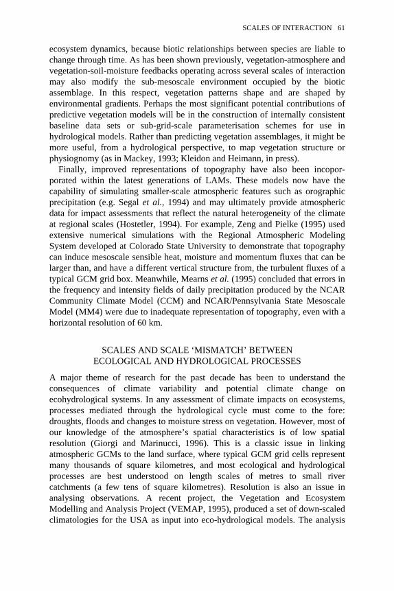
ecosystem dynamics, because biotic relationships between species are liable tochange through time. As has been shown previously, vegetation-atmosphere andvegetation-soil-moisture feedbacks operating across several scales of interactionmay also modify the sub-mesoscale environment occupied by the bioticassemblage. In this respect, vegetation patterns shape and are shaped byenvironmental gradients. Perhaps the most significant potential contributions ofpredictive vegetation models will be in the construction of internally consistentbaseline data sets or sub-grid-scale parameterisation schemes for use inhydrological models. Rather than predicting vegetation assemblages, it might bemore useful, from a hydrological perspective, to map vegetation structure orphysiognomy (as in Mackey, 1993; Kleidon and Heimann, in press).
Finally, improved representations of topography have also been incopor-porated within the latest generations of LAMs. These models now have thecapability of simulating smaller-scale atmospheric features such as orographicprecipitation (e.g. Segal et al., 1994) and may ultimately provide atmosphericdata for impact assessments that reflect the natural heterogeneity of the climateat regional scales (Hostetler, 1994). For example, Zeng and Pielke (1995) usedextensive numerical simulations with the Regional Atmospheric ModelingSystem developed at Colorado State University to demonstrate that topographycan induce mesoscale sensible heat, moisture and momentum fluxes that can belarger than, and have a different vertical structure from, the turbulent fluxes of atypical GCM grid box. Meanwhile, Mearns et al. (1995) concluded that errors inthe frequency and intensity fields of daily precipitation produced by the NCARCommunity Climate Model (CCM) and NCAR/Pennsylvania State MesoscaleModel (MM4) were due to inadequate representation of topography, even with ahorizontal resolution of 60 km.
SCALES AND SCALE ‘MISMATCH’ BETWEENECOLOGICAL AND HYDROLOGICAL PROCESSES
A major theme of research for the past decade has been to understand theconsequences of climate variability and potential climate change onecohydrological systems. In any assessment of climate impacts on ecosystems,processes mediated through the hydrological cycle must come to the fore:droughts, floods and changes to moisture stress on vegetation. However, most ofour knowledge of the atmosphere’s spatial characteristics is of low spatialresolution (Giorgi and Marinucci, 1996). This is a classic issue in linkingatmospheric GCMs to the land surface, where typical GCM grid cells representmany thousands of square kilometres, and most ecological and hydrologicalprocesses are best understood on length scales of metres to small rivercatchments (a few tens of square kilometres). Resolution is also an issue inanalysing observations. A recent project, the Vegetation and EcosystemModelling and Analysis Project (VEMAP, 1995), produced a set of down-scaledclimatologies for the USA as input into eco-hydrological models. The analysis
SCALES OF INTERACTION 61
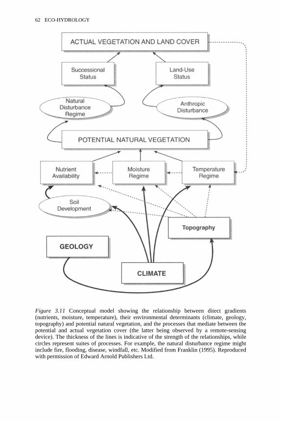
Figure 3.11 Conceptual model showing the relationship between ditect gradients(nutrients, moisture, temperature), their environmental determinants (climate, geology,topography) and potential natural vegetation, and the processes that mediate between thepotential and actual vegetation cover (the latter being observed by a remote-sensingdevice). The thickness of the lines is indicative of the strength of the relationships, whilecircles represent suites of processes. For example, the natural disturbance regime mightinclude fire, flooding, disease, windfall, etc. Modified from Franklin (1995). Reproducedwith permission of Edward Arnold Publishers Ltd.
62 ECO-HYDROLOGY
observations are relatively dense, meteorological station densities average nomore than two per grid cell. While there exist a few areas in the USA and Europewhere patterns of mean climate and interannual variability may be observeddirectly with a resolution of a few kilometres, in most regions precipitation andsurface temperatures may only be estimated from observations with lengthresolutions of 50–100 km. Thus, large-scale studies (e.g. biome or drainage basinscale) must rely on downscaling to account for catchment-scale influences oftopography on temperature, precipitation, radiation and other terrain-dependentaspects of climate (see above). Downscaling procedures intrinsically produce areasonable portrayal of mean conditions, which are strongly constrained byeffects of elevation and orography on precipitation processes and temperature.They do a much worse job with precipitation rates, which depend upon thedynamics of atmospheric processes that intrinsically occur on scales smaller thanthe resolution of typical observing systems: processes on the scale of convectiveand precipitating cloud systems. Thus, capturing even the statistics of stormintensity at a regional scale can be challenging.
There are thus two ‘scale mismatches’ between climate and hydrology: first,between large-scale atmospheric features and small-scale land-surface attributes,in effect, between the resolution of climate models and observations, and thescale of topographic features. This means that terrain-dependent features ofclimate—adiabatic effects, inversions and precipitation —must be inferredindirectly from models and observations. Second, there is a mismatch betweensmall-scale atmospheric features (convective and precipitating clouds) andregional land systems, which makes capturing the occurrence and statistics ofextreme events over large areas difficult.
In considering eco-hydrological systems, there are also key scale ‘matches’.The river catchment or landscape has long been a scale at which both ecologistsand hydrologists could work. Hill slopes provide ordered sequences of soilvariability, moisture availability and vegetation that have been exploited byhydrologists, ecologists and soil scientists (Schimel et al., 1985; Burke et al.,1989). River catchments are a key unit in understanding hydrological processessuch as evapotranspiration, runoff generation and baseflow: they are also anintegrated unit for ecosystem studies, contributing to the understanding ofnutrient budgets and transformations, water use, primary production anddisturbance effects (Borman and Likens, 1979). Catchment studies provide botha scale at which variability within landscapes in ecological and hydrologicalprocesses may be studied (Moldan and Cerny, 1994), and through hydrologicaland hydrochemical gauging, an integrated scale where the aggregate interactionsof climate, hydrology and ecology may be observed and modelled. For example,regional to global nitrogen studies have just begun, and it is evident that gainsand losses of N are highly coupled to water budgets (via leaching) and to soilmoisture variations, the key control over trace gas losses (Mosier et al., 1997;Parton et al., 1996; Figure 3.12). Given the crucial importance of carbon andnitrogen budgets in contemporary ecology and limnology (Schimel et al., in
SCALES OF INTERACTION 63
was conducted on an 0.5° latitude×longitude grid, quite coarse for ecosystemstudies, yet resulting in over 3000 grid cells. Even in the USA, where
press; Hornberger et al., 1994), the catchment scale must be a central focus ofresearch as the scale where phenomena such as leaching and soil moisturestorage may be linked to the biogeochemistry of C and N.
While much of the material reported in this chapter has dealt with interpretingatmospheric information in terms of scales of hydrological and ecologicalprocesses, land-surface processes also affect climate. There is now an extensiveliterature documenting the effects of large-scale modification by the land surfaceof climate (e.g. Melillo et al., 1996). Studies have indicated that deforestationmay affect climate via changes to evapotranspiration and the Bowen ratio, viaalbedo and roughness changes, and via changes to land-surface patch structure,causing mesoscale effects (Dickinson, 1992; Pielke et al., 1991; Henderson-Sellers and McGuffie, 1995). Other studies have looked at global-scale effects ofthe changing land surface on climate via sensitivity studies examining anartificial perturbation to surface conductance (Thompson and Pollard, 1995),simulated effects of doubled atmospheric CO2 concentrations (Sellers et al.,1996), and by a comparison of global ‘potential natural’ to actual vegetation(Chase et al., 1996). Clearly, feedbacks from land-surface hydrology, especiallyvia evapotranspiration, can have substantial effects on climate. Studies of globalhydroclimatological feedbacks using models require that the surface processes becorrectly forced, meaning that changes to the fluxes at the land-atmosphereinterface be correct with regard to the natural scale of the land surface. They alsorequire that land-surface fluxes be correctly aggregated back to the scale of theatmospheric processes simulated, taking into account any processes that arise atsub-grid scales (Zeng and Pielke, 1995). Simulating the coupled effects of landsurface and climate change will be a ‘grand challenge’ for interdisciplinary earthscience in the twenty-first century.
REFERENCES
Anon. (1993) The Global Energy and Water Cycle Experiment (GEWEX), WMO Bulletin42:20–27.
Anyamba, A. and Eastman, J.R. (1996) Interannual variability of NDVI over Africa andits relation to El Niño/Southern Oscillation, International Journal of Remote Sensing17:2533–2548.
Avissar, R. (1995) Scaling of land-atmosphere interactions: an atmospheric modellingperspective, in Kalma, J.D. and Sivapalan, M. (eds) Scale Issues in HydrologicalModelling, Chichester: Wiley, pp. 435–452.
Baird, A.J. (1997) Continuity in hydrological systems, in Wilby, R.L. (ed.) ContemporaryHydrology, Chichester: Wiley, pp. 25–58.
Bardossy, A. and Plate, E.J. (1992) Space-time model for daily rainfall using atmosphericcirculation patterns, Water Resources Research 28:1247–1259.
Barker, P.A. and Higgitt. D. (1997) Palaeohydrology and environmental change indrylands, in Wilby, R.L. (ed.) Contemporary Hydrology. Chichester: Wileypp. 273–316.
64 ECO-HYDROLOGY
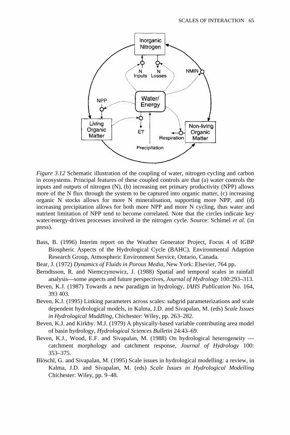
Bass, B. (1996) Interim report on the Weather Generator Project, Focus 4 of IGBPBiospheric Aspects of the Hydrological Cycle (BAHC). Environmental AdaptionResearch Group, Atmospheric Environment Service, Ontario, Canada.
Bear, J. (1972) Dynamics of Fluids in Porous Media, New York: Elsevier, 764 pp.Berndtsson, R. and Niemczynowicz, J. (1988) Spatial and temporal scales in rainfall
analysis—some aspects and future perspectives, Journal of Hydrology 100:293–313.Beven, K.J. (1987) Towards a new paradigm in hydrology, IAHS Publication No. 164,
393 403.Beven, K.J. (1995) Linking parameters across scales: subgrid parameterizations and scale
dependent hydrological models, in Kalma, J.D. and Sivapalan, M. (eds) Scale Issuesin Hydrological Muddling, Chichester: Wiley, pp. 263–282.
Beven, K.J. and Kirkby. M.J. (1979) A physically-based variable contributing area modelof basin hydrology, Hydrological Sciences Bulletin 24:43–69.
Beven, K.J., Wood, E.F. and Sivapalan, M. (1988) On hydrological heterogeneity —catchment morphology and catchment response, Journal of Hydrology 100:353–375.
Blöschl, G. and Sivapalan, M. (1995) Scale issues in hydrological modelling: a review, inKalma, J.D. and Sivapalan, M. (eds) Scale Issues in Hydrological ModellingChichester: Wiley, pp. 9–48.
Figure 3.12 Schematic illustration of the coupling of water, nitrogen cycling and carbonin ecosystems. Principal features of these coupled controls are that (a) water controls theinputs and outputs of nitrogen (N), (b) increasing net primary productivity (NPP) allowsmore of the N flux through the system to be captured into organic matter, (c) increasingorganic N stocks allows for more N mineralisation, supporting more NPP, and (d)increasing precipitation allows for both more NPP and more N cycling, thus water andnutrient limitation of NPP tend to become correlated. Note that the circles indicate keywater/energy-driven processes involved in the nitrogen cycle. Source: Schimel et al. (inpress).
SCALES OF INTERACTION 65
Blöschl, G., Grayson, R.B. and Sivapalan, M. (1995) On the representative elementaryarea (REA) concept and its utility for distributed rainfall-runoff modelling, inKalma, J.D. and Sivapalan, M. (eds) Scale Issues in Hydrological Modelling,Chichester: Wiley. pp. 71–88.
Bormann, F.H., and Likens, G.E. (1979) Pattern and Process in a Forested Ecosystem:Disturbance. Development and the Steady State Based on the Hubbard BrookEcosystem Study, New York: Springer-Verlag, 253 pp.
Boucher, K. (1997) Hydrological monitoring and measurement methods, in Wilby, R.L.(ed.) Contemporary Hydrology, Chichester: Wiley, pp. 107–149.
Bugmann, H.K.M. and Fischlin, A. (1996) Simulating forest dynamics in a complextopography using gridded climatic data, Climatic Change 34:201–211.
Bugmann, H.K.M., Yan, X., Sykes, M.T., Martin, P., Lindner, M., Desanker, P.V. andCumming, S.G. (1996) A comparison of forest gap models: model structure andbehaviour, Climatic Change 34:289–313.
Burke, I.C., Reiners, W.A., and Schimel, D.S. (1989) Organic matter turnover in asagebrush steppe landscape, Biogcochemistry 7:11–31.
Chase, T.N., Pielke, R.A., Kittel, T.G.F., Nemani, R. and Running, S.W. (1996)Sensitivity of a general circulation model to change in leaf area index, Journal ofGeophysical Research 101 (D3): 7393–7408.
Coffin, D.P. and Lauenroth, W.K. (1996) Transient responses of North Americangrassland to changes in climate, Climatic Change 34:269–278.
Collier, C.G. (1991) Weather radar networking in Europe—The Commission of theEuropean Communities’ COST-73 project, WMO Bulletin 40:303–307.
Conway, D., Wilby, R.L. and Jones, P.D. (1996) Precipiration and air flow indices overthe British Isles, special issue of Climate Research 7:169–183.
Daly, C., Neilson, R.P. and Phillips, D.L. (1994) A statistical-topographic model formapping climatological precipitation over mountainous terrain, Journal of AppliedMeteorology 33:140–158.
Dawson, T.E. and Chapin, F.S. (1993), in Ehleringer, J.R. and Field, C.B. (eds) ScalingPhysiological Processes: Leaf to Globe, New York: Academic Press.
Dickinson, R.E. (ed.) (1992) The Geophysiology of Amazonia: Vegetation and ClimateInteractions, New York: Wiley.
Dietrich, W.E., Reiss, R., Hsu, M.L. and Montgomery, D.R. (1995) A process-basedmodel for colluvial soil depth and shallow landsliding using digital elevation data, inKalma, J.D. and Sivapalan, M. (eds) Scale Issues in Hydrological Modelling,Chichester: Wiley, pp. 141–158.
Dooge, J.C.I. (1988) Hydrology in perspective, Hydrological Sciences Journal 33: 61–85.Ehleringer, J.R. and Field, C.B. (eds) (1993) Scaling Physiological Processes: Leaf to
Globe, New York: Academic Press.Engman, E.T. and Gurney, R.J. (1991) Recent advances and future implications of remote
sensing for hydrologic modelling, in Bowles, D.S. and O’Connell, P.E. (eds) RecentAdvances in the Modelling of Hydrologic Systems, Netherlands: Kluwer AcademicPublishers, pp. 471–495.
Flügel, W. (1995) Delineating hydrological response units by Geographical InformationSystem analyses for regional hydrological modelling using PRMS/MMS in thedrainage basin of the River Bröl, Germany, in Kalma, J.D. and Sivapalan, M. (eds)Scale Issues in Hydrological Modelling, Chichester: Wiley, pp. 181–194.
66 ECO-HYDROLOGY
Franklin, J. (1995) Predictive vegetation mapping: geographic modelling of bio-spatialpatterns in relation to environmental gradients, Progress in Physical Geography 19:474–499.
Gao, J. and Xia, Z. (1996) Fractals in physical geography, Progress in PhysicalGeography 20:178–191.
Giorgi, F. (1990) Simulation of regional climate using a Limited Area Model nested in aGeneral Circulation Model, Journal of Climate 3:941–963.
Giorgi, F. and Marinucci, M.R. (1996) Improvements in the simulation of surfaceclimatology over the European region with a nested modeling system, GeophysicalResearch Letters 23 (3): 273–276.
Goodchild, M.F. and Mark, D.M. (1987) The fractal nature of geographic phenomena,Annals of the Association of American Geographers 77:265–278.
Grayson, R.B., Blöschl, G., Barling, R.D. and Moore, I.D. (1993) Process, scale andconstraints to hydrological modelling in GIS, in Kovar, K. and Nachtnebel, H.P.(eds) Application of Geographic Information Systems in Hydrology and WaterResources Management, Report 211, Wallingford: IAHS.
Gyasi-Agyei, Y., Willgoose, G. and De Troch, F.P. (1995) Effects of vertical resolutionand map scale of digital elevation models on geomorphological parameters used inhydrology, in Kalma, J.D. and Sivapalan, M. (eds) Scale Issues in HydrologicalModelling, Chichester: Wiley, pp. 121–140.
Haines-Young, R. and Chopping, M. (1996) Quantifying landscape structure: a review oflandscape indices and their application to forested landscapes, Progress in PhysicalGeography 20:418–445.
Hatton, T. and Wu, H. (1995) Scaling theory to extrapolate individual tree water use tostand water use, in Kalma, J.D. and Sivapalan, M. (eds) Scale Issues in HydrologicalModelling, Wiley: Chichester, pp. 283–296.
Haydon, S.R., Benyon, R.G. and Lewis, R. (1996) Variation in sapwood area andthroughfall with forest age in mountain ash (Eucalyptus regnans F.Muell), Journalof Hydrology 187:351–366.
Henderson-Sellers, A. and McGuffie, K. (1995) Global climate models and ‘dynamic’vegetation changes, Global Change Biology 1:63–75.
Henricksen, B.L. (1986) Reflections on drought: Ethiopia 1983–1984, InternationalJournal of Remote Sensing 7:1447–1451.
Hewitson, B.C. and Crane, R.G. (1996) Climate downscaling: techniques and application,Climate Research 7:85–95.
Hobbs, R.J. (1994) Fragmentation in the wheatbelt of Western Australia: landscape-scaleproblems and solutions, in Dover, J.W. (ed.) Fragmentation in AgriculturalLandscapes, Proceedings of the third annual IALE (UK) conference, held atMyersough College, Preston, 13–14 Sept. 1994.
Hornberger, G.M., Bencala, K.E. and McKnight, D.M. (1994) Hydrological controls ondissolved organic carbon during snowmelt in the Snake River near Montezuma,Colorado, Biogeochemistry 25:147–165.
Hostetler, S.W. (1994) Hydrologic and atmospheric models: the (continuing) problem ofdiscordant scales, Climatic Change 27:345–350.
Hubbert, M.K. (1940) The theory of groundwater motion, Journal of Geology 48:785–944.
SCALES OF INTERACTION 67
Hughes, J.P. and Guttorp, P. (1994) A class of stochastic models for relating synopticatmospheric patterns to regional hydrologic phenomena, Water Resources Research30:1535–1546.
Hutchinson, F.C. (1991) Use of satellite data for famine early warning in sub-SaharanAfrica, Journal of Climate 1:240–255.
Isaaks, E.H. and Srivastava, R.M. (1989) An Introduction to Applied Geostatistics, NewYork: Oxford University Press.
James, L.D. (1995) NSF research in hydrological sciences, Journal of Hydrology 172:3–14.
Jarvis, P.G. and McNaughton, K.G. (1986) Stomatal control of transpiration: scaling upfrom the leaf to the region, Advances in Ecological Research 15:1–49.
Jones, P.D. and Conway, D. (1997) Precipitation in the British Isles: an analysis of area-average data updated to 1995, International Journal of Climatology 17: 427–438.
Justice, C, Holben, B.N. and Gwynne, M.D. (1986) Monitoring East African vegetationusing AVHRR data, International Journal of Remote Sensing 7: 1453–1474.
Katz, R.W. (1996) Use of conditional stochastic models to generate climate changescenarios, Climatic Change 32:237–255.
Kim, J.W., Chang, J.T., Baker, N.L., Wilks, D.S. and Gates, W.L. (1984) The statisticalproblem of climate inversion: determination of the relationship between local andlarge-scale climate, Monthly Weather Review 112:2069–2077.
Kleidon, A. and Heimann, M. (submitted) A method of determining rooting depth from aterrestrial biosphere model and its impacts on the global water and carbon cycle ,Global Change Biology.
Klemes, V. (1988) A hydrological perspective, Journal of Hydrology 100:3–28.Kuczera, G. (1985) Prediction of Water Yield Reductions following Bushfire in Ash-mixed
Species Eucalypt Forest, Melbourne and Metropolitan Board of Works Report no.MMBW-W-0014, Melbourne, Australia.
Lauenroth, W.K. (1996) Application of patch models to examine regional sensitivity toclimate change, Climatic Change 34:155–160.
Mackey, B.G. (1993) Predicting the potential distribution of rain-forest structuralcharacteristics, Journal of Vegetation Science 4:43–54.
Mandelbrot, B.B. (1983) The Fractal Geometry of Nature, New York: W.H.Freeman.Matyasovszky, I., Bogardi, I. and Duckstein, L. (1994) Comparison of two GCMs to
downscale local precipitation and temperature, Water Resources Research 30:3437–3448.
McDonnell, R.A. (1996) Including the spatial dimension: using geographical informationsystems in hydrology, Progress in Physical Geography 20:159–177.
Mearns, L.O., Giorgi, F., McDaniel, L. and Shields, C. (1995) Analysis of dailyvariability of precipitation in a nested regional climate model: comparison withobservations and doubled CO2 results, Global and Planetary Change 10:55–78.
Mearns, L.O., Rosenzweig, C. and Goldberg, R. (1996) The effect of changes in daily andinterannual climatic variability on ceres-wheat: a sensitivity study, Climatic Change32:257–292.
Melillo, J.M., Prentice, I.C., Farquhar, G.D., Schulze, E.-D. and Sala, O.E. (1996)Terrestrial biotic responses to environmental change and feedbacks to climate, inHoughton, J.T., Meira Filho, L.G., Callander, B.A., Harris, N., Kattenberg, A. andMaskell, K. (eds) Climate Change 1995: The Science of Climate Change(Contribution of Working Group I to the Second Assessment Report of the
68 ECO-HYDROLOGY
Intergovernmental Panel on Climate Change), Cambridge: Cambridge UniversityPress, pp. 445–482.
Moldan, B. and Cerny, J. (1994) Biogeochemistry of Small Catchments. A Tool forEnvironmental Research, SCOPE 51, New York: Wiley, 419 pp.
Moore, I.D., Grayson, R.B. and Ladson, A.R. (1991) Digital terrain modelling: a review ofhydrological, geomorphological and biological applications , Hydrological Processes5:3–30.
Mosier, A.R., Parton, W.J., Valentine, D.W., Ojima, D.S., Schimel, D.S. andHeinemeyer, O. (1997) CH1 and N2O fluxes in the Colorado shortgrass steppe 2.Long-term impact of land use change, Global Biogeochemical Cycles 11:29–42.Oki, T., Musiake, K., Matsuyama, H. and Masuda, K. (1995) Global atmosphericwater balance and runoff from large river basins, in Kalma, J.D. and Sivapalan,
M. (eds) Scale Issues in Hydrological Modelling, Chichester: Wiley, pp. 411–434.Osborn, T.J. and Hulme, M. (1997) Development of a relationship between stationand grid-box rainday frequencies for climate model validation, International Journalof Climatology, in press.
Palmer, A.R. and Van Staden, J.M. (1992) Predicting the distribution of plantcommunities using annual rainfall and elevation: an example from southern Africa,Journal of Vegetation Science 3:261–266.
Parker, D.E., Legg, T.P. and Folland, C.K. (1992) A new daily central Englandtemperature series, 1772–1991, International Journal of Climatology 12:317–342.
Parton, W.J., Mosier, A.R., Ojima, D.S., Valentine, D.W., Schimel, D.S., Weier, K. andKulmala, A.E. (1996) Generalized model for N2 and N2O production fromnitrification and denitrification, Global Biogeochemical Cycles 10:401–412.
Perica, S. and Foufoula-Georgiou, E. (1996) Linkage of scaling and thermodynamicparameters of rainfall: results from midlatitude mesoscale convective systems,Journal of Geophysical Research 101 (D3):7431–7448.
Pielke, R.A., Dalu, G.A., Snook, J.S., Lee, T.J. and Kittel, T.G.E. (1991) Nonlinearinfluence of mesoscale land use on weather and climate, Journal of Climate 4:1053–1069.
Post, W.M. and Pastor, J. (1996) LINKAGES—an individual-based forest ecosystemmodel, Climatic Change 34:253–261.
Quinn, P.F., Beven, K.J. and Culf, A. (1995) The introduction of macroscale hydrologicalcomplexity into land surface-atmosphere transfer function models and the effect onplanetary boundary layer development, Journal of Hydrology 166: 421–445.
Reed, D.W. and Stewart, E.J. (1994) Inter-site and inter-duration dependence of rainfallextremes, in Barnett, V. and Turkman, K.F. (eds) Statistics for the Environment 2,Chichester: Wiley, pp. 125–146.
Richardson, C.W. (1981) Stochastic simulation of daily precipitation, temperature andsolar radiation, Water Resources Research 17:182–190.
Rinaldo, A., Rodriguez-Irurbe, I., Rigon, R., Bras, R.L., Ijjasz-Vasquez, E. and Marani,A. (1992) Minimum energy and fractal structures of drainage networks, WaterResources Research 28:2183–2195.
Rind, D., Rosenzweig, C. and Goldberg, R. (1992) Modelling the hydrological cycle inassessments of climate change, Nature 358:119–122.
Rodda, J.C. (1995) Guessing or assessing the world’s water resources, Journal of theInstitute of Water and Environmental Managers 9:360–368.
SCALES OF INTERACTION 69
Rogers, R. and Hinckley, T.M. (1979) Foliar mass and area related to current sapwoodarea in oak, Forest Science 25:298.
Root, T.L. and Schneider, S.H. (1995) Ecology and climate: research strategies andimplications, Science 269:334–341.
Saunders, I.R. and Bailey, W.G. (1994) Radiation and energy budgets of alpine tundraenvironments of North America, Progress in Physical Geography 18: 517–538.
Schimel, D.S., Braswell, B.H. and Parton, W.J. (in press) Equilibration of the terrestrialwater, nitrogen and carbon cycles, Proceedings of the National Academy of ScienceUSA.
Schimel, D.S., Kittel, T.G.F. and Parton, W.J. (1991) Terrestrial biogeochemical cycles:global interactions with atmosphere and hydrology, Tellus 43AB: 188–203.
Schimel, D.S., Stillwell, M.A. and Woodmansee, R.G. (1985) Biogeochemistry of C, N,and P in a soil catena of the shortgrass steppe, Ecology 66:276–282.
Schultz, G.A. (1988) Remote sensing in hydrology, Journal of Hydrology 100: 239–265.Segal, M., Alpert, P., Stein, U., Mandel, M. and Mitchell, M.J. (1994) Some assessments
of 2×CO2, climatic effects on water balance components of the easternMediterranean, Climatic Change 27:351–371.
Sellers, P.J., Bounoua, L., Collatz, G.J., Randall, D.A., Dazlich, D.A., Los, S.O., Berry,J.A., Fung, I., Tucker, C.J., Field, C.B. and Jensen, T.G. (1996) Comparison ofradiative and physiological effects of doubled atmospheric CO2, on climate, Science271:1402–1406.
Shaw, E.M. (1994) Hydrology in Practice (third edition), London: Chapman & Hall.Shugart, H.H. and Smith, T.M. (1996) A review of forest patch models and their
application to global change research, Climatic Change 34:131–153.Shuttleworth, W.J. (1988) Macrohydrology—the new challenge for process hydrology,
Journal of Hydrology 100:31–56.Sivapalan, M. and Kalma, J.D. (1995) Scale problems in hydrology: contributions of the
Robertson Workshop , in Kalma, J.D. and Sivapalan, M. (eds) Scale Issues inHydrological Modelling, Chichester: Wiley, pp. 1–8.
Thompson, S.L. and Pollard, D. (1995) A global climate model (GENESIS) with a land-surface transfer scheme (LSX). Part 2: CO2 sensitivity, Journal of Climate 8:1104–1121.
Tucker, C.J. and Sellers, P.J. (1986) Satellite remote sensing of primary production,International Journal of Remote Sensing 7:1133–1135.
Tucker, C.J., Dregne, H.W. and Newcomb, W.W. (1991) Expansion and contrac-tion ofthe Sahara desert from 1980 to 1990, Science 253:299–301.
Turner, M.G. (1990) Spatial and temporal analysis of landscape patterns, LandscapeEcology 4:21–30.
Veen, A.W.L., Klaassen, W., Kruijt, B. and Hutjes, R.W.A. (1996) Forest edges and thesoil-vegetation-atmosphere interaction at the landscape scale: the state of affairs,Progress in Physical Geography 20:292–310.
VEMAP members (1995) Vegetation/ecosystem modeling and analysis project:comparing biogeography and biogeochemistry models in a continental-scale study ofterrestrial ecosystem responses to climate change and CO2 doubling, GlobalBiogeochemical Cycles 9:407–437.
von Storch, H., Zorita, E. and Cubasch, U. (1993) Downscaling of global climate changeestimates to regional scales: an application to Iberian rainfall in winter-time, Journalof Climate 6:1161–1171.
70 ECO-HYDROLOGY
Wigley, T.M.L., Jones, P.D., Briffa, K.R. and Smith, G. (1990) Obtaining sub-grid scaleinformation from coarse resolution general circulation model output, Journal ofGeophysical Research 95:1943–1953.
Wilby, R.L. (1994) Stochastic weather type simulation for regional climate change impactassessment, Water Resources Research 30:3395–3403.
Wilby, R.L. (1996) The fractal nature of river channel networks: applications to floodforecasting in the River Soar, Leicestershire, East Midlands Geographer 19:59–72.
Wilby, R.L. (1997a) The changing roles of hydrology, in Wilby, R.L. (ed.) ContemporaryHydrology, Chichester: Wiley, pp. 1–24.
Wilby, R.L. (1997b) Beyond the river catchment, in Wilby, R.L. (ed.) ContemporaryHydrology , Chichester: Wiley, pp. 317–346.
Wilby, R.L. and Gell, P.A. (1994) The impact of forest harvesting on water yield:modelling hydrological changes detected by pollen analysis, Hydrological SciencesJournal 39:471–486.
Wilby, R.L. and Wigley, T.M.L. (1997) Downscaling General Circulation Model output:a review of methods and limitations, Progress in Physical Geography, in press.
Wilby, R.L., Barnsley, N. and O’Hare, G. (1995) Rainfall variability associated withLamb weather types: the case for incorporating weather fronts, International Journalof Climatology 15:1241–1252.
Wilks, D.S. (1992) Adapting stochastic weather generation algorithms for climate changestudies, Climate Change 22:67–84.
Wood, E.F. (1995) Scaling behaviour of hydrological fluxes and variables: empiricalstudies using a hydrological model and remote sensing data, in Kalma, J.D. andSivapalan, M. (eds) Scale Issues in Hydrological Modelling, Chichester: Wiley,pp. 89–104.
Wood, E.F., Sivapalan, M. and Beven, K.J. (1990) Similarity and scale in catchment stormresponse, Reviews of Geophysics and Space Science 28:1–18.
Wood, E.F., Sivapalan, M., Beven, K.J. and Band, L. (1988) Effects of spatial variabilityand scale with implications to hydrologic modelling, Journal of Hydrology 102:29–47.
Woods, R.A., Sivapalan, M. and Duncan, M. (1995) Investigating the representativeelementary area concept: an approach based on field data, in Kalma, J.D.and Sivapalan, M. (eds) Scale Issues in Hydrological Modelling, Chichester: Wiley,pp. 49–70.
Xinmei, H., Lyons, T.J. and Smith, R.C.G. (1995) Meteorological impact of replacingnative perennial vegetation with annual agricultural species, in Kalma, J.D. andSivapalan, M. (eds) Scale Issues in Hydrological Modelling, Chichester: Wiley,pp. 401–410.
Yarnal, B. (1993) Synoptic Climatology in Environmental Analysis: A Primer, London:Belhaven Press.
Zeng, X. and Pielke, R.A. (1995) Landscape-induced atmospheric flow and itsparameterization in large-scale numerical models, Journal of Climate 8: 1156–1177.
SCALES OF INTERACTION 71
4PLANTS AND WATER IN DRYLANDS
John Wainwright. Mark Mulligan and John Thornes
INTRODUCTION
It could be argued that the understanding of eco-hydrological processes is criticalin drylands for two reasons. First, in most cases the aridity of the drylands meansthat the supply of water is the dominant control on the growth and maintenanceof plants. Second, most drylands are characterised by extreme variability inwater availability. Plants must adapt to use this variable source. In addition, largeamounts of soil erosion during storm events can remove the uppermost,relatively fertile and moisture-retaining parts of the soil profile and thus enhancethe importance of moisture availability as the dominant control on drylandvegetation. In this chapter, we will explore these interrelationships and feedbackmechanisms at a number of spatial and temporal scales. In doing so, we havedivided the material into three major sections.
First, we consider a number of basic eco-hydrological processes in drylands. Atthe largest spatial scale, we consider soil-vegetation-atmosphere transfers indrylands. This is followed by a more detailed consideration of the relationshipsbetween plants and soil water in relation to climatic controls and the processes thatcontrol the movement of water into and out of the soil. The structures andpatterns of dryland vegetation that develop from these interactions are thendiscussed. Finally, we look at the plant controls on runoff and sedimentproduction, which reinforce many of the patterns and processes considered earlier.
Second, the means of modelling eco-hydrology in drylands are considered.The use of models to develop and test our understanding of processes and theirinteractions is considered by us a fundamental part of our methodology. Weconsider general progress in modelling such interactions, and note someimportant factors that must be accounted for in developing models of drylandeco-hydrology.
Third, we consider variations in dryland eco-hydrology through space andtime. The origins of several of the present-day drylands are considered and theirevolution through time assessed in order to understand their dynamics over muchlonger timescales, particularly in relation to Quaternary climatic change.
Through the Holocene, human activity becomes a further—if not the most—significant control on dryland eco-hydrology, and thus the general lines of suchactivity are considered. The understanding of processes through simulationmodels, as discussed in the previous sections, is then used to present an analysisof present and future change in drylands.
This chapter has a strong bias towards the Mediterranean and the Americansouthwest. We have not attempted to cover every dryland area in detail—forwhich a whole volume would be required—but have drawn from examples withwhich we are most familiar, and made linkages to or comparisons with otherdrylands where possible.
ECO-HYDROLOGICAL PROCESSES IN DRYLANDS
Dryland climates
Drylands are characterised by low rainfall, ranging from zero or near zero for theSouth American coastal hot deserts and the Libyan deserts (Evenari, 1985a) tomore than 700 mm per annum for large parts of the European Mediterranean. Inthe driest lands, fog and dew precipitation can contribute significantly to thewater balance at night. This is particularly true for coastal areas of the Peruvian-Chilean deserts and the Namib, which may be termed humid deserts in spite oftheir near zero rainfall. Clearly, precipitation is not the only factor thatdistinguishes drylands from other climates; rather it is the combination of lowrainfall and high potential evaporation (due to high solar radiation receipt, clearskies and low atmospheric humidity) that characterises drylands. Rainfall iscontrolled primarily on a latitudinal basis, with the most extensive hot desertsoccurring in low-latitude zones of atmospheric subsidence. In these areas theglobal circulation prevents large-scale convective activity, since the dominantatmospheric movement is downwards. Where convection is low, cloud formationwill be rare and so radiation receipt will be high. Since little water is availablefor evaporation, most of this radiation will yield sensible rather than latent heatand thus temperatures will be high, while rainfall is very low. Where theseconditions exist over very large areas, the possibility of advected rainfall is alsolow, giving rise to hot, dry deserts such as those of the Sahara-Sahel, the MiddleEast and central Australia.
Many smaller areas with desert-like conditions exist and occur in morecomplex climatic situations such as the European Mediterranean, the climate ofwhich is primarily controlled by the ‘struggle’ between the Azores high-pressurecell and westerly low-pressure systems. Desert-like conditions can also occur asa result of orographic effects (southwest South America) and land-seainteractions controlled by ocean currents (southwest USA, southwest SouthAfrica and southwest and south Australia). In these zones, drylands may becharacterised by infrequent or highly variable rainfall rather than very low
ECO-HYDROLOGY 73
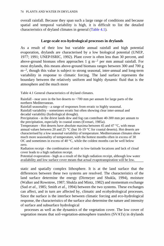
overall rainfall. Because they span such a large range of conditions and becausespatial and temporal variability is high, it is difficult to list the detailedcharacteristics of dryland climates in general (Table 4.1).
Large-scale eco-hydrological processes in drylands
As a result of their low but variable annual rainfall and high potentialevaporation, drylands are characterised by a low biological potential (UNEP,1977; 1991; UNEP/ISRIC, 1992). Plant cover is often less than 30 percent, andabove-ground biomass often approaches 1 g m−2 per mm annual rainfall. Formost drylands, this means above-ground biomass ranges between 300 and 700 gm−2, though this value is subject to strong seasonal, inter-annual and long-termvariability in response to climatic forcing. The land surface represents theboundary between the relatively uniform and highly dynamic fluid that is theatmosphere and the much more
Table 4.1 General characteristics of dryland climates.
Rainfall - near zero in the hot deserts to ~700 mm per annum for large parts of thenorthern Mediterranean.Rainfall seasonality - a range of responses from erratic to highly seasonal.Rainfall variability - sometimes erratic but often showing clear inter-annual anddecadal variability (hydrological drought).Precipitation - in the driest lands dew and fog can contribute 40-300 mm per annum tothe precipitation, especially in coastal zones (Evenari, 1985a).Temperature - Hot deserts have absolute maxima between 45 and 47 “C, with meanannual values between 20 and 25 “C (but 16-19 “C for coastal deserts). Hot deserts arecharacterised by a low seasonal variability of temperature. Mediterranean climates showmuch more seasonality of temperature, with the hottest months often in excess of 30OC and sometimes in excess of 40 “C, while the coldest months can be well belowzero.Radiation receipt - the combination of mid- to low-latitude locations and lack of cloudcover leads to a high radiation receipt.Potential evaporation - high as a result of the high radiation receipt, although low wateravailability and low surface cover means that actual evapotranspiration will be low.
static and spatially complex lithosphere. It is at the land surface that thedifferences between these two systems are resolved. The characteristics of theland surface determine the energy (Dirmeyer and Shukla, 1994), moisture(Walker and Rowntree, 1987; Shukla and Mintz, 1982) and momentum exchange(Sud et al., 1985; Smith et al., 1994) between the two systems. These exchangescan affect, and in turn are affected by, climatic and ecohydrological processes.Since the surface is the interface between climatic forcing and eco-hydrologicalresponse, the characteristics of the surface also determine the nature and intensityof surface and subsurface hydrological
processes as well as the dynamics of the vegetation cover. The low cover ofvegetation means that soil-vegetation-atmosphere transfers (SVATs) in drylands
74 PLANTS AND WATER IN DRYLANDS
are particularly complex (Shuttleworth and Wallace, 1985; Noilhan et al., 1997;Pelgrum and Bastiaanssen, 1996). SVATs in drylands are complicated in two mainways. First, the low and discontinuous vegetation cover presents the atmospherewith a very complex surface when compared with a continuous forest cover orgrassland characteristic of more humid environments. Second, the boundarylayer behaviour of dryland soils and dryland vegetation is quite distinct, and ourunderstanding of hydrological and micrometeorological feedback between the tworemains elementary (see Sene, 1996).
A number of crude general circulation model (GCM) sensitivity experimentsin various ecosystems have suggested that the characteristics of the surface havean important influence on the medium- and long-term dynamics of the climatesystem (Wilson et al., 1987; Meehl and Washington, 1988; Koster and Suarez,1994; Marengo et al., 1994; Eltahir and Bras, 1994; Polcher and Laval, 1994;Stockdale et al., 1994). Most of these experiments have been carried out withinthe context of large-scale field experiments in the same ecosystem (Bolle et al.,1993; Gouturbe et al., 1994). Most of the early experiments of this type dealtwith simple surfaces such as continuous forest cover (Blyth et al., 1994;Shuttleworth et al.,1991) and grassland (Betts et al., 1992; Hall and Sellers,1995). Some of the later experiments considered more complex surfaces such asNorth African crops and tiger-bush (HAPEX-Sahel: Goutorbe et al., 1994),Mediterranean shrublands and rain-fed and irrigated agriculture (Echival FieldExperiment in a Desertification-Threatened Area — EFEDA I and II: Bolle etal., 1993). The early experiments looked at the impact of large-scale changes insurface cover associated with deforestation and afforestation on boundary layerstructure and SVAT fluxes of water, energy and momentum. They were mainlydeforestation experiments (O’Brien, 1996; Sud et al., 1996; Lean and Rowntree,1997). It was clear, numerically and empirically, that these gross changes had asignificant impact on local, regional and, potentially, global climates.
The later experiments looked at much more subtle surface changes associatedwith the progressive reduction of the biological potential of the land in responseto climatic aridification and agricultural intensification. These desertificationexperiments (Gouturbe et al., 1994; Bolle et al., 1993; Xue and Shukla, 1996)produced evidence to support the hypothesised feedback between aridificationand degradation of the land surface. Reduced vegetation cover, higher albedo,lower latent heat loss and higher sensible heat loss result from aridification andlead to less turbulence and cloud formation, in turn causing further aridificationof the climate (Figure 4.1). The most significant characteristics of the vegetationcover in this process are plant albedo (vegetation type, cover, leaf area index),the degree of atmospheric coupling of the stomata (i.e. the degree to whichstomatal opening is controlled by atmospheric variables as opposed to soilmoisture availability; see Chapter 2) and the seasonal phenology of thevegetation cover. Anthropic land-use change in drylands has accelerated in recentdecades and can thus have a direct impact on climate because of this climate—
ECO-HYDROLOGY 75
land-surface properties—climate feedback loop (Henderson Sellers, 1994; Dale,1997).
Plant-soil-water relationships in drylands
The water budget of any part of a dryland hill slope can be expressed as thedifference between water inputs at a point (precipitation, run-on and seepage)and water outputs at the same point (evapotranspiration, runoff and drainage).The most important components of the budget for most drylands are precipitationand evapotranspiration, and so the balance between the two, expressed as theratio of precipitation to potential evapotranspiration, is a good measure ofaridity.
Rainfall
Precipitation in drylands is low in volume, irregular and low in frequency, andoften high in intensity. The irregularity of precipitation can be as important incontrolling plant-soil-water relationships as the long-term mean totalprecipitation, since plants require a constant supply of water for the maintenanceof biological activity, and most species have no way of storing water surpluses.The irregularity of precipitation in drylands can be expressed as the coefficientof variation of annual total precipitation, and this is commonly of the order of 30percent for semi-arid Spain (Mulligan, 1996a), 25 percent for MediterraneanFrance, and around 35 percent in New Mexico (Wainwright, in press, a). In morearid areas, these values are commonly exceeded. Rumney (1968) gives values inexcess of 40 percent for much of the Sudano-Sahelian belt, parts of Mongolia,the southwest coast of Africa and parts of Peru, Bolivia and Argentina.
The characteristics of precipitation in drylands determine to a large extent thehydrological fate of the same precipitation. These characteristics include (1) thetiming of rainfall both seasonally and with respect to previous events; (2) theintensity of rainfall relative to the rate of surface infiltration of water; and (3) thesize and duration of storms along with the pattern of intensity change throughthem. From an analysis of rainfall data collected using an automatic weatherstation (AWS) at Belmonte, central Spain, Mulligan (1996a) found that mostevents are of low intensity, with few of high intensity. The low-intensity eventsefficiently replenish soil water reserves, while high-intensity events providemore water for rapid overland flow. Mulligan (ibid.) also found that the greatmajority of storms are low in volume. Similar patterns were observed in semi-arid New Mexico by Wainwright (in press, a).
Of more importance to the plant-soil-water relationships are the temporalvariations in rainfall receipt. Ecologically, the most significant of these areseasonality and the length of summer drought. Though rainfall seasonality isstrong in drylands, it is most pronounced in mediterranean environmentscharacterised by a cool, wet winter and a hot, dry summer. The strength of
76 PLANTS AND WATER IN DRYLANDS
seasonality varies from year to year (Figure 4.2). Total annual rainfall itselfvaries inter-annually, decadally and in the longer term (Figure 4.3), and
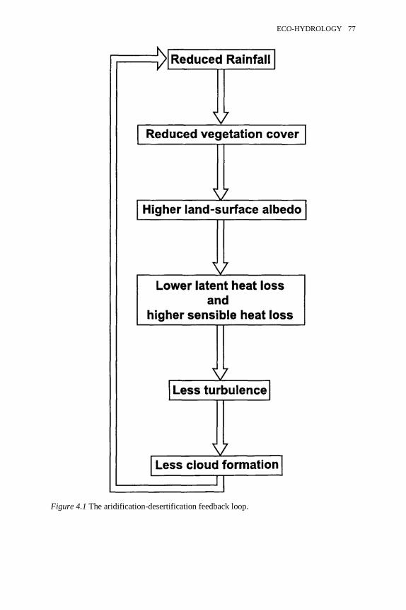
Figure 4.1 The aridification-desertification feedback loop.
ECO-HYDROLOGY 77
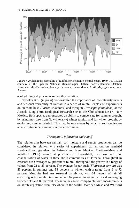
ecohydrological processes reflect this variation.Reynolds et al. (in press) demonstrated the importance of low-intensity events
and seasonal variability of rainfall in a series of rainfall-exclosure experimentson creosote bush (Larrea tridentata) and mesquite (Prosopis glandulosa) at theJornada Long-Term Ecological Research site in the Chihuahuan Desert, NewMexico. Both species demonstrated an ability to compensate for summer droughtby using moisture from (low-intensity) winter rainfall and for winter drought byexploiting summer rainfall. This may be one means by which shrub species areable to out-compete annuals in this environment.
Throughfall, infiltration and runoff
The relationship between rainfall, soil moisture and runoff production can beconsidered in relation to a series of experiments carried out on semiaridshrubland and grassland in Arizona and New Mexico. Martinez-Mesa andWhitford (1996) looked at processes of throughfall, stemflow and rootchannelisation of water in three shrub communities at Jornada. Throughfall increosote bush averaged 56 percent of rainfall throughout the year with a range ofvalues from 22 to 83 percent. The average for tar bush (Flourensia cernua) was53 percent in summer and 58 percent in winter, with a range from 9 to 73percent. Mesquite had less seasonal variability, with 64 percent of rainfalloccurring as throughfall in summer and 62 percent in winter, with values rangingbetween 36 and 89 percent. These values seem comparable with measurementson shrub vegetation from elsewhere in the world. Martinez-Mesa and Whitford
Figure 4.2 Changing seasonality of rainfall for Belmonte, central Spain, 1940–1991. Datacourtesy of the Spanish National Meteorological Office. son=September, October,November; djf=December, January, February; mam=March, April, May; jja=June, July,August.
78 PLANTS AND WATER IN DRYLANDS
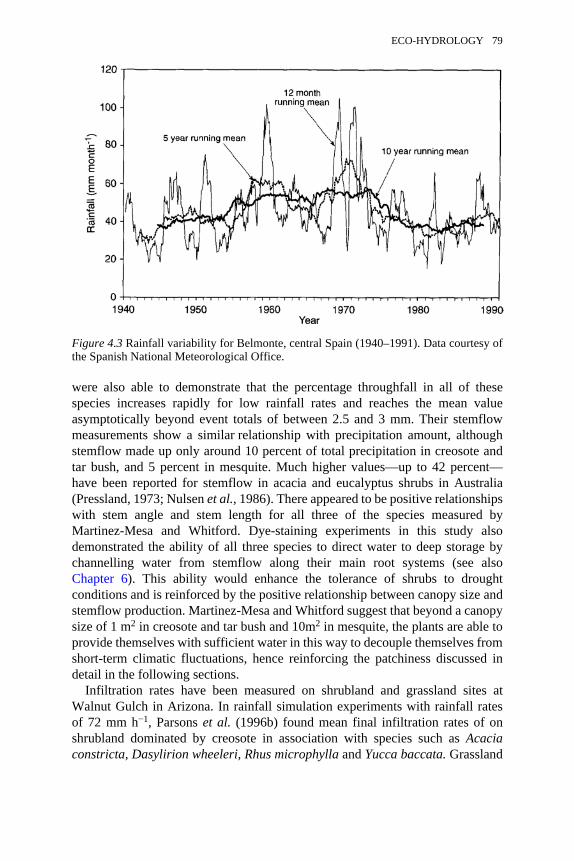
were also able to demonstrate that the percentage throughfall in all of thesespecies increases rapidly for low rainfall rates and reaches the mean valueasymptotically beyond event totals of between 2.5 and 3 mm. Their stemflowmeasurements show a similar relationship with precipitation amount, althoughstemflow made up only around 10 percent of total precipitation in creosote andtar bush, and 5 percent in mesquite. Much higher values—up to 42 percent—have been reported for stemflow in acacia and eucalyptus shrubs in Australia(Pressland, 1973; Nulsen et al., 1986). There appeared to be positive relationshipswith stem angle and stem length for all three of the species measured byMartinez-Mesa and Whitford. Dye-staining experiments in this study alsodemonstrated the ability of all three species to direct water to deep storage bychannelling water from stemflow along their main root systems (see alsoChapter 6). This ability would enhance the tolerance of shrubs to droughtconditions and is reinforced by the positive relationship between canopy size andstemflow production. Martinez-Mesa and Whitford suggest that beyond a canopysize of 1 m2 in creosote and tar bush and 10m2 in mesquite, the plants are able toprovide themselves with sufficient water in this way to decouple themselves fromshort-term climatic fluctuations, hence reinforcing the patchiness discussed indetail in the following sections.
Infiltration rates have been measured on shrubland and grassland sites atWalnut Gulch in Arizona. In rainfall simulation experiments with rainfall ratesof 72 mm h−1, Parsons et al. (1996b) found mean final infiltration rates of onshrubland dominated by creosote in association with species such as Acaciaconstricta, Dasylirion wheeleri, Rhus microphylla and Yucca baccata. Grassland
Figure 4.3 Rainfall variability for Belmonte, central Spain (1940–1991). Data courtesy ofthe Spanish National Meteorological Office.
ECO-HYDROLOGY 79
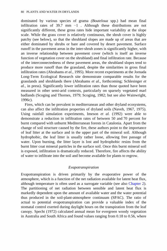
dominated by various species of grama (Bouteloua spp.) had mean finalinfiltration rates of 39.7 mm −1 . Although these distributions are notsignificantly different, these gross rates hide important variability at the slopescale. While the grass cover is relatively continuous, the shrub cover is highlypatchy (see below), so that the shrubland slopes are made up of areas that areeither dominated by shrubs or bare and covered by desert pavement. Surfacerunoff in the pavement areas in the inter-shrub zones is significantly higher, withan inverse relationship between pavement cover (which is itself an inversefunction of vegetation cover on the shrubland) and final infiltration rate. Becauseof the interconnectedness of these pavement areas, the shrubland slopes tend toproduce more runoff than the grassland, despite the similarities in gross finalinfiltration rates (Abrahams et al., 1995). More recent experiments at the JornadaLong-Term Ecological Research site demonstrate comparable results for thegrasslands and shrublands there (Abrahams et al., forthcoming; Schlesinger etal., in press). Significantly lower infiltration rates than those quoted have beenmeasured in other semi-arid contexts, particularly on sparsely vegetated marlbadlands (Scoging and Thornes, 1979; Scoging, 1982; but see also Wainwright,1996c).
Fires, which can be prevalent in mediterranean and other dryland ecosystems,can also affect the infiltration properties of dryland soils (Naveh, 1967, 1975).Using rainfall simulation experiments, Imeson et al. (1992) were able todemonstrate a reduction in infiltration rates of between 50 and 70 percent forburnt compared with unburnt Mediterranean forests in Catalonia. Apart from thechange of soil structure caused by the fire, these authors point to the importanceof leaf litter at the surface and in the upper part of the mineral soil. Althoughhydrophobic, the leaf litter is usually rather loose, allowing free passage ofwater. Upon burning, the litter layer is lost and hydrophobic resins from theburnt litter coat mineral particles in the surface soil. Once this burnt mineral soilis exposed, infiltration is dramatically reduced. Therefore, fire affects the abilityof water to infiltrate into the soil and become available for plants to regrow.
Evapotranspiration
Evapotranspiration is driven primarily by the evaporative power of theatmosphere, which is a function of the net radiation available for latent heat flux,although temperature is often used as a surrogate variable (see also Chapter 2).The partitioning of net radiation between sensible and latent heat flux ismarkedly dependent upon the amount of available water and the water potentialthus produced in the soil-plant-atmosphere continuum (SPAC). The ratio ofactual to potential evapotranspiration can provide a valuable index of thestomatal control exerted during daylight hours on the transpiration from the leafcanopy. Specht (1972) calculated annual mean for evergreen woody vegetationin Australia and South Africa and found values ranging from 0.18 to 0.56, where
80 PLANTS AND WATER IN DRYLANDS
values >0.2 indicate sufficient soil moisture to allow rapid growth of understoreyvegetation.
Because is a measure of stomatal activity it is also a measure of the rate ofpotential photosynthesis. Where is high, stomata are open and photosyntheticactivity and growth rates are high. Stomatal closure reduces CO2 uptake and thusproductivity. The reduced productivity reduces the leaf mass that can bemaintained and thus causes a reduction in the leaf area index, causing reductionsin evapotranspiration. In this way, carbon gain and water loss are locked in a tightfeedback control loop. To model the dynamics of hydrology or plant growth indrylands usefully, one must take account of this feedback and develop coupledhydrology-growth models.
At the drier end of the climatic spectrum, plants are much more stronglycoupled with their hydrological environment, since it is even more marginal interms of their survival. On a continuum of aridity from semi-deserts (300 to 400mm per year) through true deserts (less than 120 mm per year) to extreme deserts(less than 70 mm per year), one can observe distinct changes in the plantcommunity. Tree-like species do not occur where rainfall is below 400 mm,while the 120 mm isohyet is the boundary between steppe (semi-desert) and desertvegetation (Shmida, 1985). The 70 mm isohyet corresponds roughly to theboundary between ‘diffuse’ and ‘contracted’ vegetation. Diffuse vegetation isthat with a low cover (<10 percent) of sparse dwarf shrubs (chamaephytes) and,in the rainy season, a flush of annuals. Contracted vegetation is restricted towadis, where it can take advantage of accumulations of water at depth. At thewetter end of the spectrum, steppe (semi-desert) merges into grassland andshrubland, savannah and woodland. In all of these communities, vegetationcover and plant size are positively correlated with rainfall (Shmida, 1972;Beatley, 1974, 1976). Species diversity is also related to rainfall, with maximumspecies richness occurring in the semi-desert zone between desert and forestecosystems. However, edaphic variability and ecological stability are alsoimportant—ecologically stable areas are thought to have fewer species, thoughthis is highly contentious (Tilman, 1994; Whitford, 1997).
Evenari (1985b) describes the adaptations of plants to the desert environment.He distinguishes the poikilohydrous plants (lichens and algae) and thehomoiohydrous plants. Poikilohydrous plants have a number of physiologicaladaptations to extreme aridity, which are outlined in Table 4.2. Lichens can be avery significant component of dryland vegetation. However, most desert plantsfall into the broad class of homoiohydrous but can be further classified as arido-passive perennials, arido-passive pluviotherophytes, arido-active perennials andbiseasonal annuals. These types possess a number of adaptations to aridity,which are fully described elsewhere (ibid.).
ECO-HYDROLOGY 81
Plant structures and patterns
Spatial structure
Perhaps the most striking characteristic of dryland vegetation is its low cover. Asone moves along a continuum of aridity from down to the potential vegetationcover breaks up from total cover through a series of broken canopies to asituation in which vegetation cover is very patchy. The patches are characterisedby a high density of stems in a small area and a consequent build-up of sediment—typically derived from rain splash or aeolian activity—and organic materialbeneath the vegetation (Parsons et al., 1992; Sánchez and Puigdefábregas, 1994;Puigdefábregas and Sánchez, 1996;
Table 4.2 Features of poikilohydrous plants (after Evenari, 1985b).
1. The capacity to take up water from rain, dew or water vapour in the air (at >70%humidity).
2. The capacity to equilibrate with the hydration level of their environment and tosurvive extreme and prolonged desiccation without damage.
3. The capacity to enter an anabiotic state (with extreme cold and heat resistance) andbecome metabolically inactive after desiccation without injury.
4. Rapid switching on and off of metabolic activity according to water availability.5. Relatively high rate of photosynthesis at low temperatures and low light
intensities.
Wainwright et al., 1995; in press). The resulting increase in surface elevationmay prevent erosion either by diverting overland flow and/or by obstructing theflow and reducing the local slope, leading to an increase in the amounts ofinfiltration of water and deposition of sediment generated on bare patches upslopeof the plants (Cerdà, 1997). This process enhances the soil moisture storage andthe soil moisture storage capacity of the patches at the expense of upslope bareareas. This kind of environmental ‘manipulation’ has been identified in drylandsfrom Israel (Valentine and Nagorcka, 1979) through the Mediterranean to NorthAfrica (Lefever and Lejeune, 1997) and subSaharan Africa (MacFadyen, 1950;Grove, 1957; Worral, I960), as well as in the American southwest (Schlesingeret al., 1990), Patagonia (Rostagno and del Valle, 1988) and Australia (Mabbuttand Fanning, 1987) and can lead to the development of hill-slope-scale, and evenregional, patterned structures on sloping terrain. Dunkerley (1997) has suggestedon the basis of model simulations and evidence from eastern Australia that suchpatterns are relatively stable under, and may even be enhanced by, drought and/or grazing pressure. Davis and Burrows (1994) have also proposed that therepeated occurrence of fires can be an important factor in the development ofvegetation patchiness in drylands.
82 PLANTS AND WATER IN DRYLANDS
Patch development
While a number of plant-scale advantages of clumping can be recognised, theecological mechanism for the phenomenon remains poorly understood, althoughrecent theoretical (van der Maarel, 1988) and modelling (Sánchez andPuigdefábregas, 1994; Puigdefábregas and Sánchez, 1996; Jeltsch et al., 1996)studies have helped in understanding the processes involved. In addition toincreasing the available soil moisture and soil moisture capacity throughoverland flow trapping, clumping can have a number of other ecohydrologicalimpacts, some of which are presented in Table 4.3.
Plant controls on runoff and sediment movement
General considerations
There is a complex and often non-linear interaction between vegetation, hillslopehydrological processes and erosion. Despite this, many forest engineers indrylands still promote the long-held, and somewhat simplistic, idea thatdegradation and soil erosion can be reduced and hydrological processes adjustedby encouraging the growth of forests.
The core of the forest protection approach is based on more than 100 years ofpaired catchment experiments in the USA and the UK and the repeated empiricalobservation that sediment yields are less from forested catchments and well-vegetated plots. A critical review of the confused signals coming
Table 4.3 The eco-hydrological consequences of vegetation clumping.
1. Reduction of soil evaporation loss through shading of the root zone soil.2. Enhancement of root zone moisture supply through the concentration of stemflow.3. Increase of the infiltration or direct rainfall and reduction of overland flow loss.4. Provision of a low air temperature and high-humidity environment around the
majority of leaves, which may reduce transpirational loss.5. Concentration of nutrient reserves in the surface soil from (drought deciduous) leaf
loss, thereby reducing nutrient losses.6. Reduction of grazing pressure by excluding access to all but the edge of the patch.7. Provision of a shaded environment for small animals, enhancing their contribution
to the nutrient budget of the plant and also increasing the potential soil moisturestorage by their burrowing.
8. Reduction of the expenditure on below-ground biomass by bringing resources tothe roots rather than growing roots to the resources.
from this research reveals that the main causes of ambiguity have been thefailure to obtain truly comparable paired catchments, the difficulty engenderedby comparing different serial rainfall inputs to the catchments and the differencesin both treatment and responses of the catchments. In this latter instance, Obando
ECO-HYDROLOGY 83
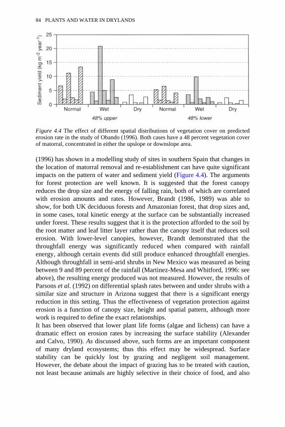
(1996) has shown in a modelling study of sites in southern Spain that changes inthe location of matorral removal and re-establishment can have quite significantimpacts on the pattern of water and sediment yield (Figure 4.4). The argumentsfor forest protection are well known. It is suggested that the forest canopyreduces the drop size and the energy of falling rain, both of which are correlatedwith erosion amounts and rates. However, Brandt (1986, 1989) was able toshow, for both UK deciduous forests and Amazonian forest, that drop sizes and,in some cases, total kinetic energy at the surface can be substantially increasedunder forest. These results suggest that it is the protection afforded to the soil bythe root matter and leaf litter layer rather than the canopy itself that reduces soilerosion. With lower-level canopies, however, Brandt demonstrated that thethroughfall energy was significantly reduced when compared with rainfallenergy, although certain events did still produce enhanced throughfall energies.Although throughfall in semi-arid shrubs in New Mexico was measured as beingbetween 9 and 89 percent of the rainfall (Martinez-Mesa and Whitford, 1996: seeabove), the resulting energy produced was not measured. However, the results ofParsons et al. (1992) on differential splash rates between and under shrubs with asimilar size and structure in Arizona suggest that there is a significant energyreduction in this setting. Thus the effectiveness of vegetation protection againsterosion is a function of canopy size, height and spatial pattern, although morework is required to define the exact relationships. It has been observed that lower plant life forms (algae and lichens) can have adramatic effect on erosion rates by increasing the surface stability (Alexanderand Calvo, 1990). As discussed above, such forms are an important componentof many dryland ecosystems; thus this effect may be widespread. Surfacestability can be quickly lost by grazing and negligent soil management.However, the debate about the impact of grazing has to be treated with caution,not least because animals are highly selective in their choice of food, and also
Figure 4.4 The effect of different spatial distributions of vegetation cover on predictederosion rate in the study of Obando (1996). Both cases have a 48 percent vegetation coverof matorral, concentrated in either the upslope or downslope area.
84 PLANTS AND WATER IN DRYLANDS
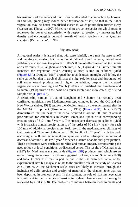
because most of the enhanced runoff can be attributed to compaction by hooves.In addition, grazing may induce better fertilisation of soil, so that in the Sahelvegetation may be better established closer to water points than further away(Warren and Khogali, 1992). Moreover, there are some species for which grazingimproves the cover characteristics with respect to erosion by increasing leafdensity and encouraging outward growth of bushy species such as Quercuscoccifera (Barbero et al., 1990).
Regional scale
At regional scales it is argued that, with zero rainfall, there must be zero runoffand therefore no erosion, but that as the rainfall and runoff increase, the sedimentyield must also increase to a peak at c. 300–500 mm of effective rainfall (i.e. semi-arid environments) (Langbein and Schumm, 1958; Figure 4.5A). Further rainfallincreases the vegetation cover, causing a steep slump in sediment yield(Figure 4.5A). Douglas (1967) argued that total denudation might well follow thesame curve, but that in tropical climates the high solution rates and throughput ofsoil water would produce much higher denudation, despite the increasedvegetation cover. Walling and Webb (1983) also qualified the Langbein andSchumm (1958) curve on the basis of a much greater and more carefully filteredsample size (Figure 4.6). A relationship similar to that of Langbein and Schumm has recently beenconfirmed empirically for Mediterranean-type climates in both the Old and theNew Worlds (Inbar, 1992) and for the Mediterranean by the experimental sites inthe MEDALUS project (Kosmas et al., 1997) (Figure 4.5B). Inbar (1992)demonstrated that the peak of the curve occurred at around 300 mm of annualprecipitation for catchments in coastal Israel and Spain, with correspondingerosion rates of 310 t km−2 year−1. The subsequent decrease in sediment yieldwith increasing annual precipitation is of the order of 50 t km−2 year−1 for each100 mm of additional precipitation. Peak rates in the mediterranean climates ofCalifornia and Chile are of the order of 500 to 600 t km−2 year−1, with the peakoccurring at 400 mm of annual precipitation, and a subsequent more rapiddecrease of around 100 t km−2 year−1 for each 100 mm of additional precipitation.These differences were attributed to relief and human impact, demonstrating theneed to look at local conditions, as discussed below. The results of Kosmas et al.(1997) for Mediterranean shrublands (Figure 4.5B) produce rates which are anorder of magnitude lower than those suggested by Langbein and Schumm (1958)and Inbar (1992). This may in part be due to the less disturbed nature of theexperimental sites but may also relate to the smaller scale of the study of Kosmaset al. (1997). At the catchment scale, rates are likely to increase through theinclusion of gully erosion and erosion of material in the channel zone that hasbeen deposited in previous events. In this context, the role of riparian vegetationis significant in the dynamics of erosion in dryland channels and is thoroughlyreviewed by Graf (1988). The problems of moving between measurements and
ECO-HYDROLOGY 85
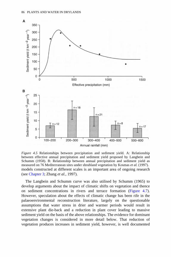
models constructed at different scales is an important area of ongoing research(see Chapter 3; Zhang et al., 1997).
The Langbein and Schumm curve was also utilised by Schumm (1965) todevelop arguments about the impact of climatic shifts on vegetation and thenceon sediment concentrations in rivers and terrace formation (Figure 4.7).However, speculation about the effects of climatic change has been rife in thepalaeoenvironmental reconstruction literature, largely on the questionableassumptions that water stress in drier and warmer periods would result inextensive plant die-back and a reduction in plant cover leading to massivesediment yield on the basis of the above relationships. The evidence for dominantvegetation changes is considered in more detail below. That reduction ofvegetation produces increases in sediment yield, however, is well documented
Figure 4.5 Relationships between precipitation and sediment yield. A: Relationshipbetween effective annual precipitation and sediment yield proposed by Langbein andSchumm (1958). B: Relationship between annual precipitation and sediment yield asmeasured on 76 Mediterranean sites under shrubland vegetation by Kosmas et al. (1997).
86 PLANTS AND WATER IN DRYLANDS
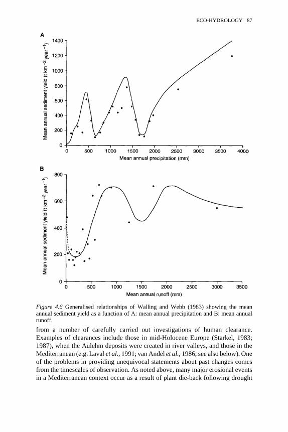
from a number of carefully carried out investigations of human clearance.Examples of clearances include those in mid-Holocene Europe (Starkel, 1983;1987), when the Aulehm deposits were created in river valleys, and those in theMediterranean (e.g. Laval et al., 1991; van Andel et al., 1986; see also below). Oneof the problems in providing unequivocal statements about past changes comesfrom the timescales of observation. As noted above, many major erosional eventsin a Mediterranean context occur as a result of plant die-back following drought
Figure 4.6 Generalised relationships of Walling and Webb (1983) showing the meanannual sediment yield as a function of A: mean annual precipitation and B: mean annualrunoff.
ECO-HYDROLOGY 87
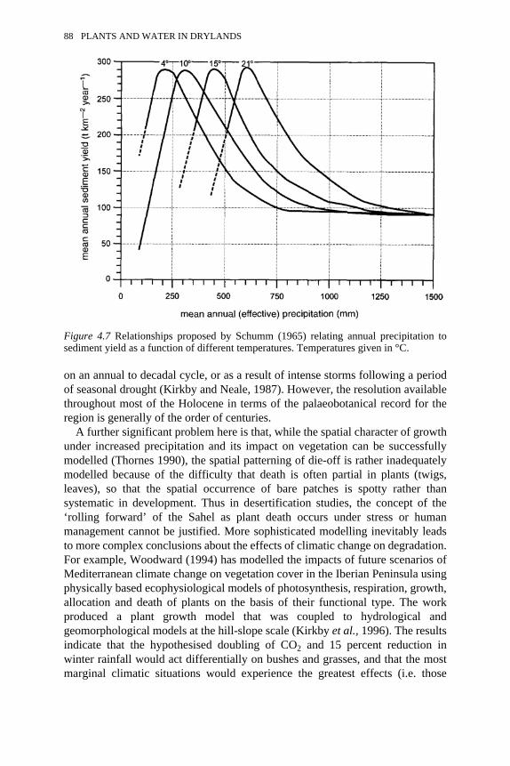
on an annual to decadal cycle, or as a result of intense storms following a periodof seasonal drought (Kirkby and Neale, 1987). However, the resolution availablethroughout most of the Holocene in terms of the palaeobotanical record for theregion is generally of the order of centuries.
A further significant problem here is that, while the spatial character of growthunder increased precipitation and its impact on vegetation can be successfullymodelled (Thornes 1990), the spatial patterning of die-off is rather inadequatelymodelled because of the difficulty that death is often partial in plants (twigs,leaves), so that the spatial occurrence of bare patches is spotty rather thansystematic in development. Thus in desertification studies, the concept of the‘rolling forward’ of the Sahel as plant death occurs under stress or humanmanagement cannot be justified. More sophisticated modelling inevitably leadsto more complex conclusions about the effects of climatic change on degradation.For example, Woodward (1994) has modelled the impacts of future scenarios ofMediterranean climate change on vegetation cover in the Iberian Peninsula usingphysically based ecophysiological models of photosynthesis, respiration, growth,allocation and death of plants on the basis of their functional type. The workproduced a plant growth model that was coupled to hydrological andgeomorphological models at the hill-slope scale (Kirkby et al., 1996). The resultsindicate that the hypothesised doubling of CO2 and 15 percent reduction inwinter rainfall would act differentially on bushes and grasses, and that the mostmarginal climatic situations would experience the greatest effects (i.e. those
Figure 4.7 Relationships proposed by Schumm (1965) relating annual precipitation tosediment yield as a function of different temperatures. Temperatures given in °C.
88 PLANTS AND WATER IN DRYLANDS
areas having an average dry season of seven months without rain). The resultsindicate losses in biomass of up to 50 percent, which would be expected toproduce a dramatic change in sediment yield.
Slope or plot scale
At smaller scales, variability in the controls of erosion such as vegetation leads tomuch greater spatial and temporal variability in rates. For this reason, local-scaleestimates of erosion must be based on a thorough understanding of the processes.The erosion process can be divided into three interacting elements. Erosion bysplash occurs due to the impact of raindrops on the surface, which can entrainparticles in droplets that rebound from the surface. Once overland flow isgenerated, it can transport sediment either in a rather diffuse manner in theundissected inter-rill zone or in a more concentrated way once incision leads tothe formation of rills and, ultimately, gullies.
Erosion by splash
The splash mechanism is effective for soil particles less than about 12 mm inmaximum dimension (Wainwright, 1992; Wainwright et al., 1995). Transportdistances are typically less than a metre and decline exponentially in all directionsfrom the source although with a net downslope movement (Savat and Poesen,1981). Parsons et al. (1994) demonstrated using rainfall simulations that splashrates increased and then decreased during a first rainfall event on a semi-aridgrassland plot at Walnut Gulch, with peak rates of . During a second eventcarried out three days later, the rates continued to decline. This pattern wasinterpreted as relating initially to the increased wetting of the soils, facilitatingtheir movement by reducing cohesion, followed by a subsequent decrease inavailable soil for transport. Thus, the importance of splash might be expected todecrease, ceteris paribus, during the period of a rainy season at a particular site.As noted below, there is an important interaction between splash and sparsevegetation canopies in drylands. Soil and litter can commonly be splashedunderneath a shrub canopy, but the splash process is considerably reducedbeneath the canopy because of the relatively small proportion of throughfall (seeabove), and thus little material is splashed back out into the inter-shrub areas.Through time, this build-up of soil and litter contributes significantly to theformation of mounds (Parsons et al., 1992; Wainwright et al., 1995; in press).The rapidity with which this occurs is partly a function of splash rates in theinter-shrub areas, which can be an order of magnitude higher than those in thegrassland areas (Parsons et al., 1991).
ECO-HYDROLOGY 89
Erosion by inter-rill overland flow
Overland flow in the inter-rill zone is able to move larger particles— Abrahamset al. (1988) observed movement of particles as large as 53 mm on steep slopes—typically for much greater distances than the splash process. Tracer experimentson the Walnut Gulch grassland suggested that although a large proportion ofmaterial is redeposited within 25 cm of its origin, travel distances of almost 3 mwere recorded in a single event, again with an exponential decline in the amountof material transported with distance (Parsons et al., 1993). These experimentssuggest that the transport is intermittent and that it would take a number ofevents for soil particles to travel the length of the slope and enter the channelsystem. Abrahams et al. (1991) demonstrated that inter-rill erosion is determinedby sediment detachment by raindrops, as the flows themselves have insufficientenergy to detach soils. The capacity to transport such detached material is thendefined by the flow depth, which is itself highly variable due to the significantsurface irregularities on typical dryland slopes (Abrahams and Parsons, 1991;Parsons et al., 1994; 1996a). Raindrop detachment is itself a negativeexponential function of flow depth (Torri et al., 1981), leading to thedevelopment of spatial patterns of erosion. On both the grassland and shrublandslopes at Walnut Gulch, the erosion first increases from the slope divide as flowtransport capacity increases, and then decreases as the raindrop detachmentdecreases, because of the general downslope increase of flow depth (Abrahamset al., 1991; Parsons et al., 1996a). In both cases, there are feedbacks betweenthe vegetation, flow dynamics and erosion. On the shrubland, the high surfacerunoff from the inter-shrub areas increases the erosion in these areas, whichaccentuates the relief of the shrub-topped mounds and equally reduces thelikelihood of recolonisation of the inter-shrub areas, because of the removal ofwater and nutrient resources (Parsons et al., 1996b; Schlesinger et al., in press).The grassland is characterised more by a negative feedback wherein the morediffuse distribution of grass clumps causes overland flow to be slower and lessconcentrated. Sediment is thus deposited behind the clumps, often forming aseries of microtopographic steps, which in turn enhance the diffusion of theoverland flow (Parsons et al., 1996a). Thus, despite the lower vegetation coveron the grassland (33 percent compared with 44 percent on the shrubland), erosionrates are lower, with peak rates of 0.23 g m−2 s−1 compared with 0.53 g m−2 s−1
on the shrubland. It can be seen that inter-rill overland flow is several orders ofmagnitude more effective at transporting sediment than splash (see alsoWainwright, 1996b and c for Mediterranean examples).
Erosion by concentrated overland flow
Erosion in concentrated overland flow occurs when the flow gains sufficientenergy to detach sediment itself, thus causing incision into the soil surface,forming rills and ultimately gullies. In this case, the detachment of soil by
90 PLANTS AND WATER IN DRYLANDS
raindrops is no longer a limiting factor. Rilling occurs on the shrubland atWalnut Gulch and is apparently controlled by the occurrence of greater extremesof flow depth in the downslope direction (Parsons et al., 1996a). This is probablya further consequence of the feedback described above, where flow isincreasingly constrained into the inter-shrub areas as it travels downslope.Unpublished work at the Jornada site suggests that shrub spacing is a dominantcontrol on this process (Charlton, personal communication).
The example discussed in detail above suggests that simple models that showa negative exponential relationship between vegetation cover and erosion—as,for example, demonstrated by Elwell and Stocking (1976) for simple crops—cannot be said to hold in all cases in drylands. Rogers and Schumm (1991) havealso shown experimentally that the negative exponential relationship breaksdown at vegetation covers of 15 percent or less. Morgan (1996) has discusseddifferences in the form of the relationship and its parameters in relation tocanopy structure as part of the European Soil-Erosion Model (EUROSEM)project. It would appear that further work on this problem is required that takesaccount of the canopy structure of dryland plants and their spatial distribution ona slope. Given that many drylands have plant covers of less than 30 percent, asnoted above, this point is of critical importance.
As with runoff production, the consequences of fire are an importantconsideration in relation to erosion, principally because of the increase in runoffdescribed above, the decrease in protection of the soil surface by the vegetationcanopy, and changes in the soil structure. Vega and Diaz Fiernos (1987) showeda difference of erosion rates, with only 1.5 t ha−1 year−1 produced on amoderately burnt Pinus pinaster woodland, compared with 22 t ha−1 year−1 on anintensely burnt area in northwest Spain. On Quercus ilex plots in Catalonia,Soler and Sala (1992) measured erosion rates of 0.017 t ha−1 year−1 on unburntand 0.162 t ha−1 year−1 on burnt plots, compared with 0.024 t ha−1 year−1 wherethe plots had simply been cleared. Fire can also lead to a loss of nutrients fromthe system by a number of mechanisms (Christensen, 1994), which, combinedwith soil loss, has important consequences for vegetation regrowth (Soler andSala, 1992; Kutiel and Inbar, 1993).
MODELLING ECO-HYDROLOGICAL PROCESSES INDRYLANDS
Models for understanding dryland eco-hydrology
Numerical models (see Chapter 9) are increasingly being used as an aid to fieldexperimentation and theoretical analysis for understanding the eco-hydrologicaldynamics of drylands. Models are applied at scales from the GCM grid cell, suchas the land-surface sensitivity experiments discussed above and in Chapter 3,through to the individual plant scale. Models are applied for time periods from a
ECO-HYDROLOGY 91
few hours for process studies and event simulation through to hundreds of yearsfor climate change experiments. A number of hydrological (for example, Braudet al., 1995, Kirkby and Neale, 1987, Kirkby, 1990), ecological (for example,MARIOLA, Uso-Domenech et al., 1995) and coupled eco-hydrological models(for example, PATTERN, Mulligan, 1996a and b; MEDALUS, Kirkby et al.,1996; FOREST-BGC, Kremer et al., 1996; Thornes, 1990) have been developedfor dryland environments.
The particular characteristics of dryland climates, surfaces and plantcommunities require a particular set of modelling strategies appropriate to theseconditions.
Model timesteps
Drylands are characterised by long periods of hydrological inactivity with short,intensive events in which a great deal of change occurs. In modelling terms, thisrequires the specification of a high-resolution timestep (perhaps a minute or less)in order to represent accurately rapid rate processes (particularly Hortonianoverland flow) during an extreme event but also low-resolution timesteps forintegration of fluxes outside these periods of activity. In this way, a variabletimestep rather than a fixed one is most appropriate to dryland eco-hydrologicalmodelling. The timestep should respond to the rate of the most rapid acting fluxor process so that it is inversely proportional to this rate. A variable timestep iscomputationally efficient and hydrologically precise.
Where ecological processes are coupled with hydrological ones, andparticularly where processes of the energy budget are included, an additional,concurrent, timestep is required. The timestep should reflect the slower biologicalprocesses and is commonly of the order of hours or days. Hourly timesteps havethe advantage of increased precision but require hourly data, which are often notavailable. Daily timesteps, on the other hand, are easier to parameterise but canlead to significant error because they do not take into account the significantdifferences between daytime processes and night-time processes. These can beparticularly important in drylands, where dew inputs can be high during the nightand where water stress changes significantly between day and night. Theanalysis in Table 4.4 is the result of an application of the Penman-Monteithequation (Monteith, 1973) to the same data set, which is integrated first on anhourly basis, second on a daily basis, and third on a day-night basis with onetimestep from sunrise to sunset and the next timestep from sunset to thefollowing sunrise. Clearly, there are significant differences in the calculatedevapotranspiration between these situations. If we take the hourly results as thosethat most closely represent reality, it is clear that a day-night timestepsignificantly improves the accuracy of estimation of evapotranspiration whencompared to a daily timestep. The accuracy of using the day-night timestep alsovaries through the year, as indicated by the June figures compared with those forJanuary.
92 PLANTS AND WATER IN DRYLANDS
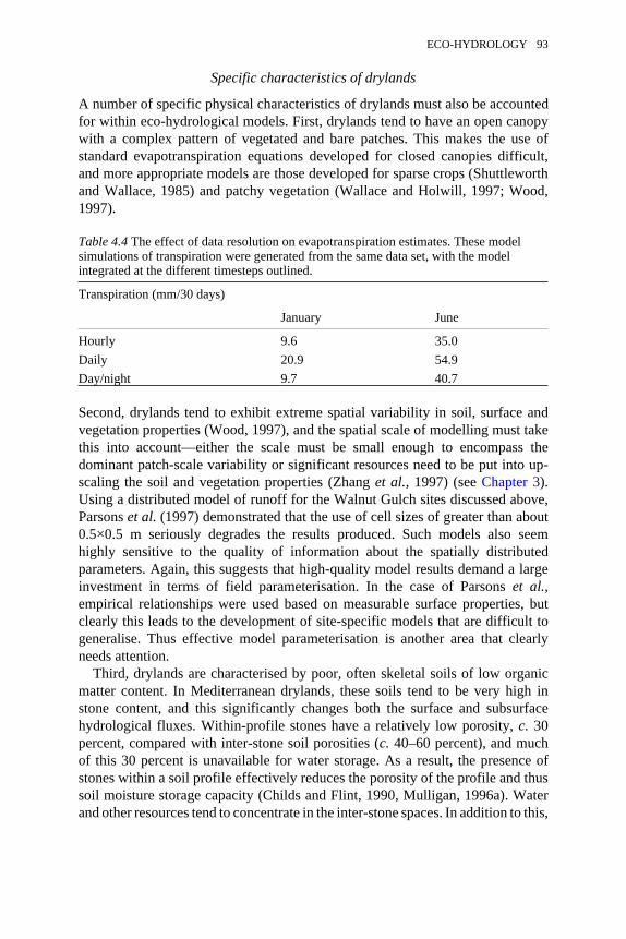
Specific characteristics of drylands
A number of specific physical characteristics of drylands must also be accountedfor within eco-hydrological models. First, drylands tend to have an open canopywith a complex pattern of vegetated and bare patches. This makes the use ofstandard evapotranspiration equations developed for closed canopies difficult,and more appropriate models are those developed for sparse crops (Shuttleworthand Wallace, 1985) and patchy vegetation (Wallace and Holwill, 1997; Wood,1997).
Table 4.4 The effect of data resolution on evapotranspiration estimates. These modelsimulations of transpiration were generated from the same data set, with the modelintegrated at the different timesteps outlined.
Transpiration (mm/30 days)
January June
Hourly 9.6 35.0Daily 20.9 54.9Day/night 9.7 40.7
Second, drylands tend to exhibit extreme spatial variability in soil, surface andvegetation properties (Wood, 1997), and the spatial scale of modelling must takethis into account—either the scale must be small enough to encompass thedominant patch-scale variability or significant resources need to be put into up-scaling the soil and vegetation properties (Zhang et al., 1997) (see Chapter 3).Using a distributed model of runoff for the Walnut Gulch sites discussed above,Parsons et al. (1997) demonstrated that the use of cell sizes of greater than about0.5×0.5 m seriously degrades the results produced. Such models also seemhighly sensitive to the quality of information about the spatially distributedparameters. Again, this suggests that high-quality model results demand a largeinvestment in terms of field parameterisation. In the case of Parsons et al.,empirical relationships were used based on measurable surface properties, butclearly this leads to the development of site-specific models that are difficult togeneralise. Thus effective model parameterisation is another area that clearlyneeds attention.
Third, drylands are characterised by poor, often skeletal soils of low organicmatter content. In Mediterranean drylands, these soils tend to be very high instone content, and this significantly changes both the surface and subsurfacehydrological fluxes. Within-profile stones have a relatively low porosity, c. 30percent, compared with inter-stone soil porosities (c. 40–60 percent), and muchof this 30 percent is unavailable for water storage. As a result, the presence ofstones within a soil profile effectively reduces the porosity of the profile and thussoil moisture storage capacity (Childs and Flint, 1990, Mulligan, 1996a). Waterand other resources tend to concentrate in the inter-stone spaces. In addition to this,
ECO-HYDROLOGY 93
the surface area of pore space at the soil-bedrock interface is reduced by thepresence of stones, and this can reduce the areal rate of recharge to the bedrock.Finally, stones within the soil profile may support the soil structure and in thesecases, or in cases where there is significant diurnal and seasonal temperaturefluctuation, the soil may become removed from the stone surfaces, providing apreferential flow path through the stone ‘skeleton’. These effects have beenexperimentally tested (Childs and Flint, 1990) and modelled (Mulligan, 1996a).
The stone content at the soil surface is a function of the profile stone contentand the rate of removal of surface sediment. Surface stones in drylands havebeen widely studied in the field and laboratory (Poesen, 1986; de Lima and deLima, 1990; Poesen et al., 1990; Poesen and Bunte, 1995) and their hydrologicaleffects modelled (Mulligan, 1996a). They have a significant effect onhydrological fluxes, on the surface energy budget and on the development of thevegetation cover. The two basic hydrological impacts of stones concerninfiltration and soil evaporation. The presence of surface stones effectively sealsa proportion of the surface from infiltration since some of the soil pore space atthe surface is covered by an impermeable stone. This means that during a rainfallevent, water falling on the stone-covered parr runs off as stone flow onto the barepart of the soil. This increases the rare at which water is delivered to the inter-stone soil surface by an amount that is proportional to the stone-soil area ratio. A50 percent cover of stones (common for large areas of the semi-naturalMediterranean shrublands and very common in the desert-pavement-coveredinter-shrub areas of the American southwest) effectively doubles this rate ofwater delivery during rainfall. This can lead to high overland flow generation,leading to enhanced erosion of the inter-stone spaces and removal of soil toexpose further stone surfaces. The importance of this mechanism depends uponwhether the stones are simply resting on the soil surface or whether they arepartly buried within the soil. Stones resting on the surface will tend to leak rainfallinro the underlying pore space and will reduce surface sealing and raindropimpact, thereby potentially increasing infiltration and reducing overland flow,whereas embedded stones tend to have the opposite effect (for a more detailedreview, see Baird, 1997).
Both types of surface stone cover prevent energy from reaching the soil porespace and as such act as a mulch preventing soil evaporation. This can lead to thedevelopment of ecologically important surface wet patches under high stonecovers. Where the vegetation cover is low, a high stone cover can lead toextremely low soil evaporation even from wet soils, but where vegetation coveris high this mechanism is ineffectual since an alternative route for evaporation ispresent through the plants.
94 PLANTS AND WATER IN DRYLANDS
DRYLAND ECO-HYDROLOGY IN SPACE AND TIME
Evolution of plant cover
The first development of plants currently associated with the Mediterraneanregion occurred during the Pliocene. In the eastern Mediterranean, there isevidence from Israel that the Pliocene vegetation was characterised by a cool,temperate woodland (Horowirz and Horowitz, 1985). In the later part of thePliocene, tree cover decreased, being made up of Pinus, Abies orientalisand later Quercus with a dominance of steppe species in sites in the south of thecountry from about 3.5 Ma, suggesting the onset of environmental gradientssimilar to those of the present day (Levin and Horowitz, 1987). Before 3.2 Ma,the northwestern part of the Mediterranean had been characterised by tropicalvegetation species such as Taxodium, Myrica, Symptoms and Nyssa in thelowlands, suggesting high moisture conditions, and lower moisture conditions inthe uplands, as demonstrated by species such as Engelhardia, Carya, Rhioptelea,Hammamelis and Embolanthera (Sue, 1984). Similar associations are found frombefore the Messinian salinity crisis, suggesting a great stability in this pattern(Sue and Bessais, 1990). Mediterranean evergreen and pine species are present inthe early Pliocene in southern Italy between 4.5 and 3.2 Ma, and few tropicalspecies were found (Bertoldi et al., 1989). However, the period from 2.6 to 2.2Ma is marked by cyclic changes in vegetation groupings, with deciduous forest,tropical humid forest, coniferous forest and steppe vegetation all present(Combourieu-Nebout, 1993). Rare Taxodiaceae and subtropical species are stillpresent in the Villafranchian type area of northern Italy between 2.9 and 2.2 Ma(Carraro et at., 1996). The latter part of this sequence and those of southernFrance from 2.3 Ma show an increase of steppe species (Sue and Zagwijn,1983). From 2.1 to 1.7 Ma, the first fully Mediterranean-type vegetation zonationis found in southern France. This is made up of Olea and Ceratonia withPistacia, Phillyrea and Myrtus at the lowest altitudes; Phillyrea and Quercus ilexwith Olea, Carpinus orientalis and Rhamnus at middle altitudes; deciduous oakand Carpinus with Carya, Ulmus and Zelkova at higher altitudes; and finallyCedrus, Pinus, Abies, Picea and Tsuga making up a mountain forest (Sue, 1984).In southern Italy and Sicily, the same period sees the final disappearance of thesubtropical Taxodiaceae (Baggioni et al., 1981; Bertoldi et al., 1989), althoughthey are still present in Calabria (Combourieu-Nebout, 1993) and as late as 1.3Ma in central Italy (Rosa Attolini et al., 1988), albeit most probably as relictpopulations in local refugia.
Thus, the major lines of the modern vegetation show a complex developmentover a period of two million years. The development seems to occur earlier in theeast and south than in the west and north. On the general trend are superimposeda number of cycles of vegetation change. The period of time over which thesechanges occurred is marked by important climate changes within the region thatalso reflect broader global changes. Oxygen isotope data for the western
ECO-HYDROLOGY 95
Mediterranean suggest that temperatures were up to 3 °C higher than presentuntil 3.2 Ma (Thunell, 1979) or 3.1 Ma (Vergnaud-Grazzini et al., 1990), whenthere was a relatively sudden drop in winter sea surface temperatures of 1.2 °C(Keigwin and Thunell, 1979). This change represents the global onset of coolingand sea level fall as seen in the Pacific (Shackleton and Opdyke, 1977) andAtlantic (Clemens and Tiedemann, 1997). A second phase of cooling occurredaround 2.5 Ma, with oscillations until around 2.1 or 2.0 Ma, after which there wasa general downward trend in temperatures until the onset of the larger-scaleglacial-interglacial cycles around 900 ka (Vergnaud-Grazzini et al., 1990;Thunell, 1979; Thunell and Williams, 1983). Estimated sea surface temperaturesfor the period from 2 to 1 Ma range from values similar to those of the presentday to 2 °C higher than at present (Thunell, 1979). Data for the reconstruction ofthe moisture regime independently of the vegetation are much more tenuous.Vergnaud-Grazzini et al. (1990) have suggested that the later Pliocene wasmarked in the Tyrrhenian basin by the gradual onset of a seasonally contrastedrainfall pattern. This was superimposed on conditions that were already relativelydry. Such dry conditions may be reflected by the vegetation associations in Italyand Israel recorded during this period. If this is the case, it may be that thedevelopment of the Mediterranean associations are related to the development ofhighly seasonal water regimes at the same time as the relatively slighttemperature changes experienced. The adaptation of Mediterranean species suchas Quercus ilex to seasonal drought has been noted by a number of authors (e.g.Quézel, 1978; Daget, 1980; Terradas and Savé, 1992; Acherar and Rambal, 1992).Furthermore, the ability of species such as Quercus ilex to control microclimatesand therefore accompanying understorey plants (Barbero et al., 1992) may haveplayed an important part in the selection of the species that now make upMediterranean associations.
The origins of Saharan vegetation are discussed by Maley (1980). Thedevelopment of the Sahara itself took place from the early Pliocene, around 5Ma. Later Pliocene samples from the Hoggar and from Egypt suggest that mostof the elements of the modern vegetation were in place by this time, although theperiod saw the presence of a larger number of tree species than are now found evenin the Hoggar uplands. Le Houérou (1997) suggests that during the various wetterperiods of the Quaternary, the Sahara was an important refuge for Mediterranean-type plants. In East Africa, the initial development of dryland vegetation tookplace in the later Miocene as a consequence of uplift, which caused thedevelopment of large rain shadow areas (van Zinderen Bakker, 1983). Thedevelopment of savannah seems to have taken place here between 2 and 1.8 Ma.
A relatively continuous vegetation sequence covering the last 3 Ma in northernCalifornia is recorded at Tulelake (Adam et al., 1989). Vegetation cover isdominated here by forest with Pinus, Taxodiaceae, Cupressaceae, Taxaceae(TCT) and oak, again representing relatively wet conditions. Around 2.9 andespecially 2.5 Ma, there are fluctuations in the cover with the expansion ofspecies such as Artemisia and desert shrubs. From c. 1.65 Ma, there are a series
96 PLANTS AND WATER IN DRYLANDS
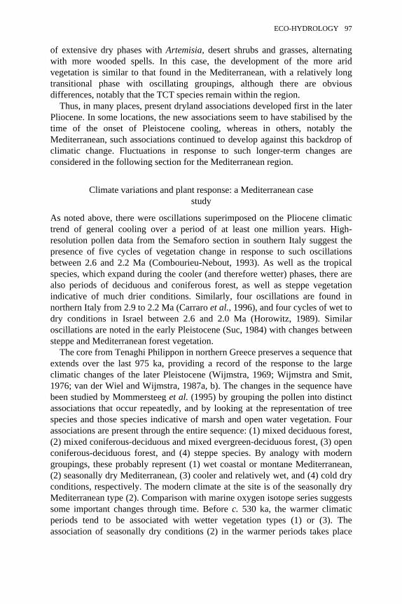
of extensive dry phases with Artemisia, desert shrubs and grasses, alternatingwith more wooded spells. In this case, the development of the more aridvegetation is similar to that found in the Mediterranean, with a relatively longtransitional phase with oscillating groupings, although there are obviousdifferences, notably that the TCT species remain within the region.
Thus, in many places, present dryland associations developed first in the laterPliocene. In some locations, the new associations seem to have stabilised by thetime of the onset of Pleistocene cooling, whereas in others, notably theMediterranean, such associations continued to develop against this backdrop ofclimatic change. Fluctuations in response to such longer-term changes areconsidered in the following section for the Mediterranean region.
Climate variations and plant response: a Mediterranean casestudy
As noted above, there were oscillations superimposed on the Pliocene climatictrend of general cooling over a period of at least one million years. High-resolution pollen data from the Semaforo section in southern Italy suggest thepresence of five cycles of vegetation change in response to such oscillationsbetween 2.6 and 2.2 Ma (Combourieu-Nebout, 1993). As well as the tropicalspecies, which expand during the cooler (and therefore wetter) phases, there arealso periods of deciduous and coniferous forest, as well as steppe vegetationindicative of much drier conditions. Similarly, four oscillations are found innorthern Italy from 2.9 to 2.2 Ma (Carraro et al., 1996), and four cycles of wet todry conditions in Israel between 2.6 and 2.0 Ma (Horowitz, 1989). Similaroscillations are noted in the early Pleistocene (Suc, 1984) with changes betweensteppe and Mediterranean forest vegetation.
The core from Tenaghi Philippon in northern Greece preserves a sequence thatextends over the last 975 ka, providing a record of the response to the largeclimatic changes of the later Pleistocene (Wijmstra, 1969; Wijmstra and Smit,1976; van der Wiel and Wijmstra, 1987a, b). The changes in the sequence havebeen studied by Mommersteeg et al. (1995) by grouping the pollen into distinctassociations that occur repeatedly, and by looking at the representation of treespecies and those species indicative of marsh and open water vegetation. Fourassociations are present through the entire sequence: (1) mixed deciduous forest,(2) mixed coniferous-deciduous and mixed evergreen-deciduous forest, (3) openconiferous-deciduous forest, and (4) steppe species. By analogy with moderngroupings, these probably represent (1) wet coastal or montane Mediterranean,(2) seasonally dry Mediterranean, (3) cooler and relatively wet, and (4) cold dryconditions, respectively. The modern climate at the site is of the seasonally dryMediterranean type (2). Comparison with marine oxygen isotope series suggestssome important changes through time. Before c. 530 ka, the warmer climaticperiods tend to be associated with wetter vegetation types (1) or (3). Theassociation of seasonally dry conditions (2) in the warmer periods takes place
ECO-HYDROLOGY 97
only after this time, which may reflect climate changes due to the shift in theEarth’s orbital activity after c. 600 ka. Even so, it is still relatively infrequent,making up only one-fifth of the total period. Thus, although we have seen thatthe species making up this association in the Mediterranean were in place sincethe Pliocene, the conditions that have led to their full development are relativelyrecent. Dry conditions have more commonly been associated with open, steppevegetation (often with Artemisia, as currently found in the higher Mediterraneanmountains and the arid zones of North Africa: Le Houérou, 1986). From the totalsequence of 975 ka, this association is present for 400 ka. Mommersteeg et al.(1995) demonstrated the presence of orbital frequencies relating to precessionand obliquity effects, which they interpreted as being due to movements in theinter-tropical convergence zone (ITCZ) causing rainfall changes within theMediterranean basin. Horowitz (1989) also postulated the existence of monsoon-related changes in the Pleistocene oscillations between Mediterranean woodlandand steppe in the long sequences from Israel.
Further interesting observations about the longer-term response to climatechange can be obtained by analysis of the changes between the differentvegetation associations outlined by Mommersteeg et al. A Markov chain analysisof these transitions shows a number of patterns of change through time(Figure 4.8). The mixed Mediterranean forest indicative of seasonally dryconditions (2) occurs only after the presence of the deciduous forest (1) or openforest (3). This suggests that wetter conditions are characteristic of transitionalphases, and that such conditions are necessary to produce a substrate upon whichthe mixed forest can be competitive once drier conditions are re-established. Thesteppe vegetation can follow the mixed Mediterranean forest, showing that thereverse process is not necessarily true, although it is slightly more common tohave a transitional open forest phase before steppe conditions fully develop.Another long sequence from Ioannina in northern Greece shows similar stages ofdevelopment at a higher resolution (Tzedakis, 1994). Over the last 423 ka, therehave been nine forested phases, which show a similar pattern of development.Quercus and Ulmus/Zelkova develop early after warming, followed by Carpinusbetulus, C. orientalis and Ostrya carpinifolia and finally Abies, which is oftenaccompanied by Fagus. Species such as Olea, Buxus and Juniperus tend to becommon throughout, albeit in small quantities. The intervening cold periods aremarked by an initial steppe with Graminae, Chenopodiaceae and Artemisia, adesert-steppe with dominant Artemisia and a variety of shrub species, and asteppe-forest transition with rapidly increasing Pinus and Quercus. Similarpatterns have also been observed in long sequences from Italy (Follieri et al.,1988; Watts et al., 1996) and Spain (Pons and Reille, 1988).
The data from Tenaghi Philippon and Ioannina suggest that the Mediterraneanmixed forest vegetation as we see it today is a relatively recent phenomenon.Although a general succession is demonstrated at Ioannina, there may be aninherent instability due to the lateness and infrequency of occurrence of suchassociations. Their vulnerability to disturbance is discussed below.
98 PLANTS AND WATER IN DRYLANDS
Anthropic effects on dryland plants
Following the development of the deciduous then mixed Mediterranean forest inthe late Pleistocene and early Holocene, it becomes increasingly difficult toderive climate-induced change in the region (e.g. Vernet and Thiébault, 1987).By around 6 ka, indeed, it seems difficult to find clear evidence of subsequentclimate change in the European Mediterranean because of the importance ofinter-annual variability (Wainwright, 1996a). This is consistent withpalaeoclimate reconstructions (Guiot, 1987; COHMAP members, 1988; Pons etal., 1992) and GCM experiments (Wright et al., 1993). More humid conditionsseem to have been in place in the northern Sahara until 3297–1776 BC (e.g.Gasse et al., 1987), and some mediterranean species are found with more aridspecies in Sudan as late as 4220–3124 BC* (Ritchie et al., 1985). Followingthese times (and indeed before), we must therefore look to human influence asbeing a dominant cause of vegetation change.
Human activity has caused vegetation to be altered in three ways, each withdistinct hydrological consequences. These ways may be classified as direct,indirect and inadvertent.
(1) deciduous forest: warm, wet Mediterranean 0.57 (2) mixed forest: warm, dryMediterranean 0.07 0.56 (3) open forest: cooler, wet throughout year 0.08 (4)steppe: cold, dry
Figure 4.8 Markov transition probabilities of transitions of vegetation types observed inthe Tenaghi Philippon core. Vegetation types and their timing defined after Mommersteeget al. (1995).
ECO-HYDROLOGY 99
Direct modification of species assemblage
Direct modifications occur either by clearance and deforestation or by deliberateplanting or introduction. Widespread clearance is suggested from pollenevidence, for example in Attica, by 4072–3541 BC (Turner and Greig, 1975) andpossibly even slightly earlier in northern Greece (Willis, 1994). The impact offorest clearance is described above. Deforested landscapes in the northwesternMediterranean led to a number of erosional phases in the second millennium BC(Wainwright, in press, b). Similar phases are recorded in the Argolid in southernGreece in the third millennium BC (Pope and van Andel, 1984) and as early asthe mid-sixth millennium BC in Macedonia (van Andel et al., 1990). Suchepisodes are indicative of greater runoff and possibly also greater recharge intoalluvial aquifers, which may also have affected the development of riparianvegetation. The runoff and erosion may have been accentuated by the use of fireas a means of vegetation clearance, which has a long history in the region(Naveh, 1975).
Deliberate planting includes not only cereals, with consequences for runoffproduction, especially during the period after harvest when the ground surface isrelatively bare and usually crusted, but also vines, olives and other tree crops.Peaks in vine and olive cultivation occur in the mid-second millennium BC,during the first millennium BC, and from the early Mediaeval period(Wainwright, 1997, after Andrieu et al., 1995). Vine cultivation can lead toincreased runoff generation due to the presence of bare areas between the crops(Wainwright, 1996b), although this may have been reduced in the past with moretraditional cultura promiscua techniques, in which tree crops were interplantedwith wheat or legumes, providing a more extensive ground cover. On the otherhand, olive cultivation, particularly with the development of terraces from thethird millennium BC in the Levant and slightly later in southern Greece (vanAndel and Runnels, 1987), may have been important in reversing the processes ofrunoff and sediment production, and the development of irrigation would havehad important effects on the hill-slope hydrology. Indeed, Kosmas et al. (1997)have presented figures for average soil losses from experimental plots of 0.008 tha−1 year−1 under olive cultivation, compared with 1.43 t ha−1 year−1 under vines,0.18 t ha−1 year−1 under wheat and 0.07 t ha−1 year−1 for shrubland. Other treecrops such as chestnut and walnut, which spread in the later first millennium BC(Andrieu et al., 1995), may have had a similar effect even without terracecultivation. Tree crops such as almond, which spread into Spain during theRoman or Moorish period, are unfortunately undetectable by pollen analysis
* These dates and those that follow are calibrated radiocarbon dates given as 2σ ranges, sothat the true date has a 95 percent probability of falling within the given interval.Calibration is according to the program CALIB 3.0 of Stuiver and Reimer (1993), usingthe data of Stuiver and Pearson (1993) and Pearson and Stuiver (1993).
100 PLANTS AND WATER IN DRYLANDS
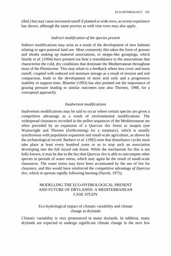
(ibid.) but may cause increased runoff if planted in wide rows, as recent experiencehas shown, although the same proviso as with vine rows may also apply.
Indirect modification of the species present
Indirect modifications may arise as a result of the development of new habitatsrelating to agro-pastoral land use. Most commonly this takes the form of grassesand shrubs making up matorral associations, or steppe-like groupings, whichSturdy et al. (1994) have pointed out bear a resemblance to the associations thatcharacterise the cold, dry conditions that dominate the Mediterranean throughoutmost of the Pleistocene. This may relate to a feedback where less cover and morerunoff, coupled with reduced soil moisture storage as a result of erosion and soilcompaction, leads to the development of more arid soils and a progressiveinability to support trees. Blumler (1993) has also pointed out the importance ofgrazing pressure leading to similar outcomes (see also Thornes, 1988, for aconceptual approach).
Inadvertent modifications
Inadvertent modifications may be said to occur where certain species are given acompetitive advantage as a result of environmental modifications. Thewidespread clearances recorded in the pollen sequences of the Mediterranean areoften preceded by an expansion of a Quercus ilex forest or maquis (seeWainwright and Thornes (forthcoming) for a summary), which is usuallysynchronous with population expansion and small-scale agriculture, as shown bythe archaeological record. Barbero et al. (1992) note that disturbance cycles musttake place at least every hundred years or so to stop such an associationdeveloping into the full mixed oak forest. While the mechanism for this is notfully known, it may be due to the fact that Quercus ilex is able to outcompete otherspecies in periods of water stress, which may again be the result of small-scaleclearances. The water stress may have been accentuated by the use of fire forclearance, and this would have reinforced the competitive advantage of Quercusilex, which re-sprouts rapidly following burning (Naveh, 1975).
MODELLING THE ECO-HYDROLOGICAL PRESENTAND FUTURE OF DRYLANDS: A MEDITERRANEAN
CASE STUDY
Eco-hydrological impact of climatic variability and climatechange in drylands
Climatic variability is very pronounced in many drylands. In addition, manydrylands are expected to undergo significant climate change in the next few
ECO-HYDROLOGY 101
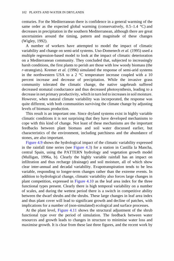
centuries. For the Mediterranean there is confidence in a general warming of thesame order as the expected global warming (conservatively, 0.5–1.4 °C) anddecreases in precipitation in the southern Mediterranean, although there are greatuncertainties around the timing, pattern and magnitude of these changes(Wigley, 1992).
A number of workers have attempted to model the impact of climaticvariability and change on semi-arid systems. Uso-Domenech et al. (1995) used amultiple regression-based model to look at the impact of climatic deteriorationon a Mediterranean community. They concluded that, subjected to increasinglyharsh conditions, the first plants to perish are those with low woody biomass (ther-strategists). Kremer et al. (1996) simulated the response of semi-arid systemsin the northwestern USA to a 2 °C temperature increase coupled with a 10percent increase and decrease of precipitation. While the invasive grasscommunity tolerated the climatic change, the native sagebrush suffereddecreased stomatal conductance and thus decreased photosynthesis, leading to adecrease in net primary productivity, which in turn led to increases in soil moisture.However, when natural climate variability was incorporated, the response wasquite different, with both communities surviving the climate change by adjustinglevels of biomass production.
This result is an important one. Since dryland systems exist in highly variableclimatic conditions it is not surprising that they have developed mechanisms tocope with this kind of change. Not least of these mechanisms are the importantfeedbacks between plant biomass and soil water discussed earlier, butcharacteristics of the environment, including patchiness and the abundance ofstones, are also important.
Figure 4.9 shows the hydrological impact of the climatic variability expressedin the rainfall time series (see Figure 4.3) for a station in Castilla la Mancha,central Spain, using the PATTERN hydrology and vegetation growth model(Mulligan, 1996a, b). Clearly the highly variable rainfall has an impact oninfiltration and thus recharge (drainage) and soil moisture, all of which showclear inter-annual and decadal variability. Evapotranspiration tends to be lessvariable, responding to longer-term changes rather than the extreme events. Inaddition to hydrological change, climatic variability also forces large changes inplant competition, expressed in Figure 4.10 as the leaf area index for the threefunctional types present. Clearly there is high temporal variability on a numberof scales, and during the wettest period there is a switch in competitive abilitybetween the dwarf shrubs and the shrubs. These large changes in leaf area indexand thus plant cover will lead to significant growth and decline of patches, withimplications for a number of (non-simulated) ecological and surface processes.
At the plant level, Figure 4.11 shows the structural adjustment of the shrubfunctional type over the period of simulation. The feedback between waterresources and growth leads to changes in structure to minimise water loss andmaximise growth. It is clear from these last three figures, and the recent work by
102 PLANTS AND WATER IN DRYLANDS
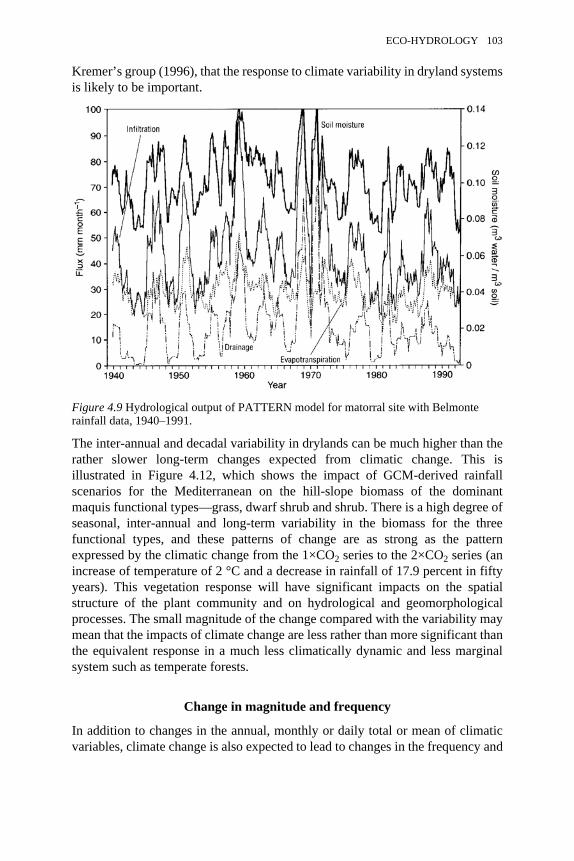
Kremer’s group (1996), that the response to climate variability in dryland systemsis likely to be important.
Figure 4.9 Hydrological output of PATTERN model for matorral site with Belmonterainfall data, 1940–1991.
The inter-annual and decadal variability in drylands can be much higher than therather slower long-term changes expected from climatic change. This isillustrated in Figure 4.12, which shows the impact of GCM-derived rainfallscenarios for the Mediterranean on the hill-slope biomass of the dominantmaquis functional types—grass, dwarf shrub and shrub. There is a high degree ofseasonal, inter-annual and long-term variability in the biomass for the threefunctional types, and these patterns of change are as strong as the patternexpressed by the climatic change from the 1×CO2 series to the 2×CO2 series (anincrease of temperature of 2 °C and a decrease in rainfall of 17.9 percent in fiftyyears). This vegetation response will have significant impacts on the spatialstructure of the plant community and on hydrological and geomorphologicalprocesses. The small magnitude of the change compared with the variability maymean that the impacts of climate change are less rather than more significant thanthe equivalent response in a much less climatically dynamic and less marginalsystem such as temperate forests.
Change in magnitude and frequency
In addition to changes in the annual, monthly or daily total or mean of climaticvariables, climate change is also expected to lead to changes in the frequency and
ECO-HYDROLOGY 103
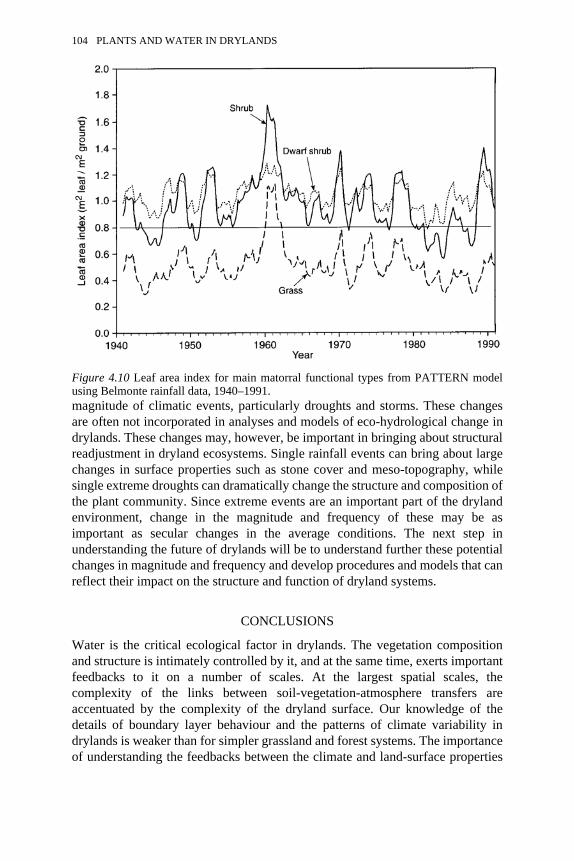
magnitude of climatic events, particularly droughts and storms. These changesare often not incorporated in analyses and models of eco-hydrological change indrylands. These changes may, however, be important in bringing about structuralreadjustment in dryland ecosystems. Single rainfall events can bring about largechanges in surface properties such as stone cover and meso-topography, whilesingle extreme droughts can dramatically change the structure and composition ofthe plant community. Since extreme events are an important part of the drylandenvironment, change in the magnitude and frequency of these may be asimportant as secular changes in the average conditions. The next step inunderstanding the future of drylands will be to understand further these potentialchanges in magnitude and frequency and develop procedures and models that canreflect their impact on the structure and function of dryland systems.
CONCLUSIONS
Water is the critical ecological factor in drylands. The vegetation compositionand structure is intimately controlled by it, and at the same time, exerts importantfeedbacks to it on a number of scales. At the largest spatial scales, thecomplexity of the links between soil-vegetation-atmosphere transfers areaccentuated by the complexity of the dryland surface. Our knowledge of thedetails of boundary layer behaviour and the patterns of climate variability indrylands is weaker than for simpler grassland and forest systems. The importanceof understanding the feedbacks between the climate and land-surface properties
Figure 4.10 Leaf area index for main matorral functional types from PATTERN modelusing Belmonte rainfall data, 1940–1991.
104 PLANTS AND WATER IN DRYLANDS
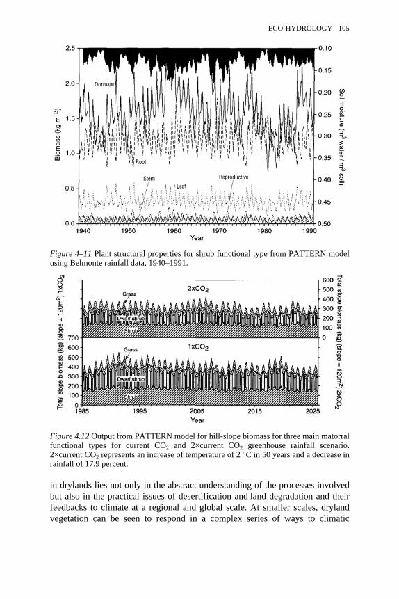
in drylands lies not only in the abstract understanding of the processes involvedbut also in the practical issues of desertification and land degradation and theirfeedbacks to climate at a regional and global scale. At smaller scales, drylandvegetation can be seen to respond in a complex series of ways to climatic
Figure 4–11 Plant structural properties for shrub functional type from PATTERN modelusing Belmonte rainfall data, 1940–1991.
Figure 4.12 Output from PATTERN model for hill-slope biomass for three main matorralfunctional types for current CO2 and 2×current CO2 greenhouse rainfall scenario.2×current CO2 represents an increase of temperature of 2 °C in 50 years and a decrease inrainfall of 17.9 percent.
ECO-HYDROLOGY 105

variability on all timescales. Perhaps the most important processes in this caseare the ways in which plants and communities respond to minimise the impact ofsuch variability. A number of mechanisms have been identified, such as delayedresponses and growth cycles and the development of clumped or bandedstructures. At a regional scale, the general models for runoff production andsediment transport in drylands developed over the last forty years seem to beapplicable. However, at smaller scales, there are many details of theinterrelationships between vegetation clumps, runoff production and erosion ofsediments and nutrients that are only beginning to be understood.
Modelling can be seen as a useful way of developing our understanding of eco-hydrological processes in drylands, where data acquisition is often particularlydifficult. Models with high spatial resolution and temporal resolutions that cancope with both rapidly occurring and longer-term processes are necessary. ThePATTERN model developed by Mulligan (1996a, b) is used here to presentsome example results to illustrate how such models can be used to predict futurechanges in dryland environments.
On longer timescales, it can be seen that Mediterranean vegetation groupingsare a relatively recent development. Although their origins can be seen in thelater Pliocene, the types of association we see at the present time do not reallystabilise until the last 600 ka. In this sense, they are a much later grouping thanassociations seen for example in Africa or North America. Over at least the last6000 years, human activity can be seen to be possibly the most important controlon Mediterranean eco-hydrology.
ACKNOWLEDGEMENTS
JW would like to acknowledge the role of Tony Parsons and Athol Abrahams indeveloping ideas and carrying out the work on overland flow and erosion in theAmerican southwest. The field experiments described from Walnut Gulch wereundertaken with the assistance and cooperation of the USDA-ARS SouthwestWatershed Research Center, Tucson. Ken Renard, Gary Frasier, David Woolhiser,Leonard Lane and Mark Weltz are thanked for permission to use the facilities atthe Tombstone field station, as are Roger Simanton and the technicians atTombstone for their generous advice and assistance. The experiments describedat Jornada were undertaken as part of the Jornada Long-Term EcologicalResearch project supported by the National Science foundation (Grant DEB 94–11971). None of the above-named, of course, is responsible for any errors andomissions contained herein.
MM would like to acknowledge UK NERC for the studentship GT4/91/AAPS/4 under which most of the modelling work was developed. The modelling wascarried out with data support from the EFEDA I and II projects and the SpanishNational Meteorological Office.
Rainfall data mentioned in this chapter have been supplied courtesy of Météo-France, the Spanish National Meteorological Office, Kris Havstad of USDA-
106 PLANTS AND WATER IN DRYLANDS
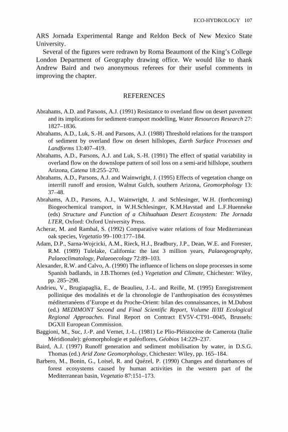
ARS Jornada Experimental Range and Reldon Beck of New Mexico StateUniversity.
Several of the figures were redrawn by Roma Beaumont of the King’s CollegeLondon Department of Geography drawing office. We would like to thankAndrew Baird and two anonymous referees for their useful comments inimproving the chapter.
REFERENCES
Abrahams, A.D. and Parsons, A.J. (1991) Resistance to overland flow on desert pavementand its implications for sediment-transport modelling, Water Resources Research 27:1827–1836.
Abrahams, A.D., Luk, S.-H. and Parsons, A.J. (1988) Threshold relations for the transportof sediment by overland flow on desert hillslopes, Earth Surface Processes andLandforms 13:407–419.
Abrahams, A.D., Parsons, A.J. and Luk, S.-H. (1991) The effect of spatial variability inoverland flow on the downslope pattern of soil loss on a semi-arid hillslope, southernArizona, Catena 18:255–270.
Abrahams, A.D., Parsons, A.J. and Wainwright, J. (1995) Effects of vegetation change oninterrill runoff and erosion, Walnut Gulch, southern Arizona, Geomorphology 13:37–48.
Abrahams, A.D., Parsons, A.J., Wainwright, J. and Schlesinger, W.H. (forthcoming)Biogeochemical transport, in W.H.Schlesinger, K.M.Havstad and L.F.Huenneke(eds) Structure and Function of a Chihuahuan Desert Ecosystem: The JornadaLTER, Oxford: Oxford University Press.
Acherar, M. and Rambal, S. (1992) Comparative water relations of four Mediterraneanoak species, Vegetatio 99–100:177–184.
Adam, D.P., Sarna-Wojcicki, A.M., Rieck, H.J., Bradbury, J.P., Dean, W.E. and Forester,R.M. (1989) Tulelake, California: the last 3 million years, Palaeogeography,Palaeoclimatology, Palaeoecology 72:89–103.
Alexander, R.W. and Calvo, A. (1990) The influence of lichens on slope processes in someSpanish badlands, in J.B.Thornes (ed.) Vegetation and Climate, Chichester: Wiley,pp. 285–298.
Andrieu, V., Brugiapaglia, E., de Beaulieu, J.-L. and Reille, M. (1995) Enregistrementpollinique des modalités et de la chronologie de l’anthropisation des écosystèmesméditerranéens d’Europe et du Proche-Orient: bilan des connaissances, in M.Dubost(ed.) MEDIMONT Second and Final Scientific Report, Volume II/III EcologicalRegional Approaches. Final Report on Contract EV5V-CT91–0045, Brussels:DGXII European Commission.
Baggioni, M., Suc, J.-P. and Vernet, J.-L. (1981) Le Plio-Pléistocène de Camerota (ItalieMéridionale): géomorphologie et paléoflores, Géobios 14:229–237.
Baird, A.J. (1997) Runoff generation and sediment mobilisation by water, in D.S.G.Thomas (ed.) Arid Zone Geomorphology, Chichester: Wiley, pp. 165–184.
Barbero, M., Bonin, G., Loisel, R. and Quézel, P. (1990) Changes and disturbances offorest ecosystems caused by human activities in the western part of theMediterranean basin, Vegetatio 87:151–173.
ECO-HYDROLOGY 107
Barbero, M., Loisel, R. and Quézel, P. (1992) Biogeography, ecology and history ofMediterranean Quercus ilex ecosystems, Vegetatio 99–100:19–34.
Beatley, J.C. (1974) Phenological events and their environmental triggers in MojaveDesert ecosystems, Ecology 55:856–863.
Beatley, J.C. (1976) Vascular plants of the Nevada test site and central-southern Nevada:ecology and geographical distribution, National Technical Information ServiceTID-26881, Springfield, Va.: US Department of Commerce, 306 pp.
Bertoldi, R., Rio, D. and Thunell, R. (1989) Pliocene—Pleistocene vegetational andclimatic evolution of the south-central Mediterranean, Palaeogeography,Palaeoclimatology, Palaeoecology 72:263–275.
Betts, A., Sellers, P.J. and Hall, F.G. (1992) FIFE in 1992—results, scientific gains, andfuture research directions, Journal of Geophysical Research—Atmospheres 97, D17:19091–19109.
Blumler, M.A. (1993) Successional pattern and landscape sensitivity in Mediterraneanand Near East, in D.S.G.Thomas and R.J.Allison (eds) Landscape Sensitivity,Chichester: Wiley, pp. 287–308.
Blyth, E.M., Dolman A.J. and Noilhan, J. (1994) The effect of forest on mesoscale rainfall—an example from HAPEX-MOBILHY, Journal of Applied Meteorology 33(4):445–454.
Bolle, H.-J., Andre, J.C., Arrue, J.L., Barth, H.K., Bessemoulin, P., Brasa, A., de Bruin,H.A.R., Cruces, J., Dugdale, G., Engman, E.T., Evans, D.L., Fantechi, R., Fiedler,F., van de Griend, A., Imeson, A.C., Jochum, A., Kabat, P., Hratzsch, T., Lagouarde,J.-P., Langer, I., Llamas, R., Lopez-Baeza, E., Melia Miralles, J., Muniosguren, L.S.,Nerry, F., Noilhan, J., Oliver, H.R., Roth, R., Saatchi, S.S., Sanchez Diaz, J., deSanta Olalla, M., Shuttleworth, W.J., Sogaard, H., Stricker, H., Thornes, J.B.,Vauclin, M. and Wickland, D. (1993) European field experiment in desertificationthreatened areas, Annales Geophysicae 11:173–189.
Brandt, C.J. (1986) Transformation of the kinetic energy of rainfall with variable treecanopies, unpublished PhD thesis, University of London. Brandt, C.J. (1989) Thesize distribution of throughfall drops under vegetation canopies, Catena 16:507–524.
Braud, I., Dantas-Antonino, A.C. and Vauclin, M. (1995) A stochastic approach tostudying the influence of the spatial variability of soil hydraulic properties on surfacefluxes, temperature and humidity, Journal of Hydrology 165(1–4): 283–310.
Carraro, F. (ed.) with contributions from 35 others (1996) Revisione del Villafranchianonell’area-tipo di Villafranca d’Asti, Il Quaternario 9(1):5–120.
Cerdà, A. (1997) The effect of patchy distribution of Stipa tenacissima L. on runoff anderosion, Journal of Arid Environments 36:37–51.
Childs, S.W. and Flint, A.L. (eds) (1990) Physical Properties of Forest Soils ContainingRock Fragments, 7th North American Forest Soils Conference, Vancouver: ForestryPublications, University of British Columbia.
Christensen, N.L. (1994) The effects of fire on physical and chemical properties of soils inMediterranean-climate shrublands, in J.M.Moreno and W.C.Oechel (eds) The Roleof Fire in Mediterranean-Type Ecosystems, New York: Springer-Verlag, pp. 79–95.
Clemens, S.C. and Tiedemann, R. (1997) Eccentricity forcing of Pliocene-EarlyPleistocene climate revealed in a marine oxygen-isotope record, Nature 385:801–804.
COHMAP members (1988) Climatic changes of the last 18,000 years; observations andmodel predictions, Science 241:1043–1052.
108 PLANTS AND WATER IN DRYLANDS
Combourieu-Nebout, N. (1993) Vegetation response to Upper Pliocene glacial/interglacial cyclicity in the central Mediterranean, Quaternary Research 40:228–236.
Daget, P. (1980) Un élément actuel de la caractérisation du monde Méditerranéen: leclimat, in Colloque de la Fondation L. Emberger sur ‘la mise en place, l’évolution etla caractérisation de la flore et de la végétation circumméditerranéennes’,Montpellier 9–10 April 1980. Naturalia Monspeliensia, No. Hors Série, pp. 101–126.
Dale, V.H. (1997) The relationship between land use change and climatic change,Ecological Applications 7(3):753–769.
Davis, F.W. and Burrows, D.A. (1994) Spatial simulation of fire regime in Mediterranean-climate landscapes, in J.M.Moreno and W.C.Oechel (eds) The Role of Fire inMediterranean-Type Ecosystems, New York: Springer-Verlag, pp. 117–139.
de Lima, M.I.L.P. and de Lima, J.L.M.P. (1990) Water erosion of soils containing rockfragments, in U.Shamir and C.J.Aqi (eds) The Hydrological Basis for WaterManagement (Proceedings of the Beijing Symposium, October 1990), Wallingford:IASH Publication No. 197, pp. 141–147.
Dirmeyer, P.A. and Shukla, J. (1994) Albedo as a modulator of climate response totropical deforestation, Journal of Geophysical Research—Atmospheres 99, D10:20863–20877.
Douglas, I. (1967) Man, vegetation and the sediment yield of rivers, Nature 215:925–928.
Dunkerley, D.L. (1997) Banded vegetation: survival under drought and grazing pressurebased on a simple cellular automaton model, Journal of Arid Environments 35(3):419–428.
Eltahir, E.A.B. and Bras, R.L. (1994) Sensitivity of regional climate to deforestation inthe Amazon Basin , Advances in Water Resources 17(1–2):101–115.
Elwell, H.A. and Stocking, M.A. (1976) Vegetal cover to estimate soil erosion hazard inRhodesia, Geoderma 15:61–70.
Evenari, M. (1985a) The desert environment, in M.Evenari, I.Noy-Meir and D.W.Goodall
(eds) Hot Deserts and Arid Shrublands. Ecosystems of the World 12A, Amsterdam:Elsevier, 1–19.
Evenari, M. (1985b) Adaptations of plants and animals to the desert environment, inM.Evenari, I.Noy-Meir and D.W.Goodall (eds) Hot Deserts and Arid Shrublands.Ecosystems of the World 12A, Amsterdam: Elsevier, 79–92.
Follieri, M., Magri, D. and Sadori, L. (1988) 250,000-year pollen record from Valle diCastiglione (Roma), Pollen et Spores XXX: 329–356.
Gasse, F., Fontes, J.C., Plaziat, J.C., Carbonel, P., Kaczmarska, I., De Deckker, P., Soulie-Marsche, I., Callot, Y. and Dupeuble, P.A. (1987) Biological remains, geochemistryand stable isotopes for the reconstruction of environmental and hydrological changesin the Holocene lakes from north Sahara. Palaeogeography, Palaeoclimatology,Palaeoecology 60:1–46.
Goutorbe, J.P., Lebel, T., Tinga, A., Bessemoulin, P., Brouwer, J., Dolman, A.J.,Engman, E.T., Gash, J.H.C., Hoepffner, M., Kabat, P., Kerr, Y.H., Monteny, B.,Prince, S., Said, F., Sellers, P. and Wallace, J.S. (1994) HAPEX-Sahel— a large-scale study of land-atmosphere interactions in the semi-arid Tropics, AnnalesGeophysicae—Atmospheres, Hydrospheres and Space Sciences 12(1): 53–64.
Graf, W.L. (1988) Fluvial Processes in Dryland Rivers, Berlin: Springer Verlag.
ECO-HYDROLOGY 109
Grove, A.T. (1957) Patterned ground in northern Nigeria, Geographical Journal 124:528–533.
Guiot, J. (1987) Late Quaternary climate change in France estimated from multivariatepollen time series, Quaternary Research 28:100–118.
Hall, F.G. and Sellers, P.J. (1995) First international satellite land-surface climatologyproject (ISLSCP) field experiment (FIFE) in 1995, Journal of Geophysical Research— Atmospheres 100, D12:25383–25395.
Henderson-Sellers, A. (1994) Land use change and climate, Land Degradation andRehabilitation 5(2):107–126.
Horowitz, A. (1989) Continuous pollen diagrams for the last 3.5 m.y. from Israel:vegetation, climate and correlation with the oxygen isotope record,Palaeogeography, Palaeoclimatology, Palaeoecology 72:63–78.
Horowitz, A. and Horowitz, M. (1985) Subsurface late Cenozoic palynostratigraphy ofthe Hula Basin, Israel, Pollen et Spores XXVII(3–4):365–390. Imeson, A.C.,Verstraten, J.M., van Mulligen, E.J. and Sevink, J. (1992) The effects of fire andwater repellency on infiltration and runoff under Mediterranean type forest, Catena19:345–361.
Inbar, M. (1992) Rates of fluvial erosion in basins with a Mediterranean type climate,Catena 19:393–409.
Jeltsch, F., Milton, S.J., Dean, W.R.J. and van Rooyen, N. (1996) Tree spacing andcoexistence in semi-arid savannas, Journal of Ecology 84:583–595.
Keigwin, L.D. and Thunell, R.C. (1979) Middle Pliocene climatic change in the westernMediterranean from faunal and oxygen isotope trends, Nature 282: 292–296.
Kirkby, M.J. (1990) A simulation model for desert runoff and erosion, inErosion, Transport and Deposition Processes, Proceedings of the JerusalemWorkshop, Wallingford: IAHS Publication No. 189, pp. 87–104.
Kirkby, M.J. and Neale, R.H. (1987) A soil-erosion model incorporating seasonal factors,in V.G.Gardiner (ed.) International Geomorphology, Proceedings of the FirstInternational Conference of Geomorphology, Manchester, UK, Chichester: Wiley,189–210.
Kirkby, M.J., Baird, A.J., Diamond, S.M., Lockwood, J.G., McMahon, M.L., Mitchell,P.L., Shao, J., Sheehy, J.E., Thornes, J.B. and Woodward, F.I. (1996) TheMEDALUS slope catena model: a physically based process model for hydrology,ecology and land degradation interactions, in C.J.Brandt and J.B.Thornes (eds)Mediterranean Desertification and Land Use, Chichester: Wiley, pp. 303–354.
Kosmas, C., Danalatos, N., Cammeraat, L.H., Chabart, M., Diamantopoulos, J., Farrand,R., Gutiérrez, M., Jacob, A., Marques, H., Martinez-Fernandez, J., Mizara, A.,Moustakas, N., Nicolau, J.M., Oliveros, C., Pinna, G., Puddu, R., Puigdefábregas, J.,Roxo, M., Simao, A., Stamou, G., Tomasi, N., Usai, D. and Vacca, A. (1997) Theeffect of landuse on runoff and soil erosion rates under Mediterranean conditions,Catena 29:45–59.
Koster, R.D. and Suarez, M.J. (1994) The components of a SVAT scheme and theireffects on a GCM’s hydrological cycle, Advances in Water Resources 17(1–2):61–78.
Kremer, R.G., Hunt, E.R., Running, S.W. and Coughlan, J.C. (1996) Simulatingvegetational and hydrologic responses to natural climatic variation and GCM-predicted climate change in a semi-arid ecosystem in Washington, USA, Journal ofArid Environments 33:23–38.
110 PLANTS AND WATER IN DRYLANDS
Kutiel, P. and Inbar, M. (1993) Fire impacts on soil nutrients and soil erosion in aMediterranean pine forest plantation, Catena 20:129–139.
Langbein, W.B. and Schumm, S.A. (1958) Yield of sediment in relation to mean annualprecipitation, Transactions of the American Geophysical Union 39: 1076–1084.
Laval, H., Medus, J. and Roux, M. (1991) Palynological and sedimentological records ofHolocene human impact from the Étang de Berre, southeastern France, TheHolocene 1:269–272.
Le Houérou, H.N. (1986) The desert and arid zones of northern Africa, in M.Evenari,I.Noy-Meir and D.W.Goodall (eds) Ecosystems of the World 12B, Hot Deserts andArid Shrublands B. Amsterdam: Elsevier, pp. 101–147.
Le Houérou, H.N. (1997) Climate, flora and fauna changes in the Sahara over the past 500million years, Journal of Arid Environments 37:619–647.
Lean, J.J. and Rowntree, P.R. (1997) Understanding the sensitivity of a GCM simulationof Amazonian deforestation to the specification of vegetation and soilcharacteristics, Journal of Climate 10(6):1216–1235.
Lefever R. and Lejeune, O. (1997) On the origin of tiger bush, Bulletin of MathematicalBiology 59(2):263–294.
Levin, N. and Horowitz, A. (1987) Palynostratigraphy of the Early Pleistocene QIpalynozone in the Jordan-Dead Sea Rift, Israel’, Israel Journal of Earth Sciences 36:45–58.
Mabbutt, J.A. and Fanning, P.C. (1987) Vegetation banding in arid Western Australia,Journal of Arid Environments 12:41–59.
MacFadyen, W.A. (1950) Vegetation patterns in the semi-desert plains of BritishSomaliland, Geographical Journal 116:199–211.
Maley, J. (1990) Les changements climatiques de la fin du Tertiaire en Afrique: leurconséquence sur l’apparition du Sahara et de sa végétation, in M.A.J.Williams andH.Faure (eds) The Sahara and the Nile. Quaternary Environments and PrehistoricOccupation in Northern Africa, Rotterdam: A.A.Balkema, pp. 63–86.
Marengo, J.A., Miller, J.R., Russell, G.L., Rosenzweig, C.E. and Abramopoulos, F.(1994) Calculations of river runoff in the GISS GCM—impact of a new land-surfaceparameterization and runoff routing model on the hydrology of the Amazon River,Climate Dynamics 10(6–7):349–361.
Martinez-Mesa, E. and Whitford, W.G. (1996) Stemflow, throughfall and channel-izationof stemflow by roots in three Chihuahuan desert shrubs, Journal of AridEnvironments 32:271–287.
Meehl, G.A. and Washington, W.M. (1988) A comparison of soil moisture sensitivity intwo global climate models, Journal of Atmospheric Science 45: 1476–1492.
Mommersteeg, H.J.P.M., Loutre, M.F., Young, R., Wijmstra, T.A. and Hooghiemstra, H.(1995) Orbital forced frequencies in the 975,000 year pollen record from TenaghiPhilippon (Greece), Climate Dynamics 11:4–24.
Monteith, J.L. (1973) Principles of Environmental Physics, London: Edward Arnold.Morgan, R.P.C. (1996) Verification of the European soil erosion model (EUROSEM) for
varying slope and vegetation conditions, in M.G.Anderson and S.M.Brooks (eds)Advances in Hillslope Processes, Chichester: Wiley, pp. 657–668.
Mulligan, M. (1996a) Modelling hydrology and vegetation change in a degraded semi-arid environment, unpublished PhD thesis, King’s College, University of London.
ECO-HYDROLOGY 111
Mulligan, M. (1996b) Modelling the complexity of land surface response to climaticvariability in Mediterranean environments , in M.G.Anderson and S.M.Brooks (eds)Advances in Hillslope Processes, Chichester: Wiley, pp. 1099–1149.
Naveh, Z. (1967) Mediterranean ecosystems and vegetation types in California and Israel,Ecology 48:445–459.
Naveh, Z. (1975) The evolutionary significance of fire in the Mediterranean region,Vegetatio 29:199–209.
Noilhan J., Lacarrere, P., Dolman, A.J. and Blyth, E.M. (1997) Defining area-averageparameters in meteorological models for land surfaces with mesoscale heterogeneity,Journal of Hydrology 190(3–4):302–316.
Nulsen, R.A., Bligh, K.J., Baxter, I.N., Solin, E.J. and Imrie, D.H. (1986) The fate ofrainfall in a malle and heath vegetated catchment in southern Western Australia,Australian Journal of Ecology 11:361–371.
O’Brien, K.L. (1996) Tropical deforestation and climate change, Progress in PhysicalGeography 20(3):311–335. Obando, J.A. (1996) Modelling the impact of landabandonment on runoff and soil erosion in a semi-arid catchment, unpublished PhDthesis, King’s College, University of London.
Parsons, A.J., Abrahams, A.D. and Luk, S.-H. (1991) Size characteristics of sediment ininterrill overland flow on a semi-arid hillslope, southern Arizona, Earth SurfaceProcesses and Landforms 16:143–152.
Parsons, A.J., Abrahams, A.D. and Simanton, J.R. (1992) Microtopography and soil-surface materials on semi-arid piedmont hillslopes, Journal of Arid Environments22:107–115.
Parsons, A.J., Abrahams, A.D. and Wainwright, J. (1994) Rainsplash and erosion rates inan interrill area on semi-arid grassland, southern Arizona, Catena 22: 215–226.
Parsons, A.J., Wainwright, J. and Abrahams, A.D. (1993) Tracing sediment movement ininterrill overland flow on a semi-arid grassland hillslope using magneticsusceptibility, Earth Surface Processes and Landforms 18:721–732.
Parsons, A.J., Wainwright, J. and Abrahams, A.D. (1996a) Runoff and erosion on semi-arid hillslopes, in M.G.Anderson and S.M.Brooks (eds) Advances in HillslopeProcesses, Chichester: Wiley, pp. 1061–1078.
Parsons, A.J., Abrahams, A.D. and Wainwright, J. (1996b) Responses of interrill runoffand erosion rates to vegetation change in southern Arizona, Geomorphology 14:311–317.
Parsons, A.J., Wainwright, J., Abrahams, A.D. and Simanton, J.R. (1997) Distributeddynamic modelling of interrill overland flow, Hydrological Processes 11:1833–1859.
Pearson, G.W. and Stuiver, M. (1993) High-precision bidecadal calibration of theradiocarbon time scale, 500–2500 BC, Radiocarbon 35:25–33.
Pelgrum, H. and Bastiaanssen, W.G.M. (1996) An intercomparison of techniques todetermine the area-averaged latent-heat flux from individual in-situ observa-tions—aremote-sensing approach using the European field experiment in a desertification-threatened area data, Water Resources Research 32(9):2775–2786.
Poesen, J. (1986) Surface sealing as influenced by slope angle and position of simulatedstones in the top layer of loose sediments, Earth Surface Processes and Landforms11:1–10.
112 PLANTS AND WATER IN DRYLANDS
Poesen, J. and Bunte, K. (1995) Effects of rock fragments on desertification processes inMediterranean environments, in J.B.Thornes and C.J.Brandt (eds) MediterraneanDesertification and Land Use, Chichester: Wiley, pp. 247–269.
Poesen, J., Ingelmo-Sanchez, F. and Mucher, H. (1990) The hydrological response of soilsurfaces to rainfall as affected by cover and position of rock fragments in the toplayer, Earth Surface Processes and Landforms 15:653–671.
Polcher, J. and Laval, K. (1994) A statistical study of the regional impact of deforestationon climate in the LMD GCM, Climate Dynamics 10(4–5):205–219.
Pons, A. and Reille, M. (1988) The Holocene and Upper Pleistocene pollen record fromPadul (Granada, Spain): a new study, Palaeogeography, Palaeoclimatology,Palaeoecology 66:243–263.
Pons, A., Guiot, J., de Beaulieu, J.-L. and Reille, M. (1992) Recent contributions to theclimatology of the last glacial-interglacial cycle based on French pollen sequences,Quaternary Science Reviews 11:439–448.
Pope, K.O. and van Andel, T.H. (1984) Late Quaternary alluviation and soil formation inthe southern Argolid: its history, causes and archaeological implications, Journal ofArchaeological Science 11:281–306.
Pressland, A.J. (1973) Rainfall partitioning by an arid woodland (Acacia aneura F.Meull.)in south-western Queensland, Australian Journal of Botany 21: 235–245.
Puigdefábrigas, J. and Sánchez, G. (1996) Geomorphological implications of vegetationpatchiness on semi-arid slopes, in M.G.Anderson and S.M.Brooks (eds) Advances inHillslope Processes, Chichester: Wiley, pp. 1027–1060.
Quézel, P. (1978) Analysis of the flora of Mediterranean and Saharan Africa, AnnalsMissouri Botanical Garden 65:479–534.
Reynolds, J.F., Virginia, R.A., Kemp, P.R., de Soyza, A.G. and Tremmel, D.C., (in press)Impact of simulated drought on resource islands of shrubs in the Chihuahuan Desert:effects of species, season, and degree of island development, Ecology.
Ritchie, J.C., Eyles, C.H. and Haynes, C.V. (1985) (sic) Sediment and pollen evidence foran early to mid-Holocene humid period in the eastern Sahara. Nature 314:352–355.
Rogers, R.D. and Schumm, S.A. (1991) The effect of sparse vegetative cover on erosionand sediment yield, Journal of Hydrology 123:19–24.
Rosa Attolini, M., Galli, M., Nanni, T., Ruggiero, L. and Zuanni, F. (1988) Preliminaryobservations of the fossil forest of Dunarobba (Italy) as a potential archive ofpaleoclimatic information, Dendrochronologia 6:33–48.
Rostagno, C.M. and del Valle, H.F. (1988) Mounds associated with shrubs in aridic soilsof northeastern Patagonia: characteristics and probable genesis, Catena 15: 347–359.
Rumney, G.R. (1968) Climatology and the World’s Climates. New York: Macmillan.Sánchez, G. and Puigdefábregas, J. (1994) Interactions of plant growth and sediment
movement on slopes in a semi-arid environment, Geomorphology 9:243–260.Savat, J. and Poesen, J. (1981) Detachment and transportation of loose sediment by
raindrop splash. Part I: The calculation of absolute data on detachability andtransportability, Catena 8:1–17.
Schlesinger, W.H., Abrahams, A.D., Parsons, A.J. and Wainwright, J. (in press) Nutrientlosses in runoff from grassland and shrubland habitats in southern New Mexico: I.Rainfall simulation experiments, Biogeochemistry.
Schlesinger, W.H., Reynolds, J.F., Cunningham, G.L., Huenneke, L.F., Jarrell, W.M.,Virginia, R.A. and Whitford, W.G. (1990) Biological feedbacks in globaldesertification, Science 247:1043–1048.
ECO-HYDROLOGY 113
Schumm, S.A. (1965) Quaternary palaeohydrology, in H.E.Wright and D.G.Frey (eds)The Quaternary of the United States, Princeton, NJ: Princeton University Press,pp. 783–794.
Scoging, H.M. (1982) Spatial variations in infiltration, runoff and erosion on hillslopes insemi-arid Spain, in R.B.Bryan and A.Yair (eds) Badland Geomorphology and Piping,Norwich: GeoBooks, pp. 89–112.
Scoging, H.M. and Thornes, J.B. (1979) Infiltration characteristics in a semi-aridenvironment, in Proceedings of the Canberra Symposium on the Hydrology of Areasof Low Precipitation, Wallingford: IASH Publication No. 128, 159–168.
Sene, K.J. (1996) Meteorological estimates for the water balance of a sparse vine cropgrowing in semiarid conditions, Journal of Hydrology 179(1–4):259–280.
Shackleton, N.J. and Opdyke, N.D. (1977) Oxygen isotope and palaeomagnetic evidencefor early Northern Hemisphere glaciation , Nature 270:216–219.
Shmida, A. (1972) The vegetation of Gebel Maghara, North Sanai, unpublished PhDthesis, The Hebrew University, Jerusalem.
Shmida, A. (1985) Biogeography of the desert flora, in M.Evenari, I.Noy-Meir, andD.W.Goodall (eds) Hot Deserts and Arid Shrublands. Ecosystems of the World 12A,pp. 23–72, Amsterdam: Elsevier.
Shukla, J. and Mintz, Y. (1982) The influence of land-surface evapo-transpiration on theEarth’s climate, Science 215:1498–1501.
Shuttleworth, W.M. and Wallace, J.S. (1985) Evaporation from sparse crops—an energycombination theory, Quarterly Journal of the Royal Meteorological Society 111:839–856.
Shuttleworth, W.J, Gash, J.H.C., Roberts, J.M., Nobre, C.A., Molion, L.C.B. and Ribeiro,M.D.G. (1991) Post-deforestation Amazonian climate—Anglo-Brazilian research toimprove prediction, Journal of Hydrology 129(1–4):71–85.
Smith, E.A., Wai, M.M.K., Cooper, H.J. and Rubes, M.T. (1994) Linking boundary-layercirculations and surface processes during FIFE-89. 1. Observational analysis,Journal of the Atmospheric Sciences 51(11):1497–1529.
Soler, M. and Sala, M. (1992) Effects of fire and of clearing in a Mediterranean Quercusilex woodland: an experimental approach, Catena 19:321–332.
Specht, R.L. (1972) Water use by perennial evergreen plant communities in Australia andPapua New Guinea, Australian Journal of Botany 20:273–299.
Starkel, L. (1983) The reflection of hydrologic changes in the fluvial environment of thetemperate zone during the last 15,000 years, in K.J.Gregory (ed.) Background toPalaeohydrology, Chichester: Wiley, pp. 213–235.
Starkel, L. (1987) The evolution of European rivers—a complex response, in K.J.Gregory, J.Lewin and J.B.Thornes (eds) Palaeohydrology in Practice, Chichester:Wiley, pp. 333–339.
Stockdale, T., Latif, M., Burgers, G. and Wolff, J.O. (1994) Some sensitivities of acoupled ocean-atmosphere GCM, Tellus Series A—Dynamic Meteorology andOceanography 46(4):367–380.
Stuiver, M. and Pearson, G.W. (1993) High-precision bidecadal calibration of theradiocarbon time scale, AD 1950–500 BC and 2500–6000 BC, Radiocarbon 35:1–23.
Stuiver, M. and Reimer, P.J. (1993) Extended C14 data-base and revised Calib 3.0 C14 agecalibration program, Radiocarbon 35:215–230.
Sturdy, D., Webley, D. and Bailey, G.N. (1994) Prehistoric land use, in S.E.van der
114 PLANTS AND WATER IN DRYLANDS
Leeuw (ed.) Understanding the Natural and Anthropogenic Causes of Soil Degradationand Desertification in the Mediterranean Basin. Volume 1: Land Degradation inEpirus, Final Report on Contract EV5V-CT91–0021, Brussels: DGXII EuropeanCommission, pp. 81–142.
Suc, J.-P. (1984) Origin and evolution of the Mediterranean vegetation and climate inEurope, Nature 307:429–432.
Suc, J.-P. and Bessais, E. (1990) Pérennité d’un climat thermo-xériquie en Sicile avant,pendant, après la crise de salinité messinienne, Comptes Rendus de l’Académie desSciences de Paris, Série II 310:1701–1707.
Suc, J.-P. and Zagwijn, W.H. (1983) Plio-Pleistocene correlations between thenorthwestern Mediterranean region and northwestern Europe according to recentbiostratigraphic and palaeoclimatic data, Boreas 12:153–166.
Sud, Y.C., Shukla, J. and Mintz, Y. (1985) Influence of Land Surface Roughness onAtmospheric Circulation and Rainfall: A Sensitivity Experiment with a GCM. NASATechnical Memo 86219, 233 pp.
Sud, Y.C., Walker, G.K., Kim, J.-H., Listen, G.E., Sellers, P.J. and Lau, K.M. (1996)Biogeophysical consequences of a tropical deforestation scenario: a GCM
simulation study, Journal of Geophysical Research 101, D3:7095–7109.Terradas, J. and Savé, R. (1992) The influence of summer and winter stress and water
relationships on the distribution of Quercus ilex L., Vegetatio 99–100:137–145.Tilman, D. (1994) Competition and biodiversity in spatially structured habitats, Ecology,
75:2–16.Thornes, J.B. (1988) Erosional equilibria under grazing, in J.Bintliff, D.Davidson and
E.Grant (eds) Conceptual Issues in Environmental Archaeology. Edinburgh:Edinburgh University Press, 193–210.
Thornes, J.B. (1990) The interaction of erosional and vegetational dynamics in landdegradation: spatial outcomes, in J.B.Thornes (ed.) Vegetation and Erosion,Chichester: Wiley, 41–53.
Thunell, R.C. (1979) Climatic evolution of the Mediterranean Sea during the last 5.0million years, Sedimentary Geology 23:67–79.
Thunell, R.C. and Williams, D.F. (1983) Paleotemperature and paleosalinity history of theeastern Mediterranean during the late Quaternary, Palaeogeography,Palaeoclimatology, Palaeoecology 44:23–39.
Torri, D., Sfalanga, M. and del Sette, M. (1981) Splash detachment: runoff depth and soilcohesion, Catena 14:149–155.
Turner, J. and Greig, J.R.A. (1975) Some Holocene pollen diagrams from Greece, Reviewof Palaeobotany and Palynology 20:171–204.
Tzedakis, P.C. (1994) Vegetation change through glacial-interglacial cycles: a long-termpollen-sequence perspective, Philosophical Transactions of the Royal Society ofLondon 345B:403–432.
UNEP (1977) Desertification: its Causes and Consequences, Nairobi: First United NationsConference on Desertification.
UNEP (1991) Status of Desertification and Implementation of the United Nations Plan ofAction to Combat Desertification, Nairobi: UNEP.
UNEP/ISRIC (1992) World Atlas of Desertification, London: Edward Arnold.Uso-Domenech, J.L., Villacampa-Esteve, Y., Stubing-Martinez, G., Karjalainen, T. and
Ramo, M.P. (1995) MARIOLA: a model for calculating the response of
ECO-HYDROLOGY 115
Mediterranean bush ecosystem to climatic variations, Ecological Modelling 80:113–129.
Valentine, I. and Nagorcka, B.N. (1979) Contour patterning in Atriplex vesicariacommunities, in D.Graetz and K.M.W.Howes (eds) Studies of the Australian AridZone. Part 4, Melbourne: CSIRO, pp. 121–146.
van Andel, T.H. and Runnels, C. (1987) Beyond the Acropolis. A Rural Greek Past,Stanford, Calif: Stanford University Press,
van Andel, T., Runnels, C.N. and Pope, K.O. (1986) Five thousand years of land use andabuse in the southern Argolid, Greece, Hesperia 55:103–128.
van Andel, T.H., Zangger, E. and Demitrack, A. (1990) Land use and soil erosion inprehistoric and historical Greece, Journal of Field Archaeology 17:379–396.
van der Maarel, E. (1988) Vegetation dynamics: patterns of change in time and space,Vegetalio 77:7–19.
van der Wiel, A.M. and Wijmstra, T.A. (1987a) Palynology of the lower part (78–120 m)of the core Tenaghi Philippon II, Middle Pleistocene of Macedonia, Greece, Reviewof Palaeobotany and Palynology 52:73–88.
van der Wiel, A.M. and Wijmstra, T.A. (1987b) Palynology of the 112.8–197.8 m intervalof the core Tenaghi Philippon III, Middle Pleistocene of Macedonia, Review ofPalaeobotany and Palynology 52:89–117.
van Zinderen Bakker, E.M. (1983) Elements for the chronology of Late Cainozoic Africanclimates, in W.C.Mahaney (ed.) Correlation of Quaternary Chronologies, Norwich:GeoBooks, pp. 23–38.
Vega, J.A. and Diaz Fiernos, F. (1987) Wildfire effects on soil erosion, EcologiaMediterranea XIII:119–125.
Vergnaud-Grazzini, C., Saliège, J.F., Urrutiager, M.J. and Iannace, A. (1990) Oxygen andcarbon isotope stratigraphy of ODP Hole 653A and site 654: the Pliocene-Pleistocene glacial history recorded in the Tyrrhenian Basin (West Mediterranean),in K.A.Kastens, J.Mascle et al. (eds) Proceedings of the Ocean Drilling Program.Volume 107 Scientific Results. Tyrrhenian Sea, College Station TX: Ocean DrillingProgram, pp. 361–386.
Vernet, J.-L. and Thiébault, S. (1987) An approach to northwestern Mediterranean recentprehistoric vegetation and ecologic implications, Journal ofBiogeography 14:117–127.
Wainwright, J. (1992) Assessing the impact of erosion on semi-arid archaeological sites,in M.Bell and J.Boardman (eds) Past and Present Soil Erosion, Oxford: OxbowBooks, pp. 228–41.
Wainwright, J. (1996a) Climats actuels et passes: implications humaines, in J. Gascó,L.Carozza, S.Fry, R.Fry, J.-D.Vigne and J.Wainwright (eds) Le Laouret et laMontagne d’Alaric à la Fin de l’Âge du Bronze, un hameau abandonné entre Floureet Monze (Aude), Toulouse: Centre d’Anthropologie, pp. 45–56.
Wainwright, J. (1996b) Infiltration, runoff and erosion characteristics of agricultural landin extreme storm events, SE France, Catena 26:27–47.
Wainwright, J. (1996c) A comparison of the infiltration, runoff and erosion characteristicsof two contrasting ‘badland’ areas in S.France, Zeitschrift für GeomorphologieSupplementband 106:183–198.
Wainwright, J. (1997) History and Evolution of Mediterranean Desertification, King’sCollege London: Concerted Action on Mediterranean Desertification ThematicReport.
116 PLANTS AND WATER IN DRYLANDS
Wainwright, J. (in press, a) Climate and climatological variation, in W.H. Schlesinger,K.M.Havstad and L.F.Huenneke (eds) Structure and Function of a ChihuahuanDesert Ecosystem: The Jornada LTER. Oxford: Oxford University Press.
Wainwright, J. (in press, b) Contextes géomorphologiques et géoarchéologiques deshabitats de l’Âge du Bronze en Méditerranée Occidentale, in Proceedings, XXIVeCongrès Préhistorique de France.
Wainwright, J. and Thornes, J.B. (forthcoming) Environmental Issues in theMediterranean, Routledge: London.
Wainwright, J., Parsons, A.J. and Abrahams, A.D. (1995) Simulation of raindrop erosionand the development of desert pavements, Earth Surface Processes and Landforms20:277–291.
Wainwright, J., Parsons, A.J. and Abrahams, A.D. (in press) Field and computersimulation experiments on the formation of desert pavement, Earth SurfaceProcesses and Landforms.
Walker, J. and Rowntree, P.R. (1987) The effect of soil moisture on circulation andrainfall in a tropical model, Quarterly journal of the Royal Meteorological Society103: 29–46.
Wallace, J.S. and Holwill, C.J. (1997) Soil evaporation from tiger-bush in southwestNiger, Journal of Hydrology 189(1–4):426–442.
Walling, D.E. and Webb, B.W. (1983) Patterns of sediment yield, in K.J.Gregory (ed.)Background to Palaeohydrology, Chichester: Wiley, pp. 69–100.
Warren, A. and Khogali, M. (1992) Assessment of Desertification and Drought in theSudano-Sahelian Region 1985–1991, New York: United Nations Sudano-SahelianOffice.
Watts, W.A., Allen, J.R.M. and Huntley, B. (1996) Vegetation history and palaeoclimateof the last glacial period at Lago Grande di Monticchio, southern Italy, QuaternaryScience Reviews 15:133–153.
Whitford, W.G. (1997) Desertification and animal biodiversity in the desert grasslands ofNorth America, Journal of Arid Environments 37:709–720.
Wigley, T.M.L. (1992) Future climate of the Mediterranean Basin with particularemphasis on changes in precipitation, in L.Jeftic, J.D.Milliman and G.Sestini (eds)Climatic Change and the Mediterranean: Environmental and Societal Impacts ofClimatic Change and Sea-Level Rise in the Mediterranean Region, London: EdwardArnold, pp. 15–44.
Wijmstra, T.A. (1969) Palynology of the first 30 metres of a 120 m deep section innorthern Greece, Acta Botanica Neerlandica 18:511–527.
Wijmstra, T.A. and Smit, A. (1976) Palynology of the middle part (30–78 metres) of the120 m deep section in northern Greece (Macedonia), Acta Botanica Neerlandica 25:297–312.
Willis, K.J. (1994) The vegetational history of the Balkans, Quaternary Science Reviews13:769–788.
Wilson, M.F., Henderson-Sellers, A., Dickinson, R.E. and Kennedy, P.J. (1987)Investigation of the sensitivity of the land surface parameterisation of the NCARcommunity climate model in regions of tundra vegetation, Journal of Climatology 7:319–343.
Wood, E.F. (1997) Effects of soil moisture aggregation on surface evaporative fluxes,Journal of Hydrology 190(3–4):397–412.
ECO-HYDROLOGY 117

Woodward, F.I. (1994) Vegetation growth modelling, in J.B.Thornes (ed.) Third InterimReport for Medalus II, pp. 61–65, EV5V-CT92–0128, Brussels: DGXII EuropeanCommission.
Worral, G.A. (I960) Patchiness in vegetation in the northern Sudan, Journal of Ecology48:107–115.
Wright, H.E., Kutzbach, J.E., Webb III, T., Ruddiman, W.F., Street-Perrott, F.A. andBartlein, P.J. (eds) (1993) Global Climates Since the Last Glacial Maximum,Minneapolis: University of Minnesota Press.
Xue, Y.K. and Shukla, J. (1996) The influence of land surface properties on Sahel climate.Part II: afforestation, Journal of Climate 9(12):3360–3275.
Zhang, X., Drake, N.A., Wainwright, J. and Mulligan, M. (1997) Global scale overlandflow and soil erosion modelling using remote sensing and GIS techniques: modelimplementation and scaling, in Proceedings of RSS ’97 Remote Sensing in Action, 2–4 September, Reading, Nottingham: Remote Sensing Society, pp. 379–384.
118 PLANTS AND WATER IN DRYLANDS

5WATER AND PLANTS IN FRESHWATER
WETLANDSBryan D.Wheeler
INTRODUCTION
The most characteristic feature of wetlands is that they are wet. The effects ofexcess water dominate their formation and considerably control their processesand characteristics. The fundamental importance of water availability to thecharacter of all wetlands, and the fact that certain types of wetland (peatlands)are largely based upon the remains of plants preserved by waterlogging, meanthat any consideration of ‘wetland plants and water’ could easily become areview of much of wetland ecology. However, this review will be more selectiveand focus particularly upon (1) mechanisms of adaptation of wetland plants towaterlogged environments; (2) quantitative effects of water availability andregimes upon the distribution of wetland plants and upon the composition ofwetland vegetation; (3) some effects of wetland plants upon the hydrologicalcharacteristics of the wetlands in which they grow; and (4) outline effects ofwater quality (chemical composition) upon the distribution of wetland plants.Consideration is restricted to freshwater wetlands.
The concept of ‘wetland’
The term ‘wetland’ is used widely, but not consistently. It has been variouslyapplied to a range of watery habitats, with differences of definition relatingmainly to the position of the upper and lower limits (Mitsch and Gosselink,1986). The Ramsar Convention on Wetlands of International Importance (1971)adopted a particularly broad concept, including habitats that are only periodicallywet and with low summer water tables (e.g. wet meadows, pond margins) andthose that are permanently inundated with up to 6 m of water. It is not difficult tofind reasons why aquatic and wet terrestrial systems should be grouped togetherunder a generic title of ‘wetlands’ (not least their frequent hydraulic andontogenic links), but it is equally clear that many ecological processes operatedifferently in the two types. From many (though not all) viewpoints, ‘wet land’ ismore usefully seen as a particularly wet terrestrial ecosystem than an especially
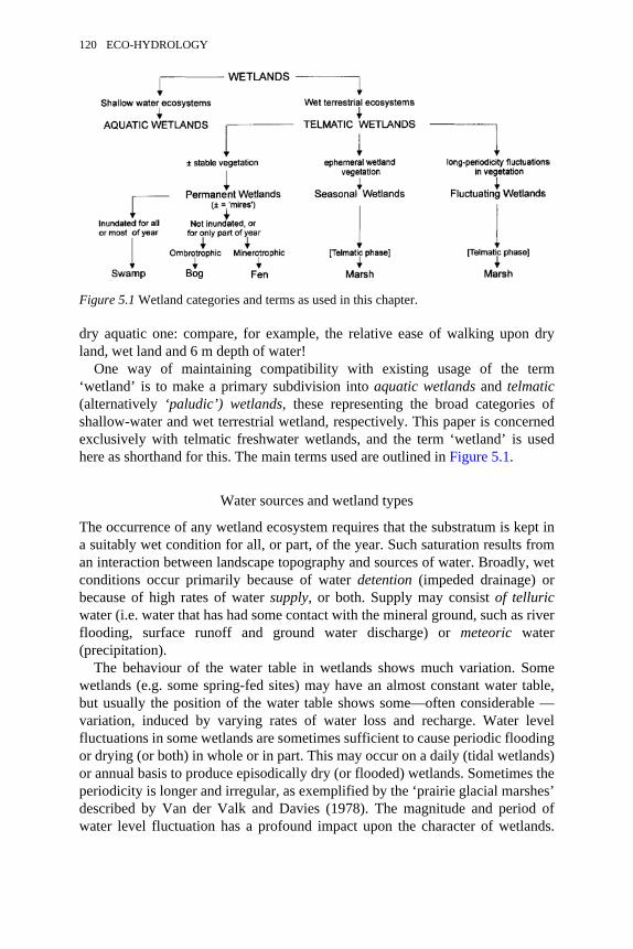
dry aquatic one: compare, for example, the relative ease of walking upon dryland, wet land and 6 m depth of water!
One way of maintaining compatibility with existing usage of the term‘wetland’ is to make a primary subdivision into aquatic wetlands and telmatic(alternatively ‘paludic’) wetlands, these representing the broad categories ofshallow-water and wet terrestrial wetland, respectively. This paper is concernedexclusively with telmatic freshwater wetlands, and the term ‘wetland’ is usedhere as shorthand for this. The main terms used are outlined in Figure 5.1.
Water sources and wetland types
The occurrence of any wetland ecosystem requires that the substratum is kept ina suitably wet condition for all, or part, of the year. Such saturation results froman interaction between landscape topography and sources of water. Broadly, wetconditions occur primarily because of water detention (impeded drainage) orbecause of high rates of water supply, or both. Supply may consist of telluricwater (i.e. water that has had some contact with the mineral ground, such as riverflooding, surface runoff and ground water discharge) or meteoric water(precipitation).
The behaviour of the water table in wetlands shows much variation. Somewetlands (e.g. some spring-fed sites) may have an almost constant water table,but usually the position of the water table shows some—often considerable —variation, induced by varying rates of water loss and recharge. Water levelfluctuations in some wetlands are sometimes sufficient to cause periodic floodingor drying (or both) in whole or in part. This may occur on a daily (tidal wetlands)or annual basis to produce episodically dry (or flooded) wetlands. Sometimes theperiodicity is longer and irregular, as exemplified by the ‘prairie glacial marshes’described by Van der Valk and Davies (1978). The magnitude and period ofwater level fluctuation has a profound impact upon the character of wetlands.
Figure 5.1 Wetland categories and terms as used in this chapter.
120 ECO-HYDROLOGY
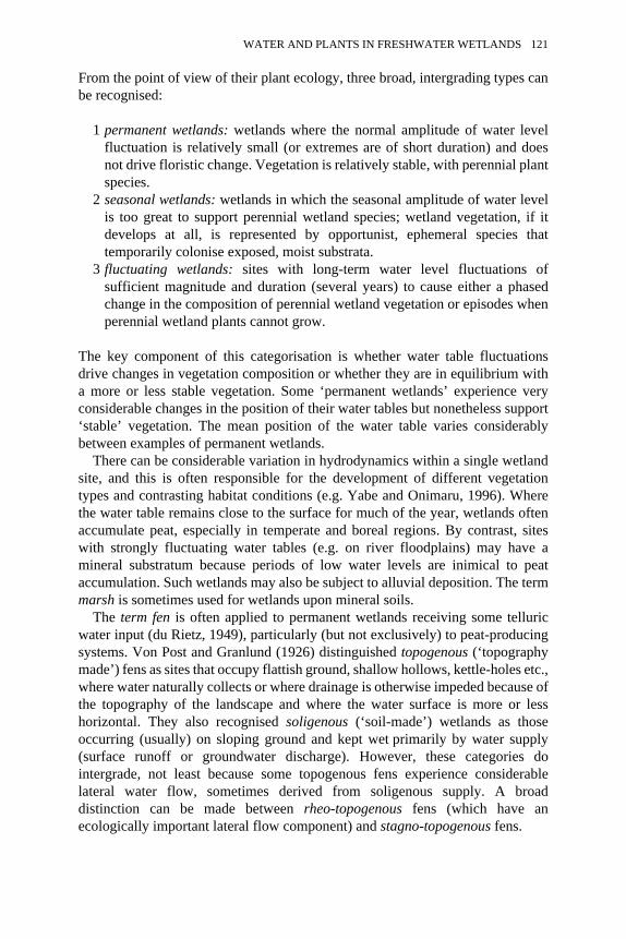
From the point of view of their plant ecology, three broad, intergrading types canbe recognised:
1 permanent wetlands: wetlands where the normal amplitude of water levelfluctuation is relatively small (or extremes are of short duration) and doesnot drive floristic change. Vegetation is relatively stable, with perennial plantspecies.
2 seasonal wetlands: wetlands in which the seasonal amplitude of water levelis too great to support perennial wetland species; wetland vegetation, if itdevelops at all, is represented by opportunist, ephemeral species thattemporarily colonise exposed, moist substrata.
3 fluctuating wetlands: sites with long-term water level fluctuations ofsufficient magnitude and duration (several years) to cause either a phasedchange in the composition of perennial wetland vegetation or episodes whenperennial wetland plants cannot grow.
The key component of this categorisation is whether water table fluctuationsdrive changes in vegetation composition or whether they are in equilibrium witha more or less stable vegetation. Some ‘permanent wetlands’ experience veryconsiderable changes in the position of their water tables but nonetheless support‘stable’ vegetation. The mean position of the water table varies considerablybetween examples of permanent wetlands.
There can be considerable variation in hydrodynamics within a single wetlandsite, and this is often responsible for the development of different vegetationtypes and contrasting habitat conditions (e.g. Yabe and Onimaru, 1996). Wherethe water table remains close to the surface for much of the year, wetlands oftenaccumulate peat, especially in temperate and boreal regions. By contrast, siteswith strongly fluctuating water tables (e.g. on river floodplains) may have amineral substratum because periods of low water levels are inimical to peataccumulation. Such wetlands may also be subject to alluvial deposition. The termmarsh is sometimes used for wetlands upon mineral soils.
The term fen is often applied to permanent wetlands receiving some telluricwater input (du Rietz, 1949), particularly (but not exclusively) to peat-producingsystems. Von Post and Granlund (1926) distinguished topogenous (‘topographymade’) fens as sites that occupy flattish ground, shallow hollows, kettle-holes etc.,where water naturally collects or where drainage is otherwise impeded because ofthe topography of the landscape and where the water surface is more or lesshorizontal. They also recognised soligenous (‘soil-made’) wetlands as thoseoccurring (usually) on sloping ground and kept wet primarily by water supply(surface runoff or groundwater discharge). However, these categories dointergrade, not least because some topogenous fens experience considerablelateral water flow, sometimes derived from soligenous supply. A broaddistinction can be made between rheo-topogenous fens (which have anecologically important lateral flow component) and stagno-topogenous fens.
WATER AND PLANTS IN FRESHWATER WETLANDS 121
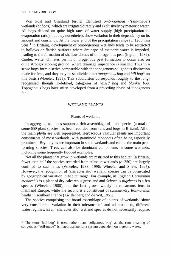
Von Post and Granlund further identified ombrogenous (‘rain-made’)wetlands (or bogs), which are irrigated directly and exclusively by meteoric water.All bogs depend on quite high rates of water supply (high precipitation-to-evaporation ratio), but they nonetheless show variation in their dependency on itsamount and constancy. At the lower end of the precipitation range (c. 1200 mmyear−1 in Britain), development of ombrogenous wetlands tends to be restrictedto hollows or flattish surfaces where drainage of meteoric water is impeded,leading to the formation of shallow domes of ombrogenous peat (Ingram, 1982).Cooler, wetter climates permit ombrogenous peat formation to occur also onquite strongly sloping ground, where drainage impedance is smaller. Thus in asense bogs form a series comparable with the topogenous-soligenous distinctionmade for fens, and they may be subdivided into topogenous bog and hill bog* onthis basis (Wheeler, 1995). This subdivision corresponds roughly to the long-recognised, though ill-defined, categories of raised bog and blanket bog.Topogenous bogs have often developed from a preceding phase of topogenousfen.
WETLAND PLANTS
Plants of wetlands
In aggregate, wetlands support a rich assemblage of plant species (a total ofsome 650 plant species has been recorded from fens and bogs in Britain). All ofthe main phyla are well represented. Herbaceous vascular plants are importantconstituents of most wetlands, with graminoid monocots often being especiallyprominent. Bryophytes are important in some wetlands and can be the main peat-forming species. Trees can also be dominant components in some wetlands,including some frequently flooded examples.
Not all the plants that grow in wetlands are restricted to this habitat. In Britain,fewer than half the species recorded from telmatic wetlands (c. 250) are largelyconfined to such sites (Wheeler, 1988; 1996; Wheeler and Shaw, 1995).However, the recognition of ‘characteristic’ wetland species can be obfuscatedby geographical variation in habitat range. For example, in England Herminiummonorchis is a plant of dry calcareous grassland and Schoenus nigricans is a fenspecies (Wheeler, 1988), but the first grows widely in calcareous fens inmainland Europe, while the second is a constituent of summer-dry Rosmarinusheaths in southern France (Zwillenberg and de Wit, 1951).
The species comprising the broad assemblage of ‘plants of wetlands’ showvery considerable variation in their tolerance of, and adaptation to, differentwater regimes. Even ‘characteristic’ wetland species do not necessarily require,
* The term ‘hill bog’ is used rather than ‘soligenous bog’ as the root meaning ofsoligenous (‘soil-made’) is inappropriate for a system dependent on meteoric water.
122 ECO-HYDROLOGY
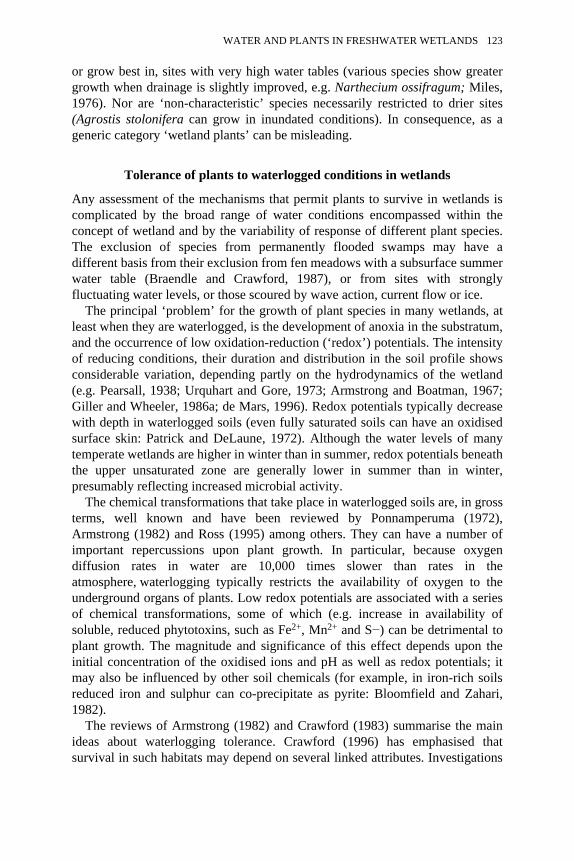
or grow best in, sites with very high water tables (various species show greatergrowth when drainage is slightly improved, e.g. Narthecium ossifragum; Miles,1976). Nor are ‘non-characteristic’ species necessarily restricted to drier sites(Agrostis stolonifera can grow in inundated conditions). In consequence, as ageneric category ‘wetland plants’ can be misleading.
Tolerance of plants to waterlogged conditions in wetlands
Any assessment of the mechanisms that permit plants to survive in wetlands iscomplicated by the broad range of water conditions encompassed within theconcept of wetland and by the variability of response of different plant species.The exclusion of species from permanently flooded swamps may have adifferent basis from their exclusion from fen meadows with a subsurface summerwater table (Braendle and Crawford, 1987), or from sites with stronglyfluctuating water levels, or those scoured by wave action, current flow or ice.
The principal ‘problem’ for the growth of plant species in many wetlands, atleast when they are waterlogged, is the development of anoxia in the substratum,and the occurrence of low oxidation-reduction (‘redox’) potentials. The intensityof reducing conditions, their duration and distribution in the soil profile showsconsiderable variation, depending partly on the hydrodynamics of the wetland(e.g. Pearsall, 1938; Urquhart and Gore, 1973; Armstrong and Boatman, 1967;Giller and Wheeler, 1986a; de Mars, 1996). Redox potentials typically decreasewith depth in waterlogged soils (even fully saturated soils can have an oxidisedsurface skin: Patrick and DeLaune, 1972). Although the water levels of manytemperate wetlands are higher in winter than in summer, redox potentials beneaththe upper unsaturated zone are generally lower in summer than in winter,presumably reflecting increased microbial activity.
The chemical transformations that take place in waterlogged soils are, in grossterms, well known and have been reviewed by Ponnamperuma (1972),Armstrong (1982) and Ross (1995) among others. They can have a number ofimportant repercussions upon plant growth. In particular, because oxygendiffusion rates in water are 10,000 times slower than rates in theatmosphere, waterlogging typically restricts the availability of oxygen to theunderground organs of plants. Low redox potentials are associated with a seriesof chemical transformations, some of which (e.g. increase in availability ofsoluble, reduced phytotoxins, such as Fe2+, Mn2+ and S−) can be detrimental toplant growth. The magnitude and significance of this effect depends upon theinitial concentration of the oxidised ions and pH as well as redox potentials; itmay also be influenced by other soil chemicals (for example, in iron-rich soilsreduced iron and sulphur can co-precipitate as pyrite: Bloomfield and Zahari,1982).
The reviews of Armstrong (1982) and Crawford (1983) summarise the mainideas about waterlogging tolerance. Crawford (1996) has emphasised thatsurvival in such habitats may depend on several linked attributes. Investigations
WATER AND PLANTS IN FRESHWATER WETLANDS 123
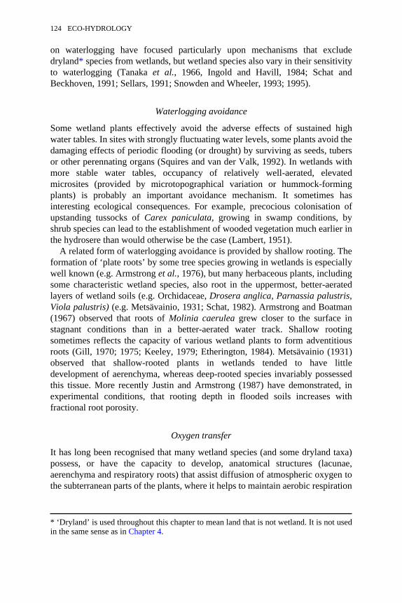
on waterlogging have focused particularly upon mechanisms that excludedryland* species from wetlands, but wetland species also vary in their sensitivityto waterlogging (Tanaka et al., 1966, Ingold and Havill, 1984; Schat andBeckhoven, 1991; Sellars, 1991; Snowden and Wheeler, 1993; 1995).
Waterlogging avoidance
Some wetland plants effectively avoid the adverse effects of sustained highwater tables. In sites with strongly fluctuating water levels, some plants avoid thedamaging effects of periodic flooding (or drought) by surviving as seeds, tubersor other perennating organs (Squires and van der Valk, 1992). In wetlands withmore stable water tables, occupancy of relatively well-aerated, elevatedmicrosites (provided by microtopographical variation or hummock-formingplants) is probably an important avoidance mechanism. It sometimes hasinteresting ecological consequences. For example, precocious colonisation ofupstanding tussocks of Carex paniculata, growing in swamp conditions, byshrub species can lead to the establishment of wooded vegetation much earlier inthe hydrosere than would otherwise be the case (Lambert, 1951).
A related form of waterlogging avoidance is provided by shallow rooting. Theformation of ‘plate roots’ by some tree species growing in wetlands is especiallywell known (e.g. Armstrong et al., 1976), but many herbaceous plants, includingsome characteristic wetland species, also root in the uppermost, better-aeratedlayers of wetland soils (e.g. Orchidaceae, Drosera anglica, Parnassia palustris,Viola palustris) (e.g. Metsävainio, 1931; Schat, 1982). Armstrong and Boatman(1967) observed that roots of Molinia caerulea grew closer to the surface instagnant conditions than in a better-aerated water track. Shallow rootingsometimes reflects the capacity of various wetland plants to form adventitiousroots (Gill, 1970; 1975; Keeley, 1979; Etherington, 1984). Metsävainio (1931)observed that shallow-rooted plants in wetlands tended to have littledevelopment of aerenchyma, whereas deep-rooted species invariably possessedthis tissue. More recently Justin and Armstrong (1987) have demonstrated, inexperimental conditions, that rooting depth in flooded soils increases withfractional root porosity.
Oxygen transfer
It has long been recognised that many wetland species (and some dryland taxa)possess, or have the capacity to develop, anatomical structures (lacunae,aerenchyma and respiratory roots) that assist diffusion of atmospheric oxygen tothe subterranean parts of the plants, where it helps to maintain aerobic respiration
* ‘Dryland’ is used throughout this chapter to mean land that is not wetland. It is not usedin the same sense as in Chapter 4.
124 ECO-HYDROLOGY
(e.g. Warming, 1909; Armstrong, 1980; Crawford, 1983; Justin and Armstrong,1987). Wetland plants also often have some capacity to produce oxidisingconditions in the rhizosphere of actively growing roots (e.g. Armstrong, 1964).This phenomenon is known as radial oxygen loss (ROL) and can be induced bythe radial diffusion of oxygen through the cortex or by enzymatic oxidation onthe root surface (Armstrong, 1967). The establishment of oxidising conditions inthe rhizosphere is thought to provide a mechanism that reduces the uptake of thesoluble reduced toxins, by their oxidative precipitation around or within the roots(Bartlett, 1961; Jones and Etherington, 1970; Jones, 1972) although in somecircumstances, by steepening the concentration gradient of reduced toxins, thisprocess may increase their uptake (Tessenow and Baynes, 1978). Oxidisingconditions in the rhizosphere can also promote nitrification (Laan et al., 1989),and this may contribute to the vigorous growth of such species as Glyceriamaxima in some wetland soils (Engelaar et al., 1995).
There can be little doubt that oxygen transfer provides the key to the survivalof vascular plant species in waterlogged conditions. Indeed, one adaptation ofsome plants to periodic submergence is accelerated shoot growth, to extendabove the level of flood (Squires and van der Valk, 1992; Blom et al., 1994;Yabe and Onimaru, 1996). Doubts about the capacity of gas transfer to supplysufficient oxygen to plant roots in waterlogged soils (e.g. Crawford, 1983) havebeen largely answered by a better understanding of aeration mechanisms(Armstrong et al. 1992; W. Armstrong et al., 1996), although even well-ventilated plants may still experience hypoxia or anoxia when growing instrongly reducing substrata, or if connection with the atmosphere is severed. Rootporosity of wetland plants is also positively correlated with their tolerance to Fe2
+ (Snowden and Wheeler, 1993; 1995), and capacity for oxygen transport andROL seems to be critical to iron tolerance. ROL is unlikely, however, to be theonly mechanism by which wetland plants accommodate reduced toxins: in iron-rich environments, the Fe shoot content of some wetland species can be muchgreater than in low-iron examples (Wheeler et al., 1985), and uptake of largeamounts of iron sometimes occurs (e.g. Eriophorum angustifolium; Mansfield,1990). Likewise, certain species (e.g. Acorus calamus, Phragmites australis)have some capacity to detoxify sulphide by formation of thiols within the rhizomes(Weber and Brändle, 1996; Fürtig et al., 1996)—although exposure to highsulphide concentrations can still be injurious to Phragmites (J.Armstrong et al.,1996).
The dynamics of oxygen transfer from shoots to roots are strongly dependenton shoot architecture and are related to overall shoot porosity (Justin andArmstrong, 1987), but even shoots with much pore space can have specificblockages to oxygen transfer. Conway (1937) concluded that the small cellsforming the intercalary meristems at the base of the growing leaves of Cladiummariscus provided an effective barrier to gaseous diffusion and proposed thatpersistent dead leaves were critical to aeration of the subterranean parts of this
WATER AND PLANTS IN FRESHWATER WETLANDS 125
plant. Likewise, Armstrong et al. (1992) point to the importance of old or brokenculms of Phragmites for rhizome ventilation.
Anaerobic metabolism
Wetland plants, and some flood-tolerant dryland species, may display variousmetabolic adaptations to survival of anoxia, some of which may act bystimulating adventitious root formation, aerenchyma development or stemelongation (e.g. ethylene production: Osborne, 1984; van der Sman et al., 1991).Roots of some, perhaps many, wetland plants can endure periods of anoxia, butearly ideas that wetland plants may be preferentially able to accumulate low-toxicity metabolites of anaerobic respiration (e.g. malíc acid) (MacMannon andCrawford, 1971; Crawford, 1983) seem to have been discarded in favour of theircapacity to tolerate high concentrations of ethanol, or to vent toxic metabolites intotheir surroundings. There seems little doubt that anaerobic metabolism mayprovide tolerance to short periods of waterlogging, but it is less clear what part itplays in long-term survival. Capacity for sustained anaerobic respiration isrelated to the magnitude of carbohydrate reserves (Schlüter et al., 1966; Weberand Brändle, 1966). Acorus calamus has an unusually large capacity to endureanoxia and can tolerate this for about three months (Weber and Brändle, 1966).Various species may depend on anaerobic respiration for over-wintering inanoxic sediments and, particularly, for regenerating new leaves and shoots (e.g.Kausch et al., 1981; Crawford, 1996). However, the reported ability of detachedrhizomes of Typha latifolia to tolerate anoxia (Barclay and Crawford, 1982) doesnot seem to eliminate the dependency of this species on emergent dead shootsfor over-wintering (Murkin and Ward, 1980). On balance, it seems likely that asubstantial capacity for anaerobic metabolism may be restricted to a few wetlandspecies, and it may provide a mechanism to endure short unfavourable periodsrather than prolonged tolerance.
Seed survival and establishment in wetlands
In some wetlands, periodic drought or deep flooding can exceed the tolerances ofsome or all established wetland plants and lead to their death. With the return ofappropriate conditions, re-establishment of wetland plants depends uponpersistent propagules in the substratum or upon inward dispersal. Seasonalwetlands typically have a well-developed seed bank, often dominated by annualspecies (Haukos and Smith, 1993), which can survive many years of flooding(Salisbury, 1970). Sites with longer periods of flood or drought can have seedbanks with a wider range of plant types (van der Valk and Davis, 1978; Keddyand Reznicek, 1982; Poiani and Johnson, 1989).
While re-establishment from seed is clearly important in seasonal andfluctuating wetlands, or in other sites subject to periodic damage (wave or currentscour), its significance in ‘undisturbed’ wetlands, which are often dominated by
126 ECO-HYDROLOGY
long-lived phanaerophytes, is much less certain and is often assumed to be small.Long-term, persistent seed banks are only formed by relatively few perennialphanaerophytes—particularly, although not exclusively, species subject tofrequent disturbance (Keddy and Reznicek, 1982; Voesenek and Blom, 1992)—although more have transient or short-term persistent reserves (Poschlod, 1995;Maas and Schopp-Guth, 1995). In particular, the rarer dicots, or those not verytolerant of waterlogged conditions (e.g. Primula farinosa), often do not havepersistent seed banks (Maas, 1989), perhaps partly because their seeds havelimited capacity to survive in a wetland environment (e.g. Caltha palustris(Skoglund, 1990); Betula pubescens (Skoglund and Verwijst, 1989)).
Ephemeral species are critically dependent upon detecting suitablegermination conditions. Some annual mudflat species germinate best inshallowly submerged soils (e.g. Elatine spp.), but many species may require avirtual absence of standing water (Van der Valk and Davis, 1978). Widetemperature fluctuation can be indicative of an absence of deep water cover, orof gaps within the vegetation canopy, and is the most important cue to thegermination of both ephemeral species (Baskin et al., 1993; van der Valk andDavis, 1978) and many perennials (Thompson and Grime, 1983; Maas, 1989).
Tolerance of wetland plants to dry soils
In natural moisture gradients, the upper limit of the distribution of particularwetland species may be controlled by sensitivity to moisture stress, butsurprisingly little attention has been paid to the tolerance of wetland plants to dryconditions. Nonetheless some, perhaps many, wetland plants can grow well inconditions drier than those in which they normally occur (e.g. Keddy, 1989),sometimes with reduced vigour (e.g. Conway, 1938; Wheeler et al., 1985). Thismay help explain why it can be difficult to demonstrate clear relationshipsbetween experimental estimates of drought susceptibility and the fielddistribution of some wetland species (Schat and Beckhoven, 1991).
The absence of wetland species from drier habitats may have several causes:desiccation damage induced through water stress; constraints uponestablishment; and competitive interactions with dryland species, in some casesconditioned by a reduction of vigour of wetland species in drier situations.
Water stress in wetland plants
Some wetland plants experience leaf water deficits, even in waterlogged soils(Bradbury and Grace, 1983), due both to high rates of water loss from the shootsand to constraints on water acquisition. Various wetland phanaerophytes havehigher rates of ‘cuticular’ water loss from their leaves than do dryland plants(Hygen, 1953; Willis and Jefferies, 1963), and some insectivorous species haveparticularly limited control of transpirative water loss (Hygen, 1953), probablybecause water is readily lost from the leaf surface through the thin-walled
WATER AND PLANTS IN FRESHWATER WETLANDS 127
secretory glands and tentacles. Other species may have inefficient stomatalcontrol of transpiration. Conway (1940) reported that leaves of Cladiummariscus developed water deficits in hot, bright conditions, even when the plantswere growing in water, and attributed this to restricted vascularisation. Manywetland species have shallow and meagre root systems (Metsävainio, 1931),adapted to avoid anoxia in waterlogged soils, and are little able to ‘forage’ forwater in drier conditions. Such constraints may partly explain the occurrence ofxeromorphic traits in some wetland plants (Schimper, 1898; Yapp, 1912),although some workers have suggested alternative possibilities. For example,Small (1973) concluded that xeromorphy had little to do with drought stress inbog plants but might be an incidental feature associated with slow growth innutrient-deficient or cold-stressed environments. Jones and Etherington (1970)suggest that reduction of transpiration may help to reduce the uptake of solubletoxins from waterlogged soils.
Bryophytes are poikilohydric and have little ability to regulate water gain orloss but vary considerably in their capacity to acquire water and to withstandsustained desiccation. A number of species, including taxa that normally grow invery wet conditions, can survive some droughting (e.g. Scorpidium scorpioides(Kooijman, 1993); Sphagnum cuspidatum (Luken, 1985; Heikkilä and Löytönen,1987)), although they may take longer to recover than do dryland species (Leeand Stewart, 1971; Bewley et al., 1978).
Constraints on seedling establishment and species interactions
Seedlings tend to be more drought-sensitive than mature plants, and the absenceof some wetland plants from dry soils may relate more to constraints on seedlingestablishment than to the tolerances of older plants (Ernst and Van der Ham,1988). There is evidence that seedlings of some wetland plants establish lesswell in dry soils than do those of some dryland species (Evans and Etherington,1991), in some cases, perhaps, because of an inability to produce questing rootsthat forage for a diminishing water supply (Reader et al., 1993).
There is also some evidence that some wetland species are restricted to wethabitats because potential competitor dryland species cannot grow so well in wetsoils (Ellenberg, 1954; Keddy, 1988; Keddy et al. 1994).
WATER REGIMES AND PLANTS OF WETLANDS
Relationships between species, vegetation and water tables
The position of the water table in wetland soils undoubtedly exerts a majorinfluence upon the distribution and performance of plant species and thecomposition of vegetation. This is especially obvious where there is a strongzonation of vegetation along a water level gradient, such as around the margins of
128 ECO-HYDROLOGY
lakes, where there may be a transition from swamp into fen and wet grassland,with woody vegetation (if present at all) often being furthest upslope (Spence,1964). On a smaller scale, microtopographical variation is often associated withcontrasting species distributions, as exemplified in the patterned surfaces ofsome ombrogenous bogs (Ratcliffe and Walker, 1958; Ivanov, 1981; see below).
Changing water tables also demonstrate the importance of water levels towetland vegetation. Some wetlands oscillate naturally between ‘dry’ and ‘wet’states and show compositional changes in time as well as space (e.g. van derValk and Davis, 1978). Others are subject to long-term persistent changes,sometimes induced artificially (by drainage, etc.). Substantial, progressivechange in water tables usually leads to some form of vegetation response,whether it be by flooding (e.g. Kadlec, 1962; Harris and Marshall, 1963;Rumberg and Sawyer, 1965; Sjöberg and Danell, 1983) or drying (Grootjans andTen Klooster, 1980; van der Valk and Davis, 1980; Fojt and Harding, 1995;Grootjans et al., 1996). Observed responses of established plants to hydrologicalchange depend upon the species and the magnitude of change and may includetruncation of range, or complete disappearance, of species incapable of growingin the new conditions; persistence in sub-optimal conditions, often with reducedvigour; change in position of species along the gradient (if the topographypermits); and continued, or even enhanced, growth in the new water depth range(Sjöberg and Danell, 1983). In addition, a range of new species may alsocolonise the new hydrological environment.
Numerous studies have examined the relationship between the distribution ofwetland plant species (or plant communities) and water levels (e.g. Tüxen, 1954;Willis et al., 1959a, b; Spence, 1964; Balátová-Tulácková, 1968; Klötzli, 1969;Mörnsjö, 1969; Jeglum, 1971; Niemann, 1963; Grootjans and Ten Klooster,1980; Egloff and Naef, 1982; Succow, 1988; Mooney and O’Connell, 1990;Scholle and Schrautzer, 1993). However, while it is possible to identify broadtrends in water table-plant distributions in wetlands, the range of conditionsoccupied by particular species or communities can be wide and may beinconsistent between, or even within, sites. For example, the water level ranges ofspecies and communities in shoreline zonations can differ considerably betweenlakes (Spence, 1964). There is some evidence that groups of species may showclearer relationships to water table behaviour than do individual species (Wierdaet al., 1997), but equally, because plant ‘communities’ are abstract, sometimesarbitrary and variable units, the use of syntaxa in exploring plant-environmentinterrelationships may sometimes be part of the problem rather than a road to itssolution (van Wirdum, 1986). Willis et al. (1959a, b) were unable to demonstratea sharp distinction between some communities in a dune slack toposequencebased on their ‘flooding index’. Thus, while it would be extremely desirable toestablish robust hydrological limits for species and communities, this is oftenproblematic. For example, Grootjans (1980) identified some water table limitsfor certain communities but, recognising the uncertainties involved, counselledagainst concluding that ‘drainage within the indicated limits can be done without
WATER AND PLANTS IN FRESHWATER WETLANDS 129
changing the floristic composition of the communities’—which suggests that thelimits proposed have little practical value.
Difficulties in detecting clear relationships between water tables and speciesor community distributions in wetlands may stem from various causes, not leastthat other environmental (or biotic) variables may help to determine distributions,either independently of water tables or by modifying species’ responses to waterconditions. However, difficulties also arise because water regimes are oftencomplex and difficult to characterise and relate to species distribution.Consideration of how variables influence species distributions in wetlandsindependently of water tables and water quality is outside the scope of thisreview, but attention will be given to some of the problems of relating speciesand vegetation to water table behaviour and to some of the ways in which otherenvironmental and biotic variables can modify the interrelationships betweenplants and water conditions.
Relating wetland plants and vegetation to water tablebehaviour
There are several reasons why it may be difficult to relate species distributionsand vegetation composition to water table behaviour:
1 Most studies are based on correlative procedures that assume equilibriumbetween the species (or vegetation) and the measured water regimes.
2 The behaviour of the water table in wetlands is often complex; it can bedifficult to characterise and to identify hydrological variables salient to thedistribution of plants; moreover, ‘controlling variables’ may differ fordifferent species and hydrological situations.
3 In some circumstances, soil moisture content may be more meaningful toplant growth than the position of the water table.
4 Most studies have been concerned with established plants, whereas in somecircumstances distributions may be determined by conditions that affectrecruitment.
5 Other variables may modify plant-water table interrelationships.
These are considered further below.
Equilibrium conditions
The majority of field studies on plant-water table relationships in wetlands havebeen based upon some form of correlation (e.g. Nilsson and Keddy, 1988).Recently, some workers have used optimum species response curves (Huismanet al., 1993) to explore these relationships (Spieksma et al., 1995; Wierda et al.,1997). Such approaches require some form of stable equilibrium between waterregime and vegetation, but this is more often assumed than investigated.
130 ECO-HYDROLOGY
When considering equilibrium conditions, a broad distinction must be madebetween situations where water level flux is of sufficient magnitude or durationto drive changes in vegetation composition and those in which changing waterlevels occur within, and may be characteristic of, a more or less stable plantcommunity. The first of these conditions is exemplified by the periodic drawdowncycle, and associated vegetation change, described for some prairie glacialmarshes by van der Valk and Davis (1978). Here, any attempt to identifyvegetation-water regime interrelationships would need to be made for each phasewithin the cycle—overall measurement would be meaningless. However, evenwithin individual phases the vegetation is not necessarily in equilibrium with thebehaviour of the water table (van der Valk and Davis, 1980).
Even in more stable wetlands, assumption of equilibrium between water tablebehaviour and vegetation may be invalid, either because species distributionswithin a given water regime are in a state of change, or because inertia againstchange permits the persistence of some species in sub-optimal conditions(Grootjans, 1980; van Diggelen et al., 1991b; Spieksma et al., 1995). Ironically,many, perhaps most, hydrological studies are made within regions subject toconsiderable recent, and often ongoing, water management (drainage by waterengineers or re-wetting by conservation managers), where assumptions ofequilibrium may be questionable. Disequilibria are also likely to be evident insystems where major community boundaries (e.g. extent of woody vegetation)are determined more by occasional extreme events (e.g. periodic deep flooding)than by persistent ‘average’ conditions (Hill andKeddy, 1992).
Identification and characterisation of salient components ofwater table behaviour
At many sites, water tables show substantial, and sometimes erratic, variation,which may be difficult to characterise simply. Each location has an ‘average’water table (or ‘wetness’), around which fluctuations occur. These vary in theirmagnitude, duration, frequency and timing (seasonality). The importance ofthese components in relation to plant distribution (inundation versus deficit;duration versus magnitude; winter flooding versus summer flooding; averagevalues versus extremes; average extremes versus exceptional extremes) remainsto be established fully and varies between species and situations. For example,the critical variables in wetlands subjected to protracted periods of inundation arelikely to be different from those important in wetlands with high water tables butlimited flooding, or in sites that experience periods of low water levels.
Various studies have drawn attention to the importance of differentcomponents of water table behaviour in regulating species distributions andvegetation composition, but it is quite difficult to extract generalities from these.This is because there are a relatively small number of studies, and not all of thesehave considered every component of water table behaviour; some studies areconcerned with controls on species distribution or performance, others with
WATER AND PLANTS IN FRESHWATER WETLANDS 131
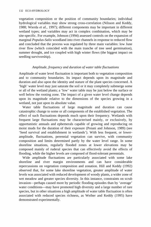
vegetation composition or the position of community boundaries; individualhydrological variables may show strong cross-correlation (Nilsson and Keddy,1988; Wierda et al., 1997); different components may be important in differentwetland types; and variables may act in complex combination, which may besite-specific. For example, Johnson (1994) assessed controls on the expansion ofmarginal Populus-Salix woodland into river channels in response to reduced flowand concluded that the process was regulated by three main variables: low Juneriver flow (which coincided with the main tranche of tree seed germination),summer drought, and ice coupled with high winter flows (the biggest impact onseedling survivorship).
Amplitude, frequency and duration of water table fluctuations
Amplitude of water level fluctuation is important both to vegetation compositionand to community boundaries. Its impact depends upon its magnitude andduration and also upon the identity and stature of the plant species concerned. A‘high’ water level may just saturate the soil or it may completely submerge someor all of the wetland plants; a ‘low’ water table may be just below the surface orwell below the rooting zone. The impact of a given water level change dependsupon its magnitude relative to the dimensions of the species growing in awetland, not just upon its absolute value.
Water table fluctuations of large magnitude and duration can causecatastrophic change to some or all components of the established vegetation. Theeffect of such fluctuations depends much upon their frequency. Wetlands withfrequent large fluctuations may be characterised mainly, or exclusively, byopportunistic annuals and ephemerals capable of growing and reproducing onmoist muds for the duration of their exposure (Poiani and Johnson, 1989) (see‘Seed survival and establishment in wetlands’). With less frequent, or lower-amplitude, fluctuations, perennial vegetation can survive, with communitycomposition and limits determined partly by the water level range. In someshoreline situations, regularly flooded zones at lower elevations may becomposed mainly of ruderal species that can effectively avoid the effects offlooding, while the higher levels are composed of flood-tolerant perennials.
Wide amplitude fluctuations are particularly associated with some lakeshoreline and river margin environments and can have considerablerepercussions on vegetation composition and zonation. Hill and Keddy (1992)observed that, for some lake shoreline vegetation, greater amplitude of waterlevels was associated with reduced development of woody plants, a wider zone ofwet meadow and greater species diversity. In this instance, constraints on scrubinvasion—perhaps caused more by periodic flooding episodes than by ‘average’water conditions—may have promoted high diversity and a large number of rarespecies, but in other situations a high amplitude of water table fluctuation is oftenassociated with reduced species richness, as Weiher and Keddy (1995) havedemonstrated experimentally.
132 ECO-HYDROLOGY
The duration of hydrological events is of much importance to the character ofwetland vegetation. In sites subjected to flooding episodes, species distributionscan be determined by the duration, as well as the depth, of inundation (Noest,1994). Tree species vary considerably in the duration of flooding that they cantolerate (Gill, 1970; Kozlowski, 1984), and, in wetlands subjected to regularwater level change, such as freshwater tidal wetlands, the lower limits of treespecies can be related to both the duration and frequency of periods of inundation(e.g. Zonneveld, 1959), although these effects are difficult to separate.
Long-period fluctuations can have particularly complex effects. Keddy andReznicek (1982) describe shoreline vegetation that varies from being species-poor in high-water phases to species-rich in low-water phases. They furthersuggest that the species richness of the low-water phase is itself partly a productof the unstable water environment, because the periodic high-water phasesprevent the establishment of dominance, and concomitant reduction of diversity,during the low-water phases.
In somewhat less variable hydrological contexts, Spieksma et al. (1995)suggest that the most discriminating variables (with regard to the occurrence ofplant communities) are the mean, highest and lowest groundwater levels togetherwith the possibility of inundation during the growing season. Wierda et al.(1997) concluded that mean highest water level was particularly important incontrolling the occurrence of plant species in some types of wetland, along withamplitude of fluctuation. Scholle and Schrautzer (1993) used the combination of‘average’ water level, a ‘groundwater fluctuation index’ (which assessed thefluctuation pattern) and the duration of inundation to characterise six waterregime types, each of which could be related quite closely to vegetationcomposition. Various workers have concluded that the cumulative period of timefor which a particular water level is exceeded can provide a sensitivecharacterisation of hydrological regimes with regard to vegetation composition(Willis et al., 1959a, b; Klötzli, 1969; Niemann, 1973; Grootjans and TenKlooster, 1980). This concept takes into account elements of both the magnitudeand duration of water level fluctuation. Plots of water level against the length oftime that each value is exceeded are known as duration lines, and importance isattached not just to their absolute values but also to the shape of the curves,which can sometimes be used, inter alia, to deduce water sources. Nonetheless,duration lines constructed from different examples of one vegetation type canshow considerable variation, limiting their predictive value (van Diggelen et al.,1991b). Moreover, they are most appropriate for situations in which periods oflow water levels control vegetation composition.
Effects of timing and seasonally
Rather little is known in detail about the effects of timing and seasonality ofwater table fluctuations upon wetland plants and vegetation. Reported examplessometimes have limited general applicability, but there is no doubt that plant
WATER AND PLANTS IN FRESHWATER WETLANDS 133
species show different seasonal responses to water regimes. In experimentalconditions, Urtica dioica has been shown to be intolerant of summer floodingbut can survive autumn flooding, while Phalaris arundinacea can tolerate both(Klimesova, 1994). In general, flooding during the growing period seems to havethe greatest impact on plant distributions (Noest, 1994).
In an early study at Wicken Fen (England), Godwin and Bharucha (1932)concluded that the main hydrological control on the distribution of vegetation,and particularly the lower limit of bush growth, was determined by winter waterexcess rather than summer water levels. However, it seems unlikely that theseobservations have general applicability. Many examples of well-established fenwoodland are regularly inundated during the winter, and, in general, trees seembetter able to survive flooding in winter than during the growing season(Kramer, 1969; Gill, 1970). The duration of summer flooding is negativelyassociated with the abundance of trees in wetland vegetation (e.g. Gill (1970)suggested that colonisation by woody plants could be prevented by flooding formore than about 40 percent of the growing season). Toner and Keddy (1997),using regression models, likewise conclude that the distribution of woodedvegetation in a riparian wetland was best accounted for by a combination of twovariables: the last day of the first flood and the time of the second flood. Theysuggest that the longer the period between the two floods, the greater the chancethat trees would recover sufficiently to withstand the second flood and hence themore likely the occurrence of wooded vegetation.
There is thus evidence that species distribution and the composition, andcommunity limits, of wetland vegetation can be influenced by occasionalextreme hydrological events, by average minima and maxima, by ‘average’water levels, and by the frequency and duration of fluctuations and the timing ofthese events. Since the importance of these terms can differ both with type ofwetland and species, it is scarcely surprising that clear and consistentrelationships between plants and water table behaviour have sometimes proveddifficult to detect!
Water tables versus soil moisture content
Most investigations of plant-water interrelationships in wetlands haveconcentrated on the behaviour of water tables. The measurement of water tablesmay well be appropriate when they are high, but when they sink substantiallybelow the surface (or, perhaps more critically, well below the main rooting zone),soil moisture content may be more important to plant growth than the position ofthe water table. At any given low water level, the moisture content of the uppersoil layers can vary considerably between soil types (von Müller, 1956) due tovariation in soil capillary properties and mositure removal via evapotranspiration.In ‘dry’ conditions, the behaviour of water tables may be uncoupled from thesoil moisture conditions experienced by the vegetation. The significance of this,in relation to understanding the plant ecology of wetlands, has been little
134 ECO-HYDROLOGY
explored, but in such conditions measurements of soil moisture, or redoxpotential, in the rooting zone may be more meaningful than water depth (deMars, 1996) (see below).
Other water variables
Additional to the behaviour of the water table, it is important to recognise that insome circumstances water may have a further impact upon the composition andcommunity limits of wetland vegetation, in terms of wave action and water (orice) scour. These can influence the overall character of zonations and can modifythe distributional limits of wetland plants along a shoreline water level gradient(Keddy, 1983; Shipley, Keddy and Lefkovitch, 1991).
Relationship to recruitment conditions
Many investigations have focused particularly upon the relationship of watertable behaviour to the distribution of established plants in vegetation, but in someinstances conditions prevailing during the regenerative phase may determinedistributions. This effect is particularly important for ephemeral species but canalso apply to perennials (see above, ‘Seed survival and establishment inwetlands’). Ernst and van der Hamm (1988) reported that exceptional floodingpermitted the germination of Schoenus nigricans above the normal limits ofseedling recruitment of the plant in dune slack systems and, because the matureplants could survive at this elevation in ‘normal’ conditions, this led to a localexpansion in the water level range of the plant.
The timing of hydrological events may be important to the regeneration ofwetland plants from seeds, especially to those that germinate in response to afalling water table near the start of the growing season and that have short-livedseeds (such as Salix spp.) (Johnson, 1994; Klimesova, 1994). Van Splunder et al.(1995) concluded that the initial zonation of some tree species in a riverine forestcould be related to the timing of seed dispersal and water level fluctuation, but ingeneral the importance of such processes to the composition of wetlandvegetation is not well known.
Various workers have examined the importance of recruitment conditions tothe formation of species zonations on lake and river shorelines. There isconsiderable evidence that the germination and early life history characteristics ofsome species are related to the position that they occupy in shoreline zonations(e.g. Keddy and Ellis, 1985; Keddy and Constabel, 1986; Welling et al., 1988;Squires and van der Valk, 1992; Blom et al., 1994; Coops et al., 1996; vanSplunder et al., 1995), but, in general, little relationship has been found betweenthe distribution of seeds in the soil and zonations of established plants (Keddyand Reznicek, 1982; Welling et al., 1988). In general, it appears that post-recruitment processes are considerably more critical to the development ofshoreline zonations than are seed distributions (Welling et al., 1988).
WATER AND PLANTS IN FRESHWATER WETLANDS 135
Effects of other environmental variables on plant-watertable relationships
Relationship of water table to oxidation-reduction potentials
There is a general negative correlation between water table height and oxidation-reduction potentials in wetlands (Giller and Wheeler, 1986a; Shaw and Wheeler,1990; de Mars, 1996), but the relationship is far from exact, and importantdiscrepancies have been reported. De Mars (1996) observed that the relationshipbetween depth of water below the surface and redox potentials (measured at 15cm) varied with the type of wetland: redox potentials at 15 cm depth wereconsistently quite low (<300 mV) in some rich fens, even when water levelswere well below the surface, whereas in poor fens and bogs there was a greatertendency for higher redox potentials to develop at 15 cm depth when water levelswere low. He attributed this to greater microbial activity in the rich fens.
Likewise, water table fluctuations are not necessarily accompanied by acorresponding change in redox potential. Giller and Wheeler (1986a) observedthat a large (>10 ha) area of solid peat had a lower water table and higher redoxpotentials in summer than did an adjoining area of fen with a semi-floating,saturated vegetation raft, but they also found that the higher redox potentialspersisted throughout the winter, when the area of solid peat was itself inundated.De Mars (1996) observed a similar ‘redox blockade’ in a once drained, since re-wetted, fen and attributed it to a scarcity of readily decomposable organicmaterial.
Since available concentrations of some phytotoxic elements are related toredox potentials rather than water levels, redox measurements may give a betterestimate of some environmental conditions experienced by plant roots than dowater levels per se. Redox potentials are also generally less labile than are waterlevels, and de Mars suggests that they may be better for investigating plant-waterregime relationships. He proposes the use of redox duration lines (in conjunctionwith water level measurements). Although these arguments are persuasive,Snowden and Wheeler (1995) found a strong and highly significant correlationbetween the iron tolerance index of plant species and the summer water table ofthe soils in which they grew, but not with soil redox potential.
It remains to be established whether redox potentials provide a better predictorof plant distributions than do water levels. At present, few relevant synopticredox data have been published. However, it seems likely that the uncoupling ofredox potentials from water levels in certain wetland soils, and the varyingrelationships in different wetland types, almost certainly contributes to thedifficulties of detecting clear relationships between plant distribution and watertable behaviour.
136 ECO-HYDROLOGY
Influences of lateral water flow
Some lateral water movement occurs in many wetlands, but its importance toplant growth and distribution has received rather limited study. Potentiallycomplicating factors include those of scale and rate: slow lateral flow withinwetland soils or affecting an entire wetland may have different, and probably lessobvious, floristic impacts from more rapid flow concentrated into narrow watertracks.
Kulzyncski (1949) emphasised the importance of lateral water flow in hisclassic study of the peatlands of Polesye (Prypet Marshes), and water movementcharacteristics formed the basis of his classification of peatlands. He interpretedmany aspects of the types of mire that occurred, and the characteristics of theirpeat and vegetation, in terms of the effects (direct and indirect) of water flow.For example, he suggested that peatlands fed by strong fluvial flow tend to forma ‘heavy’ peat across which water flows, whereas those subjected to smaller flowsmay form a ‘light’, partly floating peat (which, when developed, may help toreduce flow rates yet further). Various other workers have also recognised thatwater movement can have a significant effect on the character of wetlandenvironments and the composition of wetland vegetation (e.g. Malmer, 1962a;Heinselman, 1970; Ingram, 1967; Daniels and Pearson, 1974).
Several studies have shown that zones of moving water within wetlands tendto have higher redox potentials than do more stagnant examples (Sparling, 1966;Armstrong and Boatman, 1967; Ingram, 1967); that this may be associated with alower availability of phytotoxins with redox-related solubilities (Fe2+ Mn2+, S−);and that some species (e.g. Molinia caerulea) can grow better in water tracksthan in stagnant, waterlogged soils. Shaw and Wheeler (1991) found that themean (± SE) redox potential (at 10 cm depth) in soils of soligenous fens was 297(± 32) mV while that for topogenous fens was 223 (± 26) mV. This may help toexplain the occurrence of some typical dryland plants (e.g. Briza media, Linumcatharticum, Trifolium pratense) in spring-fed fens. However, even in soligenoussites the wetland plant Parnassia palustris still often grows in elevatedmicroniches (Eades, 1997).
There is no doubt that water movement can increase the availability ofnutrients to plant roots, in terms of both greater import of allochthonous solidsand increased rates of solute supply (Kulczynski, 1949; Gorham, 1950; Ingram,1967). Chapin et al. (1988), examining the influence of flow in water tracks in theAlaskan tundra, concluded that the observed flow rates were six and eight timesas rapid as the diffusion of phosphate and ammonium in water and probablyexplained the ten times greater productivity of Eriophorum vaginatum in thewater track compared with the adjacent tundra. They also found slightly highersoil temperatures, deeper thaw, higher soil phosphatase and protease activity andquicker N mineralisation, although some of these trends relate specifically to thelocation of the study within the tundra. Sparling (1966) has also shown thatincreased flow rates tend to be associated with an increase in pH and, in some
WATER AND PLANTS IN FRESHWATER WETLANDS 137
cases, bicarbonate concentration, together with a diminution in aluminiumconcentration in mire waters.
One problem in assessing the impact of water flow on solute availability andfloristic composition is that of distinguishing truly flow-related phenomena fromthose determined by differences in water source. For example, Bellamy (1968)combined Kulczynski’s approach to peatland classification with a large numberof chemical analyses to distinguish major types of peatland, but his examples ofrheophilous (= ‘flow-loving’) mire were mostly also fed by base-rich watersources. He did not examine the floristic trade-off between flow rate and soluteconcentration, nor have most other authors, although Sjörs (1950b) suggestedthat variation in vegetation composition along the rich-fen-poor-fen gradient (seebelow) within individual mires may be partly a product of varying flow rate.Variation of flow rates in endotelmic water tracks in ombrogenous peatlandswould provide an ideal context in which to study the effects of water flower seon aspects of hydrochemistry and vegetation composition, but even here carewould be needed to ensure that these tracks receive no telluric water (Malmer,1962a).
Interactions with chemical variables
The reducing conditions found in wetland soils can increase the availability ofsome phytotoxins, especially Fe2+, Mn2+ and S−. The precise part that these playin determining the distribution of plant species within wetlands is not fullyknown, but Snowden and Wheeler (1993) showed that species that wereintolerant of high concentrations of iron supplied in laboratory experiments werealso restricted to wetland sites that had small concentrations of extractable iron.Some iron-sensitive species, such as Epilobium hirsutum and Filipendulaulmaria, can grow widely in the drier parts of many wetlands, with relativelyhigh redox potentials in the rooting zone; they can also grow in wetter conditionswhen the soils contain small concentrations of reduced toxins (Wheeler et al.,1985). It is not certain whether the damaging effects of high iron concentrationson these species are a form of direct toxicity, or that they result from aninterference with the plant’s phosphorus metabolism (Snowden and Wheeler,1995), but the availability of reduced iron seems to regulate the water tableranges occupied by some plants.
Soil nutrient status may also modify species’ responses to waterlogging,although rather little seems to be known about this. Ellenberg (1988) suggestedthat the representation of dryland species in wet grasslands can be increasedwithout drainage by nitrogen fertilisation. Recently, Eades (1997) has observed asimilar effect experimentally using the wetland species Λnagallis tenella. Whengrown on its native soil (a nutrient-poor calcareous peat, with very small totalconcentrations of Fe and Mn), optimum growth was found where the water levelwas kept at 10 and 20 cm below the surface; most plants died with surface waterlevels. However, when grown in a nutrient-enriched peat there was good growth
138 ECO-HYDROLOGY

at all three water levels, with no significant differences between the means. Thebasis for these responses is not known (they may be related to observations thatnitrate application can reduce symptoms of waterlogging damage in youngshoots of barley (Drew et al., 1979), but such observations suggest that the waterregime tolerances of some wetland plants may be partly determined by thenutrient status of the substratum in which they grow. If so, this raises thepossibility that nutrient enrichment of wetlands may facilitate colonisation byspecies that might have been excluded from nutrient-poor examples on account oftheir sensitivity to waterlogging. However, there is also some evidence that insome situations excessive nutrient enrichment may affect the ability of wetlandplants to tolerate anoxia. Koncalová et al. (1993) presented evidence that highnitrogen supply can reduce aerenchyma formation in Carex spp., although thesignificance of this to the survival and distribution of the plants is not known.
Effects of species interactions upon plant-water tablerelationships
Competition and water table ranges
The water level range occupied by individual species can be modified bycompetitive interactions. One of clearest demonstrations of this was provided byGrace and Wetzel (1981), who examined the distribution of the closely relatedspecies Typha angustifolia and T. latifolia along the shoreline gradient of a smallexperimental pond. When both species were present, T. angustifolia usually grewin the deeper water, below T. latifolia, but in the absence of the latter T.angustifolia not only grew throughout the water level range otherwise occupiedby T. latifolia but grew best where the water level was lower than its limits whengrowing with T, latifolia. This suggests that in natural situations T. angustifoliamay be excluded from parts of its potential water level range when competitorssuch as T. latifolia are present. By contrast Van der Valk and Welling (1988)found little evidence that zonation patterns were much influenced by speciescompetition.
Keddy and co-workers have also examined the role of competition inregulating the distribution of shoreline species, and in some instances wereunable to show that it had much importance (Shipley et al., 1991). However,Keddy (1989) reported a field experiment that examined whether the restrictionof herbaceous vegetation to the lower shore, and its replacement by woodyvegetation higher up, was a result of water level preferences or competitiveinteractions. He showed that up-shore patches cleared of scrub developed morelower-shore species than did uncleared examples, although within the four-yearperiod examined the response was rather slow and involved less than one-quarterof the herbaceous flora (mainly those species with a large buried seed bank suchas Drosera intermedia). Locations with frequent disturbance and low fertility
WATER AND PLANTS IN FRESHWATER WETLANDS 139
showed no evidence for such competitive release. More recently, Keddy et al.(1994) have shown that flooding can exert a significant influence upon thecompetitive response of seedlings of some wetland plants grown in combinationexperimentally, although the relevance of this to field distribution has yet to beestablished fully.
Kotowski et al. (in press) have recently compared mean water tables andwater table amplitude associated with selected plant species in twohydrologically comparable, but widely separated, fens (Drentse A, theNetherlands; Peene, eastern Germany). They observed that the majority ofspecies examined were associated with wetter conditions and greater water levelflux in the Peene valley. The Peene plants also tended to have narrower watertable ranges, which the authors attributed to greater species interactions, possiblycaused by a larger species pool.
Much more work is needed to assess fully the impact of competition inmodifying the relationship of species to water tables, but existing evidencesuggests that it may be of considerable importance. If so, for some species atleast, it may be more meaningful to consider their water table relationshipswithin specific communities, or species pools, than to identify overall trends.
Facilitative oxygenation
The recognition of the occurrence of radial oxygen loss (ROL) from the roots ofcertain wetland plants had led to a recurrent suggestion that some well-adaptedwetland species (i.e. species with high rates of ROL) may oxygenate wetlandsubstrata sufficiently to permit some more waterlogging-sensitive species to growin situations that would otherwise be too wet for them. However, effectiveoxygenation is likely to require a high root density (Justin and Armstrong, 1987),and while there is no doubt that some species (e.g. Juncus subnodulosus,Schoenus nigricans) can greatly increase the redox potential in experimentalwaterlogged root chambers (Eades, 1997), their capacity to oxygenate fieldsubstrata is less certain and is doubted by some workers (e.g. Bedford et al.,1991). Nonetheless, Hansen and Andersen (1981) and Armstrong et al. (1992)have demonstrated substratum oxidation by Phragmites australis, and Schat andBeckhoven (1991) present some evidence to suggest that the growth of Plantagocoronopus in wet sites in Dutch dune slacks may be facilitated by ROL fromJuncus maritimus. This interaction has also been reported for salt marsh plants(Hacker and Berness, 1995). The topic has been the focus of debate betweenSorrel and Armstrong (1994) and Bedford and Bouldin (1994), but withparticular reference to methodological constraints.
A related form of facilitative oxygenation may be provided by photosynthesisof wet bryophyte mats, but again existing evidence is largely inconclusive. Somesemi-submerged mats of Scorpidium scorpioides and Drepanocladus spp. havemuch higher redox potentials than those measured only a few centimetresbeneath them, and free S− detected below the mats is not present within them
140 ECO-HYDROLOGY
(Giller and Wheeler, 1986a; Sellars, 1991). This may help to explain why somewaterlogging-sensitive species are sometimes found associated with bryophytemats in fens (Clapham, 1940), but critical evidence is lacking.
More work is required to establish the importance of facilitative oxygenationin field conditions. If it turns out to be significant, it has obvious implications forassessing the water regime tolerances of waterlogging-sensitive species, becausetheir actual field range could be strongly influenced by the presence or absence ofstrong oxygenators.
The hummock-hollow gradient of Sphagnum species inombrogenous bogs
Some important insights into the complexity of water table relationships ofplants in wetlands have come from examination of the microtopographicaldistribution of Sphagnum species. Many ombrogenous bogs have patternedsurfaces, created by the growth of peat-forming plants, within which varioustopographical components can be recognised (e.g. pools, hollows, lawns andhummocks). Different plant species tend to occupy different parts of themicrotopographical gradient (e.g. Tansley, 1949; Ratcliffe and Walker, 1958;Vitt et al., 1975; Ivanov, 1981; Andrus et al., 1983; Luken 1985; Andrus, 1986).Ivanov (1981) provides details of water levels associated with different speciesof Sphagnum.
Water relations are considered to be important in determining themicrotopographical zonation of Sphagnum species and have been the subject ofquite detailed research, but the relationships are not simple. For example, inexperimental conditions the hummock species S. capillifolium survivesdesiccation less well than does the pool species S. auriculatum (Clymo, 1973;Clymo and Hayward, 1982). However, the hummock species do appear betterable to acquire and retain water in low-water conditions.
When water tables are relatively low (10 cm below the surface) hummockspecies (especially S. capillifolium) have a greater tissue moisture content andgrowth rates than do lawn (S. papillosum) and hollow (S. cuspidatum) speciesgrown in similar conditions (Luken, 1985; Heikkilä and Löytönen, 1987). Thisseems to be because they have a greater capacity for water acquisition, beingbetter able to transport water along a continuous capillary path to the capitula onaccount of small capillary spaces between the leaves (Clymo, 1973; Clymo andHayward, 1982; Hayward and Clymo, 1983; Wagner and Titus, 1984; Titus andWagner, 1984). Moreover, high stem densities generally retard evaporative waterloss (Luken, 1985), and stem dichotomies occur more often among Sphagnumplants growing in drier habitats (Clymo, 1970; Lane, 1977). It thus appears thatSphagnum species of lawns and hollows are less well adapted for growth athigher elevations than are hummock species.
Although their field distribution is skewed away from hollows, hummockspecies of Sphagnum are not intrinsically intolerant of wet conditions: S.
WATER AND PLANTS IN FRESHWATER WETLANDS 141

capillifolium can grow better in hollow conditions than on hummocks, eventhough it is a hummock former (Clymo and Reddaway, 1971), andmeasurements of the photosynthetic capacity of Sphagnum transplants haveshown that hummock species can readily tolerate the environmental conditionsof hollows (Rydin and McDonald, 1985). However, in very wetconditions, hollow and pool species seem able to grow more rapidly thanhummock species (Clymo and Reddaway, 1971; Pedersen, 1975; Luken, 1985)and may consistently out-compete hummock species (Andrus, 1986). Pakarinen(1978) studied the production of three Sphagnum species in southern Finnishraised bogs and showed that annual increment in length and net productivity perunit area was smaller in S. fuscum than in the two hollow species S. balticum andS. majus. The greater productivity of pool species may be partly due to a longergrowing period (Hulme and Blyth, 1982).
There is also some evidence that the distribution of some Sphagnum species maybe influenced by positive inter-specific interactions. Under dry conditions, S.magellanicum appears to have a greater capacity for water acquisition than doesS. papillosum. It has a better water transport ability and greater water content,correlating with greater stem diameter, greater pore number and smaller leaf size(Li et al., 1992). However, at higher hummock positions, S. magellanicum maypermit S. papillosum to occupy higher elevations than would be possible if itwere a single-species stand. This proto-cooperation is thought to occur throughlateral transport of water along interconnecting fascicular branches (ibid.).Similar interactions have also been observed between S. fuscum and S. balticum(Rydin, 1985) and between S. tenellum and S. capillifolium (Heikkilä andLöytönen, 1987).
Some approaches to the assessment of plant-water tablerelationships
It is clear that not only are the water table relationships of wetland plantspotentially difficult to identify but they are also susceptible to modification byother influences. In consequence, while trends can be identified, informedworkers are likely to hesitate before making exact statements of the waterregimes appropriate for individual species or communities, either in terms ofoptimal or tolerable conditions, because these may well be simplistic orinaccurate (Newbould and Mountford, 1997).
Intuitive assessments
A comprehensive attempt to assess the water conditions associated withparticular plant species was made by Ellenberg (1974) for 2000 CentralEuropean plant species. The character, value and limitations of Ellenberg’ssubjective twelve-point scale of ‘moisture value numbers’ has been discussed byWheeler and Shaw (1995). The coarseness of the scale (many wetland plants
142 ECO-HYDROLOGY
belong to just points 8 or 9) means that while there is little reason to dispute thevalues assigned to most species, they do not provide a sensitive indicator ofdifferences within the wetland habitat. Mountford and Chapman (1993),examining plant species distribution on ditch banks, concluded that Ellenbergvalues were correlated with measured height of species above ditch water level,but inspection of their data suggests that species with values between 6 and 10(which includes all wetland species) either occupied similar ditch bank ranges orshowed inconsistent variation.
Models
Various workers have explored the manipulation of Ellenberg values in thecalculation of indices and the development of descriptive and predictive models(Ter Braak and Gremmen, 1987; Gremmen et al., 1990; Mountford andChapman, 1993). While such developments are of interest, they can be limited bytheir intrinsic assumptions. For example, they may take little or no account of thevarying amplitude of response of a given species to water tables (Gremmen etal., 1990). Moreover, such numerical indices and models are unlikely to be morereliable than the crude scale on which they are based, yet they can generate anumerical precision absent from the original categorisation.
To be realistic, the assessment of species-water table relationships needs totake account of abiotic and biotic interactions affecting species’ response to waterconditions as well as water table behaviour itself. Modelling may provide oneroute to achieving this. Van Wirdum (1986) and Olff et al. (1995) have reviewedthe properties of some models used in the Netherlands. Broadly, there have beentwo main approaches: (1) based on ‘expert judgement’ in which indicator valuesof the individual species are used to derive an estimate of the site values forparticular variables (e.g. the WAFLO model: Gremmen et al., 1990 and theMOVE model: Latour et al., 1993); and (2) based on measurements ofenvironmental variables at a large number of sites supporting particular species(e.g. the ICHORS model: Barendregt et al., 1986). The first approach has theobvious limitation of subjectivity, the second the frequent lack of trulycomprehensive data sets coupled with the difficulties of identifying meaningfuldeterminative relationships between environmental variables and speciesdistributions using purely correlative procedures (Van Wirdum, 1986). Inaddition, some ‘mechanistic’ models have also been derived that include thedescription of fluxes of carbon and nutrients. These models describe theinterrelation between plant composition and soil conditions and permit somepredictions on competition between plant species. However, the value of anymodel can be no better than the data and assumptions on which it is based, and itis clear that there is little conclusive information on many plant-water tablerelationships.
WATER AND PLANTS IN FRESHWATER WETLANDS 143
Experimental approaches
Targeted, controlled experiments can generate important insights about plant-water table relationships, but the limitations of experimentation must also berecognised. Some of the simplest studies have examined species growth withrespect to controlled variation in water levels and, while some report that growthin experimental conditions shows a clear relationship to field behaviour (e.g.Coops et al., 1996), this is not always so. It seems likely that some, or all, of thevariables that modify species’ responses to water tables in the field may beequally important in determining the outcome of growth experiments, perhaps tothe extent that the concept of a determinable ‘physiological optimum’, withspecific respect to water level, has limited value—as does simple screening ofspecies’ responses along water gradients. Ellenberg (1954) was far-sighted indemonstrating that, in experimental conditions, the water table range occupied byplant species is influenced by species’ interactions, but he considered only a verysmall range of species. The most ambitious comparisons of interactions, reportedby Keddy et al. (1994) and Weiher and Keddy (1995), have involved prodigiousexperimentation yet still included only twenty species and a limited range of‘environments’, whereas the true complexity of species-environment interactionsis potentially much greater than this.
IMPACT OF VEGETATION ON WATER DYNAMICS
Hydroregulation by vegetation
Wetlands may contain various structures that help to regulate their hydrologicalenvironment, both to retain and to dissipate water. These include the occurrence,area and disposition of hollows and pools (which provide surface water storage)and the distribution of water tracks, etc. (Sjörs, 1950b; Ivanov, 1981; Beets,1992). In peatlands, insofar as such structures have been formed by the variablegrowth of plants and the differential accumulation or decomposition of peat, theycan be regarded as some form of hydroregulation generated by the (past)vegetation. But there are also more immediate and direct forms ofhydroregulation produced by the present vegetation. One important topic (rates ofevapotranspiration from wetland vegetation) is considered by Wetzel (seeChapter 8, particularly Table 8.8) and is not discussed further here, but someconsideration will be given to two vegetation-produced hydroregulatorystructures: the acrotelm and vegetation rafts.
The acrotelm
As outlined by Ivanov (1981), the acrotelm is the thin (<1 m) ‘active’ layer thatforms the surface skin of peatlands, superimposed upon a less active catotelm(which usually represents the bulk of the deposit). The key differences between
144 ECO-HYDROLOGY
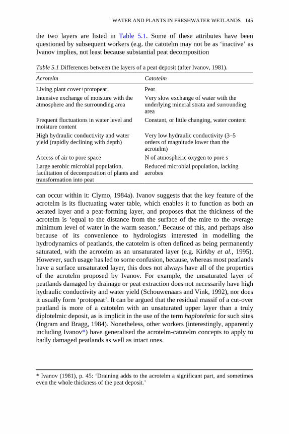
the two layers are listed in Table 5.1. Some of these attributes have beenquestioned by subsequent workers (e.g. the catotelm may not be as ‘inactive’ asIvanov implies, not least because substantial peat decomposition
Table 5.1 Differences between the layers of a peat deposit (after Ivanov, 1981).
Acrotelm Catotelm
Living plant cover+protopeat PeatIntensive exchange of moisture with theatmosphere and the surrounding area
Very slow exchange of water with theunderlying mineral strata and surroundingarea
Frequent fluctuations in water level andmoisture content
Constant, or little changing, water content
High hydraulic conductivity and wateryield (rapidly declining with depth)
Very low hydraulic conductivity (3–5orders of magnitude lower than theacrotelm)
Access of air to pore space N of atmospheric oxygen to pore sLarge aerobic microbial population,facilitation of decomposition of plants andtransformation into peat
Reduced microbial population, lackingaerobes
can occur within it: Clymo, 1984a). Ivanov suggests that the key feature of theacrotelm is its fluctuating water table, which enables it to function as both anaerated layer and a peat-forming layer, and proposes that the thickness of theacrotelm is ‘equal to the distance from the surface of the mire to the averageminimum level of water in the warm season.’ Because of this, and perhaps alsobecause of its convenience to hydrologists interested in modelling thehydrodynamics of peatlands, the catotelm is often defined as being permanentlysaturated, with the acrotelm as an unsaturated layer (e.g. Kirkby et al., 1995).However, such usage has led to some confusion, because, whereas most peatlandshave a surface unsaturated layer, this does not always have all of the propertiesof the acrotelm proposed by Ivanov. For example, the unsaturated layer ofpeatlands damaged by drainage or peat extraction does not necessarily have highhydraulic conductivity and water yield (Schouwenaars and Vink, 1992), nor doesit usually form ‘protopeat’. It can be argued that the residual massif of a cut-overpeatland is more of a catotelm with an unsaturated upper layer than a trulydiplotelmic deposit, as is implicit in the use of the term haplotelmic for such sites(Ingram and Bragg, 1984). Nonetheless, other workers (interestingly, apparentlyincluding Ivanov*) have generalised the acrotelm-catotelm concepts to apply tobadly damaged peatlands as well as intact ones.
* Ivanov (1981), p. 45: ‘Draining adds to the acrotelm a significant part, and sometimeseven the whole thickness of the peat deposit.’
WATER AND PLANTS IN FRESHWATER WETLANDS 145
The scope of the acrotelm concept is not just a matter of terminological nicetiesbut relates to the eco-hydrological function of this layer in peatlands. In a naturalombrogenous bog, the acrotelm layer may provide some hydrological regulation,dependent specifically upon properties such as high hydraulic conductivity andwater yield (Ivanov, 1981; Ingram, 1992; Joosten, 1993; Schouwenaars, 1996)that are not features of the aerated upper layer of a damaged catotelm. Thecombination of high hydraulic conductivity and high specific yield means thatthe acrotelm allows rapid dissipation of water excess (e.g. heavy rainfall,snowmelt) without a significant rise of water level. During drought the acrotelmmay shrink, bringing the mire surface closer to the water table. Ivanov (1981)suggests that these functions are hydroregulatory and thus provide a positivefeedback in which the plants that form the acrotelm help to produce conditionsappropriate for their continued growth. Such regulation may be especiallyimportant in ombrogenous peatlands, particularly for examples in regionssubjected to periods of drought (Joosten, 1993), although the magnitude andexact mechanisms of such postulated hydroregulation have yet to be establishedcritically. Sphagnum is particularly important to acrotelm hydroregulation onaccount of the loosely woven, expansible surface it often creates (Bragg, 1989),its capacity to store water (Romanov, 1968; Schouwenaars and Vink, 1992) andreduction of evapotranspiration by ‘mulching’ and albedo of bleached Sphagnum(Schouwenaars, 1990). Such hydroregulatory properties may be a particularfeature of spongy Sphagnum surfaces (Ingram, 1992; Joosten, 1993;Schouwenaars, 1996); it is not clear whether the acrotelm of bogs naturallydominated by graminoids (e.g. Eriopborum spp.) or tree species has acomparable capacity.
The hydrological importance of the acrotelm in fens is not well known. Fenshave a periodically unsaturated surface layer, but the depth of this can vary veryconsiderably and its hydroregulatory function remains to be established. It ispossible that Sphagnum-dominated poor fens may have a capacity forhydroregulation comparable to that of bogs (Ingram, 1992), but thehydrodynamics of many fens are controlled by external events independent ofany properties of their surface layers. For example, the stable water regimes ofsome soligenous fens may be imposed more by the constancy of spring flow thanby internal mechanisms, while in many other fens seasonal variation in rechargegenerates strongly fluctuating water levels. However, the upper layers of somelittle-modified rheo-topogenous fens may provide the main water flow pathsthrough the systems (Kulczynski, 1949; Succow, 1988).
Although the status and role of the acrotelm in fens is mostly uncertain, somefens do possess structures that provide some measure of hydrological self-regulation, created by vertically mobile mats of vegetation. These undoubtedlyrespond to variation in water supply and in some circumstances may help toregulate the hydrodynamics of the wetland.
146 ECO-HYDROLOGY
Vegetation rafts
While hydrologists are often particularly concerned with absolute water levels,the growth and distribution of wetland plants is related more to relative water levels(position of the water table relative to the soil surface, or to the rooting zone). Thisdistinction becomes important when the vegetation surface has some capacity forvertical mobility, as in vegetation rafts.
Vegetation rafts are perhaps most obviously associated with some types ofhydroseral colonisation of (usually small) water bodies, both in natural wetlandsand in reflooded turbaries (‘turf ponds’). However, raft-like surfaces have alsodeveloped in a range of other situations, and quaking, tremulous surfaces are afeature of many fens. Rafts vary enormously in their character and thickness,from thin skins of hydroseral vegetation formed from the entangled rhizomes ofhydrophytes growing over deep water and muds, to thick accumulations ofrelatively solid peat that have ‘broken away’ from lower layers of peat. Thethicker examples are generally the least mobile, and some rafts are groundedexcept at high water levels (e.g. Yabe and Onimaru, 1996).
Kulczynski (1949) paid particular attention to vegetation rafts and observedthat buoyant layers of peat frequently occur on top of heavier, solid peats, withvarying degrees of independence, sometimes separating only in high waterconditions. His so-called dysaptic structures consist of an admixture of tall plants(immersive perennials) rooting into a solid underlying layer of peat topped by abuoyant mat of semi-floating vegetation (Mörnsjö (1969) also provides somegood examples of this). The two layers may experience very differentenvironmental conditions. However, Kulczynski observed that the upper profilesof many fens did not show the contrasting layering of a dysaptic structure buthad a more uniform, unseparated profile in which the uppermost layers weregenerally less humified and which ‘undergo the biggest changes in their volumewhen the…water level oscillates.’ This cryptodysaptic structure—which iswidespread in many wet, topogenous fens — is more of an expandable peat massthan a true raft and has some obvious affinities with the acrotelm. Kulczynski(1949) emphasised that both cryptodysaptic and, especially, dysaptic structuresprovide an important water storage role that helps to reduce water level change.However, a buoyant raft also damps water level fluctuations relative to thevegetation on account of its mobility (Buell and Buell, 1941; Giller and Wheeler,1988; van Wirdum, 1991), and the key difference between a raft and an acrotelmis that whereas water levels fluctuate within an acrotelm, a mobile raft retains afairly stable position relative to the surface of a fluctuating water level. Ofcourse, vegetation rafts may also have an acrotelm in terms of a surfaceunsaturated layer that can presumably supplement or, as the raft thickens andsolidifies, supervene raft-based hydroregulation.
The hydroregulatory properties of rafts may explain their frequent associationwith a range of plant species that are either uncommon or unexpected (Giller andWheeler, 1986a, 1988; Den Held et al., 1992; Van Wirdum et al., 1992). For
WATER AND PLANTS IN FRESHWATER WETLANDS 147
example, some mobile rafts permit acidophiles such as Sphagnum spp. to growover very base-rich water, because their surface is rarely flooded (Giller andWheeler, 1988; van Wirdum, 1991). Yet other examples (in topogenous fens)support plant species that are particularly characteristic of soligenous situations(so-called ‘seepage indicator species’: Van Wirdum, 1991). Some workers haveattributed the occurrence of such species on vegetation rafts to the influence ofgroundwater discharge (Segal, 1966), but by no means all examples are indischarge areas (van Wirdum, 1991). The environmental features associated withvegetation rafts supporting ‘seepage indicator species’ in Britain and theNetherlands are base-rich, low-fertility water and a damped amplitude of waterlevel fluctuation (Giller and Wheeler, 1986a, b; van Wirdum, 1991). In theserespects, such vegetation rafts may mimic some salient characteristics of base-rich, soligenous fens without being subject to groundwater discharge.
WATER CHEMICAL COMPOSITION
In many wetlands, the inflowing water provides a major mechanism for the importof chemical elements. It helps to determine the availability of essential plantnutrients as well as regulating other components of the chemical environment ofthe rooting zone, such as pH. Variation in the chemical composition of watersources helps to control species distribution and vegetation composition inwetlands, and water quality can be of equal ecological importance to waterquantity. This should be recognised by water engineers and others who may betempted to remedy water deficit in a wetland by introducing supplementarywater of contrasting chemical composition to that of the original sources.
A large number of chemical studies have been made in wetlands (e.g. Malmer,1962a, b). Among their main foci have been characterisation of hydrochemicalconditions; identification of sources of water supply; examination andquantification of hydrochemical processes; and exploration of links betweenhydrochemistry and wetland vegetation. Various aspects of wetlandhydrochemistry have been reviewed by Shotyk (1988) and Ross (1995), amongothers. Here consideration will be restricted to some aspects of water chemistrythat are particularly pertinent to the distribution of plants and the composition ofwetland vegetation.
Vegetation-related gradients in the chemical compositionof water in wetlands
Trends in the chemical composition of water in wetlands
Gibbs (1970) has pointed out that the gross chemical composition of the world’ssurface waters is controlled by three main mechanisms: atmosphericprecipitation, supply from rocks and evaporation-crystallisation processes. He
148 ECO-HYDROLOGY
considers that it is possible to characterise the variation in surface waters usingjust two axes, the concentration of total dissolved salts and the ‘weight ratio’ .
Independently of Gibbs, van Wirdum (1982, 1991) developed a comparableapproach for representing the composition of water samples from wetlands. Heproposed that much of the variation in the chemical composition of wetland watercan be summarised as a two-dimensional ordination, where one axis is a measureof overall concentration as estimated by electrical conductivity (EC25) and thesecond is an estimate of ioni composition based on the quotient ‘IR’, where:
Van Wirdum (1991) found that most water samples plotted within a discrete, sub-triangular portion of the EC-IR ordination and that certain combinations of ECand IR were rare or absent. He concluded that the clusters of samples could becharacterised by reference to three more or less extreme points. These effectivelyform the apices of the sub-triangle and have been distinguished as:
• Lithotrophic: character derived from much contact with rocks (high IR,medium EC)
• Atmotrophic: character based on atmospheric water (low IR, low EC)• Thalassotrophic: character based on oceanic water (low IR, high EC)
This ‘LAT framework’ much simplifies the actual variation found in wetlandwater chemistry and provides a way of handling water samples for whichcomplete chemical analyses are not available (van Wirdum, 1991). It can providevaluable information about water sources and can correlate well with thedistribution of plant communities (Koerselman et al., 1990), suggesting that forsome purposes more detailed chemical determinations may be superfluous.
Working from a rather different perspective, Wheeler and Shaw (1995) made asynoptic comparison of the environmental conditions associated with fenvegetation in Britain and identified two primary gradients of vegetation-relatedchemical variation. The principal gradient was one of base richness and includedseveral closely correlated variables (positively related to base richness: Ca, Mg,HCO3; negatively related: pH, Fe, Mn, Al). The second gradient, orthogonal tothe first, was one of fertility.
The capacity of van Wirdum’s LAT framework to represent the distinctivecharacter of nutrient-enriched water is not fully established. Since ionscontaining N and P generally contribute rather little to electrical conductivity, itmay be suspected that nutrient-rich water may be difficult to detect in hisordination. Nonetheless, many forms of enrichment are associated withconcentration changes in solutes additional to growth-limiting nutrients, and vanWirdum (1991) has shown that polluted (molunotrophic) water occupies adistinctive position on the EC-IR plot, presumably on account of its overall ionicsignature.
WATER AND PLANTS IN FRESHWATER WETLANDS 149
The base-richness gradient
Variation in base richness of wetland waters corresponds broadly to theatmotrophic-lithotrophic gradient of the LAT framework and has long beenconsidered to be the primary gradient in relation to the floristic composition of mirevegetation (e.g. du Rietz, 1949; Sjörs, 1950a; Malmer, 1962a, 1986; Heinselman,1970; Wheeler and Shaw, 1995). The acidity of wetlands depends upon thecomposition of their water sources and upon their capacity to buffer acidityproduced endogenously by decomposition processes and protonation by plants,especially Sphagnum spp. (Clymo, 1984b; Shotyk, 1988).
Reflecting its importance to floristic composition, the base-richness gradienthas provided the basis for some of the main hydrochemical categories of wetlands.Du Rietz (1949, 1954) recognised the two main categories of bog and fen, withfen further subdivided into poor fen and rich fen. This classification is still quitewidely used, with its categories usually regarded as units of base status (in thesequence bog < poor fen < rich fen) (Sjörs, 1950a), although Du Rietz’s unitswere actually based on floristics, not on hydrological or hydrochemicaldefinitions. Bog and poor fen vegetation often has a prevalence of Sphagnum and,in general, is less species-rich than rich-fen vegetation of comparable lowproductivity.
The split between bog and fen corresponds—by definition—to an importantdifference in water source (exclusively meteoric versus telluric water-fedsystems), and the two categories are widely considered to be ‘fundamentalunits’. Nonetheless, they do not seem to represent the primary hydrochemical orfloristic subdivision of mires. The pH value of the water of natural mires rangesbetween the limits of about pH 2.5 and 9, but various workers have observed abimodal frequency distribution of water pH (Gorham et al., 1985; Proctor,1995). One mode (pH<5.0) appears to represent water buffered by humicmaterial; the other (pH > 6.0) represents water buffered by the bicarbonatesystem. The separating antimode (the point of ‘natural’ subdivision?)approximates quite closely to the split between rich fen and poor fen plus bog,not to the split between bog and fen (Malmer, 1986). Likewise, multivariatefloristic classifications of peatland vegetation do not necessarily identify bogversus fen as the primary split (Daniels, 1978; Gignac et al., 1991) but tend tosupport the approach of many European phytosociologists, who have generallygrouped bog vegetation together with much poor fen vegetation into a singleclass (Oxycocco-Sphagnetea Br.-Bl. et Tx. 1943). Thus, if there is any single‘natural’ subdivision within mires, it seems more likely to be fixed at rich fenversus the remainder rather than at bog versus fen.
In some peatlands, the base-rich to base-poor gradient is linked to ontogenicprocesses, especially to a diminishing influence of base-rich groundwater uponthe surface, often created by growth of plants (especially Sphagnum species)above the influence of base-rich water. Surface acidification can also be inducedby reduction of groundwater flow and the accumulation of lenses of rainwater in
150 ECO-HYDROLOGY
the upper peat, and thus drive floristic change rather than be the product of it.The importance of acid rain inputs to the base status and floristic composition ofwetlands is not at all well known. Although the effects of this might perhaps beexpected to be greatest in ombrogenous mires, which not only have a completedependence on precipitation inputs but which sometimes also occur in regions ofparticularly high total acid deposition, such systems are naturally of quite low pH(Proctor and Maltby, 1998). The most pervasive floristic consequences of acid rainare more likely to be upon high pH, but weakly buffered, wetlands (Kooijman,1993; Haesebroeck et al., 1997).
The fertility gradient
The productivity of wetlands shows enormous variation (Bradbury and Grace,1983), much of which is probably in response to variation in soil ‘fertility’. Thisis primarily controlled by the availability of growth-limiting nutrients, mainlynitrogen and phosphorus, sometimes potassium. In general, the most naturallyfertile wetlands occur alongside rivers, in areas subject to alluvial deposition—aprocess that may be encouraged by entrapment by vegetation. Fertile wetlands,at least when unmanaged, usually support robust, productive, species-poorvegetation dominated by one or a few vigorous, monopolistic species (e.g.Wheeler and Giller, 1982; Vermeer and Beredense, 1983; Wheeler and Shaw,1991). Very high concentrations of nutrients may be directly detrimental to themetabolism and growth of some wetland species, including potential dominantssuch as Phragmites australis (Kubín and Melzer, 1996; Votrubová andPechácková, 1996). Studies suggest that N, P and K availability can all limit plantgrowth in wetlands, although K limitation seems to be the least common. Someworkers have been particularly interested in identifying limiting nutrientsfor individual sites and vegetation types. Koerselman and Verhoeven (1995)tabulated examples of various European studies and concluded that bogs weremostly P-limited and fens mostly N-limited. However, this assessment maypartly reflect a preponderance of studies made in the Netherlands, because thereis plenty of evidence for P limitation in fens (e.g. Egloff, 1983; Richardson andMarshall, 1986; Boyer and Wheeler, 1989; Kooijman, 1993; Boeye et al., 1997).Moreover, the search for general patterns in the identity of limiting nutrients inwetlands may have only limited value. Hayati and Proctor (1991) presentevidence that the performance of different species can be influenced by differentnutrients, even on the same soil or site, with perhaps several nutrients being closeto their limiting concentrations; and that uptake of specific ions may beinfluenced by the presence of others. There is also some evidence thatavailability of N and P can influence the uptake of both elements (O’Connell andGrove, 1985; Perez-Corona and Verhoeven, 1996). If the availability of N helpsto control root phosphatase activity, so that increased N can relieve P deficiencyby stimulating hydrolysis of organic P sources, which element is then ‘limiting’?
WATER AND PLANTS IN FRESHWATER WETLANDS 151
Major nutrients may be imported into wetlands by inflowing water, fromnaturally or artificially enriched sources, but their availability can also beregulated by the position of the water table. Mineralisation processes are widelyconsidered to be much reduced by anoxia (although substantial N mineralisationhas been reported from some waterlogged soils: Williams and Wheatley, 1988).Conversely, denitrification occurs mostly in low-redox environments (< c. 300mV). It can, however, be rate-limited by insufficient nitrate flux, due inter alia toslow rates of nitrification and mineralisation or to limited penetration, orinsufficient residence, of nitrate-rich inflows in wetlands (Warwick and Hill,1988; Koerselman et al., 1989; Lowrance, 1992). Nonetheless, in appropriatecircumstances, especially given base-rich conditions and fluctuating watertables, denitrification can lead to loss of much N from wetlands (e.g. Guthrie andDuxbury, 1978; Reddy et al., 1980).
A variety of hydrochemical processes can help to regulate phosphorusavailability in wetlands. High water tables can be associated with an increase in Pavailability, probably largely on account of desorption processes (Koerselmanand Verhoeven, 1995). Conversely, in highly calcareous fens P can be adsorbedonto calcite precipitated in response to degassing of supersaturated groundwater(Boyer and Wheeler, 1989; Boeye et al., 1995). Some workers also point to Ca-Pimmobilisation through formation of hydroxyapatites (Kemmers, 1986), but thismechanism has sometimes been invoked for relatively low Ca concentrations,where its occurrence is far from certain (Wilson and Fitter, 1984; Wassen et al.,1989; Wassen and Barendregt, 1992).
Salinity gradients
In freshwater wetlands, outside the influence of marine or estuarine waters,salinity gradients are generally of little consequence. However, there can be agreater thalassotrophic influence in coastal freshwater systems, derived fromstorm surges that send periodic pulses of oligohaline water upstream and intowetlands (Giller and Wheeler, 1986b); from penetration of brackish groundwater(Wassen et al., 1989); and from ‘fossil salinity’ derived from former estuarinesediments now covered by freshwater deposits, especially where the surface ofestuarine clays has been exposed by peat removal (Giller and Wheeler, 1986a,b).
Relating water chemical composition to vegetationcomposition
While the vegetation composition of wetlands is undoubtedly strongly influencedby the chemical composition of water, the identification of exact chemical limitsfor particular plant species or communities has generally proved elusive. Someearly analyses of vegetation-hydrochemical relationships remain instructive.Gorham (1950) examined the hydrochemical boundary conditions of Carex
152 ECO-HYDROLOGY
lasiocarpa and concluded that they were very variable. Sjörs (1950a) observed aconsiderable inconsistency of association between measured chemicalconcentrations and plant distributions in between-site comparisons and notedthat, while some species showed the same rank order along hydrochemicalgradients at different sites, there could be great differences in actualconcentrations associated with them at each individual site. More recentworkers, optimistically trying to define coherent chemical conditions associatedwith species and communities, often do little more than confirm Gorham’s andSjörs’s observations about variability. Even when clear relationships areobserved at individual sites, they do not always have wider relevance. Forexample, Wassen et al. (1989) identified six broad water types in the fens in theNaardermeer (Netherlands), with clear correlations with species distribution, butthere is little reason to suppose that the species necessarily show the samehydrochemical ‘preferences’ and limits elsewhere. For example, in the UK suchspecies as Eupatorium cannabinum, Berula erecta and Lycopus europaeus donot seem to be preferentially associated with water with conductivities in excessof 700 µS cm−1 as observed by Wassen et al. (B.D.Wheeler and S.C.Shaw,unpublished data).
Difficulties of defining clear vegetation-hydrochemical relationships stempartly from the considerable spatial and temporal variation in water composition,even within the same stand (Malmer, 1962a; Summerfield, 1974; Proctor, 1994),sometimes associated with water level fluctuations (Giller and Wheeler, 1986b;Proctor, 1994). De Mars et al. (1997) report that the best correlation betweenwater composition in the root zones and vegetation types was found during verydry or very wet weather. Concentrations of ions in interstitial water do notnecessarily well reflect their bio-availability, especially those of growth-limitingnutrients, whose measured concentrations may be much determined bybiological uptake (e.g. Urban et al., 1988; Wheeler et al., 1992), or which occuras hydrolysable organic complexes.
Water sources, water chemistry and wetland vegetation
Since different water sources can have strikingly different chemical composition,changes in the proportionate contribution of contrasting sources may be expectedto affect the floristic composition of wetlands, even when there is no net changein water levels. In the Netherlands, some workers consider that flow of calcareousgroundwater, derived from adjoining upland recharge areas, is critical to theoccurrence of some of the more ‘desirable’ species and communities inwetlands. They also suggest that reduction of groundwater flow, or changingflow paths (induced by groundwater abstraction or drainage), can lead to adeterioration of floristic quality, even without a strong water level decrease, onaccount of an increased proportion of alternative water sources, such as nutrient-enriched land-drainage water or rainwater (Bakker et al., 1987; Grootjans et al.,1988; Van Diggelen et al., 1991a), and, in some situations, brackish groundwater
WATER AND PLANTS IN FRESHWATER WETLANDS 153
(Schot et al., 1988; Wassen et al., 1989). Because of this, there is much interestamong Dutch workers in identifying and maintaining (or reinstating) the regionalground water flow systems responsible for the production of the desiredhydrochemical conditions (Grootjans, 1985; Wassen et al., 1988; 1990; vanDiggelen et al., 1995).
Nonetheless, it is important to recognise that, from the point of view of plantgrowth and distribution, the chemical environment in the immediate vicinity ofthe plant is more critical than its mechanism of supply. Calcium-rich,mesotrophic water, in the Dutch fens and elsewhere, can originate from sourcesother than direct discharge of regional groundwater (van Wirdum, 1982; 1991;Wassen et al., 1990; Schot and Wassen, 1993). It can even have an artificialorigin (Boeye et al., 1995). Providing its quality is appropriate, plants may not‘mind’ too much from whence their water comes, or how it arrives! Thus, whilereinstatement of former regional flow patterns provides one importantmechanism for restoring appropriate hydrochemical conditions to wetland sites,it is not the only approach and should not obscure the possibility that similar, orequally desirable, floristic outcomes may be achieved by alternative supplymechanisms. For example, the fact that some rare ‘seepage indicator species’ cangrow on semi-floating vegetation rafts in reflooded peat workings that do notreceive any water ‘seepage’ (groundwater discharge) points to the possibilities ofmaintaining species populations in hydrological and hydrochemicalenvironments that do not correspond exactly to any former ‘natural condition’.Such opportunities need to be identified and grasped, because in some highlydeveloped landscapes provision of ‘new’ environments and hydrologicalmechanisms may offer the only realistic prospect for wetland restoration. Suchan approach does, however, demand a more thorough understanding of theinterrelationships between hydrology and hydrochemistry and vegetationcomposition than currently exists.
ACKNOWLEDGEMENTS
I thank H.A.P.Ingram, P.A.Keddy, R.P.Money, M.C.F.Proctor, S.C.Shaw and G.van Wirdum for helpful comments on an early draft of this paper. N.Malmermade some valuable comments on the importance of the acrotelm in fens.J.Schouwenaars contributed material on eco-hydrological models used in theNetherlands.
REFERENCES
Andrus, R.E. (1986) Some aspects of Sphagnum ecology, Canadian Journal of Botany64:416–426.
154 ECO-HYDROLOGY
Andrus, R.E., Wagner, D.J. and Titus, J.E. (1983) Vertical distribution of Sphagnummosses along hummock-hollow gradients, Canadian Journal of Botany 61:3128–3189.
Armstrong, J., Armstrong, W. and Beckett, P.M. (1992) Phragmites australis: venturi-and humidity-induced pressure flows enhance rhizome aeration and rhizosphereoxidation, New Phytologist 120:197–202.
Armstrong, J., Armstrong, W., Wu, Z. and Afreen-Zobayed, F. (1996) A role forphytotoxins in the Phragmites die-back syndrome? Folia Geobotanica andPhytotaxonomica 31:127–142.
Armstrong, W. (1964) Oxygen diffusion from the roots of some British bog plants, Nature204:801–802.
Armstrong, W. (1967) The oxidising activity of roots in waterlogged soils, PhysiologiaPlantarum 20:920–926.
Armstrong, W. (1980) Aeration in higher plants, Advances in Botanical Research 7:226–332.
Armstrong, W. (1982) Waterlogged soils, in J.R.Etherington (ed.) Environment and PlantEcology, second edition, Chichester: John Wiley, pp. 290–330.
Armstrong, W. and Boatman, D.J. (1967) Some field observations relating the growth ofbog plants to conditions of soil aeration, Journal of Ecology 55: 101–110.
Armstrong, W., Armstrong, J. and Beckett, P.J. (1996) Pressurised aeration in wetlandmacrophytes: some theoretical aspects of humidity-induced convection and thermaltranspiration, Folia Geobotanica and Phytotaxonomica 31:25–36.
Armstrong, W., Booth, T.C., Priestley, P. and Read, D.J. (1976) The relationship betweenaeration, stability and growth of Sitka spruce (Picea sitchensis (Bong.) Carr.) onupland peaty gleys, Journal of Applied Ecology 13:585–591.
Bakker, J.P., Brouwer, C., van den Hof, L. and Jansen, A. (1987) Vegetation succession,management and hydrology in a brookland (The Netherlands), Acta BotanicaNeerlandica 36:39–58.
Balátová-Tulácková, E. (1968). Grundwasserganglinien und Wissengesellschaften(Vergleichende Studie der Wiesen aus Südmähren und der Südwestslowakei), ActaScientiarum Naturalium Academiae Scientiarum Bohemoslovacae Brno 2:1–37.
Barclay, A.M. and Crawford, R.M.M. (1982) Plant growth and survival under strictannerobiosis, Journal of Experimental Botany 33:541–549.
Barendregt, A., Wassen, M.J., de Smidt J.T. and Lippe, E. (1986) Ingreep effectvoorspelling voor waterbeheer, Landschap 3:41–55.
Bartlett, R.J. (1961) Iron oxidation proximate to plant roots, Soil Science 92: 372–379.Baskin, C.C., Baskin, J.M. and Chester, E.W. (1993) Seed germination eco-physiology of
four summer annual mudflat species of Cyperaceae, Aquatic Botany 45:41–52.Bedford, B.L. and Bouldin, D.R. (1994) ‘On the difficulties of measuring oxygen release
by root systems of wetland plants’, by B.K.Sorrell and W.Armstrong, Journal ofEcology 82:185–186.
Bedford, B.L., Bouldin, D.R. and Beliveau, B.D. (1991) Net oxygen and carbon dioxidebalances in solutions bathing roots of wetland plants, Journal of Ecology 79:943–959.
Beets, C.P. (1992) The relation between the area of open water in bog remnants andstorage capacity with resulting guidelines for bog restoration, in O.M.Bragg,P.D.Hulme, H.A.P.Ingram and R.A.Roberstson (eds) Peatland Ecosystems and Man:
WATER AND PLANTS IN FRESHWATER WETLANDS 155
An Impact Assessment, University of Dundee: Dundee/International Peat Society:Jyväskylä, pp. 133–140.
Bellamy, D.J. (1968) An ecological approach to the classification of European mires,Third International Peat Congress, Quebec 1968, pp. 74–79.
Bellamy, D.J. and Bellamy, S.R. (1966) An ecological approach to the classification ofthe lowland mires of Ireland, Proceedings of the Royal Irish Academy B65:237–251.
Bewley, J.D., Halmer, P., Krochko, J. and Winner, W.E. (1978). Metabolism of a drought-tolerant and a drought-sensitive moss. Respiration, ATP synthesis and carbohydratestatus, in J.H.Crowe and J.S.Clegg (eds) Dried biological systems, New York:Academic Press, pp. 185–203.
Blom, C.P.W.M., Voesenek, L.A.C.J., Banga, M., Engelaar, W.M.H.G., Rijnders,J.H.M.G., van Steeg, H.M. and Visser, E.J.W. (1994) Physiological ecology ofriverside species, adaptive responses upon submergence, Annals of Botany 74:253–263.
Bloomfield, C. and Zahari, A.B. (1982) Acid sulphate soils, Outlook on Agriculture 11:48–54.
Boeye, D., van Straaten, D. and Verheyen, F. (1995) A recent transformation from poor torich fen caused by artificial ground water recharge, Journal of Hydrology 169:111–129.
Boeye, D., Verhagen, B., van Haeseboroeck, V. and Verheyen, R.F. (1997) Nutrientlimitation in species-rich lowland fens, Journal of Vegetation Science 8:415–424.
Boyer, M.H.L. and Wheeler, B.D. (1989) Vegetation patterns in spring-fed calcareousfens: calcite precipitation and constraints on fertility , Journal of Ecology 77:597–609.
Bradbury, I.K. and Grace, J. (1983) Primary production in wetlands, in A.J.P.Gore (ed.)Ecosystems of the World. 4A. Mires: Swamp, Bog, Fen and Moor. General Studies,Amsterdam: Elsevier, pp. 285–310.
Braendle, R. and Crawford, R.M.M. (1987) Rhizome anoxia tolerance and habitatspecialization in wetland plants, in R.M.M.Crawford (ed.) Plant Life in Aquatic andAmphibious Habitats, Oxford: Blackwell Scientific Publications, pp. 397–410.
Bragg, O.M. (1989). The importance of water in mire ecosystems, in W.Fojt and R.Meade(eds) Cut-over Lowland Raised Mires, Peterborough, Research and Survey in NatureConservation 24, Nature Conservancy Council, pp. 61–82.
Buell, M.F. and Buell, H.F. (1941) Surface level fluctuations in Cedar Creek Bog,Minnesota, Ecology 22:314–321.
Chapin, F.S., Fetcher, N., Kielland, K., Everett, K.R. and Linkins, A.E. (1988)Productivity and nutrient cycling of Alaskan tundra: enhancement by flowing soilwater, Ecology 69:693–702.
Clapham, A.R. (1940) The role of bryophytes in the calcareous fens of the Oxforddistrict, Journal of Ecology 28:71–80.
Clausen, E. (1952) Hepatics and humidity, a study on the occurrence of hepatics in aDanish tract and the influence of relative humidity on their distribution, Dan. Bot.Ark. 15:5–80.
Clymo, R.S. (1970) The growth of Sphagnum: methods of measurement, Journal ofEcology 58:13–49.
Clymo, R.S. (1973) The growth of Sphagnum: some effects of environment, Journal ofEcology 61:849–869.
156 ECO-HYDROLOGY
Clymo, R.S. (1984a) The limits to peat bog growth, Philosophical Transactions of theRoyal Society of London B303:605–654.
Clymo, R.S. (1984b) Sphagnum-dominated peat bog: a naturally acid ecosystem,Philosophical Transactions of the Royal Society of London B305:487–499.
Clymo, R.S. and Reddaway, E.J.F. (1971) Productivity of Sphagnum (bog moss) and peataccumulation, Hidrobiologia 12:181–192.
Clymo, R.S. and Hayward P.M. (1982) The ecology of Sphagnum, in A.J.E.Smith (ed.)Bryophyte Ecology, London: Chapman and Hall, pp. 229–291.
Conway, V.M. (1937) Studies in the autecology of Cladium mariscus R. Br. Part III. Theaeration of the subterranean parts of the plant, New Phytologist 36:64–96.
Conway, V.M. (1938) Studies in the autecology of Cladium mariscus R. Br. IV. Growthrates of the leaves, New Phytologist 37:254–278.
Conway, V.M. (1940) Growth rates and water loss in Cladium mariscus R. Br., Annals ofBotany 4:151–164.
Coops, H., van den Brink, F.W.B. and van der Velde, G. (1996) Growth andmorphological response of four helophyte species in an experimental water depthgradient, Aquatic Botany 54:11–24.
Coops, H. and van der Velde, G. (1995) Dispersal, germination and seedling growth of sixhelophyte species in relation to waterlevel zonation, Freshwater Biology 34: 13–20.
Crawford, R.M.M. (1977) Tolerance of anoxia and ethanol metabolism in germinatingseeds, New Phytologist 79:511–517.
Crawford, R.M.M. (1983) Root survival in flooded soils, in A.J.P.Gore (ed.) Ecosystemsof the World. 4A. Mires: Swamp, Bog, Fen and Moor. General Studies, Amsterdam:Elsevier, pp. 257–283.
Crawford, R.M.M. (1996) Whole plant adaptations to fluctuating water tables, FoliaGeobotanica Phytotaxonomia 31:7–24.
Daniels, R.E. (1978) Floristic analyses of British mires and mire communities, Journal ofEcology 66:773–802.
Daniels, R.E. and Pearson, M.C. (1974) Ecological studies at Roydon Common, Norfolk,Journal of Ecology 62:127–150.
de Mars, H. (1996) Chemical and Physical Dynamics of Fen Hydro-ecology, NederlanseGeografische Studies 203, Koninklijk Nederlands Aardrijkskundig Genootschap/Faculteit Ruimtelijke Wetenschappen Universiteit Utrecht,
de Mars, H., Wassen, M.J. and Olde Venterink, H. (1997) Flooding and ground waterdynamics in fens in the Biebrza Valley, N.E.Poland, Journal of Vegetation Science8: 19–328.
den Held, A.J., Schmitz, M. and van Wirdum, G. (1992) Types of terrestrializing fenvegetation in the Netherlands, in J.T.A.Verhoeven (ed.) Fens and Bogs in theNetherlands Dordrecht: Kluwer, pp. 237–322.
Drew, M.C., Sisworo, E.J. and Saker, L.R. (1979) Alleviation of waterlogging damage toyoung barley plants by application of nitrate and synthetic cytokinin and comparisonbetween the effects of waterlogging, nitrogen deficiency and root excision, NewPhytologist 82:315–329.
du Rietz, G.E. (1949) Huvudenheter och granser i Svensk myrvegetation, Svensk BotaniskTidskrift 43:299–309.
du Rietz, G.E. (1954) Die Mineralbodenwasserzeigergrenze als Grundlage einerNatürlichen Zwiegleiderung der Nord- und Mitteleuropäischen Moore, Vegetatio 5–6:571–585.
WATER AND PLANTS IN FRESHWATER WETLANDS 157
Eades, P.A. (1997) Experimental studies into the effects of water level changes upon thevegetation and fertility of calcareous spring-fed fens, unpublished PhD thesis,University of Sheffield.
Egloff, T. (1983) Der Phosphor als primär limitierender Nährstoff im Streuwiesen(Molinion). Düngungsexperiment im unteren Reusstal, Ber. Geobot. Inst. Eidg,Tech. Hochsch. Stuft. Rübel Zürich 50:119–148.
Egloff, T. and Naef, E. (1982) Grundwasserstandsmessungung in Streuwiesen des unterenReußtales, Ber. Geobot. Inst. ETH, Stiftung Rübel 49:154–194.
Ellenberg, H. (1954) Über einige Fortschritte der kausalen Vegetationskunde, Vegetatio 5–6:199–211.
Ellenberg, H. (1974) Zeigerwerte der Gefaßpflanzen Mitteleuropas, Scripta Geobotanica9:1–97.
Ellenberg, H. (1988) Vegetation Ecology of Central Europe, fourth edition, Cambridge:Cambridge University Press.
Engelaar, W.M.H.G., Symens, J.C., Laanbroeck, H.J. and Blom, C.W.P.M. (1995)Preservation of nitrifying capacity and nitrate availability in waterlogged soils byradial oxygen loss from the roots of wetland plants, Biology and Fertility of Soils 20:243–248.
Ernst, W.H.O. and van der Ham, N.F. (1988) Population structure and rejuvenationpotential of Schoenus nigricans in coastal dune slacks, Acta Botanica Neerlandica37: 451–465.
Etherington, J.E. (1984) Comparative studies of plant growth and distribution in relationto waterlogging. X. Differential formation of adventitious roots and theirexperimental excision in Epilobium hirsutum and Chamerion angustifolium, Journalof Ecology 72:389–404.
Evans, C.E. and Etherington, J.R. (1991) The effect of soil water potential on seedlinggrowth of some British plants, New Phytologist 118:571–580.
Fojt, W. and Harding, M. (1995) Thirty years of change in the vegetation communities ofthree valley mires in Suffolk, England, Journal of Applied Ecology 32: 561–577.
Fürtig, K., Rüegsegger, A., Brunold, C. and Brändle, R. (1996) Sulphide utilization andinjuries in hypoxic roots and rhizomes of common reed (Phragmites australis), FoliaGeobotanica and Phytotaxonomica 31:143–151.
Gibbs, R.J. (1970) Mechanisms controlling world water chemistry, Science 170:1088–1090.
Gignac, L.D., Vitt, D.H., Zoltai, S.C. and Bayley, S.E. (1991) Bryophyte responsesurfaces along climatic, chemical and physical gradients in peatlands of westernCanada, Nova Hedwigia 53:27–71.
Gill, C.J. (1970) The flooding tolerance of woody species—a review, Forestry Abstracts31:671–678.
Gill, C.J. (1975) The ecological significance of adventitious rooting as a response toflooding in woody species, with special reference to Alnus glutinosa (L.) Gaertn.,Flora 164:85–97.
Giller, K.E. and Wheeler, B.D. (1986a) Past peat cutting and present vegetation patternsin an undrained fen in the Norfolk Broadland, Journal of Ecology 74: 219–247.
Giller, K.E. and Wheeler, B.D. (1986b) Peat and peat water chemistry of a flood-plain fenin Broadland, Norfolk, UK, Freshwater Biology 16:99–114.
Giller, K.E. and Wheeler, B.D. (1988) Acidification and succession in a flood-plain mirein the Norfolk Broadland, UK, Journal of Ecology 76:849–866.
158 ECO-HYDROLOGY
Godwin, H. and Bharucha, F.R. (1932) Studies in the ecology of Wicken Fen. II. The fenwater table and its control on plant communities, Journal of Ecology 20: 157–191.
Gorham, E. (1950) Variation in some chemical conditions along the borders of a Carexlasiocarpa fen community, Oikos 2:217–240.
Gorham, E., Eisenreich, S.J., Ford, J. and Santelmann, M.V. (1985) The chemistry of bogwaters, in W.Stumm (ed.) Chemical Processes in Lakes, New York: Wiley,pp. 339–363.
Grace, J.B. and Wetzel, R.G. (1981) Habitat partitioning and competitive displacement incattails (Typha): experimental field studies, The American Naturalist 118:463–474.
Gremmen, N.J.M., Reignen, M.J.S.M., Wiertz, J. and van Wirdum, G. (1990) A model topredict and assess the effects of ground-water withdrawal on vegetation in thePleistocene areas of the Netherlands, Journal of Environmental Management 31:143–155.
Grootjans, A.P. (1980) Distribution of plant communities along rivulets in relation tohydrology and management, in O.Wilmanns and R.Tüxen (eds) Epharmonie.Berichte über die internationalen Symposien der Internationale Vereinigung fürVegetationskunde 1979, Cramer Verlag, pp. 143–170.
Grootjans, A.P. (1985) Changes of ground water regime in wet meadows, PhD thesis,University of Groningen.
Grootjans, A.P. and Ten Klooster, W.P. (1980) Changes of ground water regime in wetmeadows, Acta Botanica Neerlandica 29:541–554.
Grootjans, A.P., Fresco, L.F.M., de Leeuw, C.C. and Schipper, P.C. (1996) Degenerationof species-rich Calthion palustris hay meadows; some considerations on thecommunity concept, Journal of Vegetation Science 17:185–194.
Grootjans, A.P., van Diggelen, R., Wassen, M.J. and Wiersinga, W.A. (1988) The effectsof drainage upon ground water quality and species distribution in stream valleymeadows, Vegetatio 75:37–48.
Guthrie, T.F. and Duxbury, J.M. (1978) Nitrogen mineralisation and denitrification inorganic soils, Soil Science Society of America Journal 42:908–912.
Hacker, S.D. and Berness, M.D. (1995) Morphological and physiological consequences ofa positive plant interaction, Ecology 76:2165–2175.
Haesebroeck, V., Boeye, D., Verhagen, B. and Verheyen, R.F. (1997) Experimentalinvestigation of drought induced acidification in a rich fen soil, Biogeochemistry 37:15–32.
Hansen, J.I. and Andersen, P.O. (1981) Effects of Phragmites australis roots on redoxpotentials, nitrification and bacterial numbers in sediments, in A.Bromberg andT.Tiren (eds) Ninth Nordic Symposium on Sediments, pp. 72–78.
Harris, S.W. and Marshall, W.H. (1963) Ecology of water level manipulations on anorthern marsh, Ecology 44:331–343.
Haukos, D.A. and Smith, L.M. (1993) Seed-bank composition and predictive ability of fieldvegetation in playa lakes, Wetlands 13:32–40.
Hayati, A.A. and Proctor, M.C.F. (1991) Limiting nutrients in acid-mire vegetation: peatand plant analyses and experiments on plant responses to added nutrients, Journal ofEcology 79:75–95.
Hayward, P.M. and Clymo, R.S. (1983) The growth of Sphagnum—experiments on, andsimulation of, some effects of light flux and water table depth, Journal of Ecology 71:845–863.
WATER AND PLANTS IN FRESHWATER WETLANDS 159
Heikkilä, R. and Löytönen, M. (1987) Observations on Sphagnum species and theirrelation to vegetation and ecological factors in Ostanberg Stormossen, SouthFinland, Suo 38:63–70.
Heinselman, M.L. (1970) Landscape evolution, peatland types and the environment in theLake Agassiz Peatlands Natural Area, Minnesota, Ecological Monographs 40:236–261.
Hill, N.M. and Keddy, P.A. (1992) Prediction of rarities from habitat variables: coastalplain plants on Nova Scotian lakeshores, Ecology 73:1852–1859.
Hulme P.D. and Blyth A.W. (1982) The annual growth period of some Sphagnum specieson the Silver Flowe National Nature Reserve, south-west Scotland, Journal ofBryology 12:287–291.
Huisman, J., Olff, H. and Fresco, L.F.M. (1993) A hierarchical set of models for speciesresponse analysis , Journal of Vegetation Science 4:47–56.
Hygen, G. (1953) Studies in Plant Transpiration. II, Physiologia Plantarum 6: 106–133.Ingold, A. and Havill, D.C. (1984) The effect of sulphide on the distribution of higher
plants in salt marshes, Journal of Ecology 72:1043–1054.Ingram, H.A.P. (1967) Problems of hydrology and plant distribution in mires, Journal of
Ecology 55:711–724.Ingram, H.A.P. (1982) Size and shape in raised mire ecosystems: a geophysical model,
Nature 297:300–303.Ingram, H.A.P. (1992) Introduction to the ecohydrology of mires in the context of cultural
perturbation, in O.M.Bragg, P.D.Hulme, H.A.P.Ingram and R.A. Roberstson (eds)Peatland Ecosystems and Man: An Impact Assessment, University of Dundee:Dundee/International Peat Society: Jyväskylä, pp. 67–93.
Ingram, H.A.P. and Bragg, O.M. (1984) The diplotelmic mire: some hydrologicalconsequences reviewed, Proceedings of the 7th International Peat Congress, Dublin,June, 1984. Irish National Peat Committee, for the International Peat Society 1:220–234.
Ivanov, K.E. (1981) Water Movement in Mirelands, trans. A.Thomson and H.A.P. Ingram,London: Academic Press.
Jeglum, J.K. (1971) Plant indicators of pH and water level in peatlands at Candle Lake,Saskatchewan, Canadian Journal of Botany 49:1661–1676.
Johnson, W.C. (1994) Woodland expansion in the Platte River, Nebraska: patterns andcauses, Ecological Monographs 64:45–84.
Jones, H.E. (1972) Comparative studies of plant growth and distribution in relation towaterlogging. V. The uptake of iron and manganese by dune and dune slack plants,Journal of Ecology 60:131–140.
Jones, H.E. and Etherington, J.R. (1970) Comparative studies of plant growthand distribution in relation to waterlogging. I. The survival of Erica cinerea L. andErica tetralix L. and its apparent relationship to iron and manganese uptake inwaterlogged soil, Journal of Ecology 58:487–496.
Joosten, H.J. (1993) Denken wie ein Hochmoor: Hydrologische Selbsregulation vonHochmooren und deren Bedeutung für Wiedernässung und Restauration, Telma 23:95–115.
Justin, S.H.F.W. and Armstrong, W. (1987) The anatomical characteristics of roots andplant response to soil flooding, New Phytologist 106:465–495.
Kadlec, J.A. (1962) Effects of a drawdown on a waterfowl impoundment, Ecology 43:1443–1457.
160 ECO-HYDROLOGY
Kausch, A.P., Seago, J.L. and Marsh, L.C. (1981) Changes in starch distribution in theoverwintering organs of Typha latifolia (Typhaceae), American Journal of Botany68:877–880.
Keddy, P.A. (1983) Shoreline vegetation in Axe Lake, Ontario: Effects of exposure onzonation patterns, Ecology 64:331–344.
Keddy, P.A. (1989) Effects of competition from shrubs on herbaceous wetland plants: a 4-year experiment, Canadian Journal of Botany 67:708–716.
Keddy, P.A. and Constabel, P. (1986) Germination often shoreline plants in relation toseed size, soil particle size and water level: an experimental study, Journal ofEcology 74:133–141.
Keddy, P.A. and Ellis, T.H. (1985) Seedling recruitment of 11 plant species along a waterlevel gradient: shared or distinct responses?, Canadian Journal of Botany 63:1876–1879.
Keddy, P.A. and Reznicek, A.A. (1982) The role of seedbanks in the persistence ofOntario’s coastal plain flora, American Journal of Botany 69:13–22.
Keddy, P.A., Twolan-Strutt, L. and Wisheu, I.C. (1994) Competitive effect and responserankings in 20 wetland plants: are they consistent across three environments?Journal of Ecology 82:635–643.
Keeley, J.E. (1979) Population differentiation along a flood frequency gradient:physiological adaptations to flooding in Nyssa sylvatica, EcologologicalMonographs 49:89–108.
Kemmers, R.H. (1986) Calcium as hydrochemical characteristic for ecological states,Institute for Land and Water Management Research (ICW), Wageningen, theNetherlands. Technical Bulletin, ICW New Series 47:1–16.
Kirkby, M.J., Kneale, P.E., Lewis, S.L. and Smith, R.T. (1995) Modelling the form anddistribution of peat mires, in J.M.R.Hughes and A.L.Heathwaite (eds) Hydrology andHydrochemistry of British Wetlands. Chichester: John Wiley, pp. 83–93.
Klimesova, J. (1994) The effects of timing and duration of floods on growth of youngplants of Phalaris arundinacea L. and Urtica dioica L.: an experimental study,Aquatic Botany 48:21–29.
Klötzli, F. (1969) Die Grundwasserbeziehungen der Streu- und Moorwiesen imnördlichen Schweizer Mitteland, Beitrag geobot. Landesaufnahme 52:1–296.
Koerselman, W. and Verhoeven, J.T.A. (1995) Eutrophication of fen ecosystems: externaland internal nutrient sources and restoration strategies, in B.D.Wheeler, S.C.Shaw,W.J.Fojt and R.A.Robertson (eds) Restoration of Temperate Wetlands, Chichester:Wiley, pp. 91–112.
Koerselman, W., de Caluwe, H. and Kieskamp, W. (1989) Denitrification and dinitrogenfixation in two quaking fens in the Vechtplassen area, the Netherlands,Biogeochemistry 8:153–165.
Koerselman, W., Claessens, D., ten Den, P. and van Winden, E. (1990) Dynamichydrochemical and vegetation gradients in fens, Wetlands Ecology and Management1:73–84.
Koncalová, H., Kvet, J. Pokorny, J. and Hauser, V. (1993) Effect of flooding with sewagewater on three wetland sedges, Wetlands Ecology and Management 2: 199–211.
Kooijman, A. (1993) Changes in the bryophyte layer of rich fens as controlled byacidification and eutrophication, doctoral thesis, Universiteit Utrecht.
WATER AND PLANTS IN FRESHWATER WETLANDS 161
Kotowski, W., van Diggelen, R. and Kleinke, J. (in press) On the consistency of therealised niches of plants—comparison of wetland species behaviour in twogeographically distant areas , Acta Botanica Neerlandica.
Kozlowski, T.T. (ed.) (1984) Flooding and Plant Growth, Orlando, Fla.: Academic Press.Kramer, P.J. (1969) Plant and Soil Water Relationships, New York: McGraw-Hill.Kubín, P. and Melzer, A. (1996) Does ammonium affect accumulation of starch in rhizomes
of Phragmites australis? Folia Geobotanica and Phytotaxonomica 31:99–109.Kulczynski, S. (1949) Peat bogs of Polesie, Mémoires de l’académie Polonaise des
Sciences et des Lettres, Serie B: Science Naturelles 15:1–356.Laan, P., Smolders, A., Blom, C.W.P.M. and Armstrong, W. (1989) The relative roles of
internal aeration, radial oxygen loss, iron exclusion and nutrient balances in floodtolerance of Rumex species, Acta Botanica Neerlandica 38:131–145.
Lambert, J.M. (1951) Alluvial stratigraphy and vegetational succession in the region ofthe Bure valley broads. III. Classification, status and distribution of communities,Journal of Ecology 39:149–170.
Lane, D.M. (1977) Extent of vegetative reproduction in eleven species of Sphagnum fromnorthern Michigan, Michigan Botanist 16:83–89
Latour, J.B., Reiling, R.J. and Wiertz, J. (1993) MOVE; a multiple stress model for thevegetation, Proceedings of the CHO-TNO Symposium Ecohydrologischevoorspellingsmodellen, 25 May 1993. CHO-TNO 47, Delft.
Lee, J.A. and Stewart, G.R. (1971) Desiccation injury in mosses. I. Intra-specificdifferences in the effect of moisture stress on photosynthesis, New Phytologist 70:1061–1068.
Li, Y., Glime J.M. and Liao, C. (1992). Responses of two interacting Sphagnum species towater level, Journal of Bryology 17:59–70.
Lowrance, R. (1992) Ground water nitrate and denitrification in a coastal plain riparianforest, Journal of Environmental Quality 21:401–405.
Luken J.O. (1985) Zonation of Sphagnum mosses: interaction among shoot growth,growth form and water balance, The Bryologist 88:374–379.
Maas, D. (1989) Germination characteristics of some plant species from calcareous fensin southern Germany and their implications for the seed bank, Holarctic Ecology 12:337–344.
Maas, D. and Schopp-Guth, A. (1995) Seed banks in fen areas and their potential use inrestoration ecology, in B.D.Wheeler, S.C.Shaw, W.J.Fojt and R.A. Robertson (eds)Restoration of Temperate Wetlands. Chichester: Wiley, pp. 189–206.
MacMannon, M. and Crawford, R.M.M. (1971) A metabolic theory of flooding tolerance:the significance of enzyme distribution and behaviour, New Phytologist 70:299–306.
Malmer, N. (1962a) Studies on mire vegetation in the Archaean area of southwesternGötaland (south Sweden). I. Vegetation and habitat conditions on the Åkuhlt mire,Opera Botanica 7:1–322.
Malmer, N. (1962b) Studies on mire vegetation in the Archaean area of southwesternGötaland (south Sweden). II. Distribution and seasonal variation in elementaryconstituents on some mire sites, Opera Botanica 7:1–67.
Malmer, N. (1968) Über die Gliederung der Oxycocco-Sphagnetea und Scheuchzerio-Caricetea fuscae, in R.Tüxen (ed.) Planzensoziologische Systematik. Bericht überdas internationale Symposium in Stolenzau/Weser 1964 der InternationalenVereinigung für Vegetationskunde, Den Haag: Junk, pp. 293–305.
162 ECO-HYDROLOGY
Malmer, N. (1986) Vegetation gradients in relation to environmental conditions innorthwestern European mires, Canadian Journal of Botany 64:3750383.
Mansfield, S.M. (1990) Ecophysiological effects of high concentrations of iron and otherheavy metals on Eriophorum angustifolium Honck and Phragmites australis (Cav.)Trin. ex Steudel, unpublished PhD thesis, University of Sheffield.
Metsävainio, K. (1931) Untersuchungen über das Wurzelsystem der Moorpflanzen, Ann.bot. soc. zool.-bot. fenn. Vanamo 1.
Miles, J. (1976) The growth ofNarthecium ossifragum in some southern English mires,Journal of Ecology 64:849–858. Mitsch, W.J. and Gosselink, J.G. (1986) Wetlands,New York: Van Nostrand Reinhold.
Mooney, E.P. and O’Connell, M. (1990) The phytosociology and ecology of the aquaticand wetland plant communities of the lower Corrib basin, County Galway,Proceedings of the Royal Irish Academy 90B:57–97.
Mörnsjö, T. (1969) Studies on vegetation and development of a peatland in Scania, SouthSweden, Opera Botanica 24:1–187.
Mountford, J.O. and Chapman, J.M. (1993) Water regime requirements of British wetlandvegetation: using the moisture classifications of Ellenberg and Londo, Journal ofEnvironmental Management 38:275–288.
Murkin, H.R. and Ward, P. (1980) Early spring cutting to control cattail in a northernmarsh, Wildlife Socety Bulletin 8:254–256.
Newbould, C. and Mountford, O. (1997) Water Level Requirements of Wetland Plantsand Animals, English Nature Freshwater Series No. 5, Peterborough: English Nature.
Niemann, E. (1963) Beziehungen zwischen Vegetation and Grundwasser, Archiv fürNaturschutz und Landschaftsforschung 3:3–37.
Niemann, E. (1973) Grundwasser und Vegetationsgefüge, Nova Acta Leopold 6: 1–147.Nilsson, C. and Keddy, P.A. (1988) Predictability of change in shoreline vegetation in a
hydroelectric reservoir, northern Sweden, Canadian Journal of Fisheries andAquatic Sciences 45:1896–1904.
Noest, V. (1994) A hydrology-vegetation interaction model for prediction of theoccurrence of plant species in dune slacks, Journal of Environmental Management40: 119–128.
O’Connell, A.M. and Grove, T.S. (1985) Acid phosphatase activity in karri in relation tosoil phosphate and nitrogen supply, Journal of Experimental Botany 36: 1359–1372.
Olff, H., Berendse, F., Verkaar, D. and van Wirdum, G. (1995) Modelling vegetationsuccession , Landschap 12:69–82.
Osborne, D.J. (1984). Ethylene and plants of aquatic and semi-aquatic environments. Areview, Plant Growth Regulation 2:167–185.
Pakarinen, P. (1978) Production and nutrient ecology of three Sphagnum species insouthern Finnish raised bogs, Annales Botanici Fennici 15:15–26.
Patrick, W.H. and DeLaune, R.D. (1972) Characterisation of the oxidised and reducedzones in flooded soil, Soil Science Society of America, Proceedings 36:573–576.
Pearsall, W.H. (1938) The soil complex in relation to plant communities. I. Oxidation-reduction potentials in soils, Journal of Ecology 26:180–193.
Pedersen, A. (1975) Growth measurements of five Sphagnum species in south Norway,Norwegian Journal of Botany 22:277–284.
Perez-Corona, M.E. and Verhoeven, J.T.A. (1996) Effects of soil P status on growth and Pand N uptake of Carex species from fens differing in P availability, Acta BotanicaNeerlandica 45:381–392.
WATER AND PLANTS IN FRESHWATER WETLANDS 163
Poiani, K.A. and Johnson, W.C. (1989) Effect of hydroperiod on seedbank composition insemipermanent prairie wetlands, Canadian Journal of Botany 67: 856–864.
Ponnamperuma, F.N. (1972) The chemistry of submerged soils, Advances in Agronomy24:29–96.
Poschlod, P. (1995) Diaspore rain and diaspore bank in raised bogs and implications forthe restoration of peat-mined sites, in B.D.Wheeler, S.C.Shaw, W.J.Fojt andR.A.Robertson (eds) Restoration of Temperate Wetlands, Chichester: J.Wiley,pp. 471–494.
Proctor, M.C.F. (1994) Seasonal and shorter-term changes in surface-water chemistry onfour English ombrogenous bogs, Journal of Ecology 82:597–610.
Proctor, M.C.F. (1995) Hydrochemistry of the raised bog and fens at Malham TarnNational Nature Reserve, Yorkshire, UK, in J.M.R.Hughes and A.L.Heathwaite(eds) Hydrology and Hydrochemistry of British Wetlands, Chichester: J.Wiley,pp. 273–289.
Proctor, M.C.F. and Maltby, E. (1998) Relations between acid atmospheric deposition andthe surface pH of some ombrotrophic bogs in Britain. Journal of Ecology 86:329–340.
Ratcliffe D.A. and Walker, D. (1958) The Silver Flowe, Galloway, Scotland, Journal ofEcology 46:407–445.
Reader, R.J., Jalili, A., Grime, J.P., Spencer, R.E. and Matthews, N. (1993) Acomparative study of plasticity in seedling rooting depth in drying soil, Journal ofEcology 81:543–550.
Richardson, C.J. and Marshall, P.E. (1986) Processes controlling movement, storage andexport of phosphorus in a fen peatland, Ecological Monographs 56:279–302.
Romanov, V.V. (1968) Hydrophysics of Bogs, Jerusalem: Monson Bindery.Ross, S.M. (1995) Overview of the hydrochemistry and solute processes in British
wetlands, in J.M.R.Hughes and A.L.Heathwaite (eds) Hydrology andHydrochemistry of British Wetlands, Chichester: Wiley, pp. 133–181.
Rumberg, C.B. and Sawyer, W.A. (1965) Response of wet meadow vegetation to lengthand depth of surface water from wild-flood irrigation, Agronomy Journal 57:245–247.
Rydin, H. (1985) Effect of water level on desiccation of Sphagnum in relation tosurrounding Sphagna, Oikos 45:374–379.
Rydin, H. and McDonald, A.J.S. (1985) Photosynthesis in Sphagnum at different watercontents, Journal of Bryology 13:579–584.
Salisbury, E.J. (1970) The pioneer vegetation of exposed muds and its biological features,Philosophical Transactions of the Royal Society of London B259:207–255.
Schat, H. (1982) On the ecology of some Dutch dune slack plants, Doctoral thesis, VrijeUniversiteit: Amsterdam.
Schat, H. and Beckhoven (1991) Water as a stress factor in the coastal dune system, inJ.Rozema and J.A.C.Verkleij (eds) Ecological Responses to Environmental Stresses,Dordrecht: Kluwer Academic Publishers, pp. 76–89.
Schimper, A.F.W. (1898) Plant Geography upon a Physiological Basis (Englishtranslation), Oxford: Clarendon Press.
Schlüter, U., Albrecht, G. and Wiedenroth, E.M. (1996) Content of water solublecarbohydrates under oxygen deprivation in plants with different flooding tolerance,Folia Geobotanica and Phytotaxonomica 31:57–64.
164 ECO-HYDROLOGY
Scholle, D. and Schrautzer, J. (1993) Zur Grundwasserdynamik unterschiedlicherNiedermoor-Gesellschafter Schleswig-Holsteins , Zeitschrift für Ökologie undNaturschutz 2:87–98.
Schot, P.P. and Wassen, M.J. (1993) Calcium concentrations in wetland ground water inrelation to water sources and soil conditions in the recharge area, Journal ofHydrology 141:197–217.
Schot, P.P., Barendrecht, A. and Wassen, M. (1988) Hydrology of the wetlandNarderneer: influence of the surrounding area and impact on vegetation, Agric.Water Manag, 14:459–470.
Schouwenaars, J.M. (1990) A study on the evapotranspiration of Molinia caerulea andSphagnum papillosum, using small weighable lysimeters, in Schouwenaars, J.M.,Problem oriented research on plant-soil-water relationships, PhD thesis, AgriculturalUniversity: Wageningen.
Schouwenaars, J.M. (1996) The restoration of water storage facilities in the upper peatlayer as a temporary substitute for acrotelm functions, in G.W.Lüttig (ed.) PeatlandsUse—Present, Past and future. 10th International Peat Congress, Bremen, Vol 2:Proceedings pp. 475–487.
Schouwenaars, J.M. and Vink, J.P.M. (1992) Hydrophysical properties of peat relicts in aformer bog and perspectives for Sphagnum regrowth, International Peat Journal 5:15–28.
Segal, S. (1966) Ecological studies of peat-bog vegetation in the north-western part of theprovince of Overijsel (the Netherlands), Wentia 15:109–141.
Sellars, B. (1991) The response and tolerance of wetland plants to sulphide, unpublishedPhD thesis, University of Sheffield.
Shaw, S.C. and Wheeler, B.D. (1990) Comparative Survey of Habitat Conditions andManagement Characteristics of Herbaceous Poor-Fen Vegetation Types, SurveyReport 129, Peterborough: Nature Conservancy Council.
Shipley, B., Keddy, P.A. and Lefkovitch, L.P. (1991) Mechanisms producing plantzonation along a water depth gradient: a comparison with the exposure gradient,Canadian Journal of Botany 69:1420–1424.
Shotyk, W. (1988) Review of the inorganic geochemistry of peats and peat waters, EarthScience Reviews 25:95–176.
Sjöberg, K. and Danell, K. (1983) Effects of permanent flooding on Carex Equisetumwetlands in Northern Sweden, Aquatic Botany 15:275–286.
Sjörs, H. (1950a) On the relation between vegetation and electrolytes in North Swedishmire waters, Oikos 2:241–258.
Sjörs, H. (1950b) Regional studies in North Swedish mire vegetation, Botaniska Notiser 2:173–222.
Skoglund, J. (1990) Seed Banks, Seed Dispersal and Regenetation Processes in WetlandAreas. Uppsala: Acta Universitatis Upsaliensis.
Skoglund, J. and Verwijst, T. (1989) Age structure of woody species populations inrelation to seed rain, germination and establishment along the river Dalälven,Sweden, Vegetatio 82:25–34.
Small, E. (1973) Water relations of plants in raised Sphagnum peat bogs, Ecology 53:726–728.
Snowden, R.E.D. and Wheeler, B.D. (1993) Iron toxicity to fen plants, Journal of Ecology81:35–46.
WATER AND PLANTS IN FRESHWATER WETLANDS 165
Snowden, R.E.D. and Wheeler, B.D. (1995) Chemical changes in selected wetland plantspecies with increasing Fe supply, with specific references to root precipitates and Fetolerance, New Phytologist 131:503–520.
Sorrell, B.K. and Armstrong, W. (1994) On the difficulties of measuring oxygen releaseby root systems of wetland plants, Journal of Ecology 82:177–183.
Sparling, J.H. (1966) Studies on the relationship between water movement and waterchemistry in mires, Canadian Journal of Botany 44:747–758.
Spence, D.N.H. (1964) The macrophytic vegetation of freshwater lochs, swamps andassociated fens, in J.H. Burnett (ed.) The Vegetation of Scotland, Edinburgh: Oliver& Boyd, pp. 306–425.
Spieksma, J.F.M., Schouwenaars, J.M. and van Diggelen, R. (1995) Assessing the impactof water management options upon vegetation development in drained lake sidewetlands, Wetlands Ecology and Management 3:249–262.
Squires, L. and van der Valk, A.G. (1992) Water depth tolerances of the dominantemergent macrophytes of the Delta Marsh, Manitoba, Canadian Journal of Botany70:1860–1867.
Succow, M. (1988) Landschaftsökologische Moorkunde, Jena: Gustav Fischer Verlag.Summerfield, R.J. (1974) The reliability of mire water chemical analyses as an indexof plant nutrient availability, Plant and Soil 40:97–106.
Tanaka, A., Loe, R. and Navasero, S.A. (1966) Some mechanisms involved in thedevelopment of iron toxicity symptoms in the rice plant, Soil Science and PlantNutrition 12:158(32)–164(38).
Tansley, A.G. (1949) The British Islands and their Vegetation, second edition,Cambridge: Cambridge University Press.
Ter Braak, C.J.F. and Gremmen, N.J.M. (1987) Ecological amplitudes of plant speciesand the internal consistency of Ellenberg’s indicator values for moisture, Vegetatio69:79–87.
Tessenow, U. and Baynes, Y. (1978) Experimental effects of Isoetes lacustris L. on Eh,pH, Fe and Mn in lake sediments, Verb. Int. Ver. Theor. Angew. Limnol. 20:2358–2362.
Thompson, K. and Grime, J.P. (1983) A comparative study of germination responses todiurnally-fluctuating temperatures, Journal of Applied Ecology 20:141–156.
Titus, J.E. and Wagner D.J. (1984) Carbon balance for two Sphagnum mosses, Ecology65:1765–1774.
Toner, M. and Keddy, P.A. (1997) River hydrology and riparian wetlands: a predictivemodel for ecological assembly, Ecological Applications 7:236–246.
Tüxen, R. (1954). Pflanzengesellschaften und Grundwasserganglinien, AngewandtePflanzensoziologie 8:64–96.
Urban, N.R., Eisenreich, S.J. and Bayley, S.E. (1988) The relative importance ofdenitrification and nitrate assimilation in midcontinental bogs , Limnology andOceanography 33:1611–1617.
Urquhart, C. and Gore, A.J.P. (1973) The redox characteristics of four peat profiles, SoilBiology and Biochemistry 5:659–672.
van der Sman, A.J.M., Voesnek, L.A.C.J., Blom, C.W.P.M., Harren, F.J.M. and Reuss, J.(1991) The role of ethylene in shoot elongation with respect to survival and seedoutput of flooded Rumex maritimus L. plants, Functional Ecology 5: 304–313.
van der Valk, A.G. and Davis, C.B. (1978) The role of seed banks in the vegetationdynamics of prairie glacial marshes, Ecology 59:322–335.
166 ECO-HYDROLOGY

van der Valk, A.G. and Davis, C.B. (1980) The impact of a natural drawdown on the growthof four emergent species in a prairie glacial marsh, Aquatic Botany 9: 301–322.
van der Valk, A.G., Davis, C.B. and Welling, C.H. (1988) The development of zonationin freshwater wetlands—an experimental approach, in H.J.During,
M.J.A.Werger and J.H.Willems (eds) Diversity and Pattern in Plant Communities, DenHaag: SPB Publishing, pp. 145–158.
van Diggelen, R., Grootjans, A.P., Kemmers, R.H., Kooijman, A.M., Succow, M., deVries, N.P.J. and van Wirdum, G. (1991a) Hydroecological analysis of the fen systemLieper Posse, eastern Germany, Journal of Vegetation Science 2:465–476.
van Diggelen, R., Grootjans, A.P., Wierda, A., Berkunk, P. and Hoogendoorn, J. (1991b)Prediction of vegetation changes under different hydrological scenarios, inHydrological Basis of Ecologically Sound Management of Soil and Ground water,IAHS Publication No, 202, pp. 71–80.
van Splunder, I., Coops, H., Voesenek, L.A.C.J. and Blom, C.W.P.M. (1995)Establishment of alluvial forest species in floodplains: the role of dispersal timing,germination characteristics and water level fluctuation, Acta Botanica Neerlandica44:269–278.
van Wirdum, G. (1982) The ecohydrological approach to nature protection, ResearchInstitute for Nature Management, Leersum, Annual Report 1981:60–74.
van Wirdum, G. (1986) Water related impacts on nature protection sites, TNO Committeeon Hydrological Research, Proceedings and Information 34:27–57.
van Wirdum, G. (1991) Vegetation and hydrology of floating rich-fens, doctoral thesis,University of Amsterdam,
van Wirdum, G., den Held, A.J. and Schmitz, M. (1992) Terrestrializing fen vegetation informer turbaries in the Netherlands, in J.T.A.Verhoeven (ed.) Fens and Bogs in theNetherlands, Dordrecht: Kluwer, pp. 323–360.
Vermeer, J.D. and Beredense, F. (1983) The relationship between nutrient availability,shoot biomass and species richness in grassland and wetland communities, Vegetatio53:121–126.
Vitt, D.H., Crum, H. and Snider, J.A. (1975) The vertical zonation of Sphagnum species inhummock-hollow complexes in northern Michigan, Michigan Botanist 14:190–200.
Voesenek, L.A.C.J. and Blom, C.W.P.M. (1992) Germination and emergence of Rumexspecies in river flood-plains. I. Timing of germination and seedbank characteristics,Acta Botanica Neerlandica 41:319–329.
von Müller, A. (1956) Über die Bodenwasser-Bewegung unter einigen GrünlandGesellschaften des mittleren Wesentales und seiner Randgebiet, AngwandtePflanzensoziologie 12:1–85.
von Post, L. and Granlund, E. (1926) Sodra Sveriges tortillangar I, Sveriges Geol.Unders., C335, 127pp.
Votrubová, O. and Pechácková, A. (1996) Effect of nitrogen over-supply on root structureof common reed. Folia Geobotanica Phytotaxonomica 31:119–125.
Wagner, D.J. and Titus, J.E. (1984). Comparative desiccation tolerance of two Sphagnummosses, Oecologia 62:182–187.
Warming, E. (1909) Oecology of Plants. An Introduction to the Study of PlantCommunities, Oxford: Clarendon Press.
Warwick, J. and Hill, A.R. (1988) Nitrate depletion in the riparian zone of a smallwoodland stream, Hydrobiologia 157:231–240.
WATER AND PLANTS IN FRESHWATER WETLANDS 167
Wassen, M.J. and Barendregt, A. (1992) Topographic position and water chemistry offens in a Dutch river plain, Journal of Vegetation Science 3:447–456.
Wassen, M.J., Barendregt, A., Palcynski, A., de Smidt, J.T. and de Mars, H. (1990) Therelationship between fen vegetation gradients, ground water flow and flooding in anundrained valley mire at Biebrza, Poland, Journal of Ecology 78: 1106–1122.
Wassen, M.J., Barendregt, A., Palcynski, A., de Smidt, J.T. and de Mars, H. (1992)Hydro-ecological analysis of the Biebrza mire (Poland), Wetlands Ecology andManagement 2:119–134.
Wassen, M.J., Barendregt, A. and de Smidt, J.T. (1988) Ground water flow asconditioning factor in fen ecosystems in the Kortenhoef area, the Netherlands, in M.Ruzicka, T. Hrnciarova and L. Miklos (eds) Proceedings of the 8th Symposium onProblems of Landscape Ecological Research, Institute of Experimental Biology andEcology: Bratislava, pp. 241–251.
Wassen, M.J., Barendregt, A., Bootsma, M.C. and Schot, P.P. (1989) Ground waterchemistry and vegetation of gradients from rich fen to poor fen in the Nardermeer(the Netherlands), Vegetatio 79:117–132.
Wassen, M.J., Barendregt, A., Schot, P.P. and Beltman, B. (1990) Dependency of localmesotrophic fens on a regional ground water flow system in a poldered river plain inthe Netherlands, Landscape Ecology 5:21–38.
Weber, M. and Brändle, R. (1996) Some aspects of extreme anoxia tolerance of the sweetflag, Acorus calamus L., Folia Geobotanica and Phytotaxonomica 31:37–46.
Weiher, E. and Keddy, P.A. (1995) The assembly of experimental wetland plantcommunities, Oikos 73:323–335.
Welling, C.H., Pederson, R.L. and van der Valk, A.G. (1988) Recruitment from theseedbank and the development of zonation of emergent vegetation during a drawdownin a prairie wetland, Journal of Ecology 76:483–496.
Wheeler, B.D. (1988) Species richness, species rarity and conservation evaluation of rich-fen vegetation in lowland England and Wales, Journal of Applied Ecology 25:331–353.
Wheeler, B.D. (1993) Botanical diversity in British mires, Biodiversity and Conservation2:490–512.
Wheeler, B.D. (1995) Introduction: restoration and wetlands, in B.D.Wheeler, S.C. Shaw,W.J.Fojt and R.A.Robertson (eds) Restoration of Temperate Wetlands, Chichester:Wiley, pp. 1–18.
Wheeler, B.D. (1996) Conservation of peatlands, in E.Lappalainen (ed.) Jyskä:International Peat Society, Global Peat Resources, pp. 285–301.
Wheeler, B.D. and Giller, K.E. (1982) Species richness of herbaceous fen vegetation inBroadland, Norfolk in relation to the quantity of above-ground plant material,Journal of Ecology 70:179–200.
Wheeler, B.D. and Shaw, S.C. (1991) Above-ground crop mass and species-richness ofthe principal types of herbaceous rich fen vegetation of lowland England and Wales,Journal of Ecology 79:285–301.
Wheeler, B.D. and Shaw, S.C. (1995) A focus on fens—controls on the composition offen vegetation in relation to restoration, in B.D.Wheeler, S.C.Shaw, W.J.Fojt andR.A.Robertson (eds) Restoration of Temperate Wetlands, Chichester: J.Wiley,pp. 49–72.
Wheeler, B.D. and Shaw, S.C. (1995) Plants as hydrologists? An assessment of the valueof plants as indicators of water conditions in fens, in J.M.R.Hughes and
168 ECO-HYDROLOGY
A.L.Heathwaite (eds) Hydrology and Hydrochemistry of British Wetlands, Chichester:Wiley, pp 63–93.
Wheeler, B.D., Al-Farraj, M.M. and Cook, R.E.D. (1985) Iron toxicity to plants in base-rich wetlands: comparative effects on the distribution and growth of Epilobiumhirsutum L. and Juncus subnodulosus Schrank, New Phytologist 100: 653–669.
Wheeler, B.D., Shaw, S.C. and Cook, R.E.D. (1992) Phytometric assessment of thefertility of undrained rich-fen soils, Journal of Applied Ecology 29:466–475.
Wierda, A., Fresco, L.F.M., Grootjans, A.P. and van Diggelen, R. (1997) Numericalassessment of plant species as indicators of the ground water regime, Journal ofVegetation Science 8:707–716.
Williams, B.L. and Wheatley, R.E. (1988) Nitrogen mineralization and water table heightin oligotrophic deep peat, Biology and Fertility of Soils 6:141–147.
Willis, A.J. and Jefferies, R.L. (1963) Investigations on the water relations of sand-duneplants under natural conditions, in A.J.Rutter and F.H.Whitehead (eds) The WaterRelations of Plants, London: Blackwell Scientific Publications, pp. 168–189.
Willis, A.J., Folkes, B.F., Hope-Simpson, J.F. and Yemm, E.W. (1959a) BrauntonBurrows: the dune system and its vegetation. Part I, Journal of Ecology 47:1–24.
Willis, A.J., Folkes, B.F., Hope-Simpson, J.F. and Yemm, E.W. (1959b) BrauntonBurrows: the dune system and its vegetation. Part II, Journal of Ecology 47:249–288.
Wilson, K.A. and Fitter, A.H. (1984) The role of phosphorus in vegetationaldifferentiation in a small valley mire, Journal of Ecology 72:463–473.
Wilson, S.D. and Keddy, P.A. (1986) Species competitive ability and position along anatural stress/disturbance gradient, Ecology 67:1236–1242.
Yabe, K. and Onimaru, K. (1996) Key variables controlling the vegetation of a cooltemperate mire in northern Japan, Journal of Vegetation Science 8:29–36.
Yapp, R.H. (1912) Spirea ulmaria L. and its bearing on the problem of xeromorphy in marshplants, Annals of Botany 26:815–870.
Zonneveld, I.S. (1959) De Brabantse Biesbosch. Een Studie van Bodem en Vegetatie vaneen Zoetwatergetijdendelta, Verslagem van Landbouwkundige Onderzoekingen No.65: Wageningen.
Zwillenberg, L.O. and de Wit, R.J. (1951) Observations sur le Rosmarineto-Lithospermetum schoenetosum du Bas-Languedoc, Acta Botanica Neerlandica 1:310–323.
WATER AND PLANTS IN FRESHWATER WETLANDS 169
6PLANTS AND WATER IN FORESTS AND
WOODLANDSJohn Roberts
INTRODUCTION
Trees often constitute the climax vegetation in a region. This is a consequence ofthe tall habit, which allows trees to capture the majority of radiation. They arealso likely to have extensive and deep root systems exploiting water resourcesunavailable to vegetation with shallow roots, and they are able to surviveextended periods in which no rain falls. Many land cover classes in most of thezones of the world are dominated by trees (Table 6.1). Trees and woodlandscover approximately 55×106 km2 (c. 37 percent) of the Earth’s land surface. Thisforest cover is a principal route by which water in the hydrological cycle entersand leaves soils and groundwater systems. Forests are regarded as having manyimportant influences with respect to water: the common perception of forests isthat they influence the quantity and timing of water released to streams, riversand groundwater; forest cover is considered to reduce the likelihood of flooding;forests that are not being manipulated are considered to yield water of goodquality in terms of low amounts of dissolved material and sediments. At the localscale of a few kilometres there is still debate about the role of forests inmodifying rainfall and climate, but there is convincing evidence from generalcirculation models (GCMs) of the role of forests in determining climate andrainfall at the regional and continental scale. The common perception is that treesuse more water than short vegetation, but this is not always the case. There areexamples of very high water use by forests and examples where forest water useis modest and probably equivalent to that of short vegetation. The focus of thischapter is the water use by forests; it examines the important hydrologicalprocesses in forests and surveys the measurement techniques available to studythem. Mechanisms leading to high or modest water use are examined in thecontext of the transpiration and interception processes. The impact of trees onforest soils is also discussed. Two case studies, a temperate coniferous forest anda tropical rain forest, are presented for comparison, and attention is drawn tosimilarities and differences in the evaporation processes between the two.
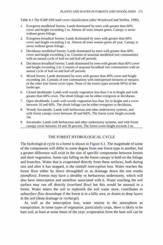
Table 6.1 The IGBP-DIS land cover classification (after Woodward and Steffen, 1996).
1. Evergreen needleleaf forests: Lands dominated by trees with greater than 60%cover and height exceeding 2 m. Almost all trees remain green. Canopy is neverwithout green foliage.
2. Evergreen broadleaf forests: Lands dominated by trees with greater than 60%cover and heighr exceeding 2 m. Almost all trees remain green all year. Canopy isnever without green foliage.
3. Deciduous needleleaf forests: Lands dominated by trees with greater than 60%cover and height exceeding 2 m. Consists of seasonal needleleaf tree communitieswith an annual cycle of leaf-on and leaf-off periods.
4. Deciduous broadleaf forests: Lands dominated by trees with greater than 60% coverand height exceeding 2 m. Consists of seasonal broadleaf tree communities with anannual cycle of leaf-on and leaf-off periods.
5. Mixed forests: Lands dominated by trees with greater than 60% cover and heightexceeding 2m. Consists of tree communities with interspersed mixtures or mosaicsof the other four forest cover types. None of the forest types exceeds 60%) of thelandscape.
6. Closed shrublands: Lands with woody vegetation less than 2 m in height and withgreater than 60% cover. The shrub foliage can be either evergreen or deciduous.
7. Open shrublands: Lands with woody vegetation less than 2m in height and a coverbetween 10 and 60%. The shrub foliage can be either evergreen or deciduous.
8. Woody Savannahs: Lands with herbaceous and other understorey systems, andwith forest canopy cover between 30 and 60(%. The forest cover height exceeds2m.
9. Savannahs: Lands with herbaceous and other understorey systems, and with forestcanopy cover between 10 and 30 percent. The forest cover height exceeds 2 m.
THE FOREST HYDROLOGICAL CYCLE
The hydrological cycle in a forest is shown in Figure 6.1. The magnitude of someof the components will differ to some degree from one forest type to another, buta greater difference will exist in the size of specific components between forestsand short vegetation. Some rain falling on the forest canopy is held on the foliageand branches. Water that is evaporated directly from these surfaces, both duringrain and after it has stopped, is the rainfall interception loss. Water reaches theforest floor either by direct throughfall or as drainage down the tree trunks(stemflow). Forests may have a shrubby or herbaceous understorey, which willalso have interception and stemflow associated with it. Water reaching the soilsurface may run off directly (overland flow) but this would be unusual in aforest. Water enters the soil to replenish the soil water store, contributes tosubsurface flow downslope if the forest is in a hilly area, or drains to deep layersin the soil (deep drainage or recharge).
As well as the interception loss, water returns to the atmosphere astranspiration. In some types of vegetation, particularly crops, there is likely to bebare soil, at least at some times of the year; evaporation from the bare soil can be
PLANTS AND WATER IN FORESTS AND WOODLANDS 171
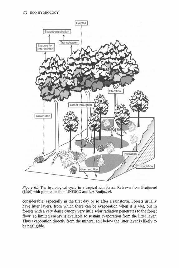
considerable, especially in the first day or so after a rainstorm. Forests usuallyhave litter layers, from which there can be evaporation when it is wet, but inforests with a very dense canopy very little solar radiation penetrates to the forestfloor, so limited energy is available to sustain evaporation from the litter layer.Thus evaporation directly from the mineral soil below the litter layer is likely tobe negligible.
Figure 6.1 The hydrological cycle in a tropical rain forest. Redrawn from Bruijnzeel(1990) with permission from UNESCO and L.A.Bruijnzeel.
172 ECO-HYDROLOGY
EVAPORATION FROM FORESTS
The traditional way to measure forest evaporation is to conduct catchmentexperiments to solve the water balance equation:
(6.1)where E is evaporation, P is precipitation, ∆S is the change in water storage ofthe soil or catchment, and R is runoff and drainage. Measuring E fromcatchments is often done over a twelve-month period, which allows theassumption that soil water conditions at the beginning and at the end will be thesame, so AS becomes negligible. These start and finish points are usually takenat some time when the soil is at or close to saturation. The calculation ofevaporation as the difference between precipitation and runoff assumes first thatboth can be accurately measured. Second, it is assumed that no liquid waterenters except as precipitation or leaves except through the stream-gauging device.
If different types of vegetation are to be compared by a catchment experimentit is required that the catchments be as similar as possible in all respects otherthan the vegetation. Important features of catchments that might influenceevaporation are slope and aspect, which influence exposure to radiation andwind, and soil and drainage conditions, which control the amount of wateravailable for evaporation. The difficulty of obtaining completely comparablecatchments with different vegetation can be tackled by comparing the twocatchments for a calibration period when they have the same vegetation. Thisapproach is usually improved by fitting regressions of runoff against climaticvariables for each catchment and testing the significance of before- and after-treatment regressions (Kovner and Evans, 1954).
Catchment experiments are the singular means for investigating effects ofcatchment management on the stream’s behaviour and its water quality, butunderstanding of evaporation and its controls can only proceed by using methodsthat separate the components of evaporation (interception and transpiration) andallow analysis of these processes in relation to seasonal and diurnal changes inenvironmental conditions. Measurements of interception and transpiration lossesfrom forests are usually made at scales smaller than that of the catchment; i.e. atthe leaf, tree or plot scale. Models would then be employed to exploit theinformation from these measurements at larger scales. The following sectionslook at the interception and transpiration processes in more detail.
INTERCEPTION
Measurement of rainfall interception
There is no reason why the evaporation of intercepted water cannot be measuredover short periods of as little as an hour or less, using the micrometeorologicalmethods of Bowen ratio or eddy covariance (see ‘Measurement of transpiration’,
PLANTS AND WATER IN FORESTS AND WOODLANDS 173
below). Practically, though, these methods are troublesome to use in wetconditions because raindrops will interfere with the correct operation of theinstruments or, because during and immediately after rainstorms, humiditydeficits of the atmosphere are small and gradients in the atmosphere would bedifficult to measure. Nevertheless, micrometeorological methods have been usedsuccessfully during and immediately after rainfall has ceased to investigate andunderstand processes controlling the rainfall evaporation process and todetermine short-term rates of evaporation from canopies under wet conditions(Stewart, 1977; Jarvis, 1993). More usually, interception loss from vegetation ismeasured as the difference between gross rainfall, either measured above theforest or in a nearby clearing, and net rainfall measured inside the forest. Thereare two main approaches to measuring net rainfall.
Plastic sheet rainfall collectors
Calder and Rosier (1976) describe a gauge that has been used successfully in anumber of forests in temperate and tropical regions. The gauge consists of a largeplastic sheet arranged on the forest floor as a series of roofs and troughs createdby joining rows of adjacent trees with ropes and laying the sheet over the ropeand back to ground level, with several such configurations repeated. At each treethe sheet is cut and sealed around the trunk with mastic compounds. The wholesheet slopes downwards in one direction and all the net rainfall (nodiscrimination is made between throughfall and stemflow) is led to a tippingbucket gauge connected to a data logger. If the gauge is to be left in place forextended periods of months or years, it will be necessary to provide sub-irrigation to prevent draughting and leaf fall of the trees in the gauge. A plasticsheet net rainfall gauge was used very effectively by Calder (1977) to provideestimates of rainfall interception and net rainfall inputs to a natural lysimeter inspruce forest in mid-Wales (see also ‘Measurement of transpiration’). Thisapproach was also used successfully in a tropical rain forest in Java (Calder etal., 1986). However, a similar approach proved unsuccessful in tropical rainforest in Amazonia (C.R.Lloyd, Institute of Hydrology, UK, personalcommunication) because an inordinately large gauge would have been necessaryto sample net rainfall adequately. In tropical rain forest, there are ‘drip points’where there can be a considerable concentration of throughfall. A plastic sheetgauge that is too small can conceivably sample one or several drip points, and itis possible to measure more net rainfall than gross rainfall. Alternatively, there isclearly a serious risk of under-sampling net rainfall.
Throughfall and stemflow gauges
Another common approach to measuring throughfall is to use fixed or movingrain gauges located randomly on the forest floor. Recording rain gauges can beused in the random positions, but this is likely to be prohibitively expensive. It is
174 ECO-HYDROLOGY
more usual to employ bottle gauges, which can be read manually at regularintervals or after rainstorms and then replaced or located in new randompositions. It will be necessary to measure stemflow separately, and this is usuallydone by attaching a guttering around the trunks of a number of trees andcollecting the stemflow in a container. Usually a number of trees are fitted withgauges, trees in the sample spanning the girth range of trees in the forest. Analternative to rain gauges on the forest floor are randomly located but fixedthroughfall troughs. There would also be a need for stemflow gauges asdescribed above.
A major challenge in interception studies is to achieve adequate sampling suchthat confidence limits on throughfall estimates are acceptably low. A plastic sheetnet rainfall gauge of around 100 m2 would be adequate in a young, denselystocked coniferous or broadleaf plantation, but there are other situations wherethe plastic sheet approach is likely to be unsuitable. In forests with widely spacedtrees the gauges would need to be excessively large to sample the variation inthroughfall. The problem of localised concentration of net rainfall in drip pointsin tropical rain forest has already been referred to. In tropical forests there islikely to be a similar problem for fixed trough gauges (Bruijnzeel and Wiersum,1987). When bottle gauges are used it is necessary to have a sufficiently largesample size; a further reduction in the error estimate of net rainfall will beachieved by randomly relocating gauges, preferably after individual rainstorms,but this may prove impractical in remote situations. The number of gauges foradequate sampling has been discussed for broadleaf woodlands by Czarnowskiand Olszewski (1970), for conifers by Kimmins (1973), and for tropical forest byLloyd and Marques Filho (1988). These last authors show that a better than 5percent error in the estimate of mean throughfall can be achieved with fortygauges with twenty random arrangements. Based on concerns about inadequatesampling, Bruijnzeel (1990) was sceptical about many reports of rainfallinterception losses for tropical forests.
Interception losses from forests
There are a considerable number of studies of rainfall interception in temperatebroadleaf and conifer forests. Figure 6.2 shows a representative portion of thedata that have come from studies in the UK. Because of the leafless nature ofbroadleaf forest canopies in winter, the interception fraction of gross rainfall isusually substantially less than for evergreen conifers in the same rainfall.
A feature of interception losses from temperate broadleaf forests (Figure 6.2)is that interception losses are far more variable at a given value of precipitationthan for conifers. A number of factors may contribute to this greater variability.Broadleaf forests in which interception studies have been carried out may havecontained a mixture of tree species and be of uneven age. Understoreys would bepresent in some forests but not in others. By contrast, the data for conifers would
PLANTS AND WATER IN FORESTS AND WOODLANDS 175
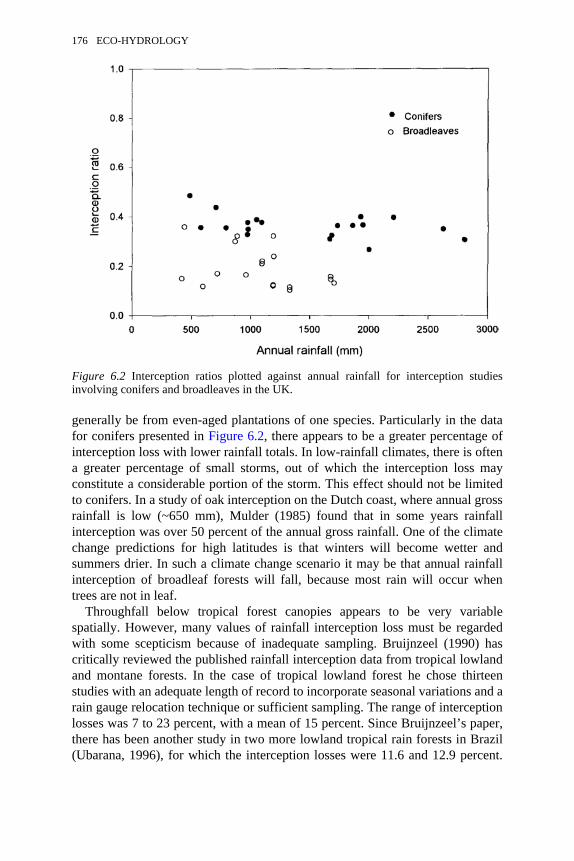
generally be from even-aged plantations of one species. Particularly in the datafor conifers presented in Figure 6.2, there appears to be a greater percentage ofinterception loss with lower rainfall totals. In low-rainfall climates, there is oftena greater percentage of small storms, out of which the interception loss mayconstitute a considerable portion of the storm. This effect should not be limitedto conifers. In a study of oak interception on the Dutch coast, where annual grossrainfall is low (~650 mm), Mulder (1985) found that in some years rainfallinterception was over 50 percent of the annual gross rainfall. One of the climatechange predictions for high latitudes is that winters will become wetter andsummers drier. In such a climate change scenario it may be that annual rainfallinterception of broadleaf forests will fall, because most rain will occur whentrees are not in leaf.
Throughfall below tropical forest canopies appears to be very variablespatially. However, many values of rainfall interception loss must be regardedwith some scepticism because of inadequate sampling. Bruijnzeel (1990) hascritically reviewed the published rainfall interception data from tropical lowlandand montane forests. In the case of tropical lowland forest he chose thirteenstudies with an adequate length of record to incorporate seasonal variations and arain gauge relocation technique or sufficient sampling. The range of interceptionlosses was 7 to 23 percent, with a mean of 15 percent. Since Bruijnzeel’s paper,there has been another study in two more lowland tropical rain forests in Brazil(Ubarana, 1996), for which the interception losses were 11.6 and 12.9 percent.
Figure 6.2 Interception ratios plotted against annual rainfall for interception studiesinvolving conifers and broadleaves in the UK.
176 ECO-HYDROLOGY
For six montane forests thought by Bruijnzeel (1990) to have adequate sampling,the range of interception loss was from 14 to 25 percent, with a mean of 19percent. The higher values for the montane tropical forests are thought to be dueto lower rainfall intensities prevailing on tropical mountains.
Thus the fraction of gross rainfall lost as interception is lower for tropicalforests than for temperate forests. The reasons for this are explored in‘Comparison of temperate coniferous forest and tropical rainforest’, below.
Modelling rainfall interception
Up to the 1960s, most results from interception were examined in the form ofempirical regression equations relating interception loss to gross precipitation. Inthe UK, there was increased interest in the interception process following thethen controversial results of Law (1956; 1958), which suggested that a sitkaspruce forest used nearly 300 mm more water per year than adjacent grassland.In an attempt to repeat and explain Law’s results, Rutter and others developed aphysically based model of interception loss from forests (Rutter et al., 1971;1975). The Rutter model calculates a running water balance for the canopy andtrunks of the forest using input data of hourly rainfall and the meteorologicalparameters necessary to estimate evaporation. It computes the rates ofevaporation of intercepted water, and also the amount of water reaching theground either directly or via throughfall and stemflow. The Rutter model hasbeen successfully tested using independent data (e.g. Calder, 1977, and Gash andMorton, 1978) but has the disadvantage that it requires hourly rainfall andweather data to be used in forecasting mode.
Gash (1979) described an analytical model that linked Rutter’s approach withearlier regression approaches. The Gash model is a storm-based approach thatrequires a knowledge of the capacity for vegetation to store water and theaverage rates of evaporation and precipitation during rainfall. It can be used topredict rainfall interception given basic daily rainfall data available from moststandard meteorological stations (Lloyd and Marques Filho, 1988). The modelhas been used successfully in a number of forests such as coniferous forests inthe UK (Gash et al., 1980), evergreen mixed forest in New Zealand (Pearce andRowe, 1981), oak forest in the Netherlands (Dolman, 1987), tropical forestplantations (Bruijnzeel and Wiersum, 1987), and rain forest in Amazonia (Lloydet al., 1988) and West Africa (Hutjes et al., 1990).
An alternative approach to modelling rainfall interception from forest canopieshas been the use of the so-called stochastic model (Calder, 1986). In this model,the wetting of the canopy is related to probabilities of raindrops striking thecanopy elements. The model also predicts that, for the same total rainfallamounts, maximum water storage on the canopy will be reached more slowlywith larger raindrops. Calder’s model has been used successfully for tropical rainforest in Java (Calder et al., 1986) and tropical rain forest and plantations in SriLanka and India (Calder, 1996; Calder et al., 1996; Hall et al., 1996).
PLANTS AND WATER IN FORESTS AND WOODLANDS 177
Increasingly, agroforestry systems involving trees and crops growing incombination are being used to enhance productivity on marginal lands indeveloping countries. It is important to estimate rainfall interception as this is animportant water loss from the agroforestry system. The Gash model wasunsuccessful in modelling sparse forest interception loss (Teklehaimanot et al.,1991). Gash et al. (1995) reformulated the original Gash model usingevaporation per unit of canopy rather than per unit of ground area. The newmodel performed well in predicting rainfall interception for Les Landes forest,France (ibid.) and eucalyptus plantations in Portugal (Valente et al., 1997).These two examples are open forest plantations, but it is likely that the modelwill probably be very valuable for predicting interception losses from nativevegetation where tree cover is sparse, e.g. woody savannahs and agroforestrysystems.
TRANSPIRATION
Measurement of transpiration
Because there are a wide range of questions relating to transpiration from forests,a wide range of techniques have been used to measure the process. Whichtechnique should be used depends on the temporal and spatial scale over whichestimates are needed.
Soil water depletion
Studies of rates of soil water depletion are usually used to estimate transpirationover timescales of at least a few days, and they cannot distinguish water taken upby different species when they are growing in close proximity. Sufficientmeasurements of soil water content need to be made to account for spatialvariation in water storage. In addition, the amount of drainage needs to bemeasured, or it must be insignificant. Provided drainage from and recharge to thesoil is quantified or insignificant, changes in soil water storage allow evaporationto be calculated when rainfall is absent or measured separately. Soil moisturedepletion techniques require repeated in situ measurements of soil water content,which may be with a neutron probe (Bell, 1987; Greacen, 1981), capacitanceprobe (Bell et al., 1987; Dean et al., 1987), the impedance ‘ThetaProbe’technique (Gaskin and Miller, 1996), or by using time domain reflectometry(Topp et al., 1980; 1984).
178 ECO-HYDROLOGY
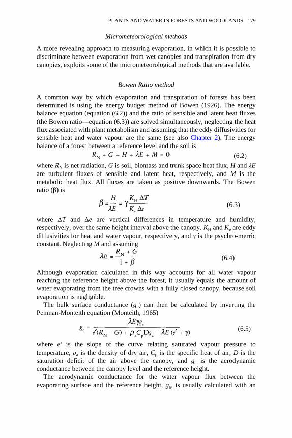
Micrometeorological methods
A more revealing approach to measuring evaporation, in which it is possible todiscriminate between evaporation from wet canopies and transpiration from drycanopies, exploits some of the micrometeorological methods that are available.
Bowen Ratio method
A common way by which evaporation and transpiration of forests has beendetermined is using the energy budget method of Bowen (1926). The energybalance equation (equation (6.2)) and the ratio of sensible and latent heat fluxes(the Bowen ratio—equation (6.3)) are solved simultaneously, neglecting the heatflux associated with plant metabolism and assuming that the eddy diffusivities forsensible heat and water vapour are the same (see also Chapter 2). The energybalance of a forest between a reference level and the soil is
(6.2)where RN is net radiation, G is soil, biomass and trunk space heat flux, H and λEare turbulent fluxes of sensible and latent heat, respectively, and M is themetabolic heat flux. All fluxes are taken as positive downwards. The Bowenratio (β) is
(6.3)
where ∆T and ∆e are vertical differences in temperature and humidity,respectively, over the same height interval above the canopy. KH and Ke are eddydiffusivities for heat and water vapour, respectively, and γ is the psychro-merricconstant. Neglecting M and assuming
(6.4)
Although evaporation calculated in this way accounts for all water vapourreaching the reference height above the forest, it usually equals the amount ofwater evaporating from the tree crowns with a fully closed canopy, because soilevaporation is negligible.
The bulk surface conductance (gc) can then be calculated by inverting thePenman-Monteith equation (Monteith, 1965)
(6.5)
where e′ is the slope of the curve relating saturated vapour pressure totemperature, ρa is the density of dry air, Cp is the specific heat of air, D is thesaturation deficit of the air above the canopy, and ga is the aerodynamicconductance between the canopy level and the reference height.
The aerodynamic conductance for the water vapour flux between theevaporating surface and the reference height, ga, is usually calculated with an
PLANTS AND WATER IN FORESTS AND WOODLANDS 179

equation similar to the one below, with z0 and d being assumed proportional tothe stand height, b, and arbitrarily chosen as d=0.8h and z0=0.lh
(6.6)
where z is the reference height of the energy balance measurements, z0 is thesurface roughness length, d is the zero plane displacement, k is von Karman’sconstant and u(z) is the windspeed at height z.
There are some practical difficulties associated with measuring forestevaporation with the energy budget—Bowen ratio—method. There is, of course,a need for a tower to mount instruments some metres above the tallestsurrounding trees. The main difficulty, though, is the requirement to measuregradients of temperature and humidity (∆T and ∆e) in the air above the forest.Because of the particularly good mixing of the air above forests, these gradientsare often only a few tenths of a °C, substantially smaller than those observedabove short vegetation. The measurements of dry- and wet-bulb temperatures toresolve ∆T and ∆e required to calculate the Bowen ratio, β, are usually madewith thermometers calibrated to one-hundreth of a degree, but systematicdifferences between sensors may be large enough to partly obscure gradients. Anapproach that has been adopted to resolve gradients that are close to theinstrumental errors has been to devise electronically controlled, mechanicaldevices (usually trackways or rotating booms) that systematically interchangethermometers between upper and lower levels several times in an hour. Anexample of such a device has been described by McNeil and Shuttleworth(1975).
Eddy correlation method
Within the turbulent boundary layer generated near the ground by the interactionof wind with surface irregularities, the transfer of water vapour and otheratmospheric entities occurs by the process of turbulent diffusion. Although themean wind speed at each level near the surface is parallel to the ground, theinstantaneous air movement at any point can assume any direction, and, ingeneral, there will be a component of wind moving towards and a componentmoving away from the forest surface, with a mean value of zero but with a finitestandard deviation. It is this fluctuating component of wind that transports heatand water vapour away from or to the surface. Evaporation can be measured bymaking simultaneous measurements of both fluctuations in the wind componentnormal to the forest surface and fluctuations in the humidity of the air at thesame point. The algebraic product of these variables is the instantaneous vapourflux, which can be either positive or negative at any instant (depending on thestatistical nature of the turbulent transfer process), but which has a finite meanvalue, the net evaporation loss from the surface, found by integrating the
180 ECO-HYDROLOGY
instantaneous flux. A comprehensive account of the eddy correlation approachcan be found in Shuttleworth (1992).
The sensors to measure wind speed and humidity have very rapid responsesand must be located close to each other to measure the same parcel of air. Eddycorrelation is now the favoured means of measuring evaporation directly fromvegetation. This preference has been further enhanced in the last few yearsbecause approaches have evolved that have enabled measurements ofevaporation and CO2 exchange to be combined in a single piece of equipment.The CO2 measurement is made by ducting small air samples, from where windspeed and humidity are measured, into a fast-response infrared gas analyser(Moncrieff et al., 1997).
Until recently, a perceived limitation of micrometeorological techniques wastheir inability to measure fluxes from components of the forest such as the litterlayer or the understorey. A number of recent studies have attempted to measurewater vapour fluxes within forests using an eddy correlation device additional toone operating above the forest (e.g. Black et al., 1996) and increasingly, as withabove-canopy measurements, measurements of water vapour fluxes are beingmade in conjunction with those of carbon dioxide. There is a specific interest inCO2 flux measurements, from which net carbon exchange of forests or theircomponents can be estimated, but additionally, with information about vapourfluxes from transpiration, water use efficiency estimates can be made.
Lysimeters
A lysimeter is a device in which a volume of soil with associated vegetation isisolated hydrologically from the surrounding soil. Drainage is measured or iszero and, in the case of lysimeters that are weighed, changes in water storage aredetermined by weight difference. The application of weighing lysimeters tostudies in mature or semi-mature forests has been very limited. A single largeDouglas fir tree was installed in a weighing lysimeter by Fritschen et al. (1973),and Reyenga et al. (1988) installed a lysimeter in a regenerating eucalyptus forestin New South Wales, Australia. Large potted trees capable of being weighed (upto 500 kg) have proved useful for calibrating other techniques such as isotopetracers (e.g. Dugas et al., 1993). Another form of lysimeter is the drainagelysimeter, which has been used very commonly in short crops but rarely inforests. Calder (1976) described a drainage lysimeter constructed in a Norwayspruce plantation in mid-Wales, UK. The base of the lysimeter was sealednaturally by impermeable clay. Data from the lysimeter associated with nearbynet rainfall measurements enabled calculation of three separate years oftranspiration loss (Calder, 1977).
PLANTS AND WATER IN FORESTS AND WOODLANDS 181
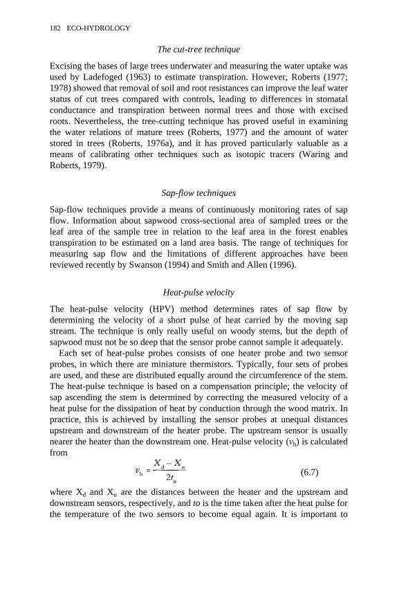
The cut-tree technique
Excising the bases of large trees underwater and measuring the water uptake wasused by Ladefoged (1963) to estimate transpiration. However, Roberts (1977;1978) showed that removal of soil and root resistances can improve the leaf waterstatus of cut trees compared with controls, leading to differences in stomatalconductance and transpiration between normal trees and those with excisedroots. Nevertheless, the tree-cutting technique has proved useful in examiningthe water relations of mature trees (Roberts, 1977) and the amount of waterstored in trees (Roberts, 1976a), and it has proved particularly valuable as ameans of calibrating other techniques such as isotopic tracers (Waring andRoberts, 1979).
Sap-flow techniques
Sap-flow techniques provide a means of continuously monitoring rates of sapflow. Information about sapwood cross-sectional area of sampled trees or theleaf area of the sample tree in relation to the leaf area in the forest enablestranspiration to be estimated on a land area basis. The range of techniques formeasuring sap flow and the limitations of different approaches have beenreviewed recently by Swanson (1994) and Smith and Allen (1996).
Heat-pulse velocity
The heat-pulse velocity (HPV) method determines rates of sap flow bydetermining the velocity of a short pulse of heat carried by the moving sapstream. The technique is only really useful on woody stems, but the depth ofsapwood must not be so deep that the sensor probe cannot sample it adequately.
Each set of heat-pulse probes consists of one heater probe and two sensorprobes, in which there are miniature thermistors. Typically, four sets of probesare used, and these are distributed equally around the circumference of the stem.The heat-pulse technique is based on a compensation principle; the velocity ofsap ascending the stem is determined by correcting the measured velocity of aheat pulse for the dissipation of heat by conduction through the wood matrix. Inpractice, this is achieved by installing the sensor probes at unequal distancesupstream and downstream of the heater probe. The upstream sensor is usuallynearer the heater than the downstream one. Heat-pulse velocity (νh) is calculatedfrom
(6.7)
where Xd and Xu are the distances between the heater and the upstream anddownstream sensors, respectively, and to is the time taken after the heat pulse forthe temperature of the two sensors to become equal again. It is important to
182 ECO-HYDROLOGY
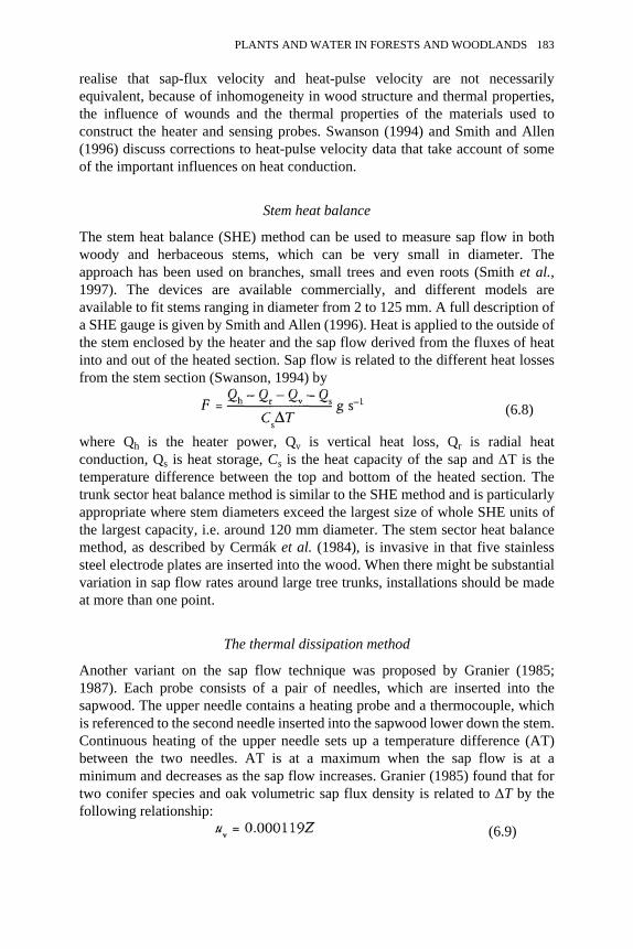
realise that sap-flux velocity and heat-pulse velocity are not necessarilyequivalent, because of inhomogeneity in wood structure and thermal properties,the influence of wounds and the thermal properties of the materials used toconstruct the heater and sensing probes. Swanson (1994) and Smith and Allen(1996) discuss corrections to heat-pulse velocity data that take account of someof the important influences on heat conduction.
Stem heat balance
The stem heat balance (SHE) method can be used to measure sap flow in bothwoody and herbaceous stems, which can be very small in diameter. Theapproach has been used on branches, small trees and even roots (Smith et al.,1997). The devices are available commercially, and different models areavailable to fit stems ranging in diameter from 2 to 125 mm. A full description ofa SHE gauge is given by Smith and Allen (1996). Heat is applied to the outside ofthe stem enclosed by the heater and the sap flow derived from the fluxes of heatinto and out of the heated section. Sap flow is related to the different heat lossesfrom the stem section (Swanson, 1994) by
(6.8)
where Qh is the heater power, Qν is vertical heat loss, Qr is radial heatconduction, Qs is heat storage, Cs is the heat capacity of the sap and ∆T is thetemperature difference between the top and bottom of the heated section. Thetrunk sector heat balance method is similar to the SHE method and is particularlyappropriate where stem diameters exceed the largest size of whole SHE units ofthe largest capacity, i.e. around 120 mm diameter. The stem sector heat balancemethod, as described by Cermák et al. (1984), is invasive in that five stainlesssteel electrode plates are inserted into the wood. When there might be substantialvariation in sap flow rates around large tree trunks, installations should be madeat more than one point.
The thermal dissipation method
Another variant on the sap flow technique was proposed by Granier (1985;1987). Each probe consists of a pair of needles, which are inserted into thesapwood. The upper needle contains a heating probe and a thermocouple, whichis referenced to the second needle inserted into the sapwood lower down the stem.Continuous heating of the upper needle sets up a temperature difference (AT)between the two needles. AT is at a maximum when the sap flow is at aminimum and decreases as the sap flow increases. Granier (1985) found that fortwo conifer species and oak volumetric sap flux density is related to ∆T by thefollowing relationship:
(6.9)
PLANTS AND WATER IN FORESTS AND WOODLANDS 183
where
(6.10)
when ∆T0 is the value of ∆T when there is no sap flow. The mass sap flow rate isthen
(6.11)where ρs is the sap density and Asw is the sapwood cross-sectional area. Granier etal. (1990) suggest that the parameters in equation (6.9) are not dependent onwood properties or tree species and that the technique may possibly be usedwithout calibration. However, this possibility needs testing for a wider range ofspecies than has been achieved so far. This is important, because Granier-typegauges are available commercially at reasonable cost and are likely to becomewidely used in the future because they are simple to install, the calculations toderive sap flow are straightforward, and the gauges have relatively simple data-logging requirements.
Parameters and infrared gas analysers
A range of porometers and portable infrared gas analysers (IRGAs) with leafchambers are commercially available. Porometers enable measurements ofstomatal conductance, gs, of individual leaves to be measured in situ. An IRGAcan also be used to determine CO2 exchange from the leaf as well as gs.Additional useful information that can be acquired or calculated are leaftranspiration rates, leaf temperatures and internal CO2 concentration of theleaves. gs determined with porometers and IRGAs gives the smallest temporaland spatial scale of information and provides considerable insight into theenvironmental and internal controls of gs and hence transpiration.
gs measured with porometers and IRGAs has also been used to estimatetranspiration from plant canopies. This involves multiplying gs by the leaf areaindex to produce a surface or canopy conductance (gc). gc is used with a canopyboundary layer conductance, ga (Grace, 1983), to estimate transpiration using thePenman-Monteith equation (Monteith, 1965). It is possible to follow thisprocedure in very complex canopies. An extreme case would be the tropical rainforest studied by Roberts et al. (1993). However, such an enterprise requirescanopy access, and considerable effort has to be dedicated to sampling thecanopy. Additionally, information about the leaf area index of the vegetationmust be available, and in a complex canopy the vertical distribution of the leafarea may need to be known. Nevertheless, particularly with IRGAs, the availabletechnology has become very sophisticated, so that environmental conditions suchas light, vapour pressure deficit, temperature and CO2 concentration can bemanipulated in the IRGA and the response of the leaf determined.
184 ECO-HYDROLOGY
Radioactive and stable isotope tracers
A number of tracers have been used to measure transpiration from branches andindividual trees. These values can then be scaled up to give stand transpiration.Waring and Roberts (1979) used P32 and tritium to measure the transpiration ofScots pine trees. The isotopes were injected at the base of the tree and measuredover the next few days as the tracers moved up the tree. Calder et al. (1992)described an approach using deuterium oxide (D2O), which was injected intoeucalyptus trees in plantations. Transpired water was collected in polythene bagstied onto selected branches. From the information of the D2O injected (M) andthe concentration in the transpirate produced over a known time interval (Cdt),transpiration (F) can be calculated
(6.12)The tracing techniques are simple to apply, and useful results are produced thatagree well with other methods. However, there are obvious safety constraints inusing radioactive isotopes and, where transpirate needs to be collected, there isstill a need for canopy access. The time resolution for tracing techniques isrelatively low as well. Transpiration values can only be resolved over as little asa few days. It is, therefore, difficult to use the techniques to understand theinfluence of short-term environmental fluctuations on transpiration.
Transpiration from forests
Table 6.1 lists a range of vegetation types that have woody plants as a keycomponent of the vegetation. Unfortunately, there are not, as yet, comprehensivehydrological studies for all the classes in the table. For most of the classes thereis some physiological information, with details of processes at the leaf level anddata relating to biomass and leaf area. However, there are many gaps preventinga fuller understanding of the hydrological processes. It is only recently, largelybecause of interest in carbon sinks, that intensive studies into the boreal foresthave been initiated, and a full output from the BOREAS project (Sellers et al.,1995) should provide considerably more insight than is currently available. Inthis section, information from a selection of woody vegetation types is examinedand attention drawn to the key features of hydrological behaviour. The threetypes selected arguably represent three quite separate points on the spectrum ofannual rainfall supplied to the forest or woodland type.
Temperate forests
These forests comprise both conifers and broadleaves, and, of all forests, thereare most data for this type because of the many detailed studies in temperateregions aimed at obtaining information about forest ecology, hydrology andbiogeochemistry. Studies have been concentrated in Western Europe and NorthAmerica.
PLANTS AND WATER IN FORESTS AND WOODLANDS 185
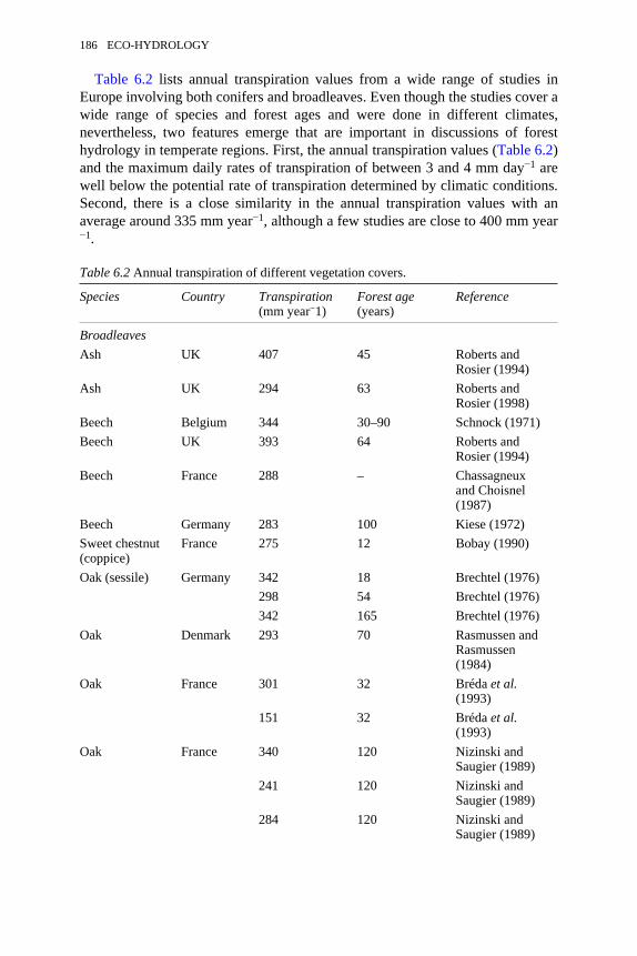
Table 6.2 lists annual transpiration values from a wide range of studies inEurope involving both conifers and broadleaves. Even though the studies cover awide range of species and forest ages and were done in different climates,nevertheless, two features emerge that are important in discussions of foresthydrology in temperate regions. First, the annual transpiration values (Table 6.2)and the maximum daily rates of transpiration of between 3 and 4 mm day−1 arewell below the potential rate of transpiration determined by climatic conditions.Second, there is a close similarity in the annual transpiration values with anaverage around 335 mm year−1, although a few studies are close to 400 mm year−1.
Table 6.2 Annual transpiration of different vegetation covers.
Species Country Transpiration(mm year−1)
Forest age(years)
Reference
BroadleavesAsh UK 407 45 Roberts and
Rosier (1994)Ash UK 294 63 Roberts and
Rosier (1998)Beech Belgium 344 30–90 Schnock (1971)Beech UK 393 64 Roberts and
Rosier (1994)Beech France 288 – Chassagneux
and Choisnel(1987)
Beech Germany 283 100 Kiese (1972)Sweet chestnut(coppice)
France 275 12 Bobay (1990)
Oak (sessile) Germany 342 18 Brechtel (1976)298 54 Brechtel (1976)342 165 Brechtel (1976)
Oak Denmark 293 70 Rasmussen andRasmussen(1984)
Oak France 301 32 Bréda et al.(1993)
151 32 Bréda et al.(1993)
Oak France 340 120 Nizinski andSaugier (1989)
241 120 Nizinski andSaugier (1989)
284 120 Nizinski andSaugier (1989)
186 ECO-HYDROLOGY
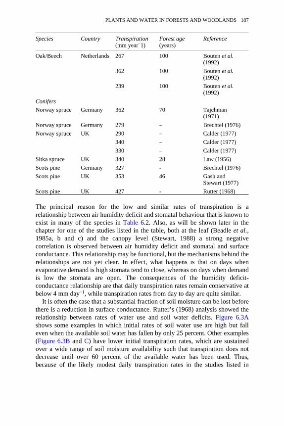
Species Country Transpiration(mm year−1)
Forest age(years)
Reference
Oak/Beech Netherlands 267 100 Bouten et al.(1992)
362 100 Bouten et al.(1992)
239 100 Bouten et al.(1992)
ConifersNorway spruce Germany 362 70 Tajchman
(1971)Norway spruce Germany 279 – Brechtel (1976)Norway spruce UK 290 – Calder (1977)
340 – Calder (1977)330 – Calder (1977)
Sitka spruce UK 340 28 Law (1956)Scots pine Germany 327 - Brechtel (1976)Scots pine UK 353 46 Gash and
Stewart (1977)Scots pine UK 427 - Rutter (1968)
The principal reason for the low and similar rates of transpiration is arelationship between air humidity deficit and stomatal behaviour that is known toexist in many of the species in Table 6.2. Also, as will be shown later in thechapter for one of the studies listed in the table, both at the leaf (Beadle et al.,1985a, b and c) and the canopy level (Stewart, 1988) a strong negativecorrelation is observed between air humidity deficit and stomatal and surfaceconductance. This relationship may be functional, but the mechanisms behind therelationships are not yet clear. In effect, what happens is that on days whenevaporative demand is high stomata tend to close, whereas on days when demandis low the stomata are open. The consequences of the humidity deficit-conductance relationship are that daily transpiration rates remain conservative atbelow 4 mm day−1, while transpiration rates from day to day are quite similar.
It is often the case that a substantial fraction of soil moisture can be lost beforethere is a reduction in surface conductance. Rutter’s (1968) analysis showed therelationship between rates of water use and soil water deficits. Figure 6.3Ashows some examples in which initial rates of soil water use are high but falleven when the available soil water has fallen by only 25 percent. Other examples(Figure 6.3B and C) have lower initial transpiration rates, which are sustainedover a wide range of soil moisture availability such that transpiration does notdecrease until over 60 percent of the available water has been used. Thus,because of the likely modest daily transpiration rates in the studies listed in
PLANTS AND WATER IN FORESTS AND WOODLANDS 187
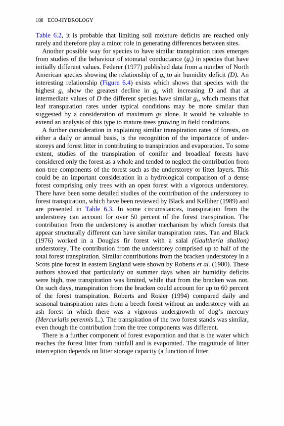
Table 6.2, it is probable that limiting soil moisture deficits are reached onlyrarely and therefore play a minor role in generating differences between sites.
Another possible way for species to have similar transpiration rates emergesfrom studies of the behaviour of stomatal conductance (gs) in species that haveinitially different values. Federer (1977) published data from a number of NorthAmerican species showing the relationship of gs to air humidity deficit (D). Aninteresting relationship (Figure 6.4) exists which shows that species with thehighest gs show the greatest decline in gs with increasing D and that atintermediate values of D the different species have similar gs, which means thatleaf transpiration rates under typical conditions may be more similar thansuggested by a consideration of maximum gs alone. It would be valuable toextend an analysis of this type to mature trees growing in field conditions.
A further consideration in explaining similar transpiration rates of forests, oneither a daily or annual basis, is the recognition of the importance of under-storeys and forest litter in contributing to transpiration and evaporation. To someextent, studies of the transpiration of conifer and broadleaf forests haveconsidered only the forest as a whole and tended to neglect the contribution fromnon-tree components of the forest such as the understorey or litter layers. Thiscould be an important consideration in a hydrological comparison of a denseforest comprising only trees with an open forest with a vigorous understorey.There have been some detailed studies of the contribution of the understorey toforest transpiration, which have been reviewed by Black and Kelliher (1989) andare presented in Table 6.3. In some circumstances, transpiration from theunderstorey can account for over 50 percent of the forest transpiration. Thecontribution from the understorey is another mechanism by which forests thatappear structurally different can have similar transpiration rates. Tan and Black(1976) worked in a Douglas fir forest with a salal (Gaultheria shallon)understorey. The contribution from the understorey comprised up to half of thetotal forest transpiration. Similar contributions from the bracken understorey in aScots pine forest in eastern England were shown by Roberts et al. (1980). Theseauthors showed that particularly on summer days when air humidity deficitswere high, tree transpiration was limited, while that from the bracken was not.On such days, transpiration from the bracken could account for up to 60 percentof the forest transpiration. Roberts and Rosier (1994) compared daily andseasonal transpiration rates from a beech forest without an understorey with anash forest in which there was a vigorous undergrowth of dog’s mercury(Mercurialis perennis L.). The transpiration of the two forest stands was similar,even though the contribution from the tree components was different.
There is a further component of forest evaporation and that is the water whichreaches the forest litter from rainfall and is evaporated. The magnitude of litterinterception depends on litter storage capacity (a function of litter
188 ECO-HYDROLOGY
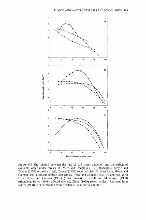
Figure 6.3 The relation between the rate of soil water depletion and the deficit ofavailable water under forests. A: Metz and Douglass (1959) (triangles); Moyle andZahner (1954) (closed circles); Zahner (1955) (open circles). B: Bass Lake, Rowe andColman (1951) (closed circles); San Dimas, Rowe and Colman (1951) (triangles); NorthFork, Rowe and Colman (1951) (open circles). C: Croft and Monninger (1953)(triangles); Rowe (1948) (closed circles); Zinke (1959) (open circles). Redrawn fromRutter (1968) with permission from Academic Press and A.J.Rutter.
PLANTS AND WATER IN FORESTS AND WOODLANDS 189
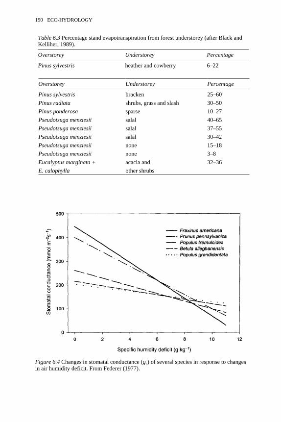
Figure 6.4 Changes in stomatal conductance (gs) of several species in response to changesin air humidity deficit. From Federer (1977).
190 ECO-HYDROLOGY
Overstorey Understorey Percentage
Pinus sylvestris bracken 25–60Pinus radiata shrubs, grass and slash 30–50Pinus ponderosa sparse 10–27Pseudotsuga menziesii salal 40–65Pseudotsuga menziesii salal 37–55Pseudotsuga menziesii salal 30–42Pseudotsuga menziesii none 15–18Pseudotsuga menziesii none 3–8Eucalyptus marginata + acacia and 32–36E. calophylla other shrubs
Table 6.3 Percentage stand evapotranspiration from forest understorey (after Black andKelliher, 1989).
Overstorey Understorey Percentage
Pinus sylvestris heather and cowberry 6–22
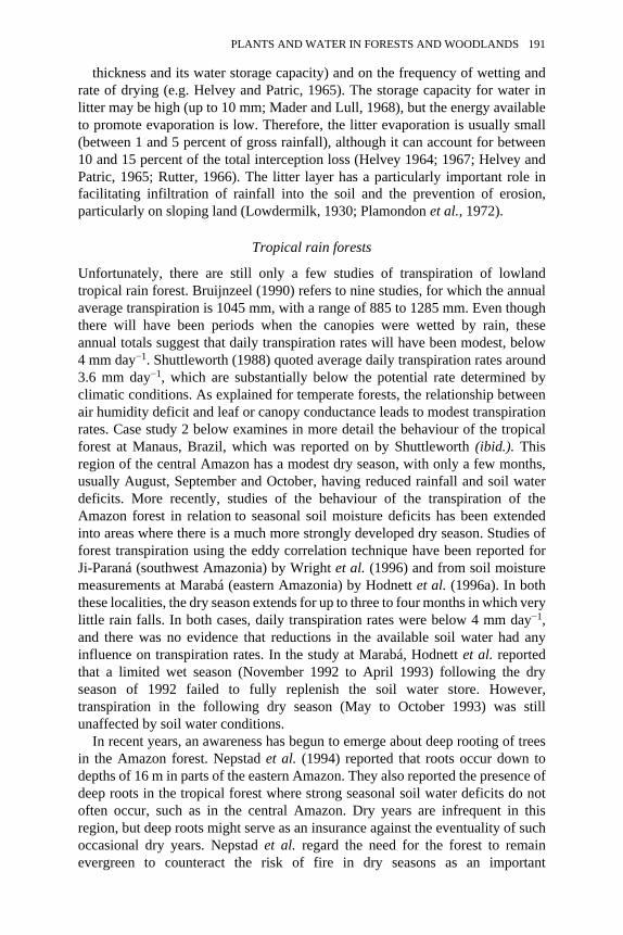
facilitating infiltration of rainfall into the soil and the prevention of erosion,particularly on sloping land (Lowdermilk, 1930; Plamondon et al., 1972).
Tropical rain forests
Unfortunately, there are still only a few studies of transpiration of lowlandtropical rain forest. Bruijnzeel (1990) refers to nine studies, for which the annualaverage transpiration is 1045 mm, with a range of 885 to 1285 mm. Even thoughthere will have been periods when the canopies were wetted by rain, theseannual totals suggest that daily transpiration rates will have been modest, below4 mm day−1. Shuttleworth (1988) quoted average daily transpiration rates around3.6 mm day−1, which are substantially below the potential rate determined byclimatic conditions. As explained for temperate forests, the relationship betweenair humidity deficit and leaf or canopy conductance leads to modest transpirationrates. Case study 2 below examines in more detail the behaviour of the tropicalforest at Manaus, Brazil, which was reported on by Shuttleworth (ibid.). Thisregion of the central Amazon has a modest dry season, with only a few months,usually August, September and October, having reduced rainfall and soil waterdeficits. More recently, studies of the behaviour of the transpiration of theAmazon forest in relation to seasonal soil moisture deficits has been extendedinto areas where there is a much more strongly developed dry season. Studies offorest transpiration using the eddy correlation technique have been reported forJi-Paraná (southwest Amazonia) by Wright et al. (1996) and from soil moisturemeasurements at Marabá (eastern Amazonia) by Hodnett et al. (1996a). In boththese localities, the dry season extends for up to three to four months in which verylittle rain falls. In both cases, daily transpiration rates were below 4 mm day−1,and there was no evidence that reductions in the available soil water had anyinfluence on transpiration rates. In the study at Marabá, Hodnett et al. reportedthat a limited wet season (November 1992 to April 1993) following the dryseason of 1992 failed to fully replenish the soil water store. However,transpiration in the following dry season (May to October 1993) was stillunaffected by soil water conditions.
In recent years, an awareness has begun to emerge about deep rooting of treesin the Amazon forest. Nepstad et al. (1994) reported that roots occur down todepths of 16 m in parts of the eastern Amazon. They also reported the presence ofdeep roots in the tropical forest where strong seasonal soil water deficits do notoften occur, such as in the central Amazon. Dry years are infrequent in thisregion, but deep roots might serve as an insurance against the eventuality of suchoccasional dry years. Nepstad et al. regard the need for the forest to remainevergreen to counteract the risk of fire in dry seasons as an important
PLANTS AND WATER IN FORESTS AND WOODLANDS 191
thickness and its water storage capacity) and on the frequency of wetting andrate of drying (e.g. Helvey and Patric, 1965). The storage capacity for water inlitter may be high (up to 10 mm; Mader and Lull, 1968), but the energy availableto promote evaporation is low. Therefore, the litter evaporation is usually small(between 1 and 5 percent of gross rainfall), although it can account for between10 and 15 percent of the total interception loss (Helvey 1964; 1967; Helvey andPatric, 1965; Rutter, 1966). The litter layer has a particularly important role in

need to extract water from below 2 m in the soil to sustain transpiration rates atthe average of 3.6 mm day−1 (Shuttleworth, 1988).
There are, however, a number of examples for which annual transpiration ofseasonally dry tropical forests is substantially less than the figures quoted above(~1000 mm year−1) for lowland tropical rain forests. Studies by Dietrich et al.(1982) in Panama and by Gilmour (1977) and Bonell and Gilmour (1978) inQueensland, Australia, indicated values below 500 mm year−1. Bruijnzeel (1990)quotes figures of between 510 and 810 mm year−1 for montane tropical forests.Bruijnzeel and Proctor (1995) collected what little information there is ontranspiration rates of montane tropical rain forests. Annual and daily rates arevery low, presumably because of the low radiation conditions in the predominantcloud cover. There is a need for more comprehensive studies of transpiration aswell as other hydrological processes in montane tropical rain forests.
Semi-arid woodlands
In comparison with woody vegetation in other regions, there is a paucity ofinformation about annual, seasonal and daily transpiration from woodlands in thesemi-arid tropics. The ecological functioning of such woodlands and fallowsavannahs has particular importance in the Sahel, where they provide fuel andfodder for local people, and their animals. Grazing, particularly by sheep andgoats, and fuelwood collection prevent the regeneration of natural woodland inareas where bushland has been allowed to regrow as fallow after cropping. Acombination of drought, grazing and fuelwood exploitation can impose suchpressures on the vegetation that desertification is started, the degraded vegetationhaving large areas of bare soil, which can be susceptible to erosion. Charney(1975) outlined a mechanism by which the higher albedo of bare soil can lead toatmospheric processes resulting in lower rainfall. The hydrological and surfaceenergy balance processes of semi-arid tropical regions are of considerableimportance.
There are at least two problems in interpreting what hydrological data thereare for semi-arid woodlands. Usually only total evaporation data are available,with no distinctions being made between evaporation of intercepted water andtranspiration. Second, because there are often substantial areas of bare soil,evaporation from the soil is often included in the transpiration term.Nevertheless, some generalisations can be made from the recent studies that havebeen made. Culf et al. (1993) showed that evaporation of striped woodland ‘tigerbush’ in Niger, West Africa, accounted for almost all the annual rainfall. Duringthe wet season, evaporation rates were above 4 mm day−1 but fell to around 1.5mm day−1 in the dry season. Soil evaporation accounted for about 25 percent oftotal evaporation. Measurements of evaporation from fallow savannah by Gashet al. (1991) showed similar values of evaporation in the wet and dry season tothose reported for the natural vegetation by Culf et al. Similar results were alsoobtained for thorn scrub (Acacia tortilis and Balanites aegyptiaca) in northern
192 ECO-HYDROLOGY
in the central Amazon and use of a simple soil water balance model, Hodnett et al.(1996b) showed that, on average, once every nine years the tropical forest would
consideration. From a study of twenty-seven years of rainfall record for Manaus
Senegal by Nizinski et al. (1994). Maximum evaporation rates (probablyincluding some interception losses) in the wet season were above 5 mm day−1 forAcacia and around 4 mm day−1 for Balanites. These rates fell to 0.93 and 0.46mm day−1, respectively, in the hot dry season. As in the study by Culf et al.,Nizinski et al. suggest that very little residual water is left in the profile at theend of the dry season, especially below Acacia. Interception losses were around12 percent of gross rainfall.
The past decade has seen considerable research activity in the Sahel. One ofthe key research aims has been to examine the interaction of land-surfaceprocesses and climatology. In this context, a number of studies have determinedenergy and water balances of pristine Sahelian vegetation, fallow savannah andlocal crops, such as millet. Some of these studies have been referred to above.Unfortunately, other areas of semi-arid woodland of equal relevance in providingfuel and fodder still require investigation. An important example would be thesemi-arid caatinga vegetation of northeast Brazil.
Modelling forest transpiration
In most cases, the approach to modelling transpiration has involved modelling ofstomatal conductance (g) or surface conductance (gc). There are a wide range ofmodels of gs and gc, ranging from largely empirical to highly mechanistic modelsrequiring considerably more information as input variables, to the extent that, insome cases, it may be difficult to obtain the required information in fieldconditions.
An example of an empirical model is that of surface conductance (gc) of a pineforest (Gash and Stewart, 1975; see also Case studies, Figure 6.7). In thatparticular case, gc varies only as a function of time of day. A similar type ofmodel was used by Shuttleworth (1988) for the Amazonian rain forest (see alsoCase studies, Figure 6.7). An example of a highly mechanistic model is the typeproposed for gs by Jarvis (1976), where variables such as solar radiation, leafinternal CO2 concentration, air vapour pressure deficit and leaf water status areused to predict gs. A drawback of a model of this type is that some of theinformation about driving variables may be impracticable to obtain in fieldconditions. A similar approach to that of Jarvis but one for which the informationis likely to be more readily available was proposed by Stewart (1988) to modelsurface conductance (gc) of pine forest. Stewart’s formulation used amultiplicative relationship between functions which relate maximum gs to each ofthe driving variables, i.e.
(6.13)where gc is the surface conductance and gmax is the maximum conductance, witheach of the moderators relating to leaf area (1), solar radiation (kd), atmospherichumidity deficit (q), leaf temperature (Td) and soil moisture deficit (θ) having a
PLANTS AND WATER IN FORESTS AND WOODLANDS 193
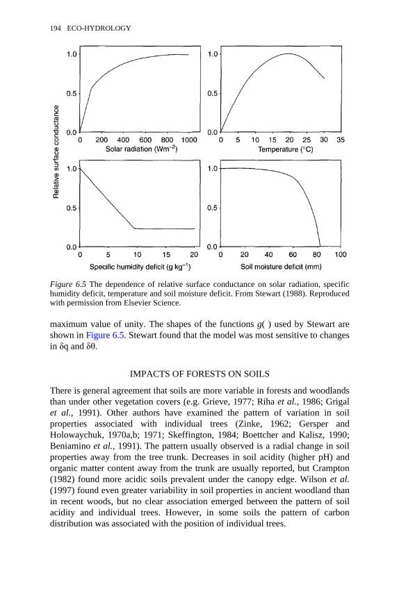
maximum value of unity. The shapes of the functions g( ) used by Stewart areshown in Figure 6.5. Stewart found that the model was most sensitive to changesin δq and δθ.
IMPACTS OF FORESTS ON SOILS
There is general agreement that soils are more variable in forests and woodlandsthan under other vegetation covers (e.g. Grieve, 1977; Riha et al., 1986; Grigalet al., 1991). Other authors have examined the pattern of variation in soilproperties associated with individual trees (Zinke, 1962; Gersper andHolowaychuk, 1970a,b; 1971; Skeffington, 1984; Boettcher and Kalisz, 1990;Beniamino et al., 1991). The pattern usually observed is a radial change in soilproperties away from the tree trunk. Decreases in soil acidity (higher pH) andorganic matter content away from the trunk are usually reported, but Crampton(1982) found more acidic soils prevalent under the canopy edge. Wilson et al.(1997) found even greater variability in soil properties in ancient woodland thanin recent woods, but no clear association emerged between the pattern of soilacidity and individual trees. However, in some soils the pattern of carbondistribution was associated with the position of individual trees.
Figure 6.5 The dependence of relative surface conductance on solar radiation, specifichumidity deficit, temperature and soil moisture deficit. From Stewart (1988). Reproducedwith permission from Elsevier Science.
194 ECO-HYDROLOGY
The concentration of carbon content in soils close to the tree is presumablybecause of the predominance of litter, both leaves and branches, falling close totrees. The explanation for the pattern of pH will be the redistribution of rainfallby the canopies of the trees. In some tree species there is a considerableconcentration of throughfall as stemflow. Species with smooth bark surfacessuch as beech may transport as much as 12 percent of precipitation as stemflow,whereas pine transfers less than 2 percent (Kittredge, 1948). Examples of highcontributions of stemflow to throughfall are also observed in tropical rain forests(Bruijnzeel, 1990). Stemflow may also concentrate water near to the roots of semi-arid species such as Acacia aneura (Pressland, 1973). In contrast, other treespecies shed considerable throughfall from their canopy edges (Crampton, 1982;Darnhofer et al., 1989).
Where there is a significant spatial heterogeneity of throughfall, there will beconsequences for the chemistry and water content of the soil. Forexample, chemicals deposited previously on the canopy and branches as drydeposition are dissolved by rainwater and added to the soil via localisedthroughfall or stemflow. As well as the impact that these chemicals have onlocalised activity in the soil (which depends on chemical species delivered fromthe canopy), there is also the question of calculating soil nutrient budgets and theneed, therefore, for adequate sampling of throughfall when it is delivered in aspatially heterogeneous way. Stemflow may have special significance indelivering potassium, a major plant nutrient, to the area around certain smooth-barked trees, because it is readily leached from the foliage (Gersper andHolowaychuk, 1971).
The heterogeneity in throughfall and associated chemical constituentsproduced below a woodland canopy consisting of different tree species, tree agesand canopy geometries is likely to have an impact on the species constituting theunderstorey (Simmons and Buckley, 1992).
The redistribution of rainfall and associated chemicals by forest canopies, thelocation of roots in the forest floor and the presence of an understorey havepractical relevance to the quality of water draining from different forests.Kinniburgh and Trafford (1996) considered that a localised rooting pattern,absence of understorey and wind-throw disturbance were responsible for higherpore water concentrations of NO, below a beech stand compared with an ashstand. The ash stand, on the other hand, was thought to have an extensive rootsystem and had a vigorous understorey (dog’s mercury) with a spreadingrhizomatous root system. Kinniburgh and Trafford also observed higherconcentration in the pore water within 50 m of the edge within the beech woodand also found that the the subsoil water content was lower over this region thanfurther inside the wood. Because of the very efficient aerodynamic mixing of theatmosphere with the tree canopies there is enhanced deposition of chemicals atthe forest edge. Water use is also likely to be higher, because the aerodynamicconditions will also favour larger interception losses, and the greaterconcentration of leaf area at the edge will mean higher transpiration. The
PLANTS AND WATER IN FORESTS AND WOODLANDS 195
processes at woodland edges are receiving more attention in a number ofEuropean countries because of the increased planting of small areas ofwoodlands and concerns about chemical deposition. However, the increasedwater use at the forest edge may also be important in minimising drainage, whichotherwise would transport chemicals from the forest to groundwater or streams.
A further consequence of the chemical composition and pH of stemflow wasreported by Chappell et al. (1996), who observed a lower hydraulic conductivityin the surface soil horizons closer to trees than some distance away. This effectwas thought to be due to acid stemflow water mobilising clay particles, whichseal fine pores in the clay close to the tree trunk. These authors also believe thatthe mass of the tree has a compacting effect, which is greatest near to the tree’saxis.
Some early studies showed a decrease in stemflow as a forest becomesolder (Delfs, 1967; Helvey, 1967), but in other studies there was no age effect onstemflow as a percentage of gross rainfall (Brown and Parker, 1970). There are anumber of features of older trees that might contribute to a reduction in stemflow.Tree trunks will tend to become less smooth or covered with lichens or mosses,and more distorted with age, and the canopy will comprise a greater percentageof longer, heavier branches that are not angled upwards. It seems reasonable toassume that the young, short and upright branches at the tops of trees directwater to the central trunk, from where it is likely to reach the ground as stemflow.The older, lower branches in tree canopies are larger and more complex. Theyare more often horizontal or may even curve downwards away from the stem. Asthe fraction of the canopy having an upright structure is reduced, the proportionof throughfall occurring as stemflow is likely to fall. Using a 9 m tall Douglas firtree, Hutchinson and Roberts (1981) found that 69 percent of the stemflow camefrom the upper half of the canopy and explained this distribution in terms ofdiffering branching angle geometry within the tree crown. It might, therefore, beexpected that some of the patterns of pH and chemical composition wouldchange as forests became older and stemflow became a smaller percentage of thethroughfall.
Despite the observations of reduced hydraulic conductivity of soil close totrees by Chappell et al. (1996), it is generally assumed that when stemflow waterreaches the base of the tree it can enter the soil readily along the outside of majorroots, which radiate outwards and downwards from the base of the tree. Thisinfiltration may be aided in dry conditions because of shrinkage of the roots toleave air gaps. As well as the infiltration along root channels at the bases oftrees, high infiltration rates are usually observed throughout undisturbed forests.The presence of leaf litter at the surface and live and dead root channels deeperdown is thought to play a key role in the high infiltration capacity and saturatedhydraulic conductivity of undisturbed forest soils (Beasley, 1976; Beven andGermann, 1982). Tracing experiments (Reynolds, 1966) and direct observation(Bonell and Gilmour, 1978) indicate the importance of live and dead root channelsfor water entry and transmission in forest soils. Gaiser (1952) estimated that
196 ECO-HYDROLOGY
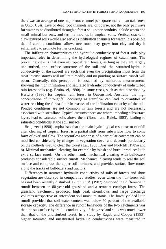
there was an average of one major root channel per square metre in an oak forestin Ohio, USA. Live or dead root channels are, of course, not the only pathwaysfor water to be distributed through a forest soil; other conduits include worm andsmall animal burrows, and termite mounds in tropical soils. Vertical cracks inclay-textured soils would also serve as infiltration channels for water. It is possiblethat if aerobic conditions allow, tree roots may grow into clay and dry itsufficiently to promote further cracking.
The infiltration characteristics and hydraulic conductivity of forest soils playimportant roles in determining the hydrological regimes of catchments. Theprevailing view is that even in tropical rain forests, as long as they are largelyundisturbed, the surface structure of the soil and the saturated hydraulicconductivity of the subsoil are such that even the precipitation input from themost intense storms will infiltrate readily and no ponding or surface runoff willoccur. Generally, this perception is sustained by numerous measurementsshowing the high infiltration and saturated hydraulic conductivity of undisturbedrain forest soils (e.g. Bruinzeel, 1990). In some cases, such as that described byHerwitz (1986) for tropical rain forest in Queensland, Australia, the highconcentration of throughfall occurring as stemflow can lead to quantities ofwater reaching the forest floor in excess of the infiltration capacity of the soil.Ponded conditions are not common in rain forests and are not necessarilyassociated with stemflow. Typical circumstances are where impeding subsurfacelayers lead to saturated soils above them (Bonell and Balek, 1993), leading tosaturated conditions at the soil surface.
Bruijnzeel (1990) emphasises that the main hydrological response to rainfallafter clearing of tropical forest is a partial shift from subsurface flow to someform of overland flow. The stormflow response of a particular catchment can bemodified considerably by changes in vegetation cover and depends particularlyon the methods used to clear the forest (Lal, 1983; Dias and Nortcliff, 1985a andb). Minimal mechanical clearing, for example by ‘slash and burn’, produces littleextra surface runoff. On the other hand, mechanical clearing with bulldozersproduces considerable surface runoff. Mechanical clearing tends to seal the soilsurface and compress the upper soil horizons, and provides surface flow routesalong the tracks of bulldozers and tractors.
Differences in saturated hydraulic conductivity of soils of forests and shortvegetation are observed in comparative studies, even when the non-forest soilhas not been recently disturbed. Burch et al. (1987) described the difference inrunoff between an 80-year-old grassland and a remnant eucalypt forest. Thegrassland catchment produced high peak stormflows and large dischargevolumes irrespective of antecedent soil moisture status. The forest yielded littlerunoff provided that soil water content was below 60 percent of the availablestorage capacity. The difference in runoff behaviour of the two catchments wasthat the subsurface hydraulic conductivity of the grassland soils was much lowerthan that of the undisturbed forest. In a study by Ragab and Cooper (1993),higher saturated and unsaturated hydraulic conductivities were measured in
PLANTS AND WATER IN FORESTS AND WOODLANDS 197

woodland than in permanent pasture. Both woodland and permanent pasture hadhigher hydraulic conductivities than arable soil.
There will be variation in soil moisture conditions determined by the spatialdistribution of throughfall and infiltration characteristics. Clearly the live anddead root channels and other fissures described above contribute to the highhydraulic conductivity of forest soils and allow water to be delivered to deephorizons. This may provide an advantage to trees, particularly in semi-aridregions, as some deeply placed water will be out of reach of shallow-rootedplants, allowing the trees competitive advantage.
In addition to variations in the lateral and vertical distribution of soil watercaused by heterogeneity of throughfall and infiltration, there will be patterns ofsoil moisture distribution caused by variations in root uptake. The traditionalview of tree root distribution in forests is that it substantially exceeds shortvegetation rooting depth and lateral extent from individual plants. Recently, therehave been comprehensive reviews of maximum rooting depths (Canadell et al.,1996) and vertical root distributions (Jackson et at., 1996) of global vegetationtypes. From these two papers it can be concluded that trees of temperatebroadleaf and coniferous forests, tropical rain forests and shrubs, especially thosein arid or semi-arid areas, have the deepest roots. Additionally, most woodyvegetation has about 50 percent of roots in the upper 30 cm of soil. An exceptionis boreal forest, which along with tundra and grassland has between 80 and 90percent of its roots in the upper 30 cm of soil. The lateral spread of roots fromwoody plants clearly varies with the climatic zone. In humid forests, the lateralspread of shallow roots is limited; roots are confined within the canopy area(Kellman, 1979). In semiarid regions, the area exploited by lateral roots extendsbeyond the edge of the canopy, sometimes by a considerable distance, asindicated by studies in Australia of Acacia pendula (Story, 1967) and inCalifornia on chaparral shrubs (Kummerow et al., 1977) (for more informationon dryland plants, see Chapter 4).
Where trees and shorter vegetation grow together it is usually the case thatboth will have roots in the upper soil layers, while only the trees will have rootsin the deeper layers (fireman and Kessler, 1995). This type of situation is foundin a wide range of woody vegetation, e.g. semi-arid savannah woodlands andtemperate broadleaf woodlands with an understorey of shrubs and herbs. Whenthe root distribution is of this form, competition between the trees and shortvegetation for the soil water resources in the upper soil layers is likely to besevere. Nevertheless, despite this competition for soil moisture from the upper soilhorizons, there is evidence that, in semi-arid woodlands at least, growth of shortherbaceous vegetation is greater under trees than in the open (Scholes andArcher, 1997). There are a number of plausible explanations why this should beso. One explanation is that below trees there is a greater availability of waterbecause the soil has a lower bulk density and higher porosity. Additionally, thetree cover reduces radiation load on the vegetation below and, therefore, reducesevaporative demand (Joffre and Rambal, 1988). Under the trees the leaf
198 ECO-HYDROLOGY

temperatures of grasses and herbs are probably 2–3 °C lower than in the open, adifference which may mean that physiological conditions are closer to optimal.Another factor that may contribute to improved growth of short vegetation undertrees may be additional water provided to the surface soil horizons by tree rootsaccessing soil water deep in the soil profile. This water is transported upwardsand passes out of the plant into dry surface soil horizons when the stomata areclosed at night. Evidence for this process, termed ‘hydraulic lift’ (see Chapter 2)was found by Richards and Caldwell (1987) working with a sagebrush(Artemisia tridentata) community in the semi-arid regions of the USA.They observed a regular pattern of soil drying at 35–80 cm depth during thedaytime followed by wetting at night. This wetting could not be explained bytransfer through the soil alone. Although the amounts of water that were movedto the upper soil layers were small (about 20–30 mm in a dry season), they maybe important for plant survival and preventing the drying out of surface roots.
In normal conditions, differences in transpiration both between broadleaf andconiferous forests and within the two groups are small (Table 6.2), but in somecircumstances differences between species may occur that will create differencesin soil moisture content. These situations will probably occur when conditionsare less suitable for one species while another species is largely unaffected or canadapt to the prevailing situation. An example that has practical significance inforestry is the response of different species on waterlogged, poorly aerated peatysoils, where the presence of trees may have substantial impacts on the soil. Thepotential for drying of peat in the lower soil levels is likely to be greater for treeswith deeper root systems. King et al. (1986) reported that peaty soils were betteraerated and had lower water tables in summer under lodgepole pine comparedwith sitka spruce. It is known that the roots of lodgepole pine can survivewaterlogging, while those of spruce are intolerant of such conditions (Coutts andPhillipson, 1978).
CASE STUDIES
Case study 1: Temperate coniferous forest, Thetford Chase,UK
The site
The Scots pine (Pinus sylvestris L.) stand was in Thetford Forest (52°25′N; 0°39′E) and was planted in 1931. In 1976, there were 600 trees ha−1, with the averageheight being about 16 m. The soil was sand, approximately 1 m deep, overlying2–3 m of glacial till over pure chalk. Tree roots were found throughout this depthand some reached the chalk (Roberts, 1976b). There was a bracken (Pteridiumaquilinum (L.) Kuhn.) understorey, the rhizomes of which penetrated to a depth
PLANTS AND WATER IN FORESTS AND WOODLANDS 199
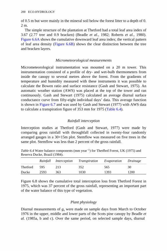
of 0.5 m but were mainly in the mineral soil below the forest litter to a depth of 0.2 m.
The simple structure of the plantation at Thetford had a total leaf area index of3.67 (2.77 tree and 0.9 bracken) (Beadle et al., 1982; Roberts et al., 1980).Figure 6.6A shows the cumulative downward leaf area index; the vertical patternof leaf area density (Figure 6.6B) shows the clear distinction between the treeand bracken layers.
Micrometeorological measurements
Micrometeorological instrumentation was mounted on a 20 m tower. Thisinstrumentation consisted of a profile of dry- and wet-bulb thermometers frominside the canopy to several metres above the forest. From the gradients oftemperature and humidity measured with these instruments it was possible tocalculate the Bowen ratio and surface resistance (Gash and Stewart, 1975). Anautomatic weather station (AWS) was placed at the top of the tower and rancontinuously. Gash and Stewart (1975) calculated an average diurnal surfaceconductance curve from fifty-eight individual days’ data. This average functionis shown in Figure 6.7 and was used by Gash and Stewart (1977) with AWS datato calculate a transpiration figure of 353 mm for 1975 (Table 6.4).
Rainfall interception
Interception studies at Thetford (Gash and Stewart, 1977) were made bycomparing gross rainfall with throughfall collected in twenty-four randomlyarranged gauges in a 30×15m plot. Stemflow was measured on five trees in thesame plot. Stemflow was less than 2 percent of the gross rainfall.
Table 6.4 Water balance components (mm year−1) for Thetfbrd Forest, UK (1975) andReserva Ducke, Brazil (1984).
Rainfall Interception Transpiration Evaporation Drainage
Thetford 595 213 352 565 30Ducke 2593 363 1030 1393 1200
Figure 6.8 shows the cumulative total interception loss from Thetford Forest in1975, which was 37 percent of the gross rainfall, representing an important partof the water balance of this type of vegetation.
Plant physiology
Diurnal measurements of gs were made on sample days from March to October1976 in the upper, middle and lower parts of the Scots pine canopy by Beadle etal. (1985a, b and c). Over the same period, on selected sample days, diurnal
200 ECO-HYDROLOGY
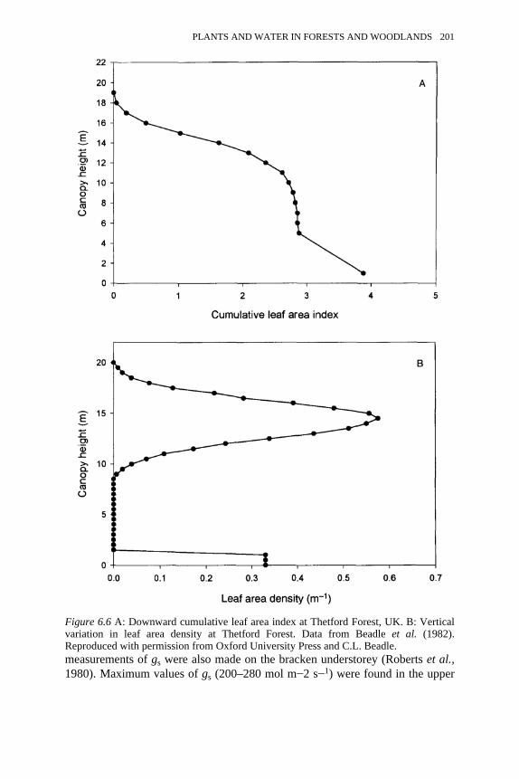
measurements of gs were also made on the bracken understorey (Roberts et al.,1980). Maximum values of gs (200–280 mol m−2 s−1) were found in the upper
Figure 6.6 A: Downward cumulative leaf area index at Thetford Forest, UK. B: Verticalvariation in leaf area density at Thetford Forest. Data from Beadle et al. (1982).Reproduced with permission from Oxford University Press and C.L. Beadle.
PLANTS AND WATER IN FORESTS AND WOODLANDS 201
part of the tree canopy, and values declined towards the lower levels of thecanopy. The maximum values occurred around mid-morning and declinedthereafter. Except when temperatures were below 10 °C or light levels were low,at dawn and dusk, changes in gs were related mainly to changes in air humiditydeficit; low stomatal conductances were associated with high air humiditydeficits (Figure 6.9). Despite the measurements being made in the drought year of1976, gs showed no relationship with variation in leaf water potential (ψ1).
Maximum values of gs in the bracken canopy were around 140 mmol m−2 s−1.Even in the dry summer of 1976, gs of the bracken was not strongly influencedby low soil water content, and the bracken was much less sensitive to airhumidity deficit than were the pine trees. Transpiration from the bracken canopyas a percentage of the total forest transpiration was typically between 20 and 30percent. However, in periods when high air humidity deficits prevailed, whichreduced gs of the trees more than that of the bracken, the percentage contributionof bracken transpiration to the forest total could exceed 50 percent (Figure 6.10).
Figure 6.7 Average diurnal curves of canopy conductance for the forest at the ReservaDucke, Manaus, and Thetford Forest in a normal and a dry year. Redrawn from Shuttleworth(1989). Reproduced with permission from the Royal Society of London andW.J.Shuttleworth.
202 ECO-HYDROLOGY
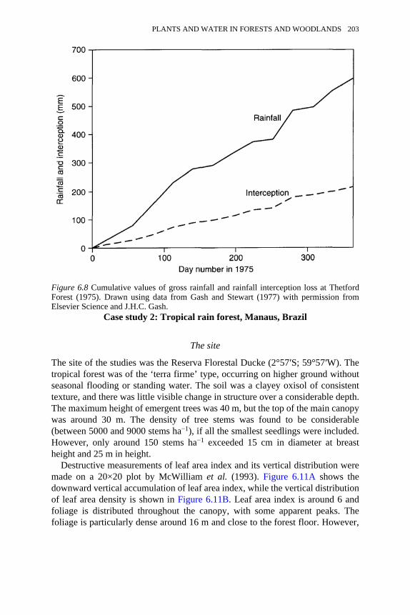
Case study 2: Tropical rain forest, Manaus, Brazil
The site
The site of the studies was the Reserva Florestal Ducke (2°57′S; 59°57′W). Thetropical forest was of the ‘terra firme’ type, occurring on higher ground withoutseasonal flooding or standing water. The soil was a clayey oxisol of consistenttexture, and there was little visible change in structure over a considerable depth.The maximum height of emergent trees was 40 m, but the top of the main canopywas around 30 m. The density of tree stems was found to be considerable(between 5000 and 9000 stems ha−1), if all the smallest seedlings were included.However, only around 150 stems ha−1 exceeded 15 cm in diameter at breastheight and 25 m in height.
Destructive measurements of leaf area index and its vertical distribution weremade on a 20×20 plot by McWilliam et al. (1993). Figure 6.11A shows thedownward vertical accumulation of leaf area index, while the vertical distributionof leaf area density is shown in Figure 6.11B. Leaf area index is around 6 andfoliage is distributed throughout the canopy, with some apparent peaks. Thefoliage is particularly dense around 16 m and close to the forest floor. However,
Figure 6.8 Cumulative values of gross rainfall and rainfall interception loss at ThetfordForest (1975). Drawn using data from Gash and Stewart (1977) with permission fromElsevier Science and J.H.C. Gash.
PLANTS AND WATER IN FORESTS AND WOODLANDS 203
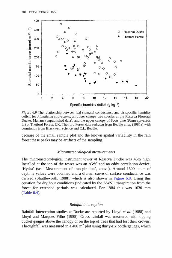
because of the small sample plot and the known spatial variability in the rainforest these peaks may be artifacts of the sampling.
Micrometeorological measurements
The micrometeorological instrument tower at Reserva Ducke was 45m high.Installed at the top of the tower was an AWS and an eddy correlation device,‘Hydra’ (see ‘Measurement of transpiration’, above). Around 1500 hours ofdaytime values were obtained and a diurnal curve of surface conductance wasderived (Shuttleworth, 1988), which is also shown in Figure 6.8. Using thisequation for dry hour conditions (indicated by the AWS), transpiration from theforest for extended periods was calculated. For 1984 this was 1030 mm(Table 6.4).
Rainfall interception
Rainfall interception studies at Ducke are reported by Lloyd et al. (1988) andLloyd and Marques Filho (1988). Gross rainfall was measured with tippingbucket gauges above the canopy or on the top of trees that had lost their crowns.Throughfall was measured in a 400 m2 plot using thirty-six bottle gauges, which
Figure 6.9 The relationship between leaf stomatal conductance and air specific humiditydeficit for Piptadenia suaveolens, an upper canopy tree species at the Reserva FlorestalDucke, Manaus (unpublished data), and the upper canopy of Scots pine (Pinus sylvestrisL.) at Thetford Forest, UK. Thetford Forest data redrawn from Beadle et al. (1985a) withpermission from Blackwell Science and C.L. Beadle.
204 ECO-HYDROLOGY
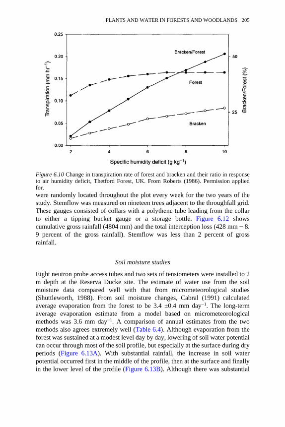
were randomly located throughout the plot every week for the two years of thestudy. Stemflow was measured on nineteen trees adjacent to the throughfall grid.These gauges consisted of collars with a polythene tube leading from the collarto either a tipping bucket gauge or a storage bottle. Figure 6.12 showscumulative gross rainfall (4804 mm) and the total interception loss (428 mm − 8.9 percent of the gross rainfall). Stemflow was less than 2 percent of grossrainfall.
Soil moisture studies
Eight neutron probe access tubes and two sets of tensiometers were installed to 2m depth at the Reserva Ducke site. The estimate of water use from the soilmoisture data compared well with that from micrometeorological studies(Shuttleworth, 1988). From soil moisture changes, Cabral (1991) calculatedaverage evaporation from the forest to be 3.4 ±0.4 mm day−1. The long-termaverage evaporation estimate from a model based on micrometeorologicalmethods was 3.6 mm day−1. A comparison of annual estimates from the twomethods also agrees extremely well (Table 6.4). Although evaporation from theforest was sustained at a modest level day by day, lowering of soil water potentialcan occur through most of the soil profile, but especially at the surface during dryperiods (Figure 6.13A). With substantial rainfall, the increase in soil waterpotential occurred first in the middle of the profile, then at the surface and finallyin the lower level of the profile (Figure 6.13B). Although there was substantial
Figure 6.10 Change in transpiration rate of forest and bracken and their ratio in responseto air humidity deficit, Thetford Forest, UK. From Roberts (1986). Permission appliedfor.
PLANTS AND WATER IN FORESTS AND WOODLANDS 205
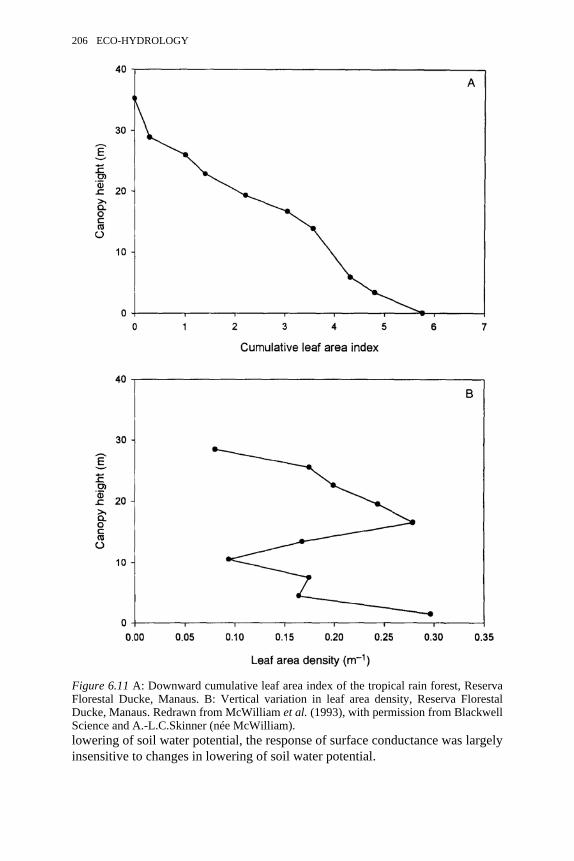
lowering of soil water potential, the response of surface conductance was largelyinsensitive to changes in lowering of soil water potential.
Figure 6.11 A: Downward cumulative leaf area index of the tropical rain forest, ReservaFlorestal Ducke, Manaus. B: Vertical variation in leaf area density, Reserva FlorestalDucke, Manaus. Redrawn from McWilliam et al. (1993), with permission from BlackwellScience and A.-L.C.Skinner (née McWilliam).
206 ECO-HYDROLOGY
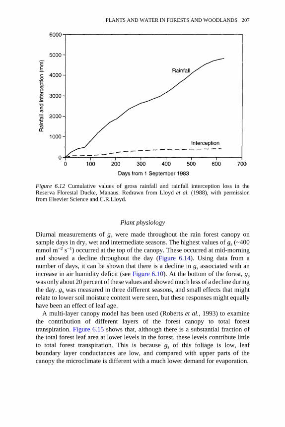
Plant physiology
Diurnal measurements of gs were made throughout the rain forest canopy onsample days in dry, wet and intermediate seasons. The highest values of gs (~400mmol m−2 s−1) occurred at the top of the canopy. These occurred at mid-morningand showed a decline throughout the day (Figure 6.14). Using data from anumber of days, it can be shown that there is a decline in gs associated with anincrease in air humidity deficit (see Figure 6.10). At the bottom of the forest, gswas only about 20 percent of these values and showed much less of a decline duringthe day. gs was measured in three different seasons, and small effects that mightrelate to lower soil moisture content were seen, but these responses might equallyhave been an effect of leaf age.
A multi-layer canopy model has been used (Roberts et al., 1993) to examinethe contribution of different layers of the forest canopy to total foresttranspiration. Figure 6.15 shows that, although there is a substantial fraction ofthe total forest leaf area at lower levels in the forest, these levels contribute littleto total forest transpiration. This is because gs of this foliage is low, leafboundary layer conductances are low, and compared with upper parts of thecanopy the microclimate is different with a much lower demand for evaporation.
Figure 6.12 Cumulative values of gross rainfall and rainfall interception loss in theReserva Florestal Ducke, Manaus. Redrawn from Lloyd et al. (1988), with permissionfrom Elsevier Science and C.R.Lloyd.
PLANTS AND WATER IN FORESTS AND WOODLANDS 207
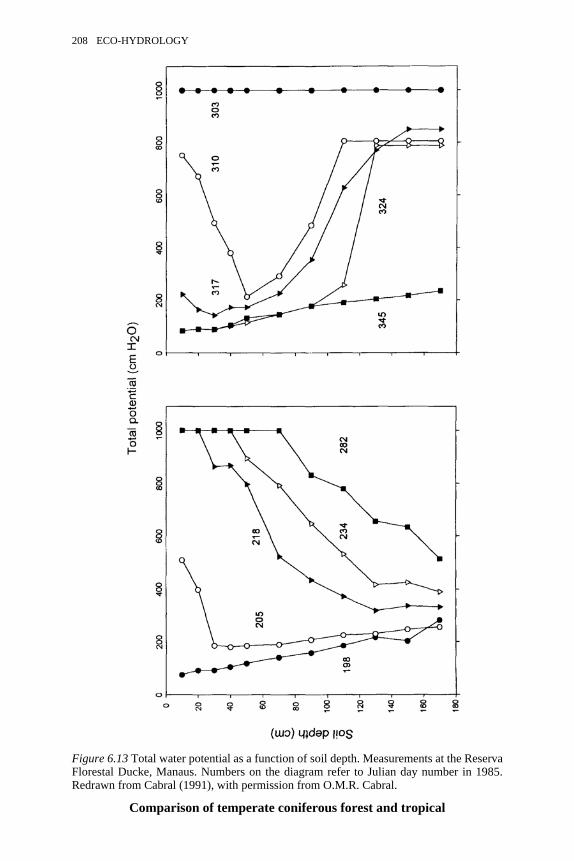
Comparison of temperate coniferous forest and tropical
Figure 6.13 Total water potential as a function of soil depth. Measurements at the ReservaFlorestal Ducke, Manaus. Numbers on the diagram refer to Julian day number in 1985.Redrawn from Cabral (1991), with permission from O.M.R. Cabral.
208 ECO-HYDROLOGY

rain forest
A major hydrological difference between these types of forest is in rainfallinterception as a percentage of gross rainfall. In Thetford, rainfall interception isaround 37 percent of gross rainfall, whereas in the tropical rain forest less than 9percent of incident rainfall is lost as interception. This difference is due to thevery different nature of rainfall in temperate and tropical regions. In temperateregions, particularly when rainfall is frontal, rainstorms are frequent, light inintensity and often of long duration; canopies are very effectively wetted bysmall raindrops. Evaporation from the wetted canopy can take place during therainstorms if the atmosphere is not fully saturated. Under these circumstances,interception losses can constitute a considerable percentage of incident rainfall: afact of both practical and ecological importance when forests, particularlyevergreen conifers, are planted. The situation in tropical rain forests is quite different; rainstorms are intense andof short duration, and raindrops tend to be large. Under these circumstances,canopies wet slowly and there is also less opportunity for evaporation during theshort storm. The high kinetic energy of raindrops in tropical conditions is animportant factor in rain splash erosion. In undisturbed rain forest canopies, thereis not a serious problem because of the dissipation of kinetic energy by the manylayers of vegetation. In tropical forest plantations with no significantundergrowth, however, there is no barrier to the raindrops as they fall from the
Figure 6.14 Diurnal variation in stomatal conductance of some of the species around thesampling tower at Reserva Ducke, Manaus. 1) Piptadenia suaveolens at 33 m; 2) Licaniamicrantha at 25.6 m; 3) Naucleopsis glabra at 17 m; 4) Scheelea spp. at 3 m. FromRoberts et al. (1990), with permission from Blackwell Science.
PLANTS AND WATER IN FORESTS AND WOODLANDS 209
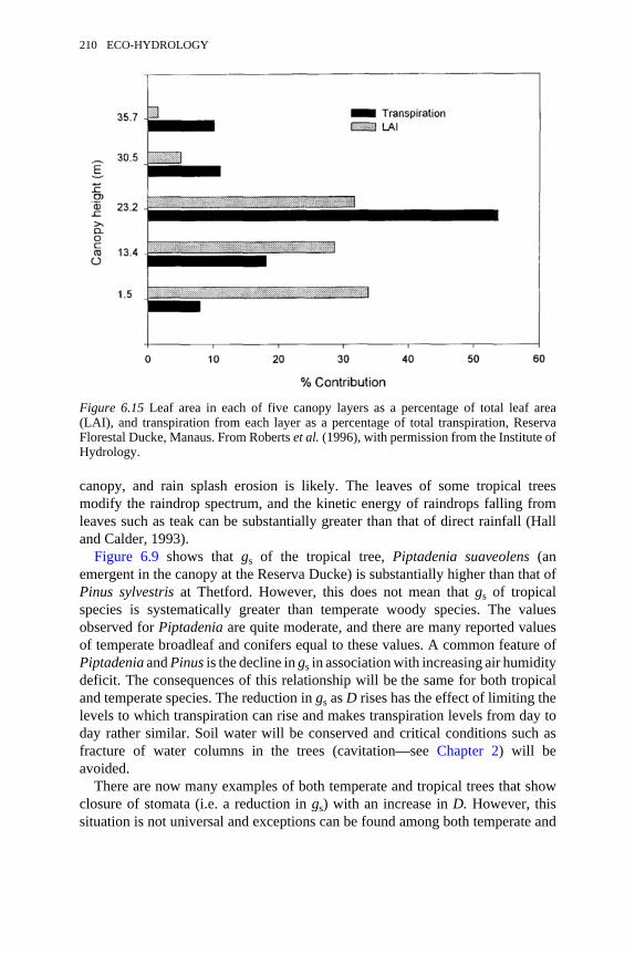
canopy, and rain splash erosion is likely. The leaves of some tropical treesmodify the raindrop spectrum, and the kinetic energy of raindrops falling fromleaves such as teak can be substantially greater than that of direct rainfall (Halland Calder, 1993).
Figure 6.9 shows that gs of the tropical tree, Piptadenia suaveolens (anemergent in the canopy at the Reserva Ducke) is substantially higher than that ofPinus sylvestris at Thetford. However, this does not mean that gs of tropicalspecies is systematically greater than temperate woody species. The valuesobserved for Piptadenia are quite moderate, and there are many reported valuesof temperate broadleaf and conifers equal to these values. A common feature ofPiptadenia and Pinus is the decline in gs in association with increasing air humiditydeficit. The consequences of this relationship will be the same for both tropicaland temperate species. The reduction in gs as D rises has the effect of limiting thelevels to which transpiration can rise and makes transpiration levels from day today rather similar. Soil water will be conserved and critical conditions such asfracture of water columns in the trees (cavitation—see Chapter 2) will beavoided.
There are now many examples of both temperate and tropical trees that showclosure of stomata (i.e. a reduction in gs) with an increase in D. However, thissituation is not universal and exceptions can be found among both temperate and
Figure 6.15 Leaf area in each of five canopy layers as a percentage of total leaf area(LAI), and transpiration from each layer as a percentage of total transpiration, ReservaFlorestal Ducke, Manaus. From Roberts et al. (1996), with permission from the Institute ofHydrology.
210 ECO-HYDROLOGY
tropical species, with important hydrological and ecological consequences. Halland Allen (1997) describe results of physiological behaviour and water use ofpoplar short rotation coppice (SRC). Unlike the tree species examined here, SRCdoes not show a reduction of gs with D, and high values of gs can be maintainedthroughout the day if solar radiation is adequate and soil water is not limiting.Under these circumstances, transpiration rates as high as 10 mm day−1 have beenobserved. Findings such as these may influence decisions on whether SRC is asuitable option where water resources might be compromised by the high wateruse of SRC.
Results from studies of eucalyptus in India have also shown that the speciesthat are typically planted, E. camadulensis and E. tereticornis, exhibit high gs,which is not reduced by the dryness of the atmosphere. When unrestricted bysoil water deficits, daily water use can be up to 6 mm day−1. However, gs canbecome limited by low soil water content in dry seasons if rooting depth islimited (Roberts et al., 1992), and transpiration rates can fall to around 1 mm day−1. A very important finding from studies in India has been the indication that atsome sites rooting is not restricted and eucalypts can exploit deeper and deepersoil water to sustain their transpiration. Calder et al. (1997) have shown that insome locations in south India annual water use substantially exceeds the rainfall,causing serious concern for the sustainability of large tracts of eucalyptplantations. An acceptable alternative seems to be a rotational patchworkdistribution of eucalypt in the landscape alternating with agricultural crops,which will allow deep soil water to be replenished.
CONCLUDING REMARKS
This chapter has tended to concentrate on evaporation processes in a selection offorest types. Detailed processes in soils have not been addressed, not becausethey are unimportant but because arguably the differences in the hydrology ofdifferent forests are more related to processes in the vegetation itself. For pastgenerations of process hydrologists investigating forests, a key problem was thelack of techniques and equipment to provide useful data on the evaporationprocess. Now this seems less of a problem; we can measure leaf gas exchange,whole tree transpiration or stand gas exchange almost routinely withcommercially available equipment. We also seem to have a good understandingof the interception process and, even though measurement techniques have notadvanced, a better idea of the amount of replication that is required. Interceptionmodelling even for sparse canopies now seems to be based on a robust, physicalunderstanding.
Notwithstanding the brief discussion of forest soils, there are a number ofimportant impacts that trees have on soils. Deep litter layers and permeable soilsin forests ensure rapid and deep infiltration of water. In contrast to areas withshort, shallow-rooted vegetation, the hydrological responses of forested landswill show little or no surface runoff and, because of reserves of water in deep
PLANTS AND WATER IN FORESTS AND WOODLANDS 211
soil layers, sustained streamflow in dry periods. Another key impact of trees onsoil is their influence on chemical composition and the variability of chemicalcomposition. Compared with aerodynamically smoother, short vegetation thereis enhanced deposition, in dry conditions, of chemicals onto the crowns of treesfrom the atmosphere. Additional chemicals arrive in the rain, and these arefurther concentrated on the canopy by the evaporation of intercepted water. Thechemical composition of throughfall water can influence physical soilcharacteristics, such as hydraulic conductivity, by altering the integrity of clayparticles. In addition, variation in throughfall chemistry can influence thepatterns of woodland flora by altering the distribution of specific siterequirements. There is some evidence that root uptake, coupled with high rootdensities in surface soils of forests, can prevent chemicals leaching from theecosystem, but more detailed study of rooting patterns and the influence of theseon chemistry of drainage waters is required.
Some important remaining problems relate to the scale at which process data arecollected (see Chapter 3; Stewart et al., 1996; van Gardingen et al., 1997). Ofparticular interest is the effect of forests on climate, yet only in passing has thischapter referred to this research issue. The pressing need is for moremeasurement and modelling studies of the influence of forests on hydrologicaland climatological processes at the scale of a few to tens of kilometres.
Attention has been drawn to high interception loss, particularly in temperateconifer forests. On the other hand, in tropical forests the interception losses areperhaps surprisingly low as a percentage of rainfall, but we have plausibleexplanations of why this is. Temperate and tropical forests differ markedly ininterception losses as a percentage of gross rainfall but, in sharp contrast, thereare similarities in the control of transpiration. The important common feature isthe reduction of stomatal conductance with increasing air humidity deficit. Themechanisms behind this behaviour are still debated, but the net effect is aconservative transpiration rate and a similarity in transpiration from day to day.The response of stomata to humidity deficit and conservative transpirationprobably delays the onset of stomatal closure due to deficits of soil moisture.Clearly, the mechanisms behind such a widely occurring phenomenon deservemore study. The low transpiration rates of tropical forests seem, at first,surprising but we are becoming more aware of large year to year variation inrainfall in tropical forest regions. Thus, low transpiration rates may be a strategyfor conserving water. Only in recent years has the existence of deep roots intropical forests become known. However, at the moment the purpose of thesedeep roots is not clear, unless they provide an insurance in the driest years.
The daily transpiration rates of tropical forests are modest and hardly exceedthose of temperate forests. As well as feedbacks between the environment andstomatal conductance, the structure of the tropical forest itself contributes tolimited transpiration. Although the leaf area of a tropical forest is nearly doublethat of many temperate forests, substantial amounts of this foliage are in parts ofthe canopy where conditions for promoting transpiration are not optimal.
212 ECO-HYDROLOGY

Stomata are only partially open, wind speeds are low and humidity is close tosaturation. Perhaps as little as fifteen years ago we knew very little about thehydrology, micrometeorology and physiology of tropical forests. Through asustained research effort by a number of groups we now know a lot more, butclearly there is more to learn. Nevertheless, it is perhaps time for attention to beturned to forest types about which we know very little. These are savannahs,boreal forests and semi-arid and mediterranean woodlands.
REFERENCES
Beadle, C.L., Talbot, H. and Jarvis, P.G. (1982) Canopy structure and leaf area index in amature Scots pine forest, Forestry 55:105–123.
Beadle, C.L., Neilson, R.E., Talbot, H. and Jarvis, P.G. (1985a) Stomatal conductance andphotosynthesis in a mature Scots pine forest. I. Diurnal, seasonal and spatial variationin shoots, Journal of Applied Ecology 22:557–571.
Beadle, C.L., Jarvis, P.G., Talbot, H. and Neilson, R.E. (1985b) Stomatal conductance andphotosynthesis in a mature Scots pine forest. II. Dependence on environmentalvariables of single shoots, Journal of Applied Ecology 22:573–586.
Beadle, C.L., Talbot, H., Neilson, R.E. and Jarvis, P.G. (1985c) Stomatal conductance andphotosynthesis in a mature Scots pine forest. III. Variation in canopy conductanceand canopy photosynthesis, Journal of Applied Ecology 22:587–595.
Beasley, R.S. (1976) Contribution of subsurface flow from the upper slopes of forestedwatersheds to channel flow, Soil Science Society of America Journal 40: 955–957.
Bell, J.P. (1987) Neutron Probe Practice. IH Report No. 19, Institute of Hydrology,Wallingford, UK.
Bell, J.P., Dean, T.J. and Hodnett, M.G. (1987) Soil moisture measurement by animproved capacitance technique. Part II: Field techniques, evaluation and calibration,Journal of Hydrology 93:79–90.
Beniamino, F., Ponge, J.F. and Arpin, P. (1991) Soil acidification under the crown of oaktrees. I. Spatial distribution, Forest Ecology and Management 40: 221–232.
Beven, K.J. and Germann, P.F. (1982) Macropores and water flow in soils, WaterResources Research 18:1311–1325.
Black, T.A., Den Hartog, G., Neumann, H.H., Blanken, P.O., Yang, P.C., Russell, Nesic,Z., Lee, X., Chen, S.G., Staebler, R. and Novak, M.D. (1996) Annual cycles of watervapour and carbon dioxide fluxes in and above a boreal aspen forest , Global ChangeBiology 2:219–229.
Black, T.A. and Kelliher, F.M. (1989) Processes controlling understoreyevapotranspiration, Philosophical Transactions of the Royal Society, London B324:207–231.
Bobay, V. (1990) Influence d’une éclaircie sur le flux de sève et la transpiration de taillisde châtagnier, these de docteur en sciences, Université de Paris-Sud, Orsay. 218pp.
Boettcher, S.E. and Kalisz, P.J. (1990) Single-tree influence on soil properties in themountains of eastern Kentucky, Ecology 71:1365–1372.
Bonell, M. and Balek, J. (1993) Recent scientific developments and research needs inhydrological processes of the humid tropics, in M.Bonell, M.M.Hufschmidt and
PLANTS AND WATER IN FORESTS AND WOODLANDS 213
J.S.Gladwell (eds) Hydrology and Water Management in the Tropics, CambridgeUniversity Press, Cambridge, UK, pp. 167–260.
Bonell, M. and Gilmour, D.A. (1978) The development of overland flow in a tropical rainforest catchment, Journal of Hydrology 39:365–382.
Bouten, W., Schaap, M.G., Bakker, D.J. and Verstraten, J.M. (1992) Modelling soil waterdynamics in a forested ecosystem. I. A site specific evaluation, HydrologicalProcesses 6:435–444.
Bowen, I.S. (1926) The ratio of heat losses by conduction and by evaporation from anywater surface, Physical Review 27:779–787.
Brechtel, H.M. (1976) Influence of species and age of forest stands on evapotranspirationand ground water recharge in the Rhine-Main Valley, Proceedings of XVI IUFROWorld Congress, Oslo, Norway.
Bréda, N., Cochard, H., Dreyer, E. and Granier, A. (1993) Water transfer in a mature oakstand (Quercus petraea): seasonal evolution and effects of a severe drought,Canadian Journal of Forest Research 23:1136–1143.
Breman, H. and Kessler, J.-J. (1995) Woody Plants in Agro-ecosystems of Semi-aridRegions, Springer-Verlag, Berlin. 340 pp.
Brown, J.H., Jr and Barker, A.C., Jr (1970) An analysis of throughfall and stemflow inmixed oak stands, Water Resources Research 6:316–323.
Bruijnzeel, L.A. (1990) Hydrology of Moist Tropical Forests and Effects of Conversion: AState of Knowledge Review, UNESCO, Paris, and Free University, Amsterdam.224 pp.
Bruijnzeel, L.A. and Proctor, J. (1995) Hydrology and biogeochemistry of tropicalmontane cloud forests: what do we really know? in L.S.Hamilton, J.O.Juvik andF.N.Scatena (eds) Tropical Montane Cloud Forests Springer-Verlag, Berlin,pp. 38–78.
Bruijnzeel, L.A. and Wiersum, K.F. (1987) Rainfall interception by a youngAcacia auriculiformis A. Cunn. plantation forest in West Java, Indonesia: applicationof Gash’s analytical model, Hydrological Processes 1:309–319.
Burch, G.J., Bath, R.K., Moore, I.D. and O’Loughlin, E.M. (1987) Comparativehydrological behaviour of forested and cleared catchments in south-easternAustralia, Journal of Hydrology 90:19–42.
Cabral, O.M.R. (1991) Armazenagem da áqua num solo com floresta de terra firme e comseringal implantado, master’s thesis, Instituto Nacional de Pesquisas Espaciais,Brazil.
Calder, I.R. (1976) The measurement of water losses from a forested area using a‘natural’ lysimeter, Journal of Hydrology 30:311–325.
Calder. I.R. (1977) A model of transpiration and interception loss from a spruce forest inPlynlimon, central Wales, Journal of Hydrology 33:247–275.
Calder, I.R. (1986) A stochastic model of rainfall interception, Journal of Hydrology 89:65–71.
Calder, I.R. (1996) Dependence of rainfall interception on drop size: 1. Development ofthe two-layer stochastic model, Journal of Hydrology 185:363–378.
Calder, I.R. and Rosier, P.T.W. (1976) The design of large plastic sheet net rainfallgauges, Journal of Hydrology 30:403–405.
Calder, I.R., Hall, R.L., Rosier, P.T.W., Bastable, H.G. and Prasanna, K.T. (1996)Dependence of rainfall interception on drop size: 2. Experimental determination of
214 ECO-HYDROLOGY
the wetting functions and two-layer stochastic model parameters for five tropicalspecies, Journal of Hydrology 185:379–388.
Calder, I.R., Kariyappa, G.S., Srinivasalu, N.V. and Srinivasa Murthy, K.V. (1992)Deuterium tracing for the estimation of transpiration from trees. 1. Field calibration,Journal of Hydrology 130:17–25.
Calder, I.R., Rosier, P.T.W., Prasanna, K.T. and Parameswrappa, S. (1997) Eucalyptuswater use greater than rainfall input—a possible explanation from southern India,Hydrology and Earth System Sciences 1:249–256.
Calder, I.R., Wright, I.R. and Murdiyarso, D. (1986) A study of evaporation from tropicalrain forest—West Java, Journal of Hydrology 89:13–31.
Canadell, J., Jackson, R.B., Ehleringer, J.R., Mooney, H.A., Sala, O.E. and Schulze, E.-D.(1996) Maximum rooting depth of vegetation types at the global scale, Oecologia108:583–595.
Cermák, J., Jeník, J., Kucera, J. and Zídek, V. (1984) Xylem water flow in a crack willowtree (Salix fragilis L.) in relation to diurnal changes of environment, Oecologia 64:145–151.
Chappell, N., Stobbs, A., Ternan, L. and Williams, A. (1996) Localised impact of sitkaspruce (Picea sitchensis (Bong.) Carr.) on soil permeability, Plant and Soil 182:157–169.
Charney, J.G. (1975) Dynamics of deserts and drought in the Sahel, Quarterly Journal ofthe Royal Meteorological Society 101:193–202.
Chassagneux, P. and Choisnel, E. (1987) Modélisation de l’évaporation globale d’uncouvert forestier. II. Calibrages et résultats du modèle, Annales des SciencesForestières 44:171–188.
Courts, M.P. and Phillipson, J.J. (1978) Tolerance of tree roots to waterlogging. I.Survival of sitka spruce and lodgepole pine, New Phytologist 80:63–69.
Crampton, C.B. (1982) Podzolization of soils under individual tree canopies insouthwestern British Colombia, Canada, Geoderma 28:57–61.
Croft, A.R. and Monninger, L.V. (1953) Evapotranspiration and other water losses onsome aspen forest types in relation to water available for stream flow, Transactions ofthe American Geophysical Union 34:563–574.
Culf, A.D., Allen, S.J., Gash, J.H.C., Lloyd, C.R. and Wallace, J.S. (1993) Energy and waterbudgets of an area of patterned woodland in the Sahel, Agricultural and ForestMeteorology 66:65–80.
Czarnowski, M.S. and Olszewski, J.L. (1970) Number and spacing of rainfall gauges indeciduous forest stand, Oikos 21:48–51.
Darnhofer, T., Gatama, D., Huxley P.A. and Akunda, E. (1989) The rainfall distributionat a tree/crop interface, W.S.Reifsnyder and T.O.Darnhofer (eds) in Meteorology andAgroforestry, ICRAF, Nairobi, pp. 371–382.
Dean, T.J., Bell, J.P. and Baty, A.J.B. (1987) Soil moisture measurement by an improvedcapacitance technique. Part I: Sensor design and performance, Journal of Hydrology93:67–78.
Delfs, J. (1967) Interception and stemflow in stands of Norway spruce and beech in WestGermany, in W.E.Sopper and H.W.Lull (eds) International Symposium of ForestHydrology, Pergamon Press, New York, pp. 179–185.
Dias, A.C.C.P. and Nortcliff, S. (1985a) Effects of tractor passes on the physicalproperties of an oxisol in the Brazilian Amazon, Tropical Agriculture (Trinidad) 62:137–141.
PLANTS AND WATER IN FORESTS AND WOODLANDS 215
Dias, A.C.C.P. and Nortcliff, S. (1985b) Effects of two land clearing methods on thephysical properties of an oxisol in the Brazilian Amazon, Tropical Agriculture(Trinidad) 62:202–212.
Dietrich, W.E., Windsor, D.M. and Dunne, T. (1982) Geology, climate and hydrology ofBarro Colorado Island, in E.Leigh, A.S.Rand and D.M.Windsor (eds) The Ecology ofa Tropical Forest, Smithsonian Institution, Washington DC, pp. 21–46.
Dolman, A.J. (1987) Summer and winter rainfall interception in an oak forest. Predictionswith an analytical and a numerical simulation model, Journal of Hydrology 90:1–9.
Dugas, W.A., Wallace, J.S., Allen, S.J. and Roberts, J.M. (1993) Heat balance, porometerand deuterium measurements of transpiration from Eucalyptus and Prunus trees,Agricultural and Forest Meteorology 64:47–62.
Federer, C.A. (1977) Leaf resistance and xylem potential differ among broadleaf species,Forest Science 23:411–419.
Fritschen, L.J., Cox, L. and Kinerson, R.S. (1973) A 28 meter Douglas fir tree in aweighing lysimeter, Forest Science 19:256–261.
Gaiser, R.N. (1952) Root channels and roots in forest soils, Soil Science Society ofAmerica Proceedings 16:62–65.
Gash, J.H.C. (1979) An analytical model of rainfall interception in forests, QuarterlyJournal of the Royal Meteorological Society 105:43–55.
Gash, J.H.C., Lloyd, C.R. and Lachaud, G. (1995) Estimating sparse forest rainfallinterception with an analytical model, Journal of Hydrology 170:79–86.
Gash, J.H.C. and Morton, A.J. (1978) An application of the Rutter model to the estimationof the interception loss from Thetford Forest, Journal of Hydrology 38: 49–58.
Gash, J.H.C. and Stewart, J.B. (1975) The average surface resistance of a pine forestderived from Bowen ratio measurements, Boundary-Layer Meteorology 8:453–464.
Gash, J.H.C. and Stewart, J.B. (1977) The evaporation from Thetford forest during 1975,Journal of Hydrology 35:385–396.
Gash, J.H.C., Wallace, J.S., Lloyd, C.R., Dolman, A.J., Sivakumar, M.V.K. and Renard,C. (1991) Measurements of evaporation from fallow Sahelian savannah at the start ofthe dry season, Quarterly Journal of the Royal Meteorological Society 117:749–760.
Gash, J.H.C., Wright, I.R. and Lloyd, C.R. (1980) Comparative estimates of interceptionloss from three coniferous forests in Great Britain, Journal of Hydrology 48:89–105.
Gaskin, G.J. and Miller, J.D. (1996) Measurement of soil water content using a simplifiedimpedance measuring technique, Journal of Agricultural Engineering Research 63:153–160.
Gersper, P.L. and Holowaychuk, N. (1970a) Effects of stemflow water on a Miami soilunder a beech tree. I. Morphological and physical properties, Soil Science Society ofAmerica Proceedings 34:779–786.
Gersper, P.L. and Holowaychuk, N. (1970b) Effects of stemflow water on a Miami soilunder a beech tree. II. Chemical properties, Soil Science Society of AmericaProceedings 34:787–794.
Gersper, P.L. and Holowaychuk, N. (1971) Some effects of stemflow from forest canopytrees on chemical properties of soils, Ecology 52:691–702.
Gilmour, D.A. (1977) Logging and the environment, with particular reference to soil andstream protection in tropical rain forest situations. FAO Conservation Guide No. 1,FAO, Rome, pp. 223–235.
Grace, J. (1983) Plant-Atmosphere Relationships, Chapman & Hall, UK, 92 pp.
216 ECO-HYDROLOGY
Granier, A. (1985) Une nouvelle méthode pour le mesure de flux de sève brute dans letronc des arbres, Annales Sciences Forestières 42:193–200.
Granier, A. (1987) Evaluation of transpiration in a Douglas fir stand by means of sap flowmeasurements, Tree Physiology 3:309–320.
Granier, A., Bobay, V., Gash, J.H.C., Gelpe, J., Saugier, B. and Shuttleworth, W.J. (1990)Vapour flux density and transpiration rate comparisons in a stand of maritime pine(Pinus pinaster Ait.) in Les Landes forest, Agricultural and Forest Meteorology 51:309–319.
Greacen, E.L. (ed.) (1981) Soil Water Assessment by the Neutron Method, CSIRO,Australia.
Grieve, I.C. (1977) Some relationships between vegetation patterns and soil variability inthe Forest of Dean, Journal of Biogeography 4:193–199.
Grigal, D.F., McRoberts, R.E. and Ohmann, L.F. (1991) Spatial variation in chemicalproperties of forest floor and surface mineral soil in the north central United States,Soil Science 141:282–290.
Hall, R.L. and Allen, S.J. (1997) Water use by poplar clones grown as short-rotationcoppice at two sites in the United Kingdom, Aspects of Applied Biology 49:163–172.
Hall, R.L. and Calder, I.R. (1993) Drop size modification by forest canopies: measurementsusing a disdrometer, Journal of Geophysical Research 98: D10, 18465–18470.
Hall, R.L., Calder, I.R., Gunawardena, E.R.N. and Rosier, P.T.W. (1996) Dependence ofrainfall interception on drop size: 3. Implementation and comparative performanceof the stochastic model using data from a tropical site in Sri Lanka, Journal ofHydrology 185:389–407.
Helvey, J.D. (1964) Rainfall interception by hardwood forest litter in the southernAppalachians, US Department of Agriculture, Forest Service, Southeastern ForestExperimental Station, Research Paper SE-8.
Helvey, J.D. (1967) Interception by eastern white pine, Water Resources Research 3:723–729.
Helvey, J.D. and Patric, J.H. (1965) Canopy and litter interception of rainfall byhardwoods of eastern United States, Water Resources Research 1:193–206.
Herwitz, S.R. (1986) Infiltration-excess caused by stemflow in a cyclone-prone tropicalrainforest, Earth Surface Processes and Landforms 11:401–412.
Hodnett, M.G., Oyama, M.D., Tomasella, J. and Marques Filho, A. de O. (1996a)Comparisons of long-term soil water storage behaviour under pasture and forest inthree areas of Amazonia, in J.H.C.Gash, C.A.Nobre, J.M.Roberts and R.L.Victoria(eds) Amazonian Deforestation and Climate, John Wiley, Chichester, pp. 57–77.
Hodnett, M.G., Tomasella, J., Marques Filho, A. de O. and Oyama, M.D. (1996b) Deepsoil water uptake by forest and pasture in central Amazonia: predictions from long-term daily rainfall data using a simple water balance model, in J.H.C. Gash,C.A.Nobre, J.M.Roberts and R.L.Victoria (eds) Amazonian Deforestation andClimate, John Wiley, Chichester, pp. 79–99.
Hutchinson, I. and Roberts, M.C. (1981) Vertical variation in stemflow generation,Journal of Applied Ecology 18:521–527.
Hutjes, R.W.A., Wierda, A. and Veen, A.W.L. (1990) Rainfall interception in the TaiForest, Ivory Coast: Application of two simulation models to a humid tropical system,Journal of Hydrology 114:259–275.
PLANTS AND WATER IN FORESTS AND WOODLANDS 217
Jackson, R.B., Canadell, J., Ehleringer, J.R., Mooney, H.A.Sala, O.E. and Schulze, E.-D.(1996). A global analysis of root distributions for terrestrial biomes, Oecologia 108:389–411.
Jarvis, P.G. (1976) The interpretation of the variations in leaf water potential and stomatalconductance found in canopies in the field, Philosophical Transactions of the RoyalSociety, London B273:593–610.
Jarvis, P.G. (1993) Water losses from crowns, canopies and communities, in J.A.C. Smithand H.Griffiths (eds) Water Deficits: Plant Responses from Cell to Community, BiosScientific Publications, Oxford, 285–315.
Joffre, R. and Rambal, S. (1988) Soil water improvement by trees in the rangelands ofsouthern Spain, Acta Oecologia (Oecolia Plantarum) 9:405–422.
Kellman, M. (1979) Soil enrichment by neotropical savanna trees, Journal of Ecology 67:565–577.
Kiese, O. (1972) Bestandmeteorologische untersuchungen sur bestimmung deswärmehaushalts eines buchenwaldes, Berichte des Instituts fur Meteorologie undKlimatologie der Technischen Universitat, Hannover, No. 6. 132pp.
Kimmins, J.P. (1973) Some statistical aspects of sampling throughfall precipitation innutrient cycling studies in British Columbian coastal forests, Ecology 54:1008–1019.
King, J.A., Smith, K.A. and Pyatt, D.G. (1986) Water and oxygen regimes under coniferplantations and native vegetation on upland peaty gley soil and deep peat soils,Journal of Soil Science 37:485–497.
Kinniburgh, D.G. and Trafford, J.M. (1996) Unsaturated zone pore water chemistry andthe edge effect in a beech forest in southern England, Water, Soil, and Air Pollution92:421–450.
Kittredge, J. (1948) Forest Influences, McGraw-Hill, New York. 394 pp.Kovner, J.L. and Evans, T.C. (1954) A method for determining the minimum duration of
watershed experiments, Transactions of the American Geophysical Union 35:608–612.
Kummerow, J., Krause, D. and Jow, W. (1977) Root systems of chaparral shrubs,Oecologia 29:163–177.
Ladefoged, K. (1963) Transpiration of trees in closed stands, Physiologia Plantarum 16:378–414.
Lal, R. (1983) Soil erosion in the humid tropics with particular reference to agriculturalland development and soil management, International Association of HydrologicalSciences Publication 140:221–239.
Law, F. (1956) The effect of afforestation upon the yield of water catchment areas,Journal of the British Waterworks Association 38:344–354.
Law, F. (1958) Measurement of rainfall, interception and evaporation losses in aplantation of sitka spruce trees, International Association of Hydrological Sciences2:397–411.
Lloyd, C.R., Gash, J.H.C., Shuttleworth, W.J. and Marques Filho, A. de O. (1988) Themeasurement and modelling of rainfall interception by Amazonian rainforest,Agricultural and Forest Meteorology 43:277–294.
Lloyd, C.R and Marques Filho, A. de O. (1988) Spatial variability of throughfallmeasurements in Amazonian rainforest, Agricultural and Forest Meteorology 42:63–73.
218 ECO-HYDROLOGY
Lowdermilk, W.C. (1930) Influence of forest litter on run-off percolation and erosion,Journal of Forestry 42:63–73.
Mader, D.L. and Lull, H.W. (1968) Depth, weight and water storage of the forest floor.US Department of Agriculture, Forest Service, Northeast Forest ExperimentalStation, Paper 109.
McNeil, D.D. and Shuttleworth, W.J. (1975) Comparative measurements of energy fluxesover a pine forest , Boundary Layer Meteorology 9:297–313.
McWilliam, A.-L.C, Roberts, J.M., Cabral, O.M.R., Leitão, M.V.B.R., da Costa, A.C.L.,Maitelli, G.T. and Zamparoni, C.A.G.P. (1993) Leaf area index and above-groundbiomass of terra firme rainforest and adjacent clearings in Amazonia, FunctionalEcology 7:310–317.
Metz, L.J. and Douglass, J.E. (1959) Soil moisture depletion under several Piedmont covertypes. US Department of Agriculture, Technical Bulletin 1207, 23 pp.
Moncrieff, J.B., Massheder, J.M., de Bruin, H.A.R., Elbers, J., Friborg, T., Heusinkveld,B.C., Kabat, P., Scott, S., Søgaard, H. and Verhoef, A. (1997) A system to measurefluxes of momentum, sensible heat, water vapour and carbon dioxide, Journal ofHydrology 188–189:589–611.
Monteith, J.L. (1965) Evaporation and Environment. Symposium of the Society forExperimental Biology, 19:205–234.
Moyle, R.C. and Zahner, R. (1954) Soil moisture as affected by stand conditions. USDepartment of Agriculture, Forest Service, Southern Forest Experimental Station,Occasional Paper 137, 14 pp.
Mulder, J.P.M. (1985) Simulating interception loss using standard meteorological data, inB.A.Hutchison and B.B.Hicks (eds) The Forest-Atmosphere Interaction, Dordrecht,the Netherlands: D.Reidel, 177–196.
Nepstad, D.C., de Carvalho, C.R., Davidson, E.A., Jipp, P.H., Lefebvre, P.A., Negreiros,G.H., da Silva, E.D., Stone, T.A., Trumbore, S.E. and Vieira, S. (1994) The role ofdeep roots in the hydrological and carbon cycle of Amazonian forests and pastures,Nature 372:666–669.
Nizinski, J., Morand, D., and Fournier, C. (1994) Actual evapotranspiration of a thornscrub with Acacia tortilis and Balanites aegyptiaca (north Senegal), Agricultural andForest Meteorology 72:93–111.
Nizinski, J. and Saugier, B. (1989) A model of transpiration and soil-water balance for amature oak forest, Agricultural and Forest Meteorology 47:1–17.
Pearce, A.J. and Rowe, L.K. (1981) Rainfall interception in a multi-storied, evergreenmixed forest: estimates using Gash’s analytical model, Journal of Hydrology 49:341–353.
Plamondon, A.P., Black, T.A. and Goodell, B.C. (1972) The role of hydrologic propertiesin the forest floor in watershed hydrology, in Csallany, S.C., McLaughlin, T.G. andStriffler, W. (eds) National Symposium on Watersheds in Transition, Proceedings,Series 14, 341–348. AWRA, Urbana, Illinois.
Pressland, A.J. (1973) Rainfall partitioning by an arid woodland (Acacia aneura F.Muell.) in south-western Queensland, Australian Journal of Botany 21:235–245.
Ragab, R. and Cooper, J.D. (1993). Variability of unsaturated zone water transportparameters: implications for hydrological modelling. 1. In situ measurements,Journal of Hydrology 148:109–131.
Rasmussen, K.R. and Rasmussen, S. (1984) The summer water balance in a Danish Oakstand, Nordic Hydrology 15:213–222.
PLANTS AND WATER IN FORESTS AND WOODLANDS 219
Reyenga, W., Dunin, F.X., Bautovich, B.C., Rath, C.R. and Hulse, L.B. (1988) Aweighing lysimeter in a regenerating eucalypt forest: Design, construction andperformance, Hydrological Processes 2:301–314.
Reynolds, E.R.C. (1966) The percolation of water through soil demonstrated byfluorescent dyes, Journal of Soil Science 17:127–132.
Richards, J.H. and Caldwell, M.M. (1987) Hydraulic lift: substantial nocturnal watertransport between soil layers by Atremisia tridentata roots, Oecologia 73: 486–489.
Riha, S.J., Senesac, G. and Pallant, E. (1986) Effects of forest vegetation on spatialvariability of surface mineral soil pH, soluble aluminium and carbon, Water, Air, andSoil Pollution 31:929–940.
Roberts, J.M. (1976a) An examination of the quantity of water stored in mature Pinussylvestris L. trees, Journal of Experimental Botany 27:473–479.
Roberts, J.M. (1976b) A study of root distribution and growth in a Pinus sylvestris L.(Scots pine) plantation in East Anglia, Plant and Soil 44:607–621.
Roberts, J.M. (1977) The use of tree cutting techniques in the study of the water relationsof mature Pinus sylvestris L.I. The technique and survey of the results, Journal ofExperimental Botany 28:751–767.
Roberts, J.M. (1978) The use of the tree cutting technique in the study of the waterrelations of Norway spruce Picea abies (L.) Karst, Journal of Experimental Botany29: 465–471.
Roberts, J.M. (1986) Stomatal conductance and transpiration from a bracken understoreyin a pine plantation, in Proceedings of Conference Bracken 1985, Leeds, R.T Smithand J.A.Taylor (eds) Parthenon Press, Carnforth, UK.
Roberts, J.M., Cabral, O.M.R., and de Aguiar, L. de F. (1990) Stomatal and boundarylayer conductances measured in a terra firme rainforest, Journal of Applied Ecology27:336–353.
Roberts, J.M., Cabral, O.M.R., Fisch, G., Molion, L.C.B., Moore, C.J. and Shuttleworth,W.J. (1993) Transpiration from an Amazonian rainforest calculated from Stomatalconductance measurements, Agricultural and Forest Meteorology 65:175–196.
Roberts, J.M., Cabral, O.M.R., McWilliam, A.-L.C., da Costa, J. de P. and Sá, T.D. de A.(1996) An overview of the leaf area index and physiological measurements duringABRACOS, in J.H.C.Gash, C.A.Nobre, J.M.Roberts and
R.L.Victoria (eds) Amazonian Deforestation and Climate, Chichester: Wiley,pp. 287–306.
Roberts, J.M., Pymar, C.F., Wallace, J.S. and Pitman, R.M. (1980) Seasonal changes inleaf area, stomatal and canopy conductances and transpiration from bracken below aforest canopy, Journal of Applied Ecology 19:409–422.
Roberts, J.M., Rosier, P.T.W. and Srinavasa Murthy, K.V. (1992) Physiological studies inyoung eucalyptus stands in southern India and their use in estimating foresttranspiration, in I.R.Calder, R.L.Hall and P.G.Adlard (eds) Growth and Water Use ofForest Plantations, Chichester: Wiley, pp. 226–243.
Roberts, J.M. and Rosier, P.T.W. (1994) Comparative estimates of transpiration of ashand beech forest at a chalk site in southern Britain, Journal of Hydrology 162:229–245.
Rowe, P.B. (1948) Influence of woodland chaparral on water and soil inCentral California, California Department of Natural Resources, Division of Forestry,70 pp.
220 ECO-HYDROLOGY
Rowe, P.B. and Coleman, E.A. (1951) Disposition of rainfall in two mountain areas ofCalifornia, US Department of Agriculture, Technical Bulletin 1048.
Rutter, A.J. (1966) Studies on the water relations of Pinus sylvestris in plantationconditions. IV. Direct observations on the rates of transpiration, evaporation ofintercepted water and evaporation from the soil surface, Journal of Applied Ecology3:393–405.
Rutter, A.J. (1968) Water consumption by forests, in T.T.Koslowskii (ed.) Water Deficitsand Plant Growth, Volume II, London: Academic Press, 23–84.
Rutter, A.J., Kershaw, K.A., Robins, P.C. and Morton, A.J. (1971) A predictive model ofrainfall interception in forests. I. Derivation of the model from observations in aplantation of Corsican pine, Agricultural Meteorology 9:367–389.
Rutter, A.J., Morton, A.J. and Robins, P.C. (1975) A predictive model of rainfallinterception in forests. II. Generalization of the model and comparison withobservations in some coniferous and hardwood stands, Journal of Applied Ecology12:367–380.
Schnock, G. (1971) Le bilan d’eau dans l’écosystème d’une forêt—application à unechênaie mélangée de haute Belgique, Conf. UNESCO, Paris, 1969, Productivité desécosystèmes forestieres. Actes Colloq., Bruxelles, 41–47.
Scholes, R.J. and Archer, S.R. (1997) Tree-grass interactions in savannas, Annual Reviewof Ecology and Systematics 28:517–544.
Sellers, P.J., Hall, F.G., Margolis, H., Kelly, R., Baldocchi, D.D., den Hartog, G., Cihlar,J., Ryan, M.G., Goodison, B., Crill, P., Ranson, K.J., Lettenmaier, D. and Wickland,D.E. (1995) The Boreal Ecosystem-Atmosphere Study (BOREAS): An overview andearly results from the 1994 field year, Bulletin of the American MeteorologicalSociety 76:1549–1577.
Shuttleworth, W.J. (1988) Evaporation from Amazonian rainforest, Proceedings of theRoyal Society, London B233:321–346.
Shuttleworth, W.J. (1989) Micrometeorology of temperate and tropical forest,Philosophical Transactions of the Royal Society, London B324:321–346.
Shuttleworth, W.J. (1992) Evaporation, in D.R.Maidment (eds) Handbook of Hydrology,New York: McGraw-Hill, pp. 4.1–5.53.
Simmons, E.A. and Buckley, G.P. (1992) Ground vegetation under planted mixtures oftrees, in M.G.R.Cannell., D.C.Malcolm and P.A.Robertson (eds) The Ecology ofMixed-species Stands of Trees, Oxford: Blackwell Scientific Publications,pp. 211–231.
Skeffington, R.A. (1984) Effects of acid deposition and natural soil acidificationprocesses on soil: some studies in the Tillingbourne catchment, Leith Hill, Surrey,SEESOIL 2:18–36.
Smith, D.M. and Allen, S.J. (1996) Measurement of sap flow in plant stems, Journal ofExperimental Botany 47:1833–1844.
Smith, D.M., Jackson, N.A. and Roberts, J.M. (1997) A new direction in hydraulic lift:can tree roots siphon water downwards? Agroforestry Forum 8, 1:23–26.
Stewart, J.B. (1977) Evaporation from the wet canopy of a pine forest, Water ResourcesResearch 13:915–921.
Stewart, J.B. (1988) Modelling surface conductance of pine forest, Agricultural andForest Meteorology 43:19–35.
Stewart, J.B., Engman, E.T., Feddes, R.A. and Kerr, Y. (eds) (1996) Scaling up inHydrology Using Remote Sensing, Chichester: Wiley, 255 pp.
PLANTS AND WATER IN FORESTS AND WOODLANDS 221

Story, R. (1967) Pasture patterns and associated soil water in partially cleared woodland,Australian Journal of Botany 15:175–187.
Swanson, R.H. (1994) Significant historical developments in thermal methods formeasuring sap flow in trees, Agricultural and Forest Meteorology 72: 113–132.
Tajchman, S.J. (1971) Evapotranspiration and energy balance of forest and field, WaterResources Research 7:511–523.
Tan, C.S. and Black, T.A. (1976) Factors affecting the canopy resistance of a Douglas firforest, Boundary Layer Meteorology 10:475–488.
Teklehaimanot, Z., Jarvis, P.G. and Ledger, D.C. (1991) Rainfall interception andboundary layer conductance in relation to tree spacing, Journal of Hydrology 123:261–278.
Topp, G.C., Davis, J.L. and Annan, A.P. (1980) Electromagnetic determination of soilwater content; measurement in coaxial transmission lines, Water Resources Research16:574–582.
Topp, G.C., Davis, J.L., Bailey, W.G. and Zebchuk, W.D. (1984) The measurement ofsoil water content using a portable TDR probe, Canadian Journal of Soil Science 64:313–321.
Ubarana, V.N. (1996) Observations and modelling of rainfall interception at twoexperimental sites in Amazonia, in J.H.C.Gash, C.A.Nobre, Roberts, J.M. andR.L.Victoria (eds) Amazonian Deforestation and Climate, Chichester: Wiley,pp. 151–162.
Valente, F., David, J.S. and Gash, J.H.C. (1997) Modelling interception loss for twosparse eucalypt and pine forests in central Portugal using reformulated Rutter andGash analytical models, Journal of Hydrology 190:141–162.
van Gardingen, P.R., Foody, G.M. and Curran, P.J. (eds) (1997) Scaling up: From Cell toLandscape, Society for Experimental Biology, Seminar Series 63, CambridgeUniversity Press, Cambridge, UK, 386pp.
Waring, R.H. and Roberts, J.M. (1979) Estimating water flux through stems of Scots pinewith tritiated water and phosphorus-32, Journal of Experimental Botany 30:459–471.
Wilson, B.R., Moffat, A.J. and Nortcliff, S. (1997) The nature of three ancient woodlandsoils in southern England, Journal of Biogeography 24:633–646.
Woodward, F.I and Steffen, W.L. (1996) Natural disturbances and human land use indynamic global vegetation models, IGBP Global Change, Report No. 38, Stockholm.
Wright, I.R., Gash, J.H.C., da Rocha, H.R. and Roberts, J.M. (1996) Modelling surfaceconductance for Amazonian pasture and forest, in J.H.C.Gash, C.A.Nobre, J.M.Roberts and R.L.Victoria (eds) Amazonian Deforestation and Climate,Chichester. Wiley, pp. 437–457.
Zahner, R. (1955) Soil water depletion by pine and hardwood stands during a dry season,Forest Science 1:258–264.
Zinke, P.J. (1959) The influence of a stand of Pinus coulteri on the soil moisture regime ofa large San Dimas lysimeter in southern California, International Association ofScientific Hydrology Publication 49:126–138.
Zinke, P.J. (1962) The pattern and influence of individual trees on soil properties, Ecology43:130–133.
222 ECO-HYDROLOGY
7PLANTS AND WATER IN STREAMS AND
RIVERSAndrew R.G.Large and Karel Prach
INTRODUCTION
It has been estimated that between 1 and 2 percent of higher plants in the world areaquatic (Cook, 1996). This represents approximately 4000 species, most ofwhich are adapted to survival and reproduction in standing waters. While only arelatively small number of species can grow successfully in flowing water, theiroccurrence in streams and rivers is generally expected to have greathydrological, ecological and even economic importance (e.g. Haslam, 1987;Wiegleb, 1988). Many engineering texts consider the effects of plants on theroughness coefficient of streamflow equations such as Manning’s empiricalequation and Chezy’s semi-empirical equation. However, while numerousstudies have been made of flow over grass surfaces (e.g. Hydraulics Research,1992), aquatic plants that live permanently in water have received little attention,despite the fact that, hydrologically, aquatic plants can cause a variety ofproblems relating to water quality and quantity. Ecologists, on the other hand,are more interested in how plants are affected by flow regime because, instreams, species composition and abundance of aquatic macrophytes areregulated by physico-chemical stream conditions (as well as managementregimes), which are themselves in turn modified by the macrophytes (Sand-Jensen et al., 1989). This chapter explores both themes and considers how flowmicro-environments, water quality and channel morphology are affected by, andin turn affect, plant growth and survival.
Although diverse adaptive strategies allow plants to colonise a wide range ofdifferent habitats in a river landscape (Large et al., 1996), the fact remains thatplants per se are sensitive environmental indicators. Lotic (running water)systems are unique in that they display many of the attributes of both terrestrialand aquatic environments, attributes that often intergrade over extremely shortspatial and temporal scales. Recent years have seen an increased interest in theecology and hydrology of these systems as we have come to realise that thesesystems play an important role in regulating the flow of energy and material acrossthe landscape (see, for example, Holland, 1988; Naiman et al., 1988; Naiman and
Décamps, 1990; Prach et al., 1996). However, from the source of the river to itsmouth, the in-stream habitat changes, and thus so do the plant communities andthe individual species of which they are comprised. In the downstream direction,system parameters such as channel size (width, depth and stream order) generallyincrease, slope generally decreases, the dominant sediment type changes, systemtrophic status alters from oligotrophic towards eutrophic, and the amount of lightreaching the channel bed decreases due to the increased depth and turbidity ofthe water. A comprehensive work summarising the occurrence of watermacrophytes in relation to a variety of river characteristics has been published byHaslam (1987). Despite a large number of publications appearing since that time,this work still remains a basic source of information and provides an in-depthoverview of European rivers.
The situation for plants and water in streams and rivers is complicated by thefact that fluvial hydrosystems form a nested system comprised not only of thewetted perimeter of the river channel itself but also incorporating the rivercorridor (including the riparian or bankside zone) and the floodplain. The valleyfloor, within which these features are found, encompasses all the landformsdominated by processes of deposition and erosion (Newson, 1992), including thelegacies of glacial activity in higher latitudes. River systems are interactive alongthree spatial dimensions (Ward, 1989). These are the lateral (river-floodplain),vertical (channel-aquifer) and longitudinal (channel-channel) and are shown inFigure 7.1.
In terms of the effect of flow patterns on the plants inhabiting river systems,the principal dimension under consideration in this chapter is the longitudinalone. However, when we come to consider the influence of water quality onplants (and vice versa), as well as the influence of drought and flooding on theplants of streams and rivers, we can see that the lateral dimension assumes equalimportance. The fringing floodplain with its diverse range of flowing andstanding water bodies and mosaic of different vegetation communities is anintegral part of the river system (Welcomme, 1979; Junk et al., 1989; Pinay etal., 1990; Prach et al., 1996), and this lateral dimension becomes particularlyimportant in braided reaches (Ward and Stanford, 1995).
Plants inhabiting watercourses must, by definition, tolerate or even preferhaving water around all or just some of their components (Haslam, 1978). Whilethey can, in the simplest sense, be classified as described in Table 7.1,difficulties can arise due to the plasticity of form in amphibious habitats (Jeffriesand Mills, 1994). A special growth form is represented by annual plants growingon emergent substrates, which often possess long-lived seeds. Not included inthis classification are plants of riparian and riverine wetland habitats, a numberof which, as mentioned later in this chapter, have distinct influences on thequality of running waters. For the channel itself, Haslam
224 ECO-HYDROLOGY
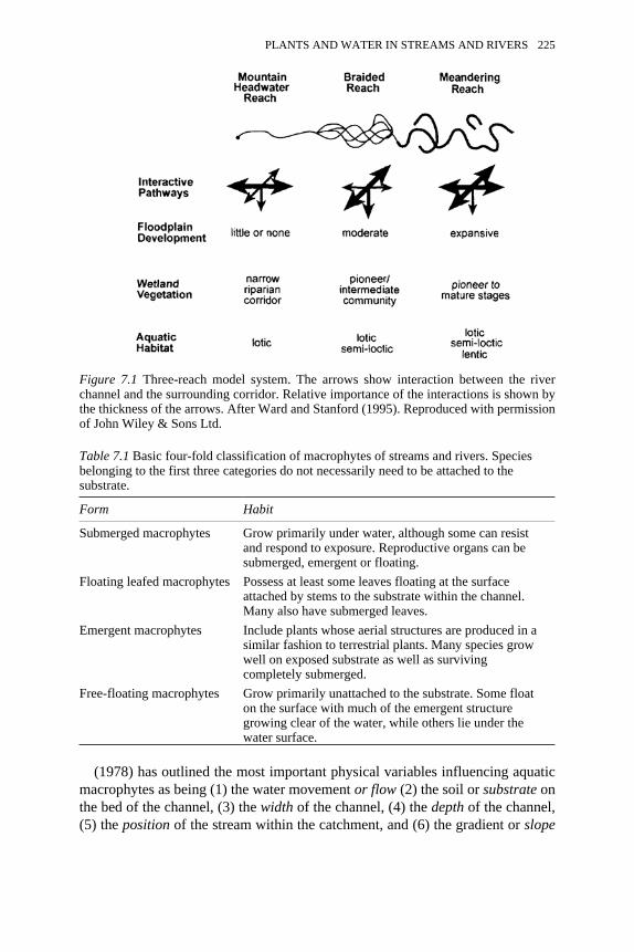
Table 7.1 Basic four-fold classification of macrophytes of streams and rivers. Speciesbelonging to the first three categories do not necessarily need to be attached to thesubstrate.
Form Habit
Submerged macrophytes Grow primarily under water, although some can resistand respond to exposure. Reproductive organs can besubmerged, emergent or floating.
Floating leafed macrophytes Possess at least some leaves floating at the surfaceattached by stems to the substrate within the channel.Many also have submerged leaves.
Emergent macrophytes Include plants whose aerial structures are produced in asimilar fashion to terrestrial plants. Many species growwell on exposed substrate as well as survivingcompletely submerged.
Free-floating macrophytes Grow primarily unattached to the substrate. Some floaton the surface with much of the emergent structuregrowing clear of the water, while others lie under thewater surface.
(1978) has outlined the most important physical variables influencing aquaticmacrophytes as being (1) the water movement or flow (2) the soil or substrate onthe bed of the channel, (3) the width of the channel, (4) the depth of the channel,(5) the position of the stream within the catchment, and (6) the gradient or slope
Figure 7.1 Three-reach model system. The arrows show interaction between the riverchannel and the surrounding corridor. Relative importance of the interactions is shown bythe thickness of the arrows. After Ward and Stanford (1995). Reproduced with permissionof John Wiley & Sons Ltd.
PLANTS AND WATER IN STREAMS AND RIVERS 225

of the channel. However, an inherent problem with analysing any of thesevariables is that some vary with each other and therefore cannot be considered astruly independent.
This chapter deals with plants and water in streams and rivers by dealing firstwith the movement of water in the channel, and examining the effect of plants onsuch water movement. A discussion of the effects of channel morphology andflow patterns on aquatic plants follows before consideration of the effects of (1)water quality on plants and (2) plants on water quality. The chapter concludeswith a discussion of the major effects of drought and flooding on the plants offluvial hydrosystems.
THE EFFECT OF PLANTS ON CHANNEL FLOW
In rivers, flow characteristics such as average and maximum depths, meanvelocities and secondary circulation patterns are governed by channel propertiesincluding cross-sectional shape, slope of the reach in question, and bank and bedmaterial properties, as well as the presence and form of instream and riparianvegetation (Bathurst, 1997). The water within a channel is subject to two mainforces: that of gravity, which causes flow downslope through a catchment, andfrictional forces leading to resistance against this downslope movement. In itssimplest form, a smooth and steeply sloping channel where frictional forces arelow and gravitational forces are high will have high flow velocities, while lowvelocities will be found in a low-gradient channel with high boundary roughness.
Mean water velocity in an open channel can be calculated using Manning’sequation:
(7.1)
where V is mean water velocity (m s−1), R is the hydraulic radius (ratio of wettedcross-sectional area to wetted perimeter), S is the channel slope (dimensionless),and n is a measure of channel roughness (dimensionless in this form of theequation—see Dingman, 1984: p. 113). Petts and Foster (1985) provide someexamples of Manning’s n but warn that estimation of empirical roughnesscoefficients is problematic because roughness is controlled not only byvegetation type and extent of cover but also by a number of other factors, whichinclude bed material size and bed form. In addition, these factors do not operateindividually but rather they interact in an often extremely complex manner.Wilson (1974) draws attention to the implications for estimating discharge,noting that, because n for natural streams is often about 0.035, an error in n of 0.001 gives an error in discharge of 3 percent. Smith et al. (1990) point out thatdifficulties in using the Manning equation arise in attempting to define thehydraulic radius of channels containing a significant volume of submergedvegetation, while Barnes (1967) attempted to produce a roughness classificationbased on photographs of channels of known roughness. Figure 7.2 shows the
226 ECO-HYDROLOGY
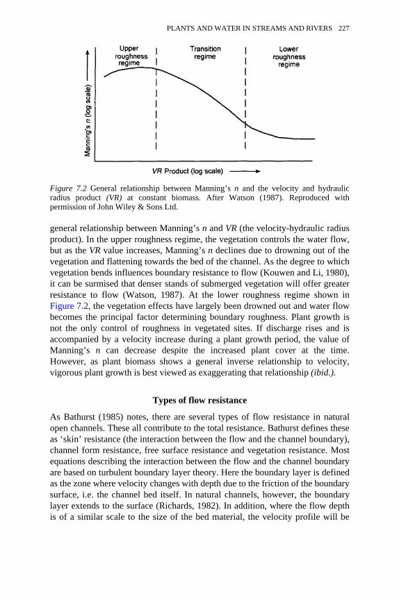
general relationship between Manning’s n and VR (the velocity-hydraulic radiusproduct). In the upper roughness regime, the vegetation controls the water flow,but as the VR value increases, Manning’s n declines due to drowning out of thevegetation and flattening towards the bed of the channel. As the degree to whichvegetation bends influences boundary resistance to flow (Kouwen and Li, 1980),it can be surmised that denser stands of submerged vegetation will offer greaterresistance to flow (Watson, 1987). At the lower roughness regime shown inFigure 7.2, the vegetation effects have largely been drowned out and water flowbecomes the principal factor determining boundary roughness. Plant growth isnot the only control of roughness in vegetated sites. If discharge rises and isaccompanied by a velocity increase during a plant growth period, the value ofManning’s n can decrease despite the increased plant cover at the time.However, as plant biomass shows a general inverse relationship to velocity,vigorous plant growth is best viewed as exaggerating that relationship (ibid.).
Types of flow resistance
As Bathurst (1985) notes, there are several types of flow resistance in naturalopen channels. These all contribute to the total resistance. Bathurst defines theseas ‘skin’ resistance (the interaction between the flow and the channel boundary),channel form resistance, free surface resistance and vegetation resistance. Mostequations describing the interaction between the flow and the channel boundaryare based on turbulent boundary layer theory. Here the boundary layer is definedas the zone where velocity changes with depth due to the friction of the boundarysurface, i.e. the channel bed itself. In natural channels, however, the boundarylayer extends to the surface (Richards, 1982). In addition, where the flow depthis of a similar scale to the size of the bed material, the velocity profile will be
Figure 7.2 General relationship between Manning’s n and the velocity and hydraulicradius product (VR) at constant biomass. After Watson (1987). Reproduced withpermission of John Wiley & Sons Ltd.
PLANTS AND WATER IN STREAMS AND RIVERS 227
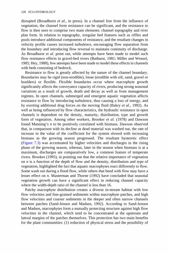
disrupted (Broadhurst et al., in press). In a channel free from the influence ofvegetation, the channel form resistance can be significant, and the resistance toflow is then seen to comprise two main elements: channel topography and riverplan form. In relation to topography, irregular bed features such as riffles andpools introduce additional components of resistance, and the resultant changes invelocity profile causes increased turbulence, encouraging flow separation fromthe boundary and introducing flow reversal to maintain continuity of discharge.As Broadhurst et al. point out, while attempts have been made to model suchflow resistance effects in gravel-bed rivers (Bathurst, 1981; Miller and Wenzel,1985; Hey, 1988), few attempts have been made to model these effects in channelswith beds consisting of bedrock.
Resistance to flow is greatly affected by the nature of the channel boundary.Boundaries may be rigid (non-erodible), loose (erodible with silt, sand, gravel orboulders) or flexible. Flexible boundaries occur where macrophyte growthsignificantly affects the conveyance capacity of rivers, producing strong seasonalvariations as a result of growth, death and decay as well as from managementregimes. In open channels, submerged and emergent aquatic vegetation affectsresistance to flow by introducing turbulence, thus causing a loss of energy, andby exerting additional drag forces on the moving fluid (Bakry et al., 1992). Aswell as being influenced by flow characteristics, the hydraulic resistance in openchannels is dependent on the density, maturity, distribution, type and growthform of vegetation. Among other workers, Brooker et al. (1978) and Dawsonfound Manning’s n to be positively correlated with biomass. Dawson observedthat, in comparison with its decline as dead material was washed out, the rate ofincrease in the value of the coefficient for the system slowed with increasingbiomass as the growing season progressed. The resultant hysteretic effect(Figure 7.3) was accentuated by higher velocities and discharges in the risingphase of the growing season, whereas, later in the season when biomass is at amaximum, discharges are comparatively low, a common feature of temperaterivers. Brookes (1995), in pointing out that the relative importance of vegetationon n is a function of the depth of flow and the density, distribution and type ofvegetation, highlighted the fact that aquatic macrophytes react differently to flow.Some wash out during a flood flow, while others that bend with flow may have alesser effect on n. Masterman and Thorne (1992) have concluded that seasonalvegetation growth can have a significant effect in reducing channel capacitywhere the width-depth ratio of the channel is less than 16.
Patchy macrophyte distribution creates a diverse in-stream habitat with lowflow velocities and fine-grained sediments within macrophyte patches, and highflow velocities and coarser sediments in the deeper and often narrow channelsbetween patches (Sand-Jensen and Madsen, 1992). According to Sand-Jensenand Madsen, macrophytes form a mutually protecting structure against high flowvelocities in the channel, which tend to be concentrated at the upstream andlateral margins of the patches themselves. This protection has two main benefitsfor the plant communities: (1) reduction of physical stress and the possibility of
228 ECO-HYDROLOGY
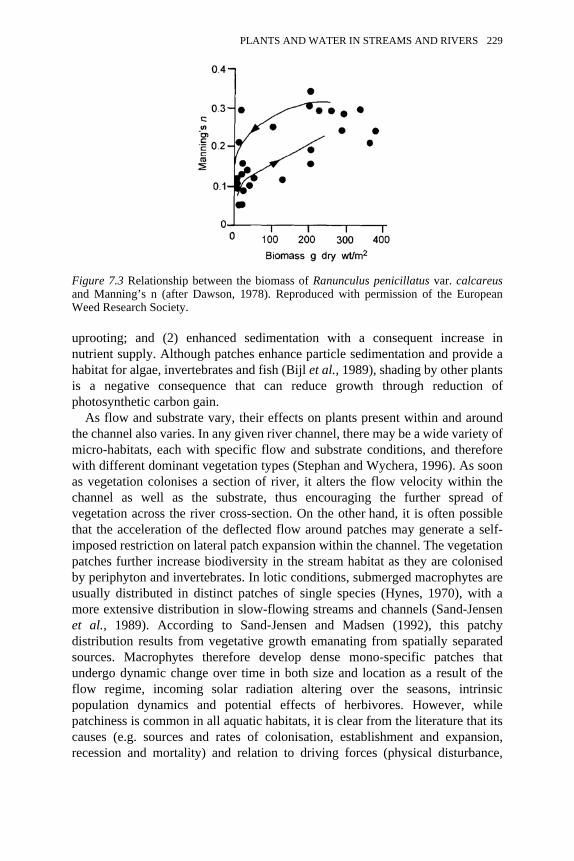
uprooting; and (2) enhanced sedimentation with a consequent increase innutrient supply. Although patches enhance particle sedimentation and provide ahabitat for algae, invertebrates and fish (Bijl et al., 1989), shading by other plantsis a negative consequence that can reduce growth through reduction ofphotosynthetic carbon gain.
As flow and substrate vary, their effects on plants present within and aroundthe channel also varies. In any given river channel, there may be a wide variety ofmicro-habitats, each with specific flow and substrate conditions, and thereforewith different dominant vegetation types (Stephan and Wychera, 1996). As soonas vegetation colonises a section of river, it alters the flow velocity within thechannel as well as the substrate, thus encouraging the further spread ofvegetation across the river cross-section. On the other hand, it is often possiblethat the acceleration of the deflected flow around patches may generate a self-imposed restriction on lateral patch expansion within the channel. The vegetationpatches further increase biodiversity in the stream habitat as they are colonisedby periphyton and invertebrates. In lotic conditions, submerged macrophytes areusually distributed in distinct patches of single species (Hynes, 1970), with amore extensive distribution in slow-flowing streams and channels (Sand-Jensenet al., 1989). According to Sand-Jensen and Madsen (1992), this patchydistribution results from vegetative growth emanating from spatially separatedsources. Macrophytes therefore develop dense mono-specific patches thatundergo dynamic change over time in both size and location as a result of theflow regime, incoming solar radiation altering over the seasons, intrinsicpopulation dynamics and potential effects of herbivores. However, whilepatchiness is common in all aquatic habitats, it is clear from the literature that itscauses (e.g. sources and rates of colonisation, establishment and expansion,recession and mortality) and relation to driving forces (physical disturbance,
Figure 7.3 Relationship between the biomass of Ranunculus penicillatus var. calcareusand Manning’s n (after Dawson, 1978). Reproduced with permission of the EuropeanWeed Research Society.
PLANTS AND WATER IN STREAMS AND RIVERS 229
environmental gradients, biotic influences) have only been studied occasionally.Mono-specific patches are often typical of extreme site conditions (Grime, 1979).
While the distribution of aquatic macrophytes is aligned along the twoprincipal environmental gradients of water depth and substrate type (Day et al.,1988), competition is a third factor that partly controls macrophyte distributions(Wilson and Keddy 1986; 1991; Grace, 1987). The first two gradients determinethe extent of a species’ occurrence, which in turn affects the outcome ofcompetition (Gopal and Goel, 1993). A pattern of increasing flow rate (the resultof shear stress at the surface and the viscous nature of the water in the streamitself) can be seen as one moves away from the submerged vegetation surfaceand into what Losee and Wetzel (1993) have termed the hydrodynamic boundarylayer.
The relationships between flow rates, the structure and species dominance ofthe submerged plant community are complex. In-stream flow rates are affectedby the interaction of the flowing water with the entire plant community. Theeffects for an individual plant as a member of a submerged community includenot only reduced flow rates but also protection from shear under rapid flow rates.Rapid fluctuations occur in littoral flow rates, and this means that the submergedplant boundary layer may be unstable (ibid.). Plants bend in the current anddeflect flow over and around the vegetation. As a consequence of the pressuredrag of the vegetation, flow is accelerated around the macrophyte patches (Sand-Jensen and Mebus, 1996), and the resultant energy is then dissipated in thepronounced vortices downstream of the patches. Results obtained by Newall(1995) show that the presence of aquatic plants provides very differentenvironments from those found in open flow situations. While downstream flowsare likely to be affected by in-stream stands of macrophytes, how far the effectsextend downstream depends on the structure and species content of themacrophyte stand and has direct implications for the habitat diversity of thesemicro-flow environments. The potential for habitat partitioning in aquaticmacrophyte communities is great as these environments are often heterogeneouswith respect to flow velocity, depth and sediment texture (French and Chambers,1996). Supporting this is the fact that greater numbers of macroinvertebrates arefound in macrophyte patches than anywhere else in the aquatic environment(Marshall and Westlake, 1978). However, while habitat partitioning has beenextensively studied in terrestrial plant communities, less attention has been paidto the aquatic environment.
Macrophyte stands shelter other macrophytes from scouring currents, therebyfacilitating recruitment and increasing survival rates. Figure 7.4 summarises themain roles that rooted macrophytes play in regulating the physical conditions andbiological structure of lowland streams. As different plant species have differenteffects on flow turbulence (Watts and Watts, 1990), it can be seen how stands ofaquatic macrophytes provide refugia from the main body of flow at varyingstages in the life-cycle for biota such as invertebrates and fish. While current andlight are the major controlling factors of the ‘micro-environment’ (Dodds, 1991)
230 ECO-HYDROLOGY
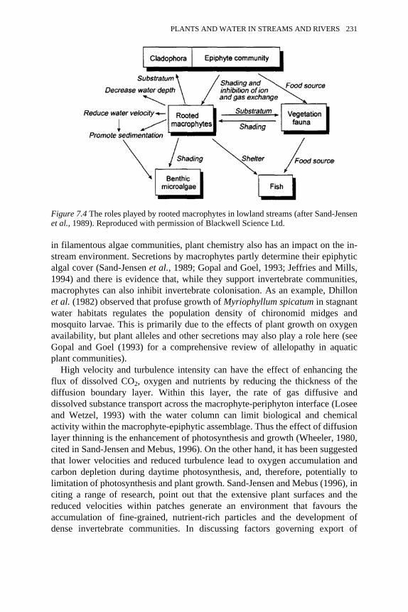
in filamentous algae communities, plant chemistry also has an impact on the in-stream environment. Secretions by macrophytes partly determine their epiphyticalgal cover (Sand-Jensen et al., 1989; Gopal and Goel, 1993; Jeffries and Mills,1994) and there is evidence that, while they support invertebrate communities,macrophytes can also inhibit invertebrate colonisation. As an example, Dhillonet al. (1982) observed that profuse growth of Myriophyllum spicatum in stagnantwater habitats regulates the population density of chironomid midges andmosquito larvae. This is primarily due to the effects of plant growth on oxygenavailability, but plant alleles and other secretions may also play a role here (seeGopal and Goel (1993) for a comprehensive review of allelopathy in aquaticplant communities).
High velocity and turbulence intensity can have the effect of enhancing theflux of dissolved CO2, oxygen and nutrients by reducing the thickness of thediffusion boundary layer. Within this layer, the rate of gas diffusive anddissolved substance transport across the macrophyte-periphyton interface (Loseeand Wetzel, 1993) with the water column can limit biological and chemicalactivity within the macrophyte-epiphytic assemblage. Thus the effect of diffusionlayer thinning is the enhancement of photosynthesis and growth (Wheeler, 1980,cited in Sand-Jensen and Mebus, 1996). On the other hand, it has been suggestedthat lower velocities and reduced turbulence lead to oxygen accumulation andcarbon depletion during daytime photosynthesis, and, therefore, potentially tolimitation of photosynthesis and plant growth. Sand-Jensen and Mebus (1996), inciting a range of research, point out that the extensive plant surfaces and thereduced velocities within patches generate an environment that favours theaccumulation of fine-grained, nutrient-rich particles and the development ofdense invertebrate communities. In discussing factors governing export of
Figure 7.4 The roles played by rooted macrophytes in lowland streams (after Sand-Jensenet al., 1989). Reproduced with permission of Blackwell Science Ltd.
PLANTS AND WATER IN STREAMS AND RIVERS 231
macrophyte detritus from patches, Carpenter and Lodge (1986) also suggestedthat macrophyte beds act as sieving mechanisms retaining particulate detritus (cf.Figure 7.4). Within streams, the processes of sedimentation and colonisation byvegetation typically occurs at low flows, followed by wash-out as discharge rises(Dawson, 1976).
Submerged macrophytes therefore form permanent biotic communities inshallow temperate lowland streams. Stephan and Wychera (1996) summarise themain effects of colonisation of a river section by macrophytes as follows:
• General reduction of cross-sectional flow velocity.• Increase of flow velocity in parts of the cross-sectional area not occupied by
vegetation.• Decrease of flow velocity in the close vicinity of the macrophyte stand.• Generally increased sedimentation in the cross-sectional area as a result of
reduced flow velocity.
There are five main mechanisms by which the vegetation of streams and riversexerts control over fluvial processes: (1) provision of flow resistance, (2)provision of bank strength, (3) influence on bar sedimentation and erosion, (4)formation of log jams, and (5) effect on concave-bank bench deposition (Hicken,1984; Gregory, 1992; Gurnell et al., 1995). Out of the channel itself, the mainhydrological effects of rooted vegetation include impacts on bank water tablelevels and on influent/effluent bank seepage. Besides the living biomassproduced by aquatic macrophytes, dead biomass of varying origin, transportedby the stream’s waters, is also of great ecological importance, being a substratefor many heterotrophs. Moreover, larger woody debris, especially tree trunksfalling into the channel, provides habitat for colonisation by aquatic algae,bryophytes and higher plants, as well as invertebrates and fungi, thus increasingthe overall biodiversity of the channel.
Perhaps the most dramatic way in which plants directly affect the flow ofwater in streams and rivers is in the form of woody debris dams. These impedelow to medium flows, producing a step-pool sequence in smaller rivers, and avariety of plunge-, marginal- and backwater-pool habitats in medium-sized rivers(Triska and Cromack, 1980; Bisson et al., 1987). This is advantageous for thebiota through the maintenance of pool areas, as well as causing local variationsin bank hydrology (Gurnell and Gregory, 1987). The attenuation of low tomedium flows and the enhanced interaction with the alluvial aquifer may havevery important impacts on water quality as well as on the hydrology of the riversystem (Gurnell, 1997). Such dams also dissipate the river’s energy at specificlocations along the long profile, resulting in the development of plunge pools andlocal sorting of bed material in small streams and the development of marginalscour zones in larger rivers.
232 ECO-HYDROLOGY
THE EFFECTS OF CHANNEL MORPHOLOGY ANDFLOW PATTERNS ON AQUATIC PLANTS
While plants alter the flow pattern of a stream, they are also themselvessignificantly affected by alterations in flow regime and flow pattern. Indeed,water movement is perhaps the most important factor affecting plants and theirdistribution in streams and rivers. While Gilvear and Bravard (1996) state that aknowledge of river flow hydraulics is essential for an understanding of rivergeomorphology, a knowledge of flow hydraulics is also important for anunderstanding of plant growth and distribution, as hydraulic processes operatingwithin the channel determine the nature of the aquatic biotopes (the physicalenvironment of the biotic community) found therein. As well as affecting plantsdirectly, flow also has an indirect effect by virtue of its influence on the bed ofthe channel (Haslam, 1978). Haslam divided the flow conditions affecting riverplants into five main categories— negligible flow; slow flow, where trailingplants hardly move; moderate flow, where trailing plants clearly move and thesurface is disturbed; fast flow, where the vegetation moves vigorously and thesurface is markedly disturbed; and, finally, spate flow. The spate flow typicallycauses the most damage to aquatic plant communities. A combination ofchanging channel morphology and flow patterns is well expressed in thedownstream direction influencing plant distribution. Distribution histogramsproduced by Haslam (Figure 7.5) show species to have ranges of tolerance,including ranges in which they grow well, ranges in which they grow less well orless frequently and ranges where they are absent altogether. It should be borne inmind, however, that channels are seldom uniform (except in channelised cases)and that these patterns may be complicated due to habitat variations within thesame reach.
Plants are affected by flow at all stages of their life-cycle. Hydrochory, i.e.dispersal by water, is one of the major dispersal mechanisms for plants alongriver corridors, as both seeds and vegetative propagules are transported anddispersed by water. While the importance of hydrochory in dispersing plantpropagules of single species along watercourses is recognised (e.g. Schneiderand Sharitz, 1988), its importance in structuring whole plant communities alongrivers is not well understood (Nilsson et al., 1991; Johansson and Nilsson, 1993).
Remarks on invasive species
Some undesirable exotic species spread along rivers because of easy movementof their diaspores by water (Malanson, 1993; Pyšek and Prach, 1993; Pyšek,1994) and frequent occurrence of disturbed micro-habitats suitable for theirestablishment. In temperate Europe, species such as Fallopia japonica,Impatiens glandulifera (Figure 7.6) and Heracleum mantegazzianum are amongthe most aggressive colonisers of riverside habitats, having distinct competitive
PLANTS AND WATER IN STREAMS AND RIVERS 233
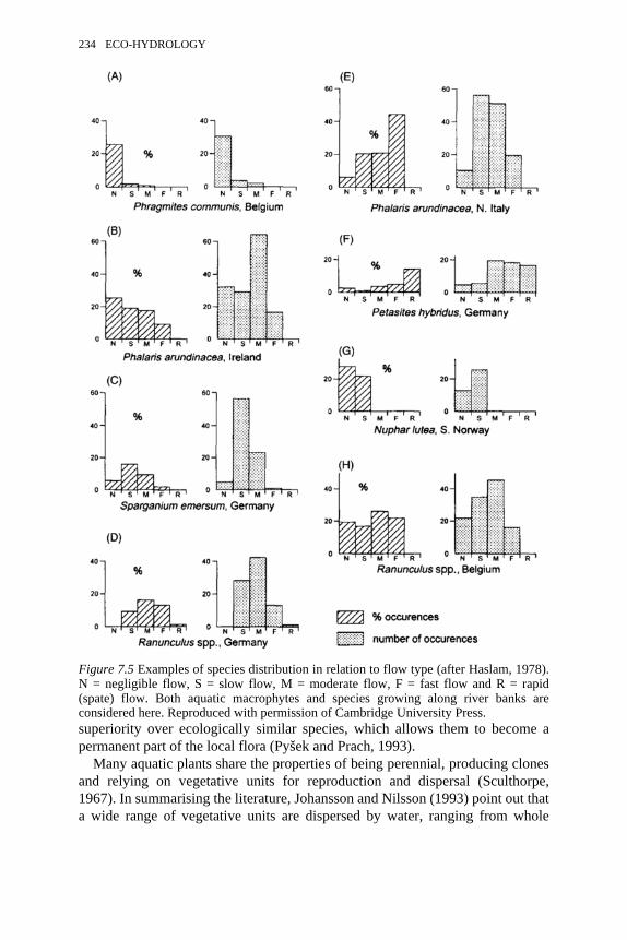
superiority over ecologically similar species, which allows them to become apermanent part of the local flora (Pyšek and Prach, 1993).
Many aquatic plants share the properties of being perennial, producing clonesand relying on vegetative units for reproduction and dispersal (Sculthorpe,1967). In summarising the literature, Johansson and Nilsson (1993) point out thata wide range of vegetative units are dispersed by water, ranging from whole
Figure 7.5 Examples of species distribution in relation to flow type (after Haslam, 1978).N = negligible flow, S = slow flow, M = moderate flow, F = fast flow and R = rapid(spate) flow. Both aquatic macrophytes and species growing along river banks areconsidered here. Reproduced with permission of Cambridge University Press.
234 ECO-HYDROLOGY
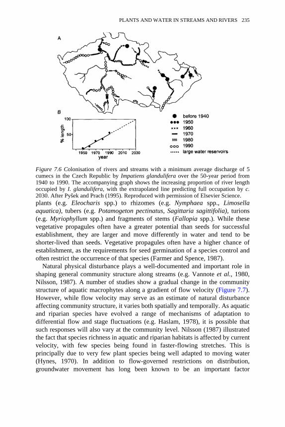
plants (e.g. Eleocharis spp.) to rhizomes (e.g. Nymphaea spp., Limosellaaquatica), tubers (e.g. Potamogeton pectinatus, Sagittaria sagittifolia), turions(e.g. Myriophyllum spp.) and fragments of stems (Fallopia spp.). While thesevegetative propagules often have a greater potential than seeds for successfulestablishment, they are larger and move differently in water and tend to beshorter-lived than seeds. Vegetative propagules often have a higher chance ofestablishment, as the requirements for seed germination of a species control andoften restrict the occurrence of that species (Farmer and Spence, 1987).
Natural physical disturbance plays a well-documented and important role inshaping general community structure along streams (e.g. Vannote et al., 1980,Nilsson, 1987). A number of studies show a gradual change in the communitystructure of aquatic macrophytes along a gradient of flow velocity (Figure 7.7).However, while flow velocity may serve as an estimate of natural disturbanceaffecting community structure, it varies both spatially and temporally. As aquaticand riparian species have evolved a range of mechanisms of adaptation todifferential flow and stage fluctuations (e.g. Haslam, 1978), it is possible thatsuch responses will also vary at the community level. Nilsson (1987) illustratedthe fact that species richness in aquatic and riparian habitats is affected by currentvelocity, with few species being found in faster-flowing stretches. This isprincipally due to very few plant species being well adapted to moving water(Hynes, 1970). In addition to flow-governed restrictions on distribution,groundwater movement has long been known to be an important factor
Figure 7.6 Colonisation of rivers and streams with a minimum average discharge of 5cumecs in the Czech Republic by Impatiens glandulifera over the 50-year period from1940 to 1990. The accompanying graph shows the increasing proportion of river lengthoccupied by I. glandulifera, with the extrapolated line predicting full occupation by c.2030. After Pyšek and Prach (1995). Reproduced with permission of Elsevier Science.
PLANTS AND WATER IN STREAMS AND RIVERS 235
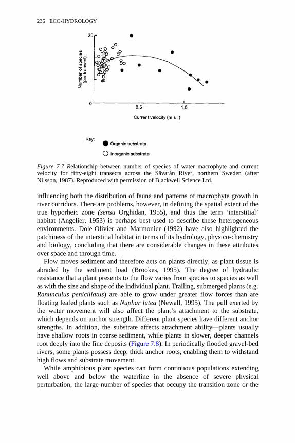
influencing both the distribution of fauna and patterns of macrophyte growth inriver corridors. There are problems, however, in defining the spatial extent of thetrue hyporheic zone (sensu Orghidan, 1955), and thus the term ‘interstitial’habitat (Angelier, 1953) is perhaps best used to describe these heterogeneousenvironments. Dole-Olivier and Marmonier (1992) have also highlighted thepatchiness of the interstitial habitat in terms of its hydrology, physico-chemistryand biology, concluding that there are considerable changes in these attributesover space and through time.
Flow moves sediment and therefore acts on plants directly, as plant tissue isabraded by the sediment load (Brookes, 1995). The degree of hydraulicresistance that a plant presents to the flow varies from species to species as wellas with the size and shape of the individual plant. Trailing, submerged plants (e.g.Ranunculus penicillatus) are able to grow under greater flow forces than arefloating leafed plants such as Nuphar lutea (Newall, 1995). The pull exerted bythe water movement will also affect the plant’s attachment to the substrate,which depends on anchor strength. Different plant species have different anchorstrengths. In addition, the substrate affects attachment ability—plants usuallyhave shallow roots in coarse sediment, while plants in slower, deeper channelsroot deeply into the fine deposits (Figure 7.8). In periodically flooded gravel-bedrivers, some plants possess deep, thick anchor roots, enabling them to withstandhigh flows and substrate movement.
While amphibious plant species can form continuous populations extendingwell above and below the waterline in the absence of severe physicalperturbation, the large number of species that occupy the transition zone or the
Figure 7.7 Relationship between number of species of water macrophyte and currentvelocity for fifty-eight transects across the Sävarån River, northern Sweden (afterNilsson, 1987). Reproduced with permission of Blackwell Science Ltd.
236 ECO-HYDROLOGY
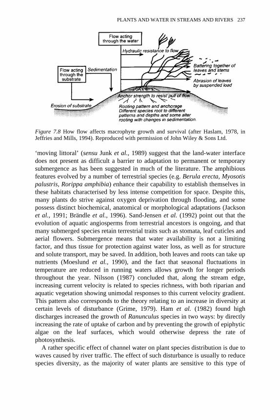
‘moving littoral’ (sensu Junk et al., 1989) suggest that the land-water interfacedoes not present as difficult a barrier to adaptation to permanent or temporarysubmergence as has been suggested in much of the literature. The amphibiousfeatures evolved by a number of terrestrial species (e.g. Berula erecta, Myosotispalustris, Rorippa amphibia) enhance their capability to establish themselves inthese habitats characterised by less intense competition for space. Despite this,many plants do strive against oxygen deprivation through flooding, and somepossess distinct biochemical, anatomical or morphological adaptations (Jacksonet al., 1991; Brändle et al., 1996). Sand-Jensen et al. (1992) point out that theevolution of aquatic angiosperms from terrestrial ancestors is ongoing, and thatmany submerged species retain terrestrial traits such as stomata, leaf cuticles andaerial flowers. Submergence means that water availability is not a limitingfactor, and thus tissue for protection against water loss, as well as for structureand solute transport, may be saved. In addition, both leaves and roots can take upnutrients (Moeslund et al., 1990), and the fact that seasonal fluctuations intemperature are reduced in running waters allows growth for longer periodsthroughout the year. Nilsson (1987) concluded that, along the stream edge,increasing current velocity is related to species richness, with both riparian andaquatic vegetation showing unimodal responses to this current velocity gradient.This pattern also corresponds to the theory relating to an increase in diversity atcertain levels of disturbance (Grime, 1979). Ham et al. (1982) found highdischarges increased the growth of Ranunculus species in two ways: by directlyincreasing the rate of uptake of carbon and by preventing the growth of epiphyticalgae on the leaf surfaces, which would otherwise depress the rate ofphotosynthesis.
A rather specific effect of channel water on plant species distribution is due towaves caused by river traffic. The effect of such disturbance is usually to reducespecies diversity, as the majority of water plants are sensitive to this type of
Figure 7.8 How flow affects macrophyte growth and survival (after Haslam, 1978, inJeffries and Mills, 1994). Reproduced with permission of John Wiley & Sons Ltd.
PLANTS AND WATER IN STREAMS AND RIVERS 237
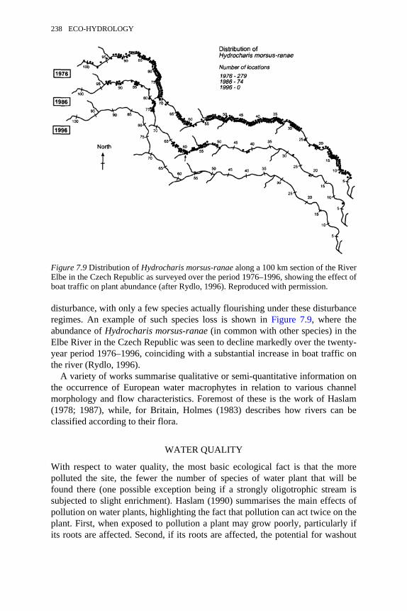
disturbance, with only a few species actually flourishing under these disturbanceregimes. An example of such species loss is shown in Figure 7.9, where theabundance of Hydrocharis morsus-ranae (in common with other species) in theElbe River in the Czech Republic was seen to decline markedly over the twenty-year period 1976–1996, coinciding with a substantial increase in boat traffic onthe river (Rydlo, 1996).
A variety of works summarise qualitative or semi-quantitative information onthe occurrence of European water macrophytes in relation to various channelmorphology and flow characteristics. Foremost of these is the work of Haslam(1978; 1987), while, for Britain, Holmes (1983) describes how rivers can beclassified according to their flora.
WATER QUALITY
With respect to water quality, the most basic ecological fact is that the morepolluted the site, the fewer the number of species of water plant that will befound there (one possible exception being if a strongly oligotrophic stream issubjected to slight enrichment). Haslam (1990) summarises the main effects ofpollution on water plants, highlighting the fact that pollution can act twice on theplant. First, when exposed to pollution a plant may grow poorly, particularly ifits roots are affected. Second, if its roots are affected, the potential for washout
Figure 7.9 Distribution of Hydrocharis morsus-ranae along a 100 km section of the RiverElbe in the Czech Republic as surveyed over the period 1976–1996, showing the effect ofboat traffic on plant abundance (after Rydlo, 1996). Reproduced with permission.
238 ECO-HYDROLOGY
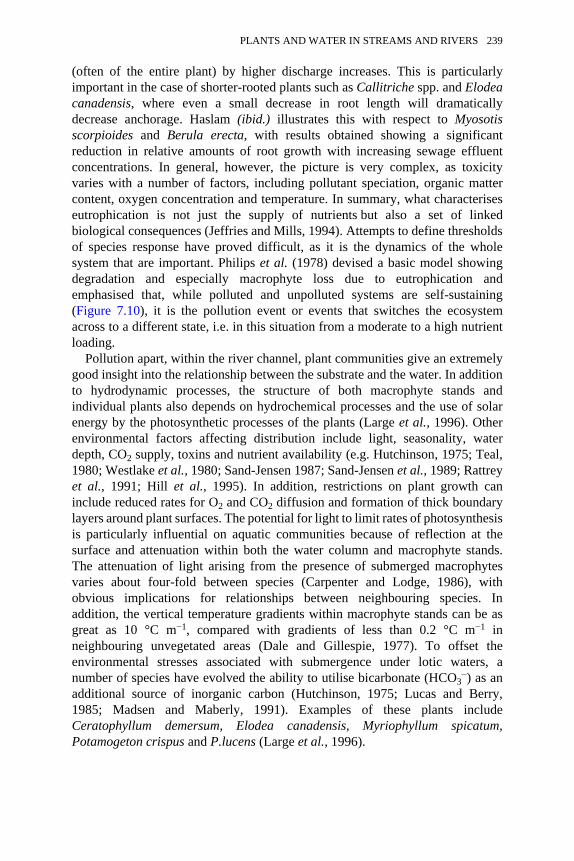
(often of the entire plant) by higher discharge increases. This is particularlyimportant in the case of shorter-rooted plants such as Callitriche spp. and Elodeacanadensis, where even a small decrease in root length will dramaticallydecrease anchorage. Haslam (ibid.) illustrates this with respect to Myosotisscorpioides and Berula erecta, with results obtained showing a significantreduction in relative amounts of root growth with increasing sewage effluentconcentrations. In general, however, the picture is very complex, as toxicityvaries with a number of factors, including pollutant speciation, organic mattercontent, oxygen concentration and temperature. In summary, what characteriseseutrophication is not just the supply of nutrients but also a set of linkedbiological consequences (Jeffries and Mills, 1994). Attempts to define thresholdsof species response have proved difficult, as it is the dynamics of the wholesystem that are important. Philips et al. (1978) devised a basic model showingdegradation and especially macrophyte loss due to eutrophication andemphasised that, while polluted and unpolluted systems are self-sustaining(Figure 7.10), it is the pollution event or events that switches the ecosystemacross to a different state, i.e. in this situation from a moderate to a high nutrientloading.
Pollution apart, within the river channel, plant communities give an extremelygood insight into the relationship between the substrate and the water. In additionto hydrodynamic processes, the structure of both macrophyte stands andindividual plants also depends on hydrochemical processes and the use of solarenergy by the photosynthetic processes of the plants (Large et al., 1996). Otherenvironmental factors affecting distribution include light, seasonality, waterdepth, CO2 supply, toxins and nutrient availability (e.g. Hutchinson, 1975; Teal,1980; Westlake et al., 1980; Sand-Jensen 1987; Sand-Jensen et al., 1989; Rattreyet al., 1991; Hill et al., 1995). In addition, restrictions on plant growth caninclude reduced rates for O2 and CO2 diffusion and formation of thick boundarylayers around plant surfaces. The potential for light to limit rates of photosynthesisis particularly influential on aquatic communities because of reflection at thesurface and attenuation within both the water column and macrophyte stands.The attenuation of light arising from the presence of submerged macrophytesvaries about four-fold between species (Carpenter and Lodge, 1986), withobvious implications for relationships between neighbouring species. Inaddition, the vertical temperature gradients within macrophyte stands can be asgreat as 10 °C m−1, compared with gradients of less than 0.2 °C m−1 inneighbouring unvegetated areas (Dale and Gillespie, 1977). To offset theenvironmental stresses associated with submergence under lotic waters, anumber of species have evolved the ability to utilise bicarbonate (HCO3
−) as anadditional source of inorganic carbon (Hutchinson, 1975; Lucas and Berry,1985; Madsen and Maberly, 1991). Examples of these plants includeCeratophyllum demersum, Elodea canadensis, Myriophyllum spicatum,Potamogeton crispus and P.lucens (Large et al., 1996).
PLANTS AND WATER IN STREAMS AND RIVERS 239
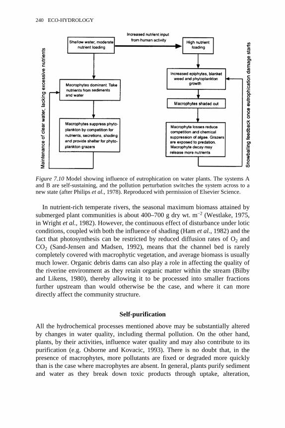
In nutrient-rich temperate rivers, the seasonal maximum biomass attained bysubmerged plant communities is about 400–700 g dry wt. m−2 (Westlake, 1975,in Wright et al., 1982). However, the continuous effect of disturbance under loticconditions, coupled with both the influence of shading (Ham et al., 1982) and thefact that photosynthesis can be restricted by reduced diffusion rates of O2 andCO2 (Sand-Jensen and Madsen, 1992), means that the channel bed is rarelycompletely covered with macrophytic vegetation, and average biomass is usuallymuch lower. Organic debris dams can also play a role in affecting the quality ofthe riverine environment as they retain organic matter within the stream (Bilbyand Likens, 1980), thereby allowing it to be processed into smaller fractionsfurther upstream than would otherwise be the case, and where it can moredirectly affect the community structure.
Self-purification
All the hydrochemical processes mentioned above may be substantially alteredby changes in water quality, including thermal pollution. On the other hand,plants, by their activities, influence water quality and may also contribute to itspurification (e.g. Osborne and Kovacic, 1993). There is no doubt that, in thepresence of macrophytes, more pollutants are fixed or degraded more quicklythan is the case where macrophytes are absent. In general, plants purify sedimentand water as they break down toxic products through uptake, alteration,
Figure 7.10 Model showing influence of eutrophication on water plants. The systems Aand B are self-sustaining, and the pollution perturbation switches the system across to anew state (after Philips et al., 1978). Reproduced with permission of Elsevier Science.
240 ECO-HYDROLOGY
production of root exudates and the influence of microphytic micro-organisms.In addition, Haslam (1987) mentions that the micro-organisms Escherichia coli,Salmonella and Enterococcus are eliminated to different degrees by plant speciessuch as Mentha aquatica, Alisma plantago-aquatica, Iris pseudacorus,Juncuseffusus, Scirpus lacustris and Phragmites australis, principally throughallelopathic mechanisms. This self-purification ability is particularly evident inriparian areas and wetlands contained within the river corridor, and it hasimportant implications in relation to water quality management andimprovement. Numerous publications have addressed this in recent years.Riparian zones have been described as the ‘kidneys’ of the water landscape(Fennessy, 1993) and, via the action of the vegetation, can act as nutrient sinks,thereby protecting surface and subsurface waters from enrichment byagricultural nutrients and other sources of pollution. This is in addition to anumber of other functions that they fulfil in the riparian landscape (Large andPetts, 1994). The ability of plants to remove nitrogen is primarily a function ofplant uptake and denitrification (e.g. Lowrance et al., 1985; Haycock and Pinay,1993; Muscutt et al., 1993; Vought et al., 1994). Of the two, denitrification is themost dominant and longer-lasting removal process (Fennessy, 1993). Plantcommunities therefore carry out a number of important functions: they take upnutrients directly, binding them in biomass and freeing exchange sites in thesoils, while their litter provides habitats for microbe colonisation and, along withroot exudates, forms the primary source of organic carbon used in denitrification.In addition, it has been stated that the presence of vegetation significantlyincreases the amount of oxygen in the soil through the formation of oxidisedrhizospheres (ibid.), although other workers question the importance of thisprocess (see also Chapter 5). Questions still to be answered effectively includewhat constitutes the optimal width for a vegetated buffer strip, and what speciesare most efficient in taking up nutrients (Large and Petts, 1994). Decompositionprocesses and nutrient release in freshwater systems have a strong seasonality(Polunin, 1982; 1984), raising concerns as to what are the seasonal variations ineffectiveness. Furthermore, nutrient release may occur as a result of senescence(Large and Petts 1994) and decomposition of the vegetation in situ. Thus,problems may arise when the buffer strip becomes saturated with nutrients(Large and Petts, 1992). In summary, the plants of riparian habitats can beviewed as bidirectional buffers—while they buffer the effects of surface andsubsurface runoff on river waters, they also buffer the effects of river flooding onadjacent areas within the river corridor. These effects vary on a temporal basisdue to seasonal variation in water flows in rivers themselves.
DROUGHT AND FLOOD
While individual river plants are influenced by both ‘normal’ and extreme flows,extreme events are often critical in determining ecosystem composition andfunctioning (Haslam 1978). Community composition is determined by the
PLANTS AND WATER IN STREAMS AND RIVERS 241
presence or absence of flooding and its duration and frequency. Haslam (ibid.)suggests that drought flows can be important if they substantially alter turbulenceor silting, but they generally have a more localised effect than flooding. He may,however, have underestimated the effects of drought. For example, depletedgroundwater levels in chalk catchments in southern England during the late 1980sand the 1990s dramatically reduced flows in some channels and is likely to havehad a profound effect on plant distributions. Intensified research efforts will benecessary to ascertain and quantify these effects. Flooding, on the other hand,constitutes an important environmental factor that influences plant compositionand plant growth in many parts of the world. While gradients in stream size,water depth, current velocity, substrate composition and standing crop allproduce predictable patterns in riverbank vegetation (Day et al., 1988; Nilssonand Grelsson, 1989; Nilsson et al., 1989) in systems unmodified by humans,disturbance via flooding constitutes a key factor in the distribution of plantspecies and the intensity of their production. A disturbance here is defined as asignificant change from the normal pattern in an ecological system (Forman andGodron, 1986, Pickett and White, 1985, Resh et al., 1988). In fluvialhydrosystems, such disturbance can be direct (e.g. inundation, desiccation,erosion, siltation, bar formation) or indirect (e.g. alterations to the hydrochemicalgradient) and can follow on from other changes in the ecosystem (e.g. redirectionof succession sequences). Any plant can be damaged by extreme flow events,although different species are likely to be affected in different ways. Plants thatgrow on soft sediments are particularly vulnerable to scour and damage.Recovery of these species depends on the presence of plant fragments and isenhanced if roots or rhizomes remain in situ. Haslam (1978) provides a goodsummary of the susceptibility of individual species to storm damage and concludesthat plant vigour has an additional bearing on resistance to damage from extremeflows.
The flood pulse
As Junk et al. (1989) have concluded, the principal driving force for theexistence, productivity and interactions of the major biota in river-floodplainsystems is the flood pulse. They define the flood pulse as a ‘batch’ process, asdistinct from the continuous processes in flowing water environments consideredin the ‘River continuum concept’ (Vannote et al., 1980), which hypothesises thata continuous gradient of physical conditions exists from headwater to mouth in astream system. A flood event has two types of effect on the mosaic pattern of thefluvial unit. First, it can, by inundating the unit, affect the communities withoutaltering the biotope. Alternatively, the flood can transform the biotope througherosion and deposition of alluvium, provoking a marked change in the speciescomposition of the plant communities. This has been described as the ‘biologicalresetting’ of the system. Besides importing nutrients, inundating floods carryorganic debris, which accumulates locally in the form of litter throughout the
242 ECO-HYDROLOGY
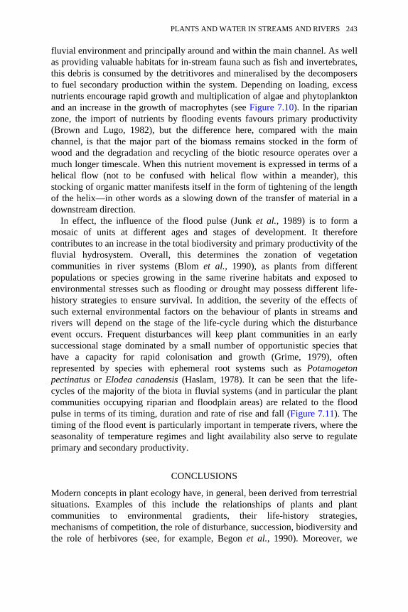
fluvial environment and principally around and within the main channel. As wellas providing valuable habitats for in-stream fauna such as fish and invertebrates,this debris is consumed by the detritivores and mineralised by the decomposersto fuel secondary production within the system. Depending on loading, excessnutrients encourage rapid growth and multiplication of algae and phytoplanktonand an increase in the growth of macrophytes (see Figure 7.10). In the riparianzone, the import of nutrients by flooding events favours primary productivity(Brown and Lugo, 1982), but the difference here, compared with the mainchannel, is that the major part of the biomass remains stocked in the form ofwood and the degradation and recycling of the biotic resource operates over amuch longer timescale. When this nutrient movement is expressed in terms of ahelical flow (not to be confused with helical flow within a meander), thisstocking of organic matter manifests itself in the form of tightening of the lengthof the helix—in other words as a slowing down of the transfer of material in adownstream direction.
In effect, the influence of the flood pulse (Junk et al., 1989) is to form amosaic of units at different ages and stages of development. It thereforecontributes to an increase in the total biodiversity and primary productivity of thefluvial hydrosystem. Overall, this determines the zonation of vegetationcommunities in river systems (Blom et al., 1990), as plants from differentpopulations or species growing in the same riverine habitats and exposed toenvironmental stresses such as flooding or drought may possess different life-history strategies to ensure survival. In addition, the severity of the effects ofsuch external environmental factors on the behaviour of plants in streams andrivers will depend on the stage of the life-cycle during which the disturbanceevent occurs. Frequent disturbances will keep plant communities in an earlysuccessional stage dominated by a small number of opportunistic species thathave a capacity for rapid colonisation and growth (Grime, 1979), oftenrepresented by species with ephemeral root systems such as Potamogetonpectinatus or Elodea canadensis (Haslam, 1978). It can be seen that the life-cycles of the majority of the biota in fluvial systems (and in particular the plantcommunities occupying riparian and floodplain areas) are related to the floodpulse in terms of its timing, duration and rate of rise and fall (Figure 7.11). Thetiming of the flood event is particularly important in temperate rivers, where theseasonality of temperature regimes and light availability also serve to regulateprimary and secondary productivity.
CONCLUSIONS
Modern concepts in plant ecology have, in general, been derived from terrestrialsituations. Examples of this include the relationships of plants and plantcommunities to environmental gradients, their life-history strategies,mechanisms of competition, the role of disturbance, succession, biodiversity andthe role of herbivores (see, for example, Begon et al., 1990). Moreover, we
PLANTS AND WATER IN STREAMS AND RIVERS 243
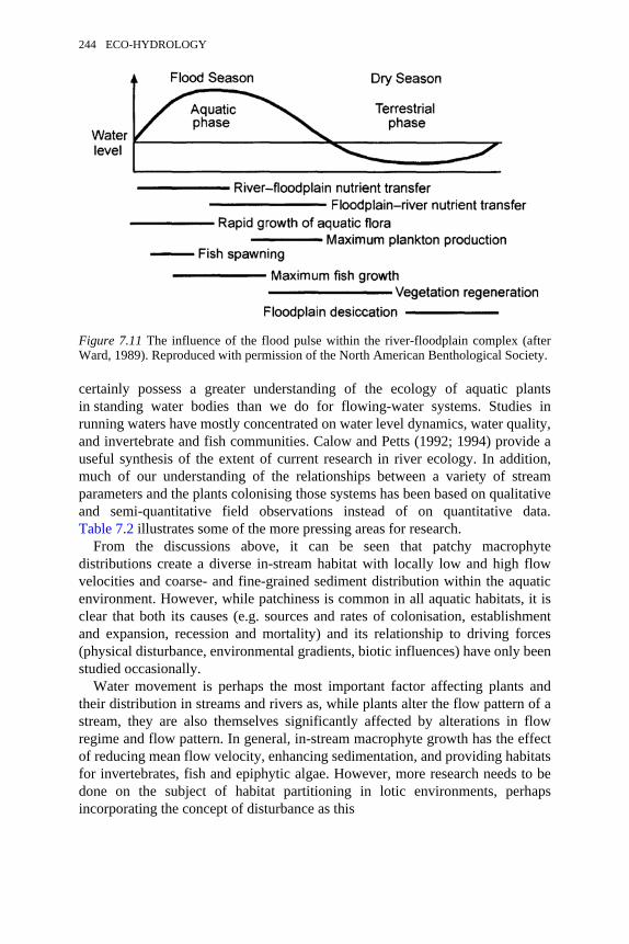
certainly possess a greater understanding of the ecology of aquatic plantsin standing water bodies than we do for flowing-water systems. Studies inrunning waters have mostly concentrated on water level dynamics, water quality,and invertebrate and fish communities. Calow and Petts (1992; 1994) provide auseful synthesis of the extent of current research in river ecology. In addition,much of our understanding of the relationships between a variety of streamparameters and the plants colonising those systems has been based on qualitativeand semi-quantitative field observations instead of on quantitative data.Table 7.2 illustrates some of the more pressing areas for research.
From the discussions above, it can be seen that patchy macrophytedistributions create a diverse in-stream habitat with locally low and high flowvelocities and coarse- and fine-grained sediment distribution within the aquaticenvironment. However, while patchiness is common in all aquatic habitats, it isclear that both its causes (e.g. sources and rates of colonisation, establishmentand expansion, recession and mortality) and its relationship to driving forces(physical disturbance, environmental gradients, biotic influences) have only beenstudied occasionally.
Water movement is perhaps the most important factor affecting plants andtheir distribution in streams and rivers as, while plants alter the flow pattern of astream, they are also themselves significantly affected by alterations in flowregime and flow pattern. In general, in-stream macrophyte growth has the effectof reducing mean flow velocity, enhancing sedimentation, and providing habitatsfor invertebrates, fish and epiphytic algae. However, more research needs to bedone on the subject of habitat partitioning in lotic environments, perhapsincorporating the concept of disturbance as this
Figure 7.11 The influence of the flood pulse within the river-floodplain complex (afterWard, 1989). Reproduced with permission of the North American Benthological Society.
244 ECO-HYDROLOGY
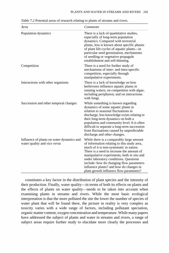
Table 7.2 Potential areas of research relating to plants of streams and rivers.
Area Comments
Population dynamics There is a lack of quantitative studies,especially of long-term populationdynamics. Compared with terrestrialplants, less is known about specific phasesof plant life-cycles of aquatic plants—inparticular seed germination, mechanismsof seedling or vegetative propaguleestablishment and self-thinning.
Competition There is a need for further study ofmechanisms of inter- and intra-specificcompetition, especially throughmanipulative experiments.
Interactions with other organisms There is a lack of knowledge on howherbivores influence aquatic plants inrunning waters; on competition with algae,including periphyton; and on interactionswith fungi.
Succession and other temporal changes While something is known regardingdynamics of some aquatic plants inrelation to seasonal fluctuations indischarge, less knowledge exists relating totheir long-term dynamics on both apopulation and community level. It is oftendifficult to separate a long-term successionfrom fluctuations caused by unpredictabledischarge and other changes.
Influence of plants on water dynamics andwater quality and vice versa
While there is a comparably large amountof information relating to this study area,much of it is non-systematic in nature.There is a need to increase the amount ofmanipulative experiments, both in situ andunder laboratory conditions. Questionsinclude: how do changing flow parametersinfluence plants? and how do changes inplant growth influence flow parameters?
constitutes a key factor in the distribution of plant species and the intensity oftheir production. Finally, water quality—in terms of both its effects on plants andthe effects of plants on water quality—needs to be taken into account whenexamining plants in streams and rivers. While the most basic ecologicalinterpretation is that the more polluted the site the lower the number of species ofwater plant that will be found there, the picture in reality is very complex astoxicity varies with a wide range of factors, including pollutant speciation,organic matter content, oxygen concentration and temperature. While many papershave addressed the subject of plants and water in streams and rivers, a range ofsubject areas require further study to elucidate more clearly the processes and
PLANTS AND WATER IN STREAMS AND RIVERS 245
interactions occurring between the flowing water environment and the plant lifefound therein (cf. Table 7.2). For example, in discussing the effects of currentvelocity on plant species richness along rivers, Nilsson (1987) has highlighted anumber of gaps in the knowledge base relating to aquatic vegetation that couldusefully be addressed, pointing out that information is needed on therelationships between edaphic conditions, vegetative dispersal, seed availabilityand germination success along the current velocity gradient, as well as on gapformation and deposition of propagules. More than a decade later, this wouldstill appear to be the case. Johansson and Nilsson (1993) conclude that modellingof vegetation dynamics should aim at combining within-site processes likecompetition, stress and disturbance with between-site processes (i.e. hydrochory)as mechanisms structuring plant communities. Sand-Jensen et al. (1989) havealso pointed out that, despite the marked influence that submerged macrophyteshave on lowland stream systems, little is known about their seasonal development,or the factors that result in variation in macrophyte development and abundanceboth among streams and between years in a particular stream. Future effortshould concentrate on these and related areas of study because, as the abovediscussion shows, while only a relatively small number of species can growsuccessfully in-stream, their occurrence in streams and rivers has importanthydrological and ecological consequences. In many cases too, theseconsequences have considerable economic implications.
REFERENCES
Angelier, E. (1953) Recherches écologiques et biogéographiques sur la faune de sablessubmergés, Archives de Zoologie Expérimental et Génerale 90:37–161.
Bakry, M.F., Gates, T.K. and Khattab, A.F. (1992) Field-measured hydraulic resistancecharacteristics in vegetation-infested canals, Journal of Irrigation and DrainageEngineering 118:256–274.
Barnes, H.H. (1967) Roughness characteristics of natural channels. US Geological SurveyWater Supply Paper 1949, US Government Printing Office, Washington DC.
Bathurst, J.C. (1981) Discussion of bar resistance of gravel bed streams, Journal of theHydraulics Division, ASCE 107:1276–1278.
Bathurst, J.C. (1985) Literature Review on Some Aspects of Gravel Bed Rivers,Wallingford: Institute of Hydrology.
Bathurst, J.C. (1997) Environmental river flow hydraulics, in Thorne, C.R., Hey, R.D. andNewson, M.D. (eds) Applied Fluvial Geomorphology for River Engineering andManagement, Chichester: Wiley, pp. 69–93.
Begon, M., Harper, J.L. and Townsend, C.R. (1990) Ecology: Individuals, Populationsand Communities, Oxford: Blackwell.
Bilby, R.E. and Likens, G.E. (1980) Importance of organic debris dams in the structureand function of stream ecosystems, Ecology 61:1107–1113.
Bijl, L. van der, Sand-Jensen, K. and Hjermind, A.L. (1989) Photosynthesis and canopystructure of a submerged plant, Potamogeton pectinatus, in a Danish lowland stream,Journal of Ecology 72:947–962.
246 ECO-HYDROLOGY
Bisson, P.A., Bilby, R.E., Bryant, M.D., Dolloff, C.A., Grette, G.B., House, R.A.,Murphy, M.L., Koski, K.V. and Sedell, J.R. (1987) Large woody debris in forestedstreams in the Pacific northwest: past, present and future, in Salo, E.O. and Cundy,T.W. (eds) Streamside Management: forestry and Fishery Interactions, Seattle:College of Forest Resources, University of Washington, pp. 143–190.
Blom, C.W.P.M., Bögemann, G.M., Laan, P., van der Sman, A.J.M., van de Steeg, H.M.and Voesenek, L.A.C.J. (1990) Adaptations to flooding in plants from river areas,Aquatic Botany 38:29–47.
Brändle, R., Cizková, H. and Pokorny, J. (1996) Adaptation Strategies in Wetland Plants:Links between Ecology and Physiology, Uppsala: Opulus Press.
Broadhurst, L.J., Heritage, G.L., van Niekerk, A.W. and James, C.S. (in press)Translating Discharge into Local Hydraulic Conditions on the Sabie River: AnAssessment of Channel Roughness, Pretoria: Water Research Commission Report No.474/2/96.
Brooker, M.P., Morris, D.L. and Wilson, C.J. (1978) Plant-flow relationships in the RiverWye catchment, in Proceedings of the European Weed Research Symposium, 5thSymposium on Aquatic Weeds, Amsterdam: European Weed Research Society,pp. 63–69.
Brookes, A. (1995) The importance of high flows for riverine environments, in Harper,D.M. and Ferguson, A.J.D. (eds) The Ecological Basis for River Management,Chichester: Wiley, pp. 33–49.
Brown S. and Lugo A.E. (1982) A comparison of structural and functional characteristicsof saltwater and freshwater forested wetlands, in Gopal B., Turner R.E., Wetzel R.G.and Whigham D.F. (eds) Wetlands Ecology and Management, Jaipur: InternationalScientific Publications.
Calow, P. and Petts, G.E. (eds) (1992) The Rivers Handbook, Volume 1. Oxford:Blackwell.
Calow, P. and Petts, G.E. (eds) (1994) The Rivers Handbook, Volume 2. Oxford:Blackwell.
Carpenter, S.R. and Lodge D.M. (1986) Effects of submersed macrophytes on eco-systemprocesses, Aquatic Botany 26:341–370.
Cook, C.D.K. (1996) Aquatic Plant Book, Amsterdam: SPB Academic.Dale, H.M. and Gillespie, T.J. (1977) The influence of submersed aquatic plants on
temperature gradients in shallow water bodies, Canadian Journal of Botany 55:2216–2225.
Dawson, F.H. (1976) The annual production of the aquatic macrophyte Ranunculuspenicillatus var. calcareous, Aquatic Botany 2:51–73.
Dawson, F.H. (1978) The seasonal effects of aquatic plant growth on the flow of water ina stream, in Proceedings of the European Weed Research Symposium, 5thSymposium on Aquatic Weeds, Amsterdam: European Weed Research Society,pp. 71–78.
Day, R.T, Keddy, P.A., McNeill, J. and Carleton, T. (1988) Fertility and disturbancegradients: a summary model for riverine marsh vegetation, Ecology 69: 1044–1054.
Dhillon, M.S., Mukka, M.S. and Hwang, Y.-S. (1982) Allelochemicals produced by thehydrophyte Myriophyllum spicatum affecting mosquitoes and midges, Journal ofChemical Ecology 8:517–526.
Dingman, S.L. (1984) Fluvial Hydrology, New York: Freeman, 383 pp.
PLANTS AND WATER IN STREAMS AND RIVERS 247

Dodds, W.K. (1991) Micro-environmental characteristics of filamentous algalcommunities in flowing freshwaters , Freshwater Biology 25:199–209.
Dole-Olivier, M.J. and Marmonier, P. (1992) Patch dynamics of interstitial communities:prevailing factors, Freshwater Biology 27:177–191.
Farmer, A.M. and Spence, D.H.N. (1987) Flowering, germination and zonation of thesubmerged aquatic plant Lobelia dortmanna L., Journal of Ecology 75: 1065–1076.
Fennessy, S. (1993) Riparian Buffer Srips: Their Effectiveness for the Control ofAgricultural Pollution, London: Institute for European Environmental Policy Report210/89, University College.
Forman, R.T.T. and Godron, M. (1986) Landscape Ecology, New York: Wiley.French, T.D. and Chambers, P.A. (1996) Habitat partitioning in riverine macrophyte
communities, Freshwater Biology 36:509–520.Gilvear, D.J. and Bravard, J.-P. (1996) Geomorphology of temperate rivers, in Petts, G.E.
and Amoros, C. (eds) Fluvial Hydrosystems, London: Chapman & Hall, pp. 68–97.Gopal, B. and Goel, U. (1993) Competition and allelopathy in aquatic plant communities,
Botanical Review 59:155–210.Grace, J.B. (1987) The impact of pre-emption on the zonation of two Typha species along
lakeshores, Ecological Monographs 57:283–303.Gregory, K.J. (1992) Vegetation and river channel process interactions, in Boon, P.J.,
Calow, P. and Petts, G.E. (eds) River Conservation and Management, Chichester:Wiley, pp. 255–269.
Grime, J.P. (1979) Plant Strategies and Vegetation Processes, Chichester: Wiley.Gurnell, A.M. (1997) Woody debris and river—floodplain interactions, in Large, A.R.G.
(ed.), Floodplain Rivers: Hydrological Processes and Ecological Significance,Newcastle: British Hydrological Society Occasional Paper No. 8, University ofNewcastle upon Tyne, pp. 6–17.
Gurnell, A.M. and Gregory, K.J. (1987) Vegetation characteristics and the prediction ofrunoff: analysis of an experiment in the New Forest, Hampshire, HydrologicalProcesses 1:125–142.
Gurnell, A.M., Gregory, K.J. and Petts, G.E. (1995) The role of coarse woody debris inforest aquatic habitats: implications for management, Aquatic Conservation: Marineand Freshwater Ecosystems 5:143–166.
Ham, S.F., Cooling, D.A., Hiley, P.D., McLeish, P.R., Scorgie, H.R.A. and Berrie, A.D.(1982) Growth and recession of aquatic macrophytes on a shaded section of theRiver Lambourn, England, from 1971 to 1980, Freshwater Biology 12:1–15.
Haslam, S.M. (1978) River Plants: The Aquatic Vegetation of Watercourses, Cambridge:Cambridge University Press.
Haslam, S.M. (1987) River Plants of Western Europe: The Macrophytic Vegetation ofWatercourses of the European Economic Community, Cambridge: CambridgeUniversity Press.
Haslam, S.M. (1990) River Pollution: An Ecological Perspective, Chichester: Wiley.Haycock, N.E. and Pinay, G. (1993) Groundwater-nitrate dynamics in grass and poplar
vegetated riparian buffer strips during the winter, Journal of Environmental Quality22:273–278.
Hey, R.D. (1988) Bar form resistance in gravel bed rivers, Journal of the HydraulicsDivision, ASCE 114:1498–1508.
Hicken, E.J. (1984) Vegetation and river channel dynamics, Canadian Geographer 28:111–126.
248 ECO-HYDROLOGY
Hill, W.R., Ryon, M.G. and Schilling, E.M. (1995) Light limitation in a stream ecosystem:responses by primary producers and consumers, Ecology 76: 1297–1309.
Holland, M.M. (1988) SCOPE/MAB technical consultations on landscape boundaries:report of a SCOPE/MAB workshop on ecotones, Biology International Special Issue17:47–106.
Holmes, N.T.H. (1983) Typing British Rivers According to their Flora, Focus on NatureConservation 4, Peterborough: Nature Conservancy Council.
Hutchinson, G.E. (1975) A Treatise on Limnology. III Limnological Botany, New York:Wiley.
Hydraulics Research (1992) The Hydraulic Roughness of Vegetated Channels, HRWallingford Report SR 305, Wallingford: Hydraulics Research.
Hynes, H.B.N. (1970) The Ecology of Running Waters, Liverpool: Liverpool UniversityPress.
Jackson, M.B., Davies, D.D. and Lambers, H. (eds) (1991) Plant Life Under OxygenDeprivation: Ecology, Physiology and Biochemistry, Amsterdam: SPB Academic.
Jeffries, M. and Mills, D. (1994) Freshwater Ecology: Principles and Applications,Chichester: Wiley.
Johansson, M.E. and Nilsson, C. (1993) Hydrochory, population dynamics anddistribution of the clonal aquatic plant Ranunculus lingua, Journal of Ecology 81:81–91.
Junk, W.G., Bayley, P.B. and Sparks, R.E. (1989) The flood pulse concept in river-flooding systems, Canadian Journal of Fisheries and Aquatic Sciences 106:110–127.
Kouwen, N. and Li, R.M. (1980) Biomechanics of vegetative channel linings, Journal ofthe Hydraulics Division, ASCE 106:1085–1103.
Large, A.R.G. and Petts, G.E. (1992) Buffer Zones for Riverbank Conservation, NationalRivers Authority Project 340/Y/5, Loughborough: International Centre of LandscapeEcology, Loughborough University, 71 pp.
Large, A.R.G. and Petts, G.E. (1994) Rehabilitation of river margins, in Calow, P. andPetts, G.E. (eds) The Rivers Handbook, Volume 2, Oxford: Blackwell Scientific,pp. 401–418.
Large, A.R.G., Pautou, G. and Amoros, C. (1996) Primary production and primaryproducers, in Petts, G.E. and Amoros, C. (eds) Fluvial Hydrosystems, London:Chapman & Hall, pp. 117–136.
Losee, R.F. and Wetzel, R.G. (1993) Littoral flow rates within and around submersedmacrophyte communities, Freshwater Biology 29:7–17.
Lowrance, R., Leonard, R. and Sheridan, J. (1985) Managing riparian ecosystems tocontrol non-point pollution, Journal of Soil and Water Conservation 40:87–91.
Lucas, W.J. and Berry, J.A. (1985) Inorganic carbon transport in aquatic photosyntheticorganisms, Physiologia Plantarum 65:117–124.
Madsen, T.V. and Maberly, S.C. (1991) Diurnal variation in light and carbon limitation ofphotosynthesis by two species of submerged freshwater macrophyte with adifferential ability to use bicarbonate, Freshwater Biology 26:175–187.
Malanson, G.P. (1993) Riparian Landscapes, Cambridge: Cambridge University Press.Marshall, E.J.P. and Westlake, D.F. (1978) Recent studies on the roles of aquatic
macrophytes in their ecosystem, in Proceedings of the European Weed ResearchSymposium, 5th Symposium on Aquatic Weeds, Amsterdam: European WeedResearch Society, pp. 183–188.
PLANTS AND WATER IN STREAMS AND RIVERS 249
Masterman, R. and Thorne, C.R. (1992) Predicting influence of bank vegetation onchannel capacity, Journal of Hydraulic Engineering 118:1052–1058.
Miller, B.A. and Wenzel, H.G. (1985) Analysis and simulation of low flow hydraulics.Journal of Hydraulic Engineering 111:1429–1446.
Moeslund, B. Løjtnant, B., Mathiesen, H., Mathiesen, L., Pedersen, A., Thyssen, N. andSchou, J.C. (1990) Danske Vandplanter, Danish Environmental Protection Agency.
Muscutt, A.D., Harris, G.L., Bailey, S.W. and Davies, D.B. (1993) Buffer zones toimprove water quality: a review of their potential use in UK agriculture, Agriculture,Ecosystems and Environment 45:59–77.
Naiman, R.J., Décamps, H., Pastor, J. and Johnston, C.A. (1988) The potential importanceof boundaries to fluvial ecosystems, Journal of the North American BenthologicalSociety 7:289–306.
Naiman, R.J. and Décamps, H. (eds) (1990) The Ecology and Management of Aquatic-Terrestrial Ecotones, Carnforth: UNESCO Paris and Parthenon Publishing Group.
Newall, A.M. (1995) The micro-flow environment of aquatic plants: an ecologicalperspective, in Harper, D.M, and Ferguson, A.J.D. (eds) The Ecological Basis forRiver Management, Chichester: Wiley, pp. 79–92.
Newson, M.D. (1992) Land, Water and Development: River Basin Systems and theirSustainable Management, London: Routledge.
Nilsson, C. (1987) Distribution of stream-edge vegetation along a gradient of currentvelocity, Journal of Ecology 75:513–522.
Nilsson, C. and Grelsson, G. (1989) The effects of litter displacement on riverbankvegetation, Canadian Journal of Botany 68:735–741.
Nilsson, C., Gardfjel, M. and Grelsson, G. (1991) Importance of hydrochory in structuringplant communities along rivers, Canadian Journal of Botany 69: 2631–2633.
Nilsson, C., Grelsson, G., Johansson, M. and Sperens, U. (1989) Patterns of plant speciesrichness along riverbanks, Ecology 70:77–84.
Orghidan, T. (1955) Un nou domeniu de viata acvatica subterana: ‘biotopul hiporeic’,Buletin Stiintific sectia de Biologie si stiinte Agricole si sectia de Geologie si GeografieVII: 657–676.
Osborne, L.L. and Kovacic, D.A. (1993) Riparian vegetated buffer strips in water-qualityrestoration and management, Freshwater Biology 29:243–258.
Petts, G.E. (1994) Rivers: dynamic components of catchment ecosystems, in Calow, P.and Petts, G.E. (eds) The Rivers Handbook, Volume 2, Oxford: Blackwell, pp. 3–22.
Petts, G.E. and Foster, I.D.L. (1985) Rivers and Landscape, London: Edward Arnold.Philips, G.L., Eminson, D.F. and Moss, B. (1978) A mechanism to account formacrophyte decline in progressively eutrophicated freshwaters , Aquatic Botany 4:103–126.
Pickett, S.T.A. and White, P.S. (1985) Patch dynamics: a synthesis, in Pickett, S.T.A. andWhite, P.S. (eds) The Ecology of Natural Disturbances and Patch Dynamics, NewYork: Academic Press, pp. 371–384.
Pinay, G., Décamps, H., Chauvet, E. and Fustec, E. (1990) Functions of ecotones influvial systems, in Naiman, R.J. and Décamps, H. (eds) The Ecology andManagement of Aquatic-Terrestrial Ecotones, Carnforth: UNESCO Paris andParthenon Publishing Group, pp. 141–169.
Polunin, N. (1982) Processes contributing to the decay of reed (Phragmites australis)litter in fresh water, Archiv für Hydrobiologie 114:401–414.
250 ECO-HYDROLOGY
Polunin, N. (1984) The decomposition of emergent macrophytes in fresh water, Advancesin Ecological Research 14:115–166.
Prach, K., Large, A.R.G., and Jeník, J. (1996) River floodplains as ecological systems, inPrach, K., Jeník, J., and Large A.R.G. (eds) Floodplain Ecology and Management:The Luznice River in the Trebon Biosphere Reserve, Central Europe , Amsterdam:SPB Academic, pp. 1–9.
Pyšek, P. (1994) Ecological aspects of invasion by Heracleum mantegazzianum in theCzech Republic, in de Waal, L.C., Child, L.E., Wade, P.M. and Brock, J.H. (eds)Ecology and Management of Invasive Riverside Plants, Chichester: Wiley,pp. 45–54.
Pyšek, P. and Prach, K. (1993) Plant invasions and the role of riparian habitats—acomparison of four species alien to Central Europe, Journal of Biogeography 20:413–420.
Pyšek, P. and Prach, K. (1995) Invasion dynamics of Impatiens glandulifera—a centuryof spreading reconstructed, Biological Conservation 74:41–48.
Rattrey, M.R., Brown, J.M.A. and Howard-Williams, C. (1991) Sediment and water assources of nitrogen and phosphorus for submerged rooted aquatic macrophytes,Aquatic Botany 40:225–237.
Resh, V.H., Brown, A.V., Covich, A.P., Gurtz, M.E., Li, H.W., Minshall, G.W., Reice,S.R., Sheldon, A.L., Wallace, J.B. and Wissmar, R.C. (1988) The role of disturbancein stream ecology, Journal of the North American Benthological Society 7: 433–455.
Richards, K. (1982) Rivers: Form and Process in Alluvial Channels, London: Methuen.Rydlo, J. (1996) Water macrophytes in the section of the River Elbe in 1976, 1986 and
1996, Museum a soucasnost (Rydlia) 11:87–128.Sand-Jensen, K. (1987) Experimental control of bicarbonate use among freshwater and
marine macrophytes, in Crawford, R.M.M. (ed.) Plant Life in Aquatic andAmphibious Habitats, British Ecological Society Special Publication 5, Oxford:Blackwell, pp. 99–112.
Sand-Jensen, K. and Madsen, T.V. (1992) Patch dynamics of the stream macrophyteCallitriche cophocarpa, Freshwater Biology 27:277–282.
Sand-Jensen, K. and Mebus, J.R. (1996) Fine-scale patterns of water velocity withinmacrophyte patches in streams, Oikos 76:169–180.
Sand-Jensen, K., Jeppesen, E., Nielsen, K., van der Bijl, L., Hjermind, L., Nielsen, L.W.and Iversen, T.M. (1989) Growth of macrophytes and ecosystem consequences in alowland Danish stream, Freshwater Biology 22:15–32.
Sand-Jensen, K. Pedersen, M.F. and Nielsen, S.L. (1992) Photosynthetic use of inorganiccarbon among primary and secondary water plants in streams, Freshwater Biology27:283–293.
Schneider, R.L. and Sharitz, R.R. (1988) Hydrochory and regeneration in a bald-cypress-water Tupelo swamp forest, Ecology 69:1055–1063.
Sculthorpe, C.D. (1967) The Biology of Aquatic Vascular Plants, London: EdwardArnold.
Smith, R.J., Hancock, N.H. and Ruffini, J.L. (1990) Flood flow through tall vegetation,Agricultural Water Management 18:317–332.
Stephan, U. and Wychera, U. (1996) Analysis of flow velocity fluctuations in differentmacrophyte banks in a natural open channel, Proceedings of SymposiumEcohydraulics 2000, Quebec, Canada, June 1996, A191-A202.
PLANTS AND WATER IN STREAMS AND RIVERS 251
Teal, J.M. (1980) Primary production of benthic and fringing plant communities, inBarnes, R.S.K. and Mann, K.H. (eds) Fundamentals of Aquatic Ecosystems, Oxford:Blackwell, pp. 67–83.
Triska, F.J. and Cromack, K. (1980) The role of wood debris in forests and streams, inWaring, R.H. (ed.) Forests: Fresh Perspectives from Ecosystem Analysis, OregonState University, pp. 171–189.
Vannote, R.L., Minshall, G.W., Cummins, K.W., Sedell, J.R. and Cushing, C.E. (1980)The river continuum concept, Canadian Journal of Fisheries and Aquatic Sciences37:130–137.
Vought, L.B.-M., Dahl, J., Pedersen, C.L. and Lacoursière, J.O. (1994) Nutrient retentionin riparian ecotones, Ambio 23:342–348.
Ward, J.V. (1989) The four dimensional nature of lotic ecosystems, Journal of the NorthAmerican Benthological Society 8:2–8.
Ward, J.V. and Stanford, J.A. (1995) The serial discontinuity concept: extending themodel to floodplain rivers, Regulated Rivers: Research and Management 10:159–168.
Watson, D. (1987) Hydraulic effects of aquatic weeds in UK rivers, Regulated Rivers:Research and Management 1:211–227.
Watts, J.F. and Watts, G.D. (1990) Seasonal change in aquatic vegetation and its effect onchannel flow, in Thornes, J.B. (ed.) Vegetation and Erosion, Chichester: Wiley.
Welcomme, R.L. (1979) Fisheries Ecology ofFloodplain Rivers, London: Longman.Westlake, D.F. (1975) Macrophytes, in Whitton, B.A. (ed.) River Ecology, Oxford:
Blackwell, pp. 106–128.Westlake, D.F., Adams, M.S., Bindloss, M.E., Ganf, G.G., Gerloff, G.C., Hammer, U.T.,
Javornický, P., Koonce, J.F., Marker, A.F.H., McCracker, M.D., Moss, B.,Nauwerck, A., Pyrina, I.L., Steel, J.A.P., Tilzer, M. and Walters, C.J. (1980) Primaryproduction, in Le Cren, E.D. and Lowe-McConnell, R.H. (eds) The Functioning ofFreshwater Ecosystems, International Biological Programme 22, Cambridge:Cambridge University Press, pp. 141–246.
Wheeler, W.H. (1980) Effects of boundary layer transport on the fixation of carbon by thegiant kelp Macrocystis pyrifera, Marine Biology 56:103–110.
Wiegleb, G. (1988) Analysis of flora and vegetation in rivers: concepts and applications,in Symoens, J.J. (ed.) Vegetation of Inland Waters, Dordrecht: Kluwer, pp. 311–340.
Wilson, E.M. (1974) Engineering Hydrology, London: Macmillan Press. Wilson, S.D. andKeddy, P.A. (1986) Measuring diffuse competition along an environmental gradient:results from a shoreline plant community, American Naturalist 127:862–869.
Wilson, S.D. and Keddy, P.A. (1991) Competition, survivorship and growth inmacrophyte communities, Freshwater Biology 25:331–337.
Wright, J.F, Cameron, A.C., Hiley, P.D. and Berrie, A.D. (1982) Seasonal changes inbiomass of macrophytes on shaded and unshaded sections of the River Lambourn,England, Freshwater Biology 12:271–283.
252 ECO-HYDROLOGY
8PLANTS AND WATER IN AND
ADJACENT TO LAKESRobert G.Wetzel
INTRODUCTION
The structure, metabolism and biogeochemistry of a lake are strongly coupled toinputs from its drainage basin. A lake reflects the developmental conditions anddisturbances within the catchment, its drainage streams, and the vegetationabove, at and below the land-water interface.
Those allochthonous inputs are largely transported to the lake in particulateand especially soluble compounds with water. Inputs from atmospheric sourcesare usually small in comparison with loadings from ground and surface-watersources. These compounds, particularly nutrients, influence the autochthonousdevelopment and productivity of micro- and macro-vegetation within the lake.The vegetation in turn can have profound effects on the movements of waterwithin the basin, export of water from the basin via evapotranspiration, andalteration of habitats within lakes. Indeed, the macrovegetation influences theentire ontogeny (successional development) of lake ecosystems (Wetzel, 1979;1983; 1990; 1992).
THE LAND-WATER INTERFACE REGION OF AQUATICECOSYSTEMS
The land-water interface zone includes a large area of most lake ecosystems thatextends from hydrosoils that are at least periodically saturated at the uplandboundary through to and including the wetland and littoral areas to depths thathave sufficient light to support larger aquatic plants (Wetzel, 1983). Thisinterface zone constitutes an intensely metabolically active region that stronglyinfluences the biotic metabolism of both standing and flowing fresh waters.Much of the nutrient loading, cycling and recycling within many fresh waters iscontrolled by the metabolism of the wetland and littoral macrophytes and theirassociated microflora (Wetzel, 1990). Because most aquatic ecosystems occur interrain of gentle slopes with very small elevational gradients and are small inarea and shallow in depth (Figure 8.1), the wetland-littoral components usually
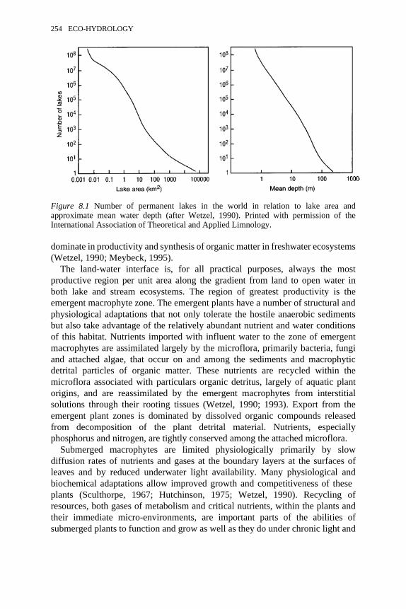
dominate in productivity and synthesis of organic matter in freshwater ecosystems(Wetzel, 1990; Meybeck, 1995).
The land-water interface is, for all practical purposes, always the mostproductive region per unit area along the gradient from land to open water inboth lake and stream ecosystems. The region of greatest productivity is theemergent macrophyte zone. The emergent plants have a number of structural andphysiological adaptations that not only tolerate the hostile anaerobic sedimentsbut also take advantage of the relatively abundant nutrient and water conditionsof this habitat. Nutrients imported with influent water to the zone of emergentmacrophytes are assimilated largely by the microflora, primarily bacteria, fungiand attached algae, that occur on and among the sediments and macrophyticdetrital particles of organic matter. These nutrients are recycled within themicroflora associated with particulars organic detritus, largely of aquatic plantorigins, and are reassimilated by the emergent macrophytes from interstitialsolutions through their rooting tissues (Wetzel, 1990; 1993). Export from theemergent plant zones is dominated by dissolved organic compounds releasedfrom decomposition of the plant detrital material. Nutrients, especiallyphosphorus and nitrogen, are tightly conserved among the attached microflora.
Submerged macrophytes are limited physiologically primarily by slowdiffusion rates of nutrients and gases at the boundary layers at the surfaces ofleaves and by reduced underwater light availability. Many physiological andbiochemical adaptations allow improved growth and competitiveness of these plants (Sculthorpe, 1967; Hutchinson, 1975; Wetzel, 1990). Recycling ofresources, both gases of metabolism and critical nutrients, within the plants andtheir immediate micro-environments, are important parts of the abilities ofsubmerged plants to function and grow as well as they do under chronic light and
Figure 8.1 Number of permanent lakes in the world in relation to lake area andapproximate mean water depth (after Wetzel, 1990). Printed with permission of theInternational Association of Theoretical and Applied Limnology.
254 ECO-HYDROLOGY
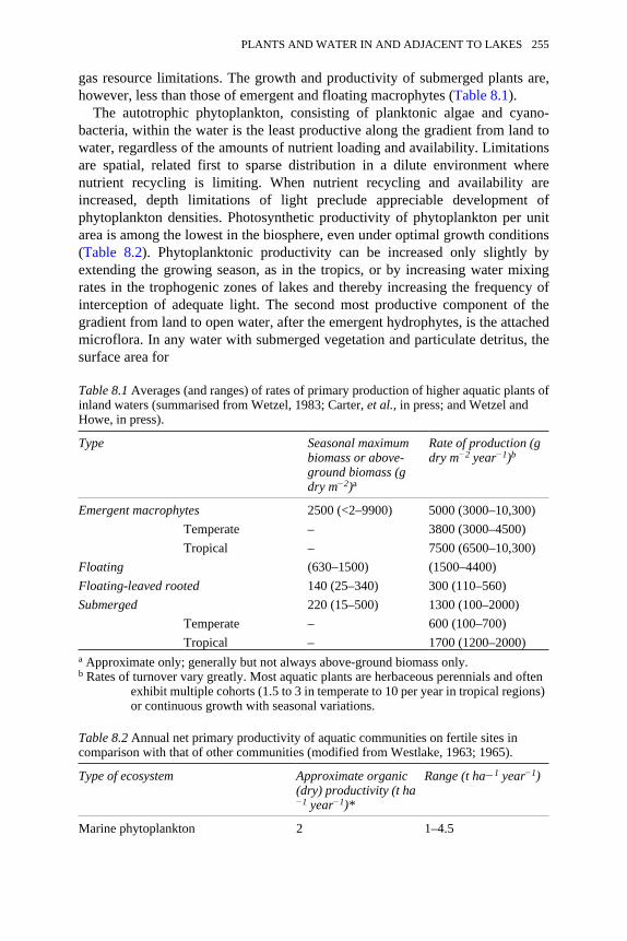
gas resource limitations. The growth and productivity of submerged plants are,however, less than those of emergent and floating macrophytes (Table 8.1).
The autotrophic phytoplankton, consisting of planktonic algae and cyano-bacteria, within the water is the least productive along the gradient from land towater, regardless of the amounts of nutrient loading and availability. Limitationsare spatial, related first to sparse distribution in a dilute environment wherenutrient recycling is limiting. When nutrient recycling and availability areincreased, depth limitations of light preclude appreciable development ofphytoplankton densities. Photosynthetic productivity of phytoplankton per unitarea is among the lowest in the biosphere, even under optimal growth conditions(Table 8.2). Phytoplanktonic productivity can be increased only slightly byextending the growing season, as in the tropics, or by increasing water mixingrates in the trophogenic zones of lakes and thereby increasing the frequency ofinterception of adequate light. The second most productive component of thegradient from land to open water, after the emergent hydrophytes, is the attachedmicroflora. In any water with submerged vegetation and particulate detritus, thesurface area for
Table 8.1 Averages (and ranges) of rates of primary production of higher aquatic plants ofinland waters (summarised from Wetzel, 1983; Carter, et al., in press; and Wetzel andHowe, in press).
Type Seasonal maximumbiomass or above-ground biomass (gdry m−2)a
Rate of production (gdry m−2 year−1)b
Emergent macrophytes 2500 (<2–9900) 5000 (3000–10,300)Temperate – 3800 (3000–4500)Tropical – 7500 (6500–10,300)
Floating (630–1500) (1500–4400)Floating-leaved rooted 140 (25–340) 300 (110–560)Submerged 220 (15–500) 1300 (100–2000)
Temperate – 600 (100–700)Tropical – 1700 (1200–2000)
a Approximate only; generally but not always above-ground biomass only.b Rates of turnover vary greatly. Most aquatic plants are herbaceous perennials and often
exhibit multiple cohorts (1.5 to 3 in temperate to 10 per year in tropical regions)or continuous growth with seasonal variations.
Table 8.2 Annual net primary productivity of aquatic communities on fertile sites incomparison with that of other communities (modified from Westlake, 1963; 1965).
Type of ecosystem Approximate organic(dry) productivity (t ha−1 year−1)*
Range (t ha−1 year−1)
Marine phytoplankton 2 1–4.5
PLANTS AND WATER IN AND ADJACENT TO LAKES 255
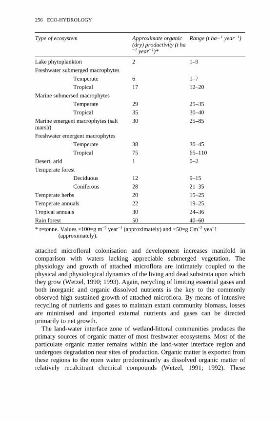
Type of ecosystem Approximate organic(dry) productivity (t ha−1 year−1)*
Range (t ha−1 year−1)
Lake phytoplankton 2 1–9Freshwater submerged macrophytes
Temperate 6 1–7Tropical 17 12–20
Marine submersed macrophytesTemperate 29 25–35Tropical 35 30–40
Marine emergent macrophytes (saltmarsh)
30 25–85
Freshwater emergent macrophytesTemperate 38 30–45Tropical 75 65–110
Desert, arid 1 0–2Temperate forest
Deciduous 12 9–15Coniferous 28 21–35
Temperate herbs 20 15–25Temperate annuals 22 19–25Tropical annuals 30 24–36Rain forest 50 40–60* t=tonne. Values ×100=g m−2 year−1 (approximately) and ×50=g Cm−2 yea−1
(approximately).
attached microfloral colonisation and development increases manifold incomparison with waters lacking appreciable submerged vegetation. Thephysiology and growth of attached microflora are intimately coupled to thephysical and physiological dynamics of the living and dead substrata upon whichthey grow (Wetzel, 1990; 1993). Again, recycling of limiting essential gases andboth inorganic and organic dissolved nutrients is the key to the commonlyobserved high sustained growth of attached microflora. By means of intensiverecycling of nutrients and gases to maintain extant community biomass, lossesare minimised and imported external nutrients and gases can be directedprimarily to net growth.
The land-water interface zone of wetland-littoral communities produces theprimary sources of organic matter of most freshwater ecosystems. Most of theparticulate organic matter remains within the land-water interface region andundergoes degradation near sites of production. Organic matter is exported fromthese regions to the open water predominantly as dissolved organic matter ofrelatively recalcitrant chemical compounds (Wetzel, 1991; 1992). These
256 ECO-HYDROLOGY

dissolved organic compounds of wetland-littoral origins function in severalimportant ways in aquatic ecosystems. The dissolved organic compounds, oftendominated by organic acids and polyphenolic substances of higher plant origin,have an array of regulatory functions on the availability of metals, inorganic andorganic micronutrients, carbonate and clay particle reactivities, and extracellularenzyme activities, among others (Wetzel, 1992). The dissolved organic matterforms a large reservoir of organic matter, usually an order of magnitude or moregreater than particulate organic matter. Although decomposed slowly (c. 1percent per day), the collective microbial metabolism is a major component ofthe energy dissipation of the ecosystem (Wetzel, 1995).
MOVEMENTS OF WATER TO AND WITHIN LAKES
The water balance of a lake is evaluated from the change in the water volume ofthe lake per unit time. In some cases, changes in lake volume can be calculatedfrom changes in lake area. The change in storage is equal to the rate of inflowfrom all sources minus the rate of water loss.
Water income to a lake or reservoir includes several sources:
1 Precipitation (P) directly on the lake surface. Most lakes exist in exorheicregions, within which rivers originate and from which they flow to the sea,and receive a relatively small proportion (<10 percent) of their total waterincome from direct precipitation. This percentage varies greatly, however,and increases in very large lakes. Extreme examples include Lake Victoriaof equatorial East Africa, which receives most (>70 percent) of its waterfrom precipitation on its surface (Kilham and Kilham, 1990).
2 Water from surface influents (R) of the drainage basin. Many lakes ofendorheic regions, within which rivers arise but never reach the sea, receivenearly all of their water from runoff. The rate of runoff from the drainagebasin and corresponding changes in lake level are influenced by the natureof the soil and vegetation cover of the drainage basin (cf. Wetzel, 1983;Likens, 1985).
3 Groundwater seepage (G.) below the surface of the lake. Seepage ofgroundwater is commonly a major source of water for lakes in rock basinsand lake basins in glacial tills that extend well below the water table. Sub-lacustrine groundwater seepage represents a major source of water flowinto, and out of, karst and doline lakes of limestone substrata. In wetlandsand littoral areas of lakes, there is often a complex seepage hydrology withgroundwater flow oscillating between upwelling and downwelling. Thiscomplex behaviour is mediated by variations in precipitation andevapotranspiration.
4 Groundwater entering lakes as discrete springs. Sub-lacustrine springs fromgroundwater occur frequently in hard water lakes of calcareous drift regions,where the basin is effectively sealed from groundwater seepage by deposits
PLANTS AND WATER IN AND ADJACENT TO LAKES 257
within the basin (e.g. Wetzel, 1965; 1966; Wetzel and Otsuki, 1974). Suchgroundwater inputs are often closely coupled to rates of precipitation andevapotranspiration. These inputs vary with any modifications, such asclimate changes, to rates of precipitation and evaporation. For example, inthe Dead Sea contributions from springs and shore seepage decreased asriver influents were purloined by partial diversions (Serruya and Pollinger,1984).
Losses of water occur by flow from an outlet (D) in drainage lakes and byseepage into the groundwater through the basin walls in seepage lakes.Deposition of clays, silts and carbonates commonly forms a very effective seal indrainage lakes, from which most or all of the outflow leaves by a surface outlet.In seepage lakes, the sediments over much of the deeper portions of the basinalso usually form an effective seal; losses to groundwater (Go) usually occur fromthe uppermost portions (<2 m depth) of the basin in these lakes.
Further losses of water occur directly by evaporation (E), or byevapotranspiration from emergent and floating-leaved aquatic macrophytes. Theextent and rates of evaporative losses are highly variable according to season andlatitude, and are greatest in endorheic regions. Closed lakes of semi-arid regionscommonly have no outflow and lose water only by evaporation. Because of themajor importance of aquatic macrophytes on the water budgets of lakes, thisecological mediation of water fluxes will be treated separately (see ‘Plants ascontrols on lake hydrological processes’, below).
The water balance states that the rate of change of the lake volume (V) withtime (t) is the difference between the water input and output rates (L3T−1)(Hutchinson, 1957; Szesztay, 1974; Mason et al., 1994), expressed as adifferential equation:
(8.1)
Each of these hydrological components is dynamic and optimally requirescontinuous measurement over large spatial areas in order to evaluate accuratelythe water budget of a lake. Uncertainty boundaries and variations betweenmeasurements within spatial distributions must be evaluated (Winter, 1981).Some atmospheric components of a water budget such as precipitation are variablespatially at relatively small distances (several kilometres) even though controlledby circulation of the atmosphere. Continuous measurement of other parameters isless reliable. For example, evaporative loss of water vapour from a water body iscontrolled by wind and vapour fluxes over the water body (Winter, 1995), both ofwhich are very variable.
The most accurate method of determining evaporation over periods of monthsor more is by the energy budget method, which is expensive in terms ofinstruments and labour. Gains and losses of heat from all sources of radiationfluxes, latent heat, sensible heat, precipitation, surface water and groundwater
258 ECO-HYDROLOGY
must be evaluated (Figure 8.2). The complexities of the energy budget method ofevaluating evaporation in lakes is treated in detail by Brutsaert (1982), Hostetler(1995), Imboden and Wuest (1995), and Winter (1995). Surface water fluxes canbe measured accurately both directly by river inflows/outflows and indirectly byvariations in lake depth and area.
Subsurface inputs and losses of water can be measured directly, although thisis often difficult and demanding to accomplish accurately, with in situ underwaterpiezometers (cf. Lee, 1977; 1985; Lee and Cherry, 1978; Lee and Harvey, 1996).Seepage measurements give some insights into subsurface loadings and allowlimited application of two- and three-dimensional models of groundwater flowdynamics. Advected groundwater and its energy contribute to the mass andenergy budgets of closed lakes. For example, advected groundwater accounts formore than 50 percent of the annual water input to a moderately sized (40 ha)closed lake in northern Minnesota, USA (Sturrock et al., 1992). More than 50percent of the water loss from the lake occurs annually by groundwater flow.*Even though seepage into the lake is large, groundwater contributes little thermalenergy input to the lake, because the groundwater flowing into the lake isrelatively cold at c. 7 °C. Similarly, because the lake water is warm for only briefperiods in the summer, seepage from the basin results in only small losses ofthermal energy to groundwater.
Although groundwater energy inputs and losses may not affect evaporation inmajor ways, these subsurface inputs can be of major importance in the loading ofinorganic and organic solutes that influence biotic distributions within lakes andtheir growth and productivity. Temporal and spatial patterns of seepage varygreatly in lake sediments because of heterogeneous sediment composition (e.g.Lee, 1977; Shaw and Prepas, 1990), transpiration from littoral and nearshorewetland vegetation (see ‘plants as controls on lake hydrological processes’,below), and non-uniform bending of groundwater flow paths where a slopingwater table from surrounding terrestrial deposits meets the flat lake surface(Winter, 1995). Because energy storage and losses are related to mass rather thanvolume, additional measures of density are required for snow and ice. Means ofmeasurement and estimation are summarised in Wetzel and Likens (1991). Oncethe densities of the snow and ice types have been determined, then latent heateffects on storage and water fluxes, especially for evaporation, condensation andsublimation, can be estimated. Energy budgets must be corrected for latent heatof fusion of ice, particularly when ice cover is considerable (e.g. Adams andLasenby, 1978; Wetzel, 1983).
Changes in lake volume determined by continuous stage height measurementsof the lake surface and detailed bathymetry integrate all fluxes to and from the
* Whether groundwater flows to or from a lake often depends on transpiration fromlittoral vegetation and its effect on lakeshore water tables (see ‘plants as controls on lakehydrological processes’, below).
PLANTS AND WATER IN AND ADJACENT TO LAKES 259
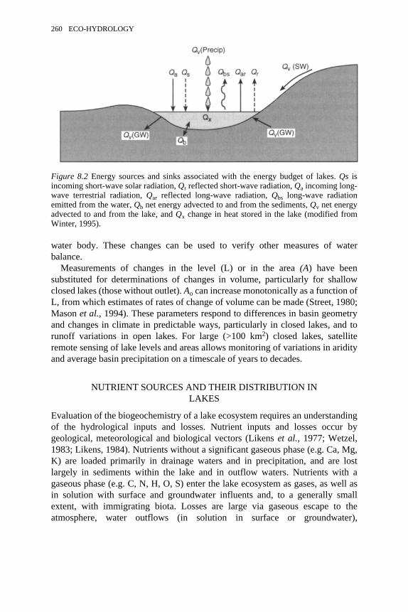
water body. These changes can be used to verify other measures of waterbalance.
Measurements of changes in the level (L) or in the area (A) have beensubstituted for determinations of changes in volume, particularly for shallowclosed lakes (those without outlet). Ao can increase monotonically as a function ofL, from which estimates of rates of change of volume can be made (Street, 1980;Mason et al., 1994). These parameters respond to differences in basin geometryand changes in climate in predictable ways, particularly in closed lakes, and torunoff variations in open lakes. For large (>100 km2) closed lakes, satelliteremote sensing of lake levels and areas allows monitoring of variations in aridityand average basin precipitation on a timescale of years to decades.
NUTRIENT SOURCES AND THEIR DISTRIBUTION INLAKES
Evaluation of the biogeochemistry of a lake ecosystem requires an understandingof the hydrological inputs and losses. Nutrient inputs and losses occur bygeological, meteorological and biological vectors (Likens et al., 1977; Wetzel,1983; Likens, 1984). Nutrients without a significant gaseous phase (e.g. Ca, Mg,K) are loaded primarily in drainage waters and in precipitation, and are lostlargely in sediments within the lake and in outflow waters. Nutrients with agaseous phase (e.g. C, N, H, O, S) enter the lake ecosystem as gases, as well asin solution with surface and groundwater influents and, to a generally smallextent, with immigrating biota. Losses are large via gaseous escape to theatmosphere, water outflows (in solution in surface or groundwater),
Figure 8.2 Energy sources and sinks associated with the energy budget of lakes. Qs isincoming short-wave solar radiation, Qr reflected short-wave radiation, Qa incoming long-wave terrestrial radiation, Qar reflected long-wave radiation, Qbs long-wave radiationemitted from the water, Qb net energy advected to and from the sediments, Qv net energyadvected to and from the lake, and Qx change in heat stored in the lake (modified fromWinter, 1995).
260 ECO-HYDROLOGY
sedimentation and long-term storage in the sediments, and, to a limited extent, byemigrating biota.
Nutrients are constantly exchanged or cycled within the lake ecosystem inmany forms: dissolved, adsorbed, absorbed, complexed, ingested, fixed,exchanged, excreted, exuded, leached, precipitated, oxidised, reduced, amongother processes (Likens, 1985). The cycling or exchange processes amonginorganic nutrients, nutrients incorporated into living and dead organic matter,and minerals are largely regulated by biotic metabolism. Distribution of nutrientsin dissolved and particulate forms, and as a result biotic metabolism, isinfluenced by water movements within the lake basin.
Lakes of modest depth (> c. 6 m) commonly stratify as a result of thermal orsalinity differences in density, often on a distinct seasonal basis (Figure 8.3).Because diffusion of oxygen from the atmosphere into and within water is arelatively slow process, turbulent mixing of water is required for dissolvedoxygen to be distributed in equilibrium with that of the atmosphere. Thesubsequent distribution of oxygen and dissolved nutrients in the water ofthermally stratified lakes is controlled by a combination of solubility conditions,hydrodynamics, inputs from photosynthesis, and losses to chemical andmetabolic oxidations (Wetzel, 1983). In unproductive oligotrophic lakes thatstratify thermally in the summer, the oxygen content of the upper stratum(epilimnion) decreases as the water temperature increases. The oxygen contentof the lower, more dense stratum (hypolimnion) is higher than that of theepilimnion because the oxygen-saturated colder water from the spring period ofcomplete mixing (turnover) is exposed to limited oxidative consumption. Theloading of organic matter to the hypolimnion and sediments of productiveeutrophic lakes increases the consumption of dissolved oxygen. As a result, theoxygen content of the hypolimnion is reduced progressively during the period ofsummer stratification. The rate of dissolved oxygen consumption is usuallygreatest in the deepest portion of the basin, where water strata contain smallervolumes of water and receive a focusing concentration of sedimenting particulateorganic matter undergoing decomposition. Oxygen saturation at existing watertemperatures usually returns to the entire water column during autumnalcirculation (fall turnover). Under ice cover, the oxygen content and saturationlevels are reduced at lower depths in productive lakes, but not to the extentobserved during summer stratification, because of prevailing lower watertemperatures (greater solubility; reduced respiration).
Incoming river water or groundwater to a lake or reservoir flows into waterstrata of density similar to its own. Inflow water movements are dependent ondensity differences due to differences in temperature and differences inconcentrations of dissolved materials and particulate matter. If densitydifferences are moderately large, inflows from river waters or groundwaters donot mix readily and flow occurs in complex overflow and interflow patterns.Discharge varies widely seasonally, not only in volume but also in theaccompanying load of dissolved and suspended materials. The extent of intrusion
PLANTS AND WATER IN AND ADJACENT TO LAKES 261
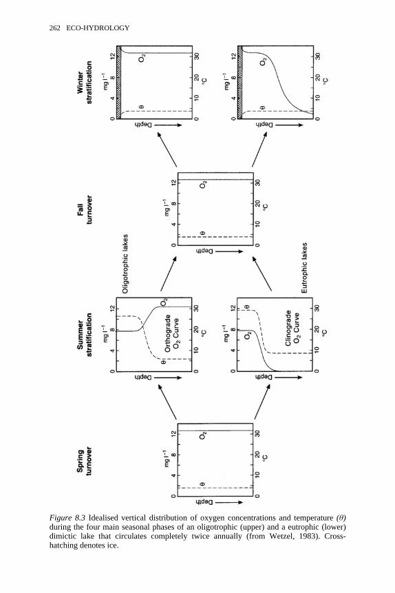
Figure 8.3 Idealised vertical distribution of oxygen concentrations and temperature (θ)during the four main seasonal phases of an oligotrophic (upper) and a eutrophic (lower)dimictic lake that circulates completely twice annually (from Wetzel, 1983). Cross-hatching denotes ice.
262 ECO-HYDROLOGY
and current generation in the receiving lake is also a function of discharge volumeof the river in relation to the volume of the lake or reservoir.
The theoretical retention time of a lake, given by total influents minusoutflows divided by the total volume of the lake, is realised only approximatelyin most lakes. Retention time varies with the dimensions and shape of the basin,seasonal rates of inflow, and stratification characteristics (Kajosaari, 1966). Athigh discharge rates, overflow and interflow of rivers may channel across orthrough the water mass of the stratified basin, whereas at lower discharge rates,river water may penetrate more into the main water mass and be mixed throughmore normal circulatory mechanisms. In larger lakes, geostrophic deflection ofincoming water, whether as surface flows or interflows, is consistently observed.Subaqueous spring or seepage waters flow similarly along density gradients,often through sediments and in littoral areas, where the nutrient concentrationsare often much greater than in the overlying waters. Comparative analyses of thehydrodynamics of river, reservoir and natural lake ecosystems emphasise thetransition from rapid, gravity-mediated, unidirectional (downstream) andhorizontal flushing in rivers to slow, wind-driven, relatively constant, three-dimensional movements in lakes (Wetzel, in press; see also the discussion ofthree-dimensional water exchanges in river systems in Chapter 7).
Water movements in lakes are often caused principally by wind, whichtransfers energy to the water. Rhythmic motions (oscillations) due to wind resultboth at the surface of the water and internally deep within the basin (Wetzel,1983; Imberger and Patterson, 1990). These motions and their attendant currentsmay be in phase or in opposition. The ultimate fate of these movements is todegrade into arrhythmic turbulent motions, which disperse the water as well aschemicals and organisms within it. These wind-mediated water movements areexceedingly important for nutrient cycling and biotic metabolism within lakes.Although properties such as density of planktonic organisms or concentrations ofdissolved organic matter could modify thermal conditions and influenceevaporation, stratification and related mixing processes, the organisms of theopen-water pelagic zone of lakes are of relatively minor consequence to thehydrology of lake basins per se.
The stratification and hydrological mixing patterns of course affect thedistribution and availability of nutrients, which in turn affect the levels of bioticproductivity of the lake ecosystems. Some of the couplings of nutrientdistributions are direct, such as importation to the surface waters of the photiczone with alteration of conditions essential for photosynthetic production oforganic matter. Other effects are indirect, such as alterations of oxygenconcentrations in stratified waters, which can result in marked changes in nutrientavailability to biota as redox conditions fluctuate. Space here does not allowdevelopment of these relationships; interested readers are referred to detailedsyntheses such as Hutchinson (1957) and Wetzel (1983).
Wind-mediated water movements can influence basin morphology and thesediments needed for colonisation of floating-leaved and emergent macrophytes.
PLANTS AND WATER IN AND ADJACENT TO LAKES 263
Lundqvist (1927) separated lakes into ‘littoral’ versus ‘profundal’ based on theirgeomorphology, rates of sediment formation and sites for colonisation by littoralmacrophytes. For example, the colonisation and development of macrophytes ismarkedly greater within protected littoral regions of lakes in the leeward side ofprevailing wind-induced wave turbulence in comparison with development alongopposing wave-swept regions of lakes (e.g. Gessner, 1959; Rich et al., 1971).Encroaching wetland vegetation, particularly emergent macrophytes, in littoralareas of lakes severely reduces water movement from wave-induced currents. Asa result, coarse and fine detrital particles of organic matter accumulate above andbelow the lake boundary. This rapid accrual of coarse organic detritus results incompacted deposits, anaerobic conditions, and rates of decomposition that areslower than rates of deposition. These deposits allow rapid colonisation andexpansion of emergent macrophytes in a lakeward direction in an acceleratingmanner over periods of years (Wetzel, 1979; Godshalk and Wetzel, 1984).
In littoral areas affected by prevailing wave action, colonisation andestablishment of macrophytes is reduced. Detrital particles from dead plants arerendered smaller during relatively rapid decay under conducive conditions insediments of moderate temperature and high dissolved oxygen (Godshalk andWetzel, 1978). Surficial materials that are deposited in these regions arefrequently resuspended by movements of surface waters, and ultimatelytransported to the central depression of the lake. Deeper littoral areas (e.g. <1–2m) are often colonised by submerged vascular plants and are less subject tosurface-water currents, which tend to remove residues. Sediment accretioncontinues until decreasing depths of c. 1 m from the surface are approached inmost small lakes. At that point, the water movements of wave action caneffectively displace and transport sediment deposits to the central basin. In somelakes, submerged macrophytes growing in shallow areas can accelerate sedimentaccretion. Where basin geomorphology has formed irregular raised lake basinareas within the photic zone that can support submerged macrophytes,sedimentation can accelerate in mounded areas (‘lake mounts’). Sediments inexposed areas, however, accrete only to within approximately 1 m of the watersurface, after which surface water movements resuspend sediments and dispersethem laterally to deeper areas. In a lake in northeast Indiana, USA, for example,no appreciable sediment accumulation occurred on exposed lake-mount littoralareas for over two millennia (Wetzel, 1970). Therefore, water movements inlakes cause various zones of the lake bottom to be subjected to erosional anddepositional processes. Water movements and gravitational force act in concertto cause a net movement of fine suspended detrital particles to the deepestportion of the lake. Such heterogeneity can affect the rates of biotically mediatedevapotranspiration and water losses (see ‘plants as controls on lake hydrologicalprocesses’, below).
Development of emergent and floating-leaved rooted macrophytes is furtherenhanced by the presence of nutrients in the sediments. The effect of sedimentson nutrient accumulation and availability can be illustrated by comparing two
264 ECO-HYDROLOGY
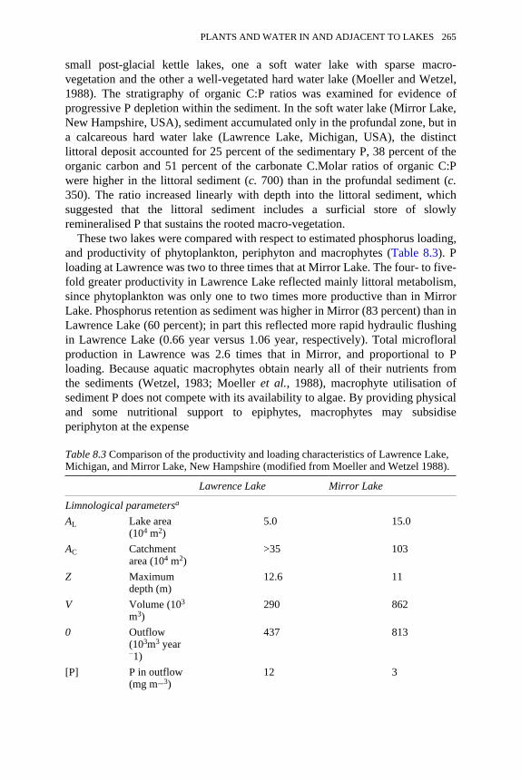
small post-glacial kettle lakes, one a soft water lake with sparse macro-vegetation and the other a well-vegetated hard water lake (Moeller and Wetzel,1988). The stratigraphy of organic C:P ratios was examined for evidence ofprogressive P depletion within the sediment. In the soft water lake (Mirror Lake,New Hampshire, USA), sediment accumulated only in the profundal zone, but ina calcareous hard water lake (Lawrence Lake, Michigan, USA), the distinctlittoral deposit accounted for 25 percent of the sedimentary P, 38 percent of theorganic carbon and 51 percent of the carbonate C.Molar ratios of organic C:Pwere higher in the littoral sediment (c. 700) than in the profundal sediment (c.350). The ratio increased linearly with depth into the littoral sediment, whichsuggested that the littoral sediment includes a surficial store of slowlyremineralised P that sustains the rooted macro-vegetation.
These two lakes were compared with respect to estimated phosphorus loading,and productivity of phytoplankton, periphyton and macrophytes (Table 8.3). Ploading at Lawrence was two to three times that at Mirror Lake. The four- to five-fold greater productivity in Lawrence Lake reflected mainly littoral metabolism,since phytoplankton was only one to two times more productive than in MirrorLake. Phosphorus retention as sediment was higher in Mirror (83 percent) than inLawrence Lake (60 percent); in part this reflected more rapid hydraulic flushingin Lawrence Lake (0.66 year versus 1.06 year, respectively). Total microfloralproduction in Lawrence was 2.6 times that in Mirror, and proportional to Ploading. Because aquatic macrophytes obtain nearly all of their nutrients fromthe sediments (Wetzel, 1983; Moeller et al., 1988), macrophyte utilisation ofsediment P does not compete with its availability to algae. By providing physicaland some nutritional support to epiphytes, macrophytes may subsidiseperiphyton at the expense
Table 8.3 Comparison of the productivity and loading characteristics of Lawrence Lake,Michigan, and Mirror Lake, New Hampshire (modified from Moeller and Wetzel 1988).
Lawrence Lake Mirror Lake
Limnological parametersa
AL Lake area(104 m2)
5.0 15.0
AC Catchmentarea (104 m2)
>35 103
Z Maximumdepth (m)
12.6 11
V Volume (103
m3)290 862
0 Outflow(103m3 year−1)
437 813
[P] P in outflow(mg m−3)
12 3
PLANTS AND WATER IN AND ADJACENT TO LAKES 265
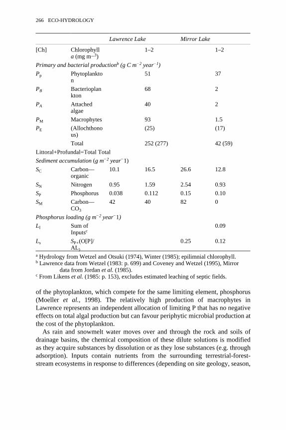
Lawrence Lake Mirror Lake
[Ch] Chlorophylla (mg m−3)
1–2 1–2
Primary and bacterial productionb (g C m−2 year−1)Pp Phytoplankto
n51 37
PB Bacterioplankton
68 2
PA Attachedalgae
40 2
PM Macrophytes 93 1.5PE (Allochthono
us)(25) (17)
Total 252 (277) 42 (59)Littoral+Profundal=Total TotalSediment accumulation (g m−2 year−1)SC Carbon—
organic10.1 16.5 26.6 12.8
SN Nitrogen 0.95 1.59 2.54 0.93SP Phosphorus 0.038 0.112 0.15 0.10SM Carbon—
CO3
42 40 82 0
Phosphorus loading (g m−2 year−1)LI Sum of
Inputsc0.09
Ls SP+(O[P]/AL)
0.25 0.12
a Hydrology from Wetzel and Otsuki (1974), Winter (1985); epilimnial chlorophyll.b Lawrence data from Wetzel (1983: p. 699) and Coveney and Wetzel (1995), Mirror
data from Jordan et al. (1985).c From Likens et al. (1985: p. 153), excludes estimated leaching of septic fields.
of the phytoplankton, which compete for the same limiting element, phosphorus(Moeller et al., 1998). The relatively high production of macrophytes inLawrence represents an independent allocation of limiting P that has no negativeeffects on total algal production but can favour periphytic microbial production atthe cost of the phytoplankton.
As rain and snowmelt water moves over and through the rock and soils ofdrainage basins, the chemical composition of these dilute solutions is modifiedas they acquire substances by dissolution or as they lose substances (e.g. throughadsorption). Inputs contain nutrients from the surrounding terrestrial-forest-stream ecosystems in response to differences (depending on site geology, season,
266 ECO-HYDROLOGY
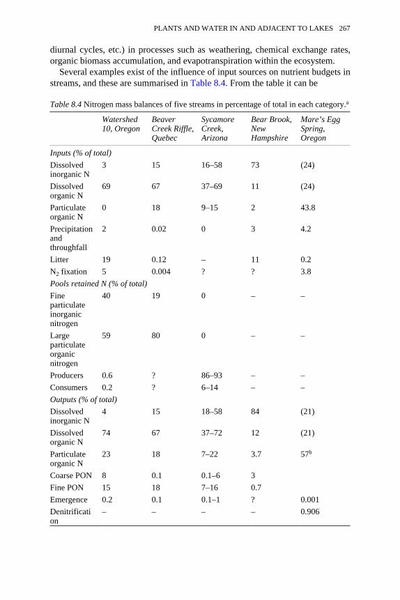
diurnal cycles, etc.) in processes such as weathering, chemical exchange rates,organic biomass accumulation, and evapotranspiration within the ecosystem.
Several examples exist of the influence of input sources on nutrient budgets instreams, and these are summarised in Table 8.4. From the table it can be
Table 8.4 Nitrogen mass balances of five streams in percentage of total in each category.a
Watershed10, Oregon
BeaverCreek Riffle,Quebec
SycamoreCreek,Arizona
Bear Brook,NewHampshire
Mare’s EggSpring,Oregon
Inputs (% of total)Dissolvedinorganic N
3 15 16–58 73 (24)
Dissolvedorganic N
69 67 37–69 11 (24)
Particulateorganic N
0 18 9–15 2 43.8
Precipitationandthroughfall
2 0.02 0 3 4.2
Litter 19 0.12 – 11 0.2N2 fixation 5 0.004 ? ? 3.8Pools retained N (% of total)Fineparticulateinorganicnitrogen
40 19 0 – –
Largeparticulateorganicnitrogen
59 80 0 – –
Producers 0.6 ? 86–93 – –Consumers 0.2 ? 6–14 – –Outputs (% of total)Dissolvedinorganic N
4 15 18–58 84 (21)
Dissolvedorganic N
74 67 37–72 12 (21)
Particulateorganic N
23 18 7–22 3.7 57b
Coarse PON 8 0.1 0.1–6 3Fine PON 15 18 7–16 0.7Emergence 0.2 0.1 0.1–1 ? 0.001Denitrification
– – – – 0.906
PLANTS AND WATER IN AND ADJACENT TO LAKES 267
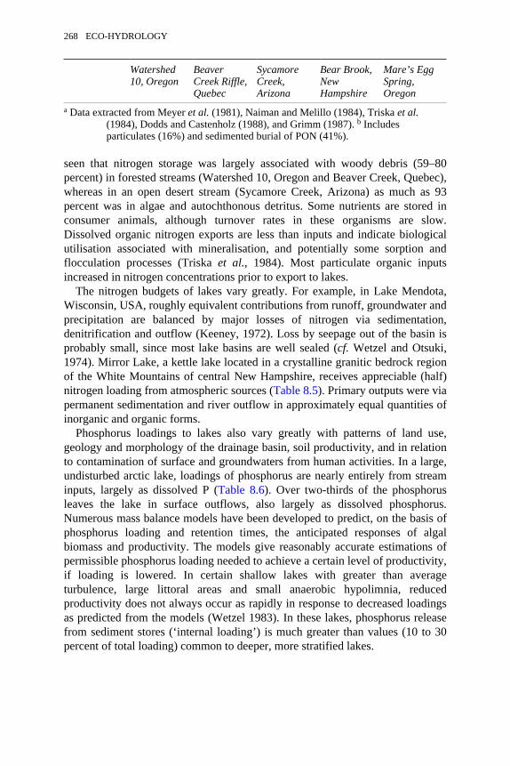
Watershed10, Oregon
BeaverCreek Riffle,Quebec
SycamoreCreek,Arizona
Bear Brook,NewHampshire
Mare’s EggSpring,Oregon
a Data extracted from Meyer et al. (1981), Naiman and Melillo (1984), Triska et al.(1984), Dodds and Castenholz (1988), and Grimm (1987). b Includesparticulates (16%) and sedimented burial of PON (41%).
seen that nitrogen storage was largely associated with woody debris (59–80percent) in forested streams (Watershed 10, Oregon and Beaver Creek, Quebec),whereas in an open desert stream (Sycamore Creek, Arizona) as much as 93percent was in algae and autochthonous detritus. Some nutrients are stored inconsumer animals, although turnover rates in these organisms are slow.Dissolved organic nitrogen exports are less than inputs and indicate biologicalutilisation associated with mineralisation, and potentially some sorption andflocculation processes (Triska et al., 1984). Most particulate organic inputsincreased in nitrogen concentrations prior to export to lakes.
The nitrogen budgets of lakes vary greatly. For example, in Lake Mendota,Wisconsin, USA, roughly equivalent contributions from runoff, groundwater andprecipitation are balanced by major losses of nitrogen via sedimentation,denitrification and outflow (Keeney, 1972). Loss by seepage out of the basin isprobably small, since most lake basins are well sealed (cf. Wetzel and Otsuki,1974). Mirror Lake, a kettle lake located in a crystalline granitic bedrock regionof the White Mountains of central New Hampshire, receives appreciable (half)nitrogen loading from atmospheric sources (Table 8.5). Primary outputs were viapermanent sedimentation and river outflow in approximately equal quantities ofinorganic and organic forms.
Phosphorus loadings to lakes also vary greatly with patterns of land use,geology and morphology of the drainage basin, soil productivity, and in relationto contamination of surface and groundwaters from human activities. In a large,undisturbed arctic lake, loadings of phosphorus are nearly entirely from streaminputs, largely as dissolved P (Table 8.6). Over two-thirds of the phosphorusleaves the lake in surface outflows, also largely as dissolved phosphorus.Numerous mass balance models have been developed to predict, on the basis ofphosphorus loading and retention times, the anticipated responses of algalbiomass and productivity. The models give reasonably accurate estimations ofpermissible phosphorus loading needed to achieve a certain level of productivity,if loading is lowered. In certain shallow lakes with greater than averageturbulence, large littoral areas and small anaerobic hypolimnia, reducedproductivity does not always occur as rapidly in response to decreased loadingsas predicted from the models (Wetzel 1983). In these lakes, phosphorus releasefrom sediment stores (‘internal loading’) is much greater than values (10 to 30percent of total loading) common to deeper, more stratified lakes.
268 ECO-HYDROLOGY
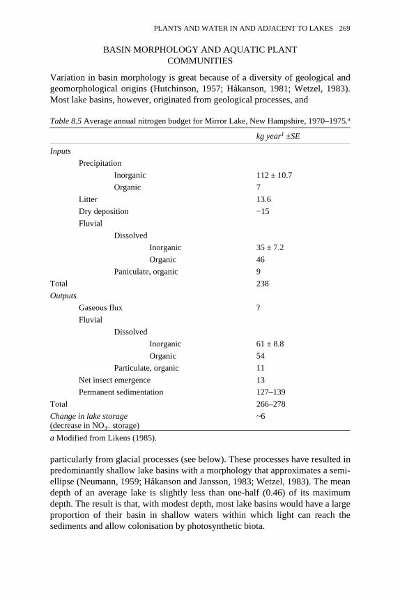
BASIN MORPHOLOGY AND AQUATIC PLANTCOMMUNITIES
Variation in basin morphology is great because of a diversity of geological andgeomorphological origins (Hutchinson, 1957; Håkanson, 1981; Wetzel, 1983).Most lake basins, however, originated from geological processes, and
Table 8.5 Average annual nitrogen budget for Mirror Lake, New Hampshire, 1970–1975.a
kg year1 ±SE
InputsPrecipitation
Inorganic 112 ± 10.7Organic 7
Litter 13.6Dry deposition −15Fluvial
DissolvedInorganic 35 ± 7.2Organic 46
Paniculate, organic 9Total 238Outputs
Gaseous flux ?Fluvial
DissolvedInorganic 61 ± 8.8Organic 54
Particulate, organic 11Net insect emergence 13Permanent sedimentation 127–139
Total 266–278Change in lake storage(decrease in NO3− storage)
~6
a Modified from Likens (1985).
particularly from glacial processes (see below). These processes have resulted inpredominantly shallow lake basins with a morphology that approximates a semi-ellipse (Neumann, 1959; Håkanson and Jansson, 1983; Wetzel, 1983). The meandepth of an average lake is slightly less than one-half (0.46) of its maximumdepth. The result is that, with modest depth, most lake basins would have a largeproportion of their basin in shallow waters within which light can reach thesediments and allow colonisation by photosynthetic biota.
PLANTS AND WATER IN AND ADJACENT TO LAKES 269
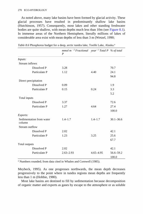
As noted above, many lake basins have been formed by glacial activity. Theseglacial processes have resulted in predominantly shallow lake basins(Hutchinson, 1957). Consequently, most lakes and other standing freshwaterbodies are quite shallow, with mean depths much less than 10m (see Figure 8.1).In immense areas of the Northern Hemisphere, literally millions of lakes ofconsiderable area exist with mean depths of less than 3 m (Wetzel, 1990;
Table 8.6 Phosphorus budget for a deep, arctic tundra lake, Toolik Lake, Alaska.a
mmol m −2 FractionalP
year−1 Total P % of total
Inputs:Stream inflows
Dissolved P 3.28 70.7Particulate P 1.12 4.40 24.1
94.8Direct precipitation
Dissolved P 0.09 1.9Particulate P 0.15 0.24 3.3
5.2Total inputs
Dissolved P 3.37 72.6Particulate P 1.27 4.64 27.4
100.0Exports:Sedimentation from watercolumn
1.4–1.7 1.4–1.7 30.1–36.6
Stream outflowDissolved P 2.02 42.1Particulate P 1.23 3.25 25.6
67.7Total outputs
Dissolved P 2.02 42.1Particulate P 2.63–2.93 4.65–4.95 56.6–59.2
100.0a Numbers rounded; from data cited in Whalen and Cornwell (1985).
Meybeck, 1995). As one progresses northwards, the mean depth decreasesprogressively to the point where in tundra regions mean depths are frequentlyless than 1 m (Hobbie, 1980).
Most lake basins are destined to fill by sedimentation because decompositionof organic matter and exports as gases by escape to the atmosphere or as soluble
270 ECO-HYDROLOGY

compounds with outflows are nearly always less than allochthonous loadings oforganic matter and clastic (minerogenic) sediments and autochthonous loadingsof organic matter. The rates of these loadings and sedimentation within the basinare dependent upon (1) the nutrient loadings from the catchment and (2) theinitial formation and long-term modifications to the basin morphometry bysedimentation. As sedimentation increases, a greater proportion of the basinsediments per se are brought into the photic zone and are available forcolonisation by the extremely productive littoral and wetland communitiesdiscussed above. Greater productivity of small, shallow lakes is directlycorrelated with higher water-sediment interface area per water volume (i.e. lowermean depth).
Sedimentation rates are directly coupled with littoral and wetlandproductivity. Because phytoplanktonic productivity is so low, as discussedearlier, autochthonous productivity by littoral and wetland aquatic plantsprovides a major source of organic matter to lakes. On a global basis, the littoralzone dominates over the pelagic (giving low P:L ratios among most standingwater ecosystems (Figure 8.4). Additions from the wetland components to thelittoral zone result in low ratios (P/[W+L]). A similar very low ratio is apparentamong rivers, because the floodplains are functioning as major wetland andlittoral components of most river ecosystems.
Most of the particulate organic matter produced in the wetland-littoralcomplex of lake ecosystems is deposited within the land-water interface regions(Wetzel, 1983; 1990; 1992). Decomposition is incomplete because of anaerobicchemical and metabolic conditions, which reduce the availability of electron-acceptor compounds and enhance the production of fermentative metabolicproducts. The structural plant tissues of most productive higher aquatic plants areincompletely decomposed and result in an accumulation of relatively recalcitrantorganic matter. Accumulation rates of sediments from higher plants is muchgreater than from planktonic sources. As a result, sedimentation rates are muchmore rapid in shallow areas. The process is self-reinforcing: as more sedimentsreach the photic zone, the productivity of higher aquatic plants accelerates(Wetzel, 1979).
As a greater proportion of the lake basins succeeds to littoral and wetlandvegetation, hydrological alterations by plant metabolism also occur. Not only isdirect evapotranspiration increased with greater littoral development, but theprogression is set forth towards a situation where losses from the basin willexceed additions.
PLANTS AS A CONTROL ON LAKE HYDROLOGICALPROCESSES
Evaporative losses from lakes are greatly modified by transpiration fromemergent and floating-leaved aquatic plants (cf. review of Gessner, 1959). Ratesof transpiration and evaporative losses to the atmosphere vary with an array of
PLANTS AND WATER IN AND ADJACENT TO LAKES 271
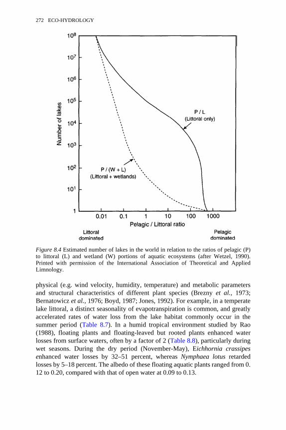
physical (e.g. wind velocity, humidity, temperature) and metabolic parametersand structural characteristics of different plant species (Brezny et al., 1973;Bernatowicz et al., 1976; Boyd, 1987; Jones, 1992). For example, in a temperatelake littoral, a distinct seasonality of evapotranspiration is common, and greatlyaccelerated rates of water loss from the lake habitat commonly occur in thesummer period (Table 8.7). In a humid tropical environment studied by Rao(1988), floating plants and floating-leaved but rooted plants enhanced waterlosses from surface waters, often by a factor of 2 (Table 8.8), particularly duringwet seasons. During the dry period (November-May), Eichhornia crassipesenhanced water losses by 32–51 percent, whereas Nymphaea lotus retardedlosses by 5–18 percent. The albedo of these floating aquatic plants ranged from 0.12 to 0.20, compared with that of open water at 0.09 to 0.13.
Figure 8.4 Estimated number of lakes in the world in relation to the ratios of pelagic (P)to littoral (L) and wetland (W) portions of aquatic ecosystems (after Wetzel, 1990).Printed with permission of the International Association of Theoretical and AppliedLimnology.
272 ECO-HYDROLOGY
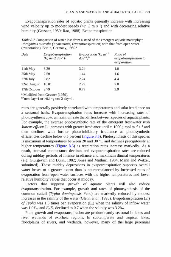
Evapotranspiration rates of aquatic plants generally increase with increasingwind velocity up to modest speeds (<c. 2 m s−1) and with decreasing relativehumidity (Gessner, 1959; Rao, 1988). Evapotranspiration
Table 8.7 Comparison of water loss from a stand of the emergent aquatic macrophytePhragmites australis (=communis) (evapotranspiration) with that from open water(evaporation), Berlin, Germany, 1950.a
Date Evapotranspiration(kg m−2 day−1)
Evaporation (kg m−2
day−1)bRatio ofevapotranspiration toevaporation
11th May 3.20 3.24 1.025th May 2.50 1.44 1.627th July 9.82 2.24 4.422nd August 16.01 2.29 7.017th October 2.79 0.79 3.9a Modified from Gessner (1959).b=mm day−1 or ×0.1=g cm−2 day−1.
rates are generally positively correlated with temperatures and solar irradiance ona seasonal basis. Evapotranspiration rates increase with increasing rates ofphotosynthesis up to a maximum rate that differs between species of aquatic plants.For example, the average photosynthetic rate of the emergent freshwater rushJuncus effusus L. increases with greater irradiance until c. 1000 µmol m−2 s−1 andthen declines with further photo-inhibitory irradiance as photosyntheticefficiencies decline below 0.5 percent (Figure 8.5). Photosynthesis of this speciesis maximum at temperatures between 20 and 30 °C and declines precipitously athigher temperatures (Figure 8.5) as respiration rates increase markedly. As aresult, stomatal conductance declines and evapotranspiration rates are reducedduring midday periods of intense irradiance and maximum diurnal temperatures(e.g. Giurgevich and Dunn, 1982; Jones and Muthuri, 1984; Mann and Wetzel,submitted). These midday depressions in evapotranspiration suppress overallwater losses to a greater extent than is counterbalanced by increased rates ofevaporation from open water surfaces with the higher temperatures and lowerrelative humidity values that occur at midday.
Factors that suppress growth of aquatic plants will also reduceevapotranspiration. For example, growth and rates of photosynthesis of thecommon cattail (Typha domingensis Pers.) are markedly reduced by modestincreases in the salinity of the water (Glenn et al., 1995). Evapotranspiration (Et)of Typha was 1.3 times pan evaporation (Eo) when the salinity of inflow waterwas 1.0‰, and Et/Eo declined to 0.7 when the salinity was 3.2‰.
Plant growth and evapotranspiration are predominantly seasonal in lakes andriver wetlands of exorheic regions. In subtemperate and tropical lakes,floodplains of rivers, and wetlands, however, many of the large perennial
PLANTS AND WATER IN AND ADJACENT TO LAKES 273
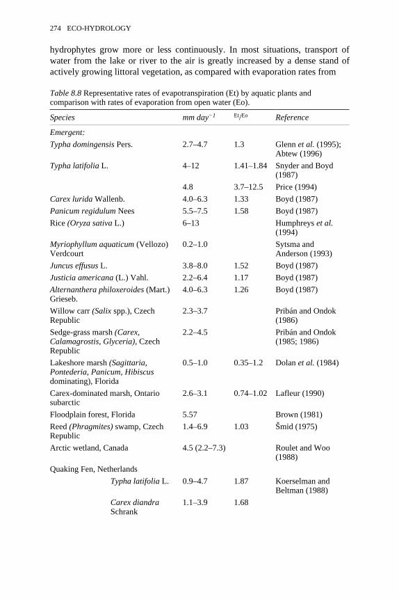
hydrophytes grow more or less continuously. In most situations, transport ofwater from the lake or river to the air is greatly increased by a dense stand ofactively growing littoral vegetation, as compared with evaporation rates from
Table 8.8 Representative rates of evapotranspiration (Et) by aquatic plants andcomparison with rates of evaporation from open water (Eo).
Species mm day−1 Et/Eo Reference
Emergent:Typha domingensis Pers. 2.7–4.7 1.3 Glenn et al. (1995);
Abtew (1996)Typha latifolia L. 4–12 1.41–1.84 Snyder and Boyd
(1987)4.8 3.7–12.5 Price (1994)
Carex lurida Wallenb. 4.0–6.3 1.33 Boyd (1987)Panicum regidulum Nees 5.5–7.5 1.58 Boyd (1987)Rice (Oryza sativa L.) 6–13 Humphreys et al.
(1994)Myriophyllum aquaticum (Vellozo)Verdcourt
0.2–1.0 Sytsma andAnderson (1993)
Juncus effusus L. 3.8–8.0 1.52 Boyd (1987)Justicia americana (L.) Vahl. 2.2–6.4 1.17 Boyd (1987)Alternanthera philoxeroides (Mart.)Grieseb.
4.0–6.3 1.26 Boyd (1987)
Willow carr (Salix spp.), CzechRepublic
2.3–3.7 Pribán and Ondok(1986)
Sedge-grass marsh (Carex,Calamagrostis, Glyceria), CzechRepublic
2.2–4.5 Pribán and Ondok(1985; 1986)
Lakeshore marsh (Sagittaria,Pontederia, Panicum, Hibiscusdominating), Florida
0.5–1.0 0.35–1.2 Dolan et al. (1984)
Carex-dominated marsh, Ontariosubarctic
2.6–3.1 0.74–1.02 Lafleur (1990)
Floodplain forest, Florida 5.57 Brown (1981)Reed (Phragmites) swamp, CzechRepublic
1.4–6.9 1.03 Šmid (1975)
Arctic wetland, Canada 4.5 (2.2–7.3) Roulet and Woo(1988)
Quaking Fen, NetherlandsTypha latifolia L. 0.9–4.7 1.87 Koerselman and
Beltman (1988)Carex diandraSchrank
1.1–3.9 1.68
274 ECO-HYDROLOGY
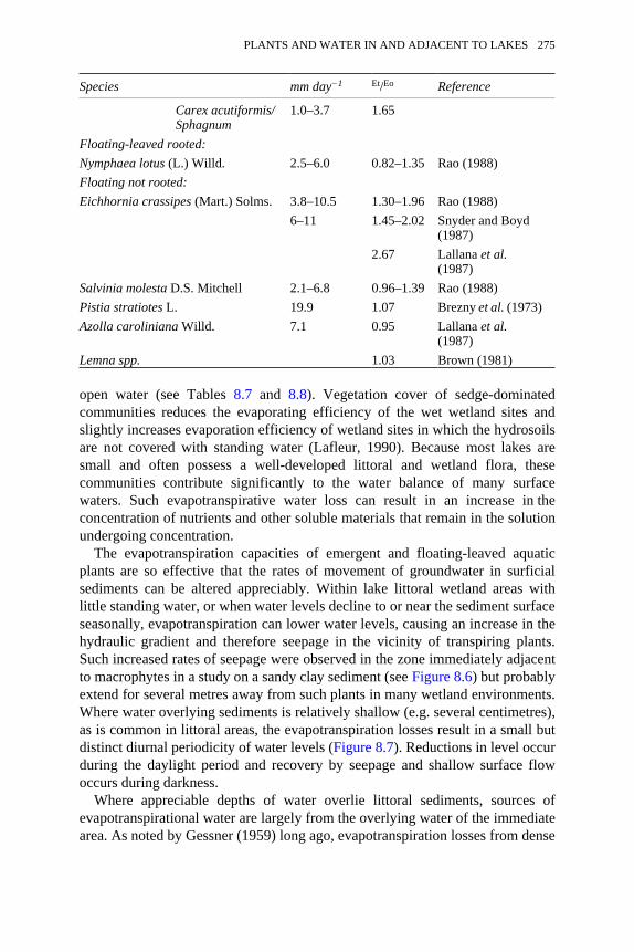
Species mm day−1 Et/Eo Reference
Carex acutiformis/Sphagnum
1.0–3.7 1.65
Floating-leaved rooted:Nymphaea lotus (L.) Willd. 2.5–6.0 0.82–1.35 Rao (1988)Floating not rooted:Eichhornia crassipes (Mart.) Solms. 3.8–10.5 1.30–1.96 Rao (1988)
6–11 1.45–2.02 Snyder and Boyd(1987)
2.67 Lallana et al.(1987)
Salvinia molesta D.S. Mitchell 2.1–6.8 0.96–1.39 Rao (1988)Pistia stratiotes L. 19.9 1.07 Brezny et al. (1973)Azolla caroliniana Willd. 7.1 0.95 Lallana et al.
(1987)Lemna spp. 1.03 Brown (1981)
open water (see Tables 8.7 and 8.8). Vegetation cover of sedge-dominatedcommunities reduces the evaporating efficiency of the wet wetland sites andslightly increases evaporation efficiency of wetland sites in which the hydrosoilsare not covered with standing water (Lafleur, 1990). Because most lakes aresmall and often possess a well-developed littoral and wetland flora, thesecommunities contribute significantly to the water balance of many surfacewaters. Such evapotranspirative water loss can result in an increase in theconcentration of nutrients and other soluble materials that remain in the solutionundergoing concentration.
The evapotranspiration capacities of emergent and floating-leaved aquaticplants are so effective that the rates of movement of groundwater in surficialsediments can be altered appreciably. Within lake littoral wetland areas withlittle standing water, or when water levels decline to or near the sediment surfaceseasonally, evapotranspiration can lower water levels, causing an increase in thehydraulic gradient and therefore seepage in the vicinity of transpiring plants.Such increased rates of seepage were observed in the zone immediately adjacentto macrophytes in a study on a sandy clay sediment (see Figure 8.6) but probablyextend for several metres away from such plants in many wetland environments.Where water overlying sediments is relatively shallow (e.g. several centimetres),as is common in littoral areas, the evapotranspiration losses result in a small butdistinct diurnal periodicity of water levels (Figure 8.7). Reductions in level occurduring the daylight period and recovery by seepage and shallow surface flowoccurs during darkness.
Where appreciable depths of water overlie littoral sediments, sources ofevapotranspirational water are largely from the overlying water of the immediatearea. As noted by Gessner (1959) long ago, evapotranspiration losses from dense
PLANTS AND WATER IN AND ADJACENT TO LAKES 275
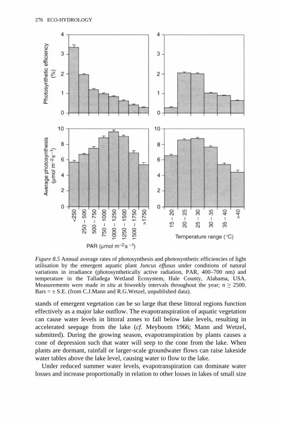
stands of emergent vegetation can be so large that these littoral regions functioneffectively as a major lake outflow. The evapotranspiration of aquatic vegetationcan cause water levels in littoral zones to fall below lake levels, resulting inaccelerated seepage from the lake (cf. Meyboom 1966; Mann and Wetzel,submitted). During the growing season, evapotranspiration by plants causes acone of depression such that water will seep to the cone from the lake. Whenplants are dormant, rainfall or larger-scale groundwater flows can raise lakesidewater tables above the lake level, causing water to flow to the lake.
Under reduced summer water levels, evapotranspiration can dominate waterlosses and increase proportionally in relation to other losses in lakes of small size
Figure 8.5 Annual average rates of photosynthesis and photosynthetic efficiencies of lightutilisation by the emergent aquatic plant Juncus effusus under conditions of naturalvariations in irradiance (photosynthetically active radiation, PAR, 400–700 nm) andtemperature in the Talladega Wetland Ecosystem, Hale County, Alabama, USA.Measurements were made in situ at biweekly intervals throughout the year; n ≥ 2500.Bars = ± S.E. (from C.J.Mann and R.G.Wetzel, unpublished data).
276 ECO-HYDROLOGY
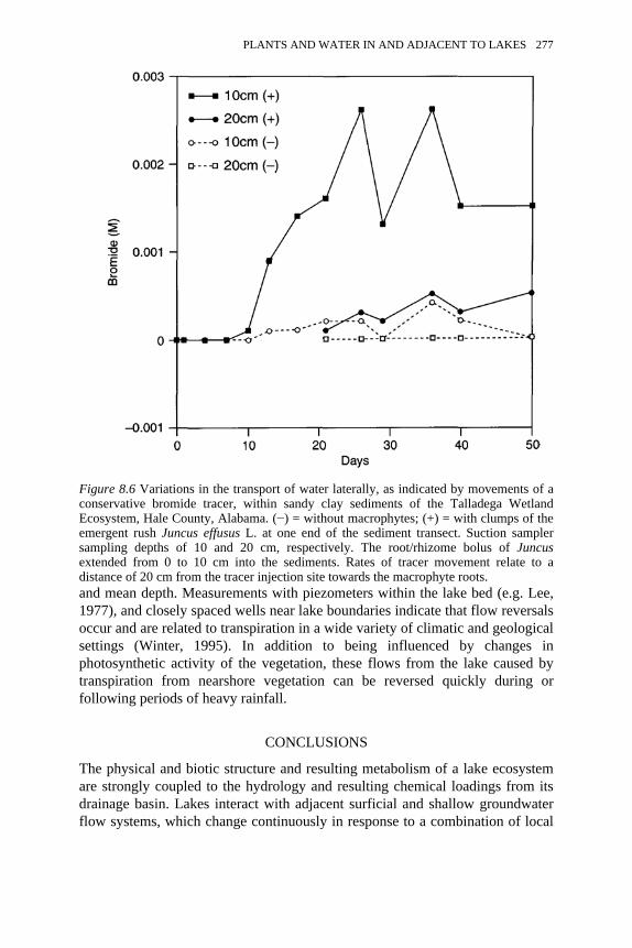
and mean depth. Measurements with piezometers within the lake bed (e.g. Lee,1977), and closely spaced wells near lake boundaries indicate that flow reversalsoccur and are related to transpiration in a wide variety of climatic and geologicalsettings (Winter, 1995). In addition to being influenced by changes inphotosynthetic activity of the vegetation, these flows from the lake caused bytranspiration from nearshore vegetation can be reversed quickly during orfollowing periods of heavy rainfall.
CONCLUSIONS
The physical and biotic structure and resulting metabolism of a lake ecosystemare strongly coupled to the hydrology and resulting chemical loadings from itsdrainage basin. Lakes interact with adjacent surficial and shallow groundwaterflow systems, which change continuously in response to a combination of local
Figure 8.6 Variations in the transport of water laterally, as indicated by movements of aconservative bromide tracer, within sandy clay sediments of the Talladega WetlandEcosystem, Hale County, Alabama. (−) = without macrophytes; (+) = with clumps of theemergent rush Juncus effusus L. at one end of the sediment transect. Suction samplersampling depths of 10 and 20 cm, respectively. The root/rhizome bolus of Juncusextended from 0 to 10 cm into the sediments. Rates of tracer movement relate to adistance of 20 cm from the tracer injection site towards the macrophyte roots.
PLANTS AND WATER IN AND ADJACENT TO LAKES 277
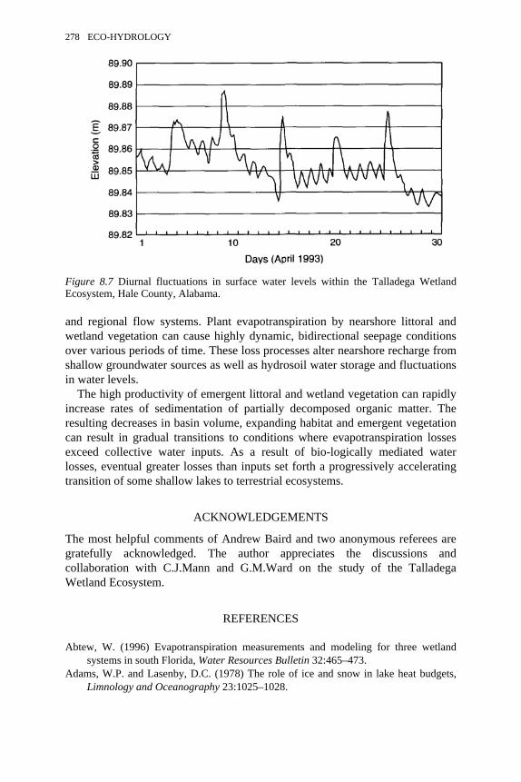
and regional flow systems. Plant evapotranspiration by nearshore littoral andwetland vegetation can cause highly dynamic, bidirectional seepage conditionsover various periods of time. These loss processes alter nearshore recharge fromshallow groundwater sources as well as hydrosoil water storage and fluctuationsin water levels.
The high productivity of emergent littoral and wetland vegetation can rapidlyincrease rates of sedimentation of partially decomposed organic matter. Theresulting decreases in basin volume, expanding habitat and emergent vegetationcan result in gradual transitions to conditions where evapotranspiration lossesexceed collective water inputs. As a result of bio-logically mediated waterlosses, eventual greater losses than inputs set forth a progressively acceleratingtransition of some shallow lakes to terrestrial ecosystems.
ACKNOWLEDGEMENTS
The most helpful comments of Andrew Baird and two anonymous referees aregratefully acknowledged. The author appreciates the discussions andcollaboration with C.J.Mann and G.M.Ward on the study of the TalladegaWetland Ecosystem.
REFERENCES
Abtew, W. (1996) Evapotranspiration measurements and modeling for three wetlandsystems in south Florida, Water Resources Bulletin 32:465–473.
Adams, W.P. and Lasenby, D.C. (1978) The role of ice and snow in lake heat budgets,Limnology and Oceanography 23:1025–1028.
Figure 8.7 Diurnal fluctuations in surface water levels within the Talladega WetlandEcosystem, Hale County, Alabama.
278 ECO-HYDROLOGY
Bernatowicz, S., Leszczynski, S. and Tyczynska, S. (1976) The influence of transpirationby emergent plants on the water balance in lakes, Aquatic Botany 2: 275–288.
Boyd, C.E. (1987) Evapotranspiration/evaporation (E/Eo) ratios for aquatic plants,Journal of Aquatic Plant Management 25:1–3.
Brezny, O., Metha, I. and Sharma, R.K. (1973) Studies on the evapotranspiration of someaquatic weeds, Weed Science 21:197–204.
Brown, S. (1981) A comparison of the structure, primary productivity, and transpirationof cypress ecosystems in Florida, Ecological Monographs 51:403–427.
Brutsaert, W.H. (1982) Evaporation into the Atmosphere, Dordrecht: Reidel, 299 pp.Carter, S.M., Ward, G.M., Wetzel, R.G. and Benke, A.C. (in press) Growth, production,
and senescence of Nymphaea odorata Aiton in a southeastern (U.S.A.) wetland,Aquatic Botany.
Coveney, M.F. and Wetzel, R.G. (1995) Biomass, production, and specific growth rate ofbacterioplankton and coupling to phytoplankton in an oligotrophic lake, Limnologyand Oceanography 40:1187–1200.
Dodds, W.K. and Castenholz, R.W. (1988) The nitrogen budget of an oligotrophic coldwater pond, Archiv für Hydrobiologie/Supplement 79:343–362.
Dolan, T.J., Hermann, A.J., Bayley, S.E. and Zoltek, J., Jr (1984) Evapotranspiration of aFlorida, U.S.A., freshwater wetland, Journal of Hydrology 74:355–371.
Gessner, F. (1959) Hydrobotanik. II. Stoffhaushalt, Berlin: VEB Deutscher Verlag derWissenschaften, Berlin, 701 pp.
Giurgevich, J.R. and Dunn, E.L. (1982) Seasonal patterns of daily net photosynthesis,transpiration and net primary productivity of Juncus roemerianus and Spartinaalterniflora in a Georgia salt marsh, Oecologia 52:404–410.
Glenn, E., Thompson, T.L., Frye, R., Riley, J. and Baumgartner, D. (1995) Effects ofsalinity on growth and evapotranspiration of Typha domingensis Pers., AquaticBotany 52:75–91.
Godshalk, G.L. and Wetzel, R.G. (1978) Decomposition of aquatic angiosperms. II.Particulate components, Aquatic Botany 5:301–328.
Godshalk, G.L. and Wetzel, R.G. (1984) Accumulation of sediment organic matter in ahardwater lake with reference to lake ontogeny, Bulletin of Marine Science 35:576–586.
Grimm, N.B. (1987) Nitrogen dynamics during succession in a desert stream, Ecology 68:1157–1170.
Håkanson, L. (1981) A Manual of Lake Morphometry, New York: Springer-Verlag, 78pp.Håkanson, L. and Jansson, M. (1983) Principles of Lake Sedimentology, New York:
Springer-Verlag, 316 pp.Hobbie, J.E. (ed.) (1980) Limnology of Tundra Ponds, Stroudsburg: Hutchinson and Ross
Inc., 514 pp.Hostetler, S.W. (1995) Hydrological and thermal response of lakes to climate: description
and modeling, in A.Lerman, D.M.Imboden, and J.R.Gat (eds) Physics and Chemistryof Lakes, Berlin: Springer-Verlag, pp. 63–82.
Humphreys, E., Meyer, W.S., Prathapar, S.A. and Smith, D.J. (1994) Estimation ofevapotranspiration from rice in southern New South Wales: a review, AustralianJournal of Experimental Agriculture 34:1069–1078.
Hutchinson, G.E. (1957) A Treatise on Limnology. I. Geography, Physics, andChemistry, New York: Wiley, 1015 pp.
PLANTS AND WATER IN AND ADJACENT TO LAKES 279
Hutchinson, G.E. (1975) A Treatise on Limnology. III. Limnological Botany, New York:Wiley, 660 pp.
Imberger, J. and Patterson, J.C. (1990) Physical limnology, Advances of AppliedMechanics 27:303–475.
Imboden, D.M. and Wuest, A. (1995) Mixing mechanisms in lakes, in A.Lerman,D.M.Imboden, and J.R.Gat (eds) Physics and Chemistry of Lakes, Berlin: Springer-Verlag, pp. 83–138.
Jones, F.E. (1992) Evaporation of Water With Emphasis on Applications andMeasurements, Chelsea, Michigan: Lewis, 188 pp.
Jones, M.B. and Muthuri, F.M. (1984) The diurnal course of plant water potential,stomatal conductance and transpiration in a papyrus (Cyperus papyrus L.) canopy,Oecologia 63:252–255.
Jordan, M.J., Likens, G.E. and Peterson, B.J. (1985) Mirror Lake—Biologicconsiderations. C. Organic carbon budget, in G.E.Likens (ed.) An EcosystemApproach to Aquatic Ecology: Mirror Lake and its Environment, New York:Springer-Verlag, pp. 292–301.
Kajosaari, E. (1966) Estimation of the detention period of a lake, VerhandlungenInternationale Vereinigung der Limnologie 16:139–143.
Keeney, D.R. (1972) The Fate of Nitrogen in Aquatic Ecosystems. Literature Review 3,Water Resources Center, University of Wisconsin, 59 pp.
Kilham, S.S. and Kilham, P. (1990) Tropical limnology: do African lakes violate the ‘firstlaw’ of limnology? Verhandlungen Internationale Vereinigung der Limnologie 24:68–72.
Koerselman, W. and Beltman, B. (1988) Evapotranspiration from fens in relation toPenman’s potential free water evaporation (Eo) and pan evaporation, Aquatic Botany31:307–320.
Lafleur, P.M. (1990) Evapotranspiration from sedge-dominated wetland surfaces, AquaticBotany 37:341–353.
Lallana, V.H., Sabattini, R.A. and Lallana, M.C. (1987) Evapotranspiration fromEichhornia crassipes, Pistia stratiotes, Salvinia herzogii and Azolla carolinianaduring summer in Argentina , Journal of Aquatic Plant Management 25:48–50.
Lee, D.R. (1977) A device for measuring seepage flux in lakes and estuaries, Limnologyand Oceanography 22:155–163.
Lee, D.R. (1985) Method for locating sediment anomalies in lakebeds that can be causedby groundwater flow, Journal of Hydrology 79:187–193.
Lee, D.R. and Cherry, J.A. (1978) A field exercise on groundwater flow using seepagemeters and mini-piezometers, Journal of Geological Education 27: 6–10.
Lee, D.R. and Harvey, F.E. (1996) Installing piezometers in deepwater sediments, WaterResources Research 32:1113–1117.
Likens, G.E. (1984) Beyond the shoreline: A watershed-ecosystem approach,Verhandlungen Internationale Vereinigung der Limnologie 22:1–22.
Likens, G.E. (ed.) (1985) An Ecosystem Approach to Aquatic Ecology: Mirror Lake andits Environment, New York: Springer-Verlag, 516 pp.
Likens, G.E., Bormann, F.H., Pierce, R.S., Eaton, J.S. and Johnson, N.M. (1977)Biogeochemistry of a Forested Ecosystem, New York: Springer-Verlag, 146 pp.
Likens, G.E., Eaton, J.S., Johnson, N.M., and Pierce, R.S. (1985) Flux and balance ofwater and chemicals, in G.E.Likens (ed.), An Ecosystem Approach to Aquatic
280 ECO-HYDROLOGY
Ecology: Mirror Lake and Its Environment, New York: Springer-Verlag,pp. 135–155.
Lundqvist, G. (1927) Bodenablagerungen und Entwicklungstypen der Seen, DieBinnengewässer 2:1–122.
Mann, C.J. and Wetzel, R.G. (submitted) Hydrology and subsurface water flows in awetland ecosystem, Wetland Ecology and Management.
Mason, I.M., Guzkowska, M.A.J. and Rapley, C.G. (1994) The response of lake levelsand areas to climatic change, Climatic Change 27:161–197.
Meybeck, M. (1995) Global distribution of lakes, in A.Lerman, D.M.Imboden, andJ.R.Gat (eds) Physics and Chemistry of Lakes, Berlin: Springer-Verlag, pp. 1–35.
Meyboom, P. (1966) Unsteady groundwater flow near a willow ring in hummockymoraine , Journal of Hydrology 4:38–62.
Meyer, J.L., Likens, G.E. and Sloane, J. (1981) Phosphorus, nitrogen, and organic carbonflux in a headwater stream, Archiv für Hydrobiologie 91:28–44.
Moeller, R.E. and Wetzel, R.G. (1988) Littoral vs profundal components of sedimentaccumulation: contrasting roles as phosphorus sinks, Verhandlungen InternationaleVereinigung der Limnologie 23:386–393.
Moeller, R.G., Burkholder, J.M. and Wetzel, R.G. (1988) Significance of sedimentaryphosphorus to a submersed freshwater macrophyte (Najas flexilis) and its algalepiphytes, Aquatic Botany 32:261–281.
Moeller, R.E., Wetzel, R.G. and Osenberg, C.W. (1998) Concordance of phosphoruslimitation in lakes: bacterioplankton, phytoplankton, epiphyte-snail consumers, androoted macrophytes, in E.Jeppesen, Ma. Søndergaard, Mo. Søndergaard andK.Christoffersen (eds) The Structuring Role of Submersed Macrophytes in Lakes,Berlin: Springer-Verlag, pp. 318–325.
Naiman, R.J. and Melillo, J.M. (1984) Nitrogen budget of a subarctic stream altered bybeaver (Castor canadensis), Oecologia 62:150–155.
Neumann, J. (1959) Maximum depth and average depth of lakes, Journal of FisheriesResearch Board of Canada 16:923–927.
Pribán, K. and J.P.Ondok, (1985) Heat balance components and evapotranspiration from asedge-grass marsh, Folia Geobotanica et Phytotaxonomica Praha 20:41–56.
Pribán, K. and Ondok, J.P. (1986) Evapotranspiration of a willow carr in summer, AquaticBotany 25:203–216.
Price, J.S. (1994) Evapotranspiration from a lakeshore Typha marsh on Lake Ontario,Aquatic Botany 48:261–272.
Rao, A.S. (1988) Evapotranspiration rates of Eichhornia crassipes (Mart.) Solms, Salviniamolesta D.S.Mitchell and Nymphaea lotus (L.) Willd. Linn, in a humid tropicalclimate, Aquatic Botany 30:215–222.
Rich, P.H., Wetzel, R.G. and Thuy, N.V. (1971) Distribution, production and role ofaquatic macrophytes in a southern Michigan marl lake, Freshwater Biology 1: 3–21.
Roulet, N.T. and Woo, M. (1988) Wetland and lake evaporation in the low Arctic, Arcticand Alpine Research 18:195–200.
Sculthorpe, C.D. (1967) The Biology of Aquatic Vascular Plants, New York: St Martin’sPress, 610 pp.
Serruya, C. and Pollinger, U. (1984) Lakes of the Warm Belt, Cambridge: CambridgeUniversity Press, 569 pp.
PLANTS AND WATER IN AND ADJACENT TO LAKES 281
Shaw, R.D. and Prepas, E.E. (1990) Groundwater-lake interactions. 2. Nearshore seepagepatterns and the contribution of groundwater to lakes in central Alberta, Journal ofHydrology 119:121–136.
Smid, P. (1975) Evaporation from a reedswamp, Journal of Ecology 66:299–309.Snyder, R.L. and Boyd, C.E. (1987) Evapotranspiration by Eichhorina crassipes (Mart.)
Solms and Typha latifolia L., Aquatic Botany 27:217–227.Street, F.A. (1980) The relative importance of climate and local hydrogeological factors in
influencing lake level fluctuations, Palaeoecology of Africa 12:137–158.Sturrock, A.M., Winter, T.C. and Rosenberry, D.O. (1992) Energy budget evaporation
from Williams Lake: a closed lake in north central Minnesota, Water ResourcesResearch 28:1605–1617.
Sytsma, M.D. and Anderson, L.W.J. (1993) Transpiration by an emergent macrophyte:Source of water and implications for nutrient supply, Hydrobiologia 271: 97–108.
Szesztay, K. (1974) Water balance and water level fluctuations of lakes, HydrologicalSciences Bulletin 19:74–84.
Triska, F.J., Sedell, J.R., Cromack, K., Jr, Gregory, S.V. and McCorison, F.M. (1984)Nitrogen budget for a small coniferous forest stream, Ecological Monographs 54:119–140.
Westlake, D.F. (1963) Comparisons of plant productivity, Biological Reviews 38:385–425.
Westlake, D.F. (1965) Some basic data for investigations of the productivity of aquaticmacrophytes, Memorie dell’Istituto Italiano di Idrobiologia 18 (supplement):229–248.
Wetzel, R.G. (1965) Nutritional aspects of algal productivity in marl lakes with particularreference to enrichment bioassays and their interpretation, Memorie dell’IstitutoItaliano di Idrobiologia 18 (supplement): 137–157.
Wetzel, R.G. (1966) Productivity and nutrient relationships in marl lakes of northernIndiana, Verhandlungen Internationale Vereinigung der Limnologie 16: 321–332.
Wetzel, R.G. (1970) Recent and post-glacial production rates of a marl lake, Limnologyand Oceanography 15:491–503.
Wetzel, R.G. (1979) The role of the littoral zone and detritus in lake metabolism, Archivfür Hydrobiologie Beiheft Ergebnisse Limnologie 13:145–161.
Wetzel, R.G. (1983) Limnology, 2nd edition, Philadelphia: Saunders College Publishing,860 pp.
Wetzel, R.G. (1990) Land-water interfaces: metabolic and limnological regulators,Verhandlungen Internationale Vereinigung der Limnologie 24:6–24.
Wetzel, R.G. (1991) Extracellular enzymatic interactions in aquatic ecosystems: storage,redistribution, and interspecific communication, in R.J.Chróst (ed.) MicrobialEnzymes in Aquatic Environments, New York: Springer-Verlag, pp. 6–28.
Wetzel, R.G. (1992) Gradient-dominated ecosystems: sources and regulatory functions ofdissolved organic matter in freshwater ecosystems, Hydrobiologia 229: 181–198.
Wetzel, R.G. (1993) Microcommunities and microgradients: linking nutrient regenerationand high sustained aquatic primary production, Netherlands Journal of AquaticEcology 27:3–9-
Wetzel, R.G. (1995) Death, detritus, and energy flow in aquatic ecosystems, FreshwaterBiology 33:83–89.
Wetzel. R.G. (in press) Limnology: Lake, Reservoir, and River Ecosystems, San Diego:Academic Press.
282 ECO-HYDROLOGY

Wetzel, R.G. and Otsuki, A. (1974) Allochthonous organic carbon of a marl lake, Archivfür Hydrobiologie 73:31–56.
Wetzel, R.G. and Likens, G.E. (1991) Limnological Analyses, 2nd edition, New York:Springer-Verlag, 391 pp.
Wetzel, R.G. and Howe, M.J. (in press) Continuous growth in herbaceous perennials:population dynamics, growth, and production of an aquatic rush, Ecology.
Whalen, S.C. and Cornwell, J.C. (1985) Nitrogen, phosphorus, and organic carbon cyclingin an arctic lake, Canadian Journal of Fisheries and Aquatic Sciences 42: 797–808.
Winter, T.C. (1981) Uncertainties in estimating the water balance of lakes, WaterResources Bulletin 17:82–115.
Winter, T.C. (1985) Mirror Lake and its watershed. A. Physiographic setting and geologicorigin of Mirror Lake, in G.E.Likens (ed) An Ecosystem Approach to AquaticEcology: Mirror Lake and Its Environment, New York: Springer-Verlag, pp. 40–53.
Winter, T.C. (1995) Hydrological processes and the water budget of lakes, in A. Lerman,D.M.Imboden and J.R.Gat (eds) Physics and Chemistry of Lakes, Berlin: Springer-Verlag, pp. 37–62.
PLANTS AND WATER IN AND ADJACENT TO LAKES 283

9MODELLING
Andrew J.Baird
What I’m above all primarily concerned with is the substance of life,the pith of reality. If I had to sum up my work, I suppose that’s itreally: I’m taking the pith out of reality.
Alan Bennett (1966) ‘The Lonely Pursuit’,On the Margin, BBC Television, UK
INTRODUCTION
Mathematical models are now widely used in hydrology and ecology and couldbe regarded as essential tools for many aspects of both disciplines. Nevertheless,to the non-modeller modelling is often seen as an arcane discipline that has littlerelevance to real scientific problems. It is the business of mathematicians andshould be viewed with suspicion. To some extent this suspicion is justified.Many models are presented in the academic literature that have not been testedwith field data. Many models seem alarmingly complex, while others seemworryingly simplistic. In short, many models do not seem to be useful. Hopefully,this chapter will show that modelling has an important role to play within ascience such as eco-hydrology, in particular in theory testing. Hopefully, thischapter will also reveal, in an unjaundiced way, some of the worst excesses ofmodellers while mapping out a clear way in which we can avoid constructinguseless and sometimes over-complex models. Rather than reviewing specificmodels of plant-water relations it is better to try to highlight what the main issuesin modelling are; the context of this chapter is, therefore, general rather thanspecific. As a result, the chapter is divided into four main sections. After brieflydefining what scientists mean by models, the following issues are considered indetail: model complexity, model construction, the relationship betweenmodelling and mathematics, and scale issues in modelling. Some readers maynote that a detailed discussion on methods of model testing, such as ways ofassessing goodness of fit between model predictions and measurements of thereal system, has been omitted. Model testing can be regarded as a fundamentalissue in ecology and hydrology, especially as a criticism of many modellers is

that they do not properly test their models. The reasons for such an omission aretwo-fold. First, there are some fundamental issues that need to be consideredbefore testing a model, such as how simple or complex we should make ourmodels and whether they are properly testable, and greater emphasis is given tothese. Second, a discussion of goodness-of-fit tests could easily constitute achapter in its own right. Other good reviews of model testing have been writtenrecently, and these are noted later in this chapter.
WHAT IS A MODEL?
Before we consider the four main issues outlined above, we need to define whatwe mean by the term ‘model’. Unfortunately, ‘model’ is used loosely todesignate a variety of concepts in the arts, social sciences and sciences. The mostbanal definition of a model is that it is an abstraction or simplification of reality.Such a definition is too broad to be useful. To scientists, ‘model’ has morespecific meanings, although even among scientists there is disagreement on whatconstitutes a model. Rather than attempt a single (and probably convoluted andunsatisfactory) definition it is perhaps better to define different types of model.Most texts on modelling differentiate between three broad model types.
Conceptual models
Conceptual models are statements or pictures of how we think a particular systembehaves. A good example of a simple pictorial model is the familiar hydrologicalcycle, which shows the principal stores of water and routes of water movementat the global scale (Figure 9.1). Refinements of this conceptual model include thehydrological cascade, which shows routes of water movement throughcatchments or smaller sub-units of the landscape (Figure 9.2). Strictly, conceptualmodels, at best, can be only semi-quantitative. For example, line thickness on aflow diagram may be used crudely to differentiate principal from minor flowswithin a system. However, conceptual models can readily be made mathematicalif the quantity of matter or energy moving through a system can be measured anddescribed using equations (see below and Blackie and Eeles, 1985).
Physical and analogue models
Before the advent of high-speed computers, many modellers sought to model thereal world using physical and analogue, rather than mathematical, models.Physical models, in particular, still have utility, as the example of a soil tank inFigure 9.3 shows. The tank shown in the photograph was used to simulateoverland flow and erosion over semi-arid surfaces. Water could be introduceddirectly from a trough at the top of the slope and by artificial rainfall. Theadvantage of such a scheme over field studies based on observing natural erosionevents is that the soil type, the surface microtopography, rainfall characteristics
ECO-HYDROLOGY 285
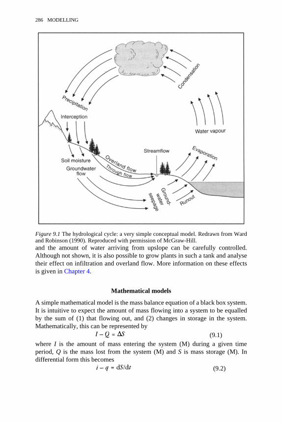
and the amount of water arriving from upslope can be carefully controlled.Although not shown, it is also possible to grow plants in such a tank and analysetheir effect on infiltration and overland flow. More information on these effectsis given in Chapter 4.
Mathematical models
A simple mathematical model is the mass balance equation of a black box system.It is intuitive to expect the amount of mass flowing into a system to be equalledby the sum of (1) that flowing out, and (2) changes in storage in the system.Mathematically, this can be represented by
(9.1)where I is the amount of mass entering the system (M) during a given timeperiod, Q is the mass lost from the system (M) and S is mass storage (M). Indifferential form this becomes
(9.2)
Figure 9.1 The hydrological cycle: a very simple conceptual model. Redrawn from Wardand Robinson (1990). Reproduced with permission of McGraw-Hill.
286 MODELLING
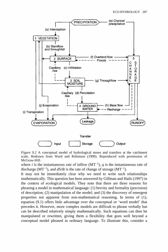
where i is the instantaneous rate of inflow (MT−1), q is the instantaneous rate ofdischarge (MT−1), and dS/dt is the rate of change of storage (MT−1). It may not be immediately clear why we need to write such relationshipsmathematically. This question has been answered by Gillman and Hails (1997) inthe context of ecological models. They note that there are three reasons forphrasing a model in mathematical language: (1) brevity and formality (precision)of description; (2) manipulation of the model; and (3) the discovery of emergentproperties not apparent from non-mathematical reasoning. In terms of (1),equation (9.1) offers little advantage over the conceptual or ‘word model’ thatprecedes it. However, more complex models are difficult to phrase verbally butcan be described relatively simply mathematically. Such equations can then bemanipulated or rewritten, giving them a flexibility that goes well beyond aconceptual model phrased in ordinary language. To illustrate this, consider a
Figure 9.2 A conceptual model of hydrological stores and transfers at the catchmentscale. Redrawn from Ward and Robinson (1990). Reproduced with permission ofMcGraw-Hill.
ECO-HYDROLOGY 287
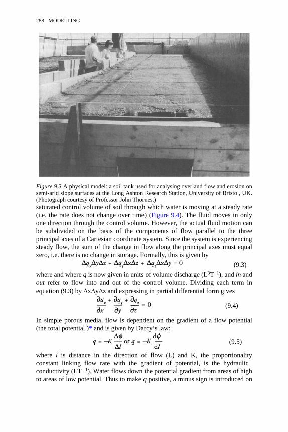
saturated control volume of soil through which water is moving at a steady rate(i.e. the rate does not change over time) (Figure 9.4). The fluid moves in onlyone direction through the control volume. However, the actual fluid motion canbe subdivided on the basis of the components of flow parallel to the threeprincipal axes of a Cartesian coordinate system. Since the system is experiencingsteady flow, the sum of the change in flow along the principal axes must equalzero, i.e. there is no change in storage. Formally, this is given by
(9.3)where and where q is now given in units of volume discharge (L3T−1), and in andout refer to flow into and out of the control volume. Dividing each term inequation (9.3) by ∆x∆y∆z and expressing in partial differential form gives
(9.4)
In simple porous media, flow is dependent on the gradient of a flow potential(the total potential )* and is given by Darcy’s law:
(9.5)
where l is distance in the direction of flow (L) and K, the proportionalityconstant linking flow rate with the gradient of potential, is the hydraulic conductivity (LT−1). Water flows down the potential gradient from areas of highto areas of low potential. Thus to make q positive, a minus sign is introduced on
Figure 9.3 A physical model: a soil tank used for analysing overland flow and erosion onsemi-arid slope surfaces at the Long Ashton Research Station, University of Bristol, UK.(Photograph courtesy of Professor John Thornes.)
288 MODELLING

the right-hand side of the equation. The flow potential is a measure of the energyavailable to do work in moving groundwater and consists of the sum of a numberof components, two of which are most important, i.e.
(9.6)where is the pressure or matric potential and is the elevation potential (Hillel,1980). Osmotic potentials are rarely important in soil- and groundwater flow.Expressed as a head, potential has dimensions of length. The three-dimensionalgeneralisation of Darcy’s law requires that the one-dimensional form be true foreach of the x, y and z components of flow. Assuming that the medium throughwhich water flows is isotropic (i.e. the hydraulic properties of the medium at apoint do not vary according to direction*) we can write
Substituting these into equation (9.4) gives
(9.7)
where . If K is assumed to be independent of x, y and z, i.e. the region is assumedto be homogeneous as well as isotropic, then equation (9.6) becomes
Figure 9.4 A saturated control volume for analysing flow through a soil.
* The convention in ground-water hydrology is to use to denote flow or total potential. Inkeeping with this convention, this notation is used here. Note, however, that it differs fromthat used by Tyree (see Chapter 2), where ψ is used to denote total potential (equation (2.5)).
ECO-HYDROLOGY 289
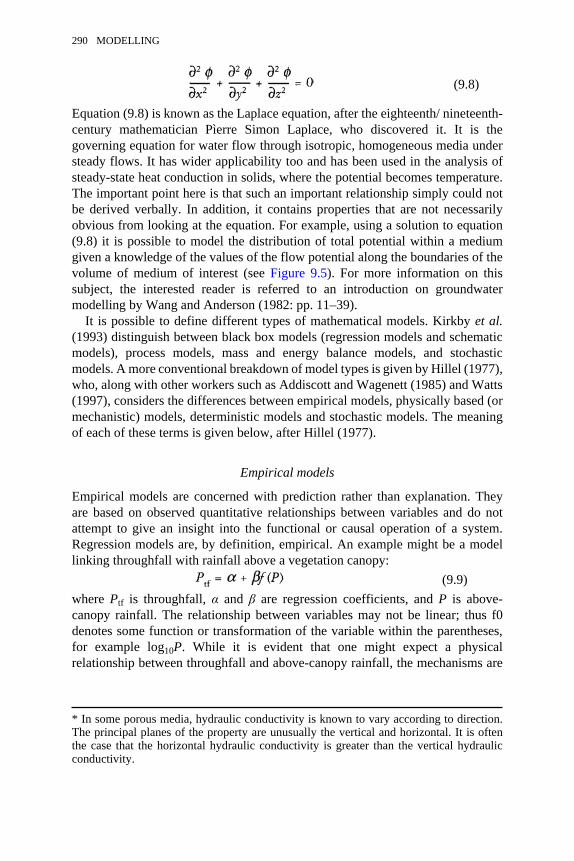
(9.8)
Equation (9.8) is known as the Laplace equation, after the eighteenth/ nineteenth-century mathematician Pìerre Simon Laplace, who discovered it. It is thegoverning equation for water flow through isotropic, homogeneous media understeady flows. It has wider applicability too and has been used in the analysis ofsteady-state heat conduction in solids, where the potential becomes temperature.The important point here is that such an important relationship simply could notbe derived verbally. In addition, it contains properties that are not necessarilyobvious from looking at the equation. For example, using a solution to equation(9.8) it is possible to model the distribution of total potential within a mediumgiven a knowledge of the values of the flow potential along the boundaries of thevolume of medium of interest (see Figure 9.5). For more information on thissubject, the interested reader is referred to an introduction on groundwatermodelling by Wang and Anderson (1982: pp. 11–39).
It is possible to define different types of mathematical models. Kirkby et al.(1993) distinguish between black box models (regression models and schematicmodels), process models, mass and energy balance models, and stochasticmodels. A more conventional breakdown of model types is given by Hillel (1977),who, along with other workers such as Addiscott and Wagenett (1985) and Watts(1997), considers the differences between empirical models, physically based (ormechanistic) models, deterministic models and stochastic models. The meaningof each of these terms is given below, after Hillel (1977).
Empirical models
Empirical models are concerned with prediction rather than explanation. Theyare based on observed quantitative relationships between variables and do notattempt to give an insight into the functional or causal operation of a system.Regression models are, by definition, empirical. An example might be a modellinking throughfall with rainfall above a vegetation canopy:
(9.9)where Ptf is throughfall, α and β are regression coefficients, and P is above-canopy rainfall. The relationship between variables may not be linear; thus f0denotes some function or transformation of the variable within the parentheses,for example log10P. While it is evident that one might expect a physicalrelationship between throughfall and above-canopy rainfall, the mechanisms are
* In some porous media, hydraulic conductivity is known to vary according to direction.The principal planes of the property are unusually the vertical and horizontal. It is oftenthe case that the horizontal hydraulic conductivity is greater than the vertical hydraulicconductivity.
290 MODELLING
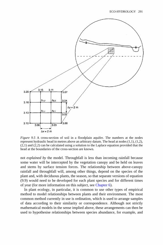
not explained by the model. Throughfall is less than incoming rainfall becausesome water will be intercepted by the vegetation canopy and be held on leavesand stems by surface tension forces. The relationship between above-canopyrainfall and throughfall will, among other things, depend on the species of theplant and, with deciduous plants, the season, so that separate versions of equation(9.9) would need to be developed for each plant species and for different timesof year (for more information on this subject, see Chapter 6).
In plant ecology, in particular, it is common to use other types of empiricalmethod to model relationships between plants and their environment. The mostcommon method currently in use is ordination, which is used to arrange samplesof data according to their similarity or correspondence. Although not strictlymathematical models in the sense implied above, these arrangements can then beused to hypothesise relationships between species abundance, for example, and
Figure 9.5 A cross-section of soil in a floodplain aquifer. The numbers at the nodesrepresent hydraulic head in metres above an arbitrary datum. The head at nodes (1,1), (1,2),(2,1) and (2,2) can be calculated using a solution to the Laplace equation provided that thehead at the boundaries of the cross-section are known.
ECO-HYDROLOGY 291
various environmental factors such as degree of wetness (waterlogging). Detailsof the method can be found in Goldsmith et al. (1986). One of the mostcommonly used ordination methods is detrended correspondence analysis (DCA)(the computer program is called DECORANA; Hill, 1979). A good example ofthe use of DCA is Busch et al. (1998), who looked at the relationship betweenplant communities and hydrological variables in the Florida Everglades, USA.
Physically based or mechanistic models
Physically based models are based on known mechanisms or processes thatoperate within the system being modelled. These mechanisms are described bythe fundamental laws of physics and chemistry. It is important to note that‘physically based’ does not necessarily mean that the model is entirely composedof fundamental physical laws, merely that it is based to a large extent on suchlaws. Models that combine significant elements of both the physical andempirical approaches are often called semi-empirical. A good example of aphysically based model is the Penman-Monteith equation (Penman, 1948;Monteith, 1973—see Campbell, 1981) used to predict evapotranspiration from avegetated surface (see also Chapter 2). Physically based models have also beencalled theoretical models because they are essentially statements of how wethink the real world behaves as opposed to an empirical model, which describesthe behaviour of one variable in terms of another without any attempt to explainsystem behaviour. Theoretical models are widely used in research and representformal statements of theories, which should then be tested with experimentaldata.
Deterministic models
With deterministic models exact relationships are postulated, and the output ofthe model is predicted with complete certainty by the input. Thus the watercontent of a length of river channel can be calculated with certainty for all timeswhen the initial storage, as well as the inflows and outflows from the channel, isknown. Deterministic models can be both empirical and physically based. Inequation (9.9), the amount of throughfall is given exactly from a knowledge ofabove-canopy rainfall. This does not mean to say that the prediction of the modelis correct, merely that for a given input, the model will produce a unique output.
Stochastic models
In stochastic models, a random or stochastic element is introduced into themodel so that for a given input there is no longer a single output but a range ordistribution of output values. For example, equation (9.9) could be rewritten
(9.10)
292 MODELLING
where r is a random value or variable that has different values for each run of themodel, even if the values of the model inputs remain the same. Thus, Ptf is nolonger a unique function of P but also depends on r, which is randomly generatedfor each model run. r will usually be generated from a known probabilitydistribution (Kirkby et al., 1993). Sometimes, the term stochastic model is alsoused to describe Monte Carlo simulations using deterministic models. MonteCarlo simulations are used where there is some uncertainty in the input data. Thusinput data sets are drawn from measured or assumed distributions of inputparameters. The probability of different model outputs can then be determined byanalysing the distribution of model outputs. For an example of a Monte Carlosimulation using an eco-hydrological model, see Franks and Beven (1997).
Other model types
Continuous models portray continuous processes, in contrast to discrete modelswhich include discontinuous or abrupt phenomena. Dynamic models simulatetime-dependent processes, as opposed to static systems or systems in whichprocesses operate at a steady rate (steady-state models are then used). Twoclasses of model not explicitly discussed by Hillel (1977) are lumped anddistributed models. In lumped models, no attempt is made to account for spatialvariability of a given process. Many conceptual mathematical models are of thelumped type in which the river catchment is represented as a series of conceptualstores, with stores representing the soil system, the channel system and so on.Such a model, HYRROM (HYdrological Rainfall Runoff Model) (Blackie andEeles, 1985), is illustrated in Figure 9.6, where it can be seen that the catchmentis conceptualised as four lumped stores: the vegetation canopy, the soil, thegroundwater store, and the channel or routing store. Flow from the soil,groundwater and routing stores is described mathematically as a function of thewater content of each store. The flow equations used in the model are notexplained here, and the interested reader should refer to the original paper.Distributed models explicitly account for spatial variations in parameter valuesand rates of process operation. Most account for such variation by ‘chopping up’the system of interest, such as a river catchment or hill slope, into a series ofstores. Thus for a catchment there may be hundreds or even thousands of soilstores, each representing different soil types or variations within a soil type,thousands of stores representing the river channel network and so on. This isillustrated below (see Figure 9.7).
WHAT IS AN ECO-HYDROLOGICAL MODEL?
In its broadest sense, an eco-hydrological model is any model used in anecohydrological study. Thus, for example, Wassen et al. (1996) use agroundwater flow model (FLOWNET—van Elburg et al., 1991) to indicatepossible pathways of water movement into and out of fens in order to understand
ECO-HYDROLOGY 293
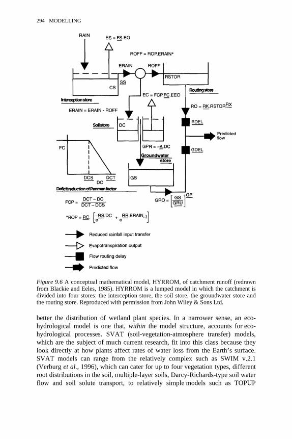
better the distribution of wetland plant species. In a narrower sense, an eco-hydrological model is one that, within the model structure, accounts for eco-hydrological processes. SVAT (soil-vegetation-atmosphere transfer) models,which are the subject of much current research, fit into this class because theylook directly at how plants affect rates of water loss from the Earth’s surface.SVAT models can range from the relatively complex such as SWIM v.2.1(Verburg et al., 1996), which can cater for up to four vegetation types, differentroot distributions in the soil, multiple-layer soils, Darcy-Richards-type soil waterflow and soil solute transport, to relatively simple models such as TOPUP
Figure 9.6 A conceptual mathematical model, HYRROM, of catchment runoff (redrawnfrom Blackie and Eeles, 1985). HYRROM is a lumped model in which the catchment isdivided into four stores: the interception store, the soil store, the groundwater store andthe routing store. Reproduced with permission from John Wiley & Sons Ltd.
294 MODELLING

(Quinn et al., 1995; see also McGuffie and Henderson-Sellers, 1997). Other eco-hydrological models that deal with SVAT and plant growth, such as thePATTERN model, have also been discussed in this volume (see Chapter 4).However, even in these ‘true’ ecohydrological models there are hydrological sub-models. Thus the distinction made above between the broad and narrowdefinitions is rather artificial. In this chapter, the broader definition is used, sincemany more examples of hydrological models exist than true eco-hydrologicalmodels, and because many of the points in the chapter deal with modelling issuesin general that can be adequately illustrated with hydrological models.
SIMPLICITY AND COMPLEXITY OF MODELS
The main part of this chapter begins with the question of simplicity andcomplexity: in other words, how detailed should we make our models? This isnot a trivial question and might at first seem a very difficult one to answer, asthis quote from Eagleton (1986: p. 149) suggests: ‘For if the complex can be putinto the simple, then it was not as complex as it seemed in the first place; and ifthe simple can be an adequate medium of such complexity, then it cannot afterall be as simple as all that.’
If we were to accept the cynicism of Eagleton, then we might not make anyprogress in modelling complex systems. Fortunately, the question has also beensummed up, more prosaically but more usefully, by Gleick (1988):
The choice is always the same. You can make your model more complexand more faithful to reality, or you can make it simpler and easier tohandle. Only the most naive scientist believes that the perfect model is theone that perfectly represents reality. Such a model would have the samedrawbacks as a map as large and detailed as the city it represents, a mapdepicting every park, every street, every building, every tree, everypothole, every inhabitant, and every map. Were such a map possible, itsspecificity would defeat its purpose: to generalise and abstract.
Gleick’s message is clear: models should always attempt to simplify and weshould be wary of complexity in model design, because with a complex modelwe can lose the power of abstraction. In any case, as workers on deterministicchaos have demonstrated, even simple models can display complex behaviourand we should, perhaps, try to understand these simple models before we attemptto build more complex ones.
If the purpose of a model is, as Gleick suggests, to generalise and abstract, it isperhaps surprising to see so many complex models in the academic andprofessional literature. Put harshly, it is almost as if we are scared toleave something out of our models in case we miss some important aspect ofsystem behaviour. There is also the possibility of ‘model snobbery’: ‘My modelis bigger than yours and has more “governing” equations; therefore, it must be a
ECO-HYDROLOGY 295
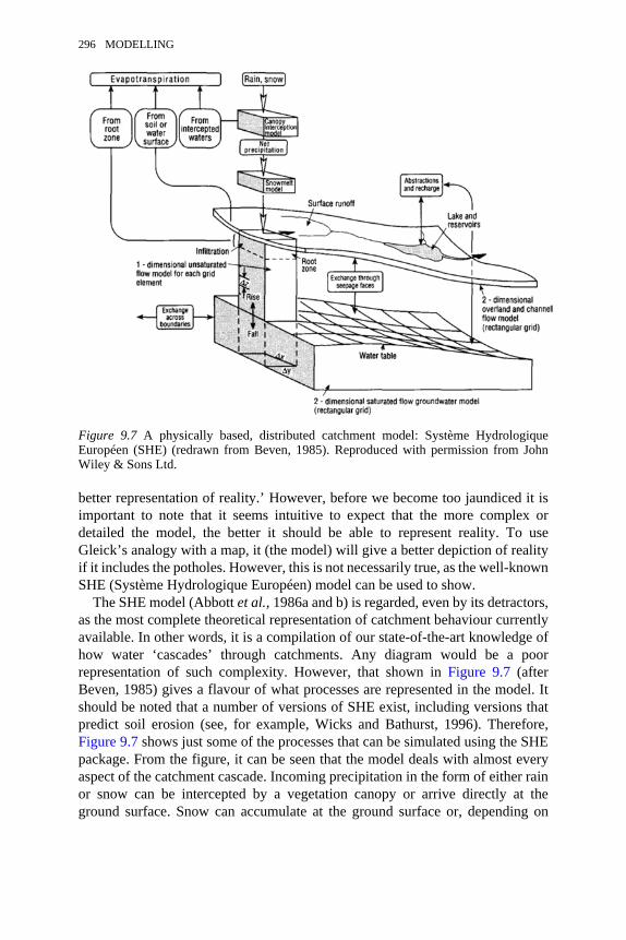
better representation of reality.’ However, before we become too jaundiced it isimportant to note that it seems intuitive to expect that the more complex ordetailed the model, the better it should be able to represent reality. To useGleick’s analogy with a map, it (the model) will give a better depiction of realityif it includes the potholes. However, this is not necessarily true, as the well-knownSHE (Système Hydrologique Européen) model can be used to show.
The SHE model (Abbott et al., 1986a and b) is regarded, even by its detractors,as the most complete theoretical representation of catchment behaviour currentlyavailable. In other words, it is a compilation of our state-of-the-art knowledge ofhow water ‘cascades’ through catchments. Any diagram would be a poorrepresentation of such complexity. However, that shown in Figure 9.7 (afterBeven, 1985) gives a flavour of what processes are represented in the model. Itshould be noted that a number of versions of SHE exist, including versions thatpredict soil erosion (see, for example, Wicks and Bathurst, 1996). Therefore,Figure 9.7 shows just some of the processes that can be simulated using the SHEpackage. From the figure, it can be seen that the model deals with almost everyaspect of the catchment cascade. Incoming precipitation in the form of either rainor snow can be intercepted by a vegetation canopy or arrive directly at theground surface. Snow can accumulate at the ground surface or, depending on
Figure 9.7 A physically based, distributed catchment model: Système HydrologiqueEuropéen (SHE) (redrawn from Beven, 1985). Reproduced with permission from JohnWiley & Sons Ltd.
296 MODELLING
meteorological variables, can melt. Water is lost directly from the catchmentthrough the processes of evapotranspiration. Water accumulating at the soilsurface can infiltrate into the soil and move through the unsaturated zone either asthroughflow or vertically into the deeper groundwater zone. If infiltration isinsufficient to prevent ponding of water at the soil surface, or if the water tablerises to the surface to cause ponding, overland flow or surface runoff will occur.This water will eventually enter the channel network and flow to the catchmentoutlet. Deeper groundwater flow is also simulated. A concise review of theseprocesses is given by Baird (1997a), while a good detailed treatment is given byDingman (1994). The SHE model is also a distributed model, as can be seenclearly from Figure 9.7. The catchment is divided into a grid, and for every grid‘cell’, each of the processes listed above is, where relevant, simulated. Thus for agiven cell the following processes could be simulated: canopy interception,evapotranspiration, soil water flow, groundwater flow and surface runoff. In asense, each grid cell is like a mini lumped model. By having a large number ofthese cells, SHE is able to simulate spatial variations in processes across thecatchment. The model is a statement of classic reductionist thinking in eco-hydrology: to understand catchment behaviour it is best to divide up thecatchment into its component physical and process parts.
Has SHE been successful? Some would argue that it has. They would suggestthat as a theoretical tool it can give an insight into how a fictitious catchmentmight be expected to ‘behave’ given a particular set of (input) conditions. It canbe used to answer (theoretical) questions on, for example, what happens tostreamflow if a woodland is removed in one part of the modelled catchment. In amore practical sense the model has also been used to predict successfullystreamflow data from real-world catchments (Bathurst, 1986; Bathurst et al.,1996). However, this is where we can identify weaknesses in the model. It ispossible for a complex model to give the right results for the wrong reasons. Ifthe model is sufficiently complex, and knowledge of parameter valuessufficiently uncertain, then it is possible to get the right answer (stream dischargefrom a catchment) by representing the wrong processes within the modelledsystem. For example, consider a situation in which rapid catchment (streamflow)response to rainfall has been observed. This could occur for a variety of reasonsand will probably depend on the hydraulic properties of the soil. However, ourknowledge of the range of soil hydraulic conductivities in the real catchment islikely to be scanty at best. Such data are time-consuming and expensive tocollect. As an alternative to collecting data on hydraulic conductivity from everypart of a catchment and for every layer of soil, researchers will estimate values ofthe parameter. Estimation is, by definition, an uncertain procedure, so ranges ofpossible values for the parameter will be used. The values of many parameters ina model such as SHE will be estimated. The range of uncertainty for eachparameter is often sufficiently large that it is possible for a model such as SHE tobe run with quite different sets of apparently realistic input conditions and givethe same or very similar results in terms of water discharging from the
ECO-HYDROLOGY 297
catchment. For example, a rapid streamflow response could be predicted whenhigh-permeability subsoils allow rapid throughflow to the channel in the modelcatchment. A very similar discharge time series could be predicted when themodel catchment contains low-permeability subsoils in the vicinity of streamchannels. During rainfall, these will prevent downward percolation of waterthrough the soil profile, causing a rapid rise in the (perched) water table. If thewater table intercepts the soil surface, overland flow may occur, causingrainwater to flow rapidly to the channel system. We therefore have a situationwhere quite different processes (overland flow and rapid throughflow) occurringwithin the model catchment give very similar outcomes in terms of streamflowresponse to rainfall. This is equifinality, or more strictly model equifinality, asdefined by Beven (1996) and discussed in the context of other hydrological andeco-hydrological models models by Grayson et al. (1992) and Franks et al.(1997). The important point here is that, as modellers, we have been unable toidentify what is going on in the real world: we do not know whether overlandflow or rapid throughflow is the reason for the observed rapid streamflowresponse to rainfall. Both are plausible given our uncertain knowledge aboutinput conditions. This is the problem of model and parameter identifiability orindeterminancy (Kennedy, 1985). We have developed a model that purports torepresent the real world to a high level of physical detail. In practice, we havedeveloped a very expensive computer code that, although it can be used to obtainaccurate predictions of streamflow, cannot necessarily be used to give insightsinto what is going on physically in the real catchment. The model has, therefore,failed to do what it was set up for. It is likely that we could achieve similar levelsof predictive accuracy using a much simpler conceptual mathematical store andflow model with just a few parameters. To find out why the real catchmentshows the response it does would require detailed field observations to determinewhether or not overland flow and rapid throughflow occur. It is important torealise that just because a physically based model accurately predicts some aspectof real system behaviour does not guarantee that it has done so by representingthe real system accurately.
The famous mathematician and physicist Roger Penrose has classified theoriesas ‘superb’, ‘useful’, ‘tentative’ and ‘misguided’ (Gardner, 1989). Such a four-fold classification could also be applied to models. Some would argue that SHEand like models are superb; others, myself included, would suggest that they aretentative.
A BLUEPRINT FOR BETTER MODELLING?
If models such as SHE are tentative, how can we set about producing bettermodels? Is it possible to set up a blueprint for better modelling? The answer to thisis probably a qualified ‘yes’, although, as will be shown below, modelconstruction and testing are more difficult than they first appear. Among others,Kirkby et al. (1993) have suggested that choice of an appropriate model should
298 MODELLING
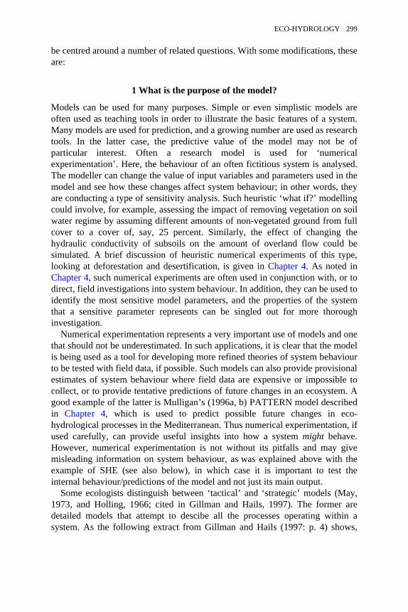
be centred around a number of related questions. With some modifications, theseare:
1 What is the purpose of the model?
Models can be used for many purposes. Simple or even simplistic models areoften used as teaching tools in order to illustrate the basic features of a system.Many models are used for prediction, and a growing number are used as researchtools. In the latter case, the predictive value of the model may not be ofparticular interest. Often a research model is used for ‘numericalexperimentation’. Here, the behaviour of an often fictitious system is analysed.The modeller can change the value of input variables and parameters used in themodel and see how these changes affect system behaviour; in other words, theyare conducting a type of sensitivity analysis. Such heuristic ‘what if?’ modellingcould involve, for example, assessing the impact of removing vegetation on soilwater regime by assuming different amounts of non-vegetated ground from fullcover to a cover of, say, 25 percent. Similarly, the effect of changing thehydraulic conductivity of subsoils on the amount of overland flow could besimulated. A brief discussion of heuristic numerical experiments of this type,looking at deforestation and desertification, is given in Chapter 4. As noted inChapter 4, such numerical experiments are often used in conjunction with, or todirect, field investigations into system behaviour. In addition, they can be used toidentify the most sensitive model parameters, and the properties of the systemthat a sensitive parameter represents can be singled out for more thoroughinvestigation.
Numerical experimentation represents a very important use of models and onethat should not be underestimated. In such applications, it is clear that the modelis being used as a tool for developing more refined theories of system behaviourto be tested with field data, if possible. Such models can also provide provisionalestimates of system behaviour where field data are expensive or impossible tocollect, or to provide tentative predictions of future changes in an ecosystem. Agood example of the latter is Mulligan’s (1996a, b) PATTERN model describedin Chapter 4, which is used to predict possible future changes in eco-hydrological processes in the Mediterranean. Thus numerical experimentation, ifused carefully, can provide useful insights into how a system might behave.However, numerical experimentation is not without its pitfalls and may givemisleading information on system behaviour, as was explained above with theexample of SHE (see also below), in which case it is important to test theinternal behaviour/predictions of the model and not just its main output.
Some ecologists distinguish between ‘tactical’ and ‘strategic’ models (May,1973, and Holling, 1966; cited in Gillman and Hails, 1997). The former aredetailed models that attempt to descibe all the processes operating within asystem. As the following extract from Gillman and Hails (1997: p. 4) shows,
ECO-HYDROLOGY 299
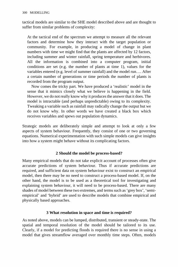
tactical models are similar to the SHE model described above and are thought tosuffer from similar problems of complexity:
At the tactical end of the spectrum we attempt to measure all the relevantfactors and determine how they interact with the target population orcommunity. For example, in producing a model of change in plantnumbers with time we might find that the plants are affected by 12 factors,including summer and winter rainfall, spring temperature and herbivores.All the information is combined into a computer program, initialconditions are set (e.g. the number of plants at time 1), values for thevariables entered (e.g. level of summer rainfall) and the model run…. Aftera certain number of generations or time periods the number of plants isrecorded from the program output.
Now comes the tricky part. We have produced a ‘realistic’ model in thesense that it mimics closely what we believe is happening in the field.However, we do not really know why it produces the answer that it does. Themodel is intractable (and perhaps unpredictable) owing to its complexity.Tweaking a variable such as rainfall may radically change the output but wedo not know why. In other words we have created a black box whichreceives variables and spews out population dynamics.
Strategic models are deliberately simple and attempt to look at only a fewaspects of system behaviour. Frequently, they consist of one or two governingequations. Numerical experimentation with such simple models can give insightsinto how a system might behave without its complicating factors.
2 Should the model be process-based?
Many empirical models that do not take explicit account of processes often giveaccurate predictions of system behaviour. Thus if accurate predictions arerequired, and sufficient data on system behaviour exist to construct an empiricalmodel, then there may be no need to construct a process-based model. If, on theother hand, the model is to be used as a theoretical tool for investigating andexplaining system behaviour, it will need to be process-based. There are manyshades of model between these two extremes, and terms such as ‘grey box’, ‘semi-empirical’ and ‘hybrid’ are used to describe models that combine empirical andphysically based approaches.
3 What resolution in space and time is required?
As noted above, models can be lumped, distributed, transient or steady-state. Thespatial and temporal resolution of the model should be tailored to its use.Clearly, if a model for predicting floods is required there is no sense in using amodel that gives streamflow averaged over monthly time steps. Often, models
300 MODELLING
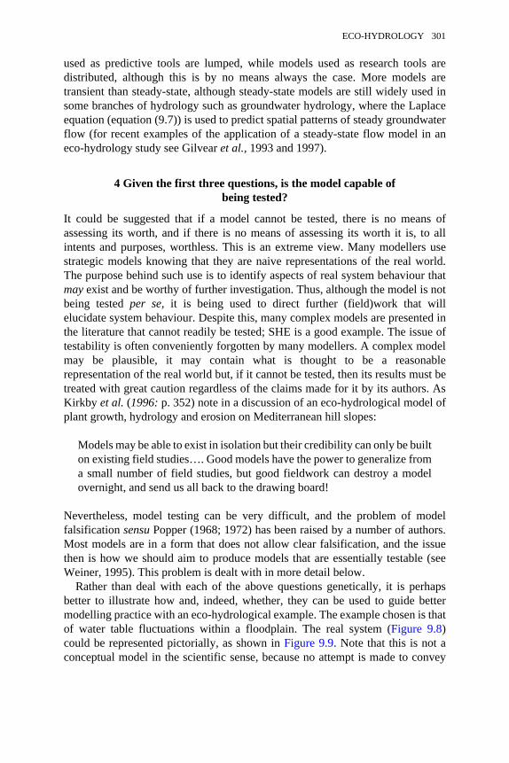
used as predictive tools are lumped, while models used as research tools aredistributed, although this is by no means always the case. More models aretransient than steady-state, although steady-state models are still widely used insome branches of hydrology such as groundwater hydrology, where the Laplaceequation (equation (9.7)) is used to predict spatial patterns of steady groundwaterflow (for recent examples of the application of a steady-state flow model in aneco-hydrology study see Gilvear et al., 1993 and 1997).
4 Given the first three questions, is the model capable ofbeing tested?
It could be suggested that if a model cannot be tested, there is no means ofassessing its worth, and if there is no means of assessing its worth it is, to allintents and purposes, worthless. This is an extreme view. Many modellers usestrategic models knowing that they are naive representations of the real world.The purpose behind such use is to identify aspects of real system behaviour thatmay exist and be worthy of further investigation. Thus, although the model is notbeing tested per se, it is being used to direct further (field)work that willelucidate system behaviour. Despite this, many complex models are presented inthe literature that cannot readily be tested; SHE is a good example. The issue oftestability is often conveniently forgotten by many modellers. A complex modelmay be plausible, it may contain what is thought to be a reasonablerepresentation of the real world but, if it cannot be tested, then its results must betreated with great caution regardless of the claims made for it by its authors. AsKirkby et al. (1996: p. 352) note in a discussion of an eco-hydrological model ofplant growth, hydrology and erosion on Mediterranean hill slopes:
Models may be able to exist in isolation but their credibility can only be builton existing field studies…. Good models have the power to generalize froma small number of field studies, but good fieldwork can destroy a modelovernight, and send us all back to the drawing board!
Nevertheless, model testing can be very difficult, and the problem of modelfalsification sensu Popper (1968; 1972) has been raised by a number of authors.Most models are in a form that does not allow clear falsification, and the issuethen is how we should aim to produce models that are essentially testable (seeWeiner, 1995). This problem is dealt with in more detail below.
Rather than deal with each of the above questions genetically, it is perhapsbetter to illustrate how and, indeed, whether, they can be used to guide bettermodelling practice with an eco-hydrological example. The example chosen is thatof water table fluctuations within a floodplain. The real system (Figure 9.8)could be represented pictorially, as shown in Figure 9.9. Note that this is not aconceptual model in the scientific sense, because no attempt is made to convey
ECO-HYDROLOGY 301
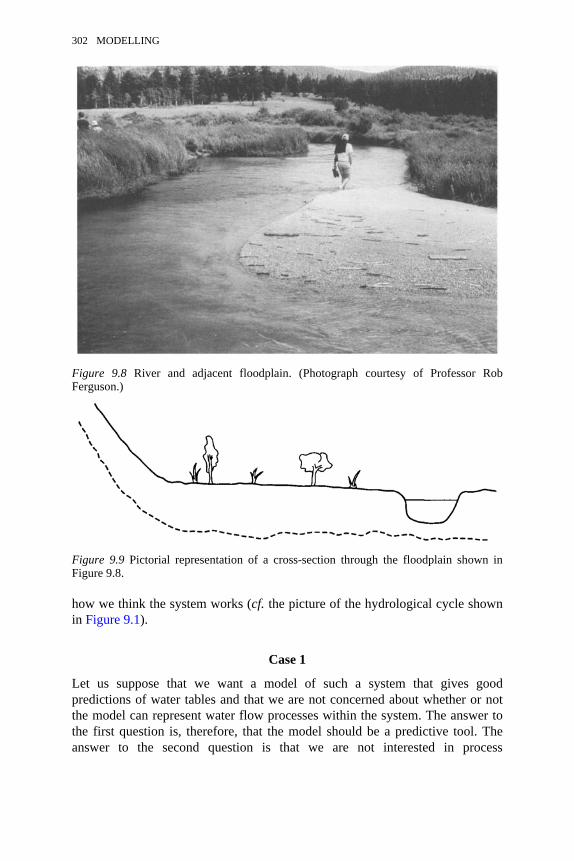
how we think the system works (cf. the picture of the hydrological cycle shownin Figure 9.1).
Case 1
Let us suppose that we want a model of such a system that gives goodpredictions of water tables and that we are not concerned about whether or notthe model can represent water flow processes within the system. The answer tothe first question is, therefore, that the model should be a predictive tool. Theanswer to the second question is that we are not interested in process
Figure 9.8 River and adjacent floodplain. (Photograph courtesy of Professor RobFerguson.)
Figure 9.9 Pictorial representation of a cross-section through the floodplain shown inFigure 9.8.
302 MODELLING
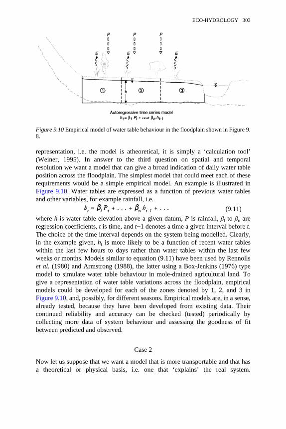
representation, i.e. the model is atheoretical, it is simply a ‘calculation tool’(Weiner, 1995). In answer to the third question on spatial and temporalresolution we want a model that can give a broad indication of daily water tableposition across the floodplain. The simplest model that could meet each of theserequirements would be a simple empirical model. An example is illustrated inFigure 9.10. Water tables are expressed as a function of previous water tablesand other variables, for example rainfall, i.e.
(9.11)where h is water table elevation above a given datum, P is rainfall, βl to βn areregression coefficients, t is time, and t−1 denotes a time a given interval before t.The choice of the time interval depends on the system being modelled. Clearly,in the example given, ht is more likely to be a function of recent water tableswithin the last few hours to days rather than water tables within the last fewweeks or months. Models similar to equation (9.11) have been used by Rennollset al. (1980) and Armstrong (1988), the latter using a Box-Jenkins (1976) typemodel to simulate water table behaviour in mole-drained agricultural land. Togive a representation of water table variations across the floodplain, empiricalmodels could be developed for each of the zones denoted by 1, 2, and 3 inFigure 9.10, and, possibly, for different seasons. Empirical models are, in a sense,already tested, because they have been developed from existing data. Theircontinued reliability and accuracy can be checked (tested) periodically bycollecting more data of system behaviour and assessing the goodness of fitbetween predicted and observed.
Case 2
Now let us suppose that we want a model that is more transportable and that hasa theoretical or physical basis, i.e. one that ‘explains’ the real system.
Figure 9.10 Empirical model of water table behaviour in the floodplain shown in Figure 9.8.
ECO-HYDROLOGY 303
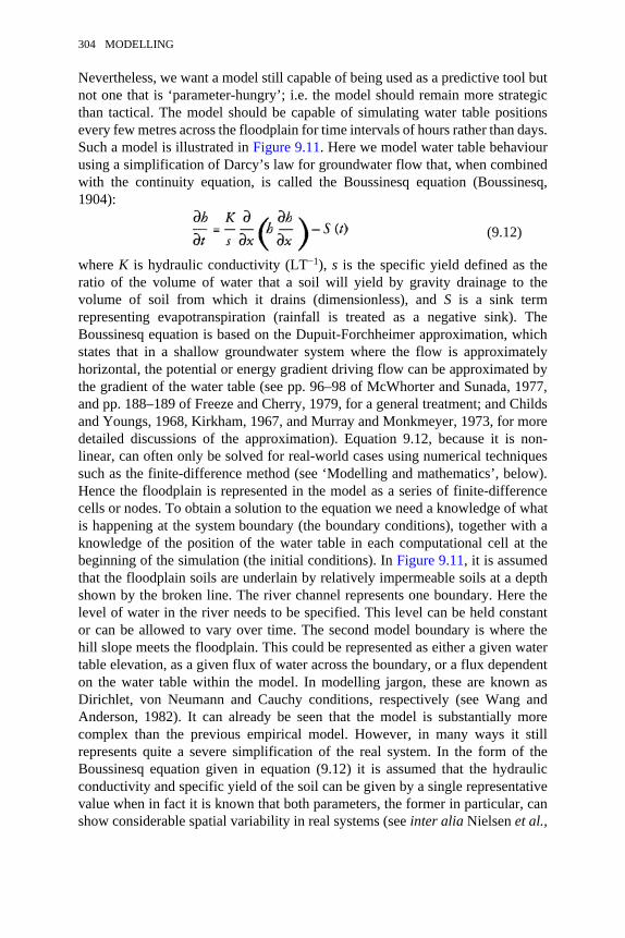
Nevertheless, we want a model still capable of being used as a predictive tool butnot one that is ‘parameter-hungry’; i.e. the model should remain more strategicthan tactical. The model should be capable of simulating water table positionsevery few metres across the floodplain for time intervals of hours rather than days.Such a model is illustrated in Figure 9.11. Here we model water table behaviourusing a simplification of Darcy’s law for groundwater flow that, when combinedwith the continuity equation, is called the Boussinesq equation (Boussinesq,1904):
(9.12)
where K is hydraulic conductivity (LT−1), s is the specific yield defined as theratio of the volume of water that a soil will yield by gravity drainage to thevolume of soil from which it drains (dimensionless), and S is a sink termrepresenting evapotranspiration (rainfall is treated as a negative sink). TheBoussinesq equation is based on the Dupuit-Forchheimer approximation, whichstates that in a shallow groundwater system where the flow is approximatelyhorizontal, the potential or energy gradient driving flow can be approximated bythe gradient of the water table (see pp. 96–98 of McWhorter and Sunada, 1977,and pp. 188–189 of Freeze and Cherry, 1979, for a general treatment; and Childsand Youngs, 1968, Kirkham, 1967, and Murray and Monkmeyer, 1973, for moredetailed discussions of the approximation). Equation 9.12, because it is non-linear, can often only be solved for real-world cases using numerical techniquessuch as the finite-difference method (see ‘Modelling and mathematics’, below).Hence the floodplain is represented in the model as a series of finite-differencecells or nodes. To obtain a solution to the equation we need a knowledge of whatis happening at the system boundary (the boundary conditions), together with aknowledge of the position of the water table in each computational cell at thebeginning of the simulation (the initial conditions). In Figure 9.11, it is assumedthat the floodplain soils are underlain by relatively impermeable soils at a depthshown by the broken line. The river channel represents one boundary. Here thelevel of water in the river needs to be specified. This level can be held constantor can be allowed to vary over time. The second model boundary is where thehill slope meets the floodplain. This could be represented as either a given watertable elevation, as a given flux of water across the boundary, or a flux dependenton the water table within the model. In modelling jargon, these are known asDirichlet, von Neumann and Cauchy conditions, respectively (see Wang andAnderson, 1982). It can already be seen that the model is substantially morecomplex than the previous empirical model. However, in many ways it stillrepresents quite a severe simplification of the real system. In the form of theBoussinesq equation given in equation (9.12) it is assumed that the hydraulicconductivity and specific yield of the soil can be given by a single representativevalue when in fact it is known that both parameters, the former in particular, canshow considerable spatial variability in real systems (see inter alia Nielsen et al.,
304 MODELLING
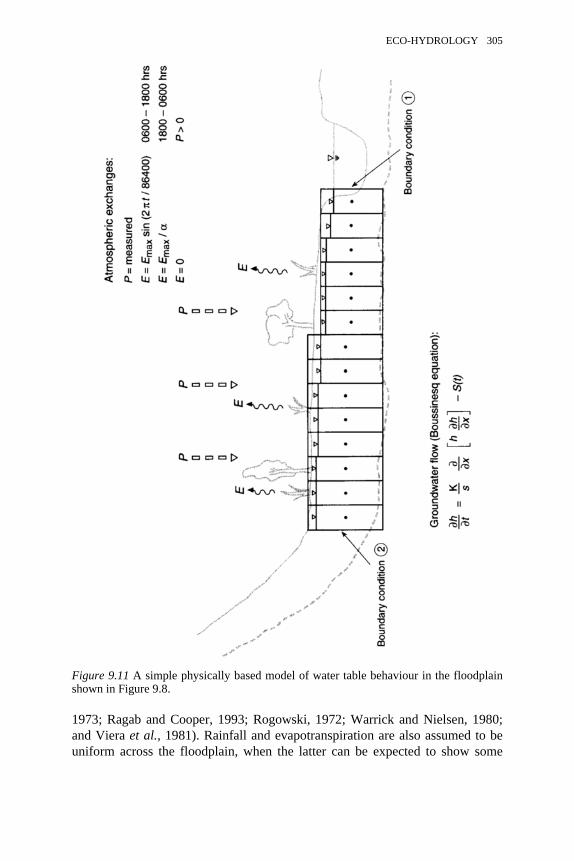
1973; Ragab and Cooper, 1993; Rogowski, 1972; Warrick and Nielsen, 1980;and Viera et al., 1981). Rainfall and evapotranspiration are also assumed to beuniform across the floodplain, when the latter can be expected to show some
Figure 9.11 A simple physically based model of water table behaviour in the floodplainshown in Figure 9.8.
ECO-HYDROLOGY 305
variability depending on the distribution of different vegetation types and watertable depths. In addition, no attempt is made to account for the effects of theunsaturated zone on water table behaviour. Thus rainfall is added directly to thewater table and is not taken up by storage in the unsaturated zone. This isprobably a reasonable assumption during winter, when the water table is close tothe ground surface, but it could be a source of error in model predictions duringlow water table conditions in summer months. Evapotranspiration is predictedusing a simple sine-wave model in which losses of water to the atmosphere varyas a function of the maximum (midday) measured evapotranspiration (see Hillelet al., 1976):
(9.13)
where E is evapotranspiration rate (m s−1), Emax is maximum middayevapotranspiration rate (m s−1), t is time (s), and α is an empirically determinedparameter (dimensionless). Obviously, such a model is very simple and does nottake explicit account of changes in atmospheric controls on the process. Innature, evapotranspiration rates are controlled principally by (1) the provision atthe evaporating surface of sufficient energy for the latent heat of vaporisationand the operation above the surface of diffusion and mixing processes, whichremove water vapour produced by evaporation, and (2) by the properties of thefloodplain vegetation (since these will affect wind flow in the boundary layer)and the depth of the water table (Gardner, 1957). Plants will also exert a controlon evapotranspiration through their stomatal resistance to vapour flux. For moreinformation on these processes, see Chapters 2 and 6.
How could such a model be tested? If one purpose of the model is to predict orrepresent water table behaviour across the floodplain, there is obviously a need tomeasure water tables at strategic locations away from the river. Lined augerholes could be used for such a purpose. Water will flow into or out of these inorder to attain equilibrium with the free water surface in the soil. If the time toattain equilibrium is relatively short, the auger holes should provide a goodmeasure of actual water table fluctuations. Having measured water tables, it isthen necessary to measure or estimate K and s and Emax. Once this has beendone, the predicted water tables could be compared with measured values toascertain the goodness of fit between the two. However, it is possible, even in thesimple model presented, that errors in the evapo-transporation sub-model couldcancel out errors in the groundwater flow model, giving a good fit betweenobserved and predicted water tables. Equally, a poor fit between observed andpredicted water tables could be due to only one, and not both, of the sub-models.In order to resolve this problem, the sub-models should be tested separately (thisis known as internal validation). For example, the groundwater model could be
306 MODELLING
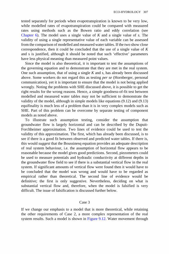
tested separately for periods when evapotranspiration is known to be very low,while modelled rates of evapotranspiration could be compared with measuredrates using methods such as the Bowen ratio and eddy correlation (seeChapter 6). The model uses a single value of K and a single value of s. Thevalidity of using a single representative value of each variable can be assessedfrom the comparison of modelled and measured water tables. If the two show closecorrespondence, then it could be concluded that the use of a single value of Kand s is justified, although it should be noted that such ‘effective’ parametershave less physical meaning than measured point values.
Since the model is also theoretical, it is important to test the assumptions ofthe governing equation and to demonstrate that they are met in the real system.One such assumption, that of using a single K and s, has already been discussedabove. Some workers do not regard this as testing per se (Hornberger, personalcommunication), yet it is important to ensure that the model is not being appliedwrongly. Noting the problems with SHE discussed above, it is possible to get theright results for the wrong reasons. Hence, a simple goodness-of-fit test betweenmodelled and measured water tables may not be sufficient to demonstrate thevalidity of the model, although in simple models like equations (9.12) and (9.13)equifinality is much less of a problem than it is in very complex models such asSHE. Part of this problem can be overcome by separate testing of componentmodels as noted above.
To illustrate such assumption testing, consider the assumption thatgroundwater flow is largely horizontal and can be described by the Dupuit-Forchheimer approximation. Two lines of evidence could be used to test thevalidity of this approximation. The first, which has already been discussed, is tosee if there is a good fit between observed and predicted water tables. If there is,this would suggest that the Boussinesq equation provides an adequate descriptionof real system behaviour, i.e. the assumption of horizontal flow appears to bereasonable because the model gives good predictions. Second, piezometers couldbe used to measure potentials and hydraulic conductivity at different depths inthe groundwater flow field to see if there is a substantial vertical flow in the realsystem. If significant amounts of vertical flow were found then it would have tobe concluded that the model was wrong and would have to be regarded asempirical rather than theoretical. The second line of evidence would bedefinitive; the first is only suggestive. Nevertheless, deciding on what issubstantial vertical flow and, therefore, when the model is falsified is verydifficult. The issue of falsification is discussed further below.
Case 3
If we change our emphasis to a model that is more theoretical, while retainingthe other requirements of Case 2, a more complex representation of the realsystem results. Such a model is shown in Figure 9.12. Water movement through
ECO-HYDROLOGY 307
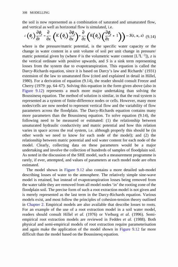
the soil is now represented as a combination of saturated and unsaturated flow,and vertical as well as horizontal flow is simulated, i.e.
(9.14)
where is the pressure/matric potential, is the specific water capacity or thechange in water content in a unit volume of soil per unit change in pressure/matric potential given by (where θ is the volumetric water content [L3L−3]), z isthe vertical ordinate with positive upwards, and S is a sink term representinglosses from the system due to evapotranspiration. This equation is called theDarcy-Richards equation, since it is based on Darcy’s law and Richards’ (1931)extension of the law to unsaturated flow (cited and explained in detail in Hillel,1980). For a derivation of equation (9.14), the reader should consult Freeze andCherry (1979: pp. 64–67). Solving this equation in the form given above (also inFigure 9.12) represents a much more major undertaking than solving theBoussinesq equation. The method of solution is similar, in that the real system isrepresented as a system of finite-difference nodes or cells. However, many morenodes/cells are now needed to represent vertical flow and the variability of flowparameters across the floodplain. The Darcy-Richards equation contains manymore parameters than the Boussinesq equation. To solve equation (9.14), thefollowing need to be measured or estimated: (1) the relationship betweenunsaturated hydraulic conductivity and matric potential and how this relationvaries in space across the real system, i.e. although properly this should be (inother words we need to know for each node of the model); and (2) therelationship between matric potential and soil water content for each node of themodel. Clearly, collecting data on these parameters would be a majorundertaking and involve the collection of hundreds of samples of floodplain soil.As noted in the discussion of the SHE model, such a measurement programme israrely, if ever, attempted, and values of parameters at each model node are oftenestimated.
The model shown in Figure 9.12 also contains a more detailed sub-modeldescribing losses of water to the atmosphere. The relatively simple sine-wavemodel is retained, but instead of evapotranspiration losses being removed fromthe water table they are removed from all model nodes ‘in’ the rooting zone of thefloodplain soil. The precise form of such a root extraction model is not given andis merely represented as the last term in the Darcy-Richards equation. Variousmodels exist, and most follow the principles of cohesion-tension theory outlinedin Chapter 2. Empirical models are also available that describe losses to roots.For an example of the use of a root extraction model in a soil water model,readers should consult Hillel et al. (1976) or Verburg et al. (1996). Semi-empirical root extraction models are reviewed in Feddes et al. (1988). Bothphysical and semi-empirical models of root extraction require parameterisationand again make the application of the model shown in Figure 9.12 far moredifficult than the model based on the Boussinesq equation.
308 MODELLING
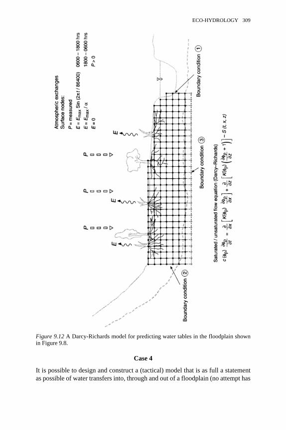
Case 4
It is possible to design and construct a (tactical) model that is as full a statementas possible of water transfers into, through and out of a floodplain (no attempt has
Figure 9.12 A Darcy-Richards model for predicting water tables in the floodplain shownin Figure 9.8.
ECO-HYDROLOGY 309
been made here at illustrating such a model). The main purpose of such a modelwould probably be for heuristic testing/numerical experimentation, as identifiedabove. However, such models must be tested in order to have any credibility. Inaddition to Darcy-Richards-type soil water fluxes, such a model could considermacropore flow and the role of larger soil pipes in transferring water through thefloodplain. To account for situations when the river is in flood or the water tablehas risen to the soil surface, an overland flow routine could be included.Evapotranspiration could be simulated using an energy balance model driven bydata collected using an automatic weather station (for an example of such anapplication see Spieksma et al., 1997).
Such a model would involve a considerable extension of the already verycomplex model shown in Figure 9.12 and, in view of earlier comments on theSHE model, would seem to be somewhat misguided, for it is unlikely that all ofthe processes could be measured accurately in the field in order to test the model.Indeed, it is unlikely that all of the processes included in the model are importantall the time in the real system. The very complexity of the model would alsorender it very difficult to use, and interpretation of ‘what if?’ testing would beconfounded by the problem of parameter variability; i.e. different credibleparameter sets could be used in a numerical experiment involving change of thefloodplain vegetation, but each set may give quite different results for the samevegetation change treatment. Thus it is difficult to see how the model could beused to make even basic statements about how the real system might behave.Franks and Beven (1997) have explored this issue in an analysis of a SVATmodel (TOPUP—Quinn et al., 1995) and conclude that the inclusion of a greaternumber of parameters/processes in a model leads to more input parameter setsthan could be considered realistic and consequently to greater uncertainty inmodel outputs or predictions. On the other hand, simpler models allow morerobust parameter estimation but have greater uncertainty associated with theirmore basic representation of certain processes.
Two options are open to the modeller when confronted with the problem ofwhich processes to include in a model and which to ignore. To illustrate this,consider the construction of a floodplain model but one in which the emphasis isnow on predicting water flow from the floodplain into the river rather than watertable rise and fall within the floodplain. The first approach could be called a top-down modelling approach. In this, the complex model, including all of the watertransfer processes likely to occur in a floodplain (Darcian soil water andgroundwater flow, pipe flow, overland flow, etc.), is constructed. A sensitivityanalysis of the model is then used to indicate which processes are most importantin controlling system behaviour. An example of such an analysis would involvealtering the values of hydraulic conductivity of the floodplain soil. The value ofK will affect groundwater flow rates through the soil according to Darcy’s law(equation (9.5)). If changes in the value of K had little impact on modelpredictions, i.e. the amount of water entering the river channel from thefloodplain, then K would be described as an insensitive parameter. It is probably
310 MODELLING
the case that for some modelling scenarios the model output would be sensitiveto the value of K, while in others it would be insensitive. If, for example, watertables in the floodplain are near the ground surface, ponding of water couldoccur on the floodplain shortly after rainfall, giving rise to overland flow andrapid water movement to the river channel. Under such conditions, the muchslower rates of flow associated with groundwater movement would beinsignificant. Thus the model would be insensitive to groundwater flow. Oneoutcome of such an analysis might be the construction of simpler models fordifferent flow scenarios. Thus a model that represents only overland flow couldbe used for predicting flow into the river during storms in late winter, whenwater tables might be expected to be near the ground surface. This simplermodel would then be tested with field observations. Kirkby et al. (1993: p. 172)have described this as a desirable outcome resulting from the use of complexmodels, although it is not clear whether they advocate constructing complexmodels in the first place in order to produce simpler models. The problem withthis approach is that several possible model scenarios could still produceessentially the same output. For example, groundwater flow to a dense networkof natural soil pipes could also produce rapid flows into the river from thefloodplain, and in this situation the model could be expected to be sensitive to Kbecause of its control on (shallow) groundwater flow into the soil pipes. Anadditional problem with this approach is that the sensitivity analysis of acomplex model would be difficult (perhaps impossible) to design and extremelytime-consuming.
An alternative, and possibly more efficient, way of proceeding (see below)could be called a bottom-up approach. In this approach, use is made of a limitedamount of field data before a model is constructed. For example, fieldmeasurements of river flow may indicate a very rapid response to late winterrainfall. Such a rapid response could arise only if water was conveyed rapidly tothe river channel. A reconnaissance field survey would give basic information onthe soil type and whether or not features such as soil pipes are present. If the soilwas clayey and soil pipes were absent it might be concluded that the floodplainwould be prone to winter waterlogging. From this fairly basic information itmight then be postulated that overland flow occurs in winter, when the watertable is very near the soil surface, and that this mechanism is the mainexplanation of the rapid increase in river discharge during and after winter rain.To test such a postulate, a simple model could be constructed. A sensible startingmodel would then be one in which the floodplain soil is treated as impermeableand rainfall is routed to the channel as overland flow; in other words, Darcianflow through the floodplain soil is ignored, even though it undoubtedly occurs. Inthis example, basic field information has been used to produce a simple modelthat can then tested with more detailed field data.
Both the top-down and bottom-up approaches can be used to construct simplemodels that retain the power of abstraction referred to by Gleick. Generally,however, the bottom-up approach is likely to prove the more efficient. In the
ECO-HYDROLOGY 311
above example this is clearly the case. The top-down approach involves theexpense of first constructing the complex model and then the problem ofdeciding which alternative sub-model to test first, assuming, of course, that thesensitivity analysis is not prohibitively expensive in terms of time or toodifficult. In addition, if basic field data have not been collected, it is possible thatboth of the alternatives (pipes and overland flow) may be inappropriate forsimulating flow to the river during winter, because it may be the case that rapidincreases in river discharge during and after rainfall never occur!
Does the blueprint work?
The blueprint based on the four questions above would appear to work in that, asis shown in the four cases, it minimises modelling effort and ‘forces’ modellersinto producing models that can be readily used and tested. In following theblueprint, pitfalls, such as developing complex physically based models in orderto predict water tables on a daily basis, are avoided. Essentially, the blueprintforces the modeller to consider developing the simplest model that meets her/hisrequirement, and therefore encourages efficiency in model development. Thequestion of testability is perhaps the most contentious in the blueprint, since,from the argument presented above, it is suggested that complex models aremore difficult to test than simple models and are consequently less useful. Hattonet al. (1997) reach a similar conclusion on testability and simplicity. Whilerecognising that complex models have a role to play in eco-hydrology, theysuggest that relatively simple, scale-independent models such as those developedby Eagleson (1978a-g) are a better way forward to understanding eco-hydrological behaviour in real systems, even though such models are based onphysically less meaningful ‘effective parameters’. Nevertheless, as has beenshown, testing can be difficult and can be subjective. Even with simple models,model predictions may not match the scale at which measurements can be taken(see Chapter 3), or the model output may not equate with a simple physicalparameter but rather a compound representation of several real-worldphenomena that is not capable of being easily measured/calculated. Similarly, inCase 2 it was suggested that deciding when a model is falsified is not astraightforward matter.
The issue of testability has also been discussed by Weiner (1995) who notesthat while most ecologists accept the need for testable theories, some centralmodels in ecology, such as the Lotka-Volterra population models, show littlesign of producing testable predictions. Some ecologists have even argued that theimportance of testability has been exaggerated (Fagerström, 1987, cited inWeiner, 1995) and that attributes such as the elegance and beauty of a model areequally important. Weiner (ibid.) dimisses such suggestions, noting that theywould lead to ‘a sort of nihilistic postmodern view of ecology where there is notruth, only stories, and the choice among stories is a question of individual taste(and power).’ Weiner concludes that the production of testable mathematical
312 MODELLING
models has to occupy the core of ecology, for without the production ofexplanatory and testable theories ecology will be little more than a discipline,like history, based on causal narratives. Testing is not easy, and currently mucheffort is expended in eco-hydrology on testing methodology (for example, GLUE—generalised likelihood uncertainty estimation: see Beven and Binley, 1992,and Freer et al., 1996). This must continue as a central theme within thediscipline. However, it is important to stress that an important part of such amethdology should be the production, in the first instance, of testable models.
Although the discussion here has been largely on (eco-)hydrological models, itis worth noting that workers in other areas of the environmental sciences havereached similar conclusions about simplicity/complexity and testability.Climatologists use models more than most environmental scientists. McGuffieand Henderson-Sellers (1997) place climate models into a scale of increasingcomplexity from one-dimensional energy balance models, which predict thevariation of Earth surface temperature with latitude, to general circulationmodels (GCMs), in which the three-dimensional nature of the atmosphere/oceansis simulated. Interestingly, the latter often contain SVAT sub-models which, asnoted earlier, can be regarded as ecohydrological. McGuffie and Henderson-Sellers (ibid.: p. 55) note that by 1980 most research funding went intoproducing complex three-dimensional models. They continue:
by the mid- to late 1980s a series of occurrences of apparently correctresults being generated for the wrong reason by these highly non-linear andhighly complex models prompted many modelling groups to movebackward, in an hierarchical sense, in order to try and isolate the essentialprocesses responsible for the results which are observed from the morecomplex models.
Later in their discussion they stress the need for developing models that are bothrelatively simple and capable of being tested. Similar conclusions have beenreached by Oreskes et al. (1994) in a review of modelling in the Earth sciences.
In conclusion, model construction is, or should be, the first stage of modeltesting. A model must be designed in a way that renders it capable of beingtested. To reiterate the point at the beginning of this section, a complex model,no matter how plausible, cannot be considered credible unless it has been testedor is capable of being tested. It is also important to stress again that testing isoften not a simple procedure that is used to declare that a model is ‘valid’ or‘invalid’. Deciding when a model gives a good representation of the real systemis both a qualitative and quantitative exercise, and often the conclusion reachedon model validity is partly a matter of opinion.
ECO-HYDROLOGY 313
MODELLING AND MATHEMATICS
As the focus of this chapter is mathematical models, it is appropriate to considerbriefly the role of mathematics in modelling. Many mathematicians aremodellers and have the same concerns as outlined in ‘A blueprint for bettermodelling?’ above. Mathematicians are also interested in developing solutions tothe equations used in models. For simple empirical models such as those shownin Case 1 (see Figure 9.10), the parameter values in the equation are derived fromfield data using statistical fitting methods. Once values of these parameters havebeen calculated, the equations can be used directly to calculate water tableelevation. With physically based models, the relationships between variables areusually non-linear and are posed as partial differential equations. Such equationscan be solved using flexible but approximate numerical solutions or, in a limitednumber of cases, traditional exact analytical methods. The difference betweenanalytical and numerical methods and their advantages and disadvantages areimportant considerations in modelling. Each approach is explained below.
Analytical (exact) solutions
An analytical solution to a problem results in a closed-form equation that can beused directly to obtain the value of a variable. If we consider the study ofinfiltration, the form of an analytical solution can be made clear. Other examplescould be used to illustrate the analytical approach, but these usually involveformidable mathematical detail. For this reason too, the derivation of theanalytical solution given below is not given.
A standard test in soil hydrology used for estimating the physical properties ofsurface layers of soil involves ponding water in a cylinder inserted into the soilsurface. The rate of water uptake by the soil, the infiltration rate, is measured as afunction of time. This rate of uptake depends on physical soil properties and thepotential gradient driving flow down through the soil profile, and it can beexpressed using empirical and physically based equations. An example of ananalytical infiltration equation derived from physical theory is that of Philip(1957), given by
(9.15)where i is infiltration rate (LT−1), A and B are constants that can, in principle, bederived from soil properties (A has dimensions of LT−1 and B has dimensions ofLT−0.5) and t is time (T). It can be seen that the equation can be used directly toobtain a value of infiltration rate providing that A, B and t are known. Theequation is thus described as closed-form.
Numerical (approximate) solutions
Some infiltration equations have been developed that describe the rate ofinfiltration as a function of the total amount of water stored in the soil and only
314 MODELLING
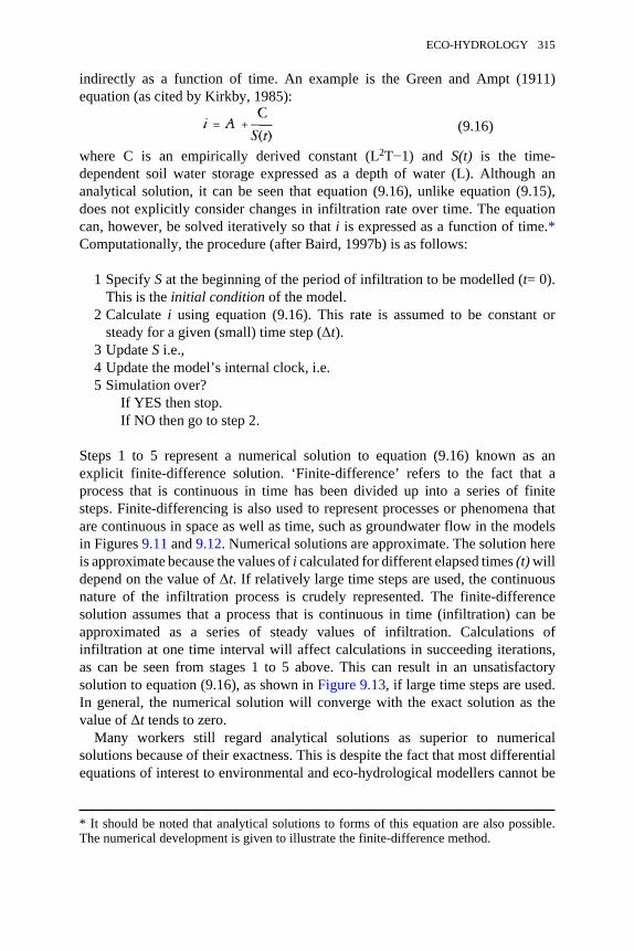
indirectly as a function of time. An example is the Green and Ampt (1911)equation (as cited by Kirkby, 1985):
(9.16)
where C is an empirically derived constant (L2T−1) and S(t) is the time-dependent soil water storage expressed as a depth of water (L). Although ananalytical solution, it can be seen that equation (9.16), unlike equation (9.15),does not explicitly consider changes in infiltration rate over time. The equationcan, however, be solved iteratively so that i is expressed as a function of time.*Computationally, the procedure (after Baird, 1997b) is as follows:
1 Specify S at the beginning of the period of infiltration to be modelled (t= 0).This is the initial condition of the model.
2 Calculate i using equation (9.16). This rate is assumed to be constant orsteady for a given (small) time step (∆t).
3 Update S i.e.,4 Update the model’s internal clock, i.e.5 Simulation over?
If YES then stop.If NO then go to step 2.
Steps 1 to 5 represent a numerical solution to equation (9.16) known as anexplicit finite-difference solution. ‘Finite-difference’ refers to the fact that aprocess that is continuous in time has been divided up into a series of finitesteps. Finite-differencing is also used to represent processes or phenomena thatare continuous in space as well as time, such as groundwater flow in the modelsin Figures 9.11 and 9.12. Numerical solutions are approximate. The solution hereis approximate because the values of i calculated for different elapsed times (t) willdepend on the value of ∆t. If relatively large time steps are used, the continuousnature of the infiltration process is crudely represented. The finite-differencesolution assumes that a process that is continuous in time (infiltration) can beapproximated as a series of steady values of infiltration. Calculations ofinfiltration at one time interval will affect calculations in succeeding iterations,as can be seen from stages 1 to 5 above. This can result in an unsatisfactorysolution to equation (9.16), as shown in Figure 9.13, if large time steps are used.In general, the numerical solution will converge with the exact solution as thevalue of ∆t tends to zero.
Many workers still regard analytical solutions as superior to numericalsolutions because of their exactness. This is despite the fact that most differentialequations of interest to environmental and eco-hydrological modellers cannot be
* It should be noted that analytical solutions to forms of this equation are also possible.The numerical development is given to illustrate the finite-difference method.
ECO-HYDROLOGY 315
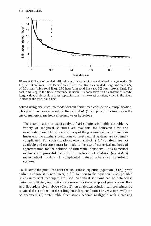
solved using analytical methods without sometimes considerable simplification.This point has been stressed by Remson et al. (1971: p. 56) in a treatise on theuse of numerical methods in groundwater hydrology:
The determination of exact analytic [sic] solutions is highly desirable. Avariety of analytical solutions are available for saturated flow andunsaturated flow. Unfortunately, many of the governing equations are non-linear and the auxiliary conditions of most natural systems are extremelycomplicated. For such situations, exact analytic [sic] solutions are notavailable and recourse must be made to the use of numerical methods ofapproximation for the solution of differential equations. Thus numericalmethods are powerful tools for the solution of realistic [my italics]mathematical models of complicated natural subsurface hydrologicsystems.
To illustrate the point, consider the Boussinesq equation (equation (9.12)) givenearlier. Because it is non-linear, a full solution to the equation is not possibleunless numerical techniques are used. Analytical solutions can be obtained ifcertain simplifying assumptions are made. For the example of groundwater flowin a floodplain given above (Case 2), an analytical solution can sometimes beobtained if (1) a function describing boundary condition 1 (river water level) canbe specified; (2) water table fluctuations become negligible with increasing
Figure 9.13 Rates of ponded infiltration as a function of time calculated using equation (9.16). A=0.3 cm hour−1; C=15 cm2 hour−1; S=1 cm. Rates calculated using time steps (∆t)of 0.01 hour (thick solid line); 0.05 hour (thin solid line) and 0.2 hour (broken line). Foreach time step in the finite difference solution, i is considered to be constant or steady.Large values of ∆t result in gross approximations to the exact solution, which in the figureis close to the thick solid line.
316 MODELLING
distance away from the river (towards the hill slope) i.e. and (3) a linearised formof the equation is used in which the saturated thickness of the aquifer is assumedconstant (d) rather than being the thickness of the local water table, i.e. theBoussinesq equation is replaced by the diffusion equation
(9.17)
The simplifications described in points (1) to (3) could sometimes lead to a muchpoorer representation of the real system than a full solution to the equation. Forexample, the saturated thickness of the aquifer can show great variabilitytemporally between summer and winter, violating condition (3). It is alsopossible that water table fluctuations at the boundary between the floodplain andthe hill slope will show considerable fluctuation, depending on the amount ofwater flowing through the hill-slope soils (violating conditions (2) and (3)).Finally, the river level boundary condition may be complex and may not beadequately described in the analytical solution. Thus, although an analyticalsolution will be exact, it will also be an exact approximation, because it is asolution to an approximation of the original differential equation to be solved.This is different from numerical approximations in that the approximation coniesbefore the solution. In such circumstances, which method is worse? Sometimes,exact analytical solutions are poorer representations of the real world. In theabove example, a number of numerical solutions to the full Boussinesq equationexist. Used properly, with carefully chosen time steps and sensible spatialdiscretisation of the floodplain, these solutions will involve very littleapproximation to the orginal equation and are thus to be preferred to exactanalytical approximations.
Analytical solutions are often regarded as more ‘elegant’ than numericalsolutions, presumably because of their exactness, and sometimes, if they arerelatively simple, they can reveal the structure of the solution to the differentialequation. However, as shown here, elegance in a solution to an equation is notalways important, whereas ‘elegance’ in the design and construction of a modelis, as noted earlier in this chapter, essential. The two should not be confused. Thesame holds true for choosing between numerical solutions. Many numericalmethods exist, and some are more elegant than others. For the modeller, it is notgenerally important which method is chosen as long as it is stable and can beshown to converge with the exact solution.
Mathematical onanism
A number of modellers indulge in ‘mathematical onanism’. If ‘onanism’ isdefined as ‘to stimulate the genital organs of (oneself or another) to achievesexual pleasure’ (Hanks, 1986), then mathematical onanism in eco-hydrologicalmodelling is ‘the search for new solutions to “governing” equations to achievemore publications’ (my definition). This definition is not meant as a slur on
ECO-HYDROLOGY 317

mathematicians. They are quite rightly concerned with how equations are solvedand the elegance and brevity of solution methods. However, some modellersseem more concerned with presenting new solutions (analytical solutions inparticular) to equations for which perfectly good solutions (often numerical)already exist. This is best left to mathematicians. Arguably, modellers shouldconcern themselves with whether a differential equation is an adequatedescription of the real system and with model design and testing. In a similarvein, Wilby (1997: p. 330) notes, ‘Rather than continuing the proliferation ofnew, “improved” models, greater understanding of processes could arise fromcritical assessments of existing theories.’ It is, then, disappointing to see so manypapers in the ecological and hydrological literature that do not address thesefundamental problems but rather present new solutions to equations. Examplesof mathematical onanism are abundant, as a look through recent volumes of anyinternational hydrological journal such as Journal of Hydrology and WaterResources Research will reveal. It is perhaps invidious to highlight examples ofthe practice. Nevertheless, two equations within hydrology seem to have beenthe subject of most mathematical onanism: the Darcy-Richards equation and theBoussinesq equation. Recent examples in just one journal (Journal ofHydrology) of new solutions to the Boussinesq equation when one did not appearto be needed are Guo (1997), Rai and Singh (1995), Ram et al. (1994),Govindaraju and Koelliker (1994) (see also Hogarth et al., 1997), and Su (1994).
SCALE, PROCESS, AND GOVERNING EQUATIONS INECO-HYDROLOGICAL MODELS
The issue of scale in eco-hydrology has already been dealt with in Chapter 3.However, some points relevant to the construction of eco-hydrological modelsare worth revisiting here. An increasing number of authors have givenprominence to the idea that nature is subject to different physical laws, or at leastdifferent forms of the same physical laws, at different scales (for a brief reviewsee Baird, 1997a; see also Turner, 1990, and Blöschl and Sivapalan, 1995). Yetthe idea that the mathematical description of a given phenomenon may dependon the scale at which it is being studied is not new. A classic example of howphysical laws are scale-dependent is groundwater flow through a porous medium.At many scales, Darcy’s law can be used to describe water flow through porousmedia. However, the law is a macroscopic law and applies only to flow through arepresentative volume of soil, called the representative elementary volume(REV), and not individual pores. The concept of the REV was introduced in aseminal paper by Hubbert (1940), although the term was apparently coined byBear (1972), who defined it as a volume of sufficient size that there are no longerany statistical variations in the value of a particular property (in this caseporosity) with the size of the element. The REV depends on the textural andstructural properties of the soil and is shown in Figure 9.14.
318 MODELLING

At the scale of an individual pore, water flow is virtually impossible todescribe mathematically unless the pore is conceptualised as a perfect cylinder.In cylindrical pores laminar flow can be described by the Hagan-Poiseuilleequation
(9.18)
where Q is pore discharge is the weight density of water r is the radius of thepore (L), µ is the dynamic viscosity of the fluid flowing through the pore is thehydrostatic pressure head acting on the face of the cylinder (L) (subscript 1 refersto the inflow point and 2 to the outflow), L is the length of the pore between 1and 2 (L), and is the angle of the pore from the horizontal (sin represents thegradient of the elevation head or potential). In ideal situations, equation (9.18)could be applied to larger scales than the individual pore. Flow through a porousmedium could be conceptualised as a bundle of capillary pores. The mathematicsof this approach are explained in Dingman (1984: pp. 294–296) and give rise toan equation analogous to Darcy’s law. Unfortunately, such an approach is notgenerally possible in real soils. Soil pores are not uniform, smooth tubes; theyare highly irregular in shape, and flow through them is limited by numerousconstrictions (Hillel, 1980). This microscopic complexity defies effectivedescription using laws similar to equation (9.18), and macroscopic laws that ignorethe microscopic detail are needed. There are upper limits to the applicability ofDarcy’s law. For example, Beven (1989) inter alia, has questioned whether it is
Figure 9.14 Definition of the representative elementary volume (REV). The REV in thiscase is V3. Source: Hubbert (1956) in Domenico and Schwartz (1990) (redrawn).Reproduced with permission of the American Institute of Mining, Metallurgical andPetroleum Engineers.
ECO-HYDROLOGY 319
appropriate to use Darcy’s law in finite-difference models with computationalcells with dimensions of tens or hundreds of metres across. Is there any meaningin a hydraulic gradient calculated between two large cells when in the real systemthe gradient is changing significantly over much smaller scales, partly due to the(relatively small-scale) heterogeneity of the real system?
The problem of whether laws developed for small-scale laboratory studies canbe applied at larger scales has also been discussed recently by Hatton et al.(1997). They question whether the bottom-up approach of applying small-scalephysical laws to hill slopes or event catchments is appropriate. Nevertheless, theyappear to suggest that small-scale laws such as Darcy’s law can be used at largerscales, providing that it is recognised that the law no longer has the same physicalmeaning as it does when applied at the laboratory scale. Thus, although thegoverning equation may have the same form across scales, it uses scale-dependent effective parameters and thus is not the same law at every scale. Thisis an argument previously articulated by Smith et al. (1994) (see also Baird,1997a).
Another example of the importance of scale in conceptualising systembehaviour is (evapo)transpiration. Jarvis and McNaughton (1986) note that plantphysiologists and ecologists have suggested that stomata play a dominant role inregulating the amount of water transpired by vegetation, whilemicrometeorologists have tended to stress the role played by energy supply toplants. Jarvis and McNaughton set about answering the question ‘To what extentdo stomata control transpiration?’ and show that the answer depends on the scaleof investigation. At the scale of the leaf or individual plant, transpiration isdetermined by vapour pressure deficit and stomatal processes, whereas atregional scales it is controlled by net radiation (for a detailed explanation of thissee the original paper or Chapter 2). In the example of groundwater flow thebasic processes describing the phenomenon are the same regardless of whetherDarcy’s law or Poiseuille’s equation are being used. In the case ofevapotranspiration, it is the governing processes as well as the mathematicaldescription that change depending on the scale of investigation.
The message from this brief section is clear: the suitability of a model fordescribing a particular phenomenon will depend on the scale at which it is beingapplied. This point should always be uppermost in the modeller’s mind whenconstructing a model and choosing which processes to include in a description ofsystem behaviour.
THE VALUE OF MATHEMATICAL MODELS
This chapter has, in places, tended to dwell on the deficiencies in existing modelsand approaches to modelling while giving less attention to the value ofmathematical models. Therefore, it is worth re-emphasising that mathematicalmodels are an essential tool in many branches of eco-hydrology. In many cases(i.e. with physically based models), models are our formal encodings of theories
320 MODELLING
and if coded properly allow the theories to be tested and the discipline toadvance. Without testing, a theory lacks credibility. It is not enough simply tosuggest that the theory appears to represent the essential patterns of a system;this must be shown to be the case. Most science is quantitative and predictive(although see the impassioned and well-argued plea for descriptive science givenby Gould, 1989). Indeed, prediction is often used to test the validity of ourunderstanding of nature. Assessing the value of quantitative prediction is noteasy and involves subjectivity; science is, after all, partly a social process. It is,however, far easier to compare two sets of data, one modelled, the othermeasured, than it is to assess the validity of a nebulous, qualitative ‘prediction’or a feeling that a model or theory captures in some way the essential dynamicsof a system. In addition, although empirical models have a place within eco-hydrology, without theory testing there is the danger that eco-hydrology willbecome a discipline that deals with site-specific causal narratives (Weiner, 1995)rather than true explanations of process. Thus physically based mathematicalmodels will remain fundamental tools of researchers in eco-hydrology, but theymust be used sensibly.
ACKNOWLEDGEMENTS
This chapter has benefited enormously from the critical comments on an earlierversion of the manuscript of George Hornberger, Rob Wilby and SimonGaffney. As usual, any errors or inconsistencies remain the fault of the author.The diagrams were prepared by Paul Coles and Graham Allsopp of CartographicServices at the Department of Geography, University of Sheffield.
REFERENCES
Abbott, M.B., Bathurst, J.C., Cunge, J.A., O’Connell, P.E. and Rasmussen. J. (1986a) Anintroduction to the European Hydrological System—Système HydrologiqueEuropéen, ‘SHE’. 1: History and philosophy of a physically-based, distributedmodelling system, Journal of Hydrology 87:45–59.
Abbott, M.B., Bathurst, J.C., Cunge, J.A., O’Connell, P.E. and Rasmussen. J. (1986b) Anintroduction to the European Hydrological System—Système HydrologiqueEuropéen, ‘SHE’. 2: Structure of a physically-based, distributed modelling system,Journal of Hydrology 87:61–77.
Addiscott, T.M., and Wagenet, R.J. (1985) Concepts of solute leaching in soils: a reviewof modelling approaches, Journal of Soil Science 36:411–424.
Armstrong, A.C. (1988) Modelling rainfall/watertable relations using linear responsefunctions, Hydrological Processes 2:383–389.
Baird, A.J. (1997a) Continuity in hydrological systems, in R.L.Wilby (ed.) ContemporaryHydrology: Towards Holistic Environmental Science, Chichester: Wiley, pp. 25–58.
ECO-HYDROLOGY 321
Baird, A.J. (1997b) Overland flow generation and sediment mobilisation by water, inD.S.G.Thomas (ed.) Arid Zone Geomorphology: Process, Form and Change inDrylands, Chichester: Wiley, 713 pp.
Bathurst, J.C. (1986) Physically-based distributed modelling of an upland catchment usingthe Système Hydrologique Européen, Journal of Hydrology 87: 79–102.
Bathurst, J.C., Kilsby, C. and White, S. (1996) Modelling the impacts of climate and land-use change on basin hydrology and soil erosion in Mediterranean Europe, in Brandt,C.J. and Thornes, J.B. (eds) Mediterranean Desertification and Land Use,Chichester: Wiley, pp. 355–387.
Bear, J. (1972) Dynamics of Fluids in Porous Media, Elsevier, New York, 764 pp.Beven, K. (1985) Distributed models, in M.G.Anderson and T.P.Burt (eds) Hydrological
Forecasting, Chichester: Wiley, pp. 405–435.Beven, K. (1989) Changing ideas in hydrology—the case of physically based models,
Journal of Hydrology 137:149–163.Beven, K. (1996) Equifinality and uncertainty in geomorphological modelling, in
B.L.Rhoads and C.E.Thorn (eds) The Scientific Nature of Geomorphology:Proceedings of the 27th Binghamton Symposium in Geomorphology, held 27–29September 1996, Chichester: Wiley.
Beven, K. and Binley, A.M. (1992) The future of distributed models: model calibrationand uncertainty prediction, Hydrological Processes 6:279–298.
Blackie, J.R. and Eeles, C.W.O. (1985) Lumped catchment models, in M.G. Andersonand T.P.Burt (eds) Hydrological Forecasting, Chichester: Wiley, pp. 311–345.
Blöschl, G. and Sivapalan, M. (1995) Scale issues in modelling: a review, in J.D. Kalmaand M.Sivapalan (eds) Scale Issues in Hydrological Modelling, Chichester: Wiley,pp. 71–88.
Boussinesq, J. (1904) Recherches théoriques sur l’écoulement des nappes d’eau infiltréesdan le sol et sur le débit des sources, Journal de Mathématiques Pares et Appliquées10:5–78.
Box, G.E.P. and Jenkins, G.M. (1976) Time Series Analysis: Forecasting and Control,San Francisco: Holden-Day.
Busch, D.E., Loftus, W.F., and Bass, O.L. Jr (1998) Long-term hydrologic effects onmarsh plant community structure in the southern Everglades, Wetlands 18: 230–241.
Campbell, G.S. (1981) Fundamentals of radiation and temperature relations, inEncyclopedia of Plant Physiology New Series Vol. 12A, New York: Springer-Verlag,pp. 11–40.
Childs, E.G. and Youngs, E.G. (1968) Note on the paper ‘Explanation of paradoxes inDupuit-Forchheimer seepage theory’, by Don Kirkham, Water Resources Research 4:219–220.
Dingman, S.L. (1984) Fluvial Hydrology, New York: Freeman, 383 pp.Dingman, S.L. (1994) Physical Hydrology, New York: Macmillan.Domenico, P.A. and Schwartz, F.W. (1990) Physical and Chemical Hydrogeology, New
York: Wiley, 824 pp.Eagleson, P.S. (1978a) Climate, soil, and vegetation. 1. Introduction to water balance
dynamics, Water Resources Research 14:705–712.Eagleson, P.S. (1978b) Climate, soil, and vegetation. 2. The distribution of annual
precipitation derived from observed storm sequences, Water Resources Research 14:713–721.
322 MODELLING
Eagleson, P.S. (1978c) Climate, soil, and vegetation. 3. A simplified model of soil watermovement in the liquid phase, Water Resources Research 14:722–730.
Eagleson, P.S. (1978d) Climate, soil, and vegetation. 4. The expected value of annualevapotranspiration, Water Resources Research 14:731–739.
Eagleson, P.S. (1978e) Climate, soil, and vegetation. 5. A derived distribution of stormsurface runoff, Water Resources Research 14:741–748.
Eagleson, P.S. (1978f) Climate, soil, and vegetation. 6. Dynamics of the annual waterbalance, Water Resources Research 14:749–764.
Eagleson, P.S. (1978g) Climate, soil, and vegetation. 7. A derived distribution of annualwater yield, Water Resources Research 14:765–776.
Eagleton, T. (1986) The critic as clown, in Eagleton, T., Against the Grain: Essays 1975–1985, London: Verso, p. 149.
Fagerström, T. (1987) On theory, data and mathematics in ecology, Oikos 50: 258–261.Feddes, R.A., Kabat, P., van Bakel, P.J.T., Bronswijk, J.J.B. and Halbertsma, J. (1988) Modelling soil water dynamics in the unsaturated zone—state of the art, Journal
of Hydrology 100:69–111.Franks, S.W. and Beven, K.J. (1997) Bayesian estimation of uncertainty in land surface-
atmosphere flux predictions, Journal of Geophysical Research 102 D20:23991–23999.
Franks, S.W., Beven, K.J., Quinn, P.F. and Wright, I.R. (1997) On the sensitivity of soil-vegetation-atmosphere transfer (SVAT) schemes: Equifinality and the problem ofrobust calibration , Agricultural and Forest Meteorology 86:63–75.
Freer, J., Beven, K.J. and Ambroise, B. (1996) Bayesian estimation of uncertainty inrunoff prediction and the value of data: an application of the GLUE approach, WaterResources Research 32:2161–2173.
Freeze, R.A. and Cherry, J.A. (1979) Groundwater, Englewood Cliffs, New Jersey:Prentice-Hall, 604 pp.
Gardner, M. (1989) Foreword, in R.Penrose, The Emperor’s New Mind: ConcerningComputers, Minds, and the Laws of Physics, Oxford: Oxford University Press.
Gardner, W.R. (1957) Some steady-state solutions of the unsaturated moisture flowequation with application to evaporation from a water table, Soil Science 85:228–232.
Gillman, M. and Hails, R. (1997) An Introduction to Ecological Modelling: PuttingPractice into Theory, Oxford: Blackwell, 202 pp.
Gilvear, D.J., Andrews, R., Tellam, J.H., Lloyd, J.W. and Lerner, D.N. (1993)Quantification of the water balance and hydrogeological processes in the vicinity of asmall groundwater-fed wetland, East Anglia, UK, Journal of Hydrology 144:311–334.
Gilvear, D.J., Sadler, P.J.K., Tellam, J.H. and Lloyd, J.W. (1997) Surface water processesand groundwater flow within a hydrologically complex floodplain wetland, NorfolkBroads, UK, Hydrology and Earth System Sciences 1:115–135.
Gleick, J. (1988) Chaos: Making a New Science, London: Heinemann.Goldsmith, F.B., Harrison, C.M. and Morton, A.J. (1986) Description and analysis of
vegetation, in Moore, P.D. and Chapman, S.B. (eds) Methods in Plant Ecology,Oxford: Blackwell, pp. 437–524.
Gould, S.J. (1989) Wonderful Life: The Burgess Shale and the Nature of History, London:Hutchinson Radius, 347 pp.
ECO-HYDROLOGY 323

Govindaraju, R.S. and Koelliker, J.K. (1994) Applicability of linearized Boussinesqequation for modeling bank storage under uncertain aquifer parameters, Journal ofHydrology 157:349–366.
Grayson, R.B., Moore, I.D. and McMahon, T.A. (1992) Physically based hydrologicmodeling. 2. Is the concept realistic? Water Resources Research 28: 2659–2666.
Green, W.H. and Ampt, G.A. (1911) Studies on soil physics. 1. The flow of water throughsoils. Journal of Agricultural Science 4.1:1–24.
Guo, W. (1997) Transient groundwater flow between reservoirs and water-table aquifers,Journal of Hydrology 195:370–384.
Hanks, P. (ed.) (1986) Collins English Dictionary, Glasgow: Collins, 1771 pp. Hatton, T.J., Salvucci, G.D. and Wu, H.I. (1997) Eagleson’s optimality theory of an
ecohydrological equilibrium: quo vadis? Functional Ecology 11:665–674.Hill, M.O. (1979) DECORANA, a FORTRAN Program for Detrended Correspondence
Analysis and Reciprocal Averaging, Ithaca, New York: Microcomputer Power.Hillel, D. (1977) Computer Simulation of Soil Water Dynamics; A Compendium of Recent
Work, Ottawa: International Development Research Center.Hillel, D. (1980) Fundamentals of Soil Physics, New York: Academic Press.Hillel, D., Talpaz, H. and Van Keulen, H. (1976) Macroscopic-scale model of water
uptake by a non-uniform root system and of water and salt movement in the soilprofile, Soil Science 121:242–255.
Hogarth, W.L., Govindaraju, R.S., Parlange, J.-Y., and Koelliker, J.K. (1997) LinearisedBoussinesq equation for modelling bank storage—a correction, Journal of Hydrology198:377–385.
Holling, C.S. (1966) The strategy of building models in complex ecological systems, inK.E.F.Watt (ed.) Systems Analysis in Ecology, New York: Academic Press.
Hubbert, M.K. (1940) The theory of groundwater motion, Journal of Geology 48:785–944.
Hubbert, M.K. (1956) Darcy’s law and the field equations of the flow of undergroundfluids, Transactions of the American Institute of Mining, Metallurgical andPetroleum Engineers 207:222–239.
Jarvis, P.G. and McNaughton, K.G. (1986) Stomatal control of transpiration: scaling upfrom the leaf to the region, Advances in Ecological Research 15:1–49.
Kennedy, B.A. (1985) Indeterminancy, in A.Goudie (ed.) The Encyclopaedic Dictionaryof Physical Geography, Oxford: Blackwell, 528 pp.
Kirkby, M.J. (1985) Infiltration, in A.Goudie (ed.) The Encyclopaedic Dictionary ofPhysical Geography, Oxford: Blackwell, 528 pp.
Kirkby, M.J., Baird, A.J., Diamond, S.M., Lockwood, J.G., McMahon, M.L., Mitchell,P.L., Shao, J., Sheehy, J.E., Thornes, J.B. and Woodward, F.I. (1996) The Medalusslope catena model: a physically based process model for hydrology, ecology andland degradation interactions, in Brandt, C.J. and Thornes, J.B. (eds) MediterraneanDesertification and Land Use, Chichester: Wiley, pp. 303–354.
Kirkby, M.J., Naden, P.S., Burt, T.P. and Butcher, D.P. (1993) Computer Simulation inPhysical Geography, Chichester: Wiley.
Kirkham, D. (1967) Explanation of paradoxes in Dupuit-Forchheimer seepage theory,Water Resources Research 3:609–622.
May, R.M. (1973) Stability and Complexity in Model Ecosystems, New Jersey: PrincetonUniversity Press.
324 MODELLING
McGuffie, K. and Henderson-Sellers, A. (1997) A Climate Modelling Primer, Chichester:Wiley, 253 pp.
McWhorter, D.B. and Sunada, D.K. (1977) Ground-Water Hydrology and Hydraulics,Fort Collins: Water Resources Publications.
Monteith, J.L. (1973) Principles of Environmental Physics, London: Edward Arnold.Mulligan, M. (1996a) Modelling hydrology and vegetation change in a degraded semi-
arid environment, unpublished PhD thesis, King’s College, University of London. Mulligan, M. (1996b) Modelling the complexity of land surface response to climatic
variability in Mediterranean environments, in Anderson, M.G. and Brooks, S.M.(eds) Advances in Hillslope Processes, Chichester: Wiley, pp. 1099–1149.
Murray, W.A. and Monkmeyer, P.L. (1973) Validity of Dupuit-Forchheimer equation.Journal of the Hydraulics Division (American Society of Civil Engineers) 97(HY9):1573–1583.
Nielsen, D.R., Biggar, J.W. and Erh, K.T. (1973) Spatial variability of field measured soilwater properties, Hilgardia 42:215–259.
Oreskes, N., Shrader-Frechette, K. and Belitz, K. (1994) Verification, validation andconfirmation of numerical models in the earth sciences, Science 263:641–646.
Penman, H.L. (1948) Natural evaporation from open water, bare soil and grass,Proceedings of the Royal Society, Series A 193:120–145.
Philip, J.R. (1957) The theory of infiltration. 4: Sorptivity and algebraic infiltrationequations, Soil Science 84:257–264.
Popper, K. (1968) Conjectures and Refutations: The Growth of Scientific Knowledge,New York: Harper & Row.
Popper, K. (1972) Objective Knowledge: An Evolutionary Approach, Oxford: OxfordUniversity Press.
Quinn, P.F., Beven, K.J. and Culf, A. (1995) The introduction of macroscale hydrologicalcomplexity into land surface-atmosphere transfer models and the effect of planetaryboundary layer development, Journal of Hydrology 166:421–444.
Ragab, R. and Cooper, J.D. (1993) Variability of unsaturated zone water transportparameters: implications for hydrological modelling. 1: In situ measurements.Journal of Hydrology 148:109–132.
Rai, S.N. and Singh, R.N. (1995) Two dimensional modelling of water table fluctuation inresponse to localised transient recharge, Journal of Hydrology 167: 167–174.
Ram, S., Jaiswal, C.S. and Chauhan, H.S. (1994) Transient water table rise with canalseepage and recharge, Journal of Hydrology 163:197–202.
Remson, I., Hornberger, G.M. and Molz, F.J. (1971) Numerical Methods in SubsurfaceHydrology with an Introduction to the Finite Element Method, New York: Wiley,389 pp.
Rennolls, K., Carnell, R. and Tee, V. (1980) A descriptive model of the relations betweenrainfall and soil water table, Journal of Hydrology 47:103–114.
Richards, L.A. (1931) Capillary conduction of liquids through porous mediums, Physics 1:318–333.
Rogowski, A.S. (1972) Watershed physics: soil variability criteria, Water ResourcesResearch 8:1015–1023.
Smith, R.E., Goodrich, D.R., Woolhiser, D.A. and Simanton, J.R. (1994) Comment on‘Physically based hydrologic modeling. 2. Is the concept realistic?’ by R.B. Grayson,I.D.Moore, and T.A.McMahon, Water Resources Research 30:851–854.
ECO-HYDROLOGY 325
Spieksma, J.F.M., Moors, E.J., Dolman, A.J. and Schouwenaars, J.M. (1997) Modellingevaporation from a drained and rewetted peatland, Journal of Hydrology 199:252–271.
Su, N. (1994) A formula for computation of time-varying recharge of groundwater,Journal of Hydrology 160:123–135.
Turner, M.G. (1990) Spatial and temporal analysis of landscape patterns, LandscapeEcology 4:21–30.
van Elburg, H., Engelen, G.B. and Hemker, C.J. (1991) FLOWNET Version 5.1: User’sManual. Microcomputer Modeling of Two-dimensional Steady State GroundwaterFlow in a Rectangular Heterogeneous Anisotropic Section of the Subsoil,Amsterdam: Institute of Earth Sciences, Free University of Amsterdam.
Verburg, K., Ross, P.J. and Bristow, K.L. (1996) SWIMv2.1 User Manual, DivisionalReport of the CSIRO Division of Soils No. 130, 107 pp.
Viera, S.R., Nielsen, D.R. and Biggar, J.W. (1981) Spatial variability of field-measuredinfiltration rates, Proceedings of the Soil Science Society of America 45: 1040–1048.
Wang, H.F. and Anderson, M.P. (1982) Introduction to Groundwater Modelling: FiniteDifference and Finite Element Methods, San Diego: Academic Press, 237 pp.
Ward, R.C. and Robinson, M. (1990) Principles of Hydrology, third edition, London:McGraw-Hill.
Warrick, A.W. and Nielsen, D.R. (1980) Spatial variability of soil physical properties inthe field, in D.Hillel (ed.) Applications of Soil Physics, London: Academic Press.
Wassen, M.J., van Diggelen, R., Wolejko, L. and Verhoeven, J.T.A. (1996) A comparisonof fens in natural and artificial landscapes, Vegetatio 126:5–26.
Watts, G. (1997) Hydrological Modelling in Practice, in R.L.Wilby (ed.) ContemporaryHydrology: Towards Holistic Environmental Science, Chichester: Wiley,pp. 151–193.
Weiner, J. (1995) On the practice of ecology, Journal of Ecology 83:153–158.Wicks, J.M. and Bathurst, J.C. (1996) SHESED: A physically based, distributed erosion
and sediment yield component for the SHE hydrological modelling system, Journalof Hydrology 174:213–238.
Wilby, R.L. (1997) Beyond the river catchment, in R.L.Wilby (ed.) ContemporaryHydrology: Towards Holistic Environmental Science, Chichester: Wiley,pp. 317–346.
326 MODELLING
10THE FUTURE OF EGO-HYDROLOGY
Robert L.Wilby
INTRODUCTION
One of the defining social themes of the decade has been ecologicalawareness. Consequently, ecology now stands at the interfacebetween science and public policy. Pressure groups, citizens, andpolicy-makers can draw on ecological research to form opinions onthe ‘big questions’ facing the planet: what to do about climatechange, biodiversity, population control, and other pressing matters.So the issue of how ecologists gather information, and how thatinformation can be applied, becomes tremendously important.
Gallagher et al. (1995)
The same could also be said of hydrology. Water, in the form of vapour, liquid,snow and ice, is critical to the present functioning and future changes in theglobal climate. Water-borne nutrients, soil moisture deficits and surpluses areoften limiting factors affecting the temporal and spatial dynamics of vegetationsystems. Water resources for domestic supplies, irrigation, navigation andindustry are subject to increasing competition as populations and economiescontinue to grow. Water is involved in many human-induced problems, such asaccelerated soil erosion, environmental pollution and ecosystem degradation. Sothe issue of how hydrologists gather information, and how that information canbe applied, becomes tremendously important.The preceding chapters on plant-water relations have demonstrated howhydrology can be applied within ecology, and how knowledge of ecology isimportant to our understanding of hydrological processes. Three underlyingthemes emerged, namely the importance of considering scale effects, the valueof well-designed field and laboratory experiments, and the need for appropriatemathematical models in eco-hydrological research. As Tyree (Chapter 2) andWilby and Schimel (Chapter 3) indicated, plant-water relations can be consideredat a multitude of scales, ranging from individual cells in plants to the planetary
scale. Indeed, the issue of scale is receiving much attention as hydrologists seekto unify processes operating at different temporal and spatial scales (cf. Blöschl,1997), and as ecologists seek to formulate a new understanding of multi-scalebiotic and abiotic inter-connections (cf. Root and Schneider, 1995).
Chapters 4 to 8 examined the dominant plant-water relations operating withinspecific environments. A common theme emerging from all the chapters is thedifficulty of isolating causes and effects in plant-water relationships. Forexample, Wainwright, Mulligan and Thornes (Chapter 4) demonstrated that inarid and semi-arid environments the distribution of plants has a profound effecton overland flow processes and erosion. The focusing of overland flow in inter-shrub areas leads to the development of desert pavements, a process, perhapstriggered by overgrazing, that is hydrologically self-perpetuating and ultimatelyresults in the replacement of grassland by scrub. Wheeler (Chapter 5) discussedthe elusive definition of ‘typical’ wetland species, emphasising the hydrologicalcontrols exerted on plant assemblages. Although the ‘wetness’ processesaffecting individual plant growth are well understood from laboratoryexperiments, it was shown that plant communities are responsive to fluctuatingwater levels, that individual species’ ranges are often broad and, because of this,it is often difficult to specify exact environmental preferences. Roberts(Chapter 6) demonstrated on the one hand the role of plants in the storage androuting of water movement via the canopy and soils, and on the other, theregulation in some cases, of forest evapotranspiration by soil moisture variations.
The importance of considering dynamic, three-dimensional hydrologicalcontrols on plants was discussed with reference to streams and rivers in Largeand Prach (Chapter 7). It was demonstrated that ephemeral and subsurface flowscomplicate the concept of the river corridor, and that the two-way exchange ofwater and nutrients between the river and floodplain is critical to the regulation ofplant communities in these ecotones. Similarly, Wetzel (Chapter 8) showed thatthe productivity of emergent macrophytes at the land-water interface of lakemargins shapes, and is shaped by, hydrological processes regulating nutrient andsediment stores. Plants in lakes are effectively a ‘metabolic wick’, altering thepatterns of flow, rates of evapotranspiration and water balances of theecosystem.
Finally, Baird (Chapter 9) critically examined the use and abuse ofmathematical models as a tool for representing the complex eco-hydrologicalprocesses discussed in the previous chapters. It was shown that it is preferable .to apply simpler models, in which the key processes are well prescribed andappropriate, than over-parameterised ‘replicas’ of the real system. This is due tothe problems associated with parameter identifiability and the equifinality ofmodel results that can arise when a reductionist approach to model building isemployed.
As the following sections indicate, mathematical models will continue tofigure prominently as a means of exploring plant-water relations in a multitudeof terrestrial environments and across a wide spectrum of temporal and spatial
328 THE FUTURE OF ECO-HYDROLOGY

scales. However, this presupposes the existence of carefully designed field andlaboratory experiments, as well as the assimilation of new data types, inparticular from remote-sensing technology. Furthermore, there is considerablescope for coordinated fieldwork campaigns, and for the intercomparison of modelsusing common data sets. Increasingly, human impacts on eco-hydrologicalprocesses are attaining global dimensions: these concerns are reflected by theongoing development of integrated atmosphere-biosphere-hydrosphere models,and by a growing appreciation of the significance of plant-water-climatefeedbacks. At the landscape scale, field experimentation and modeldevelopments could herald a new era in hydrology: an age in which eco-hydrological processes may be deliberately manipulated in order to bring aboutenvironmental restoration, remediation or recovery. But before this can happenthere are a number of environmental uncertainties that require our urgentattention.
EMBRACING ENVIRONMENTAL UNCERTAINTIES
There are few if any terrestrial and, to a lesser extent, marine environments thathave not been marked by the human fingerprint: all organisms modify theirenvironment, and humans are no exception. As Vitousek et al. (1997) point out,human activities have transformed the Earth’s land surface, reduced biodiversity,altered marine ecosystems (particularly at coastal margins), regulated most majorrivers, modified biogeochemical cycles and changed the composition of soils,water and the atmosphere (Figure 10.1). In other words, there are few, if any,pristine environments or landscapes for eco-hydrologists to study. Therefore, anyserious analysis of the functioning of plant-water systems should incorporatehuman factors. Fortuitously, hydrology has a long history of pure and appliedresearch (James, 1991) and is well placed to address the ‘big questions’ of thetwenty-first century, because hydrological processes transcend traditionaldisciplinary divides and provide scope for the development of a holisticenvironmental science (Wilby, 1997). The challenge that confronts us now is toinfuse eco-hydrological research with the same principles.
Inevitably, the significance of human impacts and the Earth’s capacity tosupport human populations is determined both by natural constraints and bysocietal choices concerning economics, politics, culture and demography(Cohen, 1995). A good example of the inherent uncertainty surrounding thesechoices is the recent debate concerning economic and environmental options forthe stabilisation of atmospheric greenhouse gas concentrations, anecessary action to prevent or reduce dangerous anthropic interference with theclimate system. By viewing the stabilisation issue as a carbon budget allocationproblem, Wigley et al. (1996) argue that emission reductions should be deferredfor economic and technical reasons. In the medium term, both the stabilisationpathway and climatic response are highly uncertain, with concomitantimplications for global ecosystems. Since future economic and technological
ECO-HYDROLOGY 329
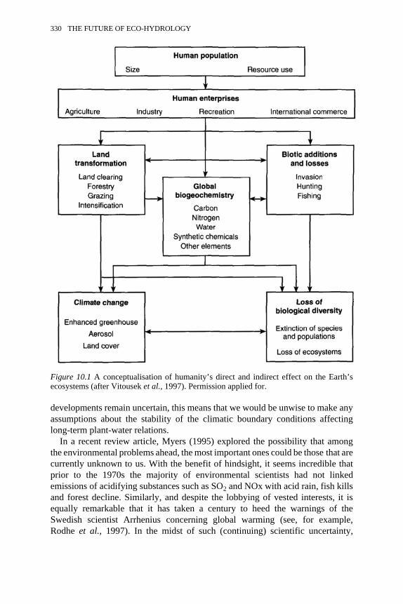
developments remain uncertain, this means that we would be unwise to make anyassumptions about the stability of the climatic boundary conditions affectinglong-term plant-water relations.
In a recent review article, Myers (1995) explored the possibility that amongthe environmental problems ahead, the most important ones could be those that arecurrently unknown to us. With the benefit of hindsight, it seems incredible thatprior to the 1970s the majority of environmental scientists had not linkedemissions of acidifying substances such as SO2 and NOx with acid rain, fish killsand forest decline. Similarly, and despite the lobbying of vested interests, it isequally remarkable that it has taken a century to heed the warnings of theSwedish scientist Arrhenius concerning global warming (see, for example,Rodhe et al., 1997). In the midst of such (continuing) scientific uncertainty,
Figure 10.1 A conceptualisation of humanity’s direct and indirect effect on the Earth’secosystems (after Vitousek et al., 1997). Permission applied for.
330 THE FUTURE OF ECO-HYDROLOGY

Myers (1995) suggests that we might be able to anticipate two types ofenvironmental unknown, namely discontinuities and synergisms. Both have thepotential to introduce significant and unforeseen feedbacks, which may be highlynon-linear.
Environmental discontinuities arise when accumulating stresses on anecosystem attain a critical threshold, at which point the period of no (apparent)injury is replaced by a dramatic shift in system structure or behaviour. Forexample, systematic changes in terrestrial biota resulting from habitat conversionand land-use change reduce genetic and species diversity, leading to ahomogenisation of global biota (Chapin et al., 1997). This may have seriousimplications, since biodiversity regulates ecosystem function and stability(McGrady-Steed et al., 1997). One of the least studied and understoodbiodiversity relationships is between soil biota (approximately 175,000 knownspecies) and ecosystem processes in freshwater sediments (Palmer et al., 1997).Yet these species provide a number of important ecosystem services (e.g.decomposition of organic matter, nutrient cycling, bioturbation, suppression ofsoil-borne diseases and pests, etc.), which are at risk from intensive agriculture,forest disturbance and pollution (Brussaard et al., 1997). Experimental evidencefrom microbial microcosms shows that ecosystem respiration, biomass anddensity measures become more predictable as biodiversity increases, and thatredundancy (i.e. multiple species per functional group) is a valuable commodity(Naeem and Li, 1997). For example, Tilman and Downing (1994) demonstratedthat the presence of drought-tolerant species in diverse grasslands maintainshigher productivity under drought conditions than grasslands with lowerdiversity. This is because high diversity within functional groups also providesgreater resilience in response to environmental change, since decreases in theabundance of one species will be compensated for by increases in otherfunctionally similar species.
Therefore, the fewer species there are in any assemblage, the more likely it isthat further extinctions will dramatically affect ecosystem processes. Inparticular, the introduction or removal of predators or diseases that have large‘keystone’ effects can result in ecosystem responses that are substantially greaterthan might have been anticipated from the biomass of the species alone. Forexample, the removal by humans of elephants or other keystone herbivores canlead to the encroachment of woody plants into savannahs; conversely, theconcrentration of high densities of elephants in national parks can result insignificant environmental degradation (Chapin et al., 1997). Thus subtle changesin ecosystem resource dynamics, trophic structure or disturbance regimes canultimately have major implications for plant-water processes.
Nonetheless, threshold or discontinuity effects are thought to characterise bothnatural and human-impacted systems. For example, the climate system is knownto have more than one equilibrium state, and intrinsic or extrinsic perturbationscan trigger rapid transitions between states. Evidence from Greenland ice coresand deep ocean sediment records suggest that although the Holocene has been
ECO-HYDROLOGY 331
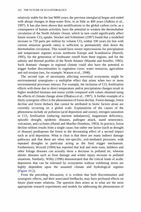
relatively stable for the last 9000 years, the previous interglacial began and endedwith abrupt changes in deep-water flow, in as little as 400 years (Adkins et al.,1997). It has also been shown that modifications to the global carbon cycle, as aconsequence of human activities, have the potential to weaken the thermohalinecirculation of the North Atlantic Ocean, which in turn could significantly affectfuture oceanic CO2 uptake. Stocker and Schmittner (1997) found that a modelledincrease to 750 parts per million by volume CO2 within 100 years (in line withcurrent emission growth rates) is sufficient to permanently shut down thethermohaline circulation. This would have severe repercussions for precipitationand temperature regimes across northwest Europe and Scandinavia (Hurrell,1995), for the generation of freshwater runoff from these regions, and for thesalinity and thermal profiles of the North Atlantic (Manabe and Stouffer, 1995).Such dramatic changes in regional climate could also have the potential totrigger further discontinuities in vegetation cover, water resources, agricultureand soil erosion (see, for example, Watson et al., 1998).
The second type of uncertainty affecting terrestrial ecosystems might beenvironmental synergisms—a multiplier effect that arises when two or moreenvironmental processes interact. For example, the inclusion of CO2 fertilisationeffects with those due to direct temperature and/or precipitation changes result inhigher modelled biomass and maize yields compared with values obtained usingthe effects of climate change alone (Dhakwa et al., 1997). A further example of alikely synergistic effect is the phenomenon of forest decline. Forest damage, forestdecline and forest dieback that cannot be attributed to biotic factors alone arecurrently occurring on a global scale. Explanations of the causes of thephenomena include air pollution (acid deposition and ozone), nitrogen saturationor CO2 fertilisation (inducing nutrient imbalances), magnesium deficiency,episodic drought, epidemic diseases, pathogen attack, stand senescence,vulcanism, and cyclones (Huettl and Mueller-Dombois, 1993). In practice, forestdecline seldom results from a single cause, but rather one factor (such as droughtor disease) predisposes the forest to the devastating effect of a second impactsuch as acid deposition. What is clear is that there are many indirect damagepathways and that these are often site-specific, soil-mediated processes, withrepeated droughts in particular acting as the final trigger mechanism.Furthermore, Worrall (1994) has reported that leaf and stem rusts, mildews andother foliage diseases can actually show a decrease in polluted air, whereasabiotic diseases such as frost damage and winter injury increase in pollutedsituations. Similarly, Wilby (1996) demonstrated that the critical loads of acidicdeposition that can be tolerated by ecosystems without exhibiting stress arehighly dependent upon the assumed climate and hydrological regimes(Figure 10.2).
From the preceding discussion, it is evident that both discontinuities andsynergistic effects, and their associated feedbacks, may have profound effects onfuture plant-water relations. The question then arises as to what are the mostappropriate research experiments and models for addressing the phenomenon of
332 THE FUTURE OF ECO-HYDROLOGY
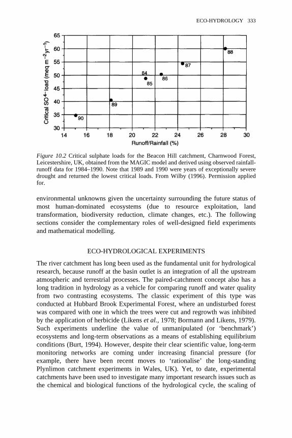
environmental unknowns given the uncertainty surrounding the future status ofmost human-dominated ecosystems (due to resource exploitation, landtransformation, biodiversity reduction, climate changes, etc.). The followingsections consider the complementary roles of well-designed field experimentsand mathematical modelling.
ECO-HYDROLOGICAL EXPERIMENTS
The river catchment has long been used as the fundamental unit for hydrologicalresearch, because runoff at the basin outlet is an integration of all the upstreamatmospheric and terrestrial processes. The paired-catchment concept also has along tradition in hydrology as a vehicle for comparing runoff and water qualityfrom two contrasting ecosystems. The classic experiment of this type wasconducted at Hubbard Brook Experimental Forest, where an undisturbed forestwas compared with one in which the trees were cut and regrowth was inhibitedby the application of herbicide (Likens et al., 1978; Bormann and Likens, 1979).Such experiments underline the value of unmanipulated (or ‘benchmark’)ecosystems and long-term observations as a means of establishing equilibriumconditions (Burt, 1994). However, despite their clear scientific value, long-termmonitoring networks are coming under increasing financial pressure (forexample, there have been recent moves to ‘rationalise’ the long-standingPlynlimon catchment experiments in Wales, UK). Yet, to date, experimentalcatchments have been used to investigate many important research issues such asthe chemical and biological functions of the hydrological cycle, the scaling of
Figure 10.2 Critical sulphate loads for the Beacon Hill catchment, Charnwood Forest,Leicestershire, UK, obtained from the MAGIC model and derived using observed rainfall-runoff data for 1984–1990. Note that 1989 and 1990 were years of exceptionally severedrought and returned the lowest critical loads. From Wilby (1996). Permission appliedfor.
ECO-HYDROLOGY 333
dynamic ecosystem behaviour, land surface-atmosphere interactions, and thehydrological effects of human activity (Farrell, 1995).
Ecologists have also been conducting controlled laboratory and fieldmanipulations since the 1960s in the style of ‘hard science’ (which somecommentators have unfairly attributed to ‘physics envy’). Laboratory systemshave many advantages, such as the replicability of experiments and the controlof a limited number of parameters. For example, closed chambers have beenused to investigate the specific issue of the sequestration of carbon by theterrestrial biosphere in response to rising concentrations of atmospheric CO2(Hungate et al., 1997). Again, there has been a strong argument for carefulexperimental design and the augmentation of laboratory results with long periodsof field observation—what some researchers refer to as ‘muddy boots biology’.However, it has been argued that too many ecological experimenters reducenature to oversimplified caricatures of the real world in their quest for cause andeffect (Roush, 1995). The remedy for such reductionism is to embrace morecomplexity and multiple causality in experimental designs, and to set up multipleworking hypotheses that can be subjected to unambiguous statistical testing.There has also been a call for a broadening of the spatial scales of ecologicalexperiments, because many natural processes such as mobility, dispersal andspecies interaction can only be observed from a macro-perspective (ibid.).
Controlled environment facilities, whether in the laboratory or the field, arehalfway houses between the simplicity and abstraction of mathematical modelsand the full complexity of the environment (Lawton, 1995). Here hydrologistsand ecologists have found common ground through experimental manipulationsof entire lake, catchment, terrestrial and marine ecosystems. One of the mostprominent of such experiments was the RAIN (Reversing Acidification InNorway) study of the effects of acid deposition on soil and river water quality(Wright et al., 1988). At Risdalsheia, Norway, acid rain was excluded from thewhole catchment by means of a roof, whereas at Sogndal the acid load wasartificially increased. The respective experiments demonstrated that aciddeposition effects are reversible, and that the onset of surface water acidificationcan occur after only a few years of acid deposition. The scientific principlesunderpinning whole-catchment experiments have subsequently been applied tostudies of liming and other measures to mitigate acidification (Warfvinge andSverdrup, 1988), to the manipulation of forest nutrient balances (Tietema et al.,1997), and to studies of the effects of elevated CO2 concentrations and temperatureon catchments (Schindler and Bayley, 1993). Manipulation experiments havealso been used to study nutrient enrichment, biogeochemical cycling and foodwebs in lake, ocean and terrestrial ecosystems (see Carpenter et al., 1995).
A significant feature of the most recent experiments has been the increasinglevel of international coordination and cooperation. This enables the repetition ofimportant experiments and the rationalisation of effort, as well as checks on thegenerality of results. For example, the Boreal Ecosystem-Atmosphere Study(BOREAS) was a large-scale international investigation that focused on
334 THE FUTURE OF ECO-HYDROLOGY
improving understanding of the exchanges of radiative energy, sensible heat,water, CO2 and other radiatively active trace gases between the boreal forest andthe lower atmosphere (Sellers et al., 1997). The field campaign was conductedbetween 1993 and 1997 and adopted a nested multi-scale measurement strategy(Figure 10.3) to integrate observations and process models over five scalesranging from the process study site (1 m2 to 100 m2) up to the region (1,000,000km2). The measurement and modelling activities were undertaken by eighty-fivescientific teams organised into six disciplinary groups (airborne fluxes andmeteorology, tower fluxes, terrestrial ecology, trace gas biogeochemistry,hydrology, and remote-sensing science). An important outcome of suchexperiments is the development of common data sets for model development andinter-comparison, as in the case of the Project for Intercomparison of Land-Surface Parameterization Schemes (PILPS) (Chen et al., 1997) or the Vegetation/Ecosystem Modeling and Analysis Project (VEMAP) (VEMAP members, 1995).However, the value of ‘big science’ field and/or model data sets is trulymaximised when the results are made freely available to the wider scientificcommunity. In this respect, the Climate Impacts LINK Project (Viner and Hulme,1997) has been an outstanding success. By the free dissemination of results fromthe UK Meteorological Office Hadley Centre climate change experiments, the‘impacts community’ has been able to conduct investigations using state-of-the-art climate scenarios, while returning important information concerning the
Figure 10.3 Multi-scale measurement strategy used in BOREAS (after Sellers et al.,1997). Permission applied for.
ECO-HYDROLOGY 335
climate model’s realism. For more details about the project, interested readersshould refer to the world wide web site: http://www.cru.uea.ac. uk/link.
Large-scale ecosystem experiments are also vital for the validation of existingmathematical models (Oreskes et al., 1994). A good example of an integratedfield manipulation and modelling experiment involved the evaluation of MAGIC(Model of Acidification of Groundwater In Catchments) (Wright et al., 1990).This model has a well-documented pedigree and has been widely used to studysoil and river water acidification in North America, Europe and Scandinavia. Themost recent field results suggest that MAGIC does not adequately simulateobserved inter-annual variations in water quality (Figure 10.4). This wasattributed to the lumped structure of the hydrological sub-model and poorrepresentations of aluminium dynamics (Cosby et al., 1995). Nonetheless, theseshortfalls provide a valuable focus for both future field experimentation and modelrefinement. However, such integrated experimentation presupposes the existenceof dedicated field sites, with sustained funding, in a diversity of habitats. Theimportance of such work should not be understated given that ecosystemexperiments are the most direct means of relating cause(s) and effect(s) at theactual scale of many environmental impacts (Carpenter et al., 1995).
PLANETARY SCALE ECO-HYDROLOGY
As has been shown, integrated field and modelling experiments affordconsiderable opportunities for theory building and model testing. However, lakewatershed experiments deal essentially with point to catchment-scale processes,have relatively limited sampling capabilities, and often involve the broad-scaleextrapolation of laboratory or field measurements to studies of global change.Clearly, there are many eco-hydrological problems that are beyond the scope ofconventional field monitoring systems. Thus, studies of landscape- to regional-,or regional to global-scale plant-water relations have largely depended upon, andbenefited enormously from, remote-sensing research. As Table 10.1 suggests,there have been considerable advances in the capabilities of remote-sensingplatforms to map hydrologically and ecologically relevant surface variables atregional scales and beyond. For example, Moulin et al. (1997) used NOAA/AVHRR satellite measurements to assess phenological stages of canopydevelopment at the global scale. Rhythms in vegetation succession exert a strongcontrol over seasonal energy and water exchanges between the Earth’s surfaceand the atmosphere. Similarly, Hall et al. (1995) used microwave data tomeasure soil moisture quantitatively under a variety of topographic andvegetation cover conditions. Such measurements have formed the basis of muchinteresting research into biogeochemical cycles, and hydrological and land-surface changes.
For example, Asner et al. (1998) suggest that at the ecosystem to biome scales(1 m−1 km resolution), remote sensing can provide valuable information on thestructural and biophysical attributes of individual
336 THE FUTURE OF ECO-HYDROLOGY
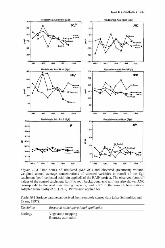
Table 10.1 Surface parameters derived from remotely sensed data (after Schmullius andEvans, 1997).
Discipline Research topic/operational application
Ecology Vegetation mappingBiomass estimation
Figure 10.4 Time series of simulated (MAGIC) and observed (treatment) volume-weighted annual average concentrations of selected variables in runoff of the Egilcatchment (roof, collected acid rain applied) of the RAIN project. The observed (control)values of the control catchment Rolf (no roof, background acid rain) are also shown. ANCcorresponds to the acid neutralising capacity, and SBC to the sum of base cations.Adapted from Cosby et al. (1995). Permission applied for.
ECO-HYDROLOGY 337
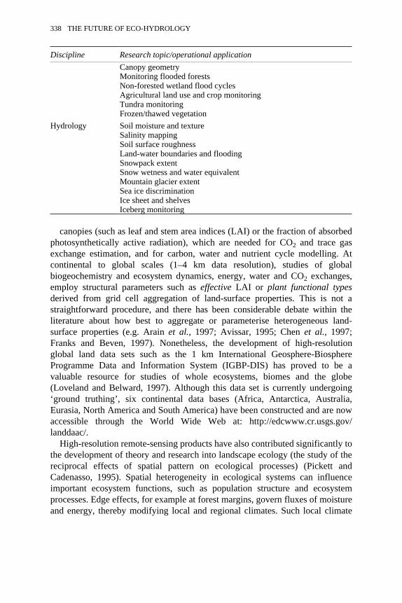
Discipline Research topic/operational applicationCanopy geometryMonitoring flooded forestsNon-forested wetland flood cyclesAgricultural land use and crop monitoringTundra monitoringFrozen/thawed vegetation
Hydrology Soil moisture and textureSalinity mappingSoil surface roughnessLand-water boundaries and floodingSnowpack extentSnow wetness and water equivalentMountain glacier extentSea ice discriminationIce sheet and shelvesIceberg monitoring
canopies (such as leaf and stem area indices (LAI) or the fraction of absorbedphotosynthetically active radiation), which are needed for CO2 and trace gasexchange estimation, and for carbon, water and nutrient cycle modelling. Atcontinental to global scales (1–4 km data resolution), studies of globalbiogeochemistry and ecosystem dynamics, energy, water and CO2 exchanges,employ structural parameters such as effective LAI or plant functional typesderived from grid cell aggregation of land-surface properties. This is not astraightforward procedure, and there has been considerable debate within theliterature about how best to aggregate or parameterise heterogeneous land-surface properties (e.g. Arain et al., 1997; Avissar, 1995; Chen et al., 1997;Franks and Beven, 1997). Nonetheless, the development of high-resolutionglobal land data sets such as the 1 km International Geosphere-BiosphereProgramme Data and Information System (IGBP-DIS) has proved to be avaluable resource for studies of whole ecosystems, biomes and the globe(Loveland and Belward, 1997). Although this data set is currently undergoing‘ground truthing’, six continental data bases (Africa, Antarctica, Australia,Eurasia, North America and South America) have been constructed and are nowaccessible through the World Wide Web at: http://edcwww.cr.usgs.gov/landdaac/.
High-resolution remote-sensing products have also contributed significantly tothe development of theory and research into landscape ecology (the study of thereciprocal effects of spatial pattern on ecological processes) (Pickett andCadenasso, 1995). Spatial heterogeneity in ecological systems can influenceimportant ecosystem functions, such as population structure and ecosystemprocesses. Edge effects, for example at forest margins, govern fluxes of moistureand energy, thereby modifying local and regional climates. Such local climate
338 THE FUTURE OF ECO-HYDROLOGY
change may be one of the environmental consequences of the piecemealdevelopment of the National Forest in the East Midlands, UK (Wilby, in press).
Continental-scale land-surface changes detected by Earth ObservationSystems (EOS) may have profound effects on regional hydrological andbiogeochemical processes (see, for example, the summaries in Pitman et al.,1993, or Wilby, 1995). The most popular modelling experiments are those toreplace tropical forests with pastures (e.g. Henderson-Sellers et al., 1993), or toreplace vegetation with desert (e.g. Xue and Shukla, 1993). This is typicallyaccomplished within general circulation models (GCMs) by altering the surfacealbedo and roughness, or gross soil properties, and then comparing the resultswith a control simulation. Most GCMs treat the hydrological cycle in terms of asingle, or overlying set of soil ‘buckets’; relatively few incorporate lateral waterexchanges, groundwater or climatically responsive surface vegetation (Miller etal., 1994; Polcher and Laval, 1994). For example, Lean and Rowntree (1997)found that the complete removal of the Amazonian forest would produce areamean decreases in evaporation of 0.76 mm day−1 (18 percent) and rainfall of 0.27mm day−1 (4 percent) and a rise in surface temperature of 2.3 °C. The rainfallchanges were attributed to increased albedo, resulting in reduced atmosphericmoisture convergence and ascent, while changes in both rainfall and evaporationwere found to be very sensitive to one soil parameter—the maximum infiltrationrate. On the other hand, Bonan (1997) asserts that the replacement of the naturalforests and grasslands of the United States has contributed to summer cooling,especially in the east, which has actually offset any warming due to greenhouseforcing.
Changes in the function and structure of terrestrial ecosystems may alsoinfluence the climate by means of biogeochemical feedbacks that regulate land-atmosphere exchanges of radiatively active gases such as carbon dioxide,methane and nitrous oxide, as well as exchanges of energy and water vapour(Melillo et al., 1996). Estimating the magnitude of the terrestrial carbon sink ishighly problematic, because the rate of carbon sequestration is a function of CO2and nitrogen fertilisation effects, changes in the area of agricultural land, the agestructure of biomes, species composition, ecosystem metabolism, susceptibilityto pathogens, and limiting factors such as drought or the frequency of fire.Terrestrial ecosystems are also significant sources of methane and nitrous oxide,the production of which is highly sensitive to soil moisture, temperature andoxygen levels. Similarly, as biomes shift in response to global warming, therewill be latitudinal changes in surface characteristics such as albedo, rooting depthand surface roughness, which in turn govern surface energy and water fluxes.Furthermore, physiological adjustments such as increasing stomatal resistance inthe presence of higher atmospheric CO2 concentrations, without changes in leafarea, could lead to increased soil moisture storage and additional surfacewarming over the land (Martin et al., 1989). However, some have argued that atthe planetary scale, land-surface changes are of less significance to the climatethan the thermal regime of the oceans and the spatial distribution of snow and ice
ECO-HYDROLOGY 339
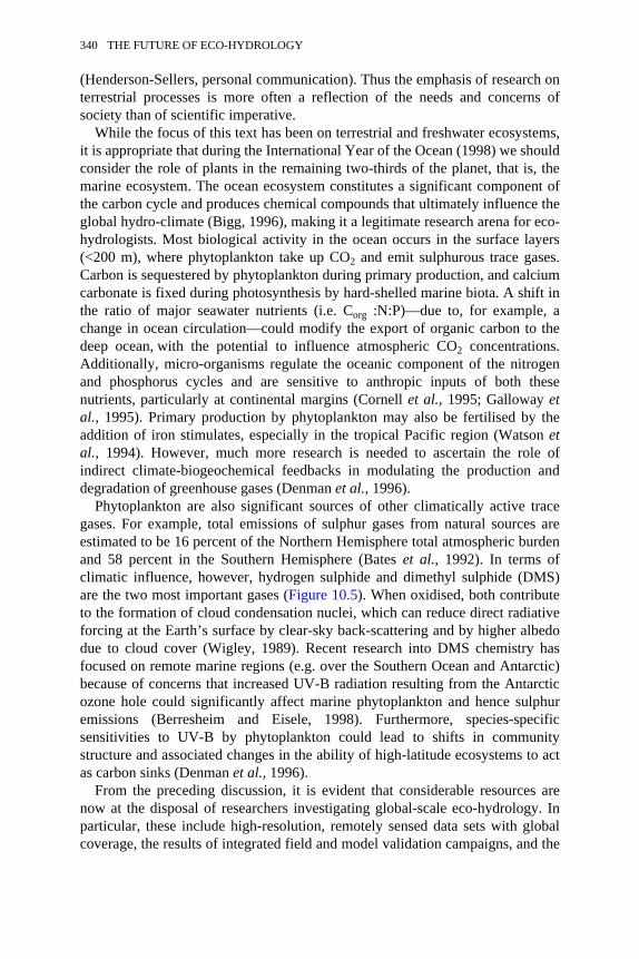
(Henderson-Sellers, personal communication). Thus the emphasis of research onterrestrial processes is more often a reflection of the needs and concerns ofsociety than of scientific imperative.
While the focus of this text has been on terrestrial and freshwater ecosystems,it is appropriate that during the International Year of the Ocean (1998) we shouldconsider the role of plants in the remaining two-thirds of the planet, that is, themarine ecosystem. The ocean ecosystem constitutes a significant component ofthe carbon cycle and produces chemical compounds that ultimately influence theglobal hydro-climate (Bigg, 1996), making it a legitimate research arena for eco-hydrologists. Most biological activity in the ocean occurs in the surface layers(<200 m), where phytoplankton take up CO2 and emit sulphurous trace gases.Carbon is sequestered by phytoplankton during primary production, and calciumcarbonate is fixed during photosynthesis by hard-shelled marine biota. A shift inthe ratio of major seawater nutrients (i.e. Corg :N:P)—due to, for example, achange in ocean circulation—could modify the export of organic carbon to thedeep ocean, with the potential to influence atmospheric CO2 concentrations.Additionally, micro-organisms regulate the oceanic component of the nitrogenand phosphorus cycles and are sensitive to anthropic inputs of both thesenutrients, particularly at continental margins (Cornell et al., 1995; Galloway etal., 1995). Primary production by phytoplankton may also be fertilised by theaddition of iron stimulates, especially in the tropical Pacific region (Watson etal., 1994). However, much more research is needed to ascertain the role ofindirect climate-biogeochemical feedbacks in modulating the production anddegradation of greenhouse gases (Denman et al., 1996).
Phytoplankton are also significant sources of other climatically active tracegases. For example, total emissions of sulphur gases from natural sources areestimated to be 16 percent of the Northern Hemisphere total atmospheric burdenand 58 percent in the Southern Hemisphere (Bates et al., 1992). In terms ofclimatic influence, however, hydrogen sulphide and dimethyl sulphide (DMS)are the two most important gases (Figure 10.5). When oxidised, both contributeto the formation of cloud condensation nuclei, which can reduce direct radiativeforcing at the Earth’s surface by clear-sky back-scattering and by higher albedodue to cloud cover (Wigley, 1989). Recent research into DMS chemistry hasfocused on remote marine regions (e.g. over the Southern Ocean and Antarctic)because of concerns that increased UV-B radiation resulting from the Antarcticozone hole could significantly affect marine phytoplankton and hence sulphuremissions (Berresheim and Eisele, 1998). Furthermore, species-specificsensitivities to UV-B by phytoplankton could lead to shifts in communitystructure and associated changes in the ability of high-latitude ecosystems to actas carbon sinks (Denman et al., 1996).
From the preceding discussion, it is evident that considerable resources arenow at the disposal of researchers investigating global-scale eco-hydrology. Inparticular, these include high-resolution, remotely sensed data sets with globalcoverage, the results of integrated field and model validation campaigns, and the
340 THE FUTURE OF ECO-HYDROLOGY
products of coupled land-atmosphere-ocean GCMs. Returning to the originalquotation, the final question is now raised as to how such eco-hydrologicalinformation might be applied.
APPLIED ECO-HYDROLOGY
The significance of plants to human well-being has long been recognised, as aSouth American tribal legend testifies: ‘the tropical rainforest supports the sky;cut down the trees and disaster follows’ (cited in Park, 1992). And yet thedegradation of the Earth’s terrestrial vegetated surface by human activities isoccurring at unprecedented levels. Daily (1995) estimated that the total areaaffected by soil, dryland and tropical moist forest degradation is 5.0 billionhectares, or 43 percent of the Earth’s vegetated surface (Figure 10.6). Despitethis shocking statistic, there has been a growing belief among environmentalscientists that a deeper understanding of the functioning and significance of eco-hydrological relations can result in the restoration or rehabilitation of degradedterrestrial ecosystems. In other words, eco-hydrological science can be applied ina positive way to protect or enhance landscapes, rather than negatively to exploitthem still further (Petts, 1990). This optimism is reflected in the publication oftexts such as The Ecological Basis for River Management (Harper and Ferguson,1995), Restoration of Aquatic Ecosystems (National Research Council, 1992) andThe Rivers Handbook: Hydrological and Ecological Principles (Calow and Petts,1992). The belief that environmental damage is reversible may also have intense
Figure 10.5 The marine biogeochemical cycle of DMS (dimethyl sulphide): production ofDMSP (dimethyl sulphonioproprionate) by phytoplankton; transformation by bacteria toDMS and by bacteria or photo-oxidation to DMSO (dimethyl sulphoxide); and alternativeutilisation pathways that may influence the quantity of DMS lost to the atmosphere (fromMalin et al., 1992). Permission applied for.
ECO-HYDROLOGY 341
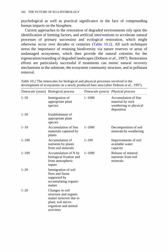
psychological as well as practical significance in the face of compoundinghuman impacts on the biosphere.
Current approaches to the restoration of degraded environments rely upon theidentification of limiting factors, and artificial interventions to accelerate naturalprocesses of primary succession and ecological restoration, which mightotherwise occur over decades or centuries (Table 10.2). All such techniquesstress the importance of retaining biodiversity via nature reserves or areas ofundamaged ecosystems, which then provide the natural colonists for theregeneration/reseeding of degraded landscapes (Dobson et al., 1997). Restorationefforts are particularly successful if treatments can mimic natural recoverymechanisms in the substrate, the ecosystem community structure, and in pollutantremoval.
Table 10.2 The timescales for biological and physical processes involved in thedevelopment of ecosystems on a newly produced bare area (after Dobson et al., 1997).
Timescale (years) Biological process Timescale (years) Physical process
1–50 Immigration ofappropriate plantspecies
1–1000 Accumulation of finematerial by rockweathering or physicaldeposition
1–50 Establishment ofappropriate plantspecies
1–10 Accumulation of finematerials captured byplants
1–1000 Decomposition of soilminerals by weathering
1–100 Accumulation ofnutrients by plantsfrom soil minerals
1–100 Improvements of soilavailable watercapacity
1–100 Accumulation of N bybiological fixation andfrom atmosphericinputs
1–1000 Release of mineralnutrients from soilminerals
1–20 Immigration of soilflora and faunasupported byaccumulating organicmatter
1–20 Changes in soilstructure and organicmatter turnover due toplant, soil micro-organism and animalactivities
342 THE FUTURE OF ECO-HYDROLOGY
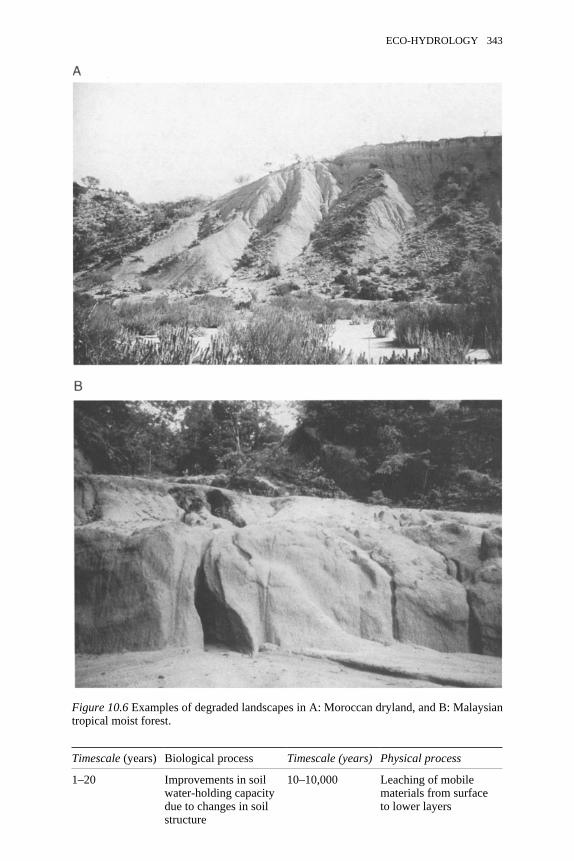
Timescale (years) Biological process Timescale (years) Physical process
1–20 Improvements in soilwater-holding capacitydue to changes in soilstructure
10–10,000 Leaching of mobilematerials from surfaceto lower layers
Figure 10.6 Examples of degraded landscapes in A: Moroccan dryland, and B: Malaysiantropical moist forest.
ECO-HYDROLOGY 343
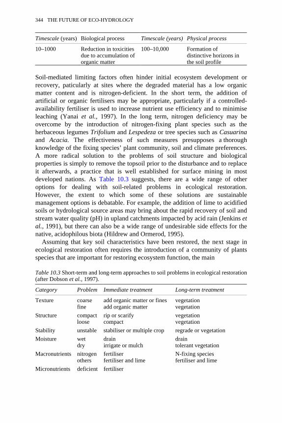
Timescale (years) Biological process Timescale (years) Physical process
10–1000 Reduction in toxicitiesdue to accumulation oforganic matter
100–10,000 Formation ofdistinctive horizons inthe soil profile
Soil-mediated limiting factors often hinder initial ecosystem development orrecovery, paticularly at sites where the degraded material has a low organicmatter content and is nitrogen-deficient. In the short term, the addition ofartificial or organic fertilisers may be appropriate, particularly if a controlled-availability fertiliser is used to increase nutrient use efficiency and to minimiseleaching (Yanai et al., 1997). In the long term, nitrogen deficiency may beovercome by the introduction of nitrogen-fixing plant species such as theherbaceous legumes Trifolium and Lespedeza or tree species such as Casuarinaand Acacia. The effectiveness of such measures presupposes a thoroughknowledge of the fixing species’ plant community, soil and climate preferences.A more radical solution to the problems of soil structure and biologicalproperties is simply to remove the topsoil prior to the disturbance and to replaceit afterwards, a practice that is well established for surface mining in mostdeveloped nations. As Table 10.3 suggests, there are a wide range of otheroptions for dealing with soil-related problems in ecological restoration.However, the extent to which some of these solutions are sustainablemanagement options is debatable. For example, the addition of lime to acidifiedsoils or hydrological source areas may bring about the rapid recovery of soil andstream water quality (pH) in upland catchments impacted by acid rain (Jenkins etal., 1991), but there can also be a wide range of undesirable side effects for thenative, acidophilous biota (Hildrew and Ormerod, 1995).
Assuming that key soil characteristics have been restored, the next stage inecological restoration often requires the introduction of a community of plantsspecies that are important for restoring ecosystem function, the main
Table 10.3 Short-term and long-term approaches to soil problems in ecological restoration(after Dobson et al., 1997).
Category Problem Immediate treatment Long-term treatment
Texture coarsefine
add organic matter or finesadd organic matter
vegetationvegetation
Structure compactloose
rip or scarifycompact
vegetationvegetation
Stability unstable stabiliser or multiple crop regrade or vegetationMoisture wet
drydrainirrigate or mulch
draintolerant vegetation
Macronutrients nitrogenothers
fertiliserfertiliser and lime
N-fixing speciesfertiliser and lime
Micronutrients deficient fertiliser
344 THE FUTURE OF ECO-HYDROLOGY

Category Problem Immediate treatment Long-term treatment
Toxicity low lime lime or tolerant speciespH high pyritic waste or organic
matterweathering
Heavy metals high organic matter or tolerantplants
inert covering orbioremediation
Organics high inert covering microbial breakdownSalinity high weathering or irrigate weathering or tolerant
species
component of the final ecosystem, or an element in the final biodiversity of theecosystem (Dobson et al., 1997). Insights into the ‘rules’ for assembling suchcommunities and natural rates of recolonisation have often come from studies ofchemical waste heaps or from violent volcanic eruptions such as those of MountSt Helens and Krakatau (Plage and Plage, 1985). However, it is unclear whetherefforts should be directed towards ecosystem restoration (of all that waspreviously present) or towards replacement (by a new but functionallyequivalent system). What is clear is that the ecological engineering should beundertaken at the landscape scale in order that natural immigration and dispersalmechanisms may be incorporated. For example, Noble and Dirzo (1997) suggestthat in forests used for logging, whole-landscape management is essential toensure that areas of intensive use are interspersed with areas of conservation andriver catchment protection.
There is considerable scope for the manipulation of eco-hydrologicalprocesses for the purpose of phyto-volatilisation, phyto-stabilisation or phyto-extraction of soils and groundwaters contaminated by heavy metals and certainorganic compounds. Phyto-extraction involves the use of plants to take up toxicmetals such as Zn, Ni, Cd, Pb, Cu and Co. For example, Robb and Robinson(1995) proposed the use of natural marshlands within former mining districts as asink for heavy metals. The biomass is then harvested and, in some cases, metalsmay be commercially recovered from incineration products. Examples of plantsendemic to metalliferous soils include Alyssum (Ni and Cr), Thlaspi (Zn, Cd andPb), and Brassica (Pb). Phyto-extraction can also be used to remove excessnutrients such as in nitrogen uptake via riparian buffer zones of poplar (Haycocket al., 1993) or through the judicious planting and management of new forests(Wilby, 1998). However, the efficiency of all such techniques is ultimatelygoverned by rates of plant growth relative to biomass and the bio-availability (bothchemically and hydrologically) of the contaminant. Furthermore, where thephyto-extraction involves the planting of large stands it is important that secondaryconflicts do not occur, for example with flood control or water resourcemanagement (Large et al., 1993).
The latter point underlines the necessity of undertaking eco-hydrologicalmanipulations within a holistic environmental framework that embraces both
ECO-HYDROLOGY 345
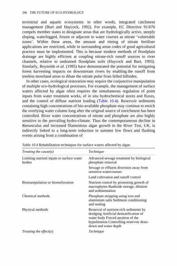
terrestrial and aquatic ecosystems: in other words, integrated catchmentmanagement (Burt and Haycock, 1992). For example, EC Directive 91/676compels member states to designate areas that are hydrologically active, steeplysloping, waterlogged, frozen or adjacent to water courses as nitrate ‘vulnerablezones’. Within these areas, the amount and timing of nitrate fertiliserapplications are restricted, while in surrounding areas codes of good agriculturalpractice must be implemented. This is because modern methods of floodplaindrainage are highly efficient at coupling nitrate-rich runoff sources to riverchannels, relative to undrained floodplain soils (Haycock and Burt, 1993).Similarly, Reynolds et al. (1995) have demonstrated the potential for mitigatingforest harvesting impacts on downstream rivers by enabling the runoff fromtreeless moorland areas to dilute the nitrate pulse from felled hillsides.
In other cases, ecological restoration may require the conjunctive manipulationof multiple eco-hydrological processes. For example, the management of surfacewaters affected by algae often requires the simultaneous regulation of pointinputs from water treatment works, of in situ hydrochemical stores and fluxes,and the control of diffuse nutrient loading (Table 10.4). Reservoir sedimentscontaining high concentrations of bio-available phosphate may continue to enrichthe overlying water column long after the original source of enrichment has beencontrolled. River water concentrations of nitrate and phosphate are also highlysensitive to the prevailing hydro-climate. Thus the contemporaneous decline inRanunculus and increased filamentous algae growth in the River Test, UK, isindirectly linked to a long-term reduction in summer low flows and flushingevents arising from a combination of
Table 10.4 Rehabilitation techniques for surface waters affected by algae.
Treating the cause(s) Technique
Limiting nutrient inputs to surface waterbodies
Advanced sewage treatment by biologicalphosphate removalSewage or effluent diversion away fromsensitive watercoursesLand cultivation and runoff control
Biomanipulation or biomelioration Nutrient control by promoting growth ofmacrophytes Bankside storage, dilutionand sedimentation
Chemical methods Phosphate stripping using iron andaluminium salts Sediment conditioningand sealing
Physical methods Removal of nutrient-rich sediments bydredging Artificial destratification ofwater body Forced aeration of thehypolimnion Controlling reservoir draw-down and water depth
Treating the effect(s) Technique
346 THE FUTURE OF ECO-HYDROLOGY
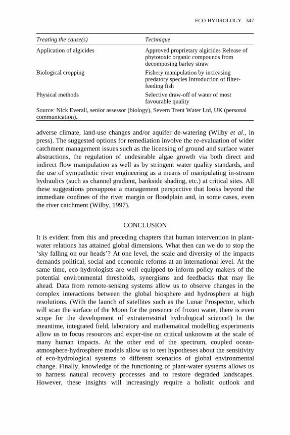
Treating the cause(s) Technique
Application of algicides Approved proprietary algicides Release ofphytotoxic organic compounds fromdecomposing barley straw
Biological cropping Fishery manipulation by increasingpredatory species Introduction of filter-feeding fish
Physical methods Selective draw-off of water of mostfavourable quality
Source: Nick Everall, senior assessor (biology), Severn Trent Water Ltd, UK (personalcommunication).
adverse climate, land-use changes and/or aquifer de-watering (Wilby et al., inpress). The suggested options for remediation involve the re-evaluation of widercatchment management issues such as the licensing of ground and surface waterabstractions, the regulation of undesirable algae growth via both direct andindirect flow manipulation as well as by stringent water quality standards, andthe use of sympathetic river engineering as a means of manipulating in-streamhydraulics (such as channel gradient, bankside shading, etc.) at critical sites. Allthese suggestions presuppose a management perspective that looks beyond theimmediate confines of the river margin or floodplain and, in some cases, eventhe river catchment (Wilby, 1997).
CONCLUSION
It is evident from this and preceding chapters that human intervention in plant-water relations has attained global dimensions. What then can we do to stop the‘sky falling on our heads’? At one level, the scale and diversity of the impactsdemands political, social and economic reforms at an international level. At thesame time, eco-hydrologists are well equipped to inform policy makers of thepotential environmental thresholds, synergisms and feedbacks that may lieahead. Data from remote-sensing systems allow us to observe changes in thecomplex interactions between the global biosphere and hydrosphere at highresolutions. (With the launch of satellites such as the Lunar Prospector, whichwill scan the surface of the Moon for the presence of frozen water, there is evenscope for the development of extraterrestrial hydrological science!) In themeantime, integrated field, laboratory and mathematical modelling experimentsallow us to focus resources and exper-tise on critical unknowns at the scale ofmany human impacts. At the other end of the spectrum, coupled ocean-atmosphere-hydrosphere models allow us to test hypotheses about the sensitivityof eco-hydrological systems to different scenarios of global environmentalchange. Finally, knowledge of the functioning of plant-water systems allows usto harness natural recovery processes and to restore degraded landscapes.However, these insights will increasingly require a holistic outlook and
ECO-HYDROLOGY 347
cooperation between scientists working in allied disciplines. Eco-hydrologyprovides a valuable example of the benefits that can accrue from such integration.
REFERENCES
Adkins, J.F., Boyle, E.A., Keigwin, L. and Cortijo, E. (1997) Variability of the NorthAtlantic thermohaline circulation during the last interglacial period, Nature 390:154–156.
Arain, A.M., Shuttleworth, W.J., Yang, Z.-L., Michaud, J. and Dolman, J. (1997)Mapping surface-cover parameters using aggregation rules and remotely sensedcover classes, Quarterly Journal of the Royal Meterorological Society 123:2325–2348.
Asner, G.P., Braswell, B.H., Schimel, D.S. and Wessman, C.A. (1998) Ecologicalresearch needs from multiangle remote sensing data. Remote Sensing of Environment63:155–165.
Avissar, R. (1995) Scaling of land-atmosphere interactions: an atmospheric modellingperspective, in Kalma, J.D. and Sivapalan, M. (eds) Scale Issues in HydrologicalModelling, Chichester: Wiley, pp. 435–452.
Bates, T.S., Lamb, B.K., Guenther, A., Dignon, J. and Stoiber, R.E. (1992) Sulfuremissions to the atmosphere from natural sources, Journal of Atmospheric Chemistry14:315–337.
Berresheim, H. and Eisele, F.L. (1998) Sulfur chemistry in the Antarctic TroposphereExperiment: an overview of project SCATE, Journal of Geophysical Research 103:1619–1627.
Bigg, G.R. (1996) The Oceans and Climate, Cambridge: Cambridge University Press.Blöschl, G. (1997) Preface to the special section on scale problems in hydrology, Water
Resources Research 33:2881.Bonan, G.B. (1997) Effects of land use on the climate of the United States, Climatic
Change 37:449–486.Bormann, F.H. and Likens, G.E. (1979) Pattern and Process in a Forested Ecosystem:
Disturbance, Development and the Steady State Based on the Hubbard BrookEcosystem Study, New York: Springer-Verlag, 253 pp.
Brussaard, L., Behan-Pelletier, V.M., Bignell, D.E., Brown, V.K., Didden, W., Folgarait,P., Fragoso, C., Freckman, D.W., Gupta, V.V.S.R., Hattori, T., Hawskworth, D.L.,Klopatek, C., Lavelle, P., Malloch, D.W., Rusek, J., Söderström, B., Tiedje, J.M. andVirginia, R.A. (1997) Biodiversity and ecosystem functioning in soil, Ambio 26:563–570.
Burt, T.P. (1994) Long-term study of the natural environment—perceptive science ormindless monitoring? Progress in Physical Geography 18:475–496.
Burt, T.P. and Haycock, N.E. (1992) Catchment planning and the nitrate issue: a UKperspective, Progress in Physical Geography 16:379–404.
Calow, P. and Petts, G.E. (eds) (1992) The Rivers Handbook: Hydrological andEcological Principles, Oxford: Blackwell Scientific Publications.
Carpenter, S.R., Chisholm, S.W., Krebs, C.J., Schindler, D.W. and Wright, R.F. (1995)Ecosystem experiments, Science 269:324–327.
348 THE FUTURE OF ECO-HYDROLOGY
Chapin III, F.S., Walker, B., Hobbs, R.J., Hooper, D.U., Lawton, J.H., Sala, O.E. andTilman, D. (1997) Biotic control over the functioning of ecosystems, Science 277:500–504.
Chen, T.H., Henderson-Sellers, A., Milly, P.C.D., Pitman, A.J., Beljaars, A.C.M., Polcher,J., Abramopoulos, F., Boone, A., Chang, S., Chen, F., Dai, Y., Desborough, C.E.,Dickinson, R.E., Dümenil, L., Ek, M., Garratt, J.R., Gedney, N., Gusev, Y.M., Kim,J., Koster, R., Kowalczyk, E.A., Laval, K., Lean, J., Lettenmaier, D., Liang, X.,Mahfouf, J.-F., Mengelkamp, H.-T., Mitchell, K., Nasanova, O.N., Noilhan, J.,Robock, A., Rosenzweig, C., Schaake, J., Schlosser,
C.A., Shulz, J.-P., Shao, Y., Shmakin, A.B., Verseghy, D.L., Wetzel, P., Wood, E.F.,Xue, Y., Yang, Z.-L. and Zeng, Q. (1997) Cabauw experimental results from theProject for Intercomparison of Land-Surface Parameterization Schemes, Journal ofClimate 10:1194–1215.
Cohen, J.E. (1995) Population growth and Earth’s human carrying capacity, Science 269:341–346.
Cornell, S., Rendell, A. and Jickells, T. (1995) Atmospheric inputs of dissolved organicnitrogen to the oceans, Nature 376:243–246.
Cosby, B.J., Wright, R.F. and Gjessing, E. (1995) An acidification model (MAGIC) withorganic acids evaluated using whole-catchment manipulations in Norway, Journal ofHydrology 170:101–122.
Daily, G.C. (1995) Restoring value to the world’s degraded lands, Science 269: 350–354.Denman, K., Hofmann, E. and Marchant, H. (1996) Marine biotic responses to
environmental change and feedbacks to climate, in Houghton, J.T., Meira Filho,L.G., Callander, B.A., Harris, N., Kattenberg, A. and Maskell, K. (eds) ClimateChange 1995: The Science of Climate Change. Contribution of Working Group I tothe Second Assessment Report of the Intergovernmental Panel on Climate Change,Chapter 10, Cambridge: Cambridge University Press.
Dhakhwa, G.B., Campbell, C.L., LeDuc, S.K. and Cooter, E.J. (1997) Maize growth:assessing the effects of global warming and CO2 fertilization with crop models,Agricultural and Forest Meteorology 87:253–272.
Dobson, A.P., Bradshaw, A.D. and Baker, A.J.M. (1997) Hopes for the future: restorationecology and conservation biology, Science 277:515–522.
Farrell, D.A. (1995) Experimental watersheds: a historical perspective, Journal of Soiland Water Conservation 50:432–437.
Franks, S.W. and Beven, K.J. (1997) Estimation of evapotranspiration at the landscapescale: a fuzzy disaggregation approach, Water Resources Research 33: 2929–2938.
Gallagher, R.B., Fischman, J. and Hines, P.J. (1995) Big questions for a small planet,Science 269:283.
Galloway, J.N., Schlesinger, W.H., Levy II, H., Michaels, A.F. and Schnoor, J.L. (1995)Nitrogen fixation: anthropogenic enhancement-environmental response. GlobalBiogeochemical Cycles 9:235–252.
Galy-Lacaux, C., Delmas, R., Jambert, C., Dumestre, J-F., Labroue, L., Richard, S. andGosse, P. (1997) Gaseous emissions and oxygen consumption in hydroelectric dams:a case study in French Guiana, Global Biogeochemical Cycles 11: 471–483.
Hall, F., Townsend, J. and Engman, T. (1995) Status of remote sensing algorithms forestimation of land surface state parameters, Remote Sensing of Environment 51:138–156.
ECO-HYDROLOGY 349
Harper, D.M. and Ferguson, A., (eds) (1995) The Ecological Basis for RiverManagement, Chichester: Wiley.
Haycock, N.E. and Burt, T.P. (1993) Role of floodplain sediments in reducing the nitrateconcentration of subsurface runoff: a case study in the Cotswolds, UK, HydrologicalProcesses 7:287–295.
Haycock, N.E., Pinay, G. and Walker, C. (1993) Nitrogen retention in river corridors:European perspective, Ambio 22:340–346.
Henderson-Sellers, A., Dickinson, R.E., Durbridge, T.B., Kennedy, P.J., McGuffie, K.and Pitman, A.J. (1993) Tropical deforestation: modelling local to regional-scaleclimate change, Journal of Geophysical Research 98:7289–7315.
Hildrew, A. and Omerod, S.J. (1995) Acidification, causes, consequences and solutions,in Harper, D.M. and Ferguson, A. (eds) The Ecological Basis for River Management,Chichester: Wiley.
Huettl, R.F. and Mueller-Dombois, D. (1993) Forest Decline in the Atlantic and PacificRegion, Berlin: Springer-Verlag.
Hungate, B.A., Holland, E.A., Jackson, R.B., Stuart-Chapin, F., Mooney, H.A. and Field,C.B. (1997) The fate of carbon in grasslands under carbon dioxide enrichment,Nature 388:576–579.
Hurrell, J.W. (1995) Decadal trends in the North Atlantic oscillation: regional temperatureand precipitation, Science 269:676–679.
James, L.D. (1991) Hydrology: infusing science into a demand-driven art, in Bowles,D.S. and O’Connell, P.E. (eds) Recent Advances in the Modelling of HydrologicSystems, the Netherlands: Kluwer Academic Publishers, pp. 31–43.
Jenkins, A., Waters, D. and Donald, A. (1991) An assessment of terrestrial limingstrategies in upland Wales, Journal of Hydrology 124:243–261.
Large, A.R.G., Petts, G.E., Wilby, R.L. and Greenwood, M.T. (1993) Restoration offloodplains: a UK perspective, European Water Pollution Control 3:44–53.
Lawton, J.H. (1995) Ecological experiments with model systems, Science 269: 328–331.Lean, J. and Rowntree, P.R. (1997) Understanding the sensitivity of a GCM simulation of
Amazonian deforestation to the specification of vegetation and soil characteristics,Journal of Climate 10:1216–1235.
Likens, G.E., Bormann, F.H., Pierce, R.S. and Reiness, W.A. (1978) Recovery of adeforested ecosystem, Science 199:492–496.
Loveland, T.R. and Belward, A.S. (1997) The IGBP-DIS global 1 km land cover data set,DISCover: first results, International Journal of Remote Sensing, 18:3289–3295.
Malin, G., Turner, S.M. and Liss, P.S. (1992) Sulfur: the plankton/climate connection,Journal of Phycology 28:590–597.
Manabe, S. and Stouffer, R.J. (1995) Simulation of abrupt climate change induced byfreshwater input to the North Atlantic Ocean, Nature 378:165–167.
Martin, P., Rosenberg, N.J. and McKenney, M.S. (1989) Sensitivity of evapotranspirationin a wheat field, a forest and a grassland to changes in climate and the direct effectsof carbon dioxide, Climatic Change 14:117–151.
McGrady-Steed, J., Harris, P.M. and Morin, P.J. (1997) Biodiversity regulates ecosystempredictability, Nature 390:162–165.
Melillo, J.M., Prentice, I.C., Farquhar, G.D., Schulze, E.-D. and Sala, O.E. (1996)Terrestrial biotic responses to environmental change and feedbacks to climate,in Houghton, J.T., Meira Filho, L.G., Callander, B.A., Harris, N., Kattenberg, A. andMaskell, K. (eds) Climate Change 1995: The Science of Climate Change.
350 THE FUTURE OF ECO-HYDROLOGY
Contribution of Working Group I to the Second Assessment Report of theIntergovernmental Panel on Climate Change, Chapter 9, Cambridge: CambridgeUniversity Press.
Miller, J.R., Russell, G.L. and Caliri, G. (1994) Continental scale river flow in climatemodels, Journal of Climate 7:914–928.
Moulin, S., Kergoat, L., Viovy, N. and Dedieu, G. (1997) Global-scale assessment ofvegetation phenology using NOAA/AVHRR satellite measurements, Journal ofClimate 10:1154–1170.
Myers, N. (1995) Environmental unknowns, Science 269:358–360.Naeem, S. and Li, S. (1997) Biodiversity enhances ecosystem reliability, Nature 390:
507–509.National Research Council (1992) Restoration of Aquatic Ecosystems, Washington:
National Academy Press.Noble, I.R. and Dirzo, R. (1997) Forests as human-dominated ecosystems, Science 277:
522–525.Oreskes, N., Shrader-Frechette, K. and Belitz, K. (1994) Verification, validation and
confirmation of numerical models in the earth sciences, Science 263: 641–646.Palmer, M., Covich, A.P., Finlay, B.J., Gibert, J., Hyde, K.D., Johnson, R.K., Kairesalo, T.,
Lake, S., Lovell, C.R., Naiman, R.J., Ricci, C., Sabater, F. and Strayer, D. (1997)Biodiversity and ecosystem processes in freshwater sediments, Ambio 26:571–577.
Park, C.C. (1992) Tropical Rainforests, London: Routledge.Petts, G.E. (1990) Water, engineering and landscape: development, protection and
restoration, in Cosgrove, D. and Petts, G.E. (eds) Water, Engineering and Landscape,London: Belhaven Press.
Pickett, S.T.A. and Cadenasso, M.L. (1995) Landscape ecology: spatial heterogeneity inecological systems, Science 269:331–334.
Pitman, A.J., Durbridge, T.B. and Henderson-Sellers, A. (1993) Assessing climate modelsensitivity to prescribed deforested landscapes, International Journal of Climatology13:877–898.
Plage, D. and Plage, M. (1985) Java’s wildlife returns, National Geographic 167:750–771.
Polcher, J. and Laval, K. (1994) The impact of African and Amazonian deforestation ontropical climate, Journal of Hydrology 155:389–405.
Reynolds, B., Stevens, P.A., Hughes, S., Parkinson, J.A. and Weatherby, N.S. (1995)Stream chemistry impacts of conifer harvesting in Welsh catchments, Water, Air andSoil Pollution 79:147–170.
Robb, G.A. and Robinson, J.D.F. (1995) Acid drainage from mines, Geographical Journal,161:47–54.
Rodhe, H., Charlson, R. and Crawford, E. (1997) Svante Arrhenius and the greenhouseeffect, Ambio 26:2–5.
Root, T.L. and Schneider, S.H. (1995) Ecology and climate: research strategies andimplications, Science 269:334–341.
Roush, W. (1995) When rigour meets reality, Science 269:313–315.Schindler, D.W. and Bayley, S.E. (1993) The biosphere as an increasing sink for
atmospheric carbon: estimates from increased nitrogen deposition, GlobalBiogeochemical Cycles 7:717–733.
Schmullius, C.C. and Evans, D.L. (1997) Synthetic aperture radar (SAR) frequency andpolarization requirements for applications in ecology, geology, hydrology, and
ECO-HYDROLOGY 351
oceanography: a tabular status quo after SIR-C/X-SAR, International Journal ofRemote Sensing 18:2713–2722.
Sellers. P.J., Hall, F.G., Kelly, R.D., Black, A., Baldocchi, D., Berry, J., Ryan, M.,Ranson, K.J., Crill, P.M., Lettenmaier, D.P., Margolis, H., Cihlar, J., Newcomer, J.,Fitzjarrald, D., Jarvis, P.G., Gower, S.T., Halliwell, D., Williams, D., Goodison, B.,Wickland, D.E. and Guertin, F.E. (1997) BOREAS in 1997: Experiment overview,scientific results and future directions, Journal of Geophysical Research 102:28731–28769.
Stocker, T.F. and Schmittner, A. (1997) Influence of CO2 emission rates on the stabilityof the thermohaline circulation, Nature 388:862–865.
Tietema, A., Beier, C., de Visser, P.H.B., Emmett, B.A., Gundersen, P., Kjønaas, O.J. andKoopmans, C.J. (1997) Nitrate leaching in coniferous forest ecosystems: theEuropean field-scale manipulation experiments NITREX (nitrogen saturationexperiments) and EXMAN (experimental manipulation of forest ecosystems),Global Biogeochemical Cycles 11:617–626.
Tilman, D. and Downing, J.A. (1994) Biodiversity and stability in grasslands. Nature367:363–365.
VEMAP members (1995) Vegetation/ecosystem modeling and analysis project:comparing biogeography and biogeochemistry models in a continental-scale study ofterrestrial ecosystem responses to climate change and CO2 doubling, GlobalBiogeochemical Cycles 9:407–437.
Viner, D. and Hulme, M. (1997) The Climate Impacts LINK Project: Applying Resultsfrom the Hadley Centre’s Climate Change Experiments for Climate Change ImpactsAssessments, Norwich: Department of the Environment, Transport and the RegionsClimatic Research Unit, 17 pp.
Vitousek, P.M., Mooney, H.A., Lubchenco, J. and Melillo, J.M. (1997) Humandomination of Earth’s ecosystem, Science 277:494–499.
Warfvinge, P. and Sverdrup, H. (1988) Soil liming as a measure to mitigate acid runoff,Water Resources Research 24:710–712.
Watson, A.J., Law, C.S., Van Scoy, K.A., Millero, F.J., Yao, W., Friederich, G.,Liddicoat, M.I., Wanninkhof, R.H., Barber, R.T. and Coale, K. (1994) Implicationsof the ‘Ironex’ iron fertilisation experiment for atmospheric carbon dioxideconcentrations, Nature 371:143–145.
Watson, R.T., Zinyowera, M.C., Moss, R.H. and Dokken, D.J. (eds) (1998) The RegionalImpacts of Climate Change: An Assessment of Vulnerability, a special report of IPCCWorking Group II, Cambridge: Cambridge University Press.
Wigley, T.M.L. (1989) Possible climate change due to SO2-derived cloud condensationnuclei, Nature 339:365–367.
Wigley, T.M.L., Richels, R. and Edmonds, J.A. (1996) Economic and environmentalchoices in the stabilization of atmospheric CO2 concentrations, Nature 379:240–243.
Wilby, R.L. (1995) Greenhouse hydrology, Progress in Physical Geography 19:351–369.
Wilby, R.L. (1996) Critical loads’ sensitivity to climate change, EnvironmentalConservation 22:363–365.
Wilby, R.L. (ed.) (1997) Contemporary Hydrology: Towards Holistic EnvironmentalScience, Chichester: Wiley, 354 pp.
352 THE FUTURE OF ECO-HYDROLOGY

Wilby, R.L. (in press) Hydrological impacts of the National Forest, special issue of EastMidlands Geographer.
Wilby, R.L., Cranston, L.E. and Darby, E.J. (in press) Factors governing macrophytestatus in Hampshire chalk streams: implications for catchment management, Journalof the Chartered Institute of Water and Environmental Management.
Worrall, J.J. (1994) Relationships of acid deposition and sulfur dioxide with forestdiseases, in Godbold, D.L. and Hüttermann, A. (eds) Effects of Acid Rain on ForestProcesses, Chichester: Wiley, Chapter 5.
Wright, R.F., Cosby, B.J., Flaten, M.B. and Ruess, J.O. (1990) Evaluation of anacidification model with data from manipulated catchments in Norway, Nature 343:53–55.
Wright, R.F., Lotse, E. and Semb, A. (1988) Reversibility of acidification shown bywhole-catchment experiments, Nature 334:670–675.
Xue, Y. and Shukla, J. (1993) The influence of land surface properties on Sahel climate.Part I: desertification, Journal of Climate 6:2232–2245.
Yanai, J., Nakano, A., Kyuma, K. and Kosaki, T. (1997) Application effects of controlled-availability fertilizer on dynamics of soil solution composition, Soil Science Societyof America Journal 61:1781–1786.
ECO-HYDROLOGY 353

INDEX
ABA (abscisic acid) 16Abies see firAbrahams, A.D. 96abscisic acid see ABAabsorption 19, 20–3, 283acceleration 13acid rain 160, 350, 353acidity 159acidophiles 157acrotelm 153–5, 156adaptation 103, 131, 134, 136, 211, 250;
biochemical 270;physiological 88, 270;structural 270;submergence 133, 251;survival and reproduction 237
Addiscott, T.M. 308adenosine triphosphate see ATPadhesion 62adiabatic effects 67aeolian activity 88aeration 132, 134, 154, 155;
poor 211aerenchyma 133, 134, 148aerobic conditions 35, 133, 208afforestation 81Africa:
East 103, 273;North 81, 89, 105;South 80, 87;sub-Saharan 89;West 189, 204;see also Egypt;Hoggar;Libya;Niger;
Sahara;Sahel;Senegal;Sudan
agriculture 50, 51;intensification 81;rain-fed and irrigated 81;small-scale 108agroforestry 189
air 26, 192;ambient 16, 18, 19;bubbles 27, 28;bulk 33;difference in temperature between leafand 29;dissolution of 28;heat capacity of 32;passage prevented 27;saturation deficit 191;solubility in water 28;turbulence 33;vapour pressure deficit 205;vertical convection 31;see also air humidity deficit
air humidity deficit:canopy conductance and 202;increase in 219, 222;stomatal behaviour and 199, 201, 215
Alaska 146albedo 40, 43, 48, 155;
changes 68;higher 82;modified 51
algae 88, 91, 243, 247, 270, 284;epiphytic 245, 252;filamentous 245, 366;
354

planktonic 271allelopathy 246, 255Allen, S.J. 193, 194, 223allochthonous solids/inputs 146, 269alluvial features:
aquifers 107, 247;deposition 129, 160
altitudes 102aluminium concentration 146Amazonian forest 90, 186, 189, 202, 205,
358;Ji-Paraná 203;Marabá 203
America see USAammonium 146amplitude fluctuations 140–2analytical methods/solutions 332, 334anatomical structures 133Andersen, F.O. 149Anderson, M.P. 307animals 204;
choice of food 91;small, burrows 208
ANN (artificial neural network)approaches 58
annuals 85, 87, 135;biseasonal 88;opportunistic 141
anoxia 131, 133, 134, 148, 161;avoidance of 136
Antarctic Ocean 360anthropic impact/effects 40, 65;
dryland plants 106–8;interference 349;responses to change 58
apoplastic water 26approximation:
Dupuit-Forchheimer 321, 325;exact 335;numerical 335
aquatic habitats 244;amphibious 238;backwater-pool 247;in-stream 238, 243;interstitial 251;macrophyte communities 245;micro- 243;river 237;
watery 127;wet, wetland species restricted to 137
aquifers:alluvial 107, 247;channel 238
Argentina 82;Patagonia 89
arid environments 27, 34, 78, 105aridification 81, 82aridity 87, 276;
extreme 88Arizona 85, 90;
Sycamore Creek 284;Walnut Gulch 86, 96, 97, 100
Armstrong, W. 131, 132–3, 134, 149Arrhenius, Svante 350ash forest 201, 207Asner, G.P. 357–8Atlantic Ocean 102;
North 58, 351atmosphere 16, 28, 60, 69, 131, 192;
above dry and wet surfaces 48;aerodynamic mixing with tree canopies207;connection severed 133;CO2 concentrations 57;cyclonicity 58;dry 223;gaseous escape to 277;humidity 185;simulating features 65, 69;spatial characteristics 67;vapour flux convergence 43;variables 82;water returns as transpiration 183;see also SPAC;SVATs
ATP (adenosine triphosphate) 11Aulehm deposits 95Australia 86, 87, 210;
central 79;eastern 89;Melbourne 54;New South Wales 193;Queensland 203, 209;south 80;southwest 80;Victoria 55;
INDEX 355

western 50autochthonous development 269, 284, 287auxiliary variables 62AVHRR (Advanced Very High Resolution
Radiometer) 43, 62, 357Avissar, R. 48AWS (automatic weather station) 84, 213,
218Azores 80
bacteria 270;cyano- 271
badlands (marl) 86BAHC (Biological Aspects of the
Hydrological Cycle) 58Bailey, W.G. 65Baird, A.J. 101, 314, 333, 337banks:
ditch 151–2;river/stream 94, 107, 143, 238, 246
Barbero, M. 108Bardossy, A. 58barley 147Barnes, H.H. 241base-richness 157, 158–60, 161basins 273, 275, 276, 281;
drainage 282, 284;morphology 284–8
Bathurst, J.C. 242, 313Beadle, C.L. 214Beckhoven, K. van 149Bedford, B.L. 149bedrock 242, 284beech forest 201, 207Bellamy, D.J. 146Beven, K.J. 42, 62–3, 310Bharucha, F.R. 142bicarbonate 146, 159, 255biodiversity 65, 244, 350biogeochemistry 197, 269biological processes 99, 246, 251, 254, 277;
lowland streams 245;potential of land 81;‘resetting’ 257;uptake 163;utilisation 284;
see also BAHC biomass 197, 242, 256,258, 350;above-ground 80;algal 284;dead 246;extant community 272;hill-slope 111;inverse relationship to velocity 241;organic, accumulation 283;photosynthetically active 43;seasonal maximum 255;woody, low 109
biophysical indicators 43biota 247, 257, 258, 269;
assemblage 65;emigrating 277;global 350;interactions 41, 152;lake distribution 275;life-cycles 245;marine, hard-shelled 359;photosynthetic 285;variables 138
Black, T.A. 201black box system 302, 307Blöschl, G. 39, 46, 48Blunder, M.A. 108Boatman, D.J. 132–3bogs 159, 160;
blanket 130;drought stress in 136;hill 130;ombrogenous 137, 150–1, 155;P-limited 161;raised 130, 151;topogenous 130
Bolivia 82Bonell, M. 203boreal region 129;
forest 197, 210BOREAS (Boreal Ecosystem-Atmosphere
Study) 197, 354‘bottom-up’ techniques 51Boucher, K. 42–3Bouldin, D.R. 149boundary conditions 60, 81, 87, 140, 221,
323;diffusion layers 246, 254;
356 INDEX
hydrochemical 162;lake 293;layer conductance 196;turbulent 192;uncertainty 274;see also channel boundaries
Boussinesq equation 321, 323, 325, 335,336
Bowen Ratio method 32, 185, 190–2, 213,324
bracken 201, 211, 215–16Brandt, C.J. 90Brazil 188, 204;
see also Amazonian forest;Manaus
Broadhurst, L.J. 242broadleaf forests/woodlands 182, 187, 188,
187, 197–8;temperate 187, 197–8, 210, 222;transpiration 211
Brooker, M.P. 242Bruijnzeel, L.A. 186, 188, 202, 203, 209Brutsaert, W.H. 275bryophytes 136, 149, 247budgets energy 29–33, 275, 276;
nitrogen 284;nutrient 207, 283
buffer strips 256Bugmann, H.K.M. 56Burch, G.J. 209burrows 208Burrows, D.A. 89Busch, D.E. 308bush 142, 204;
creosote 84–5, 86;holly oak 91;tar 85, 86;tiger 81, 204
caatinga vegetation 204Cabral, O.M.R. 218calcareous drift regions 274calcite 161calcium 163Calder, I.R. 185, 189, 193, 196Caldwell, M.M. 22, 210–11California:
chaparral species 27, 210;climate 92;Tulelake 103
canonical correlation technique 58canopies 87, 182, 199, 202, 214–15, 219;
aerodynamic mixing of atmospherewith 207;branches not angled upwards 208;broadleaf 187;broken 88;complex 196;conductance 33, 55, 196, 213;dry canopies, transpiration from 190;edges 205, 206;lower-level 90;need for access 196, 197;open 99;recruitment 57;resistance 43, 51;roots confined within 210;short-term evaporation from 185;size 86;sparse 96;structure of dryland plants 98;tropical forest 188;very dense 184;water storage on 189
capillary forces/properties 27, 143, 150carbohydrate reserves 134carbon 87, 152, 197, 353;
content in soils 206;depletion 246;global cycle 351;inorganic 255;organic 256;photosynthetic gain 243;sequestered 359
carbon dioxide 196, 351;atmospheric, doubled 68;diffusion of 16, 254, 255;dissolved 246;leaf internal concentration 205;measurement 192
Carex see sedgeCarpenter, S.R. 246catchment scales 40, 41, 44, 52, 54
catchments 68, 94, 208;chalk 257;
INDEX 357
coastal 92;forested 89, 184;grassland 209;paired 89, 90;position of stream within 240;small river 67;stormflow response of 209;topography 63
catenary process 23catotelm 153–4;
damaged 155Cauchy condition 323cavitation 27, 223;
xylem 34CCM (Community Climate Model) 65cells see plant cellscellulose walls 13Central Europe 151Cermák, J. 195chalk 211, 257channel boundaries 240, 241, 244;
flexible 242channel flow 240, 248–53;
resistance 241, 242–7channelisation 85channels 249;
beds 238, 240, 242, 247;morphology 237, 252;slope of 240;width of 240;see also channel boundaries;channel flow chaotic category 46
chaparral species 27, 210Chapin, F.S. 51Chapman, J.M. 151–2characteristic observation scales 41–4Charney, J.G. 204chemical composition:
stemflow 207, 208;water 157–64, 224
chemicals/chemical processes 207, 279;anaerobic 288;analyses 146;potential 12;transformations 131, 132
chemistry 206, 245, 309Cherry, J.A. 325Chezy’s semi-empirical equation 237
Chihuahan Desert 84Chile 79, 92chloroplasts 16Chopping, M. 65circulation:
global 79;mesoscale 48–9;see also GCMs
clay 193, 207, 216clearances/clearing 51, 95, 107;
‘slash and burn’ 209;small-scale 108
climate 32, 41, 55, 58, 202;cooler, wetter 130;dryland 79–80, 91, 94, 98;future conditions 60;global 51, 81, 359;impact of shifts on vegetation 94;low-rainfall 187;Mediterranean-type 92;medium- and long-term dynamics 81;morphological state of 33;natural heterogeneity of 65;role of forests in modifying 181;tropical 91;variability, eco-hydrological impact of108–12;variations in 45, 104–6;see also climate change;microclimate;palaeoclimate reconstructions climatechange 351, 358;dryland 94, 108–12;Earth’s orbital activity and 104;experiments 98;global 55;impacts 39, 60, 67;Mediterranean 95, 102;Pleistocene 104;predictions 188;simulating 69
Climate Impacts LINK Project 355climatology 57, 67, 204, 331clones 250clouds:
convective and precipitating 67–8;feedback effects 41;formation 82;
358 INDEX

orographic 65CO2 see carbon dioxideCoal Measures 52cohesion tension see C-T theoryco-kriging 46Collier, C.G. 46colonisation 129, 132, 147, 244, 287;
aggressive 249;invertebrate 245;littoral macrophytes 280;photosynthetic biota 285;rapid 258;river 243;stream 246
Colorado:Denver 60;State University 65
compaction 91, 108competition 109, 148, 244;
for light 56;for space 251;water table ranges and 158–9
competitive advantage 108composite images 51composition 140, 143, 146;
changes 137;chemical 157–64, 207, 208, 224;community 141, 256;controlled 142;floristic 146, 159;ionic 158, 159;substrate 257;variation in 147
concentrations 12, 28, 133, 159;aluminium 146;bicarbonate 146;carbon content in soils 206;CO2 16, 57, 68, 196, 205;dissolved salts 158;greenhouse gas 348–9;iron 147;leaf area 207;nitrogen 284;nutrient 160, 163, 292;osmolal 13;oxygen 278, 280;rainfall 186;reduced toxins 147;
sediment 94;solute 13, 147;sulphide 134;throughfall 206, 209;water vapour 32
condensation 276conductance:
aerodynamic 33, 191;axial 22, 23;boundary layer 196;bulk surface 191;canopy 33, 55, 196, 213;hydraulic 34;inverse 26;leaf 18, 55;radial 22, 23;surface 68, 196, 199, 205, 213, 218;whole-root 22;see also stomatal conductanceconductivity 27, 44;electrical 158, 159;hydraulic 23, 24, 47, 154, 155, 208–9;specific 24, 25
conduits 13, 26, 27, 208coniferous forests 102, 104, 211–16, 221–3;
rainfall interception 186, 187, 189;temperate 197–8, 210, 211–16, 221–3;transpiration 211
conservation 139;planning 65;problems 4
continuity principle 1controlled environment facilities 353convective activity:
air, vertical 31–2;clouds 67–8;rainfall 5
convergence (atmospheric vapour flux) 43;see also ITCZ
Conway, D. 58Conway, V.M. 134, 136cooling:
evaporative 19;global onset 102;Pleistocene 104
Cooper, J.D. 209coppice see SRCcovariance 40;
INDEX 359
eddy 185covariates 46, 62cracking 208Crampton, C.B. 205Crawford, R.M.M. 132credibility 318, 339crops 183, 189, 204, 223;
annual 50;monitoring 43;North African 81;short 193;simple 97;sparse 99;tree 107
cryptodysaptic structure 156crystallisation 158C-T (cohesion-tension) theory 13, 26–8Culf, A.D. 204culms 134cultura promiscua techniques 107currents 245, 251, 257, 279;
wave-induced 280cut-tree technique 193cycling 269, 277, 279Czarnowski, M.S. 186Czech Republic 252
D20 see deuterium oxideDaily, G.C. 361dams 247Darcy’s law 12, 24, 305, 306, 321, 325,
328, 337–9 passimDarcy-Richards equation 325, 327, 336Darcy-Richards-type flow 311data 60, 61, 103, 106, 187, 204;
atmospheric 65;AWS 213;digital 64;interrogation 44;logging requirements 196;lysimeter 193;oxygen isotope 102;pollen 104, 107;rainfall 189;satellite 46;sets 43, 65, 99, 152;software for manipulating 62;
sub-spatial 40Davis, C.B. 139Davis, F.W. 89Davis, Stephen 20Dawson, F.H. 242Dawson, T.E. 51DCA (detrended correspondence analysis)
308de Mars, H. 144–5Dead Sea 274debris:
organic 257–8;woody 247, 284
decomposers 258decomposition 145, 153, 159, 256, 270,
277;organic matter 286
DECORANA (computer program) 308defoliation 34deforestation 81, 107;
regional 40degradation 89, 254, 258, 361;
effects of climatic change on 95;land 82
dehydration 27denitrification 161, 256, 284density:
insect larvae 245;leaf 91, 211, 216;root 149;snow and ice 275–6;soil 210;stem 150, 216;vegetation 243;water 13, 22, 45;see also flux density
denudation 91deposition 238, 354;
acidic, critical loads 352;alluvial 129, 160;dry 207
deposits 251;completion 280;diplotelmic 154
Derbyshire Peak District 51desertification 95, 204;
experiments 82deserts 103;
360 INDEX
coastal 79;dry, hot 79;extreme 87;true 87;see also EFEDA;steppe
desiccation 136desorption processes 161detoxification 134detritivores 258detritus:
autochthonous 284;macrophyte 246, 270;particulate 246, 270, 271, 280
deuterium oxide 196developing countries 189dew 79, 99diaspores 249Diaz Fiernos, F. 98dicots 315die-back 94, 95Dietrich, W.E. 203diffusion:
boundary layer thinning 246;carbon dioxide 16, 254, 255;Fick’s law 18;gaseous 134;nutrient 270;overland flow 97;oxygen 35, 131, 133, 254, 255;phosphate and ammonium 146;turbulent 192
digital elevations 62, 64digital terrain models see DTMsdimensional analysis 57Dingman, S.L. 240, 314, 338Dirichlet condition 232discharge 51, 279;
continuity of 242;estimating 241;grassland catchment 209;groundwater 130, 157, 163
discontinuity 46, 56, 350, 351disequilibria 140;
quasi-cyclical 57disorganised/organised variability 49–50dispersal 57, 135, 249, 250dissipation:
energy 244, 247, 273;thermal 195–6;water excess 155
dissolved substance transport 246distance:
change of energy with 12;water transport 96distribution 156, 157, 163, 243, 257;biogeographic 65;biota, lake 275;carbon 206;closely related species 148;cyclonic mean wet day 58;influenced 151;macrophyte 244;microtopographical 150;natural vegetation 65;nutrients in lakes 277–84;patchy 244;phytotoxins and 147;probability 58, 59, 310;regulating 140;rooting 57, 210;seed 144;shoreline 148;soil moisture 209–10;soil water 55;spatial 55, 60, 62, 65, 98, 209;techniques 61–6;understanding 247;vegetation, principal factors governing51–2;vertical 216;wetland species 136–45 passim
disturbance 148, 244, 250, 252, 257;cycles 108;due to flooding 56;frequent 135, 258;vulnerability to 106
ditch banks 151–2diversity 88, 141, 350;
see also biodiversityDixon, H.H. 26DMS (dimethyl sulphide) 360dog’s mercury 201, 207Dooge, J.C.I. 41Douglas, I. 91Downing, J.A. 350
INDEX 361

downscaling techniques 40, 67;statistical 58–61
drag forces 242drainage 137, 138, 139, 190, 282, 284;
downslope 63;field 52;floodplain 365;impeded 128, 130;lake basin 273;measured 193;meteoric water 130;minimising 207;network 44;zero 193
drought 19, 67, 89, 111, 136, 204, 215,256–8;
effects on fluvial hydrosystems 240;El Niño-related 43;extreme 112;influence on stream and river plants238;intense storms following 95;periodic 135, 155;seasonal 95, 103;sensitivity to 136;summer 84, 85, 140;susceptibility to 136;tolerance 27;winter 85;see also wilting
dry season 202, 203dryland plants 78–126, 132, 134, 136, 137;
typical 146DTMs (digital terrain models) 40, 44, 60,
62, 63Du Rietz, G.E. 159dune slack toposequence 138Dunkerley, D.L. 89duration lines 142, 145dysaptic structures 156
Eagleson, P.S. 329Eagleton, T. 312early warning systems see GEWSEast Midlands (National Forest) 358eco-hydrology 4, 32, 339;
applied 361–7;
experiments 352–5;future of 346–73;issue of scale in 336;models 40, 98–101;planetary-scale 7, 355–61
ecological processes 128;coupled with hydrological ones 99;heterogeneous in space and time 39;‘mismatch’ between hydrological and67–9;‘problems’ 4;stability 88
ecological scales 41ecosystems:
aquatic 128, 269–73;desert and forest 88;dryland 81, 91, 112;dynamics of 56–7, 65;GCM sensitivity experiments in 81;high-latitude 361;human-dominated 352;Mediterranean 87;nutrients from 283;potential climate change impacts on 67;rehabilitation of 361;replacement of 365;restoration of 361, 364, 365;standing water 287;telmatic/paludic 128, 130;terrestrial, wet 128
eddy (vertical air convection) 31–2, 185;diffusivities for heat 190, 191;effects 358
eddy correlation method 192–3, 203, 218EFEDA (Echival Field Experiment in a
Desertification-Threatened Area) 81‘effective’ parameters 51, 330effluent 246Egypt 103Elbe River 252electromagnetic spectrum 43‘elegance’ 335elevations 67, 144, 150, 151;
digital 62, 64;surface 89
Ellenberg, H. 147, 151, 152, 153Elwell, H.A. 97embolisms 27, 28
362 INDEX
empirical observation 89;regression equations 188;roughness coefficients 240;variations 55;see also mathematical models(empirical)
endorheic regions 273energy 11, 16, 55, 97, 99, 101;
balance 190, 204;change of, with distance 12;changed fluxes 50;chemical 29;determined by land surface 81;dissipated 244, 247, 273;falling rain 90;flow of 238;kinetic 90, 222;loss of 29, 242;radiant 15, 19;redistribution of 48;solar 19, 26, 30, 254;SVAT fluxes of 81;thermal 275;throughfall 90
energy budgets 191, 275, 276;leaf-level 29–30;stand-level 30–3
environmental change 43enzymes 11EOS (Earth Observation Systems) 358ephemerals 141, 144, 258epidermal cells 16epilimnion 277epiphytes 245, 252, 281Eppley-type radiometers 19equations 301, 306, 318, 325, 336–9;
balance 1;closed-form 332;continuity 321, 323, 325, 327, 335, 336;empirical 188, 237, 240, 241;infiltration 333;regression 188;semi-empirical 237;streamflow 237;water balance 184
equifinality 63, 315, 324–5equilibrium 4, 11, 55, 57, 139–40, 351erosion 92, 107, 238, 313;
channel 94, 242;dramatic effect on 91;enhanced 101;gully 94;overland flow 96–8;prevention of 89, 202;protection against 90;splash 95, 96, 222;susceptibility to 204;see also EUROSEM
ethanol 134Etherington, J.R. 136ethylene production 134eucalyptus 86, 189, 196, 223;
remnant forest 209EUROSEM (European Soil Erosion
Model) 98eutrophic status 238, 278eutrophication 253–4evaporation 15, 158, 223;
determining 275;high potential 80;high precipitation to 130;leaf 16, 19, 26, 27, 30;measuring 190, 192;pan 289;physioclimatic controls on 45;soil 101, 183–4, 191;universal scaling ‘laws’ for 51;see also forest evaporation
evapotranspiration 68, 82, 87–8, 143, 153,269, 323–4;
biotically mediated 281;correlated with temperatures 288–9;groundwater inputs and 274;losses 291–2, 293;negative feedback on 57;predictions of 62;reduction of 155;scale and 338;seasonality of 288, 289;simulated 327;sink term representing 321;variability of 63
Evenari, M. 88Ewers, F.W. 23exchange processes 277, 283, 354experiments 152–3, 355;
INDEX 363
catchment 353;climate change 98;desertification 82;dye-staining 86;field 81, 348, 353;laboratory 348, 353;manipulative 4;rainfall simulation 86;research 352;sensitivity 81, 98;whole-catchment 354;see also GEWEX
extrapolation 51–7, 60, 62
facilitative oxygenation 149–50falsification 319, 325famine 43FAO (UN Food and Agricultural
Organisation) 43fascicular branches 151Faulkner, D.S. 62Federer, C.A. 199feedback 65, 68, 97, 108, 109;
atmosphere-hydrosphere-biosphere,global 43;carbon gain and water loss 87;cloud effects 41;hypothesised 82;land-atmosphere 49;micrometeorological 81;negative 57;non-linear 49;plant-water-climate 348;positive 155;unforeseen 350
fens 137, 142;bryophyte mats in 149;calcareous 131;Dutch 163;N-limited 161;poor 147, 155, 159, 160;rheo-topogenous 130, 155;rich 145, 147, 159, 160;soligenous 129, 146, 155, 157;spring-fed 146;stagno-topogenous 130;topogenous 129, 130, 146, 157;
water movement in and out of 310fertilisation 91;
CO2 351;nitrogen 147, 359
fertility 55, 148, 159, 160–1Fick’s law 18finite-difference method 321, 325, 333, 338Finland 151fir trees 101, 105;
Douglas 193, 208fires 54, 55, 57;dryland 86, 89, 98;vegetation clearance by 107
fish 243, 245, 257floating-leaved plants 239, 251flocculation processes 284flood pulse 258flooding 67, 137, 138, 143, 243, 256–8;
deep 135, 140;disturbances due to 56;effects on fluvial hydrosystems 240;hydrographs 45;influence on stream and river plants238;intolerance to 142;oxygen deprivation through 251;periodic 128–9, 132, 133, 140, 141;permanent 131;real-time forecasting 43;reducing the likelihood of 181;root and shoot growth reduced on 36;sites prone to 34–5;summer 140, 142
floodplains 129, 238, 289, 318–19, 323,327;
drainage of 365;water table behaviour across 324
Florida Everglades 308floristics 129, 145, 146, 159, 163;
multivariate classification of peatlandvegetation 160
FLOWNET model 310flushing 279fluvial processes 246, 258;
hydrosystems 238, 240, 257;strong water flow 146
flux density 11–12, 31;evaporative 18, 23, 29;
364 INDEX

sap 195;water 13, 22
fluxes 68–9, 101, 327;carbon 152;dissolved CO2;energy 30, 50;evaporative 18, 276;integration of 99;latent heat 87, 190;matter 30;moisture 65;momentum 65;nutrient 50, 152;radiation 275;sensible heat 190;subsurface 63, 100;surface water 275;vapour 55, 192–3;water 50, 55, 57, 81, 149
fodder 204fog 79foliage 207, 221;
dense 216–18forecasting 57, 188;
floods, real-time 43FOREST-BGC model 98forest evaporation 189, 201–2, 204, 218;
canopies 185;contribution of understoreys and litter199;demand for 221;soil 181, 183–4, 191
forests 57, 89, 106, 108, 181–236;clearance of 107;common perception of 181;cover 81, 181;deciduous 90, 102, 104, 105, 182;edges 51;evergreen 182, 189, 203, 221;‘gap’ models 56;mixed 104, 105, 106, 108, 182, 189;morphological state of 33;mountain 102;needleleaf 182;piecemeal harvesting 54;protection of 90;riverine 144;steppe 104;
temperate 211–16, 221–3;unburnt 87;see also afforestation;broadleaf forests;coniferous forests;deforestation;temperate forests;trees;tropical forests;woodland fossil salinity 162
Foster, I.D.L. 225fractals 40, 57France 131;
Les Landes forest 189;Mediterranean 82, 102
Franklin, J. 65Franks, S.W. 310Freeze, R.A. 321frequency 111–12freshwater 256, 285;
global runoff volumes 43;wetland plants 127–80
friction/frictional forces 11, 240, 242Fritschen, L.J. 193fuel 204fungi 247
Gaiser, R.N. 208Gao, J. 57gases 286;
atmospheric pressure of 28;chronic limitations 271;constant 13;diffusive 246;metabolism 271;radiactively active 359;recycling 272;transfer 133;vapour 18;see also greenhouse gas;IRGAs
Gash, J.B.C. 189, 204, 213GCMs (general circulation models) 41, 58,
65, 67, 98, 106, 331, 358;limitations 60;rainfall scenarios 111, 181;
INDEX 365
sensitivity experiments in ecosystems81
Gell, P.A. 54geographical information systems see GISgeology 45, 104–6geomorphology 57, 95, 111, 247, 284;
basin 281geostrophic deflection 279geostrophic vorticity 58Germany (eastern) see Peene RiverGessner, F. 293GEWEX (Global Energy and Water Cycle
Experiment) 43;Continental Scale International Project58
GEWS (Global Early Warning System) 43Gibbs, R.J. 158Giller, K.E. 145Gillman, M. 304, 317Gilmour, D.A. 203Gilvear, D.J. 318GIS (geographical information systems)
40, 44, 62glacial activity 238, 285;glacial-interglacial cycles 103Gleick, J. 312–13, 329Global Energy and Water Cycle
Experiment see GEWEXglobal hydrological scale 41global warming 40, 108, 350, 359GLUE (generalised likelihood uncertainty
estimation 330–1Godwin, H. 142Goel, U. 246Goodchild, M.F. 57goodness of fit 324Gopal, B. 246Gorham, E. 162Gould, S.J. 339gradients 25, 64, 102, 240, 270;
base-poor 160;base-rich 159–60;concentration 16, 133;gravitational potential 23;humidity 191, 213;hummock-hollow, Sphagnum inombrogenous bogs;150–1 hydraulic 292;
hydrochemical 257;microtopographical 150;patterns shaped by 65;potential 305–6;pressure 23;resolving 191–2;rich-fen-poor-fen 147;salinity 162;shoreline 143, 148;temperature 191, 213, 255;underlying 65;vegetation related 65, 158–62;water depth 244;water level 137, 153
Graf, W.L. 94graminoids 155Granier, A. 33, 195–6Granlund, E. 129, 130grassland 81, 85, 86, 108, 209, 210;
clumps 97;desert 103;dry, calcareous 131;invasive 109;semi-arid 96;steppe merges into 88;wet 137, 147
gravel 242, 251gravitational forces 12, 13, 240, 279;
acceleration due to 23;water movements and 281
Grayson, R.B. 44grazing 89, 91, 204Greece:
Argolid 107;Attica 107;Ionnina 106;Macedonia 107;Tenaghi Philippon 104, 106
greenhouse gas 40, 348–9‘greenness’ 51–2‘grey box’ models 318‘grid-box average’ 44gritstone 52Grootjans, A.P. 138groundwater 142;
advected 275;brackish 162;calcareous 163;
366 INDEX

chemical transport to 207;depleted levels 257;discharge 130, 157;flow 160;incoming to lake 279;movement 292;phyto-volatilisation, phyto-stabilisationor phyto-extraction of 365;quantity and timing of water released to181;seepage 273, 274;supersaturated, degassing of 161
growing season 142, 144, 242;extending 271
growth 155, 160, 163, 237, 238;accelerated shoot 133;bush 142;conditions detrimental to 132;ecophysiological models of 95;enhanced, continued 137;limitation of 246;macrophyte 242, 251, 258;optimum 147;oxygen availability and 245–6;patch 109;rapid 258;reduced by shading 243;repercussions upon 131;root 36, 253;seasonal variations as a result of 242;shoot 36;short vegetation under trees 210;soil moisturecontent meaningful to 139;spatial character of 95;spatially separated sources 244;specific areas 56;understanding 247;variable 153;vigorous 133, 241
guard cells 16gullies 94, 96, 97gutation 27Guttorp, P. 58
habitats 130, 132;contrasting conditions 129;
drier 136, 150;riverside/riparian 249, 251, 256;stagnant water 245;valuable 257;variations 131, 249;see also aquatic habitats
Hagan-Poiseuille equation 337, 339Hails, R. 304, 317Haines-Young, R. 65Hall, F. 357Hall, R.L. 223Hansen, J.J. 149haplotelmic sites 154harvesting 54Haslam, S.M. 238–9, 247, 252, 253, 255,
256, 257Hatton, T. 55Hayati, A.A. 161Haydon, S.R. 55heat:
fluxes 19, 31–2;gains and losses of 275;latent 29, 79, 82, 87, 190, 275, 276;mesoscale 65;models 48–9;rate of transfer 29;sensible 48–9, 79, 82, 87, 190, 275;see also HPV
heaths 131helical flow 258Henderson-Sellers, A. 331Henry’s law 28herbaceous plants 130, 132, 148, 182, 210herbivores 244Herwitz, S.R. 209heterogeneity 39, 44, 50, 251, 281;
characterising 51;infiltration 209;natural 62, 65;spatial 48, 207, 358;sub-grid-scale 40, 41–2;throughfall 206, 209;topography-induced 65
heterotrophs 247Hill, N.M. 141Hillel, D. 308, 325, 327hills 33;
see also slopes
INDEX 367

histograms 247Hobbs, R.J. 50Hodnett, M.G. 203Höfler diagrams 12, 15Hoggar Plateau (Algeria) 103holistic issues:
environmental framework 365;scaling techniques 40, 51–7
hollows 150–1, 153;shallow 129
Holmes, N.T.H. 252Holocene period 79, 95, 106homogeneity 46, 55;
data sets 43Horowitz, A. 105Hostetler, S.W. 275HPV (heat-pulse velocity) 194Hubbard Brook Experimental Forest 353Hughes, J.P. 58Huisman, J. 139human activity 106, 348, 353;
impacts 348, 351;interference 39
humidity 79, 81, 106, 192;gradients 191, 213;tropical forests 102, 210;vertical differences 190;see also air humidity deficit;RH
hummock species 150–1Hutchinson, I. 208‘hybrid’ models 318hydraulic conductivity 23, 47, 305–6, 314,
321, 323;Darcy’s law and 24;high 154, 155;saturated 208–9;subsoil 316
hydraulic properties 306;architecture 23–6, 27;conductance 34;flow 247;gradient 292;lift 21, 22, 210;maps 25;radius 240, 241;resistance 251;see also hydraulic conductivity
hydrochemistry 147, 157, 159, 163, 255hydrochory 249hydrodynamics 129, 131, 254, 279;
boundary layer 244;peatland 154
hydro-ecology 2hydrogen sulphide 360hydrographs 45hydrological processes:
cascade 301;cycle 301;forests 181–4, 197, 203;heterogeneous in space and time 39;‘mismatch’ between ecological and 67–9;plants as control on 288–94;surface and subsurface 81;see also modern hydrology;scientific hydrology
hydrolysis 161, 163hydrophobic resins 87hydrophytes 156hydroregulation 153–7hydrosere 3, 132hydrosoils 269hydrostatic pressure 13hydrosystems see fluvial processeshydroxyapatities 161hypolimnion 277hypotheses 353hypoxia 133HYRROM (HYdrological Rainfall Runoff
model) 310–11
Iberian Peninsula 58, 95;see also Portugal;Spain
ice 140, 143, 276ICHORS model 152identifiability 315IGBP (International Geosphere-Biosphere
Programme) 58;and DIS (Data and InformationSystem) 358
Imboden, D.M. 275Inbar, M. 92, 94incision 96
368 INDEX

indeterminacy 315India 189, 223Indiana 281indices 152;
groundwater fluctuation 142;iron tolerance 145;normalised differentiation vegetation43;see also LAI
inertia 139inferences 44infiltration 86–7, 89, 101;
facilitating 202;high capacity 208, 209
influents 246, 274, 279;surface 273
infrared gas analysers see IRGAsinsectivorous species 136
insects 57interactions 95, 96, 149, 247;
abiotic 152;biotic 41, 152;channel boundary and flow 242;chemical variables 147–8;competitive 148;eco-hydrological relations 39–77;flowing water and plant community244;inter-specific 151;most ambitious comparison of 153;solutes and water 22;species 136–7, 148–51;topography and water sources 128;wind, with surface irregularities 192
interception see rainfall interceptioninterconnectedness 86international coordination 354International Year of the Ocean (1988) 359interpolation 62, 64introduction 107intuitive assessments 151–2inundations 39, 131, 140, 141, 257;
winter 142inversions 67invertebrates 243, 244, 245, 247, 257ions 161;
oxidised 132‘IR’ quotient 158, 159
IRGAs (infrared gas analysers) 192, 196iron 132, 133–4, 145;
concentrations of 147irradiance 55irrigation 81, 107isohyets 87isotopes:
oxygen 102;radioactive 196–7;tracers 193, 196–7
Israel 89, 92, 101, 103, 105Italy 103, 106;
Calabria 102;Semaforo section 103
ITCZ (inter-tropical convergence zone)105
Ivanov, K.E. 153–4, 155
Jarvis, P.G. 57, 205, 338Java 185, 189Johansson, M.E. 250Johnson, W.C. 140Joly, J. 26Jones, H.E. 136Jornada see New MexicoJournal of Hydrology 57Junk, W.G. 257Justin, S.H.F.W. 133
Katz, R.W. 60Keddy, P.A. 139, 141, 148, 153Kelliher, F.M. 201Kempsford 58kettle lakes 281, 284Kim, J.W. 58Kinniburgh, D.G. 207Kirkby, M.J. 316Koerselman, W. 161Koncalová, H. 148Kosmas, C. 93, 94, 107Kotowski, T.T. 148Kramer, P.J. 11Kremer, R.G. 109kriging technique 46Kuczera, G. 54Kulzyncski, S. 145, 146, 156
INDEX 369
lacunae 133Ladefoged, K. 193LAI (leaf area index) 43, 48, 55, 87, 196,
222;cumulative 211–12, 217;destructive measurements of 216
lakes:depth 285–6;margins of 137;plants and water in and adjacent to 269–99;shoreline zonations 138
LAMs (limited area models) 60, 65land 68–9;
atmosphere and 48;biological potential of 81;degradation of 82;fallow 204;management practices 52;marginal 189;protecting from inundations 39;tree-dominated 181;upwelling surface reflectance 43;water interface 251, 269–73
land-use:agro-pastoral 108;regional changes 39
LANDSTAT Thematic Mapper 51Langbein, W.B. 91–2, 94Laplace equation 306, 318larvae 245LAT (lithotrophic/atmotrophic/
thalassotrophic) framework 158, 159latitudes:
high(er) 188, 238, 361;low 79
Lauenroth, W.K. 56Law, F. 188lawns 150laws:
‘of nature’ 57;physical 47, 336, 337;physics 309;scaling 39, 51;see also Darcy’s law;Fick’s law;Henry’s law;Newton’s law;
Ohm’s law;Stefan-Boltzmann law
Le Houérou, H.N. 103Lean, J. 358leaves:
cells 16, 34;conductance 18, 55;‘cuticular’ water loss from 136;dead, persistent 134;diffusional conductance 18;energy budgets 29–33;evaporation 16, 19, 26, 27, 30;evaporative flux density from 23, 29;formation of droplets at margins 27;growing 134;increased density 91;litter 87, 90, 208;radiant energy falling on 15;regenerating 134;size 151;structure 16;transpiration rate 199;water deficit in 34;see also LAI
legumes 107;herbaceous 363
Leicestershire (north) 51Levant 107Libya 79lichens 88, 91, 208life-cycle 249light 215, 245, 254, 255;
channel bed 238;chronic limitations 271;competition for 56;intensity 15;underwater availability 270
lignification 15Likens, G.E. 276limestone 52liquid wastes 39lithosphere 81litter 256;
forest 184, 199, 201–2;leaf 87, 90, 208
littoral regions 270, 273, 275, 281, 287;flora 291;macrophytes 269, 280;
370 INDEX
‘moving’ 251;temperate 288;water levels 293
Lloyd, C.R. 186, 218local scale 44, 181Lodge, D.M. 246log jams 246longitudinal dimensions 238Losee, R.F. 244lotic (running water) systems 237–8, 255lowlands 103, 245, 246lumped parameter coefficients 55Lundqvist, G. 280lysimeters 185, 193
McDonnell, R.A. 44McGuffie, K. 331McNaughton, K.G. 57, 338McNeil, D.D. 192‘macrohydrology’ 43macrophytes 237, 238, 240, 243, 250, 282,
292;dense mono-specific patches 244;emergent 239, 270, 271, 280, 281;export of detritus 246;floating-leaved 239, 281;free-floating 239;growth 242, 251, 258;littoral 269, 280;rooted 281;secretions by 245;species content of stand 244–5;submerged 239, 244, 246, 255, 270,280;wetland 269
macroscale parameters 48, 51McWilliam, A.-L.C. 216, 217Madsen, T.V. 244MAGIC (Model of Acidification of
Groundwater in Catchments) 355magnitude 111–12, 201Maley, J. 103malic acid 134management 95;
catchment 184;land 52;soil 91;
sustainable 364;water 139, 237, 242, 256, 366
Manaus 202, 216–23Mandelbrot, B.B. 57‘manipulation’ 89, 365Manning’s empirical equation 237, 240,
241, 242mapping techniques see predictive
mappingmaquis 108MARIOLA model 98Mark, D.M. 57Markov renewal processes/chain analysis
60, 105marl:
badlands 86;Keuper 52
Marqes Filho, A. de O. 186, 218marsh 104, 145;
prairie glacial 129, 139;salt 149
Martinez-Mesa, E. 85, 86mass balance approaches 57Masterman, R. 243‘matches’ 68mathematical models 302–8, 332–6, 339;
deterministic 308, 309;empirical 205, 308, 309, 317, 321, 327,339;energy balance 307;mass balance 307;mechanistic/physically based 152, 205,308, 332, 339;process 307;regression 62, 109, 143, 307, 308;schematic 307;stochastic 56, 189, 308, 309–10;value of 339
‘mathematical onanism’ 336matorral:
associations 108;removal and re-establishment 90
maximum yield reduction 54meadows:
fen 131;wet 141
Mearns, L.O. 60, 65measurements 42, 94, 152, 209, 276, 293;
INDEX 371

CO2 192;destructive, LAI 216;evaporation 190, 192;micrometeorological 190, 213–15, 218;multi-scale 354;rain forest canopy 219;rainfall 45–6, 62, 184–6, 193, 213–14,218;redox 145;seepage 275;soil moisture 143, 203;soil water content 190;standardisation in techniques 40;stemflow 85–6, 186, 213, 218;streamflow 47;throughfall 186, 213, 218;transpiration flow 55;water flow 24;water level 145;water table 143
Mebus, J.R. 246mechanical devices 192MEDALUS model 92, 98Mediaeval period 107Mediterranean areas 89, 101, 104–12, 316;
European 79–80, 82, 87;see also climate;climate change;drylands;ecosystems;shrublands
membranes 11;cell wall 22;composite 22;plasmalemma 15, 22;semi-permeable 15
mesoscale 41;circulations 48–9;variations 52
meso-topography 112mesotrophic water 613mesquite 84–5, 86Messinian salinity crisis 102metabolism:
aerobic 35, 133;anaerobic 134;biotic 269;gases of 271;
littoral 281;microbial 273;nutrients detrimental to 160;phosphorus 147
metabolites 134metastable conditions 26, 27meteoric water 128, 130, 159Meteorological Office (UK) 62, 355meteorological processes 58, 59, 185, 188,
189;heterogeneous in space and time 39
Michigan (Lawrence Lake) 281, 282microbial activity 131microclimate 19, 57, 221;
ability of species to control 103‘micro-environment’ 245, 271microflora 269, 270;
attached 272micro-habitats 249micrometeorologicalmeasurements/techniques 190, 192, 213–
15, 218microniches 146micro-organisms 360microsites 132microtopographical factors 97;
distribution 150;variation 137
midges (chironomid) 245millet 204mineralisation 161, 284;
quicker 146minerals 128, 129Minnesota 275Miocene period 103mire 147, 154, 155;
rheophilous 146;subdivision within 159, 160
mismatch problems 41, 45, 67–9models/modelling 43, 51, 89, 90, 94, 284,
300–45;analogue 301–2;analytical 189;atmosphere-biosphere-hydrosphere348;atmosphere-vegetation, ‘passive’ 60;atmospheric 48, 65;better, blueprint for 316–31;
372 INDEX
bottom-up approach 329;Box-Jenkins type 321;catchment 48;climate 41, 67;complexity of 312–15, 328;conceptual 301;construction of 335;continuous 310;coupled hydrology-growth 87;design of 335, 336;discrete 310;distributed 40, 100, 310, 313;downscaling 59;dynamic 310;eco-hydrological 40, 98–101, 310, 336–9;ecological 41;ecophysiological 95;ecosystem 56;energy balance 331;equilibrium 65;forest transpiration 205;gap 56, 58;geomorphological 95;groundwater flow 310;growth 95;heat and moisture 48–9;initial condition of 333;integrated 88;kriging 46;leaf-area 40;limited-area 58;lumped 310;‘macroscale’ 48;multi-layer canopy 219;numerical 98;patch 56, 57, 63;physical 301–2, 304;physically based 308;plant-process 40;plant-water table relationships 152;predictive 152;process-based 317–19;purpose of 316–17;quantitative 43;rainfall interception 185, 188–9, 213–14;scale-dependent 62;
scale-independent 330;scale, process, and governing equationsin 336–9;simple 97;simplicity of 312–15, 330;soil-vegetation-atmosphere transfer311–12;static 65;steady-state 310;strategic 317;tactical 317;terrestrial-impact 41;three-reach 239;top-down approach 328;whole-mosaic 65;see also CCM;Darcy-Richards;EUROSEM;FLOWNET;FOREST-BGC;GCMs;HYRROM;LAMs;MARIOLA;mathematical models;MEDALUS;NM4;PATTERN;PRISM;SHE;SVATs;SWIM;TOPMODEL;TOPUP;WGEN
moderate flow 247modern hydrology 1modification:
inadvertent 108;indirect 107
moisture 49, 65, 68, 102, 103, 135;dryland 78, 81, 85;see also soil moisture
‘moisture value numbers’ 151molecules:
gas 18;water 41
molunotrophic water 159
INDEX 373

momentum 65;SVAT fluxes of 81
Mommersteeg, H.J.P.M. 104, 105Mongolia 82monitoring 42, 276, 357;
crop 43;long-term networks 353;surface 62
monsoon 105Monte Carlo techniques 59, 310Moore, I.D. 44Moorish period 107MORECS predictions (Meteorological
Office, UK) 62mortality 56–7, 244mosquitoes 245Moulin, S. 357mounds:
shrub-topped 97;termite 208
mountains 33, 43;tropical 188
Mountford, J.O. 151–2MOVE model 152mudflat species 135muds 156;
moist 141‘mulching’ 155Mulligan, M. 84, 316multifractals 57multiplier effect 351Myers, N. 349–50
NCAR (National Center for AtmosphericResearch) 65
NDVI (normalised differentiationvegetation index) 43
negligible flow 247Nepstad, D.C. 203Netherlands 148, 152, 15, 161, 163;
oak forest 189neural networks see ANNNew Hampshire (Mirror Lake) 281, 284New Mexico 82, 90;
Jornada Long-term EcologicalResearch site 84–5, 86, 97
New Zealand 189
Newton’s law of motion 11niche theory 64, 65Niger 204Nilsson, C. 139, 250, 251nitrate:
application 147;insufficient flux 161;nitrogen trioxide 207
nitrification 133nitrogen 270, 283;
ability of plants to remove 256;fertilisation 147, 359;global studies 68;organic, dissolved 284;supply 148
Nizinski, J. 204NM4 (NCAR/Pennsylvania State
Mesoscale Model) 65NO2 see nitrateNobel, P.S. 29noisy variations 51non-vascular pathways 26Norway 353–4nutrients 57, 68, 136, 148, 246, 252, 281;
agricultural 256;availability to roots 146;concentrations 160, 163, 292;critical 271;diffusion 270;ecosystem 283;essential 157;excess 258;fluxes of 152;growth-limiting 159, 160–1, 163;high loading 254;imported 257, 270;increase in supply 243;loading 269, 286;loss of 98, 277;profound changes in 50;recycling 272;removal of 97;rivers rich in 255;soil 207;sources and distribution in lakes 277–84
374 INDEX
oak trees (Quercus) 101, 106, 187–8, 189,195;
holly (Q. coccifera) 91;holm (Q. ilex) 98, 102, 103, 108;root channels 208
Obando, J.A. 90obliquity effects 105observation scales see characteristic
observation scalesoceans 43, 359;
see also Antarctic;Atlantic;Pacific;Southern
Ohio 208Ohm’s law 23, 26Olff, H. 152oligohaline water 162oligotrophic status 238, 253, 278olives 107Olszewski, J.L. 186ontogenic processes 160orbital frequencies 105ordination 308Oreskes, N. 331organic material/matter 88, 100, 205, 258;
debris 257;decomposable 145;decomposition of 286;dissolved 270, 273, 279;exported 272–3;hydrolysable complexes 163;major source to lakes 287;particulate 277, 288;synthesis of 270
orography 65, 67, 80oscillations 103, 104, 137, 156;
Pleistocene 105osmotic potential/pressure 13, 15, 22oxidation:
enzymatic 133;substratum 149
oxidation-reduction see redoxoxisol 216oxygen 132;
concentrations 278, 280;deprivation 251;diffusion 35, 131, 133, 254, 255;
dissolved 277;effects of plant growth on availability245–6;isotope data 102;saturation 279;transfer 133–4;see also facilitative oxygenation;ROL
ozone hole 360
Pacific Ocean 102Pakarinen, P. 151palaeobotanical records 95palaeoclimate reconstructions 106palaeoenvironmental data 43;
reconstruction 94Palmer, A.R. 64Panama 20, 203parameterisation 41, 50, 64;
model 100;sub-grid-scale 62, 65
parameters 195, 315;adjusting 60;downstream 238;‘effective’ 51, 329;estimation 44;heterogeneous 40;land surface 49;lumped 55;macroscale 48, 51;meteorological 188;spatially distributed 100;sub-grid-scale 40;variables 42
Parsons, A.J. 86, 90, 96, 100particles/particulates 95, 96, 271, 284, 287;
clay 207;detrital 270, 280;macrophytic 270;nutrient-rich 246
Pastor, J. 56pastures 50, 209patch scales 40, 57patches 64, 88;
bare 95, 99;decline of 109;development 89;
INDEX 375

flow deflectedaround 244;linear combination of 63;linking, spatial framework for 57;macrophyte 244, 245, 246;models 55, 57;mono-specific 244;narrow channels between 243;soil moisture storage capacity 89;wet 101
patchiness 109, 244pathogens 359PATTERN model 98, 109–11, 112, 312,
316patterns 137;
climate 67, 105;die-off 95;flow 238, 247–53;random 46;regional flow 163;rooting 207;sea level pressure 58;shaped by gradients 65;soil moisture distribution 209–10;spatial 50, 275;storm 82;temporal 275;zonation 148
pavement areas 86peat/peatlands 129, 145–6, 150, 156, 211;
calcareous, nutrient-poor 147;differential accumulation ordecomposition 153;formation 154;multivariate floristic classification ofvegetation 160;ombrogenous 130, 147, 155;removal of 162;see also acrotelm;catotelm
Peene River 148–9Penman-Monteith formula 32, 99, 191, 196Penrose, Roger 315perennials 50, 129, 135, 144;
arido-passive and arido-active 88;flood-tolerant 141;immersive 156
periodic drawdown cycle 139
periodicity 46periphyton 244, 246, 281perturbation 251;
artificial 68Peru 79, 82Petts, G.E. 240pH value 157, 159, 160, 205, 207, 208, 364phanaerophytes 135, 136phenology 43, 82Philip, J.R. 332phosphatase 146, 161phosphate 146phosphorus 270, 282;
loading 281, 284;metabolism 147
photochemical process 16photosynthesis 16, 29, 34, 43, 56, 150,
285;changes in 293;decreased 109;depressed 252;ecophysiologicalmodels of 95;enhancing 57;increasing rates 289;light and 255;oxygen accumulation and carbondepletion during 246;potential 87;productivity 271;reduction of carbon gain 243;wet bryophyte mats 149
Phragmites see reedsphysico-chemistry 251physics 309physiognomy 65physiography 51physiology 57, 153, 197, 210, 223;
adaptations 88, 270;attached microflora 272;guard cell 16;leaf 16, 18;plant 214–16, 219–21;root 34;tolerance 64
phytoplankton 282, 360;autotrophic 271;productivity of 281
376 INDEX
phytosociologists 160phytotoxins 132, 145, 146, 147Pielke, R.A. 65piezometers 275, 293PILPS (Project for Intercomparison of
Land-Surface ParameterizationSchemes) 355
pine trees 101, 102, 103, 106, 205;lodgepole 211;maritime 98;Scots 196, 201, 211, 214, 222
pipes:high-conductivity 44;non-living 13
plankton 288;see also phytoplankton
plant cells 26–7;water relations of 12–15
plant communities 140, 141, 142, 256;abstract 138;aquatic 238, 242, 244–7 passim, 250;‘desirable’ 163;limits 143;stable 139;submerged 244;zonations 258
plant cover 43, 81, 82, 86, 88, 91;changes in 209;dominated by forest 103;erosion and 97–8;evolution of 101–4;impacts of Mediterranean climatechange on 95;reduction in 94;stones and 101
plant death 34, 95plants/species 47;
ability to control microclimates 103;actual (observed) 65;amphibious 251;aquatic 237–68, 284–94;arid 27, 103, 106;assemblage 65, 107, 130;biogeographic distributions 65;bushy 91;changes between different associations105;‘contracted’ 87–8;
contrasting surfaces 50;desert 87;differences in specific conductivitybetween 25;‘diffuse’ 87;direct modification of 107;disappearance of 137;drought-evading 20;evergreen 87, 182;flood-sensitive 36;flood-tolerant 34, 35, 134;forest and woodland 181–236;homoiohydrous 88;impact on water dynamics 153–7;in and adjacent to lakes 269–99;invasive 109, 249–53;low and discontinuous 81;Mediterranean 103, 106;moisture stress on 67;monopolistic 160;montane 104;native, clearance of 51;open water 104;patchy 99;peat-forming 130;poikilohydrous 88, 136;potential (‘climax’) 65, 181;precipitation and 95;predictive mapping 64, 65;principal factors governing distribution51–2;protection against erosion 90;regrowth consequences 98;related gradients in chemicalcomposition of water in wetlands 158–62;relating water chemical composition to162–3;relating wetland plants to water tablebehaviour 138–44;relations between species, water tablesand 137–8;riparian 94, 107, 240;Saharan 103;saturated 145;shallow-rooted 21–2;spatial variations in 54, 65;specific growth areas 56;
INDEX 377
stable 129;steppe 102, 104, 105;sub-tropical 102;TCT 103;tree-like 87;tropical 102;vulnerability curves for 27;wetland 127–80, 163–4, 280, 310;wetter 104;whole 16–20;wooded 132;see also bush;canopies;dryland plants;forests;grassland;leaves;marsh;NDVI;roots;scrub;shrubland;SPAC;SVATs;understoreys;VEMAP;woodland;woody plants/species;also entries above prefixed ‘plant’, andindividual species names
plasmodesmata 22Plate, E.J. 58Pleistocene period 104, 105, 106;
cold, dry periods 108Pliocene period 101, 102, 103, 104, 105plots:
holm oak 98;scale 95–6
pluviotherophytes (arido-passive and arido-active) 88
Polesye (Prypet Marshes) 145pollen 104, 107, 108pollution 253, 254, 256;
thermal 255;transboundary 39;water 159
ponded conditions 209;see also turbaries
Ponnamperuma, F.N. 131pool species 150, 151, 153pools 242;
plunge 247poplar 140, 223population:
continuous 251;growth/expansion 39, 108
pores 100, 101, 151, 337–8porometers 196porosity 35, 100, 210;
fractional root 133Portugal 189Post, L. von 129, 130Post, W.M. 56prairie 129, 139precession 105precipitation 45, 46, 48, 67, 86, 158;
annual 92, 93;daily 58, 59, 65;decreased 109;dominant mechanism 58–9;dryland 79, 82, 92, 93, 95;evaporation and 130;fog and dew 79;ground water inputs and 274;increased 95, 109;interception loss and 184, 188;lake surface 273;orographic 65;oxidative 133;simulated 62;time series of amount 60;see also PRISM;rainfall;storms predictability 46
predictions 328, 339;evapotranspiration 62;good 324;rainfall interception 189;water tables 319–20
predictive mapping 62, 64, 65predictive value 142pressure 24, 59;
gradient 23;grazing 89;hydrostatic 13, 338;potential 13;
378 INDEX

saturation vapour 32–3;sea level patterns 58;turgor 13, 34;vapour 338;see also osmotic potential;Scholander-Hammel
PRISM (precipitation-elevationregressions on independent slopes)model 62
probability distribution functions 58, 59, 60probes 190, 194, 195process scales:
characteristic 40, 42;heterogeneity and variability 44–51
Proctor, J. 203Proctor, M.C.F. 161productivity 87, 109, 146, 159, 270;
autochthonous 287;biotic 280;enhanced 189;littoral 287;macrophyte 281;photosynthetic 271;phytoplankton 271, 281;primary 258;secondary 258;wetland 287
‘profundal’ lakes 280propagules 249, 250protease activity 146protecting structure 243proto-cooperation 151protonation 159protoplasm 15psammosere 3psychometric constant 33public policy 346purification 255–6pyrite 132
Quaternary period 79, 103Quebec 284Quercus see oak trees
radiation 67, 181, 203, 210, 275;absorbed 19;
black-body 29;
global 33;net 87, 190;short- and long-wave 29, 31;ultraviolet 59, 360–1;see also solar radiation
radiative forcing 360radiometers (net) 19, 30;
see also AVHRRrafts see vegetation raftsRagab, R. 209RAIN (Reversing Acidification in Norway)
353rain shadow areas 103raindrops 185, 189;
impact on surfaces 95, 101;kinetic energy of 222;sediment detachment by 96, 97;size and energy 90;small, canopies effectively wetted by221
rainfall 43, 82–5, 90, 101, 105, 202, 293,320, 323;
above-canopy 308;absent 190;acid 160, 350, 353;annual 204;average precipitation rates during 189;convective 51;GCM-derived scenarios 111;gross, stemflow as percentage of 208;high variable 109;hydrological response to, after tropicalforest clearing 209;low 79;measurement of 45–6, 62, 193;physioclimatic controls on 45;plastic sheet collectors 185–6;point range-gauge measurements 62;redistribution of 207;role of forests in modifying 181;seasonal patterns 27;simulation experiments 86;spatial and temporal scales 45–6;spatial patterns 50;stones leaking 101;streamflow response to 315;studies 203;summer 85;
INDEX 379

surface properties and 112;vegetation cover and plant sizecorrelated with 88;winter 58, 85;zero 91;see also raindrops;rainfall interception;splash
rainfall interception 204, 224;losses 55, 182, 187–8, 202, 207, 213–14, 221;measurement of 184–6, 213–14, 218;modelling 188–9
Ramsar Convention on Wetlands ofInternational Importance (1971) 127
random values/variables 309–10randomness 46Rao, A.S. 288rare species 141REA (representative elementary area) 47–8recession 244recharge 155, 163recolonisation 97recruitment 56, 57, 144;
facilitating 245recycling 269, 271, 272redox (oxidation-reduction) potentials 131,
132, 143, 144–5, 146;greatly increased 149
reductionism 353Reed, D.W. 62reeds (Phragmites) 134, 149, 160reflectometry (time domain) 190refugia 102, 245regeneration 134, 144, 204regional scales 45, 91–5, 181regression methods 58, 109, 143, 184;
see also equations;mathematical models;PRISM
rehydration (overnight) 22relative humidity see RHrelict populations 102remote sensing 40, 43, 357Remson, I. 334reproduction 237, 250;
cycles 34reserves 135;
carbohydrate 134resistance:
boundary 241;canopy 43, 51;hydraulic 251;non-vascular 26;storm damage 257;water flow 241, 242–7
respiration 95;aerobic 133;anaerobic 134
retention time 279REV (representative elementary volume)
47, 337Reyenga, W. 193Reynard, N.S. 62Reynolds, J.F. 84Reznicek, A.A. 141RH (relative humidity) 16, 19, 32, 57;
decreasing 288;lower 289
rhizomes 207, 250, 257;detached 134;entangled 156
rhizospheres 133;oxidised 256
rhythmic motions 279Richards, J.H. 22, 210–11Richardson, C.W. 60riffles 242rills 96–7riparian areas:
habitats 238, 251, 256;vegetation 94, 107, 240, 252
‘river continuum concept’ 257river corridors 238, 249, 251, 256rivers 160;
boat traffic 252;colonisation by vegetation 243;conveyance capacity 242;gravel-bed 242, 251;low flow 140;medium-sized 247;plan form 242;plants and water in 237–68;quantity and timing of water released to181;sediment concentrations 94;
380 INDEX
smaller, step-pool sequence 247;temperate, nutrient-rich 255;see also channels;river corridors;floodplains;riparian areas;valleys
Robb, G.A. 365Roberts, J.M. 193, 196, 201Roberts, M.C. 208Robinson, J.D.F. 365rocks 158Rogers, R.D. 97–8ROL (radial oxygen loss) 133Roman period 107rooting depth 20;
deep 34, 133, 181, 203, 211;limited 223;shallow 21–2, 132, 133, 136, 181, 210;shorter 253
roots 26, 28, 143, 145, 257, 270;adventitious 133, 134;affected by pollution 253;anchor 251;channels, live and dead 209;chemical signals 16;drying out, preventing 211;ephemeral systems 258;foraging 136, 137;function 16;growth reduced on flooding 36;hormone signals from 34;inundated 35;localised patterns 207;morphological changes in 35;nutrient availability to 146;‘plate’ 132;respiratory 133;ROL from 149;stimulating formation 134;suberisation of surfaces 34;vertical distribution 210;water absorption by 20–3;water flux in 35;water uptake from 15, 27;see also rooting depth
Rosier, P.T.W. 185, 201Ross, S.M. 131, 157
roughness 48, 51, 68;channel 240, 241;coefficient of streamflow equations237;empirical roughness coefficients 240
Rowntree, P.R. 358r-strategists 109ruderal species 141Rumney, G.R. 82running water see lotic systemsrunoff 100, 184, 209;
annual regime 46;downstream yields 54;enhanced 91;global freshwater volume 43;increased generation 107;local-scale processes governing 63;nitrate-rich 365;open lakes 276;plant controls on 89–98;subsurface 256;surface 86, 256;variability 45, 63
Rutter, A.J. 188, 189
sagebrush 109, 210Sahara 79, 103, 106Sahel 91, 95, 204;
Sahara- 79;Sudano- 82
Sala, M. 98salinity:
fossil 162;gradients 162;Messinian crisis 102
salts 158sampling 186, 188, 192, 196, 218sand 211, 242Sand-Jensen, K. 244, 246sandstone 52sap 13, 23sap flow 33, 195, 196;
determining 194;techniques 193
sapwood 55satellites 43, 46, 62saturation 32–3, 34, 63, 128, 140;
INDEX 381
deficit 191;full 131;hydraulic conductivity 208–9;oxygen 279;soil close to 184;soil surface 209;vegetation raft 145
Saunders, I.R. 65savannah 88, 103;
fallow 204;semi-arid 210;woody 182, 189
scale-invariant behaviour 60scales/‘scale issues’ 5, 39–77, 336–9, 347;
continental 181;leaf 185;local 181;plot 185;regional 45, 91–5, 181;tree 185;see also catchment scales;characteristic observation scales;ecological scales;patch scales;process scales;slope scales;spatial scales;sub-catchment scales;time scales
scaling techniques see downscalingtechniques;
holistic scaling techniquesSchat, H. 149Schimel, D.S. 57Scholander-Hammel pressure 27Scholle, D. 142Schrautzer, J. 142Schumm, S.A. 91–2, 94, 97–8science 346scientific hydrology 2scrub:
invasion 141;thorn 204
sea level pressure patterns 58seasonal scale 45seasonality 103, 105, 254;
evapotranspiration 288, 289;rainfall 84;
strong 256;transpiration 201;wetland 129, 140, 142–3
sedge (Carex) 132, 148, 162sediment 88, 107, 245, 281, 285;
anoxic 134;clastic 286;coars(er) 243, 251;dissolved 181;dominant type changes 238;estuarine 162;heterogeneous 275;littoral 281;nutrients in 281;plant controls on movement 89–98;profundal 281;purification of 255;shallow water overlying 293;soft 257;surface, removal of 101
sedimentation 246, 277, 286–7, 288;enhanced 243;permanent 284
seeds/seedlings 132, 148, 216, 249;constraints on establishment 136–7;germination requirements 250;short-lived 144;survival in wetlands 135, 140, 144;tree, germination 140
seepage 163, 246, 273, 274, 275, 292;accelerated 293;‘indicator species’ 157;recovery by 293;subaqueous 279
Segal, M. 65selectivity 57semi-arid systems 109, 301;
grassland 96;savannah 210;shrubland 85, 90;woodland 203–4, 206, 210
‘semi-empirical’ models 318Senegal 204senescence 256sensors 194shading 243shapes (complex) 57Shaw, E.M. 62
382 INDEX

Shaw, S.C. 146, 151, 158–9SHE (stem heat balance) 194–5SHE (Système Hydrologique Européen)
model 313–16, 317, 324, 327, 328shoots 36, 134, 136;
young 147shorelines 138, 141, 143, 144, 148Shotyk, W. 157shrublands/shrubs 97, 107, 108, 132, 210;
acacia and eucalyptus 86;closed 182;desert 103;dwarf 87, 109, 111;Mediterranean 81, 93, 101;open 182;semi-arid 85, 90;semi-natural 101
Shuttleworth, W.J. 43, 192, 202, 205Sicily 102silt 242simulation 60, 62, 63, 69, 89, 301;
evapotranspiration 327;Monte Carlo 310;numerical 65;rainfall experiments 86;water tables 321;see also models
sinks:carbon 197;nutrient 256
Sivapalan, M. 39, 46Sjörs, H. 147, 162‘skin’ resistance 242Slatyer, R.O. 11, 29slope scales 41, 44, 95–6slopes 40, 41, 44, 47, 68, 82;
biomass 111;dryland, irregularities of surfaces 97;gentle 270;reducing 89;shrubland 86;steep, particle movement on 96;stream 238, 240
Small, E. 136Smith, D.M. 193, 194Smith, R.J. 241snow 276Snowden, R.E.D. 145, 147
snowmelt 45, 282soil moisture 22, 52, 55, 63, 209, 218–19;
content 139, 143, 211, 219;deficits 203, 205
depletion techniques 190;distribution patterns 209–10;increases in 109;measurements 143, 203;reduced 108;storage 89, 100;substantial fraction lost 199;understorey vegetation and 87
soil water 109, 183, 184;conserved 223;Darcy-Richards-type flow/fluxes 311,327;deficits 202, 203, 223;depletion 190;low content 215, 223;throughput of 91;tree roots accessing 210
soil water potential 55, 218–20soils 47, 67 acidic 205–6;
arable 209;arid 108;bare 48, 183, 204;build-up of 96;burnt mineral 87;depth 44;drier 15;dry, tolerance of wetland plants to 135–7;dryland 81–8, 96;flooded 34, 133;forest 181, 205–11, 224;freeing exchange sites in 256;hydraulic characteristics 40;increased wetting of 96;iron-rich 132;loss of 98;macropores 44;mineral 129;negligent management 91;phyto-volatilisation, phyto-stabilisationor phyto-extraction of 365;poorly aerated 211;prairie 20;removal of 193;
INDEX 383

saturated 131, 184, 209;shallow 22;skeletal 100;surface wetness 48;textural and structural properties 337;temperature of 31, 146;tropical 208;underlying differences in types 44–5;upscaling 100;waterlogged 131–48, 161, 211;see also compaction;erosion;soil moisture;soil water;SPAC;subsoil;SVATs
solar radiation 29, 32, 60, 65, 79, 205;altering over the seasons 244
Soler, M. 98solubility 28, 133, 136, 146solutes:
concentration of 13, 147;increased rate of supply 146;inorganic and organic 275;membrane leaky to 22;mineral 22;trans-membrane movement of 15;transport of 252;water 22
solution rates 91solutions:
exact 334;numerical 332, 333–6
sorption processes 284Sorrel, B.K. 149South America 80;
see also Argentina;Bolivia;Brazil;Chile;Peru
Southern Ocean 360SPAC (soil-plant-atmosphere continuum)
87space 62;
capillary 150;competition for 251;
compositional changes in 137;description of physical variables in 46;inter-stone 100;pore 100, 101;resolution in 318;time and 39, 44, 57, 79, 101–8, 251,318;see also spatial characteristics;spatial distribution;spatial scales;spatial variability
Spain 82, 84, 90, 92, 106;Castilla la Mancha 109;Catalonia 87, 98;intensely burnt woodland 98;tree crops 107
Sparling, J.H. 146spate flow 247spatial characteristics 67, 238;
growth character 95;heterogeneity 48, 207, 358;limitations 271;organisation 40;patterns 50, 275;structure 46–7, 88–9spatial distribution 60, 62, 65, 98;throughfall and infiltration 209
spatial scales 41, 51, 189, 196, 237, 347,348
spatial variability/variations 48, 49, 51, 54;soil, surface and vegetation properties100;vegetation coverage 65;water storage 190
Specht, R.L. 87species see plants/speciesspecific yield 321Sphagnum mosses 136, 150–1, 155, 157,
159, 160Spieksma, J.F.M. 139, 142, 327splash 88, 90;
erosion by 95, 96, 222springs 274, 279spruce trees 185;
Norway 193;Sitka 188, 211
SRC (short rotation coppice) 223Sri Lanka 189
384 INDEX
stagnant conditions 132, 146, 245standard deviation 192standardisation 46;
measurement techniques 40standing water 135stands 191, 201;
ash 207;basal area 55;energy budgets 30–3;macrophyte 244–5, 246, 255
state variables 42statistical properties 46;
self-similarity 57Stefan-Boltzmann law 29stem properties 195;
density 150;dimensions 151;elongation 134;segments 23–5, 27;see also rhizomes;SHB;stemflow
stemflow 182, 188, 206;chemical composition and pH 207;decrease in 207–8;gauges 186;measurements 85–6, 186, 213, 218;throughfall occurring as 209
Stephan, U. 246steppe 87, 88, 102, 104, 108;
desert- 106;oscillations between Mediterraneanwoodland and 105
Steudle, E. 22Stewart, E.J. 62Stewart, J.B. 205, 213Stocking, M.A. 97stomata 16–17, 199, 251;
atmospheric coupling of 82;closed 33, 87, 223;see also stomatal conductance
stomatal conductance 48, 221, 222, 225,289;
decreased 109;differences in 193;diffusional conductance of leafcontrolled by 18;fall of 32;
low 215;modelling 205;reduction in 223;studies in behaviour of 199
stones 100–1, 109, 112Storch, H. von 58stormflows 209storms 48, 62, 67, 84, 111;
intense 95, 209;rain 185, 186, 221;short 222;susceptibility to damage 257
strategies 27;modelling 98;multi-scale measurement 354
stratification 277, 279, 280streamflow 244;
measurements 47;response to rainfall 315
streams:behaviour and water quality 184;chemical transport to 207;forested 283;lowland 245, 246;natural 241;network density 45;nutrient budgets in 283;oligotrophic 253;plants and water in 237–68;quantity and timing of water released to181;sedimentation and colonisation 246;slow-moving 244;temperate 246
stress 255;drought 136;moisture 67, 135;night and day changes 99;non-linear responses 55;plant death under 95;plants do not respond uniformly to 57;reduction of 243;shear 244;water 27, 94, 99, 108
Sturdy, D. 108sub-catchment scales 41, 47sub-mesoscale:
laws 51;
INDEX 385

parameters 54suberisation 34subjectivity 152, 339sublimation 276submergence 141, 241, 271;
adaptation 133, 251;macrophytes 239, 244, 246, 255, 270,280;period 133
subsidence (atmospheric) 79subsoil 207, 209;
hydraulic conductivity of 316substrates 105, 243, 244, 247;
composition 257;emergent 238;movement 251;water and 254
subsurfaces 81, 275;fluxes 63, 100;water flow 183
Sudan 82, 106sulphides 134;
see also DMS;hydrogen sulphide
sulphur emissions 360–1summers 131;
hot, dry 84;see also drought;flooding;rainfall
sunlight 16surface variables 357surfaces 67, 68–9, 112;
acidification 160;complex 81;conductance 196;disturbed 247;dry and wet, atmosphere above 48;dryland slopes 97;expansible, loosely woven 155;forest 192;grass 237;impact of raindrops on 95;lake 273;leaf litter at 208;monitoring 62;patterned 150;periodically unsaturated 155;
protection of 98;quaking, tremulous 156;root, suberisation of 34;roughness of 48, 51;sea temperatures 102, 103;sensitivity experiments 98;soil wetness 48;spongy 55;stability 91;upwelling reflectance 43;vegetation, contrasting 50;water table close to 129;see also subsurfaces
survival 87, 132, 148, 245;long-term 134;seeds in wetlands 135, 140, 144;species adapted to 237;trees, during winter flooding 142
SVATs (soil-vegetation-atmospheretransfer) models 5, 81, 311–12, 328, 331
swamps 131, 132, 137Swanson, R.H. 193, 194SWIM model 311synergisms 350, 351
Tan, C.S. 201TCT (Taxodiaceae, Cupressaceae,
Taxaceae) 102, 103telluric water 128, 129, 147, 159temperate forests 111, 185, 197–202, 223;
broadleaf 187, 197–8, 210, 222;coniferous 197–8, 211–16, 221–3;rainfall loss 188
temperature 12, 30, 31–2, 43, 111;ambient 19;diurnal and seasonal 100;downward trend 102–3;elevated 29;evapotranspiration correlated with 288–9;gradients 191, 213, 255;kelvin 13, 19, 29;leaf, grasses and herbs 210;mean daily, changed 60;model designed to simulate 60;sea 102, 103;soil 31, 146;
386 INDEX
surface 67;vertical differences 190
temporal patterns 275temporal scales 40, 189, 196, 237, 347, 348tension see C-T theoryterraces 94, 107terrain 67;
complex 60;heterogeneous 51;sloping 89;see also DTMs
Test, River 366testability/testing 318, 319, 330, 336, 339thalassotrophic influences 162;
see also LATthaws 146theoretical models 309thermal dissipation method 195–6thermistors 194thermometers 213Thetford Chase 211–16, 222thiols 134Thorne, C.R. 243Thornes, J.B. 108throughfall 85–6, 90, 96, 207, 208;
above-canopy 308;chemical composition 224;concentrations of 206, 209;direct 182;measuring 186, 213, 218;tropical forest canopies 188
tidal wetlands 128;freshwater 141
Tilman, D. 350time 45, 96, 99, 102;
compositional changes in 137;intervals 40, 98;resolution in 318;space and 39, 44, 79, 101–8, 251, 318
time scales 51, 57time series 59;
palaeontological 43;precipitation 60;rainfall 109
timing 142–3, 181tissue:
for protection 252;rooting 270;
soft 15tobacco roots 34TOPMODEL simulation 63, 64topography 44, 52, 55, 62, 64, 137;
catchment 63;channel 242heterogeneity induced by 65;improved representations of 65;scale of features 67;water and 128
TOPUP model 312, 328toxicity/toxins 253, 254;
breakdown of 255;reduced 133, 147;soluble 133, 136
tracers/tracing 96, 208;isotope 193, 196–7
tracheids 13Trafford, J.M. 207transpiration 22, 23, 34, 87, 136, 189–205;
control of 224;day to day levels 223;field measurements of flows 55;leaf 196;limiting 223;littoral 275;water returns to atmosphere as 183
trees 104, 107, 141, 155, 181;able to survive winter flooding 142;abundance in wetland vegetation 142–3;cover 101;evergreen 21, 182, 221;potted, large 193;seed germination 140;trunks falling into channels 247;water columns in 223;see also ash;beech;fir;oak;pine;spruce
trophic status 238;see also eutrophic status;geostrophic vorticity;LAT;mesotrophic water;molunotrophic water;
INDEX 387

oligotrophic status;thalassotrophic influences
tropical (rain) forests 102, 181, 202, 210,216–23, 361;
canopies 196;montane 188, 203;rainfall interception 185–6, 189;throughfall 188, 209
tubers 132tundra 146, 210, 286;
alpine 65turbaries (‘turf ponds’) 156turbidity 238turbulence 82, 192, 245, 246;
air 33;arrhythmic 279;boundary layer theory 242;heat fluxes 190
turgor pressure 13, 34Turner, M.G. 39turnover 277Tyree, M.T. 22, 23, 27Tyrrhenian basin 103
uncertainty 274, 315, 328, 348–52;see also GLUE
uncommon/unexpected species 157understoreys 87, 103, 182, 187, 199;
bracken 215;salal 201;shrub and herb 210;vigorous 207
uplift 103uprooting 243upscaling approach 54, 100USA 67, 80;
Committee on Opportunities in theHydrological Sciences 39;northwestern 109;semi-arid regions 109, 210;southwest 89, 101;see also Arizona;California;Colorado;Florida;Indiana;Michigan;
Minnesota;NCAR;New Hampshire;New Mexico;Ohio;Wisconsin
Uso-Domenech, J.L. 109
vacuums 26valleys 95, 148–9;
floor 238;river 95, 148–9
Van den Honert, T.H. 23, 26Van der Valk, A.G. 139, 148van Splunder, I. 144Van Staden, J.M. 64Van Wirdum, G. 152, 158, 159vapour 16, 19, 32, 51, 275;
atmospheric, flux convergence 43;eddy diffusivities for 191;gas 18;return of 55;vapour saturation 32–3;see also evaporation;evapotranspiration
variability:climatic 67, 80, 108–12;edaphic 88;inter-annual 106;process scales, heterogeneity and; 44–51;rainfall 62;seasonal 85;soil 68;water in drylands 78;see also spatial variability
vascular systems 27;plants 130, 133
vascularisation 136Veen, A.W.L. 51Vega, J.A. 98vegetation cover see plant covervegetation rafts 156–7;
see also plants/speciesvelocity see HPV;
water velocity;wind
388 INDEX
VEMAP (Vegetation and EcosystemModelling and Analysis Project) 60, 67,355
ventilation (rhizome) 134Verburg, K. 327Verhoeven, J.T.A. 161vertical mobility 156vessels 13, 25–6;
embolised 28;xylem 34
Victoria, Lake 273Villafranchian type 102vines 107viscosity 244visualisation 43, 44Vitousek, P.M. 348volume 12, 15;
dryland precipitation 82;global freshwater runoff 43;grassland catchment 209;lake 276, 279;storm 84;see also REV
von Karman’s constant 191von Neumann condition 323vulnerability curves 27
wadis 88WAFLO model 152Wagenett, R.J. 308Wainwright, J. 82, 84, 97, 107, 108Wales 193;
Plynlimon catchment experiments 353Walling, D.E. 91Wang, H.F. 307Waring, R.H. 196warming 105, 108;
see also global warmingwashout 253water see entries below;
also under various headings, e.g.apoplastic water;drainage;evaporation;flooding;infiltration;meteoric water;
precipitation;splash;telluric water;transpiration
water balance 43, 55, 79, 188, 204;equation 184, 274
water columns 223, 246, 255water depth 244;
lakes 285–6, 293water flow 16, 27, 146, 147, 155
channel, effect of plants on 240–7;dominant pathway 44;downslope 63;fluvial, strong 146;high 22;influences on 45;lateral 130, 145–7;major resistance to 26;measuring 24;overland 89, 96–8, 99, 101, 183, 209;potential 305–6;quantified as catenary process 23;regional patterns 163;resistance to 241, 242–7;simulated 301;subsurface 183
water levels 137, 147, 246;controlled variation 153;distribution 138;diurnal periodicity of 293;fluctuations 128–9, 131, 140–4passim, 155, 156, 157;measurements 145;oscillations 156;potential ranges 148;Sphagnum and 150
water loss 15, 87, 189;‘cuticular’ 136;evaporative 150, 288, 291–2;flow from an outlet 274;high 27, 136;lake 274, 275, 288;reduced 16;varying rates 128
water movement 145–6, 240, 292, 325;factors controlling 29–33;fens 310;gravitational forces and 281;
INDEX 389

importance of 247;lakes 273–6, 279;occurrence at night or during rain 27;passive 11–12;pathway of 23–6;pull exerted by 251;trans-membrane 15;wind-mediated 280
water potential 12, 13, 34, 87;pre-dawn 15
water quality 157, 163, 253–6, 353aquatic plants and 237, 238;impacts on 247;streams 184
water quantity 157, 181 problems relatingto 237
water relations 11–77, 150water sources 163–4;
base-rich 146, 157;composition 159;valuable information about 158
water supply 54, 128;diminishing 137;identification of sources 157;soligenous 130
water tables 128, 137–53, 320, 323, 329;bank levels 246;behaviour across floodplain 324;fluctuations 129, 154, 161;high, sustained 132;lakeside 293;predictions 319–20;simulating 321;sloping 275
water transport 22, 97;distances 96;lateral 151
water uptake 15, 27, 193;factors controlling 29–33;radial pathway for 26;xylem for 16
water use 20, 68;efficiency of 57
water velocity;channels/flow 240, 242, 243, 245, 246,250;downslope 63
waterlogging 34–6, 149;
avoidance of 132–3;wetland plants’ tolerance to 131–5
wave action 143, 280weather:
‘forcing’ series 59;pattern-based approaches 58, 59;precipitation-causing 46;radar measurements 46;stable conditions 48;stochastic generators 58, 59–60;see also AWS;WGEN
Webb, B.W. 91Weiher, E. 141, 153Weiner, J. 319, 330Welling, C.H. 148wetlands 256;
aquatic 128;fluctuating 129;freshwater, water and plants in 127–80;ombrogenous 130;permanent 129;seasonal 129;sensitive 54;soligenous 129–30;temperate 129, 131
Wetzel, R.G. 153, 244, 276WGEN (Weather Generator) model 60wheat 107Wheeler, B.D. 145, 146, 147, 151, 158–9Wheeler, W.H. 246Whitford, W.G. 85, 86Wicken Fen 142Wicks, J.M. 313Wierda, A. 139, 142Wigley, T.M.L. 58, 349Wilby, R.L. 54, 336Wilks, D.S. 60Wilson, E.M. 241wilting 34wind 33, 192, 275, 279, 280;
changed regimes 50;direction 29;velocity/speed 32, 192
winters:cool, wet 84;inundations during 142;see also drought;
390 INDEX

flooding;rainfall;sea temperatures
Wisconsin (Lake Mendota) 284Wood, E.F. 47–8woodland 88;
broadleaf 186;cool, temperate 101;fen 142;marginal 140;maritime pine 98;Mediterranean 105;plants and water in 181–236;semi-arid 203–4
Woodward, F.I. 95woody vegetation 137, 140, 148, 197, 203;
colonisation by 143;evergreen 87;hydraulic architecture 23;roots 21, 210;temperate 222
worm burrows 208Worrall, J.J. 351–2Wright, I.R. 203Wu, H. 55Wuest, A. 275Wychera, U. 246
xeromorph 136Xia, Z. 57Ximmei, H. 51xylem 14, 16;
cavitation in 34;conduits 13, 26, 27;dysfunction 13, 26–8;fluid 22–3
Yarnal, B. 58
Zeng, X. 65zonations 141, 143, 148;
microtopographical 150;shoreline 138, 144;vegetation communities 258
zones 146, 292;discrete 46;hyporheic 251;
interface 269;inter-rill 96;inter-shrub 86, 97;low-latitude 79;macrophyte, emergent 270;photic 287;riparian 256;rooting 157, 162;scour 247;transition 251;unsaturated 323
Zonneveld, I.S. 141
INDEX 391