ecm meshfree final - connecting repositories · pdf filemeshfree approximants can be classi ed...
TRANSCRIPT
Meshfree Methods
Antonio Huerta2, Ted Belytschko1, Sonia Fernandez-Mendez2, Timon Rabczuk1
1 Department of Mechanical Engineering, Northwestern University, 2145 Sheridan Road, Evanston, IL60208, USA.
2 Laboratori de Calcul Numeric, Universitat Politecnica de Catalunya, Jordi Girona 1, E-08034 Barcelona,Spain.
ABSTRACT
Aim of the present chapter is to provide an in-depth presentation and survey of mesh-free particlemethods. Several particle approximation are reviewed; the SPH method, corrected gradient methodsand the Moving least squares (MLS) approximation. The discrete equations are derived from acollocation scheme or as Galerkin method. Special attention is paid to the treatment of essentialboundary conditions. A brief review over radial basis functions is given because they play a significantrole in mesh-free methods. Finally, different approaches for modelling discontinuities in mesh-freemethods are described.
key words: Meshless, moving least squares, smooth particle hydrodynamics, element-free Galerkin,
reproducing kernel particle methods, partitions of unity, radial basis, discontinuities, coupling with
finite elements, incompressibility.
1. INTRODUCTION
As the range of phenomena that need to be simulated in engineering practice broadens, thelimitations of conventional computational methods, such as finite elements, finite volumes orfinite difference methods, have become apparent. There are many problems of industrial andacademic interest which cannot be easily treated with these classical mesh-based methods: forexample, the simulation of manufacturing processes such as extrusion and molding, where itis necessary to deal with extremely large deformations of the mesh, or simulations of failure,where the simulation of the propagation of cracks with arbitrary and complex paths is needed.
The underlying structure of the classical mesh-based methods is not well suited to thetreatment of discontinuities that do not coincide with the original mesh edges. With a mesh-based method, the most viable strategy for dealing with moving discontinuities is to remeshwhenever it is necessary. The remeshing process is costly and not trivial in 3D (if reasonablemeshes are desired), and projection of quantities of interest between successive meshes usuallyleads to degradation of accuracy and often results in an excessive computational cost. Althoughsome recent developments (Moes et al., 1999, Wells et al., 2002) partially overcome thesedifficulties, it is difficult to eliminate sensitivity to the choice of mesh.
The objective of mesh-free methods is to eliminate at least part of this mesh dependenceby constructing the approximation entirely in terms of nodes (usually called particles in the
Encyclopedia of Computational Mechanics. Edited by Erwin Stein, Rene de Borst and Thomas J.R. Hughes.c© 2004 John Wiley & Sons, Ltd.

2 ENCYCLOPEDIA OF COMPUTATIONAL MECHANICS
context of mesh-free methods). Moving discontinuities or interfaces can usually be treatedwithout remeshing with minor costs and accuracy degradation (see, for instance, Belytschkoand Organ, 1997). Thus the range of problems that can be addressed by mesh-free methodsis much wider than mesh-based methods. Moreover, large deformations can be handled morerobustly with mesh-free methods because the approximation is not based on elements whosedistortion may degrade the accuracy. This is useful in both fluid and solid computations.
Another major drawback of mesh-based methods is the difficulty in ensuring for any realgeometry a smooth, painless and seamless integration with Computer Aided Engineering(CAE), industrial Computer Aided Design (CAD) and Computer Aided Manufacturing (CAM)tools. Mesh-free methods have the potential to circumvent these difficulties. The eliminationof mesh generation is the key issue. The advantages of mesh-free methods for 3D computationsbecome particularly apparent.
Mesh-free methods also present obvious advantages in adaptive processes. There are a priorierror estimates for most of the mesh-free methods. This allows the definition of adaptiverefinement processes as in finite element computations: an a posteriori error estimate iscomputed and the solution is improved by adding nodes/particles where needed or increasingthe order of the approximation until the error becomes acceptable, see e.g. Babuska andMelenk, 1995; Melenk and Babuska, 1996; Duarte and Oden, 1996b.
Mesh-free methods were originated over twenty-five years ago but it is in recent years thatthey have received substantial attention.
The approach that seems to have the longest continuous history is the smooth particlehydrodynamic (SPH) method by Lucy (1977) and Gingold and Monaghan (1977), see Section2.1. It was first developed for modelling astrophysical phenomena without boundaries, such asexploding stars and dust clouds. Compared to other numerical methods, the rate of publicationsin this field was very modest for many years; progress is reflected in the review papers byMonaghan (1982; 1988).
Recently, there has been substantial improvement in these methods. For instance, Dyka(1994) and Sweegle et al. (1995) study its instabilities; Johnson and Beissel (1996) proposed amethod for improving strain calculations; and Liu et al. (1995a) present a correction functionfor kernels in both the discrete and continuous case.
In fact, this approach can be seen as a variant of moving least-squares (MLS) approximations(see Section 2.2). A detailed description of MLS approximants can be found in Lancaster(1981). Nayroles et al. (1992) were evidently the first to use moving least square approximationsin a Galerkin weak form and called it the diffuse element method (DEM). Belytschko et al.(1994) refined the method and extended it to discontinuous approximations and called itelement-free Galerkin (EFG). Duarte and Oden (1996a) and Babuska and Melenk (1995)recognize that the methods are specific instances of partitions of unity (PU). These authorsand Liu et al. (1997a) were also among the first to prove convergence of this class of methods.
This class of methods (EFG, DEM, PU, among others) is consistent and, in the formsproposed stable, although substantially more expensive than SPH, because of the need of avery accurate integration. Zhu and Atluri (1998) propose a Petrov-Galerkin weak form in orderto facilitate the computation of the integrals, but usually leading to non symmetric systems ofequations. De and Bathe (2000) use this approach for a particular choice of the approximationspace and the Petrov-Galerkin weak form and call it the method of finite spheres.
On a parallel path, Vila (1999) has introduced a different mesh-free approximation speciallysuited for conservation laws: the renormalized meshless derivative (RMD) with turns out to
Encyclopedia of Computational Mechanics. Edited by Erwin Stein, Rene de Borst and Thomas J.R. Hughes.
c© 2004 John Wiley & Sons, Ltd.
ECM005 3
give accurate approximation of derivatives in the framework of collocation approaches. Twoother paths in the evolution of mesh-free methods have been the development of generalizedfinite difference methods, which can deal with arbitrary arrangements of nodes, and particle-in-cell methods. One of the early contributors to the former was Perrone and Kao (1975), butLiszka and Orkisz (1980) proposed a more robust method. Recently these methods have takena character which closely resembles the moving least squares methods and partitions of unity.
In recent papers the possibilities of mesh-free methods have become apparent. The specialissue (Liu et al., 1996a) shows the ability of mesh-free methods to handle complex simulations,such as impact, cracking or fluid dynamics. Bouillard and Suleau (1998) apply a mesh-freeformulation to acoustic problems with good results. Bonet and Lok (1999) introduce a gradientcorrection in order to preserve the linear and angular momentum with applications to fluiddynamics. Bonet and Kulasegaram (2000) proposes the introduction of integration correctionthat improves accuracy with applications to metal forming simulation. Onate and Idelsohn(1998) propose a mesh-free method, the finite point method, based on a weighted least-squaresapproximation with point collocation with applications to convective transport and fluid flow.Recently several authors have proposed mixed approximations combining finite elements andmesh-free methods, in order to exploit of the advantages of each method (see Belytschko etal., 1995; Hegen, 1996; Liu et al., 1997b; Huerta and Fernandez-Mendez, 2000).
Several review papers and books have been published on mesh-free methods; Belytschko etal. (1996a), Li and Liu (2002) and Liu et al. (1995b). This chapter will build on Belytschko etal. (1996a) and give a different perspective from the others.
2. APPROXIMATION IN MESH-FREE METHODS
This section describes the most common approximants in mesh-free methods. We will employthe name “approximants” rather than interpolants that is often mistakenly used in the mesh-free literature because as shown later, these approximants usually do not pass through thedata, so they are not interpolants. Meshfree approximants can be classified in two families:those based on smooth particle hydrodynamics (SPH) and those based on moving least-squares(MLS). As will be noted in Section 3 the SPH approximants are usually combined withcollocation or point integration techniques, while the MLS approximants are customarilyapplied with Galerkin formulations, though collocation techniques are growing in popularity.
2.1. Smooth particle hydrodynamic
2.1.1. The early SPH The earliest mesh-free method is the SPH method, Lucy (1977). Thebasic idea is to approximate a function u(x) by a convolution
u(x) ' uρ(x) :=
∫Cρ φ
(y − x
ρ
)u(y) dy, (1)
where φ is a compactly supported function, usually called a window function or weight function,and ρ is the so-called dilation parameter. The support of the function is sometimes called thedomain of influence. The dilation parameter characterizes the size of the support of φ(x/ρ),usually by its radius. Cρ is a normalization constant such that
∫Cρ φ
(y
ρ
)dy = 1. (2)
Encyclopedia of Computational Mechanics. Edited by Erwin Stein, Rene de Borst and Thomas J.R. Hughes.
c© 2004 John Wiley & Sons, Ltd.

4 ENCYCLOPEDIA OF COMPUTATIONAL MECHANICS
One way to develop a discrete approximation from (1) is to use numerical quadrature
u(x) ' uρ(x) ' uρ(x) :=∑
I
Cρ φ(xI − x
ρ
)u(xI)ωI
where xI and ωI are the points and weights of the numerical quadrature. The quadraturepoints are usually called particles. The previous equation can also be written as
u(x) ' uρ(x) ' uρ(x) :=∑
I
ω(xI ,x)u(xI), (3)
where the discrete window function is defined as
ω(xI ,x) = Cρ φ(xI − x
ρ
).
Thus, the SPH mesh-free approximation can be defined as
u(x) ' uρ(x) =∑
I
NI(x)u(xI),
with the approximation basis NI(x) = ω(xI ,x).
Remark 1. Note that, in general, uρ(xI) 6= u(xI). That is, the shape functions are notinterpolants, i.e. they do not verify the Kronecker delta property:
NJ (xI) 6= δIJ .
This is common for all particle methods (see Figure 5 for the MLS approximant) and thusspecial techniques are needed to impose essential boundary conditions (see Section 3).
Remark 2. The dilation parameter ρ characterizes the support of the approximants NI(x).
Remark 3. In contrast to finite elements, the neighbor particles (particles belonging to a givensupport) have to be identified during the course of the computation. This is of special importanceif the domain of support changes in time and requires fast neighbor search algorithms, a crucialfeature for the effectiveness of a mesh-free method, see e.g. Schweitzer (2003).
Remark 4. There is an optimal value for the ratio between the dilation parameter ρ andthe distance between particles h. Figure 1 shows that for a fixed distribution of particles, hconstant, the dilation parameter must be large enough to avoid aliasing (spurious short wavesin the approximated solution). It also shows that an excessively large value for ρ will leadto excessive smoothing. For this reason, it is usual to maintain a constant ratio between thedilation parameter ρ and the distance between particles h.
2.1.2. Window functions The window function plays an important role in mesh-free methods.Other names for the window function are kernel and weight function. The window functionmay be defined in various manners. For 1D the most common choices areCubic spline:
φ1D(x) = 2
4(|x| − 1)x2 + 2/3 |x| ≤ 0.5
4(1 − |x|)3/3 0.5 ≤|x| ≤ 1
0 1 ≤|x|,(4)
Encyclopedia of Computational Mechanics. Edited by Erwin Stein, Rene de Borst and Thomas J.R. Hughes.
c© 2004 John Wiley & Sons, Ltd.

ECM005 5
ρ/h=1
−3 −2 −1 0 1 2 30
0.2
0.4
0.6
0.8
1
1.2
1.4
−1 −0.5 0 0.5 1−0.2
0
0.2
0.4
0.6
0.8
1
1.2
u(x)urho(x)
ρ/h=2
−3 −2 −1 0 1 2 30
0.1
0.2
0.3
0.4
0.5
0.6
0.7
−1 −0.5 0 0.5 1−0.2
0
0.2
0.4
0.6
0.8
1
1.2
u(x)urho(x)
ρ/h=4
−3 −2 −1 0 1 2 30
0.05
0.1
0.15
0.2
0.25
0.3
0.35
−1 −0.5 0 0.5 1−0.2
0
0.2
0.4
0.6
0.8
1
1.2
u(x)urho(x)
Figure 1. SPH approximation functions and approximation of u(x) = 1−x2 with cubic spline windowfunction, distance between particles h = 0.5 and quadrature weights ωi = h, for ρ/h = 1, 2, 4.
Gaussian:
φ1D(x) =
(exp(−9x2) − exp(−9)
)/(1 − exp(−9)
)|x| ≤ 1
0 1 ≤ |x|. (5)
The above window function can easily be extended to higher dimensions. For example, in 2Dthe most common extensions are
Radial basis function:φ(x) = φ1D(‖x‖),
Encyclopedia of Computational Mechanics. Edited by Erwin Stein, Rene de Borst and Thomas J.R. Hughes.
c© 2004 John Wiley & Sons, Ltd.
6 ENCYCLOPEDIA OF COMPUTATIONAL MECHANICS
−1.5 −1 −0.5 0 0.5 1 1.5
0
0.5
1
1.5
2
Cubic spline
−1.5 −1 −0.5 0 0.5 1 1.5
0
0.5
1
1.5
2
Corrected cubic spline
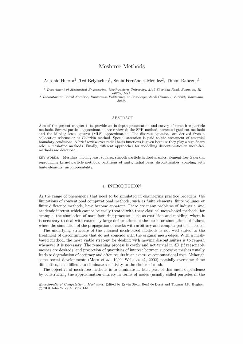
Figure 2. Cubic spline and corrected window function for polynomials of degree 2.
Rectangular supported window function:
φ(x) = φ1D(|x1|)φ1D(|x2|)
where, as usual, x = (x1, x2) and ‖x‖ =√x2
1 + x22.
2.1.3. Design of window functions In the continuous SPH approximation (1), a windowfunction φ can easily be modified to exactly reproduce a polynomial space Pm in R of degree≤ m, i.e.
p(x) =
∫Cρ φ
(y − x
ρ
)p(y) dy, ∀ p ∈ Pm. (6)
If the following conditions are satisfied∫Cρ φ
(yρ
)dy = 1,
∫Cρ φ
(yρ
)yj dy = 0 for 0 < j ≤ m
the window function is able to reproduce the polynomial space Pm. Note that the first conditioncoincides with (2) and defines the normalization constant, i.e. it imposes the reproducibilityof constant functions. These equations are often referred as consistency conditions although,a more appropriate term would be completeness conditions.
For example, the window function
φ(x) =
(27
17− 120
17x2
)φ(x), (7)
where φ(x) is the cubic spline, reproduces the second degree polynomial basis 1, x, x2. Figure2 shows the cubic spline defined in (4) and the corrected window function (7), see Liu et al.(1996b) for details.
Encyclopedia of Computational Mechanics. Edited by Erwin Stein, Rene de Borst and Thomas J.R. Hughes.
c© 2004 John Wiley & Sons, Ltd.
ECM005 7
−1 −0.5 0 0.5 1−0.5
0
0.5
1
1.5
2
2.5
−1 −0.5 0 0.5 1
−1
−0.5
0
0.5
1
u(x)=xurho(x)
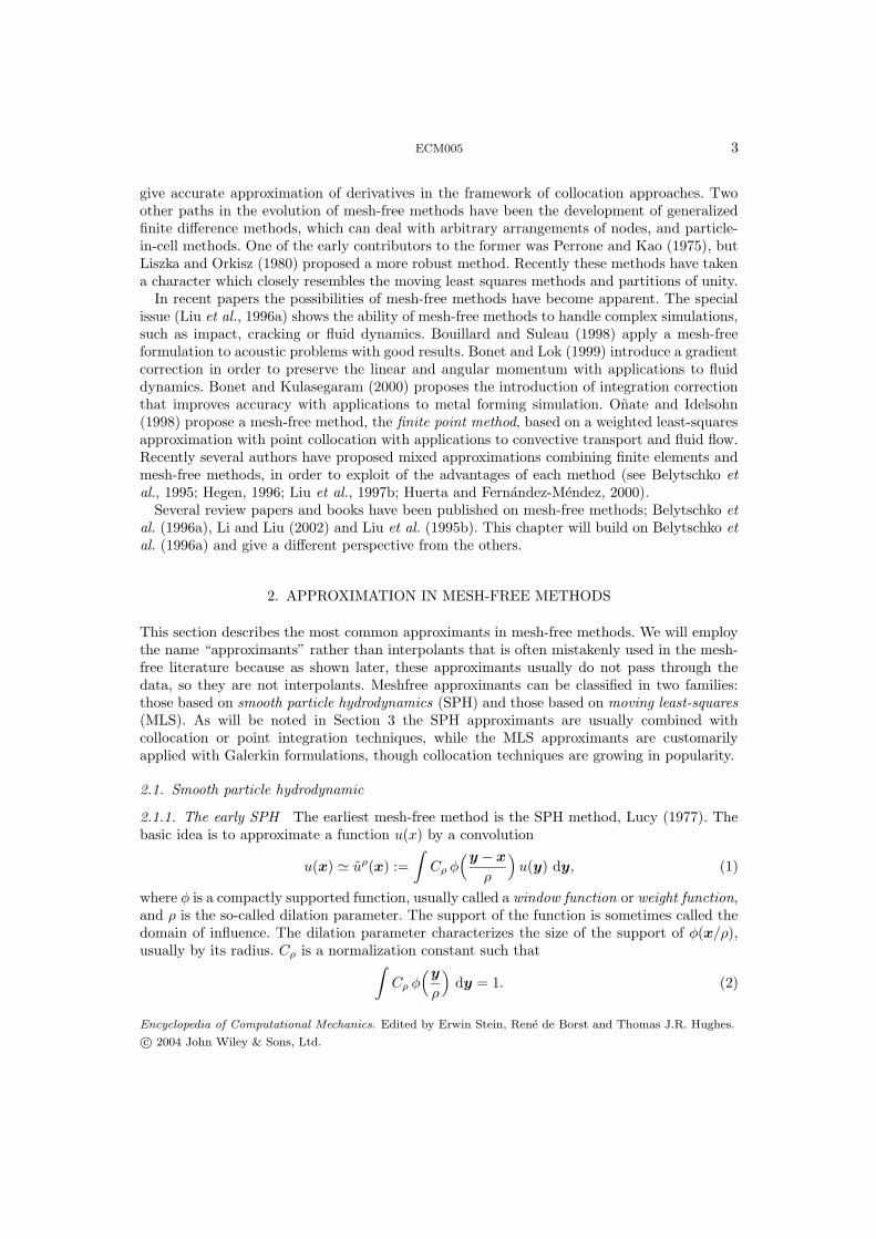
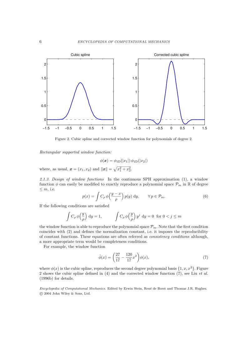
Figure 3. Modified cubic splines and particles, h = 0.5, and SPH discrete approximation for u(x) = xwith ρ/h = 2 in an “unbounded domain”.
−1 −0.5 0 0.5 1−0.5
0
0.5
1
1.5
2
2.5
−1 −0.5 0 0.5 1
−1
−0.5
0
0.5
1
u(x)=xurho(x)
Figure 4. Modified cubic splines and particles, h = 0.5, and SPH discrete approximation for u(x) = xwith ρ/h = 2 in a bounded domain.
However, the design of the window function is not trivial in the presence of boundariesor with nonuniform distributions of particles (see Section 2.2). Figure 3 shows the correctedcubic spline window functions associated with a uniform distribution of particles, with distanceh = 0.5 between particles and ρ = 2h, and the discrete SPH approximation described by (3) foru(x) = x with uniform weights ωI = h. The particles outside the interval [−1, 1] are consideredin the approximation, as in an unbounded domain (the corresponding translated windowfunctions are depicted with green). The linear monomial u(x) = x is exactly reproduced.However, in a bounded domain, the approximation is not exact near the boundaries when onlythe particles in the domain, [−1, 1] are considered in this example, see Figure 4.
Remark 5 (Consistency) If the approximation reproduces exactly a basis of the polynomialsof degree less or equal to m then the approximation is said to have m-order consistency.
2.1.4. Correcting the SPH method The SPH approximation is used in the solution of PDEs,usually through a collocation technique or point integration approaches, see Monaghan (1982),
Encyclopedia of Computational Mechanics. Edited by Erwin Stein, Rene de Borst and Thomas J.R. Hughes.
c© 2004 John Wiley & Sons, Ltd.

8 ENCYCLOPEDIA OF COMPUTATIONAL MECHANICS
Vila (1999), Bonet and Lok (1999) and Section 3.1. Thus, it is necessary to compute accurateapproximations of the derivatives of the dependent variables. The derivatives provided byoriginal SPH method can be quite inaccurate, and thus, it is necessary to improve theapproximation, or its derivatives, in some manner.
Randles and Libersky (1996), Krongauz and Belytschko (1998a) and Vila (1999) proposed acorrection of the gradient: the renormalized meshless derivative (RMD). It is an extension ofthe partial correction proposed by Johnson and Beissel (1996). Let the derivatives of a functionu be approximated as the derivatives of the SPH approximation defined in (3),
∇u(x) ' ∇uρ(x) =∑
I
∇ω(xI ,x)u(xI).
The basic idea of the RMD approximation is to define a corrected derivative
Dρu(x) :=∑
J
B(x)∇ω(xJ ,x)u(xJ ), (8)
where the correction matrix B(x) is chosen such that ∇u(x) = Dρu(x) for all linearpolynomials. In Vila (1999), a symmetrized approximation for the derivatives is defined
DρSu(x) := Dρu(x) −Dρ1(x) u(x), (9)
where, by definition (8),
Dρ1(x) =∑
J
B(x)∇ω(xJ ,x),
Note that (9) interpolates exactly the derivatives when u(x) is constant. The consistencycondition ∇u(x) = Dρ
Su(x) must be imposed only for linear monomials
B(x) =
[∑
J
∇ω(xJ ,x) (xJ − x)T]−1
.
If the ratio between the dilation parameter ρ and the distance between particles remainsconstant, there are a priori error bounds for the RMD, Dρ
Su, similar to the linear finiteelement ones, where ρ plays the role of the element size in finite elements, Vila (1999).
In SPH, the interparticle forces coincide with the vector joining them, so conservation oflinear and angular momentum are met for each point pair. In other words, linear and angularmomentum are conserved locally, see Dilts (1999).
When the kernels are corrected to reproduce linear polynomials or the derivatives oflinear polynomials, these local conservation properties are lost. However, global linear andtranslational momentum are conserved if the approximation reproduces linear functions, seeKrongauz and Belytschko (1998a) and Bonet and Lok (1999).
Although the capability to reproduce a polynomial of a certain order is an ingredient in manyconvergence proofs of solutions for PDEs, it does not suffice to pass the patch test. Krongauzand Belytschko (1998b) found that corrected gradient methods do not satisfy the patch testand exhibit poor convergence when the corrected gradient is used for the test function. Theyshowed that a Petrov-Galerkin method with Shepard test functions satisfies the patch test.
There are other ways of correcting the SPH method. For example, Bonet and Lok (1999)combine a correction of the window function, as in the RKPM method (see Section 2.2),
Encyclopedia of Computational Mechanics. Edited by Erwin Stein, Rene de Borst and Thomas J.R. Hughes.
c© 2004 John Wiley & Sons, Ltd.

ECM005 9
and a correction of the gradient to preserve angular momentum. In fact, there are a lot ofsimilarities between the corrected SPH and the renormalized meshless derivative. The mostimportant difference between the RMD approach where the 0-order consistency is obtained bythe definition of the symmetrized gradient (8), and the corrected gradient ∇uρ is that in thiscase 0-order consistency is obtained with the Shepard function.
With a similar rationale, Bonet and Kulasegaram (2000) present a correction of the windowfunction and an integration corrected vector for the gradients (in the context of metal formingsimulations). The corrected approximation is used in a weak form with numerical integrationat the particles (see Section 3.2). Thus, the gradient must be evaluated only at the particles.However, usually the particle integration is not accurate enough and the approximation failsto pass the patch test. In order to obtain a consistent approximation a corrected gradient isdefined. At every particle xI the corrected gradient is computed as
∇uρ(xI) = ∇uρ(xI) + γIJuKI
where γI is the correction vector (one component for each spatial dimension) at particle xI andwhere the bracket JuKI is defined as JuKI = u(xI) − uρ(xI). These extra parameters, γI , aredetermined requiring that the patch test be passed. A global linear system of equations mustbe solved to compute the correction vector and to define the derivatives of the approximation;then, the approximation of u and its derivatives are used to solve the boundary value problem.
2.2. Moving least-squares interpolants
2.2.1. Continuous moving least-squares The objective of the MLS approach is to obtain anapproximation similar to the SPH one (1), with high accuracy even in a bounded domain.Let us consider a bounded, or unbounded, domain Ω. The basic idea of the MLS approachis to approximate u(x), at a given point x, through a polynomial least-squares fit of u ina neighborhood of x. That is, for fixed x ∈ Ω, and z near x, u(z) is approximated with apolynomial expression
u(z) ' uρ(z,x) = PT(z) c(x) (10)
where the coefficients c(x) = c0(x), c1(x), . . . , cl(x)T are not constant, they depend onpoint x, and P(z) = p0(z), p1(z), . . . , pl(z)T includes a complete basis of the subspaceof polynomials of degree m. It can also include exact features of a solution, such as cracktipfields, as described in Ventura et al. (2002). The vector c(x) is obtained by a least-squares fit,with the scalar product
〈f, g〉x =
∫
Ω
φ(y − x
ρ
)f(y) g(y) dy. (11)
That is, the coefficients c are obtained by minimization of the functional Jx(c) centered in x
and defined by
Jx(c) =
∫
Ω
φ(y − x
ρ
)[u(y) − P(y) c(x)
]2dy, (12)
where φ((y−x)/ρ
)is the compact supported weighting function. The same weighting/window
functions as for SPH, given in Section 2.1.2, are used.
Remark 6. Thus, the scalar product is centered at the point x and scaled with the dilationparameter ρ. In fact, the integration is constructed in a neighborhood of radius ρ centered atx, that is, in the support of φ
((· − x)/ρ
).
Encyclopedia of Computational Mechanics. Edited by Erwin Stein, Rene de Borst and Thomas J.R. Hughes.
c© 2004 John Wiley & Sons, Ltd.
10 ENCYCLOPEDIA OF COMPUTATIONAL MECHANICS
Remark 7 (Polynomial space) In one dimension, we can let pi(x) be the monomials xi,and, in this particular case, l = m. For larger spatial dimensions two types of polynomialspaces are usually chosen: the set of polynomials, Pm, of total degree ≤ m, and the set ofpolynomials, Qm, of degree ≤ m in each variable. Both include a complete basis of the subspaceof polynomials of degree m. This, in fact, characterizes the a priori convergence rate, see Liuet al. (1997a) or Fernandez-Mendez et al. (2003).
The vector c(x) is the solution of the normal equations, that is, the linear system of equations
M(x) c(x) = 〈P, u〉x (13)
where M(x) is the Gram matrix (sometimes called a moment matrix) ,
M(x) =
∫
Ω
φ(y − x
ρ
)P(y)PT(y) dy. (14)
From (14) and (10), the least-squares approximation of u in a neighborhood of x is:
u(z) ' uρ(z,x) = PT(z) M−1(x)〈P, u〉x. (15)
Since the weighting function φ usually favors the central point x, it seems reasonable to assumethat such an approximation is more accurate precisely at z = x and thus the approximation(15) is particularized at x, that is,
u(x) ' uρ(x) := uρ(x,x) =
∫
Ω
φ(y − x
ρ
)PT(x) M−1(x) P(y) u(y) dy, (16)
where the definition of the scalar product, equation (11), has been explicitly used. Equation(16) can be rewritten as
u(x) ' uρ(x) =
∫
Ω
Cρ(y,x)φ(y − x
ρ
)u(y) dy,
which is similar to the SPH approximation, see equation (1), and with the scalar correctionterm Cρ(y,x) defined as
Cρ(y,x) := PT(x) M−1(x) P(y).
The function defined by the product of the correction and the window function φ,
Φ(y,x) := Cρ(y,x)φ(y − x
ρ
),
is usually called kernel function. The new correction term depends on the point x andthe integration variable y; it provides an accurate approximation even in the presence ofboundaries, see Liu et al. (1996b) for more details. In fact, the approximation verifies thefollowing consistency property, see also Wendland (2001).
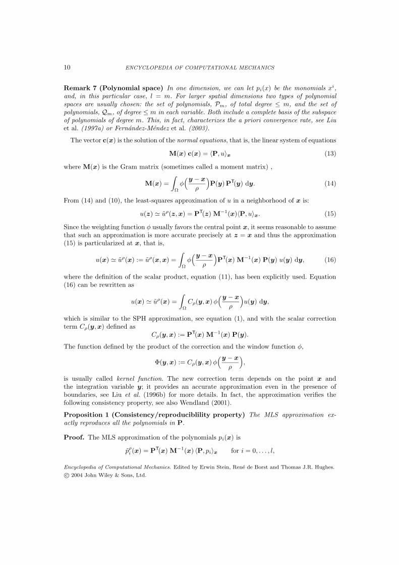
Proposition 1 (Consistency/reproduciblility property) The MLS approximation ex-actly reproduces all the polynomials in P.
Proof. The MLS approximation of the polynomials pi(x) is
pρi (x) = PT(x) M−1(x) 〈P, pi〉x for i = 0, . . . , l,
Encyclopedia of Computational Mechanics. Edited by Erwin Stein, Rene de Borst and Thomas J.R. Hughes.
c© 2004 John Wiley & Sons, Ltd.

ECM005 11
or, equivalently, in vector form
[Pρ
]T
(x) = PT(x) M−1(x)
∫
Ω
φ(y − x
ρ
)P(y)PT(y) dy
︸ ︷︷ ︸M(x)
.
Therefore, using the definition of M, see (14), it is trivial to verify that Pρ(x) ≡ P(x).
2.2.2. Reproducing kernel particle method approximation Application of a numericalquadrature in (16) leads to the reproducing kernel particle method (RKPM) approximation
u(x) ' uρ(x) ' uρ(x) :=∑
I∈Sρx
ω(xI ,x)PT(x) M−1(x) P(xI) u(xI),
where ω(xI ,x) = ωI φ((xI − x)/ρ
)and xI and ωI are integration points (particles) and
weights, respectively. The particles cover the computational domain Ω, Ω ⊂ Rnsd . Let Sρx be
the index set of particles whose support include the point x, see Remark 9. This approximationcan be written as
u(x) ' uρ(x) =∑
I∈Sx
NI(x)u(xI) (17)
where the approximation functions are defined by
NI(x) = ω(xI ,x)PT(x) M−1(x) P(xI). (18)
Remark 8. In order to preserve the consistency/reproducibility property, the matrix M,defined in (14), must be evaluated with the same quadrature used in the discretization of (16),see Chen et al. (1996) for details. That is, matrix M(x) must be computed as
M(x) =∑
I∈Sρx
ω(xI ,x)P(xI)PT(xI). (19)
Remark 9. The sums in (17) and (19) only involve the indices I such that φ(xI ,x) 6= 0, thatis, particles xI in a neighborhood of x. Thus, the set of neighboring particles is defined by theset of indices
Sρx
:= J such that ‖xJ − x‖ ≤ ρ.Remark 10 (Conditions on particle distribution) The matrix M(x) in (19) must beregular at every point x in the domain. Liu et al. (1997a) discuss the necessary conditions.In fact, this matrix can be viewed, see Huerta and Fernandez-Mendez (2000) or Fernandez-Mendez and Huerta (2002), as a Gram matrix defined with a discrete scalar product
〈f, g〉x =∑
I∈Sρx
ω(xI ,x) f(xI) g(xI). (20)
If this scalar product is degenerated, M(x) is singular. Regularity of M(x) is ensured by havingenough particles in the neighborhood of every point x and avoiding degenerate patterns, that is
(i) card Sρx ≥ l + 1.
(ii) @F ∈ spanp0, p1, . . . , pl \ 0 such that F (xI) = 0 ∀ I ∈ Sρx.
Encyclopedia of Computational Mechanics. Edited by Erwin Stein, Rene de Borst and Thomas J.R. Hughes.
c© 2004 John Wiley & Sons, Ltd.

12 ENCYCLOPEDIA OF COMPUTATIONAL MECHANICS
Condition (ii) is easily verified. For instance, for m = 1 (linear interpolation) the particlescannot lie in the same straight line or plane for, respectively, 2D and 3D. In 1D, for any valueof m, it suffices that different particles do not have the same position. Under these conditionsone can compute the vector PT(x)M−1(x) at each point and thus determine, from (18), theshape functions, NI(x).
2.2.3. Discrete MLS: element-free Galerkin approximation The MLS development, alreadypresented in Section 2.2.1 for the continuous case (i.e. using integrals), can be developeddirectly from a discrete formulation. As in the continuous case, the idea is to approximateu(x), at a given point x, by a polynomial least-squares fit of u in a neighborhood of x. Thatis, the same expression presented in (10) can be used, namely for fixed x ∈ Ω, and z near x,u(z) is approximated with the polynomial expression
u(z) ' uρ(z,x) = PT(z) c(x). (21)
In the framework of the element-free Galerkin (EFG) method, the vector c(x) is also obtainedby a least-squares fit, with the discrete scalar product defined in (20), where ω(xI ,x) is thediscrete weighting function, which is equivalent to the window function
ω(xI ,x) = φ(xI − x
ρ
), (22)
and Sρx
is the set of indices of neighboring particles defined in Remark 9. That is, the coefficientsc are obtained by minimization of the discrete functional Jx(c) centered in x and defined by
Jx(c) =∑
I∈Sρx
ω(xI ,x)[u(xI) − P(xI) c(x)
]2. (23)
The normal equations are defined in a similar manner,
M(x) c(x) = 〈P, u〉x, (24)
and the Gram matrix is directly obtained from the discrete scalar product, see equation (19).After substitution of the solution of (24) in (21), the least-squares approximation of u in aneighborhood of x is obtained
u(z) ' uρ(z,x) = PT(z)M−1(x)∑
I∈Sρx
ω(xI ,x)P(xI)u(xI). (25)
Particularization of (25) at z = x leads to the discrete MLS approximation of u(x)
u(x) ' uρ(x) := uρ(x,x) =∑
I∈Sρx
ω(xI ,x)PT(x) M−1(x) P(xI)u(xI). (26)
This EFG approximation coincides with the RKPM one described in equations (18) and (19).
Remark 11 (Convergence) Liu et al. (1997a) showed convergence of the RKPM and EFG.The a priori error bound is very similar to the bound in finite elements. The parameter ρ playsthe role of h, and m (the order of consistency) plays the role of the degree of the approximationpolynomials in the finite element mesh. Convergence properties depend on m and ρ. They donot depend on the distance between particles because usually this distance is proportional to ρ,i.e. the ratio between the particle distance over the dilation parameter is of order one, see Liuet al. (1997a).
Encyclopedia of Computational Mechanics. Edited by Erwin Stein, Rene de Borst and Thomas J.R. Hughes.
c© 2004 John Wiley & Sons, Ltd.

ECM005 13
Figure 5. Interpolation functions with ρ/h ' 1 (similar to finite elements) and ρ/h = 2.6, with cubicspline and linear consistency.
NI (NI)x (NI)xx
Linear FE
0 0.1 0.2 0.3 0.4 0.5 0.6 0.7 0.8 0.9 1−0.2
0
0.2
0.4
0.6
0.8
1
0 0.1 0.2 0.3 0.4 0.5 0.6 0.7 0.8 0.9 1
−10
−5
0
5
10
Dirac deltafunctions
EFG, ρ/h = 3.2
P(x) = 1, xT
0 0.1 0.2 0.3 0.4 0.5 0.6 0.7 0.8 0.9 1−0.2
0
0.2
0.4
0.6
0.8
1
0 0.1 0.2 0.3 0.4 0.5 0.6 0.7 0.8 0.9 1−3
−2
−1
0
1
2
3
0 0.1 0.2 0.3 0.4 0.5 0.6 0.7 0.8 0.9 1−50
−40
−30
−20
−10
0
10
20
30
EFG, ρ/h = 3.2
P(x) =1, x, x2T
0 0.1 0.2 0.3 0.4 0.5 0.6 0.7 0.8 0.9 1−0.2
0
0.2
0.4
0.6
0.8
1
0 0.1 0.2 0.3 0.4 0.5 0.6 0.7 0.8 0.9 1−8
−6
−4
−2
0
2
4
6
8
0 0.1 0.2 0.3 0.4 0.5 0.6 0.7 0.8 0.9 1−150
−100
−50
0
50
100
Figure 6. Shape function and derivatives for linear finite elements and the EFG approximation.
Remark 12. The approximation is characterized by the order of consistency required, i.e. thecomplete basis of polynomials employed in P, and by the ratio between the dilation parameterand the particle distance, ρ/h. In fact, the bandwidth of the stiffness matrix increases withthe ratio ρ/h (more particles lie inside the circle of radius ρ), see for instance Figure 5. Notethat, for linear consistency, when ρ/h goes to 1, the linear finite element shape functions arerecovered.
Remark 13 (Continuity) If the weight function φ is Ck then the EFG/MLS shape functions,and the RKPM shape functions, are Ck, see Liu et al. (1997a). Thus, if the window functionis a cubic spline, as shown in Figures 6 and 7, the first and second derivatives of the shapefunctions are well defined throughout the domain, even with linear consistency.
Encyclopedia of Computational Mechanics. Edited by Erwin Stein, Rene de Borst and Thomas J.R. Hughes.
c© 2004 John Wiley & Sons, Ltd.

14 ENCYCLOPEDIA OF COMPUTATIONAL MECHANICS
00.5
1
00.5
10
0.2
0.4
x
Ni
y 00.5
1
00.5
1−1
0
1
x
(Ni)x
y
00.5
1
00.5
1−1
0
1
x
(Ni)y
y
00.5
1
00.5
1−20
−10
0
10
x
(Ni)xx
y
00.5
1
00.5
1−20
−10
0
10
x
(Ni)yy
y
Figure 7. Distribution of particles, EFG approximation function and derivatives, with ρ/h ' 2.2 withcircular supported cubic spline and linear consistency.
2.2.4. Reproducibility of the MLS approximation The MLS shape functions can be alsoobtained by imposing a priori the reproducibility properties of the approximation. Consider aset of particles xI and a complete polynomial base P(x). Let us assume an approximation ofthe form
u(x) '∑
I∈Sρx
NI(x)u(xI), (27)
with approximation functions defined as
NI(x) = ω(xI ,x)PT(xI) α(x). (28)
The unknown vector α(x) in Rl+1 is determined imposing the reproducibility condition, whichimposes that the approximation proposed in (27) is exact for all the polynomials in P, namely
P(x) =∑
J∈Sρx
NJ(x)P(xJ). (29)
After substitution of (28) in (29), the linear system of equations that determines α(x) isobtained
M(x) α(x) = P(x). (30)
That is,α(x) = M−1(x)P(x), (31)
Encyclopedia of Computational Mechanics. Edited by Erwin Stein, Rene de Borst and Thomas J.R. Hughes.
c© 2004 John Wiley & Sons, Ltd.
ECM005 15
where M(x) is the same matrix defined in (19). Finally, the approximation functions NI(x)are defined by substituting in (28) the vector α, see (31). Note that with this substitution theexpression (18) for the MLS approximation functions is recovered, and consistency is ensuredby construction.
Section 2.2.7 is devoted to some implementation details of the EFG method. In particular,it is shown that the derivatives of NI(x) can be computed without excessive overhead.
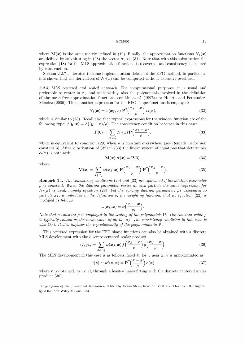
2.2.5. MLS centered and scaled approach For computational purposes, it is usual andpreferable to center in xJ and scale with ρ also the polynomials involved in the definitionof the mesh-free approximation functions, see Liu et al. (1997a) or Huerta and Fernandez-Mendez (2000). Thus, another expression for the EFG shape functions is employed:
NI(x) = ω(xI ,x) PT
(xI − x
ρ
)α(x), (32)
which is similar to (28). Recall also that typical expressions for the window function are of thefollowing type: φ(y,x) = φ
((y − x)/ρ
). The consistency condition becomes in this case:
P(0) =∑
I∈Sρx
NI(x)P(xI − x
ρ
), (33)
which is equivalent to condition (29) when ρ is constant everywhere (see Remark 14 for nonconstant ρ). After substitution of (32) in (33) the linear system of equations that determinesα(x) is obtained:
M(x) α(x) = P(0), (34)
where
M(x) =∑
J∈Sρx
ω(xJ ,x) P(xJ − x
ρ
)PT
(xJ − x
ρ
). (35)
Remark 14. The consistency conditions (29) and (33) are equivalent if the dilation parameterρ is constant. When the dilation parameter varies at each particle the same expression forNI(x) is used, namely equation (28), but the varying dilation parameter, ρI associated toparticle xI , is imbedded in the definition of the weighting function; that is, equation (22) ismodified as follows
ω(xI ,x) = φ(xI − x
ρI
).
Note that a constant ρ is employed in the scaling of the polynomials P. The constant value ρis typically chosen as the mean value of all the ρJ . The consistency condition in this case isalso (33). It also imposes the reproducibility of the polynomials in P.
This centered expression for the EFG shape functions can also be obtained with a discreteMLS development with the discrete centered scalar product
〈f, g〉x =∑
J∈Sρx
ω(xJ ,x) f(xJ − x
ρ
)g(xJ − x
ρ
). (36)
The MLS development in this case is as follows: fixed x, for z near x, u is approximated as
u(z) ' uρ(z,x) = PT
(z − x
ρ
)c(x) (37)
where c is obtained, as usual, through a least-squares fitting with the discrete centered scalarproduct (36).
Encyclopedia of Computational Mechanics. Edited by Erwin Stein, Rene de Borst and Thomas J.R. Hughes.
c© 2004 John Wiley & Sons, Ltd.
16 ENCYCLOPEDIA OF COMPUTATIONAL MECHANICS
2.2.6. The diffuse derivative The centered MLS allows, with a proper definition of thepolynomial basis P, the reinterpretation of the coefficients in c(x) as approximations of uand its derivatives at the fixed point x.
The approximation of the derivative of u in each spatial direction is the correspondingderivative of uρ. This requires to derive (21), that is
∂u
∂x' ∂uρ
∂x=∂PT
∂xc + PT
∂c
∂x. (38)
On one hand, the second term on the r.h.s. is not trivial. Derivatives of the coefficientsc require the resolution of a linear system of equations with the same matrix M. As notedby Belytschko et al. (1996b) this is not an expensive task, see also Section 2.2.7. However, itrequires the knowledge of the cloud of particles surrounding each point x, and, thus, it dependson the point where derivatives are evaluated.
On the other hand, the first term is easily evaluated. The derivative of the polynomials in Pis trivial and can be evaluated a priori, without knowledge of the cloud of particles surroundingeach point x.
Villon (1991) and Nayroles et al. (1992) propose the concept of diffuse derivative, whichconsists in approximating the derivative only with the first term on the r.h.s. of (38), namely
δuρ
δx=∂uρ
∂z
∣∣∣∣z=x
=∂PT
∂z
∣∣∣∣z=x
c(x) =∂PT
∂xc(x).
From a computational cost point of view, this is an interesting alternative to (38). Moreover,the following proposition ensures convergence at optimal rate of the diffuse derivative.
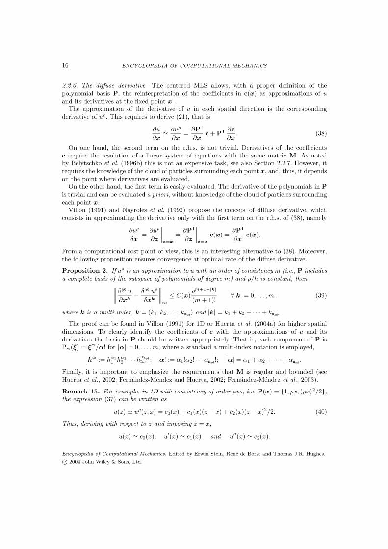
Proposition 2. If uρ is an approximation to u with an order of consistency m (i.e., P includesa complete basis of the subspace of polynomials of degree m) and ρ/h is constant, then
∥∥∥∥∂|k|u
∂xk− δ|k|uρ
δxk
∥∥∥∥∞
≤ C(x)ρm+1−|k|
(m+ 1)!∀|k| = 0, . . . ,m. (39)
where k is a multi-index, k = (k1, k2, . . . , knsd) and |k| = k1 + k2 + · · · + knsd.
The proof can be found in Villon (1991) for 1D or Huerta et al. (2004a) for higher spatialdimensions. To clearly identify the coefficients of c with the approximations of u and itsderivatives the basis in P should be written appropriately. That is, each component of P isPα(ξ) = ξα/α! for |α| = 0, . . . ,m, where a standard a multi-index notation is employed,
hα := hα1
1 hα2
2 · · ·hαnsd
nsd; α! := α1!α2! · · ·αnsd
!; |α| = α1 + α2 + · · · + αnsd.
Finally, it is important to emphasize the requirements that M is regular and bounded (seeHuerta et al., 2002; Fernandez-Mendez and Huerta, 2002; Fernandez-Mendez et al., 2003).
Remark 15. For example, in 1D with consistency of order two, i.e. P(x) = 1, ρx, (ρx)2/2,the expression (37) can be written as
u(z) ' uρ(z, x) = c0(x) + c1(x)(z − x) + c2(x)(z − x)2/2. (40)
Thus, deriving with respect to z and imposing z = x,
u(x) ' c0(x), u′(x) ' c1(x) and u′′(x) ' c2(x).
Encyclopedia of Computational Mechanics. Edited by Erwin Stein, Rene de Borst and Thomas J.R. Hughes.
c© 2004 John Wiley & Sons, Ltd.
ECM005 17
In fact, this strategy is at the basis of the diffuse element method : the diffuse derivative is usedin the weak form of the problem (see Nayroles et al., 1992; Breitkopf et al., 2001). Moreover,the generalized finite difference interpolation or meshless finite difference method, see Orkisz(1998), coincides also with this MLS development. The only difference between the generalizedfinite difference interpolation and the EFG centered interpolation is the definition of the setof neighboring particles Sρ
x.
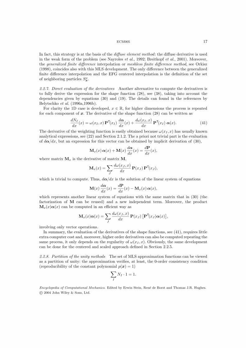
2.2.7. Direct evaluation of the derivatives Another alternative to compute the derivatives isto fully derive the expression for the shape function (28), see (38), taking into account thedependencies given by equations (30) and (19). The details can found in the references byBelytschko et al. (1996a,1996b).
For clarity the 1D case is developed, x ∈ R, for higher dimensions the process is repeatedfor each component of x. The derivative of the shape function (28) can be written as
dNI
dx(x) = ω(xI , x)P
T(xI)dα
dx(x) +
dω(xI , x)
dxPT(xI) α(x). (41)
The derivative of the weighting function is easily obtained because ω(xI , x) has usually knownanalytical expressions, see (22) and Section 2.1.2. The a priori not trivial part is the evaluationof dα/dx, but an expression for this vector can be obtained by implicit derivation of (30),
Mx(x)α(x) + M(x)dα
dx(x) =
dP
dx(x),
where matrix Mx is the derivative of matrix M,
Mx(x) =∑
J
dω(xJ , x)
dxP(xJ)PT(xJ ),
which is trivial to compute. Thus, dα/dx is the solution of the linear system of equations
M(x)dα
dx(x) =
dP
dx(x) − Mx(x)α(x),
which represents another linear system of equations with the same matrix that in (30) (thefactorization of M can be reused) and a new independent term. Moreover, the productMx(x)α(x) can be computed in an efficient way as
Mx(x)α(x) =∑
J
dω(xJ , x)
dxP(xJ )
[PT(xJ )α(x)
],
involving only vector operations.In summary, the evaluation of the derivatives of the shape functions, see (41), requires little
extra computer cost and, moreover, higher order derivatives can also be computed repeating thesame process, it only depends on the regularity of ω(xI , x). Obviously, the same developmentcan be done for the centered and scaled approach defined in Section 2.2.5.
2.2.8. Partition of the unity methods The set of MLS approximation functions can be viewedas a partition of unity: the approximation verifies, at least, the 0-order consistency condition(reproducibility of the constant polynomial p(x) = 1)
∑
I
NI · 1 = 1.
Encyclopedia of Computational Mechanics. Edited by Erwin Stein, Rene de Borst and Thomas J.R. Hughes.
c© 2004 John Wiley & Sons, Ltd.
18 ENCYCLOPEDIA OF COMPUTATIONAL MECHANICS
This viewpoint leads to new approximations for mesh-free methods. Based on the partition ofthe unity finite element method (PUFEM) proposed by Babuska and Melenk (1995), Duarteand Oden (1996a) use the concept of partition of unity to construct approximations withconsistency of order k ≥ 1. They called their method h-p clouds. The approximation is
u(x) ' uρ(x) =∑
I
NI(x)uI +∑
I
nI∑
i=1
bIi
[NI(x) qIi(x)
],
where NI(x) are the MLS approximation functions, qIi are nI polynomials of degree greaterthan k associated to each particle xI , and uI , bIi are coefficients to determine. Note that thepolynomials qIi(x) increase the order of the approximation space. These polynomials can bedifferent from particle to particle, thus facilitating the hp-adaptivity.
Remark 16. As commented in Belytschko et al. (1996a), the concept of an extrinsic basis,qIi(x), is essential for obtaining p-adaptivity. In MLS approximations, the intrinsic basis Pcannot vary form particle to particle without introducing a discontinuity.
3. DISCRETIZATION OF PARTIAL DIFFERENTIAL EQUATIONS
All the approximation functions described in the previous section can be used in the solutionof a PDE boundary value problem. Usually SPH methods are combined with collocation orpoint integration technique, while the approximations based on MLS are usually combinedwith a Galerkin discretization.
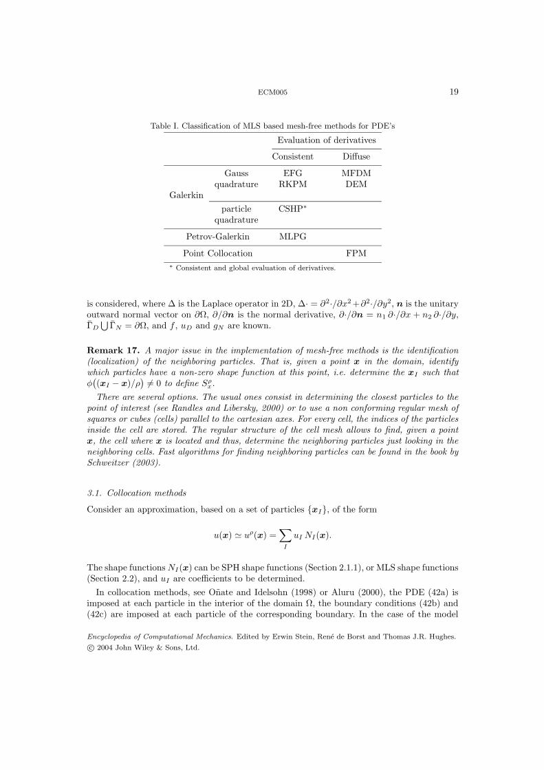
A large number of published methods with minor differences exist. Probably, the best known,among those using MLS approximation, are: the meshless (generalized) finite difference method(MFDM) developed by Liszka and Orkisz (1980), the diffuse element method (DEM) byNayroles et al. (1992), the element-free Galerkin (EFG) method by Belytschko et al. (1994), thereproducing kernel particle method (RKPM) by Liu et al. (1995a), the meshless local Petrov-Galerkin (MLPG) by Zhu and Atluri (1998), the corrected smooth particle hydrodynamics(CSPH) by Bonet and Lok (1999) and the finite point method (FPM) by Onate and Idelsohn(1998). Table I classifies these methods depending on the evaluation of the derivatives (seeSections 2.2.6 and 2.2.7) and how the PDE is solved (Galerkin, Petrov-Galerkin, pointcollocation).
Partition of unity methods can be implemented with Galerkin, Petrov-Galerkin, etc. Forinstance, the h−p clouds by Duarte and Oden (1996a) use a Galerkin weak form with accurateintegration, while the finite spheres by De and Bathe (2000) uses Shepard functions (withcircular/spherical support) enriched with polynomials and a Galerkin weak form with specificquadratures for spherical domains (and particular/adapted quadratures near the boundary);almost identical to h-p clouds Duarte and Oden (1996a).
In order to discuss some of these methods in more detail, the model boundary value problem
∆u− u = −f in Ω (42a)
u = uD on ΓD (42b)
∂u
∂n= gN on ΓN (42c)
Encyclopedia of Computational Mechanics. Edited by Erwin Stein, Rene de Borst and Thomas J.R. Hughes.
c© 2004 John Wiley & Sons, Ltd.
ECM005 19
Table I. Classification of MLS based mesh-free methods for PDE’s
Evaluation of derivatives
Consistent Diffuse
Gauss EFG MFDMquadrature RKPM DEM
Galerkin
particle CSHP∗
quadrature
Petrov-Galerkin MLPG
Point Collocation FPM
∗ Consistent and global evaluation of derivatives.
is considered, where ∆ is the Laplace operator in 2D, ∆· = ∂2·/∂x2 +∂2·/∂y2, n is the unitaryoutward normal vector on ∂Ω, ∂/∂n is the normal derivative, ∂·/∂n = n1 ∂·/∂x + n2 ∂·/∂y,ΓD
⋃ΓN = ∂Ω, and f , uD and gN are known.
Remark 17. A major issue in the implementation of mesh-free methods is the identification(localization) of the neighboring particles. That is, given a point x in the domain, identifywhich particles have a non-zero shape function at this point, i.e. determine the xI such thatφ((xI − x)/ρ
)6= 0 to define Sρ
x.
There are several options. The usual ones consist in determining the closest particles to thepoint of interest (see Randles and Libersky, 2000) or to use a non conforming regular mesh ofsquares or cubes (cells) parallel to the cartesian axes. For every cell, the indices of the particlesinside the cell are stored. The regular structure of the cell mesh allows to find, given a pointx, the cell where x is located and thus, determine the neighboring particles just looking in theneighboring cells. Fast algorithms for finding neighboring particles can be found in the book bySchweitzer (2003).
3.1. Collocation methods
Consider an approximation, based on a set of particles xI, of the form
u(x) ' uρ(x) =∑
I
uI NI(x).
The shape functionsNI(x) can be SPH shape functions (Section 2.1.1), or MLS shape functions(Section 2.2), and uI are coefficients to be determined.
In collocation methods, see Onate and Idelsohn (1998) or Aluru (2000), the PDE (42a) isimposed at each particle in the interior of the domain Ω, the boundary conditions (42b) and(42c) are imposed at each particle of the corresponding boundary. In the case of the model
Encyclopedia of Computational Mechanics. Edited by Erwin Stein, Rene de Borst and Thomas J.R. Hughes.
c© 2004 John Wiley & Sons, Ltd.

20 ENCYCLOPEDIA OF COMPUTATIONAL MECHANICS
problem, this leads to the linear system of equations for the coefficients uI :
∑
I
uI
[∆NI(xJ) −NI(xJ )
]= −f(xJ ) ∀xJ ∈ Ω,
∑
I
uI NI(xJ) = uD(xJ) ∀xJ ∈ ΓD,
∑
I
uI∂NI
∂n(xJ) = gN (xJ) ∀xJ ∈ ΓN .
Note that, the shape functions must be C2, and thus, a C2 window function must be used. Inthis case the solution at particle xJ is approximated by
u(xJ) ' uρ(xJ) =∑
I
uINI(xJ),
which in general differs from the coefficient uJ (see Remark 1).In the context of the renormalized meshless derivative (see Vila, 1999) the coefficient uJ is
considered as the approximation at the particle xJ and only the derivative of the solution isapproximated through the RMD, see (9). Thus, the linear system to be solved becomes
∑
I
uI ∆NI(xJ) − uJ = −f(xJ) ∀xJ ∈ Ω,
uJ = uD(xJ) ∀xJ ∈ ΓD,∑
I
uI∂NI
∂n(xJ) = gN (xJ) ∀xJ ∈ ΓN .
Both possibilities are slightly different from the SPH method by Monaghan (1988) or fromSPH methods based on particle integration techniques Bonet and Kulasegaram (2000).
3.2. Methods based on a Galerkin weak form
The mesh-free shape functions can also be used in the discretization of the weak integral formof the boundary value problem. For the model problem (42), the Bubnov-Galerkin weak form(also used in the finite element method) is
∫
Ω
∇v∇u dΩ +
∫
Ω
v u dΩ =
∫
Ω
v f dv +
∫
ΓN
v gN dΓ ∀v,
where v vanishes at ΓD and u = uD at ΓD. However, this weak form can not be directlydiscretized with a standard mesh-free approximation. The shape functions do not verify theKronecker delta property (see Remark 1) and thus, it is difficult to select v such that v = 0at ΓD and to impose that uρ = uD at ΓD. Specific techniques are needed in order to imposeDirichlet boundary conditions. Section 3.3 describes to the treatment of essential boundaryconditions in mesh-free methods.
An important issue in the implementation of a mesh-free method with a weak form is theevaluation of integrals in the weak form (the concept of finite element, with a numericalquadrature in each element can not be adopted directly).
Several possibilities can be considered to evaluate integrals in the weak form: (1) the particlescan be the quadrature points (particle integration), (2) a regular cell structure (for instance,
Encyclopedia of Computational Mechanics. Edited by Erwin Stein, Rene de Borst and Thomas J.R. Hughes.
c© 2004 John Wiley & Sons, Ltd.

ECM005 21
the same used for the localization of particles) can be used with numerical quadrature in eachcell (cell integration) or (3) a, not necessary regular, background mesh can be used to computeintegrals. The first possibility (particle integration) is the fastest, but as in collocation methodsit can result in rank deficiency. Bonet and Kulasegaram (2000) propose a global correction toobtain accurate and stable results with particle integration. The other two possibilities presentthe disadvantage that, since shape functions and their derivatives, are not polynomials, thenumber of integration points leads to high computational costs. Nevertheless, the cell structureor the coarse background mesh, which do not need to be conforming, are easily generated andthese techniques ensure an accurate approximation of the integrals.
3.3. Essential boundary conditions
Many specific techniques have been developed in the recent years in order to impose essentialboundary conditions in mesh-free methods. Some possibilities are: (1) Lagrange multipliers(Belytschko et al., 1994), (2) modified variational principles (Belytschko et al., 1994), (3)penalty methods (Zhu and Atluri, 1998; Bonet and Kulasegaram, 2000), (4) perturbedLagrangian (Chu and Moran, 1995), (5) coupling to finite elements (Belytschko et al., 1995;Huerta and Fernandez-Mendez, 2000; Wagner and Liu, 2001), or (6) modified shape functions(Gosz and Liu, 1996; Gunter and Liu, 1998; Wagner and Liu, 2000) among others.
The first attempts to define shape functions with the “delta property” along the boundary(see Gosz and Liu, 1996), namely NI(xJ) = δIJ for all xJ in ΓD, have serious difficulties forcomplex domains and for the integration of the weak forms.
In the recent years, mixed interpolations that combine finite elements with mesh-freemethods have been developed. Mixed interpolations can be quite effective for imposing essentialboundary conditions. The idea is to use one or two layers of finite elements next to the Dirichletboundary and use a mesh-free approximation in the rest of the domain. Thus, the essentialboundary conditions can be imposed as in standard finite elements. In Belytschko et al. (1995)a mixed interpolation is defined in the transition area (from the finite elements region to theparticles region). This mixed interpolation requires the substitution of finite element nodes byparticles and the definition of ramp functions. Thus, the transition is of the size of one elementand the interpolation is linear. Following this idea, Huerta and Fernandez-Mendez (2000)propose a more general mixed interpolation, with any order of interpolation, with no need forramp functions and no substitution of nodes by particles. This is done preserving consistencyand continuity of the solution. Figure 8 shows an example of this mixed interpolation in 1D: twofinite element nodes are considered at the boundary of the domain, with their correspondingshape functions in blue, and the mesh-free shape functions are modified in order to preserveconsistency, in black. The details of this method are presented in Section 6.
3.3.1. Methods based on a modification of the weak form For the sake of clarity, the followingmodel problem is considered
−∆u = f in Ω
u = uD on ΓD
∇u · n = gN on ΓN
(43)
where ΓD∪ΓN = ∂Ω, ΓD∩ΓN = ∅ and n is the outward unit normal on ∂Ω. The generalizationof the following developments to other PDEs is straightforward.
Encyclopedia of Computational Mechanics. Edited by Erwin Stein, Rene de Borst and Thomas J.R. Hughes.
c© 2004 John Wiley & Sons, Ltd.

22 ENCYCLOPEDIA OF COMPUTATIONAL MECHANICS
0 0.1 0.2 0.3 0.4 0.5 0.6 0.7 0.8 0.9 1
0
0.2
0.4
0.6
0.8
1
Figure 8. Mixed interpolation with linear finite element nodes near the boundary and particles in theinterior of the domain, with ρ/h = 3.2, cubic spline and linear consistency in all the domain.
The weak problem form of (43) is “find u ∈ H1(Ω) such that u = uD on ΓD and∫
Ω
∇v · ∇u dΩ −∫
ΓD
v∇u · n dΓ =
∫
Ω
vf dΩ +
∫
ΓN
vgN dΓ, (44)
for all v ∈ H1(Ω)”. In the finite element method, the interpolation of u can easily be forcedto verify the essential boundary condition, and the test functions v can be chosen such thatv = 0 on ΓD (see Remark 18), leading to the following weak form: “find u ∈ H1(Ω) such thatu = uD on ΓD and ∫
Ω
∇v · ∇u dΩ =
∫
Ω
vf dΩ +
∫
ΓN
vgN dΓ, (45)
for all v ∈ H10(Ω)”, where H1
0(Ω) = v ∈ H1(Ω) | v = 0 on ΓD.Remark 18. In the finite element method, or in the context of the continuous blending methoddiscussed in Section 6, the approximation can be written as
u(x) '∑
j /∈B
ujNj(x) + ψ(x) (46)
where Nj(x) denote the shape functions, ψ(x) =∑
j∈B uD(xj)Nj(x), and B is the set of indexesof all nodes on the essential boundary. Note that, due to the Kronecker delta property of theshape functions for i ∈ B, and the fact that Ni ∈ H1
0(Ω) for i /∈ B, the approximation definedby (46) verifies u = uD at the nodes on the essential boundary. Therefore, approximation (46)and v = Ni, for i /∈ B, can be considered for the discretization of the weak form (45). Underthese circumstances, the system of equations becomes
Ku = f , (47)
where
Kij =
∫
Ω
∇Ni · ∇Nj dΩ,
fi =
∫
Ω
Nif dΩ +
∫
Ω
Niψ dΩ +
∫
ΓN
NigN dΓ,
(48)
and u is the vector of coefficients ui.
Encyclopedia of Computational Mechanics. Edited by Erwin Stein, Rene de Borst and Thomas J.R. Hughes.
c© 2004 John Wiley & Sons, Ltd.
ECM005 23
However, for standard mesh-free approximation, the shape functions do not verify theKronecker delta property and Ni /∈ H1
0(Ω) for i /∈ B. Therefore, imposing u = uD and v = 0on ΓD is not as straightforward as in finite elements or as in the blending method (Belytschkoet al., 1995), and the weak form defined by (45) cannot be used. The most popular methodsthat modify the weak form to overcome this problem are: the Lagrange multiplier method, thepenalty method and Nitsche’s method.
3.3.2. Lagrange multiplier method The solution of problem (43) can also be obtained as thesolution of a minimization problem with constraints: “u minimizes the energy functional
Π(v) =1
2
∫
Ω
∇v · ∇v dΩ −∫
Ω
vf dΩ −∫
ΓN
vgN dΓ, (49)
and verifies the essential boundary conditions.” That is,
u = arg minv∈H1(Ω)
v=uD on ΓD
Π(v). (50)
With the use of a Lagrange multiplier, λ(x) , this minimization problem can also be writtenas
(u, λ) = arg minv∈H1(Ω)
maxγ∈H−1/2(ΓD)
Π(v) +
∫
ΓD
γ(v − uD) dΓ.
This min-max problem leads to the following weak form with Lagrange multiplier, “findu ∈ H1(Ω) and λ ∈ H−1/2(ΓD) such that
∫
Ω
∇v · ∇u dΩ +
∫
ΓD
vλ dΓ =
∫
Ω
vf dΩ +
∫
ΓN
vgN dΓ, ∀ v ∈ H1(Ω) (51a)
∫
ΓD
γ(u− uD) dΓ = 0, ∀ γ ∈ H− 12 (ΓD).” (51b)
Remark 19. Equation (51b) imposes the essential boundary condition, u = uD on ΓD, inweak form.
Remark 20. The physical interpretation of the Lagrange multiplier can be seen by simplecomparison of equations (51a) and (44): the Lagrange multiplier corresponds to the flux(traction in a mechanical problem) along the essential boundary, λ = −∇u · n.
Considering now the approximation u(x) ' ∑iNi(x)ui, with mesh-free shape functions Ni,
and an interpolation for λ with a set of boundary functions NLi (x)`
i=1,
λ(x) '∑
i=1
λiNLi (x) for x ∈ ΓD, (52)
the discretization of (51) leads to the system of equations(K AT
A 0
) (uλ
)=
(fb
), (53)
where K and f are already defined in (48) (use ψ = 0), λ is the vector of coefficients λi, and
Aij =
∫
ΓD
NLi Nj dΓ, bi =
∫
ΓD
NLi uD dΓ.
Encyclopedia of Computational Mechanics. Edited by Erwin Stein, Rene de Borst and Thomas J.R. Hughes.
c© 2004 John Wiley & Sons, Ltd.
24 ENCYCLOPEDIA OF COMPUTATIONAL MECHANICS
There are several possibilities for the choice of the interpolation space for the Lagrangemultiplier λ. Some of them are (1) a finite element interpolation on the essential boundary,(2) a mesh-free approximation on the essential boundary or (3) the same shape functionsused in the interpolation of u restricted along ΓD, i.e. NL
i = Ni for i such that Ni|ΓD6= 0.
However, the most popular choice is the point collocation method. This method correspondsto NL
i (x) = δ(x − xLi ), where xL
i `i=1 is a set of points along ΓD and δ is the Dirac delta
function. In that case, by substitution of γ(x) = δ(x− xLi ), equation (51b) corresponds to
u(xLi ) = uD(xL
i ), for i = 1 . . . `.
That is, Aij = Nj(xLi ), bi = uD(xL
i ), and each equation of Au = b in (53) corresponds to theenforcement of the prescribed value at one collocation point, namely xL
i .
Remark 21. The system of equations (53) can also be derived from the minimization in Rndof
of the discrete version of the energy functional (49) subject to the constraints correspondingto the essential boundary conditions, Au = b. In fact, there is no need to know the weakform with Lagrange multiplier, it is sufficient to define the discrete energy functional and therestrictions due to the boundary conditions in order to determine the system of equations.
Therefore, the Lagrange multiplier method is, in principle, general and easily applicable toall kind of problems. However, the main disadvantages of the Lagrange multiplier method are:
1. The dimension of the resulting system of equations is increased.2. Even for K symmetric and semi-positive definite, the global matrix in (53) is symmetric
but it is no longer positive definite. Therefore, standard linear solvers for symmetric andpositive definite matrices can not be used.
3. More crucial is the fact that the system (53) and the weak problem (51) induce a saddlepoint problem which precludes an arbitrary choice of the interpolation space for u andλ. The resolution of the multiplier λ field must be fine enough in order to obtain anacceptable solution, but the system of equations will be singular if the resolution ofLagrange multipliers λ field is too fine. In fact, the interpolation spaces for the Lagrangemultiplier λ and for the principal unknown u must verify an inf-sup condition, knownas the Babuska-Brezzi stability condition, in order to ensure the convergence of theapproximation (see Babuska, 1973a or Brezzi, 1974 for details).
The first two disadvantages can be neglected in view of the versatility and simplicity of themethod. However, while in the finite element method it is trivial to chose the approximation forthe Lagrange multiplier in order to verify the Babuska-Brezzi stability condition and to imposeaccurate essential boundary conditions, this choice is not trivial for mesh-free methods. In fact,in mesh-free methods the choice of an appropriate interpolation for the Lagrange multipliercan be a serious problem in particular situations.
These properties are observed in the resolution of the 2D linear elasticity problem representedin Figure 9. Where the solution obtained with a regular mesh of 30 × 30 biquadratic finiteelements is also shown. The distance between particles is h = 1/6 and a finer mesh is used forthe representation of the solution.
Figure 10 shows the solution obtained for the Lagrange multiplier method. The prescribeddisplacement is imposed at some collocation points at the essential boundary (marked withblack squares). Three possible distributions for the collocation points are considered. In thefirst one the collocation points correspond to the particles located at the essential boundary.
Encyclopedia of Computational Mechanics. Edited by Erwin Stein, Rene de Borst and Thomas J.R. Hughes.
c© 2004 John Wiley & Sons, Ltd.

ECM005 25
ux=0
uy=0
uy=0.2
0
1
10
ν=0.3
Figure 9. Problem statement and solution with 30 × 30 biquadratic finite elements (61 × 61 nodes)
singular matrix
(a) (b) (c)
1
0.8
100
1
0.8
100
Figure 10. Solution with Lagrange multipliers for three possible distributions of collocation points(black squares) and 7 × 7 particles
The prescribed displacement is exactly imposed at the collocation points, but not along therest of the essential boundary. Note that the displacement field is not accurate because of thesmoothness of the mesh-free approximation. But if the number of collocation points is toolarge the inf-sup condition is no longer verified and the stiffness system matrix is singular.This is the case of discretization (c) which corresponds to double the density of collocationpoints along the essential boundary. In this example, the choice of a proper interpolation forthe Lagrange multiplier is not trivial. Option (b) represents a distribution of collocation pointsthat imposes the prescribed displacements in a correct manner and, at the same time, leads to
Encyclopedia of Computational Mechanics. Edited by Erwin Stein, Rene de Borst and Thomas J.R. Hughes.
c© 2004 John Wiley & Sons, Ltd.
26 ENCYCLOPEDIA OF COMPUTATIONAL MECHANICS
a regular matrix. Similar results are obtained if the Lagrange multiplier is interpolated withboundary linear finite elements (see Fernandez-Mendez and Huerta, 2004).
Therefore, although imposing boundary constraints is straightforward with the Lagrangemultiplier method, the applicability of this method in particular cases is impaired due to thedifficulty in the selection of a proper interpolation space for the Lagrange multiplier. It isimportant to note that the choice of the interpolation space can be even more complicated foran irregular distribution of particles.
3.3.3. Penalty method The minimization problem with constraints defined by (50) can alsobe solved with the use of a penalty parameter. That is,
u = arg minv∈H1(Ω)
Π(v) +1
2β
∫
ΓD
(v − uD)2 dΓ. (54)
The penalty parameter β is a positive scalar constant that must be large enough to accuratelyimpose the essential boundary condition. The minimization problem (54) leads to the followingweak form: “find u ∈ H1(Ω) such that
∫
Ω
∇v · ∇u dΩ + β
∫
ΓD
vu dΓ =
∫
Ω
vf dΩ +
∫
ΓN
vgN dΓ + β
∫
ΓD
vuD dΓ, (55)
for all v ∈ H1(Ω)”. The discretization of this weak form leads to the system of equations
(K + βMp)u = f + βfp, (56)
where K and f are defined in (48) (use ψ = 0) and
Mpij =
∫
ΓD
NiNj dΓ, fpi =
∫
ΓD
NiuD dΓ.
Remark 22. The penalty method can also be obtained from the minimization of the discreteversion of the energy functional in Rndof , subjected to the constraints corresponding to theessential boundary condition, Au = b.
Like the Lagrange multiplier method, the penalty method is easily applicable to a wide range ofproblems. The penalty method presents two clear advantages: (i) the dimension of the systemis not increased and (ii) the matrix in the resulting system, see equation (56), is symmetricand positive definite, provided that K is symmetric and β is large enough.
However, the penalty method also has two important drawbacks: the Dirichlet boundarycondition is weakly imposed (the parameter β controls how well the essential boundarycondition is met) and the matrix in (56) is often poorly conditioned (the condition numberincreases with β)
A general theorem on the convergence of the penalty method and the choice of the penaltyparameter β can be found in Babuska (1973b) and Babuska et al. (2002). For an interpolationwith consistency of order p and discretization measure h (i.e. the characteristic element size infinite elements or the characteristic distance between particles in a mesh-free method) the best
error estimate obtained by Babuska (1973b) gives a rate of convergence of order h2p+1
3 in the
energy norm, provided that the penalty β is taken to be of order h− 2p+1
3 . In the linear case, itcorresponds to the optimal rate of convergence in the energy norm. For order p ≥ 2, the lack
Encyclopedia of Computational Mechanics. Edited by Erwin Stein, Rene de Borst and Thomas J.R. Hughes.
c© 2004 John Wiley & Sons, Ltd.

ECM005 27
00.2
0.40.6
0.81
0
0.5
1
0
0.2
0.4
0.6
0.8
1
yx
00.2
0.40.6
0.81
0
0.5
1
0
0.2
0.4
0.6
0.8
1
yx
00.2
0.40.6
0.81
0
0.5
1
0
0.2
0.4
0.6
0.8
1
yx
00.2
0.40.6
0.81
0
0.5
1
0
0.05
0.1
0.15
0.2
0.25
yx
|error|
00.2
0.40.6
0.81
0
0.5
1
0
0.005
0.01
0.015
0.02
0.025
0.03
0.035
yx
|error|
00.2
0.40.6
0.81
0
0.5
1
0
0.5
1
1.5
2
2.5
3
3.5x 10⁻³
yx
|error|
Figure 11. Penalty method solution (top) and error (bottom) for β = 10 (left), β = 100 (center) andβ = 103 (right)
of optimality in the rate of convergence is a direct consequence of the lack of consistency ofthe weak formulation (see Arnold et al., 2001/02 and Remark 23).
These properties can be observed in the following Laplace 2D problem
∆u = 0 (x, y) ∈ ]0, 1[×]0, 1[
u(x, 0) = sin(πx)
u(x, 1) = u(0, y) = u(1, y) = 0
with analytical solution (see Wagner and Liu, 2000),
u(x, y) = [cosh(πy) − coth(πy) sinh(πy)] sin(πx).
A distribution of 7 × 7 particles is considered, i.e. the distance between particles is h = 1/6.Figure 11 shows the solution for increasing values of the penalty parameter β. The penalty
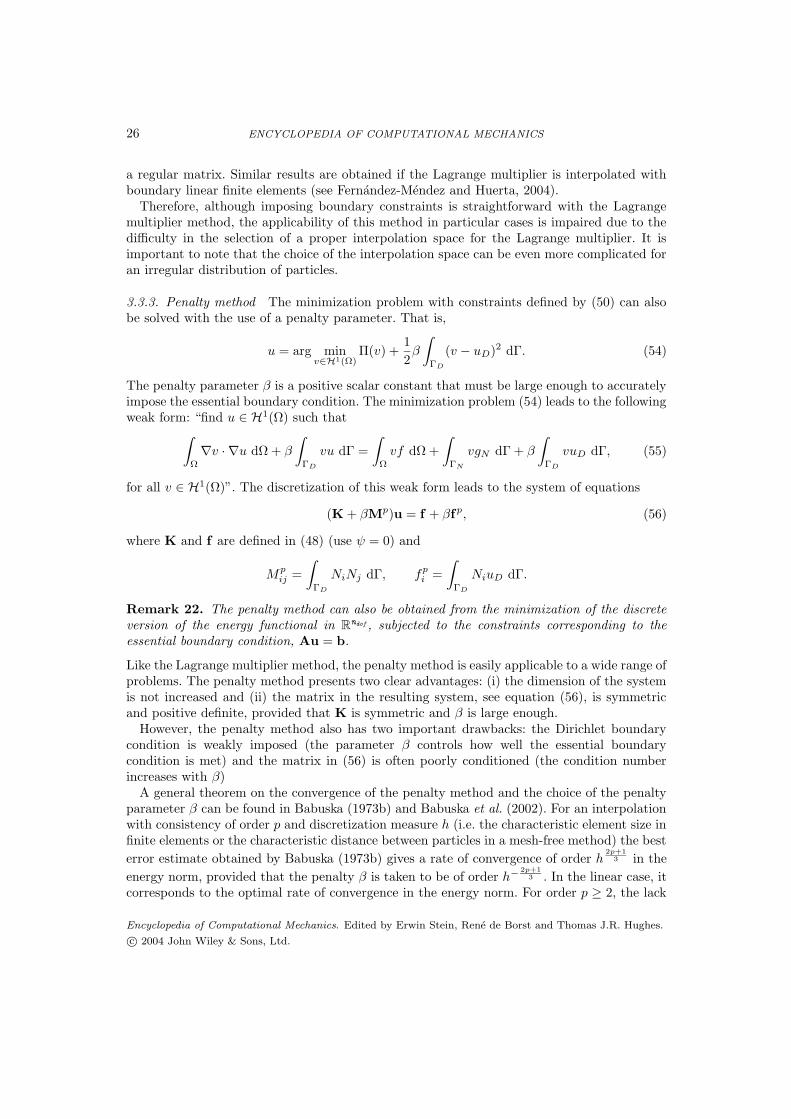
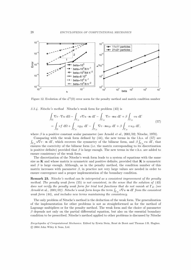
parameter must be large enough, β ≥ 103, in order to impose the boundary condition inan accurate manner. Figure 12 shows convergence curves for different choices of the penaltyparameter. The penalty method converges with a rate close to 2 in the L2 norm if the penaltyparameter β is proportional to h−2. If the penalty parameter is constant, or proportional toh−1, the boundary error dominates and the optimal convergence rate is lost as h goes to zero.
Figure 12 also shows the matrix condition number for increasing values of the penaltyparameter, for a distribution of 11 × 11 and 21 × 21 particles. The condition number growslinearly with the penalty parameter. Note that, for instance, for a discretization with 21 × 21a reasonable value for the penalty parameter is β = 106 which corresponds to a conditionnumber near 1012. Obviously, the situation gets worse for denser discretizations, which needlarger penalty parameters. The ill-conditioning of the matrix reduces the applicability of thepenalty method.
Encyclopedia of Computational Mechanics. Edited by Erwin Stein, Rene de Borst and Thomas J.R. Hughes.
c© 2004 John Wiley & Sons, Ltd.
28 ENCYCLOPEDIA OF COMPUTATIONAL MECHANICS
10−2 10−110
−7
10−6
10−5
10−4
10−3
h
Err
or
1
2
beta=103
beta=103/8 h−1
beta=103/64 h−2
beta=8 104
beta=104 h−1
beta=104/8 h−2
103
104
105
106
107
106
108
1010
1012
1014
k 2
beta
11x11 particles21x21 particles
Figure 12. Evolution of the L2(Ω) error norm for the penalty method and matrix condition number
3.3.4. Nitsche’s method Nitsche’s weak form for problem (43) is∫
Ω
∇v · ∇u dΩ −∫
ΓD
v∇u · n dΓ −∫
ΓD
∇v · nu dΓ + β
∫
ΓD
vu dΓ
=
∫
Ω
vf dΩ +
∫
ΓN
vgN dΓ −∫
ΓD
∇v · nuD dΓ + β
∫
ΓD
v uD dΓ,
(57)
where β is a positive constant scalar parameter (see Arnold et al., 2001/02; Nitsche, 1970).Comparing with the weak form defined by (44), the new terms in the l.h.s. of (57) are∫
ΓDu∇v · n dΓ, which recovers the symmetry of the bilinear form, and β
∫ΓD
vu dΓ, that
ensures the coercivity of the bilinear form (i.e. the matrix corresponding to its discretizationis positive definite) provided that β is large enough. The new terms in the r.h.s. are added toensure consistency of the weak form.
The discretization of the Nitsche’s weak form leads to a system of equations with the samesize as K and whose matrix is symmetric and positive definite, provided that K is symmetricand β is large enough. Although, as in the penalty method, the condition number of thismatrix increases with parameter β, in practice not very large values are needed in order toensure convergence and a proper implementation of the boundary condition.
Remark 23. Nitsche’s method can be interpreted as a consistent improvement of the penaltymethod. The penalty weak form (55) is not consistent, in the sense that the solution of (43)does not verify the penalty weak form for trial test functions that do not vanish at ΓD (seeArnold et al., 2001/02). Nitsche’s weak form keeps the term
∫ΓD
v∇u·n dΓ from the consistent
weak form (44), and includes new terms maintaining the consistency.
The only problem of Nitsche’s method is the deduction of the weak form. The generalizationof the implementation for other problems is not as straightforward as for the method ofLagrange multipliers or for the penalty method. The weak form and the choice of parameterβ depends not only on the partial differential equation, but also on the essential boundarycondition to be prescribed. Nitsche’s method applied to other problems is discussed by Nitsche
Encyclopedia of Computational Mechanics. Edited by Erwin Stein, Rene de Borst and Thomas J.R. Hughes.
c© 2004 John Wiley & Sons, Ltd.

ECM005 29
1
0. 8
1 0 0
1
0. 8
1 0 0
Figure 13. Nitsche’s solution, 7 × 7 distribution of particles, for β = 100 (left) and β = 104 (right)
(1970), by Becker (2002) for the Navier-Stokes problem, by Freud and Stenberg (1995) for theStokes problem, by Hansbo and Larson (2002) for elasticity problems.
Regarding the choice of the parameter, Nitsche proved that if β is taken as β = α/h,where α is a large enough constant and h denotes the characteristic discretization measure,then the discrete solution converges to the exact solution with optimal order in H1 and L2
norms. Moreover, for model problem (43) with Dirichlet boundary conditions, ΓD = ∂Ω, avalue for constant α can be determined taking into account that convergence is ensured ifβ > 2C2, where C is a positive constant such that ‖∇v · n‖L2(∂Ω) ≤ C‖∇v‖L2(Ω) for all v inthe chosen interpolation space. This condition ensures the coercivity of the bilinear form inthe interpolation space. Griebel and Schweitzer (2002) propose the estimation of the constantC as the maximum eigenvalue of the generalized eigenvalue problem,
Av = λBv, (58)
where
Aij =
∫
∂Ω
(∇Ni · n)(∇Nj · n) dΓ, Bij =
∫
Ω
∇Ni · ∇Nj dΩ.
The problem described in Figure 9 can be solved by Nitsche’s method for different valuesof β, see Figure 13. Note that the modification of the weak form is not trivial in this case,see Fernandez-Mendez and Huerta (2004). The major advantage of Nitsche’s method is thatscalar parameter β need not be as large as in the penalty method, and avoids to meet the LBBcondition for the interpolation space for the Lagrange multiplier.
3.4. Incompressibility and volumetric locking in mesh-free methods
Locking in finite elements has been a major concern since its early developments. It appearsbecause poor numerical interpolation leads to an over-constrained system. Locking of standardfinite elements has been extensively studied. It is well known that bilinear finite elementslock in some problems and that biquadratic elements have a better behavior (Hughes, 2000).Moreover, locking has also been studied for increasing polynomial degrees in the context of anhp adaptive strategy, see Suri (1996).
In fact, locking is used in the context of solid mechanics. It is a concern for nearlyincompressible materials. Recall that in plasticity the material is incompressible (Belytschko
Encyclopedia of Computational Mechanics. Edited by Erwin Stein, Rene de Borst and Thomas J.R. Hughes.
c© 2004 John Wiley & Sons, Ltd.

30 ENCYCLOPEDIA OF COMPUTATIONAL MECHANICS
et al., 2000). For instance, let’s consider a linear elastic isotropic material under plane strainconditions and small deformations, namely ∇
su, where u is the displacement and ∇s the
symmetric gradient, i.e. ∇s = 1
2
(∇
T +∇). Dirichlet boundary conditions are imposed on ΓD,
a traction h is prescribed along the Neumann boundary ΓN and there is a body force f . Thus,the problem that needs to be solved may be stated as: solve for u ∈ [H1
ΓD]2 such that
E
1 + ν
∫
Ω
∇sv : ∇
su dΩ +Eν
(1 + ν)(1 − 2ν)
∫
Ω
(∇ · v) (∇ · u) dΩ
=
∫
Ω
f · v dΩ +
∫
ΓN
h · v dΓ ∀v ∈ [H10,ΓD
]2. (59)
In this equation, the standard vector subspaces of H1 are employed for the solution u,[H1
ΓD]2 :=
u ∈ [H1]2 | u = uD on ΓD
(Dirichlet conditions, uD, are automatically satisfied)
and for the test functions v, [H10,ΓD
]2 :=v ∈ [H1]2 | v = 0 on ΓD
, (zero values are imposed
along ΓD).This equation, as discussed by Suri (1996), shows the inherent difficulties of the
incompressible limit. The standard a priori error estimate emanating from (59) and basedon the energy norm may become unbounded for values of ν close to 0.5. In fact, in orderto have finite values of the energy norm the divergence-free condition must be enforced inthe continuum case, i.e. ∇ · u = 0 for u ∈ [H1
ΓD]2, and also in the finite approximation
dimensional space. In fact, locking will occur when the approximation space is not rich enoughfor the approximation to verify the divergence-free condition.
In fluids, the incompressibility is directly the concern. Accurate and efficient modelling ofincompressible flows is an important issue in finite elements. The continuity equation for anincompressible fluid takes a peculiar form. It consists of a constraint on the velocity field whichmust be divergence free. Then, the pressure has to be considered as a variable not related to anyconstitutive equation. Its presence in the momentum equation has the purpose of introducingan additional degree of freedom needed to satisfy the incompressibility constraint. The role ofthe pressure variable is thus to adjust itself instantaneously in order to satisfy the conditionof divergence-free velocity. That is, the pressure is acting as a Lagrange multiplier of theincompressibility constraint and thus there is a coupling between the velocity and the pressureunknowns.
Various formulations have been proposed for incompressible flow (Girault and Raviart, 1986;Gresho and Sani, 2000; Gunzburger, 1989; Pironneau, 1989; Quartapelle, 1993; Quarteroni andValli, 1994; Temam, 2001; Donea and Huerta, 2003). Mixed finite elements present numericaldifficulties caused by the saddle-point nature of the resulting variational problem. Solvabilityof the problem depends on a proper choice of finite element spaces for velocity and pressure.They must satisfy a compatibility condition, the so-called LBB (or inf-sup) condition. If thisis not the case, alternative formulations (usually depending on a numerical parameter) aredevised to circumvent the LBB condition and enable the use of velocity–pressure pairs thatare unstable in the standard Galerkin formulation.
Incompressibility in mesh-free methods is still an open topic. Even recently, it was claimed(Zhu and Atluri, 1998) that meshless methods do not exhibit volumetric locking. Now it isclear that this is not true, as shown in a study of the element free Galerkin (EFG) method byDolbow and Belytschko (1999). Moreover, several authors claim that increasing the dilationparameter locking phenomena in mesh-free methods can be suppressed, or at least attenuated
Encyclopedia of Computational Mechanics. Edited by Erwin Stein, Rene de Borst and Thomas J.R. Hughes.
c© 2004 John Wiley & Sons, Ltd.

ECM005 31
(Askes et al., 1999; Dolbow and Belytschko, 1999; Chen et al., 2000). Huerta and Fernandez-Mendez (2001) clarify this issue and determine the influence of the dilation parameter onthe locking behavior of EFG near the incompressible limit by a modal analysis. The majorconclusions are:1.- The number of non-physical locking modes is independent of the ratio ρ/h.2.- An increase of the dilation parameter decreases the eigenvalue (amount of energy) in
the locking mode and attenuates, but does not suppress volumetric locking (in theincompressible limit the energy will remain unbounded).
3.- An increase in the order of consistency decreases the number of non-physical locking modes.4.- The decrease in the number of non-physical locking modes is slower than in finite elements.
Thus EFG will not improve the properties of the FEM (from a volumetric lockingviewpoint) for p or h-p refinement. However, for practical purposes and as in finiteelements, in EFG an h-p strategy will also suppress locking.
The remedies proposed in the literature are, in general, extensions of the methods developedfor finite elements. For instance, Dolbow and Belytschko (1999) propose an EFG formulationusing selective reduced integration. Chen et al. (2000) suggest an improved RKPM based on apressure projection method. These alternatives have the same advantages and inconveniencesas in standard finite element methods. Perhaps it is worth noting that in mesh-free methodsit is non trivial to verify analytically the LBB condition for a given interpolation of velocityand pressure.
One alternative that uses the inherent properties of mesh-free methods and does not havea parallel in finite elements is the pseudo-divergence-free approach (Vidal et al., 2002; Huertaet al., 2004a). This method is based on diffuse derivatives (see Section 2.2.6) which convergeto the derivatives of the exact solution when the radius of the support, ρ, goes to zero (for afixed ratio ρ/h). One of the key advantages of this approach is that the expressions of pseudo-divergence-free interpolation functions are computed a priori. That is, prior to determiningthe specific particle distribution. Thus, there is no extra computational cost because only theinterpolating polynomials are modified compared with standard EFG.
4. RADIAL BASIS FUNCTIONS
Radial basis functions (RBF) have been studied in mathematics for the past 30 years and areclosely related to mesh-free approximations. There are two major differences in between thecurrent practice approaches in radial basis functions and those described in previous Sections:
1. Most radial basis functions have non compact support.2. Completeness is provided by adding a global polynomial to the basis.
For these two reasons, the solution procedures usually have to be tailored for this class ofglobal interpolants. Two techniques that avoid the drawbacks of global approximations are
1. Multipolar methods2. Domain decomposition techniques
The most commonly used radial basis functions (with their names) are
Encyclopedia of Computational Mechanics. Edited by Erwin Stein, Rene de Borst and Thomas J.R. Hughes.
c© 2004 John Wiley & Sons, Ltd.
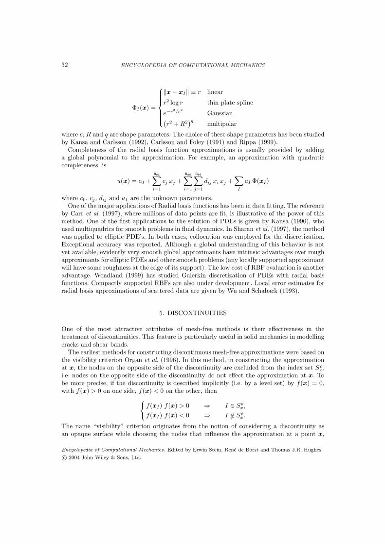
32 ENCYCLOPEDIA OF COMPUTATIONAL MECHANICS
ΦI(x) =
‖x − xI‖ ≡ r linear
r2 log r thin plate spline
e−r2/c2
Gaussian(r2 +R2
)qmultipolar
where c, R and q are shape parameters. The choice of these shape parameters has been studiedby Kansa and Carlsson (1992), Carlsson and Foley (1991) and Rippa (1999).
Completeness of the radial basis function approximations is usually provided by addinga global polynomial to the approximation. For example, an approximation with quadraticcompleteness, is
u(x) = c0 +
nsd∑
i=1
cj xj +
nsd∑
i=1
nsd∑
j=1
dij xi xj +∑
I
aI Φ(xI)
where c0, cj , dij and aI are the unknown parameters.One of the major applications of Radial basis functions has been in data fitting. The reference
by Carr et al. (1997), where millions of data points are fit, is illustrative of the power of thismethod. One of the first applications to the solution of PDEs is given by Kansa (1990), whoused multiquadrics for smooth problems in fluid dynamics. In Sharan et al. (1997), the methodwas applied to elliptic PDE’s. In both cases, collocation was employed for the discretization.Exceptional accuracy was reported. Although a global understanding of this behavior is notyet available, evidently very smooth global approximants have intrinsic advantages over roughapproximants for elliptic PDEs and other smooth problems (any locally supported approximantwill have some roughness at the edge of its support). The low cost of RBF evaluation is anotheradvantage. Wendland (1999) has studied Galerkin discretization of PDEs with radial basisfunctions. Compactly supported RBFs are also under development. Local error estimates forradial basis approximations of scattered data are given by Wu and Schaback (1993).
5. DISCONTINUITIES
One of the most attractive attributes of mesh-free methods is their effectiveness in thetreatment of discontinuities. This feature is particularly useful in solid mechanics in modellingcracks and shear bands.
The earliest methods for constructing discontinuous mesh-free approximations were based onthe visibility criterion Organ et al. (1996). In this method, in constructing the approximationat x, the nodes on the opposite side of the discontinuity are excluded from the index set Sρ
x,i.e. nodes on the opposite side of the discontinuity do not effect the approximation at x. Tobe more precise, if the discontinuity is described implicitly (i.e. by a level set) by f(x) = 0,with f(x) > 0 on one side, f(x) < 0 on the other, then
f(xI) f(x) > 0 ⇒ I ∈ Sρ
x,
f(xI) f(x) < 0 ⇒ I 6∈ Sρx.
The name “visibility” criterion originates from the notion of considering a discontinuity asan opaque surface while choosing the nodes that influence the approximation at a point x,
Encyclopedia of Computational Mechanics. Edited by Erwin Stein, Rene de Borst and Thomas J.R. Hughes.
c© 2004 John Wiley & Sons, Ltd.

ECM005 33
discontinuityf=0
f>0
f<0
f>0
f<0
r θ
crack
a) b)
Figure 14. a) level set describing discontinuity, b) nomenclature for cracktip branch functions
namely Sρx. If a node xI is invisible from x, then node I is not included in the index set Sρ
x
even when it falls within the domain of influence.When a discontinuity ends within a domain, such as at a cracktip, the visibility criterion
does not provide an adequate tool for constructing the discontinuity in the approximation.Around the cracktip the approximation must be constructed so that it is continuous in frontof the cracktip, but discontinuous behind it. One way to accomplish this is to include in thebasis branch functions of the form
BiI = [r2 sinθ
2, r2 sin
θ
2] (60)
where θ is the angle between the line to the cracktip and the tangent to the crack and r is thedistance to the cracktip, see Fig. 14b.
For cracks in elastic materials, the basis can be enriched by branch functions that span theasymptotic neartip field of the Westergard solution, see Fleming et al. (1997). The basis isthen the polynomial basis plus the functions
BiI = [√r sin
θ
2,√r sin
θ
2sin θ,
√r cos
θ
2,√r cos
θ
2cos θ] (61)
Since this basis includes the first order terms in the neartip field solution, very accuratesolutions can be obtained with coarse discretizations. Xiao and Karihaloo (2003) have shownthat even better accuracy can be attained by adding higher order terms in the asymptoticfield. The idea of incorporating special functions can also be found, among others, in Odenand Duarte (1997).
Regardless of whether a branch function is used near the cracktip, if the visibility criterionis used for constructing the approximation near the end of the discontinuity, additionaldiscontinuities may occur around the tip. Two such discontinuities are shown in Fig. 15. Theycan be avoided if the visibility criterion is not used near the tip. Krysl and Belytschko (1997)have shown that these discontinuities do not impair the convergence of the solution since their
Encyclopedia of Computational Mechanics. Edited by Erwin Stein, Rene de Borst and Thomas J.R. Hughes.
c© 2004 John Wiley & Sons, Ltd.
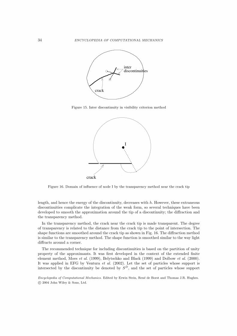
34 ENCYCLOPEDIA OF COMPUTATIONAL MECHANICS
crack
interdiscontinuities
Figure 15. Inter discontinuity in visibility criterion method
I
crack
Figure 16. Domain of influence of node I by the transparency method near the crack tip
length, and hence the energy of the discontinuity, decreases with h. However, these extraneousdiscontinuities complicate the integration of the weak form, so several techniques have beendeveloped to smooth the approximation around the tip of a discontinuity; the diffraction andthe transparency method.
In the transparency method, the crack near the crack tip is made transparent. The degreeof transparency is related to the distance from the crack tip to the point of intersection. Theshape functions are smoothed around the crack tip as shown in Fig. 16. The diffraction methodis similar to the transparency method. The shape function is smoothed similar to the way lightdiffracts around a corner.
The recommended technique for including discontinuities is based on the partition of unityproperty of the approximants. It was first developed in the context of the extended finiteelement method, Moes et al. (1999), Belytschko and Black (1999) and Dolbow et al. (2000).It was applied in EFG by Ventura et al. (2002). Let the set of particles whose support isintersected by the discontinuity be denoted by SD, and the set of particles whose support
Encyclopedia of Computational Mechanics. Edited by Erwin Stein, Rene de Borst and Thomas J.R. Hughes.
c© 2004 John Wiley & Sons, Ltd.

ECM005 35
a) b)
II
PSfrag replacements
f1(x) = 0 f1(x) = 0
f2(x) = 0 f2(x) = 0
Figure 17. a) Support of node I with a) intersecting discontinuities and b) branching discontinuities
includes the tip of the discontinuity be ST . The approximation is then given by
uh(x) =∑
I∈Sρx
NI(x) uI +∑
I∈SD∩Sρx
NI(x) H(f(x)
)q
(1)I +
∑
I∈ST ∩Sρx
NI(x)∑
J
(BJ · q(2)
J
),
where H(·) is the step function (Heaviside function). It is easy to show that the weak form(see Belytschko and Black, 1999) then yields the requisite strong form for elastic problems;this is probably also true for partial differential equations describing other physical problems.
The technique can also be used for intersecting and branching discontinuities, see Daux etal. (2000) and Belytschko et al. (2001). For example, consider the geometry shown in Fig. 17.Let J1 be the set of nodes whose domains of influence include the discontinuity f1(x) = 0, J2
the corresponding set for f2(x) = 0. Let J3 = J1 ∩ J2. Then the approximation is
uh(x) =∑
I∈Sρx
NI(x) uI +∑
I∈J1∩Sρx
NI(x) H(f1(x)
)q
(1)I
+∑
I∈J2∩Sρx
NI(x) H(f2(x)
)q
(2)I +
∑
I∈J3∩Sρx
NI(x) H(f1(x)
)H
(f2(x)
)q
(3)I .
5.1. Discontinuities in gradients
The continuously differentiable character of mesh-free approximation functions is sometimesa disadvantage. At material interfaces in continua, or more generally, at discontinuities of thecoefficients of a PDE, solutions of elliptic and parabolic systems have discontinuous gradients.These discontinuities in the gradient need to be explicitly incorporated in mesh-free methods.
One of the first treatments of discontinuous gradients was by Cordes and Moran (1996).They treated the construction of the approximation separately; that is, they subdivided thedomain into two subdomains. Let the subdomains Ω1 and Ω2 be with interface Γint. Theyenforced continuity of the function along Γint by Lagrange multipliers. Since the approximationu(Ω1) was constructed without considering any nodes in Ω2, and vice versa, the gradient of
Encyclopedia of Computational Mechanics. Edited by Erwin Stein, Rene de Borst and Thomas J.R. Hughes.
c© 2004 John Wiley & Sons, Ltd.

36 ENCYCLOPEDIA OF COMPUTATIONAL MECHANICS
the approximation will be discontinuous across Γint after the continuity of the approximationis enforced by Lagrange multipliers. As in the case of essential boundary conditions, thiscontinuity of the function can also be enforced by penalty methods, augmented Lagrangianmethods or Nitsche’s method.
An alternative technique was proposed by Krongauz and Belytschko (1998a), who added afunction with a discontinuous gradient. In the original paper, the approximation is enrichedwith the absolute values of a signed distance function.
This enrichment function can also be employed with a local or global partition of unity
uh = Ni ui +Ni |f(x)| qiThis was first studied in a finite element context by Sukumar et al. (2001) and Belytschko etal. (2001). In a finite element, the local partition of unity has some difficulties because theenrichment function does not decay, so it is difficult to fade it out gracefully. A global partitionof unity is also undesirable. This behavior of this enrichment in mesh-free methods has notbeen studied.
The local partition of unity method can also be used for intersecting gradient discontinuities,branching gradient discontinuities and unclosed gradient discontinuities. The techniques areidentical to those for discontinuities in functions, except that the step function is replacedby the absolute values of the signed distance function. For example, the approximation for afunction with the intersecting discontinuities shown in Fig. 17a is given by
uh(x) =∑
I∈Sρx
NI(x) uI +∑
I∈J1∩Sρx
NI(x) |f1(x)| q(1)I
+∑
I∈J2∩Sρx
NI(x) |f2(x)| q(2)I +
∑
I∈J3∩Sρx
NI(x) |f1(x)| |f2(x)| q(3)I .
The enrichment procedures are substantially simpler to implement than the domainsubdivision/constraint technique of Cordes and Moran (1996), particularly for complexpatterns such as intersecting and branching gradient discontinuities.
6. BLENDING MESH-FREE METHODS AND FINITE ELEMENTS
Several authors have proposed different alternatives to blend finite elements and mesh-freemethods. These approximations are combined for two purposes: either i) to couple bothinterpolations, or ii) to enrich the finite element interpolation using particles.
In the first scenario, the objective is to benefit from the advantages of each interpolationin different regions of the computational domain, which is usually divided in three regions,see Figure 18. In one region only finite elements are present, another with only mesh-freeapproximation functions, and a transition region.
In the second case, the enrichment improves the approximation without remeshing. A finiteelement interpolation is considered in the whole domain and particles can be added in orderto improve the interpolation in a selected region.
Coupled finite elements/mesh-free methods are proposed by Belytschko et al. (1995). Theyshow how to couple finite elements near the Dirichlet boundaries and EFG in the interior of
Encyclopedia of Computational Mechanics. Edited by Erwin Stein, Rene de Borst and Thomas J.R. Hughes.
c© 2004 John Wiley & Sons, Ltd.
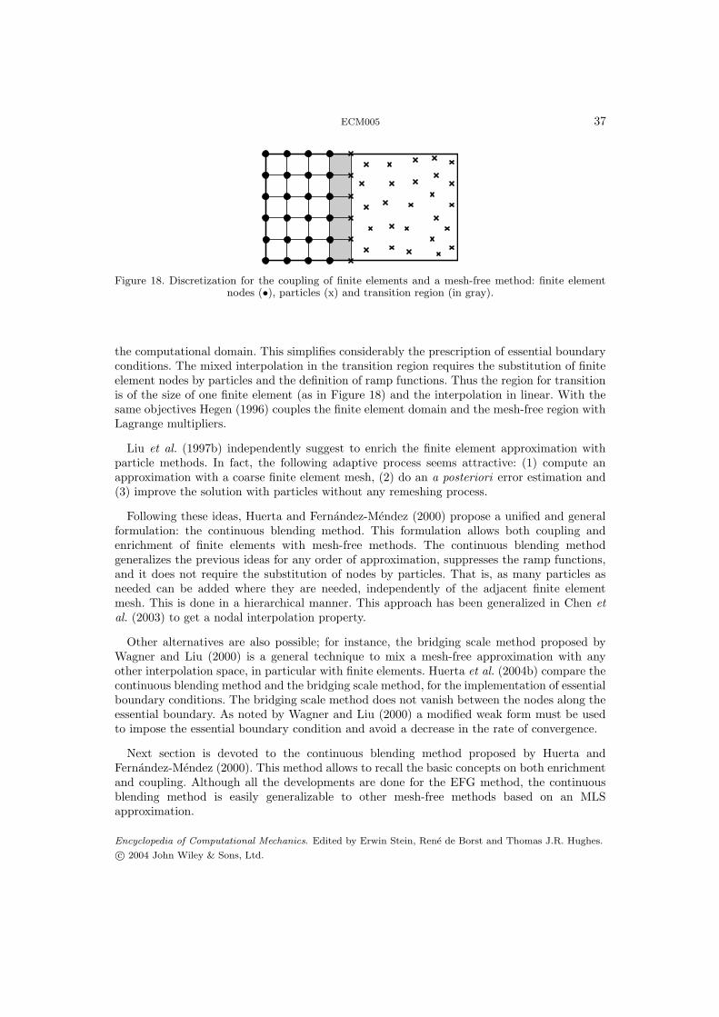
ECM005 37
Figure 18. Discretization for the coupling of finite elements and a mesh-free method: finite elementnodes (•), particles (x) and transition region (in gray).
the computational domain. This simplifies considerably the prescription of essential boundaryconditions. The mixed interpolation in the transition region requires the substitution of finiteelement nodes by particles and the definition of ramp functions. Thus the region for transitionis of the size of one finite element (as in Figure 18) and the interpolation in linear. With thesame objectives Hegen (1996) couples the finite element domain and the mesh-free region withLagrange multipliers.
Liu et al. (1997b) independently suggest to enrich the finite element approximation withparticle methods. In fact, the following adaptive process seems attractive: (1) compute anapproximation with a coarse finite element mesh, (2) do an a posteriori error estimation and(3) improve the solution with particles without any remeshing process.
Following these ideas, Huerta and Fernandez-Mendez (2000) propose a unified and generalformulation: the continuous blending method. This formulation allows both coupling andenrichment of finite elements with mesh-free methods. The continuous blending methodgeneralizes the previous ideas for any order of approximation, suppresses the ramp functions,and it does not require the substitution of nodes by particles. That is, as many particles asneeded can be added where they are needed, independently of the adjacent finite elementmesh. This is done in a hierarchical manner. This approach has been generalized in Chen etal. (2003) to get a nodal interpolation property.
Other alternatives are also possible; for instance, the bridging scale method proposed byWagner and Liu (2000) is a general technique to mix a mesh-free approximation with anyother interpolation space, in particular with finite elements. Huerta et al. (2004b) compare thecontinuous blending method and the bridging scale method, for the implementation of essentialboundary conditions. The bridging scale method does not vanish between the nodes along theessential boundary. As noted by Wagner and Liu (2000) a modified weak form must be usedto impose the essential boundary condition and avoid a decrease in the rate of convergence.
Next section is devoted to the continuous blending method proposed by Huerta andFernandez-Mendez (2000). This method allows to recall the basic concepts on both enrichmentand coupling. Although all the developments are done for the EFG method, the continuousblending method is easily generalizable to other mesh-free methods based on an MLSapproximation.
Encyclopedia of Computational Mechanics. Edited by Erwin Stein, Rene de Borst and Thomas J.R. Hughes.
c© 2004 John Wiley & Sons, Ltd.
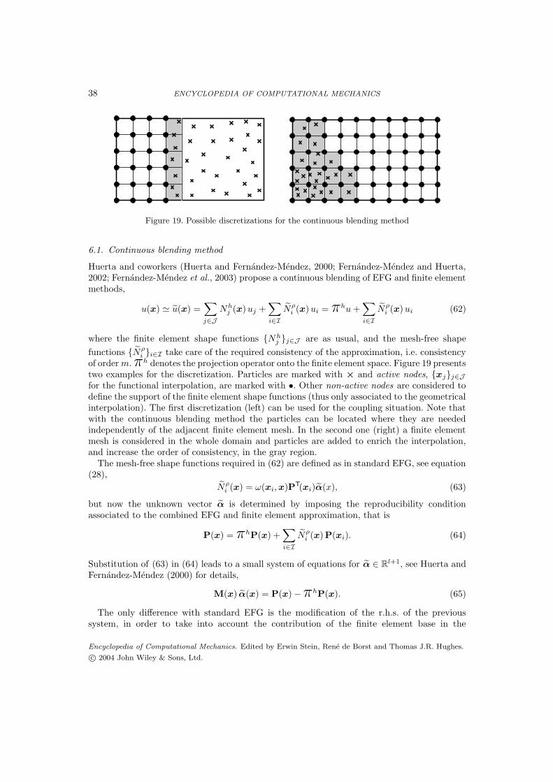
38 ENCYCLOPEDIA OF COMPUTATIONAL MECHANICS
Figure 19. Possible discretizations for the continuous blending method
6.1. Continuous blending method
Huerta and coworkers (Huerta and Fernandez-Mendez, 2000; Fernandez-Mendez and Huerta,2002; Fernandez-Mendez et al., 2003) propose a continuous blending of EFG and finite elementmethods,
u(x) ' u(x) =∑
j∈J
Nhj (x)uj +
∑
i∈I
Nρi (x)ui = π
hu+∑
i∈I
Nρi (x)ui (62)
where the finite element shape functions Nhj j∈J are as usual, and the mesh-free shape
functions Nρi i∈I take care of the required consistency of the approximation, i.e. consistency
of orderm.πh denotes the projection operator onto the finite element space. Figure 19 presentstwo examples for the discretization. Particles are marked with × and active nodes, xjj∈J
for the functional interpolation, are marked with •. Other non-active nodes are considered todefine the support of the finite element shape functions (thus only associated to the geometricalinterpolation). The first discretization (left) can be used for the coupling situation. Note thatwith the continuous blending method the particles can be located where they are neededindependently of the adjacent finite element mesh. In the second one (right) a finite elementmesh is considered in the whole domain and particles are added to enrich the interpolation,and increase the order of consistency, in the gray region.
The mesh-free shape functions required in (62) are defined as in standard EFG, see equation(28),
Nρi (x) = ω(xi,x)PT(xi)α(x), (63)
but now the unknown vector α is determined by imposing the reproducibility conditionassociated to the combined EFG and finite element approximation, that is
P(x) = πhP(x) +
∑
i∈I
Nρi (x)P(xi). (64)
Substitution of (63) in (64) leads to a small system of equations for α ∈ Rl+1, see Huerta andFernandez-Mendez (2000) for details,
M(x) α(x) = P(x) −πhP(x). (65)
The only difference with standard EFG is the modification of the r.h.s. of the previoussystem, in order to take into account the contribution of the finite element base in the
Encyclopedia of Computational Mechanics. Edited by Erwin Stein, Rene de Borst and Thomas J.R. Hughes.
c© 2004 John Wiley & Sons, Ltd.

ECM005 39
approximation. Moreover, note that the expression for the modified EFG shape functions isindependent of the situation, i.e the same implementation is valid for enrichment and coupling,increasing the versatility of this approach.
Figure 20. Shape functions of the coupled finite element (solid line) and mesh-free (dashed line)interpolation.
Figure 20 shows a 1D example coupling finite elements and EFG. The mesh-free shapefunctions adapt their shape to recover the linear interpolation. In the coupling situation thecontinuity of the interpolation is ensured under some conditions, even in multiple dimensions,by the following result, see Fernandez-Mendez and Huerta (2002; 2004) for the proof.
Proposition 3. The approximation u(x), defined in (62), is continuous in Ω if: (1.-) thesame order of consistency, m, is imposed all over Ω (i.e. m coincides with the degree of theFE base), and (2.-) the domain of influence of particles coincides exactly with the region wherefinite elements do not have a complete basis.
Remark 24 (Imposing Dirichlet boundary conditions) Under the assumptions (1.-)and (2.-) in Proposition 3, the contribution of the particles is zero in the regions where
the finite element base is complete. In particular, this means that Nρi = 0 in the finite element
edges (or faces in 3D) whose nodes are all in J (active nodes). This is an important propertyfor the implementation of essential boundary conditions. If a finite element mesh with activenodes at the essential boundary is used, the mesh-free shape functions take care of reproducingpolynomials up to degree m in Ω and, at the same time, vanish at the essential boundary. Forinstance, Figure 21 shows the particle shape functions, Nρ
i = 0, associated to particles at theboundary and in the first interior layer. Note that they vanish along the boundary because thefinite element base is complete on ∂Ω. Therefore, the prescribed values can be directly imposedas usual in the framework of finite elements, by setting the values of the corresponding nodalcoefficients. Moreover, it is also easy to impose that the test functions (for the weak forms)vanish along the Dirichlet boundary, see Fernandez-Mendez and Huerta (2004) for furtherdetails.
The problem described in Figure 9 can be solved using the continuous blending method,Figure 22 shows the solution. As observed in Remark 24, the prescribed displacements aredirectly imposed. Two different finite element discretizations are considered. In both cases,the linear finite element approximation at the boundary, allows the exact enforcement ofthe prescribed displacement. Note that if the prescribed displacement is piecewise linear orpiecewise constant, as it is in this example, then it is imposed exactly when a bilinear finiteelement approximation is used.
Finally, an example reproduces the finite element enrichment with EFG in a nonlinearcomputational problem. A rectangular specimen with an imperfection is loaded (see Dıez et
Encyclopedia of Computational Mechanics. Edited by Erwin Stein, Rene de Borst and Thomas J.R. Hughes.
c© 2004 John Wiley & Sons, Ltd.
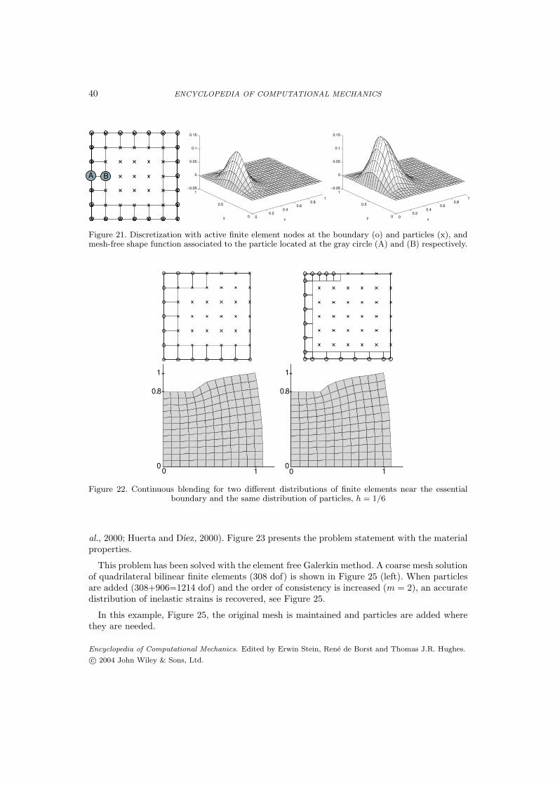
40 ENCYCLOPEDIA OF COMPUTATIONAL MECHANICS
A B
00.2
0.40.6
0.81
0
0.5
1−0.05
0
0.05
0.1
0.15
xy 00.2
0.40.6
0.81
0
0.5
1−0.05
0
0.05
0.1
0.15
xy
Figure 21. Discretization with active finite element nodes at the boundary (o) and particles (x), andmesh-free shape function associated to the particle located at the gray circle (A) and (B) respectively.
0. 8
1
0 1 0
0. 8
1
0 1 0
Figure 22. Continuous blending for two different distributions of finite elements near the essentialboundary and the same distribution of particles, h = 1/6
al., 2000; Huerta and Dıez, 2000). Figure 23 presents the problem statement with the materialproperties.
This problem has been solved with the element free Galerkin method. A coarse mesh solutionof quadrilateral bilinear finite elements (308 dof) is shown in Figure 25 (left). When particlesare added (308+906=1214 dof) and the order of consistency is increased (m = 2), an accuratedistribution of inelastic strains is recovered, see Figure 25.
In this example, Figure 25, the original mesh is maintained and particles are added wherethey are needed.
Encyclopedia of Computational Mechanics. Edited by Erwin Stein, Rene de Borst and Thomas J.R. Hughes.
c© 2004 John Wiley & Sons, Ltd.
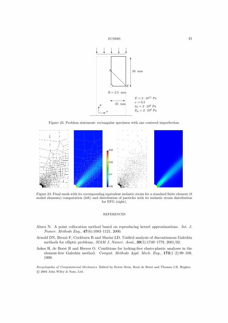
ECM005 41
@@
@@
A′
A
? ? ? ? ?
?
6
-
50 mm
25 mm
R = 2.5 mm
E = 2 · 1011 Pa
ν = 0.3
σ0 = 2 · 108 Pa
Ep = 2 · 108 Pa-6
x
y
Figure 23. Problem statement: rectangular specimen with one centered imperfection.
Deformacion plastica equivalente final
VAL − ISO
> 0.00E+00
< 4.14E−02
0.00E+00
2.00E−03
4.00E−03
6.00E−03
8.00E−03
1.00E−02
1.20E−02
1.40E−02
1.60E−02
1.80E−02
2.00E−02
2.20E−02
2.40E−02
2.60E−02
2.80E−02
3.00E−02
Figure 24. Final mesh with its corresponding equivalent inelastic strain for a standard finite element (8noded elements) computation (left) and distribution of particles with its inelastic strain distribution
for EFG (right).
REFERENCES
Aluru N. A point collocation method based on reproducing kernel approximations. Int. J.Numer. Methods Eng., 47(6):1083–1121, 2000.
Arnold DN, Brezzi F, Cockburn B and Marini LD. Unified analysis of discontinuous Galerkinmethods for elliptic problems. SIAM J. Numer. Anal., 39(5):1749–1779, 2001/02.
Askes H, de Borst R and Heeres O. Conditions for locking-free elasto-plastic analyses in theelement-free Galerkin method. Comput. Methods Appl. Mech. Eng., 173(1–2):99–109,1999.
Encyclopedia of Computational Mechanics. Edited by Erwin Stein, Rene de Borst and Thomas J.R. Hughes.
c© 2004 John Wiley & Sons, Ltd.

42 ENCYCLOPEDIA OF COMPUTATIONAL MECHANICS
Figure 25. Coarse finite element mesh (Q1 elements) with its corresponding equivalent inelastic strain(right) and mixed interpolation with its equivalent inelastic strain distribution (left).
Babuska I and Melenk J. The partition of the unity finite element method. TechnicalReport BN-1185, Institute for Physical Science and Technology, University of Maryland,Maryland, 1995.
Babuska I, Banerjee U and Osborn JE. Meshless and generalized finite element methods:A survey of some major results. In Griebel M and Schweitzer MA, editors, Meshfreemethods for partial differential equations, volume 26 of Lecture Notes in ComputationalScience and Engineering, pages 1–20. Springer-Verlag, Berlin, 2002.
Babuska I. The finite element method with lagrange multipliers. Numer. Math., 20:179–192,1973.
Babuska I. The finite element method with penalty. Math. Comp., 27:221–228, 1973.
Becker R. Mesh adaptation for dirichlet flow control via Nitsche’s method. Commun. Numer.Methods Eng., 18(9):669–680, 2002.
Belytschko T and Black T. Elastic crack growth in finite elements with minimal remeshing.Int. J. Numer. Methods Eng., 45(5):601–620, 1999.
Belytschko T and Organ D. Element-free Galerkin methods for dynamic fracture in concrete.In D.R.J. Owen EO and Hilton E, editors, Computational Plasticity. Fundamentals andApplications, pages 304–321, Barcelona, Spain, 1997.
Belytschko T, Lu YY and Gu L. Element free Galerkin methods. Int. J. Numer. MethodsEng., 37(2):229–256, 1994.
Belytschko T, Organ D and Krongauz Y. A coupled finite element–element-free Galerkinmethod. Comput. Mech., 17(3):186–195, 1995.
Belytschko T, Krongauz Y, Organ D, Fleming M and Krysl P. Meshless methods: an overviewand recent developments. Comput. Methods Appl. Mech. Eng., 139(1–4):3–47, 1996.
Belytschko T, Krongauz Y, Fleming M, Organ D and Liu WK. Smoothing and acceleratedcomputations in the element free Galerkin method. J. Comput. Appl. Math., 74(1–2):111–126, 1996.
Encyclopedia of Computational Mechanics. Edited by Erwin Stein, Rene de Borst and Thomas J.R. Hughes.
c© 2004 John Wiley & Sons, Ltd.

ECM005 43
Belytschko T, Liu WK and Moran B. Nonlinear finite elements for continua and structures.John Wiley & Sons, Chichester, 2000.
Belytschko T, Moes N, Usui S and Parimi C. Arbitrary discontinuities in finite elements. Int.J. Numer. Methods Eng., 50(4):993–1013, 2001.
Bonet J and Kulasegaram S. Correction and stabilization of smooth particle hydrodynamicsmethods with applications in metal forming simulations. Int. J. Numer. Methods Eng.,47(6):1189–1214, 2000.
Bonet J and Lok T. Variational and momentum preservation aspects of smooth particlehydrodynamic formulations. Comput. Methods Appl. Mech. Eng., 180(1-2):97–115, 1999.
Bouillard P and Suleau S. Element-free Galerkin method for helmholtz problems: formulationand numerical assessment of the pollution effect. Comput. Methods Appl. Mech. Eng.,162(1-4):317–335, 1998.
Breitkopf P, Rassineux A and Villon P. Mesh-free operators for consistent field transferin large deformation plasticity. In Book of abstracts of the 2nd European Conferenceon Computational Mechanics: Solids, Structures and Coupled Problems in Engineering,Cracow, Poland, 2001.
Brezzi F. On the existence, uniqueness and approximation of saddle-point problemsarising from Lagrangian multipliers. Rev. Francaise Automat. Informat. RechercheOperationnelle Ser. Rouge, 8(R-2):129–151, 1974.
Carlsson R and Foley T. The parameter r2 in multiquadric interpolation. Computers andMathematics with applications, 21:29–42, 1991.
Carr JC, Fright WR and Beatson RK. Surface interpolation with radial basis functions formedical imaging. IEEE Trans. Med. Imaging, 16(1):96–107, 1997.
Chen JS, Pan C, Wu CT and Liu WK. Reproducing kernel particle methods for largedeformation analysis of non-linear. Comput. Methods Appl. Mech. Eng., 139(1-4):195–227, 1996.
Chen JS, Yoon S, Wang H and Liu WK. An improved reproducing kernel particle method fornearly incompressible finite elasticity. Comput. Methods Appl. Mech. Eng., 181(1–3):117–145, 2000.
Chen JS, Han W, You Y and Meng X. A reproducing kernel method with nodal interpolationproperty. Int. J. Numer. Methods Eng., 56(7):935–960, 2003.
Chu YA and Moran B. A computational model for nucleation of solid-solid phasetransformations. Model. Simul. Mater. Sci. Eng., 3:455–471, 1995.
Cordes LW and Moran B. Treatment of material discontinuity in the element-free Galerkinmethod. Comput. Methods Appl. Mech. Eng., 139(1–4):75–89, 1996.
Daux C, Moes N, Dolbow J, Sukumar N and Belyscthko T. Arbitrary branched andintersecting cracks with the extended finite element method. Int. J. Numer. MethodsEng., 48(12):1741–1760, 2000.
De S and Bathe KJ. The method of finite spheres. Comput. Mech., 25(4):329–345, 2000.
Dıez P, Arroyo M and Huerta A. Adaptivity based on error estimation for viscoplastic softeningmaterials. Mech. Cohesive-Frict. Mater., 5(2):87–112, 2000.
Encyclopedia of Computational Mechanics. Edited by Erwin Stein, Rene de Borst and Thomas J.R. Hughes.
c© 2004 John Wiley & Sons, Ltd.
44 ENCYCLOPEDIA OF COMPUTATIONAL MECHANICS
Dilts G. Moving-least-square-particles-hydrdodynamics I: Consistency and stability. Int. J.Numer. Methods Eng., 44(8):1115–1155, 1999.
Dolbow J and Belytschko T. Volumetric locking in the element free Galerkin method. Int. J.Numer. Methods Eng., 46(6):925–942, 1999.
Dolbow J, Moes N and Belytschko T. Discontinuous enrichment in finite elements with apartition of unity method. Finite Elem. Anal. and Des., 36(3–4):235–260, 2000.
Donea J and Huerta A. Finite element methods for flow problems. John Wiley & Sons,Chichester, 2003.
Duarte CA and Oden JT. h-p clouds – an h-p meshless method. Numer. Methods PartialDiffer. Equations, 12(6):673–705, 1996.
Duarte CA and Oden JT. An h-p adaptive method using clouds. Comput. Methods Appl.Mech. Eng., 139(1-4):237–262, 1996.
Dyka CT. Addressing tension instability in SPH methods. Technical Report NRL/MR/6384,NRL, 1994.
Fernandez-Mendez S and Huerta A. Coupling finite elements and particles for adaptivity: Anapplication to consistently stabilized convection-diffusion. In Griebel M and SchweitzerMA, editors, Meshfree methods for partial differential equations, volume 26 of LectureNotes in Computational Science and Engineering, pages 117–129. Springer-Verlag, Berlin,2002.
Fernandez-Mendez S and Huerta A. Imposing essential boundary conditions in mesh-freemethods. Comput. Methods Appl. Mech. Eng., 193, 2004.
Fernandez-Mendez S, Dıez P and Huerta A. Convergence of finite elements enriched withmeshless methods. Numer. Math., 96(1):43–59, 2003.
Fleming M, Chu YA, Moran B and Belytschko T. Enriched element-free Galerkin methods forcrack tip fields. Int. J. Numer. Methods Eng., 40(8):1483–1504, 1997.
Freud J and Stenberg R. On weakly imposed boundary conditions for second order problems.In Proceeding of the International Conference on Finite Elements in Fluids - New trendsand applications, Venezia, 1995.
Gingold RA and Monaghan JJ. Smoothed particle hydrodynamics: theory and application tonon-spherical stars. Mon. Notices Royal Astro. Soc., 181:375–389, 1977.
Girault V and Raviart PA. Finite element methods for Navier-Stokes equations. Theory andalgorithms. Springer-Verlag, Berlin, 1986.
Gosz J and Liu WK. Admissible approximations for essential boundary conditions in thereproducing kernel particle method. Comput. Mech., 19(2):120–135, 1996.
Gresho PM and Sani RL. Incompressible flow and the finite element method. Vol. 1: Advectiondiffusion. Vol. 2: Isothermal laminar flow. John Wiley & Sons, Chichester, 2000.
Griebel M and Schweitzer MA. A particle-partition of unity method. Part V: Boundaryconditions. In Hildebrandt S and Karcher H, editors, Geometric Analysis and NonlinearPartial Differential Equations, pages 517–540, Berlin, 2002. Springer.
Gunter FC and Liu WK. Implementation of boundary conditions for meshless methods.Comput. Methods Appl. Mech. Eng., 163(1-4):205–230, 1998.
Encyclopedia of Computational Mechanics. Edited by Erwin Stein, Rene de Borst and Thomas J.R. Hughes.
c© 2004 John Wiley & Sons, Ltd.

ECM005 45
Gunzburger MD. Finite element methods for viscous incompressible flows. A guide to theory,practice, and algorithms. Academic Press, Boston, MA, 1989.
Hansbo P and Larson MG. Discontinuous Galerkin methods for incompressible and nearlyincompressible elasticity by Nitsche’s method. Comput. Methods Appl. Mech. Engrg.,191(17-18):1895–1908, 2002.
Hegen D. Element free Galerkin methods in combination with finite element approaches.Comput. Methods Appl. Mech. Eng., 135(1-2):143–166, 1996.
Huerta A and Dıez P. Error estimation including pollution assessment for nonlinear finiteelement analysis. Comput. Methods Appl. Mech. Eng., 181(1–3):21–41, 2000.
Huerta A and Fernandez-Mendez S. Enrichment and coupling of the finite element and meshlessmethods. Int. J. Numer. Methods Eng., 48(11):1615–1636, 2000.
Huerta A and Fernandez-Mendez S. Locking in the incompressible limit for the element freeGalerkin method. Int. J. Numer. Methods Eng., 51(11):1361–1383, 2001.
Huerta A, Fernandez-Mendez S and Dıez P. Enrichissement des interpolations d´ elements finisen utilisant des methodes de particules. ESAIM-Math. Model. Numer. Anal., 36(6):1027–1042, 2002.
Huerta A, Vidal Y and Villon P. Pseudo-divergence-free element free Galerkin method forincompressible fluid flow. Comput. Methods Appl. Mech. Eng., 193, 2004.
Huerta A, Fernandez-Mendez S and Liu WK. A comparison of two formulations to blend finiteelements and mesh-free methods. Comput. Methods Appl. Mech. Eng., 193, 2004.
Hughes TJR. The finite element method: linear static and dynamic finite element analysis.Dover Publications Inc., New York, 2000. Corrected reprint of the 1987 original [Prentice-Hall Inc., Englewood Cliffs, N.J.].
Johnson GR and Beissel SR. Normalized smoothing functions for SPH impact computations.Comput. Methods Appl. Mech. Eng., 39(16):2725–2741, 1996.
Kansa E and Carlsson R. Improced accuracy of multiquadric interpolation using variableshape parameters. Computers and Mathematics with applications, 24:88–120, 1992.
Kansa E. A scattered data approximation scheme with application to computational fluid-dynamics-I and II. Computers and Mathematics with applications, 19:127–161, 1990.
Krongauz Y and Belytschko T. Consistent pseudo-derivatives in meshless methods. Comput.Methods Appl. Mech. Eng., 146(1–4):371–386, 1998.
Krongauz Y and Belytschko T. EFG approximation with discontinuous derivatives. Int. J.Numer. Methods Eng., 41(7):1215–1233, 1998.
Krysl P and Belytschko T. Element-free Galerkin method: Convergence of the continuous anddiscontinuous shape functions. Comput. Methods Appl. Mech. Eng., 48(3–4):257–277,1997.
Lancaster GM. Surfaces generated by moving least squares methods. Math. Comput.,3(37):141–158, 1981.
Li S and Liu WK. Meshfree and particle methods and their applications. Appl. Mech. Rev.,55(4):1–34, 2002.
Encyclopedia of Computational Mechanics. Edited by Erwin Stein, Rene de Borst and Thomas J.R. Hughes.
c© 2004 John Wiley & Sons, Ltd.
46 ENCYCLOPEDIA OF COMPUTATIONAL MECHANICS
Liszka T and Orkisz J. The finite difference method at arbitrary irregular grids and itsapplication in applied mechanics. Comput. Struct., 11:83–95, 1980.
Liu WK, Jun S and Zhang YF. Reproducing kernel particle methods. Int. J. Numer. MethodsFluids, 20(8–9):1081–1106, 1995.
Liu WK, Jun S, Li S, Adee J and Belytschko T. Reproducing kernel particle methods forstructural dynamics. Int. J. Numer. Methods Eng., 38(10):1655–1679, 1995.
Liu WK, Belytschko T and Oden JT., editors. Meshless methods. Comput. Methods Appl.Mech. Eng., 139(1–4):1–440, 1996.
Liu WK, Chen Y, Jun S, Chen JS, Belytschko T, Pan C, Uras RA and Chang CT. Overviewand applications of the reproducing kernel particle methods. Arch. Comput. MethodsEngrg., 3(1):3–80, 1996.
Liu WK, Li S and Belytschko T. Moving least square reproducing kernel methods Part I:Methodology and convergence. Comput. Methods Appl. Mech. Eng., 143(1–2):113–154,1997.
Liu WK, Uras RA and Chen Y. Enrichment of the finite element method with the reproducingkernel particle method. J. Appl. Mech., ASME, 64:861–870, 1997.
Lucy L. A numerical approach to the testing of the fission hypothesis. Astron. J., 82:1013–1024, 1977.
Melenk JM and Babuska I. The partition of unity finite element method: basic theory andapplications. Comput. Methods Appl. Mech. Eng., 139(1–4):289–314, 1996.
Moes N, Dolbow J and Belytschko T. A finite element method for crack growth withoutremeshing. Int. J. Numer. Methods Eng., 46(1):131–150, 1999.
Monaghan JJ. Why particle methods work. SIAM J. Sci. Stat. Comput., 3(3):422–433, 1982.
Monaghan JJ. An introduction to SPH. Comput. Phys. Commun., 48(1):89–96, 1988.
Nayroles B, Touzot G and Villon P. Generating the finite element method: diffuseapproximation and diffuse elements. Comput. Mech., 10(5):307–318, 1992.
Nitsche J. Uber eine variation zur losung von dirichlet-problemen bei verwendung vonteilraumen die keinen randbedingungen unterworfen sind. Abh. Math. Se. Univ., 36:9–15,1970.
Oden and Duarte. Clouds, cracks and fem’s. 1997. In B.D. Reddy, editor, Recent developmentsin computational and applied mechanics. A volume in honour of J.B. Martin. Barcelona:CIMNE, pages 302-321.
Onate E and Idelsohn S. A mesh-free finite point method for advective-diffusive transport andfluid flow problems. Comput. Mech., 21(4-5):283–292, 1998.
Organ D, Fleming M, Terry T and Belytschko T. Continuous meshless approximations fornonconvex bodies by diffraction and transparency. Comput. Mech., 18(3):225–235, 1996.
Orkisz J. Meshless finite diference method. i basic approach. In Proc. of the IACM-FourthWord Congress in Computational Mechanics, CIMNE, 1998.
Perrone N and Kao R. A general finite difference method for arbitrary meshes. Comput.Struct., 5:45–58, 1975.
Encyclopedia of Computational Mechanics. Edited by Erwin Stein, Rene de Borst and Thomas J.R. Hughes.
c© 2004 John Wiley & Sons, Ltd.
ECM005 47
Pironneau O. Finite element methods for fluids. John Wiley & Sons, Chichester, 1989.
Quartapelle L. Numerical solution of the incompressible Navier-Stokes equations, volume 113of International Series of Numerical Mathematics. Birkhauser-Verlag, Basel, 1993.
Quarteroni A and Valli A. Numerical Approximation of Partial Differential Equations,volume 23 of Springer Series in Computational Mathematics. Springer-Verlag, Berlin,1994.
Randles PW and Libersky LD. Smoothed particle hydrodynamics: some recent improvementsand applications. Comput. Methods Appl. Mech. Eng., 139(1–4):375–408, 1996.
Randles PW and Libersky LD. Normalized SPH with stress points. Int. J. Numer. MethodsEng., 48(10):1445–1462, 2000.
Rippa S. An algorithm for selecting a good value for the parameter c in radial basis functioninterpolation. Advances in Computational Mechanics, 11:193–210, 1999.
Schweitzer. A parallel multilevel partition of unity method for elliptic partial differentialequations. Springer, 2003. Lecture Notes in Computational Science and Engineering.
Sharan M, Kansa E and Gupta S. Application of the multiquadric method for numericalsolution of eliptic partial differential equations. Applied Mathematics and Computations,84:275–302, 1997.
Sukumar N, Chopp DL, Moes N and Belytschko T. Modeling holes and inclusions by levelsets in the extended finite-element method. Comput. Methods Appl. Mech. Eng., 190(46–47):6183–6200, 2001.
Suri M. Analytical and computational assessment of locking in the hp finite element method.Comput. Methods Appl. Mech. Eng., 133(3–44):347–371, 1996.
Sweegle JW, Hicks DL and Attaway SW. Smoothed particle hydrodynamics stability analysis.J. Comput. Phys., 116:123–134, 1995.
Temam R. Navier-Stokes equations. Theory and numerical analysis. AMS Chelsea Publishing,Providence, RI, 2001. Corrected reprint of the 1984 edition [North-Holland, Amsterdam,1984].
Ventura G, Xu J and Belytschko T. A vector level set method and new discontinuityapproximations for crack growth by EFG. Int. J. Numer. Methods Eng., 54(6):923–944,2002.
Vidal Y, Villon P and Huerta A. Locking in the incompressible limit: pseudo-divergence-freeelement-free Galerkin. Revue europeene des elements finis, 11(7/8):869–892, 2002.
Vila JP. On particle weighted methods and smooth particle hydrodynamics. Math. ModelsMethods Appl. Sci., 9(2):161–209, 1999.
Villon P. Contribution a l’optimisation. These presentee pour l’obtention du grade de docteurd’etat, Universite de Technologie de Compiegne, Compiegne, France, 1991.
Wagner GJ and Liu WK. Application of essential boundary conditions in mesh-free methods:a corrected collocation method. Int. J. Numer. Methods Eng., 47(8):1367–1379, 2000.
Wagner GJ and Liu WK. Hierarchical enrichment for bridging scales and mesh-free boundaryconditions. Int. J. Numer. Methods Eng., 50(3):507–524, 2001.
Encyclopedia of Computational Mechanics. Edited by Erwin Stein, Rene de Borst and Thomas J.R. Hughes.
c© 2004 John Wiley & Sons, Ltd.

48 ENCYCLOPEDIA OF COMPUTATIONAL MECHANICS
Wells GN, de Borst R and Sluys LJ. A consistent geometrically non-linear approach fordelamination. Int. J. Numer. Methods Eng., 54(9):1333–1355, 2002.
Wendland H. Meshless Galerkin methods using radial basis functions. Math. Comp.,68(228):1521–1531, 1999.
Wendland H. Local polynomial reproduction and moving least squares approximation. IMAJ. Numer. Anal., 21:285–300, 2001.
Wu ZM and Schaback R. Local error-estimates for radial basis function interpolation ofscattered data. IMA. J. Numer. Anal., 13(1):13–27, 1993.
Xiao QZ and Karihaloo BL. Direct evaluation of accurate coefficients of the linea elastic cracktip asymptotic field. Fatigue Fract. Eng. M., 26(8):719–729, 2003.
Zhu T and Atluri SN. A modified collocation method and a penalty formulation for enforcingthe essential boundary conditions in the element free Galerkin method. Comput. Mech.,21(3):211–222, 1998.
Encyclopedia of Computational Mechanics. Edited by Erwin Stein, Rene de Borst and Thomas J.R. Hughes.
c© 2004 John Wiley & Sons, Ltd.