eﬃciency of runge-kutta methods in solving simple harmonic

MATEMATIKA, 2018, Volume 34, Number 1, 1–12c© Penerbit UTM Press. All rights reserved

Efficiency of Runge-Kutta Methodsin Solving Simple Harmonic Oscillators

Annie Gorgey and Nor Azian Aini Mat∗

Department of Mathematics, Faculty of Science and Mathematics, Universiti Pendidikan Sultan Idris35900 Tanjong Malim, Perak, Malaysia

∗Corresponding author: [email protected],

Article historyReceived: 19 July 2017Received in revised form: 23 November 2017Accepted: 27 December 2017Published on line: 1 June 2018

Abstract Symmetric methods such as the implicit midpoint rule (IMR), implicit trape-zoidal rule (ITR) and 2-stage Gauss method are beneficial in solving Hamiltonian problems

since they are also symplectic. Symplectic methods have advantages over non-symplecticmethods in the long term integration of Hamiltonian problems. The study is to show

the efficiency of IMR, ITR and the 2-stage Gauss method in solving simple harmonicoscillators (SHO). This study is done theoretically and numerically on the simple har-monic oscillator problem. The theoretical analysis and numerical results on SHO problem

showed that the magnitude of the global error for a symmetric or symplectic methodwith stepsize h is linearly dependent on time t. This gives the linear error growth when

a symmetric or symplectic method is applied to the simple harmonic oscillator problem.Passive and active extrapolations have been implemented to improve the accuracy of the

numerical solutions. Passive extrapolation is observed to show quadratic error growthafter a very short period of time. On the other hand, active extrapolation is observed to

show linear error growth for a much longer period of time.

Keywords Symmetric; symplectic; linear error growth; extrapolation; simple harmonic

oscillator.

Mathematics Subject Classification 65L06

1 Introduction

Hamiltonian problems are problems that maintain the structure or behaviour of the numericalsolution over long time interval. The Hamiltonian systems are defined as follows:

Let H : R×Rn×R

n → R be a real-valued function. Consider (t, p, q) ∈ R×Rn×R

n, wherep = (p1, · · · , pn) and q = (q1, · · · , qn). Then a n-dimensional system is given by

dqi

dt=

∂H

∂pi

,

dpi

dt= −

∂H

∂qi

, i = 1, . . . , n.

34:1 (2018) 1–12 | www.matematika.utm.my | eISSN 0127-9602 |

Annie Gorgey and Nor Azian Aini Mat / MATEMATIKA 34:1 (2018) 1–12 2

Both p and q are vector functions of d (number of degrees of freedom of mechanical system). Theqi are called generalised coordinates while pi are called the conjugated generalised momenta.H is called the Hamiltonian of the system and for mechanical systems it represents the totalmechanical energy [8].

The simplest Hamiltonian system is the linear harmonic oscillator that can be written asthe Hamiltonian equation of the motion.

q′(t) = p(t),

p′(t) = −q(t),(1)

where y0 = [q0, p0] = [1, 0]T . The exact solution is y(tn) = [cos(tn),− sin(tn)]. The exactsolution’s phase diagram is a unit circle. For the numerical solution to have the same magnitudeas the exact solution the magnitude of the stability function on the imaginary axis must satisfythe following condition

|R(ih)| = 1. (2)

For Runge-Kutta methods to satisfy the condition (2), that methods has to be symmetric andsymplectic which are defined in the following section.

2 Symmetric and Symplectic Runge-Kutta Methods

2.1 Symmetric

Let R denotes the equivalence class of Runge-Kutta methods written as R = (A, b, c), whereA is the Runge–Kutta matrix, b the vector of weights, c the vector of abscissas and e the vectorof units. At the nth step xn−1 → xn = xn−1 + h with stepsize h, the method is defined by

Y [n] = e ⊗ yn−1 + h(A ⊗ IN )F(

xn−1 + ch, Y [n])

,

yn = yn−1 + h(bT ⊗ IN)F(

xn−1 + ch, Y [n])

, (3)

for an initial value problem y′(x) = f(x, y), y(x0) = y0. yn is the update while Y [n] is the vectorof internal stages with

Y [n] =

Y[n]1...

Y[n]s

, F

(

xn−1 + ch, Y [n])

=

f(

xn−1 + c1h, Y[n]1

)

...

f(xn−1 + csh, Y[n]s )

.

The method is called symmetric or self-adjoint if

−R−1 = R, (4)

where −R = (−A,−b,−c) is the method R applied with stepsize −h, and R−1 = (A −ebT ,−b, c − e) is the inverse of R. It follows that the adjoint of R is given by −R−1 =(ebT −A, b, e− c) ≡ (PAP, Pb, Pc), and a symmetric method is therefore characterized by thesymmetry conditions,

Pb = b, PAP = ebT − A, Pc = e − c, (5)


where P is a permutation matrix which reverses the order of the stages with its elementssatisfying pij = δi,s+1−j. The third condition assumes that bTe = 1 and Ae = c hold. Toshow that symmetric methods satisfy condition (2), it can be shown that the stability functionR(z) = 1 + zbT (I − zA)−1e satisfies

R(z)R(−z) = 1. (6)

When z = ih, R(−ih) = R(ih) so that |R(ih)| = 1.

There are also symmetrized methods studied by Chan and Gorgey [4] and [7] that are notsymmetric itself but do posses the asymptotic error expansions of even powers.

2.2 Symplectic

For an s-stage Runge-Kutta method (3) to be symplectic [12], the condition needed to besatisfied is

BA + ATB = bbT , (7)

where B is a matrix with elements of b on the diagonal position, that is defined as follows:

B(i, j) =

{

bi, if i = j

0, otherwise

If the RK method is symplectic, then its stability function also satisfies condition (2).For example the ITR, IMR and 2-stage Gauss method are symplectic and symmetric by (2)and (7) and they are defined in Table 1.

Table 1: Some Examples of Symmetric and Symplectic Runge-Kutta Methods

1

2

1

2

1

0 0 01 1

2

1

2

1

2

1

2

1

2−

√3

6

1

4

1

4−

√3

6

1

2+

√3

6

1

4+

√3

6

1

4

1

2

1

2

(a) IMR (b) ITR (c) 2-stage Gauss

To show that the Gauss 2-stage method is symplectic, consider the following example.

Consider the 2-stage Gauss method defined in Table 1.

A =

(

14

14−

√3

614

+√

36

14

)

, B =

(

12

00 1

2

)

.

To check whether the method is symplectic, solve for BA + ATB = bbT .LHS gives,

BA + ATB =

(

18

18−

√3

1218

+√

312

18

)

+

(

18

18

+√

312

18−

√3

1218

)

=

(

14

14

14

14

)

,


Similarly, solving for RHS gives

bbT =

(

12

12

)

(

12

12

)

=

(

14

14

14

14

)

,

Hence, Gauss 2-stage method satisfies the symplectic condition.

Symplectic numerical methods exist for reliable long time integration of Hamiltonian sys-tems. Sanz- Serna [12] has systematically developed symplectic Runge- Kutta (RK) methods.Their idea is based on features of algebraic stability introduced, in connection with stiff systemsstudied by Burrage and Butcher [2]. Such methods have wide range of applications not only inHamiltonian problems but also in optimal control problems and in other applications requir-ing the use of adjoint systems [11]. A group of Chinese mathematicians [16] have studied thestochastic symplectic Runge-Kutta methods for strong approximations of Hamiltonian systemswith additive noise both theoretically and numerically. From their observation, when solvingstochastic harmonic oscillator with additive noise, the linear growth property can be preservedexactly over long-time simulation.

3 Error Analysis on Simple Harmonic Oscillator (SHO)

The SHO problem can be expressed as the initial value problem (IVP) by using complexnumbers and denoting y = p + iq which is given as follows:

y′ = iy, y(0) = y0, (8)

where y0 is the starting value and the exact solution is given by

y(tn) = y0eitn. (9)

Applying RK method (3) that has the stability function R(z) = I + zbT (I − zA)−1e using aconstant stepsize h to (8) gives the numerical solution at time tn = nh,

yh(tn) = R(ih)yh(tn−1) = R(ih)ny0,

with yh(0) = y0.By the principle of logarithm since R(ih) = elogR(ih) = elog |R(ih)|+iarg R(ih). Defining

φ(h) =1

h(arg R(ih) − i log |R(ih)|) , (10)

gives

R(ih) = eihφ(h),

so that

yh(tn) = eitnφ(h)y0. (11)


The initial value is given by y0 = e−itny(tn). Hence the global error at time tn is given by

yh(tn) − y(tn) = (eiθ(h) − 1)y(tn), (12)

where θ(h) = tn(φ(h) − 1).Basically the performance of the numerical solutions depends on how well the φ(h) function

behaves. If φ(h) is real then only the phase is affected. If φ(h) is purely imaginary thenthe amplitude is affected. In general both the phase and amplitude of the exact solution aremodified by the numerical solution.

Lemma 1 If the method is symmetric and symplectic, then φ(h) is a real and even functionsuch that for φ(h) to be an even function, |R(ih)| = 1 ( [3]).

To define the φ(h) function given in (10) for Runge-Kutta methods, consider modifying thestability function R(z) for R(ih).

R(z) = 1 + zbT (I − zA)−1e,

R(ih) = 1 + (ih)bT (I − ihA)−1e,

= 1 + (ih)bT (I − ihA)−1(I + ihA)−1(I + ihA)−1e,

= 1 − h2bT (I + h2A2)−1Ae + ihbT (I + h2A2)−1e.

Taking the complex arguments yields

arg(R(ih)) = tan−1

(

hbT (I + h2A2)−1e

1 − h2bT (I + h2A2)−1Ae

)

.

From (10), and by Lemma 1

φ(h) =1

htan−1

(

hbT (I + h2A2)−1e

1 − h2bT (I + h2A2)−1Ae

)

. (13)

Example 1 For IMR with A = 1/2, b = 1 and e = 1,

φ(h) =1

htan−1

h(

I + h2

4

)−1

1 − h2(

I + h2

4

)−112

,

=1

htan−1

(

h

1 − h2

4

)

= 1 −1

12h2 +

1

80h4 −

1

448h6 + O(h8).

A similar φ(h) function is obtained for symmetrized IMR that is given in [4]. Although the IMRis symmetric and symplectic, but the symmetrized IMR is neither symmetric nor symplectic.However it is interesting to know that they have similar φ(h) function.

Example 2 For ITR, the φ(h) function is given as

φ(h) =1

htan−1

(

h

1 − h2

2

)

= 1 +1

6h2 −

1

20h4 −

1

56h6 + O(h8).


Example 3 For 2-stage Gauss method as given in Table 1, using Maple 2016, the equation isexpanded in series and the φ(h) function is given as

φ(h) =1

htan−1

(

12(h2 − 12)h

h4 − 60h2 + 144

)

= 1 −1

720h4 +

1

12096h6 + O(h8).

In order to understand the behaviour of symplectic and non-symplectic Runge-Kutta meth-ods, a simple experiment has been carried out and the numerical results are given in sectionNumerical Results.

There are also combination of two methods that can be shown to be symmetric and sym-plectic. The combinations of these two methods is known as partitioned Runge-Kutta methods(PKR), as given in [1] and [14]. PKR methods is advantageous in solving Hamiltonian systemthat is separable such as given in (3). A PKR method consists of two RK methods where onemethod solve for p and the other method solve for q. One example of PKR method is theStomer-Verlet (SV) method which consists of 2-stage Lobatto IIIA and Lobatto IIIB methods.

The construction of symplectic (partitioned) Runge-Kutta methods with continuous stageare studied by Tang, Lang and Luo [15], recently. By relying on the extension of the orthogonalpolynomials and simplifying assumptions these partitioned RK methods are constructed. Inaddition to that, the construction of trigonometrically fitted symplectic Runge-Kutta-Nystrm(RKN) methods from symplectic trigonometrically fitted partitioned. Runge-Kutta (PRK)methods up to five stages and fourth algebraic order are investigated by Monovasilis, Kalogi-ratou and Simos [10] for the two-body problem and the perturbed two-body problem.

4 Linear Error Growth for Symmetric and Symplectic Methods

The numerical solution of the base method with stepsize h at time tn is given by

yh(tn) = eiθ(h)y(tn).

For a symmetric or symplectic method, φ(h) = φ(ih) = 1h

arg R(ih). It is observed that (referingto Example 1-Example 3), when φ is even and real function, it has the expansion in the followingform:

φ(ih) = 1 + cp(ih)p + cp+2(ih)p+2 + O((ih)p+4), (14)

where cp, cp+2, . . ., are constants independent of h.Since θ(h) = tn(φ(h) − 1), substituting (14) gives

θ(h) = tn(φ(h) − 1),

= tn

(

cp(ih)p + cp+2(ih)p+2 + O((ih)p+4))

,

= ip(

cpτ − cp+2τh2 + O(τh4))

, where tnhp = τ. (15)


The global error is given by

εh(tn) = yh(tn) − y(tn),

= (eiθ(h) − 1)y(tn),

= eiθ(h)2

(

eiθ(h)

2 − e−iθ(h)

2

)

y(tn),

= eiθ(h)2

(

2i sin

(

θ(h)

2

))

y(tn). (16)

The magnitude of the global error for a symmetric or symplectic method is given by

|εh(tn)| = 2

∣

∣

∣

∣

sin

(

θ(h)

2

)∣

∣

∣

∣

y(tn). (17)

Assuming |y(tn)| = |y0| = 1 and θ(h) is small, the Taylor series expansion of sin(

θ(h)2

)

gives

2

∣

∣

∣

∣

sin

(

θ(h)

2

)∣

∣

∣

∣

= 2

∣

∣

∣

∣

∣

θ(h)

2−

1

6

(

θ(h)

2

)3

+ O(θ(h))5

∣

∣

∣

∣

∣

,

=

∣

∣

∣

∣

θ(h) −1

24(θ(h))3 + O(θ(h))5

∣

∣

∣

∣

. (18)

Hence the global error is obtained by substituting (15) into (18).

|εh(tn)| =

∣

∣

∣

∣

θ(h) −1

24(θ(h))3 + O(θ(h))5

∣

∣

∣

∣

y(tn),

≤ |ipcp|τ − |ipcp+2|τh2 + O(τ 3 + τh4),

= |cp|τ + O(τ 2 + τh3). (19)

Note: The term O(τ 3) is obtained by expanding (θ(h))3 in series and considering only the firstterm.

From (19), if τ and h are relatively small then the global error is dominated by |cp|τ . Sinceτ = tnh

p, the magnitude of the global error for a symmetric or symplectic method with stepsizeh is linearly dependent on time t. This gives the linear error growth when a symmetric orsymplectic method is applied to the simple harmonic oscillator problem.

5 Numerical Results

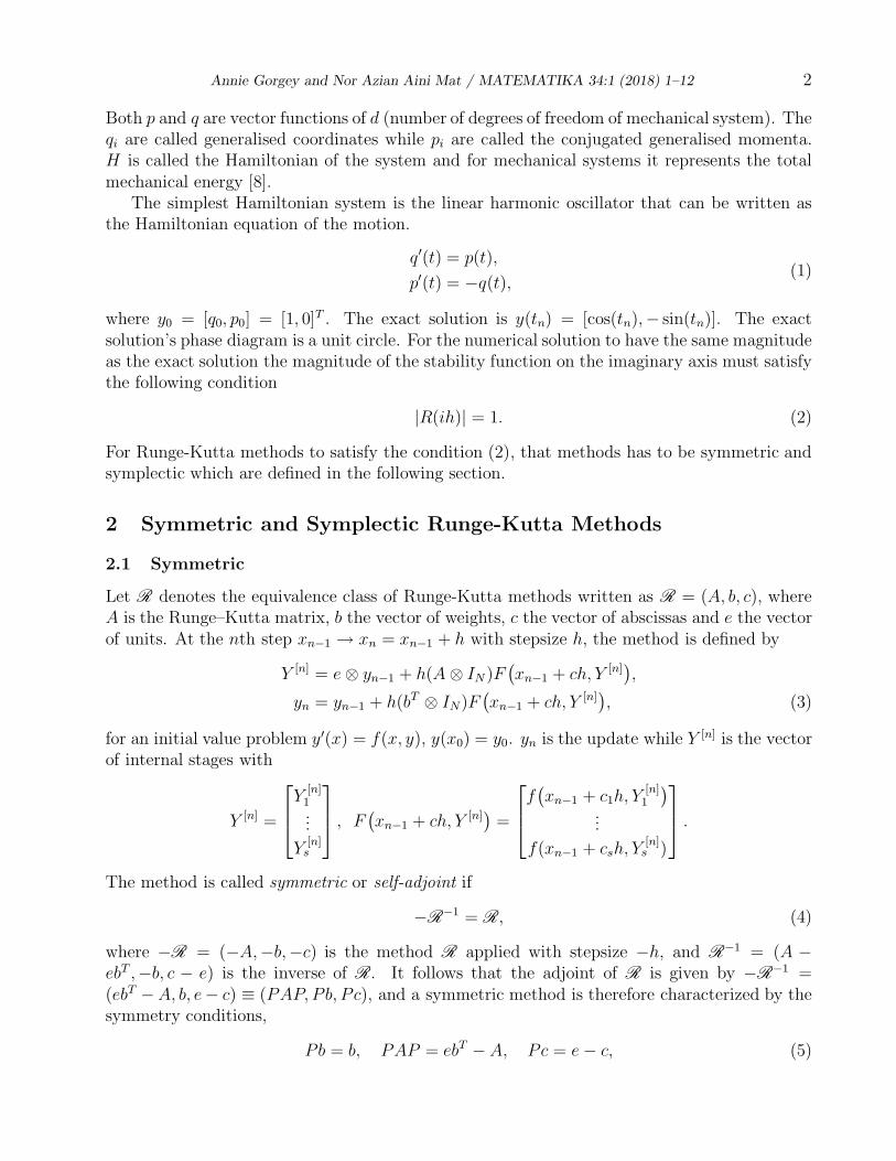
Figure 1-3 give the numerical results of IMR, ITR and 2-stage Gauss methods with passiveand active extrapolation applied to simple harmonic oscillator at different time. At tn = 10,it is shown that all these methods exhibits linear error growth as shown theoretically. Thenumerical results were also given for passive and active extrapolation. The theoretical resultsfor symmetric or symplectic methods when applied with passive and active extrapolation isgiven in another paper by the author [6]. The numerical results for active extrapolation isobserved to give the lowest error if compared with passive extrapolation. As the time increases(tn = 1000), it is shown in Figure 2 that passive extrapolation gives quadratic error growth.However, active extrapolation still gives the lowest error even with linear error growth. Figure 3shows the numerical results at tn = 1000000. All the base methods with passive extrapolationgive periodic behaviour except for active extrapolation for IMR and ITR.


−1.5 −1 −0.5 0 0.5 1−10

−9

−8

−7

−6

−5

−4

−3

−2

−1

Log10(Time)

|Log

10(E

rror)

|

IMR with passive and active extrapolation

IMR

Active IMR

Passive IMR

−1.5 −1 −0.5 0 0.5 1−10

−9

−8

−7

−6

−5

−4

−3

−2

−1

Log10(Time)

|Log

10(E

rror)

|

ITR with passive and active extrapolation

ITR

Active ITR

Passive ITR

−1.5 −1 −0.5 0 0.5 1−15

−14

−13

−12

−11

−10

−9

−8

−7

−6

−5

Log10(Time)

|Log

10(E

rror)

|

Gauss 2−stage with passive and active extrapolation

G2

Active G2

Passive G2

Figure 1: The Linear Error Growth of IMR, ITR and 2-stage Gauss Methods with Passive andActive Extrapolation in Solving Simple Harmonic Oscillator for h = 0.1 at tn = 10.


−2 −1 0 1 2 3−10

−9

−8

−7

−6

−5

−4

−3

−2

−1

0

Log10(Time)

|Log

10(E

rror)

|


IMR

Active IMR

Passive IMR

−2 −1 0 1 2 3−10

−9

−8

−7

−6

−5

−4

−3

−2

−1

0

Log10(Time)

|Log

10(E

rror)

|


ITR

Active ITR

Passive ITR

−2 −1 0 1 2 3

−14

−12

−10

−8

−6

−4

−2

Log10(Time)

|Log

10(E

rror)

|


G2

Active G2

Passive G2

Figure 2: The linear error growth of IMR, ITR and 2-stage Gauss methods with passive andactive extrapolation in solving Simple Harmonic Oscillator for h = 0.1 at tn = 1000.


−2 −1 0 1 2 3 4 5 6−10

−8

−6

−4

−2

0

2

Log10(Time)

|Log

10(E

rror)

|


IMR

Active IMR

Passive IMR

−2 −1 0 1 2 3 4 5 6−10

−8

−6

−4

−2

0

2

Log10(Time)

|Log

10(E

rror)

|


ITR

Active ITR

Passive ITR

−2 −1 0 1 2 3 4 5 6−15

−10

−5

0

Log10(Time)

|Log

10(E

rror)

|


G2

Active G2

Passive G2

Figure 3: The linear error growth of IMR, ITR and 2-stage Gauss methods with passive andactive extrapolation in solving Simple Harmonic Oscillator for h = 0.1 at tn = 1000000.


6 Conclusions

Symmetric methods such as the IMR, ITR and 2-stage Gauss are beneficial in solving Hamil-tonian problems since they are also symplectic. Symplectic methods have advantages overnon-symplectic methods in the long term integration of Hamiltonian problems. For instant, inthe simple harmonic oscillator problem, symplectic methods such as the IMR, ITR and 2-stageGauss show linear error growth. Passive and active extrapolations have been implemented toimprove the accuracy of the numerical solutions. Passive extrapolation is observed to showquadratic error growth after a very short period of time. On the other hand, active extrapola-tion is observed to show linear error growth for a much longer period of time. In addition tothat, active extrapolation is also give stable results for a longer period of time and therefore ismore advantageous on solving simple harmonic oscillator especially for IMR and ITR. However,for 2-stage Gauss method it is observed that active extrapolation gives oscillatory behaviourover long time interval. We wish to extend this study with symmetrized methods [5] and hopesymmetrization of active and passive extrapolation gives satisfying results.

Acknowledgments

The authors would like to thank the Universiti Pendidikan Sultan Idris for providing the researchgrant GPU, Vote No: 2016-0186-102-01.

References

[1] Abia, L. and Sanz-Serna, J. M. Partitioned Runge-Kutta methods for separable Hamilto-nian problems. Mathematics Computations. 1993. 60: 617–634.

[2] Burrage, K. and Butcher, J. C. Stability criteria for implicit Runge-Kutta methods. SIAMJournal of Numerical Analysis. 1979. 16: 46–57.

[3] Chan, R. P. K. and Murua, A. Extrapolation of symplectic methods for Hamiltonianproblems. Applied Numerical Mathematics. 2000. 34: 189–205.

[4] Chan, R. P. K. and Gorgey, A. Active and passive symmetrization of Runge-Kutta Gaussmethods. Applied Numerical Mathematics. 2013. 67: 64–77.

[5] Gorgey, A. and Chan, R. P. K. Choice of strategies for extrapolation with symmetrizationin the constant stepsize setting. Applied Numerical Mathematics. 2015. 87: 31–37.

[6] Gorgey, A. Extrapolation of Runge-Kutta methods in solving simple harmonic oscillatorsand simple pendulum problems. International Journal of Mathematics and Computation.2018. 29(2).

[7] Gorgey, A. Extrapolation of symmetrized Runge-Kutta methods in the variable stepsizesetting, International Journal of Applied Mathematics and Statistics, 2016. 55(2): 1–9.

[8] Hairer, E., Wanner, G. and Lubich, C. Geometric Numerical Integration: Structure-Preserving Algorithms for Ordinary Differential Equations, Springer Series in Compu-tational Mathematics. Second Edition. 4. Berlin Heidelberg: Springer-Verlag. 2006.


[9] Iserles, A. A First Course in the Numerical Analysis of Differential Equations. Second Ed.,Cambridge Text in Applied Mathematics. Cambridge University Press. 2008.

[10] Monovasilis, T., Kalogiratou, Z. and Simos, T. E. Construction of exponentially fitted sym-plectic Runge-Kutta Nystrm methods from partitioned Runge-Kutta Methods. Mediter-ranean Journal of Mathematics. 2016. 13(4): 2271–2285.

[11] Sanz-Serna, J. M. Symplectic Runge-Kutta schemes for adjoint equations, automatic dif-ferentiation, optimal control, and more. SIAM Review, 2016. 58(1): 3–33.

[12] Sanz-Serna, J. M. Runge-Kutta Schemes for Hamiltonian systems. BIT. 1988. 28: 877–883.

[13] Sanz-Serna, J. M. and Calvo, M. P. Numerical Hamiltonian problems. Applied MathematicsChapman and Mathematical Computational. 1994. 7: 500–510.

[14] Sun, G. A . Simple way constructing symplectic Runge-Kutta methods. Journal of Com-putational Mathematics. 2000. 18(1): 61–68.

[15] Tang, W., Lang, G. and Luo, X. Construction of symplectic (partitioned) Runge-Kuttamethods with continuous stage. Applied Mathematics and Computations. 2016. 286: 279–287.

[16] Zhou, W., Zhang, J., Hong, J., and Song, S. Stochastic symplectic Runge-Kutta meth-ods for the strong approximation of Hamiltonian systems with additive noise. NumericalAnalysis. 2016.1: 1–24.

eﬃciency of runge-kutta methods in solving simple harmonic

Documents