ece analog-communications
TRANSCRIPT

Analog Communication 10EC53
SJBIT/Dept of ECE Page 1
SYLLABUS ANALOG COMMUNICATION
Subject Code: 10EC53 IA Marks: 25 No. of Lecture Hrs/Week: 04
Exam Hours: 03 Total no. of Lecture Hrs: 52 Exam Marks: 100
PART – A
UNIT - 1
RANDOM PROCESS: Random variables: Several random variables. Statistical
averages: Function of Random variables, moments, Mean, Correlation and Covariance
function: Principles of autocorrelation function, cross – correlation functions. Central
limit theorem, Properties of Gaussian process. 7 Hours
UNIT - 2
AMPLITUDE MODULATION: Introduction, AM: Time-Domain description,
Frequency – Domain description. Generation of AM wave: square law modulator,
switching modulator. Detection of AM waves: square law detector, envelop detector.
Double side band suppressed carrier modulation (DSBSC): Time-Domain description,
Frequency-Domain representation, Generation of DSBSC waves: balanced modulator,
ring modulator. Coherent detection of DSBSC modulated waves. Costas loop. 7 Hours
UNIT - 3
SINGLE SIDE-BAND MODULATION (SSB): Quadrature carrier multiplexing,
Hilbert transform, properties of Hilbert transform, Pre envelope, Canonical representation
of band pass signals, Single side-band modulation, Frequency-Domain description of
SSB wave, Time-Domain description. Phase discrimination method for generating an
SSB modulated wave, Time-Domain description. Phase discrimination method for
generating an SSB modulated wave. Demodulation of SSB waves. 6 Hours
UNIT - 4
VESTIGIAL SIDE-BAND MODULATION (VSB): Frequency – Domain description,
Generation of VSB modulated wave, Time - Domain description, Envelop detection of
VSB wave plus carrier, Comparison of amplitude modulation techniques, Frequency
translation, Frequency division multiplexing, Application: Radio broadcasting, AM radio.
6 Hours
PART – B
UNIT - 5
ANGLE MODULATION (FM)-I: Basic definitions, FM, narrow band FM,wide band
FM, transmission bandwidth of FM waves, generation of FM waves: indirect FM and
direct FM. 6 Hours
UNIT - 6
ANGLE MODULATION (FM)-II: Demodulation of FM waves, FM stereo
multiplexing, Phase-locked loop, Nonlinear model of the phase – locked loop, Linear

Analog Communication 10EC53
SJBIT/Dept of ECE Page 2
model of the phase – locked loop, Nonlinear effects in FM systems.
7 Hours
UNIT - 7
NOISE: Introduction, shot noise, thermal noise, white noise, Noise equivalent
bandwidth, Narrow bandwidth, Noise Figure, Equivalent noise temperature, cascade
connection of two-port networks. 6 Hours
UNIT - 8
NOISE IN CONTINUOUS WAVE MODULATION SYSTEMS:
Introduction, Receiver model, Noise in DSB-SC receivers, Noise in SSB receivers,
Noise in AM receivers, Threshold effect, Noise in FM receivers, FM threshold effect,
Pre-emphasis and De-emphasis in FM. 7 Hours
TEXT BOOKS:
1. Communication Systems, Simon Haykins, 5th Edition, John Willey, India Pvt. Ltd,
2009.
2. An Introduction to Analog and Digital Communication, Simon Haykins, John Wiley
India Pvt. Ltd., 2008
REFERENCE BOOKS:
1. Modern digital and analog Communication systems B. P. Lathi, Oxford University
Press., 4th ed, 2010,
2. Communication Systems, Harold P.E, Stern Samy and A Mahmond, Pearson Edn,
2004.
3. Communication Systems: Singh and Sapre: Analog and digital TMH 2nd , Ed 2007.

Analog Communication 10EC53
SJBIT/Dept of ECE Page 3
INDEX SHEET
SL.NO TOPIC PAGE NO.
I UNIT – 1 RANDOM PROCESS 4-8
II UNIT – 2 AMPLITUDE MODULATION 9-24
III UNIT – 3 SINGLE SIDE-BAND
MODULATION (SSB)
25-39
IV UNIT – 4 VESTIGIAL SIDE-BAND
MODULATION
40-46
V UNIT – 5 ANGLE MODULATION (FM)-I 47-56
VI UNIT – 6 ANGLE MODULATION (FM)-II 57-62
VII UNIT – 7 NOISE: 63-67
VIII
UNIT – 8 NOISE IN CONTINUOUS
WAVE MODULATION SYSTEMS:
68-73

Analog Communication 10EC53
SJBIT/Dept of ECE Page 4
UNIT – 1
RANDOM PROCESS: Random variables: Several random variables. Statistical
averages: Function of Random variables, moments, Mean, Correlation and Covariance
function: Principles of autocorrelation function, cross – correlation functions. Central
limit theorem, Properties of Gaussian
process. 7 Hrs
TEXT BOOKS:
1. Communication Systems, Simon Haykins, 5th Edition, John Willey, India Pvt. Ltd,
2009.
2. An Introduction to Analog and Digital Communication, Simon Haykins, John
Wiley India Pvt. Ltd., 2008
REFERENCE BOOKS:
1. Modern digital and analog Communication systems B. P. Lathi, Oxford University
Press., 4th ed, 2010
2. Communication Systems, Harold P.E, Stern Samy and A Mahmond, Pearson Edn,
2004.
3. Communication Systems: Singh and Sapre: Analog and digital TMH 2nd , Ed 2007.

Analog Communication 10EC53
SJBIT/Dept of ECE Page 5
1.1. Random Process
A random process is a signal that takes on values, which are determined (at least in part)
by chance. A sinusoid with amplitude that is given by a random variable is an example of
a random process. A random process cannot be predicted precisely. However, a
deterministic signal is completely predictable.
An ergodic process is one in which time averages may be used to replace ensemble
averages. As signals are often functions of time in signal processing applications,
egodicity is a useful property. An example of an ensemble average is the mean win at the
blackjack tables across a whole casino, in one day. A similar time average could be the
mean win at a particular blackjack table over every day for a month, for example. If these
averages were approximately the same, then the process of blackjack winning would
appear to be ergodic. Ergodicity can be difficult to prove or demonstrate, hence it is often
simply assumed.
1.2. Probabilistic Description of a Random Process
Although random processes are governed by chance, more typical values and trends in
the signal value can be described. A probability density function can be used to describe
the typical intensities of the random signal (over all time). An autocorrelation function
describes how similar the signal values are expected to be at two successive time
instances. It can distinguish between „erratic‟ signals versus a „lazy random walk‟.
Probability Theory:
Statistics is branch of mathematics that deals with the collection of data. It also concerns
with what can be learned from data. Extension of statistical theory is Probability Theory.
Probability deals with the result of an experiment whose actual outcome is not known. It
also deals with averages of mass phenomenon. The experiment in which the Outcome
cannot be predicted with certainty is called Random Experiment. These experiments can
also be referred to as a probabilistic experiment in which more than one thing can
happen. Eg: Tossing of a coin, throwing of a dice.
Deterministic Model and Stochastic Model or Random Mathematical Mode can be used
to describe a physical phenomenon. In Deterministic Model there is no uncertainty about
its time dependent behavior. A sample point corresponds to the aggregate of all possible
outcomes. Sample space or ensemble composed of functions of time-Random Process or
stochastic Process.
Types of Random Variable(RV):
1. Discrete Random Variable: An RV that can take on only a finite or countably infinite
set of outcomes.
2. Continuous Random Variable: An RV that can take on any value along a continuum
(but may be reported “discretely”).Random Variables are denoted by upper case letters
(Y).Individual outcomes for RV are denoted by lower case letters (y).

Analog Communication 10EC53
SJBIT/Dept of ECE Page 6
Discrete Random Variable:
Discrete Random Variable are the ones that takes on a countable number of values this
means you can sit down and list all possible outcomes without missing any, although it
might take you an infinite amount of time.
X = values on the roll of two dice: X has to be either 2, 3, 4, …, or 12.
Y = number of accidents on the UTA campus during a week: Y has to be 0, 1, 2, 3, 4, 5,
6, 7, 8, ……………”real big number” Probability Distribution: Table, Graph, or Formula
that describes values a random variable can take on, and its corresponding probability
(discrete RV) or density (continuous RV).
1. Discrete Probability Distribution: Assigns probabilities (masses) to the individual
outcomes.
2. Continuous Probability Distribution: Assigns density at individual points, probability
of ranges can be obtained by integrating density function.
3. Discrete Probabilities denoted by: p(y) = P(Y=y)
4. Continuous Densities denoted by: f(y)
5. Cumulative Distribution Function: F(y) = P(Y<=y)
For a discrete random variable, we have a probability mass function (pmf).The pmf looks
like a bunch of spikes, and probabilities are represented by the heights of the spikes. For a
continuous random. variable, we have a probability density function (pdf). The pdf looks
like a curve, and probabilities are represented by areas under the curve.
Continuous Random Variable:
Continuous Random Variable is usually measurement data [time, weight, distance, etc]
the one that takes on an uncountable number of values this means you can never list all
possible outcomes even if you had an infinite amount of time.
X = time it takes you to drive home from class: X > 0, might be 30.1 minutes measured to
the nearest tenth but in reality the actual time is 30.10000001…………………. minutes?)
A continuous random variable has an infinite number of possible values & the probability
of any one particular value is zero.
1.3. Autocorrelation
If the autocorrelation for a process depends only on the time difference t2 – t1, then the
random process is deemed „wide sense stationary‟. For a WSS process:
For a WSS, ergodic, process autocorrelation may be evaluated via a time average
(Autocorrelation function, for continuous-time)
(Autocorrelation sequence, for discrete-time)

Analog Communication 10EC53
SJBIT/Dept of ECE Page 7
Crosscorrelation Function for a Stationary Process
1.4. Power Spectral Density
For a stationary process, the Wiener-Khinchine relation states:
Where denotes Fourier transform. can be thought of as the „expected power‟ of the
random process. This is because
Where is a truncated version of the random process. The quantity
is known as the periodogram of X(t). The PSD may be estimated computationally, by
taking the average of many examples of the power spectrum, over a relatively long
intervals of the process X(t). This reveals the expected power density at various
frequencies. (One such interval of X(t) would not typically have the power density of the
time averaged version).
Recommended questions:
1. Define mean, Auto correlation and auto co variance of a random process 2. Define power spectral density and explain its properties. 3. Explain cross correlation and Auto correlation. 4. State the properties of Gaussian process? 5. Define conditional probability, Ramdom variable amd mean? 6. Explain Joint probability of the events A & B? 7. Explain Conditional probability of the events A & B? 8. Explain the properties Gaussian process? 9. Compare auto correlation and cross correlation functions?

Analog Communication 10EC53
SJBIT/Dept of ECE Page 8
UNIT - 2
AMPLITUDE MODULATION
Introduction, AM: Time-Domain description, Frequency – Domain description.
Generation of AM wave: square law modulator, switching modulator. Detection of AM
waves: square law detector, envelop detector. Double side band suppressed carrier
modulation (DSBSC): Time-Domain description, Frequency-Domain representation,
Generation of DSBSC waves: balanced modulator, ring modulator. Coherent detection of
DSBSC modulated waves. Costas loop. 7 Hrs
TEXT BOOKS:
1. Communication Systems, Simon Haykins, 5th Edition, John Willey, India Pvt. Ltd,
2009.
2. An Introduction to Analog and Digital Communication, Simon Haykins, John
Wiley India Pvt. Ltd., 2008
REFERENCE BOOKS:
1. Modern digital and analog Communication systems B. P. Lathi, Oxford University
Press., 4th ed, 2010
2. Communication Systems, Harold P.E, Stern Samy and A Mahmond, Pearson Edn,
2004.
3. Communication Systems: Singh and Sapre: Analog and digital TMH 2nd , Ed 2007.

Analog Communication 10EC53
SJBIT/Dept of ECE Page 9
2.1. Introduction Modulation is a process of varying one of the characteristics of high frequency sinusoidal
(the carrier) in accordance with the instantaneous values of the modulating (the
information) signal. The high frequency carrier signal is mathematically represented by
the equation 2.1.
Where c(t )--instantaneous values of the cosine wave
Ac --its maximum value
fc --carrier frequency
--phase relation with respect to the reference
Any of the last three characteristics or parameters of the carrier can be varied by the
modulating (message) signal, giving rise to amplitude, frequency or phase modulation
respectively.
Need for modulation: 1. Practicability of antenna
In the audio frequency range, for efficient radiation and reception, the transmitting and
receiving antennas must have sizes comparable to the wavelength of the frequency of the
signal used. It is calculated using the relation f = c . The wavelength is 75 meters at
1MHz in the broadcast band, but at 1 KHz, the wavelength turns out to be 300
Kilometers. A practical antenna for this value of wavelength is unimaginable and
impossible.
2. Modulation for ease of radiation
For efficient radiation of electromagnetic waves, the antenna dimension required is of
the order of /4 to l/2. It is possible to construct practical antennas only by
increasing the frequency of the base band signal.
3. Modulation for multiplexing
The process of combining several signals for simultaneous transmission on a single
channel is called multiplexing. In order to use a channel to transmit the different base
band signals (information) at the same time, it becomes necessary to translate different
signals so as to make them occupy different frequency slots or bands so that they do not
interfere. This is a accomplished by using carrier of different frequencies.
4. Narrow banding
Suppose that we want to transmit audio signal ranging from 50 - 104 Hz using suitable
antenna. The ratio of highest to lowest frequency is 200. Therefore an antenna suitable
for use at one end of the frequency range would be entirely too short or too long for the
other end. Suppose that the audio spectrum is translated so that it occupies the range from
50+106 to 10
4+10
6 Hz. Then the ratio of highest to lowest frequency becomes 1.01. Thus
the process of frequency translation is useful to change wideband signals to narrow band
signals.
At lower frequencies, the effects of flicker noise and burst noise are severe.

Analog Communication 10EC53
SJBIT/Dept of ECE Page 10
2.2 Amplitude modulation
In amplitude modulation, the amplitude of the carrier signal is varied by the
modulating/message/information/base-band signal, in accordance with the instantaneous
values of the message signal. That is amplitude of the carrier is made proportional to the
instantaneous values (amplitude) of the modulating signal. If m(t) is the information
signal and c(t) = Ac cos ( 2πfct + ) is the carrier, the amplitude of the carrier signal is
varied proportional to the m(t ) .
The peak amplitude of carrier after modulation at any instant is given by [ Ac+ m(t .
The carrier signal after modulation or the modulated signal is represented by the equation
2.2.
Where
is called amplitude sensitivity of the modulator.
The equation (2.3) is the standard expression for Amplitude Modulated signal.
Let m(t )= Am cos ( 2πfmt) be the message signal of frequency fm and peak amplitude Am.
Then single-tone modulated signal is given by the equation 2.4.
The modulation index m of AM system is defined as the ratio of peak amplitude of
message signal to peak amplitude of carrier signal.
The following figure 2.1 shows the message, carrier and amplitude modulated
waveforms.
Carrier wave

Analog Communication 10EC53
SJBIT/Dept of ECE Page 11
Modulating wave
AM wave
Figure 2.1: message, carrier and amplitude modulated signal
Note:
(1) m is also called depth of modulation.
(2) m specifies the system clarity. As m increases, the system clarity also increases.
Consider the Amplitude Modulated waveform shown in figure 2.2.
Figure 2.2: Message and amplitude modulated signal
We have the modulation index given by
From the figure 2.2, we get

Analog Communication 10EC53
SJBIT/Dept of ECE Page 12
Dividing the equation (2.7) by (2.9), we get
Here Amax is the maximum amplitude and Amin is minimum amplitude of the modulated
signal.
Modulation index m has to be governed such that it is always less than unity; otherwise it
results in a situation known as „over-modulation‟ (m>1). The over modulation occurs,
whenever the magnitude of the peak amplitude of the modulating signal exceeds the
magnitude of the peak amplitude of the carrier signal. The signal gets distorted due to
over modulation. Because of this limitation on „m ‟, the system clarity is also limited. The
AM waveforms for different values of modulation index m are as shown in figure 2.3.
Figure 2.3: AM waveforms for different values of m
Note: If the modulation index exceeds unity the negative peak of the modulating
waveform is clipped and [Ac+ m(t )] goes negative, which mathematically appears as a
phase reversal rather than a clamped level.
2.3 Single tone Amplitude Modulation/ Sinusoidal AM
Consider a modulating wave m(t) that consists of a single tone or single frequency
component given by
where Am is peak amplitude of the sinusoidal modulating wave. fm is the frequency of
the sinusoidal modulating wave
Let Ac be the peak amplitude and fc be the frequency of the high frequency carrier
signal. Then the corresponding single-tone AM wave is given by
Let Amax and Amin denote the maximum and minimum values of the envelope of
the modulated wave. Then from the above equation (2.12), we get
Analog Communication 10EC53
SJBIT/Dept of ECE Page 13
Expanding the equation (2.12), we get
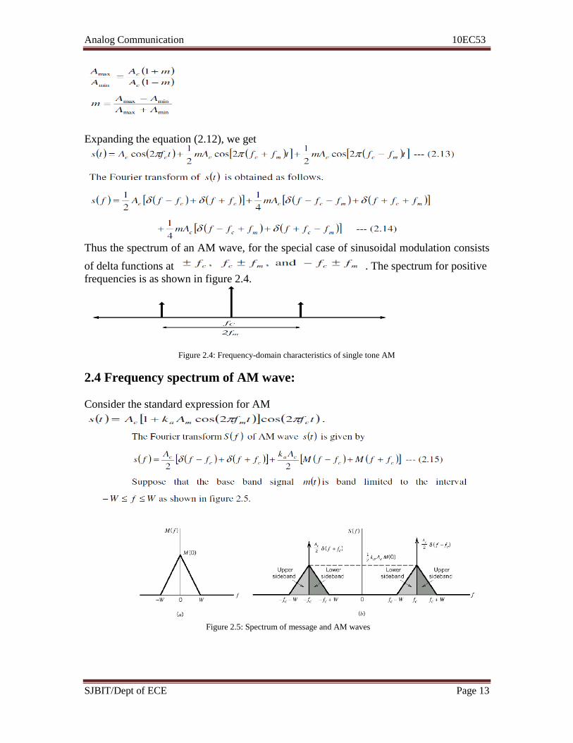
Thus the spectrum of an AM wave, for the special case of sinusoidal modulation consists
of delta functions at . The spectrum for positive
frequencies is as shown in figure 2.4.
Figure 2.4: Frequency-domain characteristics of single tone AM
2.4 Frequency spectrum of AM wave:
Consider the standard expression for AM
Figure 2.5: Spectrum of message and AM waves

Analog Communication 10EC53
SJBIT/Dept of ECE Page 14
2.5 Average power for sinusoidal AM (Power relations in AM)
Consider the expression for single tone/sinusoidal AM wave
This expression contains three components. They are carrier component, upper side band
and lower side band. Therefore Average power of the AM wave is sum of these three
components.
Therefore the total power in the amplitude modulated wave is given by
The ratio is called the efficiency of AM system and it takes maximum value of 33% at
m=1.
2.6 Effective voltage and current for sinusoidal AM
In AM systems, the modulated and unmodulated currents are necessary to calculate the
modulation index from them.
The effective or rms value of voltage Et of the modulated wave is defined by the equation

Analog Communication 10EC53
SJBIT/Dept of ECE Page 15
Similarly the effective or root mean square voltage Ec of carrier component is defined by
Where It is the rms current of modulated wave and Ic is the rms current of unmodulated
carrier.
Note: The maximum power in the AM wave is Pt = 1.5Pc, when m=1. This is important,
because it is the maximum power that relevant amplifiers must be capable of handling
without distortion.
2.7 Non sinusoidal Modulation
When a sinusoidal carrier signal is modulated by a non-sinusoidal modulating signal, the
process is called Non-sinusoidal modulation. Consider a high frequency sinusoidal signal
and the non-sinusoidal message signal m(t) as shown in figure 2.6. The non-sinusoidal
modulating signal has a line spectrum that is many frequency components of different
amplitudes.
Figure 2.6: Non-sinusoidal message signal and spectrum
The expression for the non-sinusoidal AM is given by
Amplitude Modulators
Two basic amplitude modulation principles are discussed. They are square law
modulation and switching modulation.

Analog Communication 10EC53
SJBIT/Dept of ECE Page 16
Square law modulator
When the output of a device is not directly proportional to input throughout the operation,
the device is said to be non-linear. The Input-Output relation of a non-linear device can
be expressed as
When the in put is very small, the higher power terms can be neglected. Hence the output
is approximately given by
When the output is considered up to square of the input, the device is called a square law
device and the square law modulator is as shown in the figure 2.7.
Figure 2.7: Square law modulator
Consider a non linear device to which a carrier c(t)= Ac cos(2π f ct) and an information
signal m(t) are fed simultaneously as shown in figure 2.7. The total input to the device at
any instant is
Therefore the square law device output 0 V consists of the dc component at f = 0.
The information signal ranging from 0 to W Hz and its second harmonics. Signal at fc and

Analog Communication 10EC53
SJBIT/Dept of ECE Page 17
Frequency band centered at c f with a deviation of +-W , Hz.
The required AM signal with a carrier frequency fc can be separated using a band pass
filter at the out put of the square law device. The filter should have a lower cutoff
frequency ranging between 2W and (fc -W) and upper cut-off frequency between (fc +W)
and 2 fc
Therefore the filter output is
Switching modulator
Consider a semiconductor diode used as an ideal switch to which the carrier signal c(t)=
Ac cos(2π f ct) and information signal m(t) are applied simultaneously as shown figure
2.8.
Figure 2.8: Switching modulator
The total input for the diode at any instant is given by
When the peak amplitude of c(t) is maintained more than that of information signal, the
operation is assumed to be dependent on only c(t) irrespective of m(t). When c(t) is
positive, v2=v1since the diode is forward biased. Similarly, when c(t) is negative, v2=0
since diode is reverse biased. Based upon above operation, switching response of the
diode is periodic rectangular wave with an amplitude unity and is given by

Analog Communication 10EC53
SJBIT/Dept of ECE Page 18
The diode output v2 consists of a dc component at f =0.
Information signal ranging from 0 to w Hz and infinite number of frequency bands
centered at f, 2fc, 3fc, 4fc, ---------
The required AM signal centered at fc can be separated using band pass filter. The lower
cutoff-frequency for the band pass filter should be between w and fc-w and the upper cut-
off frequency between fc+w and 2fc. The filter output is given by the equation
The output AM signal is free from distortions and attenuations only when fc-w>w or
fc>2w.
Demodulation of AM: - Demodulation is the process of recovering the information signal (base band) from the
incoming modulated signal at the receiver. There are two methods.

Analog Communication 10EC53
SJBIT/Dept of ECE Page 19
Square law demodulator
Consider a non-linear device to which the AM signal s(t) is applied. When the level of
s(t) is very small, output can be considered upto square of the input.
Figure 2.9: Demodulation of AM using square law device
The device output consists of a dc component at f =0, information signal ranging from 0-
W Hz and its second harmonics and frequency bands centered at fc and 2fc. The required
information can be separated using low pass filter with cut off frequency ranging between
W and fc-w.
The filter output is given by
DC component + message signal + second harmonic

Analog Communication 10EC53
SJBIT/Dept of ECE Page 20
The dc component (first term) can be eliminated using a coupling capacitor or a
transformer. The effect of second harmonics of information signal can be reduced by
maintaining its level very low. When m(t) is very low, the filter output is given by
When the information level is very low, the noise effect increases at the receiver, hence
the system clarity is very low using square law demodulator.
Envelop detector
It is a simple and highly effective system. This method is used in most of the commercial
AM radio receivers. An envelope detector is as shown below.
Figure 2.10: Envelope detector
During the positive half cycles of the input signals, the diode D is forward biased and the
capacitor C charges up rapidly to the peak of the input signal. When the input signal falls
below this value, the diode becomes reverse biased and the capacitor C discharges
through the load resistor RL.
The discharge process continues until the next positive half cycle. When the input signal
becomes greater than the voltage across the capacitor, the diode conducts again and the
process is repeated.
The charge time constant (rf+Rs)C must be short compared with the carrier period, the
capacitor charges rapidly and there by follows the applied voltage up to the positive peak
when the diode is conducting.
That is the charging time constant shall satisfy the condition,
On the other hand, the discharging time-constant RLC must be long enough to ensure that
the capacitor discharges slowly through the load resistor RL between the positive peaks
of the carrier wave, but not so long that the capacitor voltage will not discharge at the
maximum rate of change of the modulating wave.
That is the discharge time constant shall satisfy the condition,
where „W‟ is band width of the message signal.
The result is that the capacitor voltage or detector output is nearly the same as the
envelope of AM wave.

Analog Communication 10EC53
SJBIT/Dept of ECE Page 21
Advantages of AM: Generation and demodulation of AM wave are easy. AM systems are
cost effective and easy to build.
Disadvantages: AM contains unwanted carrier component, hence it requires more
transmission power. The transmission bandwidth is equal to twice the message
bandwidth.
To overcome these limitations, the conventional AM system is modified at the cost of
increased system complexity. Three types of modified AM systems are
1. DSBSC (Double Side Band Suppressed Carrier) modulation
2. SSBSC (Single Side Band Suppressed Carrier) modulation
3. VSB (Vestigial Side Band) modulation
In DSBC modulation, the modulated wave consists of only the upper and lower side
bands. Transmitted power is saved through the suppression of the carrier wave, but
the channel bandwidth requirement is the same as before.
The SSBSC modulated wave consists of only the upper side band or lower side band.
SSBSC is suited for transmission of voice signals. It is an optimum form of modulation in
that it requires the minimum transmission power and minimum channel band width.
Disadvantage is increased cost and complexity.
In VSB, one side band is completely passed and just a trace or vestige of the other side
band is retained. The required channel bandwidth is therefore in excess of the message
bandwidth by an amount equal to the width of the vestigial side band. This method is
suitable for the transmission of wide band signals.
Double Side Band Suppressed Carrier Modulation
DSBSC modulators make use of the multiplying action in which the modulating signal
multiplies the carrier wave. In this system, the carrier component is eliminated and both
upper and lower side bands are transmitted. As the carrier component is suppressed, the
power required for transmission is less than that of AM.
If m(t) is the message signal and c(t)= Ac cos(2π f ct) is the carrier signal, then DSBSC
modulated wave s(t) is given by
Consequently, the modulated signal s(t) under goes a phase reversal , whenever the
message signal m(t) crosses zero as shown below.

Analog Communication 10EC53
SJBIT/Dept of ECE Page 22
Figure2.11: Carrier, message and DSBSC wave forms
The envelope of a DSBSC modulated signal is therefore different from the message
signal and the Fourier transform of s(t) is given by
For the case when base band signal m(t) is limited to the interval –W<f<W as shown in
figure below, we find that the spectrum S(f) of the DSBSC wave s(t) is as illustrated
below. Except for a change in scaling factor, the modulation process simply translates the
spectrum of the base band signal by fc. The transmission bandwidth required by DSBSC
modulation is the same as that for AM.
Figure2.12: Message and the corresponding DSBSC spectrum
Ring modulator
Ring modulator is the most widely used product modulator for generating DSBSC wave
and is shown below.

Analog Communication 10EC53
SJBIT/Dept of ECE Page 23
Figure 2.13: Ring modulator
The four diodes form a ring in which they all point in the same direction. The diodes are
controlled by square wave carrier c(t) of frequency fc, which is applied longitudinally by
means of two center-tapped transformers. Assuming the diodes are ideal, when the carrier
is positive, the outer diodes D1 and D2 are forward biased where as the inner diodes D3
and D4 are reverse biased, so that the modulator multiplies the base band signal m(t) by
c(t). When the carrier is negative, the diodes D1 and D2 are reverse biased and D3 and
D4 are forward, and the modulator multiplies the base band signal –m(t) by c(t). Thus the
ring modulator in its ideal form is a product modulator for square wave carrier and the
base band signal m(t). The square wave carrier can be expanded using Fourier series as
Therefore the ring modulator out put is given by
From the above equation it is clear that output from the modulator consists entirely of
modulation products. If the message signal m(t) is band limited to the frequency band
–w< f<w, the output spectrum consists of side bands centered at fc.
Balance modulator (Product modulator)
A balanced modulator consists of two standard amplitude modulators arranged in a
balanced configuration so as to suppress the carrier wave as shown in the following block
diagram. It is assumed that the AM modulators are identical, except for the sign reversal
of the modulating wave applied to the input of one of them. Thus, the output of the two
modulators may be expressed as,
Figure 2.14: Balanced modulator

Analog Communication 10EC53
SJBIT/Dept of ECE Page 24
Subtracting s2(t) from s1(t),
Hence, except for the scaling factor 2ka, the balanced modulator output is equal to the
product of the modulating wave and the carrier.
Demodulation of DSBSC modulated wave by Coherent detection
The message signal m(t) can be uniquely recovered from a DSBSC wave s(t) by first
multiplying s(t) with a locally generated sinusoidal wave and then low pass filtering the
product as shown.
Figure 2.15: Coherent detector
It is assumed that the local oscillator signal is exactly coherent or synchronized, in both
frequency and phase, with the carrier wave c(t) used in the product modulator to generate
s(t). This method of demodulation is known as coherent detection or synchronous
detection.
Let Ac1 cos ( 2πfct + ) be the local oscillator signal, and s(t) = Ac cos ( 2πfct) m(t) be the
DSBSC wave. Then the product modulator output v(t) is given by
The first term in the above expression represents a DSBSC modulated signal with a
carrier frequency 2fc, and the second term represents the scaled version of message
signal. Assuming that the message signal is band limited to the interval −<w <f<w, the
spectrum of v(t) is plotted as shown below.

Analog Communication 10EC53
SJBIT/Dept of ECE Page 25
Figure2.16: Spectrum of output of the product modulator
From the spectrum, it is clear that the unwanted component (first term in the expression)
can be removed by the low-pass filter, provided that the cut-off frequency of the filter is
greater than W but less than 2fc-W. The filter output is given by
The demodulated signal vo(t) is therefore proportional to m(t) when the phase error is
constant.
Single tone DSBSC modulation
Consider a sinusoidal modulating signal m(t)=Am cos ( 2πfmt) of single frequency and the
carrier signal c(t)=Ac cos ( 2πfct).
The corresponding DSBSC modulated wave is given by
Thus the spectrum of the DSBSC modulated wave, for the case of sinusoidal modulating
wave, consists of delta functions located at .
Assuming perfect synchronism between the local oscillator and carrier wave in a coherent
detector, the product modulator output contains the high frequency components and
scaled version of original information signal. The Low Pass Filter is used to separate the
desired message signal.
Costas Receiver (Costas loop) Costas receiver is a synchronous receiver system, suitable for demodulating DSBSC
waves. It consists of two coherent detectors supplied with the same input signal, that is
the incoming DSBSC wave but with individual local oscillator signals that are in phase
quadrature with respect to each other as shown below.
Figure 2.17 : Costas receiver

Analog Communication 10EC53
SJBIT/Dept of ECE Page 26
The frequency of the local oscillator is adjusted to be the same as the carrier frequency fc.
The detector in the upper path is referred to as the in-phase coherent detector or Ichannel,
and that in the lower path is referred to as the quadrature-phase coherent detector or Q-
channel. These two detector are coupled together to form a negative feed back system
designed in such a way as to maintain the local oscillator synchronous with the carrier
wave. Suppose the local oscillator signal is of the same phase as the carrier wave
c(t)=Accos ( 2πfct) used to generate the incoming DSBSC wave. Then we find that the I-
channel output contains the desired demodulated signal m(t), where as the Qchannel
output is zero due to quadrature null effect of the Q-channel. Suppose that the local
oscillator phase drifts from its proper value by a small angle radiations. The Ichannel
output will remain essentially unchanged, but there will be some signal appearing at the
Q-channel output, which is proportional to sin( )= for small . This Q-channel output
will have same polarity as the I-channel output for one direction of local oscillator phase
drift and opposite polarity for the opposite direction of local oscillator phase drift. Thus
by combining the I-channel and Q-channel outputs in a phase discriminator (which
consists of a multiplier followed by a LPF), a dc control signal is obtained that
automatically corrects for the local phase errors in the voltage-controlled oscillator.
Recommended questions:
1. Explain the need for Modulation?
2. Explain the generation of AM wave using switching modulator with equations,
waveforms and spectrum before and after filtering process?
3. Explain the time domain & frequency domain representation of AM wave?
4. Show that square law device can be used to detect AM wave?
5. Explain the generation of DSB-SC using Balanced modulator?
6. What is Quadrature null effect? How it can be eliminate?
7. Explain the generation of DSB-SC using Ring modulator?
8. With a neat diagram explain quadrature carrier multiplexing?
9. Define Demodulation?
10. Explain single tone AM with necessary waveforms?
Analog Communication 10EC53
SJBIT/Dept of ECE Page 27
UNIT – 3
SINGLE SIDE-BAND MODULATION (SSB)
Quadrature carrier multiplexing, Hilbert transform, properties of Hilbert transform,
preenvelope, Canonical representation of band pass signals, Single side-band modulation,
Frequency-Domain description of SSB wave, Time-Domain description. Phase
discrimination method for generating an SSB modulated wave, Time-Domain
description. Phase discrimination method for generating an SSB modulated wave.
Demodulation of SSB waves. 6 Hrs
TEXT BOOKS:
1. Communication Systems, Simon Haykins, 5th Edition, John Willey, India Pvt. Ltd,
2009.
2. An Introduction to Analog and Digital Communication, Simon Haykins, John
Wiley India Pvt. Ltd., 2008
REFERENCE BOOKS:
1. Modern digital and analog Communication systems B. P. Lathi, Oxford University
Press., 4th ed, 2010
2. Communication Systems, Harold P.E, Stern Samy and A Mahmond, Pearson Edn,
2004.
3. Communication Systems: Singh and Sapre: Analog and digital TMH 2nd , Ed 2007.

Analog Communication 10EC53
SJBIT/Dept of ECE Page 28
3.1 Quadrature Carrier Multiplexing
A Quadrature Carrier Multiplexing (QCM) or Quadrature Amplitude Modulation (QAM)
method enables two DSBSC modulated waves, resulting from two different message
signals to occupy the same transmission band width and two message signals can be
separated at the receiver. The transmitter and receiver for QCM are as shown in figure
3.1.
Figure 3.1 QCM transmitter and receiver
The transmitter involves the use of two separate product modulators that are supplied
with two carrier waves of the same frequency but differing in phase by -90o. The
multiplexed signal s(t) consists of the sum of the two product modulator outputs given by
the equation 3.1.
where m1(t) and m2(t) are two different message signals applied to the product
modulators. Thus, the multiplexed signal s(t) occupies a transmission band width of 2W,
centered at the carrier frequency fc where W is the band width of message signal m1(t) or
m2(t), whichever is larger.
At the receiver, the multiplexed signal s(t) is applied simultaneously to two separate
coherent detectors that are supplied with two local carriers of the same frequency but
differing in phase by -90o. The output of the top detector is and that of the
bottom detector .
For the QCM system to operate satisfactorily, it is important to maintain correct phase
and frequency relationships between the local oscillators used in the transmitter and
receiver parts of the system.
3.2 Hilbert transform
The Fourier transform is useful for evaluating the frequency content of an energy signal,
or in a limiting case that of a power signal. It provides mathematical basis for analyzing
and designing the frequency selective filters for the separation of signals on the basis of
their frequency content. Another method of separating the signals is based on phase

Analog Communication 10EC53
SJBIT/Dept of ECE Page 29
selectivity, which uses phase shifts between the appropriate signals (components) to
achieve the desired separation.
In case of a sinusoidal signal, the simplest phase shift of 180o is obtained by “Ideal
transformer” (polarity reversal). When the phase angles of all the components of a given
signal are shifted by 90o, the resulting function of time is called the “Hilbert transform”
of the signal.
Consider an LTI system with transfer function defined by equation 3.2.
The device which possesses such a property is called Hilbert transformer. When ever a
signal is applied to the Hilbert transformer, the amplitudes of all frequency components
of the input signal remain unaffected. It produces a phase shift of -90o for all positive
frequencies, while a phase shift of 90o for all negative frequencies of the signal.
If x(t) is an input signal, then its Hilbert transformer is denoted by xˆ(t ) and shown in the
following diagram.

Analog Communication 10EC53
SJBIT/Dept of ECE Page 30
To find impulse response h(t) of Hilbert transformer with transfer function H(f):
Consider the relation between Signum function and the unit step function.
We have
Therefore the impulse response h(t) of an Hilbert transformer is given by the equation
3.4,
Now consider any input x(t) to the Hilbert transformer, which is an LTI system. Let the
impulse response of the Hilbert transformer is obtained by convolving the input x(t) and
impulse response h(t) of the system.

Analog Communication 10EC53
SJBIT/Dept of ECE Page 31
Applications of Hilbert transform 1. It is used to realize phase selectivity in the generation of special kind of modulation
called Single Side Band modulation.
2. It provides mathematical basis for the representation of band pass signals.
Note: Hilbert transform applies to any signal that is Fourier transformable.
3.3 Pre-envelope
Consider a real valued signal x(t). The pre-envelope x+ (t ) for positive frequencies of
the signal x(t) is defined as the complex valued function given by equation 3.8.
The pre-envelope x -(t ) for negative frequencies of the signal is given by
The spectrum of the pre-envelope x+ (t ) is nonzero only for positive frequencies as
emphasized in equation 3.9. Hence plus sign is used as a subscript. In contrast, the
spectrum of the other pre-envelope x -(t ) is nonzero only for negative frequencies. That is
Figure 3.2: Spectrum of the low pass signal x(t)

Analog Communication 10EC53
SJBIT/Dept of ECE Page 32
Figure 3.3: Spectrum of pre-envelope x (t ) +
Properties of Hilbert transform
1. “A signal x(t) and its Hilbert transform xˆ(t )have the same amplitude spectrum”. The
magnitude of –jsgn(f) is equal to 1 for all frequencies f. Therefore x(t) and xˆ(t ) have the
same amplitude spectrum.
That is Xˆ ( f ) = X ( f ) for all f.
2. “If xˆ(t ) is the Hilbert transform of x(t), then the Hilbert transform of xˆ(t ), is –x(t)”.
To obtain its Hilbert transform of x(t), x(t) is passed through a LTI system with a transfer
function equal to –jsgn(f). A double Hilbert transformation is equivalent to passing x(t)
through a cascade of two such devices. The overall transfer function of such a cascade is
equal to
The resulting output is –x(t). That is the Hilbert transform of xˆ(t ) is equal to –x(t).
Canonical representation for band pass signal
The Fourier transform of band-pass signal contains a band of frequencies of total extent
2W. The pre-envelope of a narrow band signal x(t) is given by

Analog Communication 10EC53
SJBIT/Dept of ECE Page 33
Figure 3.4 shows the amplitude spectrum of band pass signal x(t). Figure 3.5 shows
amplitude spectrum of pre envelope x+ (t ). Figure 3.6 shows amplitude spectrum of
complex envelope .
Filtering of side bands:
An intuitively satisfying method of achieving this requirement is frequency
discrimination method that involves the use of an appropriate filter following a product
modulator responsible for the generation of the DSBSC modulated signal
Consider the following circuit
m(t)cos(2
Let H(f) denote the transfer function of the filter following the product modulator. The
spectrum of the modulated signal s(t) produced by passing u(t) though filter is given by
Where M(f) is the Fourier transform of the message signal m(t). the problem we wish to
address is to determine the particular H(f) required to produce a modulated signal s(t)
with desired spectral characteristics, such that the original message signal m(t) may be
recovered from s(t) by coherent detection
The first step involves multiplying the modulated signal s(t) by a locally generated
sinusoidal wave which is synchronous with the carrier wave in both frequency and phase.
Thus we may write
Transforming this relation into frequency domain gives the Fourier transform of v(t) as
The high frequency components of v(t) represented by the second term in the equation
are removed by the low pass filter to produce an output the spectrum is given by
the remaining components
For a distortion less reproduction of the original signal m(t) at the coherent detector
output we require to be scaled version of M(f) . this means the transfer function
H(f) should satisfy the condition
Where H(fc) the value of H(f) at f = fc is a constant. When the message spectrum M(f) is
outside the frequency range –W <= f <= W we need satisfy only the above equation for
the values of f in this interval. Also to , simplify the exposition we set H(fc) = ½ . thus
require H(f) satisfies the condition
The coherent detector output is given by

Analog Communication 10EC53
SJBIT/Dept of ECE Page 34
The above equations defines the spectrum of the modulated signal s(t) is a band pass
signal we may formulate its time domain description in terms of in phase and quadrature
components using the pass band signal method s(t) may be expressed in the canonical
form
Where is the in phase component and is the quadrature component
To determine
Hence substituting , we find the Fourier transform of is given by
=
To determine the quadrature component of the modulated signal s(t),
We can recover the message signal by passing through certain filters whose transfer
function is as follows
Let m‟(t) denote output message signal
m(t)=
the in phase component is completely independent of the transfer function H(f) of the
pass band filter involved in the generation of the modulated wave
the spectral modification attributed to the transfer function H(f) is confined solely to the
quadrature component
The role of the quadrature component is merely to interfere with the in phase component
so as to reduce or eliminate power in one of the side bands of the modulated signal s(t)
depending on the application of interest.
3.4. Single-side band modulation:

Analog Communication 10EC53
SJBIT/Dept of ECE Page 35
Standard amplitude modulation and DSBSC are wasteful of bandwidth beause they both
require a transmission bandwidth equal twice the message bandwidth
Thus the channel needs to provide only the same bandwidth as the message signal. When
only one side band is transmitted the modulation is reffered to as single side band
modulation.
3.4.1. Frequency domain description:
Precise frequency domain description of a single side band modulation wave depends on
which side band is transmitted.
Consider a messge signal M(f) limited to the band . the spectrum of
DSBSC modulated wave obtained by multiplying m(t) with the carrier wave is shown.
The upper band is represented is mirror image of the lower side band.
The transmission band requirement of SSB is one half that required for DSBSC or AM
modulation
The principle disadvantage of SSB is complexity , cost of its implementation.
3.4.2 Frequency discrimination description method for generating an
SSB modulated wave:
Two conditions must be satisfied
The message signal m(t) has little or no frequency content
The highest frequency component W of the message signal m(t) is much lesser than
carrier frequency
Then under these conditions the desired side band will appear in a non overlapping
interval in the spectrum in such a way that it may be selected by an appropriate filter
The most severe requirement of this method of SSB generation usually arises from the
unwanted side band
In designing the band pass filter in the SSB modulation scheme we must satisfy the
following two conditions
The passband of the filter occupies the same frequency range as the spectrum of the
desired SSB modulated wave.
The width of the guardband of the filter, separating the passband from the stop band
where the unwanted side band of the input lies is the twice the lowest frequency
component of the message signal
The frequency separation between the sidebands of this DSBSC modulated wave is
effectively twice the first carrier frequency , thereby permitting the second filter to
remove the unwanted sideband.
3.4.3. Time-domain description:
Consider first the mathematical representation of an SSB modulated wave (t),in which
only the upper side band is retained
We recognize that (t) may be generated by passing the DSBSC signal through a band
pass signal
The DSBSC modulated wave is defined by

Analog Communication 10EC53
SJBIT/Dept of ECE Page 36
Where m(t) is the message signal and is the carrier wave.
The low pass complex envelope of DSBSC modulated wave is given by
The SSB modulated wave is also a band pass signal. However unlike the DSBSC
modulated wave, it has quadrature as well as in-phase component. Let the complex
envelope represent the low pass signal
To determine
The bandpass filter of transfer function is replaced by an equivalent low pass filter
Where sgn is signum function
The DSBSC modulated wave is replaced by its complex envelope
The desired complex envelope is determined by evaluating the inverse fourier transform
of the product . Since by definition the message spectrum M(f) is zero
outside the frequency interval –W<f<W
Given that m(t)
We calculate the following
m`(t)
Accordingly, the inverse fourier transform yields
This is the desired result. The final expression is given by
This equation reveals that, except for scaling factor, a modulated wave containing only an
upper sideband has an in phase component equal to the message signal m(t) and a
quadrature component equal m`(t), the Hilbert transform of m(t).
3.5. Phase discrimination method for generating ssb modulated wave:

Analog Communication 10EC53
SJBIT/Dept of ECE Page 37
The phase discrimination method of generating an SSB modulated wave involves two
separate simultaneous modulation process and subsequent combination of the resulting
modulation products.
The system uses two product modulators I and Q supplied with carrier waves in phase
quadrature to each other.
The incoming baseband signal m(t) is applied to product modulator I producing DSBSC
wave that contains reference phase sidebands symmetrically spaced about the carrier
frequency fc.
The Hilbert transform m`(t) of m(t) is applied to the product modulator Q producing a
modulated wave that contains sidebands having identical amplitude spectra to those of
modulator I, but with spectra such that a vector addition or subtraction of two modulator
outputs results in cancellation of one set of sidebands and reinforcement of the other set
The use of a plus sign at the summing junction yields an SSB wave with only the lower
side band and the use of minus sign yields SSB wave with only the upper side band.
3.6 Demodulation of SSB waves:
To recover the baseband signal m(t) from the SSB modulated wave we use coherent
detection which involves applying the SSB wave s(t) together with a local oscillator
equivalent to the carrier wave assumed to be of unit amplitude for convenience to a
product modulator and then low pass filtering the modulated output.
The required signal is
The unwanted component is removed by low pass filtering

Analog Communication 10EC53
SJBIT/Dept of ECE Page 38
If the local oscillator frequency does not have perfect synchronization then the output
wave is either distorted or there is a phase shift
Recommended questions:
1. What is Hilbert Transform? Explain the properties of HT?
2. With a neat block diagram explain how SSB wave is generated using phase shift
method?
3. For a rectangular pulse evaluate its Hilbert Transform?
4. Define HT, Pre envelope and Complex envelope?
5. Derive an expression for SSBmodulated wave for which lower side band is
retained?
6. An SSB is demodulated using synchrous demodulator, but locally generated
carrier has phase error q. Determine the effect of error on demodulation of SSB-
SC?
7. Derive the time domain representation of SSB signal for transmission of USB
only?
8. Define low pass, Band pass narrowband signal?
UNIT - 4
VESTIGIAL SIDE-BAND MODULATION (VSB)
Frequency – Domain description, Generation of VSB modulated wave, Time – Domain
description, Envelop detection of VSB wave plus carrier, Comparison of amplitude
modulation techniques, Frequency translation, Frequency division multiplexing,
Application: Radio broadcasting, AM radio. 6 Hrs
TEXT BOOKS:
1. Communication Systems, Simon Haykins, 5th Edition, John Willey, India Pvt. Ltd,
2009.
Analog Communication 10EC53
SJBIT/Dept of ECE Page 39
2. An Introduction to Analog and Digital Communication, Simon Haykins, John
Wiley India Pvt. Ltd., 2008
REFERENCE BOOKS:
1. Modern digital and analog Communication systems B. P. Lathi, Oxford University
Press., 4th ed, 2010
2. Communication Systems, Harold P.E, Stern Samy and A Mahmond, Pearson Edn,
2004.
3. Communication Systems: Singh and Sapre: Analog and digital TMH 2nd , Ed 2007.
4.1.Frequency Domain Description:
Specifically, the transmitted vestige of the lower sideband compensates for the amount
removed from the upper sideband.
The transmission bandwidth required by the VSB modulated wave is given by :- B = W +
f where W is message bandwidth, f is the bandwidth of the vestigial sideband.
VSB has the virtue of conserving bandwidth like SSB, while retaining the low frequency
baseband characteristics of double sideband modulation.
It is basically used in transmission of tv signals where good phase characteristics and
transmission of low frequency components is important.
Transmits USB or LSB and vestige of other sideband

Analog Communication 10EC53
SJBIT/Dept of ECE Page 40
Reduces bandwidth by roughly a factor of 2
Generated using standard AM or DSBSC modulation, then filtering
Standard AM or DSBSC demodulation
VSB used for image transmission in TV signals
4.2. Generation of VSB modulated wave:
To generate VSB modulated wave, we pass a DSBSC modulated wave through a
sideband shaping filter.
The design of the filter depends on the desired spectrum of the VSB modulated wave.
The relation between transfer function H(f)of the filter and the spectrum S(f) of the VSB
modulated wave is given by –
S(f)= Ac/2[M(f-fc) + M(f+fc)]H(f), where M(f) is message spectrum.
To determine the specifications of the filter transfer function H(f) so that S(f) defines the
spectrum of the s(t), we pass s(t) through a coherent detector.
Thus, multiplying s(t) by a locally generated sine wave cos(2 π fc t), which is
synchronous with the carrier wave Ac cos(2 π fc t), we get v(t)= cos(2 π fc t)s(t).
The relation in frequency domain gives the Fourier transform of v(t) as
V(f) = 0.5[S(f-fc) + S(f+fc)]
The final spectrum is given by : -
Vo(f)=Ac/4 M(f) [H (f - fc) + H (f + fc )]
Analog Communication 10EC53
SJBIT/Dept of ECE Page 41
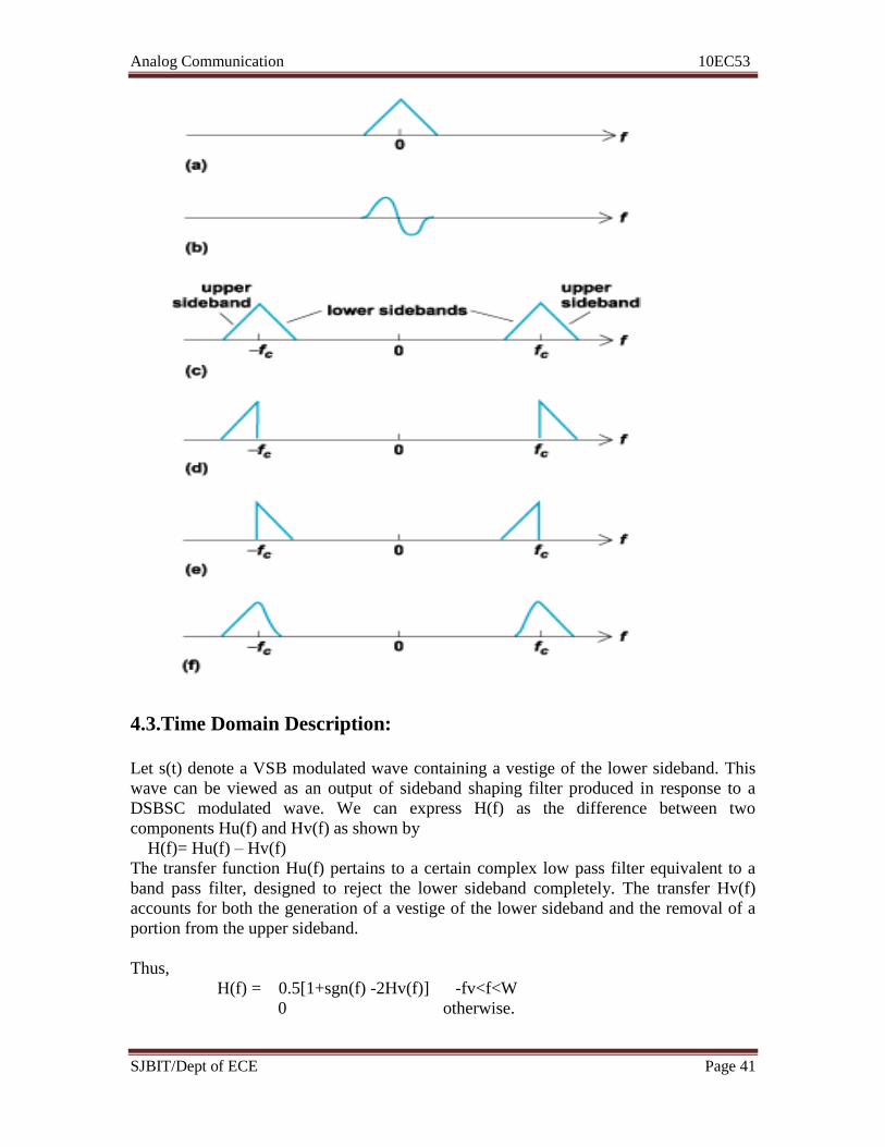
4.3.Time Domain Description:
Let s(t) denote a VSB modulated wave containing a vestige of the lower sideband. This
wave can be viewed as an output of sideband shaping filter produced in response to a
DSBSC modulated wave. We can express H(f) as the difference between two
components Hu(f) and Hv(f) as shown by
H(f)= Hu(f) – Hv(f)
The transfer function Hu(f) pertains to a certain complex low pass filter equivalent to a
band pass filter, designed to reject the lower sideband completely. The transfer Hv(f)
accounts for both the generation of a vestige of the lower sideband and the removal of a
portion from the upper sideband.
Thus,
H(f) = 0.5[1+sgn(f) -2Hv(f)] -fv<f<W
0 otherwise.

Analog Communication 10EC53
SJBIT/Dept of ECE Page 42
Since, both sgn(f) and Hv(f) have purely imaginary inverse fourier transforms, we
introduce a new transfer function
Hq(f) = 1/j[sgn(f) – 2Hv(f)].
The desired representation for a VSB modulated wave containing a vestige of lower
sideband is given as follows : -
s(t)= Ac/2 m(t) cos(2 π fct) – Ac/2 mQ (t)sin(2 π fct).
If the vestigial sideband is increased to the width of a full sideband, the resultant wave
becomes a DSBSC wave and mQ(t) vanishes.
4.4. Envelope Detection of VSB wave plus Carrier:
The modified modulator wave applied to the envelope detector input as
s(t) = Ac[1+0.5kam(t)]cos(2 πfct) – 0.5kaAcmQ(t)sin(2 πfct)
The envelope detector output denoted by a(t) is given as – a(t)= Ac[a+0.5kam(t)]^2 +
[0.5kamQ(t)]^2^0.5
The distortion can be reduced either by reducing the % modulation to reduce ka or by
increasing the width of the vestigial sideband to reduce mQ(t).
4.5.Comparison of Amplitude Modulation Techniques:
In standard AM systems the sidebands are transmitted in full, accompanied by the
carrier. Accordingly, demodulation is accomplished by using an envelope detector
or square law detector. On the other hand in a suppressed carrier system the
receiver is more complex because additional circuitry must be provided for
purpose of carrier recovery.
Suppressed carrier systems require less power to transmit as compared to AM
systems thus making them less expensive.
SSB modulation requires minimum transmitter power and maximum transmission
band with for conveying a signal from one point to other thus SSB modulation is
preferred.
VSB modulation requires a transmission band with that is intermediate then that
of SSB or DSBSC.
DSBSC modulation, SSB modulation, and VSB modulation are examples of
linear modulation. The output of linear modulator can be expressed in the
canonical form given by
s(t)= s1(t)cos(2πfct) –sQ(t) sin(2πfct).
In SSB and VSB modulation schemes the quadrature component is only to
interfere with the in phase component so that power can be eliminated in one of
the sidebands.
The band pass representation can also be used to describe quadrature amplitude
modulation.
The complex envelope of the linearly modulated wave s(t) equals s(t)=s1(t)+jsQ(t).

Analog Communication 10EC53
SJBIT/Dept of ECE Page 43
4.6.Frequency Translations:
4.7. Frequency Division Multiplexing:
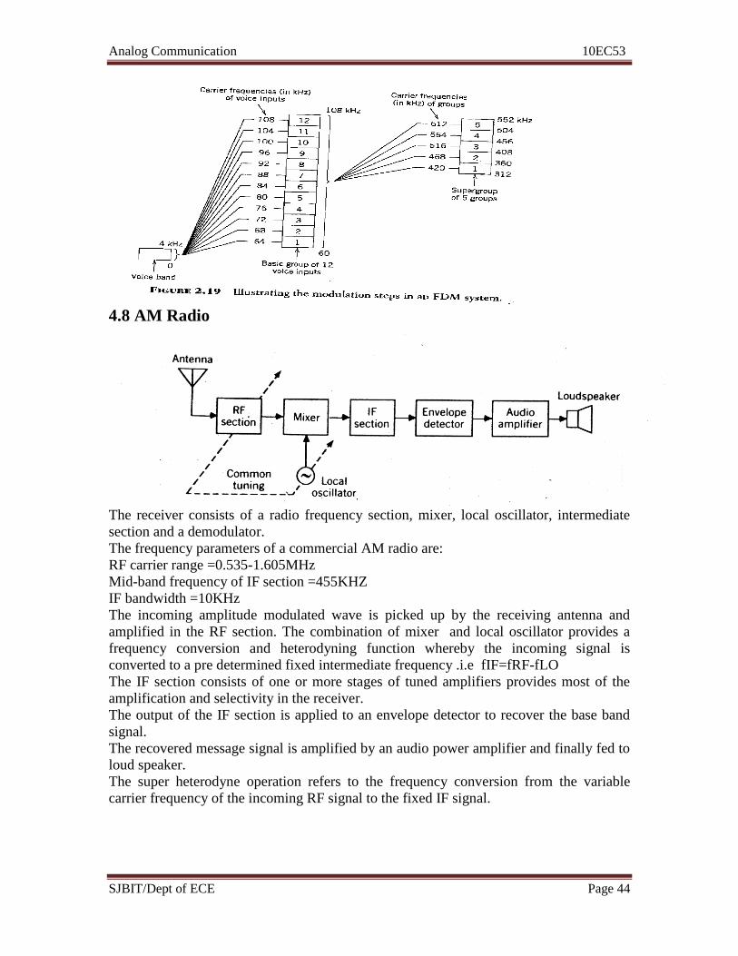
Analog Communication 10EC53
SJBIT/Dept of ECE Page 44
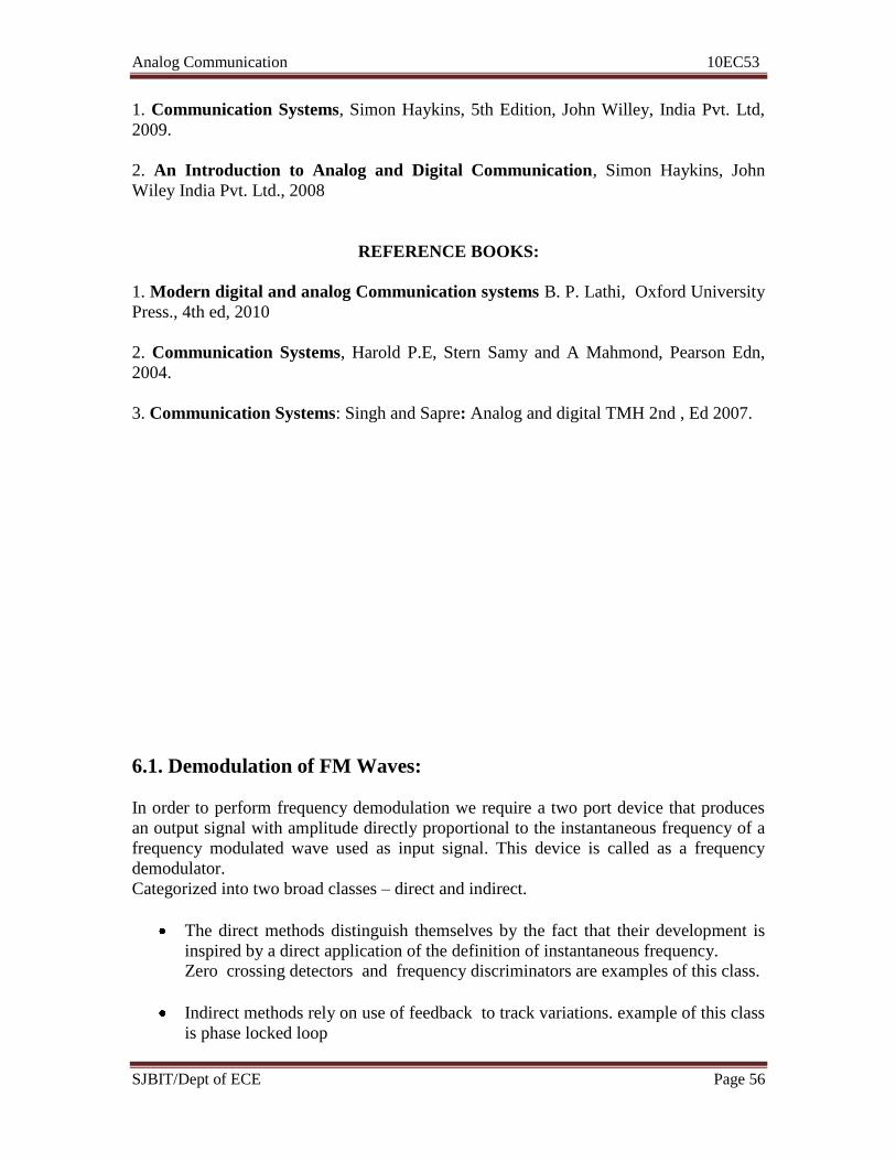
4.8 AM Radio
The receiver consists of a radio frequency section, mixer, local oscillator, intermediate
section and a demodulator.
The frequency parameters of a commercial AM radio are:
RF carrier range =0.535-1.605MHz
Mid-band frequency of IF section =455KHZ
IF bandwidth =10KHz
The incoming amplitude modulated wave is picked up by the receiving antenna and
amplified in the RF section. The combination of mixer and local oscillator provides a
frequency conversion and heterodyning function whereby the incoming signal is
converted to a pre determined fixed intermediate frequency .i.e fIF=fRF-fLO
The IF section consists of one or more stages of tuned amplifiers provides most of the
amplification and selectivity in the receiver.
The output of the IF section is applied to an envelope detector to recover the base band
signal.
The recovered message signal is amplified by an audio power amplifier and finally fed to
loud speaker.
The super heterodyne operation refers to the frequency conversion from the variable
carrier frequency of the incoming RF signal to the fixed IF signal.

Analog Communication 10EC53
SJBIT/Dept of ECE Page 45
Recommended Questions:
1. Explain the scheme for generation & demodulation of VSB waves with relavent
block diagram ?
2. Explain FDM technique?
3. Explain with neat diagram Super heterodyne receiver?
4. Explain Frequnecy TRANSLATION
5. Explain envelope detection of VSBwave+carrier?
6. Define VSB. Explain frequency domain representation of VSB?

Analog Communication 10EC53
SJBIT/Dept of ECE Page 46
UNIT - 5
ANGLE MODULATION (FM)-I
Basic definitions, FM, narrow band FM, wide band FM, transmission bandwidth of FM
waves, generation of FM waves: indirect FM and direct FM. 6 Hrs
TEXT BOOKS:
1. Communication Systems, Simon Haykins, 5th Edition, John Willey, India Pvt. Ltd,
2009.
2. An Introduction to Analog and Digital Communication, Simon Haykins, John
Wiley India Pvt. Ltd., 2008
REFERENCE BOOKS:
1. Modern digital and analog Communication systems B. P. Lathi, Oxford University
Press., 4th ed, 2010
2. Communication Systems, Harold P.E, Stern Samy and A Mahmond, Pearson Edn,
2004.
3. Communication Systems: Singh and Sapre: Analog and digital TMH 2nd , Ed 2007.

Analog Communication 10EC53
SJBIT/Dept of ECE Page 47
5.1. Features of angle modulation:
It can provide a better discrimination (robustness) against noise and interference
than AM
This improvement is achieved at the expense of increased transmission bandwidth
In case of angle modulation, channel bandwidth may be exchanged for improved
noise performance
Such trade-off is not possible with AM.
5.1.1. Basic definitions:
There is yet another way of modulation namely the angle modulation in which the angle
of the carrier wave changes in accordance with the signal
In this method of modulation the amplitude of the carrier wave is maintained constant
The advantage is it can show better discrimination against noise and interference than
amplitude modulation
Let denote the angle of a modulated sinusoidal carrier
Where is the carrier amplitude. A complete oscillation occurs whenever changes
by radians. If increases monotonically with time the average frequency in Hertz,
over an interval from t to Δt
We may thus define the instantaneous frequency of the angle-modulated signal s(t)
The angle modulated signal s(t) as a rotating phasor of length Ac and angle
In simple case of unmodulated carrier the angle is
And the corresponding phasor rotates with a constant angular velocity equal to
There are infinite numbers of ways in which the angle may be varied in some
manner with the message signal. We consider only two methods phase modulation and
frequency modulation
5.2. Phase Modulation:

Analog Communication 10EC53
SJBIT/Dept of ECE Page 48
Phase modulation is that form of angle modulation in which the angle is varied
linearly with the message signal m(t)
The term 2 represents the angle of the unmodulated carrier wave and constant Kp is
the phase sensitivity of the modulator expressed in radian per volt
We have assumed that the angle of the unmodulated carrier is zero at time t =0
The phase –modulated signal s(t) is thud described in the time domain by
5.3. FREQUENCY MODULATION :
Frequency modulation is that form of angle modulation in which the instantaneous
frequency if(t) is varied linearly with the message signal m(t)
]
Frequency of the carrier varies with the signal mathematically in the above equation

Analog Communication 10EC53
SJBIT/Dept of ECE Page 49
Comparison between phase and frequency modulated equations frequency modulated
signal is the same as phase modulation with the message signal integrated
The variation of the frequency is discrete differing from the sinusoidal modulated wave
where the frequency changes constantly
There will be a phase discontinuity in case of phase modulation when message is a square
wave
There is a phase reversal in the phase modulation
The visualization is easier
Note: The FM wave is a non linear function of the modulating wave m(t)
5.4. SINGLE TONE FREQUENCY MODULATION
Consider a single tone sinusoidal modulating wave
The instantaneous frequency is

Analog Communication 10EC53
SJBIT/Dept of ECE Page 50
Where
Is called frequency deviation representing maximum departure of the instantaneous
frequency from the carrier
The fundamental characteristics of an FM is that the frequency deviation is directly
proportional to the amplitude of the base band signal and is independent of the
modulation frequency
Instantaneous angle is given by
The modulation index of FM wave is given by
5.5. SPECTRUM ANALYSIS OF SINUSOIDAL FM WAVE
We can express this as in phase and quadrature components
Hence the complex envelope equals +
And the FM signal is given by
The complex envelope is a periodic sequence of time with the fundamental frequency
equal to modulation frequency, we may therefore expand s`(t) in the form of a complex
Fourier series as follows
Where the complex Fourier co-efficient equals
The integral on the right hand side is recognized as Bessel function of nth order and first
kind and argument β, this function is commonly denoted by the symbol Jn(β)
Hence we can write

Analog Communication 10EC53
SJBIT/Dept of ECE Page 51
On evaluation we get
Taking Fourier transform we obtain a discrete spectrum on both sides
The plots of Bessel function shows us that for a fixed n alternates between positive
and negative values for increasing and approaches infinity. Note that for a
fixed value of
We only need the positive values hence those are considered
The following are the properties of FM waves
PROPERTY 1:
For small values of the modulation index compared to one radian, the FM wave
assumes a narrow band form and consisting essentially of a carrier, an upper side
frequency and a lower side frequency component
This property follows from the fact that for small values of we have
These are the approximations assumed for
The FM wave can be approximated as a sum of carrier an upper side frequency of
amplitude and a lower side frequency component and phase shift equals to 180
PROPERTY 2:
For large values of modulation index compared to one radian the FM contains a carrier
and an infinite number of side bands on either side located symmetrically around the
carrier
Note that the amplitude of the carrier component in a wide band FM wave varies with the
modulation index in accordance with
PROPERTY 3:
The envelope of an FM wave is constant so that the average power of such a wave
dissipated in 1Ω resistor is also a constant
The average power is equal to the power of the carrier component it is given by
The average power of a single tone FM wave s(t) may be expressed in the form of a
corresponding series as

Analog Communication 10EC53
SJBIT/Dept of ECE Page 52
5.6. Generation of fm waves:
There are two types
Direct method and indirect method
In the indirect method of producing a narrow band FM is generated then frequency
multiplied to obtain wide band frequency modulated wave
5.6.1. INDIRECT METHOD:
FM modulation : The amplitude of the modulated carrier is held constant and the time
derivative of the phase of the carrier is varied linearly with the information signal.
Hence
tdt
tdt cc
ci
)()(
)()( tvkt mfc
)()( tvkt mfci

Analog Communication 10EC53
SJBIT/Dept of ECE Page 53
The angle of the FM signal can be obtained by integrating the instantaneous frequency.
Notes:
vm(t) is a sinusoidal signal, hence:
Therefore
For NBFM
therefore
Hence
Summary:
Therefore NBFM signal can be generated using phase modulator circuit as shown.
t
mfc dttvkt0
)()(
1)(tc
1)](cos[ tc )()](sin[ tt cc
ttdttt cc
t
ic
0
)()(
t
mfc
t
mfcc
dttvkt
dttvkt
0
0
)(
)()(
)sin(
)sin(
)cos()(0
t
tEk
dttEkt
m
m
m
mf
t
mmfc
1)sin( tm
1)()(0
t
mfc dttvkt
)](sin[)(sin)](cos[)(cos
)]([cos)(
ttEttE
ttEtv
cccccc
cccFM
)(sin)()(cos)( tEttEtv cccccNBFM

Analog Communication 10EC53
SJBIT/Dept of ECE Page 54
To obtain WBFM signal, the output of the modulator circuit (NBFM) is fed into
frequency multiplier circuit and the mixer circuit.
The function of the frequency multiplier is to increase the frequency deviation or
modulation index so that WBFM can be generated.
The instantaneous value of the carrier frequency is increased by N times.
Output of the frequency multiplier :
Where
And
Where
It is proven that the modulation index was increased by N times following this equation.
The output equation of the frequency multiplier :
Pass the signal through the mixer, then WBFM signal is obtained :
BPF is used to filter the WBFM signal desired either at ωc2+ ωLO or at ωc2- ωLO .
Hence the output equation
Recommended Questions:
1. Explain with suitable functional diagram of generation of WBFM from NBFM?
2. Derive an expression for FM wave?
3. Define modulation index, maximum deviation and BW of an FM wave?
cc N2
cc N2
)()()( 1 ttt cci
)(
)]([
)()(
2
12
tN
tN
tNt
cc
cc
)sin(
)sin(
)cos()(0
t
tEk
dttEkt
m
m
m
mf
t
mmfc
12 N
)]([
)]([cos)(
2
2
tNtkosE
tEtv
ccc
cFM
)]()cos[()]()cos[(
)cos(2 x )]([cos)(
22
2
tNtEtNtE
ttNtEtv
cLOcccLOcc
LOcccFM
)]()[(
)]()[()(
2
2
tNtkosE
tNtkosEtv
cLOcc
cLOcc
WBFM

Analog Communication 10EC53
SJBIT/Dept of ECE Page 55
4. Derive an expression for single tone FM?
5. Show that A NBFM and AM systems have same BW?
6. Differentiate between NBFM & WBFM?
7. Differentiate between NBFM & AM?
UNIT - 6
ANGLE MODULATION (FM)-II
Demodulation of FM waves, FM stereo multiplexing, Phase-locked loop, Nonlinear
model of the phase – locked loop, Linear model of the phase – locked loop, Nonlinear
effects in FM systems. 7 Hrs
TEXT BOOKS:
Analog Communication 10EC53
SJBIT/Dept of ECE Page 56
1. Communication Systems, Simon Haykins, 5th Edition, John Willey, India Pvt. Ltd,
2009.
2. An Introduction to Analog and Digital Communication, Simon Haykins, John
Wiley India Pvt. Ltd., 2008
REFERENCE BOOKS:
1. Modern digital and analog Communication systems B. P. Lathi, Oxford University
Press., 4th ed, 2010
2. Communication Systems, Harold P.E, Stern Samy and A Mahmond, Pearson Edn,
2004.
3. Communication Systems: Singh and Sapre: Analog and digital TMH 2nd , Ed 2007.
6.1. Demodulation of FM Waves:
In order to perform frequency demodulation we require a two port device that produces
an output signal with amplitude directly proportional to the instantaneous frequency of a
frequency modulated wave used as input signal. This device is called as a frequency
demodulator.
Categorized into two broad classes – direct and indirect.
The direct methods distinguish themselves by the fact that their development is
inspired by a direct application of the definition of instantaneous frequency.
Zero crossing detectors and frequency discriminators are examples of this class.
Indirect methods rely on use of feedback to track variations. example of this class
is phase locked loop

Analog Communication 10EC53
SJBIT/Dept of ECE Page 57
6.2. Balanced Frequency Discriminator:
Ideal slope circuit is characterized by an imaginary transfer function, varying linearly
with frequency inside a prescribed interval.
For evaluation of s1(t) we replace the slope circuit with an equivalent low pass filter and
driving this filter with a complex envelope of the input FM wave s(t).
H1(f-fc)=H1(f) provided f>0.
The ideal frequency discriminator is a pair of slope circuits with a complex transfer
function followed by envelope detector and summer. This scheme is called a balanced
frequency discriminator or back to back frequency discriminator
6.3. Phase locked loop:
The PLL is a negative feedback system that consists of a multiplier, a loop filter and a
VCO connected in the form of a feed back loop.
The VCO is a sine wave generator whose frequency is determined by a voltage applied to
it from an external source.
Initially we have adjusted the VCO so that when the control voltage is zero two
conditions are satisfied The frequency of the VCO is set at unmodulated carrier
frequency fc. The VCO output has a 90 phase shift wrt the unmodulated carrier wave.
The incoming fm wave s(t) and the VCO output r(t) are applied to the multiplier
producing two components
A frequency component represented as kmAcAvsin[4πfct+ф1(t)+ф2(t)].
A low frequency component represented by kmAcAvsin[ф1(t)-ф2(t)]. where km is a
multiplier gain measured in 1/volt. The high frequency component is eliminated by the
Analog Communication 10EC53
SJBIT/Dept of ECE Page 58
low pass action of the filter and the VCO. Thus the input to the loop filter is given by
e(t)=kmAcAv sin[фc(t)].
Here фc(t) is the phase error.
Linearized model: When the phase error is zero the phase locked loop is said to be in phase lock. When the
phase error is at times small compared with one radian we use the approximation
sin[фc(t)]= фc(t).
We represent phase locked loop by a linearized model according to which phase error is
related to input phase by a integro differential equation.
L (f)=Ko(H(f)/jf)
H(f) is a transfer function of loop filter and L(f) is the open loop transfer function of
phase locked loop. Provided the magnitude of L(f) is very large for all frequencies , the
phase locked loop is seen as a differentiator with output scaled by 1/2πkv.
The output V(t) of the phase locked loop is almost the same except for the scale factor
kf/kv as m(t)and the frequency demodulation is accomplished. The bandwidth of
incoming fm wave is much wider than that of the loop filter is characterised by H(f).
For a pll H(f)=1.

Analog Communication 10EC53
SJBIT/Dept of ECE Page 59
Nonlinear model of a PLL b) Linear model c) simplified model
First Order Phase Locked Loop: At H(f)=1 the linearised model of the loop becomes фc(f)=ф1(f)/1+Ko/jf
Assuming a single tone modulating wave m(t)=Amcos(2πfmt) and then simplifying we
get
фe(t)=фeocos(2πfmt+ψ)
ψ=-1/(tan fm/Ko).
The amplitude Ao is defined as [Δf/kv]/[1+(fm/Ko)^2]^(0.5).
sin ф=δf/ka.
6.4. FM Radio: As with standard AM radio, most FM radio receivers are of super-heterodyne type.
Typical parameters of commercial fm radio are –
RF carrier wave=88-108 Mhz
Midband frequency of IF section = 10.7 Mhz
IF Bandwidth = 200kHz

Analog Communication 10EC53
SJBIT/Dept of ECE Page 60
In FM radio modifications are made to degrade effects of noise –
1. A de-emphasis n/w is added to the audio power amplifier so as to compensate for the
use of pre-emphasis n/w at the transmitter.
2. A post detection filter, labeled “baseband lowpass filter” is added at the o/p end of the
receiver
6.5. FM stereo multiplexing:
Stereo multiplexing is a form of frequency division multiplexing designed to transmit two
separate signals via the same carrier. It is widely used in the FM radio broadcasting to
send two different elements of a program. For example the different elements can be
sections of orchestra, a vocalist and an accompanist. This gives a spatial dimension to its
perception for the listener at the receiving end.
The two important factors that influence the FM stereo transmission are:
1. The transmission has to operate within the allocated FM broadcast channels.
2. It has to compatible with the monophonic receivers.
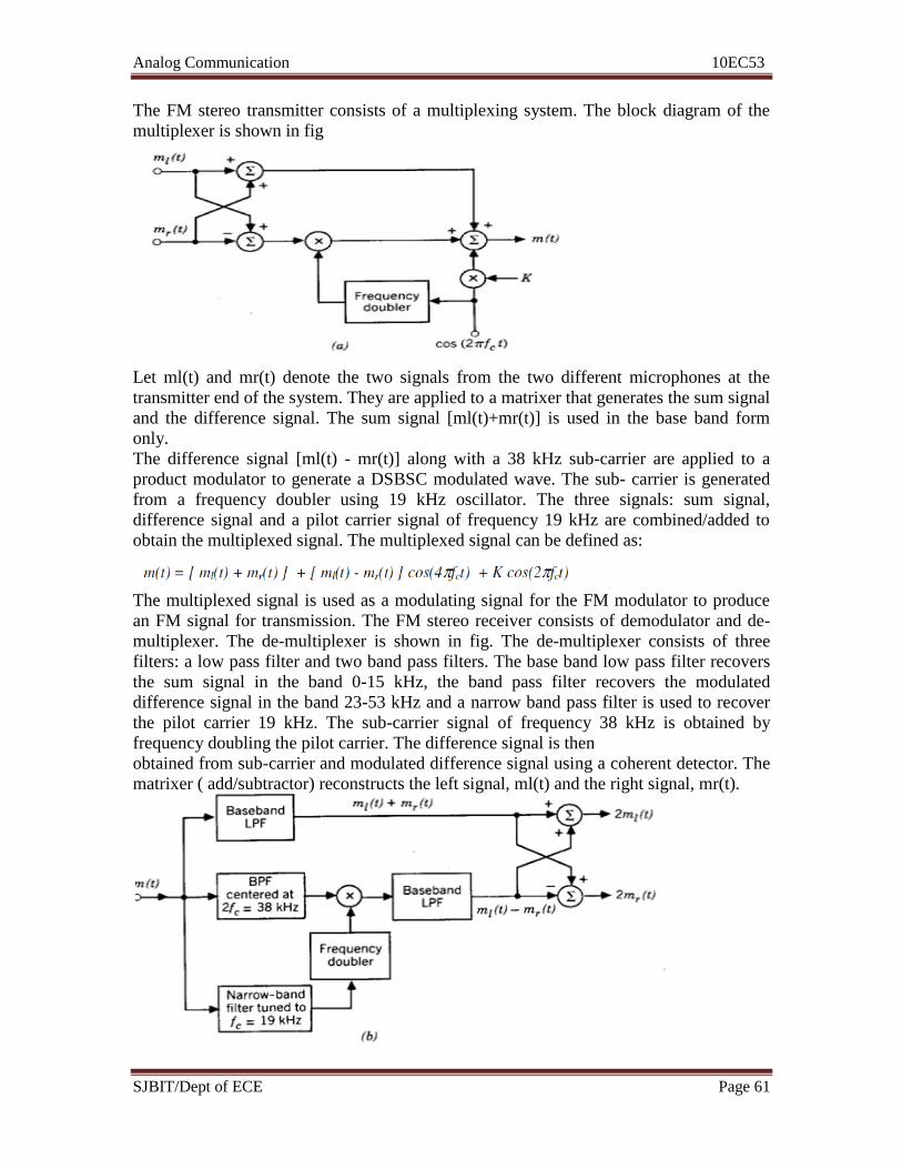
Analog Communication 10EC53
SJBIT/Dept of ECE Page 61
The FM stereo transmitter consists of a multiplexing system. The block diagram of the
multiplexer is shown in fig
Let ml(t) and mr(t) denote the two signals from the two different microphones at the
transmitter end of the system. They are applied to a matrixer that generates the sum signal
and the difference signal. The sum signal [ml(t)+mr(t)] is used in the base band form
only.
The difference signal [ml(t) - mr(t)] along with a 38 kHz sub-carrier are applied to a
product modulator to generate a DSBSC modulated wave. The sub- carrier is generated
from a frequency doubler using 19 kHz oscillator. The three signals: sum signal,
difference signal and a pilot carrier signal of frequency 19 kHz are combined/added to
obtain the multiplexed signal. The multiplexed signal can be defined as:
The multiplexed signal is used as a modulating signal for the FM modulator to produce
an FM signal for transmission. The FM stereo receiver consists of demodulator and de-
multiplexer. The de-multiplexer is shown in fig. The de-multiplexer consists of three
filters: a low pass filter and two band pass filters. The base band low pass filter recovers
the sum signal in the band 0-15 kHz, the band pass filter recovers the modulated
difference signal in the band 23-53 kHz and a narrow band pass filter is used to recover
the pilot carrier 19 kHz. The sub-carrier signal of frequency 38 kHz is obtained by
frequency doubling the pilot carrier. The difference signal is then
obtained from sub-carrier and modulated difference signal using a coherent detector. The
matrixer ( add/subtractor) reconstructs the left signal, ml(t) and the right signal, mr(t).

Analog Communication 10EC53
SJBIT/Dept of ECE Page 62
6.6 Zero crossing detector
This detector circuit exploits the property that the instantaneous frequency of an FM
wave is approximately given by
where Δt is the time difference between the adjacent zero crossings of the FM wave. Let
n0 be the number of zero crossings inside an interval T and then express the time Δt is
given by
Thus the instantaneous frequency is linearly related to the message signal m(t); it can be
recovered from the knowledge of n0.
A simplified block diagram of a zero crossing detector based on the above principle is
shown in the fig. The basic blocks are Limiter, Pulse generator and Integrator. The
Limiter produces a square wave version of the input FM wave. The Pulse generator
produces pulses at the positive going edges and negative going edges of the limiter
output. The Integrator performs the averaging over the interval T and hence produces the
message signal.
Recommended Questions:
1. Explain FM sterio multiplexing?
2. Using PLL obtain Linear and non linear model?
3. Explain Direct method of generation of FM?
4. Derive an expression for instantaneous frequency of FM for sinusoidal
modulation/
5. Explain Balanced frequency descriminator?
6. Explain non linearity & its effects in FM?
7. Explain FM detection using PLL?

Analog Communication 10EC53
SJBIT/Dept of ECE Page 63
UNIT – 7
NOISE
Introduction, shot noise, thermal noise, white noise, Noise equivalent bandwidth, Narrow
bandwidth, Noise Figure, Equivalent noise temperature, cascade connection of two-port
networks. 6 Hrs
TEXT BOOKS:
1. Communication Systems, Simon Haykins, 5th Edition, John Willey, India Pvt. Ltd,
2009.
2. An Introduction to Analog and Digital Communication, Simon Haykins, John
Wiley India Pvt. Ltd., 2008
REFERENCE BOOKS:
1. Modern digital and analog Communication systems B. P. Lathi, Oxford University
Press., 4th ed, 2010
2. Communication Systems, Harold P.E, Stern Samy and A Mahmond, Pearson Edn,
2004.
3. Communication Systems: Singh and Sapre: Analog and digital TMH 2nd , Ed 2007.

Analog Communication 10EC53
SJBIT/Dept of ECE Page 64
7.1. Introduction
Electronic noise is a random fluctuation in an electrical signal, a characteristic of all
electronic circuits. Noise generated by electronic devices varies greatly, as it can be
produced by several different effects. Thermal noise is unavoidable at non-zero
temperature .while other types depend mostly on device type (such as shot noise, which
needs steep potential barrier) or manufacturing quality and semiconductor defects (such
as conductance fluctuations, including 1/f noise).
In communication systems, the noise is an error or undesired random disturbance of a
useful information signal, introduced before or after the detector and decoder. The noise
is a summation of unwanted or disturbing energy from natural and sometimes man-made
sources. Noise is, however, typically distinguished from interference, (e.g. cross-talk,
deliberate jamming or other unwanted electromagnetic interference from specific
transmitters), for example in the signal-to-noise ratio (SNR), signal-to-interference ratio
(SIR) and signal-to-noise plus interference ratio (SNIR) measures. Noise is also typically
distinguished from distortion, which is an unwanted alteration of the signal waveform, for
example in the signal-to-noise and distortion ratio (SINAD). In a carrier-modulated
passband analog communication system, a certain carrier-to-noise ratio (CNR) at the
radio receiver input would result in a certain signal-to-noise ratio in the detected message
signal. In a digital communications system, a certain Eb/N0 (normalized signal-to-noise
ratio) would result in a certain bit error rate (BER).
While noise is generally unwanted, it can serve a useful purpose in some applications,
such as random number generation or dithering.
7.2. Types of noise:
Thermal noise: Johnson–Nyquist noise (sometimes thermal, Johnson or Nyquist noise) is unavoidable,
and generated by the random thermal motion of charge carriers (usually electrons), inside
an electrical conductor, which happens regardless of any applied voltage.
Thermal noise is approximately white, meaning that its power spectral density is nearly
equal throughout the frequency spectrum. The amplitude of the signal has very nearly a
Gaussian probability density function. A communication system affected by thermal
noise is often modeled as an additive white Gaussian noise (AWGN) channel.
As the amount of thermal noise generated depends upon the temperature of the circuit,
very sensitive circuits such as preamplifiers in radio telescopes are sometimes cooled in
liquid nitrogen to reduce the noise level.
Shot noise Shot noise in electronic devices consists of unavoidable random statistical fluctuations of
the electric current in an electrical conductor. Random fluctuations are inherent when
current flows, as the current is a flow of discrete charges (electrons).
Flicker noise Flicker noise, also known as 1/f noise, is a signal or process with a frequency spectrum
that falls off steadily into the higher frequencies, with a pink spectrum. It occurs in

Analog Communication 10EC53
SJBIT/Dept of ECE Page 65
almost all electronic devices, and results from a variety of effects, though always related
to a direct current.
Burst noise Burst noise consists of sudden step-like transitions between two or more levels (non-
Gaussian), as high as several hundred millivolts, at random and unpredictable times. Each
shift in offset voltage or current lasts for several milliseconds, and the intervals between
pulses tend to be in the audio range (less than 100 Hz), leading to the term popcorn noise
for the popping or crackling sounds it produces in audio circuits.
Avalanche noise Avalanche noise is the noise produced when a junction diode is operated at the onset of
avalanche breakdown, a semiconductor junction phenomenon in which carriers in a high
voltage gradient develop sufficient energy to dislodge additional carriers through physical
impact, creating ragged current flows.
7.3. Quantification The noise level in an electronic system is typically measured as an electrical power N in
watts or dBm, a root mean square (RMS) voltage (identical to the noise standard
deviation) in volts, dBμV or a mean squared error (MSE) in volts squared. Noise may
also be characterized by its probability distribution and noise spectral density N0(f) in
watts per hertz.
A noise signal is typically considered as a linear addition to a useful information signal.
Typical signal quality measures involving noise are signal-to-noise ratio (SNR or S/N),
signal-to-quantization noise ratio (SQNR) in analog-to-digital coversion and
compression, peak signal-to-noise ratio (PSNR) in image and video coding, Eb/N0 in
digital transmission, carrier to noise ratio (CNR) before the detector in carrier-modulated
systems, and noise figure in cascaded amplifiers.
Noise is a random process, characterized by stochastic properties such as its variance,
distribution, and spectral density. The spectral distribution of noise can vary with
frequency, so its power density is measured in watts per hertz (W/Hz). Since the power in
a resistive element is proportional to the square of the voltage across it, noise voltage
(density) can be described by taking the square root of the noise power density, resulting
in volts per root hertz (). Integrated circuit devices, such as operational amplifiers
commonly quote equivalent input noise level in these terms (at room temperature).
Noise power is measured in Watts or decibels (dB) relative to a standard power, usually
indicated by adding a suffix after dB. Examples of electrical noise-level measurement
units are dBu, dBm0, dBrn, dBrnC, and dBrn(f1 − f2), dBrn(144-line).
Noise levels are usually viewed in opposition to signal levels and so are often seen as part
of a signal-to-noise ratio (SNR). Telecommunication systems strive to increase the ratio
of signal level to noise level in order to effectively transmit data. In practice, if the
transmitted signal falls below the level of the noise (often designated as the noise floor)
in the system, data can no longer be decoded at the receiver. Noise in telecommunication
systems is a product of both internal and external sources to the system.
Analog Communication 10EC53
SJBIT/Dept of ECE Page 66
7.4. Dither If the noise source is correlated with the signal, such as in the case of quantisation error,
the intentional introduction of additional noise, called dither, can reduce overall noise in
the bandwidth of interest. This technique allows retrieval of signals below the nominal
detection threshold of an instrument. This is an example of stochastic resonance.
7.5. Noise figure (NF) It is a measure of degradation of the signal-to-noise ratio (SNR), caused by components
in a radio frequency (RF) signal chain. The noise figure is defined as the ratio of the
output noise power of a device to the portion thereof attributable to thermal noise in the
input termination at standard noise temperature T0 (usually 290 K). The noise figure is
thus the ratio of actual output noise to that which would remain if the device itself did not
introduce noise. It is a number by which the performance of a radio receiver can be
specified.
The noise figure is the difference in decibels (dB) between the noise output of the actual
receiver to the noise output of an “ideal” receiver with the same overall gain and
bandwidth when the receivers are connected to matched sources at the standard noise
temperature T0 (usually 290 K). The noise power from a simple load is equal to kTB,
where k is Boltzmann's constant, T is the absolute temperature of the load (for example a
resistor), and B is the measurement bandwidth.
This makes the noise figure a useful figure of merit for terrestrial systems where the
antenna effective temperature is usually near the standard 290 K. In this case, one
receiver with a noise figure say 2 dB better than another, will have an output signal to
noise ratio that is about 2 dB better than the other. However, in the case of satellite
communications systems, where the antenna is pointed out into cold space, the antenna
effective temperature is often colder than 290 K. In these cases a 2 dB improvement in
receiver noise figure will result in more than a 2 dB improvement in the output signal to
noise ratio. For this reason, the related figure of effective noise temperature is therefore
often used instead of the noise figure for characterizing satellite-communication receivers
and low noise amplifiers.
7.6. Noise Temperature: In heterodyne systems, output noise power includes spurious contributions from image-
frequency transformation, but the portion attributable to thermal noise in the input
termination at standard noise temperature includes only that which appears in the output
via the principal frequency transformation of the system and excludes that which appears
via the image frequency transformation.
In electronics, noise temperature is one way of expressing the level of available noise
power introduced by a component or source. The power spectral density of the noise is
expressed in terms of the temperature (in kelvins) that would produce that level of
Johnson–Nyquist noise
Thus the noise temperature is proportional to the power spectral density of the noise, P /
B. That is the power that would be absorbed from the component or source by a matched
load. Noise temperature is generally a function of frequency, unlike that of an ideal
resistor which is simply equal to the actual temperture of the resistor at all frequencies.

Analog Communication 10EC53
SJBIT/Dept of ECE Page 67
Recommended Questions:
1. What is Noise?
2. Define Noise figure and noise factor?
3. Derive the expression for noise equivalent bandwidth?
4. Define Shot noise & Thermal Noise?
5. Derive relation between noise figure and eq noise temperature?
6. Define noise equivalent bandwidth?
7. Explain noise figure measurement?

Analog Communication 10EC53
SJBIT/Dept of ECE Page 68
UNIT - 8
NOISE IN CONTINUOUS WAVE MODULATION SYSTEMS
Introduction, Receiver model, Noise in DSB-SC receivers, Noise in SSB receivers, Noise
in AM receivers, Threshold effect, Noise in FM receivers, FM threshold effect, Pre-
emphasis and De-emphasis in FM 7 Hrs
TEXT BOOKS:
1. Communication Systems, Simon Haykins, 5th Edition, John Willey, India Pvt. Ltd,
2009.
2. An Introduction to Analog and Digital Communication, Simon Haykins, John
Wiley India Pvt. Ltd., 2008
REFERENCE BOOKS:
1. Modern digital and analog Communication systems B. P. Lathi, Oxford University
Press., 4th ed, 2010
2. Communication Systems, Harold P.E, Stern Samy and A Mahmond, Pearson Edn,
2004.
3. Communication Systems: Singh and Sapre: Analog and digital TMH 2nd , Ed 2007.

Analog Communication 10EC53
SJBIT/Dept of ECE Page 69
8.1. Channel and Receiver Model:
Channel and receiver model.
Channel: additive white Gaussian noise(AWGN)
Receiver: a BPF followed by a demodulator
8.1.1 Signal-to-Noise Ratios (SNR):
Let s(t) be the modulated signal, and let w(t) be the AWGN channel noise with PSD of
N0/2. The output of the BPF is
x(t) = s(t) + n(t),
where n(t) can be expressed as n(t) = nI (t) cos(2πfct) − nQ(t) sin(2πfct).
8.2 Coherent Linear Receivers:
Consider the linear DSB-SC modulation scheme with coherent detection

Analog Communication 10EC53
SJBIT/Dept of ECE Page 70
Coherent DSB-SC demodulator.
The DSB-SC signal is
s(t) = Ac cos(2πfct)m(t).
Assume m(t) is an RP bandlimited to a maximum frequency W.
Also assume the carrier signal is an RP (due to a random phase) and independent of m(t).
The PSD of s(t) is
The PSD of w(t) is N0/2. The average noise power over the message BW is WN0 note
that the message signal occupies the frequency band from −W to W).
The channel SNR is
8.3. Envelope Detector:
Consider an AM receiver with envelope detection:
Recall an AM signal is given by

Analog Communication 10EC53
SJBIT/Dept of ECE Page 71
The message BW is W= average noise
Power within BW = WNo=
8.4 Pre-emphasis and De-emphasis:
In common narrowband two way fm communications, Pre emphasis follows a 6 dB per
octave rate. This means that as the frequency doubles, the amplitude increases 6 dB. This
is usually done between 300 - 3000 cycles. Pre emphasis is needed in FM to maintain
good signal to noise ratio. Why is it necessary? Common voice characteristics emit low

Analog Communication 10EC53
SJBIT/Dept of ECE Page 72
frequencies higher in amplitude than high frequencies. The limiter circuits that clip the
voice to allow protection of over deviation are usually not frequency sensitive, and are
fixed in level, so they will clip or limit the lows before the highs. This results in added
distortion because of the lows overdriving the limiter. Pre emphasis is used to shape the
voice signals to create a more equal amplitude of lows and highs before their application
to the limiter. The result is that the signal received is perceived louder due to more equal
clipping or limiting of the signal, but probably more important is the increased level of
the higher frequencies being applied to the modulator results in a better transmitted audio
signal to noise ratio due to the highs being above the noise as much or more than the
lows.
Transmitters that employ a true FM modulator require a pre emphasis circuit before the
modulator fore the true FM modulator doesn't automatically pre emphasize the audio like
a transmitter that uses a phase modulator. A separate circuit is not necessary for pre
emphasis in a transmitter that has a phase modulator because the phase modulator applies
pre emphasis to the transmitted audio as a function of the phase modulator.
The receiver De emphasis circuitry takes the unnatural sounding pre emphasized audio
and turns it back into its original response. Pre emphasized (discriminator) audio is
however available directly from the audio demodulation (discriminator) circuitry.
In linking systems, many choose to eliminate the emphasis circuitry to allow better
representation of retransmitted signals. Since the signal has already been pre emphasized
(by the user that is transmitting,) and since the receiver you are listening to takes care of
the de emphasis.... it doesn't need to be done over and over again.
Some loss of quality does exist, but quality is better maintained by a flat system. A flat
audio response system is one which has equal output deviation for the same input
deviation, no matter what the applied audio frequency is within reason. Reasonable audio
frequency response would be from 50 cycles to about 3500 to 5000 cycles in a system not
filtering PL. Audio response in a system filtering PL would be around 250 to about 3500
to 5000 cycles. Upper cut off frequency would be determined mainly on acceptable use
of available bandwidth.
Injecting discriminator audio back into an FM modulator without any limiting or low
pass filtering is bad news, plain and simple. On UHF, you've probably been able to get
away with it without excessively bothering either of your adjacent channel neighbors, but
on 2m, especially with 15 kHz spacing, you'd be asking for a lynching.
Without low pass filtering, all of the high frequency energy (hiss) that comes from the
discriminator from a noisy user, if not low pass filtered, will deviate your transmitter in
excess of 5 kHz, in addition to pushing the sidebands out further than they would be if the
AF was cut off at/about 3 kHz. Do this to see what I mean. Set your repeater up for 1:1
input to output ratio (like, put in a signal that is deviated 3 kHz by a 1 kHz tone, and set
your Tx audio gain to get 3 kHz out of the transmitter). Now open your repeater receiver
squelch wide open. You should see your transmitter is now deviating somewhere around
8 or 9 kHz (presuming you have enough audio headroom through the controller). Under
this test condition, the combination of the excessive deviation and the lack of high
frequency filtering will make your signal somewhere around 30 kHz wide instead of 16
as it should be. The only thing "limiting" the occupied bandwidth at that point is the

Analog Communication 10EC53
SJBIT/Dept of ECE Page 73
dynamic range of the audio circuits and the natural high frequency rolloff of the
discriminator's output noise. Look at it on a spectrum analyzer if you don't believe me.
Obviously that's a worst case scenario, but the fact remains that you should have brick
wall limiting at 5 kHz (a little lower at 15 kHz channel spacing), and low pass filtering at
3 kHz (a little higher if you want on 25 kHz channels).
A repeater can be built to utilize a flat audio response to maintain quality through the
system. This is fairly easy in a system using a true FM modulator. Usually modification
to the controller is necessary to allow it, especially ones that have speech or a phone
patch. Systems using a phase modulator require de emphasis before the modulator
because of the automatic pre emphasis of the phase modulator, and for this reason... it is
easier to utilize flat audio modifications and maintain quality audio in a system
employing a true FM modulator in the transmitter.
Recommended Questions:
1. Derive the expression for o/p SNR of an AM receiver using an envelope
detector?
2. Explain Capture effect and Threshold effect?
3. Explain Pre-emphasis?
4. Explain De-emphasis?
5. Derive the expression for o/p SNR of an FM receiver using coherent detector?
6. Derive the expression for FOM of DSB-SCreceiver using coherent detector?