ece 8700, communication systems engineering, spring 2011 course information
TRANSCRIPT

ECE 8700, Communication Systems Engineering, Spring 2011Course Information (Draft: 12/29/10)
Instructor: Kevin Buckley, Tolentine 433a, 610-519-5658 (Office), 610-519-4436 (Fax),610-519-5864 (CEER307), [email protected], www.ece.villanova.edu/user/buckley
Office Hours:* Mon. 11:30am-12:30pm (T433a); Wed. 11:30am-12:30pm (T433a); Thurs. 1-2pm (T433a);Fri. 9:30-10:30am (T433a)
* by appointment, or stop in any time I’m available
Prerequisites: Undergraduate background in engineering probability and statistics, and inprinciples of communications (equivalent to ECE 3720 and ECE 3770).
Grading Policy:* Homework: due before class about every other week - 20%* Three Computer Assignments - 10% each* Test 1: Wed. 2/23 (Chapts. 1-3 of Course Notes), 2 hrs. in class - 25 %* Test 2: Finals Week (Chapts. 4-7 of Course Notes), 2 hrs. in class - 25 %
Text: Digital Communications, 5-th edition, by John Proakis & Masoud Salehi, McGraw-Hill, 2008. ISBN: 978-0-07-295716-6.
Course Notes will be provided. Primarily, you will be responsible for the material in theCourse Notes. The Text will be used extensively as a reference, so you will be responsiblefor specific Sections of the Text which will be identified.
Reference:
• Introduction to Analog and Digital Communications, 2-nd edition, by Simon Haykin& Michael Moher, Wiley & Sons, 2007.
• Signals & Systems 2-nd ed., Alan Oppenheim & Alan Willsky, Prentice-Hall, 1997.
• Linear Algebra and Its Applications, 3-rd ed., by Gilbert Strang, Harcourt Brace Jo-vanovich, 1976.
• Probability, Random Variables, and Random Signal Principles, 4-th ed., by PaytonPeebles, McGraw Hill, 2001.
Course Description: This course covers basic topics in digital communications. Topicscovered in-depth include: modulation schemes, maximum likelihood detection, maximumlikelihood sequence estimation, the Viterbi algorithm, carrier and symbol synchronization,bandlimited channels, intersymbol interference modeling, and optimum channel equaliza-tion. We also briefly overview: adaptive equalization; information theory & coding; fadingchannels, MIMO systems and space-time coding; multicarrier and spread spectrum commu-nications; and multiuser communications.
1

ECE 8700, Communication Systems Engineering, Spring 2010Homework, Computer Assignment & Text Policies
Submission of Homeworks (HWs) & Computer Assignments (CAs):
Distance education students can submit HWs and CAs by Fax (610-519-4436) or email([email protected]). For Fax submissions, only one transmission is accepted perassignment. For emails, only one file will be accepted per assignment, and that file can beonly a .pdf or .doc file (e.g. not .zip or .docx files).
Assignments are due by the beginning of class on the date indicated on the assignment(i.e. on a Wednesday), however they will not be considered late if submitted by midnightthat day. If submitted between midnight and 5pm the next day (Thursday), 10% will bededucted for being late. If submitted between 5pm Thursday and noon that Friday, 20%will be deducted for being late. If submitted after noon on that Friday (the solutions willbe posted at noon on Fridays), at least 40% will be deducted for being late.
Each student must do each problem to be submitted without interaction with others.Students are encouraged to work with others in understanding and solving the HomeworkSet problems which are not required to be submitted.
In-class students can submit assignments either in class or in my mailbox before class.They can also submit by email or Fax. The late submission policy is the same as for distanceeducation students (as identified above).
Distance Education Student Test Policies:
Any distance education student is welcome and even encouraged to take the test inclass. However, realizing that this in not practical for everyone, the following distanceeducation testing procedure will be available.
Test dates are listed on the Course Information Page. On the afternoon of a test, therewill a roughly half hour lecture to begin with, followed by a 10 minute break, followed bythe test till 6pm. The test will be made available, as a .pdf file on the Course Homeworkpage, at the beginning of the 10 minute break. The test is to be completed by 6pm. Thetest work must be submitted by Fax (610-519-4436) or email (as a scanned .pdf or .doc file)by 6:05pm.
2

ECE 8700, Communication Systems Engineering, Spring 2011Course Outline
Part 1: Introduction to Digital Communications (Chapters 1-3; Lectures 1-4)
[1 ] Background
1.1 Digital communication system block diagram & Course focus
1.2 Bandpass signals and systems
1.2.1 Review of the Continuous-Time Fourier Transform (CTFT)
1.2.2 Real-valued bandpass (narrowband) signals & lowpass equivalents
1.2.3 Real-valued Linear Time-Invariant (LTI) bandpass systems
1.3 Representation of digital communication signals
1.3.1 Linear space concepts
1.3.2 Linear space representation of digital communication symbols
1.3.3 Discrete-Time (DT) signals and the DT Fourier Transform (DTFT)
1.3.4 DT information signals
1.4 Selected review of probability and random processes: probability, random vari-ables, statistical independence, expectation & moments, Gaussian & other ran-dom variables, probability bounds, weighted sums of multiple random variables,random processes
[2 ] Representation of digitally modulated signals
2.1 Pulse amplitude modulation (PAM)
2.2 Phase modulation (e.g. PSK)
2.3 Quadrature amplitude modulation (QAM)
2.4 Notes on multidimensional modulation schemes (e.g. FSK)
2.5 Several modulation schemes with memory: DPSK, PRS, CPM
2.6 Spectral characteristics of digitally modulated signals
1
Part 2: Symbol Detection & Sequence Estimation (Chapters 4-5; Lectures 5-9)
[3 ] Symbol Detection
3.1 Correlation receiver & matched filter for symbol detection
3.1.1 Correlation receiver
3.1.2 Matched filter
3.1.3 Nearest neighbor detection
3.2 Optimum symbol detector
3.2.1 Maximum likelihood (ML) detector
3.2.2 Maximum a posterior (MAP) detector
3.3 Performance of linear, memoryless modulation schemes: binary PSK, orthogonalmodulation, PSK, PAM, QAM, FSK; examples & bandwidth considerations
3.4 Decoding DPSK - a suboptimum symbol detector
[4 ] Maximum likelihood sequence estimation (MLSE)
4.1 Noninteracting symbols
4.2 MLSE for DPSK
4.3 MLSE for Partial Response Signaling (PRS)
4.4 MLSE for CPM
4.5 The Viterbi algorithm
4.6 Symbol-by-symbol MAP and the BCJR algorithm
4.7 A comparison between MLSE/Viterbi and MAP/BCJR
[5 ] Noncoherent Detection & Synchronization
5.1 Reception with carrier phase & symbol timing uncertainty
5.2 Noncoherent detection
5.3 From ML/MAP detection to ML/MAP parameter estimation
5.4 Carrier phase estimation
5.5 Symbol timing estimation
5.6 Joint carrier phase & symbol timing estimation
2
Part 3: Bandlimited & InterSymbol Interference (ISI) Channels (Chapters 9-10;Lectures 10-13)
[6 ] Bandlimited channels & intersymbol interference
6.1 The digital communication channel & ISI
6.2 Signal design (e.g. PRS) for bandlimited channels
6.3 A DT ISI channel model
6.4 MLSE and the Viterbi algorithm for ISI channels
[7 ] Channel Equalization
7.1 Basis concepts
7.2 Linear Equalization
7.2.1 Channel inversion
7.2.2 Mean Square Error (MSE) criterion
7.2.3 Additional linear MMSE equalizer issues
7.3 Decision feedback equalization
7.4 Adaptive Equalization
7.5 Alternative adaptation schemes
7.6 MLSE with unknown channels
Part 4: Overview of Advanced Digital Communications Topics (Selected topicsfrom Chapters 11-13, 15-16; Lecture 14)
[8 ] Overview of Information Theory and Coding
[9 ] Overview of Space-Time Coding & Multiple-Input Multiple-Output (MIMO) Systems
[10 ] Spread Spectrum & Multiuser Communications
3

ECE 8700 Communication System Engineering, Spring 2011Homework Set # 1
Suggested Problems from the Text2.1,2.2,2.7,2.9 (signal & system theory for digital communications)
Homework # 1 (Due Wed., Jan. 19 before class): (Do all. Submit problems 3, 4, 5,6, 7.)
1. Problem 2.2 of the Course Text.
2. Problem 2.9 of the Course Text.
3. A symbol g(t) = p10(t − 5) is transmitted through a CT LTI channel with impulseresponse c(t) = p10(t). Determine the output y(t) and it CTFT Y (f).
4. Consider x(t) = 10 cos(2π1300t) and modulation frequency fc = 100, 000 Hz. De-termine x+(t), X+(f), xl(t) and Xl(f).
5. Consider a lowpass equivalent signal xl(t) with CTFT Xl(f) = Λ(
f
100
)
e−j20πf (see
the notation on p. 17 of the Course Text). Determine X+(f) and X(f). Determinex(t). Determine the energy of x(t), x+(t) and xl(t).
6. Consider s(t) = g(t) cos(2π1000t), where g(t) = 10 sinc(10t) (see the notation on p.17 of the Course Text). Let r(t) = A s(t− τo). Say that r(t) is demodulated to formrl(t), using the demodulator in Figure 12 of the Course Notes where the demodulationfrequency is fc = 990 Hz. Determine G(f), S(f), R(f) and Rl(f).
7. Consider a bandpass channel with lowpass equivalent impulse response hl(t) = sinc2(100πt)which has frequency response centered around fc = 1000 Hz. The channel input isx(t) = 2 cos(100πt) + 3 cos(950πt) + 4 cos(1000πt). Determine the channel outputy(t), it complex analytic representation y+(t), and its lowpass equivalent yl(t).
8. Consider the set of signals xk(t) = sinc(t− k); k = 0,±1,±2, · · ·. Show that theyform an orthonormal set (i.e. show that the inner product
∫
∞
−∞xi(t) x
∗
j (t) dt = δ[i−j]where δ[k] is the discrete impulse function). (Hints: the sinc function is define on p.17 of the Course Text. Use the CTFT representations of the xk(t) when evaluating theinner products. Use Table 2.0-2 on p. 19 of the Course Text and the delay propertyin Table 2.0-1 for xk(t) the CTFT. Use the following fact from generalized functions,
∫
∞
−∞
ej2πft dt = δ(f) (1)
where δ(f) is the continuous impulse function.)
1

ECE 8700 Communication System Engineering, Spring 2011Homework Set # 2
Suggested Problems from the Text2.3,2.6,2.8,2.11,2.12,2.13 (signal space representation)2.13-14, 2.16 (probability);2.15, 2.17-36 (random variables)
Homework # 2 (Due Wed., Jan. 26 before class): (Do all. Submit problems 2,4,5,6,9.)
1. Low rank representation of vectors:
(a) In Lecture 2-3 Course Notes, after Eq (10), it is noted that the coefficientssk = vHk v minimize the Euclidean norm (i.e. the energy) of the error vector
e = v − v = v −m∑
k=1
sk vk = v − V s
of the the low rank orthonormal expansion of n-dimensional vector v with respectto the orthonormal vectors vk; k = 1, 2, · · · , m (where m < n). Prove this bytaking the derivatives of ||e||2 with respect to the sk; k = 1, 2, · · · , m and settingthem equal to zero. To simplify this, assume all values are real-valued.
(b) Given the optimum s′ks, and starting with Eq (10) of Lecture 2-3, prove Eq (11).
2. Problem 2.10 of the Course Text. To find the weighting coefficients (of the orthonormalrepresentation), use the formal approach identified in the Course Notes.
3. Problem 2.11(b,c) of the Course Text. Assume the basis functions are φ1(t) = [u(t)− u(t− 1)],φ2(t) = [u(t− 1)− u(t− 2)], φ3(t) = [u(t− 2)− u(t− 3)], and φ4(t) = [u(t− 3)− u(t− 4)].Note that for part (c), the minimum distance between any two of the coefficient vectorsis the minimum Euclidean distance between the waveforms.
4. Consider the signal x(t) = u[t+ (1/4)]− u[(t− (1/4)] defined over duration−(1/2) ≤ t < (1/2). Consider the set of orthonormal basis functions
φk(t) = ej(2π)kt; k = 0,±1,±2, · · · − (1/2) ≤ t < (1/2) .
Determine the coefficients of the low rank approximation
x(t) =4
∑
k=−4
sk φk(t)
that minimize the Euclidean norm of the error e(t) = x(t)−x(t). What is this minimumerror Euclidean norm? (Hint: it may be useful but it is not necessary to understandthat this is a Fourier series problem.)
1

5. Consider the DT FIR channel model impulse response fk for a LTI digital communica-tion channel. Specifically, consider fk = −0.407δ[n] + 0.815δ[n−1] − 0.407δ[n−2].
(a) On paper, taking the DTFT of fk, determine the frequency response F (ej2πf) ofthis DT channel model.
(b) F (ej2πf) can be expressed in the form
F (ej2πf) = |F (ej2πf)| ej6 F (ej2πf )
where |F (ej2πf)| is the magnitude response and 6 F (ej2πf) is the phase response.Determine simple expressions for the magnitude and phase responses, and sketchthem over −1
2≤ f ≤ 1
2. (Hint: factor e−j2πf from your F (ej2πf) and use Euler’s
identity to simplify the result.)
(c) For DT channel model input Ik = 1, determine the output yk.
(d) For DT channel model input Ik = (−1)k, determine the output yk.
6. Use Matlab to compute and plot the magnitude and phase response for the 3-rd channelmodel listed on page 7 of the Lecture 1 Course Notes.
7. Problem 2.16 of the Course Text.
8. Union Bound: Consider two events e1 and e2, with probabilities P (e1) = .6, P (e2) = .7and P (e1 ∩ e2) = .4. Determine P (e1 ∪ e2) and its union bound. Is the union boundalways useful? Under what condition is it accurate?
9. Binary Communications: Consider transmitted symbols I1 = −2 and I2 = 2, andreceiver observation r = Im + n where Im is either I1 or I2, and n is additive noise.Assume that the noise is Laplician, i.e. σ2
n = 0.25.
p(n) =1
√
2σ2n
e−|n|√2/σn .
Assume σ2n = 0.25. r is compared to a threshold T to decide which symbol was
transmitted, i.e.
r ≤ T I1 transmitted
r > T I2 transmitted .
Consider the Symbol Error Probability (SEP) P (e) which, by the total probabilityequation, is
P (e) = P (e/I1) P (I1) + P (e/I2) P (I2) .
(a) Assume that the decision threshold for r is T = 0, and the symbol probabilitiesare P (I1) = P (I2) = 0.5. Determine the SEP.
(b) Assume that the decision threshold for r is T = 0, and the symbol probabilitiesare P (I1) = 0.3, P (I2) = 0.7. Determine the SEP.
2

(c) Assume that the decision threshold for r is T = −1, and the symbol probabilitiesare P (I1) = 0.3, P (I2) = 0.7. Determine the SEP.
Comparing these three cases, make sure you understand the reason for their relativeperformances.
3

ECE 8700 Communication System Engineering, Spring 2011Homework Set # 3
Suggested Problems from the Text2.38,46,47,52 (random processes)
Homework # 3 (Due Wed., Feb. 2 before class): (Do all. Submit problems 3,4,5,6,7.)
1. Problem 2.19 of the Course Text.
2. Repeat Problem 9 of HW2 for zero-mena Gaussian noise (with the same variance). Compareresults (i.e. for equal variance, which type of noise has more effect).
3. Binary Communications: Consider receiving a binary symbol in additive Gaussian noise.Let the two transmitted symbols be denotes as Ot and 1t. The received real-valued randomvariable, from which a decision is to be made, is denoted as R. Conditioned on the transmittedsymbol, it has Gaussian PDF’s
pR(r/0t) =1√
2π0.09e−r2/0.18 (1)
pR(r/1t) =1√
2π0.09e−(r−0.8)2/0.18 (2)
Assume that P (0t) = P (1t) = 0.5. Let 0r and 1r represent the received symbols (i.e. thesymbols decided on at the receiver).
(a) Using a detection threshold (on R) of value T = 0.4, determine the probability of makinga bit error, P (e).
(b) Using a detection threshold (on R) of value T = 0.5, determine P (1r/1t), P (0r/0r),P (0r) and P (e).
4. Given two statistically independent Gaussian random variables, X1 and X2, both with meanm = 1, and with variances σ2
x1= 0.04 and σ2
x2= 0.09 respectively, determine P (X1 ≥ 2X2).
5. Weighted Sum of Multiple Random Variables: Consider four statistically independent randomvariables Ri; i = 1, 2, 3, 4 with PDF’s
pRi(ri) =
1√
2πσ2i
e−(ri−si)2/2σ2
i (3)
with si =√i; i = 1, 2, 3, 4 and σ2
i = i; i = 1, 2, 3, 4. Let
Y =4
∑
i=1
wi Ri (4)
with wi = 1; i = 1, 2, 3, 4. Determine the mean my, variance σ2y and the PDF pY (y).
1

6. Consider Gaussian random vector X = [X1, X2, X3]T with mean vector
mx = [1, 2, 3]T and covariance matrix
Cx =
σ11 0 σ130 σ22 0σ31 0 σ33
. (5)
Consider a new random vector
Y =
1 0 00 2 01 0 1
X (6)
and random variable Z = [1, 1, 1] Y . Determine the expression for PDF of Z (this will bein terms of the σij).
7
7. Consider a complex-valued Gaussian random variable X = Xr + jXi, where Xr and Xi areuncorrelated.
(a) Assume that the mean of X is zero (i.e. EXr = EXi = 0), andσ2xr
= σ2xi
= 4.734721. Let 6 X denote the angle of X, relative to the positive real axis,in the complex plane. Determine P (π2 ≤ 6 X ≤ 5π
8 ).
(b) Assume EXr = 0, EXi = 1, and σ2xr
= σ2xi
= 4. Determine P (Xr > 0).
8. Problem 2.38 from the Course Text.
9. Problem 2.46 from the Course Text.
10. Consider a real-valued broadband signal Rb(t) = sb(t) + Nb(t), where Nb(t) is broadbandwhite noise with spectral level N0
2 and sb(t) is a known energy signal of interest. Rb(t) isprocessed with a bandpass filter with frequency response
H(f) =
1 fc − f∆ ≤ |f | ≤ fc + f∆0 otherwise
(7)
to form a real-valued passband signal R(t) = s(t) + N(t), which has a complex lowpassequivalent Rl(t) = sl(t) +Nl(t) where the CTFT of sl(t) is
Sl(f) =
A+ Af∆
f −f∆ ≤ f ≤ 0
A− Af∆
f 0 ≤ f ≤ f∆0 otherwise
. (8)
(a) Sketch Sl(f) and its bandpass equvilant S(f). Sketch SNl(f) and SN (f).
(b) Determine the SNR of R(t) and Rl(t). For this problem, SNR is defined as signal energyover noise power.
2
ECE 8700 Communication System Engineering, Spring 2011Homework Set # 4
Suggested Problems from the Text3.1-6 (PAM, PSK, QAM)
Homework # 4 (Due Wed., Feb. 16 before class): (Do all. Submit problems 1,2,3,5,7,9.)
1. Repeat Example 1.23 of the Course Notes for 1-st channel model listed on page 7 of Lecture1 of the Course Notes.
2. Repeat Example 1.24 of the Course Notes for 1-st channel model listed on page 7 of Lecture1 of the Course Notes.
3. Problem 2.54 from the Course Text. Determine the power spectral density too.
4. Let In be an uncorrelated sequence of symbols, where In ∈ −3, −1, 1, 3 with equalprobability. Let Bn = In + In−1. Let
s(t) =∞∑
n=−∞
Bn g(t− nT ) cos(10, 000πt) (1)
where T = 0.01 and g(t) = sinc(t/T ). Determine an expression for, and sketch, the averagepower spectral density Ss(f).
5. A digital communication signal has lowpass equivalent
v(t) =∞∑
n=−∞
Bn g(t− nT ) (2)
where Bn = −In+2In−2−In−4, In is a wide-sense stationary sequence of uncorrelated symbolswith equally likely values from IN ∈ 0, 1. Assume g(t) = pT (t − (T/2)) (a pulse of widthT starting at t = 0),where 1
Tis the symbol rate.
(a) Use Tables 2.0-1,2 of the Course Text to determine |G(f)|2. Roughly sketch this.
(b) Determine the correlation function of In, and give an expression for its power spectraldensity (as a function of f in Hz.).
(c) Determine the correlation function of Bn, and give an expression for its power spectraldensity (as a function of f in Hz.).
6. Euclidean Distance: For both PAM and PSK, set the maximum symbol energy (i.e. for PAM12(M −1)2Eg) equal to one. For these modulation schemes, construct a table of the Euclidean
distance d(e)min vs. M for M = 2, 4, 8, 16, 32. Using this table, discuss an advantage of PSK
over PAM.
1

7. Consider a version of π4 -QPSK where the symbol phases are π
4 ,3π4 , 5π4 , 7π4 . Let g(t) = pT (t)
(the pulse of width T ). In terms of symbol energy Em:
(a) sketch the signal space diagram (choosem = 1 as the symbol in the positive-real/positive-imaginary quadrant of the signal space, and progressively label the symbols in the counterclockwise direction from there);
(b) write down basis functions, and the signal space vectors for the four symbols;
(c) write down the lowpass equivalent symbols, the sml(t), for the four symbols;
(d) write down the real-valued bandpass symbols, the sm(t), for the four symbols;
(e) sketch the transmitted signal s(t) for 0 ≤ t ≤ 2T for carrier frequency fc = 2T
and forthe symbol sequence m(1) = 1, m(2) = 4, m(3) = 3, m(4) = 2.
8. Consider the PRS example in the Course Notes, except let Bn = In − In−1. Assume thatthe initial state is State 0 (i.e. I0 = 1). Sketch the first 6 stages of the trellis (i.e. up ton = 6), labeling the branches with the corresponding value of output Bn. For input sequenceIn = 1,−1, 1, 1,−1,−1 (starting at n = 1), highlight the trellis path and determine theoutput sequence Bn.
9. Consider the PRS shown below, with input In that can have values In ∈ ±1.
nIz−1
n−1Iz−1
+
+
+
+
−12−1
Bn
I n−2
There are four states, which are the possible combined values, In−1, In−2 of the two delayoutputs. Assume these states are: state 0 = −1,−1, state 1 = −1, 1, state 2 = 1,−1,and state 3 = 1, 1. Let Sn denote the state at time n. Assume that the initial state isS1 = I0, I−1 = −1,−1, i.e. S1 is state 0.
(a) Sketch the first 6 stages of the trellis (i.e. up to n = 6). Not all branches are possible(e.g. state 0 at stage n can’t go to state 1 or state 3 at stage n+1 because In−1 at stagen becomes In−2 at stage n+ 1). Draw in only the possible branches.
(b) Label the branches with the corresponding value of output Bn.
(c) For input sequence In = 1,−1, 1, 1,−1,−1 (starting at n = 1), highlight the trellispath and determine the output sequence Bn.
2

ECE 8700 Communication System Engineering, Spring 2011Homework Set # 5
Suggested Problems from the Text3.10,13,14(1,2),15,19,21,24,25,27,28 (frequency characteristics of linear modulation schemes)
Homework # 5 (Due Wed., Feb. 23 before class): (Do all. Submit problems 2,4,8,10.)
1. Let In be an uncorrelated sequence of symbols, where In ∈ −3, −1, 1, 3 with equalprobability. Let Bn = In + In−1. Let
s(t) =∞∑
n=−∞
Bn g(t− nT ) cos(10, 000πt) (1)
where T = 0.01 and g(t) = sinc(t/T ). Determine an expression for, and sketch, the averagepower spectral density Ss(f).
2. A digital communication signal has lowpass equivalent
v(t) =∞∑
n=−∞
Bn g(t− nT ) (2)
where Bn = −In+2In−2−In−4, In is a wide-sense stationary sequence of uncorrelated symbolswith equally likely values from IN ∈ 0, 1. Assume g(t) = pT (t − (T/2)) (a pulse of widthT starting at t = 0),where 1
Tis the symbol rate.
(a) Use Tables 2.0-1,2 of the Course Text to determine |G(f)|2. Roughly sketch this.
(b) Determine the correlation function of In, and give an expression for its power spectraldensity (as a function of f in Hz.).
(c) Determine the correlation function of Bn, and give an expression for its power spectraldensity (as a function of f in Hz.).
3. Consider the PRS example in the Course Notes, except let Bn = In − In−1. Assume thatthe initial state is State 0 (i.e. I0 = 1). Sketch the first 6 stages of the trellis (i.e. up ton = 6), labeling the branches with the corresponding value of output Bn. For input sequenceIn = 1,−1, 1, 1,−1,−1 (starting at n = 1), highlight the trellis path and determine theoutput sequence Bn.
4. Consider the PRS shown below, with input In that can have values In ∈ ±1.
nIz−1
n−1Iz−1
+
+
+
+
−12−1
Bn
I n−2
1

There are four states, which are the possible combined values, In−1, In−2 of the two delayoutputs. Assume these states are: state 0 = −1,−1, state 1 = −1, 1, state 2 = 1,−1,and state 3 = 1, 1. Let Sn denote the state at time n. Assume that the initial state isS1 = I0, I−1 = −1,−1, i.e. S1 is state 0.
(a) Sketch the first 6 stages of the trellis (i.e. up to n = 6). Not all branches are possible(e.g. state 0 at stage n can’t go to state 1 or state 3 at stage n+1 because In−1 at stagen becomes In−2 at stage n+ 1). Draw in only the possible branches.
(b) Label the branches with the corresponding value of output Bn.
(c) For input sequence In = 1,−1, 1, 1,−1,−1 (starting at n = 1), highlight the trellispath and determine the output sequence Bn.
5. Consider Partial Response Signaling (PRS), with input In that can have valuesIn ∈ 0, 1. Let
Bn = −In + 2In−1 + 2 In−2 − In−3 . (3)
There are eight states, which are the possible combined values In−1, In−2, In−3 of the threedelay outputs. Assume these states are: state 0 = 0, 0, 0, state 1 = 0, 0, 1, state 2= 0, 1, 1, ... and state 7 = 1, 1, 1. Let Sn denote the state at time n. Assume that theinitial state is S1 = I0, I−1, I−2 = 0, 0, 0, i.e. S1 is state 0.
(a) Sketch the first 3 stages of the trellis representation (i.e. up to n = 3). Draw in only thepossible branches (assuming S1 = 0, 0, 0).
(b) For input sequence In = 1, 0, 1 (starting at n = 1), highlight the trellis path anddetermine the output sequence Bn.
6. Consider a CPFSK modulation scheme described in Subsection 2.5.3 of the Course Notes.Let T = 0.1 and fd = 2.5. Assume the pulse g(t) is rectangular, i.e.
g(t) = 5 p0.1(t− 0.05) =
5 0 ≤ t < 0.10 otherwise
. (4)
Let In ∈ −3,−1, 1, 3. Assume the initial phase is φ0 = 0. Let In = −1, 3, 1, 3,−3, 1(starting at n = 1).
(a) Sketch d(t); −.01 ≤ t < 0.6 (assume d(t) = 0; t < 0).
(b) Sketch φ(t); −.01 ≤ t < 0.6.
(c) Determine θn; n = 1, 2, 3, 4, 5, 6.
(d) For large n (i.e. assuming a lot of previous symbols have been completely integratedover), list all the possible values of θn over the range 0 ≤ θn < 2π (i.e. all the possibleθn modulo 2π).
7. Problem 3.14, parts 1. and 2. of the Course Text. Also, describe and sketch SV (f), andSS(f) for fc =
10
T.
8. Consider the spectral characteristics of digitally modulated signals, summerized in Section2.6 of the Course Notes. The objective of this problem is to become familiar with the averagepower spectal density expression,
SV (f) =1
T|G(f)|2 SI(f) , (5)
2

which is applicable to the modulation schemes listed on p. 80. Here we explore in more depththe example on p. 83 of the Course Notes.
Assume that the symbol interval is T = 0.001.
(a) Let g(t) = p0.001(t−0.0005) (a rectangular pulse of width 0.001 and height 1 that startsat t = 0) be the lowpass equivalent pulse shape. Determine its CTFT G(f) and sketch|G(f)|2.
(b) Let the correlation function of the of the WSS information sequence In beRI [l] = m2
I + σ2
Iδ[l] (i.e. as given in Eq (36) of the Notes). Determine its DTFT
SI(f) =∞∑
l=−∞
RI [l] e−j2πfl . (6)
(Note that∑
∞
l=−∞e−j2πfl =
∑
∞
l=−∞δ(f − l).) The frequency f is referred to as normal-
ized or discrete frequency. Its units are cycles/sample. Being a DTFT, SI(f) is periodicwith period one. We know that SI(f) is the power spectral density of In. Sketch SI(f)for −1 ≤ f ≤ 4.
(c) Repeat (b) terms of continuous-time frequency (i.e. in Hz.). For this, let f now representcontinuous frequency. In terms of this f , the DTFT is
SI(f) =∞∑
l=−∞
RI [l] e−j2πflT . (7)
(Note that∑
∞
l=−∞e−j2πflT = 1
T
∑
∞
l=−∞δ(f − l
T).) Determine this SI(f), which is now
periodic with period 1
T(otherwise it has the same shape as the SI(f) in part (b)). Plot
this SI(f) for − 1
T≤ f ≤ 4
T.
(d) Now plot SV (f) (using the SI(f) from (c)) over − 1
T≤ f ≤ 4
T.
(e) Let fc = 5000. Sketch Ss(f).
9. Let s(t) = t[u(t)− u(t− T )] be a digital communication symbol. It is received in zero-meanAWGN with power spectrum density Φnn(f) =
N0
2= 1.
(a) Describe the matched filter impulse response h(t) for this s(t).
(b) Determine the output probability density function fR(r) at the matched filter output att = T.
(c) What is the SNR (the square of the output signal level over the output noise power) atthe matched filter output at time t = T .
10. For an on/off modulation scheme the two symbols are s0(t) = 0 and s1(t) = p0.1(t − 0.05)(a pulse of width 0.1 and height 1 starting at t = 0). A symbol is received in AWGN withespectral level N0
2= 1.
(a) Determine the orthonormal basis for these symbols.
(b) Describe the matched filter receiver for this modulation scheme.
(c) Plot the matched filter output ys(t) due to each of the symbols.
(d) For each symbol, determine the PDF of the matched filter receiver output.
3
1s
1 3
1
3
−1−3 r
r
1
2
−1
−3
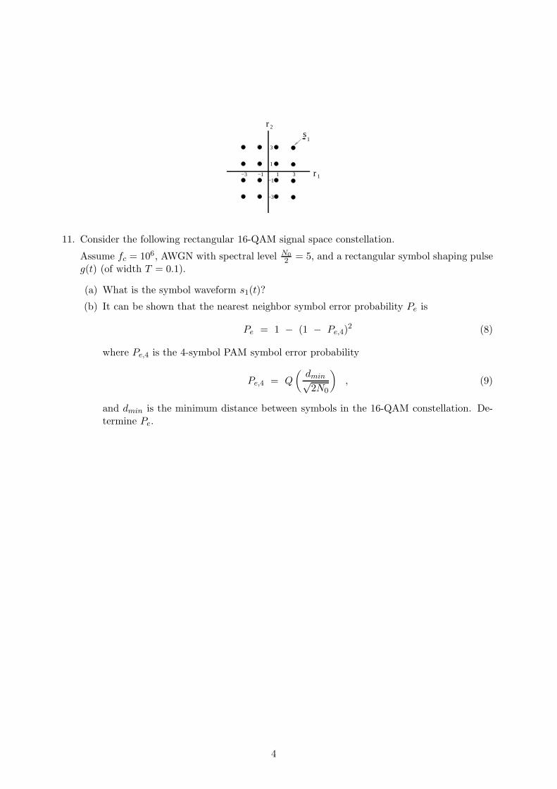
11. Consider the following rectangular 16-QAM signal space constellation.
Assume fc = 106, AWGN with spectral level N0
2= 5, and a rectangular symbol shaping pulse
g(t) (of width T = 0.1).
(a) What is the symbol waveform s1(t)?
(b) It can be shown that the nearest neighbor symbol error probability Pe is
Pe = 1 − (1 − Pe,4)2 (8)
where Pe,4 is the 4-symbol PAM symbol error probability
Pe,4 = Q
(
dmin√2N0
)
, (9)
and dmin is the minimum distance between symbols in the 16-QAM constellation. De-termine Pe.
4

Kevin Buckley - 2011 -1
ECE8700Communication Systems Engineering
Villanova UniversityECE Department
Prof. Kevin M. Buckley
Lecture 1
sourceinformation
encodersource channel
encodercommunication
channel
compressedinformation bits
transmittedsignal
receivedsignal
ai
informationoutputdecoder
sourcechanneldecoder
receivedsignal
ai^
compressedinformation bits
estimated estimatedinformation
modulator
s (t) r (t)
information
demodulator
r (t)^ ^
j
j
x
x C
C k
k
estimated
codeword.bits
codewordbits
Kevin Buckley - 2011 0
Contents
1 Introduction to and Background for Digital Communications 11.1 Digital Communication System Block Diagram . . . . . . . . . . . . . . . . . 2
1.1.1 Channel Considerations & a Little System Theory . . . . . . . . . . . 41.2 Bandpass Signals and Systems . . . . . . . . . . . . . . . . . . . . . . . . . . 8
1.2.1 A Directed Review of the CTFT . . . . . . . . . . . . . . . . . . . . 91.2.2 Real-Valued Bandpass (Narrowband) Signals & Their Lowpass Equiv-
alents . . . . . . . . . . . . . . . . . . . . . . . . . . . . . . . . . . . 181.2.3 Real-Valued Linear Time-Invariant Bandpass Systems . . . . . . . . . 22
List of Figures
1 Digital Communication system block diagram. . . . . . . . . . . . . . . . . . 22 Digital communication channel with additive noise & channel distortion. . . 43 Equivalent discrete-time model of modulator/channel/demodulator. . . . . . 64 The FIR equivalent discrete-time model (the z−1 block represent a sample
delay). . . . . . . . . . . . . . . . . . . . . . . . . . . . . . . . . . . . . . . . 65 CTFT of a modulated sinc2 signal. . . . . . . . . . . . . . . . . . . . . . . . 146 Illustration of the multiplication property of the CTFT. . . . . . . . . . . . . 157 A CT LTI system and the convolution integral. . . . . . . . . . . . . . . . . 168 A CT LTI system and the frequency response. . . . . . . . . . . . . . . . . . 169 The spectrum of a bandpass real-valued signal. . . . . . . . . . . . . . . . . . 1810 The spectrum of the complex analytic signal corresponding to the bandpass
real-valued signal illustrated in Figure 9. . . . . . . . . . . . . . . . . . . . . 1911 The spectrum of the complex lowpass signal corresponding to the bandpass
real-valued signal illustrated in Figure 9. . . . . . . . . . . . . . . . . . . . . 1912 A receiver (complex demodulator) that generates the the complex lowpass
equivalent signal xl(t) from the original real-valued bandpass signal x(t). . . 2013 Energy spectra for: (a) the real-valued bandpass signal x(t); (b) its complex
lowpass equivalent xl(t). . . . . . . . . . . . . . . . . . . . . . . . . . . . . . 2114 Real-valued linear bandpass system. . . . . . . . . . . . . . . . . . . . . . . . 2215 Bandpass and equivalent lowpass systems and signals. . . . . . . . . . . . . . 23

Kevin Buckley - 2011 1
1 Introduction to and Background for Digital Commu-
nications
Over the past 60 years digital communication has had a substantial and growing influenceon society. With the recent worldwide growth of cellular and satellite telephone, and withthe Internet and multimedia applications, digital communication now has a daily impact onour lives and plays a central role in the global economy. Digital communication has becomeboth a driving force and a principal product of a global society.
Digital communication is a broad, practical, highly technical, deeply theoretical, dynam-ically changing engineering discipline. These characteristics make digital communication avery challenging and interesting topic of study. Command of this topic is necessarily a longterm challenge, and any course in digital communication must provide some tradeoff betweenoverview and more in-depth treatment of selective topics.
That said, the aim of this Course is to provide an introduction to basic topics in digitalcommunications. Specifically, we will:
• describe some of the more important digital modulation schemes;
• introduce maximum likelihood detection of modulation symbols and maximum likeli-hood estimation of symbol sequences, and evaluate their performance for various digitalmodulation schemes;
• become familiar with the Viterbi algorithm as well as other efficient algorithms forsequence estimation;
• consider the need and methods for implementing carrier and symbol synchronization;
• consider bandlimited channels and intersymbol interference, and introduce optimumchannel equalization for mitigating these; and
• briefly overview adaptive equalization, multicarrier and spread spectrum communica-tions, fading channels and MIMO systems, and multiuser communications.
For these objectives we will need to first establish some background in signal & systemdescriptions, probability, and linear algebra. Before we proceed with this, let’s consider thebasic components of a digital communication system.

Kevin Buckley - 2011 2
1.1 Digital Communication System Block Diagram
Figure 1 is a block diagram of a typical digital communication system. This figure is followedby a description of each block, and by accompanying comments on their relationship to thisCourse.
sourceinformation
encodersource channel
encodercommunication
channel
compressedinformation bits
transmittedsignal
receivedsignal
ai
informationoutputdecoder
sourcechanneldecoder
receivedsignal
ai^
compressedinformation bits
estimated estimatedinformation
modulator
s (t) r (t)
information
demodulator
r (t)^ ^
j
j
x
x C
C k
k
estimated
codeword.bits
codewordbits
Figure 1: Digital Communication system block diagram.
The information source and information output represent the both subject of the com-munication and the locations, respectively, of transmission and reception. They representthe application. Examples of subjects include: voice, music, images, video, text, and variousforms of data. Examples of transmission/reception pairs include: phone to phone, cell-phoneto base-station, terminal to terminal, sensor to processor, and ground-station to satellite.This Course is a general introduction to digital communication, so we will not focus on anyspecific application.
The source encoder transforms signals to be transmitted into information bits, Xj , whileimplementing data compression for efficient representation for transmission. Source codingtechniques include: fixed length codes (lossless); variable length Huffman codes (lossless);Lempel Ziv coding (lossless); sampling & quantization (lossy); adaptive differential pulsecode modulation (ADPCM) (lossy); and transform coding (lossy). Although source codingis not covered in this Course, it is a principal topic of ece8247 Multimedia Systems and asecondary topic of ece8771 Information Theory and Coding for Digital Communications.
The channel encoder introduces redundancy into the information bits to form the codewordsor code sequences, Ck, so as to accommodate receiver error management. Channel codingapproaches included: block coding; convolutional coding, turbo coding, space-time coding

Kevin Buckley - 2011 3
and coded modulation. Although channel encoding is not covered in this Course, it is aprincipal topic of ece8771 Information Theory and Coding for Digital Communications.
The digital modulator transforms information or codeword bits into waveforms (symbols)which can be transmitted over a communication channel. A M-ary digital modulationscheme, characterized by its M symbols (for transmission of binary information, M is typ-ically a power of two), governs this transformation. Digital modulation schemes include:Pulse Amplitude Modulation (PAM); Frequency Shift Keying (FSK); M-ary QuadratureAmplitude Modulation (M-QAM); and Binary Phase Shift Keying (BPSK) & QuadraturePhase Shift Keying (QPSK). The description, receiver processing and performance of digitalmodulation schemes is a primary topic of this Course.
The communication channel is at the heart of the communication problem. Additive chan-nel noise corrupts the transmitted digital communication signal, causing unavoidable symboldecoding errors at the receiver. The channel also distorts the transmitted signal, as charac-terized by the channel impulse response. We further discuss these forms of signal corruptionin Subsection 1.1.1 below. Additionally, at the channel output interfering signals are oftensuperimposed on the transmitted signal along with the noise. In this Course we are primarilyinterested in the control of errors caused by both additive noise and channel distortion.
The digital demodulator is the signal processor that transforms the distorted, noisy receivedsymbol waveforms into discrete time data from which binary orM-ary symbols are estimated.Demodulator components include: correlators or matched filters (which include the receiverfront end); nearest neighbor threshold detectors; channel equalizers; symbol detectors andsequence estimators. Design of the digital demodulator is a principal topic of this Course.We also consider channel equalizers and sequence estimators which used to compensate ofchannel distortion of the transmitted symbols. These are rich and challenging topics. Anin-depth treatment of these topics is beyond the scope of this Course – they are principaltopics of ece8770 Topics in Digital Communications.
The channel decoder works in conjunction with the channel encoder to manage digital com-munication errors. Although channel encoding is not covered in this Course, it is a principaltopic of ece8771 Information Theory and Coding for Digital Communications.
The source decoder is the receiver component that reverses, as much as possible or reason-able, the source coder. Although source coding is not covered in this Course, it is a principaltopic of ece8247 Multimedia Systems and a secondary topic of ece8771 Information Theoryand Coding for Digital Communications.
In summary, in this Course we are interested in the three blocks in Figure 1 from node(a) to node (b).
Kevin Buckley - 2011 4
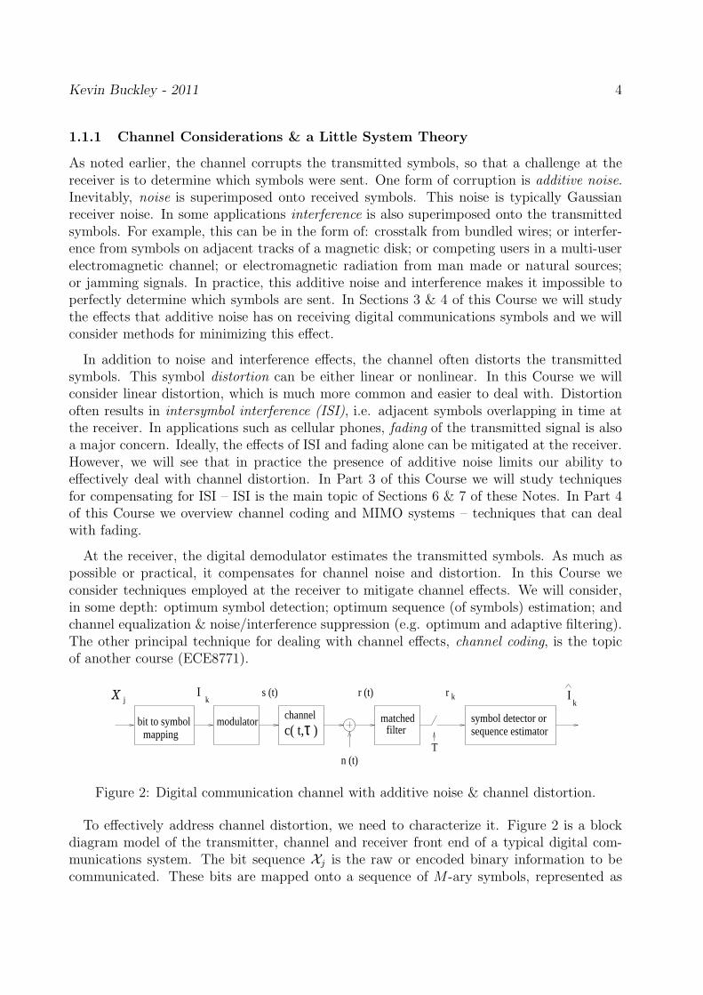
1.1.1 Channel Considerations & a Little System Theory
As noted earlier, the channel corrupts the transmitted symbols, so that a challenge at thereceiver is to determine which symbols were sent. One form of corruption is additive noise.Inevitably, noise is superimposed onto received symbols. This noise is typically Gaussianreceiver noise. In some applications interference is also superimposed onto the transmittedsymbols. For example, this can be in the form of: crosstalk from bundled wires; or interfer-ence from symbols on adjacent tracks of a magnetic disk; or competing users in a multi-userelectromagnetic channel; or electromagnetic radiation from man made or natural sources;or jamming signals. In practice, this additive noise and interference makes it impossible toperfectly determine which symbols are sent. In Sections 3 & 4 of this Course we will studythe effects that additive noise has on receiving digital communications symbols and we willconsider methods for minimizing this effect.
In addition to noise and interference effects, the channel often distorts the transmittedsymbols. This symbol distortion can be either linear or nonlinear. In this Course we willconsider linear distortion, which is much more common and easier to deal with. Distortionoften results in intersymbol interference (ISI), i.e. adjacent symbols overlapping in time atthe receiver. In applications such as cellular phones, fading of the transmitted signal is alsoa major concern. Ideally, the effects of ISI and fading alone can be mitigated at the receiver.However, we will see that in practice the presence of additive noise limits our ability toeffectively deal with channel distortion. In Part 3 of this Course we will study techniquesfor compensating for ISI – ISI is the main topic of Sections 6 & 7 of these Notes. In Part 4of this Course we overview channel coding and MIMO systems – techniques that can dealwith fading.
At the receiver, the digital demodulator estimates the transmitted symbols. As much aspossible or practical, it compensates for channel noise and distortion. In this Course weconsider techniques employed at the receiver to mitigate channel effects. We will consider,in some depth: optimum symbol detection; optimum sequence (of symbols) estimation; andchannel equalization & noise/interference suppression (e.g. optimum and adaptive filtering).The other principal technique for dealing with channel effects, channel coding, is the topicof another course (ECE8771).
X
modulatorc( t, )τchannel
kr
filtermatched
kI
bit to symbolmapping
s (t)
n (t)
kI r (t)
j
T
symbol detector orsequence estimator
Figure 2: Digital communication channel with additive noise & channel distortion.
To effectively address channel distortion, we need to characterize it. Figure 2 is a blockdiagram model of the transmitter, channel and receiver front end of a typical digital com-munications system. The bit sequence Xj is the raw or encoded binary information to becommunicated. These bits are mapped onto a sequence of M-ary symbols, represented as

Kevin Buckley - 2011 5
the Ik. The Ik modulate a carrier sinusoid to form the signal s(t), e.g.
s(t) =∑
k
Ik g(t− kT ) , (1)
which is transmitted across the channel. Here g(t) is the analog symbol pulse shape and Tis the symbol duration (i.e. the inverse of the symbol rate).
The channel shown in Figure 2 is assumed to be linear and time-varying with time-varyingimpulse response c(t, τ). To better understand what this channel impulse response c(t, τ)signifies, first consider a Linear Time-Invariant (LTI) channel. Let c(t) represent its impulseresponse, which means that if the impulse δ(t) is applied to the channel input (at time t = 0),the channel output (i.e. its response) will be c(t). Note that since the input δ(t) has energythat is completely concentrated at time t = 0, and since the corresponding output c(t) isspread over time, the channel has memory (e.g. due to multipath propagation). Since weare assuming that the channel is time-invariant, the channel response to the delayed impulseδ(t − τ) will be the delayed impulse response c(t − τ). Since the channel is assumed tobe linear, and since any signal s(t) can be expressed as a linear combination of of delayedimpulses (i.e. s(t) =
∫
s(τ) δ(t− τ) dτ), the channel output will be
r(t) =∫
s(τ) c(t− τ) dτ + n(t) . (2)
This shows that the LTI channel output component due to the signal s(t) is a convolutionof s(t) with the channel impulse response c(t), i.e. s(t) ∗ c(t). In this equation, t denotes“output time” or current time, whereas τ represents “memory time” (i.e. the output at“output time” t is a function of the input in general over all time, via the integration overall “memory time” τ).
Now let the channel be linear but time-varying. Denote as c(t, τ) the output due to inputδ(t− τ). That is, if we apply an impulse to the channel input at time τ , the channel outputwill be c(t, τ), which is a function of time t which depends on the time τ when the impulsewas applied. Now, since the channel is again assumed to be linear, and since any signal s(t)can be expressed as s(t) =
∫
s(τ) δ(t− τ) dτ , the channel output will be
r(t) =∫
s(τ) c(t, τ) dτ + n(t) . (3)
The receiver problem which we focus on in this Course is to process the received signal r(t)so as to determine the transmitted symbols Ik.
In this Course we will take the traditional approach to dealing linear time-varying chan-nels. That is, we will develop receiver methods for LTI channels and then, for time-varyingchannels, develop adaptive implementations which can track channel variation over time.

Kevin Buckley - 2011 6
Typically, the front end of a digital communication receiver consists of a demodulator anda matched filter. In Figure 2 this front end is referred to simply as the matched filter. We willconsider the receiver front end in Section 3.1 of this Course. Its output is a Discrete-Time(DT) sequence which we denote as rk. The rate of this sequence is the same as the symbolrate fs (i.e.
1T, the rate of the Ik). The rk sequence is a distorted, noisy version of the desired
symbol sequence Ik. The symbol detector or sequence estimator will process the rk to forman estimated sequence Ik of the symbol sequence Ik.
Figure 3 depicts an equivalent discrete-time model, from Ik to rk, of the digital communi-cation system shown in Figure 2.
kr
channel modeldiscrete−timeequivalent
+
kn
kI
Figure 3: Equivalent discrete-time model of modulator/channel/demodulator.
In Part 2 of this Course we will consider a simple special case of this model, for which thenoise nk is Additive White Gaussian Noise (AWGN) and the channel is distortionless (i.e. ithas no effect). For this case,
rk = Ik + nk . (4)
In Part 3 we will characterize and address channel distortion. For this case, we will refinethe general model shown in Figure 3, specifically showing that the channel can be modeledas a Finite Impulse Response (FIR) filter. For the time-invariant channel case, this this filterhas fixed coefficients as shown in Figure 4.
f 0 f 1 f L
z−1 z−1 z−1I n
vn
η n
present inputsymbol
.....
I In−1 n−L
past input symbols
Figure 4: The FIR equivalent discrete-time model (the z−1 block represent a sample delay).
L is the memory depth of the channel (i.e. the number of past symbols that distort theobservation of the current symbol), and the fl; l = 0, 1, · · · , L are the FIR filter modelcoefficients which reflect how the channel linearly combines the present and past symbols.

Kevin Buckley - 2011 7
The matched filter output sequence is then
rk =L∑
l=0
fl Ik−l + nk . (5)
The impulse response for this FIR filter model is
fk = f0 δk + f1 δk−1 + · · · + fL δk−L , (6)
where δk is the DT impulse function. This equivalent discrete-time model, shown on p. 627of the Course Text, is very useful since it is a broadly applicable and relatively easy to workwith. In lectures, homework problems, and computer assignments we will use the followingthree examples of a equivalent discrete-time channel (given in terms of their impulse responserepresentations):
1. Bandlimited (e.g. wireline) channel (from text, p. 654): f0 = f2 = 0.407;f1 = 0.815; fk = 0 otherwise.
2. From text (p. 687): fk = 0.8δ(k)− 0.6δ(k − 1).
3. Magnetic tape recording channel: f0 = f13 = 0.004184;f1 = f12 = 0.009072; f2 = f11 = 0.012473; f3 = f10 = 0.030223;f4 = f9 = 0.058746; f5 = f8 = 0.172583; f6 = f7 = 0.18659;fk = 0 otherwise.
For the linear time-varying channel case, the equivalent DT model I/0 equation will be ofthe form
rk =L∑
l=0
fk,l Ik−l + nk . (7)

Kevin Buckley - 2011 8
1.2 Bandpass Signals and Systems
This Section of the Course corresponds to Section 2.1 of the Course Text. We introducenotation and basic signals & systems concepts which are needed to describe digital modula-tion schemes. This discussion assumes some familiarity with signals & systems theory andin particular the Continuous-Time Fourier Transform (CTFT). We begin with a directedreview of the CTFT.
Typically, the frequency components (in Hertz) of a transmitted communication signalhave much higher frequencies than the bandwidth of the transmitted signal. We term sucha signal a bandpass signal. It has frequency components which are restricted to a band offrequencies which is small compared to the frequencies of the signal. Typically, an informa-tion signal that we are interested in is a baseband signal. It has frequency components whichare restricted to a small band of frequencies around DC (zero Hertz). Transmitted bandpasssignals are generated from a baseband information signal, by the transmitter, through aprocess called modulation. At the receiver, this signal is often translated back to the orig-inal (baseband) frequency range. For this and other reasons it is convenient to represent atransmitted signal, as well as the channel that carry it, in terms of its equivalent lowpass(a.k.a. baseband) representation.
The objective of this Section is to develop an equivalent lowpass representation of a mod-ulated (bandpass) communication signal, as well as the lowpass representation of the system(i.e. of the modulator, channel & demodulator) associated with it. This representation isbroadly applicable for both baseband and bandpass communication systems. The advantageof this representation, which we will use throughout the Course, is that we can use it todescribe, analyze and design communication systems. In particular, we can represent sig-nals processing components of interest in this Course without having to concern ourselveswith specific frequency ranges and modulation. This equivalent lowpass representation alsofacilitates comparison between different modulation schemes.
The frequency content of a Continuous-Time (CT) signal is determined and represented asthe CT Fourier Transform (CTFT) of that signal. We begin this discussion with a directedreview of the CTFT.

Kevin Buckley - 2011 9
1.2.1 A Directed Review of the CTFT
The Continuous-Time Fourier Transform (CTFT, Fourier transform for short) is usuallyexpressed in terms of angular frequency ω (in radians/second) as
X(ω) =∫ ∞
−∞x(t) e−jωt dt , (8)
and the corresponding inverse CTFT
x(t) =1
2π
∫ ∞
−∞X(ω) ejωt dω . (9)
Eq (9) indicates that x(t) can be represented as or decomposed into a linear combinationof all the CT complex-valued sinusoids ejωt over the frequency range −∞ ≤ ω ≤ ∞. Thisequation, called the Inverse CTFT (ICTFT), is the synthesis equation since it generates x(t)from basic sinusoidal signals. Eq (9) is called the analysis equation because it derives theweighting function X(jω) for the synthesis equation1. Often the notation X(jω) = X(ω) isused which shows the relationship between the Fourier transform and the Laplace transform,i.e. X(jω) = X(s) |s=jω where X(s) is the Laplace transform of x(t). Table 1.1 provides alist of some commonly encountered CTFT pairs.
Sometimes, for example in the Course Text, the CTFT is described in terms of frequencyf = ω
2π(inHz. = cycles/second). To do this, take the Fourier transform integral equations
above and substitute f = ω2π, resulting in the equivalent transform pair
X(f) =∫ ∞
−∞x(t) e−j2πft dt , (10)
x(t) =∫ ∞
−∞X(f) ej2πft df . (11)
Table 2.0-2, on p. 19 of the Course Text, provides Fourier transform pairs in terms offrequency (in Hertz). To be consistent with the Course Text, we will use the less commonEqs (10,11) notation.
1Proof of the CTFT involves plugging Eq (8) into Eq (9) and simplifying to show that the right side ofEq (9) does reduce to x(t). This simplification, specifically a change of the order of two nested integrals,requires certain assumptions. These assumptions are that x(t): be absolutely integrable, and have a finitenumber of minima/maxima and discontinuities. The absolutely integrable requirement essentially (but notexactly) means that x(t) be an energy signal. Therefore, strictly speaking, the CTFT is not applicable toperiodic signals such as sinusoids since periodic signals are power signals. However, the CTFT is commonlyemployed to represent periodic signals by using an impulse in X(jω) to represent each harmonic component.

Kevin Buckley - 2011 10
Table 1.1: Continuous Time Fourier Transform (CTFT) Pairs.
# Signal CTFT(∀ t) (∀ ω)
1 δ(t) 1
2 δ(t− τ) e−jωτ
3 u(t) 1jω
+ πδ(ω)
4 e−atu(t); Rea > 0 1a+jω
5 te−atu(t); Rea > 0 1(a+jω)2
6 tn−1
(n−1)!e−atu(t); Rea > 0 1
(a+jω)n
7 e−a|t|; Rea > 0 2aa2+ω2
8 pT (t) = u(t+ T2)− u(t− T
2) 2
ωsin
(
ωT2
)
9 1πtsin(Wt) p2W (ω)
10 sin2(Wt)(πt)2
12π
p2W (ω) ∗ p2W (ω)
11 cc2+t2
π e−c|ω|
12 ejω0t 2πδ(ω − ω0)
13 cos(ω0t) πδ(ω − ω0) + πδ(ω + ω0)
14 sin(ω0t)πjδ(ω − ω0)−
πjδ(ω + ω0)
15 ak ejkω0t 2πak δ(ω − kω0)
16∞∑
k=−∞
ak ejkω0t∞∑
k=−∞
2πak δ(ω − kω0)
17∞∑
n=−∞
δ(t− nT ) 2πT
∞∑
k=−∞
δ(
ω −2π
Tk)

Kevin Buckley - 2011 11
Example 2.1: Consider the signal x(t) = δ(t − t0). Determine its CTFT X(f).Based on the result, comment on the frequency content of the signal.
Solution:
Note the consistence between the time and frequency domain representationsof this signal. x(t) changes infinitely over zero time, which implies very highfrequency components. In fact, X(f) indicates that the impulse consists of equalcontent over all frequency. It’s the most wideband signal. This Example derivesEntries #1 & #3 of Table 2.0-2 of the Course Text.
Example 2.2: Determine the CTFT, X(f), of the signal x(t) = p2T1(t) (i.e. a
pulse, centered at t = 0, of width 2T1; using the notation established on p. 17of the Course Text, p2T1
(t) = Π( t2T1
)). Based on the result, comment on thefrequency content of the signal.
Solution:
Note that X(f) has infinite extent, indicating that it contains infinitely high fre-quency components. This should not be surprising since x(t) has discontinuities,which require infinitely high frequency components to synthesize. Also note theX(f) is largest for lower frequencies, indicating that in some sense x(t) in mostlya low frequency signal. This Example derives Entry #7 of Table 2.0-2 of theCourse Text.
Kevin Buckley - 2011 12
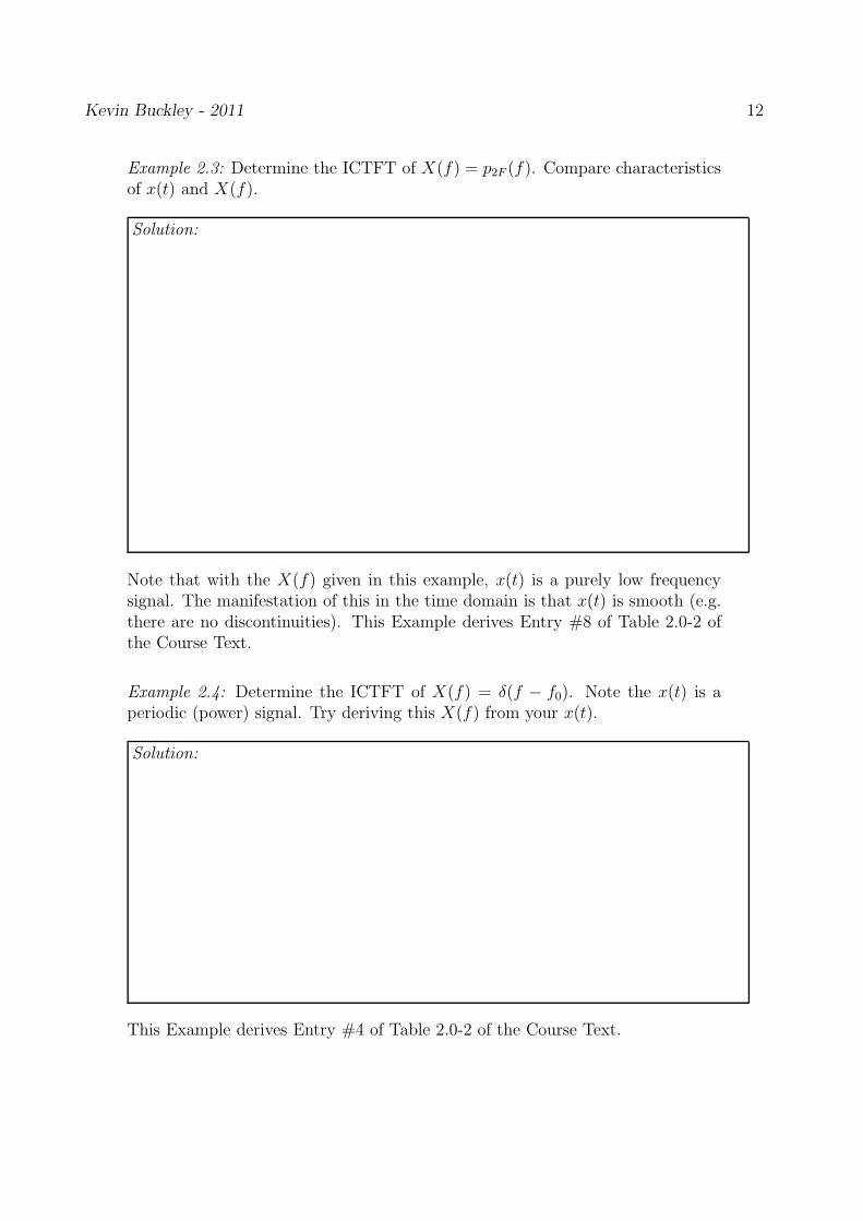
Example 2.3: Determine the ICTFT of X(f) = p2F (f). Compare characteristicsof x(t) and X(f).
Solution:
Note that with the X(f) given in this example, x(t) is a purely low frequencysignal. The manifestation of this in the time domain is that x(t) is smooth (e.g.there are no discontinuities). This Example derives Entry #8 of Table 2.0-2 ofthe Course Text.
Example 2.4: Determine the ICTFT of X(f) = δ(f − f0). Note the x(t) is aperiodic (power) signal. Try deriving this X(f) from your x(t).
Solution:
This Example derives Entry #4 of Table 2.0-2 of the Course Text.

Kevin Buckley - 2011 13
Table 2.0-1, p. 18 of the Course Text, lists some of the more useful properties of theCTFT. Of particular interest in this Course are:
1. Symmetry – for real-valued x(t), X(f) is complex-symmetric, i.e. X(−f) = X∗(f).
2. Linearity –α x1(t) + β x2(t) ←→ α X1(f) + β X2(f) , (12)
e.g. the CTFT of a superposition of a signal and noise is the superposition of theCTFTs of the signal and the noise.
3. Modulation –ej2πfot x(t) ←→ X(f − f0) . (13)
That is, multiplication by a complex sinusoid ej2πfot shifts the frequency content by f0.Combining the modulation and linearity properties with Euler’s identities, we have
cos(2πfot) x(t) ←→1
2[X(f − f0) + X(f + f0)] (14)
sin(2πfot) x(t) ←→1
2j[X(f − f0) − X(f + f0)] . (15)
4. Convolution –x(t) ∗ h(t) ←→ X(f) H(f) . (16)
H(f), the CTFT of the impulse response, is called the frequency response. Since, fora CT LTI channel with impulse response c(t), the output y(t) due to input s(t) isy(t) = s(t) ∗ c(t), the output frequency content is given by Y (f) = S(f) C(f).
5. Parseval’s Theorem – the energy of a CT signal x(t) (e.g. a communication symbol) is
Ex =∫ ∞
−∞|x(t)|2 dt =
∫ ∞
−∞|X(f)|2 df . (17)
In Table 2.0-1 of the Course Text, this property is referred to as the Rayleigh Theorem.
6. Multiplication –
x(t) · y(t) ←→ X(f) ∗ Y (f) =∫ ∞
−∞X(λ) Y (f − λ) dλ . (18)
Example 2.5: Let x(t) = 2πt
sin(100πt). Determine the % of energy over thefrequency band −25 ≤ f ≤ 25.
Solution:

Kevin Buckley - 2011 14
Example 2.6: Plot the magnitude and phase spectra of x(t) = δ(t− 5).
Solution:
Example 2.7: Determine the CTFT of x(t) = 2 sin2(πF t)π2Ft2
cos(2πf0t), wheref0 > F .
Solution: Start with entry #10 of Table 2.0-2 of the Course Text and the time-scale property of the CTFT given in Table 2.0-1. Then, using the modulationproperty of the CTFT, we have the result shown in the figure below.
CTFT
CTFT2
2
sin ( Ft)π
π F t2
2
2
sin ( Ft)π
π F t2cos (2 f t)π
0
1
F−Ff
2f
f f−f −f0 0+F 0 0+F
1
Figure 5: CTFT of a modulated sinc2 signal.

Kevin Buckley - 2011 15
Example 2.8: Let x(t) have CTFT as illustrated below. Its important feature,for this example, is that its frequency content is bandlimited to −W ≤ ω ≤ W .Determine the CTFT of
xT (t) = x(t) · p(t) ; p(t) =∞∑
n=−∞
δ(t− nT )
Assume that T < πW.
Solution:
p(t)
t0 T 2T 3T−T
(1)......
π(2 /T)
ω
ω
t
x(t)
0
......
−ω ω 3ω2ω ω0 0 0 0
A
T
A/T
t0 2T−T
......
x (t)T
3T
(x(0))
T(x(T))
W−W
W
0
......
−ω ω 3ω2ω ω0 0 0 0
P( )
X ( )ω
ω
X( )
Figure 6: Illustration of the multiplication property of the CTFT.
In Example 2.8, note that since T < πW
is assumed, we have that ω0
2> W , and there is no
overlap in Xp(ω) of the shifted images of X(ω). Since the impulse rate is fs =1T, we can say
that the impulse rate is fast enough, relative to the highest frequency W of x(t), to avoidoverlapping of the shifted images of X(ω). This has very important consequences related tothe sampling and reconstructions of CT signals.
Kevin Buckley - 2011 16
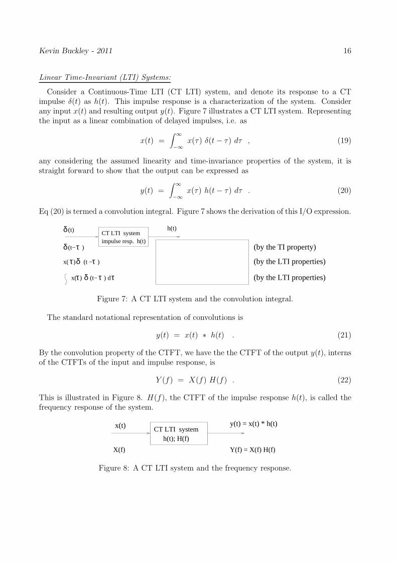
Linear Time-Invariant (LTI) Systems:
Consider a Continuous-Time LTI (CT LTI) system, and denote its response to a CTimpulse δ(t) as h(t). This impulse response is a characterization of the system. Considerany input x(t) and resulting output y(t). Figure 7 illustrates a CT LTI system. Representingthe input as a linear combination of delayed impulses, i.e. as
x(t) =∫ ∞
−∞x(τ) δ(t− τ) dτ , (19)
any considering the assumed linearity and time-invariance properties of the system, it isstraight forward to show that the output can be expressed as
y(t) =∫ ∞
−∞x(τ) h(t− τ) dτ . (20)
Eq (20) is termed a convolution integral. Figure 7 shows the derivation of this I/O expression.
(by the TI property)
(by the LTI properties)
(by the LTI properties)
δ
δ
δ
δ
(t) h(t)
(t− )τimpulse resp. h(t)CT LTI system
x( ) (t− ) dτ
τ
ττ
x( ) (t − )τ
Figure 7: A CT LTI system and the convolution integral.
The standard notational representation of convolutions is
y(t) = x(t) ∗ h(t) . (21)
By the convolution property of the CTFT, we have the the CTFT of the output y(t), internsof the CTFTs of the input and impulse response, is
Y (f) = X(f) H(f) . (22)
This is illustrated in Figure 8. H(f), the CTFT of the impulse response h(t), is called thefrequency response of the system.
CT LTI systemx(t) y(t) = x(t) * h(t)
h(t); H(f)
Y(f) = X(f) H(f)X(f)
Figure 8: A CT LTI system and the frequency response.

Kevin Buckley - 2011 17
Example 2.9: Consider a CT LTI system with impulse response h(t) = sinc(2π100t).Determine the output due to:
a) x1(t) = sinc(2π50t); and
b) x2(t) = 3 cos(2π10t) = 5 cos(2π200t).
Solution:

Kevin Buckley - 2011 18
1.2.2 Real-Valued Bandpass (Narrowband) Signals & Their Lowpass Equiva-lents
This discussion corresponds to Subsection 2.1.1 of the Course Text.
Consider a real-valued bandpass, narrowband signal x(t) with center frequency fc andCTFT
X(f) =∫ ∞
−∞x(t) e−j2πft dt , (23)
where X(f), as illustrated below in Figure 9, is complex symmetric2. In the context of thisCourse, x(t) will be a transmitted digital communications symbol or signal (i.e. a modulatedsignal that is the input to a communication channel).
A
f−f fcc
X(f)
Figure 9: The spectrum of a bandpass real-valued signal.
Let u−1(f) be the step function (i.e. u−1(f) = 0; f < 0; u−1(f) = 1; f > 0). The analyticsignal for x(t) is defined as follows:
X+(f) = u−1(f) X(f) (24)
andx+(t) =
∫ ∞
−∞X+(f) e
j2πft df . (25)
By the CTFT convolution property,
x+(t) = x(t) ∗ F−1u−1(f) , (26)
where F−1u−1(f) is the inverse CTFT of u−1(f). X+(f) is sketched in Figure 10 for theX(f) illustrated previously.
Note that, from the CTFT pair table, the inverse CTFT of the frequency domain stepu−1(f) used above is
g(t) =1
2δ(t) +
j
2h(t) , h(t) =
1
πt(27)
where δ(t) is the impulse function. It can be shown that h(t) is a 90o phase shifter, andx(t) = x(t) ∗ h(t) is termed the Hilbert transform of x(t). So, by the convolution propertyof the CTFT,
x+(t) = x(t) ∗ g(t) =1
2x(t) +
j
2x(t) ∗ h(t) =
1
2x(t) +
j
2x(t) (28)
2For illustration purposes, X(f) is shown as real-valued. In general, it is complex-valued. Since x(t) isassumed real-valued, the magnitude of X(f) is even symmetric. It’s phase would be odd symmetric.

Kevin Buckley - 2011 19
f−f fcc
X (f)+
A
Figure 10: The spectrum of the complex analytic signal corresponding to the bandpassreal-valued signal illustrated in Figure 9.
where x(t) and x(t) are real-valued. Also, from the definition of x+(t) and CTFT properties,note that
x(t) = x+(t) + x∗+(t) = 2Rex+(t) . (29)
The equivalent lowpass of x(t) (also termed the complex envelope) is, by definition,
Xl(f) = 2 X+(f + fc) , (30)
xl(t) = 2 x+(t) e−j2πfct (31)
where fc is the center frequency of the real-valued bandpass signal x(t). We term this signalthe lowpass equivalent because, as illustrated in Figure 11 for the example sketched outpreviously, xl(t) is lowpass and it preserves sufficient information to reconstruct x(t) (i.e. itis the positive, translated frequency content). Note that
x+(t) =1
2xl(t) e
j2πfct . (32)
So,x(t) = Rexl(t) e
j2πfct , (33)
and also
X(f) =1
2[Xl(f − fc) +X∗
l (−f − fc)] . (34)
Then, given xl(t) (say it was designed), x(t) is easily identified (as is xl(t) from x(t)).
f−f fc
2A
c
X (f)l
Figure 11: The spectrum of the complex lowpass signal corresponding to the bandpass real-valued signal illustrated in Figure 9.

Kevin Buckley - 2011 20
Figure 12 shows several approaches for generating the lowpass equivalent xl(t) from anoriginal bandpass signal x(t). Figure 12(a), based on Eqs (28,31), illustrates how to generatethe lowpass equivalent using a Hilbert transform (as notes earlier, h(t) = 1
πtis the impulse
response of the Hilbert transform). From Figure 12(a), we have that
xl(t) = 2 x+(t) e−j2πfct = 2 (x(t) + jx(t))
1
2(cos(2πfct) − j sin(2πfct)) (35)
= (x(t) cos(2πfct) + x(t) sin(2πfct)) + j (x(t) cos(2πfct) − x(t) sin(2πfct)) .(36)
This implementation is shown in Figure 12(b). Figure 12(c) shows an equivalent circuitbased on a quadrature receiver. Here, x(t) is complex modulated to baseband and lowpassfiltered so as to translate its positive frequency content to baseband and capture only that.The frequency response of the lowpass filter would be
H(f) =
2 −fm ≤ f ≤ fm0 otherwise
, (37)
where fm is the one-sided bandwidth of the desired signal. The filtered output xi(t) of thecosine demodulator is termed the in-phase component, and the filtered output xq(t) of thesine demodulator is termed the quadrature component. Combined, as shown, they form thecomplex-valued quadrature receiver output which is xl(t).
h(t) j
+
+
x(t)
x(t)
x (t)+
h(t)
cos(2 f t)π c
H(f)
H(f)
x (t)q
x (t)i
x (t)i
x (t)q
x (t)lx(t)demodulator
x(t)
(d)
(b)
e π−j2 f tc
(a)
(c)
x(t)^
π c
π c
sin (2 f t)
sin (2 f t)
+
+
+
+
x(t)
cπcos(2 f t)
π−sin(2 f t)c
x (t) = x (t) + j x (t)i ql
π ccos(2 f t)
lx (t)2
Figure 12: A receiver (complex demodulator) that generates the the complex lowpass equiv-alent signal xl(t) from the original real-valued bandpass signal x(t).
Relating all of this to the communications problem, since the received signal in a commu-nications system is typically a real-valued bandpass signal (e.g. x(t) in the above discussion)and since the then typically receiver demodulates this signal down to baseband (e.g. xl(t) isthe above discussion), Figures 12(a-c) show three equivalent receiver demodulators. Figure12(d) represents either of these three in block diagram form.

Kevin Buckley - 2011 21
To summarize our development of a lowpass equivalent communication signal to this point,starting with a real-valued bandpass signal x(t), we have
x(t) = 2 Rex+(t) = Rexl(t) ej2πfct , (38)
where the analytic signal x+(t) and the lowpass equivalent xl(t) can be generated from x(t)as illustrated in Figure 12. The in-phase and quadrature components, xi(t) and xq(t), canbe used together to generate the lowpass equivalent from the original x(t).
Since xl(t) = xi(t) + j xq(t) is complex-valued, it can be expressed in terms of itsmagnitude and phase, i.e.
xl(t) = rx(t) ejθx(t) ; rx(t) =
√
x2i (t) + x2
q(t) ; θx(t) = tan−1
(
xq(t)
xi(t)
)
. (39)
Then xi(t) = rx(t) cos(θx(t)) and xq(t) = rx(t) sin(θx(t)), and we have that
x(t) = Rerx(t) ej(2πfct+θx(t)) = rx(t) cos(2πfct + θx(t)) . (40)
rx(t) and θx(t) are, respectively, the envelope and phase of x(t).
The energy of x(t) is, by Parseval’s theorem,
Ex =∫ ∞
−∞|X(f)|2 df . (41)
Figure 13 demonstrates that Ex can be calculated from xl(t) as
Ex =1
2Exl
=1
2
∫ ∞
−∞|Xl(f)|
2 df . (42)
A2 4A2
(a) (b)
f−f fcc
2
f
2X(f) X (f)
l
Figure 13: Energy spectra for: (a) the real-valued bandpass signal x(t); (b) its complexlowpass equivalent xl(t).
Note the need for the 12factor. This is because the spectral levels of Xl(f) are twice that
of the positive frequency components of X(f) (a gain in amplitude of 2 corresponds to again in energy of 4), but the negative frequency components of x(t) (i.e. half the energy ofx(t)) are not present in Xl(f).

Kevin Buckley - 2011 22
1.2.3 Real-Valued Linear Time-Invariant Bandpass Systems
This discussion corresponds to Subsection 2.1-4 of the Course Text.
Let the narrowband bandpass real-valued signal x(t) considered above be the input to aLinear, Time-Invariant (LTI) bandpass system as illustrated below in Figure 14. Within thecontext of this Course, this system is a cascade of the communications channel, the trans-mitter & receiver filters, and the front end antenna electronics. With a lowpass equivalentmodel, the transmitter/receiver modulators (i.e. the frequency shifters) are also represented.
−fc fc
H(f)
f
h(t), H(f)x(t) y(t)
X(f) Y(f)
Figure 14: Real-valued linear bandpass system.
Let h(t) and H(f) denote the LTI system impulse and frequency responses, related as aCTFT pair. From linear system theory, and the convolution property of the CTFT, theoutput is
y(t) = x(t) ∗ h(t) (43)
with CTFTY (f) = X(f)H(f) . (44)
We wish to determine an equivalent lowpass representation for the system and the outputthat can be used in conjunction with the lowpass equivalent, of the input, xl(t). Withthese, we will be able to couch the communication problems of interest in terms of a lowpassequivalent system representation.
Consider a equivalent lowpass representation of h(t) which parallels that which we havealready developed for x(t), i.e.
h(t) = Rehl(t) ej2πfct . (45)
Thus, we have that
H(f) =1
2[Hl(f − fc) + H∗
l (−f − fc)] . (46)
Then the output Fourier transform, in terms of lowpass equivalents is
Y (f) = X(f) H(f) =1
4[Xl(f − fc) +X∗
l (−f − fc)] [Hl(f − fc) +H∗l (−f − fc)]
=1
4Xl(f − fc)Hl(f − fc) +X∗
l (−f − fc)H∗l (−f − fc)
+ Xl(f − fc)H∗l (f − fc) +X∗
l (−f − fc)Hl(f − fc) . (47)

Kevin Buckley - 2011 23
Under the assumption that x(t) is passband and narrowband (i.e. fc is large compared tothe bandwidth), and that h(t) is passband covering only the frequencies of x(t), the last twoterms in the above equation are zero, and so
Y (f) =1
4[Xl(f − fc)Hl(f − fc) +X∗
l (−f − fc)H∗l (−f − fc)] . (48)
If we also define y(t) in terms of yl(t) as
y(t) = Reyl(t) ej2πfct , (49)
Y (f) =1
2[Yl(f − fc) + Y ∗
l (−f − fc)] , (50)
Then the relationship between Yl(f) and Xl(f) & Hl(f) must be
Yl(f) =1
2Xl(f) Hl(f) , (51)
yl(t) =1
2xl(t) ∗ hl(t) . (52)
Note the factor of 12in both the time and frequency domain lowpass equivalent input/output
relationships.Figures 15 (a),(b) and (c) show, respectively, a bandpass system, the conversion (demod-
ulation) to baseband, and the equivalent lowpass system. Signal energy levels are indicated.
quadraturereceiver h (t)
l
1
2
(a) (c)(b)
h(t)εε 2ε 2ε
y(t)
x y
y (t)y(t) x (t)
x y
y (t) = x (t) * h (t)x(t)l llll
Figure 15: Bandpass and equivalent lowpass systems and signals.
Kevin Buckley - 2011 22
ECE8700Communication Systems Engineering
Villanova UniversityECE Department
Prof. Kevin M. Buckley
Lectures 2-3
s
s s
s
s2
s1
s2
s1
2
3 4
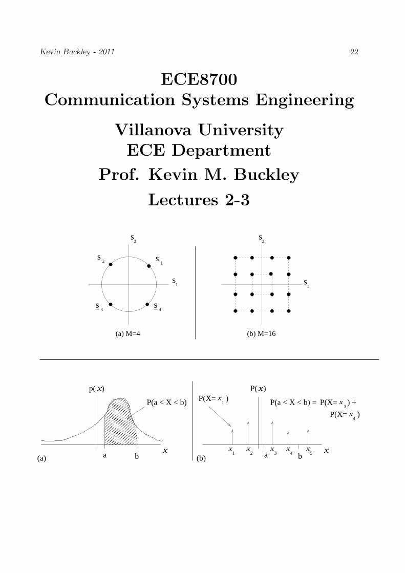
1
(a) M=4 (b) M=16
p( )x
P(a < X < b)
x
ba
x1
P(X= )x
3P(X= ) +
xP(X= )4
P(a < X < b) =
x1
x x x x
(a) (b)
x
x2 3 4 5
P( )
a b

Kevin Buckley - 2011 23
Contents
1 Introduction to and Background for Digital Communications 241.1 Digital Communication System Block Diagram . . . . . . . . . . . . . . . . . 241.2 Bandpass Signals and Systems . . . . . . . . . . . . . . . . . . . . . . . . . . 241.3 Representation of Digital Communication Signals . . . . . . . . . . . . . . . 24
1.3.1 Vector Space Concepts . . . . . . . . . . . . . . . . . . . . . . . . . . 241.3.2 Vector Spaces for Continuous-Time Signals . . . . . . . . . . . . . . . 271.3.3 Signal Space Representation & Euclidean Distance Between Waveforms 281.3.4 Symbol Sequence Representation & the DTFT . . . . . . . . . . . . . 31
1.4 Selected Review of Probability and Random Processes . . . . . . . . . . . . 341.4.1 Probability . . . . . . . . . . . . . . . . . . . . . . . . . . . . . . . . 341.4.2 Random Variables . . . . . . . . . . . . . . . . . . . . . . . . . . . . 371.4.3 Statistical Independence and the Markov Property . . . . . . . . . . 411.4.4 The Expectation Operator & Moments . . . . . . . . . . . . . . . . . 421.4.5 Gaussian Random Variables . . . . . . . . . . . . . . . . . . . . . . . 481.4.6 Other Random Variable Types of Interest . . . . . . . . . . . . . . . 501.4.7 Bounds on Tail Probabilities . . . . . . . . . . . . . . . . . . . . . . . 521.4.8 Weighted Sums of Multiple Random Variables . . . . . . . . . . . . . 541.4.9 Random Processes . . . . . . . . . . . . . . . . . . . . . . . . . . . . 55
List of Figures
16 Examples of N = 2 dimensional signal space diagrams. . . . . . . . . . . . . 2817 A N = 2 dimensional signal space diagram (for a digital communication
modulation scheme) showing geometric features of interest. . . . . . . . . . . 3018 Illustration of the use of orthonormal functions as receiver filter bank impulse
responses. . . . . . . . . . . . . . . . . . . . . . . . . . . . . . . . . . . . . . 3019 An illustration of the union bound. . . . . . . . . . . . . . . . . . . . . . . . 3620 A PDF of a single random variable X , and the probability P (a < X < b):
(a) continuous-valued; (b) discrete-valued. . . . . . . . . . . . . . . . . 3721 (a) A tail probability; (b) a two-sided tail probability for the Chebyshev in-
equality. . . . . . . . . . . . . . . . . . . . . . . . . . . . . . . . . . . . . . . 5222 g(Y ) function for (a) the Chebyshev bound, (b) the Chernov bound. . . . . . 5323 Power spectral densities of: (a) the original bandpass process; and (b) the
lowpass equivalent process. . . . . . . . . . . . . . . . . . . . . . . . . . . . . 6824 Power spectrum density of bandlimited white noise. . . . . . . . . . . . . . . 68
Kevin Buckley - 2011 24
1 Introduction to and Background for Digital Commu-
nications
1.1 Digital Communication System Block Diagram
1.2 Bandpass Signals and Systems
1.3 Representation of Digital Communication Signals
This Subsection of the Course Notes corresponds to Section 2.2 of the Course Text.
The objective here is to develop a generally applicable framework for studying digitallymodulated communication symbols and corresponding received signals. In this Subsectionwe will introduce this framework, termed the signal space representation, and in Section 2 ofthis Course we will apply it to represent several common digital communication modulationschemes. This signal space representation of digital communication symbols will be basedon:
• a basis expansion of the set of symbols employed in the modulation scheme; and
• a Euclidean measure of the distance between symbols (i.e. a geometric representation).
Later, when we discuss the channel and demodulator, we will combine this signal spacerepresentation of a modulation scheme with the equivalent lowpass representation of a digitalcommunication system.
Below, we first briefly overview the representation of vectors in a vector space. We thenshow how continuous-time signals (e.g. digital communication symbols) can be representedin terms of these vectors and we describe how this leads to a the signal space representationof digital communication symbols. We end this Subsection with a discussion of symbolsequences, including a directed review of the Discrete-Time Fourier Transform (DTFT).
1.3.1 Vector Space Concepts
It is tempting to begin this discussion with a basic and formal treatment of algebra, introduc-ing the concept of a set of elements, then a group, then elementary arithmetic (i.e. additionand multiplication operators), then a field, then multiplication, and then finally a vectorspace and an inner product. Such a discussion would provide the framework necessary tostudy coding theory, which is an advanced digital communications topic. However, for thisintroductory consideration of digital communications, this formality is not necessary. So wewill keep this discussion somewhat informal.
In general, a vector space is defined over a set of elements which could be, for example,continuous-time signals, discrete-time signals, polynomials, or row or column vectors. In thisCourse, since we are interested in conveniently representing digital communications symbolswhich are transmitted over a channel, we will mainly be interested in continuous-time signals.However, to develop the concepts we require to understand the standard representation ofcommunication symbol, i.e. the signal space representation, we will begin with a review ofvector spaces for column vectors, since this is what engineers are typically most familiarwith.

Kevin Buckley - 2011 25
Consider an n-dimensional complex-valued column vector vk:
vk = [vk,1, vk,2, ...vk,n]T , (1)
where the superscript “T” denotes transpose. We say that vk is a vector in the n-dimensionalcomplex vector space, which we denote as Cn. (If vk is real-valued, we say it is in the realvector space Rn.) The inner product of two such vectors vk and vj is defined as
< vk, vj > = vHj vk =n∑
i=1
vk,i v∗j,i , (2)
where the superscript “H” denotes complex conjugate transpose (a.k.a. Hermitian trans-pose). Two vectors, vk and vj, are said to be orthogonal if
< vk, vj > = 0. (3)
The Euclidean norm (a.k.a. norm, L2 norm) of a vector vk is defined as
||vk|| =(
vHk vk) 1
2 , (4)
A vector vk has unit norm if ||vk|| = 1.Consider a set of m n-dimensional vectors, vk; k = 1, 2, · · · , m, and scalars sk; k =
1, 2, · · · , m. The following is a linear combination (a.k.a. weighted sum) of the vectors:
v =m∑
k=1
sk vk = V s (5)
where V = [v1, v2, ..., vm] is an (n × m)-dimensional matrix and s = [s1, s2, ..., sm]T is an
m-dimensional column vector. The set of all possible linear combinations of the vk; k =1, 2, · · · , m is called the span of the vk; k = 1, 2, · · · , m. The span of these vectors is asubspace of vector space Cn.
Given a set of m ≤ n vectors v1, v2, · · · , vm, we say that the set is linearly independentif no one vector in the set can be written as linear combination of the m − 1 others. (Notethat m > n n-dimensional vectors can not be linearly independent.) A basis for a subspaceof Cn is a set, of minimum number, of vectors in the subspace which can be used to representany vector in the subspace as a linear combination. The vectors forming a basis must belinearly independent. Let p denote this minimum number of vectors. Then the dimensionof the subspace is defined as p. Clearly, 0 ≤ p ≤ n. If p = 0 we say the subspace in the nullspace. If p = n, the subspace is Cn itself. One reason that a basis is important is the we candefine a p-dimensional subspace as the set of all linear combinations (i.e. the span) of its pbasis vectors, and we can represent any vector in the subspace as a linear combination of itsbasis vectors.
Let v1, v2, · · · , vm be a set of vectors and let V = [v1, v2, · · · , vm] be the (n × m)-dimensional matrix whose columns are these vectors. The rank of these vectors is defined asthe dimension p of their span. So the rank is the number of vectors in the basis. For m ≤ n,if p = m, we say that the vectors v1, v2, · · · , vm, or equivalently the matrix V , is full-rank.

Kevin Buckley - 2011 26
Let v1, v2, · · · , vm, m ≤ n, form a basis for an m-dimensional subspace. This basis iscalled an orthogonal basis if
< vk, vj > = 0 ; ∀ i 6= j . (6)
Additionally, if< vk, vk > = 1 ; k = 1, 2, · · · , m , (7)
i.e. if all basis vectors have unit norm, we say the the basis is orthonormal.Orthonormal bases facilitate a simple representation of vectors. For example, let v1, v2, · · · , vn
be an orthonormal basis for Cn. Then any n-dimensional complex vector v can be expanded(and represented) as
v =n∑
k=1
sk vk = V s (8)
where V = [v1, v2, ..., vn], s = [s1, s2, ..., sn]T , and sk = vHk v. That is, any v can be written
as a linear combination of the orthonormal basis vectors, where the coefficients of the linearcombination are obtained simply as inner products.
Consider an arbitrary n-dimensional vector v, a set ofm < n orthonormal vectors v1, v2, · · · , vm,and the matrix V = [v1, v2, · · · , vm]. In general, v can not be represented as a linear combina-tion of these m orthonormal vectors. Even so, consider the rank-m (low-rank) approximationof v:
v =m∑
k=1
sk vk = V s (9)
with, as before, sk = vHk v. The error vector for this low-rank approximate representation is
e = v − v = v − V s . (10)
Ee = ||e||2 is the energy of the error. It can be shown that the s used above, (s = V Hv),minimizes the error energy. It can also be shown that
Ee = ||v||2 − ||s||2 =n∑
i=1
|vi|2 −m∑
i=1
|si|2 . (11)
This discussion on basic vector space concepts and terminology provides background fordescribing a signal space representation of digital communication symbols. It also developsan understanding which is generally very useful for signal processing and communications.In the end, for this Course, we minimally need to be comfortable with the signal space rep-resentation. Nonetheless, you should strive to be comfortable with these basic concepts, asrepresented by the following terms: inner product, orthogonal, norm, Euclidean norm, unitnorm, linear combination, weighted sum, span, subspace, linear independent, basis, dimen-sion, null space, rank, orthogonal basis, orthonormal basis, and low-rank.

Kevin Buckley - 2011 27
1.3.2 Vector Spaces for Continuous-Time Signals
Consider a complex-valued continuous-time signal x(t) over range of time [a, b]. In thisCourse this range will usually be either all time [−∞,∞] or a digital communication symbolinterval such as [0, T ] for symbol duration T . For this type of signal we define the innerproduct as
< x1(t), x2(t) > =∫ b
ax1(t) x
∗2(t) dt (12)
and the Euclidean norm as
||x(t)|| = < x(t), x(t) >1/2 =
(
∫ b
a|x(t)|2 dt
)1/2
. (13)
Consider a set of N orthonormal signals (functions) φi(t); i = 1, 2, · · · , N. Then bydefinition
< φi(t), φj(t) > = δ[i− j] . (14)
These functions from and orthonormal basis for their N -dimensional span (i.e. as withvectors, the span is the set of all linear combinations).
Let s(t) be a signal, and φk(t); k = 1, 2, · · · , K a set of K orthonormal functions. Con-sider the low-rank approximation
s(t) =K∑
k=1
sk φk(t) . (15)
Define the approximation error as e(t) = s(t)− s(t). The energy of the error is
Ee = ||e(t)||2 =∫ b
a|e(t)|2 dt . (16)
It can be shown that this error energy is minimized using expansion coefficients
sk = < s(t), φk(t) > k = 1, 2, · · · , K . (17)
The resulting minimum error energy is
Ee = ||s(t)||2 − ||s(t)||2 = ||s(t)||2 − ||s||2 ; s = [s1, s2, · · · , sK ]T (18)
or Ee = Es − Es.

Kevin Buckley - 2011 28
1.3.3 Signal Space Representation & Euclidean Distance Between Waveforms
Let sm(t); m = 1, 2, · · · ,M be M waveforms (corresponding to communication symbolswithin the context of this Course). For this general discussion we will consider them overthe range of time [−∞,∞]. Consider orthonormal expansion of these waveforms in terms ofthe N ≤ M orthonormal functions φk(t); k = 1, 2, ..., N which form a basis for the sm(t)
′s.(These waveforms and corresponding basis functions could be either real-valued bandpass orcomplex-valued lowpass equivalents. Here will use complex notation.) The expansion is
sm(t) =N∑
k=1
smk φk(t) = φ(t) sm (19)
where smk = < sm(t), φk(t) >, sm = [sm1, sm2, · · · , smN ]T , and
φ(t) = [φ1(t), φ2(t), · · · , φN(t)].
A signal space diagram is a plot, in N -dimensional space, of the sm vectors. sm is thesignal space representations of the waveforms sm(t). Figure 16 shows two examples of N = 2dimensional signal space diagrams.
s
s s
s
s2
s1
s2
s1
2
3 4
1
(a) M=4 (b) M=16
Figure 16: Examples of N = 2 dimensional signal space diagrams.
The Euclidean distance between sm(t) and sk(t) is defined as
d(e)km =
(∫ ∞
−∞|sm(t)− sk(t)|2 dt
) 1
2
. (20)
Noting that∫∞−∞ φH(t)φ(t) dt = IN (the N -dimensional identity matrix), we have
d(e)km =
(∫ ∞
−∞|φ(t) sm − φ(t) sk|2 dt
) 1
2
(21)
=(
sHm sm + sHk sk − sHk sm − sHm sk) 1
2 (22)
= ||sm − sk|| . (23)
This is a key result. It states that the Euclidean distance between two waveforms is equalto the Euclidean distance between the coefficient vectors of their orthonormal expansions.This provides a geometric interpretation of distances between waveforms.

Kevin Buckley - 2011 29
Using Eq (22) we can rewrite this Euclidean distance as
d(e)km =
(
Em + Ek − 2ResHm sk) 1
2 , (24)
or
d(e)km =
(
Em + Ek − 2√
EmEk ρmk
) 1
2
(25)
where
ρmk = cos θmk =ResHmsk||sm|| ||sk||
, (26)
termed the correlation coefficient for sm(t) and sk(t), is the cosine of the angle θmk betweenthe two signal space representations sm and sk. For example, for two equal energy waveforms(i.e. Em = Ek = E),
d(e)km = (2E(1− cos θmk))
1
2 (27)
which is maximized for θmk = 180o (i.e sm and sk colinear but of opposite sign).As we will see, efficient digital communications occurs when Euclidean distances between
digital transmission symbols (which are waveforms) are maximized. Typically, for multiplesymbol digital modulation schemes, bit-error-rate is dominated by the minimum of the Eu-clidean distances between all of the symbols. Since, for a modulation scheme, the Euclideandistances between symbol waveforms in important, and since these distances can be easilyidentified in terms of their orthonormal expansion coefficient vectors (that is, in terms oftheir signal space representation), it is this representation that is commonly used to describemany modulation schemes.
Figure 17 shows the signal space diagram of M = 12 waveforms in an N = 2 dimensionalsignal space. An angle between two signals, and the minimum Euclidean distance betweenany two signals, dmin, are shown. The signal space diagram of the symbols of a digitalcommunication modulation scheme is often referred to as the constellation of the modulationscheme.

Kevin Buckley - 2011 30
mind
s2
s1
s1
s2
1,2θ
Figure 17: A N = 2 dimensional signal space diagram (for a digital communication modu-lation scheme) showing geometric features of interest.
In conjunction with the signal space representations of the symbols of a modulationscheme, we will use orthonormal expansions of received signals to describe optimum re-ceivers for processing the continuous time channel output r(t). Figure 18 illustrates theidea. A bank of N filters, whose impulses responses are the N orthogonal basis functions ofthe symbols of the employed modulation scheme, form the receiver preprocessor. We will seethat these filters represent the receiver front end (i.e. the front end demodulator and filters).We will also see that these filters form the inner products between the received signal and thebases functions for modulation scheme. Thus for the given modulation scheme these filtersderive the signal space representation vector rn, at symbol time n, of the received signalr(t). Subsequently, this vector rn will be compared to the modulation scheme constellationto “detect” the transmitted symbol. We will use this idea both to: 1) show that the outputof the bank of basis function filters can be processed as effectively as processing r(t) directly,by comparing rn to the modulation scheme constellation; and 2) to show that samples ofthe basis function filter outputs form a sufficient statistic of r(t) (i.e. processing only thesamples, we can achieve performance equivalent to processing the whole continuous timesignal). When showing these points later on, we can use either the received signal directlyor its equivalent lowpass representation.
φ
φ
r(t) = s(t)+n(t) ....
nT
Detection
or
SequenceEstimation
r
1 (t)
(t)K
n
Figure 18: Illustration of the use of orthonormal functions as receiver filter bank impulseresponses.

Kevin Buckley - 2011 31
1.3.4 Symbol Sequence Representation & the DTFT
In Subsection 1.1.1 of these Course Notes, within a discussion of the digital communicationchannel, we introduced a Discrete-Time (DT) channel model. The input to this channelmodel is the digital communication symbol sequence, which we denote as Ik (as a functionof symbol index k). At the time, we did not indicate what specifically the Ik would look like.We will see in Section 2 of these Course Notes that for several of the most important digitalmodulation schemes, Ik will be a sequence of real-valued or complex-valued numbers derivedfrom the signal space representation of the modulation scheme. So we will be interested inworking with DT sequences.
Recall that earlier we modeled a LTI digital communication channel as a DT FIR filterwith impulse response fk. So we will be working with DT systems.
The Discrete-Time Fourier Transform (DTFT) and the z-transform are two transformsthat are commonly used to analyze and design DT signals and systems. In this Coursewe will use the DTFT in Lectures 3 & 4 to characterize the frequency content of digitalcommunications signals. Later, in Part 3 of this Course, we will briefly use the DTFT andthe z-transform to develop the the DT FIR filter model fk of a LTI digital communicationchannel. Here we briefly describe the DTFT in only enough detail to meet our future needs.We will introduce the z-transform in Part 3 of this Course.
The DTFT of a DT signal xn is
X(ej2πf) =∞∑
n=−∞
xn e−j2πfn (28)
where the Inverse DTFT (the IDTFT) is
xn =∫ 1/2
−1/2X(ej2πfn) ej2πfn df (29)
Eq (29) is called the synthesis equation because it shows how a signal xn can be representedas a linear combination of the complex sinusoids ej2πfn; −1
2< f ≤ 1
2. Eq (28) is called
the analysis equation because it computes the weighting function X(ej2πf) applied to theej2πfn in Eq (29) (i.e. it evaluates xn to determine its frequency content). The units of fare cycles/sample and ω = 2πf is in radians/sample. Being an orthonormal expansion of ageneral signal in terms of complex sinusoids (i.e. Eq (29)), it is very similar to the CTFTconsidered earlier. For example, properties are very similar, and our uses the CTFT andDTFT are very similar. Compared to the CTFT, the main difference with the DTFT is thatsince the signal x[n] is DT, we only use frequency over the range −1
2< f ≤ 1
2. This is because
of the ambiguity of DT sinusoidal frequency outside this range (i.e. ej2π(f+k)n = ej2πfn forand f and integer k). Table 1.2 provides some useful DTFT pairs. Table 1.3 lists someDTFT properties.

Kevin Buckley - 2011 32
Table 1.2: Discrete Time Fourier Transform (DTFT) Pairs
Signal DTFT1
(∀n) (−12≤ f ≤ 1
2)
1 δ[n− k] e−j2πfk
2 1π
1(1+n2)
e−|2πf |
3 anu[n]; |a| < 1 11−ae−j2πf
4 (n+ 1)anu[n]; |a| < 1 1(1−ae−j2πf )2
5 (n+r−1)!n!(r−1)!
anu[n]; |a| < 1 1(1−ae−j2πf )r
6 pN [n] = u[n]− u[n−N ] e−j2πf N−1
2
sin(N2πf
2 )sin( 2πf
2 )
7 u[n+N1]− u[n− (N1 + 1)]sin(2πf(N1+
1
2))
sin( 2πf
2 )
8 sin(Wn)πn
; 0 < W ≤ π
1 0 ≤ |2πf | ≤ W0 W < |2πf | ≤ π
9 δ[n] − 2sin2(π
2n)
(πn)2
2πf 0 ≤ 2πf ≤ π−2πf −π ≤ 2πf ≤ 0
10 a|n| 1−a2
(1+a2)−2a cos 2πf
11 an cos(2πf0n) u[n]1 − [a cos(2πf0)] e−j2πf
1 − [2a cos(2πf0)] e−j2πf + a2e−j4πf
12 an sin(2πf0n) u[n][a sin(2πf0)] e−j2πf
1 − [2a cos(2πf0)] e−j2πf + a2e−j4πf
13 ej2πf0n ; −π ≤ 2πf0 ≤ π δ(f − f0)
14N−1∑
k=0
ak ej(2π/N)nkN−1∑
k=0
ak δ(
f − 2π
Nk)
; 0 ≤ 2πf < 2π

Kevin Buckley - 2011 33
Table 1.3: Discrete Time Fourier Transform (DTFT) Properties.
Property Time Domain Frequency Domain
Periodicity x[n] X(ej2πf) = X(ej(2πf+2π)); ∀f
Symmetry real-valued x[n] X(−ej2πf) = X∗(ej2πf)
Delay x[n− k] X(ej2πf) e−j2πfk = |X(ej2πf)| ej[ 6 X(ej2πf )−2πfk]
Linearity a1x1[n] + a2x2[n] a1 X1(ej2πf) + a2 X2(e
j2πf)
Convolution x[n] ∗ h[n] X(ej2πf) H(ej2πf)
Parseval’s Theorem E =∞∑
n=−∞
|x[n]|2 E =∫
−1/2
1/2
|X(ej2πf)|2df
Modulation x[n] ej2πf0n X(ej2π(f−f0))

Kevin Buckley - 2011 34
1.4 Selected Review of Probability and Random Processes
Topics in this Section of the Course are from Chapter 2 of the Course Text. Here ourobjective is a review of probability and random process concepts which is directed towards thedigital communications problem – of digital demodulation of the output of a communicationschannel. Given a received communications signal,
r(t) = s(t) ∗ c(t) + n(t) , (30)
where s(t) is the modulated superimposed sequence of transmitted symbols representing thebinary or M-ary data, c(t) is the impulse response of the channel, and n(t) is the additivenoise and interference, we wish to accomplish one or more of the following:
• detect each symbol (i.e. at each symbol time n, decide which symbol was transmitted)– this requires a characterization of probability density functions (PDF’s) associatedwith the received signal r(t);
• estimation of the sequence of transmitted symbols, where the term “sequence estima-tion” is used to indicate the process of concurrent detection of a sequence of transmittedsymbols – joint PDF’s associated with the received signal r(t) will be required;
• optimally separate the signal s(t) from the noise and interference n(t) while accountingfor the effective of the channel impulse response c(t) – for the most part, at least inthis course, this will require 2-nd order statistical characterizations associated with thereceived signal r(t).
Here we informally cover just enough probability to get started. We will introduce morelater as we need it.
1.4.1 Probability
Consider what is called a random experiment, which is something that randomly generatesone from a number of possible outcomes. Typical introductory examples of such experimentsare a flip of a coin and a selection from a deck of cards. In engineering we are more interestedin in something like the voltage output of a sensor at some time.
We call an event some group of possible outcomes. The event of all possible outcomes iscalled the universal or certain event, which we denote as S here. The no outcome outcomeis the null event ∅. Let A and B denote any two events. Then, A∩B denotes the outcomesshared by A and B – the intersection of A and B. A ∪ B is the union of A and B. We saythat A and B are mutually exclusive if A ∩ B = ∅.
According to established rules probability, we assign probabilities to these events. LetP (A) denote the probability of event A. The three fundamental rules (axioms) from whichprobability is built are:
1. P (A) ≥ 0.
2. P (S) = 1.
3. If A and B are mutually exclusive, P (A ∩ B) = P (A) + P (B).

Kevin Buckley - 2011 35
From these three axioms of probability, all other probability rules can be derived. Forexample, in general
P (A ∪B) = P (A) + P (B) − P (A ∩ B) , (31)
and, for mutually exclusive A and B,
P (A ∩ B) = P (A) P (B) . (32)
Given a random event B and mutually exclusive, exhaustive (i.e. comprehensive) randomevents Ai; i = 1, 2, ..., n, with individual probabilities P (B) and P (Ai); i = 1, 2, ..., n,and joint probabilities P (Ai, B); i = 1, 2, ..., n, we have that
P (Ai, Aj) = 0 i 6= j (33)
because the Ai are mutually exclusive. We also have that
n∑
i=1
P (Ai) = 1 (34)
because the Ai are mutually exclusive and exhaustive. Also,
P (Ai/B) =P (Ai, B)
P (B)(35)
is the conditional probability equation. P (Ai/B) reads – the probability of event Ai givenevent B (has occurred). The relation
P (Ai/B) =P (B/Ai) P (Ai)
P (B)(36)
is Bayes’ theorem relating the conditional probabilities P (Ai/B) and P (B/Ai). The equation
P (B) =n∑
i=1
P (B/Ai) P (Ai) (37)
is the total probability (of B in terms of its conditional probabilities P (B/Ai)). Finally,
P (Ai/B) =P (B/Ai) P (Ai)
∑nj=1 P (B/Aj) P (Aj)
(38)
is Bayes’ theorem using the total probability for P (B).Within the context of this Course, we are often interested in the above relationships, where
Ai; i = 1, 2, · · · , n is the set of symbols used to representing binary data, and the event Bis related to received data. Since one and only one symbol is sent at a time, the symbol setis mutually exclusive and exhaustive. These notions can be extended from a single symbolto a sequence of transmitted symbols.

Kevin Buckley - 2011 36
Union Bound
As demonstrated in Chapter 4 of the Course Text and in Example 1.1 below, the unionbound on probability is useful in the performance analysis of digital modulation schemes.
Let Ei; i = 1, 2, · · ·N be events which are not necessarily mutually exclusive or exhaustive.We are often interested in the probability of the union of these events:
P
(
N⋃
i=1
Ei
)
. (39)
If the Ei were mutually exclusive, then
P
(
N⋃
i=1
Ei
)
=N∑
i=1
P (Ei) . (40)
This is illustrated in Figure 19(a) for the two event case. However, in general,
P
(
N⋃
i=1
Ei
)
≤N∑
i=1
P (Ei) , (41)
since if the events share some outcomes (elements), the probabilities are counted more thanonce with the summation over events on the right side of Eq (??). Figure 19(b) illustratesthis. The Eq (41) inequality is called the union bound. It upper bounds the probability thatat least one of the E ′
is will occur.
E1
E2
Venn Diagram
E1
E2
E1
E2
Venn Diagram
(b)(a)
Figure 19: An illustration of the union bound.
Example 1.1: Let Ii; i = 1, 2, · · · ,M represent theM possible symbols of a digitalmodulation scheme. Say symbol I1 was transmitted, and let Ii/I1; i = 2, 3, · · · ,Meach denote the event that a symbol Ii is decided over event I1 at the receiver.These M − 1 events are typically not mutual exclusive. P (Ii/I1), the probabilityof event Ii/I1, is usually easy to identify. Often, of interest is P (e/I1), theprobability of error given that I1 was transmitted. This is typically difficult toidentify. However, the union bound
P (e/I1) ≤M∑
i=2
P (Ii/I1) , (42)
is easy enough to identify, and often useful as a guideline for performance.

Kevin Buckley - 2011 37
1.4.2 Random Variables
A Single Random Variable
Let X be a random variable (RV) which takes on values x. The Probability DensityFunction (PDF) pX(x) and probability distribution function (a.k.a. cumulative distributionfunction) F (x1) are related as follows:
F (x) = P (−∞ < X ≤ x) =∫ x
−∞pX(u) du (43)
pX(x) =∂
∂xF (x) . (44)
The PDF has the following properties:
1. pX(−∞) = pX(∞) = 0.
2. pX(x) ≥ 0 ; ∀ x.
3.∫∞−∞ pX(x) dx = 1.
4. P (a < X ≤ b) =∫ ba pX(x) dx.
This last property is the reason that pX(x) is referred to as a probability density function -probabilities are computed by integrating over it (the area under the curve is the probability).A PDF is illustrated below2 in Figure 20 for both continuous and discrete-valued RVs.
p( )x
P(a < X < b)
x
ba
x1
P(X= )x
3P(X= ) +
xP(X= )4
P(a < X < b) =
x1
x x x x
(a) (b)
x
x2 3 4 5
P( )
a b
Figure 20: A PDF of a single random variable X , and the probability P (a < X < b):(a) continuous-valued; (b) discrete-valued.
2We will use a lower case p to denote a PDF of a continuous-valued RV, and an upper case P to representthe PDF of a discrete-valued RV.

Kevin Buckley - 2011 38
Example 1.2: Consider a continuous-valued random variable X with the followinguniform PDF
pX(x) =
1b−a
a < x ≤ b
0 otherwise(45)
with b > a.
x 1 x 2
b − a1
a b x (the values of X)
p (x)X
Let a < x1 < x2 < b. Determine an expression for P (x1 ≤ X < x2).
Solution:
P (x1 ≤ X ≤ x2) =x2 − x1
b − a
Example 1.3: Consider a discrete-valued random variable X with the followingPDF
PX(x) =N−1∑
k=0
Pk δ(x− xk) (46)
where the xk = k; k = 0, 1, · · · , N−1 are the discrete values the random variableX can take, and the Pk; k = 0, 1, · · · , N − 1 are the corresponding probabilities.In this Example, let Pk = 1
N. This is an example of a discrete-valued uniform
random variable.
Sketch this PDF. For N = 10, determine P (0 ≤ X ≤ 5).
Solution:
P (0 ≤ X ≤ 5) =∫ 5+
0−Px(x) dx =
5∑
k=0
Pk =5∑
k=0
1
10=
6
10.
The notation 0− and 5+ denotes, respectively, incrementally less that zero andincrementally greater than five.

Kevin Buckley - 2011 39
Multiple Random Variables
First consider two random variables X and Y . Their joint PDF is denoted pX,Y (x, y). Itis a 2-dimensional function of joint values of x and y.
Properties:
1. pX,Y (x, y) = 0 if either x or y are −∞ or ∞.
2. pX,Y (x, y) ≥ 0 ; ∀ x, y.
3.∫∞−∞
∫∞−∞ pX,Y (x, y) dy dx = 1.
4. P (a1 ≤ X < b1 and a2 ≤ X < b2) =∫ b1a1
∫ b2a2
pX,Y (x, y) dy dx.
As is the case for a single random variable, note that property 4. indicates why pX.Y (x, y) istermed a probability density - probabilities are computed by integrating over it. The volumeunder the pX,Y (x, y) surface is the probability.
Example 1.4: Consider random variables X = [X1, X2]T . Let
pX1,X2(x1, x2) =
8x1x2 0 ≤ x1 ≤ 1, 0 ≤ x2 ≤ x1
0 otherwise.
x 2
x 1
x 1
x 2
Region of Support
1
1
1
1
p (x , x )X ,X 1 2
1 2
The region-of-support is the range of values x for which the joint PDF is nonzero(i.e. the range of possible values of X).
Determine P (0.5 ≤ X1 ≤ 1, 0.5 ≤ X2 ≤ 1).
Solution:
P (0.5 ≤ X1 ≤ 1, 0.5 ≤ X2 ≤ 1) =∫ 1
.5
∫ x1
.5pX1,X2
(x1, x2) dx2 dx1 =∫ 1
.5
∫ x1
.58x1x2 dx2 dx1
= 8∫ 1
.5x1
(∫ x1
.5x2 dx2
)
dx1 = 8∫ 1
.5x1
(
x21
2− 1
8
)
dx1
= 8∫ 1
.5
(
x31
2− x1
8
)
dx1 = x41 −
x21
2
∣
∣
∣
∣
∣
1
.5
=9
16

Kevin Buckley - 2011 40
Given n RV’s, Xi; i = 1, 2, ..., n (in vector form X = [X1, X2, · · · , Xn]T ), their joint
PDF is denoted
pX1,X2,···,Xn(x1, x2, ..., xn) = pX(x) = p(x); x = [x1, x2, ..., xn]
T (47)
where the superscript ′′T ′′ denotes the matrix or vector transpose operation, and the “under-bar” indicates a vector or matrix (lower case represents a vector, while uppercase representsa matrix). The random variables can be either continuous (e.g. a sample of a received sig-nal), discrete (e.g. a communication symbol), or a combination of continuous and discrete.So, joint PDF’s can be either smooth (for continuous RV’s) or impulsive (for discrete RV’s)or combined smooth/impulsive (for a mix of continuous/discrete RV’s). We determine jointprobabilities of RV’s by integrating their joint PDF, i.e.
P (a < X ≤ b) =∫ b
ap(x) dx . (48)
Marginalization:
Consider X = [X1, X2, · · · , XN ]T partitioned, for example, as X1 = [X1, X2, · · · , XP ]
T
and X2 = [XP+1, XP+2, · · · , XN ]T . Select one of the partitions, say X1. We can determine
pX1(x1) from pX(x) by marginalizing (integrating) over X2 as follows:
pX1(x1) =
∫ ∞
−∞pX(x) dx2 . (49)
Conditional PDFs:
It follows from Bayes’ theorem that a conditional PDF of X1 given a value x2 of RV X2 is
p(x1/x2) =p(x1, x2)
p(x2)=
p(x2/x1) p(x1)
p(x2)(50)
where it is assumed that the value x2 is possible (i.e. p(x2) 6= 0). This last equation isparticularly useful for symbol detection and sequence estimation.
Note that if a RV X1 is discrete-valued (say a digital symbol) and X2 is continuous-valued(e.g. a sample of a received signal), we write
P (x1/x2) =p(x2/x1) P (x1)
p(x2). (51)
Again, this assumes that for the value of x2 considered, the PDF p(x2) is nonzero (i.e. thatvalue x2 can occur).

Kevin Buckley - 2011 41
1.4.3 Statistical Independence and the Markov Property
Note that in general a joint PDF of X does not factor into a product of the individual PDF’s,i.e. in general
p(x) 6=n∏
i=1
p(xi) . (52)
However, if it does for a particular X , then we say that these RV’s are statistically indepen-dent. In this case joint PDF will be a lot easier to work with (and the random vector X willbe easier to optimally process). If a set of random variables are statistically Independentand Identically Distributed, we refer to them as IID.
LetXj; j = 1, 2, · · · , n be a random sequence (a.k.a. random signal). LetX = [x1, x2, ..., xn]T .
We say this this sequence is a Markov process if joint PDF of X has the following factoriza-tion:
p(x) = p(x1) · p(x2/x1) · p(x3/x2) · · ·p(xn/xn−1) . (53)
You can imagine that Markov random process joint PDF’s are easier to work with thangeneral joint PDF’s, but not quite as easy to work with as statistically independent randomvariable PDF’s.
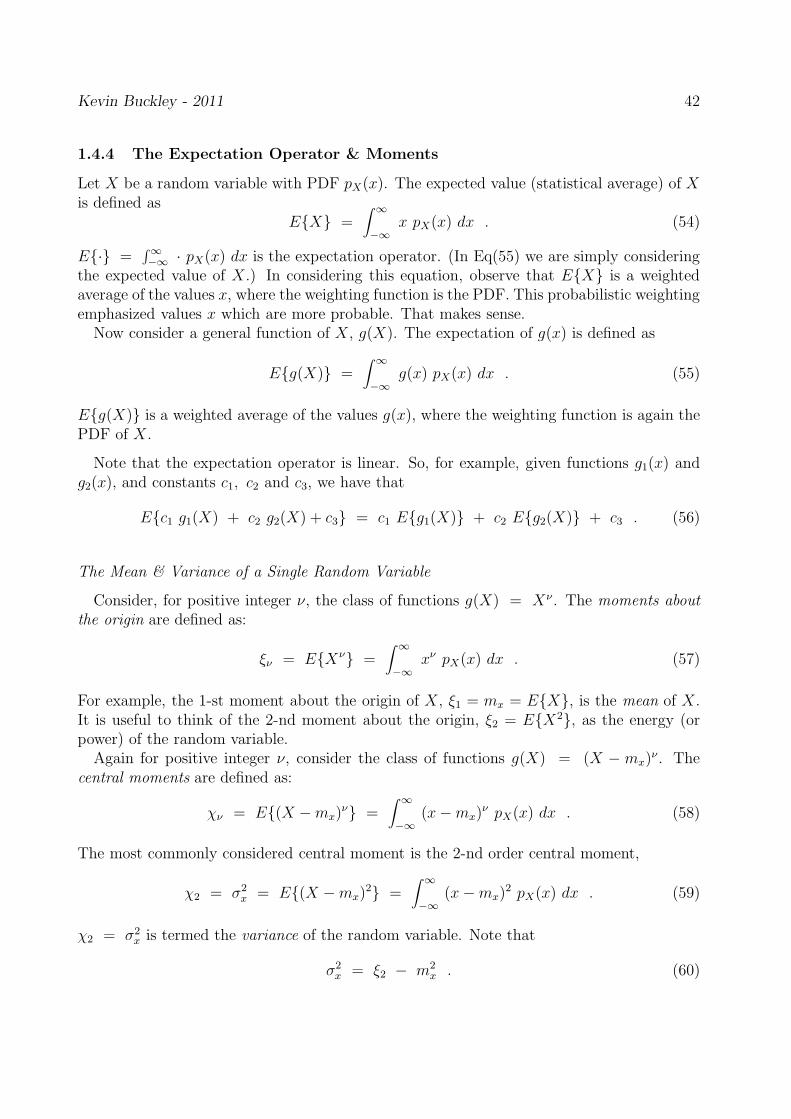
Kevin Buckley - 2011 42
1.4.4 The Expectation Operator & Moments
Let X be a random variable with PDF pX(x). The expected value (statistical average) of Xis defined as
EX =∫ ∞
−∞x pX(x) dx . (54)
E· =∫∞−∞ · pX(x) dx is the expectation operator. (In Eq(55) we are simply considering
the expected value of X .) In considering this equation, observe that EX is a weightedaverage of the values x, where the weighting function is the PDF. This probabilistic weightingemphasized values x which are more probable. That makes sense.
Now consider a general function of X , g(X). The expectation of g(x) is defined as
Eg(X) =∫ ∞
−∞g(x) pX(x) dx . (55)
Eg(X) is a weighted average of the values g(x), where the weighting function is again thePDF of X .
Note that the expectation operator is linear. So, for example, given functions g1(x) andg2(x), and constants c1, c2 and c3, we have that
Ec1 g1(X) + c2 g2(X) + c3 = c1 Eg1(X) + c2 Eg2(X) + c3 . (56)
The Mean & Variance of a Single Random Variable
Consider, for positive integer ν, the class of functions g(X) = Xν . The moments aboutthe origin are defined as:
ξν = EXν =∫ ∞
−∞xν pX(x) dx . (57)
For example, the 1-st moment about the origin of X , ξ1 = mx = EX, is the mean of X .It is useful to think of the 2-nd moment about the origin, ξ2 = EX2, as the energy (orpower) of the random variable.
Again for positive integer ν, consider the class of functions g(X) = (X − mx)ν . The
central moments are defined as:
χν = E(X −mx)ν =
∫ ∞
−∞(x−mx)
ν pX(x) dx . (58)
The most commonly considered central moment is the 2-nd order central moment,
χ2 = σ2x = E(X −mx)
2 =∫ ∞
−∞(x−mx)
2 pX(x) dx . (59)
χ2 = σ2x is termed the variance of the random variable. Note that
σ2x = ξ2 − m2
x . (60)

Kevin Buckley - 2011 43
Example 1.5: Determine the mean and variance of the uniform random variableX considered in Example 1.2.
Solution: For the mean,
mx =∫ b
a
1
b− ax dx =
1
b− a
x2
2
∣
∣
∣
∣
∣
b
a
=1
b− a
a2 − b2
2=
a+ b
2
For the variance, let q = b− a be the width of the density function. Then
σ2x =
1
q
∫ b
a
(
x− a + b
2
)2
dx =1
q
∫ q/2
−q/2x2 dx =
1
q
x3
3
∣
∣
∣
∣
∣
q/2
−q/2
=1
q
(
q3
24+
q3
24
)
=q2
12
The variance of a uniform random variable is σ2 = q2
12, i.e. the width squared
over twelve.
Example 1.6: Consider the linear transformation Y = g(X) = α X + β withpX(x) = u(x+ 1
2)− u(x− 1
2). Determine EY = Eα X + β.
Solution:
Eα X + β = Eα X+ Eβ = α EX+ β = β . (61)
Example 1.7: Determine the mean and variance of the exponential random vari-able X which has PDF
pX(x) = a e−ax u(x) . (62)
Assume a > 0.
Solution:

Kevin Buckley - 2011 44
Note that the mean of a random variable with symmetric PDF pX(x) is the point ofsymmetry.
Example 1.8: Determine the mean and variance of the random variable X whichhas PDF
pX(x) =1√2πc2
e−(x−c1)2/2c2 . (63)
Solution:
The Correlation and Covariance Between Two Random Variables
Consider two random variables X and Y , and let Z = g(X, Y ) be some function of them.The expectation of Z is
EZ = Eg(X, Y ) =∫ ∞
−∞
∫ ∞
−∞g(x, y) pX,Y (x, y) dx dy . (64)
This generalizes to g(Xi; i = 1, 2, · · · , N) is an obvious manner.Given two random variables X and Y , the ijth moment about the origin is
ξij = EX iY j =∫ ∞
−∞
∫ ∞
−∞xiyj pX,Y (x, y) dx dy . (65)
For example,
mX = ξ10 = EX1Y 0 = EX =∫ ∞
−∞
∫ ∞
−∞x pX,Y (x, y) dx dy
=∫ ∞
−∞x∫ ∞
−∞pX,Y (x, y) dy dx
=∫ ∞
−∞x pX(x) dx .

Kevin Buckley - 2011 45
Correlation, an important joint moment about the origin, is defined for random variablesX and Y as
φXY = ξ11 = EXY . (66)
We say that X and Y are uncorrelated if φXY = mX mY . We say that X and Y areorthogonal if φXY = 0.
Given two random variables X and Y , the ijth joint central moment is
χij = E(X−mX)i(Y −mY )
j =∫ ∞
−∞
∫ ∞
−∞(x−mX)
i(y−mY )j pX,Y (x, y) dx dy . (67)
For both joint central moments ξij and joint moments about the origin χij, the order of themoment is i+ j.
The covariance between X and Y , the 2-nd order central moment, is
σXY = χ11 = E(X −mX)(Y −mY ) . (68)
The correlation coefficient is defined as
ρXY =χ11√
χ20√χ02
=σXY
σX σY. (69)
Example 1.9: Consider two statistically independent random variables X and Y .Determine σXY and ρXY .
Solution:
Note that statistically independent random variables are uncorrelated (and orthogonalonly of mX = 0 and/or mY = 0). In general, uncorrelated does not necessarily implystatistically independent. Statistical independence say something about the entire jointPDF. Uncorrelated is only a 2-nd order characteristic.

Kevin Buckley - 2011 46
Example 1.10: Let P be a random variable with PDF
pP (p) =
12
−1 ≤ p < 10 otherwise
. (70)
Let Q = P 2 + 3. Determine EP, EP 2, EQ, φPQ, σPQ and ρPQ.
Solution:

Kevin Buckley - 2011 47
Moments of a Random Vector
Let X = [X1, X2, ..., Xn]T be a random vector. The mean of x, i.e. its expected value, is
EX =
EX1EX2
.
.
.EXn
= mx . (71)
The mean is termed the 1-st order moment. The correlation and covariance matrices of Xare, respectively,
Rx = EX XH =
φ1,1 φ1,2 · · · φ1,n
φ2,1 φ2,2 · · · φ2,n...
.... . .
...φn,1 φn,2 · · · φn,n
, (72)
and
Cx = E(X −mx)(X −mx)H =
σ1,1 σ1,2 · · · σ1,n
σ2,1 σ2,2 · · · σ2,n...
.... . .
...σn,1 σn,2 · · · σn,n
, (73)
where the superscript ′′H ′′ denotes Hermitian (complex conjugate) transpose. For example,the i, jth element of the covariance matrix Cx is
Cx[i, j] = σi,j = E(Xi − EXi)(Xj − EXj)∗ , (74)
where the superscript ′′∗′′ denotes conjugate.Note that Cx is Hermitian (complex conjugate) symmetric, i.e. CH
x = Cx, so
Cx[i, j] = C∗x[j, i] ∀ i, j . (75)
Note that Rx is also Hermitian. The covariance is termed the 2-nd order central moment(central because the mean is subtracted). Note that if
Cx[i, j] = 0 , (76)
the random variables Xi and Xj are uncorrelated. If Cx is diagonal, i.e. if
Cx = Diag σ21, σ2
2, · · · , σ2n (77)
where σ2i = σi,i = E|Xi|2, then the random variables in X are all mutually uncorrelated.
The eigenstructure of a covariance matrix Cx is important, for example, when studyingoptimum and adaptive equalizers. This eigenstructure is described as
Cx = V Λ V H , (78)
where V = [v1, v2, · · · , vn] is the n × n matrix whose columns are the orthonormal eigen-vector of Cx (note that V is therefore unitary), and Λ = Diagλ1, λ2, ..., λn is the diagonalmatrix of (real, non-negative) eigenvalues.

Kevin Buckley - 2011 48
1.4.5 Gaussian Random Variables
Consider a random variable X with PDF p(x). Its mean mx and variance σ2x are, respectively
mx = EX =∫ ∞
−∞x p(x) dx ; σ2
x = E|X−mx|2 =∫ ∞
−∞|x−mx|2 p(x) dx . (79)
A real-valued (as opposed to a complex-valued) Gaussian RV X has a PDF of the followingform:
p(x) =1
√
2πσ2x
e−(x−mx)2/2σ2x . (80)
A complex-valued random variable X = Xr + jXi is interpreted as a 2-dimensional variable(i.e. we can consider X = [Xr, Xi]
T ) and its PDF is actually the 2-dimensional joint PDFof [Xr, Xi]. A complex-valued RV is Gaussian if σ2
xr= σ2
xiand ρxrxi
= 0, so that its PDF is
p(x) =1
πσ2x
e−|x−mx|2/σ2x . (81)
where σ2x = σ2
xr+ σ2
xi.
Let X be an n-dimensional real-valued Gaussian random vector. Then, its joint PDF isof the form
p(x) =1
(2π)n/2(det(Cx))1/2
e−1
2(x−mx)
TC−1x (x−mx) (82)
where ′′ det “ denotes the determinant, mx = EX is the mean vector, and C−1x is the
matrix inverse of the covariance matrix Cx = (X −mx) E(X −mx)H. If all the random
variables in X are mutually uncorrelated, then the joint PDF reduces to
p(x) =1
∏ni=1(2πσ
2xi)1/2
e−1
2
∑n
i=1(xi−mxi
)2/σ2xi =
n∏
i=1
p(xi) , (83)
i.e. mutually uncorrelated Gaussian RV’s are statistically independent. The fact that un-correlated Gaussian RV’s are also statistically independent is a significant advantage.
If X is complex-valued Gaussian, then its joint PDF is
p(x) =1
πn det(Cx)e−(x−mx)
HC−1x (x−mx) . (84)
Uncorrelated complex-valued Gaussian RV’s are also statistically independent.Gaussian RV’s, both real and complex valued, are often encountered in communication
systems. For example, when the additive noise is receiver noise (thermal noise from the front-end amplifier), a sample of this noise is real-valued Gaussian. For a band pass communicationsystem, the in-phase/quadrature demodulator that is often applied to the output of thereceiver front-end amplifier, generates a “complex-valued” signal whose samples are complex-valued Gaussian if the front-in amplifier output is simply receiver noise.
Refer to the Course Text, pp. 40-54, for descriptions of some other random variables whichare closely related to Gaussian random variables (e.g. generated as functions of Gaussians)and commonly occurring in digital communication systems. We will introduce these directlybelow, in Subsection 1.4.6, and as needed later this Course. A table of properties of somerandom variables of interest appears on p. 57 of the Course Text.
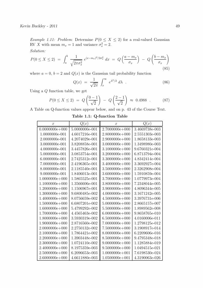
Kevin Buckley - 2011 49
Example 1.11: Problem: Determine P (0 ≤ X ≤ 2) for a real-valued GaussianRV X with mean mx = 1 and variance σ2
x = 2.
Solution:
P (0 ≤ X ≤ 2) =∫ b
a
1√
2πσ2x
e(x−mx)2/2σ2x dx = Q
(
a−mx
σx
)
− Q
(
b−mx
σx
)
(85)where a = 0, b = 2 and Q(x) is the Gaussian tail probability function
Q(x) =1√2π
∫ ∞
xeλ
2/2 dλ . (86)
Using a Q function table, we get
P (0 ≤ X ≤ 2) = Q
(
0− 1√2
)
− Q
(
2− 1√2
)
≈ 0.4988 . (87)
A Table on Q-function values appear below, and on p. 43 of the Course Text.
Table 1.1: Q-function Table
x Q(x) x Q(x)
0.0000000e+000 5.0000000e-001 2.7000000e+000 3.4669738e-0031.0000000e-001 4.6017216e-001 2.8000000e+000 2.5551303e-0032.0000000e-001 4.2074029e-001 2.9000000e+000 1.8658133e-0033.0000000e-001 3.8208858e-001 3.0000000e+000 1.3498980e-0034.0000000e-001 3.4457826e-001 3.1000000e+000 9.6760321e-0045.0000000e-001 3.0853754e-001 3.2000000e+000 6.8713794e-0046.0000000e-001 2.7425312e-001 3.3000000e+000 4.8342414e-0047.0000000e-001 2.4196365e-001 3.4000000e+000 3.3692927e-0048.0000000e-001 2.1185540e-001 3.5000000e+000 2.3262908e-0049.0000000e-001 1.8406013e-001 3.6000000e+000 1.5910859e-0041.0000000e+000 1.5865525e-001 3.7000000e+000 1.0779973e-0041.1000000e+000 1.3566606e-001 3.8000000e+000 7.2348044e-0051.2000000e+000 1.1506967e-001 3.9000000e+000 4.8096344e-0051.3000000e+000 9.6800485e-002 4.0000000e+000 3.1671242e-0051.4000000e+000 8.0756659e-002 4.5000000e+000 3.3976731e-0061.5000000e+000 6.6807201e-002 5.0000000e+000 2.8665157e-0071.6000000e+000 5.4799292e-002 5.5000000e+000 1.8989562e-0081.7000000e+000 4.4565463e-002 6.0000000e+000 9.8658765e-0101.8000000e+000 3.5930319e-002 6.5000000e+000 4.0160006e-0111.9000000e+000 2.8716560e-002 7.0000000e+000 1.2798125e-0122.0000000e+000 2.2750132e-002 7.5000000e+000 3.1908917e-0142.1000000e+000 1.7864421e-002 8.0000000e+000 6.2209606e-0162.2000000e+000 1.3903448e-002 8.5000000e+000 9.4795348e-0182.3000000e+000 1.0724110e-002 9.0000000e+000 1.1285884e-0192.4000000e+000 8.1975359e-003 9.5000000e+000 1.0494515e-0212.5000000e+000 6.2096653e-003 1.0000000e+001 7.6198530e-0242.6000000e+000 4.6611880e-003 1.0500000e+001 4.3190063e-026
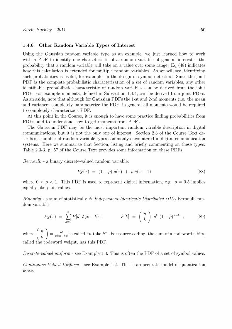
Kevin Buckley - 2011 50
1.4.6 Other Random Variable Types of Interest
Using the Gaussian random variable type as an example, we just learned how to workwith a PDF to identify one characteristic of a random variable of general interest – theprobability that a random variable will take on a value over some range. Eq (48) indicateshow this calculation is extended for multiple random variables. As we will see, identifyingsuch probabilities is useful, for example, in the design of symbol detectors. Since the jointPDF is the complete probabilistic characterization of a set of random variables, any otheridentifiable probabilistic characteristic of random variables can be derived from the jointPDF. For example moments, defined in Subsection 1.4.4, can be derived from joint PDFs.As an aside, note that although for Gaussian PDFs the 1-st and 2-nd moments (i.e. the meanand variance) completely parameterize the PDF, in general all moments would be requiredto completely characterize a PDF.
At this point in the Course, it is enough to have some practice finding probabilities fromPDFs, and to understand how to get moments from PDFs.
The Gaussian PDF may be the most important random variable description in digitalcommunications, but it is not the only one of interest. Section 2.3 of the Course Text de-scribes a number of random variable types commonly encountered in digital communicationsystems. Here we summarize that Section, listing and briefly commenting on these types.Table 2.3-3, p. 57 of the Course Text provides some information on these PDFs.
Bernoulli - a binary discrete-valued random variable:
PX(x) = (1− ρ) δ(x) + ρ δ(x− 1) (88)
where 0 < ρ < 1. This PDF is used to represent digital information, e.g. ρ = 0.5 impliesequally likely bit values.
Binomial - a sum of statistically N Independent Identically Distributed (IID) Bernoulli ran-dom variables:
PX(x) =n∑
k=0
P [k] δ(x− k) ; P [k] =
(
nk
)
ρk (1− ρ)n−k , (89)
where
(
nk
)
= n!k!(n−k)!
is called “n take k”. For source coding, the sum of a codeword’s bits,
called the codeword weight, has this PDF.
Discrete-valued uniform - see Example 1.3. This is often the PDF of a set of symbol values.
Continuous-Valued Uniform - see Example 1.2. This is an accurate model of quantizationnoise.

Kevin Buckley - 2011 51
Lognormal - the PDF of the natural log of a Gaussian random variable:
pX(x) =1√
2πσ2xe−(ln(x)−m)2/2σ2
u(x) , (90)
where σ2 and m are, respectively, the variance and mean of the Gaussian. We often takethe natural log of received data (e.g. to simplify subsequent detector computation). Thelognormal PDF also is used to model fading due to large reflectors.
Chi-squared with n degrees of freedom - the sum of the square of n zero-mean IID Gaussians.
pX(x) =1
2(n/2) Γ(n/2) σnx(n/2)−1 e−x/(2σ2) u(x) , (91)
where σ2 is the variance of the Gaussians and Γ(x) is the Gamma function. For noncoherentdetection we often sum the squares of IID Gaussians.
Noncentral chi-squared - the sum of the square of n equal-variance, uncorrelated Gaussianswith means mi; i = 1, 2, · · · , n:
pX(x) =1
2σ2
(
x
s2
)(n−2)/4
e−(s2+x)/(2σ2) I(n/2)−1
(
s
σ2
√x)
u(x) , (92)
where σ2 is the variance of the Gaussians, s =√
∑ni=1m
2i , and Iα(x) is the modified Bessel
function of the first kind and order α. For noncoherent detection we often sum the squaresof non-zero mean Gaussians.
Rayleigh - the square root of the sum of the square of two zero-mean IID Gaussians.
pX(x) =1
σ2x e−x2/(2σ2) u(x) , (93)
where σ2 is the variance of the two Gaussians. For noncoherent detection we often take thesquare root of the sum of the squares of zero-mean IID Gaussians.
Ricean - the square root of the sum of the square of two equal-variance, uncorrelated Gaus-sians with means mi; i = 1, 2:
pX(x) =1
2σ2e(x
2+s2)/(2σ2) I0
(
s x
σ2
)
u(x) , (94)
where σ2 is the variance of the two Gaussians and s =√
∑2i=1m
2i . For noncoherent detection
we often take the square root of the sum of the squares of nonzero-mean Gaussians.
Nakagami - a PDF which models signal fading that occurs for multipath scattering withrelatively larger time-delay spreads, with different clusters of reflected waves:
pX(x) =2
Γ(m)
(
m
Ω
)m
x2m−1 6−mx2/Ω u(x) , (95)
where Ω = EX2 and m = Ω2
E(X2−Ω)2.

Kevin Buckley - 2011 52
1.4.7 Bounds on Tail Probabilities
See pp. 56-63 of the Course Text for a complementary discussion on bounds on PDF tailprobabilities. As with the union bound introduced earlier, the bounds described here areuseful for performance analysis of coding schemes and decoding algorithms.
Consider a random variable X with mean mx, variance σ2x, and PDF illustrated below in
Figure 21(a). Consider a positive constant δ. Say we are interested in the probability
P (X ≥ mx + δ) = P (X −mx ≥ δ) , (96)
i.e. the probability that the random variable will be greater than or equal to δ above itsmean. If we know the PDF we can find this probability, exactly. Alternatively, we may lookfor a useful bound on this probability.
Chebyshev Inequality: For the two-sided tail probability illustrated in Figure 21(b),
P (|X −mx| ≥ δ) ≤ σ2x
δ2. (97)
Note that for symmetric PDF’s, we have P (X −mx ≥ δ) ≤ σ2x
2δ2.
Proof: Consider zero mean Y = X −mx. The Chebyshev inequality in terms of Y is
P (|Y | ≥ δ) ≤ σ2x
δ2. (98)
As illustrated in Figure 22(a), letg(Y ) =
1 |Y | ≥ δ0 otherwise
. (99)
Let pY (y) denote the PDF of Y . Then,
Eg(Y ) =∫ ∞
−∞g(y) pY (y) dy =
∫
|y|≥δ1 pY (y) dy = P (|Y | ≥ δ) . (100)
Since g(Y ) ≤(
Yδ
)2for all Y , we have
Eg(Y ) ≤ E(
Y
δ
)2
=EY 2
δ2=
σ2x
δ2. (101)
So,P (|X −mx| ≥ δ) ≤ σ2
x
δ2. (102)
This derivation of the Chebyshev inequality (bound) leads to the following tighter bound.
µx
µ + δx
p( )x
x
(b)x
µ − δ µx
µ + δx
p( )x
x
(a)
Figure 21: (a) A tail probability; (b) a two-sided tail probability for the Chebyshev inequality.
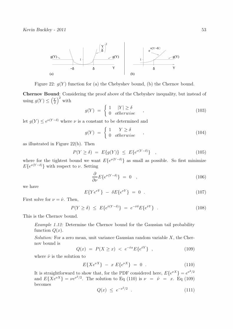
Kevin Buckley - 2011 53
δY
2
−δ δ
g(Y)g(Y)
Y
Yν( −δ)e
δ
g(Y)
Y
1
(a) (b)
1
Figure 22: g(Y ) function for (a) the Chebyshev bound, (b) the Chernov bound.
Chernov Bound: Considering the proof above of the Chebyshev inequality, but instead of
using g(Y ) ≤(
Yδ
)2with
g(Y ) =
1 |Y | ≥ δ0 otherwise
, (103)
let g(Y ) ≤ eν(Y−δ) where ν is a constant to be determined and
g(Y ) =
1 Y ≥ δ0 otherwise
, (104)
as illustrated in Figure 22(b). Then
P (Y ≥ δ) = Eg(Y ) ≤ Eeν(Y−δ) , (105)
where for the tightest bound we want Eeν(Y−δ) as small as possible. So first minimizeEeν(Y−δ) with respect to ν. Setting
∂
∂νEeν(Y−δ) = 0 , (106)
we haveEY eνY − δEeνY = 0 . (107)
First solve for ν = ν. Then,
P (Y ≥ δ) ≤ Eeν(Y−δ) = e−νδEeνY . (108)
This is the Chernov bound.
Example 1.12: Determine the Chernov bound for the Gaussian tail probabilityfunction Q(x).
Solution: For a zero mean, unit variance Gaussian random variable X , the Cher-nov bound is
Q(x) = P (X ≥ x) < e−νxEeνY , (109)
where ν is the solution to
EXeνX − x EeνX = 0 . (110)
It is straightforward to show that, for the PDF considered here, EeνX = eν2/2
and EXeνX = νeν2/2. The solution to Eq (110) is ν = ν = x. Eq (109)
becomesQ(x) ≤ e−x2/2 . (111)
Kevin Buckley - 2011 54
1.4.8 Weighted Sums of Multiple Random Variables
Let Xi; i = 1, 2, · · · , N be N random variables and ci; i = 1, 2, · · · , N be constants. Considerthe following linear combination (weighted sum) of the random variables:
Y =N∑
i=1
ci Xi = cT X , (112)
where X = [X1, X2, ..., Xn]T and c = [c1, c2, ..., cn]
T . The following results are important tokeep in mind.
1. The mean of Y :
EY = my = E
N∑
i=1
ci Xi
=N∑
i=1
ci EXi =N∑
i=1
ci mxi= cT mx , (113)
where mx is the mean vector of random vector X . That is, the mean of the weightedsum is the weighted sum of the means. This is a direct consequence of linearity of theexpectation operator. Note that no restrictions are placed on the Xi.
2. The variance of Y : First, let the Xi be uncorrelated. Then,
σ2y =
N∑
i=1
|ci|2 σ2xi
. (114)
So, under the uncorrelated assumption stated above, the variance of the weighted sumis the magnitude-squared-weighted sum of the variances.
Now consider general Xi (i.e. possibly correlated). Let Cx be the covariance matrix ofX . Then
σ2y = cT Cx c∗ . (115)
3. The PDF of Y : Let the Xi be statistically independent. Let Yi = ci Xi. Note thatpYi
(yi) =1|ci|
pXi(yi/ci). Then,
pY (y) = pY1(y) ∗ pY2
(y) ∗ · · · ∗ pYN(y) . (116)
Basically, for independent random variables, the PDF of the sum is the convolution ofthe PDF’s.
4. Gaussian Xi: If the Xi are Gaussian, then so is Y . This is true even if the Xi arecorrelated (i.e. for Gaussian not statistically independent).
Since the PDF of a Gaussian RV is completely characterized by its mean and variance,for Gaussian Xi we can easily determine pY (y) (i.e. without convolving the individualXi PDF’s), and we can do this even if the Xi are correlated. We just determine mY
and σ2y , using rules 1. & 2. stated above, and plug them into the Gaussian PDF
expression.
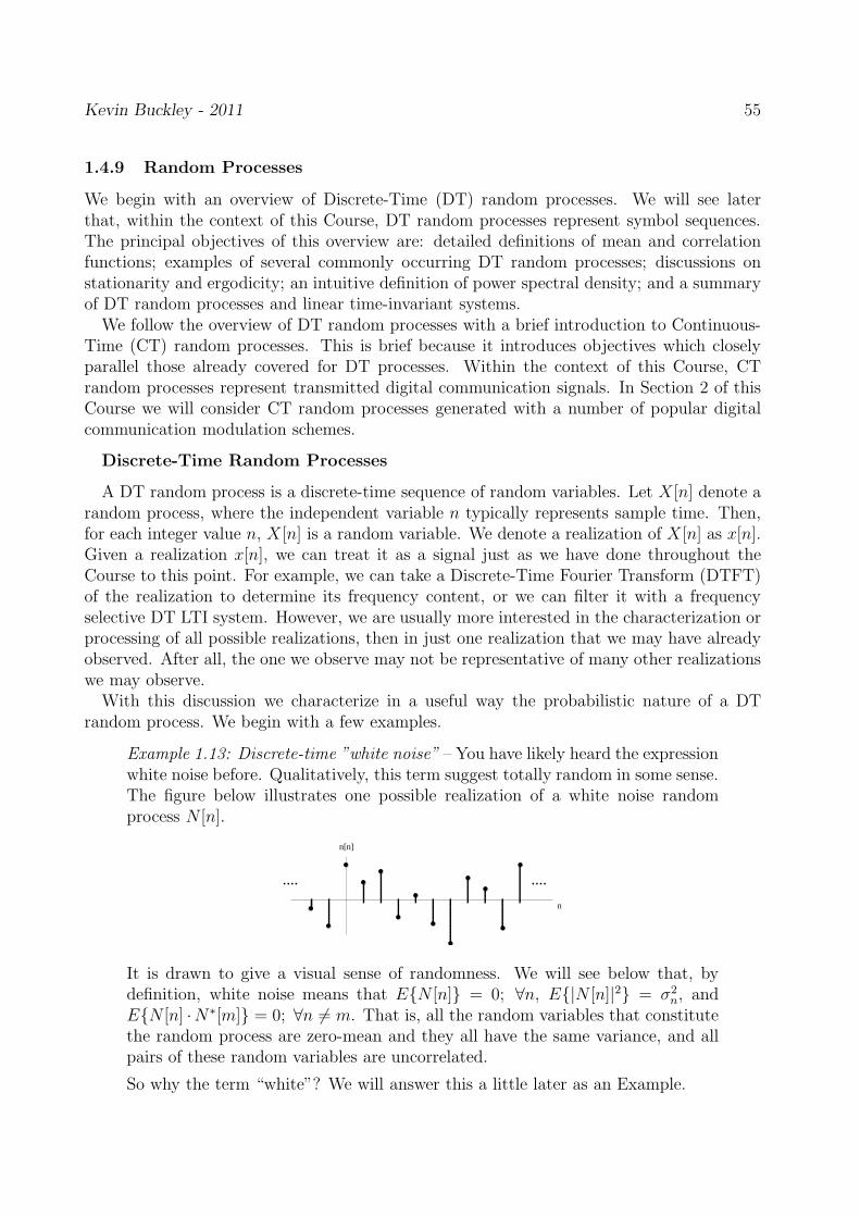
Kevin Buckley - 2011 55
1.4.9 Random Processes
We begin with an overview of Discrete-Time (DT) random processes. We will see laterthat, within the context of this Course, DT random processes represent symbol sequences.The principal objectives of this overview are: detailed definitions of mean and correlationfunctions; examples of several commonly occurring DT random processes; discussions onstationarity and ergodicity; an intuitive definition of power spectral density; and a summaryof DT random processes and linear time-invariant systems.
We follow the overview of DT random processes with a brief introduction to Continuous-Time (CT) random processes. This is brief because it introduces objectives which closelyparallel those already covered for DT processes. Within the context of this Course, CTrandom processes represent transmitted digital communication signals. In Section 2 of thisCourse we will consider CT random processes generated with a number of popular digitalcommunication modulation schemes.
Discrete-Time Random Processes
A DT random process is a discrete-time sequence of random variables. Let X [n] denote arandom process, where the independent variable n typically represents sample time. Then,for each integer value n, X [n] is a random variable. We denote a realization of X [n] as x[n].Given a realization x[n], we can treat it as a signal just as we have done throughout theCourse to this point. For example, we can take a Discrete-Time Fourier Transform (DTFT)of the realization to determine its frequency content, or we can filter it with a frequencyselective DT LTI system. However, we are usually more interested in the characterization orprocessing of all possible realizations, then in just one realization that we may have alreadyobserved. After all, the one we observe may not be representative of many other realizationswe may observe.
With this discussion we characterize in a useful way the probabilistic nature of a DTrandom process. We begin with a few examples.
Example 1.13: Discrete-time ”white noise” – You have likely heard the expressionwhite noise before. Qualitatively, this term suggest totally random in some sense.The figure below illustrates one possible realization of a white noise randomprocess N [n].
n
.... ....
n[n]
It is drawn to give a visual sense of randomness. We will see below that, bydefinition, white noise means that EN [n] = 0; ∀n, E|N [n]|2 = σ2
n, andEN [n] ·N∗[m] = 0; ∀n 6= m. That is, all the random variables that constitutethe random process are zero-mean and they all have the same variance, and allpairs of these random variables are uncorrelated.
So why the term “white”? We will answer this a little later as an Example.
Kevin Buckley - 2011 56
Example 1.14: A complex sinusoidal random process – A complex sinusoidalrandom process X [n] has the form
X [n] = A ej(Ωn+Φ)
where in general A, Ω and Φ are random variables. A realization of X [n] will be acomplex sinusoid, whose magnitude, frequency and phase will be some realizationof, respectively, A, Ω and Φ.
Consider, for example, the case where A and Ω are constant (i.e. known, non-random), and Φ is uniformly distributed with PDF
pΦ(φ) =
12π
0 ≤ φ < 2π0 otherwise
The mean of each random variable that constitutes this random process is
mx[n] = EX [n] = EA ej(Ωn+Φ) = AejΩn EejΦ
= AejΩn 1
2π
∫ 2π
0ejφ dφ = 0 .
In general, the means of the random variables are different at different times.This one has constant (zero) mean for all time, i.e. mx[n] = mx = 0.
The correlation between any two random variables, say at times n and m, is
EX [m] X∗[n] = EAej(Ωm+Φ) Ae−j(Ωn+Φ) = A2ejΩ(m−n) EejΦe−jΦ= A2ejΩ(m−n) E1 = A2 ejΩ(m−n)
We see from this expression that form = n, i.e. when we are correlating a randomsample with itself, we just get the variance of that random variable, σ2
x[n] = A2.
Note that this is not a function of n, i.e. σ2x[n] = σ2
x = A2. Also note thatthe correlation between two random variables, at times n and m, is a function ofonly the distance in time m− n between them. It is not a function of where thesamples are in time.
Partial Characterizations of DT Random Processes: The Mean & Correlation Functions
A complete probabilistic description of a DT random process consists of the set of all jointPDF’s of all combinations of the random variables that constitutes the random process.In many situations all of this information is not available, and in most situations it is notnecessary for the effective processing of the random process. An effective, common andsomewhat general representation of random processes is in terms of moments. Althoughhigher order moments are sometimes used, in the vast majority of applications using justthe 1-st and 2-nd order moments of a random process can be effective. Here we describe the1-st and 2-nd order moment descriptions of DT random processes.

Kevin Buckley - 2011 57
• The Mean Function: The mean function of a DT random process X [n] is defined as
mx[n] = EX [n] =∫ ∞
−∞x[n] pX[n](x[n]) dx[n] ; ∀ n . (117)
It is the function of means of all the random variables that constitute the randomprocess. In general, as the notation mx[n] implies, the mean is time varying.
• The AutoCorrelation Function (ACF): The autocorrelation function of a DT randomprocess X [n] is defined as
RX [m,n] = EX [m]X∗[n] =∫ ∞
−∞
∫ ∞
−∞x[m] x∗[n] pX[m],X[n](x[m], x[n]) dx[m] dx[n] ; ∀m,n.
(118)It is the function of all correlations between the random variables that constitute therandom process. It is a two dimensional function of the times m and n of the twosamples which are being correlated.
• The Autocovariance Function: The autocovariance function of a DT random processX [n] is defined as
CX [m,n] = E(X [m]−mX[m]) (X [n]−mx[n])∗ (119)
= RX [m,n] − mx[m] ·m∗x[n] . (120)
Eq (120) can be derived from Eq (119) using the linearity property of the expectation.Note that if the random process is zero-mean for all time, then CX [m,n] = RX [m,n].
Note that although these function are defined in terms of PDF’s, they will usually be iden-tified by other means such as those considered later in this Course. For example, if youwanted to determine (i.e. estimate) them from data, you might substitute the ensembleaverages (expectations) given above with average over available data.
One way that random processes are characterized is in terms of properties of their meanand correlation functions. We now identify the most common category of DT random pro-cesses.
Wide-Sense Stationary DT Processes
Qualitatively, stationarity of a random process means that its probabilistic characteristicsdo not change with time. There are different types of stationarity corresponding to differentcharacteristics.
Stationarity in the mean means
mx[n] = mx . (121)
That is, the mean is not a function of time n.Wide-sense stationarity means stationarity in the mean plus
RX [n, n− l] = EX [n] X∗[n− l] = RX [l] . (122)
That is, in addition to the mean is not being function of time n, the autocorrelation functionis not a function of time n, but only a function of the difference in time l between samplesbeing correlated. This distance, l, is termed the lag.

Kevin Buckley - 2011 58
Example 1.15: Discrete-Time White Noise – In Example 1.13, DT white noisewas described as a DT random process, say N [n], with EN [n] = 0; ∀n,E|N [n]|2 = σ2
n; ∀n, and EN [n] · N∗[m] = 0; ∀n 6= m. We now recognizethat with these properties, white noise is zero mean, i.e.
mn[n] = mn = 0 , (123)
with autocorrelation function
RN [n, n− l] = RN [l] = σ2n δ[l] . (124)
So, white noise is wide-sense stationary.
Example 1.16: A complex sinusoidal random process – In Example 1.14 we con-sidered the DT random process
X [n] = A ej(Ωn+Φ)
where A and Ω are constant, and Φ is uniformly distributed over values 0 ≤ φ <2π.
We observed that mn[n] = 0, i.e. we can now say that the random processhas zero mean. We also concluded that EX [m] X∗[n] = A2 ejΩ(m−n). Thatis, the autocorrelation function is RX [n, n − l] = RX [l] = A2 ejΩl. So theautocorrelation function is a function of only the lag (the distance in time betweenthe random variables).
As in Example 1.15, this random process is wide-sense stationary.
Example 1.17: Another complex sinusoidal random process – As in Example 1.16,consider
X [n] = A ej(Ωn+Φ)
where Ω is still constant and Φ is uniformly distributed over values 0 ≤ φ < 2π,but now let A be a Gaussian random variable with zero mean and variance σ2
a.Assume that A and φ are statistically independent. Determine the mean andautocorrelation functions. Is this random process wide-sense stationary?
Solution: Note that pA,Φ(a, φ) = pA(a) · pΦ(φ), since A and Φ are statisticallyindependent The mean function is
mx[n] =∫ ∞
−∞
∫ ∞
−∞x[n] pA,Φ(a, φ) da dφ = ejΩn
∫ ∞
−∞
∫ ∞
−∞ejφpΦ(φ) dφ ·
∫ ∞
−∞a pA(a) da
= ejΩn 1
2π
∫ 2π
0ejφ dφ ·
∫ ∞
−∞a
1√
2πσ2a
e−a2/2σ2a da = 0.
That is, both integrals in the last line are zero. This random process is zero-mean.
The autocorrelation function can be shown to be
RX [n, n− l] = RX [l] = σ2a ejΩl .
So this DT sinusoidal random process is also wide-sense stationary.

Kevin Buckley - 2011 59
Not all sinusoidal random processes are wide-sense stationary. The above examples wereselected because we are only interested in wide-sense stationary processes in this overview.
Example 1.18: Additive White Gaussian Noise (AWGN) – A very common typeof random process, often observed at the sampled output of a sensor (or thesampled output of a preamplifier connected directly to a sensor) when there isno signal received by the sensor, is AWGN.
White means that all the sample are zero-mean, uncorrelated with one another,and all have the same variance (i.e. see Example 1.13).
Gaussian means that each sample is Gaussian distributed. Let N [n] denote theAWGN process. Then,
pN [n](n[n]) =1
√
2πσ2n
e−n2[n]/2σ2n (125)
and since uncorrelated Gaussian random variables are statistically independentthe joint PDF of any set of samples is the product of their individual PDF’s,each of the Eq (125) form. So for this random process we know the completestatistical description.
Additive implies that, in the presence of a signal, the noise is added to it. It alsotypically implies that the signal, if also a random process, is uncorrelated withthe noise. Let X [n] = S[n] +N [n] be the sampled sensor output, where S[n] is asignal and N [n] is AWGN. Then it is easy to show that, since S[n] and N [n] areuncorrelated,
RX [l] = RS[l] + RN [l] ∀ l ,
where we already know that RN [l] = σ2n δ[l].
Signal-to-Noise Ratio (SNR): For wide-sense stationary random processes, as with otherpower signals, SNR is defined as the ratio of the signal power to the noise power. For arandom process X [n] = S[n] + N [n], consisting of wide-sense stationary signal S[n] andnoise N [n], the SNR is
SNR =RS[0]
RN [0]; SNRdb = 10 log10(SNR) . (126)
Example 1.19: Let X [n] = S[n] + N [n], where the signal S[n] is a complexsinusoidal process as described in Example 1.17, andN [n] is AWGN with varianceσ2n. Let σ
2a = 20 and σ2
n = 10. The SNR is
SNR =RS[0]
RN [0]=
σ2s
σ2n
=20
10= 2; SNRdb ≈ 3 dB .

Kevin Buckley - 2011 60
Temporal Averages
Temporal averages are averages over time of one realization of a random process. This isas opposed to the expectation operator which is an ensemble average (i.e. it averages overrealizations). For example, some time averaged means are
< x[n] >n0,n1=
1
n1 − n0 + 1
n1∑
n=n0
x[n] (127)
< x[n] > = limM→∞
1
2M + 1
M∑
n=−M
x[n] . (128)
Ergodicity
Qualitatively, a random process is ergodic if temporal averages give ensemble averages.Ergodic in the mean:
mx = < x[n] > = EX [n] . (129)
Ergodic in the autocorrelation:
RX [l] = < x[n] x∗[n− l] > = limM→∞
1
2M + 1
M∑
n=−M
x[n] x∗[n− l] . (130)
Note that the right side of Eq(130) is called a deterministic correlation. For a random processto be ergodic in some sense, it must be stationary in that sense.

Kevin Buckley - 2011 61
Comment on Estimating the Mean and ACF
Suppose we need to know the mean function and ACF of a random process, but we haveonly one realization of it over only times n = 0, 1, · · · , N − 1. Can we use temporal averagesto derive estimates? In general, the answer is no since if the mean and ACF change overtime, we can’t average over time to estimate them. So we need the random process to bewide-sense stationary. But this is not enough, we also need to be able to assume that therandom process is wide-sense ergodic.
Example 1.20 - Given a single finite-duration realization x[n]; n = 0, 1, · · · , N−1of a wide-sense stationary and ergodic random process X [n], using Eqs (128, 130)as guidance, suggest equations for estimating the mean and ACF.
Solution:
mx =1
N
N−1∑
n=0
x[n]
RX [l] =
1N−l
=∑N−1
n=l x[n] x∗[n− l] 0 ≤ l ≤ N − 1
R∗X [−l] −N + 1 ≤ l ≤ −1
0 otherwise

Kevin Buckley - 2011 62
Power Spectral Density (PSD) of a Wide-Sense Stationary Random Process
Let X [n] be a wide-sense stationary random process, and let x[n] be a realization. Denotethe Discrete-Time Fourier Transform (DTFT) of a 2N + 1 sample window of the randomprocess as
XN(ej2πf) =
N∑
n=−N
x[n] e−jn2πf . (131)
The Power Spectral Density (PSD) is defined as
SX(f) = limN−→∞
1
2N + 1E|XN(e
j2πf)|2 . (132)
The PSD is the expected value of the magnitude-squared of the DTFT of a window ofthe random process, as the window width approaches infinity. This definition of the PSDcaptures what we want as a measure of the frequency content of a random discrete-timesequence.
Let’s take an alternative view of SX(f). First consider the term on the right of the previousequation, without the limit and expectation:
1
2N + 1|XN(e
j2πf)|2 =1
2N + 1
N∑
n=−N
x[n] e−jn2πfN∑
l=−N
x∗[l] ejl2πf
=1
2N + 1
N∑
n=−N
N∑
l=−N
x[n] x∗[l] e−j(n−l)2πf
=1
2N + 1
N∑
n=−N
n+N∑
m=n−N
x[n] x∗[n−m] e−jm2πf .
Taking the expected value, we have
1
2N + 1E|XN(e
j2πf)|2 =1
2N + 1
N∑
n=−N
n+N∑
m=n−N
φxx[m] e−jm2πf . (133)
Now, taking the limit as N −→ ∞, we have
SX(f) = limN−→∞
1
2N + 1E|XN(e
j2πf)|2
= limN−→∞
1
2N + 1
N∑
n=−N
∞∑
m=−∞
RX [m] e−jm2πf
=∞∑
m=−∞
RX [m] e−jm2πf limN−→∞
1
2N + 1
N∑
n=−N
1
=∞∑
m=−∞
RX [m] e−jm2πf .

Kevin Buckley - 2011 63
Thus, the power PSD and the ACF of a wide-sense stationary random process form theDTFT pair
SX(f) =∞∑
l=−∞
RX [l] e−jl2πf (134)
RX [l] =∫ 1/2
−1/2SX(f) e
jl2πf df . (135)
Example 1.21 - Given the ACF RX [m] = σ2x 0.5|l| of a wide-sense stationary
random process X [n], determine and sketch the PSD SX(f).
Solution:
Example 1.22 - Complex sinusoidal random signals in uncorrelated noise.
Solution:
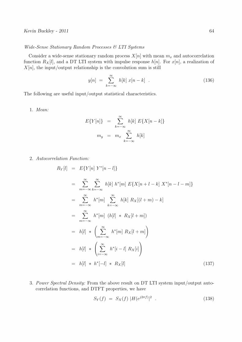
Kevin Buckley - 2011 64
Wide-Sense Stationary Random Processes & LTI Systems
Consider a wide-sense stationary random process X [n] with mean mx and autocorrelationfunction RX [l], and a DT LTI system with impulse response h[n]. For x[n], a realization ofX [n], the input/output relationship is the convolution sum is still
y[n] =∞∑
k=−∞
h[k] x[n− k] . (136)
The following are useful input/output statistical characteristics.
1. Mean:
EY [n] =∞∑
k=−∞
h[k] EX [n− k]
my = mx
∞∑
k=−∞
h[k]
2. Autocorrelation Function:
RY [l] = EY [n] Y ∗[n− l]
=∞∑
m=−∞
∞∑
k=−∞
h[k] h∗[m] EX [n+ l − k] X∗[n− l −m]
=∞∑
m=−∞
h∗[m]∞∑
k=−∞
h[k] RX [(l +m)− k]
=∞∑
m=−∞
h∗[m] (h[l] ∗ RX [l +m])
= h[l] ∗(
∞∑
m=−∞
h∗[m] RX [l +m]
)
= h[l] ∗
∞∑
i=−∞
h∗[i− l] RX [i]
= h[l] ∗ h∗[−l] ∗ RX [l] (137)
3. Power Spectral Density: From the above result on DT LTI system input/output auto-correlation functions, and DTFT properties, we have
SY (f) = SX(f) |H(ej2πf)|2 . (138)

Kevin Buckley - 2011 65
Example 1.23: Let wide-sense stationary input X [n] be zero-mean white noisewith variance σ2
n, and DT LTI system impulse response be h[n] = δ[n] + δ[n− 1].Determine the ACF and PSD of the output Y [n].
Solution:
Example 1.24: Let h[n] = 1N(u[n]−u[n−N ]), andX [n] be a wide-sense stationary
complex sinusoidal process with RX [l] = σ2X ejω0l where |ω0| ≤ π. Determine the
ACF and PSD of the output Y [n].
Solution:

Kevin Buckley - 2011 66
Continuous-Time (CT) Random Processes
For continuous-time (CT) wide-sense stationary random process X(t), the mean, autocor-relation, and autocovariance functions are defined, respectively, as
mx = EX(t) (139)
RX(τ) = EX(t) X∗(t− τ) (140)
CX(τ) = E(X(t)−mx) (X(t− τ)−mx)∗ = RX(τ)− |mx|2 . (141)
Note that, because the process is wide-sense stationary, these functions are not a functionof time t. That is, the mean is constant, and the correlation and covariance functions arefunctions of only the distance in time τ between the random variables being producted. Oftena wide-sense stationary random process is zero-mean. Then, mx = 0 and RX(τ) = CX(τ),and we use the terms correlation and covariance interchangeably. Zero mean processes areeasier to work with, so that in practice if a process is not zero mean, the mean is oftenfiltered out. The power spectral density (PSD) of a CT wide-sense stationary process is3
SX(f) =∫ ∞
−∞RX(τ) e
−j2πfτ dτ RX(τ) =∫ ∞
−∞SX(f) e
j2πfτ df (143)
i.e. the continuous-time Fourier transform (CTFT) of the autocorrelation function.Consider a wide-sense stationary random process X(t) as the input to a linear time-
invariant (LTI) system (e.g. a transmitted signal through a channel, or a received signalthrough a receiver filter). Denote the LTI system impulse response h(t) and correspondingfrequency response H(f). The output Y (t) is also wide-sense stationary with
my = mx
∫ ∞
−∞h(t) dt (144)
RY (τ) = RX(τ) ∗ h(τ) ∗ h∗(−τ) (145)
SY (f) = SX(f) |H(f)|2 . (146)
3As in the Course Text, here we express the PSD as a function of frequency f is Hertz. The autocor-relation/PSD relationship is the continuous-time FT (CTFT) as shown. More conventionally, the PSD weexpressed as a function of angular frequency ω, in which case the CTFT pair is
SX(ω) =
∫
∞
−∞
RX(τ) e−jωτ dτ ; RX(τ) =1
2π
∫
∞
−∞
SX(ω) ejωτ dω . (142)

Kevin Buckley - 2011 67
Real-Valued Bandpass (Narrowband) Signals & Their Lowpass Equivalents
This topic is covered on Sections 2.9 of the Course Text. Within the context of this Course,real-valued bandpass random signals represent modulated carriers and additive noise.
Recall from Subsection 1.2.1 of these Course Notes that given a real-valued continuous-time bandpass signal x(t) with Hilbert transform x(t) and lowpass equivalent xl(t), we havethat
xl(t) = [x(t) + j x(t)] e−j2fct (147)
where fc is the center frequency of the bandpass signal (i.e. see Eqs (11,14) and Figure8(a) from Lecture 1). Let X(t) be a real-valued bandpass CT wide-sense stationary randomprocess, such that its power spectral density Sx(f) = 0 for |(f − fc)| > B and B << fc. Thecorrelation function
RX(τ) = EX(t) X(t− τ) =∫ ∞
−∞Sx(f) e
j2πfτ df (148)
is real-valued. Since Rx(τ) is a real-valued bandpass function, it has a “lowpass equivalent”which we will denote as R
′
x(τ), i.e.
R′
X(τ) = [RX(τ) + j RX(τ)] e−j2fct (149)
where RX(τ) is the Hilbert transform of RX(τ). Then, also from Section 1.2.1 of the CourseNotes, we have that the CTFT of R
′
X(τ) and the PSD of X(t) are related as
SX(f) =1
2[S
′
X(f − fc) + S′
X(−f − fc)] (150)
(i.e. see Eq (13) of Lecture 1, noting that PSDs are real-valued).The lowpass equivalent process of X(t) is defined as
Xl(t) = Xi(t) + j Xq(t) , (151)
where Xi(t) andXq(t) are the in-phase and quadrature components ofX(t) (i.e. as generatedas illustrated in Figure 8(b) of Lecture 1 and Figure 2.1-6(b) of the Course Text).
In the Course Text (i.e. Eq (2.9-12) it is shown that the correlation function of the lowpassequivalent process of X(t) is
RXl(τ) = 2 [RX(τ) + j RX(τ)] e
−j2fct (152)
= 2 R′
X(τ) . (153)
So, the correlation function that we see at the receiver (that is, at the output of a quadraturereceiver) is twice that of the lowpass equivalent R
′
X(τ) of the correlation function of thebandpass signal X(t). So, the PSD of the lowpass equivalent process Xl(t) and the CTFT ofthe lowpass equivalent of the bandpass correlation function are related as
SXl(f) = 2 S
′
X(f) (154)
and the PSDs of X(t) and Xl(t) are related as
SX(f) =1
4[SXl
(f − fc) + SXl(−f − fc)] . (155)
Note the 14factor in this relationship. Figure 23 illustrates this relationship.
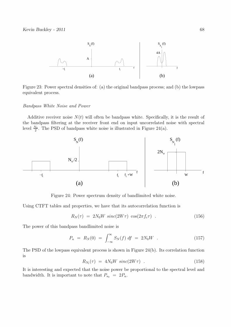
Kevin Buckley - 2011 68
S (f)X
l
S (f)X
(b)(a)
f−f fcc
A
f
4A
Figure 23: Power spectral densities of: (a) the original bandpass process; and (b) the lowpassequivalent process.
Bandpass White Noise and Power
Additive receiver noise N(t) will often be bandpass white. Specifically, it is the result ofthe bandpass filtering at the receiver front end on input uncorrelated noise with spectrallevel N0
2. The PSD of bandpass white noise is illustrated in Figure 24(a).
N /2o
2No
fc−fc
(b)(a)
f
S (f) S (f)l
N N
fc Wf +W
Figure 24: Power spectrum density of bandlimited white noise.
Using CTFT tables and properties, we have that its autocorrelation function is
RN(τ) = 2N0W sinc(2Wτ) cos(2πfcτ) . (156)
The power of this bandpass bandlimited noise is
Pn = RN(0) =∫ ∞
−∞SN (f) df = 2N0W . (157)
The PSD of the lowpass equivalent process is shown in Figure 24(b). Its correlation functionis
RNl(τ) = 4N0W sinc(2Wτ) . (158)
It is interesting and expected that the noise power be proportional to the spectral level andbandwidth. It is important to note that Pnl
= 2Pn.

Kevin Buckley - 2011 69
Digitally Modulated Signals
In Section 2 of this Course (and Chapter 3 of the Course Text) we will discuss digitallymodulated signals (i.e. signals transmitted in digital communication systems). These areCT real-valued bandpass signals, and they are random since they are modulated by randominformation sequences. As we will see, these CT digitally modulated signals are not Wide-Sense Stationary (WSS). They are what we call cyclostationary signals. Though they arenot WSS, we will be able to characterize them using an extension of the ACF and PSDdefined above for WSS processes.
We will need to get a feel for the spectral content of digitally modulated signals so thatwe can understand the channel bandwidth requirements for their transmission. We willtackle this issue later in Section 2 of this Course. Section 3.4 of the Course Text discussesfrequency characteristics of digitally modulated signals. That discussion is somewhat generaland challenging. We will simplify that discussion so as to identify more basic and targetedresults.
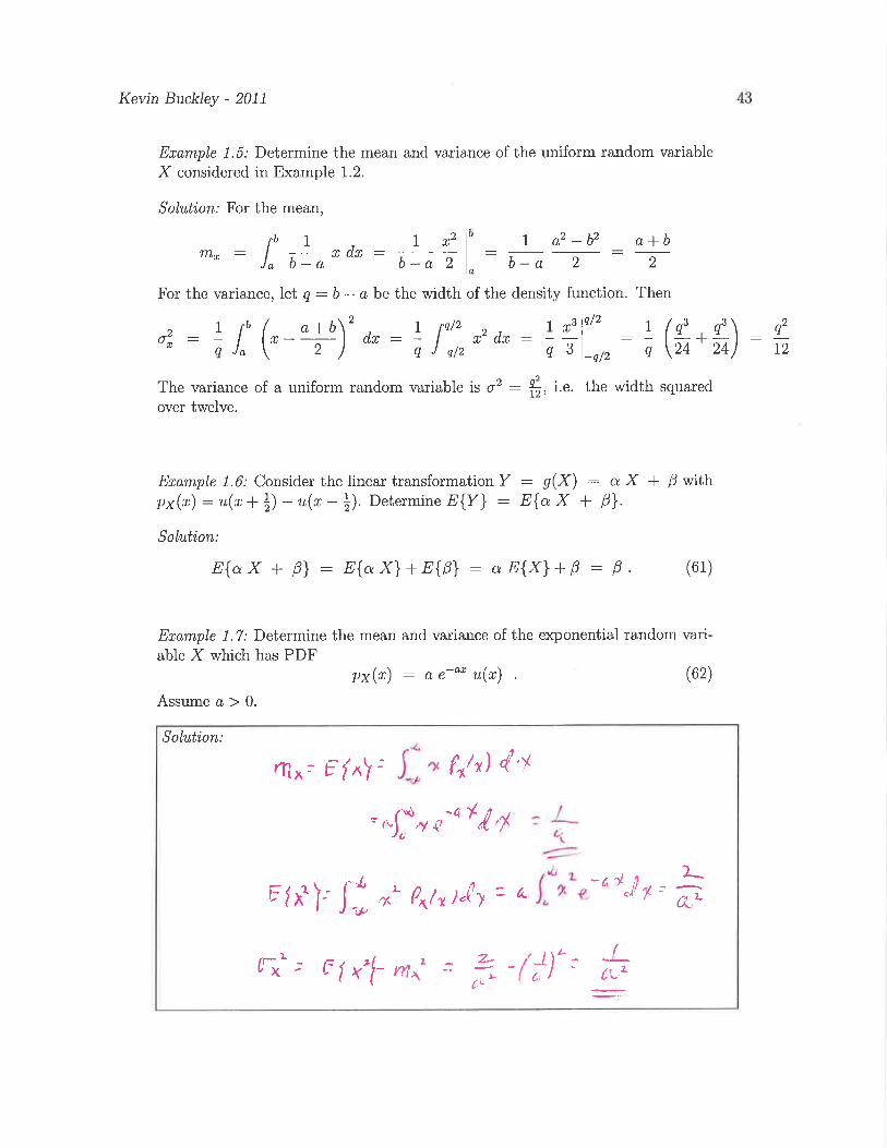

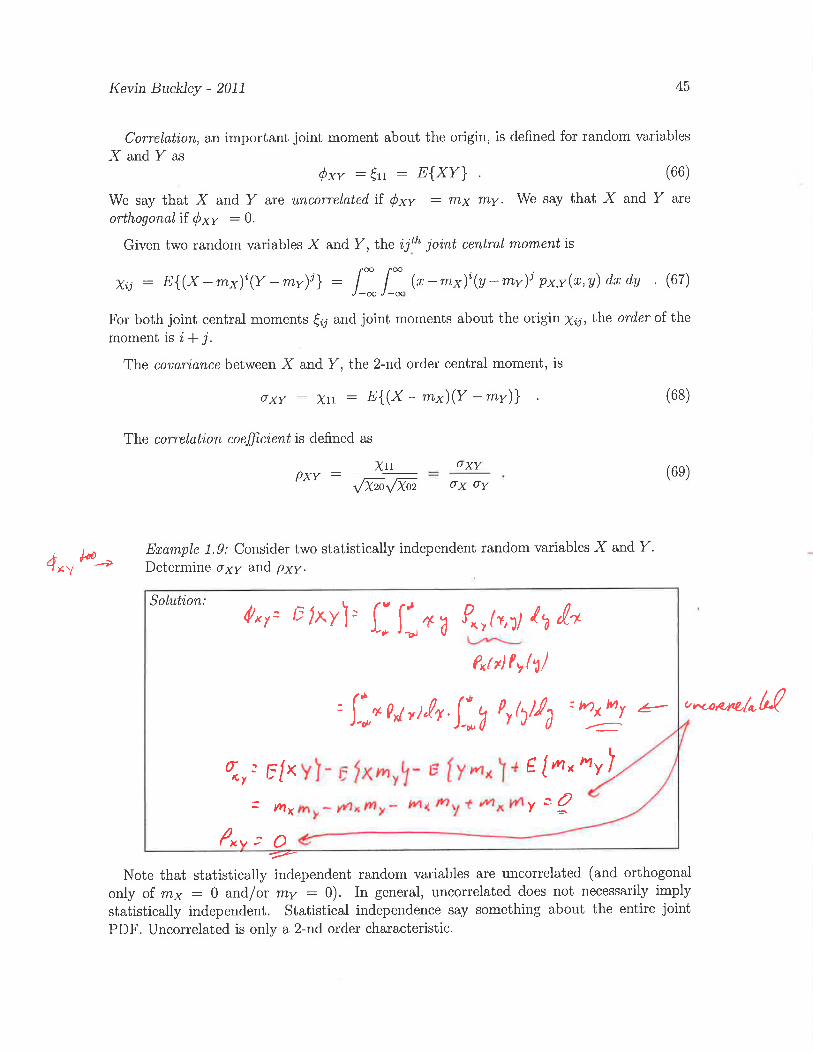

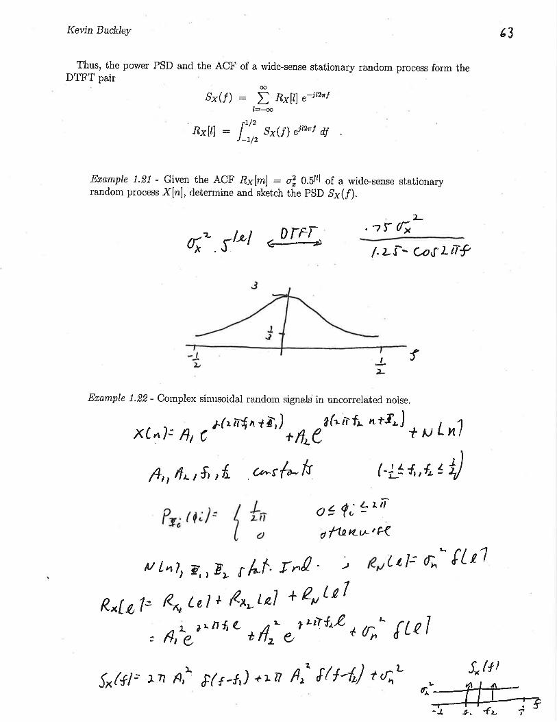


Kevin Buckley - 2011 68
ECE8700Communication Systems Engineering
Villanova UniversityECE Department
Prof. Kevin M. Buckley
Lecture 4
(b) M−16 QAM on rectangular grid(a) M=16 QAM on circular grid

Kevin Buckley - 2011 69
Contents
2 Representation of Digitally Modulated Signals 702.1 PAM - Memoryless and Linear . . . . . . . . . . . . . . . . . . . . . . . . . . 722.2 Phase Modulated Signals - Memoryless & Linear . . . . . . . . . . . . . . . . 742.3 Quadrature Amplitude Modulation (QAM) - Memoryless & Linear . . . . . 762.4 Notes on Multidimensional Modulation Schemes . . . . . . . . . . . . . . . . 78
2.4.1 Orthogonal Signal . . . . . . . . . . . . . . . . . . . . . . . . . . . . . 782.4.2 Frequency Shift Keying (FSK) . . . . . . . . . . . . . . . . . . . . . . 792.4.3 Biorthogonal Signaling . . . . . . . . . . . . . . . . . . . . . . . . . . 792.4.4 Binary Coded Modulation (BCM) . . . . . . . . . . . . . . . . . . . . 80
2.5 Several Modulation Schemes with Memory . . . . . . . . . . . . . . . . . . . 812.5.1 Differential PSK (DPSK) . . . . . . . . . . . . . . . . . . . . . . . . . 812.5.2 Partial Response Signaling (PRS) . . . . . . . . . . . . . . . . . . . . 832.5.3 Continuous-Phase Modulation (CPM) . . . . . . . . . . . . . . . . . 84
2.6 Spectral Characteristics of Digitally Modulated Signals . . . . . . . . . . . . 86
List of Figures
25 A PAM signal and its lowpass equivalent for an M = 4 symbol scheme. . . . 7226 PAM signal space representation for M = 2, M = 4. . . . . . . . . . . . . . . 7327 A PSK signal and its lowpass equivalent for an M = 4 symbol scheme. . . . 7428 PSK signal space representation for M = 2, M = 4. . . . . . . . . . . . . . . 7529 A QAM signal and its lowpass equivalent for an M = 4 symbol scheme. . . . 7630 Signal space representations for two QAM schemes. . . . . . . . . . . . . . . 7731 An example of the lowpass equivalent of a possible BCM symbol. . . . . . . 8032 An example of DPSK. . . . . . . . . . . . . . . . . . . . . . . . . . . . . . . 8233 NRZI coding. . . . . . . . . . . . . . . . . . . . . . . . . . . . . . . . . . . . 8234 Trellis diagram representation of DPSK. . . . . . . . . . . . . . . . . . . . . 8335 PRS example (from Problem 4.21 of the Course Text). . . . . . . . . . . . . 8336 PRS trellis diagram (for Problem 4.21 of the Course Text). . . . . . . . . . . 8437 Common continuous phase modulation scheme pulse shapes. . . . . . . . . . 8538 Several pulse shapes and corresponding spectral shapes: (a) rectangular; (b)
raised cosine; (c) ideal sinc. . . . . . . . . . . . . . . . . . . . . . . . . . . . 90

Kevin Buckley - 2011 70
2 Representation of Digitally Modulated Signals
This Section of the Course Notes corresponds to selected topics from Chapter 3 of theCourse Text. The objective here is to classify digital modulation schemes and introduceseveral schemes which will be considered later in the Course. We will describe these in termsof both their symbol waveforms (i.e. signals) their signal space representations. We will alsoconsider the frequency content of these signals.
The digital communication problem is to transmit and receive a random binary informationsequence an, where here n represents the discrete-time bit index. Digital modulation is themapping of this binary sequence to a transmitted waveform s(t) that carries this sequence.Conceptually, the bits are first mapped to symbols, which are then embedded into s(t). GivenM symbols, the binary data is arranged into blocks of k = log2(M) bits (M is assumed to bea power of 2, i.e. M = 2k). Then each symbol represents k bits. The symbol rate is 1
T= R
k
where R is the bit rate (in bits/sec.).Let sm(t); m = 1, 2, · · · ,M denote the set of symbols. The transmitted signal s(t) is then
derived from the sequence of symbols representing the binary information sequence an.Thus, we can consider digital modulation to be a cascade of two mappings: first from theblocks of k binary values to the symbols, and then from the symbols to the transmittedwaveform. In this course we will focus on the second mapping.
Digital modulation schemes can be classified as either memoryless or memory, or as eitherlinear or nonlinear. Below we will first generally discuss digital modulation within the contextof these classifications. We will then specifically consider several linear, memoryless schemes,including: Pulse Amplitude Modulation (PAM) (a.k.a. Amplitude Shift Keying (ASK)),Phase Shift Keying (PSK), Quadrature Amplitude Modulation (QAM), Frequency ShiftKeying (FSK), and binary code modulation. We then consider several nonlinear and/or with-memory schemes, including: Differential PSK (DPSK) and Continuous Phase Modulation(CPM)).
Linear, Memoryless Modulation
In a linear modulation scheme, the principle of superposition applies in the mapping fromthe symbols sm(t); m = 1, 2, · · · ,M to the transmitted waveform s(t). Now let n representthe discrete-time symbol index. An example of linear modulation is
s(t) =∑
n
sm(n)(t− nT ) , (1)
where the sm(n)(t) is the symbol transmitted at symbol time n, and as noted earlier 1Tis the
symbol rate.

Kevin Buckley - 2011 71
Memory
Above, we represented symbols using the waveform notation sm(t); m = 1, 2, · · · ,M . Hereand in some subsequence discussions, we will find it useful to represent symbols using theinteger notation Im; m = 1, 2, · · · ,M . We can then refer to a symbol sequence as Im(n) = Inwhere n is the discrete-time symbol index and the subscript m(n) indicates that the m− thsymbol is used at time n.
Memory can be introduced either in the mapping of the binary information sequence to thesymbols or in the mapping of the symbols to the transmitted signal. Examples of the formerare given in Subsection 4.3.2 in the Course Text (e.g. differential encoding such as DPSK,NRZI). In the absence of this type of memory, effectively a modulation scheme is memorylessif, for any time t the value of the transmitted signal s(t) is effected by only one symbol, i.e.Im(n) completely determines sm(n)(t). For example, for the Eq. (1) linear modulation scheme,let sm(t) = Im p(t) where p(t) is some pulse shape restricted to 0 ≤ t < T where T is theinverse of the symbol rate. Then over any given duration nT ≤ t < (n+1)T the transmittedsignal s(t) is a function of only the symbol Im(n) at symbol time n, so the modulation schemeis memoryless (assuming there is no memory in the generation of the In sequence).
On the other hand, there are a number of modulation scheme that have memory in themapping for the symbol sequence In to the transmitted signal s(t) (e.g. the sequence ofsm(t)
′s used in Eq. (1)). Typically, these schemes will have finite memory, and can berepresented using a finite-state machine as follows.
Consider a sequence of symbols Im(n). At symbol time n, say the symbols Im(n−l); l =0, 1, · · · , L− 1 effect the choice of the symbol waveform sm(n)(t) used at symbol time n. LetSn−1 represent the symbols Im(n−l); l = 1, · · · , L − 1, i.e. the past symbols. The Sn−1 arecalled states. There are ML−1 possible states. The symbol waveform selected for symboltime n will be a function of Im(n) and Sn−1, i.e. sm(n)(t) is selected according to some function
m(n) = fm(Sn−1, Im(n)) (2)
and the state is then updated according to some function
Sn = fs(Sn−1, Im(n)) . (3)
This finite-state machine representation of modulation schemes with memory is useful both todescribe the modulation schemes and to describe algorithms for their demodulation. Later,as an example of a modulation scheme with memory, we will use this representation todescribe Continuous-Phase Modulation (CPM) and Viterbi algorithm based demodulationof CPM.

Kevin Buckley - 2011 72
2.1 PAM - Memoryless and Linear
PAM is an M-symbol, memoryless, linear modulation scheme, for which the symbol wave-forms are
sm(t) = Am p(t) , (4)
where theAm = 2m − 1 − M ; m = 1, 2, · · · ,M (5)
are real-valued amplitudes, and
p(t) = g(t) cos(2πfct) (6)
is the symbol shape. g(t) is the real-valued baseband pulse shape, restricted in time to0 ≤ t < T , and cos(2πfct) is the modulation carrier sinusoid.
Note thatsm(t) = ReAm g(t) ej2πfct , (7)
so from Section 1.2 of the Course Notes, the lowpass equivalent representation of the symbolsis
sml(t) = Am g(t) , (8)
i.e. g(t) is the lowpass equivalent of p(t).Given an binary information sequence an, at symbol time n, k samples are mapped to a
corresponding symbol sm(n)(t), where m(n) indicates that the symbol selected symbol timen (i.e. at time nT ) depends on the k information bits for that time. Then, the transmittedsignal is
s(t) =∑
n
sm(n)(t− nT ) . (9)
Figure 25 illustrates s(t) and sl(t) for M = 4 and g(t) equal to a pulse of width T .
t
3
−1
1
−3
T
2T 3T 4T
s(t) s (t) 13 2 4s (t−T) s (t−2T) s (t−3T)
....
t
3
−1
1
−3
....
s (t) s (t) 1l s (t−T) 2l s (t−2T) 4ls (t−3T)3ll
T 2T 3T 4T
Figure 25: A PAM signal and its lowpass equivalent for an M = 4 symbol scheme.
For SNR calculations, we will need the average symbol energy Eave and average bit energyEbave = Eave
kwhere k = log2(M). The energy of the m− th symbols is
Em =∫ T
0s2m(t) dt =
∫ T
0A2
m p2(t) dt (10)
= A2m Ep , (11)
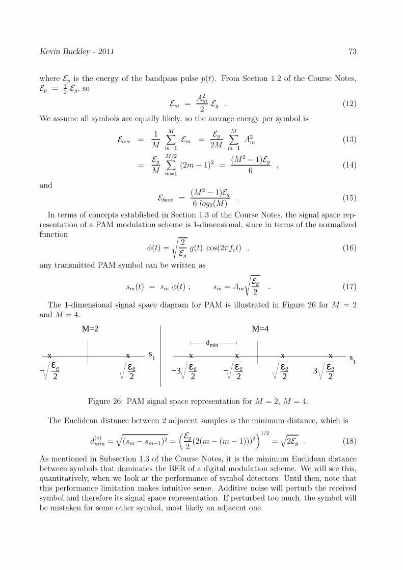
Kevin Buckley - 2011 73
where Ep is the energy of the bandpass pulse p(t). From Section 1.2 of the Course Notes,Ep = 1
2Eg, so
Em =A2
m
2Eg . (12)
We assume all symbols are equally likely, so the average energy per symbol is
Eave =1
M
M∑
m=1
Em =Eg2M
M∑
m=1
A2m (13)
=EgM
M/2∑
m=1
(2m− 1)2 =(M2 − 1)Eg
6, (14)
and
Ebave =(M2 − 1)Eg6 log2(M)
. (15)
In terms of concepts established in Section 1.3 of the Course Notes, the signal space rep-resentation of a PAM modulation scheme is 1-dimensional, since in terms of the normalizedfunction
φ(t) =
√
2
Egg(t) cos(2πfct) , (16)
any transmitted PAM symbol can be written as
sm(t) = sm φ(t) ; sm = Am
√
Eg2
. (17)
The 1-dimensional signal space diagram for PAM is illustrated in Figure 26 for M = 2and M = 4.
ε ε ε ε
mind
ε εs
1
g
2−3 g
2− g
2g
23
s1
M=2 M=4
xx
g
2g
2−
xx x x
Figure 26: PAM signal space representation for M = 2, M = 4.
The Euclidean distance between 2 adjacent samples is the minimum distance, which is
d(e)min =
√
(sm − sm−1)2 =(Eg2(2(m− (m− 1)))2
)1/2
=√
2Eg . (18)
As mentioned in Subsection 1.3 of the Course Notes, it is the minimum Euclidean distancebetween symbols that dominates the BER of a digital modulation scheme. We will see this,quantitatively, when we look at the performance of symbol detectors. Until then, note thatthis performance limitation makes intuitive sense. Additive noise will perturb the receivedsymbol and therefore its signal space representation. If perturbed too much, the symbol willbe mistaken for some other symbol, most likely an adjacent one.

Kevin Buckley - 2011 74
2.2 Phase Modulated Signals - Memoryless & Linear
The general class of phase modulation schemes considered in this Subsection are 2-dimensional,M-symbol, memoryless and linear. The class is also know as phase-shift keying (PSK). TheM symbols are as follows:
sm(t) = g(t) cos (2πfct+ 2π(m− 1)/M) ; 0 ≤ t < T m = 1, 2, · · · ,M . (19)
So, symbols are distinguished by the different phases of the carrier. As with PAM, g(t) is areal-valued pulse shaping waveform.
Eq. 19 can also be written as
sm(t) = Re
g(t) ej2π(m−1)/Mej2πfct
; 0 ≤ t < T m = 1, 2, · · · ,M . (20)
It can be seen form Eq. 20 that the equivalent lowpass representation is
sml(t) = ej2π(m−1)/M g(t) ; 0 ≤ t < T m = 1, 2, · · · ,M . (21)
Figure 27 illustrates s(t) and sl(t) for M = 2 and g(t) equal to a pulse of width T .
s (t)4 s (t−T)3 s (t−3T)12s (t−2T) ls (t)Re ls (t)Im
s (t−T)3l s (t)4l 2l s (t−2T)
t
−1
1j
−j
T2T
3T 4T
....
s (t−3T)1l
t
−1
1
T
....s(t)
4T3T
2T
Figure 27: A PSK signal and its lowpass equivalent for an M = 4 symbol scheme.
So as to derive the signal space representation of PSK, we can, using trigonometric iden-tities, rewrite Eq. 19 as
sm(t) = g(t)
[
cos
(
2π(m− 1)
M
)
cos (2πfct) − sin
(
2π(m− 1)
M
)
sin (2πfct)
]
(22)
= sm1 φ1(t) + sm2 φ2(t) = [φ1(t), φ2(t)] sTm (23)
where the orthonormal basis functions are
φ1(t) =
√
2
Egg(t) cos(2πfct) 0 ≤ t < T (24)
φ2(t) = −√
2
Egg(t) sin(2πfct) 0 ≤ t < T (25)
and the signal space representation (i.e. symbol dependent coefficients of the orthonormalrepresentation) for the mth symbol is
sm = [sm1, sm2] =
√
Eg2cos (2π(m− 1)/M) ,
√
Eg2sin (2π(m− 1)/M)
. (26)
This modulation scheme is 2-dimensional because any symbol can be represented as linearcombinations of φ1(t) and φ2(t). These two basis functions are referred to as the in-phaseand quadrature components, respectively.

Kevin Buckley - 2011 75
Eg
2
Eg
2
Eg
2
Eg
2
s1
s2
xx
x
x
−
−
M=4
s1
Eg
2Eg
2−
xx
M=2
Figure 28: PSK signal space representation for M = 2, M = 4.
For M = 2, we see that
s1 =
√
Eg2
[1 , 0] , s2 =
√
Eg2
[−1 , 0] . (27)
So, φ2(t) is not used, and thus for this case the modulation scheme is only 1-dimensional.Comparing it to PAM with M = 2, we see that the two schemes are identical. For M = 4,we have
s1 =
√
Eg2
[1 , 0] ; s2 =
√
Eg2
[0 , 1] (28)
s3 =
√
Eg2
[−1 , 0] ; s4 =
√
Eg2
[0 , −1] .
Figure 28 shows the signal space diagram for PSK for M = 2 and M = 4. In the M = 4figure note that s1 is the in-phase axis and s2 the quadrature.
PSK is a linear modulation scheme because the transmitted signal s(t) is constructed asa superposition of time shifted sm(t)’s, which are in turn formed as a linear combination ofbasis functions (i.e. Eq. (23)). It is memoryless because an sm or sm(t) depends on only oneblock of an’s, and the superposition of the time shifted sm(t)’s is memoryless.
The energy of a PSK symbol can be determined from any of the representations above.For example, from the signal space representation we can see that, since the symbol energiesare square of the lengths of the symbol vectors, they are all the same, i.e.
Em =Eg2
. (29)
(This can be derived from the signals space coefficient vector noting that cos2(x)+sin2(x) =1). Also, from Eq. 21, the mth lowpass equivalent symbol has energy Eml = Eg. From
Subsection 1.2 of the Course Notes, Em = Eml
2= Eg
2. That all the M symbols have the same
energy should be expected from Eq. 19, since symbols differ only in the phase of the carrier.

Kevin Buckley - 2011 76
For a given M , the symbols are equal-distance from the origin in 2-dimensional space andevenly distributed in phase. The pattern of symbols in the signal space is called the symbol
constellation for the modulation scheme. The minimum Euclidean distance is the distancebetween two adjacent symbols,
d(e)min =
√
Eg(1− cos(2π/M)) . (30)
The transmitted signal s(t) is constructed in a manner similar to PAM, as in Eq. 9, i.e.
s(t) =∑
n
sm(n)(t− nT ) =∑
n
g(t− nT ) cos (2πfct+ 2π(m(n)− 1)/M) (31)
where 2π(m(n) − 1)/M is the phase used at symbol time n to represent the block of kinformation samples from an .
2.3 Quadrature Amplitude Modulation (QAM) - Memoryless &Linear
This is a generalization of the 2-dimensional PSK modulation scheme, where symbols aredistinguished by varying both the amplitude and phase of the carrier (see Eq. 19), orequivalently the coefficients of both the in-phase and quadrature basis functions (see Eq.22).
The M symbols are as follows:
sm(t) = rm g(t) cos (2πfct+ θm) ; 0 ≤ t < T m = 1, 2, · · · ,M , (32)
where rm and θm are the magnitude and phase of the mth symbol. As with PAM and PSK,g(t) is a real-valued pulse shaping waveform.
Eq. 32 can also be written as
sm(t) = Re
rm ejθm g(t) ej2πfct
; 0 ≤ t < T m = 1, 2, · · · ,M . (33)
It can be seen form Eq. 33 that the equivalent lowpass representation is
sml(t) = rm ejθm g(t) ; 0 ≤ t < T m = 1, 2, · · · ,M . (34)
Figure 29 illustrates s(t) and sl(t) for M = 2 and g(t) equal to a pulse of width T .
s (t)4 s (t−T)32s (t−2T) s (t−3T)1 ls (t)Re
2l s (t−2T) 1ls (t−3T)s (t−T)3l s (t)4l
ls (t)Im
t
−1
1
T
....
4T3T
2T
s(t)
3
−3
t
−1
1j
−j
T2T
3T 4T
....
3
−3
−j3
j3
Figure 29: A QAM signal and its lowpass equivalent for an M = 4 symbol scheme.

Kevin Buckley - 2011 77
So as to derive the signal space representation of QAM, we can, using trigonometricidentities, rewrite Eq. 32 as
sm(t) = sm1 φ1(t) + sm2 φ2(t) = [φ1(t), φ2(t)] sTm (35)
where the orthonormal basis functions are the same as for PSK (i.e. see Eqs. 24,25).For the mth symbol, the signal space representation depends on both Vm and θm:
sm = [sm1, sm2] =
√
Eg2
rm cos θm ,
√
Eg2
rm sin θm
=
Am,i
√
Eg2
, Am,q
√
Eg2
, (36)
where Am,i and Am,q are, respectively, the in-phase and quadrature (real and imaginary)components of rm ejθm.
From Eq. 35, the energy of a QAM symbol is the sum of the squares of the symbolcoefficients, which from Eq. 36 is
Em =r2mEg2
. (37)
Unlike PSK, symbols will not have equal energy since amplitude as well as phase is varied.Although the magnitude and phase of QAM symbols can be selected in any way, the two
common schemes are to:
1. select symbols on a circular grid in the signal space; or
2. select symbols on a rectangular grid in the signal space.
In Figure 30 symbol constellations are shown for both of these schemes, for M = 16.As with PSK, this modulation scheme is 2-dimensional, linear and memoryless. The
transmitted signal s(t) is constructed in a manner similar to PAM and PSK. That is,
s(t) =∑
n
sm(n)(t− nT ) =∑
n
rm(n) g(t− nT ) cos(
2πfc(t− nT ) + θm(n)
)
(38)
where rm(n) and θm(n) at symbol time n are selected to represent the block of k informationbits from an .
(b) M−16 QAM on rectangular grid(a) M=16 QAM on circular grid
Figure 30: Signal space representations for two QAM schemes.

Kevin Buckley - 2011 78
2.4 Notes on Multidimensional Modulation Schemes
In Section 1.3 of the Course, where we developed the signal space representation of thesymbols of a digital modulation scheme, symbols sm(t); m = 1, 2, · · · ,M were generallyrepresented using N basis waveforms φj(t); j = 1, 2, · · · , N as
sm(t) =N∑
j=1
smj φj(t) = φ(t) sTm , (39)
where φ(t) = [φ1(t), φ2(t), · · · , φN(t)] represents the basis waveforms and sm is the sig-nal space representation vector for the m − th symbol. Earlier we saw that PAM is a1-dimensional modulation scheme (i.e. N = 1), whereas PSK and QAM are in general2-dimensional.
Here we overview several linear, memoryless higher dimensional digital modulation schemes.In general, we assume that the basis waveforms are linearly independent but not necessarilyorthogonal. This discussion corresponds to Subsection 3.2-4 of the Course Text.
2.4.1 Orthogonal Signal
Orthogonal signaling refers to a modulation scheme with orthogonal symbols. Generally, withorthogonal symbols, we allocate a different orthogonal waveform to each symbol. Assumethe set of basis waveforms φj(t); j = 1, 2, · · · , N are orthonormal. Let E denote the energyof each and every symbol, i.e.
E = < sm(t), sm(t) > =∫ T
0s2m(t) dt ; m = 1, 2, · · · ,M (40)
where T is the symbol (and basis waveform) duration. So that each symbol representsk = log2(M) bits, the energy/ bit is
Eb =E
log2(M). (41)
In terms of Eq. 39 representation, for orthogonal symbols, we simply have
sm(t) =√E φm(t) ; m = 1, 2, · · · ,M . (42)
i.e. N = M (each symbol has its own orthogonal basis waveform). Then, the signal spacevector for the m− th symbols is
sm = [0, 0, · · · , 0 ,√E , 0, · · · , 0] (43)
where the nonzero element is in the m − th position. The Euclidean distance between anytwo symbols in the same, and by the Pythagorean theorem, this common (i.e. minimum)distance is
dmin =√2 E . (44)

Kevin Buckley - 2011 79
2.4.2 Frequency Shift Keying (FSK)
With FSK, each symbol is a sinusoid of a different frequency. Typically, these frequenciesare equi-spaced, so we have that
sm(t) =
√
2ET
cos(2π(fc + k∆f)t) ; 0 ≤ t < T ; m = 1, 2, · · · ,M (45)
= Resml(t) ej2πfct (46)
where ∆f is the frequency spacing, and the lowpass equivalents are then of the form
sml(t) =
√
2ET
ej2πm∆ft . (47)
The modulation index in FSK is defined as fk = ∆f/fc. If ∆f is an integer multiple of12T, then the symbols are orthogonal and FSK is an orthogonal signaling scheme (see Eqs
(3.2-57, 3.2-58), p. 110 of the Course Text).For FSK with M = 2, termed Binary FSK, the values 0 and 1 of a binary sample an are
transmitted by pulses represented as follows:
0 is represented by a√
2ET
cos(2πfc − π∆f)t 0 ≤ t < T , and
1 is represented by a√
2ET
cos(2πfc + π∆f)t 0 ≤ t < T .
One obvious way to generate a binary FSK signal is to switch between two independentoscillators according to whether the data bit is a 0 or 1. Typically, this form of FSK gen-eration results in a waveform that is discontinuous in amplitude or slope at the switchingtimes. Because of these possible discontinuities, FSK can have undesirable Power SpectralDensity (PSD) spread (i.e. it used frequency resources inefficiently). This motivates con-tinuous phase approaches, which employ memory to assure that phase transitions betweensymbols are continuous. As we will see later in this Subsection, continuous phase approachesare nonlinear and have memory.
A minor point: Note that on p. 110 of the Course Text the authors imply a definition oflinearity of a modulation scheme – that a modulation scheme is linear if the sum of any twosymbols is a waveform that is in the same class of symbols, but not necessarily a member thethe set of symbols for that specific modulation scheme (i.e. the sum of two QAM waveformsis a QAM waveform). This is not the same notion of linearity that I have used (i.e. that thetransmitted waveform is constructed as superposition of individual symbols).
2.4.3 Biorthogonal Signaling
In Biorthogonal signaling, M symbols, sm(t); m = 1, 2, · · · ,M , are represented by N = M2
orthonormal basis waveforms, φj(t); j = 1, 2, · · · , M2. Each orthonormal basis waveform
represents two symbols as follows:
s(j+1)/2(t) =√E φj(t) ; s(j+3)/2(t) = −
√E φj(t) ; j = 1, 2, · · · , N . (48)
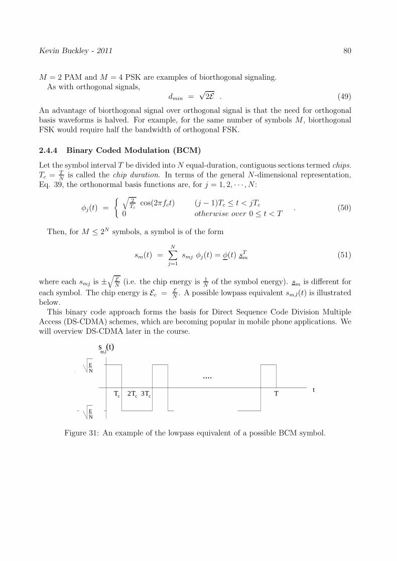
Kevin Buckley - 2011 80
M = 2 PAM and M = 4 PSK are examples of biorthogonal signaling.As with orthogonal signals,
dmin =√2E . (49)
An advantage of biorthogonal signal over orthogonal signal is that the need for orthogonalbasis waveforms is halved. For example, for the same number of symbols M , biorthogonalFSK would require half the bandwidth of orthogonal FSK.
2.4.4 Binary Coded Modulation (BCM)
Let the symbol interval T be divided intoN equal-duration, contiguous sections termed chips.Tc = T
Nis called the chip duration. In terms of the general N -dimensional representation,
Eq. 39, the orthonormal basis functions are, for j = 1, 2, · · · , N :
φj(t) =
√
2Tc
cos(2πfct) (j − 1)Tc ≤ t < jTc
0 otherwise over 0 ≤ t < T. (50)
Then, for M ≤ 2N symbols, a symbol is of the form
sm(t) =N∑
j=1
smj φj(t) = φ(t) sTm (51)
where each smj is ±√
E
N(i.e. the chip energy is 1
Nof the symbol energy). sm is different for
each symbol. The chip energy is Ec = E
N. A possible lowpass equivalent sm,l(t) is illustrated
below.This binary code approach forms the basis for Direct Sequence Code Division Multiple
Access (DS-CDMA) schemes, which are becoming popular in mobile phone applications. Wewill overview DS-CDMA later in the course.
EN
EN
Tc TcTc
s (t)m,l
t
....
2 3 T
Figure 31: An example of the lowpass equivalent of a possible BCM symbol.

Kevin Buckley - 2011 81
2.5 Several Modulation Schemes with Memory
In this Subsection we describe several modulation schemes that use symbol or informationbit memory. There are several reasons to consider using memory. The most importantconsiderations are: 1) receiver simplification; 2) transmitted signal spectral characteristics.We consider three schemes:
• Binary Differential PSK (DPSK);
• Partial Response Signaling (PRS); and
• Continuous-Phase Modulation (CPM).
These illustrate the two considerations listed above, and also facilitate the introduction ofan important structure, the trellis diagram, for representing digital communication systemsthat operate with modulation, error-control or channel memory.
2.5.1 Differential PSK (DPSK)
DPSK is a linear modulation scheme with memory. It is not introduce in the Course Textuntil Chapter 4, on p. 195, where it is presented as an approach to eliminating the needfor carrier synchronization (i.e. knowledge of the carrier sinusoid phase) at the receiver. Weintroduce it here because it is an important and simple example of a modulation schemewith memory. We describe only binary DPSK.
Conceptually, DPSK is derived by combining a general differential encoding scheme withPSK. The encoding scheme, differential non return to zero inverted or NRZI, can haveattractive spectral shaping characteristics for some applications, and results in a simplifiedreceiver. However, compared to standard PSK there is a reduction in performance.
With NRZI, the symbol being transmitted changes only if a ”1” bit is transmitted. If a”0” is being transmitted, then the same symbol previously transmitted is transmitted again.Thus, at the receiver, the detection of a symbol change indicates that a ”1” was transmitted.No change results in a decision that a ”0” was transmitted. For DPSK, a ”1” is indicated bya 180o change in carrier phase. Thus, knowledge of transmitter phase in not required at thereceiver, only an ability to detect phase change is needed. Also, the receiver is not sensitiveto unknown phase shifts implemented by the channel. A transmitted DPSK is illustrated inFigure 32.
Since the current symbol depends on the past symbols, NRZI incorporates memory. Toillustrate this, let an and bn represent, respectively, an original binary sequence and its NRZIcode. These are related as illustrated with the digital system below, where the adder is abinary adder. The memory is introduced by the delayed output feedback.
The NRZI sequence bn is used to select the binary symbol for the M = 2 symbol modu-lation scheme (e.g. bn = 0 −→ s0(t), bn = 1 −→ s1(t)).
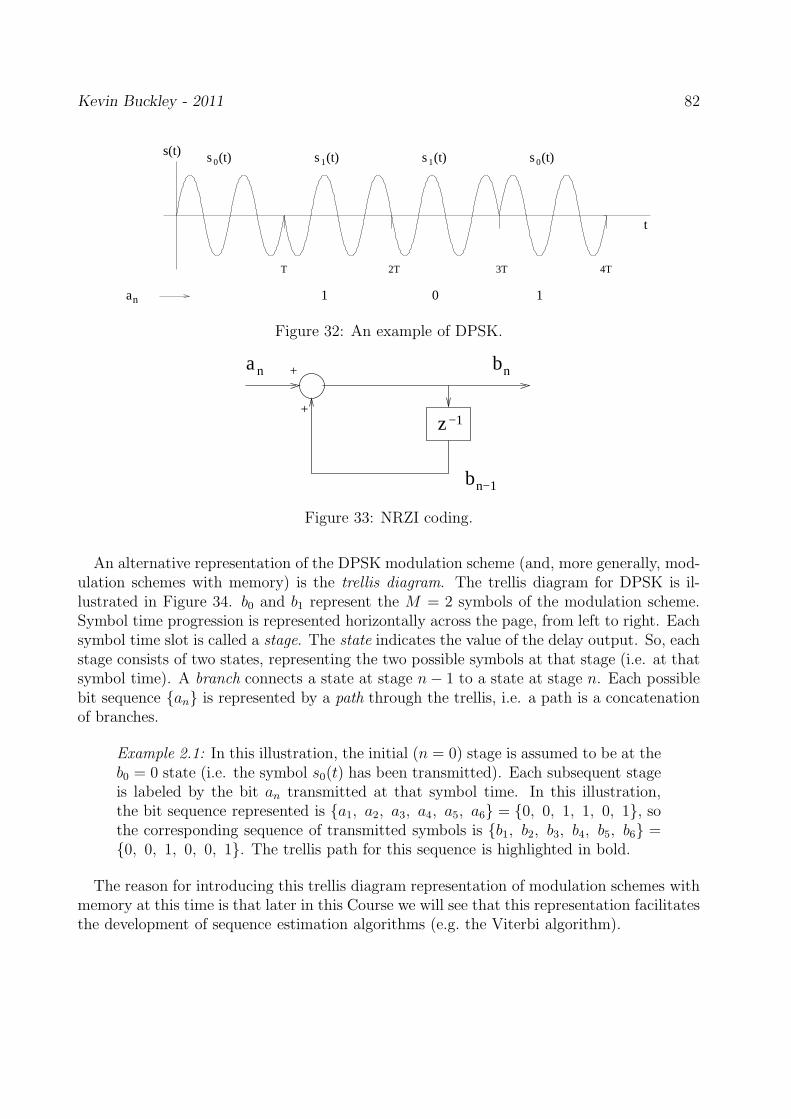
Kevin Buckley - 2011 82
s (t)1 s (t)1 s (t)0s (t)0
an
s(t)
2T 3T 4TT
1 0 1
t
Figure 32: An example of DPSK.
z−1
bnan
bn−1
+
+
Figure 33: NRZI coding.
An alternative representation of the DPSK modulation scheme (and, more generally, mod-ulation schemes with memory) is the trellis diagram. The trellis diagram for DPSK is il-lustrated in Figure 34. b0 and b1 represent the M = 2 symbols of the modulation scheme.Symbol time progression is represented horizontally across the page, from left to right. Eachsymbol time slot is called a stage. The state indicates the value of the delay output. So, eachstage consists of two states, representing the two possible symbols at that stage (i.e. at thatsymbol time). A branch connects a state at stage n− 1 to a state at stage n. Each possiblebit sequence an is represented by a path through the trellis, i.e. a path is a concatenationof branches.
Example 2.1: In this illustration, the initial (n = 0) stage is assumed to be at theb0 = 0 state (i.e. the symbol s0(t) has been transmitted). Each subsequent stageis labeled by the bit an transmitted at that symbol time. In this illustration,the bit sequence represented is a1, a2, a3, a4, a5, a6 = 0, 0, 1, 1, 0, 1, sothe corresponding sequence of transmitted symbols is b1, b2, b3, b4, b5, b6 =0, 0, 1, 0, 0, 1. The trellis path for this sequence is highlighted in bold.
The reason for introducing this trellis diagram representation of modulation schemes withmemory at this time is that later in this Course we will see that this representation facilitatesthe development of sequence estimation algorithms (e.g. the Viterbi algorithm).

Kevin Buckley - 2011 83
n=1 n=2 n=4n=3 n=5 n=6n=0
1a = 0 a = 0 a = 1 a = 1 a = 0 a = 12 3 4 5 6
state 1; b = 1
state 0; b = 0n−1
n−1
Figure 34: Trellis diagram representation of DPSK.
2.5.2 Partial Response Signaling (PRS)
PRS is a general scheme, which has memory and may or may not be linear, depending on themodulation scheme employed. PRS refers to a technique for preprocessing symbols, priorto modulation, which is used to shape the spectrum on the transmission in considerationof frequency response characteristics of the channel. We will see how this spectral shapingis characterized below in Section 2.6. Here we introduce PRS by illustrating the techniqueusing the example explored in Problem 3.14 of the Course Text.
Example 2.2: Consider the following representation of a bit an at binary symboltime n:
In = 2 · an − 1 i.e. an = 1 −→ In = 1 , an = 0 −→ In = −1 . (52)
So, In ∈= ±1. Figure 36 depicts a discrete-time linear, time-invariant systemwhich processes a sequence In to produce a PRS sequence Bn.
nIz−1
+
+
n−1I
B n
Figure 35: PRS example (from Problem 4.21 of the Course Text).
The corresponding trellis diagram is shown in Figure 36.
The path for input sequence In = −1, −1, 1, 1, · · · is highlighted. Thebranches are labeled with the PRS output corresponding to the states that branchconnects. The PRS sequence corresponding to the highlighted path is Bn =0, −2, 0, 2, 0, 0, · · ·.
Again note that we will depend on trellis diagrams later in the Course, to provide a structurefor developing efficient sequence estimation algorithms.

Kevin Buckley - 2011 84
B = 22B = 21
1B = 02B = 0
2B = −2
2B = 0
n=1 n=2 n=4n=3 n=5 n=6n=0
1I = −1 I = −1 I = 1 I = 1 I = −1 I = 1
2
−2
0
0
2 2 2
−2 −2 −2
0 0 0
0 0 0
2 3 4 5 6
state 0; I = 1
state 1; I = −1n−1
n−1
Figure 36: PRS trellis diagram (for Problem 4.21 of the Course Text).
2.5.3 Continuous-Phase Modulation (CPM)
CPM is a nonlinear modulation scheme with memory.In our earlier discussion on FSK, it was noted that the discontinuity in phase in the
transition between symbols can render this approach unattractive. Here we describe analternative which eliminates this problem. We start by developing the Continuous PhaseFSK (CPFSK) modulation scheme and then generalize to CPM.
For FSK signal representation, a common alternative to oscillator switching is to frequencymodulate a single carrier oscillator using the message waveform. With this approach, CPFSKtransmitted waveforms can be represented as
s(t) =
√
2E
Tcos[2πfct + φ(t) + φ0], (53)
where
φ(t) = 4πTfd
∫ t
−∞
d(τ)dτ , (54)
where 1Tis the symbol rate, fd is termed the peak frequency deviation, φ0 is the initial phase,
and d(t) is the information (modulating) signal. For digital communication, let In be thesequence of amplitudes, each representing k bits from an. Then the information signal is
d(t) =∑
n
In g(t− nT ) (55)
where g(t) is a pulse shaping waveform. As used here In, which represents a sequence ofblocks of information bits, is a discrete-time, discrete-valued sequence1. With this approach,even though for digital communications the modulating waveform d(t) may be discontinuousat symbol transitions, the phase function φ(t) is proportional to the integral of d(t) and willbe continuous (as long as there are no impulses in g(t), which there will not be).
Clearly, φ(t) has infinite memory. That is, it is a function of the present and all previousIn which represent the blocks of k an’s. So the CPFSK modulation scheme has memory. Itis also nonlinear since s(t) is not a linear function of the In.
1This notation was introduced earlier, at the beginning of Section 2 of this Course, to introduce the
concepts of memory and states. This notation will be used extensively later in the Course in discussions
of detection, sequence estimation and intersymbol interference channels. For its current use in describing
CPFSK, In is real-valued. As used later for other modulation schemes, it may be complex-valued.

Kevin Buckley - 2011 85
The phase will now be denoted φ(t; I) to indicate that it is a function of the vector I ofinformation bearing amplitudes In. It can be written as
φ(t) = φ(t; I) = 4πTfd
∫ t
−∞
[
∑
n
Ing(τ − nT )
]
dτ . (56)
Define the modulation index as the quantity h = 2Tfd. Assuming for now that g(t) islimited to 0 ≤ t ≤ T and has a total area of 1
2, and denoting q(t) =
∫ t−∞
g(τ)dτ , we havethat
φ(t; I) = 2πh
Inq(t− nT ) +1
2
n−1∑
k=−∞
Ik
; nT ≤ t < (n+ 1)T (57)
= 2πhInq(t− nT ) + θn ; nT ≤ t < (n + 1)T ,
where θn = πh∑n−1
k=−∞Ik. Later in the Course, this final form of φ(t; I) will be used to
derive a computationally efficient optimum receiver structure for CPFSK (more generally,for CPM).
Figure 37 illustrates two pulse shapes commonly used in continuous phase modulationsschemes. As shown, both of these pulses are limited to 0 ≤ t < T . The first is a rectangularpulse, and the second illustrates what is termed, for CPFSK, a “Gaussian” pulse.
g(t)
q(t)
t
g(t)
q(t)
tT
1/2T1/2T
T
T T
Figure 37: Common continuous phase modulation scheme pulse shapes.

Kevin Buckley - 2011 86
A more general class of modulation schemes is defined by generalizing the Eq (57) phaseexpression as follows:
φ(t; I) = 2πn∑
k=−∞
Ik hk q(t− kT ) ; nT ≤ t < (n+ 1)T , (58)
where hk is a modulation index sequence. This generalization is referred to as CPM. CPMis called full-response if the pulse g(t) is limited to 0 ≤ t < T (as it is assumed to be abovestarting with Eq (57)). Note that, in Eq (57), the sum is over all past symbols, since withg(t) restricted to 0 ≤ t < T , at any time t all but the current pulse has been completelyintegrated over. If the pulse has a larger width than T (again note that T is defined such that1Tis the symbol rate), than at any time T more that one pulse will not be fully integrated
over. We call this partial-response CPM. For example, say that the pulse has width betweenT and 2T . Then, Eq (57), generalized for CPM, becomes
φ(t; I) = 2πhnInq(t−nT )+2πhn−1In−1q(t−(n−1)T )+πn−2∑
k=−∞
Ikhk ; nT ≤ t < (n+1)T .
(59)Gaussian Minimum Shift Keying (GMSK) is, generally, partial-response CPM with a “Gaus-sian” pulse shape.
Later in the Course, in discussions on sequence estimation, we will develop the trellisdiagram representation for CPM.
2.6 Spectral Characteristics of Digitally Modulated Signals
This Subsection of the Course Notes corresponds to topics in Subsections 2.7-2 and 3.4-2 ofthe Course Text. Our objective is to characterize the frequency content of digitally modulatedsignals. This is a critically important issue in most digital communications applicationsbecause of the need to efficiently utilize limited channel bandwidth. We will restrict thisdiscussion to linear modulations schemes with and without memory. See Section 3.4 of theCourse Text for spectral characteristics of some other modulation schemes.
Consider a modulation scheme that generates transmitted signal s(t) with lowpass equiv-alent v(t) = sl(t) that can be represented as
v(t) =∑
n
Im(n) g(t− nT ) , (60)
where g(t) is a baseband pulse shape and In is a discrete-time, discrete-valued, generallycomplex-valued sequence. For example, PAM, PSK and QAM can be represented this way,where
Im(n) = Am(n) (PAM : Lect4 Notes, Eq(8)) (61)
Im(n) = ej2π(m(n)−1)/M (PSK : Lect4 Notes, Eq(21)) (62)
Im(n) = rm(n) ejθm(n) (QAM : Lect4 Notes, Eq(34)) . (63)
The transmitted signal s(t) is a random process since the In sequence is random. Wefirst show that v(t) (and therefore s(t)) is not wide-sense stationary. This is because of the

Kevin Buckley - 2011 87
within-symbol structure (i.e. the g(t) structure). However, if In is wide-sense stationary,which we assume it is, then v(t) (and therefore s(t)) is cyclostationary, and we can identify2nd order statistical characterizations (i.e. correlation and frequency spectrum).
We know, from our previous discussion of equivalent lowpass signals, that the spectralcharacteristics of s(t) can be determined from those of v(t), e.g. for wise-sense stationarys(t) the power density spectrum relationship is
SS(f) =1
4[SV (f − fc) + SV (−f − fc)] . (64)
So, we proceed to characterize the frequency characteristics of v(t) and then deduce thoseof s(t).
Let mI be the mean of wide-sense stationary random sequence Im(n) = In. Then
Ev(t) = E∑
n
In g(t− nT ) = mI
∞∑
n=−∞
g(t− nT ) . (65)
So, the mean of v(t) (and thus s(t)) is periodic with period T , and Ev(t) = 0 if mI = 0.By definition, a cyclostationary signal has a mean and autocorrelation function that are
periodic in t with some period T . The autocorrelation function of the equivalent lowpasssignal v(t) is defined as
RV (t, t− τ) = Ev(t) v∗(t− τ) . (66)
Plugging in v(t) =∑
∞
n=−∞In g(t− nT ), and letting
RI [l] = EIn I∗n−l (67)
denote the discrete-time autocorrelation function of wide-sense stationary In, we get anexpression for RV (t, t− τ). It can be shown that this expression for RV (t, t− τ) is periodicwith period T .
So v(t) is cyclostationary. For such a signal, it is standard practice and it makes sense todefine a time averaged autocorrelation function as
RV (τ) =1
T
∫ T
0RV (t, t− τ) dt . (68)
Evaluating Eq (68) to derive a corresponding spectral measure, first note that
RV (τ) =1
T
∫ T
0E
∞∑
l=−∞
Il g(t− lT ) ·∞∑
m=−∞
Im g((t− τ)−mT ) dt (69)
=1
T
∞∑
l=−∞
EIl∞∑
m=−∞
Im
∫ T
0g(t− lT ) g((t− τ)−mT ) dt . (70)
Substituting t1 = t− lT , we have
RV (τ) =1
T
∞∑
l=−∞
EIl∞∑
m=−∞
Im
∫ T−lT
−lTg(t1) g(t1 − τ − (m− l)T ) dt1 . (71)

Kevin Buckley - 2011 88
Substituting n = m− l, we have
RV (τ) =1
T
∞∑
l=−∞
EIl∞∑
n=−∞
Il−n
∫ T−lT
−lTg(t1) g(t1 − τ + nT ) dt1 (72)
=1
T
∞∑
n=−∞
∞∑
l=−∞
EIl Il−n∫ T−lT
−lTg(t1) g(t1 − τ + nT ) dt1 (73)
=1
T
∞∑
n=−∞
RI [n]∞∑
l=−∞
∫ T−lT
−lTg(t1) g(t1 − τ + nT ) dt1 (74)
=1
T
∞∑
n=−∞
RI [n]∫
∞
−∞
g(t1) g(t1 − τ + nT ) dt1 (75)
=1
T
∞∑
n=−∞
RI [n] Rc(τ − nT ) , (76)
whereRG(τ) =
∫
∞
−∞
g(t) g(t− τ) dt . (77)
Defining the DT function RcI(τ) from the DT function RI [n] as
RcI(τ) =
1
T
∞∑
n=−∞
RI [n] δ(τ − nT ) , (78)
it is straight forward to show that Eq (76) can be expressed as the CT convolution
RV (τ) = RcI(τ) ∗RG(τ) . (79)
We can use this form of the time averaged autocorrelation function of cyclostationary v(t)to define and evaluate an average PSD.
Define SV (f), the continuous-time Fourier transform (CTFT) of RV (τ), as the average
PSD. Then, from the convolution property of Fourier transforms,
SV (f) = ScI(f) SG(f) (80)
where the two terms on the right are the CTFT’s of the respective autocorrelation functions.ScI(f) is periodic with period 1
Tsince Rc
I(τ) consists of impulses at integer multiples of T . Youmay recall for studying sampling theory that Sc
I(f) =1TSI(f) where SI(f) = DTFTRI [l],
i.e.
SI(f) =∞∑
l=−∞
RI [l] e−j2πfT l (81)
where, because of the 2πfT l argument of the exponential in the DTFT, f is in cycles/second(as opposed to cycles/sample when 2πfl is used as the argument). Note that SI(f) is thenperiodic with period 1
T.
From the definition of RG(τ) in Eq (77) and properties of the CTFT we have thatSG(f) = |G(f)|2, the magnitude-squared of the CTFT of g(t). Thus, the average PSDcan be expressed as
SV (f) =1
T|G(f)|2 SI(f) . (82)
Kevin Buckley - 2011 89
Note that |G(f)|2, the magnitude-squared of the CTFT of the symbol pulse shape g(t), isoften used to represent the frequency content of v(t). This is the energy spectrum of a singletransmitted symbol. Eq (82), the average PSD of the lowpass equivalent cyclostationarytransmitted communication signal, is more accurate and useful because it incorporates theeffect of correlation across the symbol sequence In. One important consequence of thisis that we can consider designing the correlation function of In so as to control spectralcharacteristics of v(t) (and this s(t)).
Example 2.3: Consider an In which is uncorrelated sample-to-sample, so that
RI [l] =
σ2I +m2
I l = 0m2
I l 6= 0 .(83)
Then the PSD of In is
SI(f) = σ2I +m2
I
∞∑
l=−∞
e−j2πflT = σ2I +
m2I
T
∞∑
l=−∞
δ(f − l
T) . (84)
Then, from Eq. 82,
SV (f) =σ2I
T|G(f)|2 +
m2I
T 2
∞∑
l=−∞
∣
∣
∣
∣
∣
G(l
T)
∣
∣
∣
∣
∣
2
δ(f − l
T) . (85)
Form the derivation above and Example 2.3, we observe the following:
1. We can use the pulse shaping waveform g(t) to control the spectrum SV(f) and there-fore of
SS(f) =1
4[SV (f − fc) + SV (−f − fc)] . (86)
2. We can use correlation in In, i.e. memory in the generation of the In sequence, tocontrol the spectrum of s(t).
3. We want In to be zero-mean so there are no impulses in SI(f) at integer multiples of1T.
so, if In is zero-mean, then the bandwidth of s(t) is the two-sided bandwidth of g(t).Figure 38 illustrates |G(f)|2 for several common pulse shapes. Notice that the zero-
crossing bandwidths of all pulses are proportional to 1T. Compared to the rectangular pulse,
the raised-cosine pulse has twice the zero-crossing bandwidth and lower ”side lobe” levels.The sinc pulse is an ideal bandlimited pulse shape.
Note that for these linear modulation schemes the bandwidth of s(t) is not effected by thenumber of symbol levels.
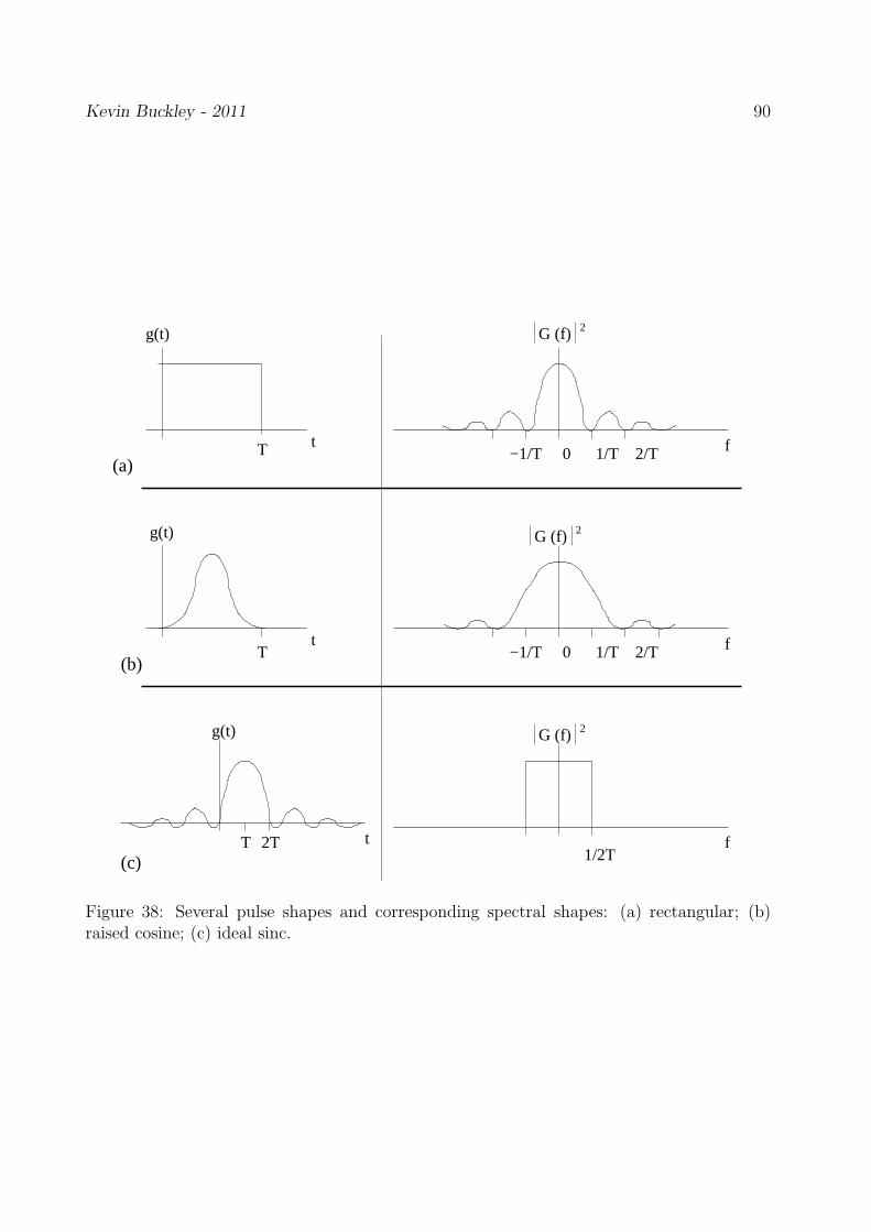
Kevin Buckley - 2011 90
g(t)
T
G (f) 2
G (f) 2
G (f) 2
f1/2T
g(t)
T
−1/T 0 1/T 2/T
t
t f
f−1/T 0 1/T 2/T
(a)
(b)
(c)tT 2T
g(t)
Figure 38: Several pulse shapes and corresponding spectral shapes: (a) rectangular; (b)raised cosine; (c) ideal sinc.


Kevin Buckley - 2011 89
ECE8700Communication Systems Engineering
Villanova UniversityECE Department
Prof. Kevin M. Buckley
Lectures 5,6
0
T( . ) dt
0
T( . ) dt
r
Maximum Likelihood (ML)
Detector
(i.e. nearestneighbor, minimumdistance)
.....
r(t)
T
.....
1
N
(t)
(t)
φ
φ

Kevin Buckley - 2011 90
Contents
3 Symbol Detection 913.1 Correlation Receiver & Matched Filter for Symbol Detection . . . . . . . . . 95
3.1.1 Correlation Receiver . . . . . . . . . . . . . . . . . . . . . . . . . . . 953.1.2 Matched Filter . . . . . . . . . . . . . . . . . . . . . . . . . . . . . . 1033.1.3 A Note on Coherent and Synchronous Reception . . . . . . . . . . . . 1033.1.4 Nearest Neighbor Detection . . . . . . . . . . . . . . . . . . . . . . . 104
3.2 Optimum Symbol Detector . . . . . . . . . . . . . . . . . . . . . . . . . . . . 1063.2.1 Maximum Likelihood (ML) Detector . . . . . . . . . . . . . . . . . . 1063.2.2 Maximum A Posterior (MAP) Detector . . . . . . . . . . . . . . . . . 108
3.3 Performance of Linear, Memoryless Modulation Schemes . . . . . . . . . . . 1113.3.1 Binary PSK . . . . . . . . . . . . . . . . . . . . . . . . . . . . . . . . 1123.3.2 Binary Orthogonal Modulation . . . . . . . . . . . . . . . . . . . . . 1133.3.3 M-ary Orthogonal Modulation . . . . . . . . . . . . . . . . . . . . . . 1153.3.4 M-ary PSK . . . . . . . . . . . . . . . . . . . . . . . . . . . . . . . . 1163.3.5 M-ary PAM . . . . . . . . . . . . . . . . . . . . . . . . . . . . . . . . 1163.3.6 M-ary QAM . . . . . . . . . . . . . . . . . . . . . . . . . . . . . . . . 1173.3.7 M-ary Orthogonal FSK Modulation . . . . . . . . . . . . . . . . . . . 1173.3.8 Examples of Performance Analysis . . . . . . . . . . . . . . . . . . . 1183.3.9 A Performance/SNR/Bandwidth Comparison of Modulation Schemes 119
List of Figures
39 Digital communication channel block diagram under consideration in this Sec-tion. . . . . . . . . . . . . . . . . . . . . . . . . . . . . . . . . . . . . . . . . 94
40 Digital communication receiver – receiver filter/demodulator and detector. . 9541 Bandpass and equivalent lowpass implementations of a correlator receiver. . 9642 A correlator receiver for an ongoing sequence of transmitted symbols. . . . . 10243 Matched filter implementation of the k − th basis function correlation receiver.10344 The ML detector. . . . . . . . . . . . . . . . . . . . . . . . . . . . . . . . . . 10845 (a) the 8-PSK constellation; and (b) a Gray code bit mapping. . . . . . . . . 11146 The receiver statistic (r = x) conditional PDF’s. For ML, T = 0. . . . . . . . 11347 Signal space representation for binary orthogonal modulation. . . . . . . . . 11448 Performance curves for several modulation schemes. . . . . . . . . . . . . . . 11849 Comparison of SNR and bandwidth characteristics of several modulation
schemes at SEP = 10−5. . . . . . . . . . . . . . . . . . . . . . . . . . . . . . 120
Kevin Buckley - 2011 91
Part 2: Symbol Detection and Sequence Estimation
In Part 1 of this Course we established a variety of representations of communicationssymbols and noise. We used these to describe the signals involved in several importantdigital modulation schemes. In this Part of the Course we investigate digital modulationscheme receivers of for an AWGN channel, i.e. when symbols are received in AWGN withno channel-induced symbol distortion. This is the topic of Chapters 4 and 5 of the CourseText. In Part 3 of this Course we will discuss receivers for the AWGN plus symbol distortioncase.
First, in Section 3, we discuss symbol detection. That is, we address the problem of detect-ing a single symbol (i.e. deciding which symbol was transmitted). This is the appropriatereceiver strategy for a AWGN channel when there is no correlation in the symbol sequenceor memory in the modulation scheme. We will cover selected topics from Section 4.1 through4.4 of the Course Text.
Next, in Section 4, we will consider sequence estimation. With this receiver strategy, awhole sequence of symbols is estimated at once, processing the received signal over the entireduration of the sequence. For an AWGN channel, this more complex receiver objective isnecessary for optimum symbol reception when either the symbol sequence is correlated or themodulation scheme is not memoryless. This discussion corresponds to material in Sections4.8 and 4.9 of the Course Text.
In the last Section of this Part of the Course, we will overview topics related to thereception of symbols through a AWGN channel when there is uncertainty at the receiverconcerning the carrier phase on symbol timing. This corresponds to topics in Section 4.5and Chapter 5 on the Course Text.
3 Symbol Detection
In this Section of the Course we consider symbol reception. Topics correspond to Sections4.1 through 4.4 of the Course Text. We assume that each symbol sent is received withoutdistortion (i.e. with the same shape, although in general delayed and attenuated) in additivewhite Gaussian noise (AWGN). Additionally, we assume that there is no memory in thesymbol generation process. That is, the symbol sequence is uncorrelated, and the modulationscheme is memoryless. So, for example, this discussion is relevant to FSK and to QAM and itsspecial cases PSK and PAM. It is not appropriate (as an optimum demodulation approach)for DPSK and modulation schemes using PRS. Under these assumptions, the objective ofthe receiver is to optimally process each noisy received symbol to make a decision as towhich symbol was sent. We will see that, under the assumptions stated above, the optimumreceiver for a memoryless modulation scheme is fairly simple. Later we will see that theoptimum receiver for a system with memory can be substantially more involved.

Kevin Buckley - 2011 92
Review of Signal Representations
1. Symbols (known energy waveforms): Let sm(t); m = 1, 2, · · · ,M be the M symbolsof a modulation scheme. These symbols have frequency content as quantified by theirCTFTs
sm(t)CTFT⇐⇒ Sm(f) =
∫ ∞
−∞sm(t) e
−j2πft dt . (1)
For example, note that the CTFT of any QAM symbol sm(t) = rm g(t) cos(2πfct+θm)is
Sm(f) =rm ejθm
2G(f − fc) +
rm e−jθm
2G(f + fc) , (2)
where G(f) is the CTFT of the pulse shape g(t). So, for QAM, all symbols havethe same spectral shape (i.e. G(f) modulated to ±fc). The energy of a symbol isEm =
∫ T0 s2m(t) dt were 0 ≤ t < T is its assumed temporal extent.
2. Signal Space Representation of Symbols: For M symbols, sm(t); m = 1, 2, · · · ,M , andan N -dimensional linear modulation scheme,
sm(t) =N∑
k=1
smk φk(t) = φ(t) sm m = 1, 2, · · · ,M , (3)
where the φk(t); k = 1, 2, · · · , N are the orthonormal basis functions for the symbols.The sm, which are N -dimensional column vectors, are the signal space representationsof the symbol waveforms. In terms of its signal space representation, the energy of asymbol is
Em =N∑
k=1
|smk|2 = sHm sm . (4)
For memoryless linear modulation schemes, the signal space representation of symbolswill lead directly to simple optimum symbol detection algorithms.
3. The Inner Product: Let the symbol waveforms be time-limited to 0 ≤ t < T . Theφk(t) are therefore also limited in time to this range. The coefficients of the signalspace representation of a symbol waveform are computed as the inner products
smk = < sm(t), φk(t) > =∫ T
0sm(t) φ
∗k(t) dt . (5)
Let s and r be two vectors in the signal space. Their inner product is
< s, r > = rH s =N∑
k=1
sk r∗k . (6)
In terms of this inner product, the energy of a symbol sm(t) is
Em = < sm(t), sm(t) > = < sm, sm > . (7)
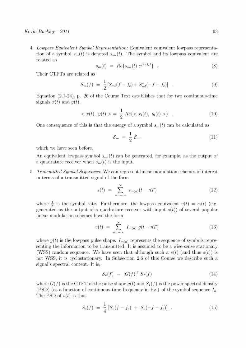
Kevin Buckley - 2011 93
4. Lowpass Equivalent Symbol Representation: Equivalent equivalent lowpass representa-tion of a symbol sm(t) is denoted sml(t). The symbol and its lowpass equivalent arerelated as
sm(t) = Resml(t) ej2πfct . (8)
Their CTFTs are related as
Sm(f) =1
2[Sml(f − fc) + S∗
ml(−f − fc)] . (9)
Equation (2.1-24), p. 26 of the Course Text establishes that for two continuous-timesignals x(t) and y(t),
< x(t), y(t) > =1
2Re< xl(t), yl(t) > . (10)
One consequence of this is that the energy of a symbol sm(t) can be calculated as
Em =1
2Eml (11)
which we have seen before.
An equivalent lowpass symbol sml(t) can be generated, for example, as the output ofa quadrature receiver when sm(t) is the input.
5. Transmitted Symbol Sequences: We can represent linear modulation schemes of interestin terms of a transmitted signal of the form
s(t) =∞∑
n=−∞sm(n)(t− nT ) (12)
where 1T
is the symbol rate. Furthermore, the lowpass equivalent v(t) = sl(t) (e.g.generated as the output of a quadrature receiver with input s(t)) of several popularlinear modulation schemes have the form
v(t) =∞∑
n=−∞Im(n) g(t− nT ) (13)
where g(t) is the lowpass pulse shape. Im(n) represents the sequence of symbols repre-senting the information to be transmitted. It is assumed to be a wise-sense stationary(WSS) random sequence. We have seen that although such a v(t) (and thus s(t)) isnot WSS, it is cyclostationary. In Subsection 2.6 of this Course we describe such asignal’s spectral content. It is,
Sv(f) = |G(f)|2 SI(f) (14)
where G(f) is the CTFT of the pulse shape g(t) and SI(f) is the power spectral density(PSD) (as a function of continuous-time frequency in Hz.) of the symbol sequence In.The PSD of s(t) is thus
Ss(f) =1
4[Sv(f − fc) + Sv(−f − fc)] . (15)
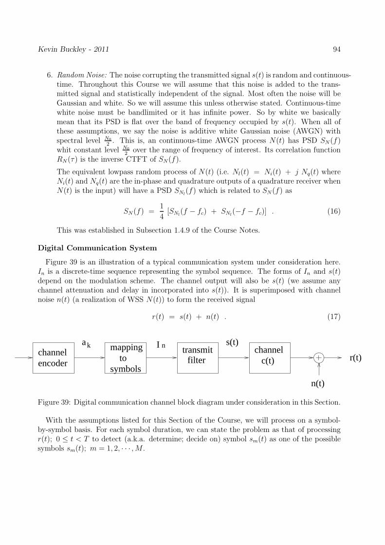
Kevin Buckley - 2011 94
6. Random Noise: The noise corrupting the transmitted signal s(t) is random and continuous-time. Throughout this Course we will assume that this noise is added to the trans-mitted signal and statistically independent of the signal. Most often the noise will beGaussian and white. So we will assume this unless otherwise stated. Continuous-timewhite noise must be bandlimited or it has infinite power. So by white we basicallymean that its PSD is flat over the band of frequency occupied by s(t). When all ofthese assumptions, we say the noise is additive white Gaussian noise (AWGN) withspectral level N0
2. This is, an continuous-time AWGN process N(t) has PSD SN(f)
whit constant level N0
2over the range of frequency of interest. Its correlation function
RN(τ) is the inverse CTFT of SN(f).
The equivalent lowpass random process of N(t) (i.e. Nl(t) = Ni(t) + j Nq(t) whereNi(t) and Nq(t) are the in-phase and quadrature outputs of a quadrature receiver whenN(t) is the input) will have a PSD SNl
(f) which is related to SN(f) as
SN (f) =1
4[SNl
(f − fc) + SNl(−f − fc)] . (16)
This was established in Subsection 1.4.9 of the Course Notes.
Digital Communication System
Figure 39 is an illustration of a typical communication system under consideration here.In is a discrete-time sequence representing the symbol sequence. The forms of In and s(t)depend on the modulation scheme. The channel output will also be s(t) (we assume anychannel attenuation and delay in incorporated into s(t)). It is superimposed with channelnoise n(t) (a realization of WSS N(t)) to form the received signal
r(t) = s(t) + n(t) . (17)
channelencoder
mapping tosymbols
transmitfilter
channel c(t)
ak I n s(t)
n(t)
r(t)
Figure 39: Digital communication channel block diagram under consideration in this Section.
With the assumptions listed for this Section of the Course, we will process on a symbol-by-symbol basis. For each symbol duration, we can state the problem as that of processingr(t); 0 ≤ t < T to detect (a.k.a. determine; decide on) symbol sm(t) as one of the possiblesymbols sm(t); m = 1, 2, · · · ,M .

Kevin Buckley - 2011 95
3.1 Correlation Receiver & Matched Filter for Symbol Detection
Consider a set of symbols sm(t); m = 1, 2, · · · ,M ; 0 ≤ t < T , with sm(n)(t) received atsymbol time n in AWGN. Given the received signal
r(t) = sm(n)(t) + n(t) ; 0 ≤ t < T (18)
the symbol detection objective is to decide which of the M symbols was transmitted.The diagram in Figure 40 depicts the problem and the general form of the receiver. The
receiver front-end demodulates the received signal and filters it prior to sampling and detec-tion. In this Section we describe and justify several common receiver front-ends. Then, inSection 3.2, we describe the detection process.
r
s (t)m(n)
I n
n(t)
r(t)
T
receiverfront−end
decision device(e.g. threshold detector)
Figure 40: Digital communication receiver – receiver filter/demodulator and detector.
3.1.1 Correlation Receiver
This receiver structure correlates the received signal r(t); 0 ≤ t < T with each of themodulation scheme basis functions, φk(t); k = 1, 2, · · · , N , of the given modulation scheme.This correlation is the inner product, so the correlation receiver forms
r = [r1, r2, · · · , rN ]T (19)
where
rk = < r(t), φk(t) > =∫ T
0r(t) φk(t) dt k = 1, 2, · · · , N (20)
=1
2Re< rl(t), φkl(t) > =
∫ T
0rl(t) φ
∗kl(t) dt (21)
where rl(t) is the lowpass equivalent (i.e. quadrature receiver output) of r(t) and the φkl(t)are the lowpass equivalent basis functions. Note that for an N = 1 dimensional modulationscheme, r(t) is simply correlated with the symbol shape to generate a scalar r. In general ris an N -dimensional vector. It is the representation of r(t); 0 ≤ t < T in the signal space forthe modulation scheme. Also note that exact knowledge of the φk(t) at the receiver impliesphase synchronization.
As we will see later, optimum detection based on the received data r(t); 0 ≤ t < T canbe accomplished by processing the output vector. That is, we will r is a sufficient statisticof this detection problem. This is a compelling justification for using a correlation receiver.

Kevin Buckley - 2011 96
Figures 41(a,b) show, respectively, the bandpass and equivalent lowpass implementations.In the bandpass implementation illustration, note that the multiplication of r(t) by the φk(t)represents the demodulation process, since the φk(t) are bandpass functions (typically cosineswith an envelope shaped by a pulse shape g(t)). The integrator is effectively a lowpass filter.The integrator output is sampled when the symbol fills the integrator. For the lowpassequivalent implementation illustration, note the demodulation has already taken place.
r 1
r N
lr (t)
r
0
T( . ) dt
21
0
T( . ) dt
21 Re
Re
1,l
(b)
.....
.....
N,l
(t)
(t)
φ
φ
*
*
r
0
T( . ) dt 1r
0
T( . ) dt
r N
.....
.....
r(t)
(t)
(t)
φ
φ
1
N
(a)
Figure 41: Bandpass and equivalent lowpass implementations of a correlator receiver.
So, why correlate r(t) with the fk(t)? As mentioned earlier, we will formally addressthis later in the Course by showing the the optimum detection problem starting with datar(t); 0 ≤ t < T reduces to a problem of processing r (i.e. r is a sufficient statistic for thedetection problem). For now, consider correlating each sm(t) with r(t) (perhaps so as todecide which sm(t) is most correlated with r(t)). We have
∫ T
0r(t) sm(t) dt =
∫ T
0r(t)
N∑
k=1
smkφk(t) dt (22)
=N∑
k=1
smk
∫ T
0r(t) φk(t) dt
=N∑
k=1
smk rk = sTm r .
This establishes that instead of correlating r(t) which each sm(t) we can correlate r(t) witheach φk(t) instead. This is advantageous whenever N < M , which will be the case forexample in PAM, PSK and QAM with large M .
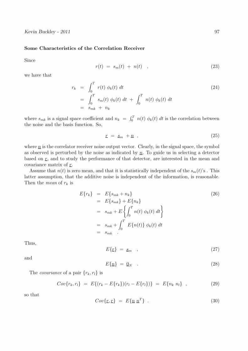
Kevin Buckley - 2011 97
Some Characteristics of the Correlation Receiver
Sincer(t) = sm(t) + n(t) , (23)
we have that
rk =∫ T
0r(t) φk(t) dt (24)
=∫ T
0sm(t) φk(t) dt +
∫ T
0n(t) φk(t) dt
= smk + nk
where smk is a signal space coefficient and nk =∫ T0 n(t) φk(t) dt is the correlation between
the noise and the basis function. So,
r = sm + n , (25)
where n is the correlator receiver noise output vector. Clearly, in the signal space, the symbolas observed is perturbed by the noise as indicated by n. To guide us in selecting a detectorbased on r, and to study the performance of that detector, are interested in the mean andcovariance matrix of r.
Assume that n(t) is zero mean, and that it is statistically independent of the sm(t)’s . Thislatter assumption, that the additive noise is independent of the information, is reasonable.Then the mean of rk is
Erk = Esmk + nk (26)
= Esmk+ Enk
= smk + E
∫ T
0n(t) φk(t) dt
= smk +∫ T
0En(t) φk(t) dt
= smk .
Thus,Er = sm , (27)
andEn = 0N . (28)
The covariance of a pair rk, rl is
Covrk, rl = E(rk − Erk)(rl − Erl) = Enk nl , (29)
so thatCovr, r = En nT . (30)

Kevin Buckley - 2011 98
We have that
Covnk, nl = E
∫ T
0n(t) φk(t) dt ·
∫ T
0n(τ) φl(τ) dτ
(31)
=∫ T
0
∫ T
0En(t) n(τ)φk(t) φl(τ) dt dτ
=N0
2
∫ T
0
∫ T
0δ(t− τ) φk(t)φl(τ) dt dτ =
N0
2
∫ T
0φk(τ)φl(τ) dτ
=N0
2δ(k − l) = σ2
n δ(k − l) .
In going from line 2 to 3 in Eq. 31 above, we make use of the fact that
Rnn(τ) =∫ ∞
−∞SN (f) e
j2πfT df =N0
2δ(τ) , (32)
since the noise is white (i.e. uncorrelated).Thus, given that r(t) = sm(t) + n(t), the correlator output vector has covariance matrix
E(r − sm)(r − sm)T = M =
N0
2IN = σ2
n IN , (33)
where IN is the N ×N identity matrix.Since the input to each correlator is assumed to be Gaussian process, and since the corre-
lator is a linear operator (i.e. a weighted average of the Gaussian input), correlator outputsrk; k = 1, 2, · · · , N are Gaussian. Thus, for a given symbol sm, since r has mean sm andcovariance matrix M , its joint PDF, “conditioned” on sm, is
p(r/sm) =1
(2π)N/2(detM)1/2e−(r−sm)TM−1(r−sm)/2 (34)
=1
(2π)N/2(N0/2)N/2e−|r−sm|2/2(N0/2)
=N∏
k=1
p(rk/smk) ; p(rk/smk) =1√πN0
e−(rk−smk)2/N0 .
This joint PDF of r will be used in the design of optimum detectors. Before we pursue this,let’s look at a couple of examples where r is used within a simple detection scheme based onthe nearest-neighbor in the signal space.

Kevin Buckley - 2011 99
Example 3.1: Two symbol (M=2) PSK

Kevin Buckley - 2011 100
Example 3.2: Four symbol (M=4) PSK (start with Prob. 4.15 of the Course Text)

Kevin Buckley - 2011 101
OK, so in addressing the question “why correlate r(t) with the φk(t)?” we established thefact that, with the vector r of correlations between r(t) and the φk(t), we compute the innerproducts
∫ T
0r(t) sm(t) dt ; m = 1, 2, · · ·M (35)
in an efficient manner when M > N . In zero-mean AWGN with spectral level N0
2, r will have
mean sm (the signal space representation of the transmitted symbol) and covariance matrixM r = σ2
nI where σ2n = N0
2. r has an easily identified Gaussian joint PDF. With Examples
3.1 & 3.2 we see that probabilities of symbol decision error can thus be easily determined,and we can define symbol decision rules in terms of threshold on r.
Several questions remain to be answered:
1. Why base symbol detection on the couple of values in r instead of basing it on r(t); 0 ≤t < T directly? Don’t we lose information or performance by using “just” r?
2. Starting with r(t); 0 ≤ t < T , what is the best detector? Does the optimum detectorreduce to processing r?
3. How do we set thresholds that are optimum with respect of symbol decision errors?
Let’s address the first question first. We will then address question three in Section 3.2. Alittle later in the Course we will address the second question.
We can not reconstruct r(t) from r, so clearly we lose something in going from r(t) to r.But what is it that we lose, and is it anything useful? Consider the following decompositionof r(t):
r(t) = r1(t) + r2(t) , (36)
wherer1(t) = φ(t) r ; 0 ≤ t < T (37)
is the projection of r(t) onto the span of φ(t), and r2(t) is what is left over. r1(t) is therank N approximation of r(t) given the basis functions φk(t); k = 1, 2, · · · , N which form abasis for the sm(t);m = 1, 2, · · · ,M . If r(t) = sm(t), then r1(t) = sm(t). That is, there is noloss of signal – r contains all the information of the symbols. Also, r2(t) contains no symbolcomponent.

Kevin Buckley - 2011 102
Let n1(t) =∑N
k=0 nkφk(t) denote the part of n(t) in the span of the φk(t) and letn2(t) = r2(t) be what is left over. Then
r(t) = sm(t) + n(t) (38)
= sm(t) + n1(t) + n2(t) .
Does n2(t) (i.e. r2(t)) provide us with any information about the noise and/or signal in rwhich is useful? We have that
En2(t) rk = En2(t) smk + En2(t) nk = En2(t) nk (39)
= E
n(t)−N∑
j=0
njφj(t)
nk
= E n(t) nk − E
N∑
j=0
nj nk φj(t)
=∫ T
0En(t) n(τ)φk(τ) dτ −
N∑
j=0
Enj nk φj(t)
=1
2N0 φk(t)−
1
2N0 φk(t) = 0 .
So, r2(t) and the rk are uncorrelated, and since they are also Gaussian, they are statisticallyindependent. This suggests that r2(t) is not useful. Later we will show that, in terms ofsymbol detection, this means that r is a sufficient statistic of r(t). That is, an optimumdetector based on r(t) needs only r.
Consider a transmitted signal composed of a superposition of nonoverlapping symbols,received in additive noise:
r(t) =∑
n
sm(n)(t− nT ) + n(t) . (40)
Figure 42 shows an implementation of the correlator for a ongoing sequence of symbols.φk(t) =
∑
n φk(t−nT ) is the periodic extension of φk(t). The symbols and φk(t) are assumedsynchronized. The integrator integrates over the past T seconds, and the integrator outputis sampled at t = nT ;n = · · · , 0, 1, 2, · · · to form the observation vector sequence rn.
r
(n−1)T
nT( . ) dt
(n−1)T
nT( . ) dt
.....
.....
r(t)
nT
r
r
1,n
N,n
n
1
N(t)
(t)φ
φ
~
~
Figure 42: A correlator receiver for an ongoing sequence of transmitted symbols.

Kevin Buckley - 2011 103
3.1.2 Matched Filter
Consider the linear filter operating on the received signal r(t) shown in Figure 43.
h (t)k
linear filterr(t)
T
Figure 43: Matched filter implementation of the k − th basis function correlation receiver.
Let the filter impulse response be
hk(t) =
φk(T − t) 0 ≤ t ≤ T0 otherwise
, (41)
the k − th basis function for the modulation scheme, folded and shifted so as to be causal.We say that the filter is matched to the basis function φk(t). In general, a matched filtermaximizes the output SNR. In this case it maximizes the SNR for a signal of shape φk(t) inadditive white noise.
The matched filter output is
yk(t) = r(t) ∗ hk(t) =∫ ∞
−∞r(τ) hk(t− τ) dτ (42)
=∫ t
t−Tr(τ) φk(T − t + τ) dτ ; ,
and the output of the sampler is
yk(nT ) =∫ nT
(n−1)Tr(τ) φk(T − nT + τ) dτ (43)
=∫ nT
(n−1)Tr(τ) φk(τ) dτ ,
where as before, φk(t) is the periodic extension of φk(t). Referring back to Subsection 3.1.1,we see that the matched filter implements the correlator receiver.
3.1.3 A Note on Coherent and Synchronous Reception
Kevin Buckley - 2011 104
3.1.4 Nearest Neighbor Detection
Given the N -dimensional sampled output of a matched filter or correlator receiver,
r = sm + n (44)
(i.e. the observation vector), the nearest neighbor symbol detection rule is simply to selectfrom among the symbol signal space vectors sm; m = 1, 2, · · · ,M the one which is closest tothe observation. That is, solve the problem
minsm
||r − sm||2 . (45)
Nearest neighbor detection is also referred to as minimum distance.
Example 3.3: Two symbol (M=2) PSK - continuation of Example 3.1.

Kevin Buckley - 2011 105
Example 3.4: Four symbol (M=4) PSK - continuation of Example 3.2.

Kevin Buckley - 2011 106
3.2 Optimum Symbol Detector
In this Section we consider optimum detection based on the data vector r. As in Section 3.1we will focus on linear, memoryless modulation schemes, so that we can optimally processsymbol-by-symbol, so for each symbol we can proceed without any consideration of the datacollected over other symbol intervals. We introduce Maximum Likelihood (ML) detectionand Maximum A Posterior (MAP) detection. Your are responsible for ML detection only.
As noted earlier, by symbol detection we mean the decision as to which symbol was trans-mitted. In Section 3.1 above we described an approach which seems intuitively reasonableand which is effective. It is based on:
1. matched filtering (or equivalently a correlation receiver);
2. sampling; and
3. nearest neighbor thresholding.
This approach has a signal space interpretation.Now we address the problem of optimum symbol detection. We make the following as-
sumptions:
1. AWGN;
2. N-dimensional modulation scheme (i.e. linear); and
3. when the detector is used on a sequence of symbols, the modulation scheme is memo-ryless.
We will see that, under these assumptions, according to a Maximum Likelihood criterion ofoptimality, the nearest neighbor approach is optimum. However, with respect to a MaximumA Posterior (MAP) criterion, which assures minimum Symbol Error Probability (SEP), thenearest neighbor (and thus the ML) detector is only optimum under the additional conditionthat the symbols are equi-probable.
3.2.1 Maximum Likelihood (ML) Detector
Our starting point here is with the matched filter or correlator receiver output vector r. Thatis, given the sampled matched filter output, what is the optimum decision rule? Considerthe joint PDF of r, conditioned on the transmitted symbol being sm(t) :
p(r/sm) =1
(2π)N/2(σ2n)
N/2e−∑N
k=1(rk−smk)
2/2σ2n , (46)
where σ2n = N0
2is the noise power in each rk. It is important here to point out the obvious:
the joint conditional PDF p(r/sm) is a function of r where the elements of sm are givenparameters.

Kevin Buckley - 2011 107
The ML detector 1 consists of the following two steps:
1. Plug the available data r into p(r/sm). Consider the result to be a function of sm, thesymbol parameters to be detected. This function of sm is called the likelihood function.
2. Determine the symbol sm that maximizes the likelihood function. This symbol is theML detection.
So, the ML detection problem statement is:
maxsm
p(r/sm) =1
(2π)N/2(σ2n)
N/2e−∑N
k=1(rk−smk)
2/2σ2n . (47)
Since the natural log function ln(·) is monotonically increasing,
p(r/sl) > p(r/sk) (48)
implieslnp(r/sl) > lnp(r/sk) . (49)
So, an alternative form of the ML detector is:
maxsm
lnp(r/sm) = −N
2ln(2πσ2
n)−1
2σ2n
N∑
k=1
(rk − smk)2 . (50)
Taking the negative of this, and discarding terms that do not effect the optimization problem,we have the following equivalent problem:
minsm
N∑
k=1
(rk − smk)2 = ||r − sm||2 . (51)
This third form is the simplest to compute of the three and therefore more broadly used.Note that this is just the minimum distance decision rule used in Section 3.1.Figure 44 illustrates the ML detector.
1The ML method is a parameter estimation method. It is common in the signal processing community torefer it the objective as estimation when the parameters are continuous, and as detection when the parametersare discrete. Here, the parameters we wish to determine are discrete (i.e. the symbols).

Kevin Buckley - 2011 108
0
T( . ) dt
0
T( . ) dt
r
Maximum Likelihood (ML)
Detector
(i.e. nearestneighbor, minimumdistance)
.....
r(t)
T.....
1
N
(t)
(t)
φ
φ
Figure 44: The ML detector.
3.2.2 Maximum A Posterior (MAP) Detector
The MAP detector is based on the posterior PDF 2 P (sm/r) of sm given r. Using Bayesrule, we have
P (sm/r) =p(r/sm)P (sm)
p(r)(52)
where P (sm) is the probability of sm, and p(r) is the joint PDF of r. The MAP detectorconsists of the following two steps:
1. Plug the available data r into p(sm/r). Consider the result to be a function of sm, thesymbol parameters to be detected.
2. Determine the symbol sm that maximizes this function. This symbol is the MAPdetection.
Since the denominator term in Eq. 52 is independent of sm, the MAP detector can be statedas:
maxsm
p(r/sm) P (sm) . (53)
Comparing Eqs. 47 and 53, we see that the difference lies in the MAP detector’s weightingof the likelihood function by the symbol probabilities P (sm). If the symbols are equallylikely, then the ML and MAP detectors are equal. However, in general they aredifferent. In terms of the primary objective of symbol detection, the MAP estimator isoptimum in that it minimizes symbol error rate.
2We use P (·), i.e. a capital P , to denote the joint probability density function (also called a jointprobability mass function) of discrete-valued random variables.

Kevin Buckley - 2011 109
Example 3.5: ML and MAP detection for M = 2 level PAM (Continuation of Examples 3.1,3.3).

Kevin Buckley - 2011 110
Example 3.6: Consider trinary (M = 3) level PAM with s1 = 0, s2 = 1 and s3 = 3. Theobservation r = sm + n where n is zero-mean Gaussian with variance σ1
n = 0.1.
1. Describe the ML detector and determine its probability of error P (e).
2. Describe the MAP detector and determine its probability of error P (e).

Kevin Buckley - 2011 111
3.3 Performance of Linear, Memoryless Modulation Schemes
Sections 4.1-4 of the Text describe analyses of various linear, memoryless modulation schemes.All consider coherent reception. Here we consider several of these results. At the end of thisSubsection we will bring transmission bandwidth into the discussion, overviewing digitalcommunications bandwidth characteristics and commenting on the summary performanceplot shown in Figure 4.6-1, p. 229 of the Text. In Section 5. of these Notes we will discussnoncoherent reception.
We assume the symbols are equally likely, the noise is AWGN (additive, white, Gaussiannoise), and that nearest neighbor (equivalently ML and MAP) detection is applied. Theperformance measures of interest are:
1. BER (bit error rate), denoted Pb (i.e. the bit error probability); and
2. SEP (symbol error probability), denoted Pe
as a function of SNR/bit. SNR/bit is defined as γb =EbN0
= Eb2σ2
nwhere Eb is the average bit
energy and, as before, N0
2is the AWGN bandpass spectral level. Note that for an M = 2
symbol modulation scheme, Pb = Pe. This is generally not true for M > 2. We will focusprimarily of Pe since, compared to Pb, it more directly and thus more easily identified.
To understand the relationship between Pb and Pe, consider the 8-PSK constellation shownin Figure 45(a). Consider a nearest-neighbor symbol error, since as noted before this typeis the most likely to occur. Consider transmission of symbol s1 and reception of symbol s2.The corresponding probability, call it P (2/1), contributes to the SEP Pe. For example, ifall bits represented by s2 are different from those represented by s1 (e.g. s1 = (000) ands2 = (111)), then the contribution to Pb and Pe will be the same. Otherwise, the contributionto Pb will be less. On the other hand, if s1 and s2 differ by only one bit (e.g. s1 = (000)and s2 = (001)), then the contribution to Pb will be
1kPe, where k = log2M is the number of
bits per symbol. Figure 45(b) shows a Gray code labeling of the 8-PSK constellation whichis efficient in that all nearest-neighbor symbol pairs differ by only one bit.
x
x
x
x
x
xx
x
s1
x
x
x
x
x
xx
xs
4
s3
s2
s5
s6 s
7
s8
(b)(a)
(000)(110)
(101)
(011)
(001)(010)
(111)(100)
Figure 45: (a) the 8-PSK constellation; and (b) a Gray code bit mapping.

Kevin Buckley - 2011 112
The point is that the Pb will be more difficult to determine, being dependent on the symbolto bit assignments. Also, generalizing the 8-PSK example above, we can conclude that
Pb ≤ Pe ≤ k Pb . (54)
3.3.1 Binary PSK
Here we consider the performance of 2-PSK (M = 2, N = 1; the same as binary PAM)with a coherent receiver. This is covered in Subsection 4.2, pp. 173-4 of the Text. Thismodulation scheme is also referred to as antipodal signaling, since the two symbol waveforms(and signal space representations) are negatives of one another. Figure 46 illustrates thePDF’s conditioned on the two symbols, where x = r in the correlation receiver outputstatistic. In terms of the bit energy Eb, the signal space representations are s0 = −√Eb (i.e.H0) and s1 =
√Eb (i.e. H1).Performance:
The SEP and BER are
Pe = Pb = Q(
√
2γb
)
. (55)
Derivation:
The probability of error given symbol si is
P (e/s1) = P (e/s0) =∫ ∞
0p(x/s0) dx = Q
(√Ebσn
)
(56)
where σ2n = (N0/2). By total probability,
Pe = P (s0) P (e/s0) + P (s1) P (e/s1) . (57)
Under the equiprobable symbol assumption we have Eq (55).

Kevin Buckley - 2011 113
−6 −4 −2 0 2 4 60
0.01
0.02
0.03
0.04
0.05
0.06
0.07
0.08
0.09
0.1
pX (x/H0)
pX (x/H1)
T S0 S1
P(e/S0) P(e/S1)
Figure 46: The receiver statistic (r = x) conditional PDF’s. For ML, T = 0.
3.3.2 Binary Orthogonal Modulation
Binary orthogonal modulation is a M = 2, N = 2 scheme. Each symbol is representedby its own orthonormal basis waveform. The symbols have equal energy. The signal spacerepresentations are then s1 = [
√Eb, 0]T and s2 = [0,√Eb]T as illustrated in Figure 47. The
noises added onto r1 and r2 are mutually uncorrelated, each with variance σ2n. Under the
coherent receiver assumption, performance analysis is presented on p. 176 of the Text, asa special case of more general equiprobable binary signaling scheme described and analyzedon pp. 174-5.
Performance:
The SEP and BER arePe = Pb = Q (
√γb) . (58)
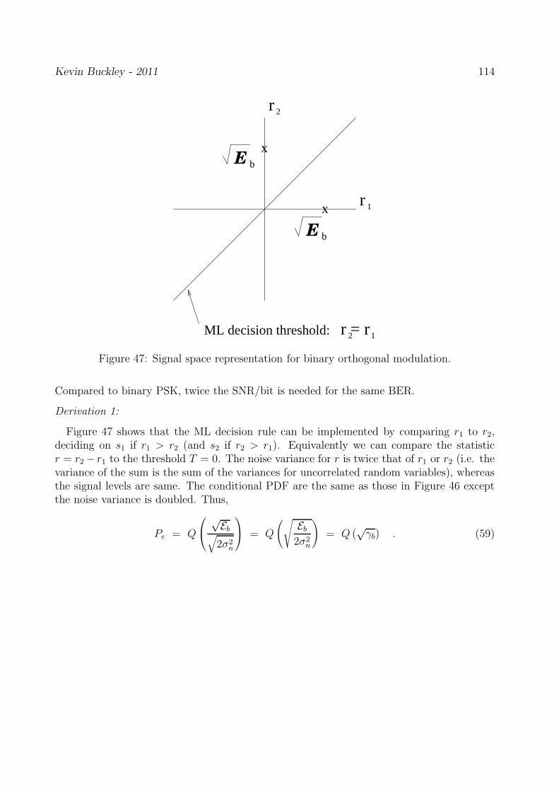
Kevin Buckley - 2011 114
E b
E b
r 1
r 2
r = r2 1
x
x
ML decision threshold:
Figure 47: Signal space representation for binary orthogonal modulation.
Compared to binary PSK, twice the SNR/bit is needed for the same BER.
Derivation 1:
Figure 47 shows that the ML decision rule can be implemented by comparing r1 to r2,deciding on s1 if r1 > r2 (and s2 if r2 > r1). Equivalently we can compare the statisticr = r2− r1 to the threshold T = 0. The noise variance for r is twice that of r1 or r2 (i.e. thevariance of the sum is the sum of the variances for uncorrelated random variables), whereasthe signal levels are same. The conditional PDF are the same as those in Figure 46 exceptthe noise variance is doubled. Thus,
Pe = Q
√Eb√
2σ2n
= Q
(√
Eb2σ2
n
)
= Q (√γb) . (59)
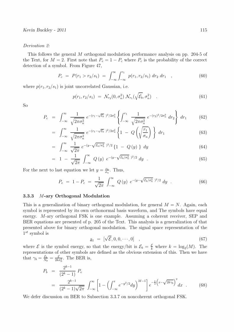
Kevin Buckley - 2011 115
Derivation 2:
This follows the general M orthogonal modulation performance analysis on pp. 204-5 ofthe Text, for M = 2. First note that Pe = 1 − Pc where Pc is the probability of the correctdetection of a symbol. From Figure 47,
Pc = P (r1 > r2/s1) =∫ ∞
−∞
∫ r1
−∞p(r1, r2/s1) dr2 dr1 , (60)
where p(r1, r2/s1) is joint uncorrelated Gaussian, i.e.
p(r1, r2/s1) = Nr2(0, σ2n) Nr1(
√
Eb, σ2n) . (61)
So
Pc =∫ ∞
−∞
1√
2πσ2n
e−(r1−√Eb )2/2σ2
n
∫ r1
−∞
1√
2πσ2n
e−(r2)2/2σ2n dr2
dr1 (62)
=∫ ∞
−∞
1√
2πσ2n
e−(r1−√Eb )2/2σ2
n
1 − Q
(√
r1σn
)
dr1 (63)
=∫ ∞
−∞
1√2π
e−(y−√
Eb/σ2n )2/2 1 − Q (y) dy (64)
= 1 − 1√2π
∫ ∞
−∞Q (y) e−(y−
√Eb/σ2
n )2/2 dy . (65)
For the next to last equation we let y = r1σn. Thus,
Pe = 1− Pc =1√2π
∫ ∞
−∞Q (y) e−(y−
√Eb/σ2
n )2/2 dy . (66)
3.3.3 M-ary Orthogonal Modulation
This is a generalization of binary orthogonal modulation, for general M = N . Again, eachsymbol is represented by its own orthonormal basis waveform, and The symbols have equalenergy. M-ary orthogonal FSK is one example. Assuming a coherent receiver, SEP andBER equations are presented of p. 205 of the Text. This analysis is a generalization of thatpresented above for binary orthogonal modulation. The signal space representation of the1st symbol is
s1 = [√E , 0, 0, · · · , 0] , (67)
where E is the symbol energy, so that the energy/bit is Eb = Ekwhere k = log2(M). The
representations of other symbols are defined as the obvious extension of this. Then we havethat γb =
EbN0
= E2kσ2
n. The BER is,
Pb =2k−1
(2k − 1)Pe
=2k−1
(2k − 1)√2π
∫ ∞
−∞
[
1−(∫ x
−∞e−y2/2dy
)M−1]
e− 1
2
(
x−√
2kγb
)2
dx . (68)
We defer discussion on BER to Subsection 3.3.7 on noncoherent orthogonal FSK.

Kevin Buckley - 2011 116
3.3.4 M-ary PSK
Analysis of M-ary PSK for a coherent receiver is presented in pp. 190-5 of the Text. Forthis modulation scheme, the signal space representations are
sm =[√
E cos (2π(m− 1)/M) ,√E sin (2π(m− 1)/M)
]T; m = 1, 2, · · · ,M (69)
where E is the symbol energy. The symbol error probability is
Pe = 1 −∫ π/M
−π/MpΘ(θ) dθ , (70)
where Θ is the observation signal space representation vector phase, under the m = 1assumption, which has PDF
pΘ(θ) =1
2πe−kγb sin
2 θ∫ ∞
0v e−(v−
√2kγb cos θ)
2/2 dv , (71)
where V is the vector magnitude random variable and γb is SNR/bit. For M = 2, Pe reducesto the 2-PSK equation derived earlier. For M = 4, it can be shown that
Pe = 2 Q(
√
2γb
) [
1 − 1
2Q(
√
2γb
)]
. (72)
For M > 4, Pe can obtained by evaluating Eq (70) numerically. The approximation,
Pe ≈ 2 Q(
√
2kγb sin(π/M))
, (73)
is derived in the Text on p. 194. As pointed out on p. 195, for Gray code bit to symbolmapping,
Pb ≈ 1
kPe . (74)
3.3.5 M-ary PAM
Performance for this N = 1 dimensional modulation scheme, with coherent reception, ispresented on pp. 188-90 of the For this modulation scheme, the signal space representationsare
sm = (2m− 1−M) d
√
Eg2
; m = 1, 2, · · · ,M , (75)
and the average energy/symbol is
Eav =1
6(M2 − 1) d2 Eg . (76)
The average probability of symbol error is
Pe =2(M − 1)
MQ
√
6 k γb,avM2 − 1
(77)
where γb,av =Eb,avN0
and Eb,av = Eavk. Note that BER is not given since, unlike the M-ary
orthogonal modulation case, it is a complicated calculation which depends on how the bitsvalues are assigned to the different symbols.

Kevin Buckley - 2011 117
3.3.6 M-ary QAM
Performance of QAM with coherent reception is considered in Subsection 4.3-3 of the Text.For this modulation scheme, the signal space representations are
sm =
√
Eg2
Vm cos θm ,
√
Eg2
Vm sin θm
T
. (78)
If the constellation of symbol points is on square grid, and if k is even (i.e. for 4-QAM, 16-QAM, 64-QAM ... ), then QAM can be interpreted as two
√M -ary PAM modulations, one
on the in-phase basis and the other on the quadrature. For correct detection, both in-phaseand quadrature must be detected correctly. So the symbol error probability is
Pe = 1 − (1− Pe,√M)2 , (79)
where Pe,√M is the SEP for
√M -ary PAM, i.e. from Eq 77,
Pe,√M =
2(√M − 1)√M
Q
√
3kγb,avM − 1
, (80)
and γb,av is the average SNR/bit. As with M-PAM, in general for QAM it is difficultdetermine an expression for Pb.
3.3.7 M-ary Orthogonal FSK Modulation
Now we consider noncoherent reception ofM-ary orthogonal FSK. For coherent reception, wehave already considered this modulation scheme in Subsection 3.3.3. Assume M equiprob-able, equal energy orthogonal FSK symbols. In pp. 216-218 of the Text, symbol errorprobability is shown to be
Pe =M−1∑
n=1
(−1)n+1
(
M − 1n
)
1
n + 1e−
nkγbn+1 . (81)
Concerning BER, first let P (i/j) denote the probability of deciding symbol i given symbol jwas transmitted. Note that with orthogonal modulation, all p(i/j); i 6= j are equal. Thus,
P (i/j) =Pe
M − 1=
Pe
2k − 1i 6= j . (82)
For any bit represented by any transmitted symbol, there are 2k−1 other symbols that, ifincorrectly detected, will result in an error in that bit. Orthogonal symbol errors events areindependent, the probability of error of that bit is the sum of the individual probabilities ofevents resulting in that bit being in error. So, for equally probable bits,
Pb = 2k−1 Pe
2k − 1≈ 1
2Pe . (83)

Kevin Buckley - 2011 118
3.3.8 Examples of Performance Analysis
Example 3.7: For M-ary orthogonal modulation, determine the SNR/bit required to achieveBER = 10−4 for M = 2 and M = 64. Then, Using the union/Chernov bound on Pe derivedin the Text on pp. 206-7, determine a bound on SNR/bit, γb, that assures Pe −→ 0 asM −→ ∞.
Solution: Using the orthogonal modulation Pe vs. γb plot in the Text, Figure 4.4-1 onp. 206, we get that, to achieve BER = 10−4 for M = 2 we need γb = 11dB. For M = 64we need γb = 5.8dB. With M = 64 we save 5.2dB in SNR/bit to achieve the same level ofperformance. Of course, in this case the price paid would be a significantly larger bandwidth(e.g. M = 2 FSK vs. M = 64 FSK). Considering the union/Chernov bound
Pe < e−k(γb − 2 ln 2)/2 (84)
(i.e. Eq. 4.4-17from the Course Text), note that as k −→ ∞ (i.eM −→ ∞), Pe −→ 0 as longas γb > 2 ln 2 = 1.42dB. In words, we can assure reliable communications (arbitrarily lowPe) using orthogonal symbols, as long as the SNR/bit is greater than 1.42dB (and assumingwe are willing to use a lot of orthogonal symbols). This leads to two important questions:1) Is this bound tight, or can we achieve reliable communications at lower SNR/bit? and 2)Can we achieve reliable communications at this SNR/bit level, or better, without having toresort to large numbers of orthogonal symbols? These questions have motivated extensiveresearch over the past 60 years. As established in ECE8771, the answer to the first questionis that this bound is not very tight. We will also see that the answer to the second questionis yes, there are more practical approaches to achieving performance close to even tighterperformance bounds.
Example 3.8: Figure 48 shows performance curves for several digital modulation schemeswith ML symbol detection and coherent reception. These plots, of symbol error probabilityvs. SNR/bit, were generated using the performance equations presented in this Subsection.Comparing binary PAM with binary orthogonal symbols, binary PAM performs γb = 3dBbetter for any level of performance. Also, for SEP at moderate (e.g. 10−3) to very good (e.g.< 10−6) levels, 8-PAM requires about 8dB more SNR/bit.
0 5 10 15 2010
−6
10−5
10−4
10−3
10−2
10−1
100
SNR/bit − γb (dB)
SE
P (
BE
R fo
r M
=2)
−−−−−−−−−−− binary PAM
− − − − − − binary orthogonal
.......... QPSK
− . − . − . 8−PAM
Figure 48: Performance curves for several modulation schemes.

Kevin Buckley - 2011 119
3.3.9 A Performance/SNR/Bandwidth Comparison of Modulation Schemes
In the selection of channel codes to control symbol errors, bandwidth and power requirementsare important considerations. For a given channel noise level, the power requirement isequivalent to an SNR requirement. SNR and bandwidth requirements differ for differentmodulation schemes.
In Subsection 3.3.1-8 we summarized symbol and bit error rates vs. SNR for several linear,memoryless modulation schemes. Earlier in the Course, in Subsection 1.4.9, we developeda foundation from which bandwidth characteristics of different modulation schemes can bederived. Some useful approximate bandwidth requirements are stated in Subsection 4.6 ofText, and summarized in the table below. W is the approximate bandwidth, in Hz., and Ris the bit rate.
Modulation Bandwidth W Bite Rate R R/W
PAM (SSB) 12T
1Tk = 1
Tlog2M 2 log2M
PSK 1T
1Tk = 1
Tlog2M log2M
QAM 1T
1Tk = 1
Tlog2M log2M
FSK M2T
1Tk = 1
Tlog2M
2 log2 MM
Table 3.1: Approximate Bandwidth Requirements for Different ModulationSchemes.
A performance quantity of principal concern in digital communication systems is band-width efficiency, which is the rate-to-bandwidth ratio
R
W(85)
with units (bits/sec./Hz.). Bandwidth efficiency tells us how many bits per second we canpush through the system per Hertz of system bandwidth. Figure 4.6-1 Text (reproducedbelow as Figure 49) compares, for a symbol error rate of 10−5, efficiency for some of themodulation schemes we’ve considered. The channel capacity bound and its asymptotic valueare topics of ECE8771. The relevance of the “bandwidth-limited region” R
W> 1 and the
“power-limited region” RW
< 1 becomes more clear when studing tellis coded modulation inECE8771.

Kevin Buckley - 2011 120
orthogonal symbols (coherent)
bandwidth efficient region
5 10 15 20
2
3
5
10
0.1
0.2
0.3
0.5
channel capacity
C/W
−1.6
asymptoticM=8
M=16
M=32
M=64
M=4
M=8
M=2
R/W (bits/sec/Hz)
SNR/bit (dB)
M=8M=4
QPSKM=2 PAM
M=2
PAM (coherent)
PSK (coherent)
Differential PSK
power efficient region
Figure 49: Comparison of SNR and bandwidth characteristics of several modulation schemesat SEP = 10−5.


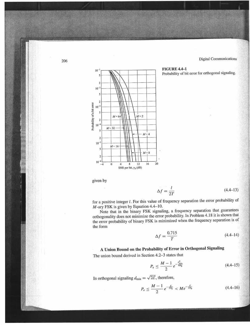


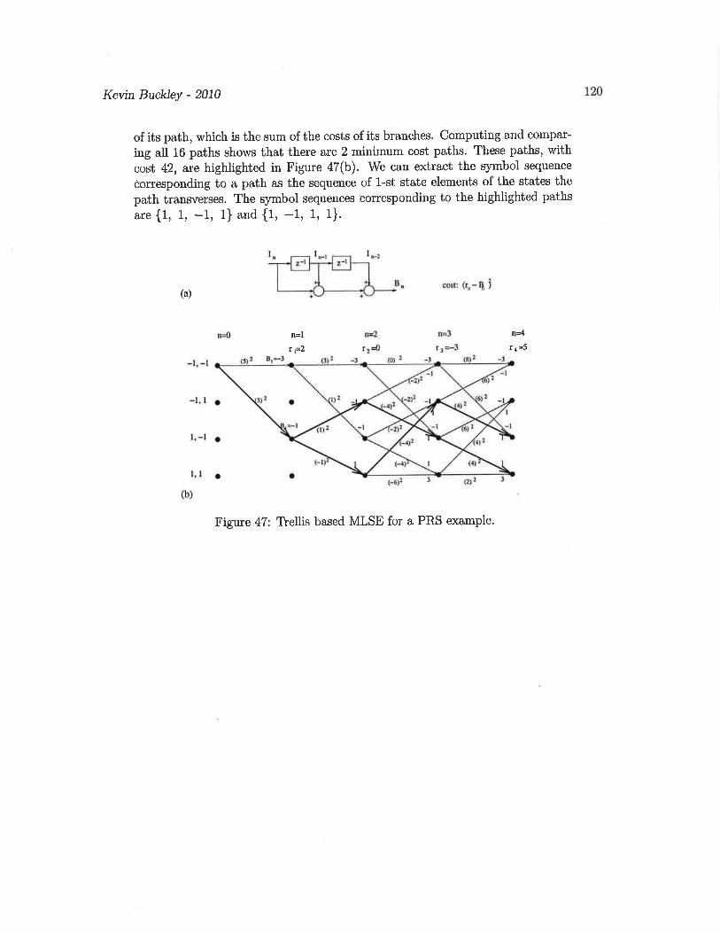


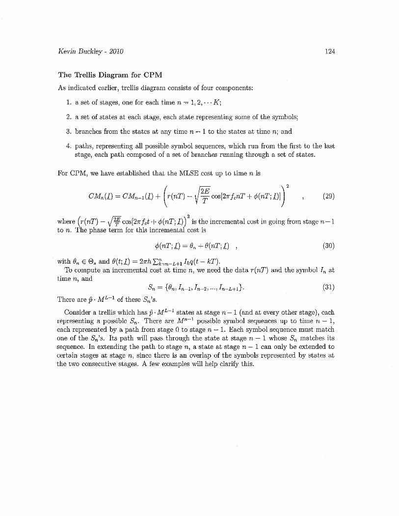
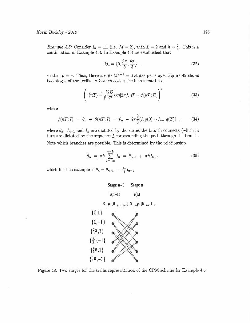


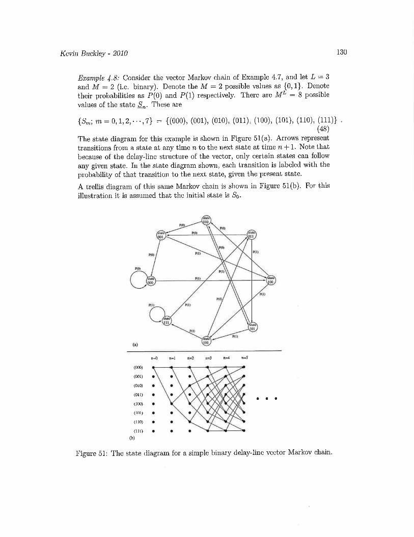


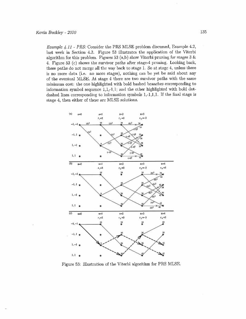


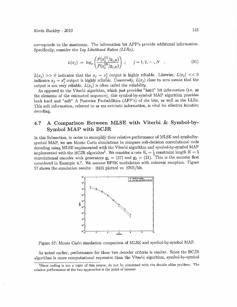
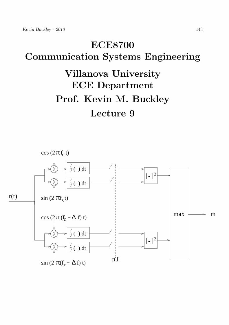
Kevin Buckley - 2010 143
ECE8700Communication Systems Engineering
Villanova UniversityECE Department
Prof. Kevin M. Buckley
Lecture 9
cos (2 f t)cπ
cπsin (2 f t)
π c ∆cos (2 (f + f) t)
π c ∆sin (2 (f + f) t)
( ) dt
( ) dt
( ) dt
( ) dt
| |. 2
| |. 2
nT
mmax
r(t)
Kevin Buckley - 2010 144
Contents
5 Noncoherent Detection & Synchronization 1455.1 Reception with Carrier Phase and Symbol Timing Uncertainty . . . . . . . . 1455.2 Noncoherent Detection . . . . . . . . . . . . . . . . . . . . . . . . . . . . . . 1485.3 From ML/MAP Detection to ML/MAP Parameter Estimation . . . . . . . . 1535.4 Carrier Phase Estimation . . . . . . . . . . . . . . . . . . . . . . . . . . . . . 1555.5 Symbol Timing Estimation . . . . . . . . . . . . . . . . . . . . . . . . . . . . 1565.6 Joint Carrier Phase and Symbol Timing Estimation . . . . . . . . . . . . . . 158
List of Figures
58 Digital communication receiver – receiver filter/demodulator and detector. . 14559 Bandpass and equivalent lowpass implementations of a correlator receiver. . 14660 Envelope detector for optimum noncoherent reception. . . . . . . . . . . . . 14961 Square-law detector for optimum noncoherent reception. . . . . . . . . . . . 15062 Square-law detector for optimum noncoherent reception of M = 2 FSK. . . . 15063 A nonsynchronous binary DPSK receiver. . . . . . . . . . . . . . . . . . . . . 15164 A Phase-Locked Loop (PLL) for recovery of an unmodulated carrier. . . . . 15565 A Timing-Locked Loop (TLL) for recovery of symbol timing. . . . . . . . . . 156

Kevin Buckley - 2010 145
5 Noncoherent Detection & Synchronization
In this Section of the Course we address two common types of digital receiver uncertainty:carrier phase uncertainty, and symbol timing uncertainty. These result due to propagationdelay through the channel. One basic approach to dealing with the uncertainty of the carrierphase and symbol timing parameters is to transmit additional signal components, in additionto the communication signal, which facilitates the derivation of these parameters at thereceiver. This approach, while important, requires additional resources (e.g. transmit power,bandwidth). The other basic approach is to deal with these uncertainties at the receiver usingthe received communication signal itself. In this Section we discuss this latter apporach. Wedetail the problem in Section 5.1. We discuss the noncoherent receiver approach to thecarrier phase uncertainty problem in Section 5.2. In Section 5.3 through 5.5 we considerestimation of the carrier phase and symbol timing parameters.
5.1 Reception with Carrier Phase and Symbol Timing Uncer-tainty
Consider a set of symbols sm(t); m = 1, 2, · · · , M ; 0 < t ≤ T , with sm(n)(t) received atsymbol time n in AWGN. Recall that given the received signal
r(t) = sm(t) + n(t) ; 0 < t ≤ T (1)
the symbol detection objective is to decide which of the M symbols was transmitted. Figure58 depicts the problem. The receiver front-end (i.e. the modulation scheme correlator ormatched filter) demodulates the received signal and filters it prior to detection or sequenceestimation.
r
s (t)m(n)
I n
n(t)
r(t)
T
receiverfront−end
decision device(e.g. threshold detector)
Figure 58: Digital communication receiver – receiver filter/demodulator and detector.
In Section 3.1 of this Course, we described the correlator receiver, provided some justifica-tion for it, established its sampled output characteristics, and showed its equivalence to thematched filter receiver. This receiver structure correlates the received signal r(t); 0 < t ≤ Twith each of the modulation scheme basis functions, φk(t); k = 1, 2, · · · , N , of the givenmodulation scheme. This correlation is the inner product, so the correlation receiver forms
r = [r1, r2, · · · , rN ]T (2)
where N is the modulation scheme dimension and
rk = < r(t), φk(t) > =∫ T
0r(t) φk(t) dt k = 1, 2, · · · , N (3)
=1
2Re< rl(t), φkl(t) > =
∫ T
0rl(t) φ∗
kl(t) dt (4)

Kevin Buckley - 2010 146
where rl(t) is the lowpass equivalent (e.g. quadrature receiver output) of r(t) and the φkl(t)are the lowpass equivalent basis functions. Figures 59(a,b) show, respectively, the bandpassand equivalent lowpass implementations. In the bandpass implementation illustration, notethat the multiplication of r(t) by the φk(t) represents the demodulation process, since theφk(t) are bandpass functions (typically cosines with an envelope shaped by a pulse shapeg(t)). The integrator is effectively a lowpass filter. The integrator output is sampled whenthe symbol fills the integrator. For the lowpass equivalent implementation illustration, notethe demodulation has already taken place.
r 1
r N
lr (t)
r
0
T( . ) dt
21
0
T( . ) dt
21 Re
Re
1,l
(b)
.....
.....
N,l
(t)
(t)
φ
φ
*
*
r
0
T( . ) dt 1r
0
T( . ) dt
r N
.....
.....
r(t)
(t)
(t)
φ
φ
1
N
(a)
Figure 59: Bandpass and equivalent lowpass implementations of a correlator receiver.
There are two implied assumptions in this receiver that often are not met in application:
1. It is assumed that the basis functions, the φk(t) are exactly known to the receiver.Given that we know what the modulation scheme is, this does not on the surface seemlike an unreasonable assumption. For the bandpass transmission, these basis functionsare similar in form to
φ(t) =
√
2
Egg(t) cos(2πfct) . (5)
The sinusoid cos(2πfct) is called the carrier. The pulse shape g(t) and carrier frequencyfc are system specifications. So they can be assumed to be known1 The received pulseenergy, Eg, may be a problem, for example when carrier is amplitude modulated, butAutomatic Gain Control (AGC) can be employed to effectively deal with this.
However, note that the carrier phase is implied to be zero. Basically, this means thatit is assumed that the carrier phase as observed at the receiver is known. Given thatthere is an unknown channel delay, this will not be the case in practice. There is carrierphase uncertainty at the receiver. Below we present several examples of the undesirableconsequence of carrier phase uncertainty. So, in any practical digital communicationsystem, this problem must be addressed.
Assuming and employing this knowledge of the carrier phase at the receiver is referredto as coherent reception. For a coherent receiver, then, we must somehow recover thecarrier phase. The process for achieving this is termed carrier phase estimation orcarrier synchronization. An alternative receiver strategy can be implemented – one
1Although there will inevitably be some slight offset between the transmitter and receiver carrier fre-
quency, we will see that this is accounted for by dealing with carrier phase uncertainty.

Kevin Buckley - 2010 147
that does not require carrier synchronization. Such a strategy is called noncoherentreception.
2. It is assumed that we know when to sample the correlator output – that we know whena symbol starts and stops. The symbol duration T is part of the system specification,so it is reasonable to assume it is known. So the assumption reduces to that of knowingwhen each symbol starts. Again because in practice there is an unknown delay thoughtthe channel, this assumption is not reasonable. There will be symbol timing uncertainty,and thus there is a need for symbol timing recovery. The process for achieving this istermed symbol time estimation or symbol synchronization.
Examples of the carrier phase uncertainty problem:
As an obvious example, first consider M-ary PSK. A transmitted symbol is of the form
sm(t) =
√
2
Egg(t) cos(2πfct + θm) 0 < t ≤ T , (6)
where θm = 2πM
m; m = 0, 1, · · · , M − 1. Assume that the received signal is
r(t) =
√
2
Egg(t) cos(2πfct + θm + φ) + n(t) 0 < t ≤ T , (7)
where φ is an unknown phase shift due to the channel. Clearly, since the receiver objectiveis to determine θm, the unknown receiver carrier phase φ is a problem. For example, if φis ignored, and it has a value of say 2π
M, then even with no noise the incorrect phase will be
detected at the receiver. Carrier phase uncertainty can be a problem for any modulationscheme for which information is embedded in the carrier phase (e.g. PSK, QAM).
As another example, consider the PAM problem described on p. 295 of the Course Text.Let
s(t) = A(t) cos(2πfct + φ) (8)
be the received PAM signal, where φ is an unknown phase shift introduced by the channel.For the correlation receiver, let the PAM basis function be
φ(t) =
√
2
Tcos(2πfct + φ) (9)
where φ is the assumed carrier phase at the receiver. The correlation receiver multiplieroutput is
s(t) φ(t) =
√
2
TA(t) cos(2πfct + φ) cos(2πfct + φ) (10)
=
√
1
2TA(t)
[
cos(φ − φ) + cos(4πfct + (φ + φ))]
. (11)

Kevin Buckley - 2010 148
Since the correlator receiver integrator is effectively a lowpass filter, at its output the 4πfc
sinusoidal term is attenuated. The remaining term is
y(t) =
√
1
2TA(t) cos(φ − φ) . (12)
The error between the assumed and actual carrier phase is manifested as cos(φ − φ). Thissuggests that at the correlator receiver output the received symbol can be substantiallyattenuated. For example, if φ − φ = π
2, y(t) = 0.
5.2 Noncoherent Detection
Noncoherent detection is covered in depth in Section 4.5 of the Course Text. Therein, opti-mum noncoherent detection is formulated in general, a general optimum detector structureis identified, several modulation schemes are considered, and performance is analyzed. Here,we overview selected discussions from that Section.
Noncoherent Detection of Carrier Modulated Signals
Consider and digital modulation scheme for which the symbols can be represented as
sm(t) = Re
sml(t) ej2πfct
(13)
where sml(t) is the lowpass equivalent. This includes PAM, PSK, QAM and some binaryorthogonal schemes such as FSK. Let the received signal due to a transmitted symbol sm(t)be of the form
r(t) = sm(t − td) + n(t) , (14)
or equivalentlyrl(t) = Re
sml(t − td) e−j2πφ ej2πfct
(15)
where td is an unknown channel induced delay2 and φ = fctd. Assume that sml(t − td) ≈sml(t). This implies that either td << T (where T is the symbol duration) or symbolsynchronization has been implemented. Then, the lowpass equivalent of the received symbolis
rl(t) = ejφ sml(t) + nl(t) , (16)
with complex signal space vector representation
rl = ejφ sml + nl (17)
(i.e. rl = rrl + jril is the complex representation of 2-dimensional rl = [rrl, ril]T ). For
the ML or MAP symbol detection problem formulation, we need prl(rl/sml), the PDF of rl
conditioned on sml. For this, we start with the joint PDf of rl and φ, and marginalize overφ. Letting pφ(φ) denote the prior PDF of random φ,
prl(rl/sml) =
∫
prl,φ(rl, φ/sml) dφ (18)
=∫
pnl(rl − sml) pφ(φ/sml) dφ =
∫
pnl(rl − sml) pφ(φ) dφ (19)
2For this discussion we do not explicitly address channel attenuation, which would be incorporated into
the SNR and controlled with AGC. We do not address multipath channels until later in the course.

Kevin Buckley - 2010 149
where pnl(nl) is the noise PDF, and we assume that, conditioned on sml, the noise nl and
phase φ are statistically independent, and that φ does not depend on sml. The MAP symboldetection problem is then
maxm
Pm
∫
pn(rl − sml) p(φ) dφ (20)
where Pm is the probability of the m-th symbol. It is shown in Subsection 4.5-1 of the CourseText that in terms of the lowpass equivalent received signal, assuming AWGN and the priordistribution on φ is uniform over 2π, this MAP problem reduces to
maxm
Pm e−Em/2N0 I0
(
|rl · sml|2N0
)
(21)
where N0 is the noise spectral level, Em is the energy of the m-th symbols, and I0(x) is themodified Bessel function of the first kind and order zero. Since I0(x) is a monotonicallyincreasing function of x, for equiprobable and equi-energy symbols, this reduces to the moreintuitive problem:
maxm
|rl · sml| . (22)
Eq (22) suggests the optimum noncoherent detector illustrated below in Figure 60. Thedemodulator is a quadrature receiver. (This figure shows the receiver front end in terms offilters matched to the symbols as opposed to the equivalent structure based on correlationwith the modulation scheme basis functions.) This is referred to as an envelope detectorsince it selects the symbol corresponding to the maximum “envelope” |rl ·sml|. An equivalentdetector, referred to as a square-law detector, is illustrated in Figure 61.
s (T−t)2l*
*s (T−t)1l
*Mls (T−t)
| |.
| |.
| |.
1llr s.
Demodulatorr(t) r (t)l
nT
m
lr s.
lr s.
2l
Ml
max....
....
Figure 60: Envelope detector for optimum noncoherent reception.

Kevin Buckley - 2010 150
s (T−t)2l*
*s (T−t)1l
*Mls (T−t)
1llr s.
Demodulatorr(t) r (t)l
nT
m
lr s.
lr s.
2l
Ml
max....
....
| |.
| |.
| |. 2
2
2
Figure 61: Square-law detector for optimum noncoherent reception.
Noncoherent Decoding of FSK
As a special case of the noncoherent demodulator developed above, consider FSK for whichthe symbols are
sm(t) = g(t) cos(2πfct + 2π(m − 1) ∆f t) ; m = 1, 2, · · · , M . (23)
The square-law detector, in terms of the bandpass symbols, is illustrated in Figure 62 forM = 2 symbols.
cos (2 f t)cπ
cπsin (2 f t)
π c ∆cos (2 (f + f) t)
π c ∆sin (2 (f + f) t)
( ) dt
( ) dt
( ) dt
( ) dt
| |. 2
| |. 2
nT
mmax
r(t)
Figure 62: Square-law detector for optimum noncoherent reception of M = 2 FSK.

Kevin Buckley - 2010 151
Noncoherent Decoding of DPSK
Earlier in the Course we introduced binary DPSK as an example of a modulation schemewith memory and noted that one advantage of it is that it facilitates decoding withoutknowledge of the carrier phase – i.e. noncoherent reception is possible by simply detectingthe change in initial phase from symbol to symbol. Here we describe a DPSK receiver thatdoes not require carrier synchronization.
As we saw in Section 4 of the Course Notes, since DPSK is a modulation scheme withmemory, optimum (ML or MAP) estimation of a symbol sequence requires the joint pro-cessing of all the symbols in the sequence and all the observed data over the extent of thesequence. In other words, decoupled symbol-by-symbol detection as described in this Sub-section is not optimum. Note that an alternative noncoherent detection scheme for DPSKis described in Subsection 4.5-5 of the Course Text.
Consider binary DPSK, where the transmitted signal is observed at the receiver withunknown phase φ in AWGN. The received signal over the kth symbol duration is
r(t) = g(t) cos(2πfct + θk + φ) + n(t) kT < t ≤ (k + 1)T (24)
where θk is 0 or π depending on what the kth symbol is and what all the previous symbolswere. Consider DPSK and the demodulator depicted in Figure 63.
kT
(k+1)T ( . ) dt
kT
(k+1)T ( . ) dt
2Eg
πg(t) cos(2 f t)c
2Eg
π cg(t) sin(2 f t)
r k,r
r k,i
T
rr(t) r
r
k
k−1
(k+1)T
Figure 63: A nonsynchronous binary DPSK receiver.
Two correlators are used instead of the one normally required for binary PSK because,with unknown phase φ at the receiver, g(t) cos(2πfct + θk + φ) is two dimensional over0 < φ ≤ 2π (i.e. two basis functions are required to represent it over the range of unknownφ). The 2-dimensional observation vector for symbol k is
rk = [rk,r, rk,i] = [√
Es cos(θk − φ) + nk,r,√
Es sin(θk − φ) + nk,i] (25)

Kevin Buckley - 2010 152
where Es is the symbol energy (i.e. for binary modulation schemes Es is the same as the bitenergy Eb). Eq. (25) can also be conveniently thought of as the complex-valued observation
rk = rk,r + jrk,i =√
Es ej cos(θk−φ) + nk , (26)
where nk = nk,r + jnk,i.If, as shown in Figure 63, we form the produce rkr
∗
k−1, then as explained in Subsection5.2.8 of the Course Text, for binary DPSK
rkr∗
k−1√Es
≈ xk + jyk (27)
where xk and yk are real-valued (i.e. xk is the real part of rkr∗
k−1) and
xk = ±√
Es + Renk + n∗
k−1 (28)
yk = Imnk + n∗
k−1 . (29)
The noise in yk is statistically independent of that in xk, so that only xk need be processed.In xk, a
√Es indicates a ”0” bit while a −
√Es indicates a ”1”. xk has the same form as
regular (coherent) PSK, except the noise has twice the power. Thus, compared to binaryPSK, performance of binary DPSK using this decoding approach will by (approximately)3dB worse.

Kevin Buckley - 2010 153
5.3 From ML/MAP Detection to ML/MAP Parameter Estima-tion
Recall the maximum likelihood symbol detection problem addressed in Section 3.2 of thisCourse. Starting with the signal space representation of the received data for an N -dimensionalmodulation scheme, the N -dimensional vector r, and the M symbol signal space represen-tation vectors, the sm; m = 1, 2, · · · , M , the ML problem is:
maxsm
p(r/sm) (30)
where p(r/sm) is the likelihood function (i.e. the data vector joint PDF, conditioned ofsymbol sm having been transmitted, with the received data vector r plugged in). Under theAWGN assumption, this becomes
maxsm
p(r/sm) =1
(2π)N/2(σ2n)N/2
e−∑
N
k=1(rk−smk)2/2σ2
n , (31)
or equivalently,
minsm
N∑
k=1
(rk − smk)2 = ||r − sm||2 . (32)
This is just the minimum distance decision rule, which suggests a particularly simple MLsymbol detection algorithm.
The MAP detector is based on the posterior PDF P (sm/r) of sm given r. Using Bayesrule, we have
P (sm/r) =p(r/sm)P (sm)
p(r)(33)
where P (sm) is the probability of sm, and p(r) is the joint PDF of r. The MAP detectorconsists of the following two steps:
1. Plug the available data r into p(sm/r). Consider the result to be a function of sm, thesymbol parameters to be detected.
2. Determine the symbol sm that maximizes this function. This symbol is the MAPdetection.
Since the denominator term in Eq. 33 is independent of sm, the MAP detector can be statedas:
maxsm
p(r/sm) P (sm) . (34)
Comparing Eqs. 30 and 34, we see that the difference lies in the MAP detector’s weightingof the likelihood function by the symbol probabilities P (sm). If the symbols are equallylikely, then the ML and MAP detectors are equal. However, in general they aredifferent. In terms of the primary objective of symbol detection, the MAP estimator isoptimum in that it minimizes symbol error rate. The MAP detector is a little harderto design, but just as easily implemented.

Kevin Buckley - 2010 154
In Section 4 of the Course we saw that the Maximum Likelihood Sequence Estimation(MLSE) formulation is a straightforward extension of ML detection, though algorithmically itis more challenging. MAP sequence estimation is a similar generalization of MAP detection.
We can consider these ML and MAP symbol detection and sequenceestimation problemsto be discrete-valued parameter estimation problems. The resulting algorithms all involvesearching for the lowest cost from a countably finite number of possible solutions. We nowturn our attention to ML and MAP estimation of the carrier phase φ and symbol delay τ .The objective is to identify good estimates of these two parameters and to then use themto do coherent detection so as to realize the performance advantage of coherent detectioncompared to noncoherent detection. φ and τ are continuous-valued parameters. We will seethat the ML and MAP estimator problem formulations for these parameters are identicalto those for a discrete-valued parameter (e.g. symbol detection) problem. However, theresulting algorithms will be substantially different, due to the need to select the lowest costover a continuum of possible solutions.
Let θ denote the continuous-valued parameter or parameter vector of interest, i.e. θ isφ or τ or φ, τ. Let r generally denote the data. Given data r, with joint PDF p(r/θ)conditioned on a value of θ, the ML parameter estimation problem is:
maxθ
L(θ) = p(r/θ) (35)
where L(θ) is the likelihood function (the data conditional PDF with the data plugged in).The MAP parameter estimation problem is:
maxθ
p(θ/r) =p(r/θ) p(θ)
p(r).= p(r/θ) p(θ) , (36)
where p(θ) is the known prior PDF of θ. Note that if p(θ) is constant over the range of θ ofinterest, the ML an MAP estimates are the same.
The exact form of the MAP (or ML) problem formulation and resulting processing algo-rithm will depend of what form the data takes on. In Subsection 5.1-1 of the Course Text,the authors start with the received data waveform r(t) over a symbol period T . For thisdata, they show that the likelihood function is equivalent to
Λ(θ) = exp
− 1
N0
∫
T|r(t) − s(t; θ)|2 dt
, (37)
where s(t; θ) would be the received symbol, given θ, if there were no noise.In Subsection 5.1-2 of the Course Text, the authors illustrate receiver block diagrams which
account for carrier phase and symbol timing uncertainty for several modulation schemes (i.e.binary PSK, M-ary PSK, M-ary PAM and general QAM). These diagrams each includesa carrier recovery block and a symbol synchronization block. These blocks implement, re-spectively, the φ and τ parameter estimators. We now use ML/MAP formulations to designthese blocks. The PAM and QAM diagrams incorporate Automatic Gain Control (AGC).AGC compensates to unknown channel attenuation. This issue is not addressed in the CourseText, so we will not address it here. Note, however, that the AGC block can also be designedusing a ML or MAP formulation (for the estimation of a channel attenuation factor).
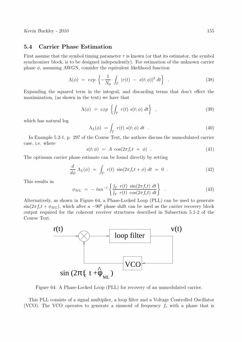
Kevin Buckley - 2010 155
5.4 Carrier Phase Estimation
First assume that the symbol timing parameter τ is known (or that its estimator, the symbolsynchronizer block, is to be designed independently). For estimation of the unknown carrierphase φ, assuming AWGN, consider the equivalent likelihood function
Λ(φ) = exp
− 1
N0
∫
T|r(t) − s(t; φ)|2 dt
. (38)
Expanding the squared term in the integral, and discarding terms that don’t effect themaximization, (as shown in the text) we have that
Λ(φ).= exp
∫
Tr(t) s(t; φ) dt
, (39)
which has natural log
ΛL(φ) =∫
Tr(t) s(t; φ) dt . (40)
In Example 5.2-1, p. 297 of the Course Text, the authors discuss the unmodulated carriercase, i.e. where
s(t; φ) = A cos(2πfct + φ) . (41)
The optimum carrier phase estimate can be found directly by setting
d
dφΛL(φ) =
∫
Tr(t) sin(2πfct + φ) dt = 0 . (42)
This results in
φML = − tan−1
∫
T r(t) sin(2πfct) dt∫
T r(t) cos(2πfct) dt
. (43)
Alternatively, as shown in Figure 64, a Phase-Locked Loop (PLL) can be used to generatesin(2πfct + φML), which after a −900 phase shift can be used as the carrier recovery blockoutput required for the coherent receiver structures described in Subsection 5.1-2 of theCourse Text.
π φc MLsin (2 f t + )^
r(t) loop filter
VCO
v(t)
Figure 64: A Phase-Locked Loop (PLL) for recovery of an unmodulated carrier.
This PLL consists of a signal multiplier, a loop filter and a Voltage Controlled Oscillator(VCO). The VCO operates to generate a sinusoid of frequency fc with a phase that is

Kevin Buckley - 2010 156
proportional to the integral of the VCO input v(t). The PLL operates to provide a VCOoutput that results in the VCO input v(t) = 0. This is, it drives the VCO input to zero. Adetailed analysis of this PLL, which can be found in Subsections 5.2-2 and 5.2-3 of the Text,is beyond the scope of this Course.
Concerning unknown carrier phase φ, the real coherent receiver objective is carrier recoveryfrom the received modulated, noisy signal. Subsection 5.2-4 of the Course Text describesdecision-directed modification of the PLL to achieve this. This too is beyond the scope ofthis Course.
5.5 Symbol Timing Estimation
Now assume that the carrier phase φ is known (or that its estimator, the carrier recoveryblock, is to be designed independently). For estimation of the symbol timing parameterτ , assuming AWGN, consider the equivalent likelihood function in terms of lowpass signalrepresentation:
Λ(τ) = exp
− 1
N0
∫
T|rl(t) − sl(t; τ)|2 dt
, (44)
wheresl(t; τ) =
∑
n
In g(t − nT − τ) . (45)
Expanding the squared term in the integral, and discarding terms that don’t effect themaximization, (as shown in the text) we have that
Λ(τ).= exp
∫
Tr(t) s(t; τ) dt
, (46)
which has natural log
ΛL(τ) =∫
Tr(t) s(t; τ) dt =
∑
n
In yn(t) (47)
where yn(t) =∫
T rl(t) g(t− nT − τ) dt is the output of the receiver matched filter. For theML estimate, set
d
dτΛL(τ) =
∑
n
Ind
dτyn(t) = 0 . (48)
As shown in Figure 65, a Timing-Locked Loop (TLL) can be used to generate the MLmatched filter output sampling times.
adder
Matched Filter g(−t)
lr (t)
VCC
nT + τ ML
I n
differentiatorsampler
Figure 65: A Timing-Locked Loop (TLL) for recovery of symbol timing.

Kevin Buckley - 2010 157
This TLL consists of a matched filter, a sampler, a digital multiplier/summer, and aVoltage Controlled Clock (VCC). The TLL operates to provide a VCC output that drivesthe VCC input to zero. This TLL is called decision-directed because it employs “known”symbols at the receiver. These “known” signals are typically generated as the symbol detectoroutputs (i.e. the receiver outputs). Thus the term decision-directed.

Kevin Buckley - 2010 158
5.6 Joint Carrier Phase and Symbol Timing Estimation
A brief description of a coherent receiver approach based on ML estimation of both carrierphase φ and symbol timing parameter τ is presented in Section 5.4 of the Course Text. Thistopic is beyond the scope of this Course.

Kevin Buckley - 2010 157
ECE8700Communication Systems Engineering
Villanova UniversityECE Department
Prof. Kevin M. Buckley
Lecture 10
F (z )* −1A(z) = 1
vn
vn
f 0 f 1 f L
z−1 z−1 z−1I n
vn
η n
.....
I n
F(z)vn
η n
I n
(a)
ny
(b)
(c)
X(z) = F(z) F (z )−1*

Kevin Buckley - 2010 158
Contents
6 Bandlimited Channels and Intersymbol Interference 1596.1 The Digital Communication Channel and InterSymbol Interference (ISI) . . 1596.2 Signal Design and Partial Response Signaling (PRS) for Bandlimited Channels1646.3 A Discrete-Time ISI Channel Model . . . . . . . . . . . . . . . . . . . . . . . 1696.4 MLSE and the Viterbi Algorithm for ISI Channels . . . . . . . . . . . . . . . 177
List of Figures
66 Representations of a digital communication LTI ISI channel. . . . . . . . . . 16067 The lowpass equivalent channel output is the superposition of the individual
symbol outputs – i.e. the Inh(t − nT ). . . . . . . . . . . . . . . . . . . . . . 16268 (a) An ISI digital communication channel (lowpass equivalent shown); (b) an
equivalent discrete-time model. . . . . . . . . . . . . . . . . . . . . . . . . . 16569 Illustrations of the Nyquist Criterion of transmission of symbols without ISI
across a bandlimited channel. . . . . . . . . . . . . . . . . . . . . . . . . . . 16670 Orthogonal expansion of the lowpass equivalent received signal rl(t). . . . . . 16971 Equivalent discrete-time model of an ISI channel. . . . . . . . . . . . . . . . 17172 Equivalent discrete-time model of an ISI channel. . . . . . . . . . . . . . . . 17373 Whitening of the sampled matched filter output noise vn. . . . . . . . . . . . 17474 Zero configuration for the symmetric noncausal DT channel model. . . . . . 17575 DT ISI channel model including noise whitening. . . . . . . . . . . . . . . . 17676 DT ISI channel model including noise whitening. . . . . . . . . . . . . . . . 17777 ISI channel model, trellis diagram and Viterbi algorithm pruning for Example
6.2. . . . . . . . . . . . . . . . . . . . . . . . . . . . . . . . . . . . . . . . . . 18078 ISI channel model, trellis diagram & Viterbi algorithm pruning for Example
6.3. . . . . . . . . . . . . . . . . . . . . . . . . . . . . . . . . . . . . . . . . . 181

Kevin Buckley - 2010 159
6 Bandlimited Channels and Intersymbol Interference
In this Chapter of the Course we consider the effects of the digital communications channeland its mitigation. This corresponds to Chapter 9 of the Course Text. We assume that thechannel is linear and time invariant, and that the noise is AWGN. See Section 9.1, pp. 600-601 of the Course Text for brief discussions on non-linear channels, time-varying channels,frequency offset, phase jitter and impulses noise. Basically, carrier phase recovery techniquescan be used to combat frequency offset and phase jitter. Non-linear channels are beyond thescope of this course, as is impulsive noise which can be countered with channel coding. Time-varying channels are dealt with using adaptive techniques, which will be briefly discussed ina late Section of this Course.
The most important characteristic of any realistic communication channel is that it iseffectively bandlimited. In Section 6.1 we first describe a bandlimited, linear, time-invariantchannel, and we mathematically model interSymbol Interference (ISI) which is its primarydeleterious effect. In Section 6.2 we then introduce signal design methods for eliminating orcontrolling ISI. In Section 6.3 we then develop a discrete-time ISI model, which will be usedin Section 6.4 and in Chapter 7 to develop, respectively, MLSE and channel-equalizationtechniques for combating ISI at the receiver.
6.1 The Digital Communication Channel and InterSymbol Inter-ference (ISI)
This Section of the Course corresponds to Section 9.1 and the beginning of Section 9.2 ofthe Course Text.
The goal here is to develop an ISI model of a bandlimited digital communications channelthat will allow us to: 1) directly apply the MLSE techniques described previously in Chapter4 of this Course; and 2) develop channel equalization methods in Chapter 7. We will focuson MLSE for N = 1 and N = 2 dimensional linear modulation schemes. The approach easilyextends to higher dimensional and nonlinear schemes.
Consider QAM, for which PAM and PSK can be consider special cases. The lowpassequivalent symbols are sm(t); m = 1, 2, · · · , M :
sml(t) = Vmejθmg(t) ; 0 ≤ t ≤ T m = 1, 2, · · · , M , (1)
where g(t) is a real-valued pulse shape. For symbol time n and transmitted symbolm = m(n), we can represent the transmitted symbol as
sm(n)l(t − nT ) = Vm(n)ejθm(n) δ(t − nT ) ∗ g(t) (2)
where 1T
is the symbol rate and δ(t − nT ) is the impulse function delayed to time nT .In Section 2.6 of this Course, for a development of spectral characteristics of digitally
modulated signals, we established the following equivalent lowpass representation:In = In(n) = Vm(n)e
jθm(n) = Vmejθm. PAM, PSK and QAM where, respectively, In has form:
In = Am (3)
In = ej2π(m−1)/M
In = Vm ejφm .

Kevin Buckley - 2010 160
With this representation, the real part of In corresponds to the cosine basis function term onthe signal space representation, while the imaginary part corresponds to the sine term. ForPAM or 2-PSK, there would be no sine term (i.e. these are N = 1 dimensional modulationschemes). In is the random information sequence, for each symbol time n representingK = log2(M) bits.
Following the discussion and notation in Section 9.1 of the Course Text, consider thedigital communication channel illustrated as a lowpass equivalent in Figure 66(a). Using theIn representation of symbols, this illustration represents Mathematically, we can think of thelowpass equivalent modulator in this figure as effectively forming
I(t) =∑
n
In δ(t − nT ) (4)
and then processing it with an Linear Time-Invariant (LTI) filter with impulse response g(t).The lowpass equivalent of the transmitted signal is
v(t) = I(t) ∗ g(t) =∑
n
In g(t − nT ) , (5)
where actual (real-valued, bandpass) transmitted signal is
s(t) = Re v(t) ej2πfct . (6)
So, here r(t) and z(t) represent, respectively, the lowpass equivalent received signal andlowpass equivalent AWGN.
(b)
(a)
l
l
I n
v (t)
LTI Channel
h( t )
Modulator ( g(t) ) c( t )
LTI Channel
z (t)
z (t)
I (t)
r (t)
r (t)
Figure 66: Representations of a digital communication LTI ISI channel.
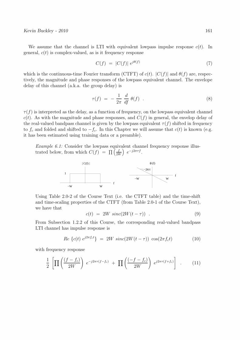
Kevin Buckley - 2010 161
We assume that the channel is LTI with equivalent lowpass impulse response c(t). Ingeneral, c(t) is complex-valued, as is it frequency response
C(f) = |C(f)| ejθ(f) (7)
which is the continuous-time Fourier transform (CTFT) of c(t). |C(f)| and θ(f) are, respec-tively, the magnitude and phase responses of the lowpass equivalent channel. The envelopedelay of this channel (a.k.a. the group delay) is
τ(f) = −1
2π
d
dfθ(f) . (8)
τ(f) is interpreted as the delay, as a function of frequency, on the lowpass equivalent channelc(t). As with the magnitude and phase responses, and C(f) in general, the envelop delay ofthe real-valued bandpass channel is given by the lowpass equivalent τ(f) shifted in frequencyto fc and folded and shifted to −fc. In this Chapter we will assume that c(t) is known (e.g.it has been estimated using training data or a preamble).
Example 6.1: Consider the lowpass equivalent channel frequency response illus-trated below, from which C(f) =
∏
(
f2W
)
e−j2πτf .
θ (f)
−2π τ
| C(f) |
f−W W
1
W−Wf
Using Table 2.0-2 of the Course Text (i.e. the CTFT table) and the time-shiftand time-scaling properties of the CTFT (from Table 2.0-1 of the Course Text),we have that
c(t) = 2W sinc(2W (t − τ)) . (9)
From Subsection 1.2.2 of this Course, the corresponding real-valued bandpassLTI channel has impulse response is
Re c(t) ej2πfct = 2W sinc(2W (t − τ)) cos(2πfct) (10)
with frequency response
1
2
[
∏
(
(f − fc)
2W
)
e−j2πτ(f−fc) +∏
(
(−f − fc)
2W
)
ej2πτ(f+fc)
]
. (11)

Kevin Buckley - 2010 162
The equivalent lowpass noise, z(t), is AWGN and in general complex-valued (unless v(t)and thus c(t) are real-valued). The lowpass equivalent received signal is
rl(t) = v(t) ∗ c(t) + z(t) (12)
=∑
n
In h(t − nT ) + z(t)
whereh(t) = g(t) ∗ c(t) (13)
is the pulse shape at the channel output. Figure 66(b) shows this compact representation.The lowpass equivalent of the symbol observations at the channel output are of the formIm h(t) = sml(t) ∗ c(t); m = 1, 2, · · · , M – i.e. they are distorted. In processing thereceived signal, r(t), both noise and channel distortion should be accounted for.
For a channel without memory, i.e. for c(t) = δ(t), we are back to the situation consideredin Sections 3 & 4 of this Course. That is,
rl(t) =∑
n
In g(t− nT ) + z(t) . (14)
Then, assuming that there is no memory in the modulation process (e.g. no differentialencoding or PRS) and g(t) is restricted to the temporal range 0 ≤ t ≤ T , we can performsymbol-by-symbol detection on rl(t) as described in Section 3 of the Course. With memoryin the modulation process, we can perform MLSE using the Viterbi algorithm as describedin Section 4.
In general the channel has memory resulting, for example, from multipath propagation.This memory result in an overlap of the individual transmitted symbol waveforms (i.e. theIng(t− nT )) at the receiver. That is, as shown in Figure 67 the pulse shape at the receiver,h(t) = g(t)∗c(t), will extend in time beyond the channel input symbol width T , creating ISI.This poses two problems: 1) the symbols, as observed at the receiver, overlap in time; and2) unless c(t) is known, h(t) is unknown as are the symbol observations and basis functionsfor them. The first problem, which we address in this Section, is solved using MLSE (orsymbol-by-symbol MAP). We discuss the second problem later on.
I h(t)0
4I h(t−4T)
nI h(t−nT)n
T 2T 3T 4T t
1
2
3I h(t−T)
I h(t−2T)
I h(t−3T)
Figure 67: The lowpass equivalent channel output is the superposition of the individualsymbol outputs – i.e. the Inh(t − nT ).

Kevin Buckley - 2010 163
In our discussion on symbol detection for an N dimensional modulation scheme, we showedthat;
1. the N matched filters “span” the symbols; and
2. the noise not represented in rn is statistically independent of the noise in rn .
Thus the practice, for the single symbol detection problem, of processing rn instead of rl(t)to detect In seemed justified. Below, in Subsection 6.3, within the more general context ofISI channels, we show formally that the sequence rn is a sufficient statistic for estimatingthe symbols In.
Kevin Buckley - 2010 164
6.2 Signal Design and Partial Response Signaling (PRS) for Ban-dlimited Channels
This discussion corresponds to Subsections 9.2-1, 9.2-2 and 9.2-4 of the Course Text.
ISI at the Receiver Front End Output
Consider the transmission of symbols In; n = 0, 1, 2, · · · ,∞. The lowpass equivalentchannel output is
rl(t) =∞∑
n=0
In h(t − nT ) + z(t) (15)
whereh(t) =
∫ ∞
−∞g(τ) c(t − τ) dτ (16)
is the pulse shape at the channel output (i.e. the convolution of the lowpass equivalentpulse shape into the channel, g(t), and the lowpass equivalent impulse response, c(t), ofthe LTI channel). Assume that at the receiver a filter matched to the received pulse shapeh(t) is applied prior to symbol-rate sampling and subsequent symbol detection or sequenceestimation1. Assume that the matched filter impulse response is2 h∗(−t). The matched filteroutput is then
y(t) = rl(t) ∗ h∗(−t) ∗∞∑
n=0
In x(t − nT ) + v(t) , (17)
wherex(t) = h(t) ∗ h∗(−t) (18)
is the pulse shape at the matched filter output, and v(t) = z(t) ∗ h∗(−t) is the noise.Consider sampling this matched filter output at the symbol rate 1
Tto form
yk = y(kT + τ0) =∞∑
n=0
In x(kT − nT + τ0) + v(kT + τ0) (19)
=∞∑
n=0
In xk−n + vk (20)
where τ0 represent a bulk channel delay3 not represented by the channel impulse responsec(t), xk = x(kT + τ0) and vk = v(kT + τ0). Eq(20) suggest a DT model of an ISI channel.This model is illustrated in Figure 68.
If we assume 4 that x0 = 1, then we have that
yk = Ik +∞∑
n=0; n 6=k
In xk−n + vk , (21)
1The justification for using a matched filter, or equivalently a correlator, at the receiver front end was
presented earlier in Section 3.1 of this Course.2In practice, the matched filter impulse response would be delayed so as to be causal.3With symbol timing recovery, we can assume that this bulk delay is τo = 0.4This implies, for example, that AGC is implemented at the receiver.

Kevin Buckley - 2010 165
c(t)modulator h (−t)*
−1z −1z −1z−1z
(a)
(b)
v(t)
h(t)=g(t)*c(t)
z(t)
y(t) yr (t)l
I k
kT
k
......
v
I I I I
xx0
y
0k k−1
k
k
k+1I
x−2
n+2
......k−1x
B k
Figure 68: (a) An ISI digital communication channel (lowpass equivalent shown); (b) anequivalent discrete-time model.
where the second term on the right side of Eq(21) (i.e. the summation) is the ISI term.So ISI depends on the channel impulse response c(t) through x(t), the pulse shape at thematched filter output.
Consider eye patterns which are described and illustrated on pp. 603-4 of the Course Text.
Signal Design to Eliminate ISI for a Bandlimited Channel
Assume that τ0 = 0. From Eq(21), to avoid ISI we require that
xk = x(kT ) =
1 k = 00 k 6= 0
. (22)
Equivalently, we require that the DTFT of xk be X(ej2πfT ) = 1 for all f . From samplingtheory, we know that the DTFT of xk is related to the CTFT of x(t) as5
X(ej2πfT ) =1
T
∞∑
m=−∞
X(f + m/T ) . (23)
(In terms of the Course Text notation, B(f) =∑∞
m=−∞ X(f + m/T ) = T X(ej2πfT ).) Insummary, in terms of the frequency characteristics of the pulse at the matched filter output,we have
X(ej2πfT ) =1
T
∞∑
m=−∞
X(f + m/T ) = 1 (24)
as our requirement to avoid ISI.
5Refer to the proof on pp. 605-6 of the Course Text.
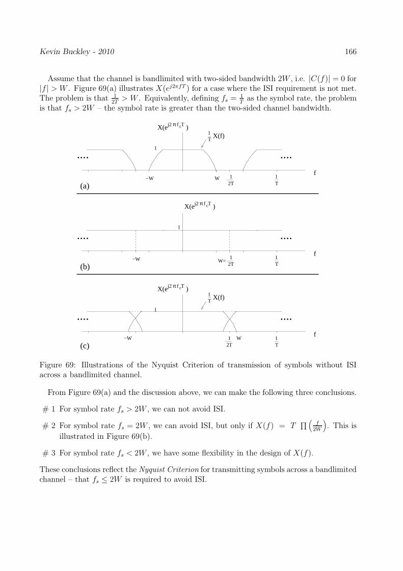
Kevin Buckley - 2010 166
Assume that the channel is bandlimited with two-sided bandwidth 2W , i.e. |C(f)| = 0 for|f | > W . Figure 69(a) illustrates X(ej2πfT ) for a case where the ISI requirement is not met.The problem is that 1
2T> W . Equivalently, defining fs = 1
Tas the symbol rate, the problem
is that fs > 2W – the symbol rate is greater than the two-sided channel bandwidth.
T1
1T
....
2T1
2T1
T1
2T1
T1
1T
....
f
1
X(f)
....
−W W
f
1
W=−W
.... ....
(a)
(b)
(c)
W−Wf
1
X(f)
....
πj2 fX(e )
πj2 fX(e )
πj2 fX(e )
Tc
Tc
Tc
Figure 69: Illustrations of the Nyquist Criterion of transmission of symbols without ISIacross a bandlimited channel.
From Figure 69(a) and the discussion above, we can make the following three conclusions.
# 1 For symbol rate fs > 2W , we can not avoid ISI.
# 2 For symbol rate fs = 2W , we can avoid ISI, but only if X(f) = T∏
(
f2W
)
. This is
illustrated in Figure 69(b).
# 3 For symbol rate fs < 2W , we have some flexibility in the design of X(f).
These conclusions reflect the Nyquist Criterion for transmitting symbols across a bandlimitedchannel – that fs ≤ 2W is required to avoid ISI.
Kevin Buckley - 2010 167
As noted above, for fs = 1T
= 2W we require X(f) = T∏
(
f2W
)
, or equivalently,
x(t) = 2WT sinc(2Wt) , (25)
where, as defined on p. 17 of the Course Text, sinc(x) = sin(πx)πx
. We have no choice in thedesign of x(t), and xk = x(kT ) samples x(t) at all the zero-crossings of the sinc function.One problem with this occurs when there is error in the symbol timing recovery. Then xk
does not sample the sinc function exactly at its zero-crossings, resulting in ISI. The amountof ISI is dictated by the shape of the sinc functions, which has successive peaks that roll-offas t increases at a rate of 1
t.
As noted above, for fs < 2W , we have flexibility in the design of x(t) to meet the require-ment that
∞∑
m=−∞
X(f + m/T ) = T . (26)
This flexibility is used to design x(t) such that it has the zero-crossings att = kT ; k = ±1,±2, · · · required to avoid ISI, while having a roll-off that is faster than 1
tso
as to be less sensitive to symbol timing recovery error. A popular example of such an X(f)is the raised cosine spectrum described on p. 607 of the Course Text, i.e.
Xrc(f) =
T 0 ≤ 0 ≤ |f | ≤ 1−β2T
T2
1 + cos[
πTβ
(
|f | − 1−β2T
)]
1−β2T
≤ |f | ≤ 1+β2T
0 |f | ≥ 1+β2T
, (27)
for 0 ≤ β ≤ 1.If we assume that the channel has lowpass equivalent frequency response C(f) =
∏
( f2W
),then x(t) = g(t) ∗ g(−t) and X(f) = |G(f)|2. So we can avoid ISI directly by design ofthe transmitted pulse shape g(t). For example, to achieve a raised cosine frequency shaping,
G(f) =√
Xrc(f) e−j2πfto (28)
where t0 controls the position in time of g(t).For a general bandlimited channel, with C(f) = 0; |f | > W , recall that
X(f) = H(f) H∗(f) = G(f) C(f) C∗(f)G∗(f) . (29)
One way to design X(f), say as X(f) = Xrc(f), is to require
G(f) =
√
Xrc(f)
C(f)(30)
so that H(f) =√
Xrc(f). Of course, this requires knowledge of C(f) and the design ofa pulse shaping filter at the transmitted that depends on the channel frequency responseC(f). An alternative design is described in Subsection 9.2-4 of the Course Text.

Kevin Buckley - 2010 168
Partial -Response Signaling (PRS) to Control ISI
Consider the ISI model developed above, as described by Eq(20) and illustrated in Figure68. If we relax the no ISI requirement, Eq(22), in a controlled manner, we can shape thematched filter output pulse and spectrum. For example, we may reduce sensitivity to symboltiming recovery error, or shape the spectrum to match that of the channel (e.g. so we donot transmit power in frequency bands nulled by the channel). In Subsection 9.2-2 of theCourse Text, several PRS examples are described. A pulse designed such that
xk = x(kT ) =
1 k = 0, 10 otherwise
(31)
is referred to as a duobinary signal pulse. The
xk = x(kT ) =
1 k = −1−1 k = 10 otherwise
(32)
case is called the modified duobinary signal pulse. The modified duobinary signal pulseCTFT is zero at DC, which is advantageous for channels with a DC null.
Concerning the ISI model illustrated in Figure 68, assume the model is a causal FiniteImpulse Response (FIR) filter on length N , so xk 6= 0 for k = 0, 1, · · · , N − 1 only, i.e.
Bk =N−1∑
n=0
xn Ik−n . (33)
Referring back to Subsection 2.5.2, this is the PRS structure introduced as an approach toshaping the spectrum of the transmitted communication signal. In Section 2.6 we observedhow PRS can be used to shape this spectrum. In Section 4.3 we showed how to implementMLSE for PRS. So now we see that the PRS structure discussed earlier in the Course isactually a model for signal design and control of ISI for symbol transmission at the Nyquistrate fs = 2W . Alternatively, the PRS structure considered earlier in the course can be usedto implement signal design.

Kevin Buckley - 2010 169
6.3 A Discrete-Time ISI Channel Model
This corresponds to Section 9.3 of the Course Text. Following the notation in that Section,we will again use rl(t) to denote the lowpass equivalent of the received signal.
MLSE Formulation with ISI
Let us consider the ML estimation formulation based directly on the lowpass equivalentrl(t). To do this, consider the complete orthonormal expansion of rl(t) in terms of someinfinite set of basis functions6 φk(t); −∞ ≤ t ≤ ∞; k = 1, 2, · · · ,∞. Let
rk =< rl(t), φk(t) > =∫ ∞
−∞rl(t) φ∗
k(t) dt . (34)
Then, under reasonable assumptions on rl(t),
E
|r(t) −∞∑
k=1
rk φk(t)|2
= 0 . (35)
In Figure 70 we illustrate this orthonormal expansion representation of r(t), where the coef-ficient vector r is infinite dimensional.
r
r 1
*
*
.......
.......
2
1 (t)
(t)
φ
φ
lr (t)
( . ) dtr 2
( . ) dt
Figure 70: Orthogonal expansion of the lowpass equivalent received signal rl(t).
To derive an expression for r in terms of the symbol and noise components, we have that
rk =∫ ∞
−∞
(
∑
n
Inh(t − nT ) + z(t)
)
φ∗k(t) dt (36)
=∑
n
In
∫ ∞
−∞h(t − nT ) φ∗
k(t) dt +∫ ∞
−∞z(t) φ∗
k(t) dt
=∑
n
In hkn + zk .
(Note that zk = < z(t), φk(t) > and hkn = < h(t−nT ), φk(t) >.) zk is zero-mean complexGaussian noise with PDF
p(zk) =1
2πN0e−|zk|
2/2N0 , (37)
6Note the these are not the madulation scheme basis fnctions that define the signal space representation.
Kevin Buckley - 2010 170
where N0 is the spectral level of passband n(t) so that σ2z = 2 N0. So, rk is complex Gaussian
with variance σ2z and mean equal to
∑
n In hkn. Note that the zk are mutually uncorrelatedand therefore statistically independent.
Although r is infinite dimensional, it is comprised on discrete components (the rk’s), sowe can describe its joint PDF. To do this, let rN = [r1, r2, · · · , rN ]T , and let I be the infinitedimensional vector of symbols In. The joint PDF of rN is:
p(rN/I) =1
(2πN0)Ne−∑N
k=1|rk−
∑
nInhkn|
2/2N0 . (38)
Let vI(t) =∑
n In h(t−nT ) be the noiseless lowpass equivalent received signal conditionedon I. Then, by Parseval’s Theorem, the power
∑Nk=1 |rk −
∑
n Inhkn|2 is the power of the
representation error rl(t) − vI(t). So,
lnp(r/I) = limN→∞
lnp(rN/I).= −
1
2N0
∫ ∞
−∞|rl(t) − vI(t)|
2 dt . (39)
Consider the power metric
PM(I) = −∫ ∞
−∞|rl(t) − vI(t)|
2 dt (40)
= −∑
k
|rk −∑
n
Inhkn|2 .
Then the equivalent MLSE problem is:
maxI
PM(I) . (41)
The point here is that we do not need to process, directly, all of rl(t) to compute the MLestimate of the symbol sequence In. This is apparent from Eq. (40). The problem hereis that generating and processing the rk is not realistic since producing each rk requires andcontinuous-time inner product over infinite time and there are an infinite number of rk’s.
To overcome this problem, consider Eq. (40):
PM(I) = −∫ ∞
−∞|rl(t) −
∑
n
Inh(t − nT )|2 dt (42)
= −∫ ∞
−∞|rl(t)|
2 dt + 2Re
[
∑
n
I∗n
∫ ∞
−∞rl(t)h
∗(t − nT ) dt
]
−∑
n
∑
m
I∗nIm
∫ ∞
−∞h∗(t − nT )h(t − mT ) dt .
Letyn =
∫ ∞
−∞rl(t) h∗(t − nT ) dt (43)
andxn =
∫ ∞
−∞h∗(t) h(t + nT ) dt . (44)
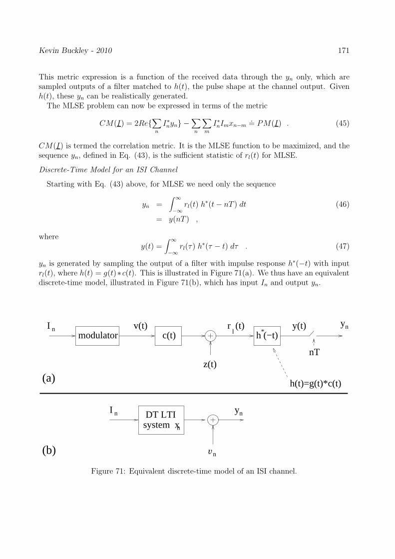
Kevin Buckley - 2010 171
This metric expression is a function of the received data through the yn only, which aresampled outputs of a filter matched to h(t), the pulse shape at the channel output. Givenh(t), these yn can be realistically generated.
The MLSE problem can now be expressed in terms of the metric
CM(I) = 2Re∑
n
I∗nyn −
∑
n
∑
m
I∗nImxn−m
.= PM(I) . (45)
CM(I) is termed the correlation metric. It is the MLSE function to be maximized, and thesequence yn, defined in Eq. (43), is the sufficient statistic of rl(t) for MLSE.
Discrete-Time Model for an ISI Channel
Starting with Eq. (43) above, for MLSE we need only the sequence
yn =∫ ∞
−∞rl(t) h∗(t − nT ) dt (46)
= y(nT ) ,
wherey(t) =
∫ ∞
−∞rl(τ) h∗(τ − t) dτ . (47)
yn is generated by sampling the output of a filter with impulse response h∗(−t) with inputrl(t), where h(t) = g(t)∗c(t). This is illustrated in Figure 71(a). We thus have an equivalentdiscrete-time model, illustrated in Figure 71(b), which has input In and output yn.
c(t)modulatorI n
h (−t)*r (t)
lynv(t)
h(t)=g(t)*c(t)
z(t)
y(t)
nT
system xnDT LTII n yn
nv
(a)
(b)
Figure 71: Equivalent discrete-time model of an ISI channel.

Kevin Buckley - 2010 172
To characterize this equivalent discrete-time channel, note that
yn =∫ ∞
−∞
(
∑
m
Imh(τ − mT ) + z(τ)
)
h∗(τ − nT ) dτ (48)
=∑
m
Im
∫ ∞
−∞h(τ − mT )h∗(τ − nT ) dτ +
∫ ∞
−∞z(τ)h∗(τ − nT ) dτ
=∑
m
Imxn−m + vn
= In ∗ xn + vn ,
wherexn =
∫ ∞
−∞h∗(t) h(t + nT ) dt = h∗(t) ∗ h(−t) |t=nT (49)
are the coefficients of the equivalent discrete-time channel model. Note that x−n = x∗N , i.e.
the equivalent discrete-time channel model has a complex symmetric impulse response. Theadditive noise,
vn =∫ ∞
−∞z(τ)h∗(τ − nT ) dτ , (50)
is Gaussian but not white since it is a sampling of the noise at the output to the receiverfilter h∗(−t).
So, yn can be thought of as being generated as the information sequence In through a DTfilter xn superimposed with the Gaussian noise sequence vn.
Recall that h(t) = g(t) ∗ c(t), where g(t) is the pulse shape into the channel and c(t) is thechannel impulse response. h(t) is the pulse shape at the channel output. If g(t) and c(t) arefinite duration, which they typically are, then so is h(t) and thus xn will be finite durational.This corresponds to a finite memory (i.e. FIR) ISI channel. the channel impulse response isdepicted in Figure 72(a), where for illustration purposes xn is shown as real-valued. Figure72(b) shows the DT channel model. It is a noncausal model, because of the h∗(−t) matchedfilter. In practice, the matched filter would be causal, as would be the DT model.
Noise Whitening at the DT Channel Output
The problem with the DT model developed to this point is that the noise is not white.To see this, consider yn, which is the sampled output of the receiver filter h∗(−t) which ismatched to the modulation pulse at the channel output. Consider the noise component ofit, vn, which is the sampled output of the matched filter h∗(−t) due to the white noise z(t).The autocorrelation function of vn is
Rvv[k] = Ev∗nvn−k (51)
= E∫ ∞
−∞
∫ ∞
−∞z∗(τ1)h(τ1 − nT )z(τ2)h
∗(τ2 − (n + k)T ) dτ1dτ2
=∫ ∞
−∞
∫ ∞
−∞Ez∗(τ1)z(τ2)h(τ1 − nT )h∗(τ2 − (n + k)T ) dτ1dτ2
=∫ ∞
−∞
∫ ∞
−∞2N0δ(τ1 − τ2)h(τ1 − nT )h∗(τ2 − (n + k)T ) dτ1dτ2
= 2 N0
∫ ∞
−∞h(t − nT )h∗(t − (n + k)T ) dt
= 2 N0 xk .
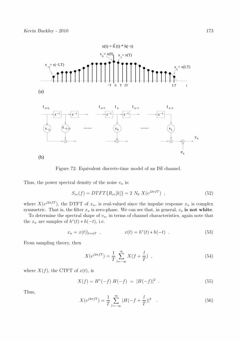
Kevin Buckley - 2010 173
*x(t) = h (t) * h(−t)
x = x(LT)L
−Lx = x(−LT)
x = x(T)10
x = x(0)
−1z −1z −1z −1z −1z
x−Lx−L+1 x0 xL
yn
n+LI n+1I nI n−1I n−LI
−T 0 T 2T LT t
...... ......
(b)
(a)
nv
Figure 72: Equivalent discrete-time model of an ISI channel.
Thus, the power spectral density of the noise vn is:
Svv(f) = DTFTRvv[k] = 2 N0 X(ej2πfT ) , (52)
where X(ej2πfT ), the DTFT of xn, is real-valued since the impulse response xn is complexsymmetric. That is, the filter xn is zero-phase. We can see that, in general, vn is not white.
To determine the spectral shape of vn, in terms of channel characteristics, again note thatthe xn are samples of h∗(t) ∗ h(−t), i.e.
xn = x(t)|t=nT , x(t) = h∗(t) ∗ h(−t) . (53)
From sampling theory, then
X(ej2πfT ) =1
T
∞∑
l=−∞
X(f +l
T) , (54)
where X(f), the CTFT of x(t), is
X(f) = H∗(−f) H(−f) = |H(−f)|2 . (55)
Thus,
X(ej2πfT ) =1
T
∞∑
l=−∞
|H(−f +l
T)|2 . (56)

Kevin Buckley - 2010 174
Depending on subsequent processing, whitening of vn may or may not be necessary. Forexample, efficient application of the Viterbi algorithm for MLSE requires that the noisebe white, while the white-noise assumption is not critical for channel equalizers. Here weconsider whitening vn.
Figure 73 shows the processing of yn to whiten its noise component vn. A(z) denotes thewhitening filter transfer function, vn the output, and ηn the white noise component of theoutput. A(ej2πfT ) = A(z)|z=ej2πfT is the whitening filter frequency response.
yn
vn nη
vnWhitening Filter
A(z)
Figure 73: Whitening of the sampled matched filter output noise vn.
Since Svv(f) = 2 N0 X(ej2πfT ) and Sηη(f) = Svv(f) |A(ej2πfT )|2, to whiten ηn we requirethat
X(ej2πfT ) |A(ej2πfT )|2 = 1 (57)
so that Sηη(f) = 2 N0 = σ2η. Let X(z) =
∑Ln=−L xn z−n be the transfer function of the
DT filter model xn. To realize Eq (57) consider factoring X(z) as
X(z) = F (z) F ∗(z−1) . (58)
If such a factorization can be found then, since
F ∗(ej2πfT ) = F ∗(z−1)∣
∣
∣
z=ej2πfT, (59)
we can write
X(ej2πfT ) = F (ej2πfT ) F ∗(ej2πfT ) = F (z) F ∗(z−1)∣
∣
∣
z=ej2πfT, (60)
in which case
A(z) =1
F ∗(z−1)(61)
will provide the desired whitening, since
A(ej2πfT ) =1
F ∗(ej2πfT )(62)
and thus
|A(ej2πfT )|2 =1
F ∗(ej2πfT ) F (ej2πfT )=
1
|X(ej2πfT )|2. (63)

Kevin Buckley - 2010 175
To see how X(z) can be factored as in Eq (58), recall that xn is complex symmetric. Thismeans7 that for every zero zk of the FIR filter transfer functionX(z) =
∑Ln=−L xnz−n, there is a zero z−1
k . This zero configuration is illustrated in Figure 74for a real-valued xn (so that zeros occur in complex conjugate pairs).
z−1k
( )*
*zk
z−1k
zk
z−plane
Figure 74: Zero configuration for the symmetric noncausal DT channel model.
If we let
F (z) =L∏
k=1
(z − zk) , (64)
i.e. with zeros at zk; k = 1, 2, · · · , L, then
F ∗(z−1) =L∏
k=1
(z−1 − zk)∗ (65)
will have zeros at z = 1zk
. Thus X(z) can be factored as in Eq (58), where for each pair of
X(z) zeros, zk,1zk, one is assigned to F (z) and the other will be for F ∗(z−1). There are 2L
choices for these zero assignments, corresponding to 2L choices for the whitening filter A(z).For one of these choices, F (z) will be causal.
Figure 75(a) illustrates the whitening filter A(z) applied to the DT ISI channel modelidentified to this point. Figure 75(b,c) show the new DT ISI channel which incorporates theDT whitening filter. The impulse response fn; n = 0, 1, · · · , L for this DT ISI channel modelis obtained as follows:
1. Identify h(t) = g(t) ∗ c(t).
2. Determine X(ej2πfT ) = 1T
∑∞l=−∞ |H(−f + l
T)|2, and thus X(z).
3. Factor X(z) as X(z) = F (z) F ∗(z−1) (i.e. assign the X(z) zeros to F (z) as indicatedabove).
4. Derive fn as the inverse z-transform of F (z).
7See Oppenheim and Schafer, Discrete-Time Signal Processing, Prentice-Hall, 1989, p. 265.

Kevin Buckley - 2010 176
Note that c(t), the channel impulse response, is assumed known. In Section 7 of this Coursewe address the problem of unknown c(t).
The noise at the whitening filter output, ηn, is zero-mean AWGN with variance σ2η = 2 N0.
F (z )* −1A(z) = 1
vn
vn
f 0 f 1 f L
z−1 z−1 z−1I n
vn
η n
.....
I n
F(z)vn
η n
I n
(a)
ny
(b)
(c)
X(z) = F(z) F (z )−1*
Figure 75: DT ISI channel model including noise whitening.

Kevin Buckley - 2010 177
6.4 MLSE and the Viterbi Algorithm for ISI Channels
This Section of the Course corresponds to Subsection 9.3-3 of the Course Text.In Section 6.3 of the Course Notes, directly above, we established the equivalent discrete-
time lowpass channel representation of an ISI communication channel which is applicablefor modulation schemes for which the equivalent lowpass transmitted signal is of the form
v(t) =∑
n
In g(t− nT ) . (66)
This representation is reproduced below in Figure 76. The output is8
vn = fT In,L + ηn (67)
where f = [f0, f1, · · · , fL]T , In,L = [In, In−1, · · · , In−L]T , ηn is discrete-time, complex-valued
AWGN with variance σ2η = 2N0, and fH f =
∑Lk=0 |fk|
2 = 1.
f 0 f 1 f L
z−1 z−1 z−1I n
vn
η n
present inputsymbol
.....
I In−1 n−L
past input symbols
Figure 76: DT ISI channel model including noise whitening.
8Note that the notation for this whitening filter output, vn, should not be confused with that of the
sampled matched filter output noise, vn.

Kevin Buckley - 2010 178
Since we know that the sequence vn forms a sufficient statistic for MLSE of the sequenceIn, we can formulate this MLSE problem, at time n, in terms of the joint PDF ofvn = [v1, v2, · · · , vn]
T conditioned on In = [I1, I2, · · · , In]T :
p(vn/In) =1
(πσ2η)
ne−∑n
k=1|vk−fT Ik,L|2/σ2
η . (68)
Concerning notation, here we represent current time (i.e. the most recent symbol time thatwe want to optimuze up to) as n, and k represents all symbol time up to n. We then considerincrementing to the next current time n + 1.
The MLSE problem, at symbol time n, is
maxIn
p(vn/In) . (69)
Taking the negative natural log and eliminating constant terms that do not effect the relativecosts for different In’s, we have the equivalent problem9
minIn
Λn(In) = −PM(In) =n∑
k=1
|vk − fT Ik,L|2 , (70)
where Λn(In) is the cost of sequence In. The first n − 1 elements of In are equal to In−1,i.e. In[1 : n − 1] = In−1. This suggests that at time n we may be able to time-recursivelyextend time n − 1 results.
The Viterbi algorithm efficiently solves this MLSE problem time-recursively (i.e. as nincreases). Let
Λn(In) =n∑
k=1
|vk − fT Ik,L|2 (71)
=n∑
k=1
λ(Ik,L)
= Λn−1(In−1) + λ(In,L) .
The term λ(Ik,L) = |vk − fT Ik,L|2 is the incremental cost of a symbol sequence In in going
from time k − 1 to time k.
9In Chapters 4 & 9 of the Course Text, where MLSE and the Viterbi algorithm are discussed, several
notations are used to represent the measure or metric to be optimized. When PM is used, it is maximized,
and typically refers to a probability metric. When CM is used, it is minimized, and is sometimes referred to
as a correlation of cross-correlation metric. CM is related to but not equal to a Euclidean distance. Here,
I start using the notation Λ and refer to it as a cost to be mimimized. As used here, it is close to but not
the same as CM of Subsection 9.3-1 of the Course Text. Here it is a Euclidean distance. I choose Λ so as to
get away from the variety of Course Text notations, and because I’ve used this notation in other places to
represent cost. This is the cost used in subsequent Viterbi algorithm examples, and in the Viterbi algorithm
Matlab code provided for Computer Assignment 2.

Kevin Buckley - 2010 179
At time n−1 there would be Mn−1 of these costs, one for each sequence In−1. Given thesecosts at time n − 1, the Mn costs at time n (i.e. the cost of the possible sequences In) canbe easily computed by extending the Λn−1(In−1) as in Eq. (71). Thus, each Λn−(In−1) isextended by all λ(In,L) consistent with Λn−1(In−1). Also note that, although there appearsto be Mn incremental costs λ(In,L) required to extend the costs at time n−1 to those at timen, there are at most only ML+1 unique incremental costs, since these costs are determined byIn,L, of which there are ML+1 possible values, intead of by the set of Mn possible sequencesIn from time 1 up to time n. This is what leads to the optimality of the Viterbi algorithm.
As with its application to MLSE and MAP sequence estimation for modulation schemeswith memory, the idea behind the Viterbi algorithm is to, at time n,
1. keep only the Λn−1(In−1) needed to compute the Λn(In) corresponding to possibleoptimum In (i.e. eliminate or prune the In that can not possibly be optimum); and
2. use the Λn−1(In−1) and the λ(In,L) to compute the needed Λn(In).
Paralleling its development for modulation schemes with memory, we again do this by rep-resenting the Λn(In) as paths of a trellis diagram. Since all paths into a trellis state will beextended using the same incremental costs (i.e. incremental costs for time n are computedusing only: 1) the symbols represented by the previous state and, 2) the new values yn
and In), only the lowest cost path into each state need be considered). Thus, the Viterbialgorithm to prune the paths.
Consider the DT channel model shown in Figure 76. Define the “state” as the set ofoutputs of the L delays. For the L elements of the state, and M possible values at eachelement, there are ML possible states. The trellis maps the ML possible states at any time tothe ML possible states at the next time. Associated with this mapping are costs associatedwith going from one state value to the next.
Next we use a couple of examples to illustrate how the trellis represents symbol sequencesand their costs, and how the Viterbi algorithm can be used to reduce the computational costof finding the MLSE solution.
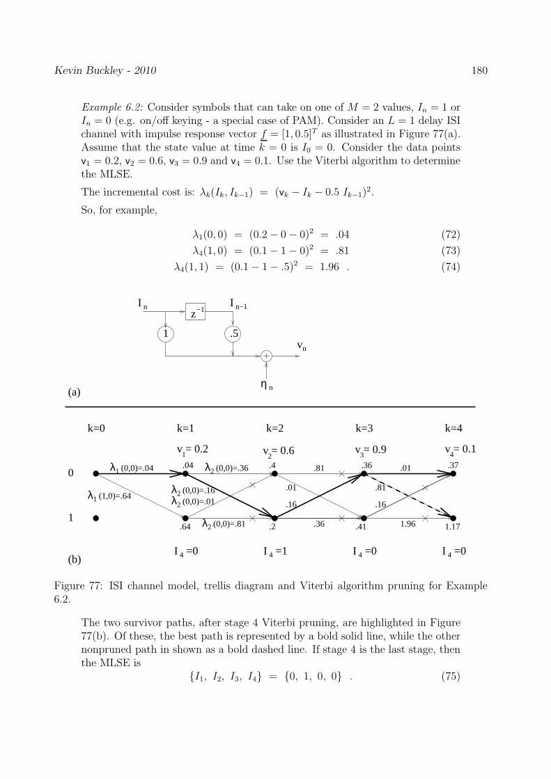
Kevin Buckley - 2010 180
Example 6.2: Consider symbols that can take on one of M = 2 values, In = 1 orIn = 0 (e.g. on/off keying - a special case of PAM). Consider an L = 1 delay ISIchannel with impulse response vector f = [1, 0.5]T as illustrated in Figure 77(a).Assume that the state value at time k = 0 is I0 = 0. Consider the data pointsv1 = 0.2, v2 = 0.6, v3 = 0.9 and v4 = 0.1. Use the Viterbi algorithm to determinethe MLSE.
The incremental cost is: λk(Ik, Ik−1) = (vk − Ik − 0.5 Ik−1)2.
So, for example,
λ1(0, 0) = (0.2 − 0 − 0)2 = .04 (72)
λ4(1, 0) = (0.1 − 1 − 0)2 = .81 (73)
λ4(1, 1) = (0.1 − 1 − .5)2 = 1.96 . (74)
(0,0)=.04λ1
λ1 (1,0)=.64
λ2 (0,0)=.36
λ2λ2 (0,0)=.01
λ2 (0,0)=.81
4I =0 4I =1 4I =0 4I =0
1 4
k=0 k=1 k=2 k=3 k=4
v = 0.22 3v = 0.6 v = 0.9 v = 0.1
0.04
.64
.4
.2
.36
.41
.37
1.17
(0,0)=.16
.81
.36
.01
.16
.81
.01
.16
1.961
z−1
vn
I n I n−1
1 .5
nη
(b)
(a)
Figure 77: ISI channel model, trellis diagram and Viterbi algorithm pruning for Example6.2.
The two survivor paths, after stage 4 Viterbi pruning, are highlighted in Figure77(b). Of these, the best path is represented by a bold solid line, while the othernonpruned path in shown as a bold dashed line. If stage 4 is the last stage, thenthe MLSE is
I1, I2, I3, I4 = 0, 1, 0, 0 . (75)
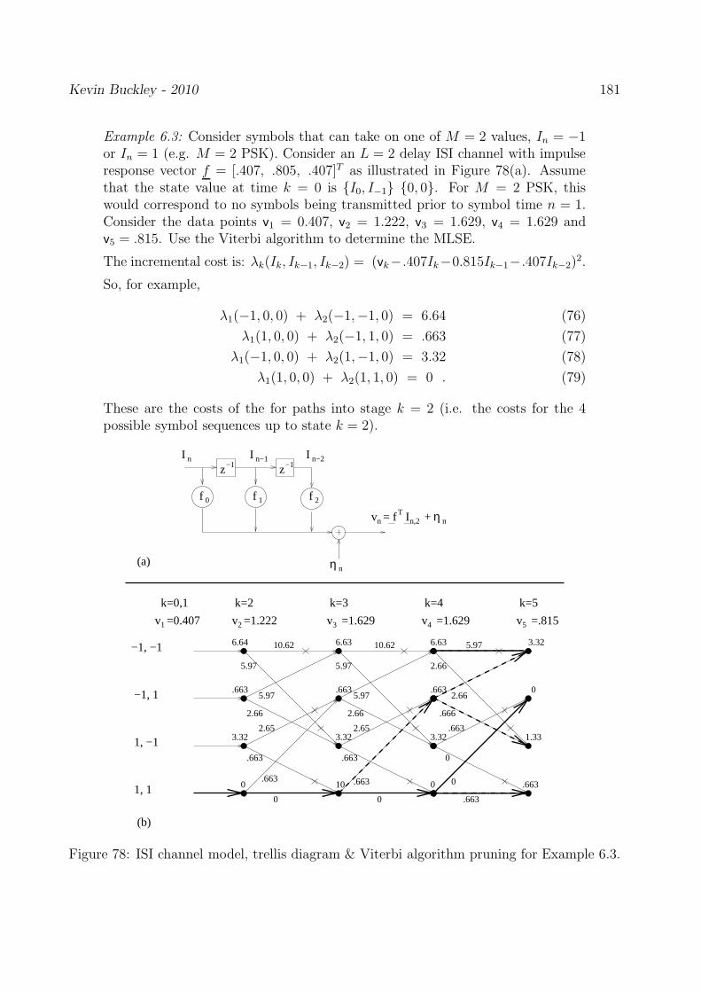
Kevin Buckley - 2010 181
Example 6.3: Consider symbols that can take on one of M = 2 values, In = −1or In = 1 (e.g. M = 2 PSK). Consider an L = 2 delay ISI channel with impulseresponse vector f = [.407, .805, .407]T as illustrated in Figure 78(a). Assumethat the state value at time k = 0 is I0, I−1 0, 0. For M = 2 PSK, thiswould correspond to no symbols being transmitted prior to symbol time n = 1.Consider the data points v1 = 0.407, v2 = 1.222, v3 = 1.629, v4 = 1.629 andv5 = .815. Use the Viterbi algorithm to determine the MLSE.
The incremental cost is: λk(Ik, Ik−1, Ik−2) = (vk−.407Ik−0.815Ik−1−.407Ik−2)2.
So, for example,
λ1(−1, 0, 0) + λ2(−1,−1, 0) = 6.64 (76)
λ1(1, 0, 0) + λ2(−1, 1, 0) = .663 (77)
λ1(−1, 0, 0) + λ2(1,−1, 0) = 3.32 (78)
λ1(1, 0, 0) + λ2(1, 1, 0) = 0 . (79)
These are the costs of the for paths into stage k = 2 (i.e. the costs for the 4possible symbol sequences up to state k = 2).
z−1z−1
f 0 f 1 f 2
η n
I n−2n−1II n
v =1.2222
(a)
(b)
nv = f I +n,2
−1, −1
1, 1
1, −1
−1, 1
k=0,1
10
k=2 k=3 k=4 k=5
v =1.629 v =1.6293 4 5v =.815
.663
6.64
0
6.63
.663
3.32
6.63
.663
3.32
0
10.62
5.97
5.97
2.66
.663
0
3.32
.663
10.62
0
.663
.663
2.66
5.97
5.97
2.652.65
.663
0
0
.663
.666
2.66
5.97
2.66
.663
1.33
0
3.32
1v =0.407
T η n
Figure 78: ISI channel model, trellis diagram & Viterbi algorithm pruning for Example 6.3.

Kevin Buckley - 2010 182
Figure 78(b) shows the trellis diagram and Viterbi pruning through stage 5.After pruning at stage 5, the 4 survivor parts (one into each state) have costs3.32, 0, 1.33, .663. These paths highlighted. The one corresponding to thelowest cost at stage 5 is the one that is completely solid. It corresponds to symbolsequence I1 = 1, I2 = 1, I3 = 1, I4 = 1, I5 = −1. This would be the MLSEif stage 5 was the last.
With a path cost of zero, it is tempting to conclude that there is no channelnoise, since the received data is exactly the data that would be realized ifI1 = 1, I2 = 1, I3 = 1, I4 = 1, I5 = −1 were actually transmitted.
Finally note that, even if more data is to come, we can say difinitively that theevential MLSE will have I1 = 1, I2 = 1, I3 = 1.
Practical Issues
Trellis Truncation: (See Proakis: p. 246, first paragraph; p. 513, 1-st paragraph.)
In general, given vn; n = 1, 2, · · · , K, the MLSE of IK can not be determined for any n untilall data up to n = K is processed. For continuous, on-line symbol estimation, i.e. K = ∞,and even for large finite K, this can be impractical. In practice, at any time n the trellisis “truncated” q samples into the past. That is, at each symbol time n, the best survivorpath into stage n is traced back q stage, to stage n − q. The value of In−q corresponding tothat path is taken as the estimate. Note that this In−q estimate is not guaranteed to be theeventual MLSE. However if all paths at stage n have merged back at stage n − q, then In−q
will be the MLSE.A useful rule of thumb, which has been shown empirically to result in negligible perfor-
mance loss, is q ≥ 5L where L is the memory depth of the modulation scheme plus channel.
A Numerical Issue:
For continuous symbol estimation, the numerical value of the minumum cost path toeach state grows without bound as time progresses. In practice this probem is resolved byperiodically (say at every P th stage) subtracting the smallest path cost from all path costs.
Unknown Channel Coefficients:
The implementation of MLSE and the Viterbi algorithm for ISI channels, as describedabove, requires knowledge of the ISI channel coefficients. That is, the coefficient vector f ofthe equivalent discrete-time model is needed to compute the trellis branch costs. This vectoris a function of the actual channel impulse response c(t).
In many applications this channel information is not known prior to processing. In thesecases the channel coefficients must be either estimated along with the symbols or otherwisedealt with. This issue will be overviewed later, in Section 7.6 of the Course.

Kevin Buckley - 2010 181
ECE8700Communication Systems Engineering
Villanova UniversityECE Department
Prof. Kevin M. Buckley
Lecture 11
−3 −2 −1 0 1 2 3−20
−10
0
10(a) channel
ω (rad/sample)
Fre
q. R
sp. (
dB)
−3 −2 −1 0 1 2 3
0
10
20
30
(b) equalizer
ω (rad/sample)
Fre
q. R
sp. (
dB)
−3 −2 −1 0 1 2 3−20
−10
0
(c) channel/equalizer
ω (rad/sample)
Fre
q. R
sp. (
dB)
0 5 10 15 20 25 30 35 40−0.5
0
0.5
1(d) channel/equalizer
k
f * c
opt
−2 0 2−2
−1.5
−1
−0.5
0
0.5
1
1.5
2
Re Ik
Im I k
−2 0 2−2
−1.5
−1
−0.5
0
0.5
1
1.5
2
Re vk
Im v k
−2 0 2−2
−1.5
−1
−0.5
0
0.5
1
1.5
2
Re Ihatk
Im Ih
at k

Kevin Buckley - 2010 182
Contents
7 Channel Equalization 1837.1 Basic Concepts . . . . . . . . . . . . . . . . . . . . . . . . . . . . . . . . . . 1837.2 Linear Equalization . . . . . . . . . . . . . . . . . . . . . . . . . . . . . . . . 186
7.2.1 Channel Inversion . . . . . . . . . . . . . . . . . . . . . . . . . . . . . 1867.2.2 Mean Squared Error (MSE) Criterion . . . . . . . . . . . . . . . . . . 1887.2.3 Additional Linear MMSE Equalizer Issues . . . . . . . . . . . . . . . 198
List of Figures
79 Two DT ISI model and corresponding equalizers. . . . . . . . . . . . . . . . 18480 The DT ISI channel model after whitening. . . . . . . . . . . . . . . . . . . . 18581 Channel inverse equalizers. . . . . . . . . . . . . . . . . . . . . . . . . . . . . 18782 Noncausal and causal linear time invariance channel equalizers. . . . . . . . . 18983 Channel/equalizer characteristics for Example 7.1. . . . . . . . . . . . . . . . 19284 Scatter plots for Example 7.1. . . . . . . . . . . . . . . . . . . . . . . . . . . 19285 Channel/equalizer characteristics for Example 7.2. . . . . . . . . . . . . . . . 19386 Scatter plots for Example 7.2. . . . . . . . . . . . . . . . . . . . . . . . . . . 19387 Channel/equalizer characteristics for Example 7.3. . . . . . . . . . . . . . . . 19588 Scatter plots for Example 7.3. . . . . . . . . . . . . . . . . . . . . . . . . . . 19589 Channel/equalizer characteristics for Example 7.4. . . . . . . . . . . . . . . . 19690 Channel/equalizer characteristics for Example 7.5. . . . . . . . . . . . . . . . 19791 Scatter plots for Example 7.5. . . . . . . . . . . . . . . . . . . . . . . . . . . 19792 P = 2 cut oversampling and associated DT ISI channel model. . . . . . . . . 20193 P = 2 cut fractionally spaced linear equalizer. . . . . . . . . . . . . . . . . . 202

Kevin Buckley - 2010 183
7 Channel Equalization
This Chapter of the Course corresponds to Sections 9.4 & 9.5 of the Course Text.As in the last Chapter of these Course Notes, here we address the problem of channel
induced ISI. Again, we assume a linear channel, however we now take a very different ap-proach. Instead of sequence estimation, we will first try to compensate for (or equalize) theeffect of the channel using a receiver filtr (called an equalizer), and we will then performdetection of individual symbols.
7.1 Basic Concepts
Following are several important points concerning the channel equalization approach to mit-igating ISI:
1. the channel equalizer will process a discrete-time receiver signal, i.e. the sampledoutput of a matched filter.
2. Some channel equalization algorithms are developed ignoring additive noise. Suchalgorithm tend to perform worse than algorithms which account for noise, especiallywhen the channel has nulls in its frequency response.
3. The two basic equalizer structures considered here are: 1) the linear equalizer structure;and 2) the Decision Feedback Equalizer (DFE) structure.
4. There are two basic modes for the design and implementation of either linear equalizersor DFEs: 1) the training mode (based on transmitted training symbols that are knownat the receiver); and 2) the decision directed mode (for previous detected symbolsreplace training symbols at the receiver).
5. The processing will not be optimal with respect to the symbol detection or sequenceestimation criteria that we have considered previously (e.g. ML or MAP). Equaliz-ers will be designed using optimum filtering formulations (e.g. channel inversion orminimum mean squared error (MMSE) filter design).
6. Optimum equalizer filter design algorithms require knowledge of the channel impulseresponse. This shortcoming can be effectively elleviated using and adaptive filteringalgorithm which will self-design the equalizer so as to approximate the optimum equal-izer.
These issues will be addressed in this Chapter of the Course.

Kevin Buckley - 2010 184
Figure 79 is an illustration of the discrete-time channel model developed previously. Anequalizer, with transfer function C(z), is applied to the channel output of the whitening filter
1F ∗(z−1)
. Alternatively, the whitening filter can be eliminated and the equalizer C′
(z) can beapplied directly to the sampler output yk. Recall that we represent the equivalent discrete-time ISI channel model, before whitening, with impulse response xk or equivalently transferfunction X(z). We also represent the discrete-time ISI channel model, after whitening, withimpulse response fk or transfer function F (z). In both cases the output of the equalizer isdenoted Ik since it is an estimate of the symbol sequence Ik.
There are two fundamentally different approaches to ISI channel equalization:
1. Channel Inversion, where C(z) = 1F (z)
or C′
(z) = 1X(z)
is the ideal objective, and theideal output is
Ik = Ik + nk (1)
where nk is additive noise; and
2. Minimization of mean squared error (MSE), where
minC(z)
E|Ik − Ik|2 , (2)
or some similar optimization problem is solved.
The channel inversion approach will assure the elimination of ISI. However, for a channel withspectral nulls over some frequency band, an equalizer designed based on channel inversion willhave large gain over that frequency band, and thus will have the disadvantage of significantamplification of any noise in that frequency band. With the MMSE design approach, thereis no guarantee that the signal at the equalizer output will not be distorted (i.e. there maybe some residual ISI), but there will be an optimum tradeoff (in the MSE sense) betweensignal distortion and additive noise suppression.
The transfer function notation C(z) and C′
(z) implies that the equalizer is linear and timeinvariant. However, we will additionally consider nonlinear decision feedback equalizers andtime-varying data adaptive equalizers.
X(z)−1*
F (z )−1vkI k
I k
I k
kv
C(z)
C ’ (z)
or
F(z)
Figure 79: Two DT ISI model and corresponding equalizers.
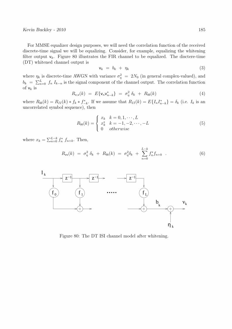
Kevin Buckley - 2010 185
For MMSE equalizer design purposes, we will need the correlation function of the receiveddiscrete-time signal we will be equalizing. Consider, for example, equalizing the whiteningfilter output vk. Figure 80 illustrates the FIR channel to be equalized. The disctere-time(DT) whitened channel output is
vk = bk + ηk (3)
where ηk is discrete-time AWGN with variance σ2η = 2N0 (in general complex-valued), and
bk =∑L
n=0 fn Ik−n is the signal component of the channel output. The correlation functionof vk is
Rv,v(k) = Evnv
∗
n−k = σ2η δk + Rbb(k) (4)
where Rbb(k) = RII(k) ∗ fk ∗ f ∗
−k. If we assume that RII(k) = EInI∗
n−k = δk (i.e. Ik is anuncorrelated symbol sequence), then
Rbb(k) =
xk k = 0, 1, · · · , Lx∗
k k = −1,−2, · · · ,−L0 otherwise
(5)
where xk =∑L−k
n=0 f ∗
n fn+k. Then,
Rvv
(k) = σ2η δk + Rbb(k) = σ2
ηδk +L−k∑
n=0
f ∗
nfn+k . (6)
f 0 f 1 f L
z−1 z−1 z−1
.....v
η
I k
k
kkb
Figure 80: The DT ISI channel model after whitening.

Kevin Buckley - 2010 186
7.2 Linear Equalization
In this Section we will consider channel inversion based design of a linear time-invariant(LTI) equalizer C(z). The design of C
′
(z) would proceed in a similar manner. We considerboth an FIR filter structure and an unrestricted LTI structure.
7.2.1 Channel Inversion
Channel inversion equalization is also referred to a zero-crossing equalization and peak dis-tortion criterion based equalization.
Figure 81(a) shows the general equalizer problem. Let
qk = ck ∗ fk =∞∑
j=−∞
cj fk−j . (7)
Then
Ik = Ik ∗ qk =∞∑
j=−∞
Ij qk−j = q0 Ik + · · · (8)
The zero-crossing design objective is
qk = δk ; all k , (9)
orck ∗ fk = δk . (10)
Taking the z-transform, we have
C(z)F (z) = 1 or C(z) =1
F (z). (11)
This is the channel inverse equalizer. Figure 81(b) illustrates this equalizer. (The channelinverse equalizer for the DT channel model without whitening C
′
(z) is shown in Figure81(c)).Previously we have shown that the noise before the whitening filter, i.e. vk, has powerspectral density
Svv(f) = 2N0 X(ej2πfT ) |f | ≤1
2T, (12)
the noise power spectral density of the equalizer output noise is then
Snn(f) = |C′
(ej2πfT )|2 Svv(f) (13)
=1
X(ej2πfT ) X∗(ej2πfT )2N0 X(ej2πfT )
=2N0
X(ej2πfT )
since X(ej2πfT ) is real-valued (i.e. xk is complex symmetric). Recall that
X(ej2πfT ) =1
T
∞∑
l=−∞
|H(f + l1
T)|2 . (14)

Kevin Buckley - 2010 187
I k vk I kC(z)
kη
F(z)
I k vk
kη
I k
I k I k
kv
yX(z) X (z)
−1
F (z)−1
Q(z)
F(z)
k
(a)
(b)
(c)
Figure 81: Channel inverse equalizers.
X(ej2πfT ) can have spectral nulls if H(f) has. If this is the case, then Snn(f) will have largegains at some frequencies, and the noise power,
σ2n =
∫ 1/2T
−1/2TSnn(f) df (15)
can be very large. Noise amplification is the major limitation of channel inversion equaliza-tion.
The above discussion assumes no restriction on C(z). Often, the equalizer will be restrictedto be FIR, i.e.
C(z) = c−KzK + c−K+1zK−1 + · · · + c0 + c1z
−1 + · · ·+ cKz−K , (16)
(see p. 649 of the Course Text) with corresponding output,
Ik =K∑
j=−K
cjvk−j . (17)
In general, a channel F (z) or X(z) can not be prefectly inverted with an FIR equalizer. Thisis because the channel is FIR, and an FIR system can not be inverted with an FIR system(i.e. only poles can exactly cancel zeros, and FIR transfer function can not invert an FIRtransfer function).
In practice, this noncausal FIR filter can be realized by designating the current output ofthe whitening filter as vk+K.

Kevin Buckley - 2010 188
7.2.2 Mean Squared Error (MSE) Criterion
Consider the DT linear time invariant channel models established in Section 3 of the Course.This model has as its input the symbol sequence Ik. It output could be, for example: 1)the sampled output of the receiver demodulator; or 2) the sampled output, denoted yk, ofthe receiver filter matched to the pulse shape h(t) at the channel output; or 3) the output,denoted vk, of the DT filter which noise-whitens the sampled matched filter output yk. Asan example we will consider processing vk.
Here we consider a DT linear time invariant equalizer with input vk, transfer functionC(z), impulse response ck, and output sequence Ik which is to be considered an estimateof the symbol sequence Ik. Note that Ik is implicitly a function of the equalizer transferfunction C(z), or equivalently the equalizer impulse response ck. Consider, as equalizerdesign objective, the MSE cost function
J = E|Ik − Ik|2 . (18)
The Minimum MMSE (MMSE) equalizer is the solution to the problem
minC(z)
J . (19)
That is , the design problem is to select C(z) (or equivalently ck) to minimize the cost J .
FIR C(z)
First consider an equalizer which has a structure which is constrained to be FIR. Theformulation for this in the Course Text, shown here in Figure 82(a), is noncausal. K is theFIR equalizer memory depth design parameter. The MMSE will decrease as K increases.However, increasing K increases computational requirements, and as we will see, for adaptiveequalizers increasing K can actually lead to increased MSE.
The formulation we will use is shown in Figure 82(b). It is a causal FIR equalizer of lengthK1 + 1 and latency (delay) ∆. K1 and ∆ are design parameters. In terms of the noncausalequalizer design parameter K, reasonable values for K1 and ∆ are K1 = 2K and ∆. If thechannel has some bulk propagation delay, say of B symbols, then ∆ > B is desirable. Forexample, ∆ = B + K1
2is reasonable.
The output of the causal FIR equalizer is
Ik−∆ = ck ∗ vk =K1∑
j=0
cjvk−j = cTvk (20)
where vk = [vk, vk−1, · · · , vk−K1]T and c = [c0, c1, · · · , cK1
]T is the FIR equalizer coefficientvector. Define the error as
ek−∆ = Ik−∆ − cTvk , (21)
which is a linear function of the coefficient vector c. Consider the cost
J = J(c/K1, ∆) = E|ek−∆|2 , (22)

Kevin Buckley - 2010 189
z−1 z−1 z−1
vk vk−1 vk−K1
0c 1c cK 1K
I k−∆
.....
z−1
I k
z−1 z−1z−1 z−1
c−Kc−K+1 c0
(b)
(a)
v vk−K
.....
vvk+K−1k+K k
..... cKK
Figure 82: Noncausal and causal linear time invariance channel equalizers.
where the notation J(c/K1, ∆) explicitly shows that the cost is a function of c and it dependson given values of K1 and ∆. We have that
J(c/K1, ∆) = E|Ik−∆ − cTvk|
2 (23)
= E|Ik−∆|2 − EcT
vk I∗
k−∆ − EIk−∆ vHk c∗ + EcT
vk vHk c∗
= σ2I − cT ζ∗ − ζT c∗ + cT Υ∗ c∗
where ζ = EIk−∆ v∗
k is the cross correlation vector between Ik−∆ and vk and Υ = Ev∗k vTk
is the covariance matrix of vk.Note that since Υ is the correlation matrix of vk, it is symmetric and positive definite. If
vk is complex-valued, assumed above, then Υ is complex symmetric.
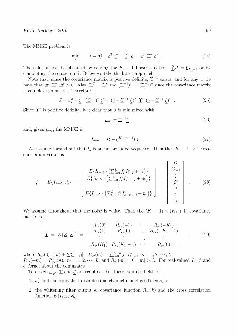
Kevin Buckley - 2010 190
The MMSE problem is
minc
J = σ2I − cT ζ∗ − ζT c∗ + cT Υ∗ c∗ . (24)
The solution can be obtained by solving the K1 + 1 linear equations ∂∂c
J = 0K1+1 or bycompleting the square on J . Below we take the latter approach.
Note that, since the covariance matrix is positive definite, Υ−1 exists, and for any w wehave that wT Υ∗ w∗ > 0. Also, ΥT = Υ∗ and (Υ−1)T = (Υ−1)∗ since the covariance matrixis complex symmetric. Therefore
J = σ2I − ζT (Υ−1)∗ ζ∗ + (c − Υ−1 ζ)T Υ∗ (c − Υ−1 ζ)∗ . (25)
Since Υ∗ is positive definite, it is clear that J is minimized with
copt = Υ−1ζ (26)
and, given copt, the MMSE is
Jmin = σ2I − ζH (Υ−1) ζ . (27)
We assume throughout that Ik is an uncorrelated sequence. Then the (K1 + 1) × 1 crosscorrelation vector is
ζ = EIk−∆ v∗
k =
EIk−∆ ·(
∑Ll=0 f ∗
l I∗
k−l + ηk
)
EIk−∆ ·(
∑Ll=0 f ∗
l I∗
k−1−l + ηk
)
...
EIk−∆ ·(
∑Ll=0 f ∗
l I∗
k−K1−l + ηk
)
=
f ∗
∆
f ∗
∆−1...
f ∗
0
0...0
. (28)
We assume throughout that the noise is white. Then the (K1 + 1) × (K1 + 1) covariancematrix is
Υ = Ev∗k vTk =
Rvv
(0) Rvv
(−1) · · · Rvv
(−K1)R
vv(1) R
vv(0) · · · R
vv(−K1 + 1)
......
. . ....
Rvv
(K1) Rvv
(K1 − 1) · · · Rvv
(0)
, (29)
where Rvv
(0) = σ2η +
∑Ll=0 |fl|
2, Rvv
(m) =∑L−m
l=0 fl f ∗
l+m; m = 1, 2, · · · , L,R
vv(−m) = R∗
vv(m); m = 1, 2, · · · , L, and R
vv(m) = 0; |m| > L. For real-valued Ik, f and
c, forget about the conjugates.To design copt, Υ and ζ are required. For these, you need either:
1. σ2n and the equivalent discrete-time channel model coefficients; or
2. the whitening filter output vk covariance function Rvv
(k) and the cross correlationfunction EIk−∆ v
∗
k.
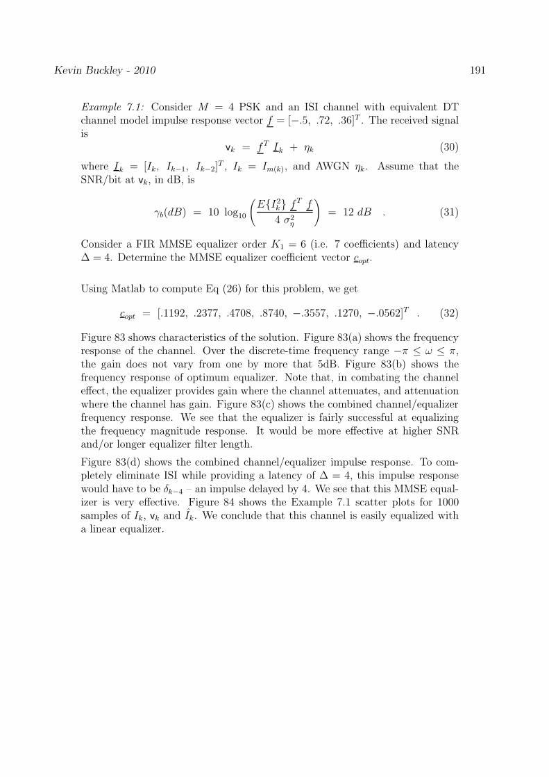
Kevin Buckley - 2010 191
Example 7.1: Consider M = 4 PSK and an ISI channel with equivalent DTchannel model impulse response vector f = [−.5, .72, .36]T . The received signalis
vk = fT Ik + ηk (30)
where Ik = [Ik, Ik−1, Ik−2]T , Ik = Im(k), and AWGN ηk. Assume that the
SNR/bit at vk, in dB, is
γb(dB) = 10 log10
(
EI2k fT f
4 σ2η
)
= 12 dB . (31)
Consider a FIR MMSE equalizer order K1 = 6 (i.e. 7 coefficients) and latency∆ = 4. Determine the MMSE equalizer coefficient vector copt.
Using Matlab to compute Eq (26) for this problem, we get
copt = [.1192, .2377, .4708, .8740, −.3557, .1270, −.0562]T . (32)
Figure 83 shows characteristics of the solution. Figure 83(a) shows the frequencyresponse of the channel. Over the discrete-time frequency range −π ≤ ω ≤ π,the gain does not vary from one by more that 5dB. Figure 83(b) shows thefrequency response of optimum equalizer. Note that, in combating the channeleffect, the equalizer provides gain where the channel attenuates, and attenuationwhere the channel has gain. Figure 83(c) shows the combined channel/equalizerfrequency response. We see that the equalizer is fairly successful at equalizingthe frequency magnitude response. It would be more effective at higher SNRand/or longer equalizer filter length.
Figure 83(d) shows the combined channel/equalizer impulse response. To com-pletely eliminate ISI while providing a latency of ∆ = 4, this impulse responsewould have to be δk−4 – an impulse delayed by 4. We see that this MMSE equal-izer is very effective. Figure 84 shows the Example 7.1 scatter plots for 1000samples of Ik, vk and Ik. We conclude that this channel is easily equalized witha linear equalizer.
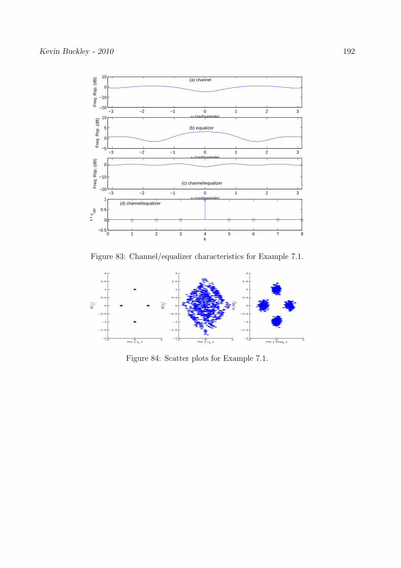
Kevin Buckley - 2010 192
−3 −2 −1 0 1 2 3−20
−10
0
10(a) channel
ω (rad/sample)
Fre
q. R
sp. (
dB)
−3 −2 −1 0 1 2 3−5
0
5
10
(b) equalizer
ω (rad/sample)
Fre
q. R
sp. (
dB)
−3 −2 −1 0 1 2 3−20
−10
0
(c) channel/equalizer
ω (rad/sample)
Fre
q. R
sp. (
dB)
0 1 2 3 4 5 6 7 8−0.5
0
0.5
1(d) channel/equalizer
k
f * c
opt
Figure 83: Channel/equalizer characteristics for Example 7.1.
−2 0 2−2
−1.5
−1
−0.5
0
0.5
1
1.5
2
Re Ik
Im I k
−2 0 2−2
−1.5
−1
−0.5
0
0.5
1
1.5
2
Re vk
Im v k
−2 0 2−2
−1.5
−1
−0.5
0
0.5
1
1.5
2
Re Ihatk
Im Ih
at k
Figure 84: Scatter plots for Example 7.1.

Kevin Buckley - 2010 193
Example 7.2: the same as Example 7.1, except that f = [.8, −.6]T , γb = 9 dB,K1 = 16 and ∆ = 9.
Figure 85 shows characteristics of the solution.
−3 −2 −1 0 1 2 3−20
−10
0
10(a) channel
ω (rad/sample)
Fre
q. R
sp. (
dB)
−3 −2 −1 0 1 2 3−5
0
5
10
(b) equalizer
ω (rad/sample)
Fre
q. R
sp. (
dB)
−3 −2 −1 0 1 2 3−20
−10
0
(c) channel/equalizer
ω (rad/sample)
Fre
q. R
sp. (
dB)
0 2 4 6 8 10 12 14 16 18−0.5
0
0.5
1(d) channel/equalizer
k
f * c
opt
Figure 85: Channel/equalizer characteristics for Example 7.2.
Results are somewhat similar to those in Example 7.1. The primary differenceis that the channel now has a moderate null at DC, as shown in Figure 85(a).Figures 85(b,c) show that the equalizer is not very successful at equalizing thechannel attenuation at low frequencies, even though, compared to Example 7.1,a longer equalizer filter was used.
Figure 85(d) shows that there will be some residual ISI after equalization. Figure86 shows the Example 7.2 scatter plots for 1000 samples of Ik, vk and Ik. Weconclude that a linear equalizer can be somewhat effective with this channel, butthat the moderate null does limit performance.
−2 0 2−2
−1.5
−1
−0.5
0
0.5
1
1.5
2
Re Ik
Im I k
−2 0 2−2
−1.5
−1
−0.5
0
0.5
1
1.5
2
Re vk
Im v k
−2 0 2−2
−1.5
−1
−0.5
0
0.5
1
1.5
2
Re Ihatk
Im Ih
at k
Figure 86: Scatter plots for Example 7.2.

Kevin Buckley - 2010 194
Example 7.3: Again consider M = 4 PSK and an ISI channel, this time withequivalent DT channel model impulse response vector f = [.407, .815, .407]T .Again let γb = 12 dB. Consider a FIR MMSE equalizer order K1 = 6 andlatency ∆ = 4.
Using Matlab to compute Eq (26) for this problem, we get
copt = [−.0083, .1816, −.6766, 1.6342, −.6766, .1816, −.0083]T . (33)
Figure 87 shows characteristics of the solution. Figure 87(a) shows the frequencyresponse of the channel. Notice the high frequency null, which makes this chan-nel difficult to equalize with a linear filter. Figure 87(b) shows the frequencyresponse of optimum equalizer. Note that, in combating the channel effect, theequalizer “tries” to provide gain at higher frequencies. The filter is successfulin the mid frequency range. However, at the highest frequencies, inverting thechannel frequency response would require substantial gain. Since, at 12dB, thenoise level is not insignificant, the equalizer can not provide this gain withoutsignificant amplification of the noise. Thus, the optimum equalizer shuts off athigh frequency. Figure 87(c) shows the combined channel/equalizer frequencyresponse. Note that, with gain close to 0dB, equalization is effective at lowerfrequencies where the channel attenuation is not too significant. However, theMMSE linear equalizer can not provide the gain around ω = ±π required toinvert the channel.
Figure 87(d) shows the combined channel/equalizer impulse response. To com-pletely eliminate ISI while providing a latency of ∆ = 4, this impulse responsewould have to be δk−4 – an impulse delayed by 4. Instead, we see significant ISI.Combining the frequency response and impulse response results, we can see theISI/noise-gain tradeoff characteristic of the linear MMSE equalizer.
Figure 88 shows the Example 7.3 scatter plots for 1000 samples of Ik, vk and Ik.We conclude that, because of the deep spectral null, the MMSE linear equalizerfails to equalize this channel.

Kevin Buckley - 2010 195
−3 −2 −1 0 1 2 3−20
−10
0
10(a) channel
ω (rad/sample)
Fre
q. R
sp. (
dB)
−3 −2 −1 0 1 2 3−5
0
5
10
(b) equalizer
ω (rad/sample)
Fre
q. R
sp. (
dB)
−3 −2 −1 0 1 2 3−20
−10
0
(c) channel/equalizer
ω (rad/sample)
Fre
q. R
sp. (
dB)
0 1 2 3 4 5 6 7 8−0.5
0
0.5
1(d) channel/equalizer
k
f * c
opt
Figure 87: Channel/equalizer characteristics for Example 7.3.
−2 0 2−2
−1.5
−1
−0.5
0
0.5
1
1.5
2
Re Ik
Im I k
−2 0 2−2
−1.5
−1
−0.5
0
0.5
1
1.5
2
Re vk
Im v k
−2 0 2−2
−1.5
−1
−0.5
0
0.5
1
1.5
2
Re Ihatk
Im Ih
at k
Figure 88: Scatter plots for Example 7.3.
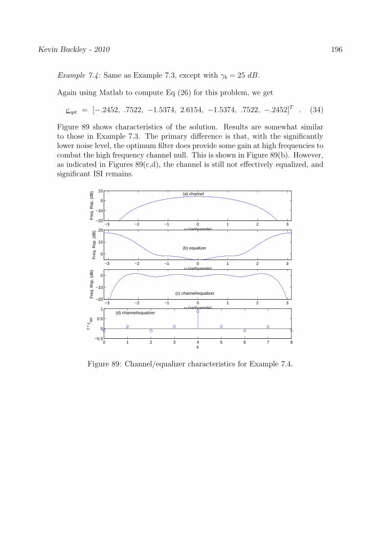
Kevin Buckley - 2010 196
Example 7.4: Same as Example 7.3, except with γb = 25 dB.
Again using Matlab to compute Eq (26) for this problem, we get
copt = [−.2452, .7522, −1.5374, 2.6154, −1.5374, .7522, −.2452]T . (34)
Figure 89 shows characteristics of the solution. Results are somewhat similarto those in Example 7.3. The primary difference is that, with the significantlylower noise level, the optimum filter does provide some gain at high frequencies tocombat the high frequency channel null. This is shown in Figure 89(b). However,as indicated in Figures 89(c,d), the channel is still not effectively equalized, andsignificant ISI remains.
−3 −2 −1 0 1 2 3−20
−10
0
10(a) channel
ω (rad/sample)
Fre
q. R
sp. (
dB)
−3 −2 −1 0 1 2 3
0
10
20
(b) equalizer
ω (rad/sample)
Fre
q. R
sp. (
dB)
−3 −2 −1 0 1 2 3−20
−10
0
(c) channel/equalizer
ω (rad/sample)
Fre
q. R
sp. (
dB)
0 1 2 3 4 5 6 7 8−0.5
0
0.5
1(d) channel/equalizer
k
f * c
opt
Figure 89: Channel/equalizer characteristics for Example 7.4.

Kevin Buckley - 2010 197
Example 7.5: Same as Example 7.4, except with K1 = 38.
Figure 90 shows characteristics of the solution.
Results are somewhat somewhat better those in Examples 7.3 and 7.4. This time,with the longer FIR equalizer, the equalizer does a very good job of invertingthe channel frequency response except at the higher frequencies very near thechannel spectral null. We can see this by comparing Figures 87(a,b), and byinspection of Figure 89(c). However, Figure 89(d) shows that the channel ispartially equalized, and some ISI remains. Figure ?? shows the Example 7.5scatter plots for Ik, vk and Ik.
We conclude that this channel is not easily equalized with a linear equalizer.Increasing K1 beyond that of Example 7.5 will not improve performance signif-icantly. A linear equalizer of any length can not effectively equalize a channelwith a deep spectral null, regardless of the SNR.
−3 −2 −1 0 1 2 3−20
−10
0
10(a) channel
ω (rad/sample)
Fre
q. R
sp. (
dB)
−3 −2 −1 0 1 2 3
0
10
20
30
(b) equalizer
ω (rad/sample)
Fre
q. R
sp. (
dB)
−3 −2 −1 0 1 2 3−20
−10
0
(c) channel/equalizer
ω (rad/sample)
Fre
q. R
sp. (
dB)
0 5 10 15 20 25 30 35 40−0.5
0
0.5
1(d) channel/equalizer
k
f * c
opt
Figure 90: Channel/equalizer characteristics for Example 7.5.
−2 0 2−2
−1.5
−1
−0.5
0
0.5
1
1.5
2
Re Ik
Im I k
−2 0 2−2
−1.5
−1
−0.5
0
0.5
1
1.5
2
Re vk
Im v k
−2 0 2−2
−1.5
−1
−0.5
0
0.5
1
1.5
2
Re Ihatk
Im Ih
at k
Figure 91: Scatter plots for Example 7.5.
Kevin Buckley - 2010 198
7.2.3 Additional Linear MMSE Equalizer Issues
Unconstrained Linear Equalizer
The formulation of the MSE equalizer discussed above in Subsection 7.2.2 assumes thatthe equalizer is FIR. That is, the equalizer is constrained to have an FIR structure. Theunconstrained MSE equalizer can also be derived. As with the unconstrained channel in-version equalizer, the formulation is in terms of the equalizer transfer function. It is moreenlightening to formulate the unconstrained MSE equalizer problem in terms of the transferfunction C
′
(z) which is applied to the output of the sampler, without any whitening filter.The unconstrained MMSE equalizer is derived on pp. 645-648 of the Course Text. Its
transfer function is
C′
opt(z) =1
X(z) + N0
. (35)
Compared to the unconstrained channel inversion equalizer, for which C′
(z) = 1X(z)
, we seethat with the MMSE equalizer additive white noise is accounted for by the additional N0
term in the transfer function denominator.
For high SNR (i.e. for low noise level N0), the MMSE transfer function approaches
C′
opt(z) =1
X(z). (36)
In this case, the MMSE equalizer inverts the channel. On the other hand, for low SNR (i.e.for high noise level N0), the MMSE transfer function approaches
C′
opt(z) =1
N0
. (37)
The MMSE equalizer transfer function goes to the constant N−10 , which indicates that the
equalizer provides no frequency selective filtering. Instead it basically shuts down. In be-tween these two limiting cases, the MMSE filter optimally trades-off additive white noisesuppression and channel inversion.
From a channel inversion equalizer point of view, the additional additive N0 term in thedenominator of equalizer transfer function acts as a regularization term, controlling the noisegain by limiting the gain in the frequency response C
′
opt(ej2πfT ).
Design of C′
opt(z) requires: 1) knowledge of X(z), which in turn requires knowledge ofthe channel equivalent lowpass impulse response c(t); 2) the assumption that the lowpassequivalent additive channel/receiver noise z(t) is white; and 3) knowledge of the spectrallevel N0 of the additive noise z(t).

Kevin Buckley - 2010 199
Colored Noise and Interference Cancellation
When the additive noise z(t) is not white, for example because the receiver noise is coloredor the receiver picks up interference signals, then C
′
(z) = 1X(z)+N0
is not the optimum MMSEequalizer.
Let Szz(f) be the PSD of the additive channel/receiver noise. It can be shown that theoptimum equalizer has a transfer function of the form
C′
opt(ej2πT ) =
X(ej2πT )
|X(ej2πT )|2 + Svv(f), (38)
where Svv(f), the PSD of the noise vn at the sampler output, is
Svv(f) =1
T
∞∑
l=−∞
Szz(f +l
T) |H(f +
l
T)|2 , (39)
and as before H(f) is the CTFT of the pulse at the channel output.
Comments on MSE Equalizer Performance
Figure 9.4-5 on p. 654 of the Course Text shows the impulse responses of three equivalentdiscrete-time channels for which equalizer performance was studied. The 2-nd channel is onethat you are considering in computer assignments. Figure 9.4-6 shows the correspondingchannel frequency responses. Note that two of the channels have spectral nulls in theirfrequency responses.
For M = 2 symbol antipodal PAM, Figure 9.4-4 compares the performance of the MMSEequalizer for each channel. Symbol error probabilities are shown for the three MMSE equal-ized channels along with the “ideal” performance realized when there is no channel inducedISI.
Note that rather long (K1+1 = 31 tap) equalizers were used for all channels, with ∆ = 16.Even with the large K1, equalizer performance is not good for the two channels that havespectral nulls in their frequency responses. Channel inversion equalizers would perform evenworse for the channels with spectral nulls, since channel inversion would result in significantnoise gain.
These results point to the principal limitation of linear equalizers. Linear equalizers usuallydo not perform well for channels that have spectral nulls in there frequency response.

Kevin Buckley - 2010 200
.

Kevin Buckley - 2010 201
Fractionally Spaced Linear Equalizers
To this point, in using the discrete-time equivalent model of the communication system andISI channel, we have been assuming that the receiver sampler operates at the symbol rate.This sampling rate was justified using a sufficient statistic argument for MMSE. Lookingback at the argument that established the optimality of sampling at this rate, it requiredthat the channel impulse response (explicitly the channel output pulse shape) is known,so that the receiver output can be matched filtered prior to sampling. When the channelimpulse response in unknown, or when the matched filter in not implemented, sampling atthe symbol rate 1
Tmay no longer be adequate for generation of sufficient statistics for MMSE.
Sampling at a higher rate can then result in improved performance.When the channel impulse response c(t) is not known, the receiver filter is commonly
matched to g(t), and equalizers are sometimes operated at a higher sampling rate to improveperformance. The Figure 92(a) depicts this oversampling scheme, where the sample rate is1T
′ with T′
< T . Typically PT′
= T for positive integer P , and we refer to P as the numberof cuts. For example, for P = 2 cuts, Figure 92(a) illustrates the sampling. Figure 92(b)shows the equivalent DT model, where f
i= [fi,0, fi,1, · · · fi,L]T ; i = 1, 2.
η
vf2 2,k
2,k
f1
η
v
1,k
1,k
I k
v2,ko
v1,kx
(a)
(b)
x x x x x x x x oooooooo
0 3T2TT 4T 5T 6T 7T
Figure 92: P = 2 cut oversampling and associated DT ISI channel model.

Kevin Buckley - 2010 202
Consider the P = 2 cut MMSE fractionally spaced linear equalizer illustrated in Fig-ure 93. Assume that Eη∗
1,k η2,j = 0 for all k, j. Let vk = [vT1,k, v
T2,k]
T with vi,k =[vi,k, vi,k−1, · · · , vi,k−K1
]T , and c = [cT1 , cT
2 ]T with ci = [ci,0, ci,1, · · · , ci,K1]T . Then
Ik−∆ = cTvk . (40)
In Homework #7 you are asked to derive the expression for the MMSE coefficient vector copt
for this equalizer.
I k−∆
z−1 z−1 z−1
.....
v v v
1c c c
2,k 2,k−1 2,k−K
2,0 2,1 2,K
1
z−1 z−1 z−1
v1,k
.....
v v1,k−1 1,k−K
1c1,0 c1,1c
1
1,K
Figure 93: P = 2 cut fractionally spaced linear equalizer.
For P > 2 cuts, we simply extend Figure 93, using P FIR filters.
Array Linear Equalizers
Consider receiving a transmitted digital communication signal with P receiver antenna.Assume that the channel from the transmitter to each receiver is an ISI channel. Assumeeach receiver antenna has front-end electronics and a sampler so as to generate a DT signalvi,k; i = 1, 2, · · · , P . Each of these DT signals can be modeled as the output of an equivalentDT model of the channel from the transmitter to its receiver antenna.
We can consider each of these signals as a cut, which leads to a linear equalizer structureand design problem analogous to the fractionally spaced linear equalizer. In Homework #8you are asked to design a P = 2 array linear equalizer.
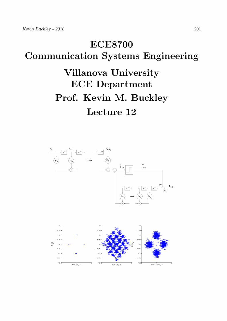
Kevin Buckley - 2010 201
ECE8700
Communication Systems Engineering
Villanova University
ECE Department
Prof. Kevin M. Buckley
Lecture 12
z−1 z−1 z−1
vk vk−1 vk−K1
0c 1c cK 1K
I k−∆
z−1z−1z−1
KKb2 b2 1b....
I k−∆
I k−∆~
.....
(a)
(b)
−2 0 2−2
−1.5
−1
−0.5
0
0.5
1
1.5
2
Re Ik
Im I k
−2 0 2−2
−1.5
−1
−0.5
0
0.5
1
1.5
2
Re vk
−2 0 2−2
−1.5
−1
−0.5
0
0.5
1
1.5
2
Re Ihatk
Im Ih
at k
Kevin Buckley - 2010 202
Contents
7 Channel Equalization 203
7.1 Basic Concepts . . . . . . . . . . . . . . . . . . . . . . . . . . . . . . . . . . 2037.2 Linear Equalization . . . . . . . . . . . . . . . . . . . . . . . . . . . . . . . . 2037.3 Decision Feedback Equalization . . . . . . . . . . . . . . . . . . . . . . . . . 203
List of Figures
94 The Decision Feedback Equalizer (DFE). . . . . . . . . . . . . . . . . . . . . 20395 An equivalent block diagram of the DFE in training mode. . . . . . . . . . . 20596 Channel/equalizer characteristics for Example 7.6. . . . . . . . . . . . . . . . 20797 Scatter plots for Example 7.6. . . . . . . . . . . . . . . . . . . . . . . . . . . 20798 Channel/equalizer characteristics for Example 7.7. . . . . . . . . . . . . . . . 20899 Scatter plots for Example 7.7. . . . . . . . . . . . . . . . . . . . . . . . . . . 208100 P = 2 cut (i.e. fractionally spaced or array) DFE. . . . . . . . . . . . . . . . 209
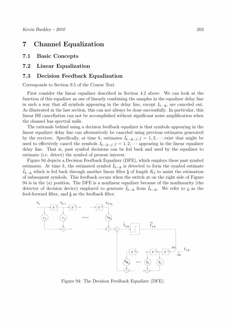
Kevin Buckley - 2010 203
7 Channel Equalization
7.1 Basic Concepts
7.2 Linear Equalization
7.3 Decision Feedback Equalization
Corresponds to Section 9.5 of the Course Text.
First consider the linear equalizer described in Section 4.2 above. We can look at thefunction of this equalizer as one of linearly combining the samples in the equalizer delay linein such a way that all symbols appearing in the delay line, except Ik−∆, are canceled out.As illustrated in the last section, this can not always be done successfully. In particular, thislinear ISI cancellation can not be accomplished without significant noise amplification whenthe channel has spectral nulls.
The rationale behind using a decision feedback equalizer is that symbols appearing in thelinear equalizer delay line can alternatively be canceled using previous estimates generatedby the receiver. Specifically, at time k, estimates Ik−∆−j; j = 1, 2, · · · exist that might beused to effectively cancel the symbols Ik−∆−j; j = 1, 2, · · · appearing in the linear equalizerdelay line. That is, past symbol decisions can be fed back and used by the equalizer toestimate (i.e. detect) the symbol of present interest.
Figure 94 depicts a Decision Feedback Equalizer (DFE), which employs these past symbolestimates. At time k, the estimated symbol Ik−∆ is detected to form the symbol estimateIk−∆ which is fed back through another linear filter b of length K2 to assist the estimationof subsequent symbols. This feedback occurs when the switch at on the right side of Figure94 is in the (a) position. The DFE is a nonlinear equalizer because of the nonlinearity (thedetector of decision device) employed to generate Ik−∆ from Ik−∆. We refer to c as thefeed-forward filter, and b as the feedback filter.
z−1 z−1 z−1
vk vk−1 vk−K1
0c 1c cK 1K
I k−∆
z−1z−1z−1
KKb2 b2 1b....
I k−∆
I k−∆~
.....
(a)
(b)
Figure 94: The Decision Feedback Equalizer (DFE).

Kevin Buckley - 2010 204
The DFE design problem is to determine c and b, the feed-forward and feedback DFEcoefficient vectors. To do this, note that
Ik−∆ =K1∑
j=0
cjvk−j +K2∑
j=1
bj Ik−∆−j (1)
= cTvk + bT Ik−∆−1
wherec = [c0, c1, · · · , cK1
]T , (2)
b = [b1, b2, · · · , bK2]T , (3)
vk = [vk, vk−1, · · · , vk−K1]T , (4)
andIk−∆−1 = [Ik−∆−1, Ik−∆−2, · · · Ik−∆−K2
]T . (5)
To derive a design equation, first consider the error
e1k−∆ = Ik−∆ − Ik−∆ . (6)
The problem with this error is that it is a highly nonlinear function of c and b, since Ik−∆
is a function of Ik−∆−j; j = 1, 2, · · · , K2 which are functions of c and b. Thus, minimizingthe mean squared value of (6) would be very difficult. General closed form expressions ofoptimum c and b do not exist.
Consider the alternative error
e2k−∆ = Ik−∆ − Ik−∆ , (7)
where Ik−∆ is obtained from (1) by replacing the Ik−∆−j with Ik−∆−j. That is,
Ik−∆ =K1∑
j=0
cjvk−j +K2∑
j=1
bjIk−∆−j (8)
= cTvk + bT Ik−∆−1
= wT xk ,
where w = [cT , bT ]T and xk = [vTk , IT
k−∆−1]T . Since Ik−∆−1 is not a function of c and b, e2
k−∆
is a linear function of c and b, and an “optimum” expression for the DFE coefficients canbe derived (optimum in the sense of the mean squared value of e2
k−∆, which is not of directinterest).
Let the cost be
J = J(w/K1, K2, ∆) = E|e2k−∆|
2 = E|Ik−∆ − Ik−∆|2 . (9)
The solution to the problemmin
wJ(w/K1, K2, ∆) (10)

Kevin Buckley - 2010 205
iswopt = R−1r (11)
whereR = Ex∗
kxTk (12)
andr = EIk−∆x∗
k . (13)
As a problem for Homework #8 you are asked to identify R and r in terms of the noisepower σ2
n and the discrete-time channel model coefficients fl; l = 0, 1, · · · , L.
The advantage in formulating the DFE design problem in terms of e2k−∆ instead of e1
k−∆
is that a closed form expression for the equalizer coefficients is realized. The resultingcoefficients do not optimize any actual error (unless the actual symbols Ik−∆ are fed backas opposed to the detected symbols Ik−∆ – which seems impractical). Nonetheless, theperformance of the DFE resulting from design equation (11) can be very good, as long asthe detector is making correct decisions most of the time. This will be the case when bothSNR is high enough and the DFE structure is adequate (e.g. when K1, K2 and ∆ are selectedproperly).
In Figure 94, consider the structure when the switch on the right side is in position (b).For reasons that will become clear when we discuss adaptive equalizers in Section 7.4 below,we call this the training mode configuration as opposed to the decision feedback mode (whenthe switch is in the (a) position). In the training mode, Eq (9) is the actual cost, and Eq(11) is the MMSE DFE coefficient vector. Figure 95 shows an equivalent block diagram.
f c
b
I kI k−∆^
I k−∆
.
−( +1)∆z
η
vk
k
Figure 95: An equivalent block diagram of the DFE in training mode.
The impulse response, from Ik to Ik−∆ is
hk = fk ∗ ck + δk−(∆+1) ∗ bk (14)
where δk is the DT impulse function. The corresponding transfer function is
H(z) = F (z) C(z) + z−(∆+1) B(z) . (15)
Ideal equalization, in training mode, occurs if hk = δk−∆ or equivalently if H(z) = z−∆.

Kevin Buckley - 2010 206
Figure 95 illustrates the principal advantage of the DFE over the linear equalizer. Withthe linear equalizer, only c can be used to invert the effect of f . As we have seen, this cannot be effectively accomplished when the channel f has spectral nulls. On the other hand,with the DFE, c does not have to invert f to achieve good performance. Both c and b areadjusted so as to approximate hk = δk−∆. Specifically note that even if the channel f hasspectral nulls, the desired result can be accomplished since b can provide the required gainat the frequencies f attenuates.
Example 7.6: Consider again the modulation scheme and channel for Examples 7.3-5 – M = 4PSK and f = [.407, .815, .407]T . As with Examples 7.4-5, let γb = 25 dB. Consider aMMSE DFE K1 = 3, K2 = 3 and latency ∆ = 3. Note that a total of 7 coefficients are used,4 feed-forward (in c) and 3 feedback (in b). This is the same number of multipliers used forExamples 3-5. The MMSE DFE coefficient vector is
wopt = [.0376, −.1040, .1904, 2.1694, −1.8456, −.8830, 0]T , (16)
so that
copt = [.0376, −.1040, .1904, 2.1694]T bopt = [−1.8456, −.8830 0]T . (17)
Figure 96 shows characteristics of the solution. Notice the combined impulse response of thechannel and the feed-forward section of the DFE shown in Figure 96(a). Denote this impulseresponse qk = fk ∗ck. As with the linear equalizer, for the feed-forward section to completelyeliminate ISI by itself, we would need qk = δk−∆. The actual qk is close to zero for delay lessthan ∆ = 3, indicating that the feed-forward section does a good job of eliminating ISI fromsymbols future in time to the symbol of interest. Also, with q∆ ≈ 1, the desired symbol ispassed with approximately unit gain. Note however that qk is significant for some k > ∆,indicating that at the output of the feed-forward filter there is significant ISI due to symbolsin the past of the desired signals. This is the ISI that the feedback section of the DFE isdesigned to handle. Figure 96(b) shows the overall impulse response, from IK to Ik−∆ inFigure 95. Denote this impulse response as hk. The feedback filter effects hk for k > ∆ only.In this range, it effectively cancels qk. The fact that hk ≈ δk−∆ indicates that the signalportion of DFE output Ik−∆ should closely approximate Ik−∆. Of course there is still thenoise component of Ik−∆, but the MMSE design criterion works to minimize this.
Note that although hk is not the actual impulse response in decision directed mode, as longas correct decisions are being made most of the time, hk does characterize the actual ISI atthe DFE output. Figure 97 shows scatter plots of Ik, vk and Ik−∆ for the MMSE DFE run intraining mode. It is clear that the DFE is very effective for this challenging channel, whereaswe saw in Examples 7.3-5 that a linear equalizer was not effective, even with a substantiallylarger number of coefficients.

Kevin Buckley - 2010 207
0 0.5 1 1.5 2 2.5 3 3.5 4 4.5 5
0
1
2
(a) channel/feed−forward
k
f k * c
k
0 0.5 1 1.5 2 2.5 3 3.5 4 4.5 5−0.5
0
0.5
1
1.5
(b) channel/feed−forward − feedback
k
f k * c
k + b
k− ∆
−1
−3 −2 −1 0 1 2 3−20
−15
−10
−5
0
5
(c) channel/equalizer
ω (rad/sample)
Fre
q. R
sp. (
dB)
Figure 96: Channel/equalizer characteristics for Example 7.6.
−2 0 2−2
−1.5
−1
−0.5
0
0.5
1
1.5
2
Re Ik
Im I k
−2 0 2−2
−1.5
−1
−0.5
0
0.5
1
1.5
2
Re vk
−2 0 2−2
−1.5
−1
−0.5
0
0.5
1
1.5
2
Re Ihatk
Im Ih
at k
Figure 97: Scatter plots for Example 7.6.
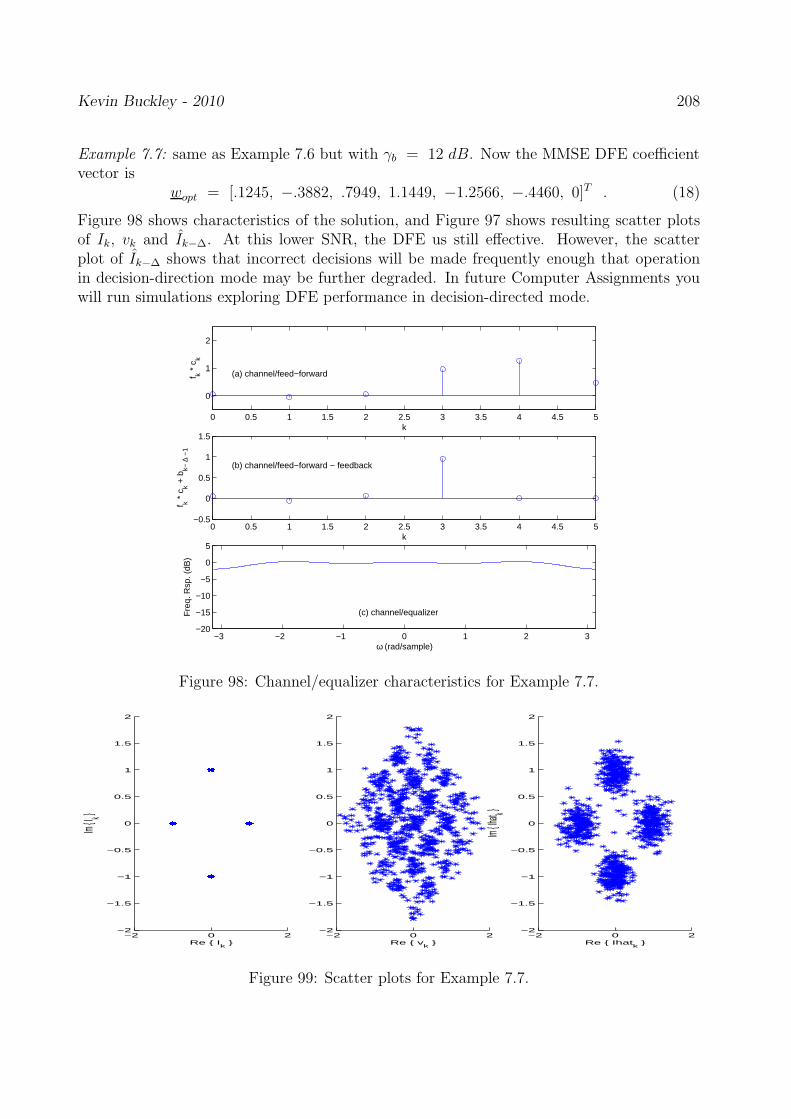
Kevin Buckley - 2010 208
Example 7.7: same as Example 7.6 but with γb = 12 dB. Now the MMSE DFE coefficientvector is
wopt = [.1245, −.3882, .7949, 1.1449, −1.2566, −.4460, 0]T . (18)
Figure 98 shows characteristics of the solution, and Figure 97 shows resulting scatter plotsof Ik, vk and Ik−∆. At this lower SNR, the DFE us still effective. However, the scatterplot of Ik−∆ shows that incorrect decisions will be made frequently enough that operationin decision-direction mode may be further degraded. In future Computer Assignments youwill run simulations exploring DFE performance in decision-directed mode.
0 0.5 1 1.5 2 2.5 3 3.5 4 4.5 5
0
1
2
(a) channel/feed−forward
k
f k * c
k
0 0.5 1 1.5 2 2.5 3 3.5 4 4.5 5−0.5
0
0.5
1
1.5
(b) channel/feed−forward − feedback
k
f k * c
k + b
k− ∆
−1
−3 −2 −1 0 1 2 3−20
−15
−10
−5
0
5
(c) channel/equalizer
ω (rad/sample)
Fre
q. R
sp. (
dB)
Figure 98: Channel/equalizer characteristics for Example 7.7.
−2 0 2−2
−1.5
−1
−0.5
0
0.5
1
1.5
2
Re Ik
Im I k
−2 0 2−2
−1.5
−1
−0.5
0
0.5
1
1.5
2
Re vk
−2 0 2−2
−1.5
−1
−0.5
0
0.5
1
1.5
2
Re Ihatk
Im Ih
at k
Figure 99: Scatter plots for Example 7.7.

Kevin Buckley - 2010 209
DFE Performance
Figure 9.5-2 on p. 665 of the Course Text shows results of a simulation study on theperformance of the DFE equalizer designed using (11). As before, M = 2 antipodal PAMwas considered. The two channels used in this study were the two considered previouslythat have spectral nulls. (Recall the linear equalizers were uneffective for these.) K1 = 15and ∆ = 8 were selected, and K2 = 15 was used. For each channel, performance basedon feedback of detected symbols (decision-directed mode) is compared with that based onactual symbols (training mode).
Although some performance is lost when feeding back detected symbols as opposed tocorrect symbols, all DFE equalizers perform well. Figure 9.5-3 of the Course Text comparesperformance of DFE equalizers to that of MLSE. MLSE, which requires substantially morecomputation than DFE even when implemented using the Viterbi algorithm, performs better.The DFE is an attractive alternative.
Fractionally Spaced and Array DFE’s
We saw in Section 7.3 that fractionally spaced and array linear equalizers can be easilyunderstood and designed using the idea of cuts. This idea extends directly to DFE’s. Forexample, Figure 100 illustrates a P = 2 cut fractionally spaced or array DFE.
z−1 z−1 z−1
v1,k
.....
v v1,k−1 1,k−K
1c1,0 c1,1c
1
1,K
z−1 z−1 z−1
I k−∆
z−1z−1z−1
KKb2 b2 1b....
I k−∆
I k−∆~
(a)
(b)
1
.....
v v v
1c c c
2,k 2,k−1 2,k−K
2,0 2,1 2,K
Figure 100: P = 2 cut (i.e. fractionally spaced or array) DFE.


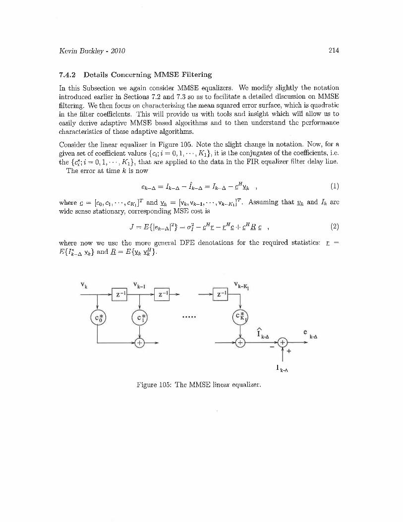


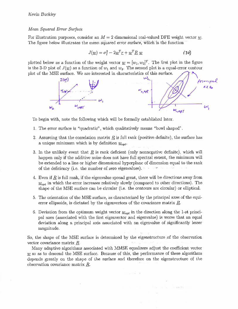
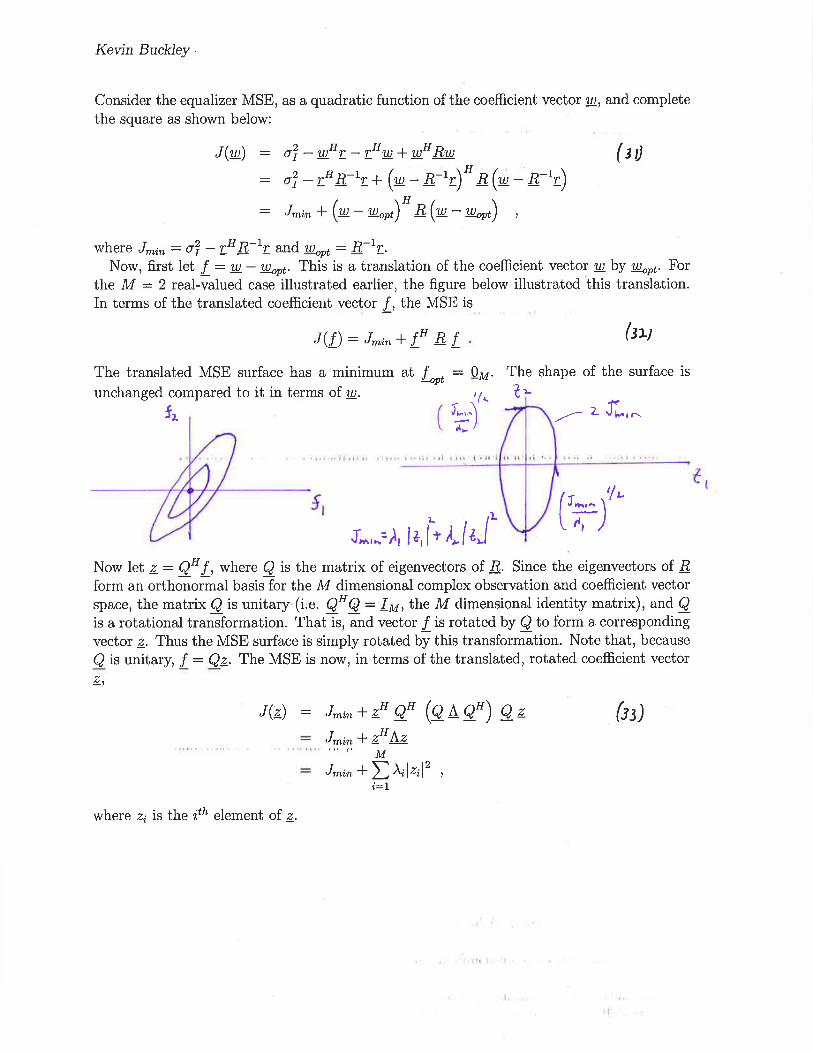


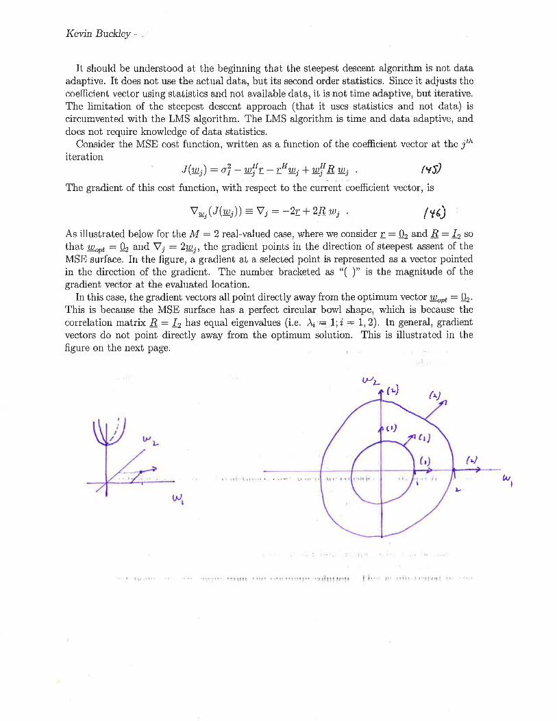
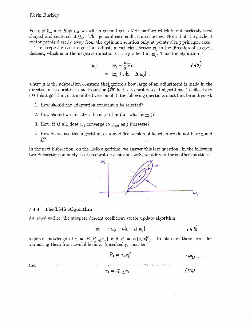
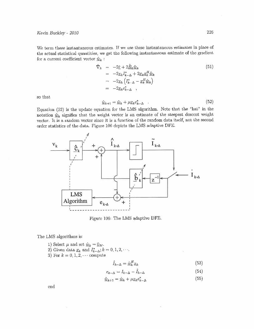


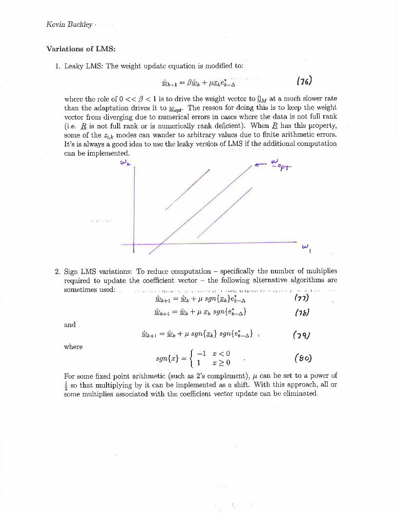


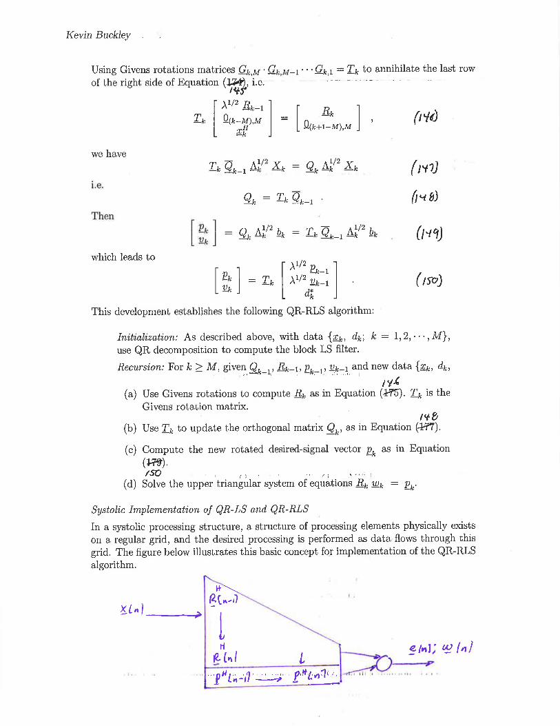


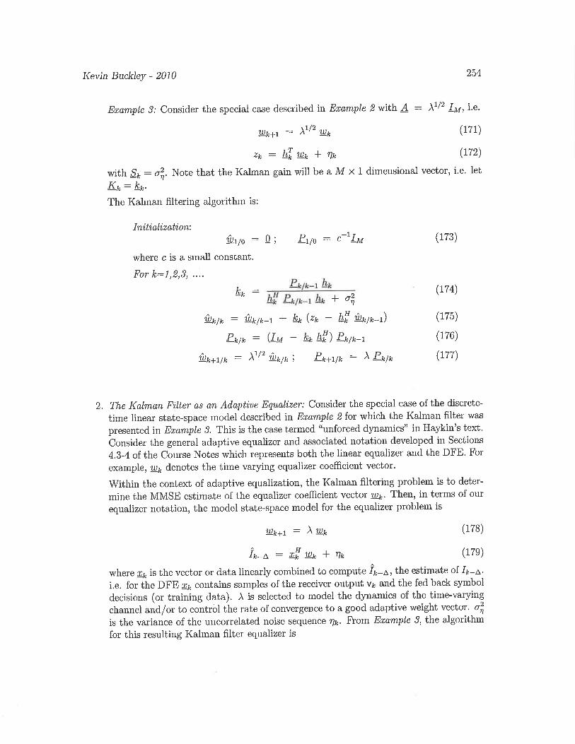
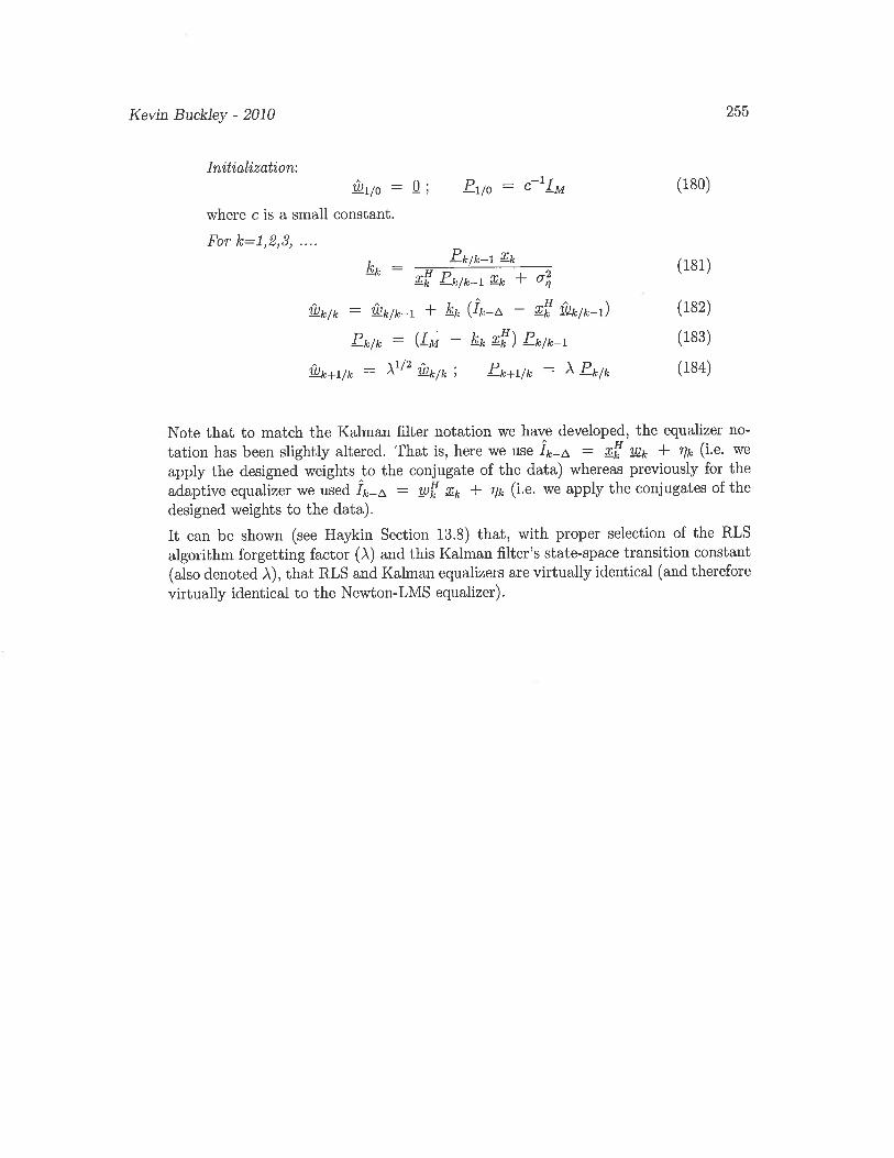

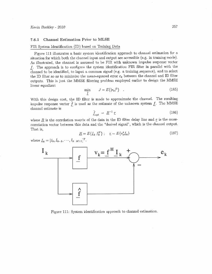

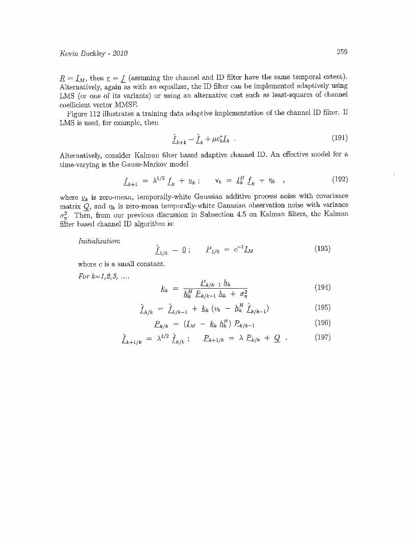
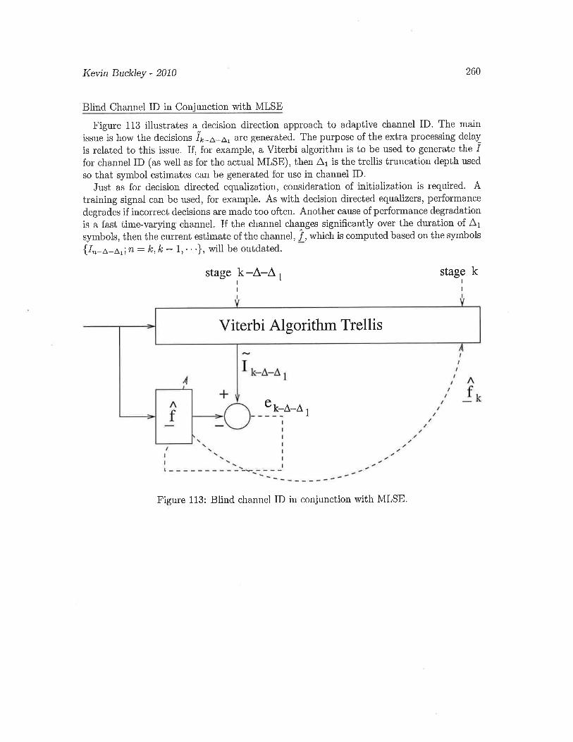


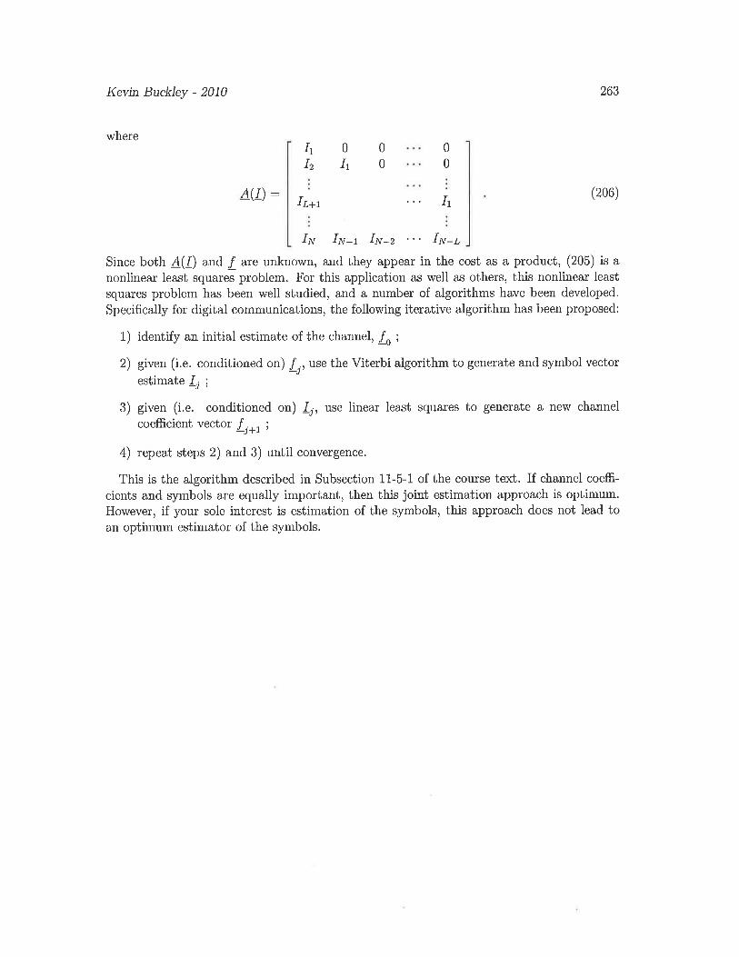

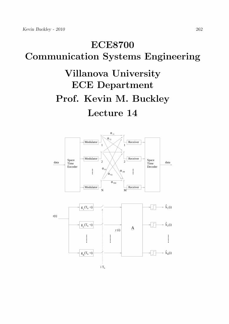
Kevin Buckley - 2010 262
ECE8700Communication Systems Engineering
Villanova UniversityECE Department
Prof. Kevin M. Buckley
Lecture 14
Modulator
Modulator
Modulator
SpaceTimeEncoder ....
1
2
N
dataSpaceTimeDecoder....
1
2 dataReceiver
Receiver
Receiver
M
α 11
α
αα
α
α
NM
1M
N2
N1
12
i Tb
g (T −t)b1
g (T −t)b2
g (T −t)bK
r (i) A
b (i)^1
b (i)2
b (i)K
r(t)
......
......
......

Kevin Buckley - 2010 263
Contents
8 Overview of Information Theory & Channel Coding 2658.1 Information Theory . . . . . . . . . . . . . . . . . . . . . . . . . . . . . . . . 2668.2 Block Codes . . . . . . . . . . . . . . . . . . . . . . . . . . . . . . . . . . . . 2678.3 Convolutional Codes . . . . . . . . . . . . . . . . . . . . . . . . . . . . . . . 2688.4 Turbo Codes . . . . . . . . . . . . . . . . . . . . . . . . . . . . . . . . . . . . 2698.5 Low Density Parity Check (LDPC) Block Codes . . . . . . . . . . . . . . . . 270
9 Space-Time Coding and MIMO Systems 2719.1 Multipath Fading Channels and Diversity Techniques . . . . . . . . . . . . . 271
9.1.1 Multipath Fading Channels . . . . . . . . . . . . . . . . . . . . . . . 2719.1.2 Diversity Techniques . . . . . . . . . . . . . . . . . . . . . . . . . . . 272
9.2 A Spatial Diversity Technique . . . . . . . . . . . . . . . . . . . . . . . . . . 2739.3 Space-Time Block Codes . . . . . . . . . . . . . . . . . . . . . . . . . . . . . 2759.4 Space Time Trellis Codes . . . . . . . . . . . . . . . . . . . . . . . . . . . . . 280
10 Spread Spectrum & Multiuser Communications 28110.1 Overview of Spread Spectrum Methods . . . . . . . . . . . . . . . . . . . . . 28210.2 Direct Sequence Code Division Multiple Access (DS-CDMA) . . . . . . . . . 28310.3 Multiuser CDMA . . . . . . . . . . . . . . . . . . . . . . . . . . . . . . . . . 288
10.3.1 Optimum Synchronous Receiver . . . . . . . . . . . . . . . . . . . . . 28910.3.2 Optimum Asynchronous Receiver . . . . . . . . . . . . . . . . . . . . 29210.3.3 Conventional “Single User” Matched Filter Detector . . . . . . . . . . 29410.3.4 Linear Estimators . . . . . . . . . . . . . . . . . . . . . . . . . . . . . 296

Kevin Buckley - 2010 264
List of Figures
114 Digital Communciation system block diagram. . . . . . . . . . . . . . . . . . 265115 Block code encoding. . . . . . . . . . . . . . . . . . . . . . . . . . . . . . . . 267116 A decoder block diagram for a RS code. . . . . . . . . . . . . . . . . . . . . 267117 Equivalent encoders in (a) controller canonical nonrecursive form; and (b)
systematic recursive form. . . . . . . . . . . . . . . . . . . . . . . . . . . . . 268118 The turbo encoder proposed by Berrou, Glavieux and Thitimajshima. . . . . 269119 Turbo code iterative decoder. . . . . . . . . . . . . . . . . . . . . . . . . . . 269120 A multipath channel. . . . . . . . . . . . . . . . . . . . . . . . . . . . . . . . 271121 A MIMO flat-fading communications channel. . . . . . . . . . . . . . . . . . 274122 The STBC transmitter. . . . . . . . . . . . . . . . . . . . . . . . . . . . . . . 275123 The Alamouti STBC transmitter and ML receiver for M = 1 receiving antenna.277124 Trellis diagram representation of symbol sequences for a flat-fading, Ms = 2
symbol modulation scheme. . . . . . . . . . . . . . . . . . . . . . . . . . . . 279125 Direct Sequence transmitter (shown for PSK) without CDMA. . . . . . . . . 283126 DS-CDMA modulation with a signature code. . . . . . . . . . . . . . . . . . 284127 DS-CDMA viewed as QPSK with a PN generated pulse shape g(t). . . . . . 285128 CDMA symbol detector - lowpass equivalent. . . . . . . . . . . . . . . . . . . 285129 Conditional pdf’s for CDMA detection. . . . . . . . . . . . . . . . . . . . . . 286130 Equivalent discrete-time ISI channel model for DS-CDMA. . . . . . . . . . . 287131 Typical CDMA user’s signature signal correlation function. . . . . . . . . . . 288132 Synchronous multiuser CDMA receiver front end. . . . . . . . . . . . . . . . 291133 Asynchronous multiuser CDMA receiver front end. . . . . . . . . . . . . . . 293134 Two CDMA users’ asynchronous pulse overlap. . . . . . . . . . . . . . . . . 293135 Suboptimum decoupled matched filter detector for asynchronous multiuser
CDMA. . . . . . . . . . . . . . . . . . . . . . . . . . . . . . . . . . . . . . . 294136 The linear receiver for asynchronous multiuser CDMA. . . . . . . . . . . . . 297137 The linear MMSE detector for synchronous multiuser CDMA. . . . . . . . . 298

Kevin Buckley - 2010 265
8 Overview of Information Theory & Channel Coding
This is a very brief overview of Information Theory and Coding for Digital Communications,the topic of ece8771.
Information theory is the principal foundation of modern digital communication, providinga theoretical basis for lossless source coding, lossly source coding and channel coding
Specifically, it provides theoretical performance limitations and, conversely, achievable per-formance capabilities
For channel coding, given a specific channel, information theory tells us what the maximumchannel capacity is for transmission of information without error
A very important aspect of this channel capacity bound is that the various forms of its proofare typically not constructive
Shannon’s Contributions: The sequence of two papers:
• C. Shannon, “A mathematical theory of communications”, Bell Systems Tech. Jour.,Vol. 27, pp. 379-423, 623-656, July-Oct., 1948.
built the foundation for information theory. It established nonconstructive proofs of Theo-rems on:
• Source information and lossless coding
• Lossly coding and rate distortion
• Channel capacity
sourceinformation
encodersource channel
encodercommunication
channel
compressedinformation bits
transmittedsignal
receivedsignal
ai
informationoutputdecoder
sourcechanneldecoder
receivedsignal
ai^
compressedinformation bits
estimated estimatedinformation
modulator
s (t) r (t)
information
demodulator
r (t)^ ^
j
j
x
x C
C k
k
estimated
codeword.bits
codewordbits
Figure 114: Digital Communciation system block diagram.

Kevin Buckley - 2010 266
8.1 Information Theory
We desire measures of information:
• Information replaces uncertainty with certainty
• Measures should quantify randomness of a random variable, between random variables,or of a random process
Entropy is the measure of average uncertainty. As applied to a communications channel, itprovides a lower bound on the rate of reliable communications (as measured in bits/channel-use or bits/second/Hertz).
Capacity of a Band-Limited Waveform Channel
Consider a channel of bandwidth 2W used over duration τs with AWGN. Say that the noisespectral level is N0, power per basis dimension is σ2
n. Let the total input power be P , sothat the power per bandwidth is P
2W. The channel capacity is:
C = W τs log2(1 +P
2Wσ2n
) (bits per channels use)
or
C = W log2(1 +P
2Wσ2n
) (bits/second)
= W log2(1 +P
N0 W) (bits/second)
The capacity is a ”simple” function of bandwidth W and SNR Pav
N0W. Capacity increases with
both bandwidth and SNR. As W → ∞, C approaches the asymptotic value:
C∞ = limW→∞
W log(
1 +P
N0W
)
= limW→∞
W log(e) ln(
1 +P
N0W
)
= limW→∞
W log(e)
(
P
N0Q+ · · ·
)
= W log(e)P
N0W= log(e)
P
N0.
So, increasing W has diminishing returns.
The Noisy Channel Coding TheoremThe issue is the relationship between capacity C, the bit rate R and symbol error proba-
bility Pe.
There exists codes and decoders that achieve reliable digital communication ifC > R. If R > C, reliable digital communication is not possible.
No assumption is made on the channel type. The proof of this theorem (i.e. the derivationof the results). makes use of very long random code words. The proof is effectively noncon-structive. A lot of research has been devoted to developing very long code word codes whichcan be generated and decoded in a computationally efficient manner. The state-of-the-artlong codes are turbo codes and Low Density Parity Check (LDPC) codes.

Kevin Buckley - 2010 267
8.2 Block Codes
information bits Channel
Encoder Channel ChannelDecoder Detection/Correction
Error CC
Automatic Repeat Request (ARQ)
Forward Error Correction (FEC)
Considering k information bits, we need M = 2k codewords. For (k, N) codes, there areN symbols/codeword, and the symbol alphabet size is q. No for binary (n, k) block codes,q = 2, n bits/codeword, and we require n > k.
Encoder Block
1 2 k3 .......
k information bits
1 ........2 3 N
N codeword symbols
Figure 115: Block code encoding.
For a (n, k) binary block code, with k length binary input vectors and n length binarycodewords, the code rate is: Rc = k
n(Rc < 1).
• The greater Rc is, the more efficient the code.
• The purpose of channel coding is to provide protection against transmission errors.Protection can improve in some sense as Rc decreases.
Common block codes:
• Hamming, Golay, Cyclic, BCH
• Reed-Soloman - nonbinary, described using Galois Fields
Soft and hard decision decoding; syndrome decoding.
e
correctionerror
Cmsyndrome
calculationerror patternY S
−+
identification enumerationerror pattern
Figure 116: A decoder block diagram for a RS code.
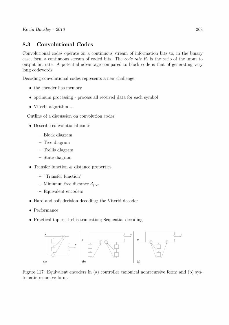
Kevin Buckley - 2010 268
8.3 Convolutional Codes
Convolutional codes operate on a continuous stream of information bits to, in the binarycase, form a continuous stream of coded bits. The code rate Rc is the ratio of the input tooutput bit rate. A potential advantage compared to block code is that of generating verylong codewords.
Decoding convolutional codes represents a new challenge:
• the encoder has memory
• optimum processing - process all received data for each symbol
• Viterbi algorithm ...
Outline of a discussion on convolution codes:
• Describe convolutional codes
– Block diagram
– Tree diagram
– Trellis diagram
– State diagram
• Transfer function & distance properties
– ”Transfer function”
– Minimum free distance dfree
– Equivalent encoders
• Hard and soft decision decoding; the Viterbi decoder
• Performance
• Practical topics: trellis truncation; Sequential decoding
x
c
x
c c
x
(b)(a) (c)
Figure 117: Equivalent encoders in (a) controller canonical nonrecursive form; and (b) sys-tematic recursive form.

Kevin Buckley - 2010 269
8.4 Turbo Codes
Concepts required to introduce Turbo block codes:
• Constituent codes (convolutional & block)
• Concatenated codes (specifically PCCC)
• Interleaving
C
C
π
j
y’ ; i=1,2, ...
j,1
j,2
jx’ ; j=1,2, ... , N
y’ ; j=1,2, ... , N
y’ ; j=1,2, ... , N
x’ ; j=1,2, ... , N
i
Convolutional
ConvolutionalEncoder
2
Encoder 1
Figure 118: The turbo encoder proposed by Berrou, Glavieux and Thitimajshima.
Key development: Decoding Algorithms Which Generate Extrinsic Information
• Symbol-by-symbol MAP and the BCJR algorithm:
L.R. Bahl, J. Cocke, F. Jelinek and J. Raviv, ”Optimal decoding of linearcodes for minimizing symbol error rate”, IEEE Trans. on Info. Theory, pp.284-287, Mar. 1974.
• Soft Output Viterbi Algorithm (SOVA):
J. Hagenauer and P. Hoeher, ”A Viterbi algorithm with soft-decision outputsand its applications”, Proc. of Globecom, pp. 1680-1686, 1989.
Decoder 2 π−1jx’
Decoder 1 π
π−1
jx’ L ( )(2)
e jx’ L ( )(2)
e
jx’ L ( )e
(1)jx’ L ( )e
(1)
j,1y
jx’ jx (2)
L ( ) − Lc
j,2y
jx π
jx’ jx L ( ) − Lc
(1)
Figure 119: Turbo code iterative decoder.

Kevin Buckley - 2010 270
8.5 Low Density Parity Check (LDPC) Block Codes
1962: Gallagher introduced LDPC block codes
He described these in terms of the parity check matrix H
Principal LDPC code characteristics: large size and sparseness of H
Large block codes, so potentially good performance
Example: a 9 × 12-dimensional parity check matrix
H =
1 1 1 1 0 0 0 0 0 0 0 00 1 1 0 1 0 0 1 0 0 0 01 0 1 1 0 0 0 0 1 0 0 01 0 0 0 0 0 1 0 1 1 0 00 1 0 0 1 0 1 0 0 0 1 00 0 0 1 0 1 0 0 0 0 1 10 0 0 0 1 0 0 1 1 0 1 00 0 0 0 0 1 0 1 0 1 0 10 0 0 0 0 1 1 0 0 1 0 1
In the 1960’s and 1970’s LDPC codes were largely ignored – impractical
1981: Tanner - LDPC codes + graph theory = iterative decoding algorithms
LDPC codes still virtually unnoticed until the mid 1990’s
1994: turbo codes shed light on LDPC codes
Advantages over turbo codes (no long interleaver, nearer to capacity performance, bettererror floor)
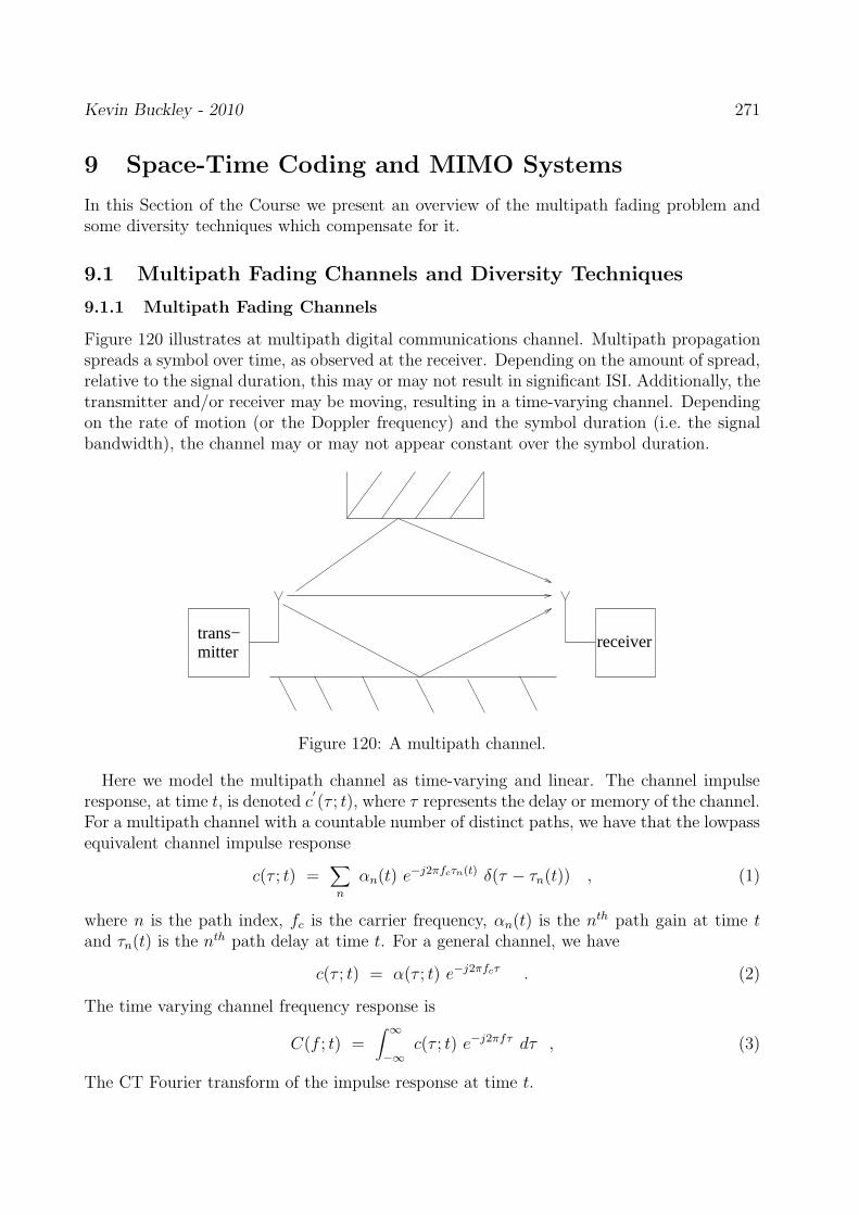
Kevin Buckley - 2010 271
9 Space-Time Coding and MIMO Systems
In this Section of the Course we present an overview of the multipath fading problem andsome diversity techniques which compensate for it.
9.1 Multipath Fading Channels and Diversity Techniques
9.1.1 Multipath Fading Channels
Figure 120 illustrates at multipath digital communications channel. Multipath propagationspreads a symbol over time, as observed at the receiver. Depending on the amount of spread,relative to the signal duration, this may or may not result in significant ISI. Additionally, thetransmitter and/or receiver may be moving, resulting in a time-varying channel. Dependingon the rate of motion (or the Doppler frequency) and the symbol duration (i.e. the signalbandwidth), the channel may or may not appear constant over the symbol duration.
trans−mitter
receiver
Figure 120: A multipath channel.
Here we model the multipath channel as time-varying and linear. The channel impulseresponse, at time t, is denoted c
′
(τ ; t), where τ represents the delay or memory of the channel.For a multipath channel with a countable number of distinct paths, we have that the lowpassequivalent channel impulse response
c(τ ; t) =∑
n
αn(t) e−j2πfcτn(t) δ(τ − τn(t)) , (1)
where n is the path index, fc is the carrier frequency, αn(t) is the nth path gain at time tand τn(t) is the nth path delay at time t. For a general channel, we have
c(τ ; t) = α(τ ; t) e−j2πfcτ . (2)
The time varying channel frequency response is
C(f ; t) =∫ ∞
−∞c(τ ; t) e−j2πfτ dτ , (3)
The CT Fourier transform of the impulse response at time t.

Kevin Buckley - 2010 272
Since the channel characteristics depend on the transmission environment, it is modeledas random. That is, the impulse response c(τ ; t) or equivalently the path gains and delayare considered random. If there are a large number of random paths, the impulse responsec(τ ; t) is often modeled as a complex-valued Gaussian process, in which case the envelope of
c(τ ; t), |c(τ ; t)| =√
Rec(τ ; t)2 + Imc(τ ; t)2, is Rayleigh distributed. If there are severalstrong, fixed paths, then the envelope is often modeled as Ricean.
For design purposes, multichannel fading channels are characterized in terms of severalparameters associated with the channel. For example:
1. Tm is the multipath temporal spread of the channel. It is the memory depth of thechannel impulse response.
2. (∆f)c ≈1
Tmis the coherence bandwidth of the channel. For frequencies separated by
∆f > (∆f)c, the channel frequency response C(f ; t) is effectively uncorrelated at anytime t.
3. Bd is the Doppler spread of the channel. It is the magnitude of the maximum variationof the carrier frequency due to transmitter/receiver motion.
4. (∆t)c ≈1
Bd
is the coherence time of the channel. For times separated by ∆t > (∆t)c,
the channel impulse response c(τ ; t) is effectively uncorrelated for any memory time τ .
Consider a digital communication modulation scheme that has symbol duration T andbandwidth W (in Hz.) Flat fading, or frequency nonselective fading, occurs when the impulseresponse is modeled as c(τ ; t) = c(t). It refers to the situation where T >> Tm (i.e. thesymbol duration is much greater than the channel spread). For modulations schemes whereW ≈ 1
T, the flat fading condition is equivalent to W << (∆f)c (i.e. the signal bandwidth is
much less than the coherence bandwidth of channel).A slowly fading or quasi-static channel refers to a channel that is effectively time invariant
over the symbol or processing interval. That is, when effectively c(τ ; t) = c(τ) which impliesthat T >> ∆tc.
For a flat fading, slowly fading channel, c(τ ; t) = c = α e−jφ. This implies thatTm Bd << 1. In this case, a for a Rayleigh fading channel, α is Rayleigh distributed andα2 (the symbol energy gain or loss) is chi-squared distributed.
9.1.2 Diversity Techniques
Channel fading can result in severe degradation in the performance of a digital communi-cation system. This is due to the fact the channel may be in a deep fade (i.e. the channelattenuation may be large) when some bits are transmitted. These bits will not be reli-ably received. Diversity is used to mitigate channel fading. Generally, diversity refers totransmitting information over different channel conditions. If diversity is designed properly,then these different channel conditions are uncorrelated, and the diversity is referred to amaximum diversity. There are various approaches to diversity. Three common approachesare:

Kevin Buckley - 2010 273
1. Temporal diversity, for which the information is sent through a channel spread outover time. Than is, it is sent over the same channel at different times. If the channel ittime varying, and it the different times are spread further than the channel coherencetime, we can think of the channel at different times as different channels or as havingdifferent channel conditions. Temporal diversity typically involves channel coding andinterleaving.
2. Frequency diversity, for which the information is sent through a channel, spread overfrequency. For example, Frequency Division Multiplexing (FDM) is used for this pur-pose, where take full advantage of frequency diversity the different frequency binsshould be separated by at least the channel coherence bandwidth. Channel codingtechniques have been adapted for this application.
Broadband modulation schemes, where W >> (∆f)c so that Tm << T , are alsoused to provide frequency diversity. If in addition to using broadband symbols, ifTm << T << (∆t)c so that the channel is quasi-static and there is no appreciable ISI,a RAKE receiver can be used. The RAKE receiver is essentially a discrete-time filtermatched to the symbol shape.
3. Spatial diversity, where multiple transmit and/or receiver antennae are used to transmitinformation over different physical channels. We discuss this diversity approach in moredetail in the next section.
In the following subsections we first discuss an approach which is applicable for known,flat-fading channels. This is referred to as spatial coding. Subsequently we consider space-time coding, for:
1. known, time-invariant, flat-fading channels;
2. unknown, time-varying, flat-fading channels; and
3. frequency-selective fading channels (unknown/unknown, time-invariant/time-varying).
9.2 A Spatial Diversity Technique
As a prelude to our study of space-time coding, we consider a spatial processing technique forknown, flat-fading channels. The parallels between this and temporal coding will be clear,suggesting that coding methods we have already covered might be considered for space-timecoding.
Assume that there are N transmitting antennae, and M receiver antennae. There areN × M channels, one from each transmitter antenna to each receiver antenna. We assumeeach channel is flat-fading and constant over a symbol duration, so that the channel from thenth transmitter to the mth receiver is a complex constant αmn. We assume that the M × Nmatrix
A =
α11 α12 · · · α1N
α21 α22 · · · α2N...
.... . .
...αM1 αM2 · · · α1MN
(4)

Kevin Buckley - 2010 274
of channel response constants is known. This Multiple Input Multiple Output (MIMO)channel is illustrated in Figure 121.
Modulator
Modulator
Modulator
SpaceTimeEncoder ....
1
2
N
dataSpaceTimeDecoder....
1
2 dataReceiver
Receiver
Receiver
M
α 11
α
αα
α
α
NM
1M
N2
N1
12
Figure 121: A MIMO flat-fading communications channel.
The input to the transmitter antenna array at time k is the set of N symbols in the vectord. At the receiver, at time k, our observation across the receiver antenna array after matchedfiltering and sampling is the M dimensional observation vector
y = A d + n (5)
where the additive noise vector n is assumed to be uncorrelated, zero-mean complex Gaussianwith correlation matrix σ2
nIM . The noise n and symbols d are assumed to be mutuallyuncorrelated. For now we assume that the sequence of d ′s is statistically independent overtime, and since the channels have no memory and the noise is temporally uncorrelated, atthe receiver we process our observations one symbol duration at a time.
Figure 121 illustrates how the transmitter generates a symbol vector from input infor-mation bits. Let Ms be the number of symbols of the modulation scheme, common to alltransmitters. There are MN
s possible symbol vectors d. Let K be the number of bits to betransmitted at a given symbol time, and let bi; i = 1, 2, · · · , Mv represent the possible vectorsof K bits to be transmitted over a symbol time (Mv = 2K). The ”serial to parallel” convertertakes each bi and maps it to a unique di symbol vector for transmission. (It is assumed thatMv ≤ MN
s .) The form of this mapping, called the spatial code, is not within the scope ofthis Course.
At the receiver, the objective is to decide, from the observation y, which symbol vectorfrom di; i = 1, 2, · · · , Mv and corresponding information bit vector bi was sent. This is thereceiver detection problem.
Several receiver detection approaches have been suggested. Here we consider the MaximumLikelihood (ML) detector. Under the Gaussian receiver noise assumption stated above, thejoint pdf of the received data, y, conditioned on a transmitted symbol vector di, is
p(y/di) =1
(πσn)2Ne−||y−A d
i||2/σ2
n . (6)

Kevin Buckley - 2010 275
The ML detection problem ismax
di
p(y/di) (7)
ormin
di
||y − A di||2 . (8)
9.3 Space-Time Block Codes
Space-Time Processing for Known, Time-Invariant, Flat-Fading Channels
Though there had been some isolated developments in joint spatial and temporal diversityearlier in the 1990’s (e.g. the delay diversity transmitter), the origin of the general space-timecoding approach in the open literature dates back only to 1998 with the publication of V.Tarokh, N. Seshadri and A. R. Calderbank [1]. In this paper, space-time coding criteria weredeveloped, and trellis space-time codes for flat-fading (no ISI), time-invariant (quasi-static)channels were considered in detail. Two space-time code design/performance criteria wereestablished, which deal with the differences between pairs of space-time code matrices. Thesecriteria, a rank criterion and a determinant criterion, will be presented below. They can bethought of as generalizations of the distance criterion for block channel codes.
Below, we will focus on space-time block codes (STBC’s), which compared to trellis space-time codes are conceptually simpler and have reduced receiver complexity. STBC’s anddecoding can be thought of as a generalization of the spatial diversity approach describedabove.
Consider transmitting a block of T symbols (time slots) over each of N transmit antennaeusing a Ms symbol modulation scheme. Let cn,t be the symbol transmitted from the nth
antenna at symbol time t. The matrix
C =
c1,1 c1,2 · · · c1,T
c2,1 c2,2 · · · α2,T...
.... . .
...CN,1 αN,2 · · · αN,T
(9)
is a code matrix. There are MNTs possible code matrices. Let K be the number of bits to
be represented by a code matrix C. Figure 122 depicts the STBC transmitter.
Space Time
Block Coder
(STBC)
Modulator
Modulator
Modulator
c ......... c2,1 2,T
c ......... cN,1 N,T
b = [ b , b , .... , b ]K21
1
2
N
....
c ......... c1,T1,1
Figure 122: The STBC transmitter.

Kevin Buckley - 2010 276
With Mb = 2K , let bm; m = 1, 2, · · · , Mb represent all possible K-bit vectors. A STBCis a mapping for each bm to a unique Cm code matrix. Let Cm; m = 1, 2, · · · , Mb bethe set code matrices for a STBC. From the MNT
s possible code matrices, we should choosethe Cm; m = 1, 2, · · · , Mb to be in some meaningful sense as different from one another aspossible.
Recall that for block codes, the principal measure dictating performance is dmin, theminimum Hamming distance between codewords. We now describe analogous measuresfor STBC’s. Assume the channels are memoryless and time-invariant. Let the αij be thecomplex, Gaussian channel gain from transmitter i to receiver j. For zero mean αij , thechannel is Rayleigh fading. Let Bmk = Cm − Ck, and let Amk = BmkB
Hmk. Denote as
λi; i = 1, 2, · · · , R the nonzero eigenvalues of Amk. For Rayleigh fading channels, using anML receiver, the probability of detecting Ck given that Cm was transmitted, is bounded as
P (Ck/Cm) ≤
(
R∏
i=1
λi
)−N(
Es
4N0
)−RM
(10)
where, as before, M is the number of receiver antennae.
• The diversity advantage, (RM), is the power on the inverse SNR(
Es
4N0
)−1. The bigger,
the better.
• The rank criterion states that the difference matrix Bmk should be full rank for allm 6= k; m, k = 1, 2, · · · , Mb. Then R = N is maximum.
• The coding advantage,(
∏Ri=1 λi
)−M, is the gain over an uncoded system with same
diversity.
• The determinant criterion states that if R = N , the minimum determinant |Amk|, overallm 6= k; m, k = 1, 2, · · · , Mb, should be maximized.
Let rj(t); j = 1, 2, · · · , M ; t = 1, 2, · · · , T be the data received by the jth receiver atsymbol time t during over the duration of a code matrix transmission. Let r be the NT -dimensional received data vector for a transmitted code matrix. The ML estimator is thesolution to:
Cm = arg maxC
i
p(r/Ci) (11)
A popular STBC for N = 2 transmitting antennae and T = 2 time slots was proposed inAlamouti [2]. Assuming an Ms symbol modulation scheme, let ci; i = 1, 2 be two symbolsthat represent K = 2 · log2(Ms) bits. The Mv code matrices representing the K bits are ofthe form
C =
[
c1 −c∗2c2 c∗1
]
. (12)
This STBC has a code rate equal to 1 (i.e. on the average, one symbol per symbol-time istransmitted). Besides having good diversity characteristics (i.e. it satisfies the rank criterion),this STBC, called the Alamouti code, results is a particularly simple ML decoding structure.

Kevin Buckley - 2010 277
At the receiver, a simple preprocessor, termed as space-time matched filter, can be usedto decouple the ML estimation of c1 and c2. Figure 123 illustrates the decoder for the M = 1receiver antenna case. (We now use h to represent channel response.)
Modulator
1 c , − c2**
2 c , c1*
receiver,ser.−to−par. HH
r
c 2^
c1 1
2
Modulator
h
h
1
2
Figure 123: The Alamouti STBC transmitter and ML receiver for M = 1 receiving antenna.
The received data vector is
r =
[
r1
r∗2
]
=
[
h1 h2
−h∗1 h∗
2
] [
c1
c2
]
+
[
n1
n∗2
]
= H c + n . (13)
Since the columns of H are orthogonal, H−1 ∝ HH , and
y =
[
y1
y2
]
= HH r = (|h1|2 + |h2|
2)
[
c1
c2
]
+
[
n′
1
n′
2
]
, (14)
where n′
1 and n′
2 are uncorrelated because n1 and n∗2 are uncorrelated and equal-variance, and
HH is unitary to within a scalar. Thus, y1 and y2 can be processed separately to optimallyestimate c1 and c2, respectively. HH is the space-time matched filter.
The Alamouti STBC was extended to N = 4 and N = 8 transmit antennae in a paperby V. Tarokh, H. Jsfsrkhsni and A. R. Calderbank [3], 1999, on orthogonal STBC’s. Goodnonorthogonal codes for N = 3, 5, 6and7 codes are also described.
Space-Time Processing for Unknown, Time-Varying, Flat-Fading Channels
We just discussed STBC’s for flat-fading, quasi-static channels. Quasi-static means thatthe channel responses did not change over the temporal length of a STBC matrix. Forexample, the STBC proposed by Alamouti was designed for channels that can be assumedto be constant over two successive symbol time slots, and for decoupled optimum decodingthe channel responses were assumed constant over the block, and known at the receiver.Even though in the design of these STBC’s, quasi-static channels are assumed, these codescan be used for channels which are varying over a code block duration. However, the decoderstructures designed under the quasi-static assumption will likely not be optimum. We nowconsider STBC decoding for unknown, time-varying, flat-fading channels. Specifically, as anexample, we consider decoding of the Alamouti STBC. We will consider both the exact MLdecoder and a computationally efficient suboptimum decoder.
First we need a little background on MLSE for unknown, time-varying channels. Considerthe single transmitter antenna, single receiver antenna case. Let h[n] be the unknown, time-varying, flat-fading channel response, that is modeled as
h[n + 1] = c · h[n] + w[n] , (15)

Kevin Buckley - 2010 278
where c is a known complex constant with |c| < 1, and w[n] is an uncorrelated Gaussianrandom process. This is a first order Gauss-Markov channel model. Consider transmissionof n symbols Ik; k = 1, 2, · · · , n, received in AWGN, as
rk = Ik + nk ; k = 1, 2, · · · , n . (16)
The joint pdf of the received data, conditioned on the channel coefficients and symbols, is
p(r/I, h) =1
(2πσ2)ne−
1
σ2
∑
n
k=1|rk−hk·Ik|2 (17)
where σ2 is the variance of the noise nk. Marginalizing over h, the joint pdf of r conditionedof I is
p(r/I) =∫
hp(r/I, h) p(h) dh . (18)
The MLSE problem ismax
Ip(r/I) (19)
where the data r has been plugged into p(r/I) (i.e. maximize the likelihood function).The key point here is that Eq (19) does not reduce to a decoupled symbol-by-symbol
detection receiver. This is because of the correlation over time of the unknown channelresponse. Because of this, data at all time can be effectively used to estimate the symbol atany time.
We know that for a Ms symbol modulation scheme, the number of possible I sequencesup to time n is Mn
s . Figure 124 shows the trellis representation of these possible sequencesfor Ms = 2. Each sequence is a path through the trellis. It has been shown, for exam-ple in Iltis [4] and Chen, Perry and Buckley [5], that for each possible sequence, the costp(r/I) =
∫
h p(r/I, h)p(h)dh is computed using a channel estimator which is conditioned onthat sequence. The Iltis paper shows that, for the Gauss-Markov channel model such asdescribed above, the conditional channel estimator can be implemented as a Kalman filter(see Iltis for details). The conditional channel estimate generated for each sequence will be afunction of the entire sequence and data history. So, in terms of the trellis representation, aKalman channel estimator must be run for each path through the trellis. Since this Kalmanestimator has memory back to time k = 0, each path through a branch will have its ownbranch cost, which means that any path into a state, regardless of its current cost relativeto other paths into that state, might turn out to be the best path sometime in the future.Thus, no optimum pruning of paths is possible. The Viterbi algorithm can not be optimallyapplied, and the MLSE solution requires computation of all Mn
s sequence costs. This, ofcourse, is not practical for large n.
In Chen, Perry and Buckley [5] a suboptimum but effective pruning algorithm, based onthe List Viterbi algorithm, is described. The algorithm is in the general sequence estimatorclass of Per-Survivor Processing (PSP) algorithms, because a conditional Kalman channelestimator is used for each survivor (unpruned) sequence.
Returning to decoding algorithms for the Alamouti STBC for unknown, time-varying, flat-fading channels, consider a sequence of transmitted STBC matrices, Ck; k = 1, 2, · · · , n, andreceived data rk; k = 1, 2, · · · , n, where rk is the received data for block k. For notational

Kevin Buckley - 2010 279
stages (k)
k=0 k=1 k=2 k=n−1 k=n+1k=n
(−1)
states ..... .....
(1)
Figure 124: Trellis diagram representation of symbol sequences for a flat-fading, Ms = 2symbol modulation scheme.
simplicity, assume M = 1 receiving antenna, so that rk = [r1,k, r∗2,k]
T , the two receiverantenna outputs for the two time slots corresponding to the reception of the Ck transmittedSTBC matrix. Let the two channels between the two transmitter antennae and the onereceiver antenna be modeled as
hi[l + 1] = ci · hi[l] + wi[l]; i = 1, 2 (20)
i.e. two Gauss-Markov channels with known c′is. Let
Hk =
[
h1[2k − 1] h2[2k − 1]−h∗
1[2k] h∗2[2k]
]
. (21)
Assume that the receiver noise is AWGN.
Let C = [C1, C2, · · · , Cn], R = [r1, r2, · · · , rn], and H = [H1, H2, · · · , Hn]. The MLSEproblem is:
maxC
p(R/C) (22)
p(R/C) =∫
Hp(R/C,H) p(H) dH (23)
and
p(R/C,H) =1
(2πσ2)2ne−
1
σ2
∑
n
k=1|r
k−H
k·c
k|2 (24)
Because of the correlation across time of the unknown, time-varying channel responses,solution of the MLSE problem, Eq (22), requires an exhaustive search of all STBC matrixsequences C. Since this is impractical, a PSP based algorithm similar to the one describedin the Chen paper can be employed.
Another suboptimum decoding algorithm for the Alamouti STBC for unknown, time-varying, flat-fading channels is described in Liu, Ma and Giannakis [6]. This algorithm,instead of using a conditional Kalman channel estimator for each sequence, runs a singleKalman filter channel estimator conditioned on a single estimated sequence.
Space-Time Processing for Unknown, Time-Varying, Frequency-Selective Fading Channels
For unknown, quasi-static, frequency selective (ISI) channels, a generalization of the Alam-outi STBC has recently been proposed in Lindskog and Paulraj [7]. The proposed code isreferred to as the Time-Reversed STBC (TR-STBC). Code matrices are 2×P dimensional,
Kevin Buckley - 2010 280
where P ≥ 2 (P = 2 for the Alamouti STBC). For P > 2, code matrices contain more thantwo information symbols, and pilot (known) symbols are inserted and used at the receiverto estimate the ISI channel, which is assumed constant over the P time slot transmissionduration of a code matrix. As with the Alamouti STBC, code matrices are constructed sothat a simple space-time matched filter can be used at the receiver to decouple the estimationof two sets of symbols.
For ISI channels that vary over a code matrix duration, a TR-STBC can still be used.However, the decoupling receiver can not be employed, and the pilot bit approach to chan-nel estimation can no longer be exploited. Alternatively, for any STBC, whether designedspecifically for ISI channels or not, a MLSE based PSP algorithm can be used. (See, forexample, Wang, Buckley and Perry [8].)
9.4 Space Time Trellis Codes
References
1. V. Tarokh, N. Seshadri and A. R. Calderbank, ”Space-time codes for high data ratewireless communications: Performance criterion and code construction”, IEEE Trans.Inform. Theory”, Vol 44, pp. 744-765, March 1998
2. S. M. Alamouti, ”A simple transmit diversity technique for wireless communications”,IEEE J. Select. Areas Commun., Vol 16, pp. 1451-1458, Oct. 1998.
3. ”V. Tarokh, H. Jafarkhani and A. R. Calderbank, ”Space-time block codes from or-thogonal designs”, IEEE Trans. Inform. Theory, Vol. 45, pp. 1456-1467, July 1999.
4. R. A. Iltis, ”A Bayesian maximum likelihood sequence estimation algorithm for a prioriunknown channels with symbol timing”, IEEE Jour. on Select. Areas in Comm., Vol.10, pp. 579-588, April 1992.
5. H. Chen, R. Perry and K. Buckley, ”Direct and EM based MAP sequence estimationwith unknown time-varying channels, ICASSP-2001, April, 2001.
6. Z. Liu, X. Ma and G.B.Giannakis, “Space-time coding and Kalman filtering for time-selective fading channels”, IEEE Trans. on Communications, Vol. 50, pp. 183-186,Feb. 2002.
7. E. Lindskog and A. Paulraj, ”A transmit diversity scheme for for channels with inter-symbol interference”, IEEE Intl Conf. on Commun., pp. 307-311, June, 2000.
8. C. Wang, K. Buckley and R. Perry, Space-time block coding over unknown frequencyand time selective channels”, CISS Conf., April 2003.

Kevin Buckley - 2010 281
10 Spread Spectrum & Multiuser Communications
There are several reasons for using a spread spectrum scheme for digital communications.Two historical reasons, motivated in large part by military applications, are: interferencemitigation – a narrow band interference signal will corrupt only a fraction of the communi-cations bandwidth; and security – signal transmission power spread over a large bandwidthwill be difficult to detect. A third reason, which has become particularly important with theadvent of mobile cellular systems, is added multiuser capacity.
Some of the more important communication theory and signal processing issues associatedwith spread spectrum systems are:
1. modulation (e.g. FSK, PSK, QPSK), and spectral spreading and multiuser multiplex-ing (e.g. TDMA, frequency hopping, direct sequence CDMA (DS-CDMA)) schemes;
2. spreading code;
3. capacity, efficiency and bandwidth;
4. synchronization (e.g. carrier and bit);
5. matched filtering and fractional sampling;
6. ISI, signal fading, interference and multiple users;
7. symbol error rate and mean squared error;
8. detection, sequence estimation, equalization and interference reduction;
9. training and decision directed modes;
10. power control, hand off, and antenna diversity; and
11. multichannel (i.e. multiple antenna) processing.
After a brief general introduction, our focus will be on DS-CDMA, consideration of basicmultiuser issues, and an overview of sequence estimation.

Kevin Buckley - 2010 282
10.1 Overview of Spread Spectrum Methods
Consider a bit rate of R bits/sec. (that is, R bps). More generally, R could be the symbolrate. The bit interval is
Tb =1
R. (25)
R, or Tb, dictate the transmission bandwidth if R bps are transmitted directly.Three methods which effectively increase the transmission bandwidth (spread the spec-
trum) are:
1. Frequency Hopping (FH): Over a bit interval Tb, the carrier frequency is switched anumber of times, according to some pseudo-random sequencing scheme dictated by aPN (pseudo noise) generated code.
2. TDMA (time-division multiple access): Strictly speaking, this is not a spread spectrummethod. However, if only a fraction of the time is allocated to a user to transmit, toachieve an average rate of R bps, shorter duration symbols must be crammed into asmaller allocated time slot, effectively increasing transmission bandwidth.
3. DS-CDMA: As described in detail below, instead of representing a bit as a single pulse,it is represented as a sequence (called a code signature) of short pulses (called chips).Compared to a single pulse, the chips of the code are much smaller in duration. Thusthe transmission spectrum is spread.
These issues are discussed in detail in Chapter 12 of the Course Text.
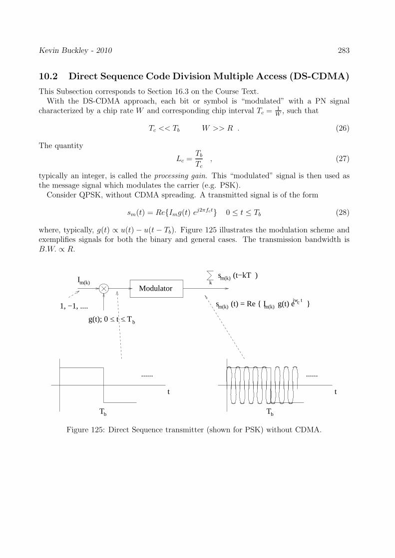
Kevin Buckley - 2010 283
10.2 Direct Sequence Code Division Multiple Access (DS-CDMA)
This Subsection corresponds to Section 16.3 on the Course Text.With the DS-CDMA approach, each bit or symbol is “modulated” with a PN signal
characterized by a chip rate W and corresponding chip interval Tc = 1W
, such that
Tc << Tb W >> R . (26)
The quantity
Lc =Tb
Tc
, (27)
typically an integer, is called the processing gain. This “modulated” signal is then used asthe message signal which modulates the carrier (e.g. PSK).
Consider QPSK, without CDMA spreading. A transmitted signal is of the form
sm(t) = ReImg(t) ej2πfct 0 ≤ t ≤ Tb (28)
where, typically, g(t) ∝ u(t) − u(t − Tb). Figure 125 illustrates the modulation scheme andexemplifies signals for both the binary and general cases. The transmission bandwidth isB.W. ∝ R.
Im(k)s (t−kT )m(k)
k
jw tcm(k) m(k)s (t) = Re I g(t) e
g(t); 0 < t < Tb
Tb
t
Tb
t
Modulator
1, −1, ....
............
Figure 125: Direct Sequence transmitter (shown for PSK) without CDMA.

Kevin Buckley - 2010 284
As stated above, with DS-CDMA the information sequence Ik is first modulated with asignature code. This is illustrated in the Figure 126 for a binary information sequence bi(k),which has rate is R. This sequence is mixed with a chip sequence cj (of rate 1
Tcwhere Tc is the
chip interval) to form a bipolar sequence aj = (bi⊕cj)·2−1. This sequence is modulated witha pulse shape g(t), which is typically rectangular. This signal then modulates the carrier.The resulting transmission bandwidth has B.W. ∝ W = LcR.
Modulatorbi(k)
jc (0,1)
ja = ( b c ) 2 − 1i j
ja (−1,1)
Tct
rate: 1/Tc
rate: 1/Tb
Tc Tb
....t
....
BW L Rc
p(t); 0 < t < T
1, 0, 0 ....
c
Figure 126: DS-CDMA modulation with a signature code.
The chip sequence cj is generated using a pseudo noise (PN) generator which generates theuser’s code sequence. The PN sequence is periodic, and although its period is not necessarilyLc, we will restrict our discussion to PN signature sequences with period Lc. Then, let
g(t) =Lc∑
j=1
cj p(t − jTc) 0 ≤ t ≤ Tb ; p(t) =
1 0 ≤ t ≤ Tc
0 otherwise(29)
where now ci = ±1 according to the PN sequence. Figure 127 illustrates the modulationscheme. Im(k) is the information sequence.
Note that this now looks like QPSK modulation as we have previously viewed it, exceptthat now we have a much more intricate pulse shape g(t). This viewpoint allows us to useresults from previous topics (e.g. detection, MLSE, equalization) directly! That is, we canstill identify an equivalent lowpass representation, and a discrete-time ISI channel model,that account for modulation/demodulation, matched filtering and perhaps whitening.
If the PN sequence is not periodic with period Lc, then demodulation and matched filter-ing/whitening is a little more complicated, but we can still develop an equivalent lowpassrepresentation, and discrete-time ISI channel model.
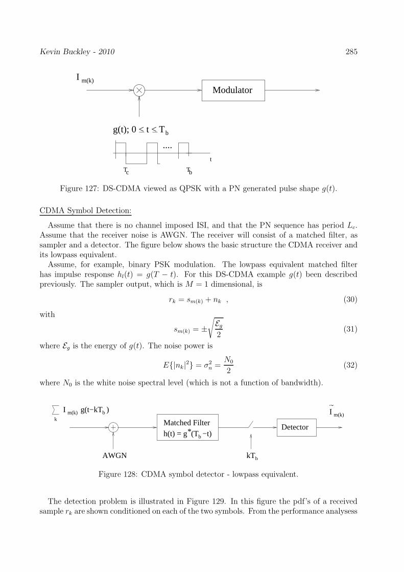
Kevin Buckley - 2010 285
ModulatorI m(k)
Tc Tb
....t
g(t); 0 < t < Tb
Figure 127: DS-CDMA viewed as QPSK with a PN generated pulse shape g(t).
CDMA Symbol Detection:
Assume that there is no channel imposed ISI, and that the PN sequence has period Lc.Assume that the receiver noise is AWGN. The receiver will consist of a matched filter, assampler and a detector. The figure below shows the basic structure the CDMA receiver andits lowpass equivalent.
Assume, for example, binary PSK modulation. The lowpass equivalent matched filterhas impulse response hl(t) = g(T − t). For this DS-CDMA example g(t) been describedpreviously. The sampler output, which is M = 1 dimensional, is
rk = sm(k) + nk , (30)
with
sm(k) = ±
√
Eg
2(31)
where Eg is the energy of g(t). The noise power is
E|nk|2 = σ2
n =N0
2(32)
where N0 is the white noise spectral level (which is not a function of bandwidth).
Matched Filter* h(t) = g (T −t)b
Detector
I m(k)I m(k) g(t−kT )
kb
bkT
~
AWGN
Figure 128: CDMA symbol detector - lowpass equivalent.
The detection problem is illustrated in Figure 129. In this figure the pdf’s of a receivedsample rk are shown conditioned on each of the two symbols. From the performance analysess
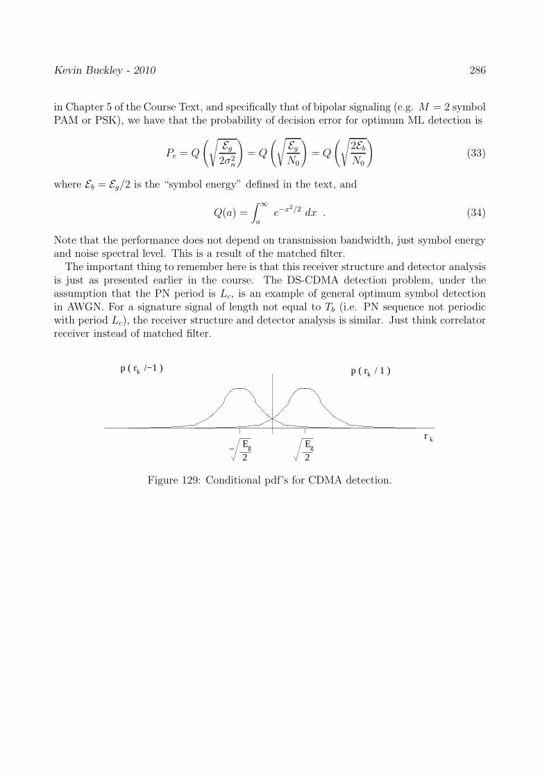
Kevin Buckley - 2010 286
in Chapter 5 of the Course Text, and specifically that of bipolar signaling (e.g. M = 2 symbolPAM or PSK), we have that the probability of decision error for optimum ML detection is
Pe = Q
(√
Eg
2σ2n
)
= Q
(
√
Eg
N0
)
= Q
(
√
2Eb
N0
)
(33)
where Eb = Eg/2 is the “symbol energy” defined in the text, and
Q(a) =∫ ∞
ae−x2/2 dx . (34)
Note that the performance does not depend on transmission bandwidth, just symbol energyand noise spectral level. This is a result of the matched filter.
The important thing to remember here is that this receiver structure and detector analysisis just as presented earlier in the course. The DS-CDMA detection problem, under theassumption that the PN period is Lc, is an example of general optimum symbol detectionin AWGN. For a signature signal of length not equal to Tb (i.e. PN sequence not periodicwith period Lc), the receiver structure and detector analysis is similar. Just think correlatorreceiver instead of matched filter.
Eg
2Eg
2
r
p ( r /−1 ) p ( r / 1 )
k
kk
−
Figure 129: Conditional pdf’s for CDMA detection.
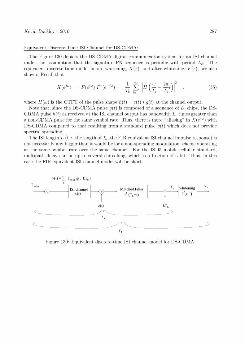
Kevin Buckley - 2010 287
Equivalent Discrete-Time ISI Channel for DS-CDMA:
The Figure 130 depicts the DS-CDMA digital communication system for an ISI channelunder the assumption that the signature PN sequence is periodic with period Lc. Theequivalent discrete-time model before whitening, X(z), and after whitening, F (z), are alsoshown. Recall that
X(ejω) = F (ejω) F ∗(e−jω) =1
Tb
∞∑
l=−
∣
∣
∣
∣
H(
ω
Tb
−2π
Tb
l)∣
∣
∣
∣
2
, (35)
where H(ω) is the CTFT of the pulse shape h(t) = c(t) ∗ g(t) at the channel output.Note that, since the DS-CDMA pulse g(t) is composed of a sequence of Lc chips, the DS-
CDMA pulse h(t) as received at the ISI channel output has bandwidth Lc times greater thana non-CDMA pulse for the same symbol rate. Thus, there is more “aliasing” in X(ejω) withDS-CDMA compared to that resulting from a standard pulse g(t) which does not providespectral spreading.
The ISI length L (i.e. the length of fk, the FIR equivalent ISI channel impulse response) isnot necessarily any bigger than it would be for a non-spreading modulation scheme operatingat the same symbol rate over the same channel. For the IS-95 mobile cellular standard,multipath delay can be up to several chips long, which is a fraction of a bit. Thus, in thiscase the FIR equivalent ISI channel model will be short.
ISI channelc(t)
bkT
Matched Filter
*h (T −t)bF (z )
* −1
whiteningyk
vkI m(k)
I m(k) v(t) = g(t−kT )k
b
xk
kf
z(t)
Figure 130: Equivalent discrete-time ISI channel model for DS-CDMA.
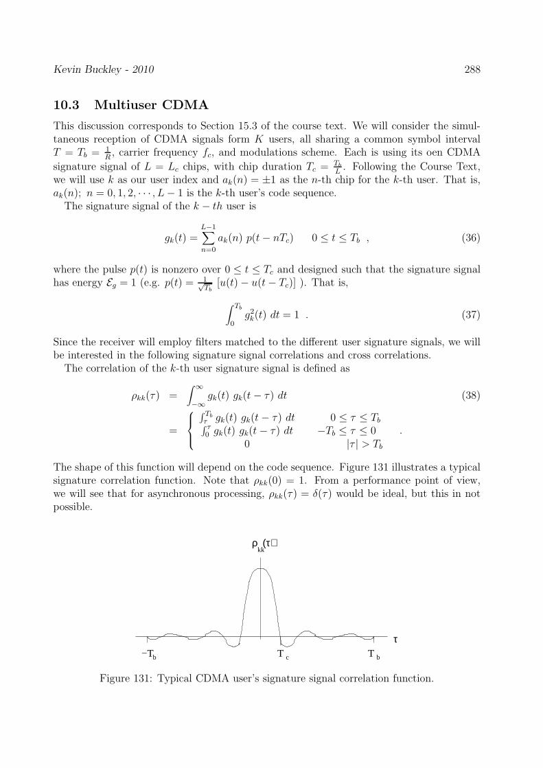
Kevin Buckley - 2010 288
10.3 Multiuser CDMA
This discussion corresponds to Section 15.3 of the course text. We will consider the simul-taneous reception of CDMA signals form K users, all sharing a common symbol intervalT = Tb = 1
R, carrier frequency fc, and modulations scheme. Each is using its oen CDMA
signature signal of L = Lc chips, with chip duration Tc = Tb
L. Following the Course Text,
we will use k as our user index and ak(n) = ±1 as the n-th chip for the k-th user. That is,ak(n); n = 0, 1, 2, · · · , L − 1 is the k-th user’s code sequence.
The signature signal of the k − th user is
gk(t) =L−1∑
n=0
ak(n) p(t − nTc) 0 ≤ t ≤ Tb , (36)
where the pulse p(t) is nonzero over 0 ≤ t ≤ Tc and designed such that the signature signalhas energy Eg = 1 (e.g. p(t) = 1√
Tb
[u(t) − u(t − Tc)] ). That is,
∫ Tb
0g2
k(t) dt = 1 . (37)
Since the receiver will employ filters matched to the different user signature signals, we willbe interested in the following signature signal correlations and cross correlations.
The correlation of the k-th user signature signal is defined as
ρkk(τ) =∫ ∞
−∞gk(t) gk(t − τ) dt (38)
=
∫ Tb
τ gk(t) gk(t − τ) dt 0 ≤ τ ≤ Tb∫ τ0 gk(t) gk(t − τ) dt −Tb ≤ τ ≤ 0
0 |τ | > Tb
.
The shape of this function will depend on the code sequence. Figure 131 illustrates a typicalsignature correlation function. Note that ρkk(0) = 1. From a performance point of view,we will see that for asynchronous processing, ρkk(τ) = δ(τ) would be ideal, but this in notpossible.
ρ (τ)kk
T b−Tb T c
τ
Figure 131: Typical CDMA user’s signature signal correlation function.

Kevin Buckley - 2010 289
The cross correlation between the signature signals of users j and k is defined as
ρjk(τ) =∫ ∞
−∞gk(t) gj(t − τ) dt (39)
=
∫ Tb
τ gk(t) gj(t − τ) dt 0 ≤ τ ≤ Tb∫ τ0 gk(t) gj(t − τ) dt −Tb ≤ τ ≤ 0
0 |τ | > Tb
.
Note that ρkj(τ) = ρjk(τ). Ideally, for multiuser reception, when k 6= j, ρkj(τ) = 0 for all τ .Again, the ideal is not possible.
Consider N symbols transmitted per user. Let the k-th user’s symbol vector be denotedas
bk = [ bk(1), bk(2), · · · , bk(N) ]T , (40)
where bk(i) is the k-th user’s i-th symbol. For the k-th user, the received signal (lowpassequivalent) is
sk(t − τk) =√
Ek
N∑
i=1
bk(i) gk(t − iTb) , (41)
τk is the propagation delay for the k − th user and Ek is the received energy per signaturesignal. Given all K users observed in noise, the corresponding received signal is
r(t) =K∑
k=1
sk(t − τk) + n(t) (42)
where n(t) is AWGN with spectral level N0
2. For (symbol) synchronous transmission, we
assume that τk = 0; k = 1, 2, · · · , K.The multiuser CDMA receiver problem is, basically, to detect or “estimate” the KN
symbols bk(i); 1 ≤ k ≤ K; 1 ≤ n ≤ N .
10.3.1 Optimum Synchronous Receiver
Here we assume that τk = 0; k = 1, 2, · · · , K. That is, some control of the transmitters hasbeen implemented to assure that the K user received signals are symbol synchronized. Alsowe assume here that there is no ISI. Then
r(t) =K∑
k=1
√
Ek bk(i) gk(t − iTb) + n(t) (i − 1)Tb ≤ t ≤ iTb , (43)
where n(t) is AWGN. We also assume that all KN symbols are mutually statistically in-dependent. Then, r(t) over (i − 1)Tb ≤ t ≤ iTb is statistically related to only the symbolsbk(i); k = 1, 2, · · · , K. Under these assumptions we have a generalization of the single

Kevin Buckley - 2010 290
user detection problem studied earlier in the course. That is, the optimum symbol detec-tor processes r(t) over only the interval (i − 1)Tb ≤ t ≤ iTb to compute estimates of thebk(i); k = 1, 2, · · · , K for that interval.
Now let bi = [b1(i), b2(i), · · · , bK(i)]T denote the K users’ symbols at symbol time i. It canbe shown, using an argument paralleling the one presented in Section 10-1-1 of the text andSection 3.1 on the lecture notes, which is based in an infinite dimensional orthogonal basisrepresentation of r(t) over (i − 1)Tb ≤ t ≤ iTb, that the maximum likelihood problem forestimating the bi from r(t); (i − 1)Tb ≤ t ≤ iTb is equivalent to the problem:
minbi
Λ(bi) , (44)
where the cost of the bi are
Λ(bi) =∫ iTb
(i−1)Tb
[
r(t) −K∑
k=1
sk(t)
]2
dt (45)
=∫ iTb
(i−1)Tb
[
r(t) −K∑
k=1
√
Ek bk(i) gk(t − iTb)
]2
dt
=∫ iTb
(i−1)Tb
r2(t) dt − 2K∑
k=1
√
Ek bk(i)
∫ iTb
(i−1)Tb
r(t) gk(t − iTb) dt
+K∑
j=1
K∑
k=1
√
EjEk bj(i) bk(i)
∫ iTb
(i−1)Tb
gj(t − iTb) gk(t − iTb) dt
.
Assuming that the bn(i) are binary, the detector problem, at each symbol time i, is tocompute and compare these 2K costs to determine the minimum.
Note that the first term in the last line of Eq (45),∫ iTb
(i−1)Tbr2(t) dt, has no effect on the
optimum solution since it is not a function of bi. Let
ri,k =∫ iTb
(i−1)Tb
r(t) gk(t − iTb) dt . (46)
From (45) we see thatri = [ ri,1, ri,2, · · · , ri,K ]T (47)
is a sufficient statistic for the ML estimation problem. The Figure 132 illustrates the receiverpreprocessor that generates ri.
Recall that
ρjk(0) =∫ iTb
(i−1)Tb
gj(t − iTb) gk(t − iTb) dt . (48)
and let
Rs =
ρ11(0) ρ12(0) · · · ρ1K(0)ρ21(0) ρ22(0) · · · ρ2K(0)
......
......
ρK1(0) ρK2(0) · · · ρKK(0)
. (49)

Kevin Buckley - 2010 291
i Tb
g (T −t)b1
g (T −t)b2
g (T −t)bK
ri,1
ri,2
ri,K
r(t)
......
......
Figure 132: Synchronous multiuser CDMA receiver front end.
Furthermore, let
b′
i =[
√
E1 b1(i),√
E2 b2(i), · · · ,√
Ek bK(i)]T
. (50)
and define the “correlation metric” as
C(ri/bi) = 2 rHi b
′
i − b′Hi Rs b
′
i . (51)
Then the ML symbol detection problem at time i can be stated as
maxbi
C(ri/bi) . (52)
Note that in addition to requiring symbol-synchronous multiuser reception, the receivedsymbol energies, Ek; k = 1, 2, · · · , K are required (see Eq (50)).
In the ideal case, when the different users’ synchronized signature signals are orthogonal,i.e. ρjk(0) = 0; j 6= k, wea have that Rs = IK , so that
C(ri/bi) = 2 rHn b
′
i −K∑
k=1
Ek . (53)
Then the optimum estimate of each bk(i) would be the symbol closest to the correspondingri,k. That is, since Rs = IK , the processing is decoupled, user-to-user, and a simple threshold
test would be applied to each ri,k to determine the corresponding symbol estimate bk(i).Received symbol energies would not be required. In practice, Rs 6= IK , and this simpledecoupled processor is suboptimal. For optimum multiuser symbol detection, you have tosearch through the MK possible b(i) (where M is the number of symbols) to determine theoptimum b(i).

Kevin Buckley - 2010 292
10.3.2 Optimum Asynchronous Receiver
In this Subsection we address the problem of multiuser DS-CDMA detection when the propa-gation delays τk; k = 1, 2, · · · , K are known but nonzero. That is, the symbols are transmittedasynchronously. We assume that the received symbol energies, the Ek; k = 1, 2, · · · , K, areknown. In application, to use the approach derived below, the τk’s and Ek’s need to beestimated.
Consider estimation of N symbols for each of K users. Assume that: the user signaturessignals, gk(t), are nonzero for only 0 ≤ t ≤ Tb; and the known propagation delays are in therange 0 ≤ τk ≤ Tb. The received signal (lowpass equivalent) we will process is
r(t) =K∑
k=1
√
Ek
N∑
i=1
bk(i) gk(t − (i − 1)Tb − τk) + n(t) 0 ≤ t ≤ (N + 1)Tb (54)
where 0 ≤ t ≤ (N + 1)Tb is the duration over which it is possible to receive energy from thepulses corresponding to the symbols of interest. The noise is assumed AWGN.
For optimum ML (or MAP) estimation of the NK symbols of interest, we must processall of the received data to estimate all of the symbols simultaneously. This is because anyshorter duration block of data will contain some symbols that are partially outside the block.That energy outside this shorter block must be used to optimally estimate those symbolspartially in this block. So this energy must also be used to estimate all other symbols inthe shorter duration block since their optimum estimates depend on the estimates of thesymbols partially outside this block.
Let b(i) = [b1(i), b2(i), · · · , bK(i)]T and b = [bT (1), bT (2), · · · , bT (N)]T . The ML estimationproblem for b reduces to
minb
Λ(b) (55)
where
Λ(b) =∫ (N+1)Tb
0r2(t) dt − 2
K∑
k=1
√
Ek
N∑
i=1
bk(i)
∫ (N+1)Tb
0r(t) gk(t − iTb − τk) dt
(56)
+K∑
k=1
K∑
l=1
√
EkEl
N∑
i=1
N∑
j=1
bk(i) bl(j)
∫ (N+1)Tb
0gk(t − iTb − τk) gl(t − jTb − τl) dt
.
In (56), the first term on the right can be discarded since it is not a function of b. Afterthat, the received signal r(t) appears in the second term only. Figure 133 illustrates how theNK data dependent values required for this second term can be generated. These valuesare represented by r = [rT (1), rT (2), · · · , rT (N)]T where r(i) = [r1(i), r2(i), · · · , rK(i)]T .
The ML estimation problem for b thus reduces to one based on data r. The ML estimateof the NK symbols is the solution to
maxb
CM(r/b) = 2rH b′
− b′T RN b
′
, (57)

Kevin Buckley - 2010 293
i Tb
g (T −t)bKcompensationτ K
compensationτ 1 g (T −t)b1
r (i)
compensationτ g (T −t)b2 2
r(t)
Figure 133: Asynchronous multiuser CDMA receiver front end.
where RN , which is described below, is defined by the last term in (56). To solve (57), thebest from the set of MNK possible b’s must be determined. A Viterbi algorithm can be usedto reduce computation.
For RN , note that
∫ (N+1)Tb
0gk(t − iTb − τk) gl(t − jTb − τl) dt = ρkl ((j − i)Tb + (τl − τk)) . (58)
Figure 134 illustrates the overlap of two pulses in the integrand. From this figure, note that,for k = l, ρkl ((j − i)Tb + (τl − τk)) = δ(i−j). Also, for |i−j| > 1, ρkl ((j − i)Tb + (τl − τk)) =0.
i Tb (i+1) T b
τ kk bg ( t − iT − ) τ ll bg ( t − iT − )
t
Figure 134: Two CDMA users’ asynchronous pulse overlap.
Then, defining,
Rb(0) =
1 ρ12(τ2 − τ1) ρ13(τ3 − τ1) · · · ρ1K(τK − τ1)ρ21(τ1 − τ2) 1 ρ23(τ3 − τ2) · · · ρ2K(τK − τ2)
......
......
ρK1(τ1 − τK) ρK2(τ2 − τK) ρK3(τ3 − τK) · · · 1
, (59)

Kevin Buckley - 2010 294
and
Rb(1) =
0 ρ12(Tb + τ2 − τ1) ρ13(Tb + τ3 − τ1) · · · ρ1K(Tb + τK − τ1)ρ21(Tb + τ1 − τ2) 0 ρ23(Tb + τ3 − τ2) · · · ρ2K(Tb + τK − τ2)
......
......
ρK1(Tb + τ1 − τK) ρK2(Tb + τ2 − τK) ρK3(Tb + τ3 − τK) · · · 0
,
(60)we have,
RN =
Rb(0) Rb(1) 0K
0K
· · · 0K
RTb (1) Rb(0) Rb(1) 0
K· · · 0
K
0K
RTb (1) Rb(0) Rb(1) · · · 0
K...
......
......
...0
K0
K· · · 0
KRT
b (1) Rb(0)
, (61)
where 0K
is the K × K matrix of all zeros.
10.3.3 Conventional “Single User” Matched Filter Detector
Here we consider a simple, inexpensive detector which is based on the idea of decoupling theprocessing for each user. A separate detector is employed for each single user’s symbols ina multiuser situation. This approach, which is based on a single filter matched for each ofthe user-of-interest’s signature signal, can be effective under certain basic conditions whichwill be identified below. The case we will consider is asynchronous. That is, the propagationdelays τk; k = 1, 2, · · · , K are not fixed. However, they are assumed known so that, for thematched filter corresponding to the k − th user, the delay τk can be compensated for. Wealso assume the user received signature signal energies, the Ek’s, are unknown. The figurebelow illustrates the simple decoupled processing structure.
compensationτ 1 g (T −t)b1Detector
b (i)^1
i Tb
Detector
Detector
b (i)^K
g (T −t)bKcompensationτ K
compensationτ g (T −t)b
b (i)^
2 2
2
r(t)
Figure 135: Suboptimum decoupled matched filter detector for asynchronous multiuserCDMA.

Kevin Buckley - 2010 295
Below we discuss the k-th user’s processor. From Section [6.3.2] above, this would be anoptimum structure if RN = IKN . Then, the correlation metric in (57) would be
CM(r/b) = 2rH b′
− b′T RN b
′
(62)
= 2rH b′
− b′T b
′
= 2rH b′
− NK∑
j=1
Ej .
So, the ML estimation problem for all the users’ symbols,
maxb
CM(r/b) , (63)
reduces tomax
bbT r , (64)
which has, as a solution, a nearest neighbor rule. For the binary bk(i) = ±1, the detector is
bopt = sgn ( r ) . (65)
Of course, even if the τj ’s are all zero, which they are not under the stated assumptions,RN 6= IKN , and the illustrated matched-filter/nearest-neighbor detector is not optimal foruser k even though τk = 0. However this approach, applied for each user, can be effective if:
1. the signature signal PN sequences are properly designed, so that the off diagonal ele-ments of RN are not too big compared to one;
2. the users’ signature signal energies Ek are all close in value (see the near-far problembelow); and
3. the SNR’s are high enough.
The Near-Far Problem
The near-far problem refers to the situation in which some signature signal energies aremuch greater than others. This happens, for example, when all users transmit with aboutequal power, and some are much closer to the receiver than others.
Consider the sampled output of the filter matched to the k-th user with known propagationdelay τk :
rk(i) =∫ i Tb+τk
(i−1)Tb+τk
r(t) gk(t − (i − 1)Tb + τk) dt (66)
=√
Ek bk(i)
+K∑
j=1j 6=k
√
Ej (bj(i)ρjk(τk − τj) + bj(i − 1)ρjk(−Tb + τk − τj) + bj(i + 1)ρjk(Tb − τk + τj))
+ noise . (67)
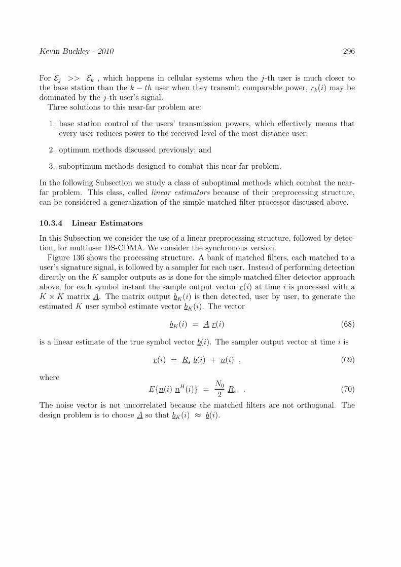
Kevin Buckley - 2010 296
For Ej >> Ek , which happens in cellular systems when the j-th user is much closer tothe base station than the k − th user when they transmit comparable power, rk(i) may bedominated by the j-th user’s signal.
Three solutions to this near-far problem are:
1. base station control of the users’ transmission powers, which effectively means thatevery user reduces power to the received level of the most distance user;
2. optimum methods discussed previously; and
3. suboptimum methods designed to combat this near-far problem.
In the following Subsection we study a class of suboptimal methods which combat the near-far problem. This class, called linear estimators because of their preprocessing structure,can be considered a generalization of the simple matched filter processor discussed above.
10.3.4 Linear Estimators
In this Subsection we consider the use of a linear preprocessing structure, followed by detec-tion, for multiuser DS-CDMA. We consider the synchronous version.
Figure 136 shows the processing structure. A bank of matched filters, each matched to auser’s signature signal, is followed by a sampler for each user. Instead of performing detectiondirectly on the K sampler outputs as is done for the simple matched filter detector approachabove, for each symbol instant the sample output vector r(i) at time i is processed with aK × K matrix A. The matrix output bK(i) is then detected, user by user, to generate theestimated K user symbol estimate vector bK(i). The vector
bK(i) = A r(i) (68)
is a linear estimate of the true symbol vector b(i). The sampler output vector at time i is
r(i) = Rs b(i) + n(i) , (69)
where
En(i) nH(i) =N0
2Rs . (70)
The noise vector is not uncorrelated because the matched filters are not orthogonal. Thedesign problem is to choose A so that bK(i) ≈ b(i).

Kevin Buckley - 2010 297
i Tb
g (T −t)b1
g (T −t)b2
g (T −t)bK
r (i) A
b (i)^1
b (i)2
b (i)K
r(t)
......
......
......
Figure 136: The linear receiver for asynchronous multiuser CDMA.
An Unbiased Estimator (i.e. the decorrelating detector)
Here we design A so that EbK(i) = b(i). Since
bK(i) = A r(i) = A [Rsb + n(i)] , (71)
we have thatEbK(i) = A Rs b(i) + EA n(i) . (72)
The noise term is zero since the noise is zero mean (by assumption). So for
Ao = R−1s (73)
we have that EbK(i) = b(i). Thus, (73) is the solution to the unbiased estimator problem.Using Ao, we have that the input to the detector is
boK(i) = Ao r(i) = b(i) + R−1
s n(i) . (74)
The estimate of a user’s symbol is decorrelated with the other users’ symbols, but the noiseterm R−1
s n(i) can be a problem. Often the unbiased estimator design approach is not thebest.

Kevin Buckley - 2010 298
The MMSE Detector
Now, design A according to the following optimization problem:
minA
E ||b(i) − bK(i)||2 , (75)
where bK(i) = A r(i). The equivalent problem, after noise whitening as illustrated below,is
minA
′
E ||b(i) − A′
r′
(i)||2 . (76)
The optimum solution is,A
′o = R−1P (77)
where R = Er′
(i) r′H(i) = Rs + N0
2IK and P = Er
′
(i) bH(i) = R1/2s . So,
A′o =
(
Rs +N0
2IK
)−1
R1/2s (78)
and
Ao = A′o R−1/2
s =(
Rs +N0
2IK
)−1
. (79)
Finally,
boK(i) =
(
Rs +N0
2IK
)−1
r(i) . (80)
r (i) b (i)K
r (i)’
A’R s
−1/2
Figure 137: The linear MMSE detector for synchronous multiuser CDMA.