ece 5424:#introduction#to# machine#learningf16ece5424/slides/l12...ece 5424:#introduction#to#...
TRANSCRIPT

ECE 5424: Introduction to Machine Learning
Stefan LeeVirginia Tech
Topics: – Classification: Logistic Regression– NB & LR connections
Readings: Barber 17.4

Administrativia• HW1 Graded
(C) Dhruv Batra 2

Administrativia• HW2
– Due: Monday, 10/3, 11:55pm– Implement linear regression, Naïve Bayes, Logistic Regression
• Review Lecture Tues
• Midterm Thursday– In class, class timing, open notes/book– Closed internet
(C) Dhruv Batra 3

Recap of last time
(C) Dhruv Batra 4

Naïve Bayes (your first probabilistic classifier)
(C) Dhruv Batra 5
Classificationx y Discrete

Classification• Learn: h:X! Y
– X – features– Y – target classes
• Suppose you know P(Y|X) exactly, how should you classify?– Bayes classifier:
• Why?
Slide Credit: Carlos Guestrin

Error Decomposition• Approximation/Modeling Error
– You approximated reality with model
• Estimation Error– You tried to learn model with finite data
• Optimization Error– You were lazy and couldn’t/didn’t optimize to completion
• Bayes Error– Reality just sucks– http://psych.hanover.edu/JavaTest/SDT/ROC.html
(C) Dhruv Batra 7

Generative vs. Discriminative
• Generative Approach (Naïve Bayes)– Estimate p(x|y) and p(y)– Use Bayes Rule to predict y
• Discriminative Approach– Estimate p(y|x) directly (Logistic Regression)– Learn “discriminant” function h(x) (Support Vector Machine)
(C) Dhruv Batra 8

The Naïve Bayes assumption• Naïve Bayes assumption:
– Features are independent given class:
– More generally:
• How many parameters now?• Suppose X is composed of d binary features
Slide Credit: Carlos Guestrin(C) Dhruv Batra 9
d

Generative vs. Discriminative
• Generative Approach (Naïve Bayes)– Estimate p(x|y) and p(y)– Use Bayes Rule to predict y
• Discriminative Approach– Estimate p(y|x) directly (Logistic Regression)– Learn “discriminant” function h(x) (Support Vector Machine)
(C) Dhruv Batra 10

Today: Logistic Regression• Main idea
– Think about a 2 class problem {0,1}– Can we regress to P(Y=1 | X=x)?
• Meet the Logistic or Sigmoid function– Crunches real numbers down to 0-1
• Model– In regression: y ~ N(w’x, λ2)– Logistic Regression: y ~ Bernoulli(σ(w’x))
(C) Dhruv Batra 11
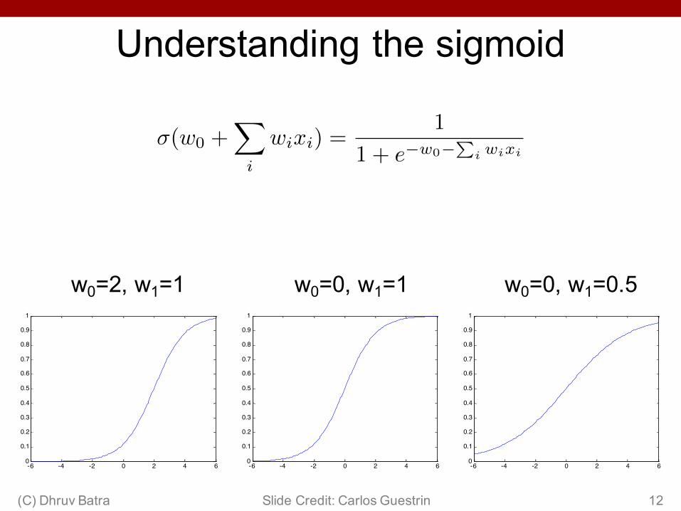
Understanding the sigmoid
-6 -4 -2 0 2 4 60
0.1
0.2
0.3
0.4
0.5
0.6
0.7
0.8
0.9
1
w0=0, w1=1
-6 -4 -2 0 2 4 60
0.1
0.2
0.3
0.4
0.5
0.6
0.7
0.8
0.9
1
w0=2, w1=1
-6 -4 -2 0 2 4 60
0.1
0.2
0.3
0.4
0.5
0.6
0.7
0.8
0.9
1
w0=0, w1=0.5
Slide Credit: Carlos Guestrin(C) Dhruv Batra 12
�(w0 +X
i
wi
xi
) =1
1 + e�w0�P
i wixi

Visualization
(C) Dhruv Batra 13
−3 −2 −1 0 1 2 3 4 5 6
−3
−2
−1
0
1
2
3
4
5
−100
10 −100
100
0.5
1
x2
W = ( −2 , −1 )
x1
−100
10 −100
100
0.5
1
x2
W = ( −2 , 3 )
x1−10
010 −10
010
0
0.5
1
x2
W = ( 0 , 2 )
x1
−100
10 −100
100
0.5
1
x2
W = ( 1 , 4 )
x1
−100
10 −100
100
0.5
1
x2
W = ( 1 , 0 )
x1
−100
10 −100
100
0.5
1
x2
W = ( 2 , 2 )
x1
−100
10 −100
100
0.5
1
x2
W = ( 2 , −2 )
x1
−100
10 −100
100
0.5
1
x2
W = ( 3 , 0 )
x1
−100
10 −100
100
0.5
1
x2
W = ( 5 , 4 )
x1
−100
10 −100
100
0.5
1
x2
W = ( 5 , 1 )
x1
w1
w2
Slide Credit: Kevin Murphy

Expressing Conditional Log Likelihood
Slide Credit: Carlos Guestrin(C) Dhruv Batra 14
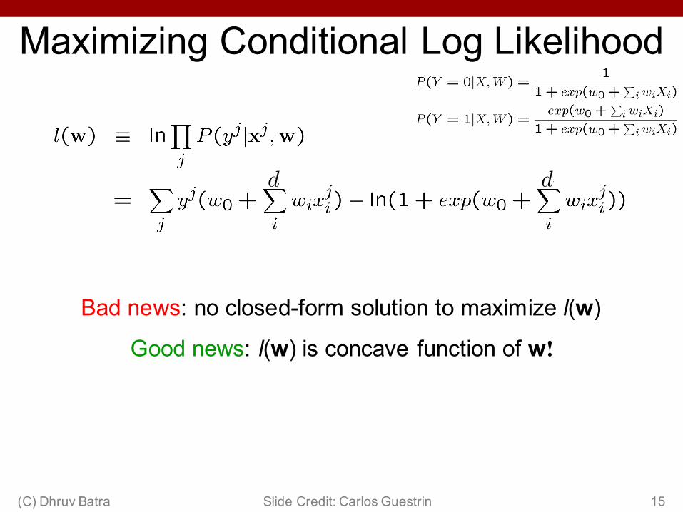
Maximizing Conditional Log Likelihood
Bad news: no closed-form solution to maximize l(w)
Good news: l(w) is concave function of w!
Slide Credit: Carlos Guestrin(C) Dhruv Batra 15
dd
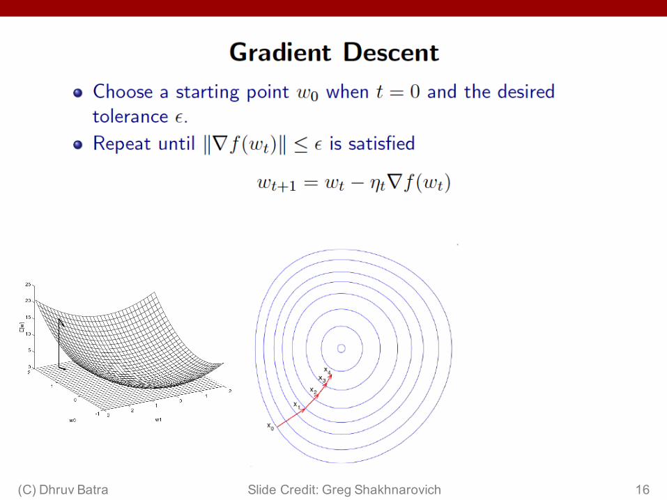
(C) Dhruv Batra 16Slide Credit: Greg Shakhnarovich

Careful about step-size
(C) Dhruv Batra 17Slide Credit: Nicolas Le Roux

(C) Dhruv Batra 18Slide Credit: Fei Sha

When does it work?
(C) Dhruv Batra 19
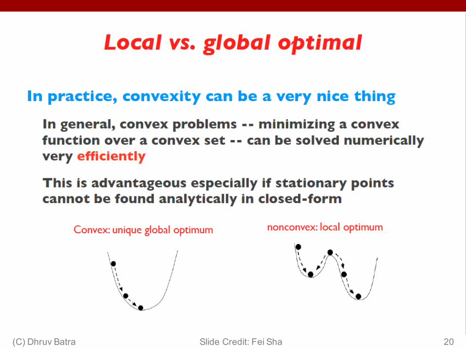
(C) Dhruv Batra 20Slide Credit: Fei Sha

(C) Dhruv Batra 21Slide Credit: Greg Shakhnarovich
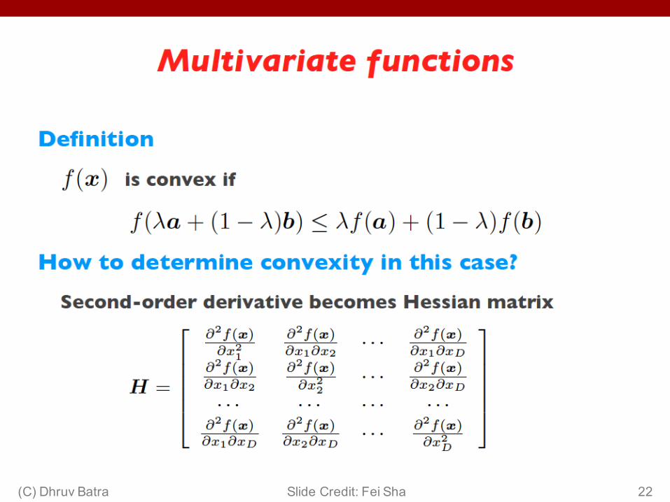
(C) Dhruv Batra 22Slide Credit: Fei Sha
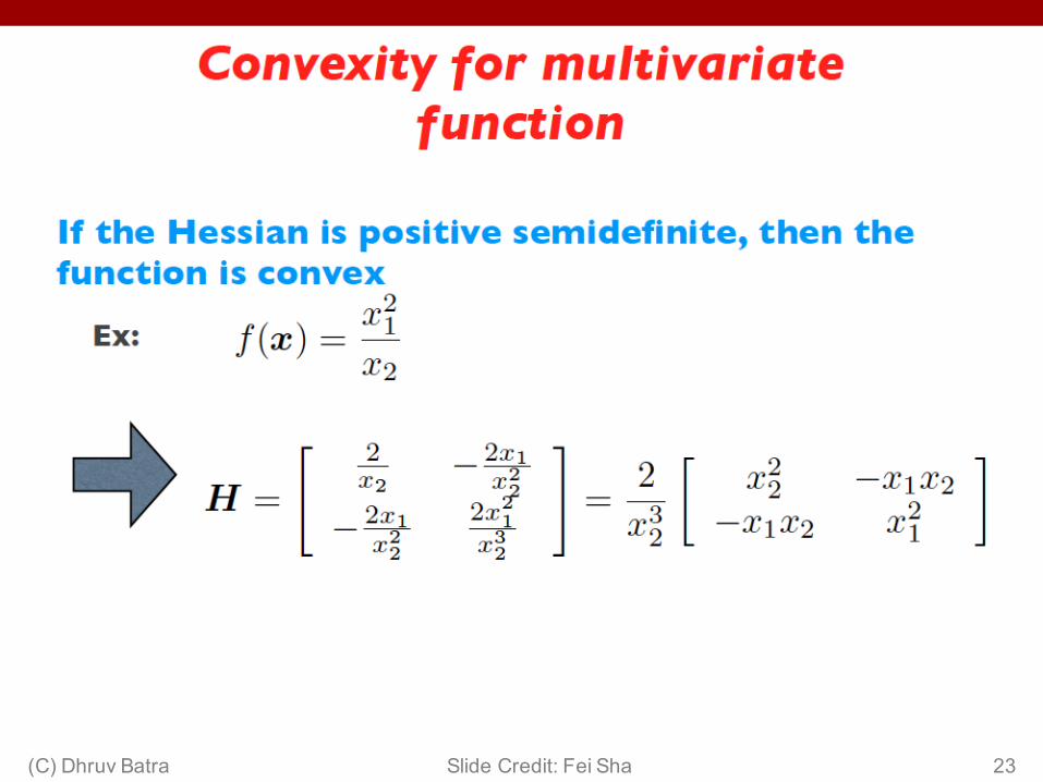
(C) Dhruv Batra 23Slide Credit: Fei Sha
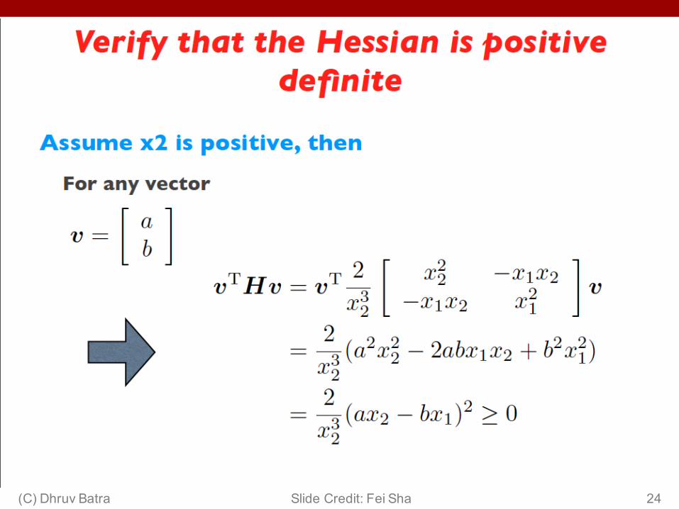
(C) Dhruv Batra 24Slide Credit: Fei Sha

(C) Dhruv Batra 25Slide Credit: Fei Sha

Optimizing concave function –Gradient ascent
• Conditional likelihood for Logistic Regression is concaveà Find optimum with gradient ascent
Gradient:
Learning rate, �>0
Update rule:
Slide Credit: Carlos Guestrin(C) Dhruv Batra 26

Slide Credit: Carlos Guestrin(C) Dhruv Batra 27
dd
Maximize Conditional Log Likelihood: Gradient ascent
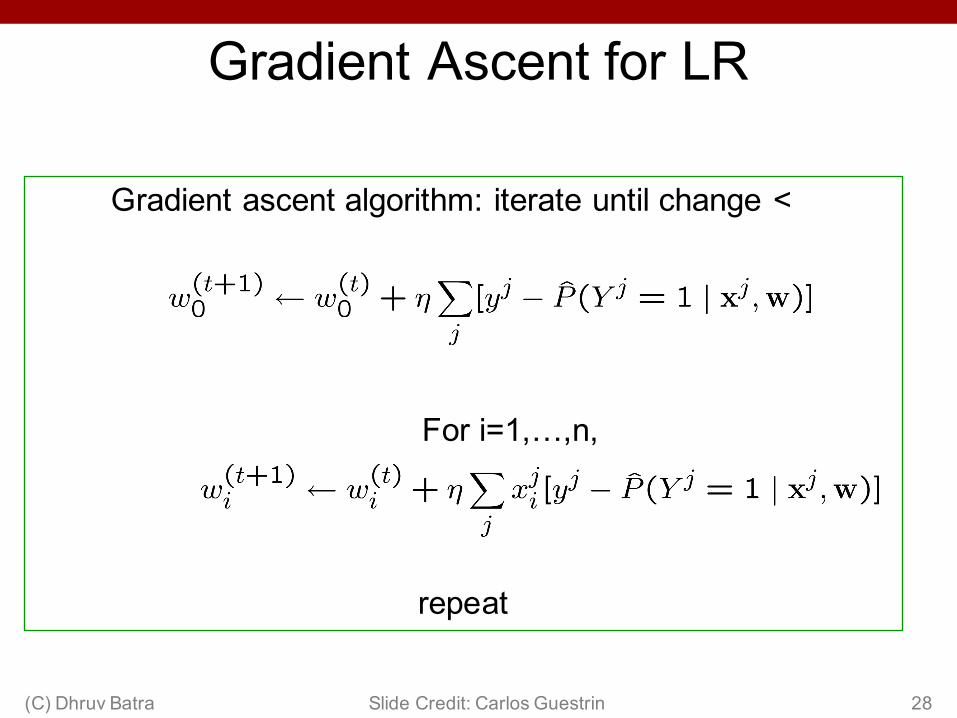
Gradient Ascent for LR
Gradient ascent algorithm: iterate until change < �
For i=1,…,n,
repeat
Slide Credit: Carlos Guestrin(C) Dhruv Batra 28

(C) Dhruv Batra 29

That’s all M(C)LE. How about M(C)AP?
• One common approach is to define priors on w– Normal distribution, zero mean, identity covariance– “Pushes” parameters towards zero
• Corresponds to Regularization– Helps avoid very large weights and overfitting– More on this later in the semester
• MAP estimate
Slide Credit: Carlos Guestrin(C) Dhruv Batra 30

Large parameters � Overfitting
• If data is linearly separable, weights go to infinity• Leads to overfitting
• Penalizing high weights can prevent overfitting
Slide Credit: Carlos Guestrin(C) Dhruv Batra 31

Gradient of M(C)AP
Slide Credit: Carlos Guestrin(C) Dhruv Batra 32

MLE vs MAP
• Maximum conditional likelihood estimate
• Maximum conditional a posteriori estimate
Slide Credit: Carlos Guestrin(C) Dhruv Batra 33

HW2 Tips• Naïve Bayes
– Train_NB• Implement “factor_tables” -- |Xi| x |Y| matrices• Prior |Y| x 1 vector• Fill entries by counting + smoothing
– Test_NB• argmax_y P(Y=y) P(Xi=xi)…
– TIP: work in log domain
• Logistic Regression– Use small step-size at first– Make sure you maximize log-likelihood not minimize it– Sanity check: plot objective
(C) Dhruv Batra 34
Finishing up: Connections between NB & LR
(C) Dhruv Batra 35

Logistic regression vs Naïve Bayes• Consider learning f: X à Y, where
– X is a vector of real-valued features, <X1 … Xd>– Y is boolean
• Gaussian Naïve Bayes classifier– assume all Xi are conditionally independent given Y– model P(Xi | Y = k) as Gaussian N(�ik,�i)– model P(Y) as Bernoulli(θ,1-θ)
• What does that imply about the form of P(Y|X)?
Slide Credit: Carlos Guestrin 36(C) Dhruv Batra Cool!!!!
P (Y = 1 | X = x) =1
1 + exp(�w0 �P
i wixi)

Derive form for P(Y|X) for continuous Xi
Slide Credit: Carlos Guestrin 37(C) Dhruv Batra
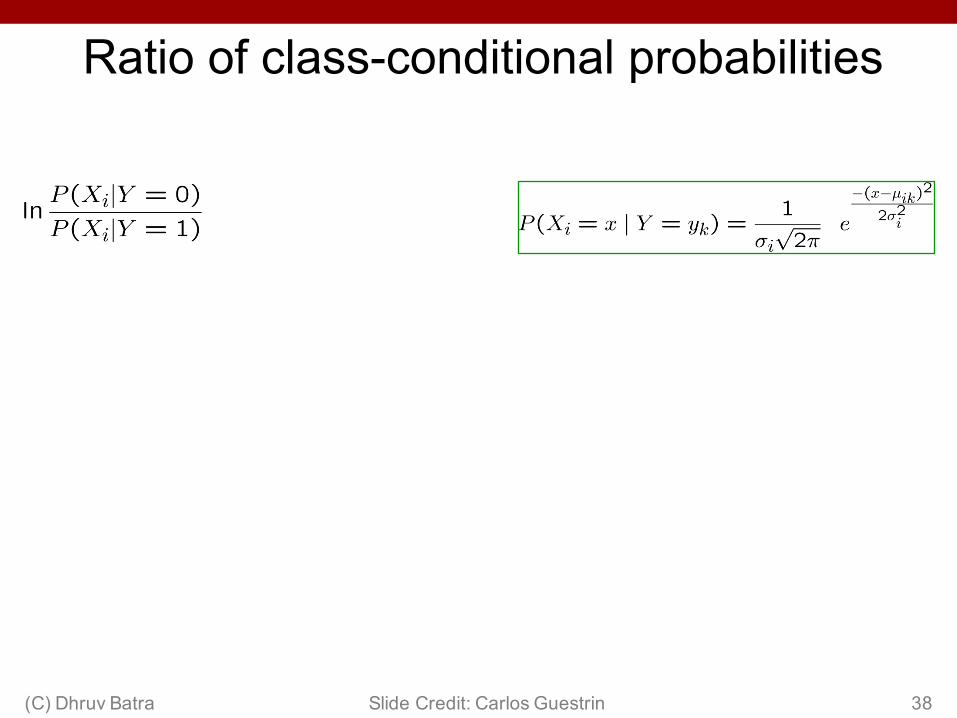
Ratio of class-conditional probabilities
Slide Credit: Carlos Guestrin 38(C) Dhruv Batra

Derive form for P(Y|X) for continuous Xi
Slide Credit: Carlos Guestrin 39(C) Dhruv Batra
P (Y = 1 | X = x) =1
1 + exp(�w0 �P
i wixi)

Gaussian Naïve Bayes vs Logistic Regression
• Representation equivalence– But only in a special case!!! (GNB with class-independent variances)
• But what’s the difference???• LR makes no assumptions about P(X|Y) in learning!!!• Loss function!!!
– Optimize different functionsà Obtain different solutions
Set of Gaussian Naïve Bayes parameters
(feature variance independent of class label)
Set of Logistic Regression parameters
Slide Credit: Carlos Guestrin 40(C) Dhruv Batra
Not necessarily

Naïve Bayes vs Logistic Regression
Slide Credit: Carlos Guestrin 41(C) Dhruv Batra
Consider Y boolean, Xi continuous, X=<X1 ... Xd>
• Number of parameters:– NB: 4d +1 (or 3d+1)– LR: d+1
• Estimation method:– NB parameter estimates are uncoupled– LR parameter estimates are coupled

[Ng & Jordan, 2002]
Slide Credit: Carlos Guestrin 42(C) Dhruv Batra
• Generative and Discriminative classifiers
• Asymptotic comparison (# training examples à infinity)
– when model correct• GNB (with class independent variances) and LR produce identical classifiers
– when model incorrect• LR is less biased – does not assume conditional independence
– therefore LR expected to outperform GNB
G. Naïve Bayes vs. Logistic Regression 1

[Ng & Jordan, 2002]
Slide Credit: Carlos Guestrin 43(C) Dhruv Batra
G. Naïve Bayes vs. Logistic Regression 2• Generative and Discriminative classifiers
• Non-asymptotic analysis– convergence rate of parameter estimates, d = # of attributes in X• Size of training data to get close to infinite data solution• GNB needs O(log d) samples• LR needs O(d) samples
– GNB converges more quickly to its (perhaps less helpful) asymptotic estimates

Some experiments from UCI data
sets
Naïve bayes
Logistic Regression
(C) Dhruv Batra

• Gaussian Naïve Bayes with class-independent variances representationally equivalent to LR– Solution differs because of objective (loss) function
• In general, NB and LR make different assumptions– NB: Features independent given class assumption on P(X|Y)– LR: Functional form of P(Y|X), no assumption on P(X|Y)
• LR is a linear classifier– decision rule is a hyperplane
• LR optimized by conditional likelihood– no closed-form solution– Concave à global optimum with gradient ascent– Maximum conditional a posteriori corresponds to regularization
• Convergence rates– GNB (usually) needs less data– LR (usually) gets to better solutions in the limit
(C) Dhruv Batra 45Slide Credit: Carlos Guestrin
What you should know about LR