ec202 slides lecture 3

8/11/2019 EC202 Slides Lecture 3

http://slidepdf.com/reader/full/ec202-slides-lecture-3 1/43

EC202 Microeconomic Principles II: Lecture 3

Leonardo Felli

CLM.G.02

30 January 2014



Static Bayesian Games

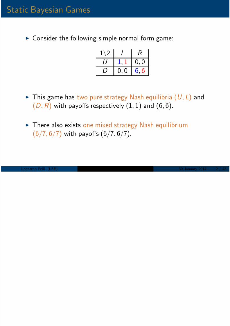
Consider the following simple normal form game:

1\2 L R

U 1, 1 0, 0

D 0, 0 6, 6

This game has two pure strategy Nash equilibria (U , L) and(D , R ) with payoffs respectively (1, 1) and (6, 6).

There also exists one mixed strategy Nash equilibrium(6/7, 6/7) with payoffs (6/7, 6/7).

Leonardo Felli (LSE) EC202 Microeconomic Principles II 30 January 2014 2 / 43



Static Bayesian Game: Example

Assume now that player 2 has some ‘small’ uncertainty when

casting her choice of strategy in the game. With probability

9

10 she thinks she is playing Game A:

1\2 L R

U A 1, 1 0, 0D A 0, 0 6, 6

while with probability 1

10 she thinks she is playing Game B:

1\2 L R

U B 1, 0 0, 10

D B 0, 0 6, 6




Static Bayesian Games: Assumptions

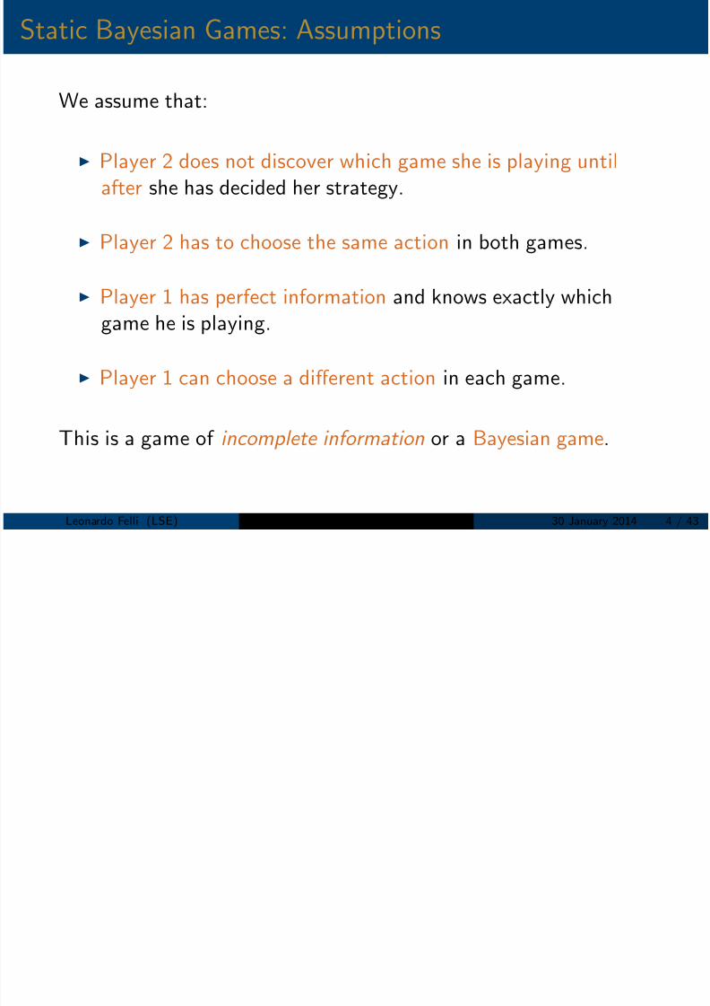
We assume that:

Player 2 does not discover which game she is playing untilafter she has decided her strategy.

Player 2 has to choose the same action in both games.

Player 1 has perfect information and knows exactly whichgame he is playing.

Player 1 can choose a different action in each game.

This is a game of incomplete information or a Bayesian game.




Static Bayesian Games: Player 1’s Strategies

This is a simultaneous move game hence Nash equilibrium

should be the basic tool to get a prediction.

We can than determine the strategy choice of player 1 as afunction of what he expects player 2 to do as best reply.

As argued above, a strategy choice for player 1 is a pair of actions,

(aA, aB )

the first element specifies the action player 1 will take if the

game is A: aA,

the second element specifies the action player 1 will take if thegame is B: aB .




Static Bayesian Games: Player 1’s Best Reply

1\2.A L R 1\2.B L R U A 1,1 0,0 U B 1,0 0,10D A 0,0 6,6 D B 0,0 6,6

If the game played is A then player 1’s best reply if he expects

player 2 to play L is U A, while his best reply if he expectsplayer 2 to play R is D A.

If the game played is B then player 1’s best reply if he expectsplayer 2 to play L is U B , while his best reply if he expects

player 2 to play R is D B .

This is not a surprise since the payoffs to player 1 are the same inboth games.




Static Bayesian Games: Player 2’s Strategies

To be able to determine player 2 best reply however strategies

and payoffs are not enough.

We need to take into account player 2’s beliefs about whichgame is played.

As mentioned in the description of the game player 2 believesthat:

with probability 9/10 the game played is A,

with probability 1/10 the game played is B.

We then need to compute player 2’s expected payoffs in thegame given her beliefs on which game is played.





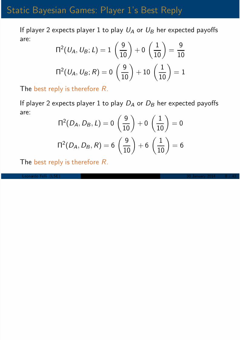
If player 2 expects player 1 to play U A or U B her expected payoffs

are:Π2(U A, U B ; L) = 1

9

10

+ 0

1

10

=

9

10

Π2(U A, U B ; R ) = 0

9

10

+ 10

1

10

= 1

The best reply is therefore R .

If player 2 expects player 1 to play D A or D B her expected payoffsare:

Π

2

(D A, D B , L) = 0 9

10

+ 0 1

10

= 0

Π2(D A, D B , R ) = 6

9

10

+ 6

1

10

= 6

The best reply is therefore R .





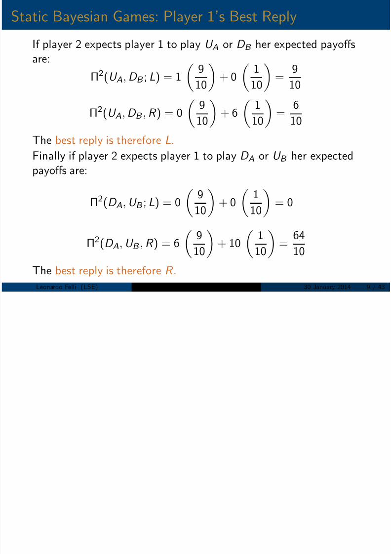
If player 2 expects player 1 to play U A or D B her expected payoffsare:

Π2(U A, D B ; L) = 1

910

+ 0

110

= 9

10

Π2(U A, D B , R ) = 0

9

10

+ 6

1

10

=

6

10

The best reply is therefore L.Finally if player 2 expects player 1 to play D A or U B her expectedpayoffs are:

Π2

(D A, U B ; L) = 0 9

10

+ 0 1

10

= 0

Π2(D A, U B , R ) = 6

9

10

+ 10

1

10

=

64

10

The best reply is therefore R .Leonardo Felli (LSE) EC202 Microeconomic Principles II 30 January 2014 9 / 43



Static Bayesian Games: Bayesian Nash Equilibrium

Recall that player 1’s best reply is:

if player 2 chooses L to play U A and U B ,

if player 2 chooses R to play D A and D B .

The unique Bayesian Nash equilibrium of the game is therefore:

player 2 chooses R and

player 1 chooses D A if the game is A and D B if the game is B.

The equilibrium payoffs for the two players are:

π1A(D A, D B , R ) = 6, π1

B (D A, D B , R ) = 6, Π2(D A, D B , R ) = 6.




Incomplete Information (Strategic Form)

An incomplete information game consists of:

N the set of players in the game

Ai player i ’s action set

Ti player i ’s set of possible types

A profile of types t = (t 1,..., t n) is an element T = × j ∈N T j

µ a distribution over the possible types

u i : A × T → R player i ’s utility function, u i (a|t )




Bayesian Game Example

Consider the Bayesian game we solved before:

Player 1’s type takes two values: T1 = {A, B}

Player 2’s type takes only one values: T2 = {C }

Probabilities are such that: µ(C , A) = 0.9

Payoffs and action sets are as described in the matrix:

1\2.A L R 1\2.B L R

U A 1,1 0,0 U B 1,0 0,10D A 0,0 6,6 D B 0,0 6,6




Information Structure

Information structure:

T i denotes the type as a random variable

its realizations belong to the set of possible types Ti

t i denotes the realization of the random variable T i

T −i = (T 1, ..., T i −1, T i +1, ..., T n) denotes a profile of types forall players other than i

Player i observes only the realization of T i

Player i ignores T −i , but knows µi

Player i has beliefs regarding the realization of the types of theother players t −i




Beliefs about other Players’ Types [Take 1]

In this course we consider models in which types are independent:

µ(t ) = j ∈N

µ j (t j )

This implies that the type T i of player i is independent of T −i

Beliefs are a probability distribution over the types of the otherplayers

Any player forms beliefs about the types of the other players byusing Bayes Rule

Independence implies that conditional on observing T i = t i thebeliefs of player i are:

µi (t −i |t i ) =

j ∈N \i

µ j (t j ) = µ−i (t −i )




Extra: Beliefs about other Players’ Types [Take 2]

Also in the general case with interdependence players form beliefs

about the types received by the others by using Bayes Rule

Conditional observing T i = t i the beliefs of player i are:

µi (t −i |t i ) = Pr(T −i = t −i |T i = t i ) =

= Pr(T −i = t −i ∩ T i = t i )

Pr(T i = t i ) =

= Pr(T −i = t −i ∩ T i = t i )

τ −i ∈T−i Pr(T −i = τ −i ∩ T i = t i )

=

= µ(t −i , t i )

τ −i ∈T−i

µ(τ −i , t i )




Strategies

Strategy Profiles:

A strategy consists of a map from available information toactions:

s i : Ti → Ai

s i (T i ) specifies an action for every realization of the type T i .

A strategy profile consists of a strategy for every player:

s (T ) = (s 1(T 1), ..., s N (T N ))

We adopt the usual convention:

s −i (T −i ) = (s 1(T 1), ..., s i −1(T i −1), s i +1(T i +1), ..., s N (T N ))


B i G E l ( ’d)



Bayesian Game Example (cont’d)

Consider the Bayesian game we solved before:

Players’ types are: T1 = {A, B}, T2 = {C }

Probabilities are such that: µ(C , A) = 0.9

Payoffs and action sets are as described in the matrix:

1\2.A L R 1\2.B L R

U A 1,1 0,0 U B 1,0 0,10D A 0,0 6,6 D B 0,0 6,6

A strategy for player 1 is a map s 1 : {A, B } → {U , D }, it is apair (aA, aB )

A strategy for player 2 is an element of the set s 2 ∈ {L, R }

Player 2 cannot act upon player 1’s private information


D i S E ilib i



Dominant Strategy Equilibrium

Strategy s i weakly dominates s i if for any a−i and t ∈ T:

u i (s i (t i ), a−i |t ) ≥ u i (s i (t i ), a−i |t ) with > for some a−i

Strategy s i is dominant if it dominates any other strategy s i

Strategy s i is undominated if no strategy dominates it

Definitions (Dominant Strategy Equilibrium DSE)

A Dominant Strategy equilibrium of an incomplete informationgame is a strategy profile s that for any i ∈ N , t ∈ T and

a−i ∈ A−i satisfies:

u i (s i (t i ), a−i |t ) ≥ u i (s i (t i ), a−i |t ) for any s i : Ti → Ai

I.e. s i is optimal independently of what others know and do


I i E d U ili



Interim Expected Utility

The interim stage occurs just after a player knows his type

T i = t i

It is when strategies are chosen in a Bayesian game

The interim expected utility of a (pure) strategy profile s isdefined by:

U i (s |t i ) =T−i

u i (s (t )|t )µ(t −i |t i ) : Ti → R

With such notation in mind notice that:

U i (ai , s −i |t i ) =T−i

u i (ai , s −i (t −i )|t )µ(t −i |t i )


B t R l



Best Reply

The best reply correspondence of player i is defined by:

bi (s −i |t i ) = arg maxai ∈Ai

U i (ai , s −i |t i )

BR maps identify which actions are optimal given the typeobserved by player i and the strategies followed by the otherplayers −i .


P St t B N h E ilib i



Pure Strategy Bayes Nash Equilibrium

Definitions (Bayes Nash Equilibrium BNE)A pure strategy Bayes Nash equilibrium of an incompleteinformation game is a strategy profile s such that for any i ∈ N

and t i ∈ Ti satisfies:

U i (s |t i ) ≥ U i (ai , s −i |t i ) for any ai ∈ Ai

BNE requires interim optimality (i.e. do your best given what you

know)

BNE requires s i (t i ) ∈ bi (s −i |t i ) for any i ∈ N and t i ∈ Ti





Bayesian Game Example (cont d)

Consider the Bayesian game with µ(C , A) = 0.9:

1\2.A L R 1\2.B L R

U A 1,1 0,0 U B 1,0 0,10D A 0,0 6,6 D B 0,0 6,6

As seen above the best reply maps for both player are:

b1(s 2|A) =

U A if s 2 = L

D A if s 2 = R b1(s 2|B ) =

U B if s 2 = L

D B if s 2 = R

whileb2(s 1) =

L if s 1 = (U A, D B )R otherwise





Bayesian Game Example (cont d)

As seen above, this Bayesian game has a unique (pure strategy)BNE in which:

s 1(A) = D A, s 1(B ) = D B , s 2 = R

The payoffs associated with the BNE are:

U 1(D A, D B , R |A) = 6,

U 1(D A, D B , R |B ) = 6,

U 2(D A, D B , R ) = 6.

DO NOT ANALYZE MATRICES SEPARATELY!!!


Relationships between Equilibrium Concepts



DSE Example: Exchange

A buyer and a seller want to trade an object:

Buyer’s value for the object is £3

Seller’s value is either £0 or £2 based on its type,TS = {L, H }. The buyer does not observe this.

Buyer can offer either £1 or £3 to purchase the object

Seller decides whether or not to sell.


DSE Example: Exchange (cont’d)



DSE Example: Exchange (cont d)

The game is described by the following matrixes:

B \S .L sale no sale B \S .H sale no sale

£3 0,3 0,0 £3 0,1 0,2£1 2,1 0,0 £1 2,-1 0,2

This game for any B’s beliefs 0 < µ < 1 has a DSE in which:

σS (L) = sale, σS (H ) = no sale, σB = £1where σi (t i ) is player i ’s strategy if the type is t i .

Offering £1 is a weakly dominant strategy for the buyer:whatever σS

U B (£1, σS ) ≥ U B (£3, σS ) = 0

Once S expects B to offer £1 then it is optimal for S tochoose “sale” if t S = L and “no sale” if t S = H .


Static Bayesian Games: Cournot Duopoly



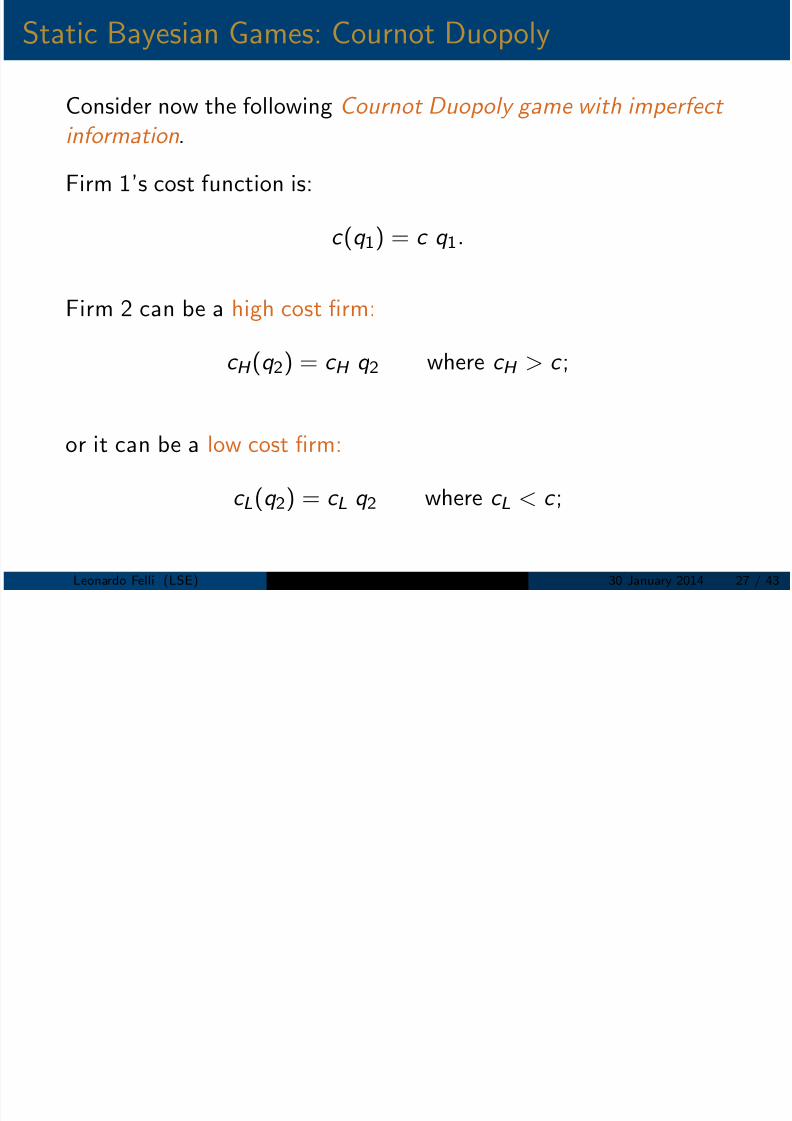
Static Bayesian Games: Cournot Duopoly

Consider now the following Cournot Duopoly game with imperfect

information.Firm 1’s cost function is:

c (q 1) = c q 1.

Firm 2 can be a high cost firm:

c H (q 2) = c H q 2 where c H > c ;

or it can be a low cost firm:

c L(q 2) = c L q 2 where c L < c ;


Static Bayesian Games: Cournot Duopoly (cont’d)



Static Bayesian Games: Cournot Duopoly (cont d)

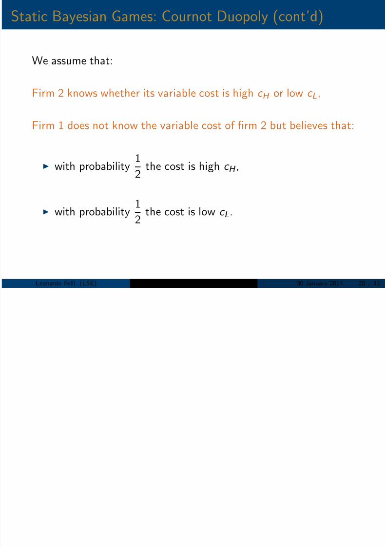
We assume that:

Firm 2 knows whether its variable cost is high c H or low c L,

Firm 1 does not know the variable cost of firm 2 but believes that:

with probability 1

2 the cost is high c H ,

with probability 12

the cost is low c L.






The inverse demand function faced by both firms is:

P (q 1 + q 2) = a − (q 1 + q 2)

where c H < a.

Notice that firm 1 will choose a unique quantity.

Notice that firm 2 will choose a different quantity depending onwhether its cost is high or low.

We label these quantities: q H 2 or q L2 .






Depending on the value of the cost firm 2’s profit functions are:

ΠH 2 (q 1, q H 2 ) = q H 2

a − (q 1 + q H 2 ) − c H

orΠL

2(q 1, q L2 ) = q L2 a − (q 1 + q L2 ) − c Lwhile firm 1’s expected profit function is:

Π1

(q 1

, q H

2 , q L

2) =

1

2 q

1a − (q

1 + q H

2 ) − c +

+ 1

2 q 1

a − (q 1 + q L2 ) − c






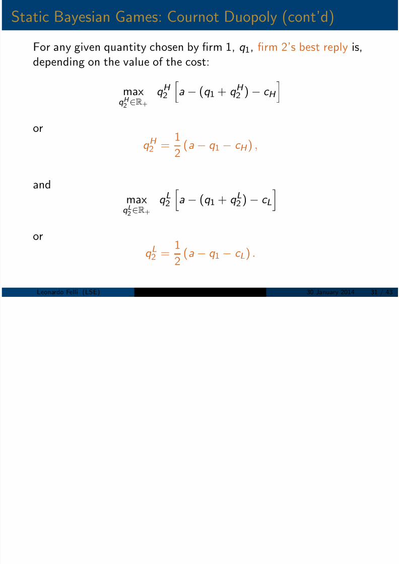
For any given quantity chosen by firm 1, q 1, firm 2’s best reply is,depending on the value of the cost:

maxq H 2 ∈R+

q H 2

a − (q 1 + q H 2 ) − c H

or

q H 2 = 1

2 (a − q 1 − c H ) ,

andmax

q

L

2∈R

+

q L2 a − (q 1 + q L2 ) − c Lor

q L2 = 1

2 (a − q 1 − c L) .





y p y ( )

For any given quantity chosen by the two types of firm 2 q H 2 and

q L2 , firm 1’s best reply is:

maxq 1∈R+

1

2 q 1 a − (q 1 + q H

2 ) − c +

1

2 q 1 a − (q 1 + q L

2) − c

or

q 1 = 1

2

1

2

a − q H 2 − c

+

1

2

a − q L2 − c

.





y p y ( )

In other words the best reply of the two types of firm 2 and of firm

1 are:

q H 2 = 1

2 (a − q 1 − c H ) ,

q L2 = 1

2 (a − q 1 − c L) ,

q 1 = 1

2

1

2

a − q H 2 − c

+

1

2

a − q L2 − c

.





y p y ( )

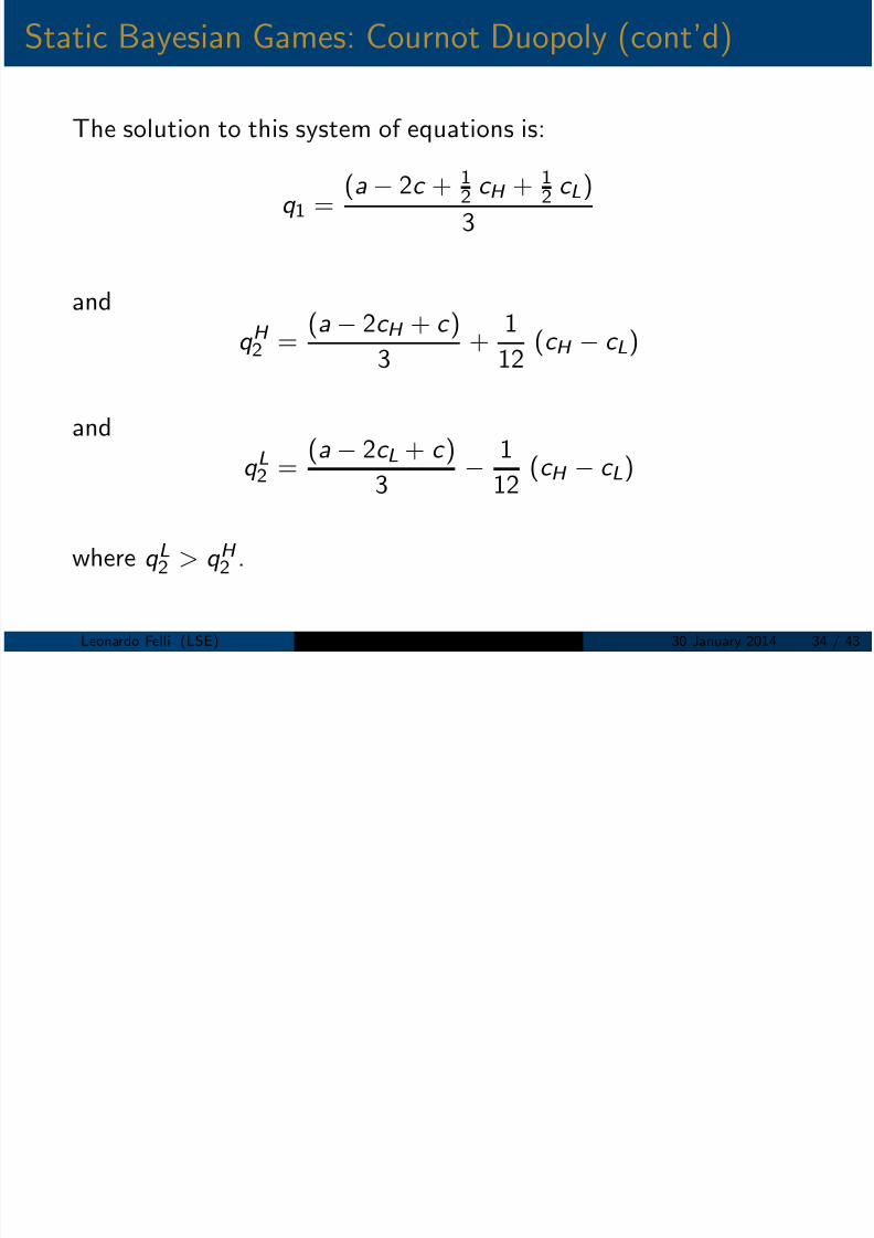
The solution to this system of equations is:

q 1 = (a − 2c + 1

2 c H + 12 c L)

3

and

q H 2 = (a − 2c H + c )3

+ 112

(c H − c L)

and

q L2 =

(a − 2c L + c )

3 − 1

12 (c H − c L)

where q L2 > q H 2 .





y p y ( )

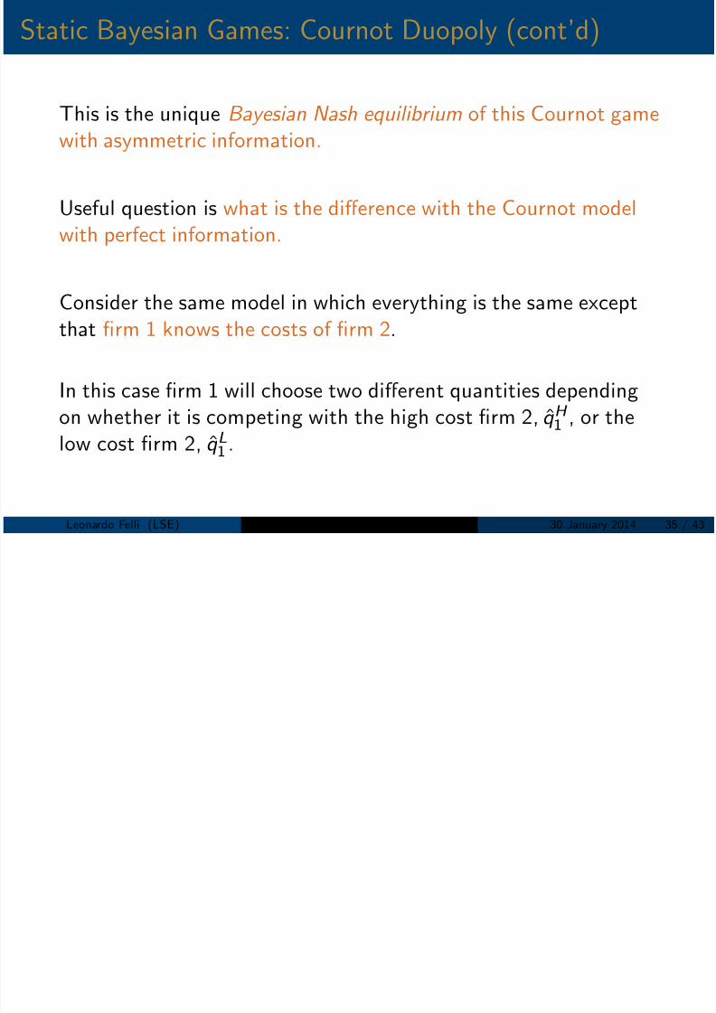
This is the unique Bayesian Nash equilibrium of this Cournot game

with asymmetric information.

Useful question is what is the difference with the Cournot modelwith perfect information.

Consider the same model in which everything is the same exceptthat firm 1 knows the costs of firm 2.

In this case firm 1 will choose two different quantities dependingon whether it is competing with the high cost firm 2, q̂ H 1 , or thelow cost firm 2, q̂ L1 .





( )

These quantities are the solution to the following two problems:

maxq̂ H 1 ∈R+

q̂ H 1

a − (q̂ H 1 + q̂ H 2 ) − c

with best reply:

q̂

H

1 =

1

2

a − q̂

H

2 − c

,

andmaxq̂ L1∈R+

q̂ L1

a − (q̂ L1 + q̂ L2 ) − c L

or

q̂ L1 = 1

2

a − q̂ L2 − c

.





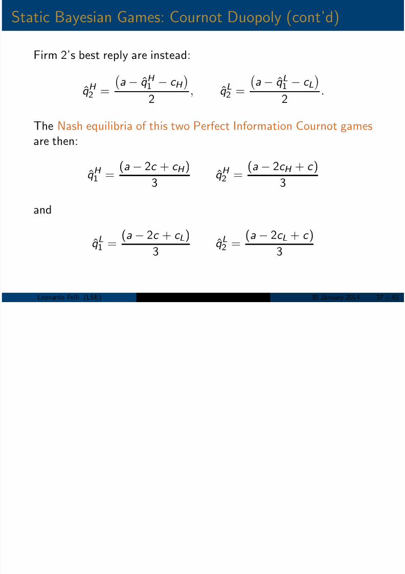
Firm 2’s best reply are instead:

q̂ H 2 =

a − q̂ H 1 − c H

2

, q̂ L2 =

a − q̂ L1 − c L

2

.

The Nash equilibria of this two Perfect Information Cournot games

are then:

q̂ H 1 = (a − 2c + c H )

3 q̂ H 2 =

(a − 2c H + c )

3

and

q̂ L1 = (a − 2c + c L)

3 q̂ L2 =

(a − 2c L + c )

3





Compare now the quantities chosen by firm 2 in the presence of complete vs. asymmetric information:

q H 2 = (a − 2c H + c )

3 +

1

12 (c H − c L) > q̂ H 2

andq L2 =

(a − 2c L + c )

3 −

1

12 (c H − c L) < q̂ L2

while for firm 1:

q 1 =

1

2 q̂ H

1 +

1

2 q̂ L

1

orq̂ H 1 > q 1 > q̂ L1


Mixed Strategies in Bayesian Games



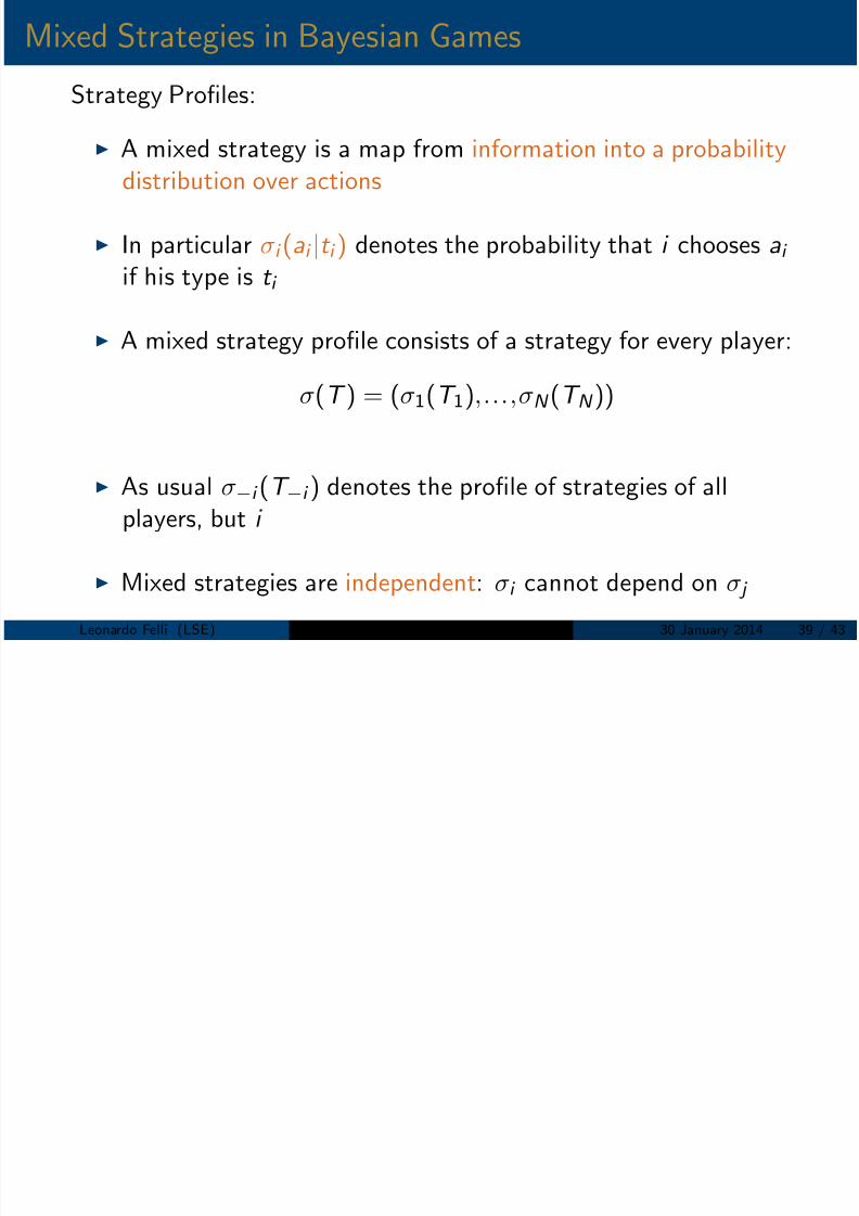
Strategy Profiles:

A mixed strategy is a map from information into a probabilitydistribution over actions

In particular σi (ai |t i ) denotes the probability that i chooses ai if his type is t i

A mixed strategy profile consists of a strategy for every player:

σ(T ) = (σ1(T 1),...,σN (T N ))

As usual σ−i (T −i ) denotes the profile of strategies of allplayers, but i

Mixed strategies are independent: σi cannot depend on σ j


Extra: Interim Payoff & Bayes Nash Equilibrium



The interim expected payoff of mixed strategy profiles σ and(ai , σ−i ) are:

U i (σ|t i ) =T−i

a∈A

u i (a|t ) j ∈N

σ j (a j |t j )µ(t −i |t i )

U i (ai , σ−i |t i ) =T−i

a−i ∈A−i

u i (a|t ) j =i

σ j (a j |t j )µ(t −i |t i )

Definitions (Bayes Nash Equilibrium BNE)

A Bayes Nash equilibrium of a game Γ is a strategy profile σ such

that for any i ∈ N and t i ∈ Ti satisfies:

U i (σ|t i ) ≥ U i (ai , σ−i |t i ) for any ai ∈ Ai

Interim optimality: do your best given what you know.Leonardo Felli (LSE) EC202 Microeconomic Principles II 30 January 2014 40 / 43

Computing Bayes Nash Equilibria



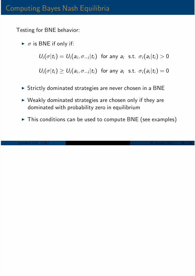
Testing for BNE behavior:

σ is BNE if only if:

U i (σ|t i ) = U i (ai , σ−i |t i ) for any ai s.t. σi (ai |t i ) > 0

U i (σ|t i ) ≥ U i (ai , σ−i |t i ) for any ai s.t. σi (ai |t i ) = 0

Strictly dominated strategies are never chosen in a BNE

Weakly dominated strategies are chosen only if they are

dominated with probability zero in equilibrium

This conditions can be used to compute BNE (see examples)


Example I



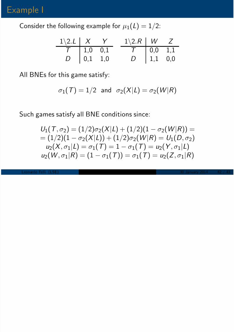
Consider the following example for µ1(L) = q ≤ 2/3:

1\2.L X Y

1\2.R W Z

T 0,0 0,2 T 2,2 0,1D 2,0 1,1 D 0,0 3,2

All BNEs for this game satisfy σ1(T ) = 2/3 and:

σ2(X |L) = 0 (dominance) and σ2(W |R ) = 3 − 2q

5 − 5q

Such games satisfy all BNE conditions since:

U 1(T , σ2) = 2(1 − q )σ2(W |R ) == q + 3(1 − q )(1 − σ2(W |R )) = U 1(D , σ2)

u 2(X , σ1|L) = 0 < 2σ1(T ) + (1 − σ1(T )) = u 2(Y , σ1|L)u 2(W , σ1|R ) = 2σ1(T ) = σ1(T ) + 2(1 − σ1(T )) = u 2(Z , σ1|R )


ec202 slides lecture 3

Documents