eba reportreport+results+from... · 1.2 portfolio composition and characteristics of institutions...
TRANSCRIPT

EBA REPORT
RESULTS FROM THE 2018 LOW AND HIGH DEFAULT PORTFOLIOS EXERCISE

RESULTS FROM THE 2018 BENCHMARKING EXERCISE
1
Contents
List of figures 3
List of tables 7
Abbreviations 8
Executive summary 11
Introduction and legal background 16
1. Section 1: General description 20
1.1 Dataset and assessment methodology 20 1.1.1 Dataset 20 1.1.2 Challenges encountered when analysing the variability of IRB models’ outcomes 21 1.1.3 Analyses performed 23
1.2 Portfolio composition and characteristics of institutions in the sample 25 1.2.1 Use of regulatory approaches 25 1.2.2 Portfolio composition and representativeness 26
2. Section 2: Quantitative analysis 34
2.1 Top-down and distribution analysis (LDPs and HDPs) 34 2.1.1 Drivers of differences in GC 35 2.1.2 Impact of the top-down analysis on the GC and RW 39 2.1.3 Key metrics 42
2.2 Analysis of IRB parameters for common counterparties (LDPs) 43 2.3 Outturns (backtesting) approaches (HDPs) 47
2.3.1 Key metrics at the risk parameters level 50
2.4 Temporal analysis 53 2.4.1 General statistics 53 2.4.2 Top-down analysis 55 2.4.3 LDP exercises 58
Comparison of the samples of counterparties 58 Comparison of the observed variability 59
2.4.4 HDP exercises 60
3. Section 3: Qualitative analysis 63
3.1 Competent authorities’ assessments 63 3.2 Results of the interviews 71 3.3 Results of the qualitative survey 72
Conclusion 82
Future work 84
Annex 1: List of participating institutions 87
Annex 2: Data quality 91
Annex 3: Data cleansing 92

RESULTS FROM THE 2018 BENCHMARKING EXERCISE
2
Template C 101.00 92 Template C 102.00 and C 103.00 93
Annex 4: Methodologies used 95
Top-down analysis 95 Analysis of IRB parameters for common counterparties 99 Outturns (backtesting) approach 101 Country analysis 104
Annex 5: Evolution of the portfolios 105
Annex 6: Analysis by country of the counterparty 109
1. Distribution analysis 109 2. LDPs: common counterparties 112 3. HDPs: Outturns (backtesting) analysis 113 3.1. SME retail 113
PD and default rate 113 LGD and loss rate 114
3.2. SME corporate 115 PD and default rate 115 LGD and loss rate 117
3.3. Corporate-other 118 PD and default rate 118 LGD and loss rate 120
3.4. Residential mortgages 121 PD and default rate 121 LGD and loss rate 122

RESULTS FROM THE 2018 BENCHMARKING EXERCISE
3
List of figures
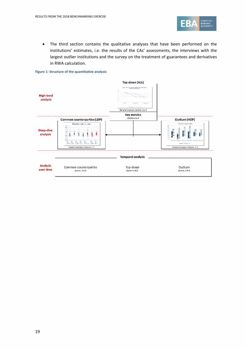
Figure 1: Structure of the quantitative analysis ....................................................................... 19
Figure 2: Share of exposures under LDPs, under HDPs and outside the scope of the 2018 SVB exercise (comparison with total IRB portfolio from COREP data) (sorted by the share under LDPs from largest to smallest) ........................................................................................................ 27
Figure 3: Portfolio composition of RWA (outer circle) and EAD (inner circle) for HDPs and LDPs (defaulted and non-defaulted) ............................................................................................... 28
Figure 4: Portfolio composition of the LDPs: share of large corporates, institutions and sovereigns in LDPs (sorted by the share of large corporates in LDPs from largest to smallest) ................... 29
Figure 5: Portfolio composition of the HDPs: share of residential mortgages, SME retail, SME corporate and corporate-other exposures in HDPs (sorted by the share of mortgages in HDPs from largest to smallest) ................................................................................................................ 30
Figure 6: Share of EAD (inner circle) and RWA (outer circle) for defaulted and non-defaulted exposures, LDPs and HDPs ..................................................................................................... 30
Figure 7: Share of EAD (inner circle) and RWA (outer circle) for defaulted and non-defaulted exposures by SVB portfolios (LDPs) ........................................................................................ 31
Figure 8: Share of EAD (inner circle) and RWA (outer circle) for defaulted and non-defaulted exposures by SVB portfolios (HDPs) ....................................................................................... 32
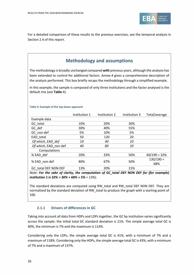
Figure 9: GC dispersion (delta Q3 – Q1), broken down by default status, for LDP and HDP exposures .............................................................................................................................. 36
Figure 10: Decomposition of the GC standard deviation index – HDPs and LDPs ...................... 37
Figure 11: Decomposition of the GC standard deviation index – LDPs ...................................... 38
Figure 12: Decomposition of the GC standard deviation index – HDPs ..................................... 38
Figure 13: GC and RW, for defaulted and non-defaulted exposures, by institution, LDPs (top panel) and HDPs (bottom panel) ....................................................................................................... 40
Figure 14: Adjusted GC and RW, for defaulted and non-defaulted exposures, by institution, LDPs (top panel) and HDPs (bottom panel) ..................................................................................... 41
Figure 15: LDP common counterparties compared with corresponding IRB EAD or RWA from COREP data ........................................................................................................................... 44
Figure 16: RW deviations for large corporate counterparties (AIRB and FIRB) .......................... 46
Figure 17: Dispersion of RW deviations, by regulatory approach – sovereigns ......................... 47
Figure 18: Dispersion of RW deviations, by regulatory approach – institutions ........................ 47
Figure 19: Interquartile range of the ratio of DR1Y to PD and the ratio of DR5Y to PD, for non-defaulted exposures, by SVB exposure class and regulatory approach..................................... 51
Figure 20: Range of the ratio of LR1Y to LGD and the ratio of LR5Y to LGD, for non-defaulted exposures, by portfolio and regulatory approach.................................................................... 52
Figure 21: Common EAD among the 2016, 2017 and 2018 SVB exercises (EUR millions) ........... 53

RESULTS FROM THE 2018 BENCHMARKING EXERCISE
4
Figure 22: Comparison of RWs, PD and LGD in current and previous SVB exercises (defaulted and non-defaulted exposures) ...................................................................................................... 54
Figure 23: Comparison of RWs by SVB exposure class in current and previous SVB exercises (defaulted and non-defaulted exposures) ............................................................................... 54
Figure 24: Comparison of PDs by SVB exposure class in current and previous SVB exercises (defaulted and non-defaulted exposures) ............................................................................... 55
Figure 25: Comparison of LGDs by SVB exposure class in current and previous SVB exercises (defaulted and non-defaulted exposures) ............................................................................... 55
Figure 26: Comparison of the top-down analysis for LDPs in the 2017 and 2018 exercises (common sample) ................................................................................................................................. 56
Figure 27: Comparison of the top-down analysis for HDPs in the 2016 and 2018 exercises (common sample) .................................................................................................................. 57
Figure 28: Share of EAD in the common subsample................................................................. 58
Figure 29: Evolution of the common subsample from the 2015 LDP exercise to the 2017 LDP exercise, by SVB exposure class .............................................................................................. 59
Figure 30: Evolution of RW, PD and LGD volatility ................................................................... 60
Figure 31: Default rate to PD ratio trend ................................................................................. 61
Figure 32: Loss rate to LGD ratio trend ................................................................................... 62
Figure 33: RWA** and RWA* versus RWA trend ..................................................................... 62
Figure 34: CA’s overall assessment of the level of institutions’ own funds requirements, taking into account benchmark deviations........................................................................................ 64
Figure 35: Positive and negative deviations justified (at least one parameter) ......................... 65
Figure 36: Common reasons for negative deviations not justified (at least one parameter) ...... 66
Figure 37: Has the institution’s internal validation of the model identified the most relevant possible unjustified negative deviations? ............................................................................... 69
Figure 38: Have the CA’s monitoring activities (ongoing or on-site) of the internal models identified the most relevant possible unjustified negative deviations? .................................... 70
Figure 39: Are any actions planned by the CA following the SVB results? ................................. 71
Figure 40: Institutions taking guarantees or derivatives into account for the purpose of RWA calculation ............................................................................................................................. 74
Figure 41: Distribution of methodologies for the treatment of guarantees and derivatives in RWA calculation by type of guarantor ............................................................................................ 75
Figure 42: Distribution of methodologies for the treatment of guarantees and derivatives in RWA calculation by type of guarantor (corporate non-SME exposures in the AIRB) .......................... 76
Figure 43: Distribution of methodologies for the treatment of guarantees and derivatives in RWA calculation by type of guarantor (corporate non-SME exposures in the FIRB) .......................... 76
Figure 44: Distribution of methodologies for the treatment of guarantees and derivatives in RWA calculation by type of guarantor (mortgages) ......................................................................... 77
Figure 45: How are PD adjustments performed? ..................................................................... 77

RESULTS FROM THE 2018 BENCHMARKING EXERCISE
5
Figure 46: How are LGD adjustments performed? ................................................................... 78
Figure 47: If using PD and/or LGD substitution, is the RW function changed? .......................... 79
Figure 48: Effect of the use of guarantees and/or derivatives on the PD estimate .................... 80
Figure 49: Effect of the use of guarantees and/or derivatives on the LGD estimate .................. 81
Figure 50: Effect of the use of guarantees and/or derivatives on the RW ................................. 81
Figure 51: RW dispersion (delta Q3 – Q1) of the different SVB exposure classes (defaulted and non-defaulted exposures) ...................................................................................................... 97
Figure 52: RW dispersion (delta Q3 – Q1) for the different SVB exposure classes and default status (HDPs and LDPs) .................................................................................................................... 98
Figure 53: Evolution of EAD by SVB portfolio and regulatory approach .................................... 99
Figure 54: Change in EAD by regulatory approach (EUR millions) ............................................105
Figure 55: Change in EAD-weighted RW by regulatory approach ............................................106
Figure 56: Change in EAD-weighted PD by regulatory approach .............................................107
Figure 57: Change in EAD-weighted LGD by regulatory approach ...........................................108
Figure 58: RW distribution for sovereign non-defaulted exposures, by country of residence of the portfolio ...............................................................................................................................110
Figure 59: RW distribution for corporate non-defaulted exposures, by country of residence of the portfolio ...............................................................................................................................110
Figure 60: RW distribution for non-defaulted exposures to institutions, by country of residence of the portfolio .....................................................................................................................110
Figure 61: RW distribution for large corporate non-defaulted exposures, by country of residence of the portfolio .....................................................................................................................111
Figure 62: RW distribution for residential mortgage non-defaulted exposures, by country of residence of the portfolio .....................................................................................................111
Figure 63: RW distribution for SMEC non-defaulted exposures, by country of residence of the portfolio ...............................................................................................................................111
Figure 64: RW distribution for SMER non-defaulted exposures, by country of residence of the portfolio ...............................................................................................................................112
Figure 65: Median, first and third quartile of the interquartile range (Q3 – Q1) of the RWs by country of the common counterparties for exposures to large corporates ..............................113
Figure 66: Median, first and third quartile of the interquartile range (Q3 – Q1) of the RWs by country of the common counterparties for exposures to institutions .....................................113
Figure 67: Comparison of the PD and the default rate (past year and past 5 years), for the SME retail portfolio, for non-defaulted exposures, for the AIRB approach, by country of residence of the counterparties (with at least five institutions) .................................................................114
Figure 68: Comparison of the LGD and the loss rate (past year and past 5 years), for the SME retail portfolio, for non-defaulted exposures, for the AIRB approach, by country of residence of the counterparties (with at least five institutions) .......................................................................115
RESULTS FROM THE 2018 BENCHMARKING EXERCISE
6
Figure 69: Comparison of the PD and the default rate (past year and past 5 years), for the SME corporate portfolio, for IRB (FIRB and AIRB) non-defaulted exposures, by country of residence of the counterparties (with at least five institutions) .................................................................116
Figure 70: Comparison of the LGD and the loss rate (past year and past 5 years), for the SME corporate portfolio, for IRB (FIRB and AIRB) non-defaulted exposures, by country of residence of the counterparties (with at least five institutions) .................................................................118
Figure 71: Comparison of the PD and the default rate (past year and past 5 years), for the corporate-other portfolio, for IRB (FIRB and AIRB) non-defaulted exposures, by country of residence of the counterparties (with at least five institutions) ..............................................119
Figure 72: Comparison of the LGD and the loss rate (past year and past 5 years), for the corporate-other portfolio, for IRB (FIRB and AIRB) non-defaulted exposures, by country of residence of the counterparties (with at least five institutions) .......................................................................120
Figure 73: Comparison of the PD and the default rate (past year and past 5 years), for the residential mortgages portfolio, for IRB AIRB non-defaulted exposures, by country of residence of the counterparties (with at least five institutions) .............................................................121
Figure 74: Comparison of the LGD and the loss rate (past year and past 5 years), for the residential mortgages portfolio, for IRB AIRB non-defaulted exposures, by country of residence of the counterparties (with at least five institutions) .......................................................................122

RESULTS FROM THE 2018 BENCHMARKING EXERCISE
7
List of tables
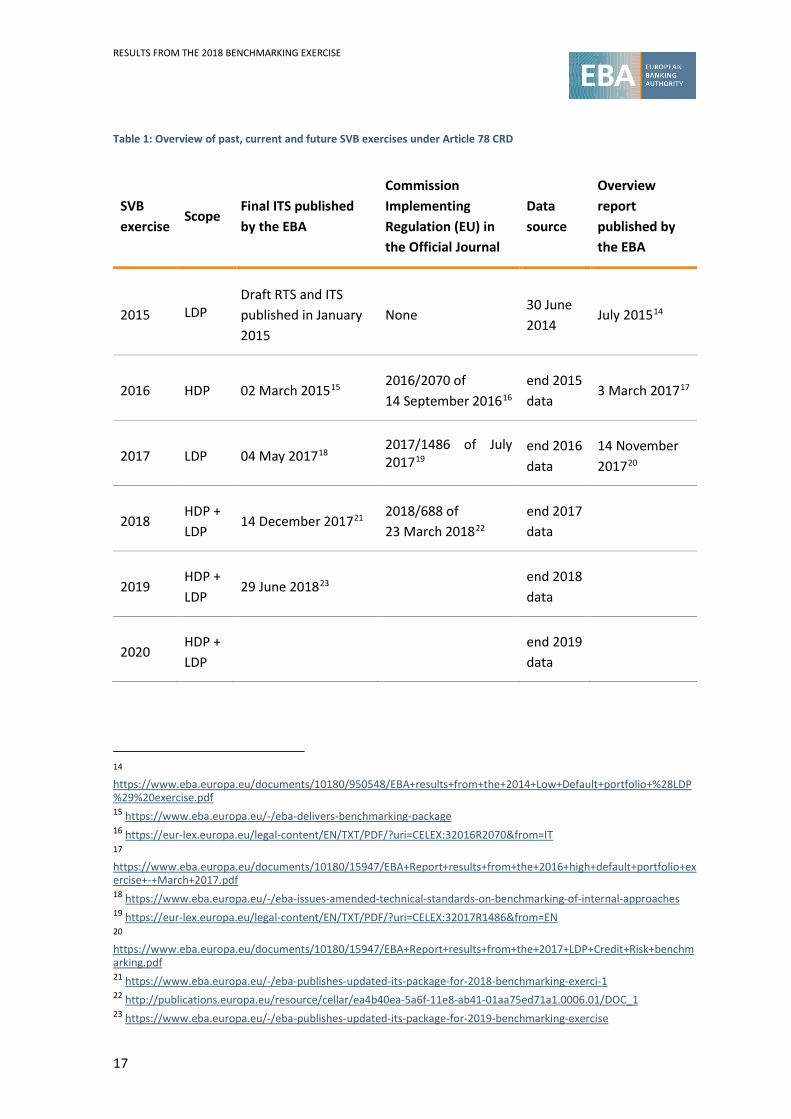
Table 1: Overview of past, current and future SVB exercises under Article 78 CRD ................... 17
Table 2: Use of different regulatory approaches by SVB exposure class ................................... 25
Table 3: Summary statistics on the share of exposures under LDPs, under HDPs and outside the scope of the SVB exercise ...................................................................................................... 27
Table 4: Example of the top-down approach .......................................................................... 35
Table 5: Summary statistics of the key metrics observed for non-defaulted exposures, by SVB exposure class and regulatory approach ................................................................................. 42
Table 6: Summary statistics on the RW deviations (1st and 3rd quartile, median and interquartile range) by SVB exposure class and regulatory approach ........................................................... 45
Table 7: Key metrics at portfolio level .................................................................................... 50
Table 8: Summary statistics of the ratio of the DR1Y to PD and the ratio of the DR5Y to PD, for non-defaulted exposures, by SVB exposure class and regulatory approach.............................. 50
Table 9: Interquartile range of the ratio of LR1Y to LGD and the ratio of LR5Y to LGD, for non-defaulted exposures, by SVB exposure class and regulatory approach..................................... 51
Table 10: Number of observations (institutions), by SVB exposure class, reporting yes or no, on whether they use guarantees and/or derivatives in RWA calculations ..................................... 80
Table 11: List of institutions participating in this exercise ........................................................ 87
Table 12: Sample of institutions, countries and counterparties in the common counterparty analysis (LDPs) ....................................................................................................................... 93
Table 13: Sample of institutions, countries and counterparties in the portfolio analysis (LDPs) (C 102.00) .............................................................................................................................. 94
Table 14: Sample of institutions, countries and counterparties in the portfolio analysis (HDPs) (C 103.00) .............................................................................................................................. 94
Table 15: Number of counterparties in the common counterparty analysis, by regulatory approach ............................................................................................................................... 99

RESULTS FROM THE 2018 BENCHMARKING EXERCISE
8
Abbreviations
AIRB advanced internal ratings-based
CA competent authority
CCF credit conversion factor
CGCB central governments and central banks
COREP common supervisory reporting
CORP exposures to corporates other
CRD Capital Requirements Directive
CRM credit risk mitigation
CRR Capital Requirements Regulation
DR default rate
DR1Y 1-year default rate
DR5Y 5-year default rate
EAD exposure at default
EBA European Banking Authority
EL expected loss
ELBE best estimate of expected loss
EU European Union
FIRB foundation internal ratings-based
GC global charge
GG sovereign exposure
HDP high default portfolio
IMI internal model inspection

RESULTS FROM THE 2018 BENCHMARKING EXERCISE
9
INST exposures to institutions
IRB internal ratings-based
ITS implementing technical standards
LC large corporate
LCORP exposures to large corporates
LDP low default portfolio
LEI Legal Entity Identifier
LGD loss given default
LR loss rate
LR1Y 1-year loss rate
LR5Y 5-year loss rate
LTV loan-to-value
M maturity
MoC margin of conservatism
MORT exposures to residential mortgages
PD probability of default
PIT point in time
PPU permanent partial use
RW risk weight
RWA risk-weighted asset
SA standardised approach
SLSC specialised lending slotting criteria
SMEs small and medium-sized enterprises
SMEC exposures to corporate SMEs
RESULTS FROM THE 2018 BENCHMARKING EXERCISE
10
SMER exposures to retail SMEs
STD standard deviation
SVB supervisory benchmarking
TRIM targeted review of internal models
TTC through the cycle
UFCP unfunded credit protection
UL unexpected loss

RESULTS FROM THE 2018 BENCHMARKING EXERCISE
11
Executive summary
This report presents the results of the 2018 supervisory benchmarking (SVB) exercise for both high default portfolios (HDPs) and low default portfolios (LDPs). For the LDPs, the following SVB exposure classes1 are considered: exposures to large corporates, sovereigns and institutions. For the HDPs, the following SVB exposure classes are considered: residential mortgages, small and medium-sized enterprise (SME) retail, SME corporate and corporate-other portfolios. The aim of this study is to not only assess the overall level of variability in risk-weighted assets (RWAs) but also examine and highlight the different drivers of the dispersion observed. In addition, this report provides a broad overview to the public on how the data collected through the implementing technical standards (ITS) on SVB have been used for the purpose of identifying outlier institutions.
The analysis is based on data reported at the highest level of consolidation, ensuring that the same data are used only once in the calculation of the benchmarks. The reference date for the data used in this report is 31 December 2017; 117 institutions had their credit risk internal models approved on that date, of which 114 across 17 European Union (EU) countries contributed to this exercise, submitting at least one counterparty and/or portfolio (this is because three institutions do not have exposures within the scope of the SVB exercise, because of their specialised business models). Qualitative information on specific aspects has been collected through (i) individual assessments by competent authorities (CAs) of all institutions, (ii) interviews with a sample of 11 institutions and (iii) a qualitative survey distributed to all institutions.
Building on the previous reports, three main analyses have been performed this year to examine drivers of risk weight (RW) variability: a top-down study (for both HDPs and LDPs), a common counterparties analysis (only for LDPs) and an outturn analysis (only for HDPs). These analyses have been complemented by assessments by the CAs of each of the institutions, interviews with the 11 institutions for which the highest numbers of outlier observations2 were reported, an ad hoc survey on the use of the substitution effect and a comparison of the main indicators over time.
Given the limitations of and assumptions underlying the different approaches, their findings should be considered as a whole. In addition, some data quality issues3, which are identified throughout the report, suggest that the results of the analyses should be interpreted with caution.
Main findings from the top-down approach
1 SVB exposure classes are different from exposure classes as referred to in the CRR in Article 147(2). SVB exposure classes are large corporates, sovereigns, institutions, residential mortgages, SME retail, SME corporate and corporate-other exposures. 2 An outlier observation indicates that an observation has been marked when it is below a certain threshold. It does not indicate, per se, that the risk weights are underestimated, but instead triggers a further review. 3 See also Annex 2.

RESULTS FROM THE 2018 BENCHMARKING EXERCISE
12
Beginning by considering the concept of global charge (GC) variability4, based on the standard deviation across institutions, the European Banking Authority (EBA) took a top-down approach to quantifying the proportion of variability that can be explained by some key drivers. Differences in (i) the share of the defaulted exposures and (ii) the portfolio mix effect explain around 50% of GC variability observed in the data. The remaining 50% may be due to differences in collateralisation and other institution-specific factors, such as risk strategy and management practices, portfolio composition and client structure. This confirms previous findings that RWA variability can be explained, to a large extent, by looking at some measurable features of institutions’ exposures.
Main findings from the common counterparties analysis
For each institution and each of its obligors belonging to the predefined list of counterparties, the deviation from the benchmark value has been computed, based on median probability of default (PD), loss given default (LGD) and maturity (M) parameters. The results show that most of the interquartile ranges of the RW deviations resulting from benchmark substitutions are below 10%. These interquartile differences are greater under the advanced internal ratings-based (AIRB) approach than under the foundation internal ratings-based (FIRB) approach for large corporates and sovereigns. In the AIRB approach, these interquartile differences are greatest for exposures to large corporates, and this stems from the variability introduced by the PD and the unsecured LGD. Variability in the maturity parameter is the greatest contributor to the RW dispersion for sovereign exposures.
Finally, there is a strong non-linearity effect, in the sense that the variability of the different risk parameters has a compensating effect (the total deviation is well below the sum of the deviation of each risk parameter): in short, low PD estimates are generally associated with high LGD estimates, and vice versa.
Main findings from the outturn (‘backtesting’) approach
The outturn (‘backtesting’) approach compares observed values (default rates (DRs) and loss rates (LRs)) (for the past year and for the past 5 years on average) with estimated values (PDs and LGDs) for the individual institutions, for the different portfolios and regulatory approaches. In addition, the hypothetical RWA, computed on the basis of a comparison of the institution’s PD with its adjusted default rate, is compared with the RWA as reported by the institution.
The results show that this hypothetical RWA is equal to the reported RWA for at least half of the institutions. Overall, the analysis does not reveal a material negative deviation of the estimated level of risk compared with the observed level of risk for the vast majority of EU institutions.
4 In this report, the analysis is based on two main indicators: the EAD-weighted average RW, or so-called RWA density, and the weighted average GC, which is calculated for IRB exposures as (12.5 × EL + RWA) ÷ EAD. To analyse the variability, the standard deviation of the indicators observed at institution level is computed. Complementary metrics to the variability considered in this study are the interquartile range and the maximum versus minimum distance.

RESULTS FROM THE 2018 BENCHMARKING EXERCISE
13
With regard to the ratio of the default rate to the PD estimate, the results show that the great majority of institutions have conservative estimates, in particular when compared with the observed values for the past year. This analysis corroborates that the portfolio mix and the regulatory approach are key determinants in explaining variability. The additional country analysis suggests that this is also a driver of variability.
With regard to the ratio of the loss rate and the LGD estimate, the results show that for at least 75% of institutions the portfolio estimated LGD is higher than the loss rate observed either in the past year or over the past 5 years, which could again indicate conservative behaviour on the part of the institutions5.
Analysis of variability over time
This year’s SVB exercise is based on data from both the HDPs and LDPs, and these data can be compared with the 2016 HDP exercise and the 2017 LDP exercise. This makes a comparison of the variability found in this exercise and in the previous ones possible. For this purpose, a sample of common institutions was created, i.e. institutions that participated in the 2016 HDP exercise, the 2017 LDP exercise and this year’s exercise. The results show that, whereas there has been a slight increase in the exposures covered, there is stability in the reported parameters, such as RW, PD and LGD, with the exception of the PD for large corporates under the FIRB, for which an increase was observed.
For the LDPs, a comparison of the variability (in terms of RW, PD and LGD) of the common counterparties by SVB exposure class has been performed. It can be noted that the variability in estimates is very stable over the two exercises.
For the HDPs, the results of this year’s SVB exercise compared with those of the 2016 exercise show that, in general, both default and loss rates have been decreasing more than PD and LGD estimates in recent years. This is likely to reflect a general improvement in economic conditions.
Main findings from CAs’ assessments based on supervisory benchmarks
CAs provided individual assessments of the quality of the benchmarked models for each institution based on the outcomes of the SVB exercise. For the majority of the institutions, the RW deviations from the EU benchmarks were deemed by the CAs to be justified. The highest share of unjustified negative deviations from the benchmark were observed for exposures to corporates (corporate SME exposures, corporate-other exposures and large corporate exposures), for which such
5 However, since the loss rate in the analysis is not purely observed, but calculated using the institution’s estimate, these results should be interpreted with caution and complemented by a case-by-case analysis. In addition, this could be a reflection of the fact that LGD estimates should be appropriate for an economic downturn (see Article 181(1)(b) of the Capital Requirements Regulation (CRR)).

RESULTS FROM THE 2018 BENCHMARKING EXERCISE
14
deviations have been flagged in the case of around 15% of institutions. It should, however, be kept in mind that these are outlier values resulting from modelling, which are treated as an indication of potentially significant differences in own funds requirements, and which therefore need a specific assessment by the CA.
Problems with the calibration of the risk parameters are mentioned as the main reason for the unjustified underestimations, but there are other concerns related to, inter alia, data quality, differences in definitions used, the design of the ranking model, the absence of models for LGD-in-default estimates and best estimate of expected loss (ELBE), and deficiencies in the framework for the review of estimates. It is reassuring that most practice-based aspects are being addressed in the EBA GLs on PD and LGD estimation6.
The CAs’ assessments also revealed that the majority of institutions’ internal validations identified the unjustified negative deviation identified in the SVB exercise. In those cases where unjustified negative deviations were identified but the internal validation unit was not aware of any issue, the main reason mentioned was that the institution’s model validation function was not yet fully developed and needed to be reinforced, or that proper guidelines were lacking. It is also reassuring that the CAs’ monitoring activities (ongoing or on-site) had identified most of the issues related to the unjustified negative deviations detected by the SVB exercise. For a small sample of institutions, the unjustified negative deviations identified by the SVB exercise will lead to further action by the CA. This proves the usefulness of the SVB exercise in identifying undue RWA variability as a driver of model improvement. For the other unjustified negative deviations, the CA was already aware of the issue, and an internal model inspection (IMI) is either planned or is currently taking place, or the institution is currently redeveloping and/or recalibrating its model, or a (material) model change has already taken place.
In comparison with previous exercises (the 2016 HDP exercise and the 2017 LDP exercise), institutions’ internal validations as well as the CAs’ monitoring activities (ongoing or on-site) are increasingly picking up on issues identified by the EBA SVB exercise. This is reassuring and indicates that the increased regulatory and supervisory attention paid to internal models is contributing to the consistency of the RWA of internal models.
Main findings from the interviews
The EBA has, together with the CAs, conducted interviews with the 11 institutions for which the highest number of outlier observations were spotted. In general, the interviews were useful because they allowed a number of points to be clarified.
For LDPs, many of the identified outlier observations relate to methodological problems with techniques to overcome data scarcity, i.e. extrapolation techniques, problems with backtesting, or difficulties with calibration techniques at a portfolio level.
6 https://www.eba.europa.eu/documents/10180/2033363/Guidelines+on+PD+and+LGD+estimation+%28EBA-GL-2017-16%29.pdf/6b062012-45d6-4655-af04-801d26493ed0

RESULTS FROM THE 2018 BENCHMARKING EXERCISE
15
For HDPs, the interviews highlighted that, in some cases, the institution had performed its risk quantification at the grade or pool level without checking homogeneity at the grade level. In other cases, there was no treatment of incomplete workout scenarios. Finally, some of the outlier observations were due to sensitivity to the definitions used for the SVB exercise (exposure-weighted versus obligor-weighted parameters).
One recurring topic arising from the interviews was the quality of data, i.e. several of the issues identified could be explained by data quality problems. Furthermore, there seemed to be several misunderstandings with respect to the revised concept of margin of conservatism (MoC), as introduced in the EBA Guidelines on PD and LGD.
Main findings from the survey on substitution effect The EBA launched a survey to gain an overview of the current practices on how guarantees and derivatives are taken into account for the purpose of RWA calculation and, in particular, whether SVB parameters are biased as a result of the incorporation of guarantees and/or derivatives into RW calculation. The results show that the majority of institutions take guarantees or derivatives into account for the purpose of RWA calculation in the exposure classes covered in the survey (corporate non-SME under the FIRB and AIRB approaches and mortgages). However, the materiality of guarantees and/or derivatives in RWA calculation seems to be limited, in the sense that the share of the portfolios that are covered is usually in the range of 1% to 5%, with only a few exceptions of up to 10%.
Standardised approach (SA) guarantors are taken into account mostly via RW substitution, whereas FIRB guarantors are taken into account mostly via PD substitution. AIRB guarantors are taken into account via a range of different methods. Based on the results from the survey, it is not possible to find evidence that the use of guarantees and/or derivatives significantly affects the level of PD, LGD and/or RW estimates. Nevertheless, it is still possible that outlier detection is adversely affected by the use of guarantees and/or derivatives.

RESULTS FROM THE 2018 BENCHMARKING EXERCISE
16
Introduction and legal background
This report presents the results of the SVB exercise on the internal models used for both HDPs7 and LDPs8 across a sample of EU institutions. The reference date for the data is 31 December 2017. The underlying framework was designed by the EBA via the final draft ITS published by the EBA in December 2017 9 and published as Commission Implementing Regulation (EU) 2018/688 of 23 March 201810. It is the first time that the results of the HDPs and LDPs have been presented in a joint report. However, previous studies have been published on the topic11:
• on the HDPs, published by the EBA in December 201312 and June 201413;
• on the LDPs, published by the EBA in February 2013 and August 2013.
Since 2015, these studies have formed part of yearly SVB exercises that are prescribed by Article 78 of the Capital Requirements Directive (CRD), which sets out requirements for institutions, CAs and the EBA concerning the establishment of a regular SVB process to assess the internal models used to compute own funds requirements (with the exception of operational risk). Table 1 provides an overview of the past, current and future SVB exercises and how they link to EBA ITS, Commission Implementing Regulations and EBA reports.
7 HDPs include residential mortgage, SME retail, SME corporate and corporate-other portfolios. 8 LDPs consist of sovereigns, institutions and large corporates, as these portfolios generally contain few defaults relative to the total number of obligors. Previous studies on the topic of LDPs were published in 2015 and 2017. 9 https://www.eba.europa.eu/-/eba-publishes-updated-its-package-for-2018-benchmarking-exerci-1 10 http://publications.europa.eu/resource/cellar/ea4b40ea-5a6f-11e8-ab41-01aa75ed71a1.0006.01/DOC_1 11 All reports on RWA consistency are available on the EBA website (http://www.eba.europa.eu/risk-analysis-and-data/review-of-consistency-of-risk-weighted-assets/-/topic-documents/Dj0TmcAgAa0J/more). 12 EBA Third interim report on the consistency of risk-weighted assets: SME and residential mortgages. https://www.eba.europa.eu/documents/10180/15947/20131217+Third+interim+report+on+the+consistency+of+risk-weighted+assets+-+SME+and+residential+mortgages.pdf 13 EBA Fourth report on the consistency of risk-weighted assets: Residential mortgages drill-down analysis. http://www.eba.europa.eu/documents/10180/15947/20140611+Fourth+interim+report+on+the+consistency+of+risk-weighted+asset.pdf
RESULTS FROM THE 2018 BENCHMARKING EXERCISE
17
Table 1: Overview of past, current and future SVB exercises under Article 78 CRD
SVB exercise
Scope Final ITS published by the EBA
Commission Implementing Regulation (EU) in the Official Journal
Data source
Overview report published by the EBA
2015 LDP Draft RTS and ITS published in January 2015
None 30 June 2014
July 201514
2016 HDP 02 March 201515 2016/2070 of 14 September 201616
end 2015 data
3 March 201717
2017 LDP 04 May 201718 2017/1486 of July 201719
end 2016 data
14 November 201720
2018 HDP + LDP
14 December 201721 2018/688 of 23 March 201822
end 2017 data
2019 HDP + LDP
29 June 201823 end 2018 data
2020 HDP + LDP
end 2019 data
14 https://www.eba.europa.eu/documents/10180/950548/EBA+results+from+the+2014+Low+Default+portfolio+%28LDP%29%20exercise.pdf 15 https://www.eba.europa.eu/-/eba-delivers-benchmarking-package 16 https://eur-lex.europa.eu/legal-content/EN/TXT/PDF/?uri=CELEX:32016R2070&from=IT 17 https://www.eba.europa.eu/documents/10180/15947/EBA+Report+results+from+the+2016+high+default+portfolio+exercise+-+March+2017.pdf 18 https://www.eba.europa.eu/-/eba-issues-amended-technical-standards-on-benchmarking-of-internal-approaches 19 https://eur-lex.europa.eu/legal-content/EN/TXT/PDF/?uri=CELEX:32017R1486&from=EN 20 https://www.eba.europa.eu/documents/10180/15947/EBA+Report+results+from+the+2017+LDP+Credit+Risk+benchmarking.pdf 21 https://www.eba.europa.eu/-/eba-publishes-updated-its-package-for-2018-benchmarking-exerci-1 22 http://publications.europa.eu/resource/cellar/ea4b40ea-5a6f-11e8-ab41-01aa75ed71a1.0006.01/DOC_1 23 https://www.eba.europa.eu/-/eba-publishes-updated-its-package-for-2019-benchmarking-exercise

RESULTS FROM THE 2018 BENCHMARKING EXERCISE
18
The main objectives of this report can be summarised as (i) providing an overview of the existing RWA variability and drivers of differences for the reference date (31 December 2017); (ii) summarising the latest results of the supervisory assessments of the quality of the internal approaches in use; and (iii) providing evidence to policymakers for future activities relating to RWA differences.
The data collection is based on technical standards specifically designed for annual SVB exercises and covers different breakdowns of portfolios by, for instance, country, type of collateral, loan-to-value (LTV) ratio or sector, to help us understand the impact of these factors on the different key risk drivers such as PD, LGD, credit conversion factor (CCF) and RW estimates. In addition, some qualitative information and more in-depth information on specific aspects – such as institutions’ modelling methodologies, data sources, lengths of time series, definitions of risk parameters and number and scope of internal models – have been collected through interviews and a qualitative survey.
These studies form part of yearly SVB exercises, requiring institutions, CAs and the EBA to set up regular SVB processes to assess the internal models used to compute own funds requirements (with the exception of operational risk):
• In accordance with Article 78 of the CRD, CAs need to, at least annually, make an assessment of the quality of the institutions’ internal approaches. Each CA shares the outcome of its assessment with the EBA and the other relevant CAs (home and host CAs). The regular supervisory benchmarks on internal approaches developed by the EBA and shared with the CAs are considered a useful supervisory monitoring tool to support the CAs’ assessments of internal models.
• The EBA provides feedback to institutions that participated in the exercise on benchmark parameters at portfolio level in order to complement the information available to institutions for monitoring their internal models. The EBA considers that feedback on benchmark parameters provides positive incentives for institutions to continuously improve the quality of their regular data submissions for future SVB exercises.
The report is organised as follows:
• The first section gives a general description of the exercise and provides the main statistics on the data collected.
• The second section contains a quantitative analysis of the variability of the collected data (see Figure 1 for an overview of the different analyses). The first three subsections replicate the three analyses conducted in the previous reports. Starting from a high-level analysis taking a top-down approach to the whole portfolio, the report presents key distribution statistics, before moving to a deeper analysis (the common counterparties analysis for LDPs and the outturn analysis for HDPs). The last subsection replicates the three analyses with a time perspective (a comparison of the results with the results of the previous reports).
RESULTS FROM THE 2018 BENCHMARKING EXERCISE
19
• The third section contains the qualitative analyses that have been performed on the institutions’ estimates, i.e. the results of the CAs’ assessments, the interviews with the largest outlier institutions and the survey on the treatment of guarantees and derivatives in RWA calculation.
Figure 1: Structure of the quantitative analysis

RESULTS FROM THE 2018 BENCHMARKING EXERCISE
20
1. Section 1: General description
1.1 Dataset and assessment methodology
1.1.1 Dataset
Altogether, 117 institutions24 from 17 EU countries have approval for the use of credit risk internal models at 31 December 2017 and are therefore in the scope of the 2018 SVB exercise. In comparison with previous studies, the number of institutions in the sample is stable. The figures presented in this report are at the highest level of consolidation. Although 117 institutions have the authorisation for the credit risk internal models, only 114 institutions submitted data for at least one counterparty or one portfolio (this is because three institutions do not have exposures within the scope of the SVB exercise, because of their specialised business models, so they submitted empty templates) (of which 112 submitted at least one valid record). The reference date for the data of this report is 31 December 2017.
The report relies on data collected in accordance with the ITS on SVB25 (complemented by common supervisory reporting (COREP)26 data when necessary) through six different templates:
• Template C 101.0027 provides the information at counterparty level (‘common sample’) for a given list of counterparties. The common sample of counterparties was defined by the EBA, and institutions were requested to provide the PDs and LGDs, as well as the hypothetical senior unsecured LGDs, for those counterparties included in the ‘common portfolio’ on which they had an exposure or a valid rating at the reference date28.
24 At the EU level, 124 institutions have approval for use of an internal model, of which 117 institutions have approval for the use of credit risk models. Of the 117 institutions (versus 118 of previous year) that have approval for the use of credit risk internal models and that participated in this exercise, across 17 EU countries. 114 of them submitted at least 1 counterparty and/or one portfolio. 25 Annex I of the ITS provides the definitions of the SVB portfolios that are required for the 2018 exercise. Annex III of the ITS provides the instructions and details on exposures, that is, the data collected. In addition, Annex III also provides further details of internal models and the mapping of internal models (Templates C 105.1 and C 105.2, respectively; see Annexes) to portfolios (Annexes II and IV of the ITS). 26 COREP requirements are specified by the EBA via the ITS, which was adopted by the Commission as Regulation 680/2014. 27 In total, 85 institutions submitted the template with at least one counterparty with the EAD greater than zero. 28 Since the end of 2017, some of the models under review have been updated/replaced, so the analysis is a point-in-time assessment, and some of the findings have since been mitigated. Only records with an exposure greater than zero were used for the analysis.

RESULTS FROM THE 2018 BENCHMARKING EXERCISE
21
• Template C 102.00 29 provides the information on various LDPs (large corporates 30 , institutions and sovereigns). These data are used for the top-down analysis and include information on the institution’s actual exposure values and IRB parameters. Similarly to previous exercise, there is no information on SA exposures (either on a roll-out plan or under the permanent partial use (PPU) allowance), or on portfolios other than the LDPs.
• Template C 103.0031 provides the same kind of information as template C 102.00 with the addition of some backtesting parameters but for the HDPs (corporates other, SME retail, SME corporates and residential mortgages)32.
• Templates C 105.01, C 105.02 and C 105.03 contain details on the internal models and give the link between the EBA supervisory benchmark portfolios and the models concerned.
For risk parameters such as PDs and LGDs, the results of the exercise are based on the parameters used for the calculation of the institutions’ own funds requirements, i.e. the comparison of institutions does not take into account whether or not supervisory corrective actions aimed at increasing RWs to correct any model deficiencies (e.g. add-ons) have been imposed by some CAs on institutions’ models.
1.1.2 Challenges encountered when analysing the variability of IRB models’ outcomes
The most challenging part in comparative RWA studies is to distinguish the influence of risk-based and practice-based drivers. As shown in this report, the ‘top-down’ analysis can explain a substantial percentage of the variability observed in some key drivers. However, the remaining variability needs to be approached differently. Specific challenges arise depending on the type of analysis applied:
• LDPs generally show so few data, and in particular defaults, that historical data may not provide statistically significant differentiation between different portfolio credit risks 33. Instead, for these LDPs, IRB parameters and RWs can be compared for identical obligors to whom the institutions have real exposures. The key limitation of this approach is the
29 In total, 97 institutions submitted at least one of the portfolios listed in Annex I, template C 102.00. Of these, 91 reported at least one large corporate portfolio (of which 59 reported at least one portfolio under AIRB, 49 at least one portfolio under FIRB and 12 at least one portfolio under specialised lending slotting criteria (SLSC)); 68 reported at least one institutions portfolio (of which 38 were under AIRB and 44 under FIRB); and 51 reported at least one sovereign portfolio (of which 29 were under AIRB and 31 under FIRB). Some institutions reported portfolios under more than one regulatory approach for the same exposure class. 30 For the LDP exercises, large corporates are defined as firms with annual sales exceeding EUR 200 million. 31 In total, 108 institutions submitted at least one portfolio listed in Annex I, template C 103.00. 89 reported at least one Corporate other portfolio (of which: 55 at least one portfolio under AIRB, 51 reported at least one portfolio under FIRB and 19 at least one portfolio under SLSC), at least one portfolio for the Mortgages (under AIRB) and at least one for the SMER (of which: 55 at least one portfolio under AIRB, 49 at least one portfolio under FIRB, and 20 at least one portfolio under SLSC); 74 institutions reported at least one SMEC portfolio (under AIRB). 32 It does not include the remaining HDPs portfolios for instance credit card portfolios or consumer credits. 33 Owing to low PD estimates in LDPs for non-defaulted exposures, the influence of every default on the GC could be relatively large.

RESULTS FROM THE 2018 BENCHMARKING EXERCISE
22
representativeness of the common sample compared with the actual portfolio of each institution.
• On the other hand, and in contrast to the exercise for LDPs, for HDPs it is not possible to compare the same counterparties across institutions, but the large amount of available data and defaults in general allow a kind of statistical backtesting approach that represents an important source of information on the portfolio risk (outturns approach). This approach is very useful as the misalignment between estimates and observed parameters could suggest that differences in RWAs across institutions might be driven by differences in estimation practices (e.g. different levels of conservatism, adjustments to reflect long-run averages, different lengths of time series of the data available and included in the calibration of the cycle, assumptions underlying recovery estimates, etc.) and not only by differences in portfolio risk.
• Furthermore, a breakdown by country seems useful, since the risk profile of retail exposures is country-driven to some extent, so the comparisons across countries are more difficult to signal outliers. This is an important limitation and the reason why the outturn (backtesting) approach is a good and valuable process for comparing institutions, despite this approach also having some shortcomings. Observed parameters reported by institutions are largely influenced by the characteristics of the country, such as the macro-economic cycle, accounting framework and judicial system. Realised losses on defaulted exposures are influenced by the wide variation in loss recognition practices across jurisdictions, which influence the timing and the amounts of recorded losses, as well as by the limitations in the data used for estimations. However, the breakdown by country (in this report, the country of counterparty) can lead to data shortage and non-statistically relevant results.
In addition, different possible regulatory or supervisory requirements, such as regulatory floors34, could explain a substantial amount of differences by jurisdiction. In this context, it should be noted that the EBA has produced different regulatory products in order to harmonise the concepts and requirements of the IRB approach. This includes an RTS on the assessment methodology35, an RTS and guidelines on the definition of default36 and guidelines on the estimations of risk parameters37. In the same spirit, the 2018 data collection does not differentiate in the CORP and SMEC portfolios between specialised lending exposures that are not subject to the slotting approach and other non-
34 e.g. from Article 164(4) of the CRR: LGD floors for residential property are 10% and LGD floors for commercial property are 15%, and Article 164(5) of the CRR allows CAs to increase these regulatory floors. 35 https://www.eba.europa.eu/documents/10180/1525916/Final+Draft+RTS+on+Assessment+Methodology+for+IRB.pdf/e8373cbc-cc4b-4dd9-83b5-93c9657a39f0 36 RTS: https://eur-lex.europa.eu/legal-content/EN/TXT/?uri=CELEX:32018R0171 GL: https://www.eba.europa.eu/regulation-and-policy/credit-risk/guidelines-on-the-application-of-the-definition-of-default 37 GL: https://www.eba.europa.eu/regulation-and-policy/model-validation/guidelines-on-pd-lgd-estimation-and-treatment-of-defaulted-assets
RESULTS FROM THE 2018 BENCHMARKING EXERCISE
23
specialised lending exposures 38 . This can be problematic when trying to measure variability, because these exposures are significantly different in their nature and their embedded level of risk.
Finally, data quality is improving, but still remains problematic. The data collection for this exercise was based on a larger scope than in previous exercises, with data collected on both LDPs and HDPs. Institutions had different interpretations of some of the data fields, and these (while not strictly data errors) could explain some of the outlier values. The main data quality issues are listed in Annex 2. These data quality issues suggest that the results of the analysis should be interpreted with caution.
1.1.3 Analyses performed
The data were used to perform three main types of analyses in this report:
• Top-down and distribution analyses of institutions’ actual portfolios (for both LDPs and HDPs). These analyses mainly use the information collected via templates C 102 and C 103. Applying this method disentangles the impact of some key determinants of the GC on variability. The top-down analysis is complemented by a distribution analysis, which allows the identification of extreme values and values below the first quartile or above the third quartile for important parameters of the sample. The main advantage is that the distribution analysis allows outliers to be easily identified, after controlling for some portfolio characteristics. Further, the distribution analyses can be performed at different levels of aggregation and for different risk parameters. For instance, a comparison between regulatory approaches (e.g. FIRB and AIRB) at the EU level or at EU-country level for a particular portfolio (e.g. SME retail for non-defaulted exposures, in the construction sector) may allow possible drivers to be highlighted if there are significant differences between the approaches.
• Analysis of IRB parameters for common counterparties (for LDPs). This allows a PD and LGD comparison on an individual obligor basis. However, the subset of common obligors is, in most cases, not fully representative of the total IRB portfolio of the individual institutions, therefore the results of this exercise may not be transferable to the total IRB portfolios and should be interpreted with care.
• Outturns (backtesting) approach (for HDPs). This involves a comparison of observed values with estimated values for important parameters. It allows observed and estimated values to be compared and provides information about institutions’ realised credit performance history (default rates, loss rates and actual defaulted exposures, as well as averages of the past 5 years for default and loss rates) and the corresponding IRB parameters (PD, LGD and
38 It should be pointed out that this aspect has been rectified in the ITS for 2019 exercise.

RESULTS FROM THE 2018 BENCHMARKING EXERCISE
24
RWA), as well as PD backtesting results (RWA* and RWA**)39,40. These comparisons allow an analysis to be conducted on possible misalignments between estimated and observed parameters for the same institution.
Based on the data collected, an analysis is performed in order to identify the relevant outlier institutions that deserve further investigation by the CA. In a first step, several outlier observations are generated individually depending on the available data (LDPs, HDPs or all). For both HDPs and LDPs, the portfolios for which at least 10 institutions reported exposures have been used to assess potential outliers. The values of PD, LGD, CCF and the RW are assessed in terms of outliers and a flag is generated for each metric below the 10th percentile. For LDPs, another outlier rule is based on the common counterparties for which at least 10 institutions reported a rated exposure. The rule takes into account the PD, LGD, hypothetical unsecured LGD, CCF and the RW, and flags are generated for the 10 per cent lowest metrics reported. For HDPs, another outlier rule assesses the ratios of DR1Y/PD, DR5Y/PD, LR1Y/LGD and LR5Y/LGD, if the ratio can be computed for at least 10 institutions. Outlier observations are generated for the ratios higher than the 90th percentile. In a second step, an assessment is made between the number of outlier observations and the potential outlier observations to determine the final list of institutions and portfolios that deserve an in-depth investigation by the CAs.
Although these quantitative analyses are essential in such kind of exercise, the assumptions and caveats behind them make it clear that they should be complemented by a qualitative evaluation. Three different assessments have been performed:
• A qualitative survey on specific aspects of the credit risk mitigation (CRM) framework has been launched this year. Contrary to the other analyses in the report, the purpose of this survey is not to achieve a comprehensive view but rather to get a detailed view of the practices on one specific topic to help the policymaker in making choices. The focus of this year’s survey was decided in the light of the latest developments with regard to the EBA roadmap on the IRB models.
• CAs’ assessments of individual institutions in their jurisdictions have been shared with the EBA. Indeed, CAs are requested to share the evidence they have gathered among colleges of supervisors, as appropriate, and to take appropriate corrective actions to overcome
39 The risk-weighted exposure amounts, after applying the SME supporting factor, that would result from the application of PD* (derived from the case-weighted default rate for the last year for the rating grade) and PD** (derived from the case-weighted default rate for the past 5 years for the rating grade and the PD) instead of the original PD on the rating grade level shall be reported.
40 RWA*, which is the hypothetical RWA that results from the application of the maximum of PD and p*. For each counterparty grade, p∗ is the smallest positive value satisfying the equation:
p∗ + Φ−1(q) ∙ �p∗ ∙ (1 − p∗)
n ≥ DR1y
and RWA**, which is similar to RWA*, but using the DR5y instead of DR1y.
RESULTS FROM THE 2018 BENCHMARKING EXERCISE
25
drawbacks when deemed necessary. Using additional institution- and model-specific information from regular ongoing supervisory functions and EBA-computed benchmarks on risk parameters at counterparty and portfolio level has helped to identify potential non-risk-based variability across institutions. The SVB exercise allows CAs to assess the outcomes of institutions’ internal models compared with a wider scope of institutions.
• Finally, the EBA conducted interviews with 11 institutions to gather additional information. The selection of institutions for the interviews was based on the computed benchmarks on risk parameters and portfolios, with a special focus on conspicuous results. The aim of the interviews was to better understand the approaches taken by individual institutions to calculate own funds requirements and to identify key factors and drivers that can explain observed differences.
1.2 Portfolio composition and characteristics of institutions in the sample
This section describes the composition of the SVB sample in terms of a number of dimensions (i.e. the use of regulatory approaches across SVB exposure classes, the distribution of exposures across SVB exposure classes as well as in terms of defaulted versus non-defaulted exposures, and the representativeness of the sample).
1.2.1 Use of regulatory approaches
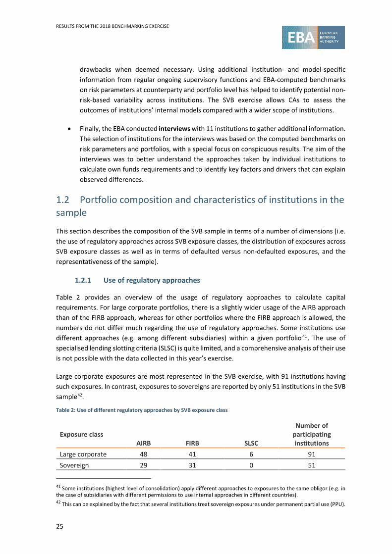
Table 2 provides an overview of the usage of regulatory approaches to calculate capital requirements. For large corporate portfolios, there is a slightly wider usage of the AIRB approach than of the FIRB approach, whereas for other portfolios where the FIRB approach is allowed, the numbers do not differ much regarding the use of regulatory approaches. Some institutions use different approaches (e.g. among different subsidiaries) within a given portfolio 41. The use of specialised lending slotting criteria (SLSC) is quite limited, and a comprehensive analysis of their use is not possible with the data collected in this year’s exercise.
Large corporate exposures are most represented in the SVB exercise, with 91 institutions having such exposures. In contrast, exposures to sovereigns are reported by only 51 institutions in the SVB sample42.
Table 2: Use of different regulatory approaches by SVB exposure class
Exposure class AIRB FIRB SLSC
Number of participating institutions
Large corporate 48 41 6 91 Sovereign 29 31 0 51
41 Some institutions (highest level of consolidation) apply different approaches to exposures to the same obligor (e.g. in the case of subsidiaries with different permissions to use internal approaches in different countries). 42 This can be explained by the fact that several institutions treat sovereign exposures under permanent partial use (PPU).
RESULTS FROM THE 2018 BENCHMARKING EXERCISE
26
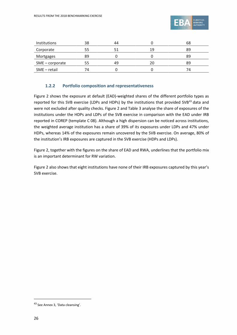
Institutions 38 44 0 68 Corporate 55 51 19 89 Mortgages 89 0 0 89 SME – corporate 55 49 20 89 SME – retail 74 0 0 74
1.2.2 Portfolio composition and representativeness
Figure 2 shows the exposure at default (EAD)-weighted shares of the different portfolio types as reported for this SVB exercise (LDPs and HDPs) by the institutions that provided SVB43 data and were not excluded after quality checks. Figure 2 and Table 3 analyse the share of exposures of the institutions under the HDPs and LDPs of the SVB exercise in comparison with the EAD under IRB reported in COREP (template C 08). Although a high dispersion can be noticed across institutions, the weighted average institution has a share of 39% of its exposures under LDPs and 47% under HDPs, whereas 14% of the exposures remain uncovered by the SVB exercise. On average, 80% of the institution’s IRB exposures are captured in the SVB exercise (HDPs and LDPs).
Figure 2, together with the figures on the share of EAD and RWA, underlines that the portfolio mix is an important determinant for RW variation.
Figure 2 also shows that eight institutions have none of their IRB exposures captured by this year’s SVB exercise.
43 See Annex 3, ‘Data cleansing’.

RESULTS FROM THE 2018 BENCHMARKING EXERCISE
27
Figure 2: Share of exposures under LDPs, under HDPs and outside the scope of the 2018 SVB exercise (comparison with total IRB portfolio from COREP data) (sorted by the share under LDPs from largest to smallest)
For 15 institutions, the SVB portfolio (LDPs and HDPs) captures less than 50% of the total EAD under the IRB approach. This highlights the scope of this exercise and the importance of other exposures not covered (e.g. credit card portfolios) in terms of total EADs under internal approaches. In addition, there are also other exposures that are not covered by the SVB exercise as they are under PPU (i.e. sovereign exposures, intragroup exposures, exposures belonging to an IPS, etc.).
Table 3: Summary statistics on the share of exposures under LDPs, under HDPs and outside the scope of the SVB exercise
Share of exposures
LDP HDP Other
Min. 0% 0% 0% 25th percentile 2% 29% 3% 50th percentile 13% 57% 9% 75th percentile 45% 85% 18% Max. 100% 100% 100%
Figure 3 shows the portfolio mix of all the participating institutions in the SVB exercise. The residential mortgages portfolio accounts for the largest share of the EAD exposures (32%) followed by the large corporates (20%). It is interesting to note that, in general, the LDPs and HDPs account for approximately 50% of the exposures, in terms of both EAD as well as RWA. As expected, the
0%
10%
20%
30%
40%
50%
60%
70%
80%
90%
100%
Share under LDP Share under HDP Share not in the SVB exercise (not HDP, not LDP)

RESULTS FROM THE 2018 BENCHMARKING EXERCISE
28
corporate exposure class (SME corporates, corporate-other, large corporates) is the riskiest, as its share of RWAs is highest when compared with its share of EAD (i.e. highest RW)44.
Figure 3: Portfolio composition of RWA (outer circle) and EAD (inner circle) for HDPs and LDPs (defaulted and non-defaulted)
Comparing Figure 3 and Table 3, quite a large discrepancy can be observed between the almost equal distribution of exposures between LDPs and HDPs in Figure 3, and Table 3, where 75% of institutions have a share of LDP exposures in the total amount of IRB exposures of less than 45%. From this it can be inferred that there is a relatively small share of large institutions (in terms of IRB exposures) that have the majority of their IRB exposures in LDPs.
Figure 4 shows how the exposures in the LDPs are distributed (in terms of share of exposures) among the different LDP SVB exposure classes, as reported by the 89 institutions that provided SVB
data on LDP exposures and were not excluded after quality checks. Similarly to in the LDP exercise in 2017, it can be seen that several institutions use the IRB approach exclusively for large corporates portfolios and do not have any exposures to institutions or sovereigns under the IRB approach. Very few institutions use the IRB approach only for institutions portfolios, none of them use the IRB approach only for sovereign portfolios.
44 This could be (partly) due to the fact that specialised lending exposures are part of the corporate exposure class, and are to be reported as such under the 2018 SVB ITS. This aspect has been rectified in the 2019 ITS.
20%
10%
15%
10%8%
5%
32%34%
9%
3%19%
14%
5%
16%
LCOR INST CGCB CORP
SMEC SMER MORT

RESULTS FROM THE 2018 BENCHMARKING EXERCISE
29
Figure 4: Portfolio composition of the LDPs: share of large corporates, institutions and sovereigns in LDPs (sorted by the share of large corporates in LDPs from largest to smallest)
Figure 5 shows how the exposures under the HDPs are distributed (in terms of share of exposures) among the different HDP SVB exposure classes, as reported by the 98 institutions that provided SVB
data and were not excluded after quality checks. The EAD distribution across the four HDPs shows that the exposure of the institutions is very diverse; some institutions are exposed to only one portfolio (residential mortgages, corporates-other or SME corporates), others to a mix of two or more portfolios.
0%
10%
20%
30%
40%
50%
60%
70%
80%
90%
100%
Share large corporates in LDP Share Institutions in LDP Share sovereigns in LDP
RESULTS FROM THE 2018 BENCHMARKING EXERCISE
30
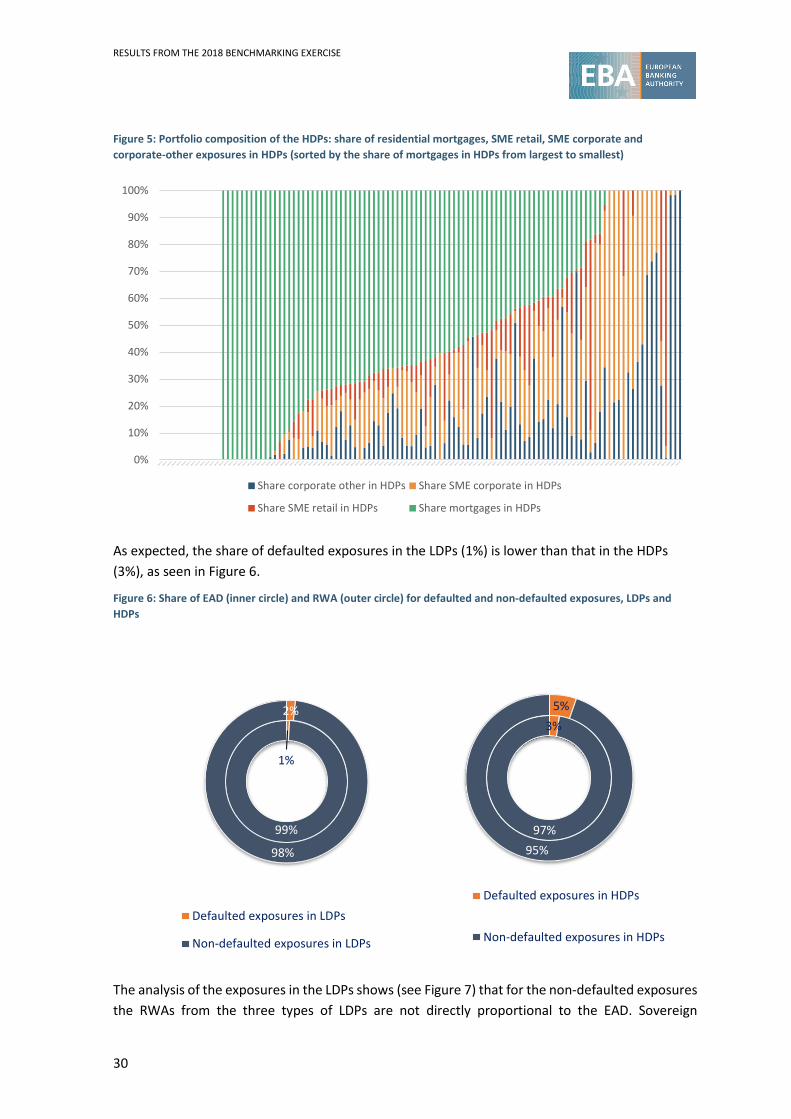
Figure 5: Portfolio composition of the HDPs: share of residential mortgages, SME retail, SME corporate and corporate-other exposures in HDPs (sorted by the share of mortgages in HDPs from largest to smallest)
As expected, the share of defaulted exposures in the LDPs (1%) is lower than that in the HDPs (3%), as seen in Figure 6.
Figure 6: Share of EAD (inner circle) and RWA (outer circle) for defaulted and non-defaulted exposures, LDPs and HDPs
The analysis of the exposures in the LDPs shows (see Figure 7) that for the non-defaulted exposures the RWAs from the three types of LDPs are not directly proportional to the EAD. Sovereign
0%
10%
20%
30%
40%
50%
60%
70%
80%
90%
100%
Share corporate other in HDPs Share SME corporate in HDPs
Share SME retail in HDPs Share mortgages in HDPs
1%
99%
2%
98%
Defaulted exposures in LDPs
Non-defaulted exposures in LDPs
3%
97%
5%
95%
Defaulted exposures in HDPs
Non-defaulted exposures in HDPs

RESULTS FROM THE 2018 BENCHMARKING EXERCISE
31
exposures represent 36% of the total EAD but only 8% of the total RWA. On the other hand, the large corporates portfolio shows a higher portion of RWAs compared with the EAD, i.e. it represents 43% of the total EAD and 76% of the total RWA. Figure 7 shows that most of the defaulted exposures stem, as expected, from the large corporates portfolios. Interestingly, the sovereign defaulted exposures do not attract any RWAs. This can be explained by the fact that the RW for defaulted exposures under the FIRB approach is zero (see Article 153(1)(ii) and Article 161(1) of the Capital Requirements Regulation (CRR)).
Figure 7: Share of EAD (inner circle) and RWA (outer circle) for defaulted and non-defaulted exposures by SVB portfolios (LDPs)
A similar conclusion can be drawn for the non-defaulted exposures in the HDPs in Figure 8, i.e. residential mortgage portfolios represent 60% of the total EAD but only 29% of the total RWA. On
94%
5%1%
98%
2%0%
Defaulted exposures largeCorporate
Defaulted exposures toinstitution
Defaulted exposures onsovereign
43%
21%
36%
76%
16%
8%Non-defaulted exposureslarge Corporate
Non-defaulted exposuresto institution
Non-defaulted exposureson sovereign

RESULTS FROM THE 2018 BENCHMARKING EXERCISE
32
the other hand, both SME corporates and SME retail portfolios show a higher proportion of RWAs compared with the EAD (e.g. SME corporate represents 14% of the total EAD and 26% of the total RWA).
Figure 8 shows the distribution of defaulted exposures across the different HDPs, with the lowest share in SME retail (16%), followed by corporates-other (24%), residential mortgages (32%) and the highest exposure in SME corporates (28%). However, the residential mortgages portfolio attracts most RWAs (39%).
Figure 8: Share of EAD (inner circle) and RWA (outer circle) for defaulted and non-defaulted exposures by SVB portfolios (HDPs)
24%
32%
28%
16%28%
39%
21%
12%Defaulted exposuresCorporate
Defaulted exposures toMortgages
Defaulted exposures onSMEC
Defaulted exposures onSMER
19%
60%
14%
7%37%
29%
26%
8%Non-defaulted exposuresCorporate
Non-defaulted exposures toMortgages
Non-defaulted exposures onSMEC
Non-defaulted exposures onSMER

RESULTS FROM THE 2018 BENCHMARKING EXERCISE
33
All in all, we see a wide variation of the share of exposures in the SVB exposure class levels among institutions and we see that the RWs vary greatly among SVB exposure classes and between defaulted and non-defaulted assets. This underlines the fact that the portfolio mix and the share of defaulted assets are important determinants of RW variation.

RESULTS FROM THE 2018 BENCHMARKING EXERCISE
34
2. Section 2: Quantitative analysis
2.1 Top-down and distribution analysis (LDPs and HDPs)
This section aims to determine and analyse the drivers behind RW variability across the institutions. In the top-down approach, two indicators are used to summarise the results of the variability: the GC45 (taking into account both expected loss (EL) and unexpected loss (UL)), and the RW (taking only UL into account). EL is important for many institutions and is influenced by IRB risk parameters, therefore the analysis of both components (EL and UL) provides useful information regarding the drivers of variability.
The top-down approach shows the extent to which the riskiness of portfolios (e.g. the portfolio composition) contributes to differences in average RW. However, a top-down approach does not explain the remaining differences (so-called ‘B type’ differences), i.e. if these differences stem from individual practices, interpretations of regulatory requirements, business strategies or modelling choices or if they are caused by other effects, such as idiosyncratic variations in the riskiness within an exposure class, CRM (i.e. the business and risk strategy of the institutions), and the estimation of IRB risk parameters (e.g. institutional46 and supervisory practices).
For the purpose of analysing drivers of differences in GC levels, a standard deviation index is calculated where the initial GC standard deviation is set at 100. ‘A-type’ differences in the present top-down analysis include the following:
• different relative shares of exposure classes (‘portfolio mix effect’); • different shares of defaulted exposures (‘default mix effect’); • the combined effects of different shares of defaulted exposures and different relative
shares of exposure classes.
This choice of differences is motivated by the facts that: • the portfolio mix and the share of default exposures are very different between institutions
(as presented in Figure 4 and Figure 5); • the differences of the distributions of GCs (as well as other variables such as RW, PD and
LGD) between the different default status (see Figure 9) and exposure classes (see RW dispersion in Annex 4) are remarkable.
45 The GC provides the information for both EL and UL for IRB exposures. For IRB exposures, it is computed as (12.5 × EL + RWA) ÷ EAD. For IRB, the RWA provides information only for UL. For SA defaulted exposures, it is computed as (12.5 × provisions + RWA) ÷ (exposure value + provision). For SA non-defaulted exposures, it is computed as (RWA ÷ exposure value). 46
For example, some institutions mentioned during the interviews that they update the ratings of their counterparties on an annual basis, while others update the ratings more frequently (e.g. three times a year); some institutions have a fixed period during the year for performing the updates (e.g. at the end of the first quarter of the year), whereas other institutions update the ratings during the year without a fixed period (e.g. because of time-consuming issues); some have semi-automatic procedures for downloading the financial statements of the counterparties, while other institutions perform the updates manually, and some outsource these updates.
RESULTS FROM THE 2018 BENCHMARKING EXERCISE
35
For a detailed comparison of these results to the previous exercises, see the temporal analysis in Section 2.4 of this report.
Methodology and assumptions
The methodology is broadly unchanged compared with previous years, although the analysis has been extended to control for additional factors. Annex 4 gives a comprehensive description of the analysis performed. This box briefly recaps the methodology through a simplified example.
In this example, the sample is composed of only three institutions and the factor analysed is the default mix (see Table 4).
Table 4: Example of the top-down approach
Institution 1 Institution 2 Institution 3 Total/average Example data GC_total 10% 20% 30% GC_def 30% 40% 55% GC_non def 5% 10% 5% EAD_total 50 120 20 Of which, EAD_def 10 40 10 Of which, EAD_non def 40 80 10
Computations % EAD_def 20% 33% 50% 60/190 = 32%
% EAD_non def 80% 67% 50% 130/190 = 68%
GC_total DEF NON DEF 13% 20% 21% Note: For the sake of clarity, the computation of GC_total DEF NON DEF for (for example) institution 1 is 32% × 30% + 68% × 5% = 13%). The standard deviations are computed using RW_total and RW_total DEF NON DEF. They are normalised by the standard deviation of RW_total to produce the graph with a starting point of 100.
2.1.1 Drivers of differences in GC
Taking into account all data from HDPs and LDPs together, the GC by institution varies significantly across the sample: the initial total GC standard deviation is 21%. The simple average total GC is 40%, the minimum is 7% and the maximum is 114%.
Considering only the LDPs, the simple average total GC is 41%, with a minimum of 7% and a maximum of 118%. Considering only the HDPs, the simple average total GC is 43%, with a minimum of 7% and a maximum of 137%.
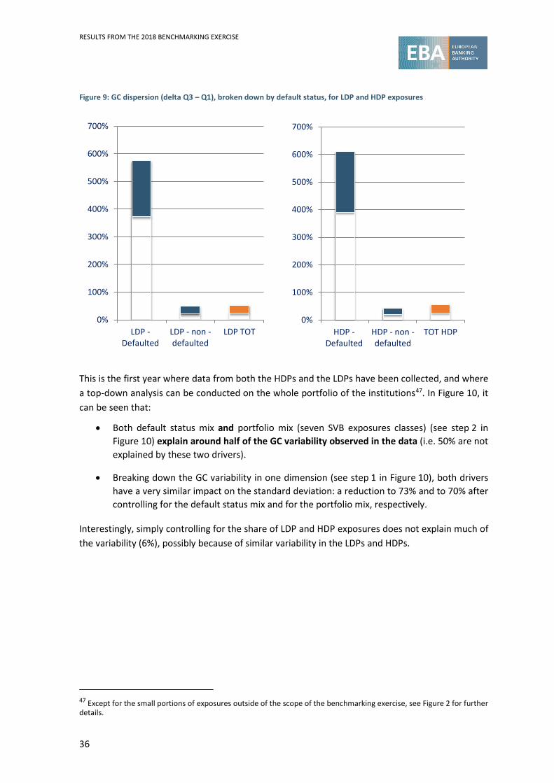
RESULTS FROM THE 2018 BENCHMARKING EXERCISE
36
Figure 9: GC dispersion (delta Q3 – Q1), broken down by default status, for LDP and HDP exposures
This is the first year where data from both the HDPs and the LDPs have been collected, and where a top-down analysis can be conducted on the whole portfolio of the institutions47. In Figure 10, it can be seen that:
• Both default status mix and portfolio mix (seven SVB exposures classes) (see step 2 in Figure 10) explain around half of the GC variability observed in the data (i.e. 50% are not explained by these two drivers).
• Breaking down the GC variability in one dimension (see step 1 in Figure 10), both drivers have a very similar impact on the standard deviation: a reduction to 73% and to 70% after controlling for the default status mix and for the portfolio mix, respectively.
Interestingly, simply controlling for the share of LDP and HDP exposures does not explain much of the variability (6%), possibly because of similar variability in the LDPs and HDPs.
47 Except for the small portions of exposures outside of the scope of the benchmarking exercise, see Figure 2 for further details.
0%
100%
200%
300%
400%
500%
600%
700%
LDP -Defaulted
LDP - non -defaulted
LDP TOT0%
100%
200%
300%
400%
500%
600%
700%
HDP -Defaulted
HDP - non -defaulted
TOT HDP

RESULTS FROM THE 2018 BENCHMARKING EXERCISE
37
Figure 10: Decomposition of the GC standard deviation index – HDPs and LDPs
Sample: 68 institutions, 14 variables in step 2 (default and portfolio mix (large corporate defaulted, large corporate non-defaulted, etc.) for each institution, 709 non-missing variables versus 243 missing variables for which the median values have been used. Note: When the GC is missing, it is assumed to be equal to the value of the benchmark. Figure 11 and Figure 12 visualise the top-down analysis for LDPs and HDPs separately. It can be seen from these figures that the share of variability that is unexplained by the default status mix and portfolio mix is again around half of the initial GC standard deviation index (44% for LDPs and 46% for HDPs). For LDPs, the portfolio mix is the greatest contributor to the reduction in the initial GC standard deviation index, whereas for HDPs and LDPs, the contribution of the default status mix and the portfolio mix is more or less equal.
100
73
50
100
70
50
-
20
40
60
80
100
120
Step 0. InitialGC STD
Step 1. (Default status mix)OR (Portfolio mix)
Step 2. (Default status mix)AND (Portfolio mix)
Step 1: Default status mix Step 1: Portfolio mix
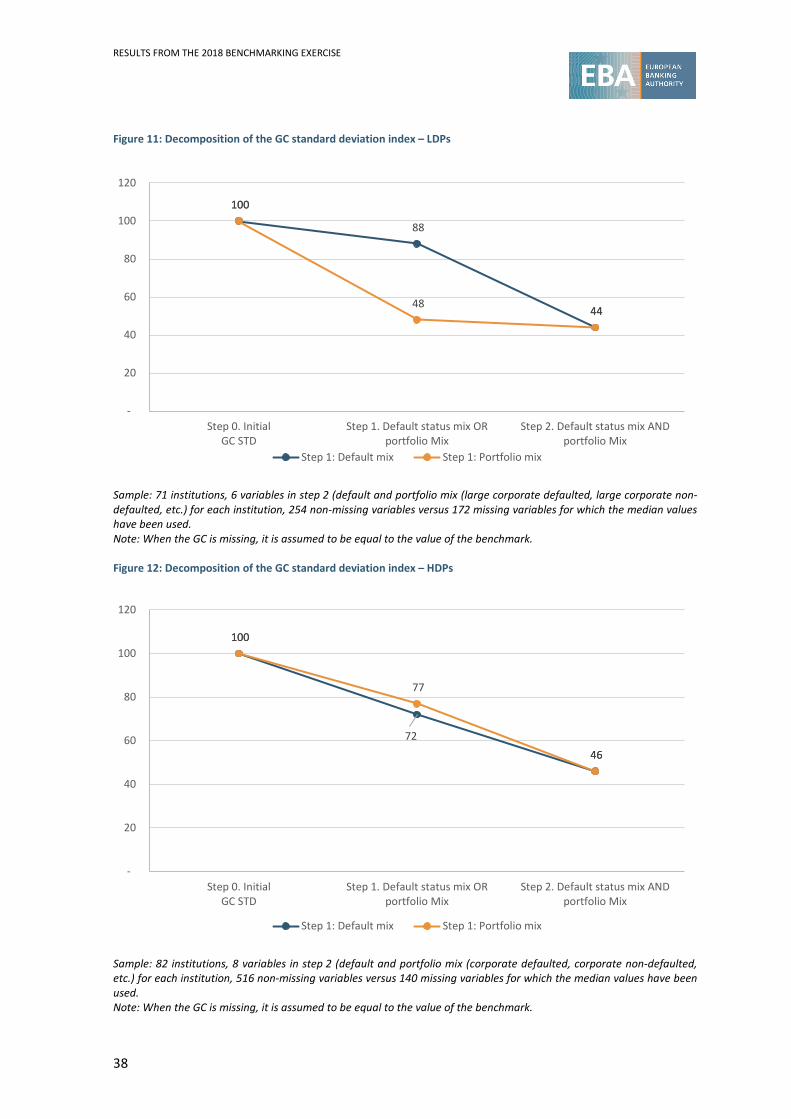
RESULTS FROM THE 2018 BENCHMARKING EXERCISE
38
Figure 11: Decomposition of the GC standard deviation index – LDPs
Sample: 71 institutions, 6 variables in step 2 (default and portfolio mix (large corporate defaulted, large corporate non-defaulted, etc.) for each institution, 254 non-missing variables versus 172 missing variables for which the median values have been used. Note: When the GC is missing, it is assumed to be equal to the value of the benchmark. Figure 12: Decomposition of the GC standard deviation index – HDPs
Sample: 82 institutions, 8 variables in step 2 (default and portfolio mix (corporate defaulted, corporate non-defaulted, etc.) for each institution, 516 non-missing variables versus 140 missing variables for which the median values have been used. Note: When the GC is missing, it is assumed to be equal to the value of the benchmark.
100
88
44
100
48 44
-
20
40
60
80
100
120
Step 0. InitialGC STD
Step 1. Default status mix ORportfolio Mix
Step 2. Default status mix ANDportfolio Mix
Step 1: Default mix Step 1: Portfolio mix
100
72 46
100
77
46
-
20
40
60
80
100
120
Step 0. InitialGC STD
Step 1. Default status mix ORportfolio Mix
Step 2. Default status mix ANDportfolio Mix
Step 1: Default mix Step 1: Portfolio mix

RESULTS FROM THE 2018 BENCHMARKING EXERCISE
39
In Section 2.4, this top-down analysis is compared with the top-down analysis of previous SVB exercises, i.e. the 2016 HDP exercise as well as the 2017 LDP exercise.
2.1.2 Impact of the top-down analysis on the GC and RW
Figure 13 shows the GC and RW for the overall LDPs and HDPs, and Figure 14 shows the adjusted figures after the top-down transformation has been done (at step 2, i.e. controlling for portfolio and default mix).
The reduction in variability in the GC and RW by controlling for the default status mix and the portfolio mix, can be seen by comparing Figure 13 with Figure 14, i.e. around half of the variability is eliminated by controlling for these known drivers of risk.
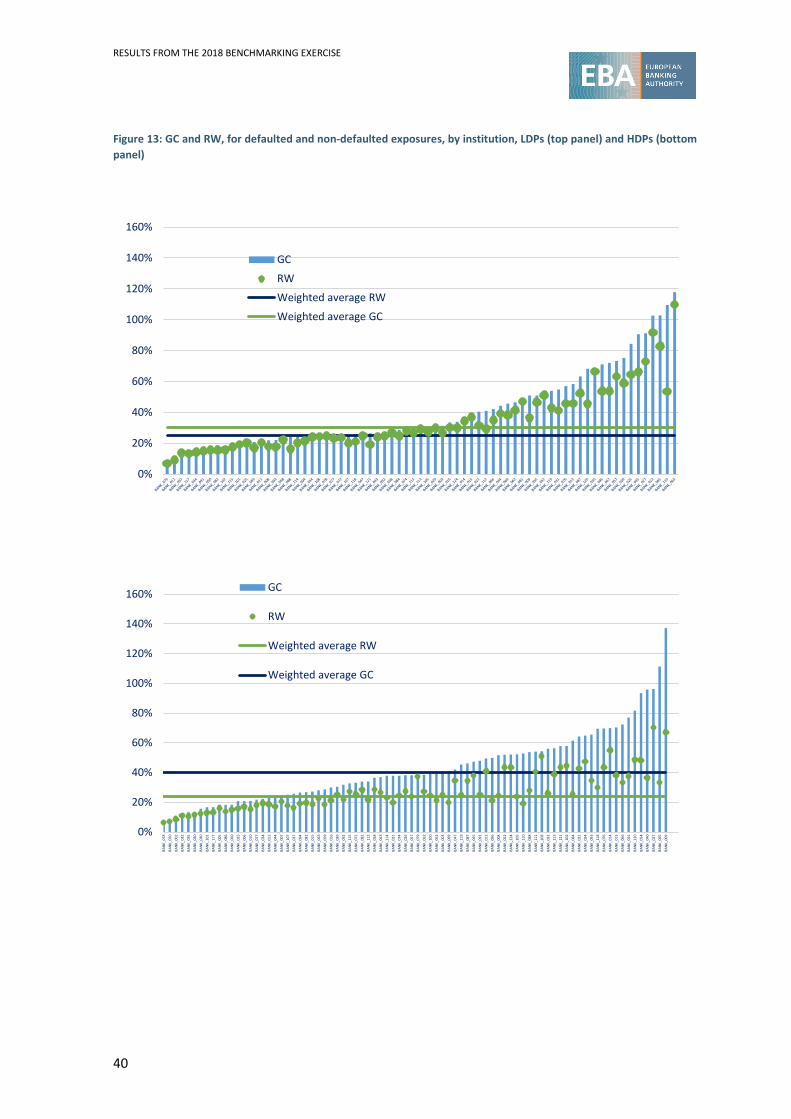
RESULTS FROM THE 2018 BENCHMARKING EXERCISE
40
Figure 13: GC and RW, for defaulted and non-defaulted exposures, by institution, LDPs (top panel) and HDPs (bottom panel)
0%
20%
40%
60%
80%
100%
120%
140%
160%
GC
RW
Weighted average RW
Weighted average GC
0%
20%
40%
60%
80%
100%
120%
140%
160%
BAN
K_07
8BA
NK_
050
BAN
K_00
2BA
NK_
032
BAN
K_03
5BA
NK_
020
BAN
K_03
0BA
NK_
101
BAN
K_11
7BA
NK_
005
BAN
K_08
6BA
NK_
060
BAN
K_02
5BA
NK_
006
BAN
K_01
0BA
NK_
077
BAN
K_03
4BA
NK_
012
BAN
K_04
4BA
NK_
007
BAN
K_10
7BA
NK_
037
BAN
K_09
4BA
NK_
081
BAN
K_01
5BA
NK_
063
BAN
K_05
9BA
NK_
016
BAN
K_03
9BA
NK_
092
BAN
K_11
5BA
NK_
072
BAN
K_08
2BA
NK_
112
BAN
K_05
8BA
NK_
043
BAN
K_11
4BA
NK_
021
BAN
K_07
4BA
NK_
026
BAN
K_05
7BA
NK_
079
BAN
K_06
2BA
NK_
100
BAN
K_06
1BA
NK_
003
BAN
K_06
9BA
NK_
047
BAN
K_11
9BA
NK_
087
BAN
K_04
5BA
NK_
091
BAN
K_01
1BA
NK_
096
BAN
K_00
8BA
NK_
052
BAN
K_12
4BA
NK_
105
BAN
K_11
0BA
NK_
088
BAN
K_11
1BA
NK_
108
BAN
K_03
1BA
NK_
113
BAN
K_12
1BA
NK_
102
BAN
K_08
4BA
NK_
022
BAN
K_02
4BA
NK_
093
BAN
K_11
8BA
NK_
076
BAN
K_01
4BA
NK_
013
BAN
K_06
6BA
NK_
055
BAN
K_12
0BA
NK_
054
BAN
K_04
0BA
NK_
027
BAN
K_06
5BA
NK_
009
GC
RW
Weighted average RW
Weighted average GC

RESULTS FROM THE 2018 BENCHMARKING EXERCISE
41
Figure 14: Adjusted GC and RW, for defaulted and non-defaulted exposures, by institution, LDPs (top panel) and HDPs (bottom panel)
0%
20%
40%
60%
80%
100%
120%
140%
160%
BAN
K_07
8BA
NK_
050
BAN
K_00
2BA
NK_
032
BAN
K_03
5BA
NK_
020
BAN
K_03
0BA
NK_
101
BAN
K_11
7BA
NK_
005
BAN
K_08
6BA
NK_
060
BAN
K_02
5BA
NK_
006
BAN
K_01
0BA
NK_
077
BAN
K_03
4BA
NK_
012
BAN
K_04
4BA
NK_
007
BAN
K_10
7BA
NK_
037
BAN
K_09
4BA
NK_
081
BAN
K_01
5BA
NK_
063
BAN
K_05
9BA
NK_
016
BAN
K_03
9BA
NK_
092
BAN
K_11
5BA
NK_
072
BAN
K_08
2BA
NK_
112
BAN
K_05
8BA
NK_
043
BAN
K_11
4BA
NK_
021
BAN
K_07
4BA
NK_
026
BAN
K_05
7BA
NK_
079
BAN
K_06
2BA
NK_
100
BAN
K_06
1BA
NK_
003
BAN
K_06
9BA
NK_
047
BAN
K_11
9BA
NK_
087
BAN
K_04
5BA
NK_
091
BAN
K_01
1BA
NK_
096
BAN
K_00
8BA
NK_
052
BAN
K_12
4BA
NK_
105
BAN
K_11
0BA
NK_
088
BAN
K_11
1BA
NK_
108
BAN
K_03
1BA
NK_
113
BAN
K_12
1BA
NK_
102
BAN
K_08
4BA
NK_
022
BAN
K_02
4BA
NK_
093
BAN
K_11
8BA
NK_
076
BAN
K_01
4BA
NK_
013
BAN
K_06
6BA
NK_
055
BAN
K_12
0BA
NK_
054
BAN
K_04
0BA
NK_
027
BAN
K_06
5BA
NK_
009
HDP - GC Adjusted
HDP - RW Adjusted
Weighted average GC
WAVG RW adjusted
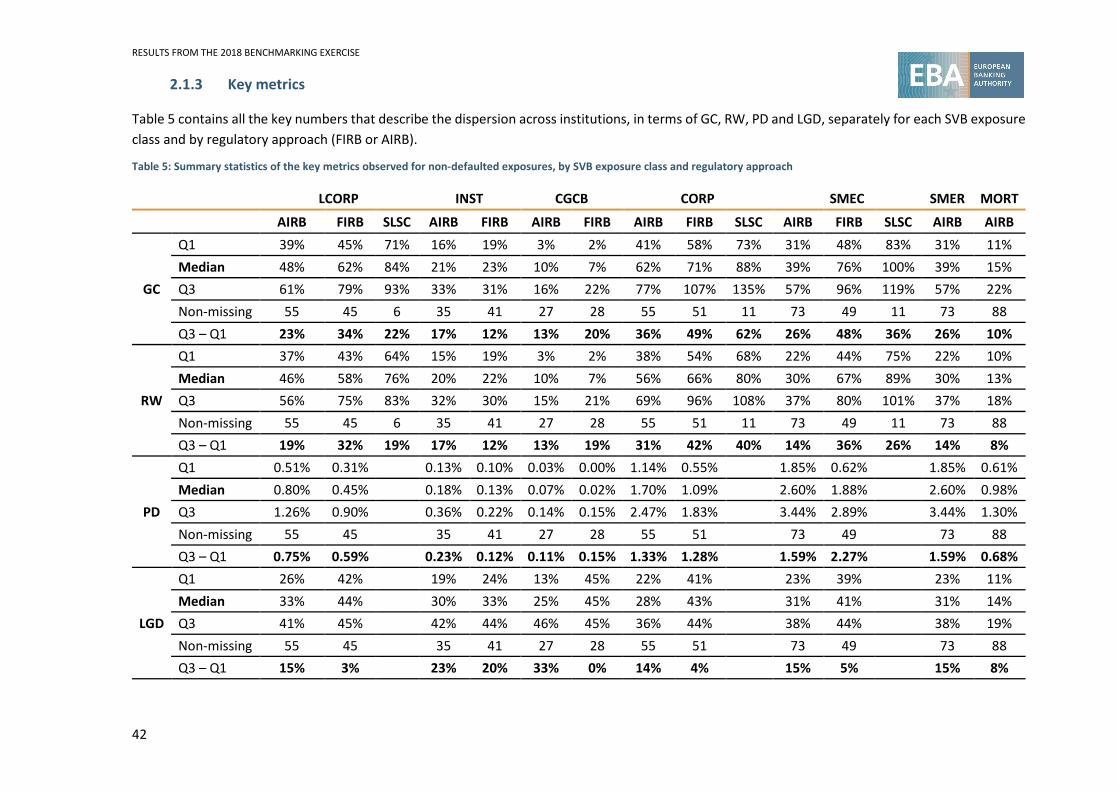
RESULTS FROM THE 2018 BENCHMARKING EXERCISE
42
2.1.3 Key metrics
Table 5 contains all the key numbers that describe the dispersion across institutions, in terms of GC, RW, PD and LGD, separately for each SVB exposure class and by regulatory approach (FIRB or AIRB).
Table 5: Summary statistics of the key metrics observed for non-defaulted exposures, by SVB exposure class and regulatory approach
LCORP INST CGCB CORP SMEC SMER MORT
AIRB FIRB SLSC AIRB FIRB AIRB FIRB AIRB FIRB SLSC AIRB FIRB SLSC AIRB AIRB
GC
Q1 39% 45% 71% 16% 19% 3% 2% 41% 58% 73% 31% 48% 83% 31% 11% Median 48% 62% 84% 21% 23% 10% 7% 62% 71% 88% 39% 76% 100% 39% 15% Q3 61% 79% 93% 33% 31% 16% 22% 77% 107% 135% 57% 96% 119% 57% 22% Non-missing 55 45 6 35 41 27 28 55 51 11 73 49 11 73 88 Q3 – Q1 23% 34% 22% 17% 12% 13% 20% 36% 49% 62% 26% 48% 36% 26% 10%
RW
Q1 37% 43% 64% 15% 19% 3% 2% 38% 54% 68% 22% 44% 75% 22% 10% Median 46% 58% 76% 20% 22% 10% 7% 56% 66% 80% 30% 67% 89% 30% 13% Q3 56% 75% 83% 32% 30% 15% 21% 69% 96% 108% 37% 80% 101% 37% 18% Non-missing 55 45 6 35 41 27 28 55 51 11 73 49 11 73 88 Q3 – Q1 19% 32% 19% 17% 12% 13% 19% 31% 42% 40% 14% 36% 26% 14% 8%
PD
Q1 0.51% 0.31% 0.13% 0.10% 0.03% 0.00% 1.14% 0.55% 1.85% 0.62% 1.85% 0.61% Median 0.80% 0.45% 0.18% 0.13% 0.07% 0.02% 1.70% 1.09% 2.60% 1.88% 2.60% 0.98% Q3 1.26% 0.90% 0.36% 0.22% 0.14% 0.15% 2.47% 1.83% 3.44% 2.89% 3.44% 1.30% Non-missing 55 45 35 41 27 28 55 51 73 49 73 88 Q3 – Q1 0.75% 0.59% 0.23% 0.12% 0.11% 0.15% 1.33% 1.28% 1.59% 2.27% 1.59% 0.68%
LGD
Q1 26% 42% 19% 24% 13% 45% 22% 41% 23% 39% 23% 11% Median 33% 44% 30% 33% 25% 45% 28% 43% 31% 41% 31% 14% Q3 41% 45% 42% 44% 46% 45% 36% 44% 38% 44% 38% 19% Non-missing 55 45 35 41 27 28 55 51 73 49 73 88 Q3 – Q1 15% 3% 23% 20% 33% 0% 14% 4% 15% 5% 15% 8%

RESULTS FROM THE 2018 BENCHMARKING EXERCISE
43
2.2 Analysis of IRB parameters for common counterparties (LDPs)
The purpose of this analysis is to compare institutions’ IRB parameters for a common set of counterparties, and to try to explain the remaining B-type differences. This analysis was also performed for the 2015 and the 2017 report on LDP exposures and the methodology remained unchanged. It should be noted that this analysis does not take into account the specific exposure of the institutions (e.g. collateral in LGD effect) and hence results have to be treated with care.
Institutions were instructed to provide risk parameters for a predefined list of obligors (where the institution has an exposure for these obligors). This allowed a direct comparison of the IRB parameters and resulting RW for a set of identical common counterparties, even if real exposures might differ as a result of different CRM techniques and/or collateralisation schemes.
The RW for each participating institution was compared with the benchmark to better understand the effects and importance of the various drivers. The benchmark used was the RW median for the group of institutions that apply the same regulatory approach to a specific common counterparty. An obligor under the FIRB approach is therefore compared with the FIRB benchmark, and an obligor under the AIRB approach is compared with the AIRB benchmark for that counterparty.
To isolate the impact of each IRB parameter, the RWs are recalculated, at obligor level, using various combinations of actual and benchmark parameters. By replacing an institution’s risk parameter with a benchmark parameter (median risk parameter), it is possible to disentangle the different effects of each parameter individually: the PD effect and maturity effect are analysed for obligors under both approaches (AIRB and FIRB), while the LGD effect and the hypothetical LGD effect are only analysed for obligors under AIRB, as the FIRB approach defines a regulatory LGD of 45% for senior unsecured exposures and hence no deviation from this level may be expected. Analysis of obligors under the FIRB approach separate from obligors under the AIRB approach ensures that findings, in particular as regards PD and LGD, are not affected by differences in underlying approaches.
Methodology and assumptions
The comprehensive description of the analysis can be found in Annex 4. For the reader’s convenience, the main features of the analysis are given below:
• Deviation 1 (initial RW deviation): 𝑫𝑫𝑫𝑫𝑫𝑫𝑫𝑫 = 𝑹𝑹𝑹𝑹(𝑴𝑴,𝑷𝑷𝑫𝑫,𝑳𝑳𝑳𝑳𝑫𝑫) −𝑹𝑹𝑹𝑹(𝟐𝟐.𝟓𝟓,𝑷𝑷𝑫𝑫𝒃𝒃𝑫𝑫𝒃𝒃𝒃𝒃𝒃𝒃𝒃𝒃𝒃𝒃𝒃𝒃𝒃𝒃,𝑳𝑳𝑳𝑳𝑫𝑫𝒃𝒃𝑫𝑫𝒃𝒃𝒃𝒃𝒃𝒃𝒃𝒃𝒃𝒃𝒃𝒃𝒃𝒃)
• Deviation 2 (PD effect): 𝑫𝑫𝑫𝑫𝑫𝑫𝟐𝟐 = 𝑹𝑹𝑹𝑹(𝟐𝟐.𝟓𝟓,𝑷𝑷𝑫𝑫,𝑳𝑳𝑳𝑳𝑫𝑫𝒃𝒃𝑫𝑫𝒃𝒃𝒃𝒃𝒃𝒃𝒃𝒃𝒃𝒃𝒃𝒃𝒃𝒃)− 𝑹𝑹𝑹𝑹(𝟐𝟐.𝟓𝟓,𝑷𝑷𝑫𝑫𝒃𝒃𝑫𝑫𝒃𝒃𝒃𝒃𝒃𝒃𝒃𝒃𝒃𝒃𝒃𝒃𝒃𝒃,𝑳𝑳𝑳𝑳𝑫𝑫𝒃𝒃𝑫𝑫𝒃𝒃𝒃𝒃𝒃𝒃𝒃𝒃𝒃𝒃𝒃𝒃𝒃𝒃)
• Deviation 3 (LGD effect): 𝑫𝑫𝑫𝑫𝑫𝑫𝑫𝑫 = 𝑹𝑹𝑹𝑹(𝟐𝟐.𝟓𝟓,𝑷𝑷𝑫𝑫𝒃𝒃𝑫𝑫𝒃𝒃𝒃𝒃𝒃𝒃𝒃𝒃𝒃𝒃𝒃𝒃𝒃𝒃,𝑳𝑳𝑳𝑳𝑫𝑫)− 𝑹𝑹𝑹𝑹(𝟐𝟐.𝟓𝟓,𝑷𝑷𝑫𝑫𝒃𝒃𝑫𝑫𝒃𝒃𝒃𝒃𝒃𝒃𝒃𝒃𝒃𝒃𝒃𝒃𝒃𝒃,𝑳𝑳𝑳𝑳𝑫𝑫𝒃𝒃𝑫𝑫𝒃𝒃𝒃𝒃𝒃𝒃𝒃𝒃𝒃𝒃𝒃𝒃𝒃𝒃)
• Deviation 4 (maturity effect): 𝑫𝑫𝑫𝑫𝑫𝑫𝑫𝑫 = 𝑹𝑹𝑹𝑹(𝑴𝑴,𝑷𝑷𝑫𝑫𝒃𝒃𝑫𝑫𝒃𝒃𝒃𝒃𝒃𝒃𝒃𝒃𝒃𝒃𝒃𝒃𝒃𝒃,𝑳𝑳𝑳𝑳𝑫𝑫𝒃𝒃𝑫𝑫𝒃𝒃𝒃𝒃𝒃𝒃𝒃𝒃𝒃𝒃𝒃𝒃𝒃𝒃)− 𝑹𝑹𝑹𝑹(𝟐𝟐.𝟓𝟓,𝑷𝑷𝑫𝑫𝒃𝒃𝑫𝑫𝒃𝒃𝒃𝒃𝒃𝒃𝒃𝒃𝒃𝒃𝒃𝒃𝒃𝒃,𝑳𝑳𝑳𝑳𝑫𝑫𝒃𝒃𝑫𝑫𝒃𝒃𝒃𝒃𝒃𝒃𝒃𝒃𝒃𝒃𝒃𝒃𝒃𝒃) • Deviation 5 (LGD effect without CRM effect, i.e. on hypothetical unsecured LGD):

RESULTS FROM THE 2018 BENCHMARKING EXERCISE
44
𝑫𝑫𝑫𝑫𝑫𝑫𝟓𝟓 = 𝑹𝑹𝑹𝑹�𝟐𝟐.𝟓𝟓,𝑷𝑷𝑫𝑫𝒃𝒃𝑫𝑫𝒃𝒃𝒃𝒃𝒃𝒃𝒃𝒃𝒃𝒃𝒃𝒃𝒃𝒃,𝑳𝑳𝑳𝑳𝑫𝑫𝒃𝒃𝒉𝒉𝒉𝒉 𝒖𝒖𝒃𝒃𝒖𝒖𝑫𝑫𝒃𝒃� − 𝑹𝑹𝑹𝑹�𝟐𝟐.𝟓𝟓,𝑷𝑷𝑫𝑫𝒃𝒃𝑫𝑫𝒃𝒃𝒃𝒃𝒃𝒃𝒃𝒃𝒃𝒃𝒃𝒃𝒃𝒃,𝑳𝑳𝑳𝑳𝑫𝑫𝒃𝒃𝑫𝑫𝒃𝒃𝒃𝒃𝒃𝒃𝒃𝒃𝒃𝒃𝒃𝒃𝒃𝒃𝒃𝒃𝒉𝒉𝒉𝒉 𝒖𝒖𝒃𝒃𝒖𝒖𝑫𝑫𝒃𝒃 �
One limitation of this approach is that it does not take into account regulatory measures (such as add-ons) currently in place at RWA level. Hence, for some institutions in jurisdictions where such supervisory measures are in place, the recomputed RWAs are not directly comparable with the RWAs actually held and/or reported by the institutions. There are also additional factors that may have an impact on such benchmarking (e.g. point in time (PIT), versus through the cycle (TTC); default definition; last update of the ratings; scope of the rating system), but these aspects are an integral part of the analysis and should be carefully analysed for the identified outlier institutions.
Furthermore, as mentioned in Section 1, the subset of common counterparties may not be not be fully representative of the total IRB portfolio of the individual institutions, therefore the results of this exercise may not be transferable to the total IRB portfolios and should be interpreted with care. Figure 15 shows that, generally speaking, the C 101.00 sample makes up a small part of the institutions’ IRB EAD. This figure shows all observations as dots. The median is displayed as a red diamond and the whiskers denote the range between the first and the third quartile.
Figure 15: LDP common counterparties compared with corresponding IRB EAD or RWA from COREP data
For each institution and each of its counterparties, the RW deviation resulting from substituting the risk parameters with their benchmark is computed and the findings can be summarised as follows:
Most of the interquartile ranges of the deviations resulting from benchmark substitutions are below 10%, with a slightly higher variability for AIRB institutions in the large corporates portfolio (partially explained by the higher PD variability). In particular, there seems to be no
0%
20%
40%
60%
80%
100%
% EAD
LCORP INST SOV ALL0%
20%
40%
60%
80%
100%
% RWA
LCORP INST SOV ALL

RESULTS FROM THE 2018 BENCHMARKING EXERCISE
45
significant difference in the variability between AIRB and FIRB institutions on the institutions and the sovereign portfolios.
There are strong non-linearity effects, i.e. the variability of the different risk parameters is compensating to some extent (the total deviation is well below the sum of the deviation of each risk parameter): in short, low PD estimates are generally associated with high LGD estimates, and vice versa.
Table 6 shows the summary statistics (1st and 3rd quartile, median and interquartile range) of the RW deviations by SVB exposure class and regulatory approach, whereas
Figure 16 to Figure 18 visualise the deviations of the institutions for large corporate exposures, sovereigns and institutions.
Table 6: Summary statistics on the RW deviations (1st and 3rd quartile, median and interquartile range) by SVB exposure class and regulatory approach
AIRB FIRB
Dev 1 (ALL)
Dev2 (PD)
Dev3 (LGD)
Dev4 Dev5 (LGDunsec)
Dev 1 (ALL)
Dev2 (PD) (M)
Large corporates Q1 -7.73% -3.65% -5.97% -4.89% -5.73% -1.77% -2.10% Q3 4.48% 5.10% 2.47% 1.53% 2.98% 5.47% 2.92% median -1.06% 1.06% -0.64% -0.64% 0.00% 0.01% 0.00% Q3 -Q1 12.21% 8.75% 8.43% 6.42% 8.72% 7.24% 5.02% Sovereigns Q1 -5.83% -2.66% -4.60% -2.82% -3.99% -1.66% -1.40% Q3 2.32% 3.03% 1.82% 4.98% 0.74% 4.11% 4.25% median -1.31% 0.93% -1.12% -0.98% -0.27% 0.00% 0.00% Q3 -Q1 8.15% 5.70% 6.42% 7.80% 4.73% 5.77% 5.65% Institutions Q1 -8.70% -0.41% -6.17% -8.25% -3.81% -7.70% -2.85% Q3 0.11% 3.44% 2.52% -2.83% 2.09% 0.00% 3.06% median -5.28% 0.06% 0.02% -6.30% 0.00% -2.66% 0.00% Q3 -Q1 8.82% 3.85% 8.69% 5.42% 5.90% 7.70% 5.90%
The interquartile differences are greater under the AIRB approach than under the FIRB approach for large corporate exposures and sovereigns. For the large corporate exposures, this difference is the greatest, i.e. the interquartile range is 12.21% under the AIRB versus 7.24% under the FIRB (i.e. a difference of almost 5 percentage points).
In the AIRB, the interquartile difference of the RW deviation is greatest for large corporate exposures. This stems from the fact that the variability introduced by the PD and the unsecured LGD is greatest for large corporate exposures. The interquartile range for sovereign exposures and exposures to institutions seems to be lower than for the large corporate portfolios.
The interquartile range of the LGD effect is highest for large corporates and institutions (above 8%) and lowest for sovereign exposures (6.42%). The analysis for sovereign exposures must, however,
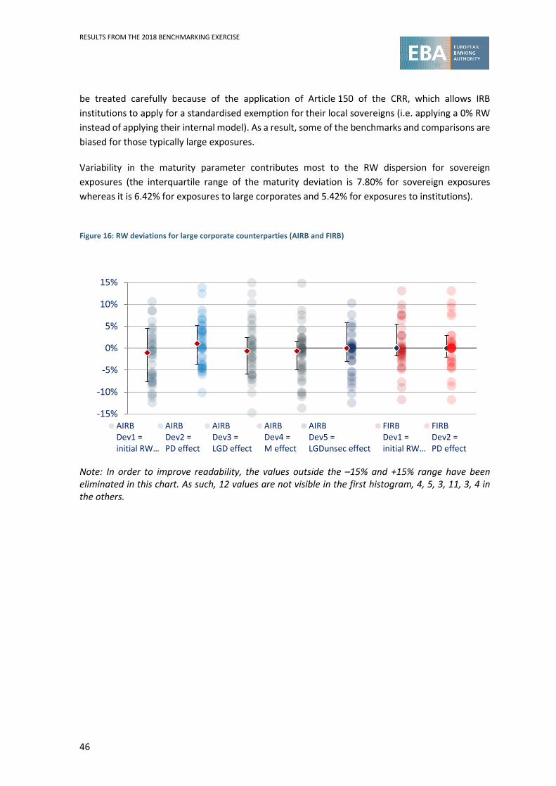
RESULTS FROM THE 2018 BENCHMARKING EXERCISE
46
be treated carefully because of the application of Article 150 of the CRR, which allows IRB institutions to apply for a standardised exemption for their local sovereigns (i.e. applying a 0% RW instead of applying their internal model). As a result, some of the benchmarks and comparisons are biased for those typically large exposures.
Variability in the maturity parameter contributes most to the RW dispersion for sovereign exposures (the interquartile range of the maturity deviation is 7.80% for sovereign exposures whereas it is 6.42% for exposures to large corporates and 5.42% for exposures to institutions).
Figure 16: RW deviations for large corporate counterparties (AIRB and FIRB)
Note: In order to improve readability, the values outside the –15% and +15% range have been eliminated in this chart. As such, 12 values are not visible in the first histogram, 4, 5, 3, 11, 3, 4 in the others.
-15%
-10%
-5%
0%
5%
10%
15%
AIRBDev1 =initial RW…
AIRBDev2 =PD effect
AIRBDev3 =LGD effect
AIRBDev4 =M effect
AIRBDev5 =LGDunsec effect
FIRBDev1 =initial RW…
FIRBDev2 =PD effect

RESULTS FROM THE 2018 BENCHMARKING EXERCISE
47
Figure 17: Dispersion of RW deviations, by regulatory approach – sovereigns
Note: In order to improve readability, the values outside the –15% and +15% range have been eliminated in this chart. As such, 2 values are not visible in the first histogram, 3, 3, 1, 7, 0, 0 in the others. Figure 18: Dispersion of RW deviations, by regulatory approach – institutions
Note: In order to improve readability, the values outside the –15% and +15% range have been eliminated in this chart. As such, 2 values are not visible in the first histogram, 1, 1, 1, 3, 1, 0 in the others.
2.3 Outturns (backtesting) approaches (HDPs)
-15%
-10%
-5%
0%
5%
10%
15%
AIRBDev1 =initial RW…
AIRBDev2 =PD effect
AIRBDev3 =LGD effect
AIRBDev4 =M effect
AIRBDev5 =LGDunsec effect
FIRBDev1 =initial RW…
FIRBDev2 =PD effect
-15%
-10%
-5%
0%
5%
10%
15%
AIRBDev1 =initial RW…
AIRBDev2 =PD effect
AIRBDev3 =LGD effect
AIRBDev4 =M effect
AIRBDev5 =LGDunsec effect
FIRBDev1 =initial RW…
FIRBDev2 =PD effect

RESULTS FROM THE 2018 BENCHMARKING EXERCISE
48
In contrast to the exercise for LDPs, for HDPs it is not possible to compare the same counterparties across institutions. Instead, it is possible to control for some of the key features of exposures. In particular, historical data on defaulted exposures, i.e. default rates and loss rates, are an important source of information on the portfolio risk as they allow a kind of backtesting (outturns approach). This approach is very useful since the misalignment between estimates (PDs and LGDs) and observed parameters (default rates and loss rates) could suggest that differences in RWAs across institutions might be driven by differences in estimation practices (e.g. different levels of conservatism, adjustments to reflect long-run averages, different lengths of time series of the data available and included in the calibration of the cycle, assumptions underlying recovery estimates, etc.) and not only by differences in portfolio risk.
Methodology and assumptions
The comprehensive description of the analysis can be found in Annex 4. For the reader’s convenience, its main features are given below. Using the information provided by institutions in accordance with the ITS, it is possible to compare, for the same institution and across institutions, the estimated parameters with the observed parameters, namely the following indicators:
• Estimated parameters (IRB parameters)48: PD and LGD.
• Observed49 parameters: the default rate for the past year50, the average default rate for the past 5 years, the loss rate for the past year51 and the average loss rate for the past 5 years.
• Backtesting results:
o RWA*, which is the hypothetical RWA that results from the application of the maximum of PD and p*. For each counterparty grade, 𝐩𝐩∗ is the smallest positive value satisfying the equation:
𝐩𝐩∗ + 𝚽𝚽−𝑫𝑫(𝐪𝐪) ∙ �𝐩𝐩∗ ∙ (𝑫𝑫 − 𝐩𝐩∗)
𝐧𝐧≥ 𝐃𝐃𝐃𝐃𝑫𝑫𝟏𝟏
o and RWA**, which is similar to RWA*, but using the 𝐃𝐃𝐃𝐃𝟓𝟓𝟏𝟏 instead of 𝐃𝐃𝐃𝐃𝑫𝑫𝟏𝟏.
48 Parameters used for RWA calculation excluding the effect of potential measures introduced in accordance with Article 458 of Regulation (EU) No 575/2013. 49 Contrary to the default rate, the loss rate is not ‘purely’ observed, as it includes credit risk adjustments that have been estimated by the institution (see footnote 51) 50 The default rate for last year, in this exercise, is the ratio of (i) the sum of the exposures (at December 2016) that defaulted in 2017 to (ii) the sum of the exposures that were non-defaulted at December 2016. 51 The loss rate for the last year, in this exercise, is the ratio of (i) the sum of credit risk adjustments and write-offs applied, within 2017, to exposures that were non-defaulted at December 2016 and that defaulted during 2017 to (ii) the sum of the EAD, measured at December 2016, of the exposures that were non-defaulted at December 2016 and that defaulted during 2017.

RESULTS FROM THE 2018 BENCHMARKING EXERCISE
49
The persistence of institutions as outliers for both periods, i.e. 1-year rate and the average of the past 5 years, and across comparable parameters can be examined by the CAs. However, there are a couple of caveats that should be kept in mind when doing this comparison, in particular for the comparison at the risk parameters level (see the comprehensive list in Annex 4):
• Differences between the observed risk parameters used for prudential purposes and the data collected (default weighted versus exposure weighted).
• Differences between the rates collected and the long-run averages. PD and LGD estimates are required by Articles 180 and 181 of the CRR to be representative (PD) or at least equal (LGD) to the long-run average. However, the collected observed average values are not fully adequate (representativeness of the variations of the cycle, arithmetic versus exposure weighted average, grade level versus segment level).
• Differences between the long-run averages and the risk parameters (MoC, downturn).
Moreover, the data collected allowed only the comparison of PDs at the reference date (2017) with the default rate observed during the previous year (2016 – and also an average of the past 5 years), whereas it would be more consistent to compare this default rate with the PD at the beginning of the observation period. This is not optimal and so the results provide only a test for outliers, whereas further analysis should be done by the CA in order to assess whether the differences are risk- or practice-based.
There are also weaknesses in the backtesting of the LGD with the loss rate as, contrary to the default rate, the loss rate is not truly observed as it accounts for both observed losses and estimated credit risk adjustments. Accordingly, an LR/LGD ratio higher than 100% does not reflect, per se, a lack of conservatism: it could be because of a difference in the estimation of LGD and credit risk adjustments.
The RWA* and RWA** impact analysis also has a number of caveats:
• The two metrics aim to provide only an estimate of the potential magnitude of RWA changes under a specific scenario influenced by observed parameters (a one-sided view).
• The two metrics do not reflect regulatory measures or corrective actions in place that are having an impact on institutions’ capital requirements.
• Extrapolations to the total IRB credit risk portfolio cannot be made, because of the specific nature of HDP exposures.
The figures in Table 7 show that the hypothetical RWAs are equal to the observed RWAs for at least half of the institutions. Looking at the third quartile values, it can be noted that the variability within the AIRB portfolios is higher than that within the FIRB institutions for the same portfolios, especially when looking at the RWA* (which is determined by the default rate for the past year). In general however, the variability remains relatively low. Overall, this backtesting analysis does not reveal a material negative deviation of the estimated level of risk compared with the observed level for the vast majority of the EU institutions.
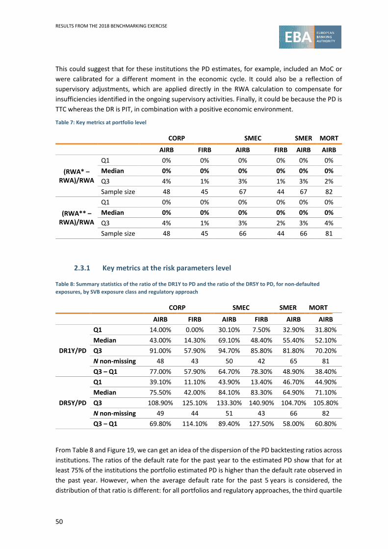
RESULTS FROM THE 2018 BENCHMARKING EXERCISE
50
This could suggest that for these institutions the PD estimates, for example, included an MoC or were calibrated for a different moment in the economic cycle. It could also be a reflection of supervisory adjustments, which are applied directly in the RWA calculation to compensate for insufficiencies identified in the ongoing supervisory activities. Finally, it could be because the PD is TTC whereas the DR is PIT, in combination with a positive economic environment.
Table 7: Key metrics at portfolio level
CORP SMEC SMER MORT
AIRB FIRB AIRB FIRB AIRB AIRB
(RWA* – RWA)/RWA
Q1 0% 0% 0% 0% 0% 0% Median 0% 0% 0% 0% 0% 0% Q3 4% 1% 3% 1% 3% 2% Sample size 48 45 67 44 67 82
(RWA** – RWA)/RWA
Q1 0% 0% 0% 0% 0% 0% Median 0% 0% 0% 0% 0% 0% Q3 4% 1% 3% 2% 3% 4% Sample size 48 45 66 44 66 81
2.3.1 Key metrics at the risk parameters level
Table 8: Summary statistics of the ratio of the DR1Y to PD and the ratio of the DR5Y to PD, for non-defaulted exposures, by SVB exposure class and regulatory approach
CORP SMEC SMER MORT
AIRB FIRB AIRB FIRB AIRB AIRB
DR1Y/PD
Q1 14.00% 0.00% 30.10% 7.50% 32.90% 31.80% Median 43.00% 14.30% 69.10% 48.40% 55.40% 52.10% Q3 91.00% 57.90% 94.70% 85.80% 81.80% 70.20% N non-missing 48 43 50 42 65 81 Q3 – Q1 77.00% 57.90% 64.70% 78.30% 48.90% 38.40%
DR5Y/PD
Q1 39.10% 11.10% 43.90% 13.40% 46.70% 44.90% Median 75.50% 42.00% 84.10% 83.30% 64.90% 71.10% Q3 108.90% 125.10% 133.30% 140.90% 104.70% 105.80% N non-missing 49 44 51 43 66 82 Q3 – Q1 69.80% 114.10% 89.40% 127.50% 58.00% 60.80%
From Table 8 and Figure 19, we can get an idea of the dispersion of the PD backtesting ratios across institutions. The ratios of the default rate for the past year to the estimated PD show that for at least 75% of the institutions the portfolio estimated PD is higher than the default rate observed in the past year. However, when the average default rate for the past 5 years is considered, the distribution of that ratio is different: for all portfolios and regulatory approaches, the third quartile

RESULTS FROM THE 2018 BENCHMARKING EXERCISE
51
of the empirical distribution is above 100%. In general, the interquartile range of the DR5Y/PD ratio is higher than the interquartile range of the DR1Y/PD, except for corporate-other exposures in the AIRB.
When the results for different regulatory approaches are compared for the ratio of the 5-year default rate to the PD estimate, it is observed that the variability is higher for FIRB portfolios than for AIRB portfolios.
Finally, the comparison of the backtesting results across different SVB exposure classes, shows that the variability is higher for corporates (SME and others) than for retail portfolios.
Figure 19: Interquartile range of the ratio of DR1Y to PD and the ratio of DR5Y to PD, for non-defaulted exposures, by SVB exposure class and regulatory approach
Table 9: Interquartile range of the ratio of LR1Y to LGD and the ratio of LR5Y to LGD, for non-defaulted exposures, by SVB exposure class and regulatory approach
CORP SMEC SMER MORT
AIRB FIRB AIRB FIRB AIRB AIRB
LR1Y/LGD
Q1 0.10% 0.00% 0.60% 0.00% 2.20% 1.60% Median 30.10% 0.50% 45.60% 13.20% 47.40% 32.40% Q3 82.60% 42.30% 81.90% 62.30% 84.30% 73.00% N non-missing 47 39 48 38 64 78 Q3 – Q1 82.50% 42.30% 81.20% 62.30% 82.10% 71.30%
LR5Y/LGD
Q1 0.40% 0.00% 1.10% 0.30% 2.70% 4.60% Median 29.40% 9.00% 30.50% 19.80% 43.20% 31.70% Q3 80.50% 49.10% 61.30% 56.30% 75.40% 61.60% N non-missing 47 41 48 42 64 79 Q3 – Q1 80.20% 49.10% 60.20% 56.00% 72.80% 57.00%

RESULTS FROM THE 2018 BENCHMARKING EXERCISE
52
From Table 9 and Figure 20, we can gain an overview of the ratio of the loss rate (1-year and 5-year) to the LGD estimate across institutions. The ratio between the loss rate and the estimated LGD shows that for at least 75% of the institutions the portfolio estimated LGD is higher than the loss rate observed in the past year or in the past 5 years, which means that the LGDs reported by the institutions are generally higher than the loss rates for the past 5 years. In contrast to the PD backtesting results, the interquartile range of the LR5Y/LGD ratio is usually lower than the interquartile range of the LR1Y/LGD ratio. Furthermore, the third quartile is lower for all SVB exposure classes, except for corporates under FIRB.
It can also be observed that the first quartile, for all the distributions, is very close to zero. This is possibly due to a problem in the reporting of the loss rates or in data quality issues.
Figure 20: Range of the ratio of LR1Y to LGD and the ratio of LR5Y to LGD, for non-defaulted exposures, by portfolio and regulatory approach

RESULTS FROM THE 2018 BENCHMARKING EXERCISE
53
2.4 Temporal analysis
This section contains a comparison of this year’s SVB results with those of the previous exercises, i.e. the 2016 HDP and 2017 LDP results. In particular, the top-down analysis, the common counterparty analysis and the backtesting results are compared with those of the previous exercises.
2.4.1 General statistics
For this review of parameters over time, a sample of common institutions (institutions that participated in the 2016, 2017 and 2018 exercises) was created, resulting in a sample of 69 institutions. All the figures presented in here are replicated in Annex 5, with a breakdown by regulatory approach (AIRB and FIRB).
An increase in the EAD can be noticed from EUR 12.3 to EUR 13.5 trillion (see Figure 21)52.
Figure 21: Common EAD among the 2016, 2017 and 2018 SVB exercises (EUR millions)
Figure 22 shows the evolution of the (EAD-weighted average) PD and LGD, as well as the RW across SVB exercises. It can be noted that the average parameter estimates and RW are fairly stable over time.
52 Key messages from the split per regulatory approach (Annex 5): no significant difference. The increase of sovereign exposures mainly comes from FIRB exposures.
1,808,998
1,323,459
2,434,095
1,002,065
949,124
591,941
4,203,644
2,042,981
1,352,860
2,791,423
1,421,454
1,049,551
637,042
4,212,758
0 500,000 1,000,000 1,500,000 2,000,000 2,500,000 3,000,000 3,500,000 4,000,000 4,500,000
Sovereigns
Institutions
Large Corporates
Corporate Other
SME Corporate
SME Retail
Retail Mortgage
EAD 2018 EAD Previous BM
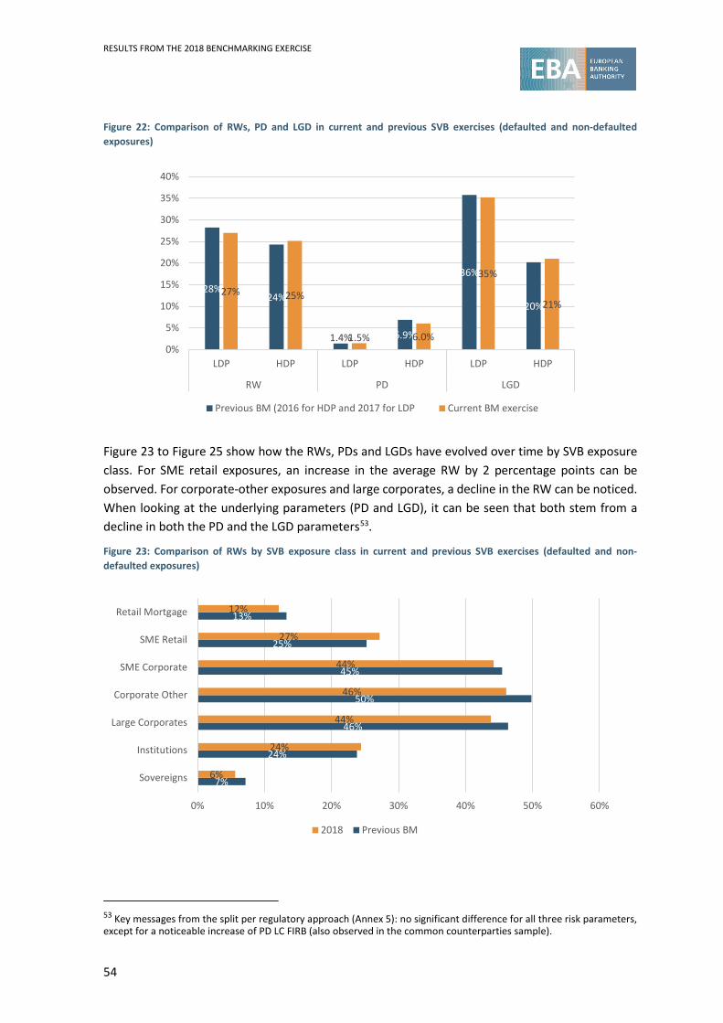
RESULTS FROM THE 2018 BENCHMARKING EXERCISE
54
Figure 22: Comparison of RWs, PD and LGD in current and previous SVB exercises (defaulted and non-defaulted exposures)
Figure 23 to Figure 25 show how the RWs, PDs and LGDs have evolved over time by SVB exposure class. For SME retail exposures, an increase in the average RW by 2 percentage points can be observed. For corporate-other exposures and large corporates, a decline in the RW can be noticed. When looking at the underlying parameters (PD and LGD), it can be seen that both stem from a decline in both the PD and the LGD parameters53.
Figure 23: Comparison of RWs by SVB exposure class in current and previous SVB exercises (defaulted and non-defaulted exposures)
53 Key messages from the split per regulatory approach (Annex 5): no significant difference for all three risk parameters, except for a noticeable increase of PD LC FIRB (also observed in the common counterparties sample).
28%24%
1.4% 6.9%
36%
20%27% 25%
1.5% 6.0%
35%
21%
0%
5%
10%
15%
20%
25%
30%
35%
40%
LDP HDP LDP HDP LDP HDP
RW PD LGD
Previous BM (2016 for HDP and 2017 for LDP Current BM exercise
7%
24%
46%
50%
45%
25%
13%
6%
24%
44%
46%
44%
27%
12%
0% 10% 20% 30% 40% 50% 60%
Sovereigns
Institutions
Large Corporates
Corporate Other
SME Corporate
SME Retail
Retail Mortgage
2018 Previous BM

RESULTS FROM THE 2018 BENCHMARKING EXERCISE
55
Figure 24: Comparison of PDs by SVB exposure class in current and previous SVB exercises (defaulted and non-defaulted exposures)
Figure 25: Comparison of LGDs by SVB exposure class in current and previous SVB exercises (defaulted and non-defaulted exposures)
2.4.2 Top-down analysis
In the top-down analysis, Figure 26 shows that a lower share of the GC variability can be explained by known drivers over time. In particular, after controlling for differences in the default mix and portfolio mix, there is still 47% of GC variability left, as compared with 39% in last year’s analysis. The same pattern has been observed in the 2017 SVB exercise report, in its comparison of the 2017 exercise with the 2015 exercise, i.e. only 33% of GC variability remained in the 201554 exercise after
54 The results of the 2015 SVB exercise should be interpreted with caution as this was the pilot exercise and was based on a limited sample of institutions.
0%
1%
3%
9%
17%
14%
3%
0%
0%
3%
6%
14%
13%
3%
0% 2% 4% 6% 8% 10% 12% 14% 16% 18%
Sovereigns
Institutions
Large Corporates
Corporate Other
SME Corporate
SME Retail
Retail Mortgage
2018 Previous BM
34%
32%
39%
32%
31%
30%
14%
33%
34%
38%
30%
31%
30%
14%
0% 5% 10% 15% 20% 25% 30% 35% 40% 45%
Sovereigns
Institutions
Large Corporates
Corporate Other
SME Corporate
SME Retail
Retail Mortgage
2018 Previous BM
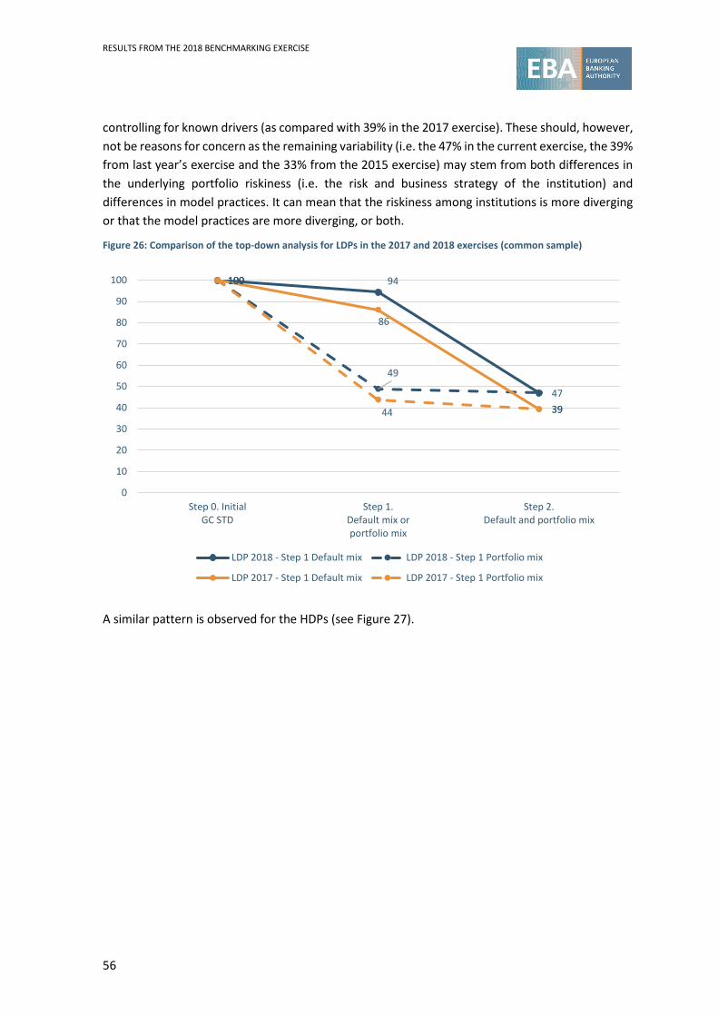
RESULTS FROM THE 2018 BENCHMARKING EXERCISE
56
controlling for known drivers (as compared with 39% in the 2017 exercise). These should, however, not be reasons for concern as the remaining variability (i.e. the 47% in the current exercise, the 39% from last year’s exercise and the 33% from the 2015 exercise) may stem from both differences in the underlying portfolio riskiness (i.e. the risk and business strategy of the institution) and differences in model practices. It can mean that the riskiness among institutions is more diverging or that the model practices are more diverging, or both.
Figure 26: Comparison of the top-down analysis for LDPs in the 2017 and 2018 exercises (common sample)
A similar pattern is observed for the HDPs (see Figure 27).
100 94
47
49
100
86
39
100
44 39
0
10
20
30
40
50
60
70
80
90
100
Step 0. InitialGC STD
Step 1.Default mix orportfolio mix
Step 2.Default and portfolio mix
LDP 2018 - Step 1 Default mix LDP 2018 - Step 1 Portfolio mix
LDP 2017 - Step 1 Default mix LDP 2017 - Step 1 Portfolio mix

RESULTS FROM THE 2018 BENCHMARKING EXERCISE
57
Figure 27: Comparison of the top-down analysis for HDPs in the 2016 and 2018 exercises (common sample)
It is also insightful to assess the standard deviation of the GC over time. Taking into account all data from HDPs and LDPs together, the initial total GC standard deviation is 21%. The simple average total GC is 40%, whereas the minimum is 7% and the maximum is 114%.
Considering only the LDPs, the simple average total GC is 41%, with a minimum of 7% and a maximum of 118%. The initial total GC standard deviation in LDPs is 26%, which is lower than the initial standard deviation of the GC as computed for the 2017 LDP exercise (when it was 33%).
Considering only the HDPs, the simple average total GC is 43%, with a minimum of 7% and a maximum of 137%. The initial total GC standard deviation in HDPs is 24%, which is considerably lower than the initial standard deviation of the GC as computed for the 2016 HDP exercise (when it was 82%).
From the decrease in the initial GC standard deviation, it can not be concluded that there is an improvement in the consistency of GC, as the GC standard deviation stems both from differences in institution’s modelling practices and from risk-taking behaviour. That is, the decrease in GC standard deviation appears to suggest that there is greater consistency in institutions’ internal model outcomes, but this does not hold true: the reduction in GC standard deviation may stem from a greater consistency in risk-taking behaviour (for instance consistency in loan granting and therefore in portfolio composition). It could even mean that internal model outcomes are increasingly more diverse, in case institutions’ risk-taking behaviour is converging and outweighing the practice-based differences.
76 74
45
100
62
28
65
0
10
20
30
40
50
60
70
80
90
100
Step 0. InitialGC STD
Step 1.Default mix orportfolio mix
Step 2.Default and portfolio mix
HDP 2018 - Step 1 Default mix HDP 2018 - Step 1 Portfolio mix
HDP 2016 - Step 1 Default mix HDP 2016 - Step 1 Portfolio mix

RESULTS FROM THE 2018 BENCHMARKING EXERCISE
58
2.4.3 LDP exercises
This section compares the common counterparty analysis with that of 2017 (end of 2016 data). The amount of exposures covered by the common counterparty analysis (for LDPs), is considerably low compared with the total scope of the SVB analysis, i.e. EUR 2.3 trillion are in the scope of the common counterparty analysis, compared with EUR 13.5 trillion captured in the portfolio analysis of both HDPs and LDPs55.
Comparison of the samples of counterparties
For this analysis, a common subsample of 73 institutions has been identified (i.e. institutions which participated in both exercises with an exposure in at least one SVB exposure class). It should however be noted that the number of institutions for each SVB exposure class is not the same, as well as the number of counterparties (see Figure 28). The comparison focused on a subset of counterparties that were reported by at least five institutions in both LDP exercises. Figure 28 shows the evolution of the total size of subset of counterparties in terms of EAD. Overall, the size is rather stable, which is explained by the few changes in the participating institutions and list of counterparties56. As shown in Annex 4, the EAD is also stable at the level of the SVB exposure class, but with a slight increase in the proportion of EAD under FIRB approach (this tendency would have to be confirmed in future report, in particular for exposures to sovereign counterparties).
Figure 28: Share of EAD in the common subsample
Figure 29 shows the evolution of the (exposure-weighted average) RW, PD and LGD on the common counterparties by SVB exposure class, separately for the FIRB and AIRB approach. In general, the average RW, PD and LGD estimates have remained relatively stable between the 2017 and the 2018 exercises, with the exception being the PD for large corporates under the FIRB (this pattern can also
55 Data being reported under template C 102 and C 103. 56 As mentioned in the previous report, the comparison is less relevant with the exercise conducted in 2015 as the changes done were more significant.
100%93%
87%
0%
10%
20%
30%
40%
50%
60%
70%
80%
90%
100%
2018 (all) 2018 (subsample) 2017 (subsample)

RESULTS FROM THE 2018 BENCHMARKING EXERCISE
59
be seen in Figure 56), which increased from 0.55% to 1.39%, as well as the PD for large corporates under AIRB, which increased from 1% up to 1.37%. Across SVB exercises, the PD for sovereign exposures is quite low, but is considerably higher in the AIRB (0.11%) than in the FIRB approach (0.025%). For the LGD estimates, the opposite pattern can be observed, i.e. the LGD for sovereign exposures under the AIRB approach is considerably lower than the LGD under the FIRB approach (around 27% versus 44% respectively). Since these parameters affect the RW in opposite directions, there is no consistent difference in the RW across the regulatory approach over the two SVB exercises.
Figure 29: Evolution of the common subsample from the 2015 LDP exercise to the 2017 LDP exercise, by SVB exposure class
Comparison of the observed variability
0.0%0.2%0.4%0.6%0.8%1.0%1.2%1.4%1.6%
Previous Current
PD (EAD weighted)
LCORP - AIRB LCORP - FIRB
INST - AIRB INST - FIRB
CGCB - AIRB CGCB - FIRB
0%
10%
20%
30%
40%
50%
60%
Previous Current
LGD (EAD weighted)
LCORP - AIRB LCORP - FIRB
INST - AIRB INST - FIRB
CGCB - AIRB CGCB - FIRB
0%
10%
20%
30%
40%
50%
Previous Current
RW (EAD weighted)
LCORP - AIRB LCORP - FIRB
INST - AIRB INST - FIRB
CGCB - AIRB CGCB - FIRB
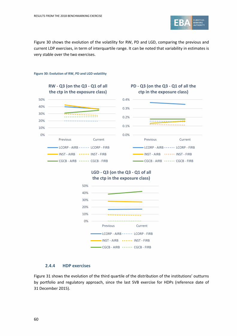
RESULTS FROM THE 2018 BENCHMARKING EXERCISE
60
Figure 30 shows the evolution of the volatility for RW, PD and LGD, comparing the previous and current LDP exercises, in term of interquartile range. It can be noted that variability in estimates is very stable over the two exercises.
Figure 30: Evolution of RW, PD and LGD volatility
2.4.4 HDP exercises
Figure 31 shows the evolution of the third quartile of the distribution of the institutions’ outturns by portfolio and regulatory approach, since the last SVB exercise for HDPs (reference date of 31 December 2015).
0%
10%
20%
30%
40%
50%
Previous Current
RW - Q3 (on the Q3 - Q1 of all the ctp in the exposure class)
LCORP - AIRB LCORP - FIRB
INST - AIRB INST - FIRB
CGCB - AIRB CGCB - FIRB
0.0%
0.1%
0.2%
0.3%
0.4%
Previous Current
PD - Q3 (on the Q3 - Q1 of all the ctp in the exposure class)
LCORP - AIRB LCORP - FIRB
INST - AIRB INST - FIRB
CGCB - AIRB CGCB - FIRB
0%
10%
20%
30%
40%
50%
Previous Current
LGD - Q3 (on the Q3 - Q1 of all the ctp in the exposure class)
LCORP - AIRB LCORP - FIRB
INST - AIRB INST - FIRB
CGCB - AIRB CGCB - FIRB

RESULTS FROM THE 2018 BENCHMARKING EXERCISE
61
Figure 31: Default rate to PD ratio trend
Regarding the ratios of the default rate to the PD, both for the past year and for the past 5 years, a clear decreasing trend can be seen. Considering that DRs are usually more PIT than PD, which are more TTC, this could be a reflection of a general improvement in economic conditions. This is in line with the fact that the ratios of the default rate to the PD are, for almost all portfolios, lower when based on default rates from the past year than when based on those from the past 5 years.
One can observe that the estimated PDs for all portfolios are higher than the observed default rates for the past year, which was not the case in 2015 for corporates-other under the FIRB approach or for SME corporate and SME retail under the AIRB approach. There was a big decrease in the backtesting results for corporates-other under the FIRB approach (from around 150% to 50%) which suggests not only that the default rates have decreased but also that the PDs may have been adjusted, reflecting in their calibration the higher historical default rates.
With respect to the 5-year average, the results are quite stable. An opposite trend is observable in the results for corporates under FIRB approach (slight increase, staying above 100%).
0%
50%
100%
150%
200%
Previous Current
DR1Y / PD - trend Q3
CORP - AIRB CORP - FIRB
MORT - AIRB SMER - AIRB
SMEC - AIRB SMEC - FIRB
0%
50%
100%
150%
200%
Previous Current
DR5Y/PD - trend Q3
CORP - AIRB CORP - FIRB
MORT - AIRB SMER - AIRB
SMEC - AIRB SMEC - FIRB

RESULTS FROM THE 2018 BENCHMARKING EXERCISE
62
Figure 32: Loss rate to LGD ratio trend
The backtesting results regarding the LGDs and the observed loss rates show a similar tendency, that is, in general, the ratios have decreased since 2015, and the ratios computed using the observed data for the past 5 years are more stable than those computed using the observed data for the past year. The results for SME corporate under the FIRB approach are the exception in that they show an increasing trend when the loss rate for the past year is compared with the LGD. The fact that the ratio of the 5-year average loss rate to the LGD is similar for 2015 and 2017 suggests that the LGD estimates have been adjusted since 2015.
Figure 33: RWA** and RWA* versus RWA trend
In line with the tendency of the outturns for PD (DR1Y/PD and DR5Y/PD), the difference between the RWA* and RWA and between RWA** and RWA either decreased or was maintained since the last exercise. Again, the exception to this is the tendency for corporate-other under the AIRB approach that shows an increase from December 2015 to December 2017 with regard to RWA*, and corporate-other under the FIRB approach with regard to RWA**.
0%
20%
40%
60%
80%
100%
120%
Previous Current
LR1Y/LGD - trend Q3
CORP - AIRB CORP - FIRB
MORT - AIRB SMER - AIRB
SMEC - AIRB SMEC - FIRB
0%
20%
40%
60%
80%
100%
120%
Previous Current
LR5Y/LGD - trend Q3
CORP - AIRB CORP - FIRB
MORT - AIRB SMER - AIRB
SMEC - AIRB SMEC - FIRB
-1%
4%
9%
14%
Previous Current
(RWA* - RWA)/RWA - trend Q3
CORP - AIRB CORP - FIRB
MORT - AIRB SMER - AIRB
SMEC - AIRB SMEC - FIRB
0%
5%
10%
15%
Previous Current
(RWA** - RWA)/RWA - trend Q3
CORP - AIRB CORP - FIRB
MORT - AIRB SMER - AIRB
SMEC - AIRB SMEC - FIRB
RESULTS FROM THE 2018 BENCHMARKING EXERCISE
63
3. Section 3: Qualitative analysis
3.1 Competent authorities’ assessments
Article 78(4) of the CRD requires CAs to make an assessment where institutions diverge significantly from the majority of their peers or where there is little commonality in approaches leading to a wide variance in results. In these cases, the CA should investigate the reasons and take corrective action if the institution’s approach leads to an underestimation of own funds requirements that is not attributable to differences in the underlying risks. In order to facilitate the transfer of the information gathered in these assessments from the CAs to the EBA, the EBA issued a questionnaire to the CAs, which had to be completed for each institution participating in the SVB exercise. The EBA received the responses for 105 institutions. This section summarises the key information derived from these assessments.
Figure 34 shows the CA’s overall assessment of the level of institution’s own funds requirements considering benchmark deviations for the different SVB exposure classes57. It should be noted that, even though some deviations in the outcomes of the internal model are observed compared with the benchmarks, the number of unjustified negative deviations is, on average, (across SVB exposure classes) limited to 15% of the institutions with a material exposure58.
57 Note that those cases where the institution does not have material exposures have been left out of this chart.
58 In some cases, the CA indicated that it is not possible to know the effect on the institution’s own funds requirements. Some of the reasons relate to data quality issues, or it is mentioned that a negative deviation of the PD may be compensated by a positive deviation of the LGD, or because the relevant portfolio covers only a small fraction of exposures under the SVB exposure class, or because it is hard to make general statements for the SVB exposure classes as the institution has several models (with diverging assessments) for (some of) the SVB exposure classes.

RESULTS FROM THE 2018 BENCHMARKING EXERCISE
64
Figure 34: CA’s overall assessment of the level of institutions’ own funds requirements, taking into account benchmark deviations
In roughly half of the institutions for which justified deviations have been identified in the SVB exercise, the deviations in RWs are linked with the risk and business strategy of the institution, which generally holds true for all SVB exposure classes (see Figure 35). More specifically, CAs refer to the specific structure of the institution’s portfolio (for instance covered bonds or the inclusion of shipping specialised lending exposures59 in the corporate portfolios), but the risk strategy and business strategy of the institution is also said to be related to the lending strategy of the institution, which may translate into the long-run average default rate and the LTV ratios of the portfolio and to the collateralisation rates of the portfolio, which in turn translate into the recovery rates.
59 Note that this (the separation of specialised lending exposures) has been revised in the ITS for the 2019 benchmarking exercise (https://www.eba.europa.eu/-/eba-publishes-updated-its-package-for-2019-benchmarking-exercise ).
38
34
45
47
46
38
47
42
39
45
5
6
14
14
16
10
12
11
8
13
8
24
18
16
18
15
21
17
17
18
0
1
0
0
0
1
0
0
0
0
0
0
2
2
0
1
1
1
1
1
0% 10% 20% 30% 40% 50% 60% 70% 80% 90% 100%
Sovereigns
Institutions
Large Corporates
Corporate Other
SME Corporate
SME Retail
Retail Mortgage
AVERAGE
AVERAGE LDP
AVERAGE HDP
In line with the benchmarks Negative deviations not justified
Negative deviations justified Positive deviations not justified
Positive deviations justified
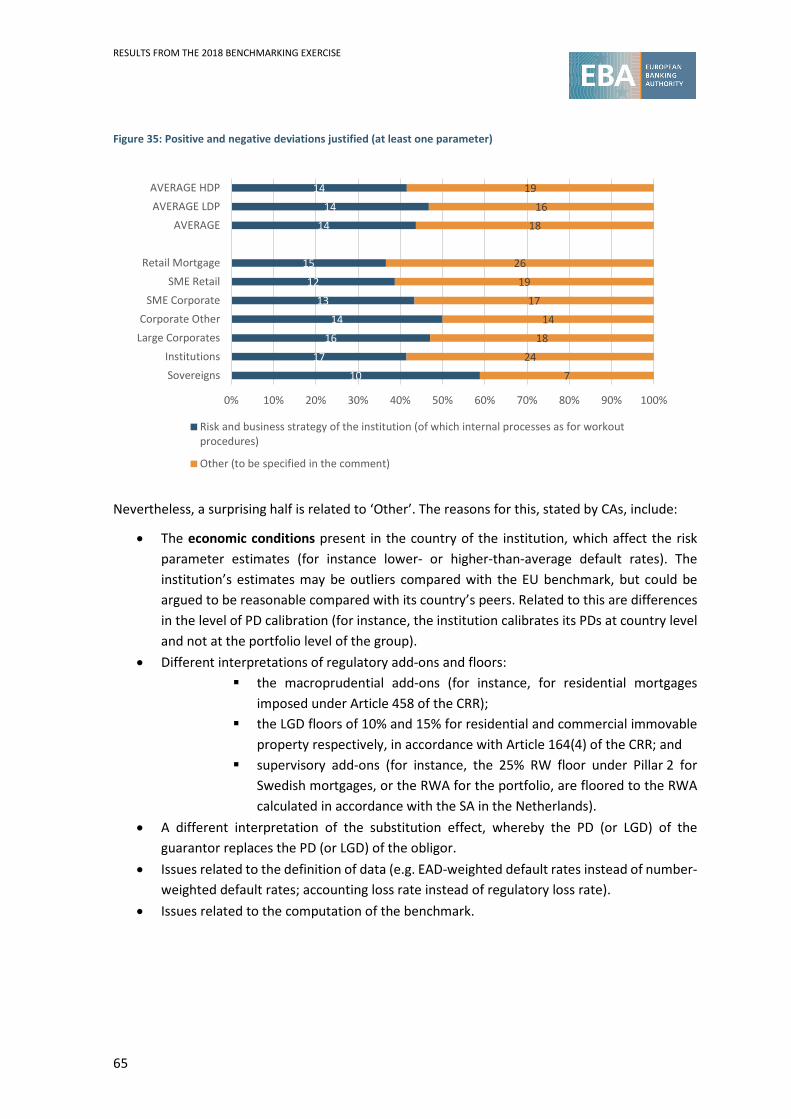
RESULTS FROM THE 2018 BENCHMARKING EXERCISE
65
Figure 35: Positive and negative deviations justified (at least one parameter)
Nevertheless, a surprising half is related to ‘Other’. The reasons for this, stated by CAs, include:
• The economic conditions present in the country of the institution, which affect the risk parameter estimates (for instance lower- or higher-than-average default rates). The institution’s estimates may be outliers compared with the EU benchmark, but could be argued to be reasonable compared with its country’s peers. Related to this are differences in the level of PD calibration (for instance, the institution calibrates its PDs at country level and not at the portfolio level of the group).
• Different interpretations of regulatory add-ons and floors: the macroprudential add-ons (for instance, for residential mortgages
imposed under Article 458 of the CRR); the LGD floors of 10% and 15% for residential and commercial immovable
property respectively, in accordance with Article 164(4) of the CRR; and supervisory add-ons (for instance, the 25% RW floor under Pillar 2 for
Swedish mortgages, or the RWA for the portfolio, are floored to the RWA calculated in accordance with the SA in the Netherlands).
• A different interpretation of the substitution effect, whereby the PD (or LGD) of the guarantor replaces the PD (or LGD) of the obligor.
• Issues related to the definition of data (e.g. EAD-weighted default rates instead of number-weighted default rates; accounting loss rate instead of regulatory loss rate).
• Issues related to the computation of the benchmark.
1017
1614
1312
15
1414
14
724
1814
1719
26
1816
19
0% 10% 20% 30% 40% 50% 60% 70% 80% 90% 100%
SovereignsInstitutions
Large CorporatesCorporate Other
SME CorporateSME Retail
Retail Mortgage
AVERAGEAVERAGE LDPAVERAGE HDP
Risk and business strategy of the institution (of which internal processes as for workoutprocedures)
Other (to be specified in the comment)

RESULTS FROM THE 2018 BENCHMARKING EXERCISE
66
Figure 36: Common reasons for negative deviations not justified (at least one parameter)
Figure 36 breaks down the different reasons causing unjustified underestimations identified by CAs. ‘Problems with the calibration of the risk parameters’ slightly leads as the main reason, with the rest of the reasons at roughly same level. The CAs used the commenting box to state some reasons not mentioned above, or to give additional explanation to the listed reasons:
• In general: - some risk drivers are either missing or insufficiently taken into account, for instance
exposure size, loan-to-value ratio, geographical area, type of partner (professional/natural person, single person business or non-trading real estate business, recent, inactive, with past delinquency), the object of the loan (real estate, equipment, treasury line);
- excessive use of overrides; - the lack of a robust policy on or the application of MoC; - in the context of the use of a pool/third party rating model, inconsistencies in the
internal rating assignment process compared with that used in the pool/third party rating.
• For PD estimates:
2
5
9
6
6
6
6
6
5
6
2
5
8
6
7
7
7
6
5
7
5
6
8
5
8
9
9
7
6
8
5
6
13
11
14
10
14
10
8
12
3
5
9
10
10
4
9
7
6
8
0% 10% 20% 30% 40% 50% 60% 70% 80% 90% 100%
Sovereigns
Institutions
Large Corporates
Corporate Other
SME Corporate
SME Retail
Retail Mortgage
AVERAGE
AVERAGE LDP
AVERAGE HDP
Problems with the data quality (e.g. reconciliation of different IT systems, few number of yearsavailable, non-representative calibration sample)
Problems with the assumptions (e.g. Definition of default, definition of economic loss, treatment ofmultiple defaults)
Problems with the design of the ranking model (e.g. missing risk drivers, weak discriminatory power,date of model developement)
Problems with the calibration of the risk parameters (problem with the backtesting, LGD downturn not taken into account, treatment of incomplete work out, etc…)
Other
RESULTS FROM THE 2018 BENCHMARKING EXERCISE
67
- a level of expert based judgement to derive the PD estimate of the counterparty that is too high;
- problems with a default trigger in IT systems; - the low number of defaults is not sufficiently taken into account by the institution; - shortcomings in the calculation of the long-run average default rate; - the definition of default does not correctly take into consideration the days past due
and is therefore not compliant with the regulatory default definition; - problems with the PD calibration, leading to incoherence between actual default rates
and estimated PD; - low predictive power in certain PD grades.
• For LGD estimates: - either no internal model exists (e.g. for LGD-in-default and/or ELBE) or the same model
is used pre- and post-default, such that the requirements in accordance with Article 181(1)(h) of the CRR are not fulfilled;
- data quality issues, e.g. the reference dataset is not comprehensive, or there is a lack of sufficiently reliable data on individual flows for LGD estimates (for recoveries, expenses, etc.);
- the treatment of multiple defaults is not compliant with the EBA Guidelines on PG and LGD estimation;
- deficiencies in the estimation of the realised LGD (based on cash flows); - the treatment of repossessions, e.g. the traceability of the sale value of the repossessed
assets is not sufficient, and nor are the expenses related to these repossessions; - the LGD model shows insufficiently homogeneous grades (with respect to the type of
collateral, the object of the loans, the business sector); - LGD downturn is not sufficiently considered; - the treatment of incomplete work-out processes, e.g. no inclusion of open files; - the exclusion of data related to non-performing loan legacy assets from risk
quantification; - lack of discriminatory power of the LGD model; - weaknesses in the estimation of the recovery rates (i.e. exposure-weighted recovery
rates instead of default-weighted recovery rates) and therefore inconsistent with Article 181(1)(a) of the CRR.
• The framework for the review of estimates has several deficiencies: - deficiencies in several backtesting practices; - shortcomings regarding the validation framework; - key analyses are missing or are insufficient regarding (i) assignment to PD:
discriminatory power on sub-populations and performance of their classification (homogeneity, a test exists but was not implemented recently); (ii) LGD: homogeneity of grades; and (iii) CCF: homogeneity of grades;
- triggers for alerts are not pre-identified in some important tests: (i) PD: all test on grades (ii) LGD: all analysis of the elements entering the LGD estimation (cost of collection rates, average effective interest rate, haircut for distressed restructuring and refusal rate);

RESULTS FROM THE 2018 BENCHMARKING EXERCISE
68
- actions to be taken in case of a breach of the thresholds are not pre-defined for all models (PD, LGD and CCF);
- the methodological documentation is obsolete or is not fully implemented as described.
Overall, a few CAs reported reasons as to why the CCF estimations have been assessed as unjustified.
Figure 37 shows that the majority of institutions’ internal validations identified the unjustified negative deviation identified in the SVB exercise. However, in those cases where unjustified negative deviations were identified, the internal validation unit was not aware of any issue in on average around 40% of the institutions. For some of these cases, the CA provided further explanations. Among these, the main reason mentioned was that the institution’s model validation function was not yet fully developed and needed to be reinforced, or that proper guidelines were lacking. Several CAs mentioned that the issues identified in the SVB exercise had been detected by the institution’s internal monitoring, sometimes prompted by recent inspections (regular ongoing IMIs or inspections in the context of the targeted review of internal models (TRIM))60.
60 Several CAs mentioned that it is not possible to make statements about the potential positive or negative deviation at the listed SVB exposure classes because the institution often has several models in each of these SVB exposure classes. In some other cases, the CA mentioned that it is aware of the issues identified by the exercise at the SVB portfolio level, but do not deem it necessary to take action as there is no (unjustified) negative deviation at the exposure level.
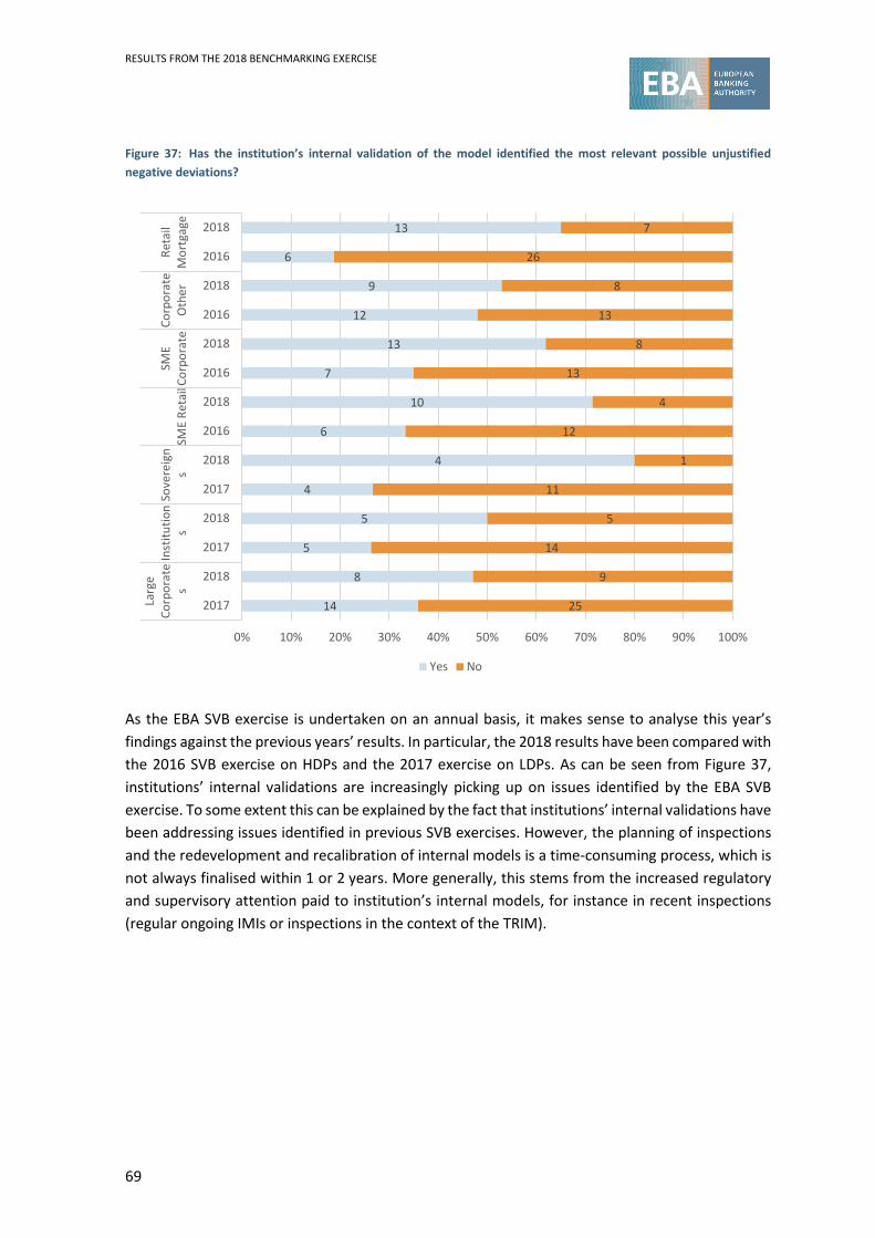
RESULTS FROM THE 2018 BENCHMARKING EXERCISE
69
Figure 37: Has the institution’s internal validation of the model identified the most relevant possible unjustified negative deviations?
As the EBA SVB exercise is undertaken on an annual basis, it makes sense to analyse this year’s findings against the previous years’ results. In particular, the 2018 results have been compared with the 2016 SVB exercise on HDPs and the 2017 exercise on LDPs. As can be seen from Figure 37, institutions’ internal validations are increasingly picking up on issues identified by the EBA SVB exercise. To some extent this can be explained by the fact that institutions’ internal validations have been addressing issues identified in previous SVB exercises. However, the planning of inspections and the redevelopment and recalibration of internal models is a time-consuming process, which is not always finalised within 1 or 2 years. More generally, this stems from the increased regulatory and supervisory attention paid to institution’s internal models, for instance in recent inspections (regular ongoing IMIs or inspections in the context of the TRIM).
14
8
5
5
4
4
6
10
7
13
12
9
6
13
25
9
14
5
11
1
12
4
13
8
13
8
26
7
0% 10% 20% 30% 40% 50% 60% 70% 80% 90% 100%
2017
2018
2017
2018
2017
2018
2016
2018
2016
2018
2016
2018
2016
2018
Larg
eCo
rpor
ate
sIn
stitu
tion
sSo
vere
ign
sSM
E Re
tail
SME
Corp
orat
eCo
rpor
ate
Oth
erRe
tail
Mor
tgag
e
Yes No
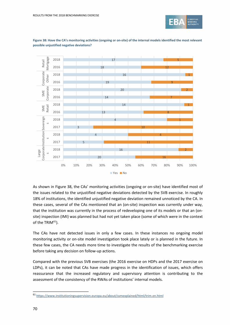
RESULTS FROM THE 2018 BENCHMARKING EXERCISE
70
Figure 38: Have the CA’s monitoring activities (ongoing or on-site) of the internal models identified the most relevant possible unjustified negative deviations?
As shown in Figure 38, the CAs’ monitoring activities (ongoing or on-site) have identified most of the issues related to the unjustified negative deviations detected by the SVB exercise. In roughly 18% of institutions, the identified unjustified negative deviation remained unnoticed by the CA. In these cases, several of the CAs mentioned that an (on-site) inspection was currently under way, that the institution was currently in the process of redeveloping one of its models or that an (on-site) inspection (IMI) was planned but had not yet taken place (some of which were in the context of the TRIM61).
The CAs have not detected issues in only a few cases. In these instances no ongoing model monitoring activity or on-site model investigation took place lately or is planned in the future. In these few cases, the CA needs more time to investigate the results of the benchmarking exercise before taking any decision on follow-up actions.
Compared with the previous SVB exercises (the 2016 exercise on HDPs and the 2017 exercise on LDPs), it can be noted that CAs have made progress in the identification of issues, which offers reassurance that the increased regulatory and supervisory attention is contributing to the assessment of the consistency of the RWAs of institutions’ internal models.
61 https://www.institutioningsupervision.europa.eu/about/ssmexplained/html/trim.en.html
20
16
5
4
3
4
13
14
14
20
19
16
18
17
16
2
11
4
10
1
8
1
7
2
9
1
12
5
0% 10% 20% 30% 40% 50% 60% 70% 80% 90% 100%
2017
2018
2017
2018
2017
2018
2016
2018
2016
2018
2016
2018
2016
2018
Larg
eCo
rpor
ate
sIn
stitu
tion
sSo
vere
ign
sSM
ERe
tail
SME
Corp
orat
eCo
rpor
ate
Oth
erRe
tail
Mor
tgag
e
Yes No

RESULTS FROM THE 2018 BENCHMARKING EXERCISE
71
The questionnaire further enquired as to whether or not any actions are planned by the CA following the SVB results. In more than 52% of the 105 institutions for which the CA submitted the questionnaire, no unjustified negative deviations have been identified, so these cases have not been considered (these are left out in Figure 39). In the majority of cases (66%), where unjustified negative deviations were identified by the SVB exercise, the CAs were already aware of the situation and action is either planned or has taken place already. However, for 17 institutions, the unjustified negative deviations identified by the SVB exercise will lead to further action by the CA. This proves the usefulness of the SVB exercise in identifying undue RWA variability as a driver of model improvement. For 2 out of the 17 institutions, the CA will act in by imposing a capital add-on under Pillar 2.
Figure 39: Are any actions planned by the CA following the SVB results?
3.2 Results of the interviews
The EBA conducted interviews with the 11 institutions for which a significant number of negative deviations had been spotted. The interview teams were mainly composed of representatives of the CAs, members of the EBA Sub-group on Supervisory Benchmarking and EBA staff. The following findings from the interviews help to explain the negative deviations:
• LDPs: the main challenge is to overcome data scarcity, and many issues directly come from the use of approaches to overcome this lack of data. Some institutions use extrapolation techniques to obtain a representative dataset
with a mix of bad and good years (most of the time this extrapolation is performed
17
55
16
16 1
Yes
No, there are no unjustified underestimations
No, the unjustified underestimations were already known by the CA and there is an internal modelinvestigation planned/currently taking placeNo, the unjustified underestimations were already known by the bank (and/or CA) and the bank iscurrently working on the remediation (e.g. re-calibration following model validation)No, the unjustified underestimations were already known and a (material) model change tookplace after the reference date

RESULTS FROM THE 2018 BENCHMARKING EXERCISE
72
at portfolio level), but it is difficult to prove the representativeness of these additional data. The quantification of the MoC is not always clear.
Some institutions use calibration techniques at portfolio level, but it is difficult to prove the representativeness of past data at this level (e.g. some institutions experience massive changes to their portfolio, and it is therefore not clear to what extent the fluctuation of the default rates are due to systemic fluctuation or portfolio composition). The quantification of the MoC is also not always clear.
In cases where the modelling is carried out via a pooling network, additional difficulties may arise, such as the consistent application of the rating methodology between the different members. In cases where the model builds on external ratings, the mapping between the internal and the external rating scale may be subject to different assumptions made during the development of the model that are not always justified.
Given the lack of default observations, any backtesting is challenging. In some cases the performance of the model itself cannot be assessed with certainty.
• HDPs: Apart from general data quality issues, common reasons for negative deviation are: a. No check of the homogeneity at the grade level (when the quantification is done
at the grade and pool level). b. No clear MoC quantification, in particular for the MoC category C62, although most
of the time there is an ‘implicit MoC’ following conservative assumptions made during the model development.
c. No treatment of incomplete workouts (in particular for residential mortgages). d. Sensitivity to the definitions used for the SVB exercise (parameters are exposure-
weighted and not obligor-weighted). • General data quality: some of the deviations are explained by an incorrect mapping of the
counterparties (C 101 template) (but no better identifier than the Legal Entity Identifier (LEI) code could be found), different reporting conventions (for instance for the substitution approach), different definitions of the data points collected (in particular for the loss rate) and general mistakes due to a non-implementation of data quality checks or a lack of resources allocated to this legally binding exercise.
In general, the interviews with the institutions were helpful for the EBA, the CAs and the institutions themselves. They clarified the practices within the institution and provided a better understanding of the institution’s risk assessment as compared with its peers.
3.3 Results of the qualitative survey
In order to explore the impact of different treatments of guarantees and derivatives on the exposure classes in the benchmarking exercise, the EBA conducted a survey with the institutions 62 This concept of MoC category C to account for statistical error is introduced in the GLs on PD and LGD estimation and the treatment of defaulted exposures (https://www.eba.europa.eu/documents/10180/2033363/Guidelines+on+PD+and+LGD+estimation+%28EBA-GL-2017-16%29.pdf/6b062012-45d6-4655-af04-801d26493ed0 ) which apply from 1 January 2021.
RESULTS FROM THE 2018 BENCHMARKING EXERCISE
73
that participated in the 2018 exercise. In this survey, institutions were asked to provide information on the treatments of guarantees and derivatives on the top-level non-defaulted SVB exposure classes: corporates non-SME (separately for AIRB and FIRB) and mortgages (under AIRB). Participation in the survey was voluntary and a total of 94 institutions submitted answers.
The objective of this survey was to gain an overview of the current practices on how guarantees and derivatives are taken into account for the purpose of RWA calculation and, in particular, whether SVB parameters are biased as a result of the incorporation of guarantees and/or derivatives into RW calculation, based on different methods. Three broad methodologies can be isolated that are currently used in the own fund computations to take unfunded credit protection (UFCP) into account:
1. RW substitution, where UFCP is taken into account by substituting the RW of the initial obligor by the RW of the protection provider and applying it to the covered portion of the exposure value. The exposure should be reported as if it were a direct exposure to the guarantor, meaning that it is reported under the exposure class of the guarantor and not that of the obligor.
2. Risk parameters (PD and/or LGD) substitution, where the risk parameter(s) of the guarantor is (are) used instead of the risk parameter of the obligor. Under this approach, there should be a change in exposure class for the reporting under the ITS, meaning that the exposure is reported under the exposure class of the guarantor.
3. Risk parameters (PD and/or LGD) adjustment, where the UFCP is directly taken into account in the model, for instance as a risk driver. Under this approach, there should not be any change in SVB exposure class for reporting in the ITS.
Figure 40 shows that the majority of institutions take guarantees or derivatives into account for the purpose of RWA calculation in the three SVB exposure classes covered in the survey. Note that institutions were instructed to indicate ‘not responded’ if they do not have exposures in the considered SVB portfolio. For mortgage exposures, half of the institutions take guarantees and/or derivatives into account into RWA calculations, whereas for corporate non-SME exposures, 80% of institutions take guarantees into account and 60% take derivatives into account for the purpose of RWA calculation. Some institutions provided reasons for indicating ‘no’. Some mentioned that they do not use guarantees or derivatives in the exposures of the IRB approach models (meaning that they probably have guarantees and derivatives but do not consider them because, for example, they are ineligible). Others mention that the guarantees and/or derivatives are only used in the segmentation of the LGD models and not in the actual estimation of the LGD.

RESULTS FROM THE 2018 BENCHMARKING EXERCISE
74
Figure 40: Institutions taking guarantees or derivatives into account for the purpose of RWA calculation
Some institutions commented on the nature of the guarantees and derivatives taken into account:
a) Based on the comments, there seems to be a limited number of both individual guarantees within corporates-groups and trade guarantees. Derivatives were not mentioned to be used for CRM purposes.
b) Some mention that guarantees are only taken into account if the guarantor is an institution or a government, in which case the institution mentions that only a few exposures in the portfolio are secured by such guarantees.
c) Some institutions mention that the guarantees are guarantees from private individuals, corporate groups, sovereigns or professional guarantees. They mention that the number of exposures covered by guarantees is limited.
Institutions were also asked to indicate the share of the SVB exposure class for which they take guarantees and/or derivatives into account. Overall, the materiality of guarantees and/or derivatives in RWA calculation seems to be limited, in the sense that the share of the portfolios that are covered is usually in the range of 1% to 5%, with a few exceptions of up to 10%. Figure 41 shows the distribution in the different methodologies to take UFCP into account, organised by the type of the guarantor (SA, FIRB or AIRB guarantor)63.
63 It should be mentioned that in this figure and in the following charts, the responses are summarised on an institution basis, i.e. whenever an institution makes use of a technique it is counted as a 1, and 0 otherwise, in contrast to the question included the survey, in which respondents were asked for the share of the EAD in the respective portfolio, for which they apply the considered technique. As a result of data quality reasons, it was not possible to summarise the shares of the portfolios treated under each technique. In the charts where the results are presented across the different SVB exposure classes, the simple sum is taken, meaning that an institution that takes guarantees and/or derivatives into account in the three SVB exposures classes, is counted three times. In addition, only the responses of institutions that responded ‘yes’ to the first question (i.e. ‘Do you take guarantees or derivatives into account for the purpose of RWA calculation?’) are included.
49
29
35
11
19
35
34
46
24
0% 10% 20% 30% 40% 50% 60% 70% 80% 90% 100%
Corporate non-SME (AIRB)
Corporate non-SME (FIRB)
Mortgages (AIRB)
Yes No Did not respond

RESULTS FROM THE 2018 BENCHMARKING EXERCISE
75
Figure 41: Distribution of methodologies for the treatment of guarantees and derivatives in RWA calculation by type of guarantor
SA guarantors are taken into account mostly via RW substitution, whereas FIRB guarantors are taken into account mostly via PD substitution. AIRB guarantors are taken into account via different methods, with LGD adjustments only (i.e. by using historical cash flows from guarantees as shown in Figure 46) being the most common method, and PD and LGD substitution, and PD substitution only being the second and third most common methods. Figure 42 to Figure 44 provide the same information, organised by exposure class. Special attention should be paid to the (low) numbers of observations. In particular, the number of FIRB guarantors is negligible for exposures treated under the AIRB approach and the number of AIRB guarantors is particularly low for exposures treated under the FIRB approach.
0
1
1
11
2
29
1
0
5
0
16
17
0
0
3
0
1
18
47
5
5
2
0
2
0% 10% 20% 30% 40% 50% 60% 70% 80% 90% 100%
SA guarantors
FIRB guarantors
AIRB guarantors
PD adjustment only LGD adjustment only PD and LGD adjustment
PD substitution only LGD substitution only PD and LGD substitution
RW substitution Other

RESULTS FROM THE 2018 BENCHMARKING EXERCISE
76
Figure 42: Distribution of methodologies for the treatment of guarantees and derivatives in RWA calculation by type of guarantor (corporate non-SME exposures in the AIRB)
Figure 43: Distribution of methodologies for the treatment of guarantees and derivatives in RWA calculation by type of guarantor (corporate non-SME exposures in the FIRB)
0
0
1
6
1
14
1
0
3
0
1
11
0
0
2
0
0
14
20
0
3
0
0
1
0% 20% 40% 60% 80% 100%
SA
FIRB
AIRBPD adjustment only
LGD adjustment only
PD and LGD adjustment
PD substitution only
LGD substitution only
PD and LGD substitution
RW substitution
Other
0
1
0
0
0
0
0
0
0
0
15
1
0
0
1
0
1
0
18
5
0
2
0
0
0% 20% 40% 60% 80% 100%
SA
FIRB
AIRBPD adjustment only
LGD adjustment only
PD and LGD adjustment
PD substitution only
LGD substitution only
PD and LGD substitution
RW substitution
Other

RESULTS FROM THE 2018 BENCHMARKING EXERCISE
77
Figure 44: Distribution of methodologies for the treatment of guarantees and derivatives in RWA calculation by type of guarantor (mortgages)
Figure 45 and Figure 46 provide further insight into how institutions perform PD and LGD adjustments. Note that the sample size in these charts is relatively small (16 institutions for PD adjustments and 43 for LGD adjustments), therefore the conclusions should be interpreted with caution. For PD adjustments, the most common method is to use the information of the existence of the guarantee in risk differentiation. However, five institutions indicated that they use other techniques. One institution mentioned that the technique used depends on the model: in some cases, the rating grade is adjusted via an override, in other cases the guarantor is a (hard or soft) input factor of in the model. As shown in Figure 46, LGD adjustments are performed mostly on the basis of historical cash flows from guarantees. Figure 45: How are PD adjustments performed?
0
0
0
5
1
15
0
0
2
0
0
5
0
0
0
0
0
4
9
0
2
0
0
1
0% 20% 40% 60% 80% 100%
SA
FIRB
AIRBPD adjustment only
LGD adjustment only
PD and LGD adjustment
PD substitution only
LGD substitution only
PD and LGD substitution
RW substitution
Other
7
5
3
1
by using the information of the existence (or level, or ratinggrade of the guarantor, etc.) of the guarantee in riskdifferentiation
other
by adjusting the rating grade via an override
by scope of application

RESULTS FROM THE 2018 BENCHMARKING EXERCISE
78
Figure 46: How are LGD adjustments performed?
Institutions were also asked whether they change the RW function (i.e. Article 153 versus Article 154 of the CRR). The CRR is silent on this aspect and does not mention that institutions should change the RW function if they use UFCP64. Note that this aspect is a prudential aspect, which is different from the reporting aspect mentioned in the beginning of this section, whereby institutions should change the exposure class for the reporting under the ITS, in cases in which they apply RW, PD or LGD substitution. Figure 47 summarises these responses and it can be seen that the majority of the institutions change the RW function but several institutions keep the exposure under the original exposure class, even though it is (partly) secured by a guarantee or derivative. As such, these guaranteed exposures are part of the computed benchmarks and are expected to drive the level of the benchmark down, and therefore complicate the detection of outliers for the purpose of the SVB exercise.
64 According to EBA Q&A 2013_415, the change in risk weight function is not required, as neither Article 161(3) nor 236(1) of the CRR require the use of a different risk weight function or asset value correlation. The CRM report seems to actually suggest that the risk weight function should not be changed and ‘the risk weight function to be used for the covered portion of the exposure by the UFCP is the same one used for the uncovered part of the exposure’ in paragraph 44.
284
12
8
LGD estimation based on historical cash flows fromguarantees
LGD estimation based on hypothetical cash flowsfrom the guarantee
by scope of application
by adjusting the facility grade via an override
other

RESULTS FROM THE 2018 BENCHMARKING EXERCISE
79
Figure 47: If using PD and/or LGD substitution, is the RW function changed?
The final question is the extent to which benchmarking parameters are biased as a result of the incorporation of guarantees. To answer this question, the responses in this survey have been analysed in relation to the reported PD, LGD and RW estimates (under the regular SVB reporting) (with and without guarantees and/or derivatives in the estimation) and to the observed variability in the respective SVB exposure classes (the interquartile range). Ex-ante, considering the low materiality of the use of UFCP, the contribution of different practices to the observed variability and the possible bias to the benchmarks (mean PD, LGD and RW) is likely to be limited. Nevertheless, there is still a possibility that the use of UFCP adversely affects outlier detection. Based on the data reported, it is not possible to find evidence that the use of guarantees and/or derivatives significantly affects the level of PD, LGD and/or RW estimates across SVB exposure classes. These conclusions are based on the figures reported in Figure 48 to Figure 50. The orange bars in Figure 48 to Figure 50 indicate interquartile ranges (i.e. first and third quartile) that have been computed on those institutions that responded ‘yes’ or ‘no’ to the first question in the survey, i.e. whether they take guarantees and/or derivatives into account in the RWA calculation. The ‘yes’ (marked as a red triangle) corresponds to the average PD, LGD and RW of the institutions that indicated that they take guarantees and/or derivatives into account in the RWA calculation, whereas the ‘no’ (marked as a black square) corresponds to the average PD, LGD and RW of those that indicated no. A priori, one would expect that institutions which do take guarantees and/or derivatives into account, have a lower PD, LGD and RW than the other institutions. However, this finding cannot be confirmed based on the responses received from the survey. For corporate non-SME exposures,
42
21
3
Yes No Other

RESULTS FROM THE 2018 BENCHMARKING EXERCISE
80
the average PD of those institutions making use of derivatives and/or guarantees is within the interquartile range of PD estimates (see Figure 48), whereas the average PD estimate is higher (and above the interquartile range) for mortgage exposures, which is contrary to our null hypothesis. However, one potential explanation could be that institutions specifically require a guarantor or hedge (derivative) in cases in which the exposure is particularly risky. However, the number of observations is sometimes quite low, as shown in Table 10, in particular for corporate non-SME exposures. Table 10: Number of observations (institutions), by SVB exposure class, reporting yes or no, on whether they use guarantees and/or derivatives in RWA calculations
Corporate non-SME (AIRB) Corporate non-SME (FIRB) Mortgages (AIRB) No 2 8 26 Yes 41 26 32
Figure 48: Effect of the use of guarantees and/or derivatives on the PD estimate
For the effects on the LGD estimates and the RWs (see Figure 49 and Figure 50), the responses to the survey also do not provide conclusive evidence that the use of guarantees and/or derivatives in the RWA calculation would bias benchmarking parameters. In particular, it can be seen that the average LGD and RW estimates of the ‘Yes/No’ respondents are within the interquartile ranges, except for the LGD estimates of corporate non-SME exposures (AIRB), where institutions that do not make use of guarantees and/or derivatives appear to experience an LGD estimate which is lower than most others (i.e. it is below the interquartile range). However, this is contrary to the null hypothesis.
0%
1%
1%
2%
2%
3%
3%
4%
4%
5%
Corporate non SME (AIRB) Corporate non SME (FIRB) Mortgages (AIRB)
Yes No

RESULTS FROM THE 2018 BENCHMARKING EXERCISE
81
Figure 49: Effect of the use of guarantees and/or derivatives on the LGD estimate
Figure 50: Effect of the use of guarantees and/or derivatives on the RW
Overall, it should be kept in mind that the small sample size may be the reason that it is not possible to find a significant impact. Furthermore, it should be mentioned that it is still possible that outlier detection is adversely affected by the use of guarantees and/or derivatives.
0%
5%
10%
15%
20%
25%
30%
35%
40%
Corporate non SME (AIRB) Mortgages (AIRB)
Yes No
0%
20%
40%
60%
80%
100%
120%
Corporate non SME (AIRB) Corporate non SME (FIRB) Mortgages (AIRB)
Yes No

RESULTS FROM THE 2018 BENCHMARKING EXERCISE
82
Conclusion
This report presents the results of the SVB exercise for HDPs and LDPs, conducted pursuant to Article 78 of the CRD and the related technical standards on the internal approaches for credit risk. In particular, the SVB exposure classes considered in this year’s exercise are: large corporates, sovereigns and institutions (LDPs) and residential mortgages, SME retail, SME corporate and corporate-other portfolios (HDPs).
The analysis is based on data reported at the highest level of consolidation. At the end of December 2017, 117 institutions had their credit risk internal models approved. A total of 114 institutions, across 17 EU countries, contributed to the SVB exercise, submitting at least one counterparty and/or portfolio 65 . Qualitative information on specific aspects has been collected through (i) individual assessments by CAs of all institutions, (ii) interviews with a sample of 11 institutions and (iii) a qualitative survey on the use of the substitution effect across all institutions.
First, the EBA took a top-down approach to quantifying the proportion of variability that can be explained by some key drivers. Differences in the share of the defaulted exposures and the portfolio mix effect explain around 50% of GC variability observed in the data. The remaining 50% may be due to differences in institution-specific factors, such as risk management practices. This confirms previous findings that RWA variability can be explained, to a large extent, by looking at some measurable features of institutions’ exposures.
An in-depth analysis has been performed on the LDPs, by means of a common counterparties analysis. Most of the interquartile ranges of the deviations resulting from benchmark substitution are below 10%. These interquartile differences are greater under the AIRB approach than under the FIRB approach for large corporate exposures and sovereigns. In the AIRB approach, the interquartile difference is greatest for exposures to large corporates. Finally, there is a strong non-linearity effect, in the sense that the variability in the different risk parameters is compensating (the total deviation is well below the sum of the deviation of each risk parameter): in short, low PD estimates are generally associated with high LGD estimates, and vice versa.
For the HDPs, the outturns analysis provided further insight into the variability in risk parameters across institutions. Overall, the RWA analysis does not reveal a material negative deviation of the estimated level of risk compared with the observed level of risk for the vast majority of EU institutions. With regard to the ratio of the default rate to the PD estimate, the results show that the great majority of institutions have conservative estimates, in particular for the default rate for the past year. This analysis corroborates the hypothesis that the portfolio mix and the regulatory approach are key drivers of variability both for the risk parameters and the RWAs. With regard to the ratio of the loss rate and the LGD estimate, the results show that for at least 75% of the
65 This is because three institutions do not have exposures in scope of the SVB exercise.

RESULTS FROM THE 2018 BENCHMARKING EXERCISE
83
institutions, the portfolio estimated LGD is higher than the loss rate observed in the past year or over the past 5 years, which again indicates conservative behaviour on the part of the institutions66.
A comparison of the results of this year’s SVB exercise with the previous ones (the 2016 exercise on HDPs and the 2017 exercise on LDPs) shows that there is stability in the reported parameters, such as RW, PD and LGD, with the exception of the PD for large corporates under the FIRB and AIRB approaches, for which an increase in the PD has been observed. For the LDPs, the variability in estimates was stable over the two exercises. For the HDPs, in general, both default and loss rates have decreased more than PD and LGD estimates in recent years. This is likely to reflect a general improvement in economic conditions.
CAs provided individual assessments on the quality of the benchmarked models for each institution. The focus of the assessments by the CAs has been on the RWs (of non-defaulted exposures) (note that FIRB institutions assign a zero RW to defaulted exposures). For the majority of the institutions, the RW deviations from the EU benchmarks were deemed to be justified by the CAs. The highest share of unjustified negative deviations from the benchmarks can be observed for exposures to corporates. It should be kept in mind, however, that this means that these are outlier values resulting from modelling, which are treated as an indication of significant differences in own funds requirements, and that therefore a specific assessment by the CA is needed.
Problems with the calibration of the risk parameters is mentioned as the main reason for these unjustified underestimations, but there are other concerns related to, inter alia, data quality, differences in definitions used, the design of the ranking model, the absence of models for LGD-in-default estimates and ELBE, and deficiencies in the framework for the review of estimates. It is reassuring that most aspects are being addressed in the EBA GLs on PD and LGD estimation.
The CAs’ assessments also revealed that the majority of institutions’ internal validations identified the unjustified negative deviation identified in the SVB exercise. It is also reassuring that the CAs’ monitoring activities (ongoing or on-site) have identified most of the issues related to the unjustified negative deviations detected by the SVB exercise. For a small sample of institutions, the unjustified negative deviations identified by the SVB exercise will lead to further action by the CA. This proves the usefulness of the SVB exercise in identifying undue RWA variability as a driver of model improvement.
In comparison with previous exercises, institutions’ internal validations as well as the CAs’ monitoring activities (ongoing or on-site) are increasingly picking up on issues identified by the EBA SVB exercise. This is reassuring and indicates that the increased regulatory and supervisory attention paid to internal models is contributing to the consistency of the RWA of internal models.
The EBA has, together with the CAs, conducted interviews with the 11 institutions for which the highest number of outlier observations were spotted. For LDPs, many of the identified outlier observations relate to methodological problems with techniques to overcome data scarcity, i.e.
66 However, since the loss rate in the analysis is not purely observed, but calculated using the institution’s estimate, these results should be interpreted with caution and complemented by a case-by-case analysis.

RESULTS FROM THE 2018 BENCHMARKING EXERCISE
84
extrapolation techniques, problems with backtesting, or difficulties with calibration techniques at portfolio level. For HDPs, the interviews highlighted that, in some cases, the institution had performed its risk quantification at the grade or pool level without checking homogeneity at the grade level. In other cases, there was no treatment of incomplete workout scenarios. Finally, some of the outlier observations were due to sensitivity to the definitions used for the SVB exercise (exposure-weighted versus obligor-weighted parameters). Furthermore, there seemed to be several misunderstandings with respect to the revised concept of MoC, as introduced in the EBA Guidelines on PD and LGD. In general, the interviews were useful because they allowed a number of points to be clarified.
The results of the survey on the treatment of guarantees and derivatives show that the majority of institutions take guarantees or derivatives into account for the purpose of the RWA calculation in the exposure classes covered in the survey (corporate non-SME under the FIRB and AIRB approaches, as well as mortgages). However, the materiality of guarantees and/or derivatives in the RWA calculation seems to be limited, in the sense that the share of the exposures which are covered are usually in the range of 1 to 5%. SA guarantors are taken into account mostly via RW substitution, whereas FIRB guarantors are taken into account mostly via PD substitution. AIRB guarantors are taken into account via a range of different methods. The results do not show evidence that benchmarking parameters are systematically biased as a result of the use of guarantees or derivatives, which is a positive message. Nevertheless, it is still possible that the outlier detection is adversely affected because of the use of guarantees and/or derivatives.
Future work
The EBA will continue to provide a regular EU overview of existing RWA variability and drivers of differences on the basis of the SVB framework. The SVB framework has been implemented as an annual supervisory tool, and will continue to support comparison among peer institutions and help to summarise the results of the CAs’ assessments of the quality of the internal approaches in use, and of the measures currently under consideration for improvement by both institutions and supervisors. For future exercises, and with the benefit of a stable sample of institutions and clearer reporting definitions, more emphasis on comparisons across time will help to gain additional insight as to whether convergence in modelling practices is taking place as a result of the EBA review of internal models.
The results of the SVB exercises are taken into account in the work the EBA is conducting in parallel on the validation of internal models, which contributes to harmonising supervisory and institutions’ practices and enhances consistency. This work includes using existing EBA Guidelines, where appropriate, to enhance convergence in the computation of RWAs, and to improve Pillar 3 disclosures, as well as in the validation and ongoing monitoring of internal models. In 2016, the EBA set out a roadmap specifying the general principles and timelines for the implementation of the regulatory review of the internal models for credit risk. Among several measures, it introduced changes aimed at harmonising definitions and supervisory practices in the definition of default, the

RESULTS FROM THE 2018 BENCHMARKING EXERCISE
85
estimation of risk parameters and treatment of defaulted assets, CRM techniques and disclosure in four phases67.
It was, however, noticed that the main issues identified in this SVB exercise are not materially different from those identified in the previous exercises, i.e. many institutions and/or CAs were already aware of the issues, and an IMI is pending or currently taking place, or the institution is currently redeveloping and/or recalibrating its model, or a (material) model change has already taken place.
In addition, most of the issues identified by the CA as reasons for unjustified negative deviations are being addressed, with further guidance published in the GLs on PD and LGD. However, given that institutions have until the end of 2020 to implement the changes introduced by the GLs in PD, LGD and defaulted assets, there are still 2 years left for the institutions to effect these.
There are, however, two main areas where further work would be justified. First, there is still room for improvement in the current ITS on SVB to adequately capture the use of the different CRM techniques. This is important because ideally the outlier rule should be able to correctly detect all relevant outliers. This would mean in particular, minimising the cases where the outlier rule is not able to detect cases where the internal model outcome is an outlier as compared with its peers. This applies to the objective of minimising type II errors, i.e. accepting a false null hypothesis. In addition, we know from the CAs’ assessments that several institutions for which one of their portfolios has been flagged as an outlier, a high degree of collateralisation explains the negative deviation from the benchmark. As such, the deviation has been deemed to be justified by the CA. However, the outlier rule should also minimise the occurrence of false outlier observations, i.e. it should minimise the occurrence of type I errors (rejecting a true null hypothesis). It therefore seems appropriate to amend the SVB ITS in order to adequately capture the use of different CRM techniques. Furthermore, the EBA is currently drafting GLs on CRM techniques, which should ensure a greater consistency in the use of these techniques.
A second area where further work should be carried out is the comparison of RWA (or GC) with the hypothetical RWA (or GC) that would apply if the exposure were to be treated under the SA. Indeed, the scope of the benchmarking exercise is to analyse drivers of unjustified variability in internal models, but given that many of the known drivers of variability have already been addressed in the EBA project on internal model repair, it makes sense to benchmark the variability stemming from the internal model outcomes with those that would be applicable if the exposure were treated under the SA. Data on this aspect, i.e. the requirements for credit risk exposures that would apply if using the SA, will be collected through the 2019 ITS, on a mandatory basis for HDPs and on a voluntary basis for LDPs. As such, the comparison of the variability in internal models with the variability in the SA will provide an additional benchmark to assess whether the current levels of variability are justified or not.
67 EBA model validation. https://www.eba.europa.eu/regulation-and-policy/model-validation

RESULTS FROM THE 2018 BENCHMARKING EXERCISE
86
Data quality constraints from some institutions also deserve attention from CAs, given the possible data limitations and the need for improvements in their internal general data collection systems, IT infrastructures and database level. Moreover, the ITS on SVB needs further development to allow a common understanding to be gained of the reporting requirements. In addition, more guidance might be provided to the CAs on the EBA benchmark and the assessment of the SVB results.

RESULTS FROM THE 2018 BENCHMARKING EXERCISE
87
Annex 1: List of participating institutions
The institutions within the scope of the SVB exercise are those that, at 31 December 2017, had approval for the use of the credit risk internal models. The EBA collects this information through the CAs at the beginning of each year and publishes it on the EBA website soon after the approval of the board of supervisors 68 . For the 2018 SVB exercise, which has the reference date of 31 December 2017, this collection was done in January 2018 and the list was published at the beginning of March 2018. The list, reproduced in Table 11, is purely informative.
A disclaimer: if an institution has a credit risk internal model approved within that date but is not on the list, they still have to report, and they are kindly invited to inform their CAs and ask for the information to be amended.
Table 11: List of institutions participating in this exercise
Institution name Country Submits
credit risk?
BAWAG Group AG Austria Yes Raiffeisen Bank International AG Austria Yes Erste Group Bank AG Austria Yes Volkskredit Verwaltungsgenossenschaft reg.Gen.m.b.H. Austria Yes KBC Group NV Belgium Yes Belfius Banque SA Belgium Yes Investar Belgium Yes Dexia NV Belgium Yes AXA Bank Europe SA Belgium Yes Crelan Belgium Yes Euroclear SA Belgium Yes Jyske Bank A/S Denmark Yes Nykredit Realkredit A/S Denmark Yes Danske Bank A/S Denmark Yes Sydinstitution A/S Denmark Yes Lån og Spar Bank A/S Denmark Yes DLR Kredit A/S Denmark Yes OP-Pohjola Group Finland Yes Ålandsinstitutionen Plc Finland Yes Aktia Bank Finland Yes Groupe BPCE France Yes Groupe Credit Agricole France Yes Société Générale SA France Yes
68 https://www.eba.europa.eu/documents/10180/15926/EBA+list+of+institutions+for+the+purpose+of+supervisory+benchmarking.pdf/95c17f4b-b8dd-4bec-964c-36478a34b92f

RESULTS FROM THE 2018 BENCHMARKING EXERCISE
88
Institution name Country Submits
credit risk?
BNP Paribas SA France Yes SFIL (Société de Financement Local) France Yes RCI banque (Renault Crédit Industriel) France Yes Crédit Mutuel Group France Yes BANQUE ACCORD France Yes CARREFOUR BANQUE France Yes GOLDMAN SACHS PARIS INC ET CIE France Yes Erwerbsgesellschaft der S-Finanzgruppe mbH & Co. KG Germany Yes Deutsche Zentral-Genossenschaftsinstitution AG Germany Yes Deutsche Bank AG Germany Yes Commerzinstitution AG Germany Yes Landesinstitution Baden-Württemberg Germany Yes Landesinstitution Hessen-Thüringen Girozentrale Germany Yes NORD/LB Norddeutsche Landesinstitution Girozentrale Germany Yes DekaBank Deutsche Girozentrale Germany Yes Deutsche Apotheker- und Ärzteinstitution eG Germany Yes Münchener Hypothekeninstitution eG Germany Yes Deutsche Pfandbriefinstitution AG Germany Yes Aareal Bank AG Germany Yes HSH Beteiligungs Management GmbH Germany Yes Bayerische Landesinstitution Germany Yes LBS Bayerische Landesbausparkasse Germany Yes Landesinstitution Saar Germany Yes Oldenburgische Landesinstitution AG Germany Yes Süd-West-Kreditinstitution Finanzierung GmbH Germany Yes ALTE LEIPZIGER Bauspar AG Germany Yes KfW Beteiligungsholding Germany Yes Wüstenrot Bausparkasse AG Germany Yes TOYOTA Kreditinstitution GmbH Germany Yes SVBW Bank GmbH Germany Yes Degussa Bank Germany Yes Deutsche Bausparkasse Badenia AG Germany Yes Alpha Bank AE Greece No National Bank of Greece SA Greece Yes Euroinstitution Greece Yes Group of Magyar Takarékszövetkezeti Bank Zrt. Hungary Yes AIB Group plc Ireland Yes Permanent TSB Group Holdings Plc Ireland Yes Bank of Ireland Group plc Ireland Yes Intesa Sanpaolo SpA Italy Yes Banco BPM Italy Yes UniCredit SpA Italy Yes BPER Banca SpA Italy Yes Credito Emiliano Holding SpA Italy Yes Unione di Banche Italiane SCpA Italy Yes
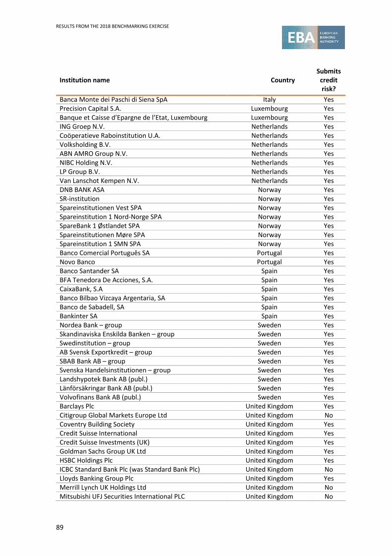
RESULTS FROM THE 2018 BENCHMARKING EXERCISE
89
Institution name Country Submits
credit risk?
Banca Monte dei Paschi di Siena SpA Italy Yes Precision Capital S.A. Luxembourg Yes Banque et Caisse d’Epargne de l’Etat, Luxembourg Luxembourg Yes ING Groep N.V. Netherlands Yes Coöperatieve Raboinstitution U.A. Netherlands Yes Volksholding B.V. Netherlands Yes ABN AMRO Group N.V. Netherlands Yes NIBC Holding N.V. Netherlands Yes LP Group B.V. Netherlands Yes Van Lanschot Kempen N.V. Netherlands Yes DNB BANK ASA Norway Yes SR-institution Norway Yes Spareinstitutionen Vest SPA Norway Yes Spareinstitution 1 Nord-Norge SPA Norway Yes SpareBank 1 Østlandet SPA Norway Yes Spareinstitutionen Møre SPA Norway Yes Spareinstitution 1 SMN SPA Norway Yes Banco Comercial Português SA Portugal Yes Novo Banco Portugal Yes Banco Santander SA Spain Yes BFA Tenedora De Acciones, S.A. Spain Yes CaixaBank, S.A Spain Yes Banco Bilbao Vizcaya Argentaria, SA Spain Yes Banco de Sabadell, SA Spain Yes Bankinter SA Spain Yes Nordea Bank – group Sweden Yes Skandinaviska Enskilda Banken – group Sweden Yes Swedinstitution – group Sweden Yes AB Svensk Exportkredit – group Sweden Yes SBAB Bank AB – group Sweden Yes Svenska Handelsinstitutionen – group Sweden Yes Landshypotek Bank AB (publ.) Sweden Yes Länförsäkringar Bank AB (publ.) Sweden Yes Volvofinans Bank AB (publ.) Sweden Yes Barclays Plc United Kingdom Yes Citigroup Global Markets Europe Ltd United Kingdom No Coventry Building Society United Kingdom Yes Credit Suisse International United Kingdom Yes Credit Suisse Investments (UK) United Kingdom Yes Goldman Sachs Group UK Ltd United Kingdom Yes HSBC Holdings Plc United Kingdom Yes ICBC Standard Bank Plc (was Standard Bank Plc) United Kingdom No Lloyds Banking Group Plc United Kingdom Yes Merrill Lynch UK Holdings Ltd United Kingdom No Mitsubishi UFJ Securities International PLC United Kingdom No
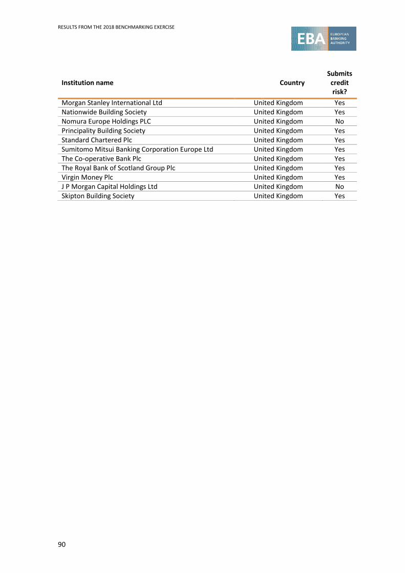
RESULTS FROM THE 2018 BENCHMARKING EXERCISE
90
Institution name Country Submits
credit risk?
Morgan Stanley International Ltd United Kingdom Yes Nationwide Building Society United Kingdom Yes Nomura Europe Holdings PLC United Kingdom No Principality Building Society United Kingdom Yes Standard Chartered Plc United Kingdom Yes Sumitomo Mitsui Banking Corporation Europe Ltd United Kingdom Yes The Co-operative Bank Plc United Kingdom Yes The Royal Bank of Scotland Group Plc United Kingdom Yes Virgin Money Plc United Kingdom Yes J P Morgan Capital Holdings Ltd United Kingdom No Skipton Building Society United Kingdom Yes

RESULTS FROM THE 2018 BENCHMARKING EXERCISE
91
Annex 2: Data quality
The LDP and HDP information constitutes a subset of the SVB exercise related to credit risk, as laid down in the ITS drafted by the EBA, pursuant to Article 78 of Directive 2013/36/EU (CRD IV) from the European Commission. This represents the first official data collection with the full scope for credit risk. Some constraints that emerged during the collection of these data (and that were confirmed during interviews with institutions) can be summarised as follows:
(i) Difficulties in the implementation of the ITS due to its late publication. (ii) Challenges in the mapping of the counterparties, although the LEI seems to be present
in their systems. (iii) Because of the yearly changes to the ITS, not all the institutions are able to implement
automatic extraction of the figures. Different practices have been mentioned during the interviews: a. some of the institutions have implemented automatic checks for the portfolio
breakdown; b. others did the collection manually using Excel files; c. some of the institutions have created a dedicated database for the SVB (the ones
that have COREP databases or risk databases), while others have integrated the SVB templates in the same databases;
(iv) Unavailability of data as a result of incomplete submissions (incomplete submissions for templates, e.g. buckets, breakdowns and data relationships, as well as at overall portfolio level).
(v) Poor data quality and implausible figures (e.g. percentage values multiplied by 100, against existing guidance, due mainly to the merging of figures from different systems or from different entities).

RESULTS FROM THE 2018 BENCHMARKING EXERCISE
92
Annex 3: Data cleansing
From a total of 124 institutions that have had their internal models approved (Annex 1), 117 have credit risk internal models approved by their supervisors. These 117 institutions fall into the scope of the present exercise. However, institutions might not have had exposures, as described in Annex 1 and the information collected under templates C 101.00, C 102.00 and C 103.00, in their balance sheet at the reference date of Q4 2017.
The cut-off date for the extraction of the data for this report was 21 September 2018.
The records with portfolio IDs or counterparty codes not in the list in Annex I were excluded from the analyses throughout in this report. In general, the records with PDs not between 0% and 100% (extremes included) were excluded from the analysis. Incoherent combinations of ‘default status’ and ‘PD’ values were also excluded (example: non-defaulted exposure with PD = 100%).
Template C 101.00
For template C 101.00, where exposures to a predefined list of common counterparties are gathered, only 85 institutions, from 16 different countries, submitted information for at least one counterparty with EAD greater than zero.
For the purpose of ensuring sufficient data quality:
• Records with negative LGD, maturity and RWA have been excluded.
• If an institution submitted the same counterparty ID more than once with a different rating grade (see Q&A 2017_3635), that counterparty ID has been excluded for that institution.
For the purpose of the computation of the benchmarks (median of the values) at counterparty level:
• Only counterparty codes submitted by at least five institutions have been considered.
• All the counterparties that have been classified in default by at least one institution have been excluded (no benchmarks have been computed for them).
• The counterparties of any particular institution have been considered only if the institution has submitted at least 10 counterparties with EAD greater than zero.
• Counterparties with reported LGD greater than 150% or RW% greater than 500% have been excluded.

RESULTS FROM THE 2018 BENCHMARKING EXERCISE
93
Table 12: Sample of institutions, countries and counterparties in the common counterparty analysis (LDPs)
SVB exposure class
Number of institutions
Countries of the institutions
Number of different counterparties reported
Number of counterparties for which the benchmarks have been computed
Countries of the counterparties reported
Institutions sample 67 15 851 668 36 Large corporate sample 76 15 9325 2494 37 Sovereign sample 49 12 378 202 55
Template C 102.00 and C 103.00
With these templates, the total amount and risk parameters of all the SVB exposure classes in the LDPs (C 102.00) and the HDPs (C 103.00) that are under the IRB approach and that are real exposures for the institution were collected. The different portfolios have different features to be able to compare homogenous portfolios between institutions.
For the purpose of ensuring sufficient data quality:
• Records with negative LGD, maturity and RWA were excluded.
For the purpose of the computation of the benchmarks (median of the values) at portfolio level:
• Only the portfolio IDs not related to the rating breakdown were considered (those portfolios have been used to analyse the risk concentration in the tool provided to the CAs).
• Only portfolios submitted by at least five institutions were considered.
• Only those portfolio IDs with at least five obligors were considered. (The portfolio IDs in which the institution has fewer than five obligors have been considered for the quality check, top-down and all the other analysis, but not for the computation of the benchmarks).
• Only portfolio IDs with an EAD > EUR 10 000 were considered. (The portfolio IDs in which the institution has less than EUR 10 000 EAD have been considered for the quality check, top-down and all the other analysis but not for the computation of the benchmarks).

RESULTS FROM THE 2018 BENCHMARKING EXERCISE
94
• Records reported with LGD > 150% or RW% > 500% have been excluded in the computation of the benchmarks.
For template C 102.00, which covers the various portfolios relating to the LDP SVB exposure classes (institutions, large corporates and sovereigns), only 97 out of 117 institutions returned the template.
Table 13: Sample of institutions, countries and counterparties in the portfolio analysis (LDPs) (C 102.00)
SVB exposure class Number of institutions Countries of the institutions
Number of different portfolios reported
Number of portfolios for which the benchmarks have been computed
Sovereigns 51 11 654 43 Institutions 68 15 978 143 Large corporate 91 17 556 147 Large corporate sample 72 15 289 25
For template C 103.00, which covers HDP exposures (corporate-other, residential mortgages, SME retail and SME-corporate), only 108 out of 117 institutions returned the template.
Table 14: Sample of institutions, countries and counterparties in the portfolio analysis (HDPs) (C 103.00)
SVB exposure class Number of institutions Countries of
the institutions
Number of different portfolios reported
Number of portfolios for
which the benchmarks have been computed
Corporate 89 17 10399 307 Mortgages 89 17 4927 420 SME retail 89 17 10471 248 SME corporate 74 16 4743 230
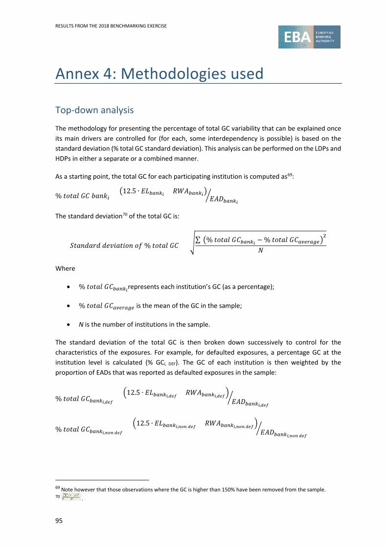
RESULTS FROM THE 2018 BENCHMARKING EXERCISE
95
Annex 4: Methodologies used
Top-down analysis
The methodology for presenting the percentage of total GC variability that can be explained once its main drivers are controlled for (for each, some interdependency is possible) is based on the standard deviation (% total GC standard deviation). This analysis can be performed on the LDPs and HDPs in either a separate or a combined manner.
As a starting point, the total GC for each participating institution is computed as69:
% 𝑡𝑡𝑡𝑡𝑡𝑡𝑡𝑡𝑡𝑡 𝐺𝐺𝐺𝐺 𝑏𝑏𝑡𝑡𝑏𝑏𝑏𝑏𝑖𝑖 = �12.5 ∙ 𝐸𝐸𝐸𝐸𝑏𝑏𝑏𝑏𝑏𝑏𝑏𝑏𝑖𝑖 + 𝑅𝑅𝑅𝑅𝑅𝑅𝑏𝑏𝑏𝑏𝑏𝑏𝑏𝑏𝑖𝑖�𝐸𝐸𝑅𝑅𝐸𝐸𝑏𝑏𝑏𝑏𝑏𝑏𝑏𝑏𝑖𝑖�
The standard deviation70 of the total GC is:
𝑆𝑆𝑡𝑡𝑡𝑡𝑏𝑏𝑆𝑆𝑡𝑡𝑆𝑆𝑆𝑆 𝑆𝑆𝑑𝑑𝑑𝑑𝑑𝑑𝑡𝑡𝑡𝑡𝑑𝑑𝑡𝑡𝑏𝑏 𝑡𝑡𝑜𝑜 % 𝑡𝑡𝑡𝑡𝑡𝑡𝑡𝑡𝑡𝑡 𝐺𝐺𝐺𝐺 = �∑ �% 𝑡𝑡𝑡𝑡𝑡𝑡𝑡𝑡𝑡𝑡 𝐺𝐺𝐺𝐺𝑏𝑏𝑏𝑏𝑏𝑏𝑏𝑏𝑖𝑖 − % 𝑡𝑡𝑡𝑡𝑡𝑡𝑡𝑡𝑡𝑡 𝐺𝐺𝐺𝐺𝑏𝑏𝑎𝑎𝑎𝑎𝑎𝑎𝑏𝑏𝑎𝑎𝑎𝑎�2
𝑁𝑁
Where
• % 𝑡𝑡𝑡𝑡𝑡𝑡𝑡𝑡𝑡𝑡 𝐺𝐺𝐺𝐺𝑏𝑏𝑏𝑏𝑏𝑏𝑏𝑏𝑖𝑖represents each institution’s GC (as a percentage);
• % 𝑡𝑡𝑡𝑡𝑡𝑡𝑡𝑡𝑡𝑡 𝐺𝐺𝐺𝐺𝑏𝑏𝑎𝑎𝑎𝑎𝑎𝑎𝑏𝑏𝑎𝑎𝑎𝑎 is the mean of the GC in the sample;
• N is the number of institutions in the sample.
The standard deviation of the total GC is then broken down successively to control for the characteristics of the exposures. For example, for defaulted exposures, a percentage GC at the institution level is calculated (% GCi, DEF). The GC of each institution is then weighted by the proportion of EADs that was reported as defaulted exposures in the sample:
% 𝑡𝑡𝑡𝑡𝑡𝑡𝑡𝑡𝑡𝑡 𝐺𝐺𝐺𝐺𝑏𝑏𝑏𝑏𝑏𝑏𝑏𝑏𝑖𝑖,𝑑𝑑𝑑𝑑𝑑𝑑 =�12.5 ∙ 𝐸𝐸𝐸𝐸𝑏𝑏𝑏𝑏𝑏𝑏𝑏𝑏𝑖𝑖,𝑑𝑑𝑑𝑑𝑑𝑑 + 𝑅𝑅𝑅𝑅𝑅𝑅𝑏𝑏𝑏𝑏𝑏𝑏𝑏𝑏𝑖𝑖,𝑑𝑑𝑑𝑑𝑑𝑑�
𝐸𝐸𝑅𝑅𝐸𝐸𝑏𝑏𝑏𝑏𝑏𝑏𝑏𝑏𝑖𝑖,𝑑𝑑𝑑𝑑𝑑𝑑�
% 𝑡𝑡𝑡𝑡𝑡𝑡𝑡𝑡𝑡𝑡 𝐺𝐺𝐺𝐺𝑏𝑏𝑏𝑏𝑏𝑏𝑏𝑏𝑖𝑖,𝑛𝑛𝑛𝑛𝑛𝑛 𝑑𝑑𝑑𝑑𝑑𝑑 =�12.5 ∙ 𝐸𝐸𝐸𝐸𝑏𝑏𝑏𝑏𝑏𝑏𝑏𝑏𝑖𝑖,𝑛𝑛𝑛𝑛𝑛𝑛 𝑑𝑑𝑑𝑑𝑑𝑑 + 𝑅𝑅𝑅𝑅𝑅𝑅𝑏𝑏𝑏𝑏𝑏𝑏𝑏𝑏𝑖𝑖,𝑛𝑛𝑛𝑛𝑛𝑛 𝑑𝑑𝑑𝑑𝑑𝑑�
𝐸𝐸𝑅𝑅𝐸𝐸𝑏𝑏𝑏𝑏𝑏𝑏𝑏𝑏𝑖𝑖,𝑛𝑛𝑛𝑛𝑛𝑛 𝑑𝑑𝑑𝑑𝑑𝑑�
69 Note however that those observations where the GC is higher than 150% have been removed from the sample. 70 .
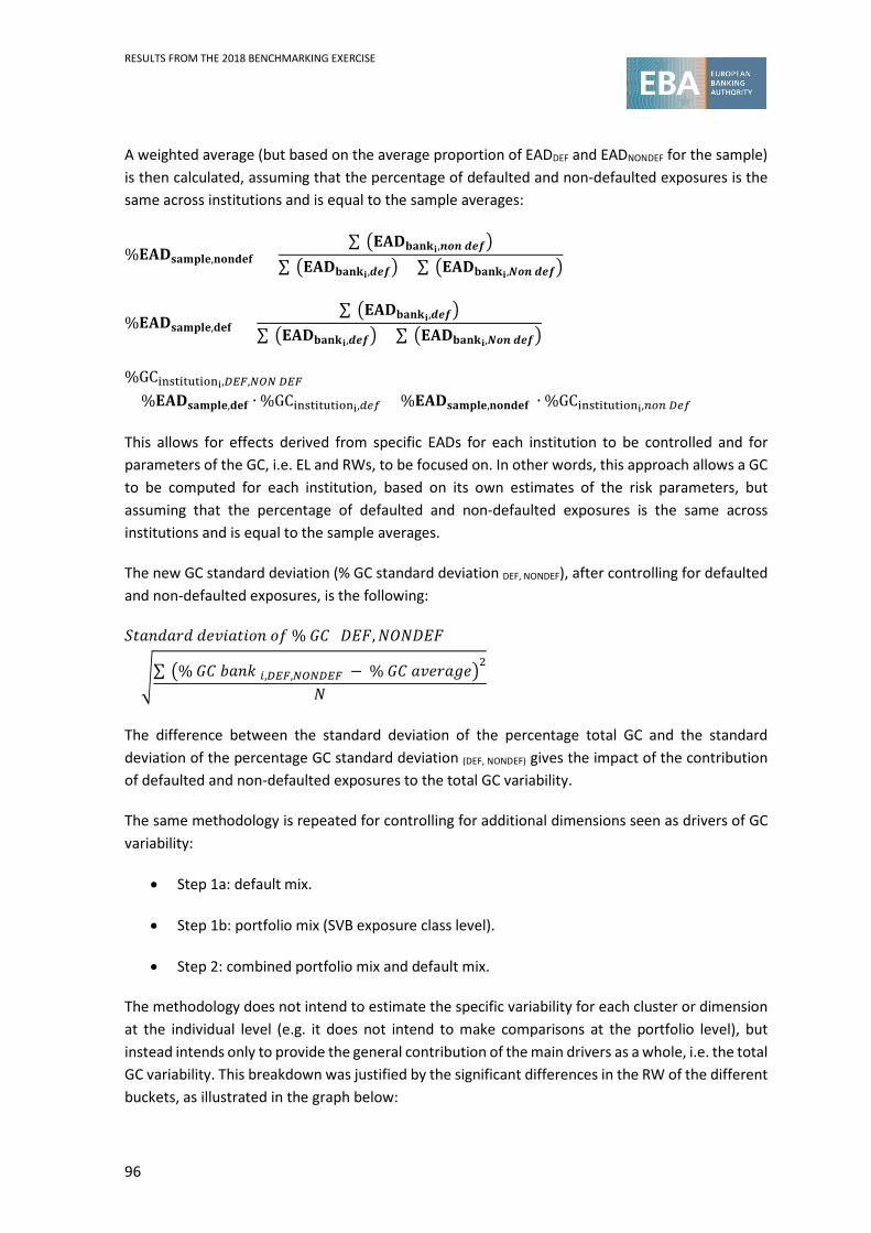
RESULTS FROM THE 2018 BENCHMARKING EXERCISE
96
A weighted average (but based on the average proportion of EADDEF and EADNONDEF for the sample) is then calculated, assuming that the percentage of defaulted and non-defaulted exposures is the same across institutions and is equal to the sample averages:
%𝐄𝐄𝐄𝐄𝐃𝐃𝐬𝐬𝐬𝐬𝐬𝐬𝐩𝐩𝐬𝐬𝐬𝐬,𝐧𝐧𝐧𝐧𝐧𝐧𝐧𝐧𝐬𝐬𝐧𝐧 = ∑ �𝐄𝐄𝐄𝐄𝐃𝐃𝐛𝐛𝐬𝐬𝐧𝐧𝐛𝐛𝐢𝐢,𝒃𝒃𝒏𝒏𝒃𝒃 𝒅𝒅𝑫𝑫𝒅𝒅�
∑ �𝐄𝐄𝐄𝐄𝐃𝐃𝐛𝐛𝐬𝐬𝐧𝐧𝐛𝐛𝐢𝐢,𝒅𝒅𝑫𝑫𝒅𝒅� + ∑ �𝐄𝐄𝐄𝐄𝐃𝐃𝐛𝐛𝐬𝐬𝐧𝐧𝐛𝐛𝐢𝐢,𝑵𝑵𝒏𝒏𝒃𝒃 𝒅𝒅𝑫𝑫𝒅𝒅�
%𝐄𝐄𝐄𝐄𝐃𝐃𝐬𝐬𝐬𝐬𝐬𝐬𝐩𝐩𝐬𝐬𝐬𝐬,𝐧𝐧𝐬𝐬𝐧𝐧 = ∑ �𝐄𝐄𝐄𝐄𝐃𝐃𝐛𝐛𝐬𝐬𝐧𝐧𝐛𝐛𝐢𝐢,𝒅𝒅𝑫𝑫𝒅𝒅�
∑ �𝐄𝐄𝐄𝐄𝐃𝐃𝐛𝐛𝐬𝐬𝐧𝐧𝐛𝐛𝐢𝐢,𝒅𝒅𝑫𝑫𝒅𝒅�+ ∑ �𝐄𝐄𝐄𝐄𝐃𝐃𝐛𝐛𝐬𝐬𝐧𝐧𝐛𝐛𝐢𝐢,𝑵𝑵𝒏𝒏𝒃𝒃 𝒅𝒅𝑫𝑫𝒅𝒅�
%GCinstitutioni,𝐷𝐷𝐷𝐷𝐷𝐷,𝑁𝑁𝑁𝑁𝑁𝑁 𝐷𝐷𝐷𝐷𝐷𝐷 = %𝐄𝐄𝐄𝐄𝐃𝐃𝐬𝐬𝐬𝐬𝐬𝐬𝐩𝐩𝐬𝐬𝐬𝐬,𝐧𝐧𝐬𝐬𝐧𝐧 ∙ %GCinstitutioni,𝑑𝑑𝑎𝑎𝑑𝑑 + %𝐄𝐄𝐄𝐄𝐃𝐃𝐬𝐬𝐬𝐬𝐬𝐬𝐩𝐩𝐬𝐬𝐬𝐬,𝐧𝐧𝐧𝐧𝐧𝐧𝐧𝐧𝐬𝐬𝐧𝐧 ∙ %GCinstitutioni,𝑏𝑏𝑛𝑛𝑏𝑏 𝐷𝐷𝑎𝑎𝑑𝑑
This allows for effects derived from specific EADs for each institution to be controlled and for parameters of the GC, i.e. EL and RWs, to be focused on. In other words, this approach allows a GC to be computed for each institution, based on its own estimates of the risk parameters, but assuming that the percentage of defaulted and non-defaulted exposures is the same across institutions and is equal to the sample averages.
The new GC standard deviation (% GC standard deviation DEF, NONDEF), after controlling for defaulted and non-defaulted exposures, is the following:
𝑆𝑆𝑡𝑡𝑡𝑡𝑏𝑏𝑆𝑆𝑡𝑡𝑆𝑆𝑆𝑆 𝑆𝑆𝑑𝑑𝑑𝑑𝑑𝑑𝑡𝑡𝑡𝑡𝑑𝑑𝑡𝑡𝑏𝑏 𝑡𝑡𝑜𝑜 % 𝐺𝐺𝐺𝐺 (𝐸𝐸𝐸𝐸𝐷𝐷,𝑁𝑁𝑁𝑁𝑁𝑁𝐸𝐸𝐸𝐸𝐷𝐷)
= �∑ �% 𝐺𝐺𝐺𝐺 𝑏𝑏𝑡𝑡𝑏𝑏𝑏𝑏 𝑖𝑖,𝐷𝐷𝐷𝐷𝐷𝐷,𝑁𝑁𝑁𝑁𝑁𝑁𝐷𝐷𝐷𝐷𝐷𝐷 − % 𝐺𝐺𝐺𝐺 𝑡𝑡𝑑𝑑𝑑𝑑𝑆𝑆𝑡𝑡𝑎𝑎𝑑𝑑�2
𝑁𝑁
The difference between the standard deviation of the percentage total GC and the standard deviation of the percentage GC standard deviation (DEF, NONDEF) gives the impact of the contribution of defaulted and non-defaulted exposures to the total GC variability.
The same methodology is repeated for controlling for additional dimensions seen as drivers of GC variability:
• Step 1a: default mix.
• Step 1b: portfolio mix (SVB exposure class level).
• Step 2: combined portfolio mix and default mix.
The methodology does not intend to estimate the specific variability for each cluster or dimension at the individual level (e.g. it does not intend to make comparisons at the portfolio level), but instead intends only to provide the general contribution of the main drivers as a whole, i.e. the total GC variability. This breakdown was justified by the significant differences in the RW of the different buckets, as illustrated in the graph below:

RESULTS FROM THE 2018 BENCHMARKING EXERCISE
97
• Portfolio mix:
Figure 51: RW dispersion (delta Q3 – Q1) of the different SVB exposure classes (defaulted and non-defaulted exposures)
0%
10%
20%
30%
40%
50%
60%
LCOR INST CGCB
0%
10%
20%
30%
40%
50%
60%
70%
80%
CORP MORT SMEC SMER

RESULTS FROM THE 2018 BENCHMARKING EXERCISE
98
• Portfolio and default mix:
Figure 52: RW dispersion (delta Q3 – Q1) for the different SVB exposure classes and default status (HDPs and LDPs)
0%
20%
40%
60%
80%
100%
120%
140%
LCOR CGCB INST LCOR CGCB INST
Default Non-default
0%
20%
40%
60%
80%
100%
120%
140%
160%
180%
CORP MORT SMEC SMER CORP MORT SMEC SMER
Default Non-default

RESULTS FROM THE 2018 BENCHMARKING EXERCISE
99
Analysis of IRB parameters for common counterparties
Institutions were instructed to provide risk parameters for a predefined list of counterparties, of which most are identified using the LEI71 as a unique and internationally accepted identifier. Table 15 gives the main statistics on the sample of counterparties. Note that the counterparties treated under SLSC are not shown in this table.
Table 15: Number of counterparties in the common counterparty analysis, by regulatory approach
Count No LEI
Total AIRB FIRB Total AIRB FIRB LC 15327 5109 5109 1242 414 414 INST 864 432 432 1242 33 33 GG 378 189 189 1242 183 183
The list of counterparties has been updated in comparison with that used in the 2017 LDP exercise, and the main changes were the deletion of counterparties that were obsolete and the addition of new counterparties, to increase representativeness at country level. Those changes have a limited impact overall, as shown in Figure 53.
Figure 53: Evolution of EAD by SVB portfolio and regulatory approach
The starting point for the analysis is the initial RW deviation, which provides an overall estimated deviation from the institution’s peers:
Deviation 1 represents the initial RW deviation: RW computed with the real parameters provided by the institutions (real maturity, real PD, real LGD) are compared with RW computed with the benchmark values (median PD of peers’ reported PD and median LGD of peers’
71 The LEI is a 20-character alphanumeric code that connects to key reference information that enables clear and unique identification of companies participating in global financial markets.
-
100,000
200,000
300,000
400,000
500,000
600,000
700,000
800,000
900,000
Previous BM Current BM Previous BM Current BM
AIRB FIRB
EUR
mill
ions
CGCB INST LCORP
RESULTS FROM THE 2018 BENCHMARKING EXERCISE
100
reported LGD) and the maturity fixed at 2.5 years [Dev1 = RiskWeight(M, PD, LGD) − RiskWeight(M = 2.5, b_PD, b_LGD)72]. This effect is calculated on the assumption that the changed parameters will not result in a shift of collateral.
By way of isolating the impact of the individual parameters, the following effects can be identified:
Deviation 2 represents the PD effect. RWs for a specific institution are computed with the benchmark values for all the parameters, excluding the PD, and these are compared with RWs computed with the benchmark values (median PD of peers’ reported PD) [Dev2 = RiskWeight(2.5, PD, b_LGD) − RiskWeight(2.5, b_PD,b_LGD)].
Deviation 3 represents the LGD effect. The RWs are computed with all the benchmark values, excluding the LGD, and are compared with RWs computed with the benchmark values reported by the institution [Dev3 = RiskWeight(2.5, b_PD, LGD) − RiskWeight(2.5, b_PD, b_LGD)].
Deviation 4 represents the maturity effect. The RWs are computed with all the benchmark values, excluding the maturity, and are compared with RWs computed with the values reported by the institution [Dev4 = RiskWeight(M, b_PD, b_LGD) − RiskWeight(2.5, b_PD, b_LGD)].
As the regulatory LGD estimated by the institution is used in the computation of these differences, the LGD effect also includes the impact of CRM. Therefore, the analysis has been repeated using the hypothetical senior unsecured LGD (without negative pledge) for the AIRB institutions only, where the values were provided assuming that the exposure to a given obligor was a senior unsecured exposure.
Deviation 5 represents the hypothetical LGD effect. RWs are computed with maturity fixed at 2.5 and PD fixed at benchmark values [Dev5 = RiskWeight(M = 2.5, b_PD, Hyp_LGD_ unsec) − RiskWeight(M = 2.5, b_PD, b_Hyp_LGD_unsec)]. This is the hypothetical LGD effect, which does not take the underlying collateral into account to achieve a uniform comparison.
72 The prefix ‘b_’ indicates that benchmarking values were used.

RESULTS FROM THE 2018 BENCHMARKING EXERCISE
101
Outturns (backtesting) approach
The analysis presents the ratios of the observed values to the estimated ones for comparable parameters. A result above 1 indicates an institution with an observed value higher than the institution’s estimate for the same (comparable) parameter. These ratios are calculated at the portfolio level73 for each institution. The complete definition of the data points collected can be found in Annex IV, Template C 103.00, of the ITS. In short, they were:
• PD (column 60): the PD used in the calculation of the RWA, excluding the effect of potential measures introduced in accordance with Article 458 of Regulation (EU) No 575/2013.
• LGD (column 130): the EAD-weighted own estimates of LGD or EAD-weighted regulatory LGD applied by the institution to the exposures to each portfolio shall be reported. The effect of measures introduced in accordance with Article 458 of Regulation (EU) No 575/2013 shall be excluded.
• DR1Y (column 190): the ratio of (i) the sum of the exposures (original exposure before applying the conversion factor measured at the reference date minus 1 year) that defaulted between the reference date minus 1 year and the reference date to (ii) the sum of the exposures (original exposure before applying the conversion factor measured at the reference date minus 1 year) that were non-defaulted at the reference date minus 1 year.
• DR5Y (column 200): the weighted average of the default rates observed in the past 5 years preceding the reference date (the weights to be used are the non-defaulted exposures).
• LR (column 210): the sum of credit risk adjustments and write-offs applied, within the year preceding the reference date, to exposures that were non-defaulted exactly 1 year before the reference date and that defaulted during the year preceding the reference date, divided by the sum of the EAD, measured exactly 1 year before the reference date, of the exposures that were non-defaulted exactly 1 year before the reference date and that defaulted during the year preceding the reference date.
• LR5Y (column 220): the EAD-weighted average of the loss rates observed in the past 5 years preceding the reference date shall be reported.
• RWA* (column 230): the hypothetical risk-weighted exposure amount, after applying the SME supporting factor, that results from the application of the maximum of PD and p*. For each obligor grade, 𝐩𝐩∗ is the smallest positive value satisfying the equation:
𝐩𝐩∗ + 𝚽𝚽−𝑫𝑫(𝐪𝐪) ∙ �𝐩𝐩∗ ∙ (𝑫𝑫 − 𝐩𝐩∗)
𝐧𝐧≥ 𝐃𝐃𝐃𝐃𝑫𝑫𝟏𝟏
NB: 𝑫𝑫𝑹𝑹𝑫𝑫𝒉𝒉 is NOT DR1Y, but the case-weighted default rate of the year preceding the reference date.
• RWA** (column 240): defined in a similar way as RWA*, but using the 𝐃𝐃𝐃𝐃𝟓𝟓𝟏𝟏 instead of 𝐃𝐃𝐃𝐃𝑫𝑫𝟏𝟏 (similarly with RWA*, 𝐃𝐃𝐃𝐃𝟓𝟓𝟏𝟏 is not equal to DR5Y).
73 Using portfolio ID (Annex I, template C 103.00 of the ITS).
RESULTS FROM THE 2018 BENCHMARKING EXERCISE
102
The persistence of institutions as outliers for both periods, i.e. the 1-year rate and the average of the past 5 years, and across comparable parameters can be examined by the CAs. However, there are a couple of caveats that should be kept in mind when doing this comparison, in particular for the comparison at the risk parameters level:
• Differences between the observed risk parameters used for prudential purposes and the data collected.
o The default rate collected is an exposure-weighted ratio, whereas the default rate used for the PD estimation should be an obligor ratio (further details are available in Section 5.3.2 of the Guidelines on PD and LGD estimation74).
o The loss rates collected uses accounting data as input. However, the loss used for prudential purposes should be the economic loss (and include considerations of collection-related costs, appropriate discounting, etc. Further details are available in Section 6.3.1 of the Guidelines on PD and LGD estimation).
• Differences between the rates collected and the long-run averages. PD and LGD estimates are required by Articles 180 and 181 of the CRR to be representative (PD) or at least equal (LGD) to the long-run average. However:
o The past (5) year(s) might not be representative of the long term (further details are available in Section 5.3.4 of the Guidelines on PD and LGD estimation).
o The long run average should be the arithmetic yearly average for the PD and a default weighted average for the LGD. The data collected are an exposure-weighted average of the DR for the DR5Y and an EAD-weighted average of the yearly LR for LR5Y (further details are available in Sections 5.3.3 and 6.3.3.2 of the Guidelines on PD and LGD estimation).
o The averages are not necessarily performed at the grade and pool level nor at the calibration level segment level, resulting in potential lack of homogeneity across time.
• Differences between the long-run averages and the risk parameters: o Both PD and LGD should incorporate a MoC (further details are available in
Section 4.4.3 of the Guidelines on PD and LGD estimation).
o LGD estimates should be appropriate for downturn conditions as per Article 181. The loss rates collected are not necessarily representative of downturn conditions.
Moreover, the data collected allowed only the comparison of PDs at the reference date (2017) with the default rate observed during the previous year (2016 – and also the average of the past 5 years), whereas it would be best to compare this default rate with the PD at the beginning of the observation period.
74 https://www.eba.europa.eu/documents/10180/2033363/Guidelines+on+PD+and+LGD+estimation+%28EBA-GL-2017-16%29.pdf/6b062012-45d6-4655-af04-801d26493ed0

RESULTS FROM THE 2018 BENCHMARKING EXERCISE
103
The RWA* and RWA** impact analysis also has a number of caveats, and the comparison with the RWA should be handled carefully:
• The two metrics aim only to provide an estimate of the potential magnitude of RWA changes under a specific scenario influenced by observed parameters. The data should be interpreted with caution, given the one-sided view of the analysis and some data quality constraints: possible positive variations (i.e., when PD is above p* or p**) and consequent compensation effects are not included (e.g. for a specific portfolio and specific rating grades, a possible underestimation of the PD and use of a higher PD to recalculate the RW, with a resulting decrease in the CET1 ratio, is not offset by a possible overestimation of the PD in another portfolio)
• The two metrics do not reflect regulatory measures or corrective actions in place that are having an impact on institutions’ capital requirements.
• Extrapolations to the total IRB credit risk portfolio cannot be made, because of the specific nature of HDP exposures.

RESULTS FROM THE 2018 BENCHMARKING EXERCISE
104
Country analysis
Common counterparties
All the analyses focus on the country of residence of the exposures, either looking at the whole portfolio (distribution and back-testing analysis), or at only selected exposures (common counterparty analysis). For this last analysis, the metric computed is the median value, on the counterparties of the selected country, of the interquartile range of the institutions’ estimates (RW) for each counterparty. In short, for each country ‘cy’, counterparty ‘ct’ belonging to this country and institution with RW estimates of those counterparties:
• 𝑄𝑄1𝑐𝑐𝑐𝑐 ∈ 𝑐𝑐𝑐𝑐�𝑄𝑄3�𝑅𝑅𝑅𝑅𝑏𝑏𝑏𝑏𝑏𝑏𝑏𝑏(𝑐𝑐𝑡𝑡)�𝑐𝑐𝑐𝑐 − 𝑄𝑄1�𝑅𝑅𝑅𝑅𝑏𝑏𝑏𝑏𝑏𝑏𝑏𝑏(𝑐𝑐𝑡𝑡)�𝑐𝑐𝑐𝑐�
• 𝑀𝑀𝑑𝑑𝑆𝑆𝑑𝑑𝑡𝑡𝑏𝑏𝑐𝑐𝑐𝑐 ∈ 𝑐𝑐𝑐𝑐�𝑄𝑄3�𝑅𝑅𝑅𝑅𝑏𝑏𝑏𝑏𝑏𝑏𝑏𝑏(𝑐𝑐𝑡𝑡)�𝑐𝑐𝑐𝑐 − 𝑄𝑄1�𝑅𝑅𝑅𝑅𝑏𝑏𝑏𝑏𝑏𝑏𝑏𝑏(𝑐𝑐𝑡𝑡)�𝑐𝑐𝑐𝑐�
• 𝑄𝑄3𝑐𝑐𝑐𝑐 ∈ 𝑐𝑐𝑐𝑐�𝑄𝑄3𝑏𝑏𝑏𝑏𝑏𝑏𝑏𝑏�𝑅𝑅𝑅𝑅(𝑐𝑐𝑡𝑡)�𝑐𝑐𝑐𝑐 − 𝑄𝑄1�𝑅𝑅𝑅𝑅𝑏𝑏𝑏𝑏𝑏𝑏𝑏𝑏(𝑐𝑐𝑡𝑡)�𝑐𝑐𝑐𝑐�
The analyses are based on the figures collected in template C 101.00, and only the counterparties for which the benchmark has been computed have been considered, and only the countries with more than 10 counterparties have been included in the charts.
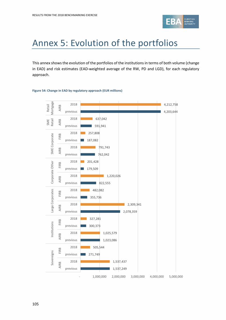
RESULTS FROM THE 2018 BENCHMARKING EXERCISE
105
Annex 5: Evolution of the portfolios
This annex shows the evolution of the portfolios of the institutions in terms of both volume (change in EAD) and risk estimates (EAD-weighted average of the RW, PD and LGD), for each regulatory approach.
Figure 54: Change in EAD by regulatory approach (EUR millions)
1,537,249
1,537,437
271,749
505,544
1,023,086
1,025,579
300,373
327,281
2,078,359
2,309,341
355,736
482,082
822,555
1,220,026
179,509
201,428
762,042
791,743
187,082
257,808
591,941
637,042
4,203,644
4,212,758
- 1,000,000 2,000,000 3,000,000 4,000,000 5,000,000
previous
2018
previous
2018
previous
2018
previous
2018
previous
2018
previous
2018
previous
2018
previous
2018
previous
2018
previous
2018
previous
2018
previous
2018
AIRB
FIRB
AIRB
FIRB
AIRB
FIRB
AIRB
FIRB
AIRB
FIRB
AIRB
AIRB
Sove
reig
nsIn
stitu
tions
Larg
e Co
rpor
ates
Corp
orat
e O
ther
SME
Corp
orat
eSM
ERe
tail
Reta
ilM
ortg
age

RESULTS FROM THE 2018 BENCHMARKING EXERCISE
106
Figure 55: Change in EAD-weighted RW by regulatory approach
8%
7%
3%
2%
24%
26%
21%
20%
46%
43%
48%
46%
48%
43%
58%
62%
41%
40%
63%
57%
25%
27%
13%
12%
0% 10% 20% 30% 40% 50% 60% 70%
previous
2018
previous
2018
previous
2018
previous
2018
previous
2018
previous
2018
previous
2018
previous
2018
previous
2018
previous
2018
previous
2018
previous
2018
AIRB
FIRB
AIRB
FIRB
AIRB
FIRB
AIRB
FIRB
AIRB
FIRB
AIRB
AIRB
Sove
reig
nsIn
stitu
tions
Larg
e Co
rpor
ates
Corp
orat
e O
ther
SME
Corp
orat
eSM
ERe
tail
Reta
ilM
ortg
age

RESULTS FROM THE 2018 BENCHMARKING EXERCISE
107
Figure 56: Change in EAD-weighted PD by regulatory approach
0.2%
0.1%
0.0%
0.0%
0.5%
0.5%
0.3%
0.2%
2.9%
2.8%
2.1%
3.6%
8.7%
6.1%
7.0%
5.8%
17.1%
15.1%
10.1%
9.2%
14.4%
13.3%
3.4%
3.0%
0.0% 2.0% 4.0% 6.0% 8.0% 10.0% 12.0% 14.0% 16.0% 18.0%
previous
2018
previous
2018
previous
2018
previous
2018
previous
2018
previous
2018
previous
2018
previous
2018
previous
2018
previous
2018
previous
2018
previous
2018AI
RBFI
RBAI
RBFI
RBAI
RBFI
RBAI
RBFI
RBAI
RBFI
RBAI
RBAI
RB
Sove
reig
nsIn
stitu
tions
Larg
e Co
rpor
ates
Corp
orat
e O
ther
SME
Corp
orat
eSM
ERe
tail
Reta
ilM
ortg
age

RESULTS FROM THE 2018 BENCHMARKING EXERCISE
108
Figure 57: Change in EAD-weighted LGD by regulatory approach
32.6%
29.0%
43.3%
44.5%
34.2%
35.3%
26.6%
28.0%
38.0%
36.8%
43.3%
42.7%
29.1%
28.4%
43.8%
42.0%
28.9%
27.3%
40.9%
41.1%
30.0%
30.4%
13.5%
14.0%
0.0% 10.0% 20.0% 30.0% 40.0% 50.0%
previous
2018
previous
2018
previous
2018
previous
2018
previous
2018
previous
2018
previous
2018
previous
2018
previous
2018
previous
2018
previous
2018
previous
2018
AIRB
FIRB
AIRB
FIRB
AIRB
FIRB
AIRB
FIRB
AIRB
FIRB
AIRB
AIRB
Sove
reig
nsIn
stitu
tions
Larg
e Co
rpor
ates
Corp
orat
e O
ther
SME
Corp
orat
eSM
ERe
tail
Reta
ilM
ortg
age

RESULTS FROM THE 2018 BENCHMARKING EXERCISE
109
Annex 6: Analysis by country of the counterparty
In contrast to previous SVB exercises, in which the country analysis was performed by the country of the CA of the institution, the country analysis presented in this section has been performed on the country of the counterparty (the residence of the obligor).
1. Distribution analysis
The following graphs show the RW assessment of the institutions, organised by the country of the common counterparty, for each of the seven SVB exposure classes, for non-defaulted exposures. Only those counterparties in countries where at least five institutions’ rate exposures included in the exercise are reported.
Although no statistical tests have been performed to confirm this hypothesis, the information in Figure 58 to Figure 64 seems to suggest that domestic institutions (for ‘domestic’ here we mean where the country of the CA of the institution, at the highest level of consolidation in the EU, is the same as the country of the residence of the counterparty) have a more consistent RW assessment of counterparties in their jurisdiction than non-domestic institutions. This can be seen by the fact that the RW dispersion for _DOM is generally narrower than for the full sample of institutions assessing the counterparty in each country. This effect may show that there is still significant heterogeneity remaining between jurisdictions, whereas modelling practices within each jurisdiction are much more streamlined. On the other hand, this pattern may also be explained by the fact that domestic institutions usually have more rated counterparties in their jurisdiction than non-domestic institutions do. As such, fewer data points usually imply that it is harder to obtain a robust RW assessment. It should, however, be stressed that these are tentative conclusions, and further analysis is needed to confirm this hypothesis.
That said, it is key to mention that the information on the residence of the counterparty has been taken into account, as an additional dimension, in the determination of outlier institutions in the SVB analysis.

RESULTS FROM THE 2018 BENCHMARKING EXERCISE
110
Figure 58: RW distribution for sovereign non-defaulted exposures, by country of residence of the portfolio
Figure 59: RW distribution for corporate non-defaulted exposures, by country of residence of the portfolio
Figure 60: RW distribution for non-defaulted exposures to institutions, by country of residence of the portfolio
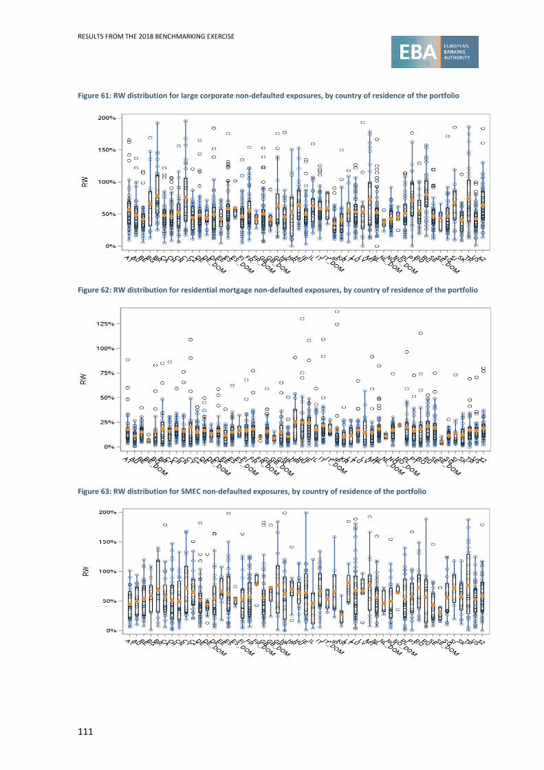
RESULTS FROM THE 2018 BENCHMARKING EXERCISE
111
Figure 61: RW distribution for large corporate non-defaulted exposures, by country of residence of the portfolio
Figure 62: RW distribution for residential mortgage non-defaulted exposures, by country of residence of the portfolio
Figure 63: RW distribution for SMEC non-defaulted exposures, by country of residence of the portfolio

RESULTS FROM THE 2018 BENCHMARKING EXERCISE
112
Figure 64: RW distribution for SMER non-defaulted exposures, by country of residence of the portfolio
2. LDPs: common counterparties
In order to get a view on the dispersion in the institution’s risk assessment across counterparties in the same jurisdiction, Figure 65 and Figure 66 show the median, the first and third quartile of the interquartile range of the institutions’ RW estimates for each counterparty (see the formula in Annex 4).
For this analysis, only those key metrics on the distribution of the interquartile range are displayed, given that the distribution is based on the common counterparties and not on the institutions participating in this exercise (the sample size is therefore much bigger than other analyses). In short, this allows the breakdown of the total RW deviation shown in Section 2.2 into buckets of countries of counterparties.
The metrics are consistent with the results displayed in Section 2.2, with RW deviations being around 20%. This analysis shows, however, some heterogeneity in the variability of estimates between countries. Other than that, no clear patterns can be observed as regards the heterogeneity of these RW assessments by the different institutions.
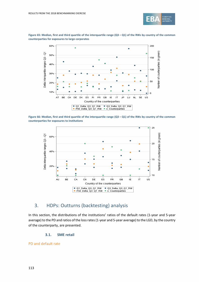
RESULTS FROM THE 2018 BENCHMARKING EXERCISE
113
Figure 65: Median, first and third quartile of the interquartile range (Q3 – Q1) of the RWs by country of the common counterparties for exposures to large corporates
Figure 66: Median, first and third quartile of the interquartile range (Q3 – Q1) of the RWs by country of the common counterparties for exposures to institutions
3. HDPs: Outturns (backtesting) analysis
In this section, the distributions of the institutions’ ratios of the default rates (1-year and 5-year average) to the PD and ratios of the loss rates (1-year and 5-year average) to the LGD, by the country of the counterparty, are presented.
3.1. SME retail
PD and default rate

RESULTS FROM THE 2018 BENCHMARKING EXERCISE
114
The outturns (backtesting) approach shows that, for all exposure countries, the third quartile of the ratios of the default rate for the past year to the PD is below 1, which is in line with the findings set out in Section 2.3. These results are similar for the ratios of the 5-year average loss rate to the LGD for all countries but one. That is, in general, the estimated values (PDs) are higher than the observed values (default rates) for the past 5 years.
Although the distributions of the average ratio (DR/PD) by country are very similar, the backtesting results for the average loss rate for the past 5 years are higher than those for the past year, which is in line with the aggregated figures in Figure 67 and suggests that, after an economic downturn that affected many countries, loss rates are decreasing.
Figure 67: Comparison of the PD and the default rate (past year and past 5 years), for the SME retail portfolio, for non-defaulted exposures, for the AIRB approach, by country of residence of the counterparties (with at least five institutions)
LGD and loss rate
Similarly to the results above, the backtesting approach shows that, for all exposure countries, in the third quartile, the ratios of the loss rate (both for the past year and for the past 5 years) to the

RESULTS FROM THE 2018 BENCHMARKING EXERCISE
115
LGD are below 1. That is, in general, the estimated values (LGDs) for SME retail exposures are higher than the observed values (loss rates) over the past 5 years.
In addition, when comparing the distribution of the average ratios (LR/LGD) across countries, the results suggest that the loss rates are either increasing or are stable over the past 5 years. The 5-year average is (for all countries but one) less than 50% of estimated LGD. With regard to the loss rate for the past year, there are more countries with observed losses greater than 50% of the estimated LGD. In fact, the results appear to be very low and this could result from data quality issues in the submission of data for this SVB exercise.
Figure 68: Comparison of the LGD and the loss rate (past year and past 5 years), for the SME retail portfolio, for non-defaulted exposures, for the AIRB approach, by country of residence of the counterparties (with at least five institutions)
3.2. SME corporate
PD and default rate
For the SME corporate exposures, the backtesting results can be compared for different regulatory approaches. This comparison shows that, across countries, the backtesting results related to the
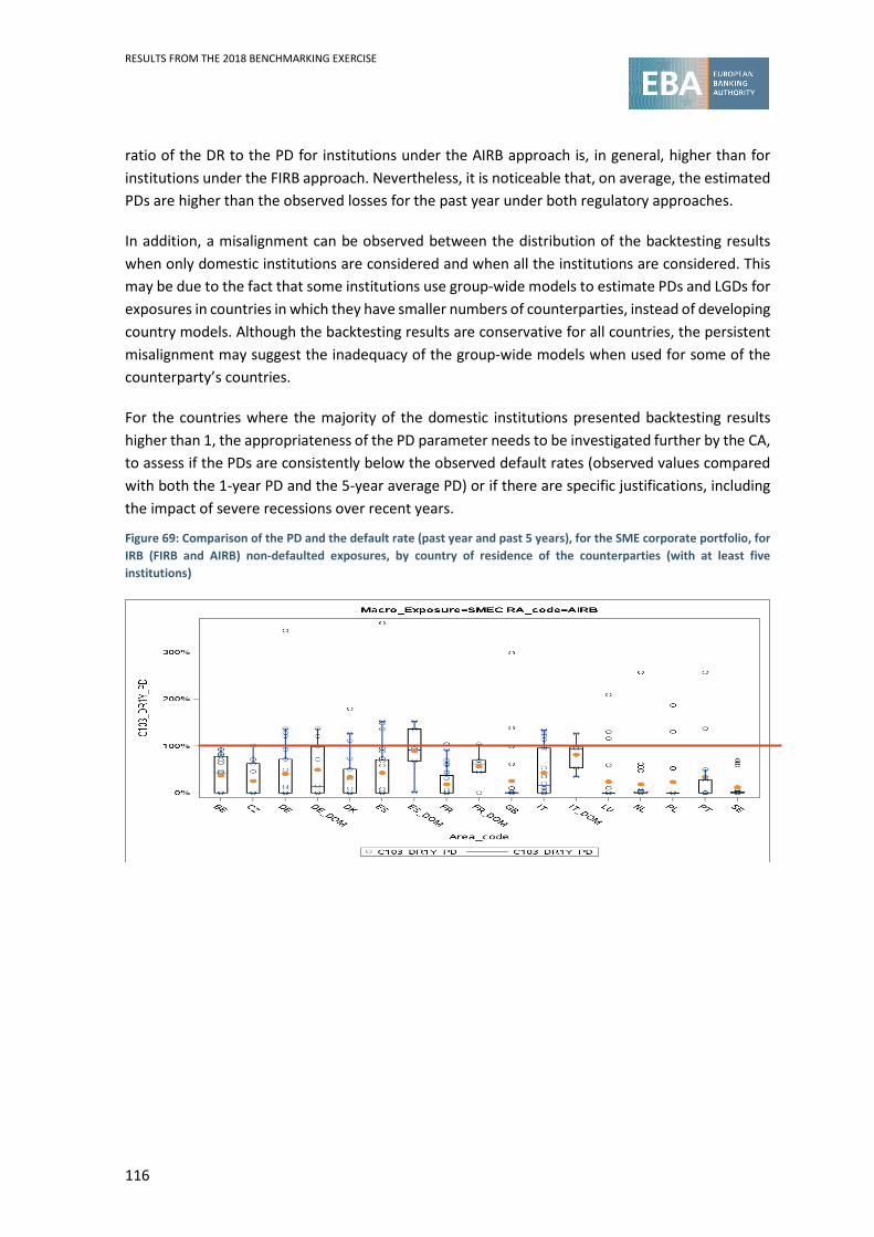
RESULTS FROM THE 2018 BENCHMARKING EXERCISE
116
ratio of the DR to the PD for institutions under the AIRB approach is, in general, higher than for institutions under the FIRB approach. Nevertheless, it is noticeable that, on average, the estimated PDs are higher than the observed losses for the past year under both regulatory approaches.
In addition, a misalignment can be observed between the distribution of the backtesting results when only domestic institutions are considered and when all the institutions are considered. This may be due to the fact that some institutions use group-wide models to estimate PDs and LGDs for exposures in countries in which they have smaller numbers of counterparties, instead of developing country models. Although the backtesting results are conservative for all countries, the persistent misalignment may suggest the inadequacy of the group-wide models when used for some of the counterparty’s countries.
For the countries where the majority of the domestic institutions presented backtesting results higher than 1, the appropriateness of the PD parameter needs to be investigated further by the CA, to assess if the PDs are consistently below the observed default rates (observed values compared with both the 1-year PD and the 5-year average PD) or if there are specific justifications, including the impact of severe recessions over recent years.
Figure 69: Comparison of the PD and the default rate (past year and past 5 years), for the SME corporate portfolio, for IRB (FIRB and AIRB) non-defaulted exposures, by country of residence of the counterparties (with at least five institutions)
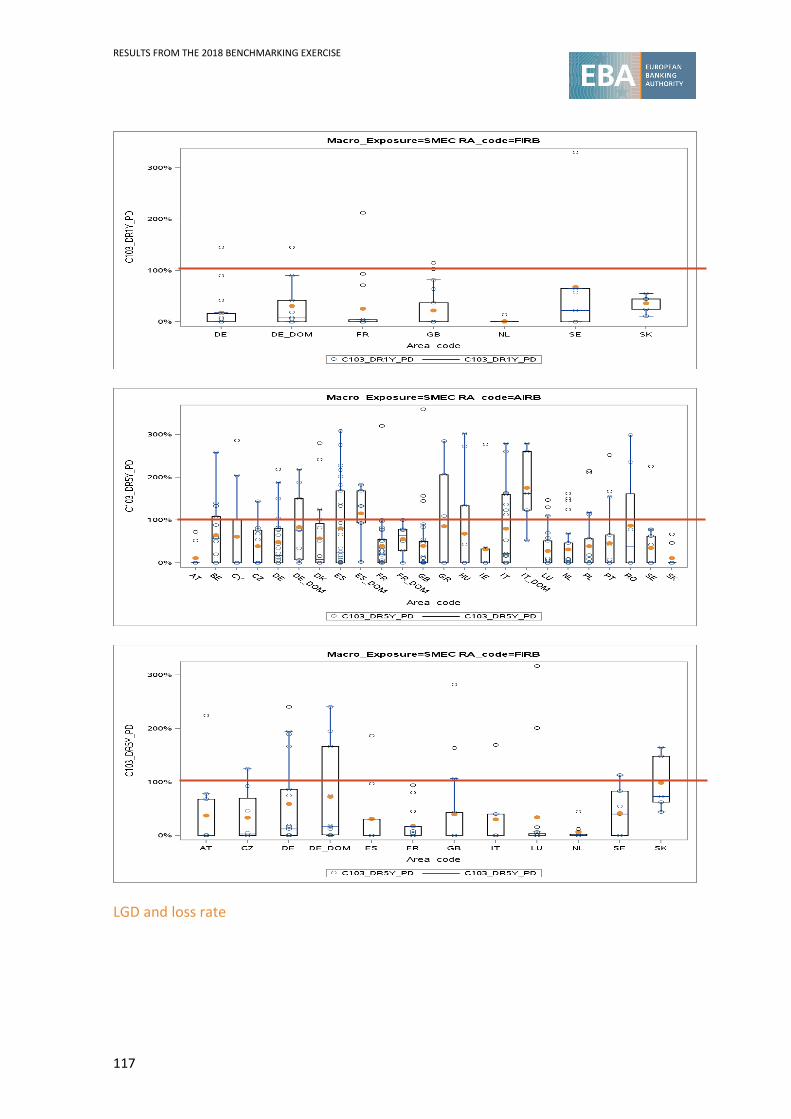
RESULTS FROM THE 2018 BENCHMARKING EXERCISE
117
LGD and loss rate

RESULTS FROM THE 2018 BENCHMARKING EXERCISE
118
Regarding the loss rates, the institutions, under both the AIRB and the FIRB approaches, for the SME corporate portfolio, show conservative75 figures. In addition, it seems that for SME corporates the loss rates are decreasing over time and/or the LGDs are being adjusted, as the 5-year average ratios are, in general, equal or higher to the past year ratios.
Figure 70: Comparison of the LGD and the loss rate (past year and past 5 years), for the SME corporate portfolio, for IRB (FIRB and AIRB) non-defaulted exposures, by country of residence of the counterparties (with at least five institutions)
3.3. Corporate-other
PD and default rate
Regarding the corporate-other portfolios, the misalignment between the backtesting results for all institutions and only for domestic institutions, especially under the AIRB approach, are observable.
75 Note again that this has to be interpreted with caution as the loss rate is based on estimations. A case-by-case analysis should therefore complement these observations.

RESULTS FROM THE 2018 BENCHMARKING EXERCISE
119
Moreover, the backtesting results regarding the PD estimates, although they are conservative, appear to be higher than the results regarding LGD estimates, under the AIRB approach.
Figure 71: Comparison of the PD and the default rate (past year and past 5 years), for the corporate-other portfolio, for IRB (FIRB and AIRB) non-defaulted exposures, by country of residence of the counterparties (with at least five institutions)

RESULTS FROM THE 2018 BENCHMARKING EXERCISE
120
LGD and loss rate
The SVB results show that the estimated LGDs for corporate-other portfolios are higher than the observed loss rates for the past 5 years, independently of the exposures’ country and the regulatory approach followed by the institutions.
Figure 72: Comparison of the LGD and the loss rate (past year and past 5 years), for the corporate-other portfolio, for IRB (FIRB and AIRB) non-defaulted exposures, by country of residence of the counterparties (with at least five institutions)

RESULTS FROM THE 2018 BENCHMARKING EXERCISE
121
3.4. Residential mortgages
PD and default rate
The outturns approach for residential mortgages shows that, in the third quartile, the ratios of the default rate to the PD, for both the past year and the past 5 years, are below 1, except for two countries and when considering only domestic institutions. That is, in general, the estimated PDs are higher than the default rates observed over the past 5 years. In particular, for the past year it can be seen that the interquartile range and the average by country are lower than when considering the 5-year average loss rates. As in other portfolios, this suggests that the default rates decreased in the past year, as the past 5 years saw economic downturns in many EU countries.
Figure 73: Comparison of the PD and the default rate (past year and past 5 years), for the residential mortgages portfolio, for IRB AIRB non-defaulted exposures, by country of residence of the counterparties (with at least five institutions)

RESULTS FROM THE 2018 BENCHMARKING EXERCISE
122
LGD and loss rate
The outturns approach regarding the comparison between the observed loss rates and the estimated LGDs, shows conservative results as the distributions of the ratios by exposure country as being below 1. In general, the estimated LGDs are higher than the loss rates reported in recent years. This is consistent with the fact that the CRR requires LGDs to reflect downturn conditions.
When comparing the results for the past year with those for the past 5 years, the LGD interquartile ranges for the past year and the past 5 years show similar variability.
Figure 74: Comparison of the LGD and the loss rate (past year and past 5 years), for the residential mortgages portfolio, for IRB AIRB non-defaulted exposures, by country of residence of the counterparties (with at least five institutions)

RESULTS FROM THE 2018 BENCHMARKING EXERCISE
123

EUROPEAN BANKING AUTHORITY
Floor 46 One Canada Square, London E14 5AA
Tel. +44 (0)207 382 1776 Fax: +44 (0)207 382 1771 E-mail: [email protected]
http://www.eba.europa.eu