Earthquake rupture process recreatedfrom a natural fault surfaceTom Parsons1 and Diane L. Minasian1

1U.S. Geological Survey, Menlo Park, California, USA

Abstract What exactly happens on the rupture surface as an earthquake nucleates, spreads, and stops? Wecannot observe this directly, and models depend on assumptions about physical conditions and geometry atdepth. We thus measure a natural fault surface and use its 3-D coordinates to construct a replica at 0.1mresolution to obviate geometry uncertainty. We can recreate stick-slip behavior on the resulting finite elementmodel that depends solely on observed fault geometry. We clamp the fault together and apply steady statetectonic stress until seismic slip initiates and terminates. Our recreated M~1 earthquake initiates at contactpoints where there are steep surface gradients because infinitesimal lateral displacements reduce clampingstress most efficiently there. Unclamping enables accelerating slip to spread across the surface, but the faultsoon jams up because its uneven, anisotropic shape begins to juxtapose new high-relief sticking points. Thesecontacts would ultimately need to be sheared off or strongly deformed before another similar earthquake couldoccur. Our model shows that an important role is played by fault-wall geometry, although we do not includeeffects of varying fluid pressure or exotic rheologies on the fault surfaces. We extrapolate our results to largefault systems using observed self-similarity properties and suggest that larger ruptures might begin and end ina similar way, although the scale of geometrical variation in fault shape that can arrest a rupture necessarilyscales with magnitude. In other words, fault segmentation may be a magnitude-dependent phenomenon andcould vary with each subsequent rupture.

1. Introduction

Important questions about the earthquake rupture process remain unanswered, complicating our ability toforecast them [e.g., Field et al., 2014]. There is some apparent predictability regarding where earthquakesbegin and end [e.g., Wesnousky, 2006], but uncertainties are large enough that hazard studies do not neces-sarily assume that earthquakes will repeat themselves within segment boundaries [Field and Page, 2011]. Infact, debate persists whether individual faults host repeated characteristic magnitude earthquakes or follow apower law distribution [e.g., Schwartz and Coppersmith, 1984;Wesnousky, 1994; Stein and Newman, 2004; Pageet al., 2011; Page and Felzer, 2015]. Here we recreate a fault and its earthquakes numerically, with a modeltaken directly from a natural surface (Figure 1), so that we can explore the consequences of its shape and gaindirect insight into earthquake initiation and arrest.

We measure an exposed fault with ground-based lidar and use the 3-D point cloud to build a finite elementreplica (Figure 2). This model naturally exhibits stick-slip behavior when stress is applied in its rake direction,behavior that is difficult to capture numerically using randomized elastic surfaces, although successful resultshave been achieved with discrete element models [e.g., Fournier and Morgan, 2012]. In the context of ourmodel, we define stick slip as the fault resisting applied stress (sticking) as it begins a nucleation process(infinitesimal slip), until finally, significant displacement occurs at relatively high velocity (slipping). We can-not, at this stage, conduct a fully dynamic rupture simulation while simultaneously incorporating the fullcomplexity of a natural fault surface because of computational limitations. Instead, rupture evolution isapproximated by very short time steps that are solved statically. In this way we can observe quasi-dynamicfeatures such as relative slip speed and the spatial distribution of preseismic slip that occur as a consequenceof fault geometry. Our calculations are performed in the elastic limit, and no plastic yield is modeled, which isthemain limitation at small scales and for the largest earthquakes. If we accept this simulation as a reasonableapproximation of the natural process, then we discover which features of the fault surface encourage initiationof earthquake slip, those that act to arrest it, and the influence of fault roughness on asperities. Earthquakefaults are known to exhibit self-similarity and scale invariant complexity, which contextualizes our resultsto larger, and thus dangerous fault zones.

PARSONS AND MINASIAN NUMERICAL FAULT MODEL FROM LIDAR 7852

PUBLICATIONSJournal of Geophysical Research: Solid Earth

RESEARCH ARTICLE10.1002/2015JB012448

Key Points:• In situ fault surface measured• Numerical model made directly frompoint cloud

• Earthquake rupture recreated onmodel fault

Correspondence to:T. Parsons,tparsons@usgs.gov

Citation:Parsons, T., and D. L. Minasian (2015),Earthquake rupture process recreatedfrom a natural fault surface, J. Geophys.Res. Solid Earth, 120, 7852–7862,doi:10.1002/2015JB012448.

Received 13 AUG 2015Accepted 23 OCT 2015Accepted article online 27 OCT 2015Published online 27 NOV 2015

Published 2015. This article is a U.S.Government work and is in the publicdomain in the USA.

We recognize that a natural fault in situ is a far more complex system than we can replicate numerically atthis time. However, we can experiment to see what happens when a numerical representation of a naturalfault is subjected to applied stress. This approach can allow an assessment of the potential role of surfaceheterogeneity on slip propagation and nucleation.

2. Observations

The Corona Heights fault is located within the city of San Francisco, CA (Figure 1), and it cuts throughan early Jurassic [Murchey and Jones, 1984], massive radiolarian chert unit of the Franciscan Formation[Schlocker, 1974]. The timing of faulting on the dextral [Kirkpatrick et al., 2013] Corona Heights fault is unde-termined, but we know that it was exposed during quarrying operations by George and Harry Gray thatbegan in 1909 and ceased shortly after the murder of George Gray in 1914 over a refusal to pay back wages[Bevk, 2013]. The fault thus has well-preserved corrugation and slickenside features, making it ideal fordetailed study [Candela et al., 2011, 2012; Kirkpatrick et al., 2013; Kirkpatrick and Brodsky, 2014]. TheCorona Heights fault offset is estimated to be ~50m or less [Kirkpatrick and Brodsky, 2014]. Natural fault sur-faces tend to have anisotropic roughness [Brown and Scholz, 1985; Power et al., 1987], which is true in thecase of the Corona Heights fault [Kirkpatrick and Brodsky, 2014].

Figure 1. The yellow star shows the location of the Corona Heights fault in the city of San Francisco, CA, USA. (a) A photoof the Corona Heights fault surface that was scanned with ground-based lidar. (b) The resulting point cloud was usedto make a 0.1 m spaced digital elevation model (DEM) that defined node locations of the (c) finite element model(see also Figure 2).

Journal of Geophysical Research: Solid Earth 10.1002/2015JB012448

PARSONS AND MINASIAN NUMERICAL FAULT MODEL FROM LIDAR 7853

We use a tripod mounted Riegl Z210 laser scanner system (lidar) to develop a 3-D model of the CoronaHeights fault. Multiple scans are collected to fill in locations not directly in the line of sight of the laserand to expand the range and density of the point data. Data are collected at a rate of 8000 points persecond, scanning a range of 336° in the horizontal direction and 40° from the horizontal in the verticaldirection. We conduct scans over a range from 1mm to 10 cm resolution. Processing is performed usingI-SiTE software specifically designed to handle laser scan data. Point data are filtered to remove extraneouslaser returns from the point clouds. Points reflected from vegetation are manually cropped from eachof the clouds, and topographic filters that select the lowest level in the point clouds are also used toremove vegetation.

We use full-resolution processed lidar points to construct a regularly spaced digital elevation model (DEM)(Figure 1). We perform a grid search to find the horizontal plane that minimizes long-wavelength relief onthe fault surface and rotate the coordinate system so that plane is horizontal. The original orientation of thefault when it was active is unknown, but it has a right-lateral rake; we rotate the DEM model so that thex direction is parallel to the observed slip direction as interpreted from striations (27° rotation counterclock-wise about our z axis) [Kirkpatrick and Brodsky, 2014].

3. Model Development

The primary goal of our modeling is to assess the role that fault geometry/topography plays in generatingand resisting earthquakes. The advantage of replicating a real fault surface in 3-D means that no geometricalassumptions are made for scales equal to or above the model node spacing. However, a number of tradeoffsalso need to be made because a 3-D finite element model of a natural surface requires a very large number of

Figure 2. Finite elementmodel showing the applied displacements/forces. The 2.5m thick upper plate is made transparentso that its inverse, a 2.5 m thick lower plate, and the fault surface can be seen. The model is clamped by moving the upperplate down by 0.01m. Fault surface slip was caused by fixing the lower plate base and applying a ramped force on theupper plate in the �x direction. No lateral slip was imposed, only stress. In Figure 2b a close-up view of the fault surfacemesh is shown to illustrate the resolution (0.1 m node spacing).

Journal of Geophysical Research: Solid Earth 10.1002/2015JB012448

PARSONS AND MINASIAN NUMERICAL FAULT MODEL FROM LIDAR 7854

element nodes that have complex contact interactions. Therefore, as described below, a fully dynamic solu-tion or one that includes exotic friction and mobile pore fluids remains outside our computational resources.

We subsample the DEM generated from lidar measurements to a 0.1m spaced grid, which represents theminimum node spacing that can reasonably be meshed into a finite element model under our computermemory constraints. All calculations are made with the commercial ANSYS© software that enables largedeformation (finite strain), although we treat rocks as elastic materials here to limit the number of parametersrequired. We begin with a meshed, initially rectangular prism (length 38m, height 18m, depth 2.5m), andthen move surface nodes to positions described by the DEM to recreate the fault surface. The inverse is doneto another prism to create the upper plate (also 2.5m thick) so that they fit together exactly (Figure 2). Wheretwo sides of an actual fault are observed in detail, they mirror each other at lateral dimensions greater than0.02m [Power and Tullis, 1992], which is well below our 0.1m spacing.

Both fault faces are draped with zero-thickness contact elements that obey a Coulomb failure criterion; wetested uniform friction coefficients ranging from μ= 0.2 to μ= 0.8. We fixed Poisson’s ratio to 0.25 for allexperiments. The total fault area in the model is 563.6m2. The model has 313,832 elastic elements character-ized by a soft Young’s modulus of E= 5GPa; fault zones are expected to have reduced Young’s modulibecause of crushing and fracturing [Gudmundsson, 2004], with the approximate value of clays and othercohesive/plastic materials [Kezdi, 1974]. As a linear constant, the absolute value of Young’s modulus is onlyimportant in terms of relating elastic strain (ε) to stress (σ) as ε= σ/E, but stress in our model comes froman applied steady state force. In other words, a higher Young’s modulus results in the same behavior butat higher stress levels.

We generate stick-slip behavior by compressing the fault together (uz= 0.01m) to create fault-normal(clamping) stress, which when combined with friction, acts to resist fault slip according to the Coulomb failurecriterionCFF ≡ τfj j þ μ σn � pð Þ, where τf is shear stress in the rake direction, σn is the stress normal to the faultplane, and p is pore fluid pressure (not explicitly modeled in this study). Sensitivity of failure to clamping canbe assessed by the coefficient of friction (μ) or normal stress; we vary friction coefficient rather than uzdisplacement to avoid unduly affecting the shape of the fault surface before slip can occur. Changing thefriction coefficient can account for pore fluid pressure variation in a rudimentary way if fluids are confinedwithin the fault, or in fault parallel cracks that are pressurized uniformly by normal stresses [e.g., Rice, 1992;Scholz, 2002]. Given the significant topography of our modeled fault surface, we recognize that the role ofpore fluids is necessarily simplified by our model. Finally, we assume that the far-field stress state at themodelboundaries does not vary over the spatial scale of the model (38m by 18m).

The model lower plate is fixed in all directions, and the model upper plate is loaded in the �x direction toencourage dextral slip on the fault surface; a linear time-ramped force is applied across the entire top surfaceof themodel from zero until the earthquake is completed. Themaximum stress reached is 0.77 � 106 N appliedon a unit area, which sums to 77.0MPa of applied stress to the system; this is the stress applied to the modelexterior, which has a slightly greater area than the embedded fault interface (Figure 2). This thresholddepends linearly on the values of Young’s modulus and the coefficient of friction and simply increases as theydo. Model results are shown with relatively low values of μ= 0.2 and E= 5.0 GPa. The fault mostly resistsslipping prior to the maximum stress threshold, and then breaks free, generating a small earthquake. Forceis accumulated at a uniform rate throughout the simulation, replicating steady state tectonic stressing.

In other words, loading is simulating tectonic stress with shear applied on one exterior face of the model,parallel to the fault slip direction, while the opposing face is held fixed (Figure 2). Stress is ramped up withtime as we expect it to in the real Earth. We also apply a small component of fault-normal compression tohold the fault together. Application of stress does not result in immediate, significant slip on the faultbecause there are multiple points of contact that resist slip because of their geometry. Thus, elastic strainbuilds in the fault walls and at resisting points on the fault. Competing with those resisting contact pointsare other, releasing zones where slip is encouraged. As will be discussed, it appears in the model thatearthquake initiation depends in part on the balance between sticking and sliding fault topography andthe ability of releasing points to organize into large patches of slip that can overcome resisting geometry.

The modeling we conduct is static rather than fully dynamic. This has two primary effects: (1) there is noaccounting for inertial influences on simulated earthquake rupture. In the real Earth, once the faulted mass

Journal of Geophysical Research: Solid Earth 10.1002/2015JB012448

PARSONS AND MINASIAN NUMERICAL FAULT MODEL FROM LIDAR 7855

begins to move, it has momentum that must be damped for the earthquake to cease. In our case, rupturebegins when the shear stress state exceeds resistance and ceases when the opposite is true. (2) We rampthe model forcing over time steps, but the time variable in our case only tracks the relative durations thatthe fault is in different stages of loading and slip. The absolute time scale is arbitrary and depends on therate that we apply force. This means we cannot give rupture velocity or discuss rupture preparation times inabsolute terms, but only over a normalized period. On the other hand, we have to estimate relatively fewparameters as compared with fully dynamic simulations [e.g., Duan and Oglesby, 2005; Xu et al., 2015], andthose that we do need (friction coefficient, Young’s modulus, force amplitude, and time step) all trade off

Figure 3. RecreatedM = 0.95 earthquake on the Corona Heights fault. In steps (a–c) the prerupture phase is shown, wheremost of the fault surface is locked (red shading in adjacent column). Gray areas are regions with no slip (locked). Nearcontact means that contact elements are beginning to open up as a result of slip. Offset can still occur in these areas, butnot as full frictional contact.

Figure 4. At step (d) low-magnitude slip begins around the fault edges and in areas of steep fault-surface topography(sliding areas are shaded orange in adjacent column). At steps (e–g) slip spreads in the rake direction, and areas withhighest slip experience opening (yellow shading) with slip ceasing there.

Journal of Geophysical Research: Solid Earth 10.1002/2015JB012448

PARSONS AND MINASIAN NUMERICAL FAULT MODEL FROM LIDAR 7856

linearly. The primary contribution from our modeling is thus quantifying the role of fault topography onrupture resistance, initiation, and termination.

4. Model Results

By replicating a natural fault surface, we can generate small (M~1.0), simulated earthquakes (Figures 3 and 4)without enforcing any special friction conditions to initiate or stop ruptures. Typically, a smooth frictionalsurface will slip/creep in direct proportion to applied forces in finite element models, and it is difficult toachieve spontaneous stick-sip behavior without predefining failure conditions [e.g., Lynch and Richards,2001; Xing et al., 2004; Coon et al., 2011]. This is because it is a lower energy solution for a model fault to creepcompared with distorting the entire model volume surrounding a locked fault.

We apply uniform compression across the natural fault and then begin steady state forcing in the rakedirection to replicate tectonic stress accumulation (Figure 2) as frictional resistance is overcome. The faultslips very slowly as stress builds up and then accelerates rapidly during the final seismic stages (Figure 4).The areas that slip initially are small (on the order of a few square centimeters), and they slip less than 1mm(Figure 3). Such small slips would likely not be detectable with seismographs. Most of the fault surfaceaccumulates a small amount of slip (<1mm) before more significant offset takes place.

In the model, the primary control on earthquake nucleation, growth, and cessation is the shape of the faultwalls. Low-magnitude slip begins around areas of steep topography on the fault surface. Small lateral off-sets quickly reduce clamping stress at these points if they are favorably oriented (Figure 3). Acceleratingslip begins to spread across much of the fault plane (Figures 4 and 5) and propagates in the rake direction.This appears like a unilateral rupture that propagates across the fault plane in the slip direction. An alter-native interpretation is that the earthquake consists of a cascade of slips of self-similar sizes [e.g., Main,1996] that coalesce and propagate laterally. The distribution of high relief contact points where ruptureinitiates is asymmetrically distributed where seismic slip begins in the model, thus either interpretationis possible.

Most of the contact status evolves from “sliding” to “near contact” after relatively significant slip occurs(~3–5 cm). These designations are reported by the contact elements we use, with near contact definedas a contact-target pair that is beginning to separate. This happens because the fault faces are no longerperfectly matched after offset occurs. The largest slips therefore behave more like a pulse than a con-tinuously slipping crack because most of the areas that have significant slip cause the fault to open up

Figure 5. (a) Applied loading and approximate failure threshold range is plotted. The failure threshold is approximatebecause the onset of slip is gradual. Applied stress continues after failure; this is analogous to the plates not stoppingafter an earthquake. There is a stress drop on the fault that is spatially variable (Figure 6). (b) An example slip velocity plot isshown that is taken from the point indicated on the fault surface in Figure 3. Letters A–G correspond to stages shown inFigures 3 and 4. Time is normalized because the solution is static, but the relative time shows a strong acceleration thatbegins around stage C.

Journal of Geophysical Research: Solid Earth 10.1002/2015JB012448

PARSONS AND MINASIAN NUMERICAL FAULT MODEL FROM LIDAR 7857

and lose contact; pulse-like rupturesare found to fit empirical earthquakescaling relations better than crack-like ones [e.g., Noda et al., 2009].

If we examine slip at a point on thefault surface over the duration ofthe model, we can see the relativetime history of fault sip under a con-stant load (Figure 5). Over almost theentire load period the cumulativeslip only grows from ~10�5m to~10�4m. Once enough offset hasoccurred to unclamp a small contig-uous area, slip begins to happenrapidly, approaching 10�1m beforethe fault opens up and contact islost. Slip then evolves into anotherpart of the fault (Figure 4).

Most of the fault surface is able toreduce frictional stress by slipping,although isolated parts of the faultexhibit increased stress (Figure 6a).These are places where opposingsteep fault surface gradients comeinto contact and build strong con-tact pressure with continued slip.Increased contact pressure trans-

lates into frictional resistance according to Coulomb failure theory (product of normal stress and frictioncoefficient). In some cases these contacts amount to collisions with virtually no ability to slip in a strike-slipsense. It follows that these points of contact are places of greatest fault-wall deformation in the model(Figure 6b), which is a strain response to the stress increase. Model elements become highly distortedand unstable as the earthquake ceases, indicating a need for fracture if the earthquake were to continue.These areas are thus the primary inhibitors to continued slip and must permanently deform before anothersimilarly sized earthquake can happen in the model.

The input Coulomb friction coefficient of the fault material does not influence our results because theshape of the fault controls its slip behavior. We generate nearly the identical earthquake with a completerange of friction coefficients (μ= 0.2–0.8); the only effect of the friction coefficient is a linear dependenceon the time step that slip initiation begins. One interpretation is that the concept of friction at the faultzone scale has less to do with inherent material properties of the juxtaposed rocks than it does with themap-scale roughness of the fault; this has been noted experimentally [e.g., Ben-David and Fineberg, 2011;Lockner and Byerlee, 1993].

Our model does not include fault gouge, which has nonlinear rheology and reduced material friction relativeto the brittle fault wall rocks [e.g.,Wibberley et al., 2008;Moore and Rymer, 2007]. For the relatively small offset(~50m or less [Kirkpatrick and Brodsky, 2014]) Corona Heights fault, this layer would likely have been thin andpossibly not uniformly distributed [e.g., Scholz, 1987; Sibson, 2003]. However, the presence of a gouge layercould potentially affect the deformability of the fault zone through plastic strain during an earthquake, as wellas influence rupture stability [e.g., Marone and Kilgore, 1993; Marone, 1995; Marone et al., 2009]. However,relief on the modeled section of the Corona Heights fault exceeds 1m in places, which is an order of magni-tude greater than typical gouge layers for a small offset fault [Sibson, 2003]. Also, the fact that the coefficientof friction in our models does not impact initiation or arrest of simulated earthquakes points to a potentiallylimited role for a gouge layer on our results. Gouge is more likely to affect seismic behavior on a smoother(relative to thickness), more mature (larger offset) fault surface [e.g., Faulkner et al., 2008; Collettini et al., 2009].

Figure 6. (a) Post-earthquake distribution of normal (clamping) stress. Slipon the rough fault surface causes stress concentrations at localized pointsalong the fault, which are responsible for arresting slip in the model. (b) Thefault surface deformation is shown, which corresponds to areas of stressconcentration. These are areas that must change shape to enable further slipin subsequent earthquakes.

Journal of Geophysical Research: Solid Earth 10.1002/2015JB012448

PARSONS AND MINASIAN NUMERICAL FAULT MODEL FROM LIDAR 7858

We calculate that the earthquake shown in Figure 3 has a magnitude M= 0.95, an average slip of0.0307m, a peak slip of 0.16m, a moment release of m0 = 5.19 � 1011 Nm, and a stress drop of 5.8MPa.These values are within the range of observed microearthquakes [Imanishi and Ellsworth, 2006], althoughthey depend on the physical properties we used to make the model (friction coefficient and Young’smodulus). Modeled earthquake magnitude is not limited by available slip area, but rather by the amountof possible cumulative slip. We are only able to model a small fault area at detailed resolution; it ispossible that if this fault were embedded within a larger surface where greater slip was taking place, thenthe geometric obstacles we encounter that arrest slip might be overcome, especially if inertial effects areaccounted for.

5. Qualitative Consistency With Rate-State Friction

We note similarities between our models of fault slip to predictions from laboratory observations of rate and

state friction [Dieterich, 1979, 1992]. In that conception, friction μ(t) takes the form μ tð Þ ¼ μ�þAln VV� þ Bln θV�

Dc,

where the time-dependent variables are slip velocity V, and state θ, which is a characterization of fault con-tacts that can evolve with time or slip [Ruina, 1983]. Rapid, unstable slip (an earthquake) happens after thecritical slip distance (Dc) is traversed. Rate and state theory captures a wide array of fault behaviors includingvelocity weakening, velocity strengthening, stable slip (creep), and unstable slip (earthquakes), depending onthe balance of the rate and state terms and values of the constants. Our model does not encompass thisrange, but some unstable slip features are reminiscent.

In our model, the fault must begin to unlock by steeper contact faces unclamping. As some of these areasbegin to move, they add stress to adjacent areas that also begin to slip very slowly, with some larger patchescoalescing (Figure 3). The difference between unstable and stable slip in the model is governed by thiscoalescing process being held for some period. This in turn is controlled by the fault zone rheology; in ourstiff, elastic fault zone we see unstable slip. If the fault zone were soft enough to deform under a lower stressstate we might observe more stable slip (creep).

For almost 90% of the time that the model fault is loaded (Figure 5), the slip distribution looks just likeFigure 3a. This transition could be viewed as the critical slip distance necessary to initiate acceleratingseismic slip. Slip weakening then occurs during the pulse of unclamping that sweeps across the fault inthe rake direction (Figure 4). That pulse is in turn followed by widespread opening of the fault, and newcontact points forming that interfere with slip. In Figure 6b, fault zone deformation is shown, which canbe thought of as state evolution and strengthening. With continued loading, these patches would bethe most likely to grow with increased applied stress. Thus, the balance between locking and unlockingwould repeat, ultimately leading to a new rupture.

While these analogies are qualitative, there may be some links from laboratory-scale observations to faultzone outcrop scale through self-similarity. In the following section we explore a conceptual extrapolationof our model results to map-scale fault zones.

6. Extrapolation of Model Results to Larger Faults

Form our modeling exercise it appears that an earthquake may begin by slipping very small areas by verysmall amounts (Figure 3). If we could model the fault at a more detailed scale, we would probably findthat even smaller areas are involved in initiating an earthquake because the topography of faults scaleson a linear power spectrum [Brown and Scholz, 1985; Power et al., 1987; Aviles et al., 1987; Okubo and Aki,1987; Kagan, 1991; Candela et al., 2012; Renard et al., 2013] and is thus self-similar. Ideally, we would beable to model a much larger surface at such detail to see a broader magnitude spectrum, but the numericalchallenges exceed our capability at present. However, we might imagine that the model we created couldbe scaled up in size, and that through self-similarity, can be used to speculate about higher magnitudeearthquakes.

This can be demonstrated by comparing perhaps the tiniest fault in California (the Corona Heights fault) tothe largest, the San Andreas fault. We compare the topography of the Corona Heights fault to the inferredtopography of the San Andreas fault through its surface trace with spatial Fourier transformation (Figure 7).Comparing along-strike profiles of the small-offset Corona Heights fault (0.1m sample interval) with the

Journal of Geophysical Research: Solid Earth 10.1002/2015JB012448

PARSONS AND MINASIAN NUMERICAL FAULT MODEL FROM LIDAR 7859

mapped trace [Jennings, 1994] of the mature San Andreas fault system (0.5 km sample interval) reveals asimilar relationship between amplitude of fault topography versus wavelength for the two faults (Figure 7).

To compare the power spectra of different faults, we calculate sample spectral density, which is defined as

bF ωkð Þ ¼ nC2k , where C

2k ¼ 1

n2

Xnx¼1

f xð Þe2πi x�1ð Þωk

����������2

for a set of sinusoidal amplitudes on a topographic profile

f(x) found at spatial frequencies (1/n, 2/n, …q/n ), and ωk = (k� 1)/n is the set of natural frequencies fork= 1, …, bn/2c+ 1, where bc indicates the greatest integer function. Earthquake magnitudes on the SanAndreas fault are taken from a historical compilation [Toppozada et al., 2002], and their rupture lengthsare calculated using an empirical relation [Wells and Coppersmith, 1994].

The San Andreas fault is capable ofM~ 8 and perhaps larger earthquakes [e.g., Field et al., 2014], whereas ourrecreated Corona Heights fault earthquake has a maximum magnitude of M~ 1 that is not controlled by itslength, but rather its roughness. We show that for repeated slip to occur, these slip barriers must changeshape, or be smoothed away. It is possible that the more mature San Andreas fault may lack the short wave-length features evidenced on the Corona Heights fault surface that we find inhibit significant slip and mighthave a minimummagnitude [e.g., Aki, 1987] as well as a maximummagnitude (Figure 7b). Such a process wasinterpreted from measured rougher fault surfaces for smaller offset faults than those with greater slip [Sagyet al., 2007; Childs et al., 2009]. However, if self-similarity persists to all scales [Brown and Scholz, 1985; Poweret al., 1987; Aviles et al., 1987; Okubo and Aki, 1987; Kagan, 1991; Candela et al., 2012; Renard et al., 2013], thenas some barriers are smoothed, others might be created. Thus, the scale of fault topography that inhibits slipmay simply scale with magnitude and maximum slip. A long fault with a major asperity may develop enoughenergy after breaking to overcome smaller wavelength features. In such a case, the prediction is magnitude-dependent fault segmentation, such that a step-over or bend might stop a small rupture, but not a largerone. Also, since each rupture may generate a new set of contacts and rupture barriers (as in our model), thensubsequent earthquake magnitudes might vary along the same fault length.

Figure 7. (a) Power spectral density of the Corona Heights and San Andreas faults showing the self-similarity of fault rough-ness at all scales; dashed blue lines show best power law fit to two profiles on the Corona Heights fault, and red dashed lineto the San Andreas fault. (b) Earthquake magnitude, rupture length, and the amplitude of roughness are all correlated suchthat the scale of fault topography inhibiting ruptures is greater for higher magnitude earthquakes.

Journal of Geophysical Research: Solid Earth 10.1002/2015JB012448

PARSONS AND MINASIAN NUMERICAL FAULT MODEL FROM LIDAR 7860

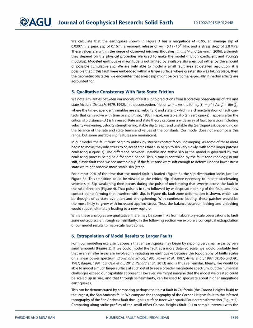
Additionally, not only are faults self-similar but the earthquakes that occuron them are shown to have self-similarslip distributions. Manighetti et al.[2005] examined more than 100global earthquake slip distributionsand found that they are asymmetric,being dominated by one region ofstrong slip followed by a long-tailedgradient that they describe as triangu-lar in shape (Figure 8). They demon-strate that the high-slip patches(asperities) occupy approximatelyone third of the slip area and thathigh-slip patches are structurallybound by intersections or a changein strike. We note that the slip profilesfrom our simulated earthquakes havethis characteristic (Figure 8), whichlends some support for extrapolatingrupture processes modeled at scalesbetween 10�1 and 102m upward to

larger faults. To the degree that our model represents an actual earthquake, then the high-slip region withgreatest relief (Figure 4) might be an image of an asperity.

7. Conclusions

A numerical model taken directly from a measured natural fault surface can spontaneously generate stick-slipearthquake behavior. Initiation and termination of slip are controlled by stress heterogeneity that is in turn gov-erned by changing contact geometry as slip evolves. Slip initiates in areas of strong surface gradients, wheresmall displacements locally unclamp the fault. Slip terminates when multiple sticking points evolve where othersteep gradient points collide (increased clamping stress). We show that the fault surface must change shapebefore slip can occur again and suggest that maturing faults must constantly change shape over time. Eitherthese geometrical slip barriers smooth out as a fault system lengthens, leading to characteristic, larger-magnitudeearthquakes, or self-similarity may lead to magnitude dependent segmentation. Post-rupture juxtaposition ofnew contacts and rupture barriers may make exact earthquake repeats rare except on very smooth faults.

ReferencesAki, K. (1987), Magnitude-frequency relation for small earthquakes: A clue to the origin of fmax of large earthquakes, J. Geophys. Res., 92,

1349–1355, doi:10.1029/JB092iB02p01349.Aviles, C. A., C. H. Scholz, and J. Boatwright (1987), Fractal analysis applied to characteristic segments of the San Andreas fault, J. Geophys.

Res., 92, 331–344, doi:10.1029/JB092iB01p00331.Ben-David, O., and J. Fineberg (2011), Static friction coefficient is not a material constant, Phys. Rev. Lett., 106, 254301.Bevk, A. (2013), Curbed SF. [Available at http://sf.curbed.com/archives/2013/08/12/rock_blasting_and_brick_making_atop_corona_

heights_park.php.]Brown, S. R., and C. H. Scholz (1985), Broad bandwidth study of the topography of natural rock surfaces, J. Geophys. Res., 90, 12,575–12,582,

doi:10.1029/JB090iB14p12575.Candela, T., F. Renard, J. Schmittbuhl, M. Bouchon, and E. E. Brodsky (2011), Fault slip distribution and fault roughness, Geophys. J. Int., 187,

959–968, doi:10.1111/j.1365-246X.2011.05189.x.Candela, T., F. Renard, Y. Klinger, K. Mair, J. Schmittbuhl, and E. E. Brodsky (2012), Roughness of fault surfaces over nine decades of length

scales, J. Geophys. Res., 117, B08409, doi:10.1029/2011JB009041.Childs, C., T. Manzocchi, J. J. Walsh, C. G. Bonson, A. Nicol, and M. P. J. Schöpfer (2009), A geometric model of fault zone and fault rock

thickness variations, J. Struct. Geol., 31(2), 117–127.Collettini, C., A. Niemeijer, C. Viti, and C. Marone (2009), Fault zone fabric and fault weakness, Nature, 462, 907–910.Coon, E. T., B. E. Shaw, and M. Spiegelman (2011), A Nitsche-extended finite element method for earthquake rupture on complex fault

systems, Comput. Methods Appl. Mech. Eng., 200(41–44), 2859–2870.Dieterich, J. H. (1979), Modeling of rock friction: 1. Experimental results and constitutive equations, J. Geophys. Res., 84, 2161–2168,

doi:10.1029/JB084iB05p02161.Dieterich, J. H. (1992), Earthquake nucleation on faults with rate-and state-dependent strength, Tectonophysics, 211, 115–134.

Figure 8. Blue lines show example slip versus distance profiles as modeledalong the Corona Heights fault (axis labels refer to these lines). Gray linesshow normalized examples from Manighetti et al. [2005] from measuredsurface slip along strike of globalM = 6.3–M = 7.7 earthquakes. The purposeof this figure is to show that simulated and observed earthquakes havecomparable, asymmetric slip distributions.

Journal of Geophysical Research: Solid Earth 10.1002/2015JB012448

PARSONS AND MINASIAN NUMERICAL FAULT MODEL FROM LIDAR 7861

AcknowledgmentsWe thank Chris Marone, an anonymousreviewer, and Editor Bob Nowack fortheir helpful comments and suggestionson this manuscript. Data are freelyavailable from the authors.

Duan, B., and D. D. Oglesby (2005), The dynamics of thrust and normal faults over multiple earthquake cycles: effects of dipping faultgeometry, Bull. Seismol. Soc. Am., 95, 1623–1636, doi:10.1785/0120040234.

Faulkner, D. R., T. M. Mitchell, E. H. Rutter, and J. Cembrano (2008), On the structure and mechanical properties of large strike-slip faults,Geol. Soc. Spec. Publ., 299, 139–150.

Field, E. H., and M. T. Page (2011), Estimating earthquake-rupture rates on a fault or fault system, Bull. Seismol. Soc. Am., 101, 79–92,doi:10.1785/0120100004.

Field, E. H., et al. (2014), Uniform California Earthquake Rupture Forecast, Version 3 (UCERF3)—The time-independent model, Bull. Seismol.Soc. Am., 104, 1122–1180, doi:10.1785/0120130164.

Fournier, T., and J. Morgan (2012), Insights to slip behavior on rough faults using discrete element modeling, Geophys. Res. Lett., 39, L12304,doi:10.1029/2012GL051899.

Gudmundsson, A. (2004), Effects of Young’s modulus on fault displacement, C. R. Geosci., 336, 85–92.Imanishi, K., and W. L. Ellsworth (2006), Source scaling relationships of microearthquakes at Parkfield, CA, determined using the SAFOD pilot

hole seismic array, in Earthquakes: Radiated Energy and the Physics of Faulting, edited by R. Abercrombie et al., AGU, Washington, D. C.,doi:10.1029/170GM10.

Jennings, C. W. (1994), Fault activity map of California and adjacent areas with locations and ages of recent volcanic eruptions, CaliforniaDivision of Mines and Geology Data Map Series No. 6, 92 p., 2 plates, map scale 1:750,000.

Kagan, Y. Y. F. (1991), Dimension of brittle fracture, J. Nonlinear Sci., 1, 1–16.Kezdi, A. (1974), Handbook of Soil Mechanics, 294 pp., Elsevier, Amsterdam.Kirkpatrick, J. D., and E. E. Brodsky (2014), Slickenline orientations as a record of fault rock rheology, Earth Planet. Sci. Lett., 408, 24–34,

doi:10.1016/j.epsl.2014.09.040.Kirkpatrick, J. D., C. D. Rowe, J. C. White, and E. E. Brodsky (2013), Silica gel formation during fault slip: Evidence from the rock record, Geology,

41, 1015–1018, doi:10.1130/G34483.1.Lockner, D. A., and J. D. Byerlee (1993), How geometrical constraints contribute to the weakness of mature faults, Nature, 363, 250–252.Lynch, J. C., and M. A. Richards (2001), Finite element models of stress orientations in well-developed strike-slip fault zones: Implications for

the distribution of lower crustal strain, J. Geophys. Res., 106, 26,707–26,729, doi:10.1029/2001JB000289.Main, I. (1996), Statistical physics, seismogenesis, and seismic hazard, Rev. Geophys., 34, 433–462, doi:10.1029/96RG02808.Manighetti, I., M. Campillo, C. Sammis, P. M. Mai, and G. King (2005), Evidence for self-similar, triangular slip distributions on earthquakes:

Implications for earthquake and fault mechanics, J. Geophys. Res., 110, B05302, doi:10.1029/2004JB003174.Marone, C. (1995), Fault zone strength and failure criteria, Geophys. Res. Lett., 22, 723–726, doi:10.1029/95GL00268.Marone, C., and B. Kilgore (1993), Scaling of the critical slip distance for seismic faulting with shear strain in fault zones, Nature, 362, 618–621.Marone, C., M. Cocco, E. Richardson, and E. Tinti (2009), The critical slip distance for seismic and aseismic fault zones of finite width, Int. Geophys.,

94(C), 135–162.Moore, D. E., and M. J. Rymer (2007), Talc-bearing serpentinite and the creeping section of the San Andreas fault, Nature, 448, 795–797.Murchey, B. L., and D. L. Jones (1984), Age and significance of chert in the Franciscan Complex in the San Francisco Bay Region, in Franciscan

Geology of Northern California, vol. 43, edited by M. C. Blake Jr., pp. 23–30, Pacific Section S.E.P.M.Noda, H., E. M. Dunham, and J. R. Rice (2009), Earthquake ruptures with thermal weakening and the operation of major faults at low overall

stress levels, J. Geophys. Res., 114, B07302, doi:10.1029/2008JB006143.Okubo, P. G., and K. Aki (1987), Fractal geometry in the San Andreas fault system, J. Geophys. Res., 92, 345–355, doi:10.1029/JB092iB01p00345.Page, M., and K. Felzer (2015), Southern San Andreas fault seismicity is consistent with the Gutenberg-Richter magnitude-frequency

distribution, Bull. Seismol. Soc. Am., 105, doi:10.1785/0120140340.Page, M. T., D. Alderson, and J. Doyle (2011), The magnitude distribution of earthquakes near Southern California faults, J. Geophys. Res., 116,

B12309, doi:10.1029/2010JB007933.Power, W. L., and T. E. Tullis (1992), The contact between opposing fault surfaces at Dixie Valley, Nevada, and implications for fault

mechanics, J. Geophys. Res., 97, 15,425–15,435, doi:10.1029/92JB01059.Power, W. L., T. E. Tullis, S. Brown, G. N. Boitnott, and C. H. Scholz (1987), Roughness of natural fault surfaces, Geophys. Res. Lett., 14, 29–32,

doi:10.1029/GL014i001p00029.Renard, F., T. Candela, and E. Bouchaud (2013), Constant dimensionality of fault roughness from the scale of micro-fractures to the scale of

continents, Geophys. Res. Lett., 40, 83–87, doi:10.1029/2012GL054143.Rice, J. R. (1992), Fault stress states, pore pressure distributions, and the weakness of the San Andreas Fault, in Fault Mechanics and Transport

Properties of Rocks; A Festschrift in Honor of W. F. Brace, edited by B. Evans and T. Wong, pp. 475–503, Acad. Press, San Diego, Calif.Ruina, A. (1983), Slip instability and state variable friction laws, J. Geophys. Res., 88, 10,359–10,370, doi:10.1029/JB088iB12p10359.Sagy, A., E. E. Brodsky, and G. J. Axen (2007), Evolution of fault-surface roughness with slip, Geology, 35, 283–286.Schlocker, J. (1974), Geology of the San Francisco North quadrangle, California, U.S. Geol. Surv. Prof. Pap., 782, 109.Scholz, C. H. (1987), Wear and gouge formation in brittle faulting, Geology, 15, 493–495.Scholz, C. H. (2002), The Mechanics of Earthquake Faulting, Cambridge Univ. Press, Cambridge, U. K.Schwartz, D. P., and K. J. Coppersmith (1984), Fault behavior and characteristic earthquakes: examples from the Wasatch and San Andreas

fault zones, J. Geophys. Res., 89, 5681–5698, doi:10.1029/JB089iB07p05681.Sibson, R. H. (2003), Thickness of the seismic slip zone, Bull. Seismol. Soc. Am., 93, 1169–1178.Stein, S., and A. Newman (2004), Characteristic and uncharacteristic earthquakes as possible artifacts: Applications to the New Madrid and

Wabash seismic zones, Seismol. Res. Lett., 75, 173–187.Toppozada, T. R., D. M. Branum, M. S. Reichle, and C. L. Hallstrom (2002), San Andreas fault zone, California: M ≥5.5 earthquake history,

Bull. Seismol. Soc. Am., 92, 2555–2601.Wells, D. L., and K. J. Coppersmith (1994), New empirical relationships among magnitude, rupture length, rupture width, rupture area, and

surface displacement, Bull. Seismol. Soc. Am., 84, 974–1002.Wesnousky, S. G. (1994), The Gutenberg-Richter or characteristic earthquake distribution, which is it?, Bull. Seismol. Soc. Am., 84, 1940–1959.Wesnousky, S. G. (2006), Predicting the endpoints of earthquake ruptures, Nature, 444, 358–360.Wibberley, C. A. J., G. Yielding, and G. Di Toro (2008), Recent advances in the understanding of fault zone internal structure: A review,

Geol. Soc. Spec. Publ., 299, 5–33.Xing, H. L., P. Mora, and A. Makinouchi (2004), Finite element analysis of fault bend influence on stick–slip instability along an intra-plate fault,

Pure Appl. Geophys., 161, 2091–2102, doi:10.1007/s00024-004-2550-1.Xu, S., E. Fukuyama, Y. Ben-Zion, and J.-P. Ampuero (2015), Dynamic rupture activation of backthrust fault branching, Tectonophysics,

644–645, 161–183.

Journal of Geophysical Research: Solid Earth 10.1002/2015JB012448

PARSONS AND MINASIAN NUMERICAL FAULT MODEL FROM LIDAR 7862