Earth and Planetary Science Letters 415 (2015) 134–141

Contents lists available at ScienceDirect

Earth and Planetary Science Letters

www.elsevier.com/locate/epsl

Accelerated West Antarctic ice mass loss continues to outpace East Antarctic gains

Christopher Harig ∗, Frederik J. Simons

Department of Geosciences, Princeton University, Princeton, NJ, USA

a r t i c l e i n f o a b s t r a c t

Article history:Received 23 June 2014Received in revised form 22 January 2015Accepted 24 January 2015Available online xxxxEditor: Y. Ricard

Keywords:

climate

Antarctica

satellite measurements

time-variable gravity

While multiple data sources have confirmed that Antarctica is losing ice at an accelerating rate, different measurement techniques estimate the details of its geographically highly variable mass balance with different levels of accuracy, spatio-temporal resolution, and coverage. Some scope remains for methodological improvements using a single data type. In this study we report our progress in increasing the accuracy and spatial resolution of time-variable gravimetry from the Gravity Recovery and Climate Experiment (GRACE). We determine the geographic pattern of ice mass change in Antarctica between January 2003 and June 2014, accounting for glacio-isostatic adjustment (GIA) using the IJ05_R2 model. Expressing the unknown signal in a sparse Slepian basis constructed by optimization to prevent leakage out of the regions of interest, we use robust signal processing and statistical estimation methods. Applying those to the latest time series of monthly GRACE solutions we map Antarctica’s mass loss in space and time as well as can be recovered from satellite gravity alone. Ignoring GIA model uncertainty, over the period 2003–2014, West Antarctica has been losing ice mass at a rate of −121 ± 8 Gt/yr and has experienced large acceleration of ice mass losses along the Amundsen Sea coast of −18 ± 5 Gt/yr2, doubling the mass loss rate in the past six years. The Antarctic Peninsula shows slightly accelerating ice mass loss, with larger accelerated losses in the southern half of the Peninsula. Ice mass gains due to snowfall in Dronning Maud Land have continued to add about half the amount of West Antarctica’s loss back onto the continent over the last decade. We estimate the overall mass losses from Antarctica since January 2003 at −92 ± 10 Gt/yr.

2015 Elsevier B.V. All rights reserved.

1. Introduction

Knowing where and how mass currently changes in polar ice sheets is of great importance (Oppenheimer, 1998; Mitrovica et al., 2011; Stocker et al., 2013). Observations indicate that the Antarctic Ice Sheet is very sensitive to climate change (Raymo and Mitrovica, 2012; Bromwich et al., 2013; Cook et al., 2013;Kopp et al., 2013), and knowledge of individual glaciers and ice streams is important to understand the process. Ultimately, the continental ice sheet response to global change is the sum of the behaviors within individual drainage basins, which are subject to the combined effects of surface mass balance, calving and basal melting, and influenced by their geographic location and topog-raphy. The contemporary record of ice sheet mass balance has solidified significantly partly owing to the data gathered since 2002 by GRACE, the Gravity Recovery and Climate Experiment (Chen

* Corresponding author.E-mail address: charig@princeton.edu (C. Harig).

et al., 2006, 2009; Velicogna and Wahr, 2006). The continent-wide, decadally averaged mass balances of Antarctica, estimated by a variety of techniques, all show that Antarctica is losing mass (Shepherd et al., 2012; Hanna et al., 2013) at an accelerated rate (Luthcke et al., 2013; Williams et al., 2014).

While the large-scale spatial and long-term temporal signal trends during the 1990s and 2000s have been well determined, we focus here on the smaller scales recoverable by satellite grav-ity, and quantify their uncertainty. In Antarctica, improvements in modeling the ongoing glacio-isostatic adjustment from the Last Glacial Maximum deglaciation (for an accessible review, see King, 2013) have increased the precision of gravimetric mass balance estimates. As a result, the detailed pattern of mass change has been the focus of recent GRACE studies (Sasgen et al., 2010, 2013; Harig and Simons, 2012; Horwath et al., 2012; King et al., 2012;Lee et al., 2012; Luthcke et al., 2013; Velicogna and Wahr, 2013;Bouman et al., 2014). To inform our estimates of sea level change for the coming century it is imperative that we continue to build and improve the detailed record of changes in ice mass (Overpeck et al., 2006; Little et al., 2013a, 2013b). In this paper we show

http://dx.doi.org/10.1016/j.epsl.2015.01.029

0012-821X/ 2015 Elsevier B.V. All rights reserved.

C. Harig, F.J. Simons / Earth and Planetary Science Letters 415 (2015) 134–141 135

when and where Antarctica has been losing mass over the last decade, using a method of spherical Slepian functions.

2. Motivation

As GRACE processing of intersatellite range-rates (Rowlands et al., 2005; Luthcke et al., 2006; Bettadpur and the CSR Level-2 Team, 2012) and global statistical estimation techniques (Schmidt et al., 2006; Han et al., 2008; Baur et al., 2009; Rowlands et al., 2010) have improved in recent years, the opportunity for con-temporary gravimetric studies is to produce a better-resolved ice mass history and to understand its error structure at the same time. Knowledge of ice mass balance at a fine level of spatial de-tail is ultimately required to enable comparisons of gravity-based estimates with other data sets and models that discretely sam-

ple the surface. Data sets and models from point estimates (e.g., laser and radar altimetric observations, GPS time series, or sur-face mass balance studies) show that Antarctica’s mass flux is highly spatially variable (Rignot et al., 2008a; Lenaerts et al., 2012;Pritchard et al., 2012). Fast-moving glaciers along the Amundsen Sea coast contribute the greatest amount of mass loss (Rignot, 2008; Rignot et al., 2011; Pritchard et al., 2009), while areas of the Antarctic Peninsula (Rignot et al., 2004) and Wilkes Land (Rignot et al., 2008a) are estimated to have experienced more modest losses. These high-resolution non-gravimetric observations are substanti-ated by our own new gravity-based results, which are aggregate, not point-based, measurements. The subtle differences between our regional solutions and those of other authors suggest that re-fining analysis approaches, increasing spatial resolution, and noise mitigation will all remain important research topics in the near fu-ture.

Rather than building a consensus model from different data types, each mismatched in their footprint and individual sensitivi-ties to ice mass changes, here we use a uniquely sensitive Slepian-function based gravimetric processing method to localize global GRACE data to several Antarctic regions that display distinct ge-ographic variability, and subsequently focus on the map changes over time within each region. In the main body of this paper we focus our attention on results obtained for the regions of greatest mass change in West Antarctica, and discuss ice mass loss trends in the Peninsula and Dronning Maud Land. Additional details are examined in the Supplementary Material.

3. Methods

In this study we use time-variable gravimetry to determine the mass change in Antarctica since 2003. We closely follow the methods of Harig and Simons (2012) and analyze GRACE Level 2 data using scalar spherical Slepian functions (Simons et al., 2006). GRACE data are released as coefficients to spherical harmonic func-tions, which spread their energy over the entire globe. In order to examine geophysical signals in specific regions, most authors (ourselves included) project global gravity data into alternate re-gionally sensitive bases, such as wavelets or radial basis functions (Schmidt et al., 2007; Eicker et al., 2014), pixel grids (Chen et al., 2009), point masses or mascons expressed as sensitivity functions in spherical harmonics (Baur and Sneeuw, 2011; Jacob et al., 2012;Luthcke et al., 2013; Schrama et al., 2014). Many of these ap-proaches suffer the same limitations as spherical harmonics when used for regional analysis, namely a lack of orthogonality over ar-bitrary regions of interest. As a result, these approaches often use regularized inversion procedures which can sometimes negatively impact results (e.g., Bonin and Chambers, 2013). Spherical Slepian functions, by construction, are orthogonal both over the globe and over individual regions, thus simplifying data analysis.

3.1. Construction of the Slepian basis

The Slepian basis is a spatiospectrally localized linear combina-

tion of spherical harmonics optimized to study specific regions on the sphere (for a review, see Simons, 2010). The simplicity of the Slepian basis method is that its construction is tuned by only three variables: the spherical-harmonic bandwidth of the basis, the co-ordinates of the spatial region under study, and any buffer around the outlines of the region proper, to account for possible mass changes near the edges. The triplet of parameters is picked after a sequence of simulations using synthetic input data.

Our initial coordinate outlines for the Antarctic regions include grounded ice (except for the Peninsula, where all floating ice was used, as noted below and in the Supplementary Material) deter-mined from ICESat altimetry (Zwally et al., 2012). Those regions were then enlarged with a buffer of 0.5 extending outward from land–ocean borders. The size of the buffer zone was determined by simulating and recovering a uniform mass change over grounded ice, to render the overall mass estimate unbiased. The buffer ac-counts for the fact that smoothly varying bandlimited functions are ill-suited for recovering a field near to a region boundary. The bandwidth of the Slepian bases covers spherical-harmonic de-grees up to L = 60, which matches the bandwidth of GRACE data supplied by most data centers. Thus there is no loss of spatial res-olution by projecting the Level 2 data onto the Slepian bases.

We use the outline of the region R to integrate the products of spherical harmonics Y lm as∫

R

Y lmY l′m′ dΩ = Dlm,l′m′ . (1)

The spherical-harmonic expansion coefficients of the Slepian functions, glm , are the eigensolutions of the equation

L∑l′=0

l′∑m′=−l′

Dlm,l′m′ gl′m′ = λglm. (2)

The functions maximize their energy within the specified re-gion; the corresponding eigenvalue λ is a measure of that con-centration (Simons et al., 2006). Using only the most concentrated eigenfunctions (λ 0.5) leaves a low-dimensional scalar Slepian basis for the inverse problem, similar to a singular-value decompo-

sition, which we can use to represent the potential field localized to our region without undue influence from other parts of the globe. In this manner, we explicitly seek to minimize the leakage in and out of our region. Truncated expansions of Slepian functions have many advantages over damped spherical-harmonic expres-sions for these kinds of estimation problems (Simons and Dahlen, 2006).

3.2. Solution of the inverse problem

With a sparse representation of the signal (which is perhaps the greatest advantage of the Slepian-function approach, and one that is successfully exported to inverse problems in other areas of geophysics and planetary studies; Simons et al., 2009) and em-

pirical knowledge of the noise distribution (as derived from the correlation structure of the misfit of the expansion coefficients with respect to the modeled temporal behavior) our procedure extracts the time-variable geographic mass distribution with a unique spatio-temporal resolution. By increasing the local signal-to-noise ratio, the Slepian basis remains sensitive to spatial fea-tures within the region at the full resolution of the Level 2 GRACE data (up to a spherical-harmonic degree L = 60; higher-bandwidth solutions, up to L = 90, exist, but suffer from decreased signal-to-noise ratios), and we become less reliant on the spatial averaging

136 C. Harig, F.J. Simons / Earth and Planetary Science Letters 415 (2015) 134–141

methods (e.g., by Gaussian smoothing prior to analysis) employed by most other authors. In the case of Greenland, these benefits allowed high-significance detections of accelerations in the mass loss, and better constrained location and timing of these changes (Harig and Simons, 2012).

When the monthly GRACE gravity fields are projected into a new basis for a specific region, the spherical-harmonic coefficients are transformed into Slepian coefficients, one per month for each basis function. Since the basis functions are orthogonal over the region under consideration, we may invert the coefficient time se-ries individually for the least-squares-error estimates of temporal trends within the region. We solve for a temporal model with sea-sonal (182.5 day) and annual (365 day) Fourier terms, and a first, second, or third-order polynomial in time, as warranted by signifi-cance tests. We refrain from fitting a 161 day S2 tidal alias (or any other tidal aliasing term). When it is included the amplitudes of the other two periodic functions are altered, but parameters of the polynomial functions (our trends and accelerations) are not signif-icantly changed (even though it reduces their uncertainties).

We form spatial maps of mass changes by re-expanding the best-fitting (predicted) coefficients for each Slepian function into the space domain and summing them. We furthermore estimate the temporal trend of the total mass change by expanding the orig-inal Slepian coefficients into space, integrating over the region, and inverting for the trend exhibited by their sum.

While each GRACE monthly solution is treated independently, their time series exhibits temporal autocorrelation of the residu-als after fitting, owing to various unmodeled signals. Compared to our earlier work, we now use a generalized least-squares proce-dure which iteratively solves for the full covariance model of het-eroscedasticity and autocorrelation in the presence of an AR(1) au-

toregressive noise process, as suggested by Williams et al. (2014), implemented using Matlab’s fgls. This results, in some cases, in confidence bounds that are up to 50% larger than with ordinary least-squares. All of our uncertainties are obtained using this new methodology, and are presented at the two sigma level.

3.3. Assessing spatial resolution

It is difficult to compare spatial resolution between model-

ing approaches without detailed considerations to quantify bias, variance, signal-to-noise ratios, and the effect of bandwidth selec-tion (Simons and Dahlen, 2006; Slobbe et al., 2012). Nevertheless, a detailed comparative study by Longuevergne et al. (2010), car-ried out on the scale of hydrological basins, independently of our own efforts, was indicative of favorable behavior of the approaches based on Slepian functions. Since we never abandon the L = 60

bandwidth of the Level 2 products, the equivalent ∼330 km half-wavelength is our nominal spatial resolution. The number of terms in the Slepian expansion, the degrees of the temporal polynomial functions, and the size of the buffer zone around the primary re-gions of interest were determined by synthetic modeling focused on removing leakage effects and obtaining nearly unbiased esti-mates for regionally averaged mass loss signals.

The effort in constructing the Slepian functions is minimal, as they are efficiently computed via variety of numerical meth-

ods, both on the sphere (Simons and Dahlen, 2007) and in the plane (Simons and Wang, 2011). Compared to other gravity-

based approaches, we do not a priori remove correlations be-tween spherical-harmonic coefficients (Swenson and Wahr, 2006), and neither smooth nor project on a predefined basin structure (Wouters et al., 2008; King et al., 2012; Sasgen et al., 2012, 2013). Rather, we determine full-resolution best-localized scalar Slepian basis sets for large regions encompassing several basins; we project the GRACE Level 2 coefficients onto well-concentrated trun-cated subsets of each basis; and then we estimate the correlation

structure of the residuals as part of the estimation of the spatio-temporal behavior of the Slepian coefficient time series.

4. Data and models

We used 129 monthly GRACE Release 5 geopotential fields from the Center for Space Research (CSR RL-05 in our labeling), Univer-sity of Texas at Austin, covering the longest GRACE time span to date, from January 2003 to June 2014, including nine months with data gaps. These solutions include the October 2014 reprocessing which corrected errors in the atmosphere–ocean model (AOD1B) used to create GRACE Level 2 data, affecting monthly solutions from June 2013 onward. Degree-two order-zero spherical-harmonic coefficients were replaced with those determined from satellite laser ranging (Cheng et al., 2013). Degree-one coefficients for the geocenter motion were included as calculated by Swenson et al.(2008). For those, values from satellite laser ranging would be an alternative; the influence of different choices on the final results has been compared in detail (e.g., Schrama et al., 2014). Uncer-tainty estimates for these two coefficient corrections are not in-cluded in our reported values. We transformed the geopotential fields into surface mass density by removing the gravitational ef-fect of instantaneous elastic deformation arising from current mass change (le Meur and Huybrechts, 1996), in a Love number loading formalism (Wahr et al., 1998). We did not correct for the bias of migrating water that accompanies changes in ice mass (Sterenborg et al., 2013), nor did we account for the influence of recent sea level rise trends in the Southern Ocean (Rye et al., 2014) on our estimation. Global surface mass density fields were projected into a Slepian basis specifically designed for the regions of interest, such as all of Antarctica, its regions West Antarctica, the Penin-sula, Dronning Maud and Wilkes Lands, and so on.

We corrected for the ongoing solid Earth deformation from prior changes in ice load by subtracting a glacio-isostatic adjust-ment (GIA) model projected onto the same basis. We report results using two recent GIA models, both also used by Shepherd et al.(2012): the IJ05_R2 (Ivins et al., 2013) model (in the Main Text) and the W12a_v1 model (Whitehouse et al., 2012) in the Supple-mentary Material. The IJ05_R2 model used is the best case for litho-sphere thickness h = 65 km with upper-mantle and lower-mantle viscosities of ηUM = 2 ×1020 Pa s and ηLM = 1.5 ×1021 Pa s, respec-tively. The W12a_v1 model ‘B’ (best) was used, corresponding to lithospheric thickness h = 120 km, upper-mantle viscosity ηUM =

1 ×1021 Pa s, and lower-mantle viscosity ηLM = 10 ×1022 Pa s. Cor-rections for GIA primarily alter the slope of mass change and, to some extent, the average map pattern of mass change. However, they do not alter non-linear changes such as accelerations. We do not include the uncertainty of the GIA models as part of the un-certainty in our ice mass estimates, but rather report the results of our analysis after using one or the other GIA model, both ge-ographically variable in different ways. Trend estimates bracketed by the full range of GIA models can be found in the Supplementary Material.

5. Results and discussion

5.1. Continent-wide ice mass loss

Fig. 1, the map of the total ice mass change modeled from the CSR solutions between January 2003 and June 2014, shows the overall pattern of mass change over the whole of Antarc-tica. Our map was produced with a Slepian basis localized over the (buffered) portion of Antarctica that includes grounded ice, and the patterns of mass loss retrieved suggested subregions for closer inspection. Antarctica’s surface area warrants the use of just 100 Slepian basis functions, a favorable reduction of the degrees

C. Harig, F.J. Simons / Earth and Planetary Science Letters 415 (2015) 134–141 137

Fig. 1. Ice mass change (mass corrected using the GIA model by Ivins et al., 2013) over Antarctica for the period January 2003 to June 2014. This solution is from a localization over the whole of Antarctica. Solid black line is a rough coastline includ-ing ice fronts. Dashed line is our localization region outline which is a 0.5 buffered version of grounded ice determined from altimetry (all ice fronts were used for the Peninsula, see Supplementary Material). The integral value (Int = −925) is the total change for the entire epoch, in gigatons (Gt). Regional solutions for West Antarctica, the Antarctic Peninsula, and Dronning Maud Land, are shown in Fig. 3 (covering the areas of box a and box b) and in the Supplementary Material (for box c), respectively.

of freedom in the estimation problem by 97.3% per cent for the spherical-harmonic bandwidth of L = 60 (which would otherwise require the estimation of 3721 spherical-harmonic expansion co-efficients prior to smoothing and basin projection). Repeating our analysis (see Supplementary Material) for the RL-05a solutions pro-vided by the GeoForschungsZentrum (GFZ), over the same time interval, at the same bandwidth of L = 60 (Dahle et al., 2013), and using the same GIA correction model (IJ05_R2), yields spa-tial patterns very similar to those of our solutions shown in Fig. 1. The continent-wide total change obtained from the CSR solutions is slightly lower than that from the GFZ solutions (−925 Gt vs. −1016 Gt ice mass loss, January 2003 to June 2014), but using the GFZ solutions leads to slightly more spatial variability (Fig. S4).

The continent-wide Antarctic pattern of mass change agrees generally well with that recovered by previous studies (Chen et al., 2008, 2009; Horwath et al., 2012; King et al., 2012; Shepherd et al., 2012; Luthcke et al., 2013; Velicogna and Wahr, 2013). Our in-dividual inversions for the trends displayed by smaller subregions reveals that West Antarctica (Fig. 1, box a) has experienced the largest-magnitude mass changes. The areas of greatest mass loss are centered around the Thwaites Glacier area of the Amundsen Sea Coast. Mass gains are also observed near the Kamb Ice Stream (Shepherd et al., 2012), associated with long-term thickening and reduced ice stream flow velocities (Joughin and Tulaczyk, 2002; Pritchard et al., 2012, 2009). Areas of Wilkes and Victoria Land (∼150–115E) show more moderate amounts of mass loss (Chen et al., 2009). The Antarctic Peninsula (Fig. 1, box b) also shows moderate mass loss, the details of which are geographically dis-tinct and are discussed further below. Finally, Dronning Maud Land in East Antarctica (∼0–45E; Fig. 1, box c) has been gaining mass, the majority of which since 2009 (see Supplementary Material).

5.2. Regional ice mass loss: temporal trends

The residual (i.e. unmodeled) behaviors of the ice mass flux over broad regions within Antarctica are generally uncorrelated in

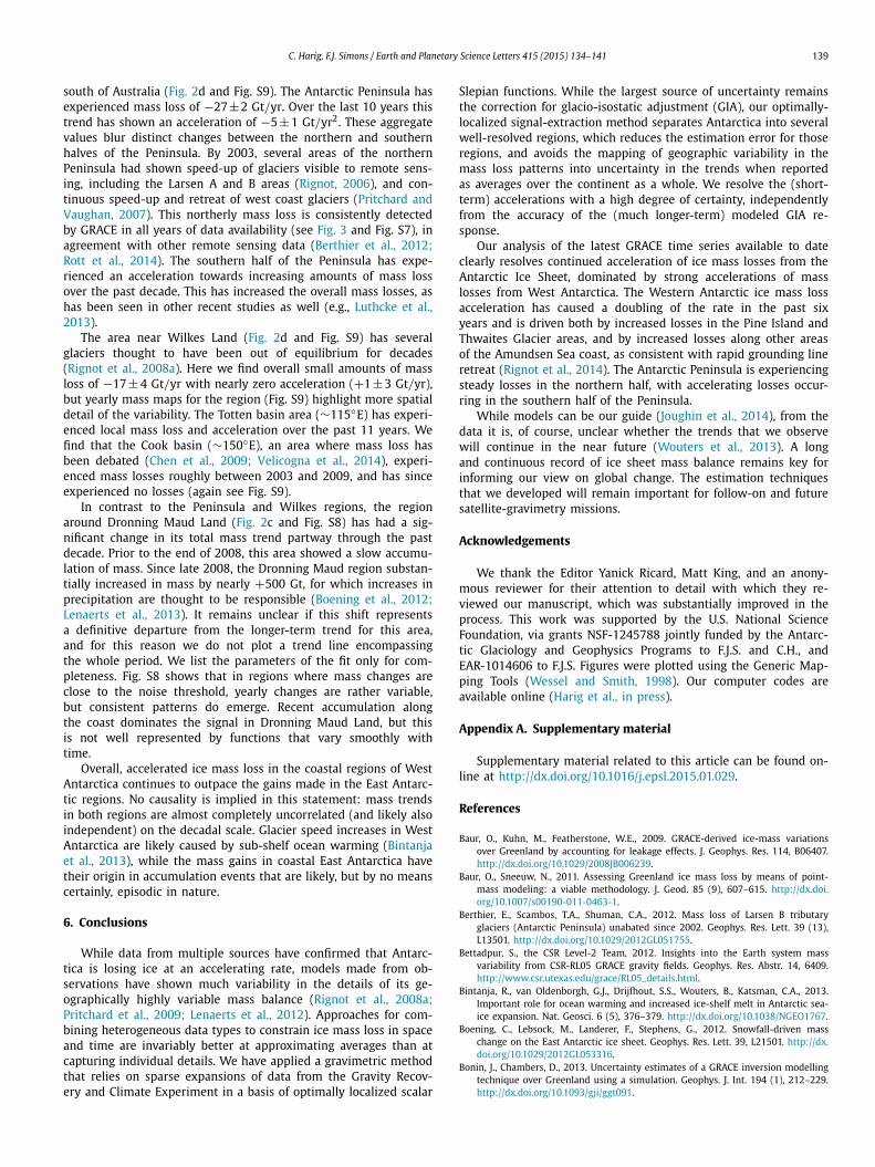
Fig. 2. Ice mass changes (mass corrected using the GIA model by Ivins et al., 2013) in gigatons (Gt) for several regions of Antarctica including West Antarctica, the Antarctic Peninsula, Dronning Maud Land, Wilkes Land, and the whole of Antarc-tica. The regions covered by each localization are shaded red in the top right inset. The black lines are monthly GRACE observations with 2σ error bars determined from our analysis. The solid blue lines are the best-fit quadratic curves. We elect not to plot a trend line in panel c, listing the parameters of the fit only for com-

pleteness.

our model. However, the geographical (i.e. spatial) variability at the basin scale does not necessarily average out at the larger scales, but can map into increased variance of the mean behavior. This causes the average ice loss over the continent to be less precisely estimated than the averages over individual regions. To observe more local changes, and to make the errors on the mean behav-ior more representative of the estimation uncertainty that can be achieved over regions that behave more coherently in time, we used the continent-wide solution (Fig. 1) as a guide to further lo-calize five individual regions of Antarctica. Hints of more detailed interannual variations observed by others (Horwath et al., 2012)in these five regions can be seen as deviations from the trends in our plots of the total mass (Fig. 2). However, our regions are con-servatively chosen and thus too large to adequately characterize the complex temporal variations that might differentiate individ-ual Antarctic basins from the gravity data alone.

138 C. Harig, F.J. Simons / Earth and Planetary Science Letters 415 (2015) 134–141

Upon spatial integration and summation of the Slepian basis functions and their corresponding coefficients we produce time se-ries for the total mass of each region (Fig. 2). The ice mass trends estimated from the monthly observations strongly depend on the time window of the data analyzed, on the specific GIA model used to correct the data, and on the chosen corrections for degree-two and degree-one spherical-harmonic terms. Here, we note that our trend obtained from the localization to all of Antarctica simulta-

neously (Fig. 2e) agrees within error with the results reported by Shepherd et al. (2012) for their same temporal observation win-

dows, specifically the GRACE-only solutions covering January 2003 to December 2010 and October 2003 to December 2008. The lat-ter study combined results across measurement techniques and by many authors, including many GRACE groups.

We find the total mass trend for all of Antarctica from January 2003 to June 2014 to be −92 ±10 Gt/yr. The total mass change ac-celeration over the period 2003–2014 is −6 ± 6 Gt/yr2 . The trend value is within error of other recent studies (Luthcke et al., 2013;Sasgen et al., 2013; Velicogna and Wahr, 2013). Beyond differences in the purely statistical treatment of the data, the choice of degree-one coefficients used in the correction for geocenter-motion will be partly responsible for disagreement between studies. Our reported acceleration for the whole continent is somewhat lower than other recent results, as the past 18 months of data have lowered earlier acceleration estimates.

The total ice mass curves for the smaller regions within Antarc-tica clearly show strong interregional variations. West Antarctica (Fig. 2a) displays a large coherent trend of accelerating mass loss. The mean slope (−121 ± 8 Gt/yr) and acceleration (−18 ±5 Gt/yr2) are larger than in any other area of Antarctica (see also Joughin and Tulaczyk, 2002; Rignot et al., 2008a; Sasgen et al., 2013; Williams et al., 2014), and the variance of the observa-tions about this trend is much lower than that over the whole of Antarctica. Without the influence of variability in other re-gions, the estimation uncertainty for trends in West Antarctica (and other regions) is lower than for the whole continent. The accelerations are independent of any GIA effects (which operate on much longer time scales), and are consequently well deter-mined. Whether any such accelerations lie in the realm of nat-ural time-variability (Wouters et al., 2013; Williams et al., 2014)remains a separate question. While our continent-wide value is not larger than the decadal acceleration expected from stochastic climate-system variability over the whole continent, further study is needed to determine if this is also the case for West Antarctica alone, whose acceleration is much larger.

5.3. Regional ice mass loss: geographic patterns

We computed yearly-resolved ice mass change maps for each of the regions studied. Fig. 3 shows maps corresponding to the ag-gregate curves of Figs. 2a and 2b, and covers the areas of boxes a and b in Fig. 1. Each panel shows the ice mass changes from Jan-uary of the labeled year to January of the next, with units of cm/yr water equivalent surface density change. Changes seen between years in Fig. 3 thus correspond to accelerations, as linear changes would appear identical in the map pattern. As these maps are pro-duced from the coefficients fit over the entirety of the data time series, they cannot accurately reflect interannual variation shorter than about a few years.

For West Antarctica (see also Fig. 2a and Fig. S6), Fig. 3 shows how a small patch of ice mass loss near Pine Island and Thwaites Glaciers increases over the decade in intensity and in size, spread-ing over much of the Amundsen Sea coastal area. Peak values of the mass loss observed in places reach −50 cm/yr water equiv-alent. The intense acceleration of mass loss in the coastal areas has caused the total mass loss rate for West Antarctica to double

Fig. 3. Time-resolved maps of ice mass change (mass corrected using the GIA model by Ivins et al., 2013) over West Antarctica and the Antarctica Peninsula for odd years from 2003 to 2013. Each panel shows the estimated mass change from Jan-uary of the labeled year (e.g., 2003) to January of the following year (e.g., 2004). Changes seen between panels are due to accelerations. The top two rows of panels correspond to the area of box a in Fig. 1 and use the top scale bar. The bottom two rows use the bottom scale bar and correspond to box b in Fig. 1. For West Antarc-tica, the area of the localization includes grounded ice basins with a 0.5 buffer along ocean borders, and is outlined with a dashed line. For the Peninsula the lo-calization includes grounded ice and ice shelves with a 0.5 buffer, also shown with a dashed line. The integral values of the mass change per year are shown as “Int”, expressed in gigatons (Gt). When the color bar is saturated, as in 2011, the mini-

mum value of the field is shown in the top right as “Min” with units of centimeters per year water equivalent.

in the last six years. During the past decade steady low amounts of mass gain have been observed in the Kamb Ice Stream, as had been expected (Pritchard et al., 2012). The Pine Island and Thwaites Glacier areas have exhibited more negative mass balance since 1996 (Rignot et al., 2008a), due to either flow speed-ups, in Pine Island, or widening, over Thwaites (Rignot et al., 2008b). These changes have not yet been picked up by radar observa-tions of other glaciers along the Amundsen Sea coast (Rignot et al., 2008a). Ice shelves in this region lose a large portion of their mass via basal melting, implying a high sensitivity of the shelves (and hence grounded ice) to ocean warming (Rignot et al., 2013). Further monitoring is needed to detect these important changes in response to a changing climate.

We also examine regions for the Antarctic Peninsula (Fig. 2b and Fig. 3, and also Fig. S7), areas around Dronning Maud Land (Fig. 2c and Fig. S8), and areas near Wilkes and Victoria Lands

C. Harig, F.J. Simons / Earth and Planetary Science Letters 415 (2015) 134–141 139

south of Australia (Fig. 2d and Fig. S9). The Antarctic Peninsula has experienced mass loss of −27 ±2 Gt/yr. Over the last 10 years this trend has shown an acceleration of −5 ±1 Gt/yr2 . These aggregate values blur distinct changes between the northern and southern halves of the Peninsula. By 2003, several areas of the northern Peninsula had shown speed-up of glaciers visible to remote sens-ing, including the Larsen A and B areas (Rignot, 2006), and con-tinuous speed-up and retreat of west coast glaciers (Pritchard and Vaughan, 2007). This northerly mass loss is consistently detected by GRACE in all years of data availability (see Fig. 3 and Fig. S7), in agreement with other remote sensing data (Berthier et al., 2012;Rott et al., 2014). The southern half of the Peninsula has expe-rienced an acceleration towards increasing amounts of mass loss over the past decade. This has increased the overall mass losses, as has been seen in other recent studies as well (e.g., Luthcke et al., 2013).

The area near Wilkes Land (Fig. 2d and Fig. S9) has several glaciers thought to have been out of equilibrium for decades (Rignot et al., 2008a). Here we find overall small amounts of mass loss of −17 ±4 Gt/yr with nearly zero acceleration (+1 ±3 Gt/yr), but yearly mass maps for the region (Fig. S9) highlight more spatial detail of the variability. The Totten basin area (∼115E) has experi-enced local mass loss and acceleration over the past 11 years. We find that the Cook basin (∼150E), an area where mass loss has been debated (Chen et al., 2009; Velicogna et al., 2014), experi-enced mass losses roughly between 2003 and 2009, and has since experienced no losses (again see Fig. S9).

In contrast to the Peninsula and Wilkes regions, the region around Dronning Maud Land (Fig. 2c and Fig. S8) has had a sig-nificant change in its total mass trend partway through the past decade. Prior to the end of 2008, this area showed a slow accumu-

lation of mass. Since late 2008, the Dronning Maud region substan-tially increased in mass by nearly +500 Gt, for which increases in precipitation are thought to be responsible (Boening et al., 2012;Lenaerts et al., 2013). It remains unclear if this shift represents a definitive departure from the longer-term trend for this area, and for this reason we do not plot a trend line encompassing the whole period. We list the parameters of the fit only for com-

pleteness. Fig. S8 shows that in regions where mass changes are close to the noise threshold, yearly changes are rather variable, but consistent patterns do emerge. Recent accumulation along the coast dominates the signal in Dronning Maud Land, but this is not well represented by functions that vary smoothly with time.

Overall, accelerated ice mass loss in the coastal regions of West Antarctica continues to outpace the gains made in the East Antarc-tic regions. No causality is implied in this statement: mass trends in both regions are almost completely uncorrelated (and likely also independent) on the decadal scale. Glacier speed increases in West Antarctica are likely caused by sub-shelf ocean warming (Bintanja et al., 2013), while the mass gains in coastal East Antarctica have their origin in accumulation events that are likely, but by no means certainly, episodic in nature.

6. Conclusions

While data from multiple sources have confirmed that Antarc-tica is losing ice at an accelerating rate, models made from ob-servations have shown much variability in the details of its ge-ographically highly variable mass balance (Rignot et al., 2008a;Pritchard et al., 2009; Lenaerts et al., 2012). Approaches for com-

bining heterogeneous data types to constrain ice mass loss in space and time are invariably better at approximating averages than at capturing individual details. We have applied a gravimetric method that relies on sparse expansions of data from the Gravity Recov-ery and Climate Experiment in a basis of optimally localized scalar

Slepian functions. While the largest source of uncertainty remains the correction for glacio-isostatic adjustment (GIA), our optimally-

localized signal-extraction method separates Antarctica into several well-resolved regions, which reduces the estimation error for those regions, and avoids the mapping of geographic variability in the mass loss patterns into uncertainty in the trends when reported as averages over the continent as a whole. We resolve the (short-term) accelerations with a high degree of certainty, independently from the accuracy of the (much longer-term) modeled GIA re-sponse.

Our analysis of the latest GRACE time series available to date clearly resolves continued acceleration of ice mass losses from the Antarctic Ice Sheet, dominated by strong accelerations of mass losses from West Antarctica. The Western Antarctic ice mass loss acceleration has caused a doubling of the rate in the past six years and is driven both by increased losses in the Pine Island and Thwaites Glacier areas, and by increased losses along other areas of the Amundsen Sea coast, as consistent with rapid grounding line retreat (Rignot et al., 2014). The Antarctic Peninsula is experiencing steady losses in the northern half, with accelerating losses occur-ring in the southern half of the Peninsula.

While models can be our guide (Joughin et al., 2014), from the data it is, of course, unclear whether the trends that we observe will continue in the near future (Wouters et al., 2013). A long and continuous record of ice sheet mass balance remains key for informing our view on global change. The estimation techniques that we developed will remain important for follow-on and future satellite-gravimetry missions.

Acknowledgements

We thank the Editor Yanick Ricard, Matt King, and an anony-mous reviewer for their attention to detail with which they re-viewed our manuscript, which was substantially improved in the process. This work was supported by the U.S. National Science Foundation, via grants NSF-1245788 jointly funded by the Antarc-tic Glaciology and Geophysics Programs to F.J.S. and C.H., and EAR-1014606 to F.J.S. Figures were plotted using the Generic Map-

ping Tools (Wessel and Smith, 1998). Our computer codes are available online (Harig et al., in press).

Appendix A. Supplementary material

Supplementary material related to this article can be found on-line at http://dx.doi.org/10.1016/j.epsl.2015.01.029.

References

Baur, O., Kuhn, M., Featherstone, W.E., 2009. GRACE-derived ice-mass variations over Greenland by accounting for leakage effects. J. Geophys. Res. 114, B06407. http://dx.doi.org/10.1029/2008JB006239.

Baur, O., Sneeuw, N., 2011. Assessing Greenland ice mass loss by means of point-mass modeling: a viable methodology. J. Geod. 85 (9), 607–615. http://dx.doi.org/10.1007/s00190-011-0463-1.

Berthier, E., Scambos, T.A., Shuman, C.A., 2012. Mass loss of Larsen B tributary glaciers (Antarctic Peninsula) unabated since 2002. Geophys. Res. Lett. 39 (13), L13501. http://dx.doi.org/10.1029/2012GL051755.

Bettadpur, S., the CSR Level-2 Team, 2012. Insights into the Earth system mass variability from CSR-RL05 GRACE gravity fields. Geophys. Res. Abstr. 14, 6409. http://www.csr.utexas.edu/grace/RL05_details.html.

Bintanja, R., van Oldenborgh, G.J., Drijfhout, S.S., Wouters, B., Katsman, C.A., 2013. Important role for ocean warming and increased ice-shelf melt in Antarctic sea-ice expansion. Nat. Geosci. 6 (5), 376–379. http://dx.doi.org/10.1038/NGEO1767.

Boening, C., Lebsock, M., Landerer, F., Stephens, G., 2012. Snowfall-driven mass change on the East Antarctic ice sheet. Geophys. Res. Lett. 39, L21501. http://dx.doi.org/10.1029/2012GL053316.

Bonin, J., Chambers, D., 2013. Uncertainty estimates of a GRACE inversion modelling technique over Greenland using a simulation. Geophys. J. Int. 194 (1), 212–229. http://dx.doi.org/10.1093/gji/ggt091.

140 C. Harig, F.J. Simons / Earth and Planetary Science Letters 415 (2015) 134–141

Bouman, J., Fuchs, M., Ivins, E., van der Wal, W., Schrama, E., Visser, P., Horwath, M., 2014. Antarctic outlet glacier mass change resolved at basin scale from satel-lite gravity gradiometry. Geophys. Res. Lett. 41 (16), 5919–5926. http://dx.doi.org/10.1002/2014GL060637.

Bromwich, D.H., Nicolas, J.P., Monaghan, A.J., Lazzara, M.A., Keller, L.M., Weid-

ner, G.A., Wilson, A.B., 2013. Central West Antarctica among the most rapidly warming regions on Earth. Nat. Geosci. 6, 139–145. http://dx.doi.org/10.1038/ngeo1671.

Chen, J.L., Wilson, C.R., Blankenship, D., Tapley, B.D., 2009. Accelerated Antarctic ice loss from satellite gravity measurements. Nat. Geosci. 2, 859–862. http://dx.doi.org/10.1038/ngeo694.

Chen, J.L., Wilson, C.R., Tapley, B.D., 2006. Satellite gravity measurements confirm accelerated melting of Greenland ice sheet. Science 313, 1958–1960.

Chen, J.L., Wilson, C.R., Tapley, B.D., Blankenship, D., Young, D., 2008. Antarctic re-gional ice loss rates from GRACE. Earth Planet. Sci. Lett. 266, 140–148. http://dx.doi.org/10.1016/j.epsl.2007.10.057.

Cheng, M., Tapley, B.D., Ries, J.C., 2013. Deceleration in the Earth’s oblateness. J. Geo-phys. Res. 118, 740–747. http://dx.doi.org/10.1002/jgrb.50058.

Cook, C.P., van de Flierdt, T., Williams, T., Hemming, S.R., Iwai, M., Kobayashi, M., Jimenez-Espejo, F.J., Escutia, C., González, J.J., Khim, B.-K., McKay, R.M., Passchier, S., Bohaty, S.M., Riesselman, C.R., Tauxe, L., Sugisaki, S., Galindo, A.L., Patterson, M.O., Sangiorgi, F., Pierce, E.L., Brinkhuis, H., Expedition 318 Scientists, I, 2013. Dynamic behaviour of the East Antarctic ice sheet during Pliocene warmth. Nat. Geosci. 6, 765–769. http://dx.doi.org/10.1038/ngeo1889.

Dahle, C., Flechtner, F., Gruber, C., König, D., König, R., Michalak, G., Neumayer, K.-H., 2013. GFZ GRACE Level-2 processing standards document for Level-2 product release 0005. Tech. rep. GeoForschungsZentrum, Potsdam, Germany.

Eicker, A., Schall, J., Kusche, J., 2014. Regional gravity modelling from spaceborne data: case studies with GOCE. Geophys. J. Int. 196, 1431–1440. http://dx.doi.org/10.1093/gji/ggt485.

Han, S.-C., Rowlands, D.D., Luthcke, S.B., Lemoine, F.G., 2008. Localized analysis of satellite tracking data for studying time-variable Earth’s gravity fields. J. Geo-phys. Res. 113, B06401. http://dx.doi.org/10.1029/2007JB005218.

Hanna, E., Navarro, F.J., Pattyn, F., Domingues, C.M., Fettweis, X., Ivins, E.R., Nicholls, R.J., Ritz, C., Smith, B., Tulaczyk, S., Whitehouse, P.L., Zwally, H.J., 2013. Ice-sheet mass balance and climate change. Nature 498 (7452), 51–59. http://dx.doi.org/10.1038/nature12238.

Harig, C., Lewis, K.W., Plattner, A., Simons, F.J., in press. A suite of software analyzes data on the sphere. Eos Trans. AGU.

Harig, C., Simons, F.J., 2012. Mapping Greenland’s mass loss in space and time. Proc. Natl. Acad. Sci. USA 109 (49), 19934–19937. http://dx.doi.org/10.1073/pnas.1206785109.

Horwath, M., Legrésy, B., Rémy, F., Blarel, F., Lemoine, J.-M., 2012. Consistent patterns of Antarctic ice sheet interannual variations from ENVISAT radar altimetry and GRACE satellite gravimetry. Geophys. J. Int. 189, 863–876. http://dx.doi.org/10.1111/j.1365–246X.2012.05401.x.

Ivins, E.R., James, T.S., Wahr, J., Schrama, E.J.O., Landerer, F.W., Simon, K.M., 2013. Antarctic contribution to sea level rise observed by GRACE with im-

proved GIA correction. J. Geophys. Res. 118, 3126–3141. http://dx.doi.org/

10.1002/jgrb.50208.

Jacob, T., Wahr, J., Pfeffer, W.T., Swenson, S., 2012. Recent contributions of glaciers and ice caps to sea level rise. Nature 482 (7386), 514–518. http://dx.doi.org/10.1038/nature10847.

Joughin, I., Smith, B.E., Medley, B., 2014. Marine ice sheet collapse potentially un-der way for the Thwaites Glacier Basin, West Antarctica. Science 344 (6185), 735–738. http:/dx.doi.org/10.1126/science.1249055.

Joughin, I., Tulaczyk, S., 2002. Positive mass balance of the Ross Ice Streams, West Antarctica. Science 295 (5554), 476–480. http://dx.doi.org/10.1126/

science.1066875.

King, M.A., 2013. Progress in modelling and observing Antarctic glacial iso-

static adjustment. Astron. Geophys. 54 (4), 4.33–4.38. http://dx.doi.org/10.1093/astrogeo/att122.

King, M.A., Bingham, R.J., Moore, P., Whitehouse, P.K., Bentley, M.J., Milne, G.A., 2012. Lower satellite-gravimetry estimates of Antarctic sea-level contribution. Nature, 586–589. http://dx.doi.org/10.1038/nature11621.

Kopp, R.E., Simons, F.J., Mitrovica, J.X., Maloof, A.C., Oppenheimer, M., 2013. A prob-abilistic assessment of sea level variations within the last interglacial stage. Geophys. J. Int. 193 (2), 711–716. http://dx.doi.org/10.1093/gji/ggt029.

le Meur, E., Huybrechts, P., 1996. A comparison of different ways of dealing with isostasy: examples from modeling the Antarctic ice sheet during the last glacial cycle. Ann. Glaciol. 23, 309–317.

Lee, H., Shum, C.K., Howat, I.M., Monaghan, A., Ahn, Y., Duan, J., Guo, J.-Y., Kuyo, C., Wang, L., 2012. Continuously accelerating ice loss over Amundsen Sea catch-ment, West Antarctica, revealed by integrating altimetry and GRACE data. Earth Planet. Sci. Lett. 321–322, 74–80. http://dx.doi.org/10.1016/j.epsl.2011.12.040.

Lenaerts, J.T.M., van den Broeke, M.R., van de Berg, W.J., van Meijgaard, E., Munneke, P.K., 2012. A new, high-resolution surface mass balance map of Antarctica (1979–2010) based on regional atmospheric climate modeling. Geophys. Res. Lett. 39, L04501. http://dx.doi.org/10.1029/2011GL050713.

Lenaerts, J.T.M., van Meijgaard, E., van den Broeke, M.R., Ligtenberg, S.R.M., Horwath, M., Isaksson, E., 2013. Recent snowfall anomalies in Dronning Maud Land, East

Antarctica, in a historical and future climate perspective. Geophys. Res. Lett. 40 (11), 2684–2688. http://dx.doi.org/10.1002/grl.50559.

Little, C.M., Oppenheimer, M., Urban, N.M., 2013a. Upper bounds on twenty-first-

century Antarctic ice loss assessed using a probabilistic framework. Nat. Climate Change 3, 654–659. http://dx.doi.org/10.1038/nclimate1845.

Little, C.M., Urban, N.M., Oppenheimer, M., 2013b. Probabilistic framework for as-sessing the ice sheet contribution to sea level change. Proc. Natl. Acad. Sci. USA 110 (9), 1–6. http://dx.doi.org/10.1073/pnas.1214457110.

Longuevergne, L., Scanlon, B.R., Wilson, C.R., 2010. GRACE hydrological estimates for small basins: evaluating processing approaches on the High Plains Aquifer, USA. Water Resour. Res. 46 (11), W11517. http://dx.doi.org/10.1029/2009WR008564.

Luthcke, S.B., Rowlands, D.D., Lemoine, F.G., Klosko, S.M., Chinn, D., McCarthy, J.J., 2006. Monthly spherical harmonic gravity field solutions determined from GRACE inter-satellite range-rate data alone. Geophys. Res. Lett. 33 (2), L02402. http://dx.doi.org/10.1029/2005GL024846.

Luthcke, S.B., Sabaka, T.J., Loomis, B.D., Arendt, A.A., McCarthy, J.J., Camp, J., 2013. Antarctica, Greenland and Gulf of Alaska land-ice evolution from an iterated GRACE global mascon solution. J. Glaciol. 59 (216), 613–631. http://dx.doi.org/10.3189/2013JoG12J147.

Mitrovica, J.X., Gomez, N., Morrow, E., Hay, C., Latychev, K., Tamisiea, M.E., 2011. On the robustness of predictions of sea level fingerprints. Geophys. J. Int. 187 (2), 729–742. http://dx.doi.org/10.1111/j.1365-246X.2011.05090.x.

Oppenheimer, M., 1998. Global warming and the stability of the West Antarctic Ice Sheet. Nature 393 (6683), 325–332. http://dx.doi.org/10.1038/30661.

Overpeck, J.T., Otto-Bliesner, B.L., Miller, G.H., Muhs, D.R., Alley, R.B., Kiehl, J.T., 2006. Paleoclimatic evidence for future ice-sheet instability and rapid sea-level rise. Science 311 (5768), 1747–1750. http://dx.doi.org/10.1126/science.1115159.

Pritchard, H.D., Arthern, R.J., Vaughan, D.G., Edwards, L.A., 2009. Extensive dynamic thinning on the margins of the Greenland and Antarctic ice sheets. Nature 461, 971–975. http://dx.doi.org/10.1038/nature08471.

Pritchard, H.D., Ligtenberg, S.R.M., Fricker, H.A., Vaughan, D.G., den Broeke, M.R.V., Padman, L., 2012. Antarctic ice-sheet loss driven by basal melting of ice shelves. Nature 484 (7395), 502–505. http://dx.doi.org/10.1038/nature10968.

Pritchard, H.D., Vaughan, D.G., 2007. Widespread acceleration of tidewater glaciers on the Antarctic Peninsula. J. Geophys. Res. 112 (F3), F03S29. http://dx.doi.org/10.1029/2006JF000597.

Raymo, M.E., Mitrovica, J.X., 2012. Collapse of polar ice sheets during the stage 11 interglacial. Nature 483, 453–456. http://dx.doi.org/10.1038/nature10891.

Rignot, E., 2006. Changes in ice dynamics and mass balance of the Antarctic ice sheet. Philos. Trans. R. Soc. Lond., Ser. A 364, 1637–1655. http://dx.doi.org/10.1098/rsta.2006.1793.

Rignot, E., 2008. Changes in West Antarctic ice stream dynamics observed with ALOS PALSAR data. Geophys. Res. Lett. 35, L12505. http://dx.doi.org/10.1029/2008GL033365.

Rignot, E., Bamber, J.L., van den Broeke, M.R., Davis, C., Li, Y., van de Berg, W.J., van Meijgaard, E., 2008a. Recent Antarctic ice mass loss from radar interfer-ometry and regional climate modelling. Nat. Geosci. 1 (2), 106–110. http://dx.doi.org/10.1038/ngeo102.

Rignot, E., Box, J.E., Burgess, E., Hanna, E., 2008b. Mass balance of the Green-land ice sheet from 1958 to 2007. Geophys. Res. Lett. 35 (20), L20502. http://dx.doi.org/10.1029/2008GL035417.

Rignot, E., Casassa, G., Gogineni, P., Krabill, W., Rivera, A., Thomas, R., 2004. Accelerated ice discharge from the Antarctic Peninsula following the col-lapse of Larsen B ice shelf. Geophys. Res. Lett. 31, L18401. http://dx.doi.org/10.1029/2004GL020697.

Rignot, E., Jacobs, S., Mouginot, J., Scheuchl, B., 2013. Ice-shelf melting around Antarctica. Science 341 (6143), 266–270. http://dx.doi.org/10.1126/science.

1235798.

Rignot, E., Mouginot, J., Morlighem, M., Seroussi, H., Scheuchl, B., 2014. Widespread, rapid grounding line retreat of Pine Island, Thwaites, Smith, and Kohler glaciers, West Antarctica, from 1992 to 2011. Geophys. Res. Lett. 41 (10), 3502–3509. http://dx.doi.org/10.1002/2014GL060140.

Rignot, E., Mouginot, J., Scheuchl, B., 2011. Ice flow of the Antarctic ice sheet. Sci-ence 333, 1427–1430. http://dx.doi.org/10.1126/science.1208336.

Rott, H., Floricioiu, D., Wuite, J., Scheiblauer, S., Nagler, T., Kern, M., 2014. Mass changes of outlet glaciers along the Nordensjköld Coast, northern Antarctic Peninsula, based on TanDEM-X satellite measurements. Geophys. Res. Lett. 41 (22), 8123–8129. http://dx.doi.org/10.1002/2014GL061613.

Rowlands, D.D., Luthcke, S.B., Klosko, S.M., Lemoine, F.G.R., Chinn, D.S., McCarthy, J.J., Cox, C.M., Anderson, O.B., 2005. Resolving mass flux at high spatial and tempo-

ral resolution using GRACE intersatellite measurements. Geophys. Res. Lett. 32, L04310. http://dx.doi.org/10.1029/2004GL021908.

Rowlands, D.D., Luthcke, S.B., McCarthy, J.J., Klosko, S.M., Chinn, D.S., Lemoine, F.G., Boy, J.-P., Sabaka, T.J., 2010. Global mass flux solutions from GRACE: a comparison of parameter estimation strategies — mass concentrations ver-sus Stokes coefficients. J. Geophys. Res. 115 (B1), B01403. http://dx.doi.org/10.1029/2009JB006546.

Rye, C.D., Garabato, A.C.N., Holland, P.R., Meredith, M.P., Nurser, A.J.G., Hughes, C.W., Coward, A.C., Webb, D.J., 2014. Rapid sea-level rise along the Antarctic mar-

gins in response to increased glacial discharge. Nat. Geosci. 7 (10), 732–735. http://dx.doi.org/10.1038/ngeo2230.

C. Harig, F.J. Simons / Earth and Planetary Science Letters 415 (2015) 134–141 141

Sasgen, I., Konrad, H., Ivins, E.R., den Broeke, M.R.V., Bamber, J.L., Martinec, Z., Kle-mann, V., 2013. Antarctic ice-mass balance 2003 to 2012: regional reanalysis of GRACE satellite gravimetry measurements with improved estimate of glacial-isostatic adjustment based on GPS uplift rates. The Cryosphere 7, 1499–1512. http://dx.doi.org/10.5194/tc-7-1499-2013.

Sasgen, I., Martinec, Z., Bamber, J.L., 2010. Combined GRACE and InSAR esti-mate of West Antarctic ice mass loss. J. Geophys. Res. 115, F04010. http://dx.doi.org/10.1029/2009JF001525.

Sasgen, I., van den Broeke, M., Bamber, J.L., Rignot, E., Sørensen, L.S., Wouters, B., Martinec, Z., Velicogna, I., Simonsen, S.B., 2012. Timing and origin of recent re-gional ice-mass loss in Greenland. Earth Planet. Sci. Lett. 333–334, 293–303. http://dx.doi.org/10.1016/j.epsl.2012.03.033.

Schmidt, M., Fengler, M., Mayer-Gürr, T., Eicker, A., Kusche, J., Sánchez, L., Han, S.-C., 2007. Regional gravity modeling in terms of spherical base functions. J. Geod. 81 (1), 17–38. http://dx.doi.org/10.1007/s00190-006-0101-5.

Schmidt, M., Han, S.-C., Kusche, J., Sanchez, L., Shum, C.K., 2006. Regional high-resolution spatiotemporal gravity modeling from GRACE data using spher-ical wavelets. Geophys. Res. Lett. 33 (8), L0840. http://dx.doi.org/10.1029/

2005GL025509.

Schrama, E.J.O., Wouters, B., Rietbroek, R., 2014. A mascon approach to assess ice sheet and glacier mass balances and their uncertainties from GRACE data. J. Geophys. Res. 119 (7), 6048–6066. http://dx.doi.org/10.1002/2013JB010923.

Shepherd, A., Ivins, E.R.A.G., Barletta, V.R., Bentley, M.J., Bettadpur, S., Briggs, K.H., Bromwich, D.H., Forsberg, R., Galin, N., Horwath, M., Jacobs, S., Joughin, I., King, M.A., Lenaerts, J.T.M., Li, J., Ligtenberg, S.R.M., Luckman, A., Luthcke, S.B., McMillan, M., Meister, R., Milne, G., Mouginot, J., Muir, A., Nicolas, J.P., Paden, J., Payne, A.J., Pritchard, H., Rignot, E., Rott, H., Sørensen, L.S., Scam-

bos, A., Scheuchl, B., Schrama, E.J.O., Smith, B., Sundal, A.V., van Angelen, J.H., van de Berg, W.J., van den Broeke, M.R., Vaughan, D.G., Velicogna, I., Wahr, J., Whitehouse, P.L., Wingham, D.J., Yi, D., Young, D., Zwally, H.J., 2012. A reconciled estimate of ice-sheet mass balance. Science 338, 1183–1189. http://dx.doi.org/10.1126/science.1228102.

Simons, F.J., 2010. Slepian functions and their use in signal estimation and spectral analysis. In: Freeden, W., Nashed, M.Z., Sonar, T. (Eds.), Handbook of Geomathe-

matics. Springer, Heidelberg, Germany, pp. 891–923. Ch. 30.Simons, F.J., Dahlen, F.A., 2006. Spherical Slepian functions and the polar

gap in geodesy. Geophys. J. Int. 166, 1039–1061. http://dx.doi.org/10.1111/j.1365-246X.2006.03065.x.

Simons, F.J., Dahlen, F.A., 2007. A spatiospectral localization approach to estimating potential fields on the surface of a sphere from noisy, incomplete data taken at satellite altitudes. In: Van de Ville, D., Goyal, V.K., Papadakis, M. (Eds.), Wavelets XII. In: Proc. SPIE, vol. 6701, p. 670117.

Simons, F.J., Dahlen, F.A., Wieczorek, M.A., 2006. Spatiospectral concentra-

tion on a sphere. SIAM Rev. 48 (3), 504–536. http://dx.doi.org/10.1137/

S0036144504445765.

Simons, F.J., Hawthorne, J.C., Beggan, C.D., 2009. Efficient analysis and representation of geophysical processes using localized spherical basis functions. In: Goyal, V.K., Papadakis, M., Van de Ville, D. (Eds.), Wavelets XIII. In: Proc. SPIE, vol. 7446, p. 74460G.

Simons, F.J., Wang, D.V., 2011. Spatiospectral concentration in the Cartesian plane. Int. J. Geomath. 2 (1), 1–36. http://dx.doi.org/10.1007/s13137-011-0016-z.

Slobbe, D.C., Simons, F.J., Klees, R., 2012. The spherical Slepian basis as a means to obtain spectral consistency between mean sea level and the geoid. J. Geod. 86 (8), 609–628. http://dx.doi.org/10.1007/s00190-012-0543-x.

Sterenborg, M.G., Morrow, E., Mitrovica, J.X., 2013. Bias in GRACE estimates of ice mass change due to accompanying sea-level change. J. Geod. 87 (4), 387–392. http://dx.doi.org/10.1007/s00190-012-0608-x.

Stocker, T.F., Qin, D., Plattner, G.-K., Tignor, M., Allen, S.K., Boschung, J., Nauels, A., Xia, Y., Bex, V., Midgley, P.M. (Eds.), 2013. Climate Change 2013: the physical science basis. Contribution of Working Group I to the Fifth Assessment Report. Tech. rep. Intergovernmental Panel on Climate Change, Cambridge, UK.

Swenson, S., Chambers, D., Wahr, J., 2008. Estimating geocenter variations from a combination of GRACE and ocean model output. J. Geophys. Res. 113, B08410. http://dx.doi.org/10.1029/2007JB005338.

Swenson, S., Wahr, J.M., 2006. Post-processing removal of correlated errors in GRACE data. Geophys. Res. Lett. 33 (8), L08402. http://dx.doi.org/10.1029/

2005GL025285.

Velicogna, I., Sutterley, T.C., van den Broeke, M.R., 2014. Regional acceleration in ice mass loss from Greenland and Antarctica using GRACE time-variable gravity data. Geophys. Res. Lett. 41 (22), 8130–8137. http://dx.doi.org/10.1002/2014GL061052.

Velicogna, I., Wahr, J.M., 2006. Measurements of time-variable gravity show mass loss in Antarctica. Science 443, 1754–1756. http://dx.doi.org/10.1126/science.1123785.

Velicogna, I., Wahr, J., 2013. Time-variable gravity observations of ice sheet mass balance: precision and limitations of the GRACE satellite data. Geophys. Res. Lett. 40, 3055–3063. http://dx.doi.org/10.1002/grl.50527.

Wahr, J.M., Molenaar, M., Bryan, F., 1998. Time variability of the Earth’s gravity field: hydrological and oceanic effects and their possible detection using GRACE. J. Geophys. Res. 103 (B12), 30205–30229.

Wessel, P., Smith, W.H.F., 1998. New, improved version of Generic Mapping Tools released. Eos Trans. AGU 79 (47), 579. http://dx.doi.org/10.1029/98EO00426.

Whitehouse, P.L., Bentley, M.J., Milne, G.A., King, M.A., Thomas, I.D., 2012. A new glacial isostatic adjustment model for Antarctica: calibrated and tested using observations of relative sea-level change and present-day uplift rates. Geophys. J. Int. 190 (3), 1464–1482. http://dx.doi.org/10.1111/j.1365–246X.2012.05557.x.

Williams, S.D.P., Moore, P., King, M.A., Whitehouse, P.L., 2014. Revisiting GRACE Antarctic ice mass trends and accelerations considering autocorrelation. Earth Planet. Sci. Lett. 385, 12–21. http://dx.doi.org/10.1016/j.epsl.2013.10.016.

Wouters, B., Bamber, J.L., van den Broeke, M.R., Lenaerts, J.T.M., Sasgen, I., 2013. Limits in detecting acceleration of ice sheet mass loss due to climate variability. Nat. Geosci. 6 (8), 613–616. http://dx.doi.org/10.1038/ngeo1874.

Wouters, B., Chambers, D., Schrama, E.J.O., 2008. GRACE observes small-scale mass loss in Greenland. Geophys. Res. Lett. 35, L20501. http://dx.doi.org/

10.1029/2008GL034816.

Zwally, H.J., Giovinetto, M.B., Beckley, M.A., Saba, J.L., 2012. Antarctic and Green-land drainage systems. http://icesat4.gsfc.nasa.gov/cryo_data/ant_grn_drainage_systems.php. GSFC Cryospheric Sciences Laboratory. Greenbelt, Md.

Appendix A. Supplementary Material

Antarctic regions

We initially localize over all of Antarctica, and analyze the

mass change with a truncated basis consisting of 100 Slepian

functions. Antarctica is large enough to be subdivided into

smaller regions that have enough well-concentrated basis func-

tions (at a bandwidth L = 60) to solve for the changes in

the spatial pattern over time. We chose five regions based on

the general trends seen in the analysis over the whole conti-

nent (Fig. 1): the West Antarctica Ice Sheet (16 functions),

the Antarctic Peninsula (5 functions), the coastal region around

Dronning Maud Land (20 functions), the coastal region around

Wilkes Land (26 functions), and an interior region around the

South Pole (34 functions). These regions were initially cre-

ated using drainage-system basin outlines of grounded ice from

ICESat altimetry data (Zwally et al., 2012). For basins in the

Antarctic Peninsula, outlines including floating ice were used,

otherwise this area was not large enough to yield a reasonable

number of well-concentrated Slepian functions. For the interior

basin referred to as Basin 3 by Zwally et al. (2012), elevations

below 2500 m were included in the region for Dronning Maud

Land, while higher elevations were included in the interior re-

gion.

These five regions share common boundaries where they are

adjacent over land. A buffer region is used only on the land-

ocean boundary of each region to account for mass changes

near the coast. This construction ensures that from the perspec-

tive of Slepian functions, the regional functions are orthogonal.

That is, the localization kernels for the regions can be summed

to form the equivalent kernel used for Antarctica as a whole.

Hence, differences in the trends between the regions and the

whole (see Table S1) are due to rounding and statistical effects,

not to double-counting. To calculate the mass change for the

whole East Antarctic Ice Sheet, as reported by other groups,

one needs to sum the estimates from the Dronning Maud Land,

Wilkes Land, and East Antarctic Interior regions (i.e. +56 Gt/yr

for the IJ05_R2 GIA model).

Region IJ05_R2 W12a_v1 Range

West Antarctic Ice Sheet −121 ± 8 −132 ± 8 −140 to −113

Antarctic Peninsula −27 ± 2 −27 ± 2 −29 to −25

Dronning Maud Land +62 ± 4 +73 ± 4 +58 to +77

Wilkes Land −17 ± 4 −10 ± 4 −21 to −6

East Antarctic Interior +11 ± 3 +22 ± 3 +8 to +25

Direct sum of five regions −92 −74

Continent-wide analysis −92 ± 10 −73 ± 10 −102 to −63

Table S1: Ice mass balance trend estimates, and their 2σ confidence region, of

the various regions in gigatons per year (Gt/yr) for two GIA models. The final

column shows the range of estimates spanned by changing the GIA model and

accounting for mass estimation uncertainty.

Supplementary discussion

In Fig. S4 (top row) we show the mass change from a local-

ization of the Center for Space Research (CSR) RL–05 solu-

tions over the whole of Antarctica, using the alternate GIA cor-

rection models IJ05_R2 (as in the Main Text) and W12a_v1. In

the past decade, differences between GIA models for Antarctica

have diminished (King, 2013). While different GIA models still

alter the mass loss trends by more than the uncertainty implied

by the data themselves, the changes that arise in the recovered

spatial pattern of the ice mass change from using different GIA

models are relatively small compared to the mass balance sig-

nal.

In Fig. S4 (bottom row), we show the ice mass changes us-

ing both GIA models but using the RL–05a monthly solutions

from the GeoForschungsZentrum (GFZ). The differences be-

tween the models derived from the different data centers are

of the same order as the changes that originate from switching

GIA models. We note that the solutions derived from GFZ data

are more spatially variable than those derived from CSR data.

The effect is most apparent in the Wilkes Land region, and gen-

erally results in somewhat larger uncertainties when estimating

the trends.

The changes in the mass trends for each region under either

GIA model can be seen in Fig. S5. Our fitted trends do not in-

clude the uncertainty on the GIA model corrections themselves,

but a total range, including the fit uncertainty and model differ-

ences is reported in Table S1.

The maps of yearly mass change for West Antarctica

(Fig. S6) include the intervening years not shown in Fig. 3,

and confirm that changes between individual years are gradual.

Each panel for a specific year (e.g., 2003) shows the changes

during that calendar year, occurring between January of the la-

beled year and January of the next (e.g., January 2003 to Jan-

uary 2004). We show similar yearly results for the Antarctica

Peninsula (Fig. S7), the Dronning Maud region (Fig. S8), and

the Wilkes Land region (Fig. S9).

Over the past decade, in the Antarctic Peninsula (Fig. S7),

mass loss has increased in Palmer Land (the southern half of

the Peninsula), leading to an overall increase in the mass trend

over time. In the Dronning Maud region of East Antarctica

(Fig. S8), the increase in mass gain along the coast is easily

seen, however, since the fitted functions vary smoothly with

time, the sharp change in time observed in the data is not ex-

pressed in this figure. Years 2003 and 2004 exhibit north-south

striping which is unlikely to be real mass change signal. In this

region, GRACE data from 2003 and 2004 have a variance sev-

eral times higher than during the rest of the time period, and the

estimates for this time interval cannot be considered accurate.

In Wilkes Land (Fig. S9), consistent areas of mass loss near the

Totten (∼115E) and Cook basins (∼150E) correspond to mass

losses seen in other GRACE studies.

Overall, the mass changes observed in regions other than

West Antarctica are of lower magnitude and closer to the noise

threshold. Consequently they should be interpreted cautiously.

I

0˚

45˚

315˚

Int=−925

−85°

−75°

−60°

GRACE CSR RL−05 Data, IJ05_R2 GIA

1/2003−6/2014

0˚

45˚

315˚

Int=−709

−85°

−75°

−60°

GRACE CSR RL−05 Data, W12a_v1 GIA

1/2003−6/2014

135˚

180˚

225˚

Int=−1016

−85°

−75°

−60°

GRACE GFZ RL−05 Data, IJ05_R2 GIA

1/2003−6/2014

135˚

180˚

225˚

Int=−827

−85°

−75°

−60°

GRACE GFZ RL−05 Data, W12a_v1 GIA

−500 −250 0 250surface density change (cm water equivalent)

1/2003−6/2014

Figure S4: Ice mass change over Antarctica for the time period January 2003 to June 2014. These estimates derive from localization over the whole of Antarctica.

The top row uses CSR RL–05 data, while the bottom row uses data from GFZ RL–05a. The solutions in the left column are corrected using the GIA model IJ05_R2

(Ivins et al., 2013). The solutions in the right column are corrected using the GIA model W12a_v1 (Whitehouse et al., 2012).

II

−1000

−500

0

500

Slope = −121 ± 8 Gt/yrAcceleration = −18 ± 5 Gt/yr^2

West Antarcticaa)

IJ05_R2

−500

0

500

Slope = −27 ± 2 Gt/yrAcceleration = −5 ± 1 Gt/yr^2

Antarctic Peninsulab)

IJ05_R2

−500

0

500Slope = 62 ± 4 Gt/yrAcceleration = 11 ± 3 Gt/yr^2

Dronning Maud Land Regionc)

IJ05_R2

−500

0

500

Slope = −17 ± 4 Gt/yrAcceleration = 1 ± 3 Gt/yr^2

Wilkes Land Regiond)

IJ05_R2

0

500

1000

Slope = 11 ± 3 Gt/yrAcceleration = 6 ± 2 Gt/yr^2

East Antarctica Interiore)

IJ05_R2

−1000

−500

0

500

1000

2002 2004 2006 2008 2010 2012 2014

Slope = −92 ± 10 Gt/yrAcceleration = −6 ± 6 Gt/yr^2

All Antarcticaf)

IJ05_R2

−1000

−500

0

500

Slope = −132 ± 8 Gt/yrAcceleration = −18 ± 5 Gt/yr^2

West Antarcticag)

W12a_v1

−500

0

500

Slope = −27 ± 2 Gt/yrAcceleration = −5 ± 1 Gt/yr^2

Antarctic Peninsulah)

W12a_v1

−500

0

500Slope = 73 ± 4 Gt/yrAcceleration = 11 ± 3 Gt/yr^2

Dronning Maud Land Regioni)

W12a_v1

−500

0

500

Slope = −10 ± 4 Gt/yrAcceleration = 1 ± 3 Gt/yr^2

Wilkes Land Regionj)

W12a_v1

0

500

1000

Slope = 22 ± 3 Gt/yrAcceleration = 6 ± 2 Gt/yr^2

East Antarctica Interiork)

W12a_v1

−1000

−500

0

500

1000

2002 2004 2006 2008 2010 2012 2014

Slope = −73 ± 10 Gt/yrAcceleration = −6 ± 6 Gt/yr^2

All Antarctical)

W12a_v1

Figure S5: Ice mass trends corrected for the IJ05_R2 (Ivins et al., 2013) GIA model (left) and for the W12a_v1 (Whitehouse et al., 2012) GIA model (right), in

gigatons, for several regions of Antarctica, as labeled. The regions covered by each localization are shown in red in the top right of each graph. The black lines are

monthly GRACE observations with gray 2σ error bars determined from our analysis. The solid blue lines are the best-fit quadratic curves.

III

240˚

270˚

2003 Int=28 2004 Int=−27 2005 Int=−55

30˚

60˚

90˚120˚150˚

2006 Int=−87

240˚

270˚

2007 Int=−114 2008 Int=−138 2009 Int=−156

30˚

60˚

90˚120˚150˚

Min=−49

2010 Int=−169

18

0˚

210˚

240˚

270˚

Min=−50

2011 Int=−181

18

0˚

210˚

Min=−49

Int=−1862012

18

0˚

210˚

Min=−46

Int=−1772013

−50−40−30−20−10 0 10 20 30 40 50surface density change (cm/yr water equivalent)

GRACE CSR RL−05 Data, IJ05_R2 GIA

Figure S6: Yearly-resolved maps of ice mass change (mass corrected using the Ivins et al., 2013, model) over West Antarctica, from the beginning of 2003 to the

beginning of 2014. Each panel shows the mass changes during the labeled calendar year, covering the difference of the signal estimated between January of that

year and January of the next. For example, the first box shows the mass change from January 2003 to January 2004. Changes seen between the years are thus

accelerations. The area of each panel corresponds to the area of box a in Fig. 1. The area of the localization includes grounded ice in West Antarctic basins with a

0.5 buffer towards the ocean, and is outlined with a dashed line. The solid black line is a coastline including ice fronts. The integral values (over the region) of the

mass change per year are shown as “Int”, expressed in gigatons (Gt). When the color bar is near saturated, as in years 2010–2013, the minimum value of the field is

shown in the top right as “Min” with units of centimeters per year water equivalent.

IV

270˚280˚

2003 Int=−1 2004 Int=−11 2005 Int=−14−75˚

−70˚

−65˚

−60˚

2006 Int=−18

270˚280˚

2007 Int=−23 2008 Int=−28 2009 Int=−32−75˚

−70˚

−65˚

−60˚

2010 Int=−36

270˚

270˚

280˚

280˚

290˚ 3

00

˚

310˚

2011 Int=−41

270˚280˚

290˚ 3

00

˚

310˚

2012 Int=−45

270˚280˚

290˚ 3

00

˚

310˚

2013 Int=−45

−16 −12 −8 −4 0 4 8 12 16surface density change (cm/yr water equivalent)

GRACE CSR RL−05 Data, IJ05_R2 GIA

Figure S7: Yearly-resolved maps of ice mass change (mass corrected using the Ivins et al., 2013, model) over the Antarctic Peninsula, from the beginning of 2003

to the beginning of 2014, in a layout as in Fig. S6. The area of each panel corresponds to the area of box b in Fig. 1.

V

−85˚

−85˚

−80˚

−80˚

−75˚

−70˚ 2003 Int=−21 2004 Int=−4 2005 Int=23

0˚

20˚

40˚

2006 Int=42

−85˚

−85˚

−80˚

−80˚

−75˚

−70˚ 2007 Int=58 2008 Int=71 2009 Int=82

0˚

20˚

40˚

2010 Int=89

−85˚

−85˚

−80˚

−80˚

−75˚

−70˚

−65˚

−60˚

2011 Int=93

−65˚

−60˚

2012 Int=94

−65˚

−60˚

2013 Int=94

−20−16−12 −8 −4 0 4 8 12 16 20surface density change (cm/yr water equivalent)

GRACE CSR RL−05 Data, IJ05_R2 GIA

Figure S8: Yearly-resolved maps of ice mass change (mass corrected using the Ivins et al., 2013, model) over the Dronning Maud Land region, from the beginning

of 2003 to the beginning of 2014, in a layout as in Fig. S6. The area of each panel corresponds to the area of box c in Fig. 1.

VI

−80˚

−80˚

−75˚

−75˚ 2003 Int=12 2004 Int=−8 2005 Int=−13

100˚

120˚

140˚

2006 Int=−19

−80˚

−80˚

−75˚

−75˚ 2007 Int=−23 2008 Int=−25 2009 Int=−24

100˚

120˚

140˚

2010 Int=−20

−80˚

−80˚

−75˚

−75˚

−70˚

−65˚

−60˚

2011 Int=−15

−70˚

−65˚

−60˚

2012 Int=−6

−70˚

−65˚

−60˚

2013 Int=8

−16 −12 −8 −4 0 4 8 12 16surface density change (cm/yr water equivalent)

GRACE CSR RL−05 Data, IJ05_R2 GIA

Figure S9: Yearly-resolved maps of ice mass change (mass corrected using the Ivins et al., 2013, model) over the Wilkes Land region, from the beginning of 2003

to the beginning of 2014, in a layout as in Fig. S6.

VII