earnings functions, rates of return and...
TRANSCRIPT

Chapter 7
EARNINGS FUNCTIONS, RATES OF RETURN AND TREATMENTEFFECTS: THE MINCER EQUATION AND BEYOND1
JAMES J. HECKMAN
Department of Economics, University of Chicago, 1126 East 59th Street, Chicago, IL 60637, USAe-mail: [email protected]
LANCE J. LOCHNER
Department of Economics, University of Western Ontario, 1151 Richmond Street N,London, ON, N6A 5C2, Canadae-mail: [email protected]
PETRA E. TODD
Department of Economics, University of Pennsylvania, 20 McNeil, 3718 Locust Walk,Philadelphia, PA 19104, USAe-mail: [email protected]
Contents
Abstract 310Keywords 3101. Introduction 3112. The theoretical foundations of Mincer’s earnings regression 315
2.1. The compensating differences model 3152.2. The accounting-identity model 316
Implications for log earnings–age and log earnings–experience profiles and for the inter-
personal distribution of life-cycle earnings 318
1 Heckman is Henry Schultz Distinguished Service Professor of Economics at the University of Chicago andDistinguished Professor of Science and Society, University College Dublin. Lochner is Associate Professorof Economics at the University of Western Ontario. Todd is Professor of Economics at the University ofPennsylvania. The first part of this chapter was prepared in June 1998. It previously circulated under the title“Fifty Years of Mincer Earnings Regressions”. Heckman’s research was supported by NIH R01-HD043411,NSF 97-09-873, NSF SES-0099195 and NSF SES-0241858. We thank Christian Belzil, George Borjas, PedroCarneiro, Flavio Cunha, Jim Davies, Reuben Gronau, Eric Hanushek, Lawrence Katz, John Knowles, MarioMacis, Derek Neal, Aderonke Osikominu, Dan Schmierer, Jora Stixrud, Ben Williams, Kenneth Wolpin, andparticipants at the 2001 AEA Annual Meeting, the Labor Studies Group at the 2001 NBER Summer Institute,and participants at Stanford University and Yale University seminars for helpful comments. Our great regret isthat Sherwin Rosen, our departed friend and colleague, who thought long and hard about the issues discussedin this chapter could not give us the benefit of his wisdom.
Handbook of the Economics of Education, Volume 1Edited by Eric A. Hanushek and Finis Welch© 2006 Elsevier B.V. All rights reservedDOI: 10.1016/S1574-0692(06)01007-5

308 J.J. Heckman et al.
3. Empirical evidence on the Mincer model 3204. Estimating internal rates of return 327
4.1. How alternative specifications of the Mincer equation and accounting for taxes and tuition
affect estimates of the internal rate of return (IRR) 3304.2. Accounting for uncertainty in a static version of the model 338
5. The internal rate of return and the sequential resolution of uncertainty 3426. How do cross-sectional IRR estimates compare with cohort-based estimates? 3587. Accounting for the endogeneity of schooling 364
7.1. Estimating the mean growth rate of earnings when ri is observed 3677.2. Estimating the mean growth rate when ri is not observed 3697.3. Adding selection bias 3697.4. Summary 370
8. Accounting systematically for heterogeneity in returns to schooling: Whatdoes IV estimate? 3708.1. The generalized Roy model of schooling 3748.2. Defining treatment effects in the generalized Roy model and relating them to true rates of
return 3818.3. Understanding why IV estimates exceed OLS estimates of the schooling coefficient 3868.4. Estimating the MTE 3908.5. Evidence from the instrumental variables literature 3928.6. The validity of the conventional instruments 4038.7. Summary of the modern literature on instrumental variables 406
9. Estimating distributions of returns to schooling 407Example 1. Access to a single test score 413Example 2. Two (or more) periods of panel data on earnings 415
10. Ex ante and ex post returns: Distinguishing heterogeneity from uncertainty 41710.1. A generalized Roy model 41810.2. Identifying information sets in the Card model 42010.3. Identifying information sets 42210.4. An approach based on factor structures 42410.5. More general preferences and market settings 42810.6. Evidence on uncertainty and heterogeneity of returns 429
10.6.1. Identifying joint distributions of counterfactuals and the role of costs and ability
as determinants of schooling 43010.6.2. Ex ante and ex post returns: Heterogeneity versus uncertainty 43710.6.3. Ex ante versus ex post 438
10.7. Extensions and alternative specifications 44110.8. Models with sequential updating of information 441
11. Summary and conclusions 442Appendix A: Derivation of the overtaking age 446Appendix B: Data description 448
Census data 448Current Population Survey (CPS) data 449

Ch. 7: Earnings Functions, Rates of Return and Treatment Effects 309
Tuition time series 449Tax rate time series 449
Appendix C: Local linear regression 450Tests of parallelism 451
References 451

310 J.J. Heckman et al.
Abstract
Numerous studies regress log earnings on schooling and report estimated coefficientsas “Mincer rates of return”. A more recent literature uses instrumental variables. Thischapter considers the economic interpretation of these analyses and how the availabil-ity of repeated cross section and panel data improves the ability of analysts to estimatethe rate of return. We consider under what conditions the Mincer model estimates anex post rate of return. We test and reject the model on six cross sections of U.S. Cen-sus data. We present a general nonparametric approach for estimating marginal internalrates of return that takes into account tuition, income taxes and forms of uncertainty.We also contrast estimates based on a single cross-section of data, using the syntheticcohort approach, with estimates based on repeated cross-sections following actual co-horts. Cohort-based models fitted on repeated cross section data provide more reliableestimates of ex post returns.
Accounting for uncertainty affects estimates of rates of return. Accounting for se-quential revelation of information calls into question the validity of the internal rateof return as a tool for policy analysis. An alternative approach to computing economicrates of return that accounts for sequential revelation of information is proposed and theevidence is summarized. We distinguish ex ante from ex post returns. New panel datamethods for estimating the uncertainty and psychic costs facing agents are reviewed. Wereport recent evidence that demonstrates that there are large psychic costs of schooling.This helps to explain why persons do not attend school even though the financial re-wards for doing so are high. We present methods for computing distributions of returnsex ante and ex post.
We review the literature on instrumental variable estimation. The link of the estimatesto the economics is not strong. The traditional instruments are weak, and this literaturehas not produced decisive empirical estimates. We exposit new methods that interpretthe economic content of different instruments within a unified framework.
Keywords
rate of return to schooling, internal rate of return, uncertainty, psychic costs, paneldata, distribution
JEL classification: C31

Ch. 7: Earnings Functions, Rates of Return and Treatment Effects 311
1. Introduction
Earnings functions are the most widely used empirical equations in labor economics andthe economics of education. Almost daily, new estimates of “rates of return” to school-ing are reported, based on numerous instrumental variable and ordinary least squaresestimates. For many reasons, few of these estimates are true rates of return.
The internal rate of return to schooling was introduced as a central concept of humancapital theory by Becker (1964). It is widely sought after and rarely obtained. Undercertain conditions which we discuss in this chapter, high internal rates of return to ed-ucation relative to those of other investment alternatives signal the relative profitabilityof investment in education. Given the centrality of this parameter to economic policymaking and the recent interest in wage inequality and the structure of wages, there havebeen surprisingly few estimates of the internal rate of return to education reported inthe literature and surprisingly few justifications of the numbers that are reported as ratesof return. The reported rates of return largely focus on the college–high school wagedifferential and ignore the full ingredients required to obtain a rate of return. The re-cent instrumental variable literature estimates various treatment effects which are onlyloosely related to rates of return.
In common usage, the coefficient on schooling in a regression of log earnings onyears of schooling is often called a rate of return. In fact, it is a price of schooling froma hedonic market wage equation. It is a growth rate of market earnings with years ofschooling and not an internal rate of return measure, except under stringent conditionswhich we specify, test and reject in this chapter. The justification for interpreting thecoefficient on schooling as a rate of return derives from a model by Becker and Chiswick(1966). It was popularized and estimated by Mincer (1974) and is now called the Mincermodel.1
This model is widely used as a vehicle for estimating “returns” to schooling quality,2
for measuring the impact of work experience on male–female wage gaps,3 and as abasis for economic studies of returns to education in developing countries.4 It has beenestimated using data from a variety of countries and time periods. Recent studies ingrowth economics use the Mincer model to analyze the relationship between growthand average schooling levels across countries.5
Using the same type of data and the same empirical conventions employed by Mincerand many other scholars, we test the assumptions that justify interpreting the coefficienton years of schooling as a rate of return. We exposit the Mincer model, showing con-ditions under which the coefficient in a pricing equation (the “Mincer” coefficient) is
1 See, e.g., Psacharopoulos (1981), Psacharopoulos and Patrinos (2004) and Willis (1986) for extensivesurveys of Mincer returns.2 See Behrman and Birdsall (1983) and Card and Krueger (1992).3 See Mincer and Polachek (1974).4 See Glewwe (2002).5 See Bils and Klenow (2000).

312 J.J. Heckman et al.
also a rate of return. These conditions are not supported in the data from the recent U.S.labor market. We then go on to summarize other methods that use repeated cross sectionand panel data to recover ex ante and ex post returns to schooling.
This chapter makes the following points:(1) We test important predictions underlying the Mincer model using six waves of
U.S. Census data, 1940–1990.6 We find, as does other recent literature, that Mincer’soriginal model fails to capture central features of empirical earnings functions in recentdecades. The empirical analysis in this chapter is more comprehensive than previousanalyses and tests more features of the model, including its predictions about the lin-earity of log earnings equations in schooling, parallelism in log earnings–experienceprofiles, and U-shaped patterns for the variance of log earnings over the life cycle.
(2) In response to the evidence against the Mincer specification of the earnings func-tion, we estimate more general earnings models, where the coefficient on schooling ina log earnings equation is not interpretable as a rate of return. From the estimated earn-ings functions, we compute marginal internal rates of return to education for black andwhite men across different schooling levels and for different decades. Our estimates ac-count for nonlinearities and nonseparabilities in earnings functions, taxes and tuition.A comparison of these estimated returns with estimated Mincer coefficients shows thatboth levels and trends in rates of return generated from the Mincer model are mislead-ing. Caution must be used in applying the Mincer equation to modern economies toestimate rates of return.
The estimated marginal rates of return are often implausible, calling into question theempirical conventions followed by Mincer and the recent U.S. Census-based/CurrentPopulation Survey-based literature reviewed by Katz and Autor (1999) that ignore en-dogeneity of schooling, censoring and missing wages, uncertainty, sequential revelationof information and psychic costs of schooling.
(3) We explore the importance of Mincer’s implicit stationarity assumptions, whichallowed him to use cross-section experience–earnings profiles as guides to the life cycleearnings of persons. In recent time periods, life cycle earnings–education–experienceprofiles differ across cohorts. Thus cross-sections are no longer useful guides to the lifecycle earnings or schooling returns of any particular individual. Accounting for the non-stationarity of earnings over time has empirically important effects on estimated ratesof return to schooling. Since many economies have nonstationary earnings functions,these lessons apply generally.
(4) Mincer implicitly assumes a world of perfect certainty about future earningsstreams. We first consider a model of uncertainty in a static economic environmentwithout updating of information, which can be fit on cross sections or repeated crosssections. Accounting for uncertainty substantially reduces high estimated internal ratesof return to more plausible levels. These adjustments introduce ex ante and ex post dis-tinctions into the analysis of the earnings functions, something missing in the Mincermodel, but essential to modern dynamic economics.
6 Mincer’s analysis focused on 1960 U.S. census data (earnings for 1959).

Ch. 7: Earnings Functions, Rates of Return and Treatment Effects 313
(5) We next consider a dynamic model of schooling decisions with the sequentialresolution of uncertainty. Following developments in the recent literature, we allowfor the possibility that, with each additional year of schooling, information about thevalue of different schooling choices and opportunities becomes available. This generatesan option value of schooling.7 Completing high school generates the option to attendcollege and attending college generates the option to complete college. Our findingssuggest that part of the economic return to finishing high school or attending collegeincludes the potential for completing college and securing the high rewards associatedwith a college degree. Both sequential resolution of uncertainty and non-linearity inreturns to schooling can contribute to sizeable option values.8
Accounting for option values challenges the validity of the internal rate of returnas a guide to the optimality of schooling choices. The internal rate of return has beena widely sought-after parameter in the economics of education since the analysis ofBecker (1964). When schooling decisions are made at the beginning of life, there is nouncertainty and age-earnings streams across schooling levels cross only once. In thiscase, the internal rate of return (IRR) can be compared with the interest rate to producea valid rule for making education decisions [Hirshleifer (1970)]. If the IRR exceeds theinterest rate, further investment in education is warranted. However, when schoolingdecisions are made sequentially as information is revealed, a number of problems arisethat invalidate this rule. We examine the consequences of option values in determiningrates of return to schooling. Our analysis points to a need for more empirical studiesthat incorporate the sequential nature of individual schooling decisions and uncertaintyabout education costs and future earnings to help determine their importance. We reportevidence on estimated option values from the recent empirical literature using rich paneldata sources that enable analysts to answer questions that could not be answered withthe cross section data available to Mincer in the 1960s.
(6) We then consider models that control for unobserved heterogeneity and endogene-ity of schooling in computing “the rate of return to schooling” starting with the Card(1995, 1999) model and moving into the more recent analyses of Carneiro, Heckmanand Vytlacil (2005). These models focus on identifying the growth of earnings withrespect to schooling (the causal effect of schooling) and not internal rates of return. Inmany papers, an instrument, rather than some well-posed question, defines the parame-ter of interest. The models ignore the sequential resolution of uncertainty but accountfor heterogeneity in responses to schooling where “returns” are potentially correlatedwith schooling levels. This correlation is ignored in the Census/CPS-based literature on“returns” to schooling. We review some new analytical results from the instrumental
7 Weisbrod (1962) developed the concept of the option value of schooling. For one formalization of hisanalysis, see Comay, Melnik and Pollatschek (1973).8 Schooling choices are made sequentially. Thus if the function relating the value of completing schooling
at each year of schooling is nonconcave, the return to one stage may be low but the return to the next stagemay be high, hence creating an option value at the stage with low terminal payoff. The earlier stage must becompleted to obtain the higher return arising at the later stage.

314 J.J. Heckman et al.
variables literature that aid in interpreting reported “Mincer coefficients” (growth ratesof earnings in terms of years of schooling) within a willingness to pay framework. Welink the rate of return literature to the recent literature on treatment effects.
(7) The literature on the returns to schooling focuses on certain mean parameters.Yet the original Mincer (1974) model entertained the possibility that returns varied inthe population. Chiswick (1974) and Chiswick and Mincer (1972) estimate variation inrates of return as a contributing factor to overall income inequality. We survey recentdevelopments in the literature that use rich panel data to estimate distributions of theresponse of earnings to schooling using the modern theory of econometric counterfac-tuals. They reveal substantial variability in ex post returns to schooling.
(8) Finally, we review research from a very recent literature that decomposes variabil-ity in returns to schooling into components that are not forecastable by agents at the timethey make their schooling decisions (uncertainty) and components that are predictable(heterogeneity). Both predictable and unpredictable components of ex post returns arefound to be sizeable in most recent studies. This analysis highlights the distinction be-tween ex ante and ex post returns to schooling and the importance of accounting foruncertainty in the analysis of schooling decisions. This literature also identifies psychiccosts of schooling, which are estimated to be substantial. Conventional rate of returncalculations assume that they are negligible. These components help to explain whymany people who might benefit financially from additional schooling do not take it up.
In this chapter, we use the Mincer model as a point of departure because it is so influ-ential. Mincer’s model was developed to explain cross sections of earnings. While themodel is no longer a valid guide for accurately estimating rates of return to schooling,the Mincer vision of using economics to explain earnings data remains valid.
This chapter proceeds in the following way. Section 2 reviews two distinct theo-retical arguments for using the Mincer regression model to estimate rates of return.They are algebraically similar but their economic content is very different. Section 3presents empirical evidence on the validity of the widely used Mincer specification. Us-ing nonparametric estimation techniques, we formally test and reject key predictions ofMincer’s model, while others survive. The predictions that are rejected call into ques-tion the practice of interpreting the Mincer coefficient as a rate of return. Section 4extracts internal rates of return from nonparametric estimates of earnings functions fiton cross sections. We show the effects on estimated rates of return of accounting forincome taxes, college tuition and psychic costs, and length of working life that dependson the amount of schooling. We also consider how accounting for uncertainty affectsestimated marginal internal rates of return.
Section 5 introduces a dynamic framework for educational choices with sequentialresolution of uncertainty, which produces an option value for schooling. We discusswhy in such an economic environment the internal rate of return is no longer a validguide for evaluating schooling investments. A more general measure of the rate of returnused in modern capital theory is more appropriate. Section 6 considers the interpretationof Mincer regression estimates based on cross-section data in a changing economy. Wecontrast cross-sectional estimates with those based on repeated cross-sections drawn

Ch. 7: Earnings Functions, Rates of Return and Treatment Effects 315
from the CPS that follow cohorts over time. Mincer’s assumption that cross sections ofearnings are accurate guides to the life cycles of different cohorts is not valid in recentyears when U.S. labor markets have been changing.
Section 7 discusses the recent literature on the consequences of endogeneity ofschooling for estimating growth rates of earnings with schooling. We describe Card’s(1999) version of Becker’s Woytinsky Lecture (1967) and some simple instrumentalvariables (IV) estimators of the mean growth rate of earnings with schooling. Section 8discusses the modern theory of instrumental variable estimation and interprets what IVestimates in the general case where growth rates of schooling are heterogeneous andpotentially correlated with schooling levels. We consider what economic questions IVanswers. The modern IV literature defines the parameter of interest by an instrument,rather than an economic question, and produces estimates of “rates of return” that havelittle to do with true rates of return.
Section 9 surveys a recent literature that estimates distributions of ex post returns.Section 10 decomposes the distributions of returns and growth rates of earnings withschooling into ex ante and ex post components and presents option values for schoolingas well as estimates of the psychic costs of schooling. Our analysis links the classical lit-erature on rates of return to the modern literature on counterfactual analysis. Section 11concludes.
2. The theoretical foundations of Mincer’s earnings regression
The most widely used specification of empirical earnings equations and the point ofdeparture for our analysis is the Mincer equation:
(1)ln[Y(s, x)
] = α + ρss + β0x + β1x2 + ε,
where Y(s, x) is the wage or earnings at schooling level s and work experience x, ρs isthe “rate of return to schooling” (assumed to be the same for all schooling levels) and ε
is a mean zero residual with E(ε|s, x) = 0.9 This regression model is motivated by twoconceptually different frameworks used by Mincer (1958, 1974). While algebraicallysimilar, their economic content is very different. In Section 3, we formally test and rejectpredictions of these models on the type of Census data originally used by Mincer. InSection 4, we implement a more general nonparametric approach to estimating internalrates of return that does not require an explicit model specification.
2.1. The compensating differences model
The original Mincer model (1958) uses the principle of compensating differences toexplain why persons with different levels of schooling receive different earnings over
9 Psacharopoulos (1981) and Psacharopoulos and Patrinos (2004) provide surveys of an enormous Mincer-based earnings literature.

316 J.J. Heckman et al.
their lifetimes. Individuals have identical abilities and opportunities, credit markets areperfect, the environment is perfectly certain, but occupations differ in the amount ofschooling required. Individuals forego earnings while in school, but incur no directcosts. Because individuals are ex ante identical, they require a compensating wagedifferential to work in occupations that require a longer schooling period. The com-pensating differential is determined by equating the present value of earnings streamsnet of costs associated with different levels of investment. This framework implicitlyignores uncertainty about future earnings as well as nonpecuniary costs and benefits ofschool and work, which Section 10 shows are important determinants of the return toschooling and its distribution.
Let Y(s) represent the annual earnings of an individual with s years of education,assumed to be constant over his lifetime. Let r be an externally determined interest rateand T the length of working life, assumed not to depend on s. The present value ofearnings associated with schooling level s is
V (s) = Y(s)
∫ T
s
e−rt dt = Y(s)
r
(e−rs − e−rT
).
Equilibrium across heterogeneous schooling levels requires that individuals be indif-ferent between schooling choices, with allocations being driven by demand conditions.Equating earnings streams across schooling levels and taking logs yields
ln Y(s) = ln Y(0) + rs + ln((
1 − e−rT)/(1 − e−r(T −s)
)).
The final term on the right-hand side is an adjustment for finite life, which vanishes asT gets large.10
This model implies that people with more education receive higher earnings. WhenT is large, the percentage increase in lifetime earnings associated with an additionalyear of school, ρs , must equal the interest rate, r . Because the internal rate of return toschooling represents the discount rate that equates lifetime earnings streams for differenteducation choices, it will also equal the interest rate in this model. Therefore, ρs inEquation (1) yields an estimate of the internal rate of return, and when ρs = r , theeducation market is in equilibrium. If ρs > r , there is underinvestment in education.
2.2. The accounting-identity model
The model used by Mincer (1974), and now widely applied, is motivated differentlyfrom the compensating differences model, but yields an algebraically similar empiricalspecification of the earnings equation. It is much less clearly tied to an underlying opti-mizing model, although some of the assumptions are motivated by the dynamic humancapital investment model of Ben-Porath (1967). Mincer’s accounting identity model
10 This term also disappears if the retirement age, T , is allowed to increase one-for-one with s (i.e., ∂T (s)∂s
=1), so post-school working life is the same for persons of all schooling levels.

Ch. 7: Earnings Functions, Rates of Return and Treatment Effects 317
emphasizes life cycle dynamics of earnings and the relationship between observed earn-ings, potential earnings, and human capital investment, for both formal schooling andon-the-job investment. Persons are ex ante heterogeneous, so the compensating dif-ferences motivation of the first model is absent. ρs varies in the population to reflectheterogeneity in returns.11
Let Pt be potential earnings at age t , and express costs of investments in training Ct
as a fraction kt of potential earnings, Ct = ktPt . Let ρt be the average return to traininginvestments made at age t . Potential earnings at t are
Pt ≡ Pt−1(1 + kt−1ρt−1) ≡t−1∏j=0
(1 + ρjkj )P0.
Formal schooling is defined as years spent in full-time investment (kt = 1), which isassumed to take place at the beginning of life and to yield a rate of return ρs that isconstant across all years of schooling. Assuming that the rate of return to post-schoolinvestment is constant over ages and equals ρ0, we can write
ln Pt ≡ ln P0 + s ln(1 + ρs) +t−1∑j=s
ln(1 + ρ0kj )
≈ ln P0 + sρs + ρ0
t−1∑j=s
kj ,
where the last approximation is obtained for “small” ρs and ρ0.Mincer approximates the Ben-Porath (1967) model by assuming a linearly declining
rate of post-school investment: ks+x = κ(1 − xT
) where x = t − s � 0 is the amount ofwork experience as of age t . The length of working life, T , is assumed to be indepen-dent of years of schooling. Under these assumptions, the relationship between potentialearnings, schooling and experience is given by
ln Px+s ≈ ln P0 + sρs +(
ρ0κ + ρ0κ
2T
)x − ρ0κ
2Tx2.
Observed earnings are potential earnings less investment costs, producing the relation-ship for observed earnings known as the Mincer equation,
ln Y(s, x) ≈ ln Px+s − κ
(1 − x
T
)= [ln P0 − κ] + ρss +
(ρ0κ + ρ0κ
2T+ κ
T
)x − ρ0κ
2Tx2.
11 Chiswick and Mincer (1972) explicitly analyze income inequality with this model. We discuss earningsdistributions and distributions of rates of return in Section 10.

318 J.J. Heckman et al.
This expression is Equation (1) without an error term. Log earnings are linear in yearsof schooling, and linear and quadratic in years of labor market experience. Parameterρs is an average rate of return across all schooling investments and not, in general, aninternal rate of return or a marginal return that is appropriate for evaluating the opti-mality of educational investments. In many studies [see, e.g., Psacharopoulos (1981),Psacharopoulos and Patrinos (2004)], estimates of ρs are simply referred to as “ratesof return” without any justification for doing so. In this formulation, ρs is the ex postaverage growth rate of earnings with schooling. It communicates how much averageearnings increase with schooling, but it is not informative on the optimality of educa-tional investments which requires knowledge of the ex ante marginal rate of return.
In most applications of the Mincer model, it is assumed that the intercept and slopecoefficients in Equation (1) are identical across persons. This implicitly assumes that P0,κ , ρ0 and ρs are the same across persons and do not depend on the schooling level.However, Mincer formulates a more general model that allows for the possibility that κ
and ρs differ across persons, which produces a random coefficient model,
ln Y(si, xi) = αi + ρsisi + β0ixi + β1ix2i .
Letting α = E(αi), ρs = E(ρsi), β0 = E(β0i ), β1 = E(β1i ), we may write thisexpression, dropping individual subscript “i” as
ln Y(s, x) = α + ρss + β0x + β1x2
+ [(α − α) + (ρs − ρs)s + (β0 − β0)x + (β1 − β1)x
2],where the terms in brackets are part of the error.12 Mincer originally assumed that(α − α), (ρs − ρs), (β0 − β0), (β1 − β1) are independent of (s, x); although he relaxesthis assumption in later work [Mincer (1997)]. Allowing for correlation between ρs ands motivates an entire instrumental variables literature which we survey in Sections 7and 8.
Implications for log earnings–age and log earnings–experience profiles and for theinterpersonal distribution of life-cycle earnings
Both Mincer models predict that log earnings are linear in years of schooling althoughthe two models have very different economic content. We test and reject this predictionon widely used Census and CPS data. Assuming that post-school investment patternsare identical across persons and do not depend on the schooling level, the accountingidentity model also predicts that
(i) log-earnings experience profiles are parallel across schooling levels (∂ ln Y(s,x)
∂s∂x= 0),and
12 In the random coefficients model, the error term of the derived regression equation is heteroskedastic.

Ch. 7: Earnings Functions, Rates of Return and Treatment Effects 319
(ii) log-earnings age profiles diverge with age across schooling levels (∂ ln Y(s,x)
∂s∂t=
ρ0κT
> 0).In Section 3, we extend Mincer’s original empirical analysis of white males from the
1960 Census to white and black males from the 1940–1990 Censuses. The data fromthe 1940–1950 Censuses provide some empirical support for predictions (i) and (ii).The 1960 and 1970 data are roughly consistent with the model; prediction (i) does notpass conventional statistical tests for whites, although they pass an “eyeball” test.13
Data from the more recent Census years (1980–1990) are much less supportive of thesepredictions of the model, due in large part to the nonstationarity of recent labor markets.
Another implication of Mincer’s model is that for each schooling class, there is an agein the life cycle at which the interpersonal variance in earnings is minimized. Considerthe accounting identity for observed earnings in levels at experience x and schooling s,which we can write as
Y(s, x) ≡ Ps + ρs
s+x−1∑j=s
Cj − Cs+x.
This says that earnings at schooling level s equals initial endowment from schoolingplus the return on past investments less the cost of current investment at age s + x orexperience class x.
In logs,
ln Y(s, x) ≈ ln Ps + ρs
x−1∑j=0
ks+j − ks+x.
Interpersonal differences in observed log earnings of individuals with the same P0 andρs arise because of differences in ln Ps and in post-school investment patterns as de-termined by kj . When ln Ps and κ or the ks+j are uncorrelated, the variance of logearnings reaches a minimum when experience is approximately equal to 1/ρ0. (See thederivation in Appendix A.) At this experience level, variance in earnings is solely a con-sequence of differences in schooling levels or ability and is unrelated to differences inpost-school investment behavior. Prior to and after this time period (often referred toas the ‘overtaking age’), there is an additional source of variance due to differences inpost-school investment. Thus, the model predicts
(iii) the variance of earnings over the life cycle has a U-shaped pattern.We show that this prediction of the model is supported in Census data from both earlyand recent decades.14
13 Mincer (1974) provided informal empirical support for the implications using 1960 Census data.14 In addition to Mincer (1974), studies by Schultz (1975), Smith and Welch (1979), Hause (1980), andDooley and Gottschalk (1984) also provide evidence of this pattern for wages and earnings.

320 J.J. Heckman et al.
3. Empirical evidence on the Mincer model
We now examine the empirical support for three key implications of Mincer’s account-ing identity model given above by (i), (ii), and (iii) using data on white and black malesfrom the 1940–1990 decennial Censuses. Mincer conducted his original studies on Cen-sus and CPS data. Earnings correspond to annual earnings, which includes both wageand salary income and business income.15
Figures 1a and 1b present nonparametric estimates of the experience – log earningsprofiles for each of the Census years for white and black males. Nonparametric esti-mates of the age – log earnings profiles are shown for 1940, 1960 and 1980 in Figure 2.These estimates are based on a synthetic cohort assumption: that the cross-section is aguide to the life cycle of individuals. We question the validity of this assumption as acharacterization of the recent U.S. labor market in Section 6.
Nonparametric local linear regression is used to generate the estimates.16 The es-timated profiles for white males from the 1940–1970 Censuses generally support thehypothesis of the fanning-out by age and the parallelism by experience patterns (impli-cations (i) and (ii) above) predicted by the accounting identity model. For black males,the patterns are less clear, partly due to the much smaller sample sizes which result inless precise estimates. For 1960 and 1970, when the sample sizes of black males aremuch larger relative to earlier years, experience – log earnings profiles for black malesshow convergence across education levels over the life cycle.
Log earnings–experience profiles for the 1980–1990 Censuses show convergence forboth white and black males. Thus, while data from the 1940–1950 Censuses providesupport for implications (i) and (ii) of Mincer’s model, the evidence for implication (i)is weaker for 1960 and 1970. The data from 1980 and 1990 do not support the model.17
Formal statistical tests, reported in Table 1, reject the hypothesis of parallel experience –log earnings profiles for whites during all years except 1940 and 1950. Thus, even in the1960 data used by Mincer, we reject parallelism, although it appears roughly consistentwith the data. For black males, parallelism is only rejected in 1980 and 1990, althoughthe samples are much smaller.18
We also formally test the hypothesis that log earnings are linear in education andquadratic in experience against an alternative that allows the coefficient on educationto differ across schooling levels. The hypothesis of linearity is rejected for all Censusyears and for both blacks and whites (p-values < .001).19
15 Business income is not available in the 1940 Census. Appendix B provides detailed information on theconstruction of our data subsamples and variables.16 Details about the nonparametric estimation procedure are given in Appendix C. The bandwidth parameteris equal to 5 years. Estimates are not very sensitive to changes in the bandwidth parameter in the range of3–10 years.17 Murphy and Welch (1992) also document differences in earnings–experience profiles across educationlevels using data from the 1964–1990 Current Population Surveys.18 The formulae for the test statistics are given in Appendix C.19 It is also rejected for nonparametric specifications of the experience term. These results are available onrequest from the authors.

Ch. 7: Earnings Functions, Rates of Return and Treatment Effects 321
Figure 1a. Experience–earnings profiles, 1940–1960.

322 J.J. Heckman et al.
Figure 1b. Experience–earnings profiles, 1970–1990.

Ch. 7: Earnings Functions, Rates of Return and Treatment Effects 323
Figure 2. Age–earnings profiles, 1940, 1960, 1980.

324 J.J. Heckman et al.
Table 1Tests of parallelism in log earnings experience profiles for men
Sample Experiencelevel
Estimated difference between college and high school log earnings atdifferent experience levels
1940 1950 1960 1970 1980 1990
Whites 10 0.54 0.30 0.46 0.41 0.37 0.5920 0.40 0.40 0.43 0.49 0.45 0.5430 0.54 0.27 0.46 0.48 0.43 0.5240 0.58 0.21 0.50 0.45 0.27 0.30p-value 0.32 0.70 <0.001 <0.001 <0.001 <0.001
Blacks 10 0.20 0.58 0.48 0.38 0.70 0.7720 0.38 0.05 0.25 0.22 0.48 0.6930 −0.11 0.24 0.08 0.33 0.36 0.5340 −0.20 0.00 0.73 0.26 0.22 −0.04p-value 0.46 0.55 0.58 0.91 <0.001 <0.001
Notes: Data taken from 1940–90 Decennial Censuses without adjustment for inflation. Because there are veryfew blacks in the 1940 and 1950 samples with college degrees, especially at higher experience levels, the testresults for blacks in those years refer to a test of the difference between earnings for high school graduatesand persons with 8 years of education. See Appendix B for data description. See Appendix C for the formulaeused for the test statistics.
Figure 3 examines the support for implication (iii) – a U-shaped variance in earnings –for three different schooling completion levels: eighth grade, twelfth grade, and college(16 years of school). For the 1940 Census year, the variance of log-earnings over thelife cycle is relatively flat for whites. It is similarly flat in 1950, with the exception ofincreasing variance at the tails. However, data for black and white men from the 1960–1990 Censuses clearly exhibit the U-shaped pattern predicted by Mincer’s accounting-identity model. The evidence in support of predictions (ii) and (iii) gives analysts greaterconfidence in using the Mincer model to study earnings functions and rates of return toschooling, while failure of prediction (i) in recent decades raises a note of caution.20
A major limitation of cross sectional analyses of variances is that they are silent aboutwhich components are predictable by the agent and which components represent trueuncertainty, which is important in assessing the determinants of schooling decisions.We discuss this issue in Section 10.
Table 2 reports standard cross-section regression estimates of the Mincer return toschooling for all Census years derived from earnings specification (1). The estimatesindicate an ex post average rate of return to schooling of around 10–13% for white menand 9–15% for black men over the 1940–1990 period. While estimated coefficients onschooling tend to be lower for blacks than whites in the early decades, they are higher
20 The U-shaped profile of the variance of earnings argues against the Rutherford (1955) model of earningsas revived by Atkeson and Lucas (1992).

Ch. 7: Earnings Functions, Rates of Return and Treatment Effects 325
Figure 3. Experience–variance log earnings.

326 J.J. Heckman et al.
Table 2Estimated coefficients from Mincer log earnings regression for men
Whites Blacks
Coefficient Std. Error Coefficient Std. Error
1940 Intercept 4.4771 0.0096 4.6711 0.0298Education 0.1250 0.0007 0.0871 0.0022Experience 0.0904 0.0005 0.0646 0.0018Experience-squared −0.0013 0.0000 −0.0009 0.0000
1950 Intercept 5.3120 0.0132 5.0716 0.0409Education 0.1058 0.0009 0.0998 0.0030Experience 0.1074 0.0006 0.0933 0.0023Experience-squared −0.0017 0.0000 −0.0014 0.0000
1960 Intercept 5.6478 0.0066 5.4107 0.0220Education 0.1152 0.0005 0.1034 0.0016Experience 0.1156 0.0003 0.1035 0.0011Experience-squared −0.0018 0.0000 −0.0016 0.0000
1970 Intercept 5.9113 0.0045 5.8938 0.0155Education 0.1179 0.0003 0.1100 0.0012Experience 0.1323 0.0002 0.1074 0.0007Experience-squared −0.0022 0.0000 −0.0016 0.0000
1980 Intercept 6.8913 0.0030 6.4448 0.0120Education 0.1023 0.0002 0.1176 0.0009Experience 0.1255 0.0001 0.1075 0.0005Experience-squared −0.0022 0.0000 −0.0016 0.0000
1990 Intercept 6.8912 0.0034 6.3474 0.0144Education 0.1292 0.0002 0.1524 0.0011Experience 0.1301 0.0001 0.1109 0.0006Experience-squared −0.0023 0.0000 −0.0017 0.0000
Notes: Data taken from 1940–90 Decennial Censuses. See Appendix B for data description.
in 1980 and 1990. The estimates suggest that the rate of return to schooling for blacksincreased substantially over the 50 year period, while it first declined and then rosefor whites. The coefficient on experience rose for both whites and blacks over the fivedecades.
The economic content of these numbers is far from clear. What does a high “rate ofreturn” – really a high growth rate of earnings with schooling – mean? The clearestinterpretation is as a marginal price of schooling in the labor market and not as aninternal rate of return. We next show how to use empirical earnings functions to estimatemarginal internal rates of return.

Ch. 7: Earnings Functions, Rates of Return and Treatment Effects 327
4. Estimating internal rates of return
Given the evidence against the validity of the Mincer earnings specification presented inSection 3 and in recent studies of the changing wage structure [e.g., Murphy and Welch(1990), Katz and Murphy (1992), Katz and Autor (1999)], it is fruitful to develop analternative approach to estimating marginal internal rates of return without imposingthe Mincer specification on the data. Using a simple income maximizing frameworkunder perfect certainty of the sort developed in Rosen (1977) and Willis (1986), thissection first presents estimates of the internal rate of return based on progressively moregeneral formulations of the earnings function. We then relax the assumption of perfectcertainty in Section 4.2 below, as well as in Section 5 and Section 10.
We initially assume that individuals choose education levels to maximize the presentvalue of their lifetime earnings. They take as given a post-school earnings profile, whichmay be determined through on-the-job investment as in the previous accounting-identitymodel. The model estimated in this section relaxes many of the conditions of the modelsin Section 2, such as the restriction that log earnings increase linearly with schoolingand the restriction that log earnings–experience profiles are parallel across schoolingclasses.
To estimate marginal internal rates of return, which we refer to as internal rates ofreturn in this section, analysts must account for direct costs, including both monetaryand psychic costs as well as indirect costs. They must also account for income taxes andlength of working life that may depend on the schooling level. With these additionalconsiderations, the coefficient on schooling in a log earnings equation need no longerequal the real interest rate (the rate of return on capital), and it loses its interpretation asthe internal rate of return to schooling. However, the internal rate of return can still beestimated using an alternative direct solution method, as we discuss below.21
Let Y(s, x) be wage income at experience level x for schooling level s; T (s), thelast age of earnings, which may depend on the schooling level; v, private tuition andnonpecuniary costs of schooling; τ , a proportional income tax rate; and r , the before-taxinterest rate.22 Individuals are assumed to choose s to maximize the present discountedvalue of lifetime earnings,23
(2)V (s) =∫ T (s)−s
0(1 − τ) e−(1−τ)r(x+s)Y (s, x) dx −
∫ s
0v e−(1−τ)rz dz.
21 To estimate social rates of return, we need to account for the social opportunity costs of funds and fullsocial returns including crime reduction. On the last point, see Lochner and Moretti (2004).22 The standard framework implicitly assumes that individuals know these functional relationships, creditmarkets are perfect, education does not enter preferences, and there is no uncertainty.23 This expression embodies an institutional feature of the U.S. economy where income from all sources istaxed but one cannot write off tuition and nonpecuniary costs of education. However, we assume that agentscan write off interest on their loans. This assumption is consistent with the institutional feature that personscan deduct mortgage interest, that 70% of American families own their own homes, and that mortgage loanscan be used to finance college education. The expressions based on (2) can easily be modified to account forother tax treatments of tuition.

328 J.J. Heckman et al.
The first-order condition for a maximum yields[T ′(s) − 1
]e−(1−τ)r(T (s)−s)Y
(s, T (s) − s
)− (1 − τ)r
∫ T (s)−s
0e−(1−τ)rxY (s, x) dx
(3)+∫ T (s)−s
0e−(1−τ)rx ∂Y (s, x)
∂sdx − v/(1 − τ) = 0.
Defining r = (1 − τ)r (the after-tax interest rate) and re-arranging terms yields
r = [T ′(s) − 1] e−r(T (s)−s)Y (s, T (s) − s)∫ T (s)−s
0 e−rxY (s, x) dx(Term 1)
(4)+∫ T (s)−s
0 e−rx[ ∂ log Y(s,x)
∂s
]Y(s, x) dx∫ T (s)−s
0 e−rxY (s, x) dx(Term 2)
− v/(1 − τ)∫ T (s)−s
0 e−rxY (s, x) dx(Term 3)
.
Term 1 represents a life-earnings effect – the change in the present value of earningsdue to a change in working-life associated with additional schooling (expressed as afraction of the present value of earnings measured at age s). Term 2 is the weightedaverage effect of schooling on log earnings by experience, and Term 3 is the cost oftuition and psychic costs expressed as a fraction of lifetime income measured at age s.
The special case assumed by Mincer and many other economists writes v = 0 (i.e.,no tuition or psychic costs). The traditional assumption is that tuition costs are a small(and negligible) component of total earnings or that earnings in college offset tuition.In light of the substantial estimates of psychic costs presented in Carneiro, Hansen andHeckman (2003), Cunha, Heckman and Navarro (2005, 2006) and Cunha and Heckman(2006a, 2006b), the assumption that v = 0 is very strong even if tuition costs are asmall component of the present value of income. We discuss this evidence in Section 10.Accounting for psychic costs lowers the internal rate of return.
Consider the additional commonly invoked assumption that T ′(s) = 1 (i.e., no lossof work life from schooling). These assumptions simplify the first-order condition to
r
∫ T (s)−s
0e−rxY (s, x) dx =
∫ T (s)−s
0e−rx ∂Y (s, x)
∂sdx.
As noted in Section 2, Mincer’s model implies multiplicative separability between theschooling and experience components of earnings, so Y(s, x) = μ(s)ϕ(x) (i.e., logearnings profiles are parallel in experience across schooling levels). In this special case,r = μ′(s)/μ(s). If this holds for all s, then wage growth must be log linear in schoolingand μ(s) = μ(0) eρss , where ρs = r . If all of these assumptions hold, then the coef-ficient on schooling in a Mincer equation (ρs) estimates the internal rate of return toschooling, which should equal the after-tax interest rate.

Ch. 7: Earnings Functions, Rates of Return and Treatment Effects 329
From Equation (4) we observe, more generally, that the difference between after-taxinterest rates (and the marginal internal rate of return) and the Mincer coefficient can bedecomposed into three parts: a life-earnings part (Term 1), a second part which dependson the structure of the schooling return over the life cycle, and a tuition and psychiccost part (Term 3). Term 2 is averaged over all experience levels. Under multiplica-tive separability, it is the Mincer rate of return estimated from Equation (1). In generalnonseparable models, it is not the Mincer coefficient.
The evidence for 1980 and 1990 presented in Section 3 and in the recent literatureargues strongly against the assumption of multiplicative separability of log earningsin schooling and experience. In recent decades, cross section log earnings–experienceprofiles are not parallel across schooling groups. In addition, college tuition costs arenontrivial and are not offset by work in school for most college students. These factorsaccount for some of the observed disparities between the after-tax interest rate and thesteady-state Mincer coefficient.
One can view r as a marginal internal rate of return to schooling after incorporatingtuition costs, earnings increases, and changes in the retirement age. That is, r is thediscount rate that equates the net lifetime earnings for marginally different schoolinglevels at an optimum. As in the model of Mincer (1958), this internal rate of returnshould equal the interest rate in a world with perfect credit markets, once all costs andbenefits from schooling are considered.
After allowing for taxes, tuition, variable length of working life, and a flexible rela-tionship between earnings, schooling and experience, the coefficient on years of school-ing in a log earnings regression need no longer equal the internal rate of return. However,it is still possible to calculate the internal rate of return using the observation that it is thediscount rate that equates lifetime earnings streams for two different schooling levels.24
Typically, internal rates of return are based on nonmarginal differences in schooling. In-corporating tuition (and psychic costs) and taxes, the internal rate of return for schoolinglevel s1 versus s2, rI (s1, s2), solves (suppressing the argument of rI (s1, s2))∫ T (s1)−s1
0(1 − τ) e−rI Y (s1, x) dx −
∫ s1
0v e−rI z dz
(5)=∫ T (s2)−s2
0(1 − τ) e−rI Y (s2, x) dx −
∫ s2
0v e−rI z dz.
As with r above, rI will equal the Mincer coefficient on schooling under the as-sumptions of parallelism in experience across schooling categories (i.e., Y(s, x) =μ(s)ϕ(x)), linearity of log earnings in schooling (μ(s) = μ(0) eρss), no tuition andpsychic costs (v = 0), no taxes (τ = 0), and equal work-lives irrespective of years ofschooling (T ′(s) = 1).25 In the next section, we compare rate of return estimates basedon specification (1) to those obtained by directly solving for rI in Equation (5).
24 Becker (1964) states this logic and Hanoch (1967) applies it.25 When tuition and psychic costs are negligible, proportional taxes on earnings will have no effect on esti-mated internal rates of return, because they reduce earnings at the same rate regardless of educational choices.

330 J.J. Heckman et al.
4.1. How alternative specifications of the Mincer equation and accounting for taxesand tuition affect estimates of the internal rate of return (IRR)
Using data for white and black men from 1940–1990 decennial Censuses, we examinehow estimates of the internal rate of return change when different assumptions about themodel are relaxed. Tables 3a and 3b report internal rates of return to schooling for eachCensus year and for a variety of pairwise schooling level comparisons for white andblack men, respectively.26 These estimates assume that workers spend 47 years workingirrespective of their educational choice (i.e., a high school graduate works until age 65and a college graduate until 69). To calculate each of the IRR estimates, we first estimatea log wage equation under the assumptions indicated in the tables. Then, we predictearnings under this specification for the first 47 years of experience, and the IRR is takento be the root of Equation (5).27 As a benchmark, the first row for each year reports theIRR estimate obtained from the Mincer specification for log wages (Equation (1)). TheIRR could equivalently be obtained from a Mincer regression coefficient.28
Relative to the Mincer specification, row 2 relaxes the assumption of linearity inschooling by including indicator variables for each year of schooling. This modificationalone leads to substantial differences in the estimated rate of return to schooling, espe-cially for schooling levels associated with degree completion years (12 and 16) whichhave much larger returns than other schooling years. For example, the IRR to finish-ing high school is 30% for white men in 1970, while the rate of return to finishing 10rather than 8 years of school is only 3%. In general, imposing linearity in schoolingleads to upward biased estimates of the rate of return to grades that do not producea degree, while it leads to downward biased estimates of the degree completion years(high school or college). Sheepskin effects are an important feature of the data.29 Thereis a considerable body of evidence against linearity of log earnings in schooling. [See,e.g., Heckman, Layne-Farrar and Todd (1996), Jaeger and Page (1996), Hungerford andSolon (1987).] Row 3 relaxes both linearity in schooling and the quadratic specifica-tion for experience, which produces similar estimates. The assumption that earningsare quadratic in experience is empirically innocuous for estimating returns to schoolingonce linearity in years of schooling is relaxed.
Finally, row 4 relaxes all three Mincer functional form assumptions. Earnings func-tions are nonparametrically estimated as a function of experience, separately within
26 As lower schooling levels are reported only in broader intervals in the 1990 Census, we can only compare6 years against 10 years and cannot compare 6 years against 8 years or 8 against 10 years as we do for theearlier Census years. We assume the private cost to elementary and high school is zero in all the calculations.27 Strictly speaking, we solve for the root of the discrete time analog of Equation (5).28 They would be identical if our internal rate of return calculations were computed in continuous time.Because we use discrete time to calculate internal rates of return, rI = eρs − 1, which is approximately equalto ρs when it is small.29 We use the term “sheepskin effects” to refer to exceptionally large rates of return at degree granting yearsof schooling. We cannot, however, distinguish in some years of the Census data which individuals receive adiploma among individuals reporting 12 or 16 years of completed schooling.

Ch. 7: Earnings Functions, Rates of Return and Treatment Effects 331
Table 3aInternal rates of return for white men: earnings function assumptions (specifications assume work lives of
47 years)
Schooling comparisons
6–8 8–10 10–12 12–14 12–16 14–16
1940Mincer specification 13 13 13 13 13 13Relax linearity in S 16 14 15 10 15 21Relax linearity in S & quad. in exp. 16 14 17 10 15 20Relax lin. in S & parallelism 12 14 24 11 18 26
1950Mincer specification 11 11 11 11 11 11Relax linearity in S 13 13 18 0 8 16Relax linearity in S & quad. in exp. 14 12 16 3 8 14Relax linearity in S & parallelism 26 28 28 3 8 19
1960Mincer specification 12 12 12 12 12 12Relax linearity in S 9 7 22 6 13 21Relax linearity in S & quad. in exp. 10 9 17 8 12 17Relax linearity in S & parallelism 23 29 33 7 13 25
1970Mincer specification 13 13 13 13 13 13Relax linearity in S 2 3 30 6 13 20Relax linearity in S & quad. in exp. 5 7 20 10 13 17Relax linearity in S & parallelism 17 29 33 7 13 24
1980Mincer specification 11 11 11 11 11 11Relax linearity in S 3 −11 36 5 11 18Relax linearity in S & quad. in exp. 4 −4 28 6 11 16Relax linearity in S & parallelism 16 66 45 5 11 21
1990Mincer specification 14 14 14 14 14 14Relax linearity in S −7 −7 39 7 15 24Relax linearity in S & quad. in exp. −3 −3 30 10 15 20Relax linearity in S & parallelism 20 20 50 10 16 26
Notes: Data taken from 1940–90 Decennial Censuses. In 1990, comparisons of 6 vs. 8 and 8 vs. 10 cannotbe made given data restrictions. Therefore, those columns report calculations based on a comparison of 6 and10 years of schooling. See Appendix B for data description.
each schooling class as shown in Figure 1. This procedure does not impose any assump-tion other than continuity on the earnings–experience relationship. Comparing theseresults with those of row three provides a measure of the bias induced by assuming sep-arability of earnings in schooling and experience. In many cases, especially in recent

332 J.J. Heckman et al.
Table 3bInternal rates of return for black men: earnings function assumptions (specifications assume work lives of
47 years)
Schooling comparisons
6–8 8–10 10–12 12–14 12–16 14–16
1940Mincer specification 9 9 9 9 9 9Relax linearity in S 18 7 5 3 11 18Relax linearity in S & quad. in exp. 18 8 6 2 10 19Relax linearity in S & parallelism 11 0 10 5 12 20
1950Mincer specification 10 10 10 10 10 10Relax linearity in S 16 14 18 −2 4 9Relax linearity in S & quad. in exp. 16 14 18 0 3 6Relax linearity in S & parallelism 35 15 48 −3 6 34
1960Mincer specification 11 11 11 11 11 11Relax linearity in S 13 12 18 5 8 11Relax linearity in S & quad. in exp. 13 11 18 5 7 10Relax linearity in S & parallelism 22 15 38 5 11 25
1970Mincer specification 12 12 12 12 12 12Relax linearity in S 5 11 30 7 10 14Relax linearity in S & quad. in exp. 6 11 24 10 11 12Relax linearity in S & parallelism 15 27 44 9 14 23
1980Mincer specification 12 12 12 12 12 12Relax linearity in S −4 1 35 10 15 19Relax linearity in S & quad. in exp. −4 6 29 11 14 17Relax linearity in S & parallelism 10 44 48 8 16 31
1990Mincer specification 16 16 16 16 16 16Relax linearity in S −5 −5 41 15 20 25Relax linearity in S & quad. in exp. −3 −3 35 17 19 22Relax linearity in S & parallelism 16 16 58 18 25 35
Notes: Data taken from 1940–90 Decennial Censuses. In 1990, comparisons of 6 vs. 8 and 8 vs. 10 cannotbe made given data restrictions. Therefore, those columns report calculations based on a comparison of 6 and10 years of schooling. See Appendix B for data description.
decades, there are large differences. This finding is consistent with the results reportedin Section 3, which show that earnings profiles in recent decades are no longer parallelin experience across schooling categories.

Ch. 7: Earnings Functions, Rates of Return and Treatment Effects 333
The general estimates in Tables 3a and b show a large increase in the return to com-pleting high school for whites (Table 3a), which goes from 24% in 1940 to 50% in 1990,and even more dramatic increases for blacks (Table 3b). The estimates for 1990 seemimplausible but are the rates of return that are implicit in recent Census- and CPS-basedestimates. It is possible that these increases in rates of return over time partially reflect aselection effect, stemming from a decrease in the average quality of workers over timewho drop out of high school. Given the limitations of Census and CPS data, we do notcorrect for censoring or selection bias in our analysis of these data.30 Sections 7 and 8consider estimation when schooling choices are endogenous.
Since 1950, there has been a sizeable increase over time in the marginal internalrate of return to attending and completing college, consistent with changes in demandfavoring highly skilled workers. For most grade comparisons and years, the Mincer co-efficient implies a lower return to schooling than do the nonparametric estimates, withan especially large disparity for the return to high school completion. For whites, thereturn to a 4-year college degree is similar under the Mincer and nonparametric mod-els, but for blacks the Mincer coefficient substantially understates the return in recentdecades. While the recent literature has focused on rising returns to college relative tohigh school, the increase in returns to completing high school appears to have beensubstantially greater.
A comparison of the IRR estimates based on the most flexible model for black malesand white males shows that for all years except 1940, the return to high school com-pletion is higher for black males, reaching a peak of 58% in 1990 (compared with 50%for whites in 1990). The internal rate of return to completing 16 years is also higher forblacks in most years (by about 10% in 1990).
Estimated internal rates of return differ depending on the set of assumptions imposedby the earnings model. Murphy and Welch (1990) note that allowing for quartic termsin experience is empirically important for fitting the earnings equation (the hedonicpricing equation), but do not report any effects of relaxing the quadratic-in-experienceassumption on estimated marginal rates of return to schooling. We find that imposing thequadratic-in-experience assumption is fairly innocuous for computing rates of return.The assumptions of linearity in schooling and separability in schooling and experienceare not. Comparing the unrestricted estimates in row 4 with the Mincer-based estimatesin row 1 reveals substantial differences for nearly all grade progressions and all years.If imposing linearity and separability is innocuous, relaxing these conditions should nothave such a dramatic effect on estimates of rates of return.
30 Though, it is worth noting that the fraction of white men completing high school as measured by the Censusis relatively stable after 1970. Among black men, high school graduation rates continued to increase until theearly 1980s. Heckman, Lyons and Todd (2000), Chandra (2003) and Neal (2004) show the importance ofselection adjustments in estimating wage functions, but there have been few adjustments of rates of return forselection. This important topic is neglected in the recent literature.

334 J.J. Heckman et al.
Table 4Internal rates of return for white & black men: accounting for taxes and tuition (general nonparametric speci-
fication assuming work lives of 47 years)
Schooling comparisons
Whites Blacks
12–14 12–16 14–16 12–14 12–16 14–16
1940 No taxes or tuition 11 18 26 5 12 20Including tuition costs 9 15 21 4 10 16Including tuition & flat taxes 8 15 21 4 9 16Including tuition & prog. taxes 8 15 21 4 10 16
1950 No taxes or tuition 3 8 19 −3 6 34Including tuition costs 3 8 16 −3 5 25Including tuition & flat taxes 3 8 16 −3 5 24Including tuition & prog. taxes 3 7 15 −3 5 21
1960 No taxes or tuition 7 13 25 5 11 25Including tuition costs 6 11 21 5 9 18Including tuition & flat taxes 6 11 20 4 8 17Including tuition & prog. taxes 6 10 19 4 8 15
1970 No taxes or tuition 7 13 24 9 14 23Including tuition costs 6 12 20 7 12 18Including tuition & flat taxes 6 11 20 7 11 17Including tuition & prog. taxes 5 10 18 7 10 16
1980 No taxes or tuition 5 11 21 8 16 31Including tuition costs 4 10 18 7 13 24Including tuition & flat taxes 4 9 17 6 12 21Including tuition & prog. taxes 4 8 15 6 11 20
1990 No taxes or tuition 10 16 26 18 25 35Including tuition costs 9 14 20 14 18 25Including tuition & flat taxes 8 13 19 13 17 22Including tuition & prog. taxes 8 12 18 13 17 22
Notes: Data taken from 1940–90 Decennial Censuses. See discussion in text and Appendix B for a descriptionof tuition and tax amounts.
Table 4 examines how the IRR estimates for post-secondary education change whenwe account for income taxes (both flat and progressive) and college tuition.31 Below, in
31 Because we assume that schooling is free (direct schooling costs are zero) through high school and becauseinternal rates of return are independent of flat taxes when direct costs of schooling are zero, internal rates ofreturn to primary and secondary school are identical across the first three specifications in the table. Empiri-cally, taking into account progressive tax rates has little impact on the estimates for these school completionlevels. (Tables are available upon request.) For these reasons, we only report in Table 4 the IRR estimates forcomparisons of school completion levels 12 and 14, 12 and 16, and 14 and 16.

Ch. 7: Earnings Functions, Rates of Return and Treatment Effects 335
Figure 4a. Average college tuition paid (in 2000 dollars).
Figure 4b. Marginal tax rates [from Barro and Sahasakul (1983), Mulligan and Marion (2000)].
Section 10, we discuss the relevance of psychic costs. For ease of comparison, the firstrow for each year reports estimates of the IRR for the most flexible earnings specifica-tion, not accounting for tuition and taxes. (These estimates are identical to the fourthrow in Tables 3a and 3b.) All other rows account for private tuition costs for college (v)
assumed equal to the average college tuition paid in the U.S. that year. The averagecollege tuition paid by students increased steadily since 1950 as shown in Figure 4a.In 1990, it stood at roughly $3,500 (in 2000 dollars).32 Row three of Table 4 accounts
32 Average college tuition was computed by dividing the total tuition and fees revenue in the U.S. by totalcollege enrollment that year. Federal and state support are not included in these figures. See Appendix B forfurther details on the time series we used for both tuition and taxes. We lack data on psychic costs, althoughthe estimates from structural models suggests that they may be sizeable. See Carneiro, Hansen and Heckman(2003) and Cunha, Heckman and Navarro (2005).

336 J.J. Heckman et al.
for flat wage taxes using estimates of average marginal tax rates (τ ) from Barro andSahasakul (1983) and Mulligan and Marion (2000), which are plotted for each of theyears in Figure 4b. Average marginal tax rates increased from a low of 5.6% in 1940to a high of 30.4% in 1980 before falling to 23.3% in 1990. The final row of Table 4accounts for the progressive nature of our tax system using federal income tax sched-ules (Form 1040) for single adults with no dependents and no unearned income. (SeeAppendix B for details.)
When costs of schooling alone are taken into account (comparing row 2 with row 1),the return to college generally falls by a few percentage points. Because the earnings ofblacks are typically lower than for whites but tuition payments are assumed here to bethe same, accounting for tuition costs has a bigger effect on the estimates for the blacksamples. For example, internal rates of return to the final two years of college declineby about one-fourth for whites and one-third for blacks. Further accounting for taxes onearnings (rows 3 and 4) has little additional impact on the estimates. Interestingly, theprogressive nature of the tax system typically reduces rates of return by less than a per-centage point. Overall, failure to account for tuition and taxes leads to an overstatementof the return to college, but the time trends in the return are fairly similar whether or notone adjusts for taxes and tuition. As discussed in Section 10, however, accounting forpsychic costs has a substantial effect on estimated rates of return.
Figure 5 graphs the time trend in the IRR to high school completion for white andblack males, comparing estimates based on (i) the Mincer model and (ii) the flexiblenonparametric earnings model accounting for progressive taxes and tuition. Estimatesbased on the Mincer specification tend to understate returns to high school completionand also fail to capture the substantial rise in returns to schooling that has taken place
Figure 5. IRR for high school completion (white and black men).

Ch. 7: Earnings Functions, Rates of Return and Treatment Effects 337
Figure 6. IRR for college completion (white and black men).
since 1970. Furthermore, the sizeable disparity in returns by race is not captured by theestimates based on the Mincer equation.
Figure 6 presents similar estimates for college completion (14 vs. 16 years of school).Again, the Mincer model yields much lower estimates of the IRR in comparison withthe more flexible model that also takes into account taxes and tuition. Nonparamet-ric estimates of the return to college completion are generally 5–10% higher than thecorresponding Mincer-based estimates even after accounting for taxes and tuition. Addi-tionally, the more general specification reveals a substantial decline in the IRR to collegebetween 1950 and 1960 for blacks that is not reflected in the Mincer-based estimates.
Using our flexible earnings specification, we also examine how estimates dependon assumptions about the length of working life, comparing two extreme cases. Theestimates just reported assume that individuals work for 47 years regardless of theirschooling (i.e., T ′(s) = 1). An alternative assumption posits that workers retire at age 65regardless of their education (i.e., T ′(s) = 0). We find virtually identical results for allyears and schooling comparisons for both assumptions about the schooling – workliferelationship.33 Because earnings at the end of the life cycle are heavily discounted, theyhave little impact on the total value of lifetime earnings and, therefore, have little effecton internal rate of return estimates.
33 Results available from authors upon request.

338 J.J. Heckman et al.
4.2. Accounting for uncertainty in a static version of the model
To this point, we have computed internal rates of return using fitted values from es-timated earnings equations. Mincer’s approach and more general nonparametric ap-proaches pursued in the literature make implicit assumptions about how individualsforecast their future earnings. The original formulations ignore uncertainty, making nodistinction between ex post and ex ante returns. It is essential to know ex ante returns inorder to understand schooling choices, because they are the returns on which individualsact.
In this subsection, we explore alternative approaches for estimating the IRR used byagents in making their schooling choices that are based on alternative assumptions aboutexpectation formation mechanisms. These analyses are based on cross section data. Wepresent a more general dynamic analysis in the next section.
As previously discussed, it is common in the literature to use log specifications forearnings. Thus, using a general notation, it is common to assume ln Y = Zγ + ε, soY = eZγ eε and that expected earnings given Z are
E(Y |Z) = eZγ E(eε
).
Assume for the sake of argument (but contrary to the evidence in Section 3) thatEquation (1) describes the true earnings process and that E(ε|x, s) = 0. To this point,when we have fit Mincer equations, we have estimated internal rates of return usingfitted values for Y in place of the true values. That is, we use the following estimate forearnings: Y (s, x) = exp(α0 + ρss + β0x + β1x
2), where α0, ρs , β0, and β1 are the re-gression estimates. This procedure implicitly assumes that individuals place themselvesat the mean of the log earnings distribution when forecasting their earnings and makingtheir schooling choices.34 Individuals take fitted log earnings profiles as predictions fortheir own future earnings, ignoring any potential person-specific deviations from thatprofile. Ignoring taxes, for this case, the IRR estimator rI solves
T∑x=0
Y (s + j, x)
(1 + rI )s+j+x−
T∑x=0
Y (s, x)
(1 + rI )s+x− v
j∑x=1
1
(1 + rI )s+x= 0,
which is the discrete time analogue to the model of Equation (2) for two schooling levelss and s + j .35 If tuition and psychic costs are negligible (v = 0),
plim rI = eρs − 1 ≈ ρs.
Given our assumptions on expectations, this is an ex ante rate of return. Ex ante returnsare the theoretically appropriate ones for studying schooling behavior, because they arethe returns on which schooling decisions are based.
34 Assuming a symmetric distribution for ε, this is equivalent to placing themselves at the median of theearnings distribution.35 We assume here that T (s) − s = T for all s, or that T ′(s) = 1.

Ch. 7: Earnings Functions, Rates of Return and Treatment Effects 339
Suppose instead that agents base their expectations of future earnings at differentschooling levels on the mean earnings profiles for each schooling level, or on E(Y |s, x).In this case, the estimator of the ex ante rate of return is given by the root of
(6)T∑
x=0
E(Y(s + j, x)|s, x)
(1 + rI )s+j+x−
T∑x=0
E(Y(s, x)|s, x)
(1 + rI )s+x−
j∑x=1
v
(1 + rI )s+x= 0.
If v = 0 and Mincer’s assumptions hold, this formula specializes to
eρsj
(1 + rI )j
T∑x=0
eβ0x+β1x2E(eε(s+j,x)|s, x)
(1 + rI )x=
T∑x=0
eβ0x+β1x2E(eε(s,x)|s, x)
(1 + rI )x.
If E[eε(s,x)|s, x] = E[eε(s+j,x)|s, x] for all x, then the two sums are equal andplim rI = eρs − 1 as before. In this special case, using Y (s, x) = exp(α0 + ρss +β0x + β1x
2) or E(Y(s, x)|s, x) will yield estimates of the internal rate of return that areasymptotically equivalent. However, if E(eε(s+j,x)|s, x) is a more general function of s
and x, then the estimators of the ex ante return will differ.In the more general case, using estimates of E(Y(s, x)|s, x) under a Mincer specifi-
cation yields an estimated rate of return with a probability limit
plim rI = eρs[M(s, j)
]1/j − 1 ≈ ρs + 1
j
(ln M(s, j)
),
where
(7)M(s, j) =∑T
x=0 eβ0x+β1x2E(eε(s+j,x)|s, x)(1 + rI )
−x∑Tx=0 eβ0x+β1x
2E(eε(s,x)|s, x)(1 + rI )−x
.
This estimator of the ex ante internal rate of return will be larger than ρs if the vari-ability in earnings is greater for more educated workers (i.e., M(s, j) > 1) and smallerif the variability is greater for less educated workers (i.e., M(s, j) < 1). If individualsuse mean earnings at given schooling levels in forming expectations, then this estimatoris more appropriate. However, this approach equates all variability across people withuncertainty, even though some aspects of variability across persons are predictable. Wediscuss how to decompose variability into predictable and unpredictable components inSection 10. Inspection of Figure 3 reveals that, at young ages, the variability in earn-ings for low education groups is the highest among all groups. If discounting dominateswage growth with experience, we would expect that M(s, j) < 1.36
These calculations assume that agents are forecasting the unknown ε(s, x) us-ing (s, x). If they also use another set of variables q, then the rate of return shouldbe defined conditional on q (rI = rI (q)) and we would have to average over q to obtain
36 More generally if v �= 0, then rI converges to the root of Equation (6). Neglecting this term leads to anupward bias, as previously discussed.

340 J.J. Heckman et al.
the average ex ante rate of return. If agents know ε(s, x) at the time they make theirschooling decisions, then the ex ante return and the ex post return are the same, and rInow depends on the full vector of “shocks” confronting agents. Returns would then beaveraged over the distribution of all “shocks” to calculate an expected return. Due tothe nonlinearity of the equation used to calculate the internal rate of return, the rate ofreturn based on an average earnings profile is not the same as the mean rate of return.Thus, mean ex ante and mean ex post internal rates of return are not the same.
When ρs varies in the population, these results must be further modified. Assumethat ρs varies across individuals, that E(ρs) = ρs , and that ρs is independent of x andε(s + j, x) for all x, j . Also, assume v = 0 for expositional purposes (no tuition orpsychic costs). Using fitted earnings, w(s, x), to calculate internal rates of return yieldsan estimator, rI , that satisfies
plim rI = eρs − 1 ≈ ρs .
This estimator calculates the ex ante internal rate of return for someone with the meanincrease in annual log earnings ρs = ρs and with the mean deviation from the overallaverage ε(s, x) = ε(s + j, x) = 0 for all x.
On the other hand, assuming agents cannot forecast ρs , using estimates of mean earn-ings E(Y(s, x)|s, x) will yield an estimator for r with
plim rI = eρs[kM(s, j)
]1/j − 1 ≈ ρs + 1
j
[ln k + ln M(s, j)
],
where k = E(e(s+j)(ρs−ρs )|s,x)
E(es(ρs−ρs )|s,x)and M(s, j) is defined in Equation (7).
For ρs > 0, it is straightforward to show that k > 1, which implies that everythingelse the same, the estimator, rI , based on mean earnings will be larger when there isvariation in the return to schooling than when there is not. Furthermore, the internalrate of return is larger for someone with the mean earnings profile than it is for anindividual with the mean value of ρs . Again, if agents know ρs , we should compute rIconditioning on ρs and construct the mean rate of return from the average of those rI .Again, the mean ex post and ex ante rates of return are certain to differ unless agentshave perfect foresight.
Table 5 reports estimates of the ex ante IRR based on our general nonparametricspecification. We compute the IRR under two alternative assumptions: (i) that agentsforecast future earnings using the earnings function that sets ε = 0 (“unadjusted earn-ings”) and (ii) that agents forecast using mean earnings within each education andexperience category rather than using predicted earnings placing themselves at ε = 0(“adjusted earnings”). Procedure (ii) is described in Equation (6). Procedure (i) setsE(eε(s,x)|s, x) = 1 for all s, x. Both the adjusted and unadjusted estimates account fortuition and progressive taxes. The adjusted estimates generate much lower (and morereasonable) IRR estimates than the unadjusted ones.37
37 We lack the required panel data on individuals to compute ex post rates of return. See the discussion inSection 10.

Ch. 7: Earnings Functions, Rates of Return and Treatment Effects 341
Table 5Internal rates of return for white & black men: residual adjustment (general nonparametric specification ac-
counting for tuition and progressive taxes)
Schooling comparisons
6–8 8–10 10–12 12–14 12–16 14–16
a. Whites1940 Unadjusted 12 14 24 8 15 21
Adjusted 2 2 8 9 13 161950 Unadjusted 25 26 26 3 7 15
Adjusted 17 19 14 5 8 141960 Unadjusted 21 27 29 6 10 19
Adjusted 13 19 16 7 11 161970 Unadjusted 16 27 29 5 10 18
Adjusted 11 18 16 6 10 161980 Unadjusted 14 64 41 4 8 15
Adjusted 9 28 24 5 8 131990 Unadjusted 19 19 47 8 12 18
Adjusted 11 11 31 8 12 17b. Blacks
1940 Unadjusted 11 0 10 4 10 16Adjusted 3 0 −8 4 6 7
1950 Unadjusted 33 14 44 −3 5 21Adjusted 53 8 21 1 9 15
1960 Unadjusted 20 14 34 4 8 15Adjusted 14 12 16 6 6 8
1970 Unadjusted 14 25 39 7 10 16Adjusted 12 16 22 7 10 12
1980 Unadjusted 9 43 46 6 11 20Adjusted 7 21 29 6 9 15
1990 Unadjusted 16 16 57 13 17 22Adjusted 8 8 42 11 15 20
Notes: Data taken from 1940–90 Decennial Censuses. In 1990, comparisons of 6 vs. 8 and 8 vs. 10 cannotbe made given data restrictions. Therefore, those columns report calculations based on a comparison of 6 and10 years of schooling. See discussion in text and Appendix B for a description of tuition and tax amounts.Unadjusted sets the residual from the earnings equation to be the same for everyone (= 0). Adjusted usesmean earnings within each age-schooling cell.
Using mean earnings rather than earnings for someone with the mean residual gen-erally leads to lower estimated ex ante internal rates of return for most schoolingcomparisons. Even if the Mincer specification for log earnings is correct, the internalrate of return guiding individual decisions is lower than the Mincer estimated rate of re-turn when individuals base their schooling decisions on average earnings levels withinschooling and experience categories. In other words, predicted earnings obtained usingthe coefficients from a log earnings regression evaluated where ε = 0 is an inaccuratemeasure of the average earnings within each schooling and experience category.

342 J.J. Heckman et al.
The adjustment for uncertainty reported in this section based on mean earnings makesthe strong assumption that all variation is unforecastable at the time schooling decisionsare made. A better approach is to extract components of variation that are forecastableat the time schooling decisions are being made (heterogeneity) from components thatare unforecastable (true uncertainty). Only the latter components should be used tocompute M(s, j). Methods for separating forecastable heterogeneity from uncertaintyare available [Carneiro, Hansen and Heckman (2003), Cunha, Heckman and Navarro(2005), Heckman and Navarro (2006)] but require panel data and cannot be applied toCensus cross-sections. We review the evidence from the panel literature in Section 10.
Another major issue about the entire enterprise of calculating rates of return iswhether the marginal rate of return is an economically interesting concept when agentsare sequentially revising their information about returns to schooling. As shown in thenext section, in general it is not. This casts doubt on the policy relevance of the entirerate of return literature, that was initially motivated by Becker (1964), and suggests thatthe literature should be refocused to account for intrinsic uncertainty.
5. The internal rate of return and the sequential resolution of uncertainty
Human capital theory was developed in an era before the tools of dynamic decisionmaking under uncertainty were fully developed. Concepts central to human capital the-ory like the internal rate of return are not generally appropriate to the evaluation ofinvestment programs under sequential resolution of uncertainty. The recent literaturehas made progress towards empirical analysis of schooling decisions in dynamic set-tings.38 Our analysis of this issue in this section is mainly theoretical and aimed atclarifying a number of important features of dynamic schooling decisions under uncer-tainty. We discuss other dynamic models with option values developed in the recentdynamic literature in Section 10.39
This section makes three main points. First, ignoring the sequential revelation of in-formation, Mincer’s assumption of the linearity of log earnings in years of schoolingrules out option values that can arise even in an environment where the agent perfectlyanticipates future earnings. We show how nonlinearity is a source of option values, andaccounting for option values affects estimated returns to schooling. Second, sequen-tial revelation of information is an additional source of option values. Accounting forinformation updating is a force toward generating a downward bias in least squares es-timates of returns to schooling. Intuitively, people drop out of school when they havegood draws, leaving only the unlucky to continue on in their schooling. This result runscounter to the intuition often expressed in the conventional ability bias literature that
38 See Keane and Wolpin (1997), Belzil and Hansen (2002), Cunha, Heckman and Navarro (2005) andHeckman and Navarro (2006) for such models.39 See Heckman and Navarro (2006).

Ch. 7: Earnings Functions, Rates of Return and Treatment Effects 343
the most able continue on to school. [For a survey of the conventional literature see,e.g., Griliches (1977).] Third, we show that the internal rate of return is not a correctinvestment criterion when earnings are uncertain and there are option values.
For two reasons, the dynamic nature of schooling suggests that the returns to educa-tion may include an option value. First, the return to one year of school may include thepotential for larger returns associated with higher levels of education when the returnsto school are not constant across all schooling levels. For example, finishing high schoolprovides access to college, and attending college is a necessary first step for obtaininga college degree. Given the large increase in earnings associated with college comple-tion, the total return to high school or college attendance includes the potential for evengreater returns associated with finishing college. The return in excess of the direct return(the lifetime income received at a given schooling level) is the option value. Mincer’sassumption that earnings are log linear in schooling implicitly rules out this type of op-tion value if the growth rate in earnings is the same as the interest rate. The traditionalapproach to schooling computes the rate of return using the lifetime income arising fromstopping at schooling level s with the lifetime income from stopping at s + 1 using thedirect return, i.e., the return of stopping at s versus the return from stopping at s + 1,and does not consider the continuation value.
Second, when there is uncertainty about college costs or future earnings and wheneach additional year of schooling reveals new information about those costs or earn-ings, the full returns to schooling will include the expected value of newly revealedinformation that can be acted on. Finishing high school opens the possibility of at-tending college, which will be realized if tuition costs and opportunity costs turn outto be low. Therefore, the returns to high school completion include both the increasein earnings associated with completing high school and the ex ante expected value ofcontinuing beyond high school, including the expected value of all future information,including information about wage shocks, costs of additional schooling, ability in var-ious tasks and the like. The value of this information depends on the probability thatthe individual decides to continue on to college and the expected return if he does so.Failing to finish high school precludes an individual from learning the information thatarises from high school completion as well as the value of exercising the option to goto college. Dropping out eliminates the college option. Earnings each period may alsobe uncertain. The decision to continue on in school will depend on both current and ex-pected future labor market conditions. By ignoring uncertainty, the literature based onthe Mincer earnings equation neglects this source of option values. Sequential arrival ofinformation implies that education decisions are made sequentially and should not betreated as a static discrete choice problem made once in a lifetime by individuals – thetraditional approach used in human capital theory [see, e.g., Mincer (1958), Willis andRosen (1979), Willis (1986), Card (2001)].
The empirical evidence presented in Section 3 [see also Bound, Jaeger and Baker(1995), Heckman, Layne-Farrar and Todd (1996), Hungerford and Solon (1987)]strongly rejects Mincer’s (1958) implicit assumption that marginal internal rates of re-turn to each year of schooling are identical and equal to a common interest rate, i.e.,

344 J.J. Heckman et al.
the assumption that log earnings are linear in years of schooling. This observation aloneundermines the interpretation of the coefficient on schooling in a log earnings regres-sion as a rate of return. But this nonlinearity, combined with the sequential resolutionof uncertainty, creates additional problems for estimating rates of returns using Mincerregressions. Because the returns to college completion are high, it may be worthwhileto finish high school to keep open the option of attending college. The total return tohigh school and earlier schooling choices includes a nontrivial option value.
To analyze this option value, we present two simple dynamic models with uncertaintyabout the value of future schooling choices. Following most of the literature, we assumethat individuals maximize the expected value of lifetime earnings given their currenteducation level and the available information. We briefly discuss more general dynamicmodels with option values in Section 10.
To gain some understanding about the separate roles of nonlinearity and uncertaintyin generating option values, we first consider the option value framework of Comay,Melnik and Pollatschek (1973), which assumes that there is no uncertainty about earn-ings conditional on final schooling attainment but that individuals face an exogenouslyspecified probability (πs+1,s ) of being accepted into grade s + 1 if they choose to applyafter finishing grade s.40 Thus they face a lottery where the chance of being admittedto the next round of schooling does not depend on earnings. For someone attending ex-actly s years of school, define the discounted present value of lifetime earnings as of theschooling completion date as:
Ys =T∑
x=0
(1 + r)−xY (s, x),
where the interest rate, r , is assumed to be exogenously specified and common acrosspersons. This expression is assumed to be known with certainty. If an individual whochooses to apply for grade s + 1 is rejected, he or she begins working immediately,earning Ys . This is the direct value of schooling as conventionally measured. In thisenvironment, the total expected value of attaining s ∈ {1, 2, . . . , S} years of school,given the information available at the end of stage s − 1, is
Es−1(Vs) = (1 − πs+1,s)Ys + πs+1,sEs−1 max
{Ys,
Es(Vs+1)
1 + r
}for s < S and ES−1(VS) = YS . This expression assumes that each grade of school takesone period and that direct costs of schooling are negligible.
The ex ante option value of grade s as perceived at the end of s − 1 is defined asthe difference between the total expected value of that opportunity, Es−1(Vs), and thedirect value or the present discounted value of earnings if the person does not continue
40 They also analyze models with positive probability of failing conditional on attending the next grade. Theresults from such an analysis are quite similar to those discussed here.

Ch. 7: Earnings Functions, Rates of Return and Treatment Effects 345
in school, Ys :
Os,s−1 = Es−1[Vs − Ys]= Es−1 max
{0, πs+1,s
(Es(Vs+1)
1 + r− Ys
)}= max
{0, πs+1,s
(Es−1(Vs+1)
1 + r− Ys
)},
where the final equality follows from the assumption that there is no uncertainty aboutearnings conditional on the final schooling outcome. Notice that if the growth rate ofearnings is the same as the interest rate, as is assumed by Mincer (1958), or if the growthin earnings with schooling is at the same rate as the individual-specific interest rate inthe accounting identity model, then Ys = Ys+1
1+rfor each individual and all s. Under this
assumption, Mincer’s assumption of linearity of log earnings in schooling implicitlyrules out any option value of schooling.41 Intuitively, if the earnings profiles associatedwith all schooling choices provide the same present value when discounted back to thesame date, then there is no value attached to the possibility of continuation of schooling.Thus, linearity of log wages in years of schooling with a growth rate equal to the interestrate implies no option value of education in the Comay, Melnik and Pollatschek (1973)framework.
This model generates option values when future wage growth is greater than 1+ r foran additional year of schooling. For example, if college graduation offers large returns,finishing high school will carry an option value since there is some probability that anindividual will be accepted into college. In this case, the total value of a high schooldegree includes the value of a lottery ticket that pays the rewards of a college degreeto ‘winners’. The option value of high school represents the value of this lottery ticketscaled by the probability that the option will arise. Notice that even if the probabilityof being accepted to college is one (πs+1,s = 1), if s corresponds to the state of high
41 PROOF. VS
= YS
at S, so
ES−2(V
S−1) = (1 − πS,S−1)Y
S−1 + πS,S−1 max
{YS−1,
YS
1 + r
},
since there is no uncertainty about earnings conditional on each schooling level. For proportional earningsgrowth at rate r , both versions of the Mincer model imply that Ys = 1
1+rYs+1 for all s. Thus, people may
differ in their earnings levels and face different individual specific interest rates as in the accounting identitymodel. They may also face different πs+1,s . For any sequence of πs+1,s and r , we obtain
ES−2(V
S−1) = YS−1 = Y
S
1 + r.
Backward induction produces Es−2(Vs−1) = Ys−1 = Ys1+r
for all s, which implies no option value for anyschooling level.

346 J.J. Heckman et al.
school graduation, there is an option value. Thus even in a certain environment, becauseof the staged nature of the schooling process, option values may arise.42
The Comay, Melnik and Pollatschek (1973) model assumes that the probability oftransiting to higher grades is exogenously determined by a lottery. Because there isno uncertainty about future earnings paths conditional on schooling or about the fu-ture costs, their model isolates the role played by a nonlinear log earnings–schoolingrelationship in determining option values.
We now consider an economically more interesting model of the schooling choiceproblem that incorporates uncertainty in future earnings (or school costs) and sheds lighton the impact of that uncertainty on the option value of education. This model motivatesrecent work in the economics of education by Keane and Wolpin (1997), Belzil andHansen (2002) and Heckman and Navarro (2006). Suppose that there is uncertaintyabout net earnings conditional on s, so that actual lifetime earnings for someone with s
years of school are
Ys =[
T∑x=0
(1 + r)−xY (s, x)
]εs.
This form of uncertainty is a one time, schooling-specific shock. The literature discussedin Section 10 considers more general models with age or period-specific shocks, but westart with this simple set up to motivate ideas. We assume that Es−1(εs) = 1 and defineexpected earnings associated with schooling s conditional on current schooling s − 1,
Y s = Es−1(Ys).
The disturbance, εs , may represent a shock to additional schooling costs or to currentearnings that is revealed after the decision to attend grade s is made at the end of s − 1but prior to any future schooling decisions. Individuals with s years of schooling mustdecide whether to quit school and receive lifetime earnings of Ys , or continue on inschool for an additional year and receive an expected lifetime earnings of Es(Vs+1).
The decision problem for a person with s years of schooling given the sequentialrevelation of information is to complete another year of schooling if
Ys � Es(Vs+1)
1 + r,
so the value of schooling level s, Vs , is
Vs = max
{Ys,
Es(Vs+1)
1 + r
}
42 An influential book by Dixit and Pindyck (1994) defines option values as arising only in an environmentof uncertainty. This definition is too restrictive. Options include any extra choices created by completing onestage of schooling beyond stopping and earning at that stage.

Ch. 7: Earnings Functions, Rates of Return and Treatment Effects 347
for s < S. At the maximum schooling level, S, after all information is revealed, weobtain VS = YS = YSεS .
The endogenously determined probability of going on from school level s to s + 1 is
ps+1,s = Pr
(εs � Es(Vs+1)
(1 + r)Y s
),
where Es(Vs+1) may depend on εs because it enters the agent’s information set. Theaverage earnings of a person who stops at schooling level s are
(8)Y sEs−1
(εs |εs >
Es(Vs+1)
(1 + r)Y s
).
Thus, the expected value of schooling level s as perceived at current schooling s − 1 is:
Es−1(Vs) = (1 − ps+1,s)Y sEs−1
(εs |εs >
Es(Vs+1)
(1 + r)Y s
)+ ps+1,s
(Es−1(Vs+1)
1 + r
).
The first component is the direct return. The second component arises from the optionto go on to higher levels of schooling.
Assuming that schooling choices are irreversible, the option value of schooling s, asperceived after completing s − 1 levels of schooling given that the agent has the infor-mation about all of the shocks εs−j , j � 1, is the difference between the expected valueof the earnings associated with termination at schooling level s and the correspondingvalue function:
Os,s−1 = Es−1[Vs − Ys].These option values can be defined for all s. Option values are non-negative for allschooling levels, since Vs � Ys for all s. The option value for the highest schoolinglevel is zero, since there is no tomorrow and VS = YS although in reality even finalschooling opens up other choices beyond schooling.
The ex ante rate of return to schooling s as perceived at the end of stage s − 1, beforethe information is revealed, is
(9)Rs,s−1 = Es−1(Vs) − Ys−1
Ys−1.
This expression assumes no direct costs of schooling. If there are up-front direct costsof schooling, Cs−1, to advance beyond level s − 1, the ex ante return is
Rs,s−1 = Es−1(Vs) − (Ys−1 + Cs−1)
Ys−1 + Cs−1.
This expression assumes that tuition or direct costs are incurred up front and that returnsare revealed one period later.
Rs,s−1 is an appropriate ex ante rate of return concept because if
(10)Ys−1 + Cs−1 � Es−1(Vs)
1 + r,

348 J.J. Heckman et al.
i.e.,
r � Es−1(Vs) − (Ys−1 + Cs−1)
Ys−1 + Cs−1= Rs,s−1,
then it would be optimal to advance one more year of schooling (from s − 1 to s) giventhe assumed certain return on physical capital r . The ex post return as of period s is
Vs − (Ys−1 + Cs−1)
Ys−1 + Cs−1.
The distinction between ex ante and ex post returns to schooling is an important one thatis not made in the conventional literature on “returns to schooling” surveyed in Willis(1986) or Katz and Autor (1999). In Section 10, we survey a literature that demonstratesthat uncertainty is an empirically important feature of lifetime earnings. Hence, optionvalues play an important role in computing the theoretically motivated ex ante return.43
This analysis highlights the sequential nature of the schooling choice problem underuncertainty. The schooling allocations that arise out of this framework differ from thoseimplied by the standard Mincer approach, which uses a static decision rule based onexpected earnings profiles as of some initial period. The sequential approach recognizesthat individuals face uncertainty at the time they make their schooling decisions andthat some of that uncertainty is resolved after each schooling decision is made. Aftercompleting a schooling level, individuals observe the shock associated with that leveland can base their decision to continue in school on its realization. This, along with anynonlinearity in the reward function, can create an option value of attending school. Ifthe shock at stage s is bad, one can always continue to the next higher schooling level,s + 1.
It is interesting to note that even when Y s = Y s+11+r
as assumed by Mincer’s models,there is still an option value in this framework. This is so because after completing s,new information about the actual returns associated with that choice offers the optionof continuing on to level s + 1 with fresh draws of the ε. This is in contrast to therole of uncertainty in the simple Comay, Melnik and Pollatschek (1973) model. Moregenerally, when future earnings choices (Ys+1 vs. Ys in this example) offer very largeexpected returns, the option value might be quite substantial – both sources of optionvalues are at work.
Conventional rate of return calculations for comparing the “returns” to schooling lev-els s and s + 1 base the calculation only on the direct or terminal earnings streamsassociated with s and s + 1. Taking into account the option value also requires con-sideration of the earnings stream associated with higher schooling levels. That is, thevalue of graduating from high school instead of dropping out is affected by the expectedearnings associated with graduating from college.
43 Our definition of the ex post return is a bit ambiguous because at different stages after s − 1, informationabout Vs (which is defined over streams of future earnings at different stages of schooling) is revealed. Weuse Vs as the full information, end of life version when all information is in.

Ch. 7: Earnings Functions, Rates of Return and Treatment Effects 349
Keane and Wolpin (1997) develop sequential models of schooling. Although not thefocus of their analysis, option values can be derived from the estimated value functionsassociated with different schooling levels.44 Heckman and Navarro (2006) present amore general approach to information revelation by allowing for serially correlated un-observables. They also establish semiparametric identification of their model. We brieflydiscuss their work in Section 10.
To illustrate the role of uncertainty and nonlinearity of log earnings in terms ofschooling, we simulate a five schooling-level version of our model with uncertainty.Results are reported in Tables 6a and 6b. In both tables, we assume an interest rateof r = 0.1 and further assume that εs is independent and identically distributed log-normal: log(εs) ∼ N(0, σ ) for all s.45 We assume that σ = 0.1 in the results presentedin the tables. Table 6a reports various outcomes related to the returns to schooling whenwe assume log earnings are linear in years of schooling (i.e., Y s−1 = Y s/(1 + r)).Schooling continuation probabilities (ps,s−1) and the proportional increase in Y asso-ciated with an increase in schooling from s − 1 to s are shown. By assumption, thelatter is equal to r = 0.1 for all education levels. Column 4 displays the proportionalincreases in observed earnings (where observed earnings are measured by Equation (8))from period s − 1 to s, which are always less than r . In the presence of uncertainty,self-selection leads to a substantial downward bias in the observed returns to schooling,especially for the schooling transitions associated with higher grades. The traditionalability bias model discussed below in Section 8 predicts an upward bias in OLS esti-mates of the return to schooling. In a sequential model with serially independent shocks,people with a good draw at lower schooling levels drop out, thus producing a downwardbias.46
Option values as a fraction of the total expected value of a schooling level(Os,s−1/Es−1(Vs)) are reported in column 5. They show a pattern of decline withschooling levels attained. The final three columns report average measures of the returnto schooling for different sets of individuals. Column 6 reports the average return for
44 In the ordered choice models in Cameron and Heckman (1998) and Cunha, Heckman and Navarro (2007),there is no option value arising from sequential resolution of uncertainty, because of the assumed one sidednature of the information revelation process.45 We also considered models with an AR(1) process for the shocks: log(εs ) = ρ log(εs−1) + vs wherevs ∼ N(0, σ ) but for the sake of brevity we do not report them. The case where ρ = 0 corresponds toTables 6a and 6b. For ρ = 1, E(εs+1|εs) = εs and a good or bad shock affects expected future outcomesin the same proportion as current outcomes. In this model, the outcome of εs has no effect on schoolingdecisions. In the linear case corresponding to Table 6a, expected rates of return as measured by Es−1(Rs,s−1)
range between those reported in the table (when ρ is zero) and the linear increase in earnings, r = 0.10 (whenρ is near one). Expected returns for the more general nonlinear case differ little from those shown in Table 6b,since nearly everyone chooses to attend the highest level of schooling regardless of the value for ρ. Thisimplies that returns always reflect the expected increase in earnings between the current schooling level andthe highest possible schooling level, which is, on average, independent of ρ.46 Note that our model is highly simplified. A more general model would analyze the lifecycle evolution ofwages age by age.

350J.J.H
eckman
etal.
Table 6aSimulated returns under uncertainty with option values (log wages linear in schooling: Y s+1 = (1 + r)Y s )
Educationlevel (s)
Transition probability(ps,s−1)
Proportional
increase in Y
Proportional increasein observed earnings
Option/total value(Os,s−1/Es−1(Vs))
Average return(Es−1[Rs,s−1])
Treatment ontreated
Treatment onuntreated
2 0.796 0.100 0.086 0.075 0.201 0.242 0.0413 0.746 0.100 0.082 0.060 0.182 0.231 0.0374 0.669 0.100 0.072 0.038 0.155 0.216 0.0325 0.520 0.100 0.016 0.000 0.111 0.196 0.019
OLS (Mincer) estimate of the rate of return is 0.063.
Notes: The simulated model assumes lifetime earnings for someone with s years of school equal Y sεs where εs are independent and identically distributed
log(εs ) ∼ N(0, 0.1). An interest rate of r = 0.10 is assumed. The transition probability from s − 1 to s is given by ps,s−1 = Prs−1(εs−1 � Es−1(Vs )
(1+r)Y s−1),
where the subscript means that the agent conditions his/her information on that available at s − 1. Observed earnings for someone with s years of school are
Y sEs−1(εs |εs >Es(Vs+1)
(1+r)Y s), and option values are Es−1(Vs − Ys). The return to school year s for someone with earnings Ys−1 is Rs,s−1 = Es−1(Vs )−Ys−1
Ys−1.
Average returns reflect the expected return over the full distribution of Ys−1, or Es−1[Rs,s−1]. “Treatment on treated” reflects returns for those who continue
to grade s, or Es−1[Rs,s−1|εs−1 � Es−1(Vs )
(1+r)Y s−1]. “Treatment on untreated” reflects returns for those who do not continue to grade s, or Es−1[Rs,s−1|εs−1 >
Es−1(Vs )
(1+r)Y s−1]. The marginal treatment effect equals r = 0.10. OLS (Mincer) estimate is the coefficient on schooling in a log earnings regression (the Mincer return).

Ch.7:
Earnings
Functions,R
atesofR
eturnand
TreatmentE
ffects351
Table 6bSimulated returns under uncertainty with option values (sheepskin effects: Y s+1 = (1 + ρs+1)Y s with ρ2 = 0.1, ρ3 = 0.3, ρ4 = 0.1, ρ5 = 0.2)
Educationlevel (s)
Transitionprobability (ps,s−1)
Proportional
increase in Y
Proportional increasein observed earnings
Option/total value(Os,s−1/Es−1(Vs))
Average return(Es−1[Rs,s−1])
Treatment ontreated
Treatment onuntreated
2 0.997 0.100 0.101 0.239 0.459 0.460 0.0683 0.997 0.300 0.116 0.100 0.459 0.460 0.0684 0.846 0.100 0.092 0.093 0.224 0.257 0.0455 0.822 0.200 0.041 0.000 0.212 0.249 0.043
OLS (Mincer) estimate of the rate of return is 0.060.
Notes: The simulated model assumes lifetime earnings for someone with s years of school equal Y sεs where εs are independent and identically distributed
log(εs ) ∼ N(0, 0.1). An interest rate of r = 0.10 is assumed. The transition probability from s − 1 to s is given by ps,s−1 = Prs−1(εs−1 � Es−1(Vs )
(1+r)Y s−1),
where the subscript means that the agent conditions his/her information on that available at s − 1. Observed earnings for someone with s years of school are
Y sEs−1(εs |εs >Es(Vs+1)
(1+r)Y s), and option values are Es−1(Vs − Ys). The return to school year s for someone with earnings Ys−1 is Rs,s−1 = Es−1(Vs )−Ys−1
Ys−1.
Average returns reflect the expected return over the full distribution of Ys−1, or Es−1[Rs,s−1]. “Treatment on treated” reflects returns for those who continue
to grade s, or Es−1[Rs,s−1|εs−1 � Es−1(Vs )
(1+r)Y s−1]. “Treatment on untreated” reflects returns for those who do not continue to grade s, or Es−1[Rs,s−1|εs−1 >
Es−1(Vs )
(1+r)Y s−1]. The marginal treatment effect equals r = 0.10. OLS (Mincer) estimate is the coefficient on schooling in a log earnings regression (the Mincer
coefficient).

352 J.J. Heckman et al.
the entire population (Es−1[Rs,s−1]), while column 7 reports estimates of the return forthose who choose to continue on to grade s (“treatment on the treated”) and column 8reports the expected return that would be received by those who choose not to continuein school (“treatment on the untreated”). Here the treatment is schooling at the statedlevel. Comparing average returns with the proportional increase in Y with schooling orin observed earnings with schooling, observe that total rates of return to schooling aresubstantially higher for all but the final schooling transition due to the additional effectof the option value of school and the self-selection that takes place. When log earningsare linear in schooling, true returns are actually declining in accumulated schoolingsince option values are decreasing in s.47 Returns for those who choose to continue inschool are noticeably larger than average returns, while returns for those who choosenot to continue are all less than r . The least squares estimate of the rate of return toschool (i.e., the coefficient on schooling in a log earnings regression or the “Mincer co-efficient”) is only 0.063, far below the estimates of the true average growth rate (ATE) ortreatment on the treated (TT), the growth rate among the treated. It also under-estimatesthe rate of increase in expected earnings, Y s , and does not accurately reflect the pric-ing relationship for wages and schooling. Even under linearity of mean log earnings inschooling, Mincer-based estimates of the return are substantially downward biased inthe presence of sequential resolution of uncertainty. Not surprisingly, this bias (alongwith option values) disappears as the variance of εs goes to zero. However, we find abias as large as −0.01, roughly 10% of the true return, when σ is as low as 0.01.48
Table 6b adds nonlinearity in the wage equation in terms of schooling to the basemodel to demonstrate its added effect on rates of return and option values. The simula-tion reported in this table assumes that increases in population mean log earnings fromthe first to the second and third to fourth levels of school are both 0.1, but the increaseassociated with going from level two to three is 0.3 and from four to five is 0.2. Thisroughly mimics the patterns observed in the later Census years with schooling levelsthree and five representing high school and college graduation, respectively. These sim-ulations show substantially larger returns to the lower school transitions as a result ofthe sizeable sheepskin effects in later years. Option values are particularly large in earlyschooling years. In general, the greater the nonlinearity, the greater the option value.Estimates from a Mincer regression suggest a rate of return of only 0.060, substantiallyless than the true average growth rate or the treatment on the treated growth rate es-timates, which range from 0.21 to 0.46. While true returns increase relative to thosereported in Table 6a, the Mincer estimate actually declines slightly. Because most in-dividuals are choosing to continue to higher schooling levels in this simulation, there
47 We have assumed that individuals cannot choose to recall the wage streams associated with earlier school-ing choices (i.e., someone with s years of school cannot choose to work at a lower schooling level and obtainYs−1 or Ys−2, . . .) if they receive a low realization for Ys . Allowing people to have access to all of the earn-ings opportunities created at all earlier schooling levels provides a force offsetting the tendency for optionvalues to decline with schooling. These opportunities provide the agent with a form of insurance.48 Results available from the authors upon request.

Ch. 7: Earnings Functions, Rates of Return and Treatment Effects 353
is little difference between “average returns” and estimated treatment on the treatedparameters.
The simulations presented in Tables 6a and 6b point to the potentially important roleof both sources of option values in determining total returns to schooling. Turning toreal data, we use the nonparametrically estimated earnings profiles for white males inthe 1990 Census to compute the option value of high school completion and collegeattendance for a range of reasonable schooling transition probabilities, p, and interestrates, r . These estimates are unbiased measures of the option value within the frame-work of Comay, Melnik and Pollatschek (1973) where ps+1,s = πs+1,s are the empiricaltransition probabilities for the schooling levels we examine because selection is randomwith respect to individual earnings levels. For a model of sequential resolution of un-certainty, where ps+1,s is Pr(εs � Es(Vs+1)
(1+r)Y s) and εs is in the information set used to
define Es , they under-estimate the option value and return to schooling, since observedearnings are Y sEs−1(εs |εs >
Es(Vs+1)
(1+r)Y s) rather than Y s (i.e., observed earnings are based
on a sample selecting not to continue). Table 7 reports the average discounted lifetimeearnings for individuals making different schooling choices, denoted by Ys . It also re-ports the total expected value of a schooling choice, Es−1(Vs), the implied option value,Os,s−1, and return to schooling, Rs,s−1. The table reports estimates based on interestrates of 7% and 10% and transition probabilities ranging from 0.1 to 0.5 (empirically,about half of all 1990 high school graduates attended college and about half of thosewent on to graduate). As expected, both the present value of earnings for each school-ing choice and the option value of continuing are declining in the interest rate. Optionvalues rise with increases in the transition probability. The option value for high schoolcompletion ranges from a low of only $370 when the interest rate is 10% and p = 0.1to a high of $22,000 when interest rates are 7% and p = 0.5. The major componentof this option value comes from the return to completing college rather than the returnto attending college, because the difference in earnings between high school graduatesand those with some college is quite small. Accordingly, option values are noticeablyhigher for college attendance, reaching a high of $35,000 when the interest rate is 7%and p = 0.5. Simply comparing the earnings streams for two schooling levels fails torecognize a potentially important component of the returns to education. Rates of return,shown in the final two columns, increase by about 50% for college attendance when thetransition probability is raised from 0.1 to 0.5. Returns to high school completion areless sensitive to assumptions about p and the option values. Failing to consider optionvalues leads to biased estimates of the true return to schooling.
We conclude this section by considering whether the internal rate of return has anyrelevance in a model with sequential updating of information or in a model with a lotterystructure, like the framework of Comay, Melnik and Pollatschek (1973). Investmentcriterion (10) based on (9) is the appropriate criterion for ex ante calculations. Ex post

354J.J.H
eckman
etal.
Table 7Present value of earnings, option values, and return to schooling (white men, 1990 Census)
Interestrater
Transitionprobabilityp
PV lifetime earnings(in $1000’s)
Option value(in $1000’s)
Total value(in $1000’s)
Return toschooling
Y12 Y14 Y16 O12,10 O14,12 E(V12) E(V14) R12,10 R14,12
0.07 0.1 226.46 274.15 394.97 1.92 7.08 228.38 281.23 0.24 0.110.07 0.3 226.46 274.15 394.97 9.47 21.25 235.92 295.40 0.26 0.140.07 0.5 226.46 274.15 394.97 21.96 35.41 248.42 309.56 0.30 0.170.1 0.1 149.26 181.17 266.12 0.37 3.88 149.63 185.05 0.27 0.110.1 0.3 149.26 181.17 266.12 3.02 11.63 152.29 192.80 0.28 0.140.1 0.5 149.26 181.17 266.12 8.24 19.38 157.51 200.56 0.31 0.16
Notes: Transition probability, p, represents the probability of continuing in school conditional on current education. “PV of lifetime earnings” is Ys =65∑
x=0(1 +
r)−x Y (s, x) where Y (s, x) is the nonparametrically estimated earnings for a white man with s years of school and x years of experience (based on the 1990Census). “Total value”, E(Vs) = (1−p)Ys +p(1+ r)−1E(Vs+1), is recursively solved backward from E(V16) = Y16. “Option value” is Os,s−1 = E(Vs)− Ys .
“Return to school” Rs,s−1 = E(Vs )−Ys−1Ys−1
is annualized. See Appendix B for data description.

Ch. 7: Earnings Functions, Rates of Return and Treatment Effects 355
returns, of the sort traditionally reported in the labor economics literature, are obtainedby using realized values of earnings.49
The natural generalization of the IRR to an environment with sequential revelation ofinformation would be as that rate that equates value functions across different schoolinglevels defined relative to some information set at the date schooling choices are beingmade. However, even for a particular information set, single crossings of realized age–earnings profiles, a near universal feature of schooling–earnings data, do not guaranteeunique internal rates of return applied to the valuation function when option values aretaken into account. Hirshleifer (1970) shows that there is always a unique positive in-ternal rate of return when comparing two deterministic earnings streams which cross atonly one age. This is the typical case when comparing the earnings profiles for any twoschooling levels. Accounting for options to continue in school, it is possible for multi-ple roots to arise in the computation of more sophisticated internal rates of return thataccount for the option value of schooling even if earnings are monotonically increasingin schooling for workers conditional on age, and there are single crossings of any twoearnings streams. Intuitively, the value function is a weighted average of future earningsstreams so a single crossing property for earnings streams is not enough to guaranteeunique internal rates of return for value functions.
To explore this intuition formally, consider a model of exogenous schooling transitionprobabilities like that of Comay, Melnik and Pollatschek (1973) for the case whereearnings are zero until the end of school, age s, at which time they jump up to αs + βs
and linearly increase thereafter at rate β > 0.50 Assume that there are no direct orpsychic costs of schooling. As long as αs > αs′ for all s > s′, any two earnings streamswill only cross once at the age where the higher schooling level ends. Letting Y(s, a)
denote the earnings for someone with s years of school at age a, we have
Y(s, a) ={
0 if a < s,
αs + βa if a � s.
Consider three schooling choices, s ∈ {0, s1, s2}. Suppose p is the exogenously spec-ified probability that someone with s1 < s2 years of school continues on to s2 years. Theexpected earnings stream at age a of someone choosing to attend s1 years of school withthe option of continuing will be Y (a) = (1 − p)Y (s1, a) + pY(s2, a). An option valuearises because the agent has a chance of getting into schooling level s2 after completingschooling level s1.
For α0 < αs1 < αs2 , Y(a) will cross Y(0, a) three times whenever
α0 + βs1
αs1 + βs1< 1 − p <
α0 + βs
αs1 + βs
49 As information unfolds after s, one could define a sequence of ex post value functions depending on whatis revealed after stage s.50 The example can easily be extended to account for tuition costs and more general lifecycle earnings pro-files.
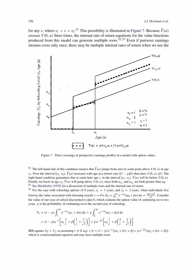
356 J.J. Heckman et al.
for any s, where s1 < s < s2.51 This possibility is illustrated in Figure 7. Because Y(a)
crosses Y(0, a) three times, the internal rate of return equations for the value functionsproduced from this model can generate multiple roots.52,53 Even if pairwise earningsstreams cross only once, there may be multiple internal rates of return when we use the
Figure 7. Three crossings of prospective earnings profiles in a model with option values.
51 The left-hand side of this condition ensures that Y (a) jumps from zero to some point above Y (0, a) at age
s1. Over the interval [s1, s2), Y(a) increases with age at a slower rate ([1 − p]β) than does Y (0, a) (β). Theright-hand condition guarantees that at some later age s, in the interval [s1, s2), Y(a) will be below Y (0, a).Finally, we know at age s2, Y(a) will jump above Y (0, a), since both αs1 and αs2 are both greater than α0.52 See Hirshleifer (1970) for a discussion of multiple roots and the internal rate of return.53 For the case with schooling options of 0 years, s1 = 1 years, and s2 = 2 years, when individuals live
forever, the value associated with choosing exactly s = 0 is Y0 = ∫ ∞0 e−ra(α0 +βa) da = α0r+β
r2 . Considerthe value of one year of school discounted to date 0, which contains the option value of continuing on to twoyears. p is the probability of continuing on to the second year of schooling.
V1 = (1 − p)
∫ ∞1
e−ra(α1 + βa) da + p
∫ ∞2
e−ra(α2 + βa) da
= (1 − p)e−r
[α1
1
r+ β
(1
r+ 1
r2
)]+ p e−2r
[α2
1
r+ β
(2
r+ 1
r2
)].
IRR equates Y0 = V1, so assuming r �= 0, α0r +β = (1−p) e−r [(α1 +β)r +β]+p e−2r [(α2 +β)r +2β],which is a transcendental equation and may have multiple roots.

Ch. 7: Earnings Functions, Rates of Return and Treatment Effects 357
appropriate value function, invalidating their use as a guide to selecting human capitalinvestment projects.
In the more general case of sequential resolution of uncertainty, the schooling transi-tion probability is not exogenous. Multiple roots are even more likely in this case, sincethe transition probability depends on the discount rate. Writing equations out explicitlyin terms of interest rate r , we obtain
Es−1(Vs(r)
) = Prs−1
(εs � Es[Vs+1(r)]
(1 + r)Y s(r)
)Y s(r)Es−1
(εs |εs � Es[Vs+1(r)]
(1 + r)Y s(r)
)+ Prs−1
(εs <
Es[Vs+1(r)](1 + r)Y s(r)
)Es−1[Vs+1(r)]
(1 + r).
In this setting, the natural generalization of the IRR is the value (or values) of rI thatsolves
Ys(rI ) = Es−1(Vs+1(rI ))
1 + rI.
Take a three period example. In this case, the IRR for the second level of schoolingsolves
Y 1(rI ) = Pr1
(ε2 � Y 3(rI )
(1 + rI )Y 2(rI )
)Y 2(rI )
1 + rIE1
(ε2|ε2 � Y 3(rI )
(1 + rI )Y 2(rI )
)+ Pr1
(ε2 <
Y 3(rI )
(1 + r)Y 2(rI )
)Y 3(rI )
(1 + rI )2.
The fact that the continuation probabilities also depend on rI makes multiple roots morelikely. To gain some intuition in this case, take a limiting case where the variance of ε2goes to zero. This implies that the probability of continuing to level three will be either
zero or one, depending on whether or not Y 2 is greater or less than Y 3(1+rI )
. We may,therefore, get two valid solutions to the above IRR equation:
Case 1 (individual always continues): r1I satisfies
Y 1(r1I
) = Y 3(r1I )
(1 + r1I )2
>Y 2(r
1I )
1 + r1I
.
The latter inequality guarantees that the person always wants to continue to schoolinglevel three upon reaching level two.
Case 2 (individual never continues): r2I satisfies
Y 1(r2I
) = Y 2(r2I )
(1 + r2I )
>Y 3(r
2I )
(1 + r2I )2
.
The latter inequality guarantees that the person always stops his schooling at level two.Both of these cases can arise for the same person depending on the realization of
ε2 as long as Var(ε2) > 0, if log earnings are not parallel in experience. Consider thecase where wage gaps are small initially and large later in the life cycle. In this case, r1
I

358 J.J. Heckman et al.
would be less than r2I . In Case 1, the high wage differential later on is not discounted
very much, so the individual always wants to attend schooling level three. A low IRRmust, therefore, equate level one earnings with discounted level three earnings. On theother hand, the high late wage differential may be discounted so much with a highdiscount rate that the individual never chooses to go on to college at that rate. In thiscase, a high IRR, r2
I , must equate level one earnings with discounted level two earnings.These examples are extreme, but multiple roots can arise more generally as long asthe variance of εs is not too large. This type of multiplicity of roots could also comemore directly out of the Comay, Melnik and Pollatschek (1973) type of model, wherethe probability of continuing to level three would be either zero (if individuals do notwant to continue) or p (if individuals wish to continue), depending on the discount rate.Given the lack of parallelism in cross section log earnings profiles, multiplicity of rootsis likely to be empirically important.
These issues call into serious question the usefulness of internal rates of return asa measure of the return to education in an environment where the schooling decisionis dynamic and sequential. A central tool of policy evaluation from classical humancapital theory loses its validity in the presence of option values. Criterion (9) does notsuffer from this criticism and is the appropriate measure of the ex ante rate of returnto use but it is rarely reported. For an exception, see Cunha, Heckman and Navarro(2005) and Cunha and Heckman (2006b) who estimate this rate of return. In the absenceof sequential resolution of uncertainty and option values, Rs,s−1 is the same as theclassical internal rate of return applied to pairwise earnings streams, so it is the naturalgeneralization of that concept.
Empirical work on the option value of schooling is in its infancy. If option valuesare empirically relatively unimportant in models with the sequential resolution of un-certainty, conventional investment evaluation methods based on the IRR may well beinformative on the optimality of schooling investments. Even if option values are negli-gible, the analysis presented throughout this paper suggests that the Mincer model willnot estimate theoretically appropriate rates of return to schooling. In the absence of op-tion values, other key assumptions required to equate Mincer coefficients with internalrates of return are violated. Even in an environment without the sequential resolutionof uncertainty, more general methods of the type presented in Section 4 are required toobtain internal rates of return.
We next turn to an analysis of cross section bias. In doing so, we ignore option values,following conventions in the labor economics literature, and focus on “rates of return” asconventionally measured to concentrate on the issue of whether cross section estimatesof “rates of return” are valid for life cycle “rates of return.”
6. How do cross-sectional IRR estimates compare with cohort-based estimates?
Thus far we have considered estimation of rates of return to schooling using cross-section data which applies the standard synthetic cohort approach followed by most of

Ch. 7: Earnings Functions, Rates of Return and Treatment Effects 359
the literature. For an ex ante analysis it assumes that younger workers base their earn-ings expectations on the current experiences of older workers. For an ex post analysis, itassumes that the experiences of older workers at a point in time will be those of youngerworkers when they reach those ages. If skill prices are changing over time and workersat least partially anticipate these changes, the estimates of the ex ante return to differentschooling levels based on cross-sectional data may not represent the ex ante rates ofreturn governing human capital investment decisions. Similarly, if the environment isnonstationary, the ex post returns of the younger cohort are not accurately estimated.While estimates based on cross-section data reflect current price differentials and op-portunity costs, they do not capture future skill price differentials that forward-lookingindividuals would take into account. The U.S. labor market in recent years is highlynonstationary as are the labor markets of many economies around the world.
If cohorts anticipate future changes in the skill premium, they will base their school-ing decisions on their true cohort-specific rate of return and not the rate of return esti-mated from a cross-section of current workers. However, if individuals do not anticipatethe future price changes, cross-section estimates may better represent their expectationsabout the returns to school. Expectations play a crucial role in determining whethercross-section or cohort-based estimates of the rate of return influence schooling deci-sions.
Another possible source of discrepancy between cross-section and cohort-based rateof return estimates is change in cohort quality, as might arise from changes in the qualityof schools over time. If relative skills for some schooling classes increase permanently,then cohort rates of return jump up with the first ‘new’ cohort and remain higher forall succeeding cohorts. Cross-section estimates only reflect the changes slowly as morehigh quality cohorts enter the sample each year. As a result, they under-estimate truerates of return for cohorts entering the labor market after the change in school quality,with the bias disappearing as time progresses. While future price changes are difficultto predict, changes in cohort or school quality are more identifiable.
Mincer (1974) addressed cross section bias in his pioneering work. He found thatpatterns for wage growth in a 1956 cross-section of male workers were quite similarto the 1956 to 1966 growth in wages for individual cohorts. The empirical discrep-ancy between cross-section and cohort-based estimates was relatively small. Recentanalyses reveal that wage patterns have changed dramatically across cohorts and thatcross-sections no longer approximate cohort or life cycle change [MaCurdy and Mroz(1995), Card and Lemieux (2001)]. While these studies do not agree on whether or notthese changes are due to changes in relative skill prices or cohort quality, there is lit-tle question in the U.S. data that life cycle earnings profiles based on a cross-sectionof workers no longer accurately reflect the true earnings patterns for any given cohort.As a result, the rates of return to schooling estimated from cross-sections of workersreported in the previous section are likely to differ from the rates of return faced bycohorts making their schooling decisions.
Next, we present a cohort analysis focusing on the actual returns earned by eachcohort without taking a position on whether changes in those returns over time are

360 J.J. Heckman et al.
due to changes in cohort quality or skill prices. Arias and McMahon (2001) present asimilar analysis in estimating ex post dynamic rates of return. We study how the actualex post returns earned by individual cohorts compare with returns estimated from across-section of individuals at the time those cohorts made their schooling decisions. Weuse repeated cross-section data from the 1964–2000 Current Population Survey (CPS)March Supplements, comparing cross-section estimates of the return to schooling withestimates that combine all years of the CPS to follow cohorts over their life cycles.Given the sensitivity noted in the previous sections of this chapter to specifications of thefunctional forms of earnings equations, we adopt a flexible earnings specification andcompute internal rates of return to high school completion (12 vs. 10 years of schooling)and college completion (16 vs. 12 years of schooling) that relax the assumptions thatlog earnings are parallel in experience and linear in schooling. Our estimates also takeinto account average marginal tax rates and tuition costs using the time series generatedfrom CPS data.54 Because earnings are not observed at every experience level for anycohort in the sample (an obvious practical problem in estimating cohort rates of return),a fully nonparametric approach is infeasible. To extrapolate the earnings function towork experience levels not observed in the data, we assume that log earnings profilesare quadratic in experience in a specification that allows the intercept and coefficientson experience and experience-squared to vary by schooling class and year or cohort ofdata. We estimate log earnings for each year or for each cohort using regressions of theform
log(Y(s, x)
) = αs + β0sx + β1sx2 + εs,
where the regression coefficients are allowed to vary by schooling group.55 Two sets ofestimates are generated: (i) regressions are estimated separately for each year of CPSdata (to produce a set of cross-section estimates), and (ii) all CPS cross-sections arecombined and separate regressions are estimated for each cohort by following them overtheir life cycles (to produce a set of cohort-based estimates). Both sets of estimates areused to generate predicted life cycle earnings profiles for each cohort or cross-section ofindividuals, which are then used to compute internal rates of return to high school andcollege by the method described in Section 4 setting the residual of the wage equationto its mean.56
54 An average marginal tax rate of 25% is assumed for all years after 1994, the final year of tax rates reportedin Mulligan and Marion (2000). This corresponds to the average of all rates since 1950, after which rateschanged very little from year to year.55 In estimating earnings profiles for those with 10 years of education, we combine individuals with 9–11 years, with separate intercept terms for each of the education levels. This is done to increase precision inestimation. See Appendix B for additional details on the coding of the education variables.56 In addition to the quadratic specification, we also tried using a cubic and quartic in experience to ex-trapolate for the missing experience levels. For cohorts with 25 or fewer years of data, extrapolations basedon higher-order polynomial specifications were unreliable, so we adopted the more parsimonious quadraticspecification.

Ch. 7: Earnings Functions, Rates of Return and Treatment Effects 361
Figure 8a. IRR for 10 vs. 12 years of education for white men (1964–2000 CPS).
Figure 8b. IRR for 12 vs. 16 years of education for white men (1964–2000 CPS).
Figures 8a and 8b show cohort and cross-section high school and college completionIRR estimates for white men, which are based on the CPS estimates reported in Table 8a.Cross-section estimates are shown for each year of the sample from 1964–1995, andcohort-based estimates are shown for cohorts turning age 18 in 1950 through 1983.57
57 We do not estimate returns for cohorts beyond 1983, since there are too few years of earnings observationsfor those cohorts to produce stable and reliable estimates.

362 J.J. Heckman et al.
Table 8aInternal rates of return for white men: best Census and CPS estimates
Schoolingcomparison
Year Mincer Census data CPS data
General spec.(no residualadjustment)
General spec.(residualadjustment)
Cross section Cohort
10 vs. 12 1940 13 24 8 – –1950 11 26 14 – 31960 12 29 16 – 71970 13 29 16 29 341980 11 41 24 38 381990 14 47 31 50 –
12 vs. 16 1940 13 15 13 – –1950 11 7 8 – 141960 12 10 11 – 81970 13 10 10 12 101980 11 8 8 8 141990 14 12 12 14 –
Notes: Mincer estimates make no adjustment for taxes or tuition. Census General Specification estimatesaccount for tuition and progressive taxes with a fully nonparametric wage specification. CPS cross sectionestimates use cross sectional data and a general wage specification accounting for tuition and flat taxes. CPSCohort estimates follow a cohort turning age 18 in the reported year, using a general wage specificationaccounting for tuition and flat taxes. See Appendix B for data description.
The cohort-based estimates reported in Figure 8a reveal relative stability in the re-turn to high school for cohorts making their high school completion decisions priorto 1960, followed by a large increase in the IRR for cohorts making their decisionsover the first half of the 1960s, followed by another period of relative stability. Returnsincreased from around 10% among 1950–60 cohorts to around 40% for post-1965 co-horts. Cross-section based estimates increase slowly but consistently over most of the1964–1995 period. In general, cross-section estimated rates of return under-estimate thetrue rates of return earned by cohorts of white men making their schooling decisions inthe late 1960s and 1970s. However, basic time patterns are consistent across the twosets of estimates. More dramatic differences are observed for the college-going deci-sion of white men as shown in Figure 8b. While cross-section estimates show declining“returns” to college over the 1970s (from 12% down to 8%), cohort-based estimatesshow continually increasing returns from the early 1960s to the early 1980s. The rateof return estimated from cross-sections does not begin to increase until 1980. Cross-section estimates overestimate the rate of return faced by cohorts making their collegeattendance decisions around 1965 by as much as 4 percentage points, while estimates inthe early 1980s under-estimate the return by nearly the same amount. Table 8b reportscomparable numbers for black men.

Ch. 7: Earnings Functions, Rates of Return and Treatment Effects 363
Table 8bInternal rates of return for black men: best Census and CPS estimates
Schoolingcomparison
Year Mincer Census data CPS data
General spec.(no residualadjustment)
General spec.(residualadjustment)
Cross section Cohort
10 vs. 12 1940 9 10 −8 – –1950 10 44 21 – 41960 11 34 16 – 181970 12 39 22 32 491980 12 46 29 55 701990 16 57 42 64 –
12 vs. 16 1940 9 10 6 – –1950 10 5 9 – 151960 11 8 6 – 61970 12 10 10 12 141980 12 11 9 14 171990 16 17 15 16 –
Notes: Mincer estimates make no adjustment for taxes or tuition. Census General Specification estimatesaccount for tuition and progressive taxes with a fully nonparametric wage specification. CPS cross sectionestimates use cross sectional data and a general wage specification accounting for tuition and flat taxes. CPSCohort estimates follow a cohort turning age 18 in the reported year, using a general wage specificationaccounting for tuition and flat taxes. Each CPS estimate is based on three adjoining years/cohorts worth ofdata. See Appendix B for data description.
If the observed discrepancies between cross-section and cohort-based estimated“rates of return” are due to price changes over time that could be at least partly an-ticipated or are due to changing cohort quality, then cross-section estimates would notreflect the ex ante “rates of return” that governed schooling decisions. On the other hand,if changes in skill prices were entirely unanticipated, then cross-section estimates mayprovide a better indication of the ex ante returns governing schooling decisions thanwould the actual ex post returns experienced by each cohort. A better understanding ofthe underlying causes for such dramatic changes in wages and of individual expecta-tions is needed. Buchinsky and Leslie (2000), Carneiro, Hansen and Heckman (2003)and Cunha, Heckman and Navarro (2005) present empirical explorations of alternativeexpectation–formation models. We review methods for estimating agent informationsets in Section 10.
In summary, cross-section estimates of the “rate of return” to schooling should becautiously interpreted, particularly when skill prices are changing over time or whencohort quality is changing. If one is interested in empirically estimating historical ratesof return, a cohort analysis is clearly preferable. Data from the 1964–2000 March CPSsuggest that “returns” estimated from a cross-section of workers are not only biased inlevels, but they also suggest patterns that sometimes differ from those obtained using

364 J.J. Heckman et al.
a cohort-based estimation strategy. If one is interested in estimating the conventionalrates of return governing school investment decisions, then whether to use cross-sectionor cohort-based estimates depends on the extent to which individuals are able to fore-cast future changes in wages and skill prices. We next turn to a review of the recentinstrument-based “rate of return” literature.
7. Accounting for the endogeneity of schooling
Much of the CPS-Census literature on the returns to schooling ignores the choice ofschooling and its consequences for estimating “the rate of return”. It ignores uncertainty.It is static and ignores the dynamics of schooling choices and the sequential revelation ofuncertainty. It also ignores ability bias.58 Economists since C. Reinhold Noyes (1945)in his comment on Friedman and Kuznets (1945) have raised the specter of ability bias,noting that the estimated return to schooling may largely be a return to ability thatwould arise independently of schooling. Griliches (1977) and Willis (1986) summarizeestimates from the conventional literature on ability bias. For the past 30 years, laboreconomists have been in pursuit of good instruments to estimate “the rate of return”to schooling, usually interpreted as a Mincer coefficient. However, the previous sec-tions show that, for many reasons, the Mincer coefficient is not informative on the truerate of return to schooling, and therefore is not the appropriate theoretical construct togauge educational policy. Card (1999) is a useful reference for empirical estimates frominstrumental variable models.
Even abstracting from the issues raised by the sequential updating of information,and the distinction between ex ante and ex post returns to schooling, which we discussfurther below, there is the additional issue that returns, however defined, vary amongpersons. A random coefficients model of the economic return to schooling has been anintegral part of the human capital literature since the papers by Becker and Chiswick(1966), Chiswick (1974), Chiswick and Mincer (1972) and Mincer (1974).59 In its moststripped-down form and ignoring work experience terms, the Mincer model writes logearnings for person i with schooling level Si as
(11)ln yi = αi + ρiSi,
where the “rate of return” ρi varies among persons as does the intercept, αi . For thepurposes of this discussion think of yi as an annualized flow of lifetime earnings. Un-less the only costs of schooling are earnings foregone, and markets are perfect, ρi is apercentage growth rate in earnings with schooling and not a rate of return to schooling.Let αi = α + εαi
and ρi = ρ + ερiwhere α and ρ are the means of αi and ρi . Thus the
58 See Katz and Autor (1999) for a survey. An exception is Angrist and Krueger (1991). For an analysis ofthe quality of their instruments see Staiger and Stock (1997).59 Recall our discussion of the random coefficients model in Section 2.2.

Ch. 7: Earnings Functions, Rates of Return and Treatment Effects 365
means of εαiand ερi
are zero. Earnings equation (11) can be written as
(12)ln yi = α + ρSi + {εαi+ ερi
Si}.Equations (11) and (12) are the basis for a human capital analysis of wage inequality inwhich the variance of log earnings is decomposed into components due to the variancein Si and components due to the variation in the growth rate of earnings with schooling(the variance in ρ), the mean growth rate across regions or time (ρ), and mean schoolinglevels (S). [See, e.g., Mincer (1974), Willis (1986).]
Given that the growth rate ρi is a random variable, it has a distribution that can bestudied using the methods surveyed in Sections 9 and 10. Following the representativeagent tradition in economics, it has become conventional to summarize the distributionof growth rates by the mean, although many other summary measures of the distributionare possible. For the prototypical distribution of ρi , the conventional measure is the“average growth rate” E(ρi) or E(ρi |X), where the latter conditions on X, the observedcharacteristics of individuals. Other means are possible such as the mean growth ratesfor persons who attain a given level of schooling.
The original Mincer model assumed that the growth rate of earnings with schooling,ρi , is uncorrelated with or is independent of Si . This assumption is convenient but is notimplied by economic theory. It is plausible that the growth rate of earnings with school-ing declines with the level of schooling. It is also plausible that there are unmeasuredability or motivational factors that affect the growth rate of earnings with schooling andare also correlated with the level of schooling. Rosen (1977) discusses this problem insome detail within the context of hedonic models of schooling and earnings. A similarproblem arises in analyses of the impact of unionism on relative wages and is discussedin Lewis (1963).
Allowing for correlated random coefficients (so Si is correlated with ερi) raises sub-
stantial problems that are just beginning to be addressed in a systematic fashion in therecent literature. Here, we discuss recent developments starting with Card’s (1999) ran-dom coefficient model of the growth rate of earnings with schooling, a model that isderived from economic theory and is based on the analysis of Becker’s model by Rosen(1977).60 We consider conditions under which it is possible to estimate the mean effectof schooling and the distribution of returns in his model. The next section considers themore general and recent analysis of Carneiro, Heckman and Vytlacil (2005).
In Card’s (1999, 2001) model, the preferences of a person over income (y) andschooling (S) are
U(y, S) = ln y(S) − ϕ(S), ϕ′(S) > 0, and ϕ′′(S) > 0.
The schooling–earnings relationship is y = g(S). This is a hedonic model of schooling,where g(S) reveals how schooling is priced out in the labor market. This specification
60 Random coefficient models with coefficients correlated with the regressors are systematically analyzed inHeckman and Robb (1985, 1986). They originate in labor economics with the work of Lewis (1963). Heckmanand Robb analyze training programs but their analysis clearly applies to estimating the returns to schooling.

366 J.J. Heckman et al.
is written in terms of annualized earnings and abstracts from work experience.61 It as-sumes perfect certainty and abstracts from the sequential resolution of uncertainty thatis central to the modern literature. In this formulation, discounting of future earnings iskept implicit. The first order condition for optimal determination of schooling is
(13)g′(S)
g(S)= ϕ′(S).
The term g′(s)g(s)
is the percentage change of earnings with schooling or the “growth rate”at level s. Card’s model reproduces Rosen’s (1977) model if r is the common inter-est rate at which agents can freely lend or borrow and if the only costs are S yearsof foregone earnings. In Rosen’s setup, an agent with an infinite lifetime maximizes1r
e−rSg(S) so ϕ(S) = rS + ln r , and g′(S)g(S)
= r .Linearizing the model, we obtain
g′(Si)
g(Si)= βi(Si) = ρi − k1Si, k1 � 0,
ϕ′(Si) = δi(Si) = ri + k2Si, k2 � 0.
Substituting these expressions into the first-order condition (13), we obtain that theoptimal level of schooling is Si = (ρi−ri )
k, where k = k1 + k2. Observe that if both
the growth rate and the returns are independent of Si (k1 = 0, k2 = 0), then k = 0 andif ρi = ri , there is no determinate level of schooling at the individual level. This is theoriginal Mincer (1958) model.62
One source of heterogeneity among persons in the model is ρi , the way Si is trans-formed into earnings. [School quality may operate through the ρi for example, as inBehrman and Birdsall (1983), and ρi may also differ due to inherent ability differ-ences.] A second source of heterogeneity is ri , the “opportunity cost” (cost of schooling)or “cost of funds.” Higher ability leads to higher levels of schooling. Higher costs ofschooling results in lower levels of schooling.
We integrate the first-order condition (13) to obtain the following hedonic model ofearnings,
(14)ln yi = αi + ρiSi − 1
2k1S
2i .
To achieve the familiar looking Mincer equation, assume k1 = 0.63 This assumptionrules out diminishing “returns” to schooling in terms of years of schooling. Even under
61 Adding work experience in a multiplicatively separable way produces one Mincer model.62 In that model, aggregate allocations of persons to schooling are determined by an arbitrage condition thatreturns must be equalized across choices.63 The Card model (1999) produces a Mincer-like model where ρi is the Mincer return for individual i. Themean return in the population is E(ρi). It is an ex post return derived under the assumption that log earningsare linear in schooling, contrary to the literature, previously discussed, that shows pronounced nonlinearitiesand sheepskin effects. (See the discussion in Sections 3 and 4.)

Ch. 7: Earnings Functions, Rates of Return and Treatment Effects 367
this assumption, ρi is the percentage growth rate in earnings with schooling, but is notin general an internal rate of return to schooling. It would be a rate of return if therewere no direct costs of schooling and everyone faces a constant borrowing rate. This isa version of the Mincer (1958) model, where k2 = 0, and ri is constant for everyonebut not necessarily the same constant. If ρi > ri , person i takes the maximum amountof schooling. If ρi < ri , person i takes no schooling and if ρi = ri , schooling isindeterminate. In the Card model, ρi is the person-specific growth rate of earnings andoverstates the true rate of return if there are direct and psychic costs of schooling.64
This simple model is useful in showing the sources of endogeneity in the schoolingearnings model. Since schooling depends on ρi and ri , any covariance between ρi − ri(in the schooling equation) and ρi (in the earnings function) produces a random coef-ficient model. Least squares will not estimate the mean growth rate of earnings withschooling unless, COV(ρi, ρi − ri) = 0.
Dropping the i subscripts, the conditional expectation of log earnings given s is
E(ln y|S = s) = E(α|S = s) + E(ρ|S = s)s.
The first term produces the conventional ability bias if there is any dependence be-tween s and raw ability α. Raw ability is the contribution to earnings independent ofthe schooling level attained. The second term arises from sorting on returns to school-ing that occurs when people make schooling decisions on the basis of growth rates ofearnings with schooling. It is an effect that depends on the level of schooling attained.
In his Woytinsky Lecture, Becker (1967), points out the possibility that many ablepeople may not attend school if ability (ρi) is positively correlated with the cost offunds (ri). A meritocratic society would eliminate this positive correlation and mightaim to make it negative. Schooling is positively correlated with the growth rate (ρi) ifCOV(ρi, ρi − ri) > 0. If the costs of schooling are sufficiently positively correlatedwith the growth rate, then schooling is negatively correlated with the growth rate.
Observe that Si does not directly depend on the random intercept αi . Of course, αi
may be statistically dependent on (ρi, ri). In the context of Card’s model, we considerconditions under which one can identify ρ, the mean growth rate of earnings in the pop-ulation as well as the full distribution of ρ. First we consider the case where the marginalcost of funds, ri , is observed and consider other cases in the following subsections.65
7.1. Estimating the mean growth rate of earnings when ri is observed
A huge industry surveyed in Card (1999) seeks to estimate the mean growth rate inearnings, E(ρi), calling it the “causal effect” of schooling. For reasons discussed earlier
64 Recall the discussion of Section 4. From Equation (4) if term 1 is zero, and we assume multiplicativeseparability (or no experience) then ρi (= term 2) = r + term 3 which arises from tuition and psychic costswhere r is the opportunity cost of funds.65 Our discussion is based in part on Heckman and Vytlacil (1998).

368 J.J. Heckman et al.
in this chapter, in general, it is not an internal rate of return. However, it is one of theingredients used in calculating the rate of return as we develop further in Section 8.2.The “causal effect” may also be of interest in its own right if the goal is to estimatepricing equations for labor market characteristics. We discuss some simple approachesfor identifying causal effects before turning to a more systematic analysis in Section 8.
Suppose that the cost of schooling, ri , is measured by the economist. Use the notation“⊥⊥” to denote statistical independence. Assume
ri⊥⊥(ρi, αi).
This assumption rules out any relationship between the cost of funds (ri) and raw abil-ity (αi) with the growth rate of earnings with schooling. For example, it rules outfellowships based on ability. We make this assumption to illustrate some ideas andnot because of its realism. Observing ri implies that we observe ρi up to an additiveconstant. Recall that Si = (ρi−ri )
k, so that ρi = ri + kSi and ρ = E(ρi) = r + kE(Si).
ri is a valid instrument for Si under the assumption that k1 = 0. It is independent ofαi, ρi (and hence εαi , ερi) and is correlated with Si because Si depends on ri . Form
COV(ln yi, ri)
COV(Si, ri)= E{(ri − r)[(αi − α) + (ρi − ρ)(Si − S) + ρSi + ρiS − ρS)]}
E{[
ρi−rik
][ri − r]}=
1kE[(�r)(�ρ)(�ρ − �r)] − ρ
kσ 2
r
−σ 2r
k
,
where �X = X − E(X). As a consequence of the assumed independence between riand (αi, ρi), E[(�r)(�ρ)2] = 0 and E[(�r)2�ρ] = 0, so[
COV(ln yi, ri)
COV(Si, ri)
]= ρ.
Observe that ρ is not identified by this argument if ρi⊥�⊥ri (so the mean growth rateof earnings depends on the cost of schooling).66 In that case, E[(�r)(�ρ)2] �= 0 andE[(�r)2(�ρ)] �= 0. If ri is known and ri = Liγ + Mi , where the Li are observed vari-ables that explain ri and E(Mi |Li) = 0, then γ is identified, provided a rank conditionfor instrumental variables is satisfied.67 We require that Li be at least mean independentof (Mi, ρi, αi). From the schooling equation we can write Si = (ρi −Liγ −Mi)/k andk is identified since we know γ .
Observe that we can estimate the distribution of ρi since ρi = ri + kSi , k is identifiedand (ri , Si) are known. This is true even if there are no instruments L (γ = 0), providedthat ri⊥⊥(ρi, αi). With the instruments that satisfy at least the mean independence con-dition, we can allow ri⊥�⊥ρi and all parameters and distributions are still identified. The
66 The symbol ⊥�⊥ means “not independent of.”67 See, e.g., Greene (2003).

Ch. 7: Earnings Functions, Rates of Return and Treatment Effects 369
model is fully identified provided ri is observed and Li⊥⊥(Mi, ρi, αi).68 Thus, we canidentify the mean return to schooling.
7.2. Estimating the mean growth rate when ri is not observed
If ri is not observed and so cannot be used as an instrument, but we know that ri dependson observed factors Li and Mi , ri = Liγ + Mi and Li ⊥⊥ (Mi, αi, ρi), then theanalysis of Section 7.1 carries over and the mean growth rate ρ is identified. Recall thatln yi = αi + ρSi + (ρi − ρ)Si . Substitute for Si to get an expression of yi in terms of Li ,ln yi = αi + ρi(ρi − Liγ − Mi)/k. We obtain the vector moment equations:
COV(ln yi, Li) = ρ COV(Si, Li),
so ρ is identified from the population moments because the covariances on both sidesare available.69 Partition γ = (γ0, γ1), where γ0 is the intercept and γ1 is the vector ofslope coefficients. From the schooling equation, we obtain
Si = ρi − Liγ1 − Mi
k− γ0
k
= −Li
γ1
k+ ρi − Mi
k− γ0
k.
We can identify γ1/k from the schooling equation, as well as the mean growth rate ρ.However, we cannot identify the distribution of ρi or ri unless further assumptions areinvoked. We also cannot separately identify γ0, γ1 or k. Heckman and Vytlacil (1998)show how to define and identify a version of “treatment on the treated” for growth ratesin the Becker–Card–Rosen model.
7.3. Adding selection bias
Selection bias can arise in two distinct ways in the Becker–Card–Rosen model: throughdependence between αi and ρi and through dependence between αi and ri . Allowingfor selection bias,
E(ln yi |Si) = E(αi |Si) + E(ρiSi |Si) = E(αi |Si) + E(ρi |Si)Si .
If there is an Li that affects ri but not ρi and is independent of (αi,Mi), i.e.,Li⊥⊥(αi, ρi,Mi), and E(ri |Li) is a nontrivial function of Li , in the special case ofa linear schooling model as in Section 7.2,
E(ln yi |Li) = E(αi |Li) + E(ρiSi |Li) = η + ρE(Si |Li).70
68 As we have stressed, the independence conditions are overly strong, but can be weakened to a meanindependence assumption provided that we only seek to recover conditional means.69 One can use the GMM formula presented in Hansen (1982) to construct an efficient estimator if there ismore than one nonconstant element in Li .
70 η = α + ( σ2ρ
k
) − E(ρiMi )k
, where σ 2ρ = VAR(ρi ).

370 J.J. Heckman et al.
Since we can identify E(Si |Li) we can identify ρ. Thus, under the stated conditions,the instrumental variable (IV) method identifies ρ when there is selection bias. In amore general nonparametric case for the schooling equation, which we develop in thenext section of this chapter, this argument breaks down and ρ is not identified when ρi
determines Si in a general way. The sensitivity of the IV method to assumptions aboutspecial features of Card’s model is a simple demonstration of the fragility of the method.We return to this model in Section 10 and use it to motivate recent developments in theliterature on identifying information available to agents when they make their schoolingdecisions.
7.4. Summary
Card’s version of the Becker (1967)–Rosen (1977) model is a useful introduction to themodern literature on heterogeneous “returns to schooling.” ρi is, in general, a person-specific growth rate of log earnings with schooling and not a rate of return. There is adistribution of ρi and no scalar measure is an adequate summary of this distribution.Recent developments in this literature, to which we now turn, demonstrate that standardinstrumental variable methods are blunt tools for recovering economically interpretableparameters.
8. Accounting systematically for heterogeneity in returns to schooling: What doesIV estimate?
To understand what IV estimates in a more general setting, this section analyzes a sim-ple version of (11) in which there are only two levels of schooling. Our discussioncan be generalized [see Heckman and Vytlacil (2005), Heckman, Urzua and Vytlacil(2006)], but for purposes of exposition it is fruitful to focus on a two outcome model.It links IV to the analysis of Willis and Rosen (1979) and Willis (1986), who focus ona two outcome model of schooling in which the ρi of Equation (14) varies in the pop-ulation. Recent research on instrumental variables in the correlated coefficient modelestablishes a close link between IV and the selection model [Heckman (1976)] thatWillis and Rosen apply to obtain their estimates. As shown in Heckman, Urzua andVytlacil (2006), the contrast between IV and selection methods emphasized by Angristand Krueger (1999) and echoed throughout the literature is not valid once the IV methodfor the correlated random coefficient model is correctly understood.
Because schooling is usually received in integer amounts, and most well posed mod-els of schooling choice are based on nonlinear discrete choice frameworks, the simpleCard model abstracts from key features of the schooling choice – earnings outcomemodel which can be captured in a simple way by a discrete outcome model.71 Heckman
71 Card’s model becomes nonlinear if one constrains it to rule out negative schooling and schooling aboveobserved magnitudes.

Ch. 7: Earnings Functions, Rates of Return and Treatment Effects 371
(1997) and Heckman and Vytlacil (1998) show how models of schooling that capturekey features of economic theory are intrinsically nonlinear.
In the model of Section 7, the mean growth rate of earnings with schooling, ρ, was as-sumed to be the parameter of interest without any good justification. While statisticianssometimes call such averages the “average causal effect” (ACE), there is no reason tofocus on this parameter to the exclusion of other parameters that can be derived fromthe distribution of ρi .
Moreover, as we shall show in this section, the instrumental variable estimators setforth in the recent literature do not in general estimate ACE or any of the other standardtreatment effects of schooling on earnings when schooling choices are discrete. They donot estimate rates of return to schooling, nor are they designed to. Instead, they estimatecertain weighted averages of individual growth rates where the weights can sometimesbe negative.
Following Heckman and Vytlacil (2000, 2005, 2007b), Heckman, Urzua and Vytlacil(2006), and Carneiro, Heckman and Vytlacil (2005), consider the following generalizedRoy model of schooling and its “return.” A version of it is applied by Willis and Rosen tothe problem of choice of college using tools developed in the econometrics of selectionbias. Our analysis of this model links the modern IV literature to the classical selectionliterature.72
Let Y1 denote the present value of earnings from college. Y0 is the present value ofearnings from high school. There is a distribution of G = Y1 − Y0 and another distrib-ution of G − C in the population where C denotes the cost of schooling and G denotesearnings gains from college. No single number summarizes either distribution, althoughmuch of the literature focuses on one conditional mean or some other single number asthe object of economic and econometric interest. Attention has focused in recent yearson IV estimates of the coefficient of schooling in a regression of log earnings on school-ing. In the special cases analyzed in Section 7, IV can sometimes identify the meangrowth rate in earnings (E(ρi)) which is usually not the same as the rate of return. Butmore generally, IV does not even identify this parameter. This section considers whatIV estimates in general cases.
If G varies in the population but everyone faces the same C, individuals decide toenroll in school (S = 1) if G − C > 0. Figure 9 plots the hypothetical density of G
in this example, f (G), and also presents the cost that everyone faces, C. Individualswho have values of G to the right of C choose to enroll in school, while those to theleft choose not to enroll. The gross gain for the individuals who choose to go to school,E(G|G � C), is computed with respect to the normalized density of f (G) that is tothe right of C. The marginal return (the return for individuals at the margin) is exactlyequal to C. Figure 9 presents both the average and the marginal return for this example.
Suppose that we want to estimate the effect on earnings of compulsory college at-tendance. Those individuals who are induced to enroll in school by this policy have G
72 Heckman, Urzua and Vytlacil (2006) systematically compare these literatures. See also Heckman andVytlacil (2005, 2007b).

372 J.J. Heckman et al.
Figure 9. Density of absolute returns.
below C (they were not enrolled in school before the policy), and the average “return”for these individuals is E(G|G � C). Alternatively, one might be interested in analyz-ing the effect of a tuition subsidy that changes the cost of attending school from C to C′for everyone in the economy. Those individuals who are induced to enroll in school bythis policy have G below C (they were not enrolled in school before the policy) andG above C′ (they decide to enroll after the policy), and the average “return” for theseindividuals is E(G|C′ < G � C). One needs different parameters to evaluate each ofthese two different policies (E(G|G � C) vs. E(G|C′ < G � C)). Neither is esti-mated by the average growth rate, and hence by the IV method discussed in Section 7.In this example, the marginal entrant into college has a lower return than the averageentrant, and the return for the average student is not the relevant return to evaluate eitherpolicy.73
Standard estimates of the returns to schooling, such as the ones obtained using themethod of least squares, as in the vast literature surveyed by Katz and Autor (1999),or using the method of instrumental variables, as surveyed by Card (1999), are notdesigned to produce either of the policy parameters just described. It is unusual in
73 There is an additional assumption behind this example which we will maintain throughout this chapter:that the policy does not have important general equilibrium effects.

Ch. 7: Earnings Functions, Rates of Return and Treatment Effects 373
the recent literature on the “returns to schooling” for researchers estimating “the ef-fect” of schooling to specify a policy or economic question of interest and address itdirectly. Following Card (1999) and Angrist and Krueger (1999), many define the prob-ability limits of instrumental variable estimators (LATE, defined below) as “the” returnto schooling without stating what economic questions these statistical objects address.Different instruments define different parameters. These parameters answer different,implicitly defined, economic questions. Moreover the commonly accepted interpreta-tion of LATE – that it estimates the returns for those induced to change their schoolingstatus by the change in the instrument – assumes that everyone responds to the instru-ment in the same direction (i.e., all increase their schooling or all decrease it). This is astrong assumption that rules out heterogeneity in the response of schooling choices toinstruments.74
In this section we distinguish between policy parameters of interest, conventionalevaluation parameters and standard estimates of the “returns to schooling.” We showhow these parameters answer different questions, and how we can recover each of themfrom the data. We illustrate the empirical importance of accounting for heterogeneityand the fragility of instruments even in an ideal data set with far richer instrumentsthan are available in the widely used CPS or Census data analyzed in earlier sections ofthis survey. This section draws from Heckman and Vytlacil (2005, 2007b), Heckman,Urzua and Vytlacil (2006) and Carneiro, Heckman and Vytlacil (2005). They estimatethe growth rate of earnings in schooling relevant for evaluating a particular educationpolicy such as a tuition subsidy (in a partial equilibrium framework) and find that it isvery different from the conventional program evaluation parameters usually defined inthe literature, such as the “return to schooling” for the average person, or the “return toschooling” for the average student in college. It also differs from the estimates obtainedby applying least squares or instrumental variables methods, the two methods most oftenused to estimate “returns” to schooling.
We clarify the interpretation of what is usually labeled “ability bias” and “selectionbias” in this literature. Standard intuitions break down in a model of heterogeneousreturns. They can be very misleading when comparing OLS and IV estimates of thegrowth rates of earnings with respect to schooling [see Heckman and Vytlacil (2005)].
Instrumental variables estimates of the “return to schooling” (really growth rates ofearnings with schooling) are usually interpreted as estimating an average “return” toschooling for individuals induced to go to school by changes in the values of the instru-ment, following the LATE (local average treatment effect) interpretation of Imbens andAngrist (1994). Angrist and Krueger (1999) are ardent and influential proponents of thisapproach. We discuss the relationship of LATE to treatment effects and rates of returnbelow.
74 Heckman and Vytlacil (2005) and Heckman, Urzua and Vytlacil (2006) present an extensive discussion ofthis issue.

374 J.J. Heckman et al.
Intuitions about ability bias break down in a particularly serious way if individualshave multiple skills and sort across schooling levels in such a way that the best individ-uals in one schooling level are the worst in the other, and vice versa.75 Heckman andRobb (1985, 1986) make the point that IV does not identify interpretable parameters ina selection model or a generalized Roy model.
8.1. The generalized Roy model of schooling
To focus the discussion, and motivate the empirical literature, we consider a two out-come model. Heckman and Vytlacil (2005, 2007b) and Heckman, Urzua and Vytlacil(2006) extend this discussion to ordered choice and general unordered choice modelswith multiple outcomes.
As noted in Section 7, from its inception, the modern literature on the “returns toschooling” has recognized that returns may vary across schooling levels and across per-sons of the same schooling level.76 The early literature was not clear about the sourcesof variation in returns. The Roy model (1951) and its extensions [see Heckman (1976,1979)], as applied by Willis and Rosen (1979), gives a more precise notion of why re-turns vary and how they depend on S. In the generalized Roy framework, the potentialoutcomes associated with two different schooling levels are generated by two randomvariables (U0, U1):
(15a)ln Y0 = α + U0,
(15b)ln Y1 = α + β + U1,
where E(U0) = 0 and E(U1) = 0 so α (= E(ln Y0)) and α + β (= E(ln Y1)) are themean potential outcomes for ln Y0 and ln Y1 respectively. The common coefficient modelassumes U0 = U1. We implicitly condition on X, the regressors determining potentialoutcomes. Let C(Z) denote costs of schooling measured in proportional terms. The Z
are the variables determining costs. The individual level “causal effect” of educationalchoice S = 1 is
β = ln Y1 − ln Y0 = β + U1 − U0.
In general, this is not a rate of return but a growth rate of earnings with schooling. Thereis a distribution of β in the population.
Observed earnings are written in a “switching regression” form,
ln Y = S ln Y1 + (1 − S) ln Y0 = α + βS + U0
(16)= α + βS + {U0 + S(U1 − U0)
}.
75 As opposed to what we would expect from a single skill model where the best individuals in one sectorwould also be the best individuals in the sector they did not choose if they were placed there instead.76 See Becker and Chiswick (1966), Chiswick (1974) and Mincer (1974).

Ch. 7: Earnings Functions, Rates of Return and Treatment Effects 375
Persons live once and we only observe them in one or the other education state (recallS = 0 or 1). This equation captures the literature on counterfactual states that was devel-oped by Roy (1951). It is also a version of Quandt’s (1958, 1972) switching regressionmodel. It is equivalent to the familiar semilog specification of the earnings–schoolingequation popularized by Mincer (1974), given in Equation (11), which in the currentnotation writes log earnings ln Y as a function of S,
(17)ln Y = α + βS + U,
where U = U0 + S(U1 − U0).77 In terms of the notation of Section 7, U0 = εα ,U1 − U0 = ερ .
In the generalized Roy framework, the choice of schooling is explicitly modeled. Inits simplest form
(18)S ={
1 if ln Y1 − ln Y0 � C ⇐⇒ β � C,
0 otherwise.If agents know or can partially predict β at the time they make their schooling decisions,there is dependence between β and S in Equation (16). This produces the “correlatedrandom coefficient model” that is often applied to general versions of (16). Decisionrules similar to (18) characterize many other economic choices.
The conventional approach to estimating selection models postulates normality of(U0, U1) in Equations (15a) and (15b), writes β and α as linear functions of X andpostulates independence between X and (U0, U1). Parallel normality and independenceassumptions are made for the unobservables and observables in selection equation (18).From estimates of the structural model, it is possible to answer a variety of economicquestions and to construct the various treatment parameters and distributions of treat-ment parameters.78 However in recent years these assumptions have often been viewedas unacceptably strong by empirical labor economists [see, e.g., Angrist and Krueger(1999)].79
A major advance in the recent literature in econometrics is the development of frame-works that relax conventional linearity, normality and separability assumptions to esti-mate various economic parameters. Heckman and Vytlacil (2000, 2005, 2007b) develop
77 For simplicity, throughout this section we suppress explicit notation for dependence of the parameters onthe covariates X unless it is clarifying to make this dependence explicit.78 Willis and Rosen (1979) is an example of the application of the generalized Roy model. Textbook treat-ments of the normal selection model are available in Amemiya (1985) and Ruud (2000). Aakvik, Heckmanand Vytlacil (2005), Heckman, Tobias and Vytlacil (2001, 2003) and Heckman and Vytlacil (2007a) de-rive all of the treatment parameters and distributions of treatment parameters for several parametric modelsincluding the normal. The Heckman, Tobias and Vytlacil papers present one elementary discussion of thenormal selection model applied to the generalized Roy framework. Carneiro, Hansen and Heckman (2003)and Cunha, Heckman and Navarro (2005) estimate the distribution of treatment effects under semiparametricassumptions. We review this work in the last two sections of this chapter.79 A large literature, starting with Heckman and Sedlacek (1985) and exemplified most recently by Blundell,Reed and Stoker (2003) shows that correcting for selection and sectoral choices, a log normality assumptionfor sectoral earnings fits the data well.

376 J.J. Heckman et al.
a framework for estimating rates of return to schooling (mean growth rates of earn-ings with schooling) that do not depend on normality, independence of the conditioningvariables with the regressors, separability or linearity of the estimating equations. Theirwork unites IV and selection models and presents a new local IV approach as a wayto estimate selection models. Heckman, Urzua and Vytlacil (2006) and Heckman andVytlacil (2005) present extensive discussions of the relationship between the two ap-proaches.
Heckman and Vytlacil work with general nonseparable models,
(19)ln Y1 = μ1(X,U1) and ln Y0 = μ0(X,U0).
The growth rate of earnings due to schooling is ln Y1 − ln Y0 = β = μ1(X,U1) −μ0(X,U0), which is a general nonseparable function of (U1, U0). It is not assumed thatX⊥⊥(U0, U1), so X may be correlated with the unobservables in potential outcomes.As demonstrated by Heckman and Vytlacil (2000, 2005, 2007a), one needs exogeneityof X only if one is seeking to make out of sample projections. Like virtually the entiremicroeconomic literature, they ignore any general equilibrium effects of policies onY1, Y0 or β.80
A latent variable model that captures decision rule (18) in a general way is:
(20)S∗ = μS(Z) − US,
S = 1 if S∗ � 0.
In this notation the Z can include all of the variables in the outcome equations plus thevariables in the cost function which are a source of exclusion restrictions. μS(Z) is ageneral function of the observables where US is an unobservable arising from Y1, Y0and C. A person goes to school (S = 1) if S∗ � 0. Otherwise S = 0. In this notation,(Z,X) are observed and (U1, U0, US) are unobserved. US may depend on U1 and U0and the unobservables in C in a general way. The Z vector may include some or all ofthe components of X.
The separability between Z and US in (20) plays a crucial role in the entire mod-ern instrumental variables literature based on LATE and its extensions. It produces the“monotonicity” or “uniformity” condition of Imbens and Angrist (1994). Without theseparability, changes in the instruments in Z can induce two-way flows into and outof treatment and cause IV to break down as a method for estimating treatment effects.See Heckman and Vytlacil (2005, 2007b) and Heckman, Urzua and Vytlacil (2006).Those authors explore the consequences of a simple random coefficient choice modelμS(Z) = Zγ , where γ is a random coefficient that is statistically independent of Z
and US . If γ can assume both positive and negative values, then monotonicity can be
80 Heckman, Lochner and Taber (1998) analyze generalized Roy models of schooling in a general equilibriumframework.

Ch. 7: Earnings Functions, Rates of Return and Treatment Effects 377
violated. But it can also be violated if γ is a nonnegative random vector since differentcomponents of γ would differ across persons experiencing the same change in Z.
The separability that is required to justify (20) and that underlies the entire LATE-based literature cannot be justified in many choice-theoretic models of schooling in-cluding dynamic discrete choice models. The Bellman equation producing the valuefunction in multiperiod settings generates nonseparability between observables and un-observables in the choice equation in early stage decisions even if final stage choices areseparable in those variables [see Cunha, Heckman and Urzua (2006)]. The method ofIV applied to a heterogeneous outcome model is fundamentally asymmetric. It allowsfor heterogeneity in responses to schooling (i.e., it imposes no restrictions on β whichmay be general random variables). At the same time, it restricts the heterogeneity in re-sponses of schooling choices to changes in Z. Consider the special case μs(Z) = Zγ .The “monotonicity conditions” invoked in the recent literature to justify IV as estimat-ing the return to schooling for people induced into schooling by a change in instrumentrules out a random coefficient model for γ except for very special cases. Thus it does notallow for heterogeneity in choices, but it allows for heterogeneity in outcomes. See thediscussion in Heckman and Vytlacil (2005, 2007b) and Heckman, Urzua and Vytlacil(2006).
Heckman and Vytlacil (2001a, 2007b) assume that (a) Z has some variables that shiftμS(Z) given X (the other variables) – an exclusion condition that is standard in the IVliterature; (b) The unobservables (U0, U1, US) are independent of Z given X (a standardinstrumental variables condition) and (c) 0 < Pr(S = 1|X) < 1, so in large samplesthere are some people who have S = 1 and some who have S = 0, so comparisonsbetween treated and untreated persons can be made for those values of X. They makeadditional mild regularity assumptions. Under these conditions it is possible to interpretIV as a weighted average of willingness to pay measures called the marginal treatmenteffect (MTE). A version of this treatment effect was introduced into the econometricsliterature by Björklund and Moffitt (1987) for a linear-in-parameters model.81
Let P(z) be the probability of receiving schooling level 1, S = 1 conditional onZ = z, P(z) ≡ Pr(S = 1|Z = z) = FUS
(μS(z)) where FUSis the distribution of US .
Without loss of generality, one may write US ∼ Unif[0, 1] so μS(z) = P(z).82 (If S∗ =ν(Z) − VS , and VS is a continuous random variable, one can always reparameterize themodel using simple transformation of variable rules so μS(Z) = FVS
(ν(Z)), where FVS
is the distribution of V and US = FV s(VS).) The propensity score P(z) is a monotonictransformation of the mean utility of attending school and we will refer to it as the meanutility.
81 Vytlacil (2002) shows that under the conditions stated in this paragraph, separability (20) implies and isimplied by the monotonicity and independence conditions of Imbens and Angrist (1994) and Angrist andImbens (1995). Heckman and Vytlacil (2005, 2007b) present three alternative definitions of the MTE for ageneral nonlinear model which are equivalent in a linear model.82 We say a random variable is uniformly distributed over [0, 1] if its density is identically equal to 1 overthis interval.

378 J.J. Heckman et al.
When β varies in the population, the growth rate of earnings with schooling is arandom variable and there is a distribution of “causal effects.” There are various waysto summarize this distribution and, in general, no single statistic will capture all aspectsof the distribution.
Many summary measures of the distribution of β are used in the recent literature.Among them are
E(β|X = x) = E(ln Y1 − ln Y0|X = x)
= β(x)
the return to the population average person given characteristics X = x. This quantityis sometimes called “the” causal effect of S.83 Others report the “return” for those whoattend school:
E(β|S = 1, X = x) = E(ln Y1 − ln Y0|S = 1, X = x)
= β(x) + E(U1 − U0|S = 1, X = x).84
This is the parameter emphasized by Willis and Rosen (1979) where E(U1 − U0|S =1, X = x) is the sorting gain – how people who take S = 1 differ from randomlysampled persons.
Another parameter is “the return” for those who are currently not going to school:
E(β|S = 0, X = x) = E(ln Y1 − ln Y0|S = 0, X = x)
= β(x) + E(U1 − U0|S = 0, X = x).
Angrist and Krueger (1991) and Meghir and Palme (2001) estimate this parameter andwe discuss it further below. In addition to these “effects” is the effect for persons in-different between the two levels of schooling, which in the simple Roy model withoutcosts (C = 0) is E(ln Y1 − ln Y0| ln Y1 − ln Y0 = 0) = 0.
Depending on the conditioning sets and the summary statistics desired, a varietyof “causal effects” can be defined. Different causal effects answer different economicquestions. As noted by Heckman and Robb (1986), Heckman (1997) and Heckman andVytlacil (2005, 2007b), under one of two conditions,
I: U1 = U0 (common effect model),
or more generally,
II. Pr(S = 1|X = x, β) = Pr(S = 1|X) (conditional on X,β does not affect choices),
83 It is the Average Treatment Effect (ATE) parameter. Card (1999, 2001) defines it as the “true causal effect”of education. See also Angrist and Krueger (1999, 2001). Our chapter demonstrates that there is no unique“true causal effect.”84 It is the Treatment on the Treated parameter as discussed by Heckman and Robb (1985).

Ch. 7: Earnings Functions, Rates of Return and Treatment Effects 379
all of the mean treatment effects conditional on X collapse to the same parameter. Thesecond condition is the one implicitly used by Mincer (1974). It assumes that schoolingdecisions are not made on the basis of any component of the growth rate β. If nei-ther condition is satisfied, there are many candidates for the title of causal effect. Thisambiguity has produced considerable confusion in the empirical literature as differentanalysts use different definitions in reporting empirical results and many of the estimatesare not strictly comparable.85
Which, if any, of these effects should be designated as “the” causal effect? We havealready noted that conventional “causal effects” are not estimates of a marginal internalrate of return, but instead are estimates of some average growth rate of earnings withschooling. Instead of hoping that a treatment effect or estimator answers an interestingeconomic question, a better approach is to state an economic question and find the an-swer to it. This obvious and traditional approach is not pursued in the recent literature.Heckman and Vytlacil (2001c, 2005, 2007b) develop this approach using a standardwelfare framework. They introduce the notion of a policy relevant treatment effect. Ag-gregate per capita outcomes under one policy are compared with aggregate per capitaoutcomes under another. One of the policies may be no policy at all. For utility crite-rion V (Y ), a standard welfare analysis compares an alternative policy with a baselinepolicy. The Policy Relevant Treatment Effect (PRTE) is
(21)E(V (Y )|Alternative Policy
) − E(V (Y )|Baseline Policy
).
Adopting the common coefficient model, so β = β, a log utility specification (V (Y ) =ln Y) and ignoring general equilibrium effects, where β is a constant, β, the meanchange in welfare is
E(ln Y |Alternative Policy) − E(ln Y |Baseline Policy) = β(�P ),
where (�P ) is the change in the proportion of people induced to attend school by thepolicy. This can be defined conditional on X = x or overall for the population. In termsof gains per capita to recipients, the effect is β. This is also the mean change in logincome if β is a random variable but independent of S if conditions I or II apply. Inthe general case, when agents partially anticipate β, and comparative advantage dic-tates schooling choices, none of the traditional treatment parameters plays the role of β
in (21) or answers the stated economic question. Heckman and Vytlacil (2001c, 2005,2007b) show how the policy relevant treatment effect can be represented as a weightedaverage of the MTE. The weights are given in Table 9b. See Heckman, Urzua and Vyt-lacil (2006) for further examples.
In the empirical literature on the returns to schooling the aim is often to estimateE(β|X = x), although this is unlikely to be the answer to many relevant policy
85 For example, Heckman and Robb (1985) note that in his survey of the union effects on wages, Lewis(1986) confuses these different “effects.” This is especially important in his comparison of cross section andlongitudinal estimates where he inappropriately compares conceptually different parameters.

380 J.J. Heckman et al.
questions. The standard estimation method is instrumental variables. However, in thepresence of heterogeneity and self-selection, we cannot identify E(β|X = x) by us-ing standard instrumental variables methods. Instead, we identify LATE [Imbens andAngrist (1994)], or a weighted average of LATE parameters, which is an instrument de-pendent parameter. It is usually broadly defined as the “average ‘return’ to schoolingfor individuals induced to change their schooling by the observed change in the instru-ment”. The economic interpretation of this parameter is unclear. In general, LATE doesnot correspond to a policy relevant parameter or a rate of return. The LATE parameterof Imbens and Angrist (1994) is often invoked by empirical analysts to justify an in-strumental variable estimate, without providing any precise definition of the economicquestion it addresses.
One way to make this general point is to explore what is estimated by using com-pulsory schooling as an instrument. Compulsory schooling is sometimes viewed as anideal instrument [see Angrist and Krueger (1991)]. But when “returns” are heteroge-neous, and agents act on that heterogeneity in making schooling decisions, compulsoryschooling used as an instrument identifies only one of many possible treatment parame-ters and in general does not estimate a rate of return to schooling.
Compulsory schooling selects at random persons who ordinarily would not beschooled (S = 0) and forces them to be schooled. It is straightforward to establishthat it identifies treatment on the untreated:
E(ln Y1 − ln Y0|X = x, S = 0) = E(β|X = x, S = 0)
but not ATE = E(ln Y1−ln Y0) = β, treatment on the treated TT = E(ln Y1−ln Y0|X =x, S = 1) = E(β|X = x, S = 1), or the marginal internal rate of return.86
Treatment on the untreated answers an interesting policy question. It is informativeabout the earnings gains for a policy directed toward those who ordinarily would notattend school and who are selected into school at random from this pool. If the policythe analyst seeks to evaluate is compulsory schooling then the instrumental variableestimand87 and the policy relevant treatment effect coincide. More generally, if theinstrumental variable we use is exactly the policy we want to evaluate, then the IVestimand and the policy relevant parameter are the same. But whenever that is not thecase, the IV estimand does not identify the effect of the policy when returns vary amongpeople and they make choices of treatment based on those returns.88 For example, if thepolicy we want to consider is a tuition subsidy directed toward the very poorest withinthe pool of nonattenders, then an instrumental variable estimate based on compulsoryschooling will not be the relevant return to evaluate the policy.89
86 See Carneiro, Heckman and Vytlacil (2005).87 An estimand is the probability limit of an estimator.88 See Heckman, Urzua and Vytlacil (2006) for an analysis of this case.89 Heckman and Vytlacil (2005) show that for every policy it is possible in principle to define an instrumentalvariable that generates the correct policy relevant treatment effect. However, such an instrument may not befeasible in any given data set because of support problems. (Support is the range of a random variable whereit has positive density.) Different policies define different policy relevant instrumental variables.

Ch. 7: Earnings Functions, Rates of Return and Treatment Effects 381
8.2. Defining treatment effects in the generalized Roy model and relating them to truerates of return
The index model (18) and (20) can be used to define the marginal treatment effect(MTE),
�MTE(x, uS) ≡ E(β|X = x,US = uS).
This is the mean gain to schooling for individuals with characteristics X = x and withunobservable US = uS .90 It is a willingness to pay measure for an additional year of
Table 9aTreatment effects and estimands as weighted averages of the marginal treatment effect
ATE(x) = ∫ 10 MTE(x, uS) duS (Average Treatment Effect)
TT(x) = ∫ 10 MTE(x, uS)hTT (x, uS) duS (Treatment on the Treated)
TUT(x) = ∫ 10 MTE(x, uS)hTUT (x, uS) duS (Treatment on the Untreated)
PRTE(x) = ∫ 10 MTE(x, uS)hPRT (x, uS) duS (Policy Relevant Treatment Effect)
IV(x) = ∫ 10 MTE(x, uS)hIV (x, uS) duS
OLS(x) = ∫ 10 MTE(x, uS)hOLS(x, uS) duS
Source: Heckman and Vytlacil (2001a, 2001b, 2005, 2007b).
Table 9bWeights∗
hTT (x, uS) = [∫ 1uS
f (p|X = x) dp] 1E(P |X=x)
hTUT (x, uS) = [∫ uS0 f (p|X = x) dp
] · 1E((1−P)|X=x)
hPRT (x, uS) = [FP∗,X(uS)−FP,X(uS)
�P
]hIV (x, uS) = [∫ 1
uS(p − E(P |X = x))f (p|X = x) dp
] 1Var(P |X=x)
hOLS = E(U1|X=x,US=uS)h1(x,uD)−E(U0|X=x,US=uS)h0(x,uS )MTE(x,uS)
h1(x, uS) = [∫ 1uS
f (p|X = x) dp] 1E(P |X=x)
h0(x, uS) = [∫ uS0 f (p|X = x) dp
] 1E((1−P)|X=x)
Source: Heckman and Vytlacil (2001a, 2001b, 2005, 2007b).∗f (p|X = x) is the density of P(Z) given X = x.
90 Björklund and Moffitt (1987) introduced this parameter in the context of the parametric normal Roy model.See Heckman and Vytlacil (2005, 2007a, 2007b) for a discussion of this literature.

382 J.J. Heckman et al.
schooling for persons indifferent between attending or not attending college at a meanutility P(Z) = uS .
Under their assumptions, Heckman and Vytlacil (1999, 2001b, 2005, 2007b) estab-lish that all of the conventional treatment parameters used in the program evaluationliterature are different weighted averages of the MTE where the weights integrate toone. The conventional treatment parameters are the average treatment effect or ATE,E(Y1 −Y0|S = 1, x), and treatment on the untreated or TUT , E(Y1 −Y0|S = 0, x). SeeTable 9a [from Heckman and Vytlacil (2000, 2005, 2007b)] for the treatment parame-ters expressed in terms of MTE and Table 9b for the weights. The analysis of Heckmanand Vytlacil (2001b, 2005, 2007b) unites the selection literature and the modern IV lit-erature using a common analytical framework. Heckman, Urzua and Vytlacil (2006)discuss how to construct the weights.91
These tables also show how one can write the IV and OLS estimates and the PolicyRelevant Treatment Effect as weighted averages of the MTE. The crucial observationto extract from this table is that the weights on MTE are different for IV and for thetreatment parameters. Thus, not only is it true that the treatment parameters are notrates of return, but IV does not in general estimate the treatment parameters.
Figure 10a plots the marginal treatment effect (MTE) derived from a generalizednormal Roy model using the parameterization of (17) and (18) shown at the base ofFigure 10b. It displays the prototypical pattern that the returns to schooling decline forthose persons who have higher costs of schooling (higher US), i.e., for persons lesslikely to attend school.92 The same figure is implicit in the analysis of Willis and Rosenbut they do not develop or exposit it. The treatment effect parameters generated fromthis model are presented in Table 10. It also presents IV and OLS estimates as well asthe sorting gain and selection bias terms for this model.
Figure 10a also displays the weights on MTE used to form ATE (Average Treat-ment Effect), TT (Treatment on the Treated) and TUT (Treatment on the Untreated) fora generalized Roy model (with tuition costs).93 TT overweights the MTE for personswith low values of US who, ceteris paribus, are more likely to attend school. TUT over-weights the MTE for persons with high values of US who are less likely to attend school.ATE weights MTE uniformly. The decline in MTE reveals that the “gross return” (β)
declines with US . Those more likely to attend school (based on lower US) have higher“gross returns” or higher growth rates of earnings with schooling. Not surprisingly, inlight of the shape of MTE and the shapes of the weights, TT > ATE > TUT . Thereis a positive sorting gain (E(U1 − U0|X = x, S = 1) > 0) and a negative selectionbias (E(U0|X = x, S = 1) − E(U0|X = x, S = 0) < 0). Figure 10b displays theMTE and the weights for OLS and for IV using P(Z) as the instrument. IV weights
91 The website for their paper provides software for doing so.92 Recall that S = 1(S∗ > 0) = 1(μS(Z) > US) so that the higher US , the less likely is a person to attendcollege or have S = 1.93 The form of the Roy model we use assumes additive separability and generates U0, U1 and US from acommon unobservable ε. Thus, in this example, the distribution of U1 − U0 given US is degenerate.

Ch. 7: Earnings Functions, Rates of Return and Treatment Effects 383
Figure 10a. Weights for the marginal treatment effect for different parameters.
the MTE more symmetrically and in a different fashion than ATE, TUT or TT . Theshape of the IV weight is prototypical when P(Z) is the instrument. However, for otherinstruments, including individual components of Z, the shapes of the weights are dif-ferent [see Heckman, Urzua and Vytlacil (2006), for further analysis and examples].We present examples of these weights below. OLS weights MTE very differently. Thecontrast between the OLS weight and the IV weight conveys the contrast between theCPS/Census literature and the modern IV literature. In general, neither identifies ATE orthe other treatment effects, and the conventional treatment effects are not rates of return.
To estimate ex post rates of return, it is necessary to account for foregone earningsand direct costs. The treatment effect literature typically accounts for neither and reportsdifferences in labor market payments to different schooling levels. To cast the discussionof Section 4 into the framework of this section, let Y1,t be the earnings of a college-educated person at age t . Let Y0,t be the earnings for a high school-educated personat age t . (To this point in this section we have abstracted from age-dependent growthrates of earnings.) Suppose that it takes τ periods to complete college and that directcosts are Ct per period while in college. The interest rate is r , assumed to be constant.Assume that while in school persons receive no earnings. (If they did, they could helpoffset costs C.) College educated persons retire at age T1. High school educated persons

384 J.J. Heckman et al.
ln Y1 = α + β + U1, σ1 = 0.012,ln Y0 = α + U0, U1 = σ1ε, σ0 = −0.050,S = 1 if Z − US > 0, U0 = σ0ε, σS = −1α = 0.67, US = σSε, ε ∼ N(0, 1),β = 0.2, Z ∼ N(−0.0026, 0.2700).
Figure 10b. Marginal treatment effect vs. linear instrumental variables and ordinary least squares weights.Roy example. Source: Heckman and Vytlacil (2005).
Table 10Treatment parameters in the generalized Roy example
Ordinary least squares 0.1735Treatment on the treated 0.2442Treatment on the untreated 0.1570Average treatment effect 0.2003Sorting gain∗ 0.0440Selection bias† −0.0707Linear instrumental variables‡ 0.2017
∗E[U1 − U0|S = 1] = TT − ATE.†E[U0|S = 1] − E[U0|S = 0] = OLS − TT .‡Using propensity score as the instrument.

Ch. 7: Earnings Functions, Rates of Return and Treatment Effects 385
retire at age T0. One definition of the return to college R is
R =∑T1
t=τY1,t
(1+r)t−τ − ∑T0t=0
(Y0,t+Ct )
(1+r)t∑T0t=0
Y0,t+Ct
(1+r)t
.
This is a version of the Becker (1964) formula. It compares the present values of twoearnings streams realized τ periods apart.
As discussed in Section 3, in the special case assumed by Mincer, log earnings areparallel in experience across schooling categories. For the case of geometric growth anddefining Y 0 = Y0,0 and Y 1 = Y1,τ , earnings may be written as:
Y0,t = Y 0(1 + g)t ,
Y1,t = Y 1(1 + g)t−τ , t � τ,
where g is the growth rate of earnings with age.94 Mincer further assumes thatT1 − T0 = τ so working lives are the same for both schooling classes. The discountedgrowth rate of earnings with experience, e, is
e =T0∑
j=0
(1 + g
1 + r
)j
.
Assume that direct costs (psychic and tuition) are the same per period during the school-ing years and define
A(τ) =τ∑
j=0
(1
1 + r
)j
.
The return in this case is
R = Y 1e − Y 0e − CA(τ)
CA(τ) + Y 0e.
The growth rate of earnings with schooling is
φ = Y 1 − Y 0
Y 0≈ ln Y 1 − ln Y 0.
This is the “Mincer return” to schooling. An alternative expression for the return is
R =φ − CA(τ)
Y 0e
1 + CA(τ)
Y 0e
.
94 Mincer assumes more general period-specific growth rates. The argument in the text can be modified toaccount for this at the cost of more notational complexity.

386 J.J. Heckman et al.
This shows that the Mincer return φ, is greater than the true return, R, whenever costsare positive. When costs are zero (C = 0), R equals the Mincer return, φ. Thus, theMincer assumptions justify the conventional practice of equating growth rates to rates ofreturns, the implicit assumption in the recent literature on estimating rates of return. Ingeneral, if 1+R > (1+r)τ , it pays to go to college; otherwise, it does not. An alternativeway to state this criterion is that it pays to go to college if
1 + φ > (1 + r)τ .
When τ = 1, this simplifies to the conventional criterion that φ > r .The evidence presented in Sections 3 and 4 of this chapter argues strongly against the
practice of equating growth rates with rates of return. Mincer’s parallelism assumptionacross schooling levels (i.e., that growth rates of earnings with experience, g, are thesame for all schooling levels) is not accurate for earnings profiles from more recentdata. Additionally, the evidence presented below in Section 10 points to the existenceof substantial psychic cost components and an adjustment for psychic cost componentssubstantially reduces the rate of return to schooling. The current literature on estimatingrates of return makes none of these adjustments and instead reports the growth rate ofearnings as a “return.” While the growth rate of φ is an ingredient of returns, it is not ingeneral a return, as the expression for R reveals.95
We can use the modern literature to identify growth rates of earnings for personsat different margins of choice. Costs, discount rates and horizons need to be adjustedappropriately to get true rates of return. To our knowledge, this has not been done in thevast IV literature on computing rates of return.
8.3. Understanding why IV estimates exceed OLS estimates of the schooling coefficient
In the generalized Roy model, there are three sources of potential econometric prob-lems; (a) S is correlated with U0; (b) β is correlated with S (i.e., U1 − U0 is correlatedwith S); (c) β is correlated with U0. The relative importance of the problems dependson what question the analyst seeks to answer. Source (a) arises in ability bias or mea-surement error models. Source (b) arises if agents partially anticipate β when makingschooling decisions so that Pr(S = 1|X,β) �= Pr(S = 1|X). In this framework, β is anex post “causal effect,” which may not be known to agents ex ante. In the case where de-cisions about S are made in the absence of information about β, β is independent of S.Source (c) arises from the possibility that the gains to schooling (β) may be dependenton the level of potential earnings in the unschooled state (Y0) as in the Roy model.
When U1 = U0, β is a constant for all persons (conditional on X), and we obtain theconventional IV model as analyzed by Griliches (1977). In this framework, because β isa constant, there is a unique effect of schooling. Indeed, β is “the” effect of schooling,and the marginal effect is the same as the average effect (conditional on X).
95 In addition, in this two choice example, there are no option values. Accounting for them is a factor towardraising the rate of return above the measured growth rate.

Ch. 7: Earnings Functions, Rates of Return and Treatment Effects 387
In the notation of Equation (17), the usual assumption in the literature is thatCOV(S, U0) > 0. Measured schooling S may be correlated with unmeasured U0 be-cause of omitted ability factors. Therefore, when β is constant across individuals, theOLS estimate of the “return” is an upward biased estimate of β:
plim βOLS = β + COV(S, U0)
V (S)> β.
Following Griliches (1977) and the scholars who preceded him, many advocate usinginstrumental variable estimators for β to correct for this problem. If there is an instru-ment Z such that COV(Z, S) �= 0 and COV(Z,U0) = 0, then:
plim βIV = β + COV(Z,U0)
COV(Z, S)= β.
Therefore we expect that βIV < βOLS.However, as noted by Griliches (1977) and Card (1995, 1999, 2001), almost all of
the empirical literature on the returns to schooling shows precisely the opposite pattern:βIV > βOLS. How can one rationalize this finding? One standard explanation is thatschooling is measured with error. This would induce a downward bias in the schoolingcoefficient, which would be corrected by the use of IV.
This simple explanation has been questioned in two different ways. Kane, Rouseand Staiger (1999) claim that measurement error in schooling is nonclassical and there-fore we might not expect the standard attenuation bias that results from nonclassicalmeasurement error.96 Card (1999, 2001) argues that, if measurement error is classical,the amount of measurement error in schooling that would have to exist to justify thelarge gaps between OLS and IV estimates is unreasonably large. He argues that, in fact,schooling is relatively well measured in the U.S., so that the measurement error expla-nation for the empirical regularity is likely to be of second order importance.
The explanation for the empirical regularity that Card (1999, 2001) favors is that thereis heterogeneity in the returns to schooling so β is a random variable and it is correlatedwith schooling. For a model with two levels of schooling, this is just the generalizedRoy model. In this case, it is possible that IV estimates of returns to schooling exceedOLS estimates. Implicitly, his argument has three steps: (1) OLS is an upward biasedestimate of the average “return to schooling” (this is the standard ability bias intuitionin a model in which β is the same for everyone); (2) IV corresponds to an estimate of thereturns to schooling for individuals at the margin;97 and therefore, (3) if the IV estimateof the “return” exceeds the OLS estimate of the “return,” then individuals at the margin
96 Nonclassical measurement error is measurement error of a true variable that is stochastically dependent onthe true value of the variable. Thus the mean, the variance and other moments of the measurement error maydepend on the true value.97 This argument is based on LATE [Imbens and Angrist (1994)]. Card does not provide a precise definitionof the concept. Carneiro, Heckman and Vytlacil (2005) precisely define and estimate the return for the averagemarginal person. See also the discussion in Heckman and Vytlacil (2005).

388 J.J. Heckman et al.
have higher “returns” than the average individual in the economy.98 In our notation, theprobability limits of the least squares and IV estimators are
(22)plim βOLS = β + COV(S, U0)
V (S)+ COV[S, S(U1 − U0)]
V (S),
plim βIV = β + COV[Z, S(U1 − U0)]COV(Z, S)
+ COV(Z,U0)
COV(Z, S)
(23)= β + COV[Z, S(U1 − U0)]COV(Z, S)
.
In general, plim βOLS can be larger than, smaller than or equal to plim βIV . We canrewrite (22) and (23) as:
plim βOLS = β + E(U0|S = 1) − E(U0|S = 0) + E(U1 − U0|S = 1)
= E(β|S = 1) + E(U0|S = 1) − E(U0|S = 0),
plim βIV = β + E(U1 − U0|S = 1)
+ COV[Z, (U1 − U0)|S = 1] Pr(S = 1)
COV(Z, S)
= E(β|S = 1) + COV[Z, (U1 − U0)|S = 1] Pr(S = 1)
COV(Z, S).
Therefore, plim βIV > plim βOLS if COV[Z,(U1−U0)|S=1] Pr(S=1)COV(Z,S)
> E(U0|S = 1) −E(U0|S = 0).99
The assumption implicit in Card’s argument, and in the standard ability bias literature,is that E(U0|S = 1)−E(U0|S = 0) > 0. This condition is satisfied if persons who go tocollege are above average in high school. In such a case, current college graduates wouldbe at the top of the high school wage distribution if they chose to become high schoolgraduates. If this model generates the data, the only way that plim βIV > plim βOLS isif COV[Z,(U1−U0)|S=1] Pr(S=1)
COV(Z,S)> 0.
How plausible is this condition? Recall that Z is a determinant of the cost of school-ing C(Z) and satisfies the standard instrumental variable assumptions. Assume that C
is increasing in Z which is assumed to be scalar.100 As a consequence of these twoconditions,
(24)COV(Z, S) < 0 and COV(Z,U1) = COV(Z,U0) = 0.
98 Card’s model was described in Section 7. It allows for multiple levels of schooling, but assumes a com-mon rate of return across all schooling levels or else reports an average return to schooling across schoolinglevels. Heckman, Urzua and Vytlacil (2006) and Heckman and Vytlacil (2005, 2007b) develop methods foridentifying marginal returns to different schooling levels. For simplicity, we assume a two outcome schoolingmodel.99 This argument appears in Carneiro and Heckman (2002).100 Z may be a vector, but in this example we assume it is a scalar.

Ch. 7: Earnings Functions, Rates of Return and Treatment Effects 389
In the simple two outcome model of schooling, individuals enroll in school if benefitsare higher than costs as is clear from Equation (18) (S = 1 if β − C(Z) = β +(U1 − U0) − C(Z) > 0). In such a model the average individual who attends schoolhas a higher return than the marginal individual (E(β|S = 1) > E(β|β = C(Z))).Furthermore, even though COV(Z,U1 − U0) = 0, COV(Z,U1 − U0|S = 1) > 0 (if anindividual has a high cost, or high Z, he or she will only attend school if he or she alsohas a high U1 − U0). But in that case, because COV(Z, S) < 0, plim βIV < plim βOLS.Implicit in Card’s analysis is the assumption that it is not possible for the average studentto have a higher return than the marginal student and still find that βIV > βOLS. Cardrationalizes βIV > βOLS by assuming that the marginal student with a higher returnthan the average student is out of school because of some external constraint, such as aliquidity constraint so E(β|S = 1) < E(β|β = C(Z)). The less able (lower β) peopleare excluded from school. In Card’s original model, the “returns” to schooling decreasewith the amount of schooling for each individual (k1 < 0 in Section 7), and thoseindividuals whose schooling decision is more sensitive to changes in the instrumenthave relatively little schooling and, as a consequence, relatively high returns.
Drawing on the generalized Roy model, Carneiro and Heckman (2002) and Carneiro,Heckman and Vytlacil (2005) argue instead that the reason why βIV > βOLS is notthat the marginal student has a higher return than the average student (E(β|S = 1) <
E(β|β = C(Z))), but instead that E(U0|S = 1) − E(U0|S = 0) < 0. They show em-pirically, for a nationally representative sample of U.S. white males (NLSY79), that themarginal “return” is below the average for college goers while, simultaneously, βIV >
βOLS. In their setup, COV[Z,(U1−U0)|S=1] Pr(S=1)COV(Z,S)
< 0, E(U0|S = 1) − E(U0|S = 0) < 0
and COV[Z,(U1−U0)|S=1] Pr(S=1)COV(Z,S)
> E(U0|S = 1) − E(U0|S = 0).101 OLS estimatesare downward biased for E(β|S = 1) because E(U0|S = 1) − E(U0|S = 0) < 0.For example, if individuals with S = 1 become teachers and those with S = 0 be-come plumbers, then the latter are better plumbers than the average teacher would be ifhe became a plumber.102 This possibility is featured in Willis and Rosen (1979), whospeculate that, contrary to conventional wisdom, COV(U1, U0) < 0, although, withtheir model, they cannot identify this correlation from the data. Carneiro, Heckman andVytlacil (2005) and Cunha, Heckman and Navarro (2005) identify this covariance andfind evidence that supports the Willis–Rosen conjecture of a negative correlation. Whenanalysts use OLS, they compare E(Y1|S = 1) with E(Y0|S = 0) (see Equation (22)),and since E(Y0|S = 0) > E(Y0|S = 1), the OLS estimate is an underestimate ofE(Y1 − Y0|S = 1).
To summarize, an important lesson from the recent literature is that in a model ofheterogeneous returns, intuitions about ability bias are no longer as simple as in the stan-dard homogeneous returns model with a single measure of ability [Griliches (1977)]. In
101 Carneiro (2002) shows that their conclusions hold for white females and across different data sets.102 In such a model we need to have more than one dimension of ability.

390 J.J. Heckman et al.
such a model, the most able people enroll in school.103 In a more general Roy-typemodel, there can be multiple abilities (in this case, U1 and U0), which can be arbitrarilycorrelated (positively or negatively). The idea that individuals with “high ability” aremore likely to enroll in school is no longer obvious. Recent evidence supports the claimthat the most able persons in the U0 distribution (high school skills) do not go on tocollege. This is true not only in models of schooling, but also in many other models ineconomics where returns to an activity are heterogeneous and people sort into differentactivities based on those returns.104
8.4. Estimating the MTE
We now show how the local IV methods of Heckman and Vytlacil (1999, 2001b, 2005,2007b) can be used to estimate average returns to school for any population of inter-est. Heckman, Urzua and Vytlacil (2006) show how to estimate the MTE and generateall of the weights shown in Table 9b. They also provide software for doing so. UsingEquation (16) the conditional expectation of log Y (= ln Y0(1 − S) + ln Y1S) is
E(ln Y |Z = z) = E(ln Y0|Z = z)
+ E(ln Y1 − ln Y0|Z = z, S = 1) Pr(S = 1|Z = z),
where we keep the conditioning on X implicit. From the index structure generated bydecision rules (18) and (20), we may write this expectation as
E(ln Y |Z = z) = E(ln Y0) + E(β|P(z) � US, P (Z) = P(z)
)P(z).
Observe that the instruments enter the model through the probability of selection or thepropensity score (P (z)). Using P(z) as the instrument, and applying the Wald estimatorfor two different values of Z, z and z′, assuming P(z) < P (z′), we obtain the IVformula:
E(ln Y |P(Z) = P(z)) − E(ln Y |P(Z) = P(z′))P (z) − P(z′)
= β + E(U1 − U0|P(z) � US)P (z) − E(U1 − U0|P(z′) � US)P (z′)P (z) − P(z′)
= E(β|P(z) < US � P(z′)
)= �LATE(
P(z), P (z′)),
103 However, even in the one ability model, Griliches (1977) shows that it is possible that the most able donot enroll in school because their opportunity costs of doing so are too high.104 For example, returns to job training or unionism vary across individuals and individuals make choicesbased on them. The productivity of different inputs varies across firms and they choose different quantitiesof inputs according to the productivity patterns they face (this is relevant for the estimation of productionfunctions). Different consumers have different demand elasticities for a good and their choice of quantitiesdepends on their elasticity.

Ch. 7: Earnings Functions, Rates of Return and Treatment Effects 391
where �LATE is the LATE parameter. This is the average return to schooling for indi-viduals who have US between P(z) and P(z′) (P(z) < US � P(z′)). As we make z
and z′ closer to each other, we identify β for a narrower group of individuals defined interms of their US . The MTE can therefore be estimated by taking a limit of LATE whenz and z′ are arbitrarily close to each other. When U1 ≡ U0 or (U1 − U0)⊥⊥US , cor-responding to the two special cases in the literature, IV based on P(Z) estimates ATE(= β) because the second term on the right-hand side (second line) of this expressionvanishes. Otherwise IV estimates an economically difficult-to-interpret combination ofMTE parameters with weights given in Table 9b.
Another representation of E(ln Y |P(Z) = P(z)) reveals the index structure underly-ing this model more explicitly and writes
E(ln Y |P(Z) = P(z)
)= α + βP (z)
(25)+∫ ∞
−∞
∫ P(z)
0(U1 − U0)f (U1 − U0|US = uS) duS d(U1 − U0).
Differentiating with respect to P(z), we obtain MTE:
∂E(ln Y |P(Z) = P(z))
∂P (z)
= β +∫ ∞
−∞(U1 − U0)f
(U1 − U0|US = P(z)
)d(U1 − U0)
= �MTE(P(z)
).
IV estimates β if �MTE(uS) does not vary with uS . Under this condition E(ln Y |P(Z) =P(z)) is a linear function of P(z). Thus, under our assumptions, a test of the linearity ofthe conditional expectation of ln Y in P(z) is a test of the validity of linear IV for β. Itis also a test for the validity of conditions I and II. Heckman, Urzua and Vytlacil (2006)elaborate on this point.
More generally, a test of the linearity of E(ln Y |P(Z) = P(z)) in P(z) is a testof whether or not the data are consistent with a correlated random coefficient modeland is also a test of comparative advantage in the labor market for educated labor. IfE(ln Y |P(z)) is linear in P(z), standard instrumental variables methods identify “the”effect of S on ln Y . In contrast, if E(ln Y |P(z)) is nonlinear in P(z), then there is het-erogeneity in the return to college attendance, individuals act at least in part on theirown idiosyncratic return, and standard linear instrumental variables methods will not ingeneral identify the average treatment effect or any other of the treatment parametersdefined earlier. This test for nonlinearity in P(Z) as a sign of correlated heterogeneity issimple to execute and interpret. Carneiro, Heckman and Vytlacil (2005) and Heckman,Urzua and Vytlacil (2006) implement it and find evidence in support of nonlinearity inthe data they analyze.
It is straightforward to estimate the levels and derivatives of E(ln Y |P(Z) = P(z))
and standard errors using the methods developed in Heckman et al. (1998). The deriv-

392 J.J. Heckman et al.
ative estimator of MTE is the local instrumental variable (LIV) estimator of Heckmanand Vytlacil (1999, 2001b, 2005, 2007b).105
This framework can be extended to consider multiple treatments, which in this casecan be either multiple years of schooling, or multiple types or qualities of schooling.These can be either continuous [see Florens et al. (2002)] or discrete [see Carneiro,Hansen and Heckman (2003), Heckman and Vytlacil (2005, 2007a, 2007b), Heckman,Urzua and Vytlacil (2006)].
Heckman, Urzua and Vytlacil (2006) establish the close relationship between selec-tion models and instrumental variables models when the response of earnings to changesin education varies among persons. Essentially, IV estimates the derivatives of outcomeequations while the control function estimates them in levels.
8.5. Evidence from the instrumental variables literature
Card (1999) surveys empirical estimates from the instrumental variables literature. Inthe case of the general model presented in this chapter, different instruments identifydifferent weighted averages of the MTE and in general do not identify any interpretableeconomic object such as a rate of return to schooling. The intensity of the search forinstruments Z uncorrelated with (U0, U1) and correlated with S has not been matchedby an equally intense search for an interpretation of what economic question the instru-mental variables estimators answer. As noted by Heckman and Vytlacil (2007a, 2007b)and Heckman, Urzua and Vytlacil (2006), since the question being addressed by therecent literature is not clearly stated, it is not obvious that IV is better than OLS. Theestimates produced from many of the commonly used instruments have large standarderrors in producing any particular parameter of interest except for parameters definedby instruments. On a purely statistical basis there is often little difference between IVand OLS estimates once sampling variation is accounted for. Many of the instrumentsused in this literature are controversial.
Parental education and number of siblings have been used as instruments by Willisand Rosen (1979) and Taber (2001). They tend to produce estimates of “effects” withsmall standard errors. However, they are controversial. It is necessary to assume thatpotential wages in both the college and high school state are independent of familybackground, but many studies show that these are determinants of ability [see Cunha etal. (2006)]. Unless one controls for ability, the quality of the instruments is in question.Many data sets lack direct measures of ability.
Other popular instruments are based on the geographic location of individuals at thecollege going age. If the decision of going to college and the location decision are corre-lated then these instruments are not valid. For example, individuals who are more likelyto enroll in college may choose to locate in areas where colleges are abundant and in-expensive. Distance to college is used as an instrument for schooling by Card (1993),
105 Software is available in Heckman, Urzua and Vytlacil (2006).

Ch. 7: Earnings Functions, Rates of Return and Treatment Effects 393
Kling (2001) and Cameron and Taber (2004). Carneiro and Heckman (2002) show thatdistance to college in the NLSY79 is correlated with a measure of ability and is aninvalid exclusion unless the analyst conditions on ability since ability determines out-comes. Tuition is used as an instrument by Kane and Rouse (1995). Average tuition inthe county of residence may also be a problematic instrument since it is correlated withaverage college quality in the county [see Carneiro and Heckman (2002)]. Finally, lo-cal labor market variables have been used by Cameron and Heckman (1998), Carneiro,Heckman and Vytlacil (2005) and Cameron and Taber (2004). Cameron and Taber usea measure of the local wage. Carneiro, Heckman and Vytlacil use a measure of localunemployment. They also control for long term wages in the county of residence bothin the selection and in the outcome equations, so that the instrument measures businesscycle fluctuations orthogonal to the long term quality of the location of residence.
The CPS and Census data sets lack strong instruments and for that reason few analystsof those data use the method of IV. The “quarter of birth” instrument used by Angrist andKrueger (1991) to identify treatment on the untreated is notoriously weak [see Staigerand Stock (1997)].
Rather than reproduce Card’s (1999) survey, we present some evidence fromCarneiro, Heckman and Vytlacil (2005) on estimates of the MTE using the methodof local instrumental variables and some estimates from Heckman, Urzua and Vytlacil(2006). Both sets of authors use the NLSY data set. The fragility of the estimates andthe large standard errors document the problems that plague the application of the IV todata sets with rich instruments that typically have only a few thousand observations.
The details of the estimation procedure used to generate the numbers reported in thissection are described in Carneiro, Heckman and Vytlacil (2005) and Heckman, Urzuaand Vytlacil (2006). The regressors in the choice equation are a measure of ability (theArmed Forces Qualifying Test or AFQT), number of siblings, mother’s and father’seducation levels, tuition, distance to college, local unemployment rate, and interactionterms. Tuition is a strong predictor of schooling, as are family background and AFQT.The exclusions from the earnings equations are tuition, distance to college, local unem-ployment and opportunity wages in blue collar work at age 17. “Distance to Collegeat 14” and “Local Unemployment Rate at 17” have weak effects. The only strong ex-clusions are tuition and opportunity wages, conditioning on ability.
The density of P(Z) and the support of the estimated propensity score P(Z) (theregion over which P(Z) has positive density) is shown in Figure 11 for the Carneiro,Heckman and Vytlacil (2005) study. It is almost the full unit interval,106 although atthe extremes of the interval the cells of data become very thin. In their estimation ofthe MTE, Carneiro, Heckman and Vytlacil only use values of P between 0.07 and 0.98.
106 Formally, for nonparametric analysis, we need to investigate the support of P(Z) conditional on X.However, the partially linear structure that we will impose below implies that we only need to investigate themarginal support of P(Z).

394 J.J. Heckman et al.
Note: P is the estimated probability of going to college. It is estimated from a logit regression ofcollege attendance on corrected AFQT, father’s education, mother’s education, number of siblings,tuition, distance to college and local unemployment.
Figure 11. Density of P given S = 0 and S = 1 (estimated probability of enrolling in college). Source:Carneiro, Heckman and Vytlacil (2005).
(They trim 5% of the observations in the sample.107) Even after trimming, the sparse-ness of data in the tails results in a large amount of noise (variability) in the estimationof E(Y |X,P (Z) = p) for values of p close to 0.07 or 0.98, which in turn makes prob-lematic estimation of the parameters defined over the full support of US (which requireestimation of E(Y |X,P (Z) = p) over the full unit interval).
The lack of full support of P(Z) means that ATE, TT and TUT are not identifiednonparametrically by the method of instrumental variables. However the MTE can beestimated pointwise for a wide range of evaluation points without full support. Thishighlights what LATE can and cannot do in these data. It can produce a number. It cannotproduce even a conventional treatment effect, much less a rate of return to schooling.The pattern of support of P(Z) is similar in the Heckman, Urzua and Vytlacil (2006)study. See Figure 12 taken from their analysis.
107 The importance of trimming in a semiparametric model similar to the one we use is illustrated inHeckman, Ichimura and Todd (1997).

Ch.7:
Earnings
Functions,R
atesofR
eturnand
TreatmentE
ffects395
Figure 12. Frequency of the propensity score by final schooling decision. HS graduates and four year college graduates – males of the NLSY at age 30. Source:Heckman, Urzua and Vytlacil (2004).

396 J.J. Heckman et al.
Cognitive ability (as measured by AFQT) is an important determinant of the returns toschooling. Simple least squares regressions of log wages on schooling, ability measures,and interactions of schooling and ability (ignoring selection arising from uncontrolledunobservables) have been widely estimated in this and other data sets and generallyshow that cognitive ability is an important determinant of the returns to schooling.108
Carneiro, Heckman and Vytlacil (2005) and Heckman, Urzua and Vytlacil (2006) in-clude AFQT in their model as an observable determinant of the returns to schooling andof the decision to go to college. In the absence of such a measure of cognitive ability,selection arising from unobservables should be important. Most of the data sets that areused to estimate the returns to education (such as the Current Population Survey or theCensus) lack such ability measures.
The test for selection on the individual returns to attending college checks whetherE(ln Y |X,P ) is a linear or a nonlinear function of P . Nonlinearity in P means thatthere is heterogeneity in the returns to college attendance and that individuals selectinto college based at least in part on their own idiosyncratic return (conditional on X).One possible way to implement this test is to approximate K(P ) with a polynomial inP and test whether the coefficients in the terms of the polynomial of order higher thanone are jointly equal to zero. Carneiro, Heckman and Vytlacil test and reject linearity,indicating that a correlated random coefficient model describes the NLSY data.
Carneiro, Heckman and Vytlacil (2005) partition the estimated MTE into two com-ponents, one depending on X and the other on uS ,
MTE(x, uS) = E(ln Y1 − ln Y0|X = x,US = uS)
= μ1(X) − μ0(X) + E(U1 − U0|US = uS).
Figure 13 plots the component of the MTE that depends on US but not on X where theconfidence interval bands are bootstrapped. The estimates are obtained using Robin-son’s (1988) method for estimating partially linear models. E(U1 − U0|US = uS) isdeclining in uS for values of uS below 0.7, and then it is flat and if anything it slightlyrises.109 Returns are annualized to reflect the fact that college goers on average attend3.5 years of college. The most college worthy persons in the sense of having high grossreturns are more likely to go to college (they have low US).110 The magnitude of theheterogeneity in returns is substantial: returns can vary from 13% to 40% per year ofcollege.111
108 See Blackburn and Neumark (1993), Bishop (1991), Grogger and Eide (1995), Heckman and Vytlacil(2001a), Murnane, Willett and Levy (1995), Meghir and Palme (2001).109 Notice that the decision rule is S = 1 if P(Z) − US � 0 so, for a given Z, individuals with a higher US
are less likely to go to college.110 US may be interpreted as the unobservable cost of college.111 The bootstrapped confidence intervals are very wide. However, the estimates of each point of the curveare highly correlated which will reduce the imprecision of the implied treatment parameters. For example,Carneiro, Heckman and Vytlacil can reject (at the 10% level) the hypothesis that MTE(x, US = 0.05) =MTE(x, US = 0.5) (although, they cannot reject that MTE(x, US = 0.5) = MTE(x, US = 0.95)).

Ch. 7: Earnings Functions, Rates of Return and Treatment Effects 397
Note: To estimate the function in this figure (E(Y1 − Y0|X,US)) we use a two step procedure. Wefirst estimate μ0(X) and μ1(X) from a regression of log wages on polynomials in X, interactions ofpolynomials in X and P , and a nonparametric function of P (where P is the predicted probabilityof attending college). We estimate a partially linear model. X includes experience, corrected AFQTand local unemployment. Then we compute the residual of this regression by subtracting μ0(X) +P ∗ [μ1(X) − μ0(X)] from log wages. Finally we estimate the nonlinear function in the figure byrunning a local quadratic regression of this residual on P and taking the coefficients on the linearterm. Then we add a constant term to this function which is simply the average of μ1(X) − μ0(X).E(Y1 −Y0|X,US) is divided by 3.5 to account for the fact that individuals that attend college have onaverage 3.5 more years of schooling than those who do not. Therefore these correspond to estimatesof returns to one year of college. The confidence interval bands are bootstrapped (250 replications).
Figure 13. E(Y1 − Y0|X,US) estimated using locally quadratic regression (averaged over X). Source:Carneiro, Heckman and Vytlacil (2005).
The wide standard error bands are symptomatic of a phenomenon that plagues theentire IV literature. Estimates are not precisely determined. Figure 14 from Heckman,Urzua and Vytlacil (2004) reveals a similar pattern and a wide band of standard errors.Over broad intervals the confidence bands include zero indicating no effect of schoolingon earnings. If β is independent of S, the MTE is flat. The evidence clearly rejects thisso a correlated random coefficient model describes their data but there is a considerableloss in precision in using instrumental variables.

398 J.J. Heckman et al.
Figure 14. MTE with confidence interval. Sample of HS graduates and four year college graduates – malesat age 30 – nonparametric. Source: Heckman, Urzua and Vytlacil (2004).
Table 11 presents estimates of different summary measures of returns to one yearof college for two models from Carneiro, Heckman and Vytlacil (2005). In the firstcolumn they use family background as an exclusion and in the second they do not. Thepoint estimates are similar in both models but they are more precise in the first one,and therefore we focus on those. However, this precision in estimation is obtained byusing what many would argue are invalid exclusion restrictions. These parameters areobtained by using the appropriate weights for each parameter [see Carneiro, Heckmanand Vytlacil (2005)].
The limited support of P near the boundary values of P = 0 and P = 1 creates apractical problem for the computation of the treatment parameters such as ATE, TT , andTUT , since MTE cannot be estimated for values of US outside the support of P . Thesparseness of the data in the extremes does not allow accurate estimation of the MTE atevaluation points close to 0 or 1. The numbers presented in Table 11 are constructed afterrestricting the weights to integrate over the region [0.07, 0.98]. These can be interpretedas the parameters defined in the empirical (trimmed) support of P(Z), which is close tothe full unit interval.112
The sensitivity of estimates to lack of support in the tails (P = 0 or P = 1) isimportant for parameters, such as ATE or TT , that put substantial weight on the tails ofthe MTE distribution. Even with support over most of the interval [0, 1], such parameters
112 Alternative ways to deal with the problem of limited support are to construct bounds for the parametersor to use a parametric extrapolation outside of the observed support. Bounds on the treatment effects aregenerally wide even though the support is almost full. Parametric extrapolation outside of the support ispotentially sensitive to the choice of extrapolation model. Estimates based on locally adapted extrapolationsshow much less sensitivity than do estimates based on global approximation schemes. See Carneiro, Heckmanand Vytlacil (2005) for further discussion.

Ch. 7: Earnings Functions, Rates of Return and Treatment Effects 399
Table 11Estimates of various returns to one year of college
Family background is exclusion Family background is not exclusion0.07 < P < 0.98 0.07 < P < 0.98
Average treatment effect 0.2124 0.1638(0.0648) (0.0916)[0.0069; 0.2641] [−0.0074; 0.2955]
Treatment on the treated 0.3202 0.2279(0.1103) (0.1171)[0.0045; 0.4094] [−0.0036; 0.3820]
Treatment on the untreated 0.1042 0.0897(0.0802) (0.1285)[−0.0027; 0.2522] [−0.1400; 0.3024]
Policy relevant treatment effect 0.2489 0.1905($500 tuition subsidy) (0.0854) (0.1651)
[0.0024; 0.3520] [−0.1037; 0.3602]Ordinary least squares 0.0788 0.0796
(0.0091) (0.0114)[0.0654; 0.0955] [0.0614; 0.0983]
Instrumental variables 0.1649 0.1530(0.0389) (0.0758)[0.0888; 0.2166] [0.0036; 0.2479]
Notes: Bootstrapped 5–95% standard errors (in parentheses) and confidence intervals (in brackets) are pre-sented below the corresponding coefficients (250 replications).Source: Carneiro, Heckman and Vytlacil (2005).
cannot be identified unless 0 (for both ATE and TT) and 1 (for ATE) are contained in thesupport of the distribution of P(Z). Estimates of these parameters are highly sensitive toimprecise estimation or extrapolation error for E(Y |X,P (Z) = p) for values of p closeto 0 or 1. Even though empirical economists often seek to identify ATE and TT , usuallythey are not easily estimated nor are they always economically interesting parameters.As we have stressed repeatedly, they are not rates of return.
Integrating only over P(Z) in the interval [0.07, 0.98], Table 11 reports estimates ofthe average annual return to college for a randomly selected person in the population(ATE) of 21.24%, which is between the annual return for the average individual whoattends college (TT), 32.02%, and the average return for high school graduates whonever attend college (TUT), 10.42%. Card reports IV estimates between 6 and 16%using different instruments but, as previously noted, different instruments weight MTEdifferently and answer different implicit questions. None of these numbers correspondsto the average annual return to college for those individuals of poor backgrounds whoare induced to enroll in college by a $500 tuition subsidy (PRTE), which is 24.89%.113
113 The policy consists of a subsidy of $500 for individuals who have higher than median ability and forwhom both parents have less than a high school degree. The purpose of this simulation is to approximate a

400 J.J. Heckman et al.
This is the relevant return for evaluating this specific policy using a Benthamite welfarecriterion. It is below TT , which means that the marginal entrant induced to go to collegeby this specific policy has an annual return well below (ten log points) that of the averagecollege attendee.
Carneiro, Heckman and Vytlacil (2005) compare all of these estimated summarymeasures of returns with the OLS and IV estimates of the annual return to college, wherethe instrument is P (Z), the estimated probability of attending college for individualswith characteristics Z. OLS estimates ATE if S and X are orthogonal to U0+S(U1−U0).Since the returns estimated by OLS and by IV both depend on X, they evaluate the OLSand IV returns at the average value of X for individuals induced to enroll in collegeby a $500 tuition subsidy,114 so that they can compare these estimates with the policyrelevant treatment effect. The OLS estimate of the return to a year of college is 7.88%while the IV estimate is 16.49%.115 Only by accident does IV identify policy relevanttreatment effects when the MTE is not constant in US and the instrument is not thepolicy. Carneiro, Heckman and Vytlacil (2005) display the weights for all the treatmentparameters reported in this section.
Carneiro, Heckman and Vytlacil (2005) report that βOLS < βIV . This finding is com-mon in the literature [Card (2001)]. At the same time, the returns to schooling are higherfor individuals more likely to enroll in college, which means that the average return forthe marginal individual is below the return for the average student in college. As ex-plained in Section 8.3 and confirmed in the empirical work of Carneiro, Heckman andVytlacil (2005) reported here and in Cunha, Heckman and Navarro (2005), this is possi-ble because the conventional measure of selection bias (E(U0|S = 1) − E(U0|S = 0))
is negative and not positive, as is implicitly assumed in Card (1999, 2001) and in most ofthe empirical literature. In a model of heterogeneous returns, standard intuitions aboutinstrumental variables and ability bias break down. Carneiro, Heckman and Vytlacil(2005) confirm the conjecture of Willis and Rosen (1979). The evidence of Cunha,Heckman and Navarro (2005) shows that the single skill or efficiency units representa-tion of the labor market which is implicit in most of the literature is invalid.
Table 12, taken from the analysis of Heckman, Urzua and Vytlacil (2004), demon-strates the sensitivity of IV estimates to the choice of instruments and to whether or
means tested tuition subsidy for high ability individuals. The standard error of this estimate is quite high, eventhough it overweights the MTE where it is more precisely estimated. The reason is that the flexible form weuse for the selection equation, although useful for the estimation of the MTE, creates some imprecision inthe policy simulation because not all the coefficients on the terms involving tuition are precisely estimated,at least for this policy. It is easier to simulate policies in models where tuition enters the choice equation ina simpler way, although in some cases the standard errors of the MTE become larger because it is important(for the standard errors) to be flexible in the way the instruments affect choices. See Carneiro, Heckman andVytlacil (2005) for further details.114 This is obtained by integrating X with respect to fX(x|PRT) = fX(x|μS(Z) − US < 0, μS(Z′) − US
� 0).115 When they compute the IV parameter by weighting up the MTE using the IV weights, they get an estimateof 12.12%, which is close to the IV estimate we obtain using the direct method.

Ch. 7: Earnings Functions, Rates of Return and Treatment Effects 401
not the estimates are conducted on samples where there is full support. As Figure 12reveals, there are many intervals over which support is less than full, or very thin. InTable 12, for the full sample (first column) or the common support sample (second col-umn), the IV estimates are all over the map. [Their estimates should be divided by 3.5to get the annual returns to college reported in Carneiro, Heckman and Vytlacil (2005).]The final three columns show the IV based on an estimated MTE using (a) a parametricnormal model (third column); (b) a semiparametric polynomial estimation method and(c) a nonparametric method based on local linear regression. The weights used to pro-duce the IV estimates are given in Table 9b and are tailored to each estimation situation.There is close agreement between the two semiparametric methods and they are verydifferent from the estimates in the third column that assume normality. The instability
Table 12Instrumental variables estimates NLSY–HS graduates and four-year college graduates males at age 30∗
Instruments Standard IV IV-MTE (common support)§
Full sample† Common
support‡Parametric Polynomial Nonparametric
Number ofsiblings at 14
0.983 1.122 0.390 0.634 0.634(0.512) (0.591) (0.121) (0.163) (0.160)
Family income in1979 (thousands)
1.667 1.803 0.416 0.590 0.612(0.432) (0.630) (0.121) (0.143) (0.147)
Local wage ofHS graduates atcounty level atage 17
94.600 41.400 0.407 0.591 0.618(1713.300) (334.000) (0.141) (0.269) (0.190)
Two year coll.grad’s local wageat age 17
5.008 5.394 0.426 0.600 0.622(4.077) (4.941) (0.135) (0.216) (0.188)
Four year coll.grad’s local wageat age 17
2.742 3.149 0.428 0.614 0.629(1.093) (1.537) (0.125) (0.187) (0.162)
Local unemp.rate of HSgraduates atcounty level atage 17
0.675 0.612 0.203 0.523 0.526(0.604) (0.675) (0.442) (33.651) (15.377)
Two year coll.grad’s localunemploymentrate at age 17
0.210 0.187 0.363 0.580 0.588(0.579) (0.727) (0.260) (1.824) (1.927)
Four year coll.grad’s localunemploymentrate at age 17
3.465 4.480 0.405 0.554 0.588(13.476) (11.586) (0.144) (0.294) (0.220)
(Continued on next page)

402 J.J. Heckman et al.
Table 12(Continued)
Instruments Standard IV IV-MTE (common support)§
Full sample† Common
support‡Parametric Polynomial Nonparametric
Distance to a twoyear college
3.369 4.603 0.416 0.606 0.621(3.223) (6.282) (0.139) (0.186) (0.165)
Distance to a fouryear college
4.810 7.440 0.415 0.629 0.634(5.180) (12.150) (0.120) (0.170) (0.161)
Two year collegetuition
−2.637 −1.870 0.417 0.798 0.677(3.321) (2.172) (0.767) (8.690) (5.931)
Four year collegetuition
12.500 72.300 0.436 0.650 0.642(42.780) (1465.920) (1.248) (0.729) (0.604)
Propensity score 0.496 0.505 0.420 0.572 0.604(0.093) (0.103) (0.121) (0.138) (0.143)
∗We excluded the oversample of poor whites and the military sample.†The IV estimates and the standard deviations (in parentheses) are computed applying the traditional formulaeto the full sample. The number of observations in our sample is 982.‡The IV estimates and the standard deviations (in parentheses) are computed applying the traditional formulaeto the common support sample. This sample contains only observations for which the estimated propensityscore belongs to the common support of the propensity score between the control (HS graduates) and treat-ment group (4 year college graduates) (912 observations).§In the first column the IV estimates are computed by taking the weighted sum of the MTE estimated usingthe parametric approach. In the second column the IV estimates are computed by taking the weighted sumof the MTE estimated using a polynomial of degree 4 to approximate E(Y |P). The IV estimates in the lastcolumn are computed by taking the weighted sum of the MTE estimated using the nonparametric approach.The propensity score (Prob(D = 1|Z = z)) is computed using the instruments presented in the table as wellas two dummy variables as controls for the place of residence at age 14 (south and urban), and a set of dummyvariables controlling for the year of birth (1958–1963). The standard deviations (in parentheses) are obtainedusing bootstrapping (100 draws).Source: Heckman, Urzua and Vytlacil (2004).
manifest in the numbers reported in the first two columns is reduced by using the MTE.But the instability is manifest in a number of studies in the literature.
Table 13 shows estimates of the various treatment parameters based on the threeversions of the MTE. There is a sharp contrast in the estimates produced from theparametric and nonparametric approaches. The different treatment parameters estimatedifferent objects. The LATE estimators, defined for different points of evaluation P(Z)
(given by the arguments in parentheses) estimate very different numbers.Figures 15a and 15b from Heckman, Urzua and Vytlacil (2004) graph the weights
for the MTE for some of the instruments used to generate the numbers in Table 12.The weights for P(Z) as an instrument are very different from the weights for four-year college tuition (Figure 15a) and especially two-year college tuition (Figure 15b).

Ch. 7: Earnings Functions, Rates of Return and Treatment Effects 403
Table 13Treatment parameter estimates NLSY–HS graduates and four-year college graduates males at age 30∗
Treatment parameter† Parametric‡ Polynomial‡ Nonparametric§
Treatment on the treated 0.362 0.758 0.696(0.123) (0.201) (0.181)
Treatment on the untreated 0.509 0.687 0.652(0.149) (0.142) (0.167)
Average treatment effect 0.455 0.713 0.668(0.127) (0.153) (0.151)
LATE(0.62, 0.38) 0.483 0.59 0.659(0.138) (0.185) (0.192)
LATE(0.79, 0.55) 0.555 1.04 0.792(0.175) (0.269) (0.245)
LATE(0.45, 0.21) 0.412 0.157 0.383(0.120) (0.184) (0.159)
∗We excluded the oversample of poor whites and the military sample.†The treatment parameters are estimated by taking the weighted sum of the MTE estimated using a polynomialof degree 4 to approximate E(Y |P).‡The treatment parameters were estimated by taking the weighted sum of the MTE estimated using the para-metric approach.§The treatment parameters were estimated by taking the weighted sum of the MTE estimated using the non-parametric approach. The standard deviations (in parentheses) are computed using bootstrapping (100 draws).Source: Heckman, Urzua and Vytlacil (2004).
This accounts for why different instruments define different parameters in terms of theirweighting of a common MTE function. It is the MTE function and not an IV estimate thatplays the role of a policy invariant parameter in the modern literature on instrumentalvariables.
8.6. The validity of the conventional instruments
This section examines the validity of conventional instruments in the NLSY data whichis unusually rich. Many data sets on earnings and schooling do not possess measuresof cognitive ability. For example, the CPS and many other data sets used to estimatethe returns to schooling surveyed in Katz and Autor (1999) do not report measures ofcognitive ability. In this case, ability becomes part of U1, U0 and US instead of beingin X.
The assumption of independence between the instrument and U1 and U0 implies thatthe instruments have to be independent of cognitive ability. However, the instrumentsthat are commonly used in the literature are correlated with AFQT, a widely used mea-sure of ability. The first column of Table 14a shows the coefficient of a regression ofeach instrument (Z) on college attendance (S), denoted by βS,Z . With the exceptionof the local unemployment rate, all candidate instruments are strongly correlated with
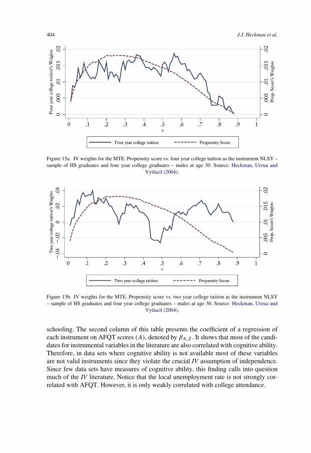
404 J.J. Heckman et al.
Figure 15a. IV weights for the MTE. Propensity score vs. four year college tuition as the instrument NLSY –sample of HS graduates and four year college graduates – males at age 30. Source: Heckman, Urzua and
Vytlacil (2004).
Figure 15b. IV weights for the MTE. Propensity score vs. two year college tuition as the instrument NLSY– sample of HS graduates and four year college graduates – males at age 30. Source: Heckman, Urzua and
Vytlacil (2004).
schooling. The second column of this table presents the coefficient of a regression ofeach instrument on AFQT scores (A), denoted by βA,Z . It shows that most of the candi-dates for instrumental variables in the literature are also correlated with cognitive ability.Therefore, in data sets where cognitive ability is not available most of these variablesare not valid instruments since they violate the crucial IV assumption of independence.Since few data sets have measures of cognitive ability, this finding calls into questionmuch of the IV literature. Notice that the local unemployment rate is not strongly cor-related with AFQT. However, it is only weakly correlated with college attendance.

Ch. 7: Earnings Functions, Rates of Return and Treatment Effects 405
Table 14aRegression of instrumental variables (Z) on schooling (S) and AFQT (A)
Instrumental variable βS,Z βA,Z F-Stat
Number of siblings −0.0302 −0.0468 15.04(0.0078) (0.0141)
Mother’s education 0.0760 0.1286 157.56(0.0060) (0.0110)
Father’s education 0.0582 0.0986 201.33(0.0041) (0.0075)
Average county tuition at 17 −0.0062 −0.0044 13.32(0.0017) (0.0031)
Distance to college at 14 −0.0038 −0.0081 8.56(0.0013) (0.0023)
State unemployment rate at 17 −0.0052 −0.0038 0.42(0.0081) (0.0148)
Source: Carneiro, Heckman and Vytlacil (2005).
The third column of Table 14a presents the F-statistic for the test of the hypothe-sis that the coefficient on the instrument is zero in a regression of schooling on theinstrument. Staiger and Stock (1997) suggest using an F-statistic of 10 as a thresholdfor separating weak and strong instruments.116 The table shows that the local unem-ployment variable has an F statistic well below 10 which suggests that it is a weakinstrument when used by itself. Therefore either the candidate instrumental variable iscorrelated with ability or it is weakly correlated with schooling.
Table 14b presents coefficients of regressions of each instrument on schooling andability, after controlling for family background variables (number of siblings andparental education). Conditioning on family background weakens the correlation be-tween AFQT and the instruments. However the F-test for a regression of schooling onthe residualized instrument is low by Staiger–Stock standards. Residualizing on familybackground attenuates the correlation between the instruments and ability but also be-tween the instruments and schooling. The strength of this dependence is reported in thethird column of Table 14b.
The instrument used by Carneiro, Heckman and Vytlacil (2005) is P(Z). Regressingschooling on polynomials in experience, corrected AFQT, number of siblings, mother’seducation, father’s education (the variables we include in the wage regression) andP(Z), the F-statistic of the coefficient on P is 33.76. By including AFQT in the wageregression they attenuate the possibility of using invalid instruments. By using an in-dex of instruments instead of a single instrument, it is possible to overcome the weak
116 In a recent paper Stock and Yogo (2002) propose a different test. However they still find that the rule ofthumb first proposed in Staiger and Stock (1997) works well in general.

406 J.J. Heckman et al.
Table 14bResidualized regression of instrumental variables (Z) on schooling (S) and
AFQT (A)
Instrumental variable βS,Z βA,Z F-Stat
Average county tuition at 17 −0.0041 −0.0009 6.81(0.0015) (0.0029)
Distance to college at 14 −0.0008 −0.0032 0.53(0.0012) (0.0022)
State unemployment rate at 17 −0.0027 0.0005 0.13(0.0075) (0.0138)
Source: Carneiro, Heckman and Vytlacil (2005).
instrument problem. Furthermore, using an index of instruments instead of a single in-strument tends to reduce support problems for any instrument. Even if one instrumenthas limited support, other instruments can augment the support of P . Observe that theIV estimates based on P(Z) are more stable in Table 12 than are the estimates based onthe individual components.
8.7. Summary of the modern literature on instrumental variables
Heckman and Vytlacil (2001a, 2005, 2007b) show how to write different conventionalmean parameters and IV estimates as weighted averages of the marginal treatment effect(MTE). In a model with heterogeneous responses, different instruments define differentparameters. Unless the instruments are the policies being studied, these parameters an-swer well-posed economic questions only by accident. It is possible to identify andestimate the MTE using a robust nonparametric selection model. Their method allowsthem to combine diverse instruments into a scalar instrument motivated by economictheory. This combined instrument expands the support of any one instrument, and allowsthe analyst to perform out-of-sample policy forecasts. Focusing on a policy relevantquestion, they construct estimators based on the MTE to answer it, rather than hopingthat a particular instrumental variable estimator happens to answer a question of eco-nomic interest. The approach based on the MTE unites the selection and IV literatures.As noted by Heckman, Urzua and Vytlacil (2006), both methods use P(Z) but oneconditions on it (the selection model) while the other (the IV literature) does not.
The recent literature confirms in a semiparametric setting a central claim of theparametric Willis and Rosen (1979) analysis [Carneiro, Hansen and Heckman (2003),Cunha, Heckman and Navarro (2005)]. Individuals sort into schooling on the basis ofboth observed and unobserved gains where the observer is the economist analyzing thedata. Moreover, as noted by Willis and Rosen (1979), it is not possible to rationalize la-bor market data with the single skill (or efficiency units) model that governs most of thestandard intuitions about ability bias in schooling. In fact, these intuitions break down in

Ch. 7: Earnings Functions, Rates of Return and Treatment Effects 407
a general model of heterogeneous returns, and lead to potentially wrong interpretationsof the data.
Instrumental variables are not guaranteed to estimate policy relevant treatment pa-rameters or conventional treatment parameters. Different instruments define differentparameters, and in the empirical analysis of Carneiro, Heckman and Vytlacil (2005)and Heckman, Urzua and Vytlacil (2006) they produce wildly different “effects” ofschooling on earnings. The current practice of reporting IV estimates as “returns” toschooling defines the parameter being identified by an econometric method and not byan economic question. Our examples show that the IV method does not produce an eco-nomically interesting or interpretable parameter, and in general does not estimate a rateof return. Different IV estimators weight the MTE differently and are not comparable intheir economic content.
Even granting the validity and the strength of the instruments, the entire recentIV enterprise for correlated random coefficient models is premised on a fundamentalasymmetry. Returns (growth rates) are allowed to be heterogeneous in a general way.Schooling may either increase or decrease rates of return. However, choices are not per-mitted to be heterogeneous in a general way [Heckman and Vytlacil (2005), Heckman,Urzua and Vytlacil (2006)]. The monotonicity assumptions (or index structure assump-tions embodied in (18) or (20) so that schooling is determined by an index of “netutility” where the observables are separable from the nonobservables) impose the con-dition that all persons respond in the same way in their schooling choices for any changein Z. Thus if increasing a coordinate of Z, say Z1, increases schooling for one person,the same increase cannot decrease schooling for anyone else. This condition rules outheterogeneity in the choice equations. These conditions are at odds with a variety of eco-nomic models for schooling such as models for dynamic discrete choice [see Heckmanand Navarro (2006)]. See Belzil and Hansen (2005) for an interesting contrast betweenIV and structural estimates of returns to schooling. Their structural models and those ofHeckman and Navarro do not impose monotonicity conditions on the choice data.
If the monotonicity conditions are violated, increases in Z1 may increase participa-tion in schooling for some and decrease it for others. In this case, instrumental variablesmethods do not estimate treatment effects and the local instrumental variable doesnot identify the marginal treatment effect. See Heckman and Vytlacil (2001c, 2005),Heckman, Urzua and Vytlacil (2006), for further discussion of this point.
9. Estimating distributions of returns to schooling
Following the representative agent tradition, economists usually summarize the distri-bution of the growth rate of earnings with schooling by some mean. In Section 8, wepresented a variety of mean treatment effects which are defined by the conditioningvariables used. Different means answer different policy questions.
The research reported in this section [based on Aakvik, Heckman and Vytlacil (2005),Heckman, Smith and Clements (1997), Carneiro, Hansen and Heckman (2001, 2003),

408 J.J. Heckman et al.
Cunha, Heckman and Navarro (2005, 2006), Cunha and Heckman (2006a)] movesbeyond means as descriptions of policy outcomes and considers joint counterfactual dis-tributions of outcomes (for example, F(Y1, Y0), gains F(Y1 − Y0) or F(Y1, Y0|S = 1)).These are ex post distributions realized after schooling decisions are completed. Weanalyze ex ante distributions in the next section. From knowledge of the ex post jointdistributions of counterfactual outcomes, it is possible to determine the proportion ofpeople who benefit or lose from schooling, the origin and destination outcomes of thosewho change status because of schooling and the amount of gain (or loss) from vari-ous policy choices such as tuition subsidies by persons at different deciles of an initialprepolicy income distribution.117 Using the joint distribution of counterfactuals, it ispossible to develop a more nuanced understanding of the distributional impacts of pub-lic policies directed toward education, and to move beyond comparisons of aggregatedistributions induced by different policies to consider how people in different portionsof an initial distribution are affected by public policy. From knowledge of the meantreatment effects presented in Section 8, if Y1 − Y0 varies in the population, it is notpossible to answer the simple question of who benefits from schooling and the propor-tion of people benefiting, except in the special case where everyone with the same X
receives the same benefit. Our methods can be used to explain effects of schooling (andother interventions) on earnings, employment and health. In this chapter, we focus onearnings measures.
Under the assumptions of Section 8, joint distributions of counterfactuals are notidentified nonparametrically [see Heckman (1990)]. We observe Y1 or Y0 for the sameperson but not both. Thus it is not possible to use cross section data to tabulate the jointdistribution of (Y0, Y1) from the raw data. However, with additional information, it ispossible.
More precisely, an agent can experience one of two possible counterfactual schoolinglevels with associated outcomes (Y0, Y1). As before, we denote X as determinants of thecounterfactual outcomes (Y0, Y1); S = 1 if the agent is in state 1; S = 0 otherwise. Theobserved outcome is Y = SY1 + (1 − S)Y0. Let Z be a determinant of S that doesnot affect Y1, Y0.118 The standard treatment effect model analyzed in Section 8 and inthis section considers policies that shift Z and that affect choices of treatment but notpotential outcomes (Y0, Y1). It ignores general equilibrium effects.119
The goal is to recover F(Y0, Y1|X) and hence F(Y1 −Y0|X), and related distributionssuch as those for gross gains ( 1
1+rY1 − Y0) or net gains ( Y1
1+r− Y0 − C) assuming one
period of foregone earnings is required to move from “0” to “1”.
117 It is also possible to generate all mean, median or other quantile gains to schooling, to identify all pair-wise treatment effects in a multi-outcome setting, and to determine how much of the variability in returnsacross persons comes from variability in the distributions of the outcome selected and how much comes fromvariability in opportunity distributions.118 Thus (Y1, Y0)⊥⊥Z|X and Pr(S = 1|Z,X) depends on Z for all X.119 See Heckman, Lochner and Taber (1998) for a treatment of general equilibrium policy evaluation.

Ch. 7: Earnings Functions, Rates of Return and Treatment Effects 409
The problem of recovering joint distributions from cross section data has two aspects.The first is the selection problem. From data on the distribution of earnings by schoolingand characteristics X, F(Y1|S = 1, X) and F(Y0|S = 0, X), under what conditions canone recover F(Y1|X) and F(Y0|X), respectively? The second problem is how to con-struct the joint distribution F(Y0, Y1|X) from the two marginal distributions of earningsfor each secondary schooling level.
If the selection problem can be solved and the marginal distributions of Y1 and Y0 areidentified, results from probability theory due to Fréchet (1951) and Hoeffding (1940)can be used to bound F(Y1, Y0|S,X) from the marginal distributions. In practice thesebounds are often very wide, and the inferences based on the bounding distributions areoften not very helpful.120
A second approach, based on matching, postulates access to variables Q that havethe property that conditional on Q, F(Y0|S = 0, X,Q) = F(Y0|X,Q) and F(Y1|S =1, X,Q) = F(Y1|X,Q). Matching thus assumes that conditional on observed vari-ables, there is no selection problem. If it is further assumed that all of the dependencebetween (Y0, Y1) given X comes through Q, then it follows that F(Y1, Y0|X,Q) =F(Y1|X,Q)F(Y0|X,Q). Using these results, it is possible to create the joint distribu-tion F(Y0, Y1|X) because
F(Y0, Y1|X) =∫
F(Y0|X,Q)F(Y1|X,Q) dμ(Q|X).
μ(Q|X) is the conditional distribution of Q given X. We obtain F(Y0|X,Q),F(Y1|X,Q) by matching. We know the distribution of Q given X because we observeQ and X. Thus we can construct the right-hand side of this expression. Matching makesthe strong assumption that conditional on (Q,X) the marginal return to schooling is thesame as the average return.121
One traditional approach in economics assumes that the joint distribution F(Y0, Y1|X)
is a degenerate one-dimensional distribution. It assumes that conditional on X, Y1 andY0 are deterministically related,
(26)Y1 = Y0 + �,
where � is the difference in means between Y1 and Y0 for the selection corrected dis-tribution.122 This assumes that schooling has the same effect on everyone (with thesame X) and that effect is �.
Heckman and Smith (1998) and Heckman, Smith and Clements (1997) relax thisassumption by assuming perfect ranking in the positions of individuals F(Y1|X) andF(Y0|X) distributions. (The best in one distribution is the best in the other.) Assumingcontinuous and strictly increasing marginal distributions, they postulate that quantiles
120 See Heckman and Smith (1998) and Heckman, Smith and Clements (1997).121 See Heckman and Vytlacil (2005, 2007b).122 � may be a function of X.

410 J.J. Heckman et al.
are perfectly ranked so Y1 = F−11 (F0(Y0)) where F1 = F1(y1|X) and F0 = F0(y0|X).
This assumption generates a deterministic relationship which turns out to be the tightupper bound of the Fréchet bounds.123 An alternative assumption is that people areperfectly inversely ranked so the best in one distribution is the worst in the other: Y1 =F−1
1 (1 − F0(Y0)). This is the tight Fréchet lower bound.124
A perfect ranking (or perfect inverse ranking) assumption generalizes the perfect-ranking, constant-shift assumptions implicit in the conventional literature. It allowsanalysts to apply conditional quantile methods to estimate the distributions of gains.125
However, it imposes a strong and arbitrary dependence across distributions. When theperfect ranking assumption is relaxed and tested, it is rejected.126
A more general framework attacks this problem in a different way than does matchingor invoking special assumptions about relationships between the ranks of persons in theY0 and Y1 distribution. This line of research starts from the analysis of Heckman (1990),Heckman and Smith (1998), Aakvik, Heckman and Vytlacil (2005), Carneiro, Hansenand Heckman (2001, 2003), Cunha, Heckman and Navarro (2005, 2006) and Cunhaand Heckman (2006a). In this chapter we draw on the analysis of Carneiro, Hansenand Heckman (2003).127 They start with the marginal distributions of Y1 and of Y0given X. They allow for unobservables to generate the joint dependence and do not relyon matching.
The basic idea is to restrict the dependence among the (U0, U1, US) by factor modelsor other restrictions. A low dimensional set of random variables generates the depen-dence across the unobservables. Such dimension reduction coupled with use of the
123 An upper bound is “tight” if it is the smallest possible upper bound. A lower bound is tight if it is thelargest lower bound.124 More generally, one can associate quantiles across distributions more freely. Heckman, Smith andClements (1997) use Markov transition kernels that stochastically map quantiles of one distribution into quan-tiles of another. They define a pair of Markov kernels M(y1, y0|X) and M(y0, y1|X) such that
F1(y1|X) =∫
M(y1, y0|X) dF0(y0|X),
F0(y0|X) =∫
M(y0, y1|X) dF1(y1|X).
Allowing these kernels to be degenerate produces a variety of deterministic transformations, including thetwo previously presented, as special cases of a general mapping. Different (M, M) pairs produce differentjoint distributions. These stochastic or deterministic transformations supply the missing information neededto construct the joint distributions.125 See, e.g., Heckman, Smith and Clements (1997).126 However, testing it requires invoking other assumptions. See Cunha, Heckman and Navarro (2005, 2006)and Cunha and Heckman (2006a).127 Using a version of Equation (19) separable in X and (U0, U1), and using Equation (20), under theassumption that (Z,X)⊥⊥(U0, U1, US) and including the condition that (i) μS(Z) is a nontrivial functionof Z conditional on X and that (ii) the support assumptions on μ1(X), μ0(X) and μS(Z) matches thatof U1, U0, US , they establish nonparametric identification of F(U0, US), F (U1, US) up to a normalizationfor US , and full identification of μ1(X), μ0(X) over their supports and μS(Z) suitably scaled over its support.

Ch. 7: Earnings Functions, Rates of Return and Treatment Effects 411
choice data and measurements that proxy components of the (U0, U1, US), providesenough information to identify the joint distribution of (Y1, Y0) and of (Y1, Y0, S).
Assume separability between unobservables and observables and that Y1 and Y0 arelifetime earnings:
Y1 = μ1(X) + U1,
Y0 = μ0(X) + U0.
Denote S∗ as the latent variable generating schooling choices:
S∗ = μS(Z) + US,
S = 1(S∗ � 0).
Recall that we allow any X to be in Z. To motivate the approach, assume that(U0, U1, US) is normally distributed with mean zero and covariance matrix �G (“G”for Generalized Roy). If the distributions are normal, they can be fully characterizedby means and covariances. To simplify the discussion, we focus our exposition on nor-mal models although that is not essential. We assume that (U0, U1, US) are statisticallyindependent of (X,Z).
Under normality, standard results in the selection bias literature show that from dataon Y1 given S = 1, and X, and data on Y0 for S = 0 and X, and data on choices ofschooling given Z, one can identify μ1(X), μ0(X) and μS(Z), the latter up to scaleσS (where σ 2
S = Var(US)). See Heckman (1976) or Cunha, Heckman and Navarro(2005). In addition, one can identify the joint densities of (U0, US/σS) and (U1, US/σS).Without further information, one cannot identify the joint density of (U0, U1, US/σS).
Recent developments in microeconometrics show that analysts can identify thesesame objects without a normality assumption provided that there are variables Z thatgenerate enough variation in μS(Z). The intuition for why variation identifies the modelis presented in Heckman and Honoré (1990), Heckman (1990) and Cunha, Heckmanand Navarro (2006). If Z has sufficient variation, there are limit sets where P(Z) = 1and other sets where P(Z) = 0 so there is no selection problem in those limit sets.128
Formal proofs and general conditions are given in Carneiro, Hansen and Heckman(2003). Normality plays no central role in the analysis of this section. We use it becauseit is familiar in the economics of education due to the application of the GeneralizedRoy model by Willis and Rosen (1979).129
To get the gist of the method underlying recent work, we adopt a factor structuremodel for the U0, U1, US . Other restrictions across the unobservables are possible [see
128 We identify F(Y0|X) in the limit sets where P(Z) = 0 and F(Y1|X) in the limit sets where P(Z) = 1.Heckman and Navarro (2006) present evidence on the failure of the limit set conditions in a schooling exam-ple. When the limit sets fail to exist, identification can be secured using functional forms of the distributionsof the unobservables. An alternative is to construct bounds or equivalently to perform a sensitivity analysis ofthe estimates to alternative values of the parameters of the model.129 Separability can also be relaxed using the methods of Matzkin (2003).

412 J.J. Heckman et al.
Urzua (2005)]. Factor models are extensively developed by Jöreskog and Goldberger(1975). Aakvik, Heckman and Vytlacil (2005) and Carneiro, Hansen and Heckman(2001, 2003) apply their analysis to generate counterfactuals. For simplicity, we as-sume a one factor model where θ is the factor that generates dependence across theunobservables:
U0 = α0θ + ε0,
U1 = α1θ + ε1,
US = αSθ + εS.
We assume E(U0) = 0, E(U1) = 0, E(US) = 0. In addition, E(θ) = 0, E(ε0) = 0,E(ε1) = 0 and E(εS) = 0. To set the scale of the unobserved factor, we can normalizeone “loading” (coefficient on θ ) to 1. Other normalizations are possible. We assume thatθ is a scalar factor (say unmeasured ability) and the (ε0, ε1, εS) are independent of θ
and of each other. All the dependence across the unobservables arises from θ .Under normality or from the general semiparametric identification analysis of
Carneiro, Hansen and Heckman (2003), we can identify
COV
(U0,
US
σS
)= α0αS
σS
σ 2θ ,
COV
(U1,
US
σS
)= α1αS
σS
σ 2θ .
From the ratio of the second covariance to the first we obtain α1α0
, assuming α0 �= 0.Thus we obtain the sign of the dependence between U0, U1 because
COV(U0, U1) = α0α1σ2θ .
From the ratio, we obtain α1 if we normalize α0 = 1. Without further information, wecan only identify the variance of US up to scale, which can be normalized to 1. (Alter-natively, we could normalize the variance of εS to 1.) Below, we present a condition thatsets the scale of US .
Knowledge of the sign of α1α0
is informative on the sign of the correlation betweencollege and high school skills, a key unanswered question in the analysis of Willisand Rosen (1979). They conjecture that COV(U0, U1) < 0. The evidence reported inCarneiro, Hansen and Heckman (2001, 2003), Cunha, Heckman and Navarro (2005,2006) and Cunha and Heckman (2006a) supports their conjecture. Those with high lev-els of U1 have lower levels of U0.130
130 Our terminology is different from that of Willis and Rosen (1979). What they call a “one factor model” isan efficiency units model where U1 = U0 (or, more generally, that U1 and U0 are perfectly dependent). As ouranalysis reveals, it is possible to have (U1, U0) not perfectly dependent and have a one factor representation.U1 and U0 would be perfectly dependent in a one factor model only when the uniquenesses are identicallyzero: ε0 = ε1 = 0.

Ch. 7: Earnings Functions, Rates of Return and Treatment Effects 413
With additional information, we can identify the full joint distribution. We nowpresent some examples. Cunha, Heckman and Navarro (2005) present a more com-prehensive analysis.
Example 1. Access to a single test score
Assume access to data on Y0 given S = 0, X, Z; to data on Y1 given S = 1, X, Z; anddata on S given X, Z. Suppose that the analyst also has access to a single test score T
that is a proxy for θ ,
T = μT (X) + UT ,
where UT = αT θ + εT so
T = μT (X) + αT θ + εT ,
where εT is independent of ε0, ε1, εS and (X,Z). We can identify the mean μT (X) fromobservations on T and X. We pick up three additional covariance terms, conditionalon X,Z:
COV(Y1, T ) = α1αT σ 2θ ,
COV(Y0, T ) = α0αT σ 2θ ,
COV(S∗, T ) = αS
σS
αT σ 2θ .131
To simplify the notation we keep the conditioning on X and Z implicit. Suppose thatwe normalize the loading on the test score to one (αT = 1). It is no longer necessaryto normalize α0 = 1 as in the preceding section. From the ratio of the covariance of Y1with S∗ with the covariance of S∗ with T , we obtain the left-hand side of
COV(Y1, S∗)
COV(S∗, T )= α1αSσ 2
θ
αSαT σ 2θ
= α1,
because αT = 1 (normalization). From the preceding argument without the test score,we obtain α0 since
COV(Y1, S∗)
COV(Y0, S∗)= α1αSσ 2
θ
α0αSσ 2θ
= α1
α0.
From knowledge of α1 and α0 and the normalization for αT , we obtain σ 2θ from
COV(Y1, T ) or COV(Y0, T ). We obtain αS (up to scale σS) from COV(S∗, T ) =αSαT σ 2
θ since we know αT (= 1) and σ 2θ . The model is overidentified. We can set
131 Conditioning on X,Z, we can remove the dependence of Y1, Y0, T and S∗ on these variables and effec-tively work with the residuals Y0 −μ0(X) = U0, Y1 −μ1(X) = U1, T −μT (X) = UT , S∗ −μS(Z) = US .

414 J.J. Heckman et al.
the scale of σS by a standard argument from the discrete choice literature. See the dis-cussion below.
Observe that if we write out the decision rule for schooling in terms of costs, we cancharacterize the latent variable determining schooling choices as:
S∗ = Y1 − Y0 − C,
where C = μC(Z) + UC and UC = αCθ + εC , where εC is independent of θ and theother ε’s. E(UC) = 0 and UC is independent of (X,Z). Then,
αS = α1 − α0 − αC,
εS = ε1 − ε0 − εC,
Var(εS) = Var(ε1) + Var(ε0) + Var(εC).
Identification of α0, α1 and αS implies identification of αC . Identification of the varianceof εS implies identification of the variance of εC since the variances of ε1 and ε0 areknown.
Observe further that the scale σUSis identified if there are variables in X but not
in Z [see Heckman (1976, 1979), Heckman and Robb (1985, 1986), Willis and Rosen(1979)].132 From the variance of T given X, we obtain Var(εT ) since we know Var(T )
(conditional on X) and we know α2T σ 2
θ :
Var(T ) − α2T σ 2
θ = σ 2εT
.
(Recall that we keep the conditioning on X implicit.) By similar reasoning, it is possibleto identify Var(ε0), Var(ε1) and the fraction of Var(US) due to εS . We can thus constructthe joint distribution of (Y0,Y1, C) since we know μC(Z) and all of the factor loadings.
We have assumed normality because it is convenient. Carneiro, Hansen and Heckman(2003), Cunha, Heckman and Navarro (2005, 2006) and Cunha and Heckman (2006a)show that it is possible to nonparametrically identify the distributions of θ , ε0, ε1, εS
and εT so these results do not hinge on arbitrary distributional assumptions.There are other ways to construct the joint distributions that do not require a test
score. Access to panel data on earnings affords identification. One way, that leads intoour analysis of ex ante vs. ex post returns in Section 10, is discussed next.
132 The easiest case to understand writes
μC(Z) = Zγ, μ1(X) = Xβ1, μ0(X) = Xβ0, μS(Z, X) = X(β1 − β0) − Zγ.
We identify the coefficients of the index μS(Z,X) up to scale σUS, but we know β1 − β0 from the earnings
functions. Thus if one X is not in Z and its associated coefficient is not zero, we can identify σUS. See, e.g.,
Heckman (1976).

Ch. 7: Earnings Functions, Rates of Return and Treatment Effects 415
Example 2. Two (or more) periods of panel data on earnings
Suppose that for each person we have two periods of earnings data in one counterfactualstate or the other. We write
Y1t = μ1t (X) + α1t θ + ε1t , t = 1, 2,
Y0t = μ0t (X) + α0t θ + ε0t , t = 1, 2.
We observe one or the other lifecycle stream of earnings for each person, but never bothstreams for the same person. We assume that the interest rate is zero and that agentsmaximize the present value of their income. Thus in terms of the index
S∗ = (Y12 + Y11) − (Y02 + Y01) − C,
S = 1 (S∗ � 0),
where C was defined previously. We assume no test score – just two periods of paneldata.
Under normality, application of the standard normal selection model allows us toidentify μ1t (X) for t = 1, 2; μ0t (X) for t = 1, 2 and μ11(X) + μ12(X) − μ01(X) −μ02(X) − μC(X), the latter up to a scalar σS , the standard deviation of
US = (α12 + α11 − α02 − α01 − αC)θ + ε11 + ε12 − ε01 − ε02 − εC.
Following our discussion of Example 1, we can recover the scale if there are variablesin (μ11(X) + μ12(X) − (μ01(X) + μ02(X))) not in μC(Z). For simplicity we assumethat this condition holds.133
From normality, we can recover the joint distributions of (S∗, Y11, Y12) and(S∗, Y01, Y02) but not directly the joint distribution of (S∗, Y11, Y12, Y01, Y02). Thus,conditioning on X and Z we can recover the joint distribution of (US,U01, U02) and(US,U11, U12) but apparently not that of (US,U01, U02, U11, U12). However, under ourfactor structure assumptions this joint distribution can be recovered as we next show.
From the available data, we can identify the following covariances:
COV(US,U12) = (α12 + α11 − α02 − α01 − αC)α12σ2θ ,
COV(US,U11) = (α12 + α11 − α02 − α01 − αC)α11σ2θ ,
COV(US,U01) = (α12 + α11 − α02 − α01 − αC)α01σ2θ ,
COV(US,U02) = (α12 + α11 − α02 − α01 − αC)α02σ2θ ,
COV(U11, U12) = α11α12σ2θ ,
COV(U01, U02) = α01α02σ2θ .
133 If not, then μC(Z), σ 2US
and εC are identified up to normalizations.

416 J.J. Heckman et al.
If we normalize α01 = 1 (recall that one normalization is needed to set the scale of θ ),we can form the ratios
COV(US,U12)
COV(US,U01)= α12,
COV(US,U11)
COV(US,U01)= α11,
COV(US,U02)
COV(US,U01)= α02.
From these coefficients and the remaining covariances, we identify σ 2θ using
COV(U11, U12) and/or COV(U01, U02). Thus if the factor loadings are nonzero,
COV(U11, U12)
α11α12= σ 2
θ
and
COV(U01, U02)
α01α02= σ 2
θ .
We can recover σ 2θ (since we know α11α12 and α01α02) from COV(U11, U12) and
COV(U01, U02). We can also recover αC since we know σ 2θ , α12 +α11 −α02 −α01 −αC ,
and α11, α12, α01, α02. We can form (conditional on X) COV(Y11, Y01) = α11α01σ2θ ;
COV(Y12, Y01) = α12α01σ2θ ; COV(Y11, Y02) = α11α02σ
2θ and COV(Y12, Y02) =
α12α02σ2θ . Thus we can identify the joint distribution of (Y01, Y02, Y11, Y12, C) since
we can identify μC(Z) from the schooling choice equation since we know μ01(X),μ02(X), μ11(X), μ12(X) and we have assumed that there are some Z not in X so thatσS is identified.
As in Example 1, this analysis can be generalized to a general nonnormal setting usingthe analysis of Carneiro, Hansen and Heckman (2003). For simplicity, we have workedwith a one factor model. The analyses of Carneiro, Hansen and Heckman (2003), Cunha,Heckman and Navarro (2005, 2006), Cunha and Heckman (2006a) and Heckman andNavarro (2006) use multiple factors. We offer an example in the next section.
The key idea in constructing joint distributions of counterfactuals using the analy-sis of Cunha, Heckman and Navarro (2005, 2006) and Cunha and Heckman (2006a)is not the factor structure for unobservables although it is convenient. The motivatingidea is the assumption that a low-dimensional set of random variables generates the de-pendence across outcomes. Other low-dimensional representations such as the ARMAmodel or the dynamic factor structure model [see Sargent and Sims (1977)] can also beused. Urzua (2005) develops such a model and applies it to estimating rates of returns toschooling. The factor structure model presented in this section is easy to exposit and hasbeen used to estimate joint distributions of counterfactuals. We present some examplesin the next section. That section reviews recent work that generalizes the analysis of thissection to derive ex ante and ex post outcome distributions, and measure the fundamen-tal uncertainty facing agents in the labor market. With these methods it is possible tocompute the distributions of both ex ante and ex post rates of return to schooling.

Ch. 7: Earnings Functions, Rates of Return and Treatment Effects 417
10. Ex ante and ex post returns: Distinguishing heterogeneity from uncertainty
In computing ex ante returns to schooling, it is necessary to characterize what is in theagent’s information set at the time schooling decisions are made. To do so, the recentliterature exploits the key idea that if agents know something and use that informationin making their schooling decisions, it will affect their schooling choices. With paneldata on earnings and other measurements of the factors, which may be test scores orinformation on other choices, we can assess what components of those outcomes wereknown at the time schooling choices were made.134
The literature on panel data earnings dynamics [e.g., Lillard and Willis (1978),MaCurdy (1982)] is not designed to estimate what is in agent information sets. It esti-mates earnings equations of the following type:
(27)Yi,t = Xi,tβ + Siτ + Ui,t ,
where Yi,t , Xi,t , Si, Ui,t denote (for person i at time t) the realized earnings, observablecharacteristics, educational attainment, and unobservable characteristics, respectively,from the point of view of the observing economist. The variables generating outcomesrealized at time t may or may not have been known to the agents at the time they madetheir schooling decisions.
The error term Ui,t is usually decomposed into two or more components. For exam-ple, it is common to specify that
(28)Ui,t = φi + δi,t .
The term φi is a person-specific effect. The error term δi,t is often assumed to follow anARMA(p, q) process [see Hause (1980), MaCurdy (1982)] such as δi,t = ρδi,t−1+mi,t ,where mi,t is a mean zero innovation independent of Xi,t and the other error compo-nents. The components Xi,t , φi , and δi,t all contribute to measured ex post variabilityacross persons. However, the literature is silent about the difference between hetero-geneity and uncertainty, the unforecastable part of earnings as of a given age. Theliterature on income mobility and on inequality measures all variability ex post as inChiswick (1974), Mincer (1974) and Chiswick and Mincer (1972).
An alternative specification of the error process postulates a factor structure for earn-ings, that uses the representation introduced in Section 9:
(29)Ui,t = θiαt + εi,t ,
where θi is a vector of skills (e.g., ability, initial human capital, motivation, and thelike), αt is a vector of skill prices, and the εi,t are mutually independent mean zeroshocks independent of θi . Hause (1980) and Heckman and Scheinkman (1987) ana-lyze such earnings models. Any process in the form of Equation (28) can be written in
134 An alternative approach summarized by Manski (2004) is to use survey methods to elicit expectations.We do not survey that literature in this chapter.

418 J.J. Heckman et al.
terms of (29). The latter specification is more directly interpretable as a pricing equationthan (28).
Depending on the available market arrangements for coping with risk, the predictablecomponents of Ui,t will have a different effect on choices and economic welfare thanthe unpredictable components, if people are risk averse and cannot fully insure againstuncertainty. Statistical decompositions based on (27), (28), and (29) or versions of themdescribe ex post variability but tell us nothing about which components of (27) or (29)are forecastable by agents ex ante. Is φi unknown to the agent? δi,t? Or φi+δi,t? Or mi,t?In representation (29), the entire vector θi , components of the θi , the εi,t , or all of thesemay or may not be known to the agent at the time schooling choices are made.
The methodology developed in Carneiro, Hansen and Heckman (2003), Cunha,Heckman and Navarro (2005) and Cunha and Heckman (2006a, 2006b) provides aframework within which it is possible to identify components of life cycle outcomesthat are forecastable and acted on at the time decisions are taken from ones that are not.In order to choose between high school and college, agents forecast future earnings (andother returns and costs) for each schooling level. Using information about educationalchoices at the time the choice is made, together with the ex post realization of earn-ings and costs that are observed at later ages, it is possible to estimate and test whichcomponents of future earnings and costs are forecast by the agent. This can be doneprovided we know, or can estimate, the earnings of agents under both schooling choicesand provided we specify the market environment under which they operate as well astheir preferences over outcomes.
For market environments where separation theorems are valid, so that consumptiondecisions are made independently of wealth maximizing decisions, it is not necessaryto know agent preferences to decompose realized earnings outcomes in this fashion.Carneiro, Hansen and Heckman (2003), Cunha, Heckman and Navarro (2005) andCunha and Heckman (2006a, 2006b) use choice information to extract ex ante or fore-cast components of earnings and to distinguish them from realized earnings underdifferent market environments. The difference between forecast and realized earningsallows them to identify the distributions of the components of uncertainty facing agentsat the time they make their schooling decisions.
10.1. A generalized Roy model
To state these issues more precisely, consider a version of the generalized Roy (1951)economy with two sectors.135 This builds on the second example of Section 9. Let Si
denote different schooling levels. Si = 0 denotes choice of the high school sector forperson i, and Si = 1 denotes choice of the college sector. Each person chooses to be
135 See Heckman (1990) and Heckman and Smith (1998) for discussions of the generalized Roy model. Inthis chapter we assume only two schooling levels for expositional simplicity, although our methods applymore generally.

Ch. 7: Earnings Functions, Rates of Return and Treatment Effects 419
in one or the other sector but cannot be in both. Let the two potential outcomes berepresented by the pair (Y0,i , Y1,i ), only one of which is observed by the analyst forany agent. Denote by Ci the direct cost of choosing sector 1, which is associated withchoosing the college sector (e.g., tuition and nonpecuniary costs of attending collegeexpressed in monetary values). We have used this framework throughout this chapter.
Y1,i is the ex post present value of earnings in the college sector, discounted overhorizon T for a person choosing at a fixed age, assumed for convenience to be zero,
Y1,i =T∑
t=0
Y1,i,t
(1 + r)t,
and Y0,i is the ex post present value of earnings in the high school sector at age zero,
Y0,i =T∑
t=0
Y0,i,t
(1 + r)t,
where r is the one-period risk-free interest rate. Y1,i and Y0,i can be constructed fromtime series of ex post potential earnings streams in the two states: (Y0,i,0, . . . , Y0,i,T )
for high school and (Y1,i,0, . . . , Y1,i,T ) for college. A practical problem is that we onlyobserve one or the other of these streams. This partial observability creates a fundamen-tal identification problem which can be solved using the methods described in Section 9and the references cited.
The variables Y1,i , Y0,i , and Ci are ex post realizations of returns and costs, respec-tively. At the time agents make their schooling choices, these may be only partiallyknown to the agent, if at all. Let Ii,0 denote the information set of agent i at the timethe schooling choice is made, which is time period t = 0 in our notation. Under acomplete markets assumption with all risks diversifiable (so that there is risk-neutralpricing) or under a perfect foresight model with unrestricted borrowing or lending butfull repayment, the decision rule governing sectoral choices at decision time ‘0’ is
(30)Si ={
1, if E(Y1,i − Y0,i − Ci |Ii,0) � 0,
0, otherwise.136
Under perfect foresight, the postulated information set would include Y1,i , Y0,i , and Ci .Under either model of information, the decision rule is simple: one attends school ifthe expected gains from schooling are greater than or equal to the expected costs. Thusunder either set of assumptions, a separation theorem governs choices. Agents maximizeexpected wealth independently of their consumption decisions over time.
The decision rule is more complicated in the absence of full risk diversifiability anddepends on the curvature of utility functions, the availability of markets to spread risk,and possibilities for storage. [See Cunha and Heckman (2006a) and Navarro (2005), fora more extensive discussion.] In these more realistic economic settings, the components
136 If there are aggregate sources of risk, full insurance would require a linear utility function.

420 J.J. Heckman et al.
of earnings and costs required to forecast the gain to schooling depend on higher mo-ments than the mean. In this chapter we use a model with a simple market setting tomotivate the identification analysis of a more general environment analyzed elsewhere[Carneiro, Hansen and Heckman (2003), Cunha and Heckman (2006b)].
Suppose that we seek to determine Ii,0. This is a difficult task. Typically we can onlypartially identify Ii,0 and generate a list of candidate variables that belong in the infor-mation set. We can usually only estimate the distributions of the unobservables in Ii,0(from the standpoint of the econometrician) and not individual person-specific infor-mation sets. Before describing the analysis of Cunha, Heckman and Navarro (2005),we consider how this question might be addressed in the linear-in-the-parameters Cardmodel.
10.2. Identifying information sets in the Card model
We seek to decompose the “returns” coefficient or the gross gains from schooling inan earnings–schooling model into components that are known at the time schoolingchoices are made and components that are not known. For simplicity assume that, forperson i, returns are the same at all levels of schooling. Write the log of discountedlifetime earnings of person i as
(31)Yi = α + ρiSi + Ui,
where ρi is the person-specific ex post return, Si is years of schooling, and Ui is a meanzero unobservable.137 We seek to decompose ρi into two components ρi = ηi + νi ,where ηi is a component known to the agent when he/she makes schooling decisionsand νi is revealed after the choice is made. Schooling choices are assumed to dependon what is known to the agent at the time decisions are made, Si = λ(ηi, Zi, τi), wherethe Zi are other observed determinants of schooling and τi represents additional factorsunobserved by the analyst but known to the agent. Both of these variables are in theagent’s information set at the time schooling choices are made. We seek to determinewhat components of ex post lifetime earnings Yi enter the schooling choice equation.
If ηi is known to the agent and acted on, it enters the schooling choice equation.Otherwise it does not. Component νi and any measurement errors in Y1,i or Y0,i shouldnot be determinants of schooling choices. Neither should future skill prices that are un-known at the time agents make their decisions. If agents do not use ηi in making theirschooling choices, even if they know it, ηi would not enter the schooling choice equa-tion. Determining the correlation between realized Yi and schooling choices based onex ante forecasts enables economists to identify components known to agents and actedon in making their schooling decisions. Even if we cannot identify ρi , ηi , or νi for eachperson, under conditions specified in this chapter we can identify their distributions.
137 We could equally well work with levels of discounted lifetime earnings but then ρi is no longer a “rate ofreturn,” i.e., a growth rate in earnings, which is the conventional focus in the literature.

Ch. 7: Earnings Functions, Rates of Return and Treatment Effects 421
If we correctly specify the X and the Z that are known to the agent at the time school-ing choices are made, local instrumental variable estimates of the MTE as described inSection 8 identify ex ante gross gains. Any dependence between US and Y1 − Y0 arisesfrom information known to the agent at the time schooling choices are made. If the con-ditioning set is misspecified by using information on X and Z that accumulates afterschooling choices are made and that predicts realized earnings (but not ex ante earn-ings), the estimated MTE identifies an ex post return relative to that information set.Thus, it is important to specify the conditioning set correctly to obtain the appropriateex ante return. How to pick the information set?
Suppose that the model for schooling can be written in linear in parameters form, asin the Card model exposited in Section 7:
(32)Si = λ0 + λ1ηi + λ2νi + λ3Zi + τi,
where τi has mean zero and is assumed to be independent of Zi . The Zi and the τi
proxy costs and may be correlated with Ui and ρi in (31). In this framework, the goalof the analysis is to determine the ηi and νi components. By definition, λ2 = 0 if νi isnot known when agents make their schooling choices.
As a simple example, consider the model of Section 7.1. We drop “i” subscriptsunless they clarify notation. We observe the cost of funds, r , and assume r⊥⊥(ρ, α). Thisassumes that the costs of schooling are independent of the “return” ρ and the paymentto raw ability, α. We established identification of ρ. (If there are observed regressors X
determining the mean of ρ, we identify ρ(X), the conditional mean of ρ.)Suppose that agents do not know ρ at the time they make their schooling decisions but
instead know E(ρ) = ρ.138 If agents act on this expected return to schooling, decisionsare given by
S = ρ − r
k
and ex post earnings observed after schooling are
Y = α + ρS + {(α − α) + (ρ − ρ)S
}.
In the notation introduced in the Card model, η = ρ and ν = ρ − ρ.In this case,
COV(Y, S) = ρVar(S)
because (ρ − ρ) is independent of S. Note further that (α, ρ) can be identified by leastsquares because S⊥⊥[(α − α), (ρ − ρ)S].
If, on the other hand, agents know ρ at the time they make their schooling decisions,OLS breaks down for identifying ρ because ρ is correlated with S. We can identify ρ and
138 This is a version of a rational expectations assumption for a particular information set, where the agentforecasts ρ by ρ, the overall population mean. Under rational expectations, the mean ex ante return is thesame as the mean ex post return, but the distributions of these returns may be very different.

422 J.J. Heckman et al.
the distribution of ρ using the method of instrumental variables presented in Section 7.1.Under our assumptions, r is a valid instrument for S.
In this case
COV(Y, S) = ρVar(S) + COV(S, (ρ − ρ)S
).
Since we observe S, we can identify ρ and can construct (ρ − ρ) for each S, we canform both terms on the right-hand side. Under the assumption that agents do not knowρ but forecast it by ρ, ρ is independent of S so we can test for independence directly.In this case the second term on the right-hand side is zero and does not contribute to theexplanation of COV(ln Y, S). Note further that a Durbin (1954)–Wu (1973)–Hausman(1978) test can be used to compare the OLS and IV estimates, which should be the sameunder the model that assumes that ρ is not known at the time schooling decisions aremade and that agents base their choice of schooling on E(ρ) = ρ. If the economistdoes not observe r , but instead observes determinants L satisfying the conditions inSection 7.2, then we can still conduct the Durbin–Wu–Hausman test to discriminatebetween the two hypotheses, but we cannot form COV(ρ, S) directly.
If we add selection bias to the Card model (so E(α|S) depends on S), we can identifyρ by IV as shown in Section 7.3 but OLS is no longer consistent even if, in making theirschooling decisions, agents forecast ρ using ρ. Selection bias can occur, for example, iffellowship aid is given on the basis of raw ability. Thus the Durbin–Wu–Hausman testis not helpful in assessing what is in the agent’s information set.
Even ignoring selection bias, if we misspecify the information set, in the case wherer is not observed, the proposed testing approach based on the Durbin–Wu–Hausmantest breaks down. Thus if we include in L variables that predict ex post gains (ρ − ρ)
and are correlated with S, we do not identify ρ. The Durbin–Wu–Hausman test is notinformative on the stated question. For example, if local labor market variables proxythe opportunity cost of school (the r), and also predict the evolution of ex post earnings(ρ − ρ), they are invalid. The question of determining the appropriate information setis front and center and cannot in general be inferred using IV methods.
The method developed by Cunha, Heckman and Navarro (2005, 2006) and Cunhaand Heckman (2006a, 2006b) exploits the covariance between S and the realized Yt todetermine which components of Yt are known at the time schooling decisions are made.It explicitly models selection bias and allows for measurement error in earnings. It doesnot rely on linearity of the schooling relationship in terms of ρ −r . Their method recog-nizes the discrete nature of the schooling decision. It builds on the modern literature onconstructing counterfactual schooling models discussed in Section 9.
10.3. Identifying information sets
Cunha, Heckman and Navarro (2005, 2006) henceforth CHN, exploit covariances be-tween schooling and realized earnings that arise under different information structuresto test which information structure characterizes the data. To see how the method works,

Ch. 7: Earnings Functions, Rates of Return and Treatment Effects 423
simplify the model to two schooling levels. Heckman and Navarro (2006) analyze mod-els with multiple schooling levels, but do not present empirical estimates of their model.
Suppose, contrary to what is possible, that the analyst observes Y0,i , Y1,i , and Ci .Such information would come from an ideal data set in which we could observe twodifferent lifetime earnings streams for the same person in high school and in collegeas well as the costs they pay for attending college. From such information, we couldconstruct Y1,i − Y0,i − Ci . If we knew the information set Ii,0 of the agent that governsschooling choices, we could also construct E(Y1,i −Y0,i −Ci |Ii,0). Under a given modelof expectations, we could form the residual
VIi,0 = (Y1,i − Y0,i − Ci) − E(Y1,i − Y0,i − Ci |Ii,0),
and from the ex ante college choice decision, we could determine whether Si dependson VIi,0 . It should not if we have specified Ii,0 correctly. In terms of the model ofEquations (31) and (32), if there are no direct costs of schooling, E(Y1,i − Y0,i |Ii,0) =ηi , and VIi,0 = νi .
A test for correct specification of candidate information set Ii,0 is a test of whetherSi depends on VIi,0
, where VIi,0= (Y1,i − Y0,i − Ci) − E(Y1,i − Y0,i − Ci |Ii,0). More
precisely, the information set is valid if Si⊥⊥VIi,0|Ii,0. In terms of the simple linear
schooling model of Equations (31) and (32), this condition says that νi should not enterthe schooling choice equation (λ2 = 0). A test of misspecification of Ii,0 is a test ofwhether the coefficient of VIi,0
is statistically significantly different from zero in theschooling choice equation.
More generally, Ii,0 is the correct information set if VIi,0does not help to predict
schooling. One can search among candidate information sets Ii,0 to determine whichones satisfy the requirement that the generated VIi,0
does not predict Si and what com-ponents of Y1,i −Y0,i −Ci (and Y1,i −Y0,i) are predictable at the age schooling decisionsare made for the specified information set.139 There may be several information sets thatsatisfy this property.140 For a properly specified Ii,0, VIi,0
should not cause (predict)schooling choices. The components of VIi,0
that are unpredictable are called intrinsiccomponents of uncertainty, as defined in this chapter.
It is difficult to determine the exact content of Ii,0 known to each agent. If we could,we would perfectly predict Si given our decision rule. More realistically, we might findvariables that proxy Ii,0 or their distribution. Thus, in the example of Equations (31)and (32) we would seek to determine the distribution of νi and the allocation of thevariance of ρi to ηi and νi rather than trying to estimate ρi , ηi , or νi for each person.This strategy is pursued in Cunha, Heckman and Navarro (2005, 2006) for a two-choice
139 This procedure is a Sims (1972) version of a Wiener–Granger causality test.140 Thus different combinations of variables may contain the same information. The issue of the existence ofa smallest information set is a technical one concerning a minimum σ -algebra that satisfies the condition onIi,0.

424 J.J. Heckman et al.
model of schooling, and generalized by Cunha and Heckman (2006a). To implementsuch a test requires overcoming the problem of missing counterfactual earnings equa-tions. We now describe a method for doing so developed in Carneiro, Hansen andHeckman (2003) and Cunha, Heckman and Navarro (2005, 2006, 2007).
10.4. An approach based on factor structures
The essence of the idea underlying the method of testing for what is in an agent’s in-formation set at the time schooling decisions are made is communicated by adaptingExample 2 presented in Section 9. Suppose that at the time they make their schoolingdecisions, agents do not know θ or the future ε1t , ε0t , t = 1, 2. (Recall that period 1 isthe initial period in that example.) θ is realized after schooling choices are made. Theagents know X,Z and εC . Thus Ii,0 = {Xi,Zi, εC}. Suppose that θ is independentof X,Z, εC and E(θ |X,Z, εC) = 0. Under rational expectations US is independentof all future earnings disturbances so that COV(US,U11) = 0, COV(US,U12) = 0,COV(US,U01) = 0, COV(US,U02) = 0. However realized earnings are correlatedwith each other through the realized θ .
Under the assumptions of Example 2, we can test for the zero covariances. If nonzerocovariances are found, then θ is a component of heterogeneity. Otherwise θ contributesto ex ante uncertainty. By design, this example is overly simplistic. It is more likely thatthere are multiple sources of unobserved heterogeneity (θ is a vector) and that they mayonly partially know the X that are realized after schooling decisions are made (e.g.,macro shocks or new trends in skill prices). A more general procedure is required toaccount for those possibilities which we now describe.
Consider the following linear in parameters model for a full T periods. This analysisgeneralizes the example just presented. Write earnings in each counterfactual state as
Y0,i,t = Xi,tβ0,t + U0,i,t ,
Y1,i,t = Xi,tβ1,t + U1,i,t , t = 0, . . . , T .
We let costs of college be defined as
Ci = Ziγ + Ui,C.
Assume that the life cycle of the agent ends after period T . Linearity of outcomes interms of parameters is convenient but not essential to the method of CHN.
Suppose that there exists a vector of factors θi = (θi,1, θi,2, . . . , θi,L) such that θi,k
and θi,j are mutually independent random variables for k, j = 1, . . . , L, k �= j . Theyrepresent the error term in earnings at age t for agent i in the following manner:
U0,i,t = θiα0,t + ε0,i,t ,
U1,i,t = θiα1,t + ε1,i,t ,
where α0,t and α1,t are vectors and θi is a vector distributed independently across per-sons. The ε0,i,t and ε1,i,t are mutually independent of each other and independent of

Ch. 7: Earnings Functions, Rates of Return and Treatment Effects 425
the θi . We can also decompose the cost function Ci in a similar fashion:
Ci = Ziγ + θiαC + εi,C.
All of the statistical dependence across potential outcomes and costs is generated byθ , X, and Z. Thus, if we could match on θi (as well as X and Z), we could use matchingto infer the distribution of counterfactuals and capture all of the dependence across thecounterfactual states through the θi . Thus we could use θ as the Q in Section 9 if wecould observe it. However, in general, CHN allow for the possibility that not all of therequired elements of θi are observed.
The parameters αC and αs,t for s = 0, 1, and t = 0, . . . , T are the factor loadings.εi,C is independent of the θi and the other ε components. In this notation, the choiceequation can be written as:
S∗i = E
(T∑
t=0
(Xi,tβ1,t + θiα1,t + ε1,i,t ) − (Xi,tβ0,t + θiα0,t + ε0,i,t )
(1 + r)t
(33)− (Ziγ + θiαC + εiC)|Ii,0
),
Si = 1 if S∗ � 0; Si = 0 otherwise.
The sum inside the parentheses is the discounted earnings of agent i in college minus thediscounted earnings of the agent in high school. The second term is the cost of college.
Constructing (33) entails making a counterfactual comparison. Even if the earningsof one schooling level are observed over the lifetime using panel data, the earnings inthe counterfactual state are not. After the schooling choice is made, some componentsof the Xi,t , the θi , and the εi,t may be revealed (e.g., unemployment rates, macro shocks)to both the observing economist and the agent, although different components may berevealed to each and at different times. For this reason, application of IV even in the lin-ear schooling model is problematic. If the wrong information set is used, the IV methodwill not identify the true ex ante returns.
Examining alternative information sets, one can determine which ones produce mod-els for outcomes that fit the data best in terms of producing a model that predicts datet = 0 schooling choices and at the same time passes the CHN test for misspecificationof predicted earnings and costs. Some components of the error terms may be known ornot known at the date schooling choices are made. The unforecastable components areintrinsic uncertainty as CHN define it. The forecastable information is called hetero-geneity.141
To formally characterize the CHN empirical procedure, it is useful to introduce someadditional notation. Let denote the Hadamard product (a b = (a1b1, . . . , aLbL))
141 The term ‘heterogeneity’ is somewhat unfortunate. Under this term, CHN include trends common acrossall people (e.g., macrotrends). The real distinction they are making is between components of realized earningsforecastable by agents at the time they make their schooling choices vs. components that are not forecastable.

426 J.J. Heckman et al.
for vectors a and b of length L. This is a componentwise multiplication of vectorsto produce a vector. Let �Xt , t = 0, . . . , T , �Z , �θ , �εt , �εC
, denote coefficientvectors associated with the Xt , t = 0, . . . , T , the Z, the θ , the ε1,t − ε0,t , and the εC ,respectively. These coefficients will be estimated to be nonzero in a schooling choiceequation if a proposed information set is not the actual information set used by agents.For a proposed information set Ii,0 which may or may not be the true information seton which agents act, CHN define the proposed choice index S∗
i in the following way:
S∗i =
T∑t=0
E(Xi,t |Ii,0)
(1 + r)t(β1,t − β0,t )
+T∑
t=0
[Xi,t − E(Xi,t |Ii,0)](1 + r)t
(β1,t − β0,t ) �Xt
+ E(θi |Ii,0)
[T∑
t=0
(α1,t − α0,t )
(1 + r)t− αC
]
+ [θi − E(θi |Ii,0)
]{[T∑
t=0
(α1,t − α0,t )
(1 + r)t− αC
] �θ
}
+T∑
t=0
E(ε1,i,t − ε0,i,t |Ii,0)
(1 + r)t
+T∑
t=0
[(ε1,i,t − ε0,i,t ) − E(ε1,i,t − ε0,i,t |Ii,0)](1 + r)t
�εt
− E(Zi |Ii,0)γ − [Zi − E(Zi |Ii,0)
]γ �Z − E(εiC |Ii,0)
(34)− [εiC − E(εiC |Ii,0)
]�εC
.
To conduct their test, CHN fit a schooling choice model based on the proposedmodel (34). They estimate the parameters of the model including the � parameters.This decomposition for S∗
i assumes that agents know the β, the γ , and the α.142 If thatis not correct, the presence of additional unforecastable components due to unknowncoefficients affects the interpretation of the estimates. A test of no misspecification ofinformation set Ii,0 is a joint test of the hypothesis that the � are all zero. That is, whenIi,0 = Ii,0 then the proposed choice index S∗
i = S∗i .
In a correctly specified model, the components associated with zero �j are the un-forecastable elements or the elements which, even if known to the agent, are not actedon in making schooling choices. To illustrate the application of the method of CHN, weelaborate on the example based on Example 2 of Section 9, previously discussed, and
142 Cunha, Heckman and Navarro (2005) and Cunha and Heckman (2006a, 2006b) relax this assumption.

Ch. 7: Earnings Functions, Rates of Return and Treatment Effects 427
assume for simplicity that the Xi,t , the Zi , the εi,C , the β1,t , β0,t , the α1,t , α0,t , and αC
are known to the agent, and the εj,i,t are unknown and are set at their mean zero values.We can infer which components of the θi are known and acted on in making schoolingdecisions if we postulate that some components of θi are known perfectly at date t = 0while others are not known at all, and their forecast values have mean zero given Ii,0.
If there is an element of the vector θi , say θi,2 (factor 2), that has nonzero loadings(coefficients) in the schooling choice equation and a nonzero loading on one or morepotential future earnings, then one can say that at the time the schooling choice is made,the agent knows the unobservable captured by factor 2 that affects future earnings. Ifθi,2 does not enter the choice equation but explains future earnings, then θi,2 is unknown(not predictable by the agent) at the age schooling decisions are made. An alternativeinterpretation is that the second component of [∑T
t=0(α1,t−α0,t )
(1+r)t− αC] is zero, i.e., that
even if the component is known, it is not acted on. CHN can only test for what the agentknows and acts on.
One plausible case is that for their model εi,C is known (since schooling costs areincurred up front), but the future ε1,i,t and ε0,i,t are not, have mean zero, and are insur-able. If there are components of the εj,i,t that are predictable at age t = 0, they willinduce additional dependence between Si and future earnings that will pick up addi-tional factors beyond those initially specified. The CHN procedure can be generalizedto consider all components of (34). With it, the analyst can test the predictive power ofeach subset of the overall possible information set at the date the schooling decision isbeing made.143,144
In the context of the factor structure representation for earnings and costs, the contrastbetween the CHN approach to identifying components of intrinsic uncertainty and theapproach followed in the literature is as follows. The traditional approach as exemplifiedby Keane and Wolpin (1997) assumes that the θi are known to the agent while the{ε0,i,t , ε1,i,t }Tt=0 are not.145 The CHN approach allows the analyst to determine which
143 This test has been extended to a nonlinear setting, allowing for credit constraints, preferences for risk,and the like. See Cunha and Heckman (2006b) and Navarro (2005).144 A similar but distinct idea motivates the Flavin (1981) test of the permanent income hypothesis and hermeasurement of unforecastable income innovations. She picks a particular information set Ii,0 (permanentincome constructed from an assumed ARMA(p, q) time series process for income, where she estimates thecoefficients given a specified order of the AR and MA components) and tests if VIi,0
(our notation) predicts
consumption. Her test of ‘excess sensitivity’ can be interpreted as a test of the correct specification of theARMA process that she assumes generates Ii,0 which is unobserved (by the economist), although she doesnot state it that way. Blundell and Preston (1998) and Blundell, Pistaferri and Preston (2004) extend heranalysis but, like her, maintain an a priori specification of the stochastic process generating Ii,0. Blundell,Pistaferri and Preston (2004) claim to test for ‘partial insurance.’ In fact their procedure can be viewed as atest of their specification of the stochastic process generating the agent’s information set. More closely relatedto our work is the analysis of Pistaferri (2001), who uses the distinction between expected starting wages (tomeasure expected returns) and realized wages (to measure innovations) in a consumption analysis.145 Keane and Wolpin assume one factor where the θ is a discrete variable and they assume all factor loadingsare identical across periods. However, their specification of the uniquenesses or innovations is more general

428 J.J. Heckman et al.
components of θi and {ε0,i,t , ε1,i,t }Tt=0 are known and acted on at the time schoolingdecisions are made.
Statistical decompositions do not tell us which components of (29) are known at thetime agents make their schooling decisions. A model of expectations and schooling isneeded. If some of the components of {ε0,i,t , ε1,i,t }Tt=0 are known to the agent at thedate schooling decisions are made and enter (34), then additional dependence betweenSi and future Y1,i − Y0,i due to the {ε0,i,t , ε1,i,t }Tt=0, beyond that due to θi , would beestimated.
It is helpful to contrast the dependence between Si and future Y0,i,t , Y1,i,t arising fromθi and the dependence between Si and the {ε0,i,t , ε1,i,t }Tt=0. Some of the θi in the ex postearnings equation may not appear in the choice equation. Under other information sets,some additional dependence between Si and {ε0,i,t , ε1,i,t }Tt=0 may arise. The contrastbetween the sources generating realized earnings outcomes and the sources generatingdependence between Si and realized earnings is the essential idea in the analysis ofCHN. The method can be generalized to deal with nonlinear preferences and imperfectmarket environments.146 A central issue, discussed next, is how far one can go in iden-tifying income information processes without specifying preferences, insurance, andmarket environments.
10.5. More general preferences and market settings
To focus on the main ideas in the literature, we have used the simple market structuresof complete contingent claims markets. What can be identified in more general envi-ronments? In the absence of perfect certainty or perfect risk sharing, preferences and
than that used in factor analysis. See our discussion of their model in Section 10.8. The analysis of Hartogand Vijverberg (2002) is another example and uses variances of ex post income to proxy ex ante variability,removing “fixed effects” (person specific θ ).146 In a model with complete autarky with preferences �, ignoring costs,
Ii =T∑
t=0
E
[�(Xi,t β1,t + θiα1,t + ε1,i,t ) − �(Xi,t β0,t + θiα0,t + ε0,i,t )
(1 + ρ)t
∣∣∣∣Ii,0
],
where ρ is the time rate of discount, we can make a similar decomposition but it is more complicated giventhe nonlinearity in �. For this model we could do a Sims noncausality test where
VIi,0=
T∑t=0
�(Xi,t β1,t + θiα1,t + ε1,i,t ) − �(Xi,t β0,t + θiα0,t + ε0,i,t )
(1 + ρ)t
−T∑
t=0
E
[�(Xi,t β1,t + θiα1,t + ε1,i,t ) − �(Xi,t β0,t + θiα0,t + ε0,i,t )
(1 + ρ)t
∣∣∣∣Ii,0
].
This requires some specification of �. See Carneiro, Hansen and Heckman (2003), who assume �(Y ) = ln Y
and that the equation for ln Y is linear in parameters. Cunha and Heckman (2006b) and Navarro (2005)generalize that framework to a model with imperfect capital markets where some lending and borrowing ispossible.

Ch. 7: Earnings Functions, Rates of Return and Treatment Effects 429
market environments also determine schooling choices. The separation theorem allow-ing consumption and schooling decisions to be analyzed in isolation of each other thatwe have used thus far breaks down.
If we postulate information processes a priori, and assume that preferences are knownup to some unknown parameters as in Flavin (1981), Blundell and Preston (1998)and Blundell, Pistaferri and Preston (2004), we can identify departures from specifiedmarket structures. Cunha and Heckman (2006b) postulate an Aiyagari (1994)–Laitner(1992) economy with one asset and parametric preferences to identify the informationprocesses in the agent’s information set. They take a parametric position on preferencesand a nonparametric position on the economic environment and the information set.
An open question, not yet fully resolved in the literature, is how far one can go in non-parametrically jointly identifying preferences, market structures and information sets.[See Cunha, Heckman and Navarro (2005).] Navarro (2005) adds consumption data tothe schooling choice and earnings data to secure identification of risk preference para-meters (within a parametric family) and information sets, and to test among alternativemodels for market environments. Alternative assumptions about what analysts knowproduce different interpretations of the same evidence. The lack of full insurance in-terpretation given to the empirical results by Flavin (1981) and Blundell, Pistaferri andPreston (2004) may be a consequence of their misspecification of the agent’s informa-tion set generating process. We now present some evidence on ex ante vs. ex post returnspresented by Cunha and Heckman (2006b), henceforth CH.
10.6. Evidence on uncertainty and heterogeneity of returns
Few data sets contain the full life cycle of earnings along with the test scores and school-ing choices needed to directly estimate the CHN model and extract components ofuncertainty. It is necessary to pool data sets. CHN (2005) combine NLSY and PSIDdata sets. We summarize the analysis of CH in this subsection. See their paper for theirexclusions and identification conditions.
Following the preceding theoretical analysis, they consider only two schoolingchoices: high school and college graduation.147 For simplicity and familiarity, we fo-cus on their results that are based on assuming that complete contingent claims marketscharacterize the data. We consider evidence from other market settings in Section 10.7.Because they assume that all shocks are idiosyncratic and that complete markets op-erate, schooling choices are made on the basis of expected present value income max-imization. Carneiro, Hansen and Heckman (2003) assume the absence of any creditmarkets or insurance. Navarro (2005) checks whether the CHN and CH findings aboutcomponents of uncertainty are robust to different assumptions about the availability ofcredit markets and insurance markets. He estimates an Aiyagari–Laitner economy with
147 Heckman and Navarro (2006) present a model with multiple schooling levels.

430 J.J. Heckman et al.
a single asset and borrowing constraints and discusses risk aversion and the relative im-portance of uncertainty. We summarize the evidence from alternative assumptions aboutmarket structures below. We now summarize the model of CH (2006b).
10.6.1. Identifying joint distributions of counterfactuals and the role of costs andability as determinants of schooling
Suppose that the error term for Ys,t is generated by a two factor model,
(35)Ys,t = Xβs,t + θ1αs,t,1 + θ2αs,t,2 + εs,t .
We omit the “i” subscripts to eliminate notational burden. Cunha and Heckman (2006b)report that two factors are all that is required to fit the data.
They use a test score system of K ability tests:
(36)TjT = XT ωjT + θ1αjT + εjT , j = 1, . . . , K.
Thus factor 1 is identified as an ability component. The cost function C is specified by:
(37)C = Zγ + θ1αC,1 + θ2αC,2 + εC.
They assume that agents know the model coefficients and X, Z, εC and some, butnot necessarily all, components of θ . Let the components known to the agent be θ . Thedecision rule for attending college is based on:
(38)S∗ = E
(Y1,0 + Y1,1
1 + r− Y0,0 − Y0,1
1 + r
∣∣∣∣X, θ
)− E(C|Z,X, θ, εC),
S = 1 (S∗ � 0).
Cunha and Heckman (2006b) report evidence that the estimated factors are highly non-normal.148
Table 15 presents the conditional distribution of ex ante potential college earningsgiven ex ante potential high school earnings, decile by decile, as reported by Cunha andHeckman (2006b). The table displays positive dependence between the relative posi-tions of individuals in the two distributions, but it is not especially strong. In all highschool deciles save the highest, almost 90% of persons are in a different college decile.Observe that this comparison is not made in terms of positions in the overall distribu-tion of earnings. CH can determine where individuals are located in the distribution of
148 They assume that each factor k, k ∈ {1, 2}, is generated by a mixture of Jk normal distributions,
θk ∼Jk∑
j=1
pk,j φ(fk |μk,j , τk,j ),
where the pk,j are the weights on the normal components.

Ch. 7: Earnings Functions, Rates of Return and Treatment Effects 431
Table 15Ex-ante conditional distributions for the NLSY79 (College earnings conditional on high school earnings)
High school College
1 2 3 4 5 6 7 8 9 10
1 0.1833 0.1631 0.1330 0.1066 0.0928 0.0758 0.0675 0.0630 0.0615 0.05352 0.1217 0.1525 0.1262 0.1139 0.1044 0.0979 0.0857 0.0796 0.0683 0.04983 0.1102 0.1263 0.1224 0.1198 0.1124 0.0970 0.0931 0.0907 0.0775 0.05064 0.0796 0.1083 0.1142 0.1168 0.1045 0.1034 0.1121 0.1006 0.0953 0.06525 0.0701 0.0993 0.1003 0.1027 0.1104 0.1165 0.1086 0.1112 0.1043 0.07686 0.0573 0.0932 0.1079 0.1023 0.1110 0.1166 0.1130 0.1102 0.1059 0.08257 0.0495 0.0810 0.0950 0.1021 0.1101 0.1162 0.1202 0.1174 0.1134 0.09508 0.0511 0.0754 0.0770 0.1006 0.1006 0.1053 0.1244 0.1212 0.1297 0.11479 0.0411 0.0651 0.0841 0.0914 0.1039 0.1117 0.1162 0.1216 0.1442 0.1206
10 0.0590 0.0599 0.0622 0.0645 0.0697 0.0782 0.0770 0.1028 0.1181 0.3087
Pr(di < Yc < di + 1|dj < Yh < dj + 1) where di is the ith decile of the college lifetime ex-ante earningsdistribution and dj is the j th decile of the high school ex-ante lifetime earnings distribution. Individual fixesknown θ at their means, so information set = {θ1 = 0, θ2 = 0}. Correlation(YC, YH ) = 0.4083.Source: Cunha and Heckman (2006b).
population potential high school earnings and the distribution of potential college earn-ings although in the data we only observe them in either one or the other state. Theirevidence shows that the assumption of preservation of ranks across counterfactual dis-tributions that is maintained in much of the recent literature [e.g., Juhn, Murphy andPierce (1993)] is far too strong. They also report evidence of less than perfect sortingon ex post earnings.
Figure 16 presents the marginal density of predicted (actual) present value of earningsfor college students and the counterfactual density of the present value of their earningsif they were high school students. When we compare the densities of present value ofearnings in the college sector for persons who choose college against the densities ofcounterfactual high school earnings for college graduates, the density of the presentvalue of earnings for college graduates in college is to the right of the counterfactualdensity of the present value of high school earnings for college graduates. A parallelanalysis for high school graduates reveals that the density of college earnings for highschool graduates is to the right of the distribution of their high school earnings so thatmany high school graduates would earn more by going to college.
Table 16 from CHN reports the fitted and counterfactual present value of earningsfor agents who choose high school. The typical high school student would earn $968.5thousand over the life cycle. He would earn $1,125.8 thousand if he had chosen to bea college graduate.149 This implies a return of 20.5% to a college education over thewhole life cycle (i.e., a monetary gain of $157.3 thousand). In Table 17, CHN note
149 These numbers may appear to be large but are a consequence of using a 3% discount rate.

432 J.J. Heckman et al.
Present value of lifetime earnings from age 18 to 65 for college graduates using a discount rateof 3%. Let Y0 denote present value of earnings in high school sector. Let Y1 denote presentvalue of earnings in college sector. In this graph we plot the counterfactual density functionf (y0|S = 1) (the dashed line), against the factual density function f (y1|S = 1).
Figure 16. Densities of present value of earnings for college graduates. Factual and counterfactualNLSY/1979 sample. Source: Cunha and Heckman (2006b).
Table 16Average present value of ex post earnings1 for high school graduates fitted and counterfactual2 white males
from NLSY79
High school (fitted) College (counterfactual) Returns3
Average 968.5100 1125.7870 0.2055Standard error 7.9137 9.4583 0.0113
Source: Cunha and Heckman (2006b).1Thousands of dollars. Discounted using a 3% interest rate.2The counterfactual is constructed using the estimated college outcome equation applied to the population ofpersons selecting high school.3As a fraction of the base state, i.e.,
(PVearnings(Col)−PVearnings(HS))
PVearnings(HS).
that the typical college graduate earns $1,390.3 thousand if he goes to college (abovethe counterfactual earnings of what a typical high school student would earn in col-

Ch. 7: Earnings Functions, Rates of Return and Treatment Effects 433
Table 17Average present value of ex post earnings1 for college graduates fitted and counterfactual2 white males from
NLSY79
High school (counterfactual) College (fitted) Returns3
Average 1033.721 1390.321 0.374Standard error 14.665 30.218 0.280
Source: Cunha and Heckman (2006b).1Thousands of dollars. Discounted using a 3% interest rate.2The counterfactual is constructed using the estimated high school outcome equation applied to the populationof persons selecting college.3As a fraction of the base state, i.e.,
(PVearnings(Col)−PVearnings(HS))
PVearnings(HS).
lege), and would make only $1,033.7 thousand over his lifetime if he chose to be ahigh school graduate instead. The returns to college education for the typical collegegraduate (which in the literature on program evaluation is referred to as the effect ofTreatment on the Treated) is almost double that of the return for a high school gradu-ate. In monetary terms a college graduate has a gain of going to college almost $175thousand higher over his lifetime than does the typical high school graduate.
Figure 17 plots the density of ex post gross returns to education excluding directcosts and psychic costs for agents who are high school graduates (the solid curve), andthe density of returns to education for agents who are college graduates (the dashedcurve). In reporting our estimated returns, CH follow conventions in the literature andactually present growth rates in terms of present values, and not true rates of return (ig-noring option values).150 Thus these figures report the growth rates in present values(
PV(1)−PV(0)PV(0)
) where “1” and “0” refer to college and high school and all present valuesare discounted to a common benchmark level. Tuition and psychic costs are ignored.College graduates have returns distributed somewhat to the right of high school grad-uates, so the difference is not only a difference for the mean individual but is actuallypresent over the entire distribution. Agents who choose a college education are the oneswho tend to gain more from it.
With their methodology, CHN can also determine returns to the marginal student.This could also be estimated by the MTE method discussed in Section 8. Under rationalexpectations, mean ex post and ex ante returns are the same although the distributionsmay differ. Table 18 reveals that the average individual who is just indifferent betweena college education and a high school diploma earns $976.04 thousand as a high schoolgraduate or $1,208.26 thousand as a college graduate. This implies a return of 28%.The returns to people at the margin are above those of the typical high school graduate,
150 Recall our discussion of treatment effects in the generalized Roy model and their relationship to true ratesof return in Section 8.2.

434 J.J. Heckman et al.
Let Y0 denote present value of earnings in high school sector. Let Y1 denote present value ofearnings in college sector. Let R = (Y1 − Y0)/Y0 denote the gross rate of return to college.In this graph we plot the density function of the returns to college conditional on being a highschool graduate, f (r|S = 0) (the solid line), against the density function of returns to collegeconditional on being a college graduate, f (r|S = 1). We use kernel density estimation tosmooth these functions.
Figure 17. Densities of returns to college. NLSY/1979 sample. Source: Cunha and Heckman (2006b).
but below those for the typical college graduate. Since persons at the margin are morelikely to be affected by a policy that encourages college attendance, their returns are theones that should be used in order to compute the marginal benefit of policies that inducepeople into schooling.
A major question that emerges from the analyses of CHN and CH is, why, if highschool graduates have such positive returns to attending college, don’t more attend?People do not pick schooling levels based only on monetary returns. Recall that theirchoice criterion (Equation (38)) also includes both pecuniary and nonpecuniary costsof attending college. Figure 18 shows the estimated density of the monetary value ofthis cost both overall and by schooling level. Fewer high school graduates perceive abenefit (negative cost) of attending college than college graduates. Table 19 exploresthis point in more detail by presenting the mean total cost of attending college (firstrow) and the mean cost that is due to ability (i.e., factor 1), given in the second row.The mean cost of attending college is negative for the average college graduate andpositive for the average high school graduate. Costs are substantially smaller for collegegraduates. Average college graduates have higher ability. The average contribution of

Ch. 7: Earnings Functions, Rates of Return and Treatment Effects 435
Table 18Average present value of ex post earnings1 for individuals at the margin fitted and counterfactual2 white males
from NLSY79
High school College Returns3
Average 976.04 1208.26 0.2828Std. Err. 21.503 33.613 0.0457
Source: Cunha and Heckman (2006b).1Thousands of dollars. Discounted using a 3% interest rate.2The counterfactual is defined as the result of taking a person at random from the population regardless of hisschooling choice.3As a fraction of the base state, i.e.,
(PVearnings(Col)−PVearnings(HS))
PVearnings(HS).
Let C denote the monetary value of psychic costs. Let f (c) denote the density function of psychiccosts in monetary terms. The dashed line shows the density of psychic costs for high schoolgraduates, that is f (c|S = 0). The dotted line shows the density of psychic costs for collegegraduates, that is, f (c|S = 1). The solid line is the unconditional density of the monetary valueof psychic costs, f (c).
Figure 18. Densities of monetary value of psychic cost both overall and by schooling level. Source: Cunhaand Heckman (2006b).

436 J.J. Heckman et al.
Table 19Monetary costs of schooling levels
High school College Overall
Mean monetary valueof total cost of attend-ing college
0.4393 −26.8651 −11.9223
Mean monetary valueof ability cost of attend-ing college
12.7152 −14.8924 0.0000
Values in thousands of dollars (2000).Let C denote the psychic costs in monetary terms. Then C is given by
C = Zγ + θ1αC1 + θ2αC2 + εC.
The contribution of ability to the costs of attending college in monetary valueis θ1αC . Recall that, on average, the ability is different between those attendingcollege and those attending high school.Source: Cunha and Heckman (2006b).
ability to costs is positive for high school graduates (a true cost). It is negative for collegegraduates, so it is perceived as a benefit.
This is one answer to the stated puzzle. People do not only (or even mainly) maketheir schooling decisions by looking at their monetary returns in terms of earnings.Psychic costs play a very important role. More able people have lower psychic costsof attending college. The high estimated psychic cost is one reason why the rates ofreturn that ignore psychic costs (and tuition) discussed in Section 4 are so high. Thishigh psychic cost is one explanation why the college attendance rate is so low when themonetary returns are so high. One convention in the classical human capital literature– that tuition and psychic costs are negligible – is at odds with this evidence.151 Theevidence against strict income maximization is overwhelming.
However, explanations based on psychic costs are intrinsically unsatisfactory. Onecan rationalize any economic choice data by an appeal to psychic costs. Heckman,Stixrud and Urzua (2006) show the important role played by noncognitive skills aswell as cognitive skills in explaining schooling (and other decisions). They show how,in principle, conventional risk aversion, time preference and leisure preference para-meters can be related to psychometric measures of cognitive and noncognitive skills.Establishing this link will provide a better foundation for understanding what “psychiccosts” actually represent.
151 “Psychic costs” can stand in for expectational errors and attitudes towards risk. We do not distinguishamong these explanations in this chapter. The estimated costs are too large to be due to tuition alone. Asnoted below, given that returns are far from perfectly forecast, an important role for expectational errors isimpossible.

Ch. 7: Earnings Functions, Rates of Return and Treatment Effects 437
“Psychic costs” may also be a stand in for credit constraints and risk aversion. How-ever, the evidence on psychic costs in schooling choice equations is more sturdy thanthis discussion might suggest. Carneiro, Hansen and Heckman (2003) obtain similarconclusions on the importance of psychic costs from a model where people are not al-lowed to borrow or lend and there is risk aversion. In Cunha, Heckman and Navarro(2005), on the other hand, there are no constraints on borrowing or lending, and theyalso show sizeable components of psychic costs.
10.6.2. Ex ante and ex post returns: Heterogeneity versus uncertainty
Figures 19 through 21, from Cunha and Heckman (2006b) separate the effect of het-erogeneity from uncertainty in earnings. The figures plot the distribution of ex ante andex post outcomes under different information sets. The information set of the agent isI = {X,Z,XT , εC,�}, � contains some or all of the factors. In this paper and in theanalyses of Cunha, Heckman and Navarro (2005, 2006, 2007) and Carneiro, Hansenand Heckman (2003), the various information sets consist of different components of θ .
First consider Figure 19. It presents results for a variety of information sets. Firstassume that agents do not know their factors; consequently, � = ∅. This is the ex postor realized distribution of the variation that is observed in the data. If the agents learnabout factor 1,152 so that, � = {θ1}, the reduction in the forecast variance is verysmall. Factor 1, which is associated with cognitive ability, is important for forecastingeducational choices, but does not do a very good job in forecasting earnings. If the agentis given knowledge of factor 2, but not factor 1, so that � = {θ2}, then the agent is ableto substantially reduce the forecast variance of earnings in high school. Factor 2 does notgreatly affect college choices, but it greatly informs the agent about his future earnings.When the agent is given knowledge of both factors 1 and 2, that is, � = {θ1, θ2}, hecan forecast earnings marginally better. Figure 20 reveals much the same story aboutthe college earnings distribution. These results suggest that selection into college isnot based primarily on expected economic returns to education. Cost factors play animportant role.
Table 20 presents agent forecast variances of the present value of future earningsand their return. CH establish that agents know (θ1, θ2), the (X,Z) and the coefficientvectors of the model at the time that agents make college enrollment decisions. Agentsdo not know the ε’s. They forecast 65% of the variance of the present value of collegeearnings, 56% of the variance of the present value of high school earnings and 56% ofthe gross lifetime gain to attending college. The unforecastable components are due touncertainty by the agent at the time schooling decisions are made. There are substantialroles for both heterogeneity and uncertainty.
152 As opposed to the econometrician who never gets to observe either θ1 or θ2.

438 J.J. Heckman et al.
Let � denote the information set of the agent. Let Y0 denote the present value of returns (discounted at a3% interest rate). Let f (y0|�) denote the density of Y0 conditional on information set �. The solid lineplots the density of Y0 when � = ∅. The dashed line plots the density of Y0 when � = {θ1}. The dottedand dashed line plots the density of Y0 when � = {θ1, θ2}. The X variables are in the information set ofthe agent. The factors θ , when known, are evaluated at their mean, which is zero.
Figure 19. Densities of present value of returns – NLSY/1979 under different information sets for the agentcalculated for the entire population regardless of schooling choice. Source: Cunha and Heckman (2006b).
10.6.3. Ex ante versus ex post
Once the distinction between heterogeneity and uncertainty is made, it is possible tobe precise about the distinction between ex ante and ex post decision making. Fromtheir analysis, CH conclude that, at the time agents pick their schooling, the ε’s in theirearnings equations are unknown to them. These are the components that correspond to“luck.” It is clear that decision making would be different, at least for some individuals,if the agent knew these chance components when choosing schooling levels, since thedecision rule would now be
S∗ = Y1,0 + Y1,1
1 + r− Y0,0 − Y0,1
1 + r− C > 0,
S = 1 if S∗ > 0; S = 0 otherwise,

Ch. 7: Earnings Functions, Rates of Return and Treatment Effects 439
Let � denote the information set of the agent. Let Y0 denote the present value of earnings in the highschool sector (discounted at a 3% interest rate). Let f (y0|�) denote the density of Y0 conditional oninformation set �. The solid line plots the density of Y0 when � = ∅. The dashed line plots the densityof Y0 when � = {θ1}. The dotted and dashed line plots the density of Y0 when � = {θ1, θ2}. The X
variables are in the information set of the agent. The factors θ , when known, are evaluated at their mean,which is zero.
Figure 20. Densities of present value of high school earnings – NLSY/1979 under different information setsfor the agent calculated for the entire population regardless of schooling choice. Source: Cunha and Heckman(2006b).
where no expectation is taken to calculate S∗ since ex post all terms on the right handside of the top equation are known with certainty by the agent.
In their empirical model, if individuals could pick their schooling level using their expost information (i.e., after learning their luck components in earnings) 13.81% of highschool graduates would rather be college graduates and 17.15% of college graduateswould have stopped their schooling at the high school level. Using the estimated coun-terfactual distributions, it is possible to consider a variety of policy counterfactuals ondistributions of outcomes locating persons in pre- and post-policy distributions. Theyanalyze how tuition subsidies move people from one quantile of a Y0 distribution toanother quantile of a Y1 distribution. See Carneiro, Hansen and Heckman (2001, 2003),Cunha, Heckman and Navarro (2005, 2006) and Cunha and Heckman (2006a).

440 J.J. Heckman et al.
Let � denote the information set of the agent. Let Y0 denote the present value of earnings in the collegesector (discounted at a 3% interest rate). Let f (y0|�) denote the density of Y0 conditional on informationset �. The solid line plots the density of Y0 when � = ∅. The dashed line plots the density of Y0 when� = {θ1}. The dotted and dashed line plots the density of Y0 when � = {θ1, θ2}. The X variables are inthe information set of the agent. The factors θ , when known, are evaluated at their mean, which is zero.
Figure 21. Densities of present value of college earnings – NLSY/1979 under different information sets forthe agent calculated for the entire population regardless of schooling choice. Source: Cunha and Heckman
(2006b).
Table 20Agent’s forecast variance of present value of earnings1 under different information sets NLSY79
For lifetime Var(Yc) Var(Yh) Var(Yc − Yh)
Total residual variance 290.84 103.13 334.02
Share of total variance due toforecastable components 65.13% 55.94% 56.04%
Share of total variance due tounforecastable components 34.87% 44.06% 43.94%
Source: Cunha and Heckman (2006b).1We use a discount rate ρ of 3% to calculate the present value of earnings.

Ch. 7: Earnings Functions, Rates of Return and Treatment Effects 441
10.7. Extensions and alternative specifications
Carneiro, Hansen and Heckman (2003) estimate a version of this model with completeautarky. Individuals have to live within their means each period. Navarro (2005) esti-mates a version of this model with restriction on intertemporal trade as in the Aiyagari–Laitner economy. Different assumptions about credit markets and preferences producea range of estimates of the proportion of the total variability of returns to schoolingthat are unforecastable, ranging from 37% [Carneiro, Hansen and Heckman (2003)]for complete autarky and log preferences, to 53–56% [Cunha, Heckman and Navarro(2005), Cunha and Heckman (2006b)] for complete markets, to 44% [Cunha and Heck-man (2006a)] for another complete market economy.
This line of research has just begun. It shows what is possible with rich panel data.The empirical evidence on the importance of uncertainty is still emerging. Yet most ofthe papers suggest a substantial role for uncertainty in producing ex post returns. Ac-counting for uncertainty and psychic costs may help to explain the high ex post rates ofreturn presented in Section 4. It may also account for the sluggish response of schoolingenrollment rates to rising returns to schooling that is documented in Ellwood and Kane(2000) and Card and Lemieux (2001) because of the wedge between utility and moneyreturns.
10.8. Models with sequential updating of information
We have thus far discussed one shot models of schooling choice. In truth, schoolingis a sequential decision process made with increasingly richer information sets at laterstages of the choice process. We have discussed simple models of dynamic sequen-tial decision making in Section 5. We established that with independent shocks acrossschooling levels, dynamic selection leads to a downward bias of OLS estimators forrates of return because people with good shocks to their earnings at lower levels ofschooling drop out of school. We also established that the internal rate of return is not,in general, a valid guide to rational economic decision making.
Keane and Wolpin (1997) and Eckstein and Wolpin (1999) pioneered the estimationof dynamic discrete choice models for analyzing schooling choices. They assume acomplete market environment and do not entertain a range of alternative market struc-tures facing agents. In the notation of this chapter, they assume a one (discrete) factormodel with factor loadings that are different across different counterfactual states, butare constant over time (αs,t = αs , s = 1, . . . , S where there are S states).153 At apoint in time, t , εs,t , s = 1, . . . , S, are assumed to be multivariate normal random vari-ables. Over time the εt = (ε1,t , . . . , εS,t ) are assumed to be independent and identicallydistributed. They assume agents know θ but not the εt , t = 0, . . . , T . The unobserv-ables are thus equicorrelated over time (age) because the factor loadings are assumed
153 Thus instead of assuming that θ is continuous, as do CHN, they impose that θ is a discrete-valued randomvariable that assumes a finite, known number of values.

442 J.J. Heckman et al.
equal over time and εt is independent and identically distributed over time. They makeparametric normality assumptions in estimating their models. They impose and do nottest the particular information structure that they use. In their model, about 90% of thevariance in lifetime returns is predictable at age 16. Their estimate of the predictabilityof future earnings is much higher than any of the estimates surveyed in the previoussection.154
Heckman and Navarro (2006) formulate and identify semiparametric sequentialschooling models based on the factor structures exposited in Sections 9 and 10 ofthis chapter. They present a new semiparametric identification analysis for this classof models. Like Keane and Wolpin, they assume a complete contingent claims market.In preliminary research, they report substantial effects on empirical estimates from re-laxing normality assumptions. Instead of assuming a particular information structure,they test among alternative information structures about the arrival of information onthe components of vector θ at different stages of the lifecycle. Their work supports theanalysis of CHN and CH in finding a sizable role for heterogeneity (predictable vari-ability) in accounting for measured variability. They estimate the sequential reductionof uncertainty as information is acquired.
11. Summary and conclusions
Since the seminal work of Becker (1964), economists have sought to estimate the rateof return to schooling to determine whether there is underinvestment or overinvestmentin education. The quest continues to this day, and the data available to estimate it havegreatly improved. This chapter reviews the body of literature that has emerged on es-timating returns to schooling over the past 40 years, and how access to better data hasimproved estimates of the rate of return.
Mincer’s early efforts suggested one way of estimating mean rates of return and dis-tributions of rates of return on widely available Census and CPS cross section data.Mincer’s earnings equation still serves as the point of departure for most empirical stud-ies of the returns to school. His analysis provides a basic theoretical underpinning forestimating the internal rate of return to education using regressions of log earnings onschooling and a separable quadratic function in experience.
A number of strong assumptions must hold in order to interpret the “Mincer coeffi-cient” (i.e., the coefficient on schooling in a log earnings equation) as an internal rate of
154 Keane and Wolpin (1997) do not allow for sequential updating of serially-persistent information com-ponents nor do they explicitly estimate agent information sets, or their evolution. They also impose a onefactor assumption with factor loadings the same across stages of the lifecycle, whereas CHN and CH allowfor multiple factors that can enter into agent information sets at different stages of the life cycle and withfactor loadings in each outcome equation that can change depending on the stage of the lifecycle. Keane andWolpin impose the same factor loadings at each stage of the life cycle for each behavioral outcome. CHN andCN do not.
Ch. 7: Earnings Functions, Rates of Return and Treatment Effects 443
return. While many of these assumptions turn out to hold in the 1960 data for the U.S. la-bor market that he analyzed (e.g., separability in education and experience, log-linearityof earnings in schooling, negligible tuition costs of school, and negligible taxes), thischapter shows that in recent U.S. data they no longer hold. After documenting evidenceagainst Mincer’s assumptions, Section 4 considers alternative approaches to estimatingthe marginal internal rate of return to schooling across different schooling levels.
We estimate general nonparametric earnings functions and generate from them mar-ginal internal rates of return that account for taxes and tuition. The levels and time seriespatterns of marginal internal rates of return differ dramatically from those produced bya Mincer model. Deviations from parallelism and linearity in schooling in log earningsequations – keystones of the Mincer approach – are quantitatively important in deter-mining internal rates of return, as are the effects of taxes and tuition. Economists cannotcontinue to pretend that violations of the required assumptions are innocuous when us-ing Mincer regressions to estimate ‘returns to schooling’. Although we report estimatesbased on U.S. data, we conjecture that similar problems with Mincer’s assumptions ap-ply to many other countries. Replication of our study on data from other countries wouldbe highly desirable.155
Our analysis shows how to use nonparametric earnings profiles reported in the re-cent literature to estimate rates of return. The recent literature surveyed in Katz andAutor (1999) establishes that the payment to college graduates has gone up relative tothat of high school graduates in the past two decades. It does not determine whetherrates of return have increased. We show that using the Mincer estimate of the rate ofreturn misrepresents trends in actual rates of return, because of misspecification of theearnings–schooling–experience relationship and because of neglecting components ofthe return such as tuition costs and taxes. It also leads to inaccurate estimates of earningsassociated with different schooling levels.
The standard representative agent income maximizing model that serves as the foun-dation for many analyses of returns to schooling motivated by economic theory suggeststhat marginal internal rates of return should be the same across observed schoolingchoices and should equal the common real interest rate faced by students. Yet, our re-ported estimates of the return to high school and college completion for recent years aresubstantially larger than the real interest rates faced by consumers, even on credit carddebt.
One possible explanation for this disparity is the failure of the income maximizingconcept, rather than the utility maximizing concept, to represent schooling decisions.Psychic costs or distaste for schooling may explain why more than fifteen percent ofnew cohorts of American youth do not receive a high school degree despite its high
155 There is a considerable volume of work on estimating returns to schooling in other countries. See, e.g.,Blundell, Dearden and Sianesi (2005) for the U.K., or Adda et al. (2005) for Germany. Zamarro (2005) usesthe MTE methods developed in Heckman and Vytlacil (1999, 2005) and Heckman, Urzua and Vytlacil (2006)to estimate returns to schooling in Spain. None of these studies make the ex ante–ex post distinction, and noneestimate the internal rate of return to schooling or the more general return measures discussed in this chapter.

444 J.J. Heckman et al.
estimated financial return. Results from Carneiro, Hansen and Heckman (2003), Cunha,Heckman and Navarro (2005, 2006) and Cunha and Heckman (2006a, 2006b) discussedin Section 10 show high psychic cost components estimated under different assumptionsabout the economic environments facing agents. Although in theory substantial creditconstraints could explain the patterns of college-going decisions, recent research findsthem to be quantitatively unimportant in the U.S. economy [see the survey by Cunha etal. (2006)], and the estimates of high psychic costs are robust to alternative assumptionsabout credit markets.
Heckman, Stixrud and Urzua (2006) establish the importance of both cognitive andnoncognitive skills in explaining schooling decisions, wages and a variety of riskybehaviors. Psychic costs are related to both cognitive and noncognitive skills. Theydiscuss, but do not definitively establish, the link between psychometric measures ofcognitive and noncognitive skills and conventional measures of risk aversion, prefer-ence for leisure and time preference that would be a more satisfactory foundation forexplaining “psychic costs.”
Mincer and many other researchers use cross sections of earnings to estimate life-cycle earnings of the various cohorts sampled in the cross-section, the so-called syn-thetic cohort approach. This practice is problematic when labor markets are nonsta-tionary as in recent years. The use of repeated cross-section or panel data that followthe experience of actual cohorts is essential for accurately measuring rates of returnto schooling. However, use of repeated cross section data does not produce lower esti-mated returns. If anything, the return from repeated cross section data is higher, leavingthe puzzle of high estimated returns to schooling in place.
If analysts seek to estimate ex post returns, a cohort analysis is clearly preferred to across-section approach. However, if analysts are interested in estimating ex ante returnsin a changing economic environment, the choice is less clear cut. Expectations aboutthe future need to be specified or, better, estimated or measured.156
We summarize an emerging literature that moves beyond estimating mean growthrates of earnings with schooling or treatment effects to estimate distributions of growthrates and rates of return. This approach is based on the principle that dependence acrosscounterfactual distributions is generated by low-dimensional unobservables. The newmethods can be implemented using panel data on earnings and schooling. Access to testscores or other proxies for the latent factors facilitates identification of the distributionof rates of return.
Application of the new methods to rich panel data allows analysts to disentangle un-certainty from measured variability. We review evidence from Cunha, Heckman andNavarro (2005, 2006) and Cunha and Heckman (2006a, 2006b), who develop and im-plement an approach for empirically distinguishing ex ante from ex post returns toschooling using rich panel data. They find that uncertainty about the future is empiri-cally important for understanding schooling decisions. To the extent that individuals are
156 Manski (2004) presents a comprehensive survey of recent research on measuring expectations.

Ch. 7: Earnings Functions, Rates of Return and Treatment Effects 445
risk averse, the evidence on uncertainty helps to explain some of the high estimated re-turns to schooling reported in Section 4 and in the entire literature [see Navarro (2005),Cunha and Heckman (2006b)]. At the same time, a substantial amount of observed vari-ability in earnings is predictable at the date schooling decisions are made.
In a dynamic setting, uncertainty about future earnings and schooling outcomes cre-ates a wedge between ex post average rates of return and real interest rates due to theoption value of continuing on in school and updating information. For example, someindividuals may attend college, knowing that the expected returns to only a few years ofcollege are low but the expected returns from finishing college are quite high. Even ifcollege graduation is not certain, many individuals may be willing to take the gamble ofattending with the hope that they will finish successfully. Our estimates of low returns tocollege attendance and high returns to college completion are consistent with this story.
Our analysis of option values raises questions about the internal rate of return – a pil-lar of classical human capital theory – as a useful measure of returns to schooling.In a model with uncertainty and sequential decision making, there may be many dis-count rates that equate theoretically correct value functions across different schoolingchoices. The validity of internal rate of return measures depends crucially on the amountof uncertainty in future earnings associated with different education levels. The recentliterature finds a substantial amount of predictability in future earnings and empiricalestimates of option values that are relatively small. This mitigates concerns about usinginternal rates of return as a criterion for evaluating educational policy. However, workon this topic has just begun, so any conclusion about the empirical importance of optionvalues has to be tempered with caution.
The most common criticism directed against the Mincerian approach questions thestrong assumption that individuals making different schooling choices are ex ante iden-tical [see, e.g., Griliches (1977), Willis (1986), Willis and Rosen (1979), Card (1995,1999), Heckman and Vytlacil (1999, 2005), Carneiro, Hansen and Heckman (2003),Carneiro, Heckman and Vytlacil (2005)]. The recent literature that attempts to addressthe consequences of heterogeneity on estimated rates of return focuses on mean growthrates of earnings with schooling and not on true rates of return. Card’s (1995, 1999)version of Becker’s Woytinsky lecture offers a useful framework for analyzing growthrates in earnings in a heterogeneous world. Under strong assumptions that schoolingchoice equations are linear in growth rates and in costs of schooling, instrumental vari-able methods can be used to identify the average effect of schooling on earnings.
However, researchers are often interested in other treatment parameters that can bedirectly linked to the effects of a particular policy intervention. These parameters arenot typically estimated by instrumental variable estimators. Since schooling is a dis-crete outcome, traditional instrumental variables methods produce parameters that areinstrument-dependent and are rarely economically interpretable.
The empirical debate on the importance of accounting for the endogeneity of school-ing in estimating rates of return is far from settled. Much of this literature does notestimate rates of return but instead focuses on various treatment effects. An entire recentliterature has directed attention away from estimating rates of return, or other economi-

446 J.J. Heckman et al.
cally interpretable parameters, toward estimating the probability limits of IV estimatorswhich often lack any economic interpretation. Many of the popular instruments areweak and the IV literature has lost sight of estimating distributions of returns.
Much of the recent literature has focused on the rising returns to college. The esti-mates presented in this chapter suggest a substantially greater increase in the returns tohigh school, raising the obvious questions: why do so many individuals continue to dropout of high school and why is the correctly measured high school dropout rate increas-ing? The answer may rely on high “psychic” costs of school, credit constraints, riskand uncertainty, or unobserved differences in ability between dropouts and graduates. Itremains to be established whether the enormous increase in the returns to high school inrecent decades estimated using the internal rates of return implicit in the recent Census-CPS literature can be explained by changes in ability differences between high schooldropouts and graduates. The relatively slow growth in high school dropout rates since1970 and the continued increase in rates of return to high school (as measured by cross-section or cohort-based estimates) since that time poses a serious challenge to simpleexplanations based on this premise.157 The new literature is beginning to sort out thesecompeting explanations. Recent developments in the literature employ new methods totake advantage of rich longitudinal microdata in order to begin distinguishing amongthe many possibilities.
With better tools and better data, the conventions of 1960s labor economics should nolonger guide estimation of rates of return to schooling in the 21st century. The Mincermodel is no longer a valid guide to estimating the returns to schooling or accountingfor heterogeneity in returns. The modern IV literature aims to recover growth rates ofearnings with schooling, allowing for heterogeneity, but has lost sight of the economicquestions posed by Mincer. Recent developments in econometrics and the economicsof education coupled with rich panel data make it possible to estimate economicallyinterpretable parameters including true ex ante and ex post rates of return to schoolingand their distributions in the population.
Appendix A: Derivation of the overtaking age
Based on the text,
ln Y(s, x) = ln Ps+x + ln(1 − ks+x)
≈ ln Ps + ρ0
x−1∑j=0
ks+j − ks+x.
157 Recent work by Heckman and LaFontaine (2006) suggests that in recent cohorts dropouts are relativelymore educated than in earlier cohorts so the basic facts work against the hypothesis suggested in the text. Fora survey of recent evidence on college–high school wage differentials, see Katz and Autor (1999).

Ch. 7: Earnings Functions, Rates of Return and Treatment Effects 447
Further using the assumption of linearly declining investment yields
ln Y(s, x) ≈ ln Ps + κ
(ρ0
x−1∑j=0
(1 − j/T ) − (1 − x/T )
).
Assuming only initial earnings potential (Ps) and investment levels (κ) vary in the pop-ulation, the variance of log earnings is given by
Var(ln Y(s, x)
) = Var(ln Ps) +(
ρ0
x−1∑j=0
(1 − j/T ) − (1 − x/T )
)2
Var(κ)
+ 2
(ρ0
x−1∑j=0
(1 − j/T ) − (1 − x/T )
)COV(ln Ps, κ).
If κ and ln Ps are uncorrelated, then earnings are minimized (and equal to Var(ln Ps))when
ρ0
x−1∑j=0
(1 − j/T ) = 1 − x/T , or
ρ0
(x − x(x − 1)
2T
)= ρ0(1 − x/T ).
Clearly, limT →∞ x∗ = 1ρ0
, so the variance minimizing age is 1ρ0
when the work-life
is long. More generally, re-arranging terms and solving for the root of this equation158
yields the variance minimizing experience level of
x∗ = T + 1
2+ 1
ρ0−
√(T + 1
2+ 1
ρ0
)2
− 2T
ρ0
≈(
ρ0 + ρ0
2T+ 1
T
)−1
,
where the final approximation comes from a first-order Taylor approximation of thesquare root term around the squared term inside. The approximation suggests that thevariance minimizing age will generally be less than or equal to 1
ρ0, with the difference
disappearing as T grows large.
158 There is a second root which is greater than T (the maximum working age), so it is ignored.

448 J.J. Heckman et al.
Appendix B: Data description
Census data
The Census samples used in this chapter are taken from the 1940, 1950, 1960, 1970,1980 and 1990 Public-Use Census Samples. The 1940 sample consists of the self-weighting subsample which represents 1% of the population. The 1950 sample consistsof sample-line persons (for whom questions regarding earnings were asked) which rep-resent about 0.303% of the population. The 1960 sample is a self-weighting 1% sample.The 1970 sample is taken from two Public-Use A samples: the 1% State sample (5%form) and the 1% State sample (15% form). It is a self-weighting sample of 2% of thepopulation. The 1980 and 1990 Census samples are both 5% Public Use A samples.The 1980 sample is self-weighting but the 1990 sample is not. For 1990, we use personweights to re-weight the sample back to random proportions.
The following sample restrictions are imposed for each Census year:
age: Sample includes individuals age 16–64. For Census years when a quarter-of-birthvariable is available, we take into account the quarter of birth in calculating the ageof each individual from the year of birth variable provided in the data set.
race: Only individuals reported as being black or white are included in the analysis.earnings: The earnings measure used is annual earnings, which includes both wage and
salary and business income for the Census years when business income is available.For Census years when earnings are reported in intervals, we use the midpoint of theinterval as the individual’s earnings.
imputations: Individuals with imputed information on age, race, sex, education, weeksworked or income are excluded. For years when all the imputation flags are not pro-vided, we omit individuals on the basis of the available imputation flags.
The following variables are constructed:
experience: Potential experience is measured by Age–Years of Education–6.years of education: For the 1940–1980 Censuses, years of education are reported as
the highest grade completed. For the 1990 Census, years of education are reporteddifferently: by categories for first through fourth grade and for fifth through eighthgrade, by year for ninth through 12th grade, and then by degree attained. To main-tain comparability with the other Census samples, we impute the number of years ofschool associated with each category or degree. For those with some college but nodegree or for those with an associate degree, we assign 14 years of school. For thosewith a bachelor’s degree, we assign 16 years of school. For professional degrees weassign 17 years and for masters degrees and beyond, including doctoral degrees, weassign 18 years of school.

Ch. 7: Earnings Functions, Rates of Return and Treatment Effects 449
Current Population Survey (CPS) data
The CPS samples used in this chapter are taken from the 1964–2000 CPS March Sup-plements.
The following sample restrictions are used for each year:
age: Sample includes individuals age 18–65.race: Sample separated into whites and all nonwhites.earnings: Annual wage and salary income (deflated using the CPI-U) is used as the
earnings measure in each year.
The following variables are constructed for our analysis:
experience: Potential experience is measured by Age–Years of Education–6.years of education: For 1964–1991, years of education are reported as the highest
grade completed. Categories of schooling include 9–11 years, 12 years, and 16 years.From 1992–2000, years of education are reported differently. Those completing12 years of schooling but who do not receive a high school diploma are assigned11 years. Only those with 12 years of schooling and a diploma are assigned 12 yearsof schooling. For those with a bachelor’s degree, we assign 16 years of school.
Tuition time series
To estimate the private cost of college, we use the time series Total Revenue from Stu-dent Fees and Tuition obtained from Snyder (1993, Table 33). Tables 24 and 33 of thispublication provide, for all institutions, statistics on total educational revenue, total tu-ition revenue, and total enrollment. We divide total revenue for all institutions by totalenrollment. Supplementing this data with data from Snyder (2000, Tables 175 and 331),we create a consistent time series of total educational revenue, total tuition revenue, andtotal enrollment for 1940–1995.
Tax rate time series
We obtain the average marginal tax rate time series from Barro and Sahasakul (1983)and Mulligan and Marion (2000, Table 1, column 1). The tax rates used in our pro-gressive tax analysis are obtained from the federal schedule for a single adult with nodependents. All income is assumed to be earned income and standard deductions areassumed. To obtain after-tax income for 1960–90, we use the TAXSIM version 4.0 pro-gram available at http://www.nber.org/taxsim/taxsim-calc4/index.html. For 1940 and1950, we use the actual federal tax schedules (Form 1040) as reported in the Statis-tics of Income.

450 J.J. Heckman et al.
Appendix C: Local linear regression
In estimating the nonparametric regressions, we use local linear regression methods.As discussed in Fan and Gijbels (1996), the local linear estimator for the conditionalexpectation E[yi |xi = x0] can be computed from the minimization problem
mina,b
n∑i=1
(yi − a − b1(xi − x0)
)2K
(xi − x0
hn
),
where K(·) is a kernel function and hn > 0 is a bandwidth which converges to zeroas n → ∞.159 The estimator of the conditional mean E[yi |xi = x0] is a. The lo-cal linear estimator can be expressed as a weighted average of the yi observations,∑n
i=1 yiWi(x0), where the weights are
Wi(x0) = Ki
∑nj=1 K2
j − Ki
∑nk=1 Kk∑n
k=1 Kk
∑nj=1 K2
j − (∑n
k=1 Kk)2.
Our local regression estimator is given by
m(x0) =N∑
i=1
y(xi)Wi(x0),
where y(xi) represents log earnings at experience level xi and N represents the numberof observations.160
The asymptotic distribution of the estimator m(x0) for m(x0) = E(yi |xi = x0) isgiven by√
nhn
(m(x0) − m(x0)
) ∼ N(Bn, Vn) + op(1),
where the bias and variance expressions are given by
Bn = h2n · (
0.5m′′(x0)) ·
∫ ∞
−∞u2K(u) du,
Vn = σ 2(x0)
f (x0)
∫ ∞
−∞K2(u) du,
and where σ 2(x0) = E({yi − E(yi |xi = x0)}2|xi = x0) and f (x0) is the density of xi
at x0.161
159 The kernel function we use in the empirical work is the quartic kernel, given by
K(s) ={
(15/16)(s2 − 1)2 if |s| < 1,
0 otherwise.
The bandwidth used is equal to 5.160 For some of the Census years, there is a problem of nonrandom sampling with sampling weights providedin the data. The sampling weights are taken into account when calculating the mean log earnings at eachexperience level.161 See, e.g., Fan and Gijbels (1996), for derivation of these formulae.

Ch. 7: Earnings Functions, Rates of Return and Treatment Effects 451
Tests of parallelism
In Section 3 of this chapter, we perform nonparametric tests of whether the log-earnings–experience profiles are parallel across schooling levels. Let s1 and s2 denotetwo different schooling levels (16 years and 12 years, for example). We test whether
E(yi |xi, s = s1) − E(yi |xi, s = s2) = constant across xi ∈ {10, 20, 30, 40 years}.We select the experience values at which the hypothesis is tested to be at least 2 band-widths apart from the other experience levels, so that the nonparametric estimates areindependent from one another. Let m(xi, s1) denote the estimator for E(yi |xi, s = s1)
for experience level xi and schooling level s = s1. The test statistic for testing paral-lelism for two different schooling levels s1 and s2 and two experience levels xi and xk
is given by(m(xi, s1) − m(xi, s2)
) − (m(xk, s1) − m(xk, s2)
)× (V1 + V2 + V3 + V4)
−1
× (m(xi, s1) − m(xi, s2)
) − (m(xk, s1) − m(xk, s2)
),
where V1, V2, V3, and V4 are estimators for V1 = Var(m(xi, s1)), V2 = Var(m(xi, s2)),V3 = Var(m(xk, s1)), V4 = Var(m(xk, s2)).
To estimate the variances, we use
Var(m(xi, s�)
) =N∑
i=1
ε(xi, s�)2W 2
i (xi), � = 1, 2,
where ε(xi, s�) = y(xi, s�)−m(xi, s�), � = 1, 2, is the fitted residual from the nonpara-metric regression evaluated at experience level xi .162 In Table 1, we report test resultsbased on the test statistic that straightforwardly generalizes the test statistic given aboveto four experience levels.
References
Aakvik, A., Heckman, J.J., Vytlacil, E.J. (2005). “Estimating treatment effects for discrete outcomes whenresponses to treatment vary: An application to Norwegian vocational rehabilitation programs”. Journal ofEconometrics 125 (1–2), 15–51.
Adda, J., Dustmann, C., Meghir, C., Robin, J.-M. (2005). “Career progression and formal versus on the jobtraining”. Unpublished manuscript, University College London and Université Paris I. March.
Aiyagari, S.R. (1994). “Uninsured idiosyncratic risk and aggregate saving”. Quarterly Journal of Eco-nomics 109 (3), 659–684. August.
Amemiya, T. (1985). Advanced Econometrics. Harvard University Press, Cambridge, MA.
162 Heckman et al. (1998) show that this estimator has better finite sample performance than a “plug-in”estimator based on the asymptotic variance formulae.

452 J.J. Heckman et al.
Angrist, J.D., Imbens, G.W. (1995). “Two-stage least squares estimation of average causal effects in modelswith variable treatment intensity”. Journal of the American Statistical Association 90 (430), 431–442.June.
Angrist, J.D., Krueger, A.B. (1991). “Does compulsory school attendance affect schooling and earnings?”.Quarterly Journal of Economics 106 (4), 979–1014. November.
Angrist, J.D., Krueger, A.B. (1999). “Empirical strategies in labor economics”. In: Ashenfelter, O., Card, D.(Eds.), Handbook of Labor Economics, vol. 3A. North-Holland, New York, pp. 1277–1366.
Angrist, J.D., Krueger, A.B. (2001). “Instrumental variables and the search for identification: From supplyand demand to natural experiments”. Journal of Economic Perspectives 15 (4), 69–85. Fall.
Arias, O., McMahon, W.W. (2001). “Dynamic rates of return to education in the U.S.”. Economics of Educa-tion Review 20 (2), 12–138. April.
Atkeson, A., Lucas, R.E. (1992). “On efficient distribution with private information”. The Review of Eco-nomic Studies 59 (3), 427–453. July.
Barro, R.J., Sahasakul, C. (1983). “Measuring the average marginal tax rate from the individual income tax”.Journal of Business 56 (4), 419–452. October.
Becker, G.S. (1964). Human Capital: A Theoretical and Empirical Analysis, with Special Reference to Edu-cation. National Bureau of Economic Research, New York. Distributed by Columbia University Press.
Becker, G.S. (1967). Human Capital and the Personal Distribution of Income: An Analytical Approach.Woytinsky Lecture No. 1. University of Michigan, Institute of Public Administration, Ann Arbor.
Becker, G.S., Chiswick, B.R. (1966). “Education and the distribution of earnings”. The American EconomicReview 56 (1/2), 358–369. March.
Behrman, J.R., Birdsall, N. (1983). “The quality of schooling: Quantity alone is misleading”. American Eco-nomic Review 73 (5), 928–946. December.
Belzil, C., Hansen, J. (2002). “Unobserved ability and the return to schooling”. Econometrica 70 (5), 2075–2091. September.
Belzil, C., Hansen, J. (2005). “A structural analysis of the correlated random coefficient wage regressionmodel with an application to the OLS-IV puzzle”. Discussion Paper 1585, IZA. May.
Ben-Porath, Y. (1967). “The production of human capital and the life cycle of earnings”. Journal of PoliticalEconomy 75 (4), 352–365. Part 1. August.
Bils, M., Klenow, P.J. (2000). “Does schooling cause growth?”. American Economic Review 90 (5), 1160–1183. December.
Bishop, J.H. (1991). “Achievement, test scores, and relative wages”. In: Kosters, M.H. (Ed.), Workers andTheir Wages: Changing Patterns in the United States. AEI Studies, vol. 520. AEI Press, Washington, DC,pp. 146–186.
Björklund, A., Moffitt, R. (1987). “The estimation of wage gains and welfare gains in self-selection”. Reviewof Economics and Statistics 69 (1), 42–49. February.
Blackburn, M.L., Neumark, D. (1993). “Omitted-ability bias and the increase in the return to schooling”.Journal of Labor Economics 11 (3), 521–544. July.
Blundell, R., Dearden, L., Sianesi, B. (2005). “Evaluating the effect of education on earnings: Models, meth-ods and results from the National Child Development Survey”. Journal of the Royal Statistical Society:Series A (Statistics in Society) 168 (3), 473–512. July.
Blundell, R., Pistaferri, L., Preston, I. (2004). Consumption inequality and partial insurance. Technical ReportWP04/28, Institute for Fiscal Studies. October.
Blundell, R., Preston, I. (1998). “Consumption inequality and income uncertainty”. Quarterly Journal of Eco-nomics 113 (2), 603–640. May.
Blundell, R., Reed, H., Stoker, T. (2003). “Interpreting aggregate wage growth: The role of labor marketparticipation”. American Economic Review 93 (4), 1114–1131. September.
Bound, J., Jaeger, D.A., Baker, R.M. (1995). “Problems with instrumental variables estimation when thecorrelation between the instruments and the endogenous explanatory variable is weak”. Journal of theAmerican Statistical Association 90 (430), 443–450. June.

Ch. 7: Earnings Functions, Rates of Return and Treatment Effects 453
Buchinsky, M., Leslie, P. (2000). “Educational attainment and the changing U.S. wage structure: Dynamicimplications without rational expectations”. Unpublished Manuscript, UCLA Department of Economics.January.
Cameron, S.V., Heckman, J.J. (1998). “Life cycle schooling and dynamic selection bias: Models and evidencefor five cohorts of American males”. Journal of Political Economy 106 (2), 262–333. April.
Cameron, S.V., Taber, C. (2004). “Estimation of educational borrowing constraints using returns to school-ing”. Journal of Political Economy 112 (1), 132–182. February.
Card, D. (1993). “Using geographic variation in college proximity to estimate the return to schooling”. Tech-nical Report 4483, National Bureau of Economic Research. October.
Card, D. (1995). “Earnings, schooling, and ability revisited”. In: Polachek, S. (Ed.), Research in Labor Eco-nomics. JAI Press, Greenwich, CT, pp. 23–48.
Card, D. (1999). “The causal effects of education on earnings”. In: Ashenfelter, O., Card, D. (Eds.), Handbookof Labor Economics, vol. 5. North-Holland, New York, pp. 1801–1863.
Card, D. (2001). “Estimating the returns to schooling: Progress on some persistent econometric problems”.Econometrica 69 (5), 1127–1160. September.
Card, D., Krueger, A.B. (1992). “Does school quality matter? Returns to education and the characteristics ofpublic schools in the United States”. Journal of Political Economy 100 (1), 1–40. February.
Card, D., Lemieux, T. (2001). “Can falling supply explain the rising return to college for younger men?A cohort-based analysis”. Quarterly Journal of Economics 116 (2), 705–746. May.
Carneiro, P. (2002). Heterogeneity in the Returns to Schooling: Implications for Policy Evaluation. Ph.D.thesis, University of Chicago.
Carneiro, P., Hansen, K., Heckman, J.J. (2001). “Removing the veil of ignorance in assessing the distributionalimpacts of social policies”. Swedish Economic Policy Review 8 (2), 273–301. Fall.
Carneiro, P., Hansen, K., Heckman, J.J. (2003). “Estimating distributions of treatment effects with an ap-plication to the returns to schooling and measurement of the effects of uncertainty on college choice”.International Economic Review 44 (2), 361–422. 2001 Lawrence R. Klein Lecture. May.
Carneiro, P., Heckman, J.J. (2002). “The evidence on credit constraints in post-secondary schooling”. Eco-nomic Journal 112 (482), 705–734. October.
Carneiro, P., Heckman, J.J., Vytlacil, E.J. (2005). “Understanding what instrumental variables estimate: Esti-mating marginal and average returns to education”. Presented at Harvard University, 2001. Submitted forpublication.
Chandra, A. (2003). “Is the convergence of the racial wage gap illusory?” Working Paper 9476, NationalBureau of Economic Research.
Chiswick, B.R. (1974). Income Inequality: Regional Analyses Within a Human Capital Framework. NationalBureau of Economic Research, New York.
Chiswick, B.R., Mincer, J. (1972). “Time–series changes in personal income inequality in the United Statesfrom 1939, with projections to 1985”. Journal of Political Economy 80 (3), S34–S66. May/June. Part II.
Comay, Y., Melnik, A., Pollatschek, M.A. (1973). “The option value of education and the optimal path forinvestment in human capital”. International Economic Review 14 (2), 421–435. June.
Cunha, F., Heckman, J.J. (2006a). “A framework for the analysis of inequality”. Journal of Macroeconomics.In press.
Cunha, F., Heckman, J.J. (2006b). “Identifying and estimating the distributions of Ex Post and Ex Ante returnsto schooling: A survey of recent developments”. Labour Economics. Submitted for publication.
Cunha, F., Heckman, J.J., Lochner, L.J., Masterov, D.V. (2006). “Interpreting the evidence on life cycle skillformation”. In: Hanushek, E.A., Welch, F. (Eds.), Handbook of the Economics of Education. North-Holland, Amsterdam, in this issue.
Cunha, F., Heckman, J.J., Navarro, S. (2005). “Separating uncertainty from heterogeneity in life cycle earn-ings, The 2004 Hicks lecture”. Oxford Economic Papers 57 (2), 191–261. April.
Cunha, F., Heckman, J.J., Navarro, S. (2006). “Counterfactual analysis of inequality and social mobility”.In: Morgan, S.L., Grusky, D.B., Fields, G.S. (Eds.), Mobility and Inequality: Frontiers of Research inSociology and Economics. Stanford University Press, Palo Alto. Chapter 4.

454 J.J. Heckman et al.
Cunha, F., Heckman, J.J., Navarro, S. (2007). “The identification and economic content of ordered choicemodels with stochastic cutoffs”. International Economic Review. Submitted for publication.
Cunha, F., Heckman, J.J., Urzua, S. (2006). “Nonmonotonicity arises in many classes of economic choicemodels”. Unpublished Manuscript, University of Chicago, Department of Economics.
Dixit, A.K., Pindyck, R.S. (1994). Investment Under Uncertainty. Princeton University Press, Princeton.Dooley, M.D., Gottschalk, P. (1984). “Earnings inequality among males in the United States: Trends and the
effect of labor force growth”. Journal of Political Economy 92 (1), 59–89. February.Durbin, J. (1954). “Errors in variables”. Review of the International Statistical Institute 22, 23–32.Eckstein, Z., Wolpin, K.I. (1999). “Why youths drop out of high school: The impact of preferences, opportu-
nities, and abilities”. Econometrica 67 (6), 1295–1339. November.Ellwood, D.T., Kane, T.J. (2000). “Who is getting a college education? Family background and the growing
gaps in enrollment”. In: Danziger, S., Waldfogel, J. (Eds.), Securing the Future: Investing in Childrenfrom Birth to College. Russell Sage Foundation, New York, pp. 283–324.
Fan, J., Gijbels, I. (1996). Local Polynomial Modelling and its Applications. Chapman and Hall, New York.Flavin, M.A. (1981). “The adjustment of consumption to changing expectations about future income”. Journal
of Political Economy 89 (5), 974–1009. October.Florens, J.-P., Heckman, J.J., Meghir, C., Vytlacil, E.J. (2002). “Instrumental variables, local instrumental
variables and control functions”. Technical Report CWP15/02, CEMMAP. Under revision, Econometrica.Fréchet, M. (1951). “Sur les tableaux de corrélation dont les marges sont données”. Annales de l’Université
de Lyon A (Series 3, 14) 3 (14), 53–77.Friedman, M., Kuznets, S.S. (1945). Income from Independent Professional Practice. National Bureau of
Economic Research, New York.Glewwe, P. (2002). “Schools and skills in developing countries: Education policies and socioeconomic out-
comes”. Journal of Economic Literature 40 (2), 436–482. June.Greene, W.H. (2003). Econometric Analysis, 5th ed. Prentice-Hall, Upper Saddle River, NJ.Griliches, Z. (1977). “Estimating the returns to schooling: Some econometric problems”. Econometrica 45
(1), 1–22. January.Grogger, J., Eide, E. (1995). “Changes in college skills and the rise in the college wage premium”. Journal of
Human Resources 30 (2), 280–310. Spring.Hanoch, G. (1967). “An economic analysis of earnings and schooling”. Journal of Human Resources 2 (3),
310–329. Summer.Hansen, L.P. (1982). “Large sample properties of generalized method of moments estimators”. Economet-
rica 50 (4), 1029–1054. July.Hartog, J., Vijverberg, W. (2002). “Do wages really compensate for risk aversion and skewness affection?”
Technical Report IZA DP No. 426, IZA, Bonn, Germany. February.Hause, J.C. (1980). “The fine structure of earnings and the on-the-job training hypothesis”. Econometrica 48
(4), 1013–1029. May.Hausman, J.A. (1978). “Specification tests in econometrics”. Econometrica 46, 1251–1272. November.Heckman, J.J. (1976). “A life-cycle model of earnings, learning, and consumption”. Journal of Political Econ-
omy 84 (4), S11–S44. Part 2. August. Journal Special Issue: Essays in Labor Economics in Honor ofH. Gregg Lewis.
Heckman, J.J. (1979). “Sample selection bias as a specification error”. Econometrica 47 (1), 153–162. Janu-ary.
Heckman, J.J. (1990). “Varieties of selection bias”. American Economic Review 80 (2), 313–318. May.Heckman, J.J. (1997). “Instrumental variables: A study of implicit behavioral assumptions used in making
program evaluations”. Journal of Human Resources 32 (3), 441–462. Summer. Addendum publishedvol. 33, no. 1 (Winter 1998).
Heckman, J.J., Honoré, B.E. (1990). “The empirical content of the Roy model”. Econometrica 58 (5), 1121–1149. September.
Heckman, J.J., Ichimura, H., Smith, J., Todd, P.E. (1998). “Characterizing selection bias using experimentaldata”. Econometrica 66 (5), 1017–1098. September.

Ch. 7: Earnings Functions, Rates of Return and Treatment Effects 455
Heckman, J.J., Ichimura, H., Todd, P.E. (1997). “Matching as an econometric evaluation estimator: Evidencefrom evaluating a job training programme”. Review of Economic Studies 64 (4), 605–654. October.
Heckman, J.J., LaFontaine, P. (2006). “Bias corrected estimates of GED returns”. Journal of Labor Eco-nomics. Submitted for publication.
Heckman, J.J., Layne-Farrar, A., Todd, P.E. (1996). “Human capital pricing equations with an applicationto estimating the effect of schooling quality on earnings”. Review of Economics and Statistics 78 (4),562–610. November.
Heckman, J.J., Lochner, L.J., Taber, C. (1998). “Explaining rising wage inequality: Explorations with a dy-namic general equilibrium model of labor earnings with heterogeneous agents”. Review of EconomicDynamics 1 (1), 1–58. January.
Heckman, J.J., Lyons, T.M., Todd, P.E. (2000). “Understanding black–white wage differentials: 1960–1990”.American Economic Review 90 (2), 344–349. May.
Heckman, J.J., Navarro, S. (2006). “Dynamic discrete choice and dynamic treatment effects”. Journal ofEconometrics. Submitted for publication.
Heckman, J.J., Robb, R. (1985). “Alternative methods for evaluating the impact of interventions”. In: Heck-man, J., Singer, B. (Eds.), Longitudinal Analysis of Labor Market Data, vol. 10. Cambridge UniversityPress, New York, pp. 156–245.
Heckman, J.J., Robb, R. (1986). “Alternative methods for solving the problem of selection bias in evaluatingthe impact of treatments on outcomes”. In: Wainer, H. (Ed.), Drawing Inferences from Self-SelectedSamples. Springer-Verlag, New York, pp. 63–107. Reprinted in 2000, Lawrence Erlbaum Associates,Mahwah, NJ.
Heckman, J.J., Scheinkman, J. (1987). “The importance of bundling in a Gorman–Lancaster model of earn-ings”. Review of Economic Studies 54 (2), 243–355. April.
Heckman, J.J., Sedlacek, G.L. (1985). “Heterogeneity, aggregation, and market wage functions: An empiricalmodel of self-selection in the labor market”. Journal of Political Economy 93 (6), 1077–1125. December.
Heckman, J.J., Smith, J.A. (1998). “Evaluating the welfare state”. In: Strom, S. (Ed.), Econometrics andEconomic Theory in the Twentieth Century: The Ragnar Frisch Centennial Symposium. Cambridge Uni-versity Press, New York, pp. 241–318.
Heckman, J.J., Smith, J.A., Clements, N. (1997). “Making the most out of programme evaluations and so-cial experiments: Accounting for heterogeneity in programme impacts”. Review of Economic Studies 64(221), 487–536. October.
Heckman, J.J., Stixrud, J., Urzua, S. (2006). “The effects of cognitive and noncognitive abilities on labormarket outcomes and social behavior”. Journal of Labor Economics. Submitted for publication.
Heckman, J.J., Tobias, J.L., Vytlacil, E.J. (2001). “Four parameters of interest in the evaluation of socialprograms”. Southern Economic Journal 68 (2), 210–223. October.
Heckman, J.J., Tobias, J.L., Vytlacil, E.J. (2003). “Simple estimators for treatment parameters in a latentvariable framework”. Review of Economics and Statistics 85 (3), 748–754. August.
Heckman, J.J., Urzua, S., Vytlacil, E.J. (2004). “Understanding instrumental variables in models with essen-tial heterogeneity: Unpublished results”. Unpublished Manuscript, University of Chicago, Department ofEconomics.
Heckman, J.J., Urzua, S., Vytlacil, E.J. (2006). “Understanding instrumental variables in models with essen-tial heterogeneity”. Review of Economics and Statistics. In press.
Heckman, J.J., Vytlacil, E.J. (1998). “Instrumental variables methods for the correlated random coefficientmodel: Estimating the average rate of return to schooling when the return is correlated with schooling”.Journal of Human Resources 33 (4), 974–987. Fall.
Heckman, J.J., Vytlacil, E.J. (1999). “Local instrumental variables and latent variable models for identifyingand bounding treatment effects”. Proceedings of the National Academy of Sciences 96, 4730–4734. April.
Heckman, J.J., Vytlacil, E.J. (2000). “The relationship between treatment parameters within a latent variableframework”. Economics Letters 66 (1), 33–39. January.
Heckman, J.J., Vytlacil, E.J. (2001a). “Identifying the role of cognitive ability in explaining the level ofchange in the return to schooling”. Review of Economics and Statistics 83 (1), 1–12. February.

456 J.J. Heckman et al.
Heckman, J.J., Vytlacil, E.J. (2001b). “Local instrumental variables”. In: Hsiao, C., Morimune, K., Powell,J.L. (Eds.), Nonlinear Statistical Modeling: Proceedings of the Thirteenth International Symposium inEconomic Theory and Econometrics: Essays in Honor of Takeshi Amemiya. Cambridge University Press,New York, pp. 1–46.
Heckman, J.J., Vytlacil, E.J. (2001c). “Policy-relevant treatment effects”. American Economic Review 91 (2),107–111. May.
Heckman, J.J., Vytlacil, E.J. (2005). “Structural equations, treatment effects and econometric policy evalua-tion”. Econometrica 73 (3), 669–738. May.
Heckman, J.J., Vytlacil, E.J. (2007a). “Econometric evaluation of social programs, Part I: Causal models,structural models and econometric policy evaluation”. In: Heckman, J., Leamer, E. (Eds.), Handbook ofEconometrics, vol. 6, Elsevier, Amsterdam. In press.
Heckman, J.J., Vytlacil, E.J. (2007b). “Econometric evaluation of social programs, Part II: Using the marginaltreatment effect to organize alternative economic estimators to evaluate social programs and to forecasttheir effects in new environments”. In: Heckman, J., Leamer, E. (Eds.), Handbook of Econometrics, vol. 6,Elsevier, Amsterdam. In press.
Hirshleifer, J. (1970). Investment, Interest, and Capital. Prentice-Hall, Englewood Cliffs, NJ.Hoeffding, W. (1940). “Masstabinvariante Korrelationtheorie”. Schriften des Mathematischen Instituts und
des Instituts für Angewandte Mathematik und Universität Berlin 5, 197–233.Hungerford, T., Solon, G. (1987). “Sheepskin effects in the returns to education”. Review of Economics and
Statistics 69 (1), 175–177. February.Imbens, G.W., Angrist, J.D. (1994). “Identification and estimation of local average treatment effects”. Econo-
metrica 62 (2), 467–475. March.Jaeger, D.A., Page, M.E. (1996). “Degrees matter: New evidence on sheepskin effects in the returns to edu-
cation”. Review of Economics and Statistics 78 (4), 733–740. November.Jöreskog, K.G., Goldberger, A.S. (1975). “Estimation of a model with multiple indicators and multiple causes
of a single latent variable”. Journal of the American Statistical Association 70 (351), 631–639. September.Juhn, C., Murphy, K.M., Pierce, B. (1993). “Wage inequality and the rise in returns to skill”. Journal of
Political Economy 101 (3), 410–442. June.Kane, T.J., Rouse, C.E. (1995). “Labor-market returns to two- and four-year college”. American Economic
Review 85 (3), 600–614. June.Kane, T.J., Rouse, C., Staiger, D. (1999). “Estimating returns to schooling when schooling is misreported”.
Technical Report 7235, NBER.Katz, L.F., Autor, D.H. (1999). “Changes in the wage structure and earnings inequality”. In: Ashenfelter,
O., Card, D. (Eds.), Handbook of Labor Economics, vol. 3. North-Holland, New York, pp. 1463–1555.Chapter 25.
Katz, L.F., Murphy, K.M. (1992). “Changes in relative wages, 1963–1987: Supply and demand factors”.Quarterly Journal of Economics 107 (1), 35–78. February.
Keane, M.P., Wolpin, K.I. (1997). “The career decisions of young men”. Journal of Political Economy 105(3), 473–522. June.
Kling, J.R. (2001). “Interpreting instrumental variables estimates of the returns to schooling”. Journal ofBusiness and Economic Statistics 19 (3), 358–364. July.
Laitner, J. (1992). “Random earnings differences, lifetime liquidity constraints, and altruistic intergenerationaltransfers”. Journal of Economic Theory 58 (2), 135–170. December.
Lewis, H.G. (1963). Unionism and Relative Wages in the United States: An Empirical Inquiry. University ofChicago Press, Chicago.
Lewis, H.G. (1986). Union Relative Wage Effects: A Survey. University of Chicago Press, Chicago.Lillard, L.A., Willis, R.J. (1978). “Dynamic aspects of earning mobility”. Econometrica 46 (5), 985–1012.
September.Lochner, L.J., Moretti, E. (2004). “The effect of education on crime: Evidence from prison inmates, arrests,
and self-reports”. American Economic Review 94 (1), 155–189. March.MaCurdy, T.E. (1982). “The use of time series processes to model the error structure of earnings in a longitu-
dinal data analysis”. Journal of Econometrics 18 (1), 83–114. January.

Ch. 7: Earnings Functions, Rates of Return and Treatment Effects 457
MaCurdy, T.E., Mroz, T. (1995). “Estimating macro effects from repeated cross-sections”. UnpublishedWorking Paper, Stanford University.
Manski, C.F. (2004). “Measuring expectations”. Econometrica 72 (5), 1329–1376. September.Matzkin, R.L. (2003). “Nonparametric estimation of nonadditive random functions”. Econometrica 71 (5),
1339–1375. September.Meghir, C., Palme, M. (2001). “The effect of a social experiment in education”. Technical Report W01/11,
Institute for Fiscal Studies.Mincer, J. (1958). “Investment in human capital and personal income distribution”. Journal of Political Econ-
omy 66 (4), 281–302. August.Mincer, J. (1974). Schooling, Experience and Earnings. Columbia University Press for National Bureau of
Economic Research, New York.Mincer, J. (1997). “Changes in wage inequality, 1970–1990”. In: Polachek, S.W., Robst, J. (Eds.), Research
in Labor Economics, vol. 16. JAI Press, Greenwich, CT, pp. 1–18.Mincer, J., Polachek, S. (1974). “Family investment in human capital: Earnings of women”. Journal of Polit-
ical Economy 82 (2), S76–S108. Part II, March–April.Mulligan, C.B. Marion, J.G. (2000). “Average marginal tax rates revisited: A comment”. Working Paper 01.4,
Harris School of Public Policy.Murnane, R.J., Willett, J.B., Levy, F. (1995). “The growing importance of cognitive skills in wage determina-
tion”. Review of Economics and Statistics 77 (2), 251–266. May.Murphy, K.M., Welch, F. (1990). “Empirical age–earnings profiles”. Journal of Labor Economics 8 (2), 202–
229. April.Murphy, K.M., Welch, F. (1992). “The structure of wages”. Quarterly Journal of Economics 107 (1), 285–326.
February.Navarro, S. (2005). Understanding Schooling: Using Observed Choices to Infer Agent’s Information in a
Dynamic Model of Schooling Choice When Consumption Allocation Is Subject to Borrowing Constraints.Ph.D. Dissertation, University of Chicago, Chicago, IL.
Neal, D. (2004). “The measured black–white wage gap among women is too small”. Journal of PoliticalEconomy 112 (1, Part 2 Supplement), S1–S28. February.
Noyes, C.R. (1945). “Director’s comment”. In: Friedman, M., Kuznets, S.S. (Eds.), Income from IndependentProfessional Practice. National Bureau of Economic Research, New York, pp. 405–410.
Pistaferri, L. (2001). “Superior information, income shocks, and the permanent income hypothesis”. Reviewof Economics and Statistics 83 (3), 465–476. August.
Psacharopoulos, G. (1981). “Returns to education: An updated international comparison”. Comparative Edu-cation 17 (3), 321–341. October.
Psacharopoulos, G., Patrinos, H.A. (2004). “Returns to investment in education: A further update”. EducationEconomics 12 (2), 111–134. August.
Quandt, R.E. (1958). “The estimation of the parameters of a linear regression system obeying two separateregimes”. Journal of the American Statistical Association 53 (284), 873–880. December.
Quandt, R.E. (1972). “A new approach to estimating switching regressions”. Journal of the American Statis-tical Association 67 (338), 306–310. June.
Robinson, P.M. (1988). “Root-N-consistent semiparametric regression”. Econometrica 56 (4), 931–954. July.Rosen, S. (1977). “Human capital: A survey of empirical research”. In: Ehrenberg, R. (Ed.), Research in
Labor Economics, vol. 1. JAI Press, Greenwich, CT, pp. 3–40.Roy, A. (1951). “Some thoughts on the distribution of earnings”. Oxford Economic Papers 3 (2), 135–146.
June.Rutherford, R.S.G. (1955). “Income distributions: A new model”. Econometrica 23 (3), 277–294. July.Ruud, P.A. (2000). An Introduction to Classical Econometric Theory. Oxford University Press, New York.Sargent, T.J., Sims, C.A. (1977). “Business cycle modeling without much a priori economic theory”. In:
New Methods in Business Cycle Research: Proceedings from a Conference. Federal Reserve Bank ofMinneapolis, Minneapolis.

458 J.J. Heckman et al.
Schultz, T.P. (1975). “Long-term change in personal income distribution: Theoretical approaches, evidence,and explanations”. In: Levine, D.M., Bane, M.J. (Eds.), The Inequality Controversy: Schooling and Dis-tributive Justice. Basic Books, New York.
Sims, C.A. (1972). “Money, income, and causality”. American Economic Review 62 (4), 540–552. Septem-ber.
Smith, J.P., Welch, F.R. (1979). “Inequality: Race differences in the distribution of earnings”. InternationalEconomic Review 20 (2), 515–526. June.
Snyder, T.D. (1993). 120 Years of American Education: A Statistical Portrait. U.S. Dept. of Education, Officeof Educational Research and Improvement, National Center for Education Statistics, Washington, DC.
Snyder, T.D. (2000). Digest of Education Statistics 1999. U.S. Dept. of Education, Office of EducationalResearch and Improvement, National Center for Educational Statistics, Washington, DC.
Staiger, D., Stock, J.H. (1997). “Instrumental variables regression with weak instruments”. Econometrica 65(3), 557–586. May.
Stock, J.H., Yogo, M. (2002). “Testing for weak instruments in linear IV regression”. Technical WorkingPaper 284, NBER.
Taber, C.R. (2001). “The rising college premium in the eighties: Return to college or return to unobservedability?”. Review of Economic Studies 68 (3), 665–691. July.
Urzua, S. (2005). “Schooling choice and the anticipation of labor market conditions: A dynamic choice modelwith heterogeneous agents and learning”. Unpublished Manuscript, University of Chicago, Departmentof Economics.
Vytlacil, E.J. (2002). “Independence, monotonicity, and latent index models: An equivalence result”. Econo-metrica 70 (1), 331–341. January.
Weisbrod, B.A. (1962). “Education and investment in human capital”. Journal of Political Economy 70 (5),106–123. Part 2: Investment in human beings.
Willis, R.J. (1986). “Wage determinants: A survey and reinterpretation of human capital earnings func-tions”. In: Ashenfelter, O., Layard, R. (Eds.), Handbook of Labor Economics. North-Holland, New York,pp. 525–602.
Willis, R.J., Rosen, S. (1979). “Education and self-selection”. Journal of Political Economy 87 (5), S7–S36.Part 2. October.
Wu, D. (1973). “Alternative tests of independence between stochastic regressors and disturbances”. Econo-metrica 41, 733–750. July.
Zamarro, G. (2005). “Accounting for heterogeneous returns in sequential schooling decisions”. UnpublishedManuscript, CEMFI, Madrid. May.