early results from the whisper instrument on cluster ... · early results from the whisper...

Annales Geophysicae (2001) 19: 1241–1258c© European Geophysical Society 2001Annales

Geophysicae

Early results from the Whisper instrument on Cluster:an overview

P. M. E. Décréau1, P. Fergeau1, V. Krasnoselskikh1, E. Le Guirriec1, M. Lévêque1, Ph. Martin 1,O. Randriamboarison1, J. L. Rauch1, F. X. Sené1, H. C. Séran1, J. G. Trotignon1, P. Canu2, N. Cornilleau2,H. de Féraudy2, H. Alleyne3, K. Yearby3, P. B. Mögensen4, G. Gustafsson5, M. André5, D. C. Gurnett6, F. Darrouzet7,J. Lemaire7, C. C. Harvey8, P. Travnicek9, and Whisper experimenters (Table 1)*

1LPCE/CNRS and Université d’Orléans, Orléans, France2CETP/CNRS and VSQP University, Vélizy, France3University of Sheffield, Sheffield, UK4DSRI, Copenhaguen, Denmark5I. R. F. U., Uppsala, Sweden6University of Iowa, Iowa, USA7Institut d’Aéronomie Spatiale de Belgique, Bruxelles, Belgium8CESR, Toulouse, France9Czech Academy of Science, Prague, Czech Republic* The Whisper team deeply regrets the untimely demise of Les Woolliscroft, PI of the DWP instrument and Co-I of Whisper.He played a key role in the Whisper instrument’s capabilities.

Received: 13 April 2001 – Revised: 13 July 2001 – Accepted: 16 July 2001

Abstract. The Whisper instrument yields two data sets: (i)the electron density determined via the relaxation sounder,and (ii) the spectrum of natural plasma emissions in the fre-quency band 2–80 kHz. Both data sets allow for the three-dimensional exploration of the magnetosphere by the Clustermission. The total electron density can be derived unam-biguously by the sounder in most magnetospheric regions,provided it is in the range of 0.25 to 80 cm−3. The naturalemissions already observed by earlier spacecraft are fairlywell measured by the Whisper instrument, thanks to the digi-tal technology which largely overcomes the limited telemetryallocation. The natural emissions are usually related to theplasma frequency, as identified by the sounder, and the com-bination of an active sounding operation and a passive surveyoperation provides a time resolution for the total density de-termination of 2.2 s in normal telemetry mode and 0.3 s inburst mode telemetry, respectively. Recorded on board thefour spacecraft, the Whisper density data set forms a refer-ence for other techniques measuring the electron population.We give examples of Whisper density data used to derivethe vector gradient, and estimate the drift velocity of densitystructures. Wave observations are also of crucial interest forstudying small-scale structures, as demonstrated in an exam-ple in the fore-shock region. Early results from the Whisperinstrument are very encouraging, and demonstrate that thefour-point Cluster measurements indeed bring a unique andcompletely novel view of the regions explored.

Correspondence to:P. Décréau ([email protected])

Key words. Space plasma physics (instruments and tech-niques; discontinuities, general or miscellaneous)

1 Introduction

After a successful launch in July and August 2000, the fourCluster spacecraft spent about six months in the commis-sioning phase before starting the formal scientific missionon 1 February 2001. The long duration of the commission-ing phase was justified not only by the complexity of theproject, but also by the wave instruments which use longdouble sphere electric antennas. It offered a unique oppor-tunity to make observations at different antenna lengths, andthus, to investigate the wavelength properties of the observedemissions. The antennas were deployed between Septemberand November 2000. Simultaneously, the precession of theCluster orbit allowed for the exploration of different regionsof the magnetosphere. When the WEC (Wave ExperimentConsortium) instruments were first powered on, the Clusterorbit was located entirely inside the magnetosphere, with anapogee at about local midnight. The spacecraft encounteredthe magnetopause boundary for the first time on 17 Novem-ber 2000 at about 17:00 local time, and entered the solar windregion on 22 December 2000, at about 18:00 local time.

The Whisper (Whisper of HIgh frequency and Sounder forProbing Electron density by Relaxation) experiment is theresult of a collaboration between a number of experimenters

1242 P. Décréau et al.: Early results from the Whisper instrument

Table 1. The Whisper experimenters

P. M. E. Décréau, P. Fergeau, J. L. Fousset, E. Guyot, V. LPCE /CNRS and Orléans University,Krasnoselskikh, L. Launay, M. Lévêque, E. Le Guirriec, Ph. Orléans, FranceMartin, O. Randriamboarison, J. L. Rauch, H. C. Séran,F. X. Sené, J. G. Trotignon, J. P. Villain, C. Vasiljevic

P. Canu, N. Cornilleau, H. de Féraudy CETP/CNRS and VSQP, Vélizy, France

H. Alleyne, K. Yearby, L. Woolliscroft† University of Sheffield, Sheffield, UK

P. B. Mögensen, M. Jespersen, F. Sedgemore-Schulthess DSRI, Copenhaguen, Denmark

G. Gustafson, M. André I. R. F. U., Uppsala, Sweden

D. A. Gurnett University of Iowa, Iowa, USA

I. Iversen S. P. W., Lyngby, Denmark

J. Lemaire, F. Darrouzet Inst. d’Aéronomie Spat. de Belgique,Bruxelles, Belgium

C. C. Harvey CESR, Toulouse, France

V. Fiala, P. Travnicek Czech Acad. Sci., Prague, Czech Republic

S. Chapman University of Warwick, UK

(Table 1), organised within the context of the Wave Experi-ment Consortium, which groups five instruments (Pedersenet al., 1997). The Whisper instrument consists basically of areceiver, a transmitter, and a wave spectrum analyser, com-pleted by the sensors of EFW (Electric Field Wave experi-ment), and functions of DWP (Digital Wave Processing ex-periment), which are two other WEC instruments. Whis-per is devoted to the survey, both active and passive, of theWEC electric signal in the high frequency range from about2 to 80 kHz, which includes electrostatic and electromag-netic natural emissions of interest to the Cluster objectives.It includes emissions in the vicinity of the plasma frequency,which are essential for density diagnosis, one of the mainfunctions of the Whisper experiment.

The purpose of this paper is to describe the in-flight per-formance of the Whisper instrument and present examples ofdata acquired during the early phase of the mission. We em-phasise two aspects of the early phase of the Cluster mission:the progressive use of operational capabilities on one hand,and the unveiling of hidden views of the magnetosphere onthe other hand. The observations collected so far by the fourinstruments are so rich that it is impossible to present a com-plete overview of their content, and many interesting featureswill not be shown or even mentioned here. Instead we aimto give via a few selected examples, an idea of both the in-trinsic performance of Whisper and the characteristics, as re-vealed by the four-point measurements of some of the mag-netospheric structures encountered.

The paper is organised in three main sections. Section 2illustrates the operation and performance of each individ-ual instrument, in particular, the articulation between its twomodes of operation: the sounder, measuring the absoluteelectron density, and the wave spectrum analyser. Section 3

presents examples of plasma or wave structures observed indifferent regions of the magnetosphere, and estimations ofthe drift velocity of density structures. In Sect. 4, we presenttwo examples of four-points observations, and discuss thederivation of the density gradient vector. A brief summarycloses the paper.

2 The Whisper instrument in flight

2.1 General design

The design of the Whisper instrument has benefited from theexperience gained in the seventies or eighties (GEOS 1 and 2,ISEE 1, and Viking missions) with magnetospheric sounders,but its technical realisation is rather different. Consequently,its performance is different, and some of the wave featuresseen in frequency/time spectrograms may look somewhatdifferent.

The design, operational features and performance are de-scribed in detail by Décréau et al. (1993, 1997). The elec-tric signals from the four sensors of the EFW instrument(Gustafsson et al., 1997, 2001), i.e. from the high impedanceamplifiers located in the vicinity of the spheres, are high-pass filtered and fed to the Whisper module where the signalsfrom two opposite sensors enter differential amplifiers andyield effectively one of the two long (88 m tip-to-tip) dou-ble sphere dipoles. The Whisper receiver consists of a gainamplifier and filters isolating the 2–80 kHz band, and an 11bit Analogue to Digital (A/D) converter. The digital signal isused by the Whisper analyser module and controller to gen-erate three products: the number of overflows counted duringthe acquisition intervals (a few milliseconds every 13.3 ms),the total energy of the waveform signal (referred to as the En-

P. Décréau et al.: Early results from the Whisper instrument 1243

ergy parameter), and its frequency spectrum as calculated bya FFT processor using frequency bins of 160 Hz or 320 Hzresolution in standard modes of operation. Those products,available every 13.3 ms, represent a volume of up to 600 kbitsper second. They are compressed on board by the DWP in-strument (Woolliscroft et al., 1997) to within the telemetryconstraints: 1 kbit per second in normal telemetry mode, and5 kbits per second in burst mode telemetry. The processingalgorithm is chosen by telecommand and thus adapted to thescientific objectives. Typically, 16 samples of each of thethree products are accumulated, covering a time interval ofabout 200 ms, corresponding to a spin angle variation (angu-lar resolution) of about 20◦. All accumulated overflow andenergy values are transmitted to Earth, as well as a selectionof the accumulated spectra (after a quasi – logarithmic com-pression of the bin amplitudes). The most elaborated prod-uct, the spectra, forms the heart of the data set. They areusually presented in form of frequency/time spectrograms,immediately accessible for visual analysis.

The transmitter necessary for the sounder is located insidethe Whisper module and connected to the conductive outerbraids 2.7 mm in diameter of one pair of the long EFW an-tenna, denotedEY in WEC terminology. The reader can finda schematic diagram of the antenna system used by Whisperin Fig. 1 of Trotignon et al. (2001), and a full description ofthe sensors and antennas in Gustafsson et al. (2001). The ef-fective length of the transmitting antenna is about 40 m oneach side of the spacecraft. The design of the sounder takesadvantage of the possibilities offered by the digital functionspresent in the Whisper and DWP modules, as described inSect. 2.2 below.

The Whisper instrument for Cluster 2 is an exact copy ofthe instrument described by Décréau et al. (1993, 1997), ex-cept for two points concerning the receiver: (i) the additionof a switch to allow for the possibility of using either of thetwo long wire antenna to receive the signal. On Cluster 1,only theEZ (perpendicular toEY ) antenna was connectedto the Whisper receiver; (ii) the suppression of one stage ofamplification, leading to possible gains on Cluster 2 of 12,24 and 36 dB instead of 9, 21, 33 and 45 dB, as on Cluster 1.When sounding, it is possible to sample the signal stimulatedeither about 5 ms after the transmission, as on Cluster 1, orafter a longer delay (about 18 ms).

After the intense and complete integration campaign forthe instruments, their in-flight performance for natural wavemeasurements was no big surprise. The overall sensitivity(average noise level) is about 2 10−7 V Hz−1/2. The accu-mulation of successive Fourier amplitudes reduces the dig-ital and statistical noise until it degrades the sensitivity ofthe natural mode measurements by only about 2 dB. The dy-namic range is determined by the sensitivity of the analoguereceiver, the precision of the 11 bit A/D converter, and thecharacteristics of the fast Fourier analyser. It reaches 60 dBat best for the energy product. It is a window of about 90 dBfor a spectral line, but is limited in each individual spectrumby the flat digital noise present over the complete 80 kHzfrequency range. The Blackmann Harris window chosen to

reshape the signal before FFT processing carries a calcula-tion noise of about 75 dB below the level of the highest fre-quency peak. This specific behaviour has to be taken intoaccount when visually inspecting the frequency/time spec-trograms: strong emissions at a given frequency will hidefaint features present in other parts of the spectrum whichwould otherwise be visible. Finally, the frequency and timeresolutions reflect the telemetry allocation constraints. Theproduct1f × 1t is about 850 in nominal telemetry modeand 100 in burst telemetry mode.

2.2 The sounder and the density measurement

In order to derive the differential values required for multi-point exploration, it is mandatory to make absolute mea-surements of the total density. In this context, the Whis-per sounder provides a reference which can enhance the re-turn of other instruments. The Whisper technique is basedon the identification of the electron plasma frequency byanalysing the pattern of resonances triggered in the mediumby a pulse transmitter. The central frequency of the pulse,a short sinsoidal wave-train, steps in the frequency range of4–80 kHz (Décréau et al., 1997). Compared to former re-alisations (Etcheto et al., 1983; Trotignon et al., 1986), thedesign chosen for Whisper is simpler, short data acquisitionafter the pulse, leading to a shorter sweep duration. It is alsomore elaborate; at the end of the sweep, the software recon-structs an active and a passive frequency spectrum by assem-bling bin packets corresponding to the central frequency ofeach transmitted wave-train. The “passive" bins are acquiredshortly before the wave-train is transmitted, and the “active"bins 13.3 ms later, shortly after pulse transmission. Each “ac-tive" bin which has significantly more signal than the corre-sponding “passive" bin (about 20 dB higher), is a potentialresonance.

The plasma resonances, characterised by a low group ve-locity, which can be triggered are:

– the electron plasma frequency,Fp,

– the electron gyro-frequencyFce and its harmonics,

– the Bernstein waves: upper hybrid frequency andFq

resonances.

In a medium with a complex velocity distribution, additionalresonances can appear, such as doubling of theFq resonance(Trotignon et al., 2001).

This sounder design has yet to be qualified in space. Therewere many questions to be answered. Would the duration ofthe transmitted wave-trains (0.5 ms or 1 ms) be sufficient?Would the choice of a short waiting period after the trans-mission be adequate? How would the pre-amplifier behave inthe presence of a large amplitude transmission pulse? Wouldthe three possible transmission levels of 50, 100 or 200 Vpeak-to-peak be adequate?

A positive answer to these questions came quickly. Clearresonance patterns have been observed even at partial an-tenna deployment, in the lower altitude part of the orbit (the


Fig. 1. First demonstration of the capabilities of the sounder in the dayside outer plasmasphere. Upper panel: a frequency/time spectrogram.The operation mode was successively a Natural Wave mode, a Sounding mode, and alternated modes. The bottom panel shows the differentresonances observed.

apogee was located in the lobe where the plasma is too ten-uous to be measurable by Whisper). Figure 1 shows one ofthe first observations demonstrating the sounder capabilities.SALSA (SC2) was located in the southern hemisphere, head-ing toward perigee, at 12 MLT, with a 68.5◦ invariant latitudeand a 4RE geocentric distance in the centre of the time in-terval. In the first part of the frequency/time spectrogramplotted (before about 23:50 UT), the sounder is not oper-ated. It is almost continuously operated in the second partof the plot. Finally, passive and active operations alternatein the last part, causing vertical stripes in the spectrogram.Active resonant signals are seen for the complete series ofgyro-harmonics, Bernstein waves, and the plasma frequency,in comparison to the first and the second parts of the plot;they appear as quasi-monochromatic lines in the single spec-trum displayed in the bottom panel.

Three main types of resonance patterns were expectedfrom the empirical knowledge acquired from previous mag-netospheric sounders. They have indeed been observed bythe Whisper sounder, and they correspond qualitatively to thefollowing plasma regimes:

– a strongly magnetised plasma, whereFp lies below afew Fce (Figs. 4 and 5), observed, for instance, in theouter plasmasphere region at low altitude,

– a moderately magnetised plasma, whereFce is still largeenough for the differentFce resonances to be distin-guished (Fig. 7), and whereFp/Fce lies above 3 or 4,a case which can be observed in the cusp or boundarylayer regions,

– a plasma which can be considered as non-magnetised(Figs. 9, 10, and 13), as in the magnetosheath and solarwind regions.

The identification of the plasma resonances, the resonancerecognition process, is easy in the last case, since the pat-tern consists of a single resonance, the plasma frequencyFp,which is usually easily stimulated. The lowest level of trans-mission (50 Vpp) is used in non-magnetised regions withgood efficiency. The identification is relatively easy for pat-terns of the second type (Fig. 7). The uncertainty of the fre-quency position may, however, be higher, as the modulationof resonance amplitudes with antenna attitude relative to themagnetic field direction can reduce the resonance signal. Werecommend a medium or high transmission level. In the firstcase, the resonance recognition is generally relatively easy;whenFce andFp are high enough (as in the case of Fig. 1and Figs. 4 and 5), a low or medium transmission level canbe used in this regime. The resonance stimulation is, how-ever, difficult or even impossible when bothFce andFp are


low, although the limited duration of the pulse is apparentlynot a crucial problem; resonances have been stimulated al-most down to 4 kHz. We have observed cases of lowFce andFp values where the resonance amplitude, even using hightransmission levels, is varying along the orbit for reasons notyet fully understood (Debye length is large with respect toantenna length?). Finally, and evidently, no density measure-ment can be performed in regions where either the plasmafrequency is higher than the 80 kHz limit (inner plasmas-phere) or the upper hybrid frequency is lower than the 4 kHzlimit (lobes and the night sector at a high geocentric distance,in general). Moreover, the level of natural emissions may ex-ceed that of the resonances. High levels of turbulence hidingplasma resonances are, for instance, present on auroral fieldlines (Fig. 5, first part of the event), or during shock traversals(Fig. 9, around 08:25 and 08:35 UT).

Once the plasma resonance is identified, the density valueis directly derived from its frequency positionFp, accord-ing to Ne(cm−3) = F 2

p (khz)/81. As the sounder instru-ment suffers only negligibly from the aging that affects othertechniques (onboard oscillators offer very high reliability),we can qualify the density measurements obtained from thesounder as absolute measurements.

Concerning natural wave measurements, only in-flight op-erations could reveal how well or how poorly the instru-ment’s characteristics would fit the fairly large dynamicrange covered by the natural emissions of interest in regionsthat have not been extensively explored. In addition, the ca-pabilities offered by the digital design needed to be testedin space. Specifically, would the directivity measurementbe good enough to estimate the wave polarisation? Wouldthe achievable time and frequency resolution be adequate, inparticular, to interprete the data set recorded at four differentspatial locations?

As soon as the first data was available, at partial antennadeployment (about 36 m tip-to-tip), the Whisper instrumentproved to be well adapted to the survey of natural emis-sions in the magnetosphere. The sensitivity and dynamicrange were close to their predicted values, and no seriousfixed-frequency interference was discovered. The sensitivityallows Whisper to measure thermal noise emissions in theEarth’s environment, a marginal possibility when using dou-ble sphere dipole antennas. The spectrum plotted in Fig. 2is measured with one of the long electric antenna when fullydeployed, with a sphere-to-sphere length of about 88 m. Bytaking into account the thin wire connecting each sphere tothe pre-amplifier located at the end of the boom cable, theminimum measurable electric field level is estimated to beabout 2.510−9 Vrms m−1 Hz−1/2 The spectrum of Fig. 2 wasrecorded in the magnetosheath, during the long sequenceshown in Fig. 9. The level and shape of the thermal noisesignal observed above the plasma frequencyFp (triggered at55.4 kHz by the sounder) is of the order of magnitude pre-dicted theoretically (Meyer-Vernet and Perche, 1989) for asimple model of the antenna and an electron temperature ofabout 50 eV. By constructing a more realistic model for theCluster antenna geometry (Béghin and Kolesnikova, 1998),

22 December 2000 08:09:26 UTSALSA - sc2

Fp sounder

Fig. 2. A single spectrum (16 bin-to-bin accumulations) coveringa 213 ms time interval, taken in the magnetosheath region. Theemission above the plasma frequency (55.4 kHz) identified by thesounder, is thought to be electron thermal noise.

we hope to be able to estimate the global electron tempera-ture from the level and shape of the thermal noise signal inthe regions free from other natural emissions. In any event,the mere ability to identify the plasma frequency from onlya natural emission signature, validated by the sounder, leadsto a much better time resolution of the absolute density de-termination than can be achieved by the sounder alone, andthis will be very useful for studying density fluctuations.

2.3 Natural wave measurements

Concerning its dynamical range, Whisper behaves as ex-pected. The position of the 90 dB dynamic range has beenadjusted to observations as follows. During early operations,the gain was commuted automatically between the 24 dB and36 dB values, leading to a saturation at a level of 360 mVpp,which was reached regularly during AKR emissions. Lateron, a 12/24 dB gain commutation cycle was commanded, re-ducing saturation to a few cases in the solar wind, usuallynear the shock or in strong AKR source regions. During thescience operations phase the gain is regularly commanded tothe value predicted in order to give the best compromiseofsensitivity versus saturation for the region being crossed.

The ability to switch from one long double sphere dipoleantenna to the other during the commissioning phase allowedfor the measurement of the same emissions on antennas ofdifferent lengths at close time intervals, or at close distance.An example of similar signals measured at three antennalengths is shown in Fig. 3. SAMBA (SC3) antennas are de-ployed, respectively, at 20 m (46 m sphere-to-sphere) forthe EZ double sphere dipole, and at 41 m (88 m sphere-to-sphere) for theEY dipole, while TANGO (SC4) anten-nas were deployed at 36 m sphere to sphere, both forEZ

andEY dipoles. The upper and middle panels display thefrequency/time spectrograms observed in the auroral region,evening sector (GSE coordinates at 1.5, 2.0 and−5.7RE),respectively, on SAMBA (top) and TANGO, located at ap-proximately a 420 km separation. At the start of the se-quence, AKR emissions are observed in the upper part ofthe frequency range, giving way at about 11:45 UT to a typeIII solar burst event. Hiss emissions are constantly present


SC3 12:14UT

SC3 12:16 UT

SC4 12:14 UT

Fig. 3. Comparison of the potential difference measured on double sphere dipoles at three different sphere-to-sphere lengths: 46 m (most ofthe time) and 88 m (a few minutes centered at 11:30 and 12:12 UT) on SAMBA (SC3, upper panel); 36 m on TANGO (SC4, middle panel).The bottom panel displays single spectra measured at nearly the same time and place. The potential differences measured are proportionalto the dipole length for the type III solar burst emissions (after 11:40 UT, above 40 kHz).

in the low frequency range. The Whisper differential re-ceiver is connected on both spacecraft to theEZ dipole, ex-cept for a few minutes around 11:30 and 12:12 UT, whenboth SAMBA and TANGO receivers are switched to theEY

dipole. The signal intensity displayed in the spectrogramsis the potential difference measured between the spheres inphysical units, taking into account the EFW and Whispertransfer functions. The transition when switching antennas isquite clear in the upper plot, as the sensitivity is almost dou-bled when the dipole length goes from 46 to 88 m, whereasit does not change on TANGO (bottom). The lower panelof Fig. 3 presents a detailed comparison of single frequencyspectra obtained during the second antenna transition: twosuccessive spectra on SAMBA, one on TANGO. The electricfield intensity of type III solar burst emissions is expected tobe the same at the two spacecraft locations, since the sourcesare very distant over the short time period considered, as theyappear to be stationary (TANGO observations). The elec-tronic noise level, apparent at about 25 kHz (same level on all

three spectra, measured also on SALSA, as shown in Fig. 2)can be subtracted from the different signals. The resultinglevels (1.1, 1.4 and 2.7µVrmsHz−1/2) are almost in perfectproportion to the respective lengths of the antennas (36, 46and 88 m). We can conclude from this particular study thatthe potential difference versus electric field ratio is actuallyclose to the full dipole length, at least when the wave lengthof the corresponding emissions is sufficiently large.

Finally, it has been proven that Whisper can detect a spinmodulation at different frequencies of a spectrum during thesame time interval. As explained above, the analyser cal-culates frequency spectra of the electric field power in the 2–80 kHz range every 13.3 ms and before transmission to Earth,accumulates them for a time period significantly shorter thanthe spin duration. The standard accumulation duration (about200 ms) corresponds to the spacecraft rotation of about 20◦,but that value can be lowered for specific operations. In theburst mode telemetry rate, it is possible to transmit several ofthe standard accumulated spectra during a spin period of 4 s,


ϕ = 298°

ϕ = 295°360°

0°

ϕ

ϕ = 35°

ϕ = 306°

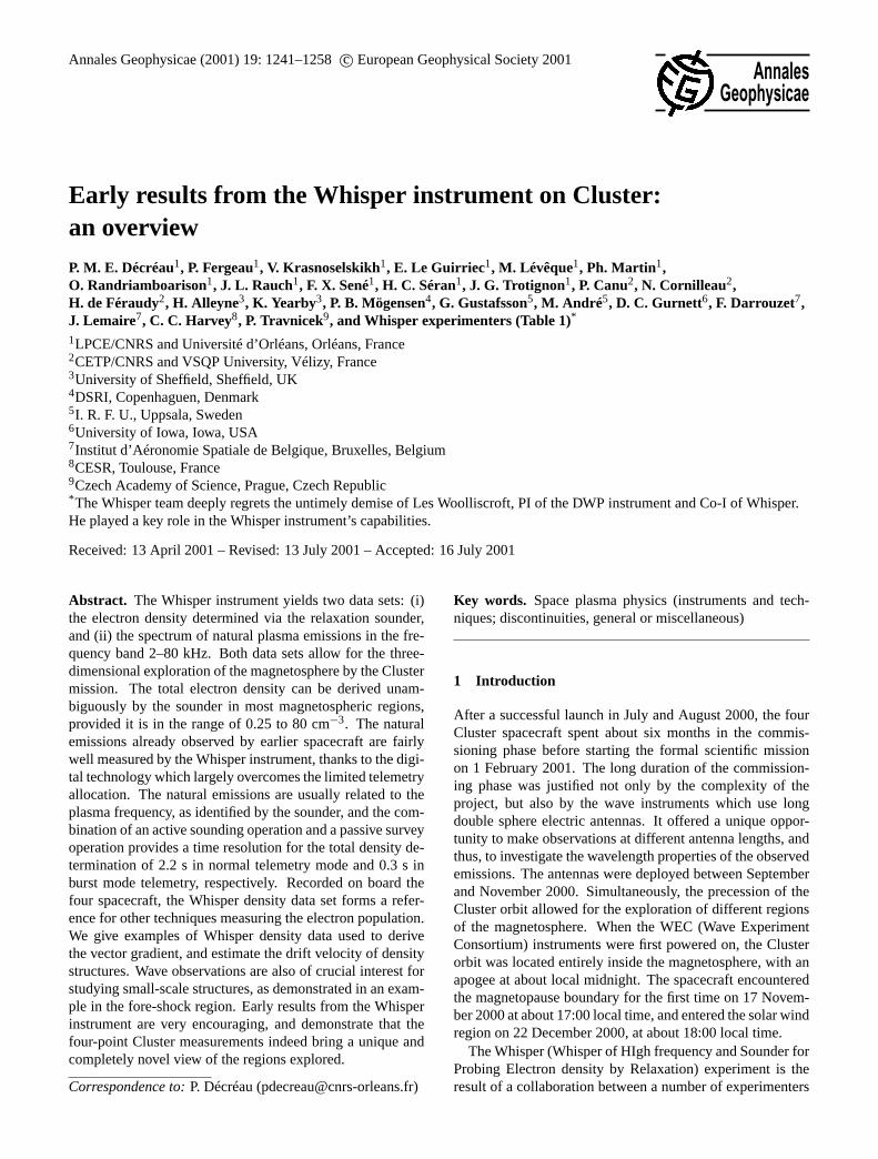
Fig. 4. Frequency/time spectrograms measured on RUMBA (SC1) in the auroral region (two upper panels), and energy and phase angleversus time from spacecraft 1 to 3 (lower panels). The phase angle variations (dotted lines) indicate similar spin periods (from 4.003 to4.017 s). The energy parameter (solid line) is the total energy (in units of potential difference measured by the 88 m dipole) measured inthe 2–80 kHz band. Emissions atFp (about 10 kHz), display a spin modulation peaking along the magnetic field direction. Emissions atFX (about 22 kHz) display unusual spin modulation features present on all four spacecraft (standard Cluster color codes: black, red, green,respectively for spacecraft 1, 2, 3). Spacecraft 4 data, not shown, displays similar features.

with twelve of them in the WEC basic operations. Moreover,the energy parameter product, which can be transmitted at asignificantly higher time resolution (13.3 ms) completes thepicture.

The event presented in Fig. 4, taken in the night side au-roral region (75◦ invariant latitude, 02 MLT, 4.9RE geocen-tric distance), has been chosen to clearly illustrate Whisper’sability to depict spin modulations. In this particular case,the Whisper frequency/time spectrogram from the RUMBAspacecraft (SC1) is presented in the upper panel over a 30

min time interval. This plot shows a narrow band emissionat about 22 kHz, a frequency calledFX hereafter, located be-tween the first and the second harmonic of the electron gyro-frequency (Fce ≈ 14.5 kHz). The emission varies slowlybut surely with time, in both frequency and amplitude. Theelectron gyro-frequencies not associated with any signaturein the natural emissions are revealed by the sounder, whichoperates every 28 s (see Trotignon et al., 2001). The upperhybrid frequencyFuh, observed in the 15–20 kHz band, isalways stimulated by the sounder, associated at times with


03:40 03:48 03:57 04:05 04:13 04:22 04:30 UT

Frequency

(kHz)

40

20

2

40

20

2

RUMBA

SALSA

Fig. 5. Comparison of RUMBA and SALSA frequency/time spectrograms, illustrating several properties of the wave emissions in the internalmagnetosphere on 6 October 2000 (9.5 MLT,−75◦ invariant latitude, 4.3 RE).

strong natural emissions. The middle and lower (three) pan-els of Fig. 4 represent detailed observations during a 35 s timeinterval, including two sounding operations. In the middlepanel, the sounding operations can be recognised by the lim-itation of the individual active spectra to a lowest frequencyof 4 kHz. The three bottom panels display the energy and thephase angle parameters respectively, for spacecraft 1 (blackcurves), spacecraft 2 (red curves) and spacecraft 3 (greencurves), with the periods of sounding operations left blanksince the energy parameter is not available at that time. In-cidentally, this example illustrates the good synchronisationof the operations on the four spacecraft. spacecraft 4 obser-vations, not shown here in order to maintain readability, aresimilar to those of the other Cluster spacecraft.

A striking feature in the detailed plots in Fig. 4 is thefact that theFX emission at about 22 kHz is primarily ap-pearing only at a very specific angle, a few degrees wide inthe spin phase at a quarter of a spin of the overall modu-lation in energy. The overall modulation is associated withthe emission at about 10 kHz which marks the upper rangeof the hiss emissions that are present over almost the entire30 min duration of the event, as shown in the upper panel.After a study of the sounder’s signatures during the completeevent, we could conclude that the emission around 10 kHzcorresponds to the plasma frequency, as the observed patternmatches exactly the relationshipF 2

uh = F 2p + F 2

ce, whereFce

is the recognised electron gyro-frequency, andFuh (the up-per hybrid frequency) is the main resonance triggered by thesounder betweenFce and 2Fce, varying in frequency duringthe event.

The overall modulation of the energy parameter (the sec-ondary wide peak), due to the modulation atFp, resemblesa sinusoidal modulation at twice the spin frequency, as ex-pected for a polarised wave. In order to determine the di-rection of the receiving antenna with respect to the mag-netic field when the energy atFp is maximal, we use the

spacecraft 3 data (green curves), which are particularly cleanaround 00:04 UT. The phase angle of maximumFp energyis about 35◦. Assuming that the spacecraft spin axis is ex-actly along the GSEZ-axis (the directions differ by only afew degrees) and a phase angle of 35◦ is present, this meansthat theYB spacecraft body build axis, located in the spinplane, has rotated through 35◦ since the time it was in theGSEXZ plane (the origin of phase angle). It is thus pointingtoward the morning sector (keeping in mind that the space-craft rotation vector is opposite to that of the Earth). TheEZ

receiving antenna is at 45◦ to YB . In particular, the WEC2sensor (−EZ) is located in the spin plane at a phase angle of10◦ whenYB is at+35◦. The DC magnetic field (GSE com-ponents 441, 92 and 225 nT), projected into the spin plane,corresponds to a phase angle of 12◦. The signal measured atFp is consequently found to be maximal when the receivingantenna is (within the few degrees of uncertainty of the phaseestimation) at its closest alignment with the magnetic field di-rection. Such behaviour is not surprising from a longitudinalLangmuir wave (see, for instance, Thiel and Debrie, 1981,for estimations of signal levels received at different anglesfrom a local dipolar source).

The modulation associated withFX is of a different na-ture. The peculiar, unexpected feature (a narrow peak) ofthe spin modulation seems to indicate some kind of interfer-ence, whereas time variations of the frequency and amplitudefavour interpretation in terms of a natural phenomenon. Suchan interference, if it exists, is not due to another active sci-entific instrument; EDI is off on spacecraft 4, as is ASPOCon spacecraft 1. It does not seem to be related to the EFWsensors, as high resolution EFW products (DC potential dif-ferences) are clean.

The observations from the four spacecraft show similar be-haviour concerning the phase angle of maximalFX emissionaround 00:04 UT: 295◦, 298◦, 306◦ and 285◦ for spacecraft 1to spacecraft 4, respectively, corresponding to phase posi-


tions of the receiving antennas (250◦, 253◦, 261◦ and 240◦)close to perpendicular to the magnetic field direction. How-ever, this fact is purely accidental, as 35 min later, the phaseangle of the maximalFX emission corresponds to an angleof about 27◦ betweenEZ and the magnetic field directionprojected onto the spin plane. On the other hand, the re-ceiving antenna attitude at theFX emission is neither alignedwith the Sun’s direction, nor with a crude estimation of theplasma drift velocity derived from EFW electric field mea-surements. Although we are still far from an interpretationof this unusual event, we would like to point out that theWhisper observational capabilities are at least providing in-teresting clues, which would have been hidden to the formerSFA type of wave instruments.

3 Plasma and wave structures

3.1 Internal magnetosphere

The frequency/time spectrograms obtained from the fourWhisper instruments are usually very rich in information,and a simple visual inspection reveals much about the re-gions crossed. They inform us about two key parameters,the magnetic field strength and the electron density, as seenin the plasma resonance pattern triggered during the sounderoperation (Trotignon et al., 2001). The natural wave emis-sions bring other important clues about the region. They notonly inform us about local plasma conditions, such as theturbulence level in the higher frequency range or the prop-agation characteristics (Canu et al., 2001), but also providea view from a distance of the surrounding region. In somecases, Whisper detects local signatures from transported pop-ulations, informing us about the proximity of their source(an example is shown in Sect. 4.1). In other cases, the wavefeatures observed are due to distant electromagnetic sources,sometimes internal to the magnetosphere, such as a non-thermal continuum or AKR, and sometimes really remote,such as type III solar bursts. The nature of the wave can becharacterised by a comparison of its signatures viewed fromthe different spacecraft; for this, two spacecraft are generallysufficient. An example of wave emissions in the magneto-sphere is shown in Fig. 5. The spacecraft, located over thesouthern hemisphere, are travelling inbound from an auroralregion to the plasmatrough (see Fig. 6, bottom). In the centreof the time interval (04:05 UT), they are located at 75◦ invari-ant latitude, 9.5 MLT and a 4.3 RE geocentric distance. Theinstrument is operated in a Natural Wave mode during thefirst part of the sequence, then from about 04:13 UT it is op-erated, primarily in Sounding mode (a sounder operation canbe recognised by the position at 4 kHz of the low frequencyboundary).

The electron gyro-frequency, around at 20 kHz, indicat-ing a magnetic field amplitude of about 700 nT, is detectedfrom the resonance pattern triggered by the sounder. Thesecond harmonic is sitting at about 40 kHz. The upper hy-brid frequency is observed to increase in time from about 20

-Z

+X 6 Oct. 2000 04:

04:06 04:18 04:30 UT

tS

tR

Fig. 6. Upper panel: density profiles (black for RUMBA, red forSALSA) for a time interval shown in Fig. 5. Lower panel: con-figuration of the 2 spacecraft trajectories (red) and magnetic fieldlines (green) plotted by the OVT visualization tool. Triangles (stan-dard Cluster color-code) show the spacecraft positions at 04:20 UT.The orbit trajectory is almost perpendicular to the field lines, alongwhich we think the density structure is aligned.

to 30 kHz, leading to the density variation shown in Fig. 6(top). These densities are characteristic of magnetic fieldtubes located on the day side that are in the process of beingreplenished from the diurnal ionospheric source (Décréau etal., 1982, Carpenter et al., 1993).

Three types of waves, observed as three different layers,seem to coexist, as is confirmed by two spacecraft observa-tions:

– Observed exactly at the same time on both spacecraft,light blue structured elements are visible above 30 kHz.They are electromagnetic emissions, probably propa-gating non-thermal continuum radiation (Gurnett, 1975;Etcheto et al., 1982). These emissions, homogeneous inspace, are variable with time.

– Wave signatures related to a local density structure,which is apparently stationary with time, but clearly notin space. One signature is the emission at the upperplasma frequency. The strong resonance observed af-ter 04:08 UT, between 20 and 30 kHz in theFce − 2Fce

branch, is interpreted asFuh. It is clearly linked toa natural emission feature present before sounding. Asecond signature, better seen on RUMBA in the centralpart of the plot, is the lower cutoff at about 8 to 12 kHzof the emissions displayed in the orange colour code.Such “trapped continuum radiation" events have been


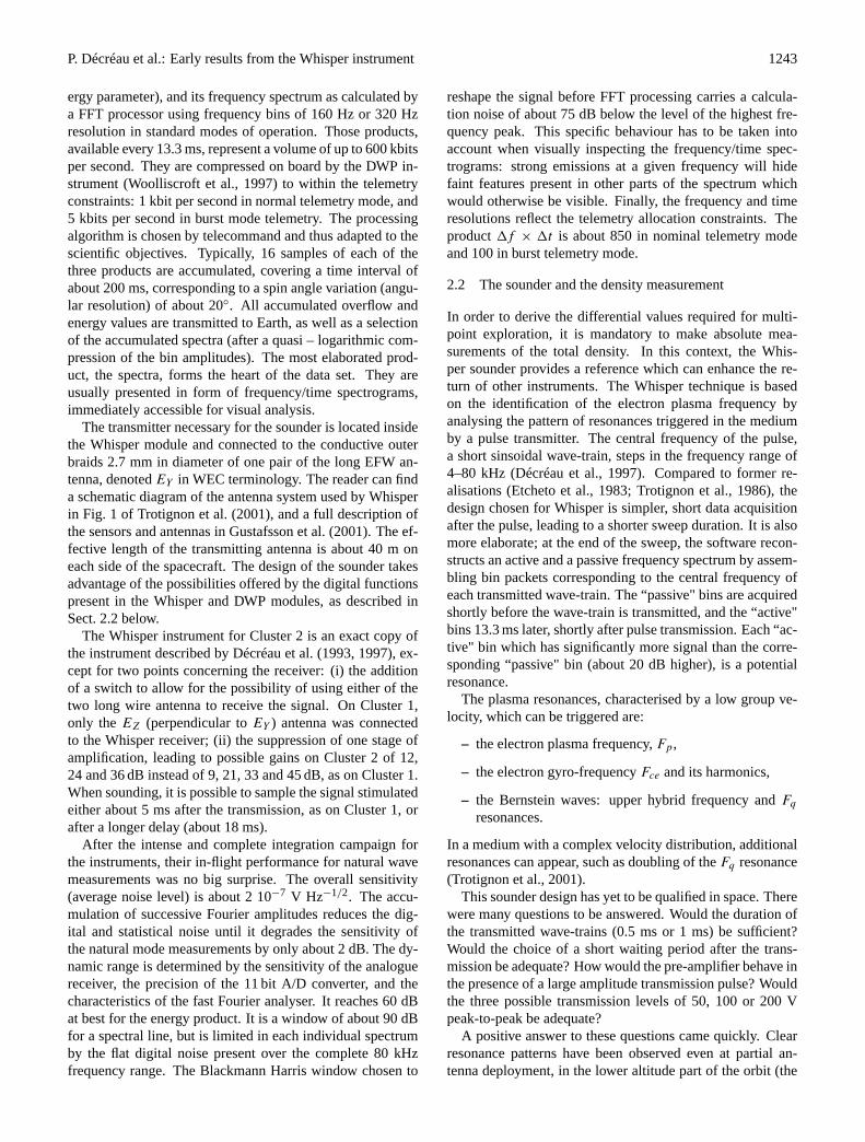
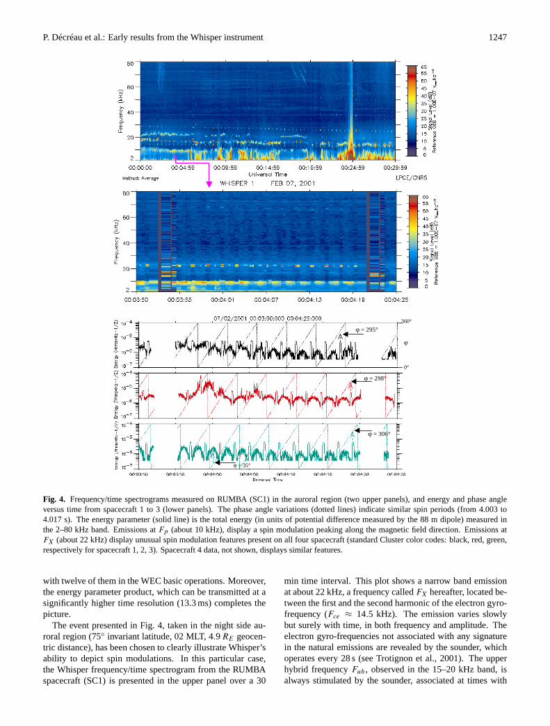
Fig. 7. Frequency/time spectrogram in Sounding only (upper panel) and Natural wave only (bottom panel) modes, derived from TANGO(spacecraft 4) data in the dayside region (11.7 MLT, 81◦ invariant latitude, 8.1RE), outbound leg, on 26 Feb 2001. The sharp density increaseat about 04:06 UT marks the entry in a plasma cloud, left at 05:00 UT, inside the magnetosphere. The magnetopause proper is crossed at06:10 UT.

observed on GEOS or ISEE (Etcheto et al., 1982). Theirlower cutoff frequency is the plasma frequencyFp, asindicated by theFce, Fuh, Fp relationship. Both signa-tures are related to plasma density variations which areobserved first on RUMBA, then on SALSA, but whichlook similar on the two satellites.

– During the first part of the pass, in a dark red colour atthe lowest frequencies of the spectrogram, structures arestable neither in time nor in space (no clear correlationcan be distinguished between RUMBA and SALSA ob-servations). They are intense bursty emissions of a shortduration, interpreted as electrostatic emissions linked towave-particle interactions, known to be active in the au-roral region (Dubouloz et al., 1991).

The density profiles plotted in the upper panel of Fig. 6are similar, with a time delay between SALSA and RUMBA,tS − tR ∼= 205 s, which is almost constant during 20 min ormore. The configuration of the spacecraft orbit and magneticfield line, derived by the Cluster Orbit Visualisation Tool(OVT: see Stasiewicz, 2001) is shown in the lower panel ofFig. 6. The Cluster orbit (red lines) for RUMBA (black sym-bol) and SALSA (red symbol) are almost perpendicular tothe magnetic field lines (green lines), along which we thinkthe density irregularity is aligned. On the other hand, theangle between the orbital velocity vectorV of the constella-tion and the line joining the two satellites is quite low (8◦).Projected along the velocity vector, the spacecraft separationis 1165 km, which when combined with the time delay of

tS − tR, leads to a relative velocity of 5.65 km s−1 betweenthe spacecraft pair and the density structure. This is 10%higher than the spacecraft orbital velocity, implying that thequasi-stationary structure is probably travelling away fromthe Earth at about 0.5 km s−1. The wealth of density data ob-tained from the four spacecraft since the start of the scientificphase of the mission is expected to provide better and morecomplete information about the dynamics of plasma struc-tures in the outer plasmasphere region.

3.2 Plasma structures in the noon sector region

In the noon sector, when travelling outbound from the inter-nal magnetosphere towards the magnetosheath, Cluster of-ten encounters magnetic field tubes loaded with a significantplasma density. The origin of the large plasma bubbles ob-served by Whisper in this region is not obvious. Are thespacecraft crossing a detached plasmaspheric region? Arethey actually crossing the cusp proper, or simply approach-ing this region, in which so many field tubes are converging?

One such event is shown in Fig. 7 from an outbound passin the northern hemisphere. At 04:15 UT, the position isabout 11.7 MLT, 81◦ invariant latitude, at a 8.1RE geocen-tric distance (close to the expected location of the cusp). Thetop panel groups the spectra obtained in Sounding mode, op-erating about twice a minute. The bottom panel groups thespectra obtained in Natural mode at a recurrence of about 3per second. Here, the telemetry rate is in burst mode, whichpermits the highest instrument performance.


SC1SC2SC3SC4

t3 t2 t1 t4

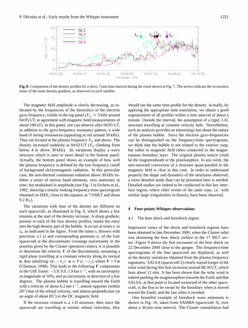
Fig. 8. Comparison of the density profiles for a short, 7 min time interval during the event shown in Fig. 7. The arrows indicate the occurrencetimes of the main density gradient, as observed on each satellite.

The magnetic field amplitude is slowly decreasing, as in-dicated by the frequencies of the harmonics of the electrongyro-frequency, visible in the top panel (Fce ≈ 3 kHz around04:05 UT, in agreement with magnetic field measurements ofabout 100 nT). In this panel, one can observe after 04:05 UT,in addition to the gyro-frequency resonance pattern, a wideband of strong resonances (appearing in red around 30 kHz).They are located at the plasma frequencyFp and above. Thedensity increased suddenly at 04:03 UT (Fp climbing frombelow 4 to above 30 kHz). Its variations display a wavystructure which is seen in more detail in the bottom panel.Actually, the bottom panel shows an example of how wellthe plasma frequency is defined by the low frequency cutoffof background electromagnetic radiation. In this particularcase, the non-thermal continuum radiation above 30 kHz ex-hibits a series of narrow band elements, very stationary intime, but modulated in amplitude (see Fig. 3 in Etcheto et al.,1982, showing a similar looking frequency/time spectrogramobtained on ISEE, close to the equator, at 7.9 MLT and about9.2RE).

The variations with time of the density are different oneach spacecraft, as illustrated in Fig. 8, which shows a fewminutes at the start of the density increase. A sharp gradient,present in each of the four density profiles, marks the entryinto the high density part of the bubble. It occurs at timest1 tot4, as indicated in the figure. From the timesti (known withprecision±1 s) and corresponding positionsr i of the fourspacecraft at the discontinuity crossings (uncertainty in theposition given by the Cluster operation centre), it is possibleto determine the velocityV of the discontinuity, assuming arigid plane travelling at a constant velocity along its normaln, thus satisfying: (r i − rj ) · n = V (ti − tj ), whereV = V n

(Chanteur, 1998). This leads to the followingV componentsin the GSE frame:−5.9, 0.0, 1.9 km s−1, with an uncertaintyin magnitude of 10%, and an uncertainty in direction of a fewdegrees. The plasma bubble is travelling toward the Earthwith a velocity of about 6.2 km s−1, almost opposite (within20◦) that of the orbital velocity, and almost perpendicular (atan angle of about 85◦) to the DC magnetic field.

If the structure crossed is a 1-D structure, then since thespacecraft are travelling at similar orbital velocities, they

should see the same time profile for the density. Actually, byapplying the appropriate time translation, we obtain a goodsuperposition of all profiles within a time interval of about aminute. Outside the interval, the assumption of a rigid, 1-D,structure travelling at constant velocity fails. Nevertheless,such an analysis provides an interesting clue about the natureof the plasma bubble. Since the electron gyro-frequenciescan be distinguished on the frequency/time spectrograms,we think that the bubble is not related to the exterior cusp,but rather to magnetic field tubes connected to the magne-topause boundary layer. The original plasma source couldbe the magnetosheath or the plasmasphere. In any event, theanti-sunward convection of a structure quasi-parallel to themagnetic field is clear in this case. In order to understandproperly the shape and dynamics of the structures observed,a more detailed study than can be presented here is needed.Detailed studies are indeed to be conducted in this key inter-face region, where other events of the same type, i.e. withsimilar large irregularities in density, have been observed.

4 Four-points Whisper observations

4.1 The bow shock and foreshock region

Impressive views of the shock and foreshock regions havebeen obtained in late December 2000, when the Cluster orbitwas skimming the bow shock surface in the 17 MLT sec-tor. Figure 9 shows the first encounter of the bow shock on22 December 2000 close to the apogee. The frequency/timespectrograms of the four spacecraft are displayed, as wellas the density variations obtained from the plasma frequencysignatures. SALSA (spacecraft 2) clearly stayed longer in thesolar wind during this first incursion around 08:30 UT, whichlasts about 12 min. It has been shown that the solar wind isindeed pushing the magnetosphere towards the Earth and thatSALSA, at that point is located westward of the other space-craft, is the first to be swept by the boundary when it movedtoward the Earth, and the last when it receded.

One beautiful example of foreshock wave emissions isshown in Fig. 10, taken from SAMBA (spacecraft 3), overabout a 30 min time interval. The Cluster constellation had


50

20

50

20

(kHz)

50

20

Frequency

50

20

60

40

20

0

SC1

SC3SC2

SC4

RUMBA

SALSA

SAMBA

TANGO

Fig. 9. Frequency/time spectrograms of the four spacecraft during a bow shock crossing (22 December 2000), and the corresponding densityprofiles (bottom panel). The RUMBA (spacecraft 1), SALSA (spacecraft 2), SAMBA (spacecraft 3) and TANGO (spacecraft 4) spacecraftare located at 17:00 LT, close to apogee (12◦ latitude, 19.5RE).

crossed the quasi-perpendicular shock region (as depictedfrom the DC magnetic field configuration), from downstreamto upstream, and entered the electron foreshock. All Clus-ter spacecraft display similar, but not identical, festoon-likefeatures, during about four hours. Such bursty oscillationsaround the plasma frequency have been reported by manyauthors (Anderson et al., 1981; Etcheto and Faucheux, 1984;Fuselier et al., 1985). A characteristic feature of these os-cillations is their intermittent character and their rather largelocal frequency band. Another feature which has given riseto much discussion is the position of their characteristic fre-

quency, which is sometimes well below the local plasma fre-quency. It was found that very near to the electron fore-shock boundary (defined by fast electrons streaming alongmagnetic field lines tangent to the bow shock), the electricfield spectrum occurs in a narrow frequency band centredaround the electron plasma frequency; deeper in the fore-shock region, on shock-connected field lines, the spectrumspreads both upward and downward in frequency (Etchetoand Faucheux, 1984; Fuselier et al., 1985). Whisper, withits specific capabilities, provides a new view of these oscil-lations. In Fig. 10, the upper panel presents the Whisper fre-


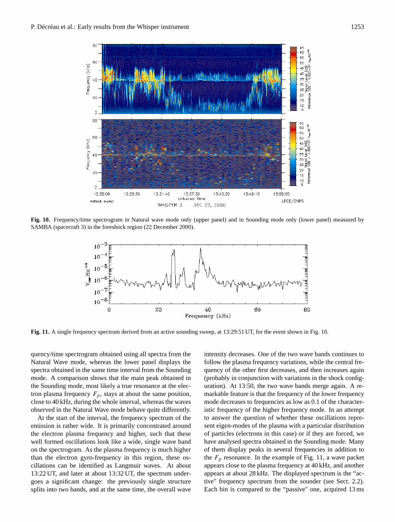
Fig. 10. Frequency/time spectrogram in Natural wave mode only (upper panel) and in Sounding mode only (lower panel) measured bySAMBA (spacecraft 3) in the foreshock region (22 December 2000).

Fig. 11. A single frequency spectrum derived from an active sounding sweep, at 13:29:51 UT, for the event shown in Fig. 10.

quency/time spectrogram obtained using all spectra from theNatural Wave mode, whereas the lower panel displays thespectra obtained in the same time interval from the Soundingmode. A comparison shows that the main peak obtained inthe Sounding mode, most likely a true resonance at the elec-tron plasma frequencyFp, stays at about the same position,close to 40 kHz, during the whole interval, whereas the wavesobserved in the Natural Wave mode behave quite differently.

At the start of the interval, the frequency spectrum of theemission is rather wide. It is primarily concentrated aroundthe electron plasma frequency and higher, such that thesewell formed oscillations look like a wide, single wave bandon the spectrogram. As the plasma frequency is much higherthan the electron gyro-frequency in this region, these os-cillations can be identified as Langmuir waves. At about13:22 UT, and later at about 13:32 UT, the spectrum under-goes a significant change: the previously single structuresplits into two bands, and at the same time, the overall wave

intensity decreases. One of the two wave bands continues tofollow the plasma frequency variations, while the central fre-quency of the other first decreases, and then increases again(probably in conjunction with variations in the shock config-uration). At 13:50, the two wave bands merge again. A re-markable feature is that the frequency of the lower frequencymode decreases to frequencies as low as 0.1 of the character-istic frequency of the higher frequency mode. In an attemptto answer the question of whether these oscillations repre-sent eigen-modes of the plasma with a particular distributionof particles (electrons in this case) or if they are forced, wehave analysed spectra obtained in the Sounding mode. Manyof them display peaks in several frequencies in addition totheFp resonance. In the example of Fig. 11, a wave packetappears close to the plasma frequency at 40 kHz, and anotherappears at about 28 kHz. The displayed spectrum is the “ac-tive" frequency spectrum from the sounder (see Sect. 2.2).Each bin is compared to the “passive" one, acquired 13 ms


ω / ωpe

2.0

1.5

1.0

0.5

0.0

kλ

0.0 0.1 0.2 0.3 0.4 0.5 0.6

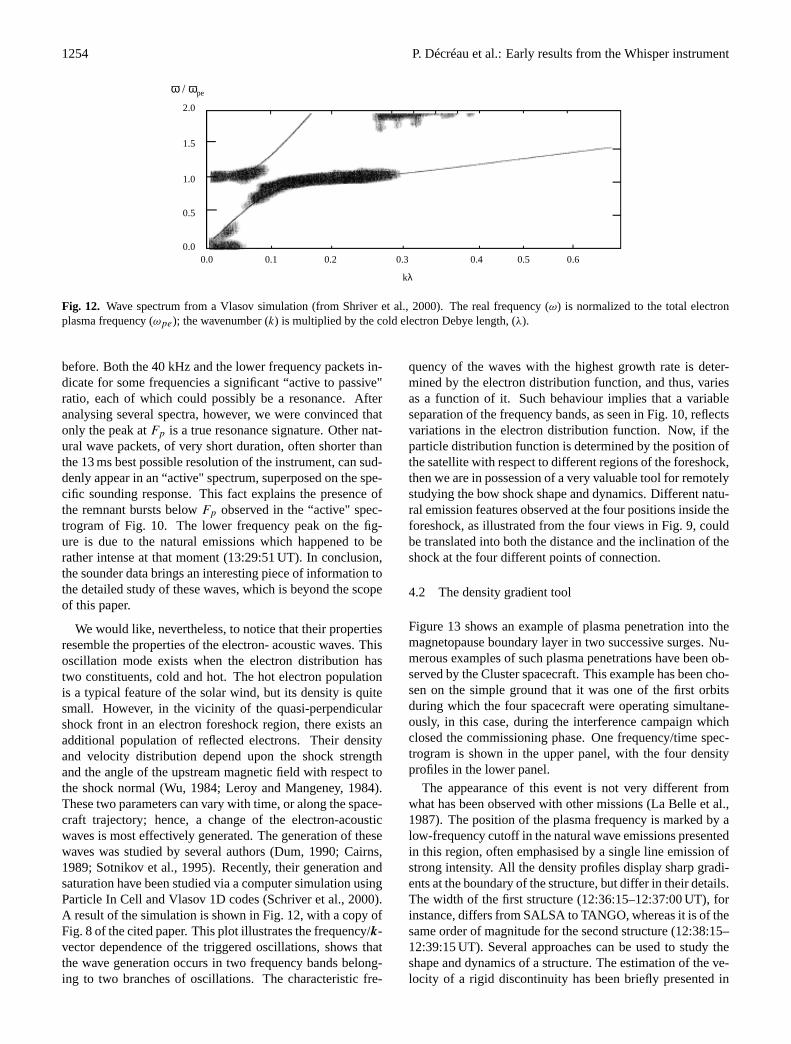
Fig. 12. Wave spectrum from a Vlasov simulation (from Shriver et al., 2000). The real frequency (ω) is normalized to the total electronplasma frequency (ωpe); the wavenumber (k) is multiplied by the cold electron Debye length, (λ).

before. Both the 40 kHz and the lower frequency packets in-dicate for some frequencies a significant “active to passive"ratio, each of which could possibly be a resonance. Afteranalysing several spectra, however, we were convinced thatonly the peak atFp is a true resonance signature. Other nat-ural wave packets, of very short duration, often shorter thanthe 13 ms best possible resolution of the instrument, can sud-denly appear in an “active" spectrum, superposed on the spe-cific sounding response. This fact explains the presence ofthe remnant bursts belowFp observed in the “active" spec-trogram of Fig. 10. The lower frequency peak on the fig-ure is due to the natural emissions which happened to berather intense at that moment (13:29:51 UT). In conclusion,the sounder data brings an interesting piece of information tothe detailed study of these waves, which is beyond the scopeof this paper.

We would like, nevertheless, to notice that their propertiesresemble the properties of the electronacoustic waves. Thisoscillation mode exists when the electron distribution hastwo constituents, cold and hot. The hot electron populationis a typical feature of the solar wind, but its density is quitesmall. However, in the vicinity of the quasi-perpendicularshock front in an electron foreshock region, there exists anadditional population of reflected electrons. Their densityand velocity distribution depend upon the shock strengthand the angle of the upstream magnetic field with respect tothe shock normal (Wu, 1984; Leroy and Mangeney, 1984).These two parameters can vary with time, or along the space-craft trajectory; hence, a change of the electron-acousticwaves is most effectively generated. The generation of thesewaves was studied by several authors (Dum, 1990; Cairns,1989; Sotnikov et al., 1995). Recently, their generation andsaturation have been studied via a computer simulation usingParticle In Cell and Vlasov 1D codes (Schriver et al., 2000).A result of the simulation is shown in Fig. 12, with a copy ofFig. 8 of the cited paper. This plot illustrates the frequency/k-vector dependence of the triggered oscillations, shows thatthe wave generation occurs in two frequency bands belong-ing to two branches of oscillations. The characteristic fre-

quency of the waves with the highest growth rate is deter-mined by the electron distribution function, and thus, variesas a function of it. Such behaviour implies that a variableseparation of the frequency bands, as seen in Fig. 10, reflectsvariations in the electron distribution function. Now, if theparticle distribution function is determined by the position ofthe satellite with respect to different regions of the foreshock,then we are in possession of a very valuable tool for remotelystudying the bow shock shape and dynamics. Different natu-ral emission features observed at the four positions inside theforeshock, as illustrated from the four views in Fig. 9, couldbe translated into both the distance and the inclination of theshock at the four different points of connection.

4.2 The density gradient tool

Figure 13 shows an example of plasma penetration into themagnetopause boundary layer in two successive surges. Nu-merous examples of such plasma penetrations have been ob-served by the Cluster spacecraft. This example has been cho-sen on the simple ground that it was one of the first orbitsduring which the four spacecraft were operating simultane-ously, in this case, during the interference campaign whichclosed the commissioning phase. One frequency/time spec-trogram is shown in the upper panel, with the four densityprofiles in the lower panel.

The appearance of this event is not very different fromwhat has been observed with other missions (La Belle et al.,1987). The position of the plasma frequency is marked by alow-frequency cutoff in the natural wave emissions presentedin this region, often emphasised by a single line emission ofstrong intensity. All the density profiles display sharp gradi-ents at the boundary of the structure, but differ in their details.The width of the first structure (12:36:15–12:37:00 UT), forinstance, differs from SALSA to TANGO, whereas it is of thesame order of magnitude for the second structure (12:38:15–12:39:15 UT). Several approaches can be used to study theshape and dynamics of a structure. The estimation of the ve-locity of a rigid discontinuity has been briefly presented in


0,0

0,5

1,0

1,5

2,0

2,5

3,0

3,5

4,0

4,5

5,0

12:35:00 12:36:00 12:37:00 12:38:00 12:39:00 12:40:00

Time [UT]

Den

sity

[cm

-3]

RUMBA/SC1SALSA/SC2SAMBA/SC3TANGO/SC4

2

10

20

30

40

Fre

qu

ency

[kH

z]

SALSA/SC2

WHISPER/CLUSTER 12 Dec. 2000

Fig. 13. Two successive plasma transfer events in the magnetopause boundary layer (17 MLT, 28◦ latitude, 17.2RE). The bottom panelshows the density profiles derived from the four frequency/time spectrograms analogous to the one in the upper panel.

an example in Sect. 3.2. We wish to present now anotherapproach, namely the derivation of the density gradient vec-tor, using data of the event presented in Fig. 13. The conceptis simple: four values of a given parameter, here the scalardensity, taken at the same time at four known positions, willprovide an estimation of the density gradient vector. The es-timation will be representative only if the gradient is actuallyconstant inside the tetrahedron volume, a condition that can-not be tested in a simple way. Our aim here is to give a briefsummary of the method used in practice, and present resultsobtained with the gradient tool, rather than discussing its va-lidity in detail.

The least square method of determining the spatial gra-dient of a parameter using data acquired simultaneouslyfrom four (or more) spacecraft has been described by Har-vey (1998). It turns out that the spatial gradient can be ex-pressed in terms of the inverse of a symmetric tensor formedfrom the relative positions of the spacecraft. In the specialcase of four spacecraft, this tensor is referred to as the vol-umetric tensor (its determinant is (3V/8)2, whereV is thevolume of the tetrahedron). The tensor is

Rij =1

4

4∑α=1

(r iα − r i

b

) (rjα − r

jb

),

wherer iα andr

jα are the three coordinates of the position of

the spacecraftα (α = 1, 2, 3 or 4), andr ib are the coordinates

of the position of the centre of mass of the four spacecraft.The volumetric tensor describes basic geometrical properties

of the tetrahedron defined by the four spacecraft. The eigen-values can be used to define the characteristic sizeL, theelongationE and the planarityP , and the eigenvectors de-fine the directions of elongationeE and planarityeP (Robertet al., 1998). In terms of these geometrical parameters, whichare included in the Summary Parameters of the Cluster Sci-entific Data System, the inverse of the volumetric tensor maybe expressed as:

R−1ji =

4

L2[eEj

eEi +1

(1 − E)2eLj eLj +

1

(1 − P )2(1 − E)2ePj eP i

],

whereeL is the third, mutually orthogonal direction,eL =

eP xeE . Finally, it can be shown that the least squares esti-mation (which for four spacecraft, is, in fact, the exact esti-mation) of the linear density gradient is:

δn

δri=

1

2

1

42

∑j

[4∑

α=1

4∑β=1

(nα − nβ)(rjα − r

jβ)

]× R−1

ji ,

wherenα is the value of densityn measured on the spacecraftα.

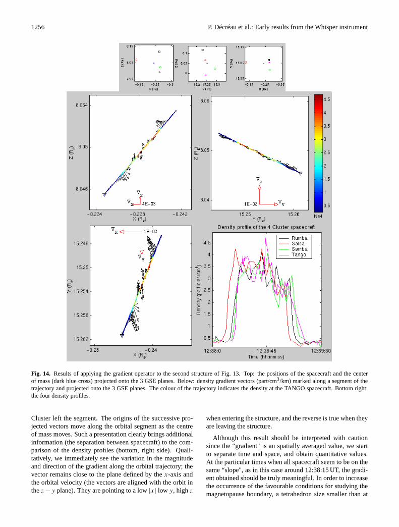
The density gradient vectors obtained during the crossingof the second structure are shown in Fig. 14. The succes-sive values determined are displayed, projected onto the threeplanes of the GSE coordinate system. The orbital segmentof the centre of mass of the constellation is also projectedonto each plane, with a triangle to indicate the point at which


Fig. 14. Results of applying the gradient operator to the second structure of Fig. 13. Top: the positions of the spacecraft and the centerof mass (dark blue cross) projected onto the 3 GSE planes. Below: density gradient vectors (part/cm3/km) marked along a segment of thetrajectory and projected onto the 3 GSE planes. The colour of the trajectory indicates the density at the TANGO spacecraft. Bottom right:the four density profiles.

Cluster left the segment. The origins of the successive pro-jected vectors move along the orbital segment as the centreof mass moves. Such a presentation clearly brings additionalinformation (the separation between spacecraft) to the com-parison of the density profiles (bottom, right side). Quali-tatively, we immediately see the variation in the magnitudeand direction of the gradient along the orbital trajectory; thevector remains close to the plane defined by thex-axis andthe orbital velocity (the vectors are aligned with the orbit inthez − y plane). They are pointing to a low|x| low y, highz

when entering the structure, and the reverse is true when theyare leaving the structure.

Although this result should be interpreted with cautionsince the “gradient" is an spatially averaged value, we startto separate time and space, and obtain quantitative values.At the particular times when all spacecraft seem to be on thesame “slope", as in this case around 12:38:15 UT, the gradi-ent obtained should be truly meaningful. In order to increasethe occurrence of the favourable conditions for studying themagnetopause boundary, a tetrahedron size smaller than at


the start of the mission has to be considered. This situationis foreseen to take place in late 2001 (100 km spacecraft sep-aration, to be compared to 600 km in December 2000).

5 Summary and conclusion

In summary, the first observations from the Whisper instru-ment on Cluster are startling. The instrument’s receiver andwave analyser behave beautifully, and the technology, whichwas chosen almost twelve years ago, proves the existence ofnew capabilities, such as the possibility of measuring wavedirectivity. The sensitivity and the time/frequency resolutionare able to show small differences between the four space-craft, which is the main objective.

Whisper’s sounder design proved to be efficient in the vastmajority of the cases encountered. The main limitations,which have not yet been fully investigated, are inherent tothe technique: the density is derived indirectly, and the reso-nance recognition process is not 100% efficient, especially incomplex plasmas; and simple instrument limitations excludesome regions or some plasma regimes.

The exploration of regions that are not yet well-known hasproven to be fascinating, from plasmapause regions to thesolar wind, including the magnetosheath and cusp regions,which sometimes look different from what is described inthe text books. The examples shown in this paper are onlysome of the events which can be studied using Whisper data.WC have now to put together the different pieces of informa-tion, to compare instruments, to test the multi-point analysistechniques which have been prepared, and imagine new onesbased on real data. A difficult but fascinating challenge isahead.

Acknowledgements.The authors wish to acknowledge the effortsof a number of people who, at one time or another, worked for theWHISPER experiment: A. Bahnsen, from DSRI, A. Sumner, C.Dunford, J. Thompson (Univ. Sheffield); C. Vasiljevic, E. Guyot,L. Launay, J.-L. Fousset, (LPCE). The WEC, ESA, Dornier, RALand IABG teams are warmly thanked for their participation and helpin the testing and integration of the experiment. Our warm thankstoo to engineers at Starsem and ESOC for a faultless launch, and tothe JSOC and ESOC teams for supporting complex operations. Weare grateful to G. Chanteur (CETP, Vélizy), who derived the valueof a discontinuity velocity and associated uncertainties. Several dis-cussions have benefited from the availability of magnetometer data(courtesy of A. Balogh), and we express our thanks to the FGMteam. We wish to extend our thanks to those who helped the WHIS-PER investigators in their contribution to the CSDS, in particular J.-P. Thouvenin, H. Poussin, M. Nonon, J.-Y. Prado and J.-C. Kosik ofCNES. The WHISPER experiment and software are realised thanksto a CNES contract. The transmitter hardware was designed andbuilt at DSRI.

Topical Editor M. Lester thanks H. Laakso and another refereefor their help in evaluating this paper.

References

Anderson, R. R., Parks, G. K., Eastman, T. E., Gurnett, D. A., andFrank, L. A.: Plasma waves associated with energetic particlesstreaming into the solar wind from the Earth’s bow shock, J. Geo-phys. Res., 86, 4493–4510, 1981.

Béghin, C. and Kolesnikova, E.: Surface-charge distribution ap-proach for modeling of quasi-static electric antennas in isotropicthermal plasma, Radio Sci., 33, 503–516, 1998.

Cairns, I.: Electrostatic wave generation above and below theplasma frequency by electron beams, Phys. Fluids, B1, 204–213,1989.

Canu, P., Décréau, P. M. E., Trotignon, J. G., Rauch, J. L., Séran, H.C., Fergeau, P., Lévêque, M., Martin, Ph., Sené, F. X., Le Guir-riec, E., Alleyne, H., and Yeraby, K.: Identification of naturalplasma emissions with the Cluster – Whisper relaxation sounder,Ann. Geophysicae, this issue, 2001.

Carpenter, D. L., Giles, B. L., Chappell, C. R., Décréau, P. M. E.,Anderson, R. R., Persoon, A. M., Smith, A. J., Corcuff, Y., andCanu, P.: Plasmasphere dynamics in the duskside bulge region:a new look at an old topic, J. Geophys. Res., 98, 19, 243–271,1993.

Chanteur, G.: Spatial interpolation for four spacecraft: Theory, in:Analysis methods for Multi-Spacecraft data, (Eds) Paschmann,G. and Daly, P. W., ISSI scientific Report SR-001, 349–369,1998.

Décréau, P. M. E., Fergeau, P., Lévêque, M., Martin, Ph., Ran-driamboarison, O., Sené, F. X., Trotignon, J. G., Canu, P., deFéraudy, H., Bahnsen, A., Jespersen, M., Mögensen, P. B.,Iversen, I., Dunford, C., Sumner, A., Woolliscroft, L. J. C.,Gustafsson, G., and Gurnett, D. A.: “Whisper", a sounder andHigh frequency wave analyser experiment, ESA SP-1159, 51–67, 1993.

Décréau, P. M. E., Fergeau, P., Krasnoselskikh, V., Lévêque, M.,Martin, Ph., Randriamboarison, O., Sené, F. X., Trotignon, J. G.,Canu, P., Mögensen, P. B. and Whisper investigators: Whisper,a resonance sounder and wave analyser: performances and per-spectives for the Cluster mission, Space Sci. Rev., 79, 93–105,1997.

Décréau, P. M. E., Béghin, C., and Parrot, M.: Global characteris-tics of the cold plasma in the equatorial plasmapause region asdeduced from the GEOS 1 mutual impedance probe, J. Geophys.Res., 87, 695–712, 1982.

Dubouloz, N., Pottelette, R., Malingre, M., Holmgren, G., andLindqvist, P. A.: Detailed analysis of broadband electrostaticnoise in the dayside auroral zone, J. Geophys. Res., 96, 3565–3579, 1991.

Dum, C. T.: Simulation of Plasma Waves in the Electron Foreshock:The Generation of Downshifted Oscillations, J. Geophys. Res.,95, 8123–8131, 1990.

Etcheto, J., Christiansen, P. J., Gough, M. P., and Trotignon, J. G.:Terrestrial Continuum radiation observations with GEOS-1 andISEE-1, Geophys. Res. Let., 9, 1239–1242, 1982.

Etcheto, J., Belmont, G., Canu, P., and Trotignon, J. G.: Activesounder experiments on GEOS and ISEE, ESA SP6195, 39–46,1983.

Etcheto, J. and Faucheux, M.: Detailed study of electron plasmawaves upstream of the Earth’s bow shock, J. Geophys. Res., 89,6631–6653, 1984.

Fuselier, S. A., Gurnett, D. A., and Fitzenreiter, R. J.: The downshiftof electron plasma oscillations in the electron foreshock region,J. Geophys. Res., 90, 3935–3946, 1985.


Gurnett, D. A.: The Earth as a radio source: the nonthermal contin-uum, J. Geophys.Res. 80, 2751–2763, 1975.

Gustafsson, G., Boström, R., Holback, B., Holmgren, G., Lundgren,A., Stasiewicz, K., Ahlen, L., Mozer, F. S., Pankow, D., Harvey,P., Berg, P., Ulrich, R., Pedersen, A., Schmidt, R., Butler, A.,Fransen, A. W. C., Klinge, D., Thomsen, M., Fälthammar, C.-G.,Lindqvist, P.-A., Christenson, S., Holtet, J., Lybekk, B., Sten, T.A., Tanskanen, P., Lappalainen, K., and Wygant, J.: The electricfiled and wave experiment for the Cluster mission, Space Sci.Rev., 79, 137–156, 1997.

Gustafsson, G., André, M., Carozzi, T., Eriksson, A. I., Fältham-mar, C.-G., Grard, R., Holmgren, G., Holtet, J. A., Ivchenko,N., Karlsson, T., Khotyaintsev, Y., Klimov, S., Laakso, H.,Lindqvist, P.-A., Lybekk, B., Marklund, G., Mozer, F., Mur-sula, K., Pedersen, A., Popielawska, B., Savin, S., Stasiewicz,K., Tanskanen, P., Vaivads, A., and Wahlund, J.-E.: First resultsof electric field and density observations by Cluster EFW basedon initial months of observations, Ann. Geophyicae, this issue,2001.

Harvey, C. C.: Spatial gradient and the volumetric tensor, in: Anal-ysis methods for Multi-Spacecraft data, (Eds) Paschmann, G. andDaly, P. W., ISSI scientific Report SR-001, pp. 307–322, 1998.

Hulqvist, B.: The Viking project, Geophys. Res. Let. 74, 379–382,1987.

LaBelle, J., Treumann, R. A., Haerendel, G., Bauer, O. H.,Paschmann, G., Baumjohan, W., Lühr, H., Anderson, R. R.,Koons, H. C., and Holzworth, R. H.: AMPTE-IRM observa-tions of waves associated with flux transfer events in the mag-netosphere, J. Geophys. Res., 92, 5827–5843, 1987.

Leroy, M. M. and Mangeney, A.: A theory of energization of solarwind electrons by the Earth’s bow shock, Ann. Geophysicae, 2,440–456, 1984.

Meyer-Vernet, N. and Perche, C.: Tool kit for antennae and thermalnoise near the plasma frequency, J. Geophys. Res., 94, 2401–2415, 1989.

Pedersen, A., Cornilleau-Wherlin, N., De La Porte, B., Roux, A.,Bouabdellah, A., Décréau, P. M. E., Lefeuvre, F., Sené, F. X.,Gurnett, D., Huff, R., Gustafsson, G., Holmgren, G., Woollis-croft, L., Alleyne, H. St. C., Thompson, J. A., and Davies, P. N.

H.: The Wave Experiment Consortium (WEC), Space Sci. Rev.,79, 157–193, 1997.

Robert, P., Roux, A., Harvey, C. C., Dunlop, M. W., Daly, P. W., andGlassmeier, K.-H.: Tetrahedron Geometric Factors, in: Analy-sis methods for Multi-Spacecraft data, (Eds) Paschmann, G. andDaly, P. W., ISSI scientific Report SR-001, 323–348, 1998.

Schriver, D., Ashour-Abdalla, M., Sotnikov, V., Hellinger, P., Fi-ala, V., Bingham, R., and Mangeney, A.: Excitation of electronacoustic waves near the electron plasma frequency and at twicethe plasma frequency, J. Geophys. Res., 105, 12, 919–927, 2000.

Sotnikov, V. I., Schriver, D., Ashour-Abdalla, M., Ernstmeyer, J.,and Myers, N.: Excitation of electron acoustic waves by a gyrat-ing electron beam, J. Geophys. Res., 100, 19, 765–772, 1995.

Stasiewicz, K.: OVT Visualization Tool-2 for CLUSTER, UserGuide, Copyright c©2000 by the OVT team, version 2.0,http://ovt.irfu.se, 2001.

Thiel, J. and Debrie, R.: Electrostatic wave potential at the plasmaand upper-hybrid resonances, J. Plasma Phys., 25, 239–254,1981.

Trotignon, J. G., Etcheto, J., and Thouvenin, J. P., Automatic de-termination of the electron density measured by the relaxationsounder on-board ISEE 1, J. Geophys. Res. 91, 4302–4320,1986.

Trotignon J. G., Décréau, P. M. E., Rauch, J. L., Randriamboarison,O., Krasnoselskikh, V., Canu, P., Alleyne, H., Yeraby, K., LeGuirriec, E., Séran, H. C., Sené, F. X., Martin, Ph., Lévêque, M.,and Fergeau, P.: How to determine the thermal electron densityand the magnetic field strength from the CLUSTER/WHISPERobservations around the Earth, Ann. Geophysicae, this issue,2001.

Woolliscroft, L. J. C., Alleyne, H. ST. C., Dunford, C. M., Sumner,A., Thompson, J. A., Walker, S. N., Yearby, K. H., Buckley, A.,Chapman, S., Gough, P., and the DWP investigators: The Digi-tal Wave-Processing experiment on Cluster, Space Sci. Rev., 79,209–231, 1997.

Wu, C. S.: A fast Fermi process: energetic electrons accelerated bya nearly perpendicular Bow Shock, J. Geophys. Res., 89, 8857–8862, 1984.

early results from the whisper instrument on cluster ... · early results from the whisper...

Documents