1

Early results from the Whisper instrument on CLUSTER: an overview

P.M.E. Décréau, P. Fergeau, V. Krasnoselskikh, E. Le Guirriec, M. Lévêque , Ph. Martin,

O. Randriamboarison, J. L. Rauch, F.X. Sené, H.C. Séran, J. G. Trotignon, LPCE/CNRS and Université d’Orléans, Orléans, France,

P. Canu, N. Cornilleau, H. de Féraudy, CETP/CNRS and VSQP University, Vélizy, France H. Alleyne, K. Yearby, University of Sheffield, Sheffield, U.K.

P. B. Mögensen, DSRI, Copenhaguen, Denmark G. Gustafsson, M. André, I.R.F.U., Uppsala, Sweden

D. C. Gurnett, University of Iowa, Iowa, U.S.A F. Darrouzet, J. Lemaire, Institut d’Aéronomie Spatiale de Belgique, Bruxelles, Belgique

C.C. Harvey, CESR, Toulouse, France P. Travnicek, Czech Acad. Sci., Prague, Czech Republic

and Whisper experimenters (Table 1)*

Abstract

The Whisper instrument yields two data sets : (i) the electron density determined via the relaxation sounder, and (ii) the spectrum of natural plasma emissions in the frequency band 2−80 kHz. Both data sets allow three dimensional exploration of the magnetosphere by the Cluster mission. The total electron density can be derived unambiguously by the sounder in most magnetospheric regions, provided it is in the range 0.25 to 80 cm-3. The natural emissions already observed by earlier spacecraft are fairly well measured by the Whisper instrument, thanks to the digital technology which largely overcomes the limited telemetry allocation. The natural emissions are usually related to the plasma frequency as identified by the sounder, and the combination of active sounding operation and passive survey operation allows a time resolution for the total density determination of respectively 2.2 s in normal telemetry mode and 0.3 s in burst mode telemetry. Recorded aboard the four spacecraft, the Whisper density data set forms a reference for other techniques measuring the electron population. We give examples of Whisper density data used to derive the vector gradient, and estimate the drift velocity of density structures. Wave observations are also of crucial interest for studying small scale structures, as demonstrated in an example in the fore-shock region. Early results from the Whisper instrument are very encouraging, and demonstrate that the four-point Cluster measurements indeed bring a unique and completely novel view of the regions explored. Keywords: 7894 (Instruments and techniques), 7811 (Discontinuities), 7899 (General or miscellaneous) * The Whisper team deeply regrets the untimely demise of Les Woolliscroft, PI of the DWP instrument and Co-I of Whisper. He played a key role in making the Whisper instrument what it is. Contact for editorial matters : Pierrette Décréau E-mail: pdecreau@cnrs-orleans.fr Phone: (33) 2 38 25 52 64, Fax: (33) 2 63 12 Laboratoire de Physique et Chimie de l’Environnement, CNRS, 3A Avenue de la Recherche Scientifique, F-45071 Orléans Cédex 02, France

2

1. Introduction

After a successful launch in July and August 2000, the four Cluster spacecraft spent about six months

in the commissioning phase of before starting the formal scientific mission on 1st February 2001. The

long duration of the commissioning phase was justified not only by the complexity of the project but

also by the wave instruments which use long double sphere electric antennas, because it offered a

unique opportunity to make observations at different antenna lengths, and thus investigate the

wavelength properties of the observed emissions. The antennas were deployed between September and

November 2000. Simultaneously, the precession of the Cluster orbit allowed exploration of different

regions of the magnetosphere. When the WEC (Wave Experiment Consortium) instruments were first

powered on, the Cluster orbit was located entirely inside the magnetosphere, with an apogee at about

local midnight. The spacecraft encountered the magnetopause boundary first time in November 17

2000 at about 17:00 local time, and entered the solar wind region in December 22 2000, at about 18:00

local time.

The Whisper (Whisper of HIgh frequency and Sounder for Probing Electron density by Relaxation)

experiment is the result of collaboration between a number of experimenters (Table 1), organised

within the context of the Wave Experiment Consortium, which groups five instruments (Pedersen et

al., 1997). The Whisper instrument consists basically of a receiver, a transmitter, and a wave spectrum

analyser, completed by the sensors of EFW (Electric Field Wave experiment), and functions of DWP

(Digital Wave Processing experiment), two other WEC instruments. Whisper is devoted to the survey,

active and passive, of the WEC electric signal in the high frequency range from about 2 to 80 kHz,

which includes electrostatic and electromagnetic natural emissions of interest to the Cluster objectives.

It includes emissions in the vicinity of the plasma frequency, essential for density diagnosis, one of the

main functions of the Whisper experiment.

The purpose of this paper is to describe the in-flight performance of the Whisper instrument and

present examples of data acquired during the early phase of the mission.

We emphasise two aspects of the early phase of the Cluster mission: the progressive use of operational

capabilities on one hand, the unveiling of hidden views of the magnetosphere on the other hand. The

observations collected so far by the four instruments are so rich that it is impossible to present a

complete overview of their content, and many interesting features will not be shown or even

mentioned here. Instead, we aim to give, via a few selected examples, an idea both of the intrinsic

performance of Whisper and of characteristics, as revealed by the four-point measurements, of some

of the magnetospheric structures encountered.

3

The paper is organised in three main sections. Section 2 illustrates the operation and performance of

each individual instrument, in particular the articulation between its two modes of operation: the

sounder, measuring the absolute electron density, and the wave spectrum analyser. Section 3 presents

examples of plasma or wave structures observed in different regions of the magnetosphere, and

estimations of the drift velocity of density structures. In section 4, we present two examples of four

points observations, and discuss the derivation of the density gradient vector. A brief summary closes

the paper.

2. The Whisper instrument in flight

2.1 General design

The design of the Whisper instrument has benefited from experience gained with magnetospheric

sounders realised in the seventies or eighties (GEOS 1 and 2, ISEE 1, and Viking missions), but its

technical realisation is rather different. Consequently its performance is different, and some of the

wave features seen in frequency/time spectrograms may look somewhat different.

The design, operational features and performance are described in detail by Décréau et al. [1993,

1997]. The electric signals from the four sensors of the EFW instrument (Gustafsson et al., 1997,

2001), that is, from the high impedance amplifiers located in the vicinity of the spheres, are high-pass

filtered and fed to the Whisper module where signal from two opposite sensors enter differential

amplifiers so as to yield effectively one of the two long (88 m tip to tip) double sphere dipoles. The

Whisper receiver consists of a gain amplifier and filters isolating the 2 – 80 kHz band, and an 11 bits

Analogue to Digital (A/D) converter. The digital signal is used by the Whisper analyser module and

controller to generate three products: the number of overflows counted during the acquisition intervals

(a few milliseconds every 13.3 ms), the total energy of the waveform signal (referred to as the Energy

parameter), and its frequency spectrum as calculated by a FFT processor using frequency bins of

160 Hz or 320 Hz resolution in standard modes of operation. Those products, available every 13.3 ms,

represent a volume of up to 600 kbits per second. They are compressed on board by the DWP

instrument (L.J.C. Woolliscroft et al., 1997) to within the telemetry constraints: 1 kbits per second in

normal telemetry mode, and 5 kbits per second in burst mode telemetry. The processing algorithm is

chosen by telecommand and thus adapted to the scientific objectives. Typically, 16 samples of each of

the three products are accumulated, covering a time interval of about 200 ms, corresponding to a spin

angle variation (angular resolution) of about 20 degrees. All accumulated overflow and energy values

are transmitted to ground, as well as a selection of the accumulated spectra (after a quasi - logarithmic

compression of the bin amplitudes). The most elaborated product, the spectra, forms the heart of the

4

data set. They are usually presented in form of frequency/time spectrograms, immediately accessible

for visual analysis.

The transmitter necessary for the sounder is located inside the Whisper module and connected to the

conductive outer braids, 2.7 mm in diameter, of one pair of the long EFW antenna, denoted Ey in

WEC terminology. The reader can find a schematic diagram of the antenna system used by Whisper

in Figure 1 of Trotignon et al., (2001), and a full description of the sensors and antennas in Gustafsson

et al., (2001). The effective length of the transmitting antenna is of about 40 m on each side of the

spacecraft. The design of the sounder takes advantage of the possibilities offered by the digital

functions present in the Whisper and DWP modules, as described in section 2.2 below.

The Whisper instrument for Cluster 2 is an exact copy of the instrument described by Décréau et al.

[1993,1997], except for two points concerning the receiver: (i), addition of a switch to allow the

possibility of using either of the two long wire antenna to receive the signal – on Cluster 1, only the Ez

(perpendicular to Ey) antenna was connected to the Whisper receiver, (ii), suppression of one stage of

amplification, leading on Cluster 2 to possible gains of 12, 24 and 36 dB instead of 9, 21, 33 and

45 dB as on Cluster 1. When sounding it is possible to sample the signal stimulated either about 5 ms

after the transmission, as on Cluster 1, or after a longer delay (about 18 ms).

After the intense and complete integration campaign followed by the instruments, no big surprise was

to be expected concerning their in-flight performance for natural wave measurements. The overall

sensitivity (average noise level) is about 2 10-7 V Hz – 1/2. The accumulation of successive Fourier

amplitudes reduces the digital and statistical noise until it degrades the sensitivity of the natural mode

measurements by only about 2 dB. The dynamic range is determined by the sensitivity of the

analogue receiver, the precision of the 11 bit A/D converter, and the characteristics of the fast Fourier

analyser. It reaches 60 dB at best for the Energy product. It is a window of about 90 dB for a spectral

line, but is limited, in each individual spectrum, by the flat digital noise present over the complete 80

kHz frequency range. The Blackmann Harris window chosen to reshape the signal before FFT

processing carries a calculation noise laying at about 75 dB below the level of the highest frequency

peak. This specific behaviour has to be taken into account of when visually inspecting the

frequency/time spectrograms: strong emissions at a given frequency will hide faint features present in

other parts of the spectrum which would otherwise be visible. Lastly, the frequency and time

resolutions reflect the telemetry allocation constraints. The product ∆f x ∆t is about 850 in nominal

telemetry mode and 100 in burst telemetry mode.

2.2 The sounder and the density measurement

5

In order to derive the differential values required for multi-point exploration, it is mandatory to make

absolute measurements of the total density. In this context, the Whisper sounder provides a reference

which can enhance the return of other instruments. The Whisper technique is based on the

identification of the electron plasma frequency by analysing the pattern of resonances triggered in the

medium by a pulse transmitter. The central frequency of the pulse, a short sinsoidal wave-train, steps

in the frequency range the 4−80 kHz (Décréau et al., 1997). Compared to former realisations (Etcheto

et al. 1983; Trotignon et al., 1986), the design chosen for Whisper, more simple: a single short data

acquisition after the pulse, leading to a shorter sweep duration. It is also more elaborate: at the end of

the sweep, the software reconstructs an active and a passive frequency spectrum, by assembling bin

packets corresponding to the central frequency of each transmitted wave-train. The ‘passive’ bins are

acquired shortly before the wave-train is transmitted, and the ‘active’ bins 13.3 ms later, shortly after

pulse transmission. Each ‘active’ bin which has significantly more signal that the corresponding

‘passive’ bin (about 20 dB higher) is a potential resonance.

The plasma resonances, characterised by a low group velocity, which can be triggered are :

the electron plasma frequency, Fp

the electron gyro-frequency Fce and its harmonics

the Bernstein waves: upper hybrid frequency and Fq resonances.

In a medium with a complex velocity distribution, additional resonances can appear, like a doubling of

the Fq resonance (Trotignon et al., 2001).

This sounder design had yet to be qualified in space. Would the duration of the transmitted wave trains

(0.5 ms or 1ms) be sufficient? Would the choice of a short waiting period after transmission be

adequate? How would the pre-amplifier behave in presence of a large amplitude transmission pulse?

Would the three possible transmission levels, 50, 100 or 200 V peak-to-peak, be adequate?

A positive answer to these questions came quickly. Clear resonance patterns have been observed even

at partial antenna deployment, in the lower altitude part of the orbit (the apogee was located in the

lobe, where the plasma is too tenuous to be measurable by Whisper). Figure 1 shows one of the first

observations demonstrating the sounder capabilities. SALSA (SC2) was located in the Southern

hemisphere, heading toward perigee, at 12 MLT, 68.5 ° invariant latitude and 4 RE geocentric distance

in the centre of the time interval. In the first part of the frequency/time spectrogram plotted (before

about 23:50 UT), the sounder is not operated. It is almost continuously operated in the second part of

the plot. Finally, passive and active operations alternate in the last part, causing vertical stripes in the

spectrogram. When active resonant signals are seen for the complete series of gyro-harmonics,

Bernstein waves, and the plasma frequency, as seen by comparison between the first and the second

6

parts of the plot. They appear as quasi-monochromatic lines in the single spectrum displayed by the

bottom panel.

Three main types of resonance pattern were expected from the empirical knowledge acquired with

previous magnetospheric sounders. They have indeed been observed by the Whisper sounder. They

correspond qualitatively to the following plasma regimes:

a strongly magnetised plasma, where Fp lies below a few Fce (Fig. 4 and 5), observed for

instance in the outer plasmasphere region, at low altitude,

a moderately magnetised plasma, where Fce is still large enough for the different Fce

resonances to be distinguished (Fig.7), and where Fp/Fce lies above 3 or 4, a case which

can be observed in the cusp or boundary layer regions,

a plasma which can be considered as non-magnetised (Fig. 9-10, and 13), as in the

magneto-sheath and solar wind regions.

The identification of the plasma resonances – the resonance recognition process - is easy in the last

case, because the pattern consists of a single resonance, the plasma frequency Fp, which is usually

easily stimulated. The lowest level of transmission (50 Vpp) is used in non-magnetised regions, with a

good efficiency. The identification is relatively easy for patterns of the second type (Fig.7). The

uncertainty of the frequency position may however be higher, as the modulation of resonance

amplitudes with antenna attitude relative to magnetic field direction can reduce the resonance signal.

We recommend there a medium or high transmission level. In the first case, the resonance recognition

is generally relatively easy, when Fce and Fp are high enough (cases of Figure 1 and Figures 4 - 5), a

low or medium transmission level can be used in this regime. The resonance stimulation is however

difficult or even impossible when both Fce and Fp are low, although the limited duration of the pulse is

apparently not a crucial problem: resonances have been stimulated almost down to 4 kHz. We have

observed cases of low Fce and Fp values where the resonance amplitude, even using high transmission

levels, is varying along the orbit for reasons not yet fully understood (Debye length large with respect

to antenna length?). Lastly, and evidently, no density measurement can be performed in regions where

either the plasma frequency is higher than the 80 kHz limit (inner plasmasphere) or the upper hybrid

frequency is lower than the 4 kHz limit (lobes and the night sector at high geocentric distance in

general). Moreover, the level of natural emissions may exceed that of the resonances. High levels of

turbulence hiding plasma resonances are for instance present on auroral field lines (Figure 5, first part

of the event), or during shock traversals (Figure 9, around 08:25 and 08:35 UT).

Once the plasma resonance is identified, the density value is directly derived from its frequency

position Fp, according to 81/)kHz(2pF)3cm(eN =− . As the sounder instrument suffers only negligibly

7

from the ageing which affects other techniques (on-board oscillators offer very high reliability), we

can qualify the density measurements obtained from the sounder as absolute measurements.

2.3 Natural wave measurements

Concerning natural waves measurements, only in flight operations could reveal how well or poorly

would the instrument’s characteristics fit the quite large dynamic range covered by natural emissions

of interest in regions still not so well explored. In addition, the capabilities offered by the digital

design had to be tested in space. Specifically, would the directivity measurement be good enough to

estimate the wave polarisation? Would the achievable time and frequency resolution be adequate, in

particular, to interprete the data set recorded at four different spatial locations?

As soon as the first data was available, at partial antenna deployment (about 36 m tip to tip), the

Whisper instrument proved to be well adapted to the survey of natural emissions in the

magnetosphere. The sensitivity and dynamic range were close to their predicted values, and no serious

fixed-frequency interference was discovered. The sensitivity allows Whisper to measure thermal noise

emissions in the Earth's environment, a marginal possibility when using double sphere dipole

antennas. The spectrum plotted in Figure 2 is measured with one of the long electric antenna when

fully deployed, with a sphere to sphere length of about 88 m. Taking account of the thin wire

connecting each sphere to the pre-amplifier located at the end of the boom cable, the minimum

measurable electric field level is estimated to be about 2/11rms

9 HzmV105.2 −−− . The spectrum of

Figure 2 was recorded in the magnetosheath, during the long sequence shown in Figure 9. The level

and shape of the thermal noise signal observed above the plasma frequency Fp (triggered at 55.4 kHz

by the sounder) is of the order of magnitude predicted theoretically (Meyer-Vernet and Perche, 1989)

for a simple model of the antenna and an electron temperature of about 50 eV. By constructing a more

realistic model for the Cluster antenna geometry (Béghin and Kolesnikova, 1998), we hope to be able

to estimate the global electron temperature from the level and shape of the thermal noise signal in the

regions free from other natural emissions. In any event, the mere ability to identify the plasma

frequency from a natural emission signature only, validated by the sounder, leads to a much better

time resolution of the absolute density determination than can be achieved by the sounder alone, and

will be very useful for studying density fluctuations.

Concerning its dynamical range, Whisper behaves as expected. The position of the 90 dB dynamic

range has been adjusted to observations as follow. During early operations, the gain was commuted

automatically between the 24dB and 36dB values, leading to a saturation at a level of 360 mVpp, which

was reached regularly during AKR emissions. Later on, a 12/24 dB gain commutation cycle was

commanded, reducing saturation to a few cases in the solar wind – usually near the shock − or in

8

strong AKR source regions. During the science operations phase the gain is regularly commanded to

the value predicted to give the best compromise – sensitivity versus saturation − for the region being

crossed.

The ability to switch from one long double sphere dipole antenna to the other allowed, during the

commissioning phase, the measurement of the same emissions on antennas of different lengths at close

time intervals, or at close distance. An example of similar signals measured at three antenna lengths is

shown in Figure 3. SAMBA (SC3) antennas are deployed respectively at 20 m (46 m sphere to

sphere) for the Ez double sphere dipole, and at 41 m (88 m sphere to sphere) for the Ey dipole, while

TANGO (SC4) antennas were deployed at 36 m sphere to sphere, both for Ez and Ey dipoles. The

upper and middle panels display frequency/time spectrograms observed in the auroral region, evening

sector (GSE co-ordinates at 1. 5, 2.0 and –5.7 RE) respectively on SAMBA (top) and TANGO,

located at approximately 420 km separation. At the start of the sequence, AKR emissions are observed

in the upper part of the frequency range, giving way, at about 11:45 UT, to a type III solar burst event.

Hiss emissions are constantly present in the low frequency range. The Whisper differential receiver is

connected on both spacecraft to the Ez dipole, except for a few minutes around 11:30 and 12:12 UT,

when both SAMBA and TANGO receivers are switched to the Ey dipole. The signal intensity

displayed in the spectrograms is the potential difference measured between the spheres, in physical

units taking account of the EFW and Whisper transfer functions. The transition when switching

antennas is quite clear in the upper plot, as the sensitivity is almost doubled when the dipole length

goes from 46 to 88 m, whereas it does not change on TANGO (bottom).

The lower panel of Figure 3 presents a detailed comparison of single frequency spectra obtained

during the second antenna transition: two successive spectra on SAMBA, one on TANGO. The

electric field intensity of type III solar burst emissions are expected to be the same at the two

spacecraft locations, since the sources are very distant, and over the short time period considered, as

they appear to be stationary (TANGO observations). The electronic noise level, apparent at about

25 kHz (same level on all three spectra, measured also on SALSA as shown in Figure 2) can be

subtracted from the different signals. The resulting levels (1.1, 1.4 and 2.7 µVrmsHz-1/2), are almost in

perfect proportion with the respective lengths of antennas (36, 46 and 88 m). We can conclude from

this particular study that the potential difference versus electric field ratio is actually close to the full

dipole length, at least when the wave length of the corresponding emissions is sufficiently large.

Lastly, it has been proven that Whisper can detect a spin modulation at different frequencies of a

spectrum during the same time interval. As explained above, the analyser calculates frequency spectra

of the electric field power in the 2 – 80 kHz range every 13.3 ms, and, before transmission to ground,

accumulates them for a time period significantly shorter than the spin duration. The standard

9

accumulation duration (about 200 ms) corresponds to the S/C rotation of about 20 degrees, but that

value can be lowered for specific operations. In the burst mode telemetry rate, it is possible to transmit

several of the standard accumulated spectra during a spin period of 4 s – twelve of them in the WEC

basic operations. Moreover, the Energy parameter product, which can be transmitted at a significantly

higher time resolution (13.3 ms) completes the picture usefully.

The event presented in Figure 4, taken in the night side auroral region (75° invariant latitude, 02 MLT,

4.9 RE geocentric distance), has been picked to illustrate clearly the Whisper ability to depict spin

modulations. In this particular case, the Whisper frequency/time spectrogram from the RUMBA

spacecraft (SC1) is presented in the upper panel over a 30 minutes time interval. This plot shows a

narrow band emission at about 22 kHz, a frequency called Fx hereafter, located between the first and

the second harmonic of the electron gyro-frequency (Fce ≈14.5 kHz). The emission varies slowly but

surely with time, in both frequency and amplitude. The electron gyro-frequencies, not associated with

any signature in natural emissions, are revealed by the sounder, which operates every 28 s (see

Trotignon et al., 2001). The upper hybrid frequency Fuh, observed in the 15 – 20 kHz band, is always

stimulated by the sounder, associated at times with strong natural emissions. The middle and lower

(three) panels of Figure 4 represent detailed observations during a 35 s time interval including two

sounding operations. In the middle panel, the sounding operations can be recognised by the limitation

of the individual active spectra to a lowest frequency of 4 kHz. The three bottom panels display the

Energy and the phase angle parameters respectively for SC1 (black curves), SC2 (red curves) and SC3

(green curves), the periods of sounding operations being left blank since the Energy parameter is not

then available. Incidentally, this example illustrates the good synchronisation of the operations on the

four spacecraft. SC4 observations, not shown here in order to keep readability, are similar to those of

the other Cluster spacecraft.

A striking feature in the detailed plots of Figure 4 is the fact that the Fx emission at about 22 kHz is

appearing mainly only at a very specific angle, a few degrees wide, in the spin phase, at a quarter of

spin of the overall modulation in Energy. The overall modulation is associated with the emission at

about 10 kHz which marks the upper range of hiss emissions, present over almost the 30 minutes

duration of the event shown in the upper panel. After a study of the sounder’s signatures during the

complete event, we could conclude that the emission around 10 kHz corresponds to the plasma

frequency, as the observed pattern matches exactly the relationship 2ce

2p

2uh FFF += , where Fce is the

recognised electron gyro-frequency, and Fuh (the upper hybrid frequency) is the main resonance

triggered by the sounder between Fce and 2Fce, varying in frequency during the event.

The overall modulation of the Energy parameter (the secondary wide peak), due to the modulation at

Fp resembles a sinusoidal modulation at twice the spin frequency, as expected for a polarised wave,. In

10

order to determine the direction of the receiving antenna with respect to the magnetic field when the

energy at Fp is maximal, we use the SC3 data (green curves), which are particularly clean around

00:04 UT. The phase angle of maximum Fp energy is about 35°. Assuming the spacecraft spin axis

exactly along the GSE –Z axis (the directions differ by only a few degrees), a phase angle of 35°

means that the YB spacecraft body build axis, located in the spin plane, has rotated through 35° since

the time it was in the GSE XZ plane (the origin of phase angle). It is thus pointing toward the morning

sector (remembering the spacecraft rotation vector is opposite to that of the Earth). The Ez receiving

antenna is at 45° to YB. In particular, the WEC2 sensor (−Ez) is located in the spin plane at a phase

angle of –10° when YB is at +35°. The DC magnetic field (GSE components 441, 92 and –225 nT),

projected into the spin plane, corresponds to a phase angle of –12°. The signal measured at Fp is

consequently found to be maximal when the receiving antenna is (within the few degrees uncertainty

of the phase estimation) at its closest alignment with the magnetic field direction. Such behaviour is

not surprising from a longitudinal Langmuir wave (see for instance Thiel and Debrie, 1980, for

estimations of signal levels received at different angles from a local dipolar source).

The modulation associated with Fx is of a different nature. The peculiar, unexpected, feature (a narrow

peak) of the spin modulation seems to indicate some kind of interference, whereas time variations of

the frequency and amplitude favour interpretation in terms of a natural phenomenon. Such an

interference, if it exists, is not due to another active scientific instrument, EDI is off on SC4, as is

ASPOC on SC1. It does not seem to be related to the EFW sensors, as high resolution EFW products

(DC potential differences) are clean.

The observations from the four spacecraft show similar behaviour concerning the phase angle of

maximal Fx emission around 00:04 UT: respectively 295°, 298°, 306° and 285° for SC1 to SC4,

corresponding to phase positions of the receiving antenna (250°, 253°, 261° and 240°) close to

perpendicular to the magnetic field direction. However, this fact is purely accidental, as, 35 minutes

later, the phase angle of maximal Fx emission corresponds to an angle of about 27° between Ez and

the magnetic field direction projected onto the spin plane. On the other hand, the receiving antenna

attitude at the Fx emission is neither aligned with the Sun direction, nor with a crude estimation of the

plasma drift velocity derived from EFW electric field measurements. Although we are still far from an

interpretation of this unusual event, we would like to point out that the Whisper observational

capabilities are at least providing interesting clues, which would have been hidden to the former, SFA

type of wave instruments.

3. Plasma and wave structures

3.1 Internal magnetosphere

11

The frequency/time spectrograms obtained from the four Whisper instruments are usually very rich in

information, and a simple visual inspection tells much about the regions crossed. They inform us about

two key parameters, the magnetic field strength and the electron density, seen in the plasma resonance

pattern triggered during sounder operation (J.G. Trotignon et al., 2001). The natural wave emissions

bring other important clues about the region. They not only inform about local plasma conditions, like

the turbulence level in the higher frequency range or the propagation characteristics (Canu et al.,

2001), but also allow a view from a distance of the surrounding region. In some cases, Whisper detects

local signatures from transported populations, informing about the proximity of their source (an

example is shown in section 4.1). In other cases, the wave features observed are due to distant

electromagnetic sources, sometimes internal to the magnetosphere, like non-thermal continuum or

AKR, and sometimes really remote, such as type III solar bursts. The nature of the wave can be

characterised by comparison of its signatures viewed from different spacecraft ; for this, two

spacecraft are generally sufficient.

An example of wave emissions in the magnetosphere is shown in Figure 5. The spacecraft, located

over the Southern hemisphere, are travelling inbound from an auroral region to the plasmatrough (see

Figure 6, bottom). In the centre of the time interval (04:05 UT), they are located at 75° invariant

latitude, 9.5 MLT and 4.3 Re geocentric distance. The instrument is operated in a Natural Wave mode

during the first part of the sequence, then, from about 04:13 UT, mostly in Sounding mode (sounder

operation can be recognised by the position at 4 kHz of the low frequency boundary).

The electron gyro-frequency, around 20 kHz indicating a magnetic field amplitude of about 700 nT, is

detected from the resonance pattern triggered by the sounder. The second harmonic is sitting at about

40 kHz. The upper hybrid frequency is observed to increase in time from about 20 to 30 kHz, leading

to the density variation shown in Figure 6 (top). These densities are characteristic of magnetic field

tubes located on the day side, in the process of being replenished from the diurnal ionospheric source

(Décréau et al., 1982, Carpenter et al., 1993).

Three types of waves, observed as three different layers, seem to co-exist, as is confirmed by two

spacecraft observations:

• Observed exactly at the same time on both spacecraft, light blue structured elements are

visible above 30 kHz. They are electromagnetic emissions, probably propagating non-

thermal continuum radiation (Gurnett, 1975, Etcheto et al., 1982). These emissions,

homogeneous in space, are variable with time.

• Wave signatures related to a local density structure which is apparently stationary with

time, but clearly not in space. One signature is the emission at the upper plasma frequency.

12

The strong resonance observed after 04:08 UT between 20 and 30 kHz, in the Fce – 2Fce

branch, is interpreted as Fuh. It is clearly linked to a natural emission feature present before

sounding. A second signature, better seen on RUMBA in the central part of the plot, is the

lower cut-off at about 8 to 12 kHz, of emissions displayed in orange colour code. Such

‘trapped continuum radiation’ events have been observed on GEOS or ISEE (Etcheto et

al., 1982). Their lower cut-off frequency is the plasma frequency Fp, as indicated by the

Fce, Fuh, Fp relationship. Both signatures are related to plasma density variations which are

observed first on RUMBA, then on SALSA, but which look similar on the two satellites.

• During the first part of the pass, in dark red colour at the lowest frequencies of the

spectrogram, structures stable neither in time nor in space (no clear correlation can be

distinguished between RUMBA and SALSA observations). They are intense bursty

emissions of short duration, interpreted as electrostatic emissions linked to wave-particle

interactions, known to be active in the auroral region (Dubouloz et al., 1991).

The density profiles plotted in the upper panel Figure 6 are similar, with a time delay between SALSA

and RUMBA, tS- tR ≅ 205 s, which is almost constant during 20 minutes or more. The configuration

of the spacecraft orbit and magnetic field line, derived by the Cluster Orbit Visualisation Tool (OVT:

see K. Stasiewicz, 2001) is shown in lower panel of Figure 6. The Cluster orbit (red lines) for

RUMBA (black symbol) and SALSA (red symbol) are almost perpendicular to the magnetic field lines

(green lines), along which we think the density irregularity is aligned. On the other hand, the angle

between the orbital velocity vector V of the constellation and the line joining the two satellites is quite

low (8°). Projected along the velocity vector, the spacecraft separation is 1165 km, which, combined

with the time delay tS- tR, leads to a relative velocity 5.65 km s-1 between the spacecraft pair and the

density structure. This is 10% higher than the spacecraft orbital velocity, implying that the quasi-

stationary structure is probably travelling away from the Earth at about 0.5 km s-1. The wealth of

density data obtained from the four spacecraft since the start of the scientific phase of the mission is

expected to provide better and fuller information about the dynamics of plasma structures in the outer

plasmasphere region.

3.2 Plasma Structures in the noon sector region

In the noon sector, when travelling outbound from internal magnetosphere toward magnetosheath,

Cluster often encounters magnetic field tubes loaded with a significant plasma density. The origin of

the large plasma bubbles observed by Whisper in this region is not obvious. Are the spacecraft

crossing a detached plasmaspheric region? Are they actually crossing the cusp proper, or simply

approaching this region, towards which so many field tubes are converging?

13

One such event is shown in Figure 7, from an outbound pass in the Northern hemisphere. At 04:15 UT

the position is about 11.7 MLT, 81° invariant latitude, 8.1 RE geocentric distance (close to the

expected location of the cusp). The top panel groups the spectra obtained in Sounding mode, operating

about twice a minute. The bottom panel groups the spectra obtained in Natural mode at a recurrence of

about 3 per second. Here the telemetry rate is in burst mode, which permits the highest instrument

performance.

The magnetic field amplitude is slowly decreasing as indicated by the frequencies of the harmonics of

the electron gyro-frequency, visible in the top panel (Fce ≈ 3 kHz around 04:05 UT, in agreement with

magnetic field measurements of about 100 nT). In this panel, one can observe after 04:05 UT, in

addition to the gyro-frequency resonance pattern, a wide band of strong resonances (appearing in red

colour around 30 kHz). They are located at the plasma frequency Fp and above. The density increased

suddenly at 04:03 UT (Fp climbing from below 4 to above 30 kHz). Its variations display a wavy

structure which is seen in more detail in the bottom panel. Actually, the bottom panel shows an

example of how well the plasma frequency is defined by the low frequency cut-off of background

electromagnetic radiation. In this particular case, the non-thermal continuum radiation above 30 kHz

exhibits a series of narrow-band elements, very stationary in time, but modulated in amplitude (see

Figure 3 in Etcheto et al., 1982, showing a similarly looking frequency/time spectrogram obtained on

ISEE, close to the equator, at 7.9 MLT and about 9.2 RE).

The variations with time of the density are different on each spacecraft, as illustrated in Figure 8,

which shows a few minutes at the start of the density increase. A sharp gradient, present in each of the

four density profiles, marks the entry into the high density part of the bubble. It occurs at times t1 to t4,

as indicated in the figure. From the times ti (known with precision ± 1 s) and corresponding positions

ri of the four spacecraft at the discontinuity crossings (uncertainty in position given by the Cluster

operation centre), it is possible to determine the velocity V of the discontinuity, assuming to be a rigid

plane travelling at constant velocity along its normal n, thus satisfying: )tt(V)( jiji −=⋅− nrr ,where

V = V n (G. Chanteur, 1998). This leads to the following V components in GSE frame: -5.9, 0.0, 1.9

km s-1, with an uncertainty in magnitude of 10%, and in direction of a few degrees. The plasma

bubble is travelling toward the Earth with a velocity of about 6.2 km s-1, almost opposite (within 20°)

to the orbital velocity, almost perpendicular (at an angle of about 85°) to the DC magnetic field.

If the structure crossed is a 1D structure, then, since the spacecraft are travelling at similar orbital

velocities, they should see the same time profile for the density. Actually, by applying the appropriate

time translation, we obtain a good superposition of all profiles within a time interval of about a

minute. Outside the interval, the assumption of a rigid, 1D, structure travelling at constant velocity

fails. Nevertheless, such an analysis provides an interesting clue about the nature of the plasma bubble.

14

Since the electron gyro-frequencies can be distinguished on the frequency/time spectrograms, we think

that the bubble is not related to the cusp proper, but rather to magnetic field tubes connected to the

magnetopause boundary layer. The original plasma source could be the magnetosheath or the

plasmasphere. In any event, the antisunward convection of a structure quasi-parallel to the magnetic

field is clear in this case. In order to understand properly the shape and dynamics of the structures

observed, a more detailed study than can be presented here is needed. Detailed studies are indeed to be

conducted in this key interface region, where other events of the same type, i. e., with similar large

irregularities in density, have been observed.

3 Four points Whisper observations

4.1 The bow shock and foreshock region

Impressive views of the shock and foreshock regions have been obtained in late December 2000, when

Cluster orbit was skimming the bow shock surface in the 17 MLT sector. Figure 9 shows the first

encounter of the bow shock, on 22 December 2000, close to the apogee. The frequency/time

spectrograms of the four spacecraft are displayed, as well as the density variations obtained from the

plasma frequency signatures. SALSA (SC2) clearly stayed longer in the solar wind during this first

incursion around 08:30 UT, which lasts about 12 minutes. It has been shown that the solar wind is

indeed pushing the magnetosphere towards the Earth and that SALSA, being westward of the other

spacecraft, is the first to be swept by the boundary when it moves toward the Earth, and the last when

it recedes.

One beautiful example of foreshock wave emissions is shown in Figure 10, taken from SAMBA

(SC3), over about half an hour time interval. The Cluster constellation has crossed the quasi-

perpendicular shock region (as depicted from the DC magnetic field configuration), from downstream

to upstream, and enters the electron foreshock. All Cluster spacecraft display similar, but not identical,

festoon-like features, during about four hours. Such bursty oscillations around the plasma frequency

have been reported by many authors, (Anderson et al., 1981; Etcheto and Faucheux, 1984; Fuselier et

al., 1985). A characteristic feature of these oscillations is their intermittent character and their quite

large local frequency band. Another feature which has given rise to much discussion is the position of

their characteristic frequency, which is sometimes well below the local plasma frequency. It was found

that very near to the electron foreshock boundary (defined by fast electrons streaming along magnetic

field lines tangent to the bow shock), the electric field spectrum occurs in a narrow frequency band

centred around the electron plasma frequency ; deeper in the foreshock region, on shock-connected

field lines, the spectrum spreads both upward and downward in frequency (Etcheto and Faucheux,

1984; Fuselier et al., 1985).

15

Whisper, with its specific capabilities, provides a new view of these oscillations. In Figure 10, the

upper panel presents the Whisper frequency/time spectrogram obtained using all spectra from Natural

Wave mode, whereas the lower panel displays the spectra obtained in the same time interval in

Sounder mode. Comparison shows that the main peak obtained in sounder mode, most likely a true

resonance at the electron plasma frequency Fp, stays at about the same position, close to 40 kHz,

during the whole interval, whereas the waves observed in Natural Wave mode behave quite

differently.

At the start of the interval, the frequency spectrum of the emission is rather wide, mostly concentrated

around and higher than the electron plasma frequency. These oscillations are well formed and look

like a wide but single wave band on the spectrogram. As the plasma frequency is much higher than the

electron gyro-frequency in this region, these oscillations can be identified as Langmuir waves. At

about 13:22 UT, and later at about 13:32 UT, the spectrum undergoes a significant change: the

previously single structure splits in two bands, and at the same time the overall wave intensity

decreases. One of the two wave bands continues to follow the plasma frequency variations, while the

central frequency of the other decreases, and then increases again (probably in conjunction with

variations in the shock configuration). At 13 hours 50 minutes the two wave bands merge again. A

remarkable feature is that the frequency of the lower frequency mode decreases to frequencies as low

as 0.1 of the characteristic frequency of the higher frequency mode.

In an attempt to answer the question of whether these oscillations represent eigen-modes of the

plasma having a particular distribution of particles (electrons in this case) or if they are forced, we

have analysed spectra obtained in sounding mode. Many of them display peaks in several frequencies

in addition to the Fp resonance. In the example of Figure 11, a wave packet appears close to the plasma

frequency at 40 kHz, another at about 28 kHz. The displayed spectrum is the ‘active’ frequency

spectrum from the sounder (see Section 2.2). Each bin is compared to the ‘passive’ one, acquired 13

ms before. As both the 40 kHz and the lower frequency packets indicate for some frequencies a

significant ‘active to passive’ ratio, each of which could possibly be a resonance. After analysing

several spectra, however, we were convinced that only the peak at Fp is a true resonance signature.

Other natural wave packets, of very short duration, often shorter than the 13 ms best possible

resolution of the instrument, can suddenly appear in an ‘active’ spectrum, superposed on the specific

sounding response. This fact explains the presence of the remnant bursts below Fp observed in the

‘active’ spectrogram of Figure 10. The lower frequency peak on the figure is due to natural emissions

which happened to be rather intense at that moment (13:29:51 UT). In conclusion, the sounder data

brings an interesting piece of information to the detailed study of these waves, which is beyond the

scope of this paper.

16

We would like nevertheless to notice that their properties resemble the properties of the electron-

acoustic waves. This oscillation mode exists when the electron distribution has two constituents, cold

and hot. The hot electron population is a typical feature of the solar wind, but its density is quite small.

However in the vicinity of the quasi-perpendicular shock front in an electron foreshock region there

exists an additional population of reflected electrons. Their density and velocity distribution depend

upon the shock strength and the angle of the upstream magnetic field with respect to the shock normal

(Wu, 1984; Leroy and Mangeney, 1984). These two parameters can vary with time, or along the

spacecraft trajectory, hence a change of the electron-acoustic waves most effectively generated.

The generation of these waves was studied by several authors (Dum, 1990; Cairns, 1989; Sotnikov et

al., 1995). Recently their generation and saturation have been studied via a computer simulation using

Particle In Cell and Vlasov 1D codes (Schriver et al., 2000). A result of the simulation is shown in

Figure 12, a copy of Figure 8 of the cited paper. This plot illustrates the frequency/k-vector

dependence of the triggered oscillations, shows that the wave generation occurs in two frequency

bands belonging to two branches of oscillations. The characteristic frequency of the waves with

highest growth rate is determined by the electron distribution function, and thus varies as a function of

it. Such behaviour implies that a variable separation of the frequency bands, as seen in Figure 10,

reflects variations in the electron distribution function. Now, if the particle distribution function is

determined by the position of the satellite with respect to different regions of the foreshock, then we

are in possession of a very valuable tool for remotely studying the bow shock shape and dynamics.

Different natural emission features observed at the four positions inside the foreshock, as illustrated

from the four views in Figure 9, could be translated into distance and inclination of the shock at the

four different points of connection.

4.2 The density gradient tool

Figure 13 shows an example of plasma penetration into the magnetopause boundary layer, in two

successive surges. Numerous examples of such plasma penetrations have been observed by the Cluster

spacecraft. This example has been chosen on the simple ground that it was one of the first orbits

during which the four spacecraft were operating simultaneously, in this case during the interference

campaign which closed the commissioning phase. One frequency/time spectrogram is shown in the

upper panel, the four density profiles in the lower one.

The appearance of this event is not very different from what has been observed with other missions

(La Belle et al., 1987). The position of the plasma frequency is marked by a low-frequency cut-off in

the natural wave emissions presented in this region, often emphasised by a single line emission of

17

strong intensity. All the density profiles display sharp gradients at the boundary of the structure, but

differ in their details. The width of the first structure (12:36:15 – 12:37:00 UT), for instance, differs

from SALSA to TANGO, whereas it is of the same order of magnitude for the second structure

(12:38:15 − 12:39:15 UT).

Several approaches can be used to study the shape and dynamics of a structure. The estimation of the

velocity of a rigid discontinuity has been briefly presented in an example in Ssection 3.2. We wish to

present now another approach, the derivation of the density gradient vector, using data of the event

presented in Figure 13. The concept is simple: four values of a given parameter, here the scalar

density, taken at the same time at four known positions, will provide an estimation of the density

gradient vector. The estimation will be representative only if the gradient is actually constant inside

the tetrahedron volume, which condition cannot be tested in a simple way. Our aim here is to give a

brief summary of the method used in practice, and present results obtained with the gradient tool,

rather than discussing its validity in details.

The least square method of determining the spatial gradient of a parameter using data acquired

simultaneously from four (or more) spacecraft has been described by Harvey (1998). It turns out that

the spatial gradient can be expressed in terms of the inverse of a symmetric tensor formed from

relative positions of the spacecraft. In the special case of four spacecraft, this tensor is referred to as

the volumetric tensor (its determinant is (3V/8)2, where V is the volume of the tetrahedron). The tensor

is ( )( )∑=α

αα −−=4

1

jb

jib

iij rrrr

41R , where irα are the three coordinates of the position of the spacecraft α

(α=1,2,3 or 4), and ibr the coordinates of the position of the centre of mass of the four spacecraft. The

volumetric tensor describes basic geometrical properties of the tetrahedron defined by the four

spacecraft. The eigenvalues can be used to define: the characteristic size L, the elongation E and the

planarity P, and the eigenvectors define the directions of elongation eE and planarity eP (Robert et al.,

1998). In terms of these geometrical parameters, which are included in the Summary Parameters of the

Cluster Scientific Data System, the inverse of the volumetric tensor may be expressed as:

( ) ( ) ( )

−−

+−

+=ijijij PP22LL2EE2

1-ji ee

E1P11ee

E11ee

L4R , where eL is the third, mutually orthogonal, direction,

eL= ePx eE. Finally, it can be shown that the least squares estimation (which, for four spacecraft, is in

fact the exact estimation) of the linear density gradient is:

( )( )∑ ∑∑ ×

−−=

∂∂

=ββαβα

=αj

1-ji

4

1

jj4

12i

Rrrnn41

21

rn , where nα is the value of density n measured on the

spacecraft α.

18

The density gradient vectors obtained during the crossing of the second structure are shown in

Figure 14. The successive values determined are displayed projected onto the three planes of the GSE

coordinate system. The orbital segment of the centre of mass of the constellation is also projected onto

each plane, with a triangle to indicate the point at which Cluster left the segment. The origins of the

successive projected vectors move along the orbital segment as the centre of mass moves. Such a

presentation clearly brings additional information (the separation between spacecraft) to the

comparison of the density profiles (bottom, right side). Qualitatively, we immediately see the variation

of the magnitude and direction the gradient along the orbital trajectory ; the vector remains close to the

plane defined by the X-axis and the orbital velocity (the vectors are aligned with the orbit in the Z-Y

plane). They are pointing to low X, low Y, high Z when entering the structure, and the reverse when

leaving.

Although this result should be interpreted with caution because the ‘gradient’ is an spatially averaged

value, we start to separate time and space, and obtain quantitative values. At the particular times when

all spacecraft seem to be on the same ‘slope’, in this case around 12:38:15 UT, the gradient obtained

should be truly meaningful. In order to increase the occurrence of favourable conditions for studying

the magnetopause boundary, a tetrahedron size smaller than at the start of the mission has to be

considered. This situation is foreseen to take place in late 2001 (100 km spacecraft separation, to be

compared to 600 km in December 2000).

4 Summary and conclusion

In summary, the first observations from the Whisper instrument on Cluster are startling. The

instrument’s receiver and wave analyser behave beautifully, and the technology, which was chosen

almost twelve years ago, proves to bring new capabilities, like the possibility of measuring wave

directivity. The sensitivity and the time/frequency resolution are able to show up small differences

between the four spacecraft, which is the aim of the game.

Whisper sounder design proved to be efficient in the large majority of cases encountered. The main

limitations, not yet fully investigated, are inherent to the technique: the density is derived indirectly,

and the resonance recognition process is not one hundred per cent efficient, especially in complex

plasmas ; and simple instrument limitations exclude some regions or some plasma regimes.

The exploration of regions not yet well known has proven to be fascinating, from plasmapause regions

to the solar wind, including the magnetosheath and cusp regions, which sometimes look different from

what's in the text books. The examples shown in this paper are only some of the events which can be

studied using of Whisper data. We have now to put together the different pieces of information, to

19

compare instruments, to test the multi-point analysis techniques which have been prepared, and

imagine new ones, based on real data. A difficult but fascinating challenge.

20

ACKNOWLEDGEMENTS

The authors wish to acknowledge the efforts of a number of people who, at one time or another,

worked for the WHISPER experiment: A. Bahnsen, from DSRI, A. Sumner, C. Dunford, J. Thompson

(Univ. Sheffield); C. Vasiljevic, E. Guyot, L. Launay, J.-L. Fousset, (LPCE). The WEC, ESA,

Dornier, RAL and IABG teams are warmly thanked for their participation and help in the testing and

integration of the experiment. Our warm thanks too to engineers at Starsem and ESOC for a faultless

launch, and to the JSOC and ESOC teams for supporting complex operations.

We are grateful to G. Chanteur (CETP, Vélizy), who derived the value of a discontinuity velocity and

associated uncertainties. Several discussions have benefited from the availability of magnetometer

data (courtesy of A. Balogh), and we express our thanks to the FGM team. We wish to extend our

thanks to those who helped the WHISPER investigators in their contribution to the CSDS, in particular

J.-P. Thouvenin, H. Poussin, M. Nonon, J.-Y. Prado and J.-C. Kosik of CNES. The WHISPER

experiment and software are realised thanks to a CNES contract. The transmitter hardware was

designed and built at DSRI.

21

References Anderson, R.R., G.K. Parks, T.E. Eastman, D.A. Gurnett, and L.A. Frank, Plasma waves associated with energetic particles streaming into the solar wind from the Earth's bow shock, J. Geophys. Res., 86, 4493-4510,1981 Béghin, C., and E. Kolesnikova, Surface-charge distribution approach for modeling of quasi-static electric antennas in isotropic thermal plasma, Radio Sci., 33, 503-516, 1998 Cairns, I., Electrostatic wave generation above and below the plasma frequency by electron beams, Phys. Fluids, B1, 204-213, 1989 Canu, P., P.M.E. Décréau, J.G. Trotignon, J.L. Rauch, H.C. Séran, P. Fergeau, M. Lévêque, Ph. Martin, F.X. Sené, E. Le Guirriec, H. Alleyne, K. Yeraby, Identification of natural plasma emissions with the Cluster – Whisper relaxation sounder, submitted to Ann. Geophysicae, 2001 Carpenter, D.L., B.L. Giles, C.R. Chappell, P.M.E. Décréau, R.R. Anderson, A.M. Persoon, A.J. Smith, Y. Corcuff, and P. Canu, Plasmasphere dynamics in the duskside bulge region : a new look at an old topic, J. Geophys. Res., 98, 19,243-19,271, 1993 Chanteur, G., Spatial interpolation for four spacecraft : Theory, in Analysis methods for Multi-Spacecraft data, G. Paschmann and P.W. Daly, Eds, ISSI scientific Report SR-001, pp. 349-369, 1998 Décréau, P.M.E., P. Fergeau, M. Lévêque, Ph. Martin, O. Randriamboarison, F.X. Sené, J.G. Trotignon, P. Canu, H. de Féraudy, A. Bahnsen, M. Jespersen, P. B. Mögensen, I. Iversen, C. Dunford, A. Sumner, L.J.C. Woolliscroft, G. Gustafsson and D. A. Gurnett, ‘Whisper’, a sounder and High frequency wave analyser experiment, ESA SP-1159, pp. 51-67, 1993 Décréau, P.M.E., P. Fergeau, V. Krasnoselskikh, M. Lévêque, Ph. Martin,O. Randriamboarison, F.X.Sené, J.G. Trotignon, P. Canu, P. B. Mögensen and Whisper investigators, Whisper, a resonance sounder and wave analyser: performances and perspectives for the Cluster mission, Space Sci. Rev., 79, 93-105, 1997 Décréau , P.M.E., C. Béghin and M. Parrot, Global characteristics of the cold plasma in the equatorial plasmapause region as deduced from the GEOS 1 mutual impedance probe, J. Geophys. Res., 87, 695-712, 1982 Dubouloz, N., R. Pottelette, M. Malingre, G. Holmgren, and P.A. Lindqvist, Detailed analysis of broadband electrostatic noise in the dayside auroral zone, J. Geophys. Res., 96, 3565-3579, 1991 Dum, C.T., Simulation of Plasma Waves in the Electron Foreshock: The Generation of Downshifted Oscillations, J. Geophys. Res., 95, 8123-8131, 1990 Etcheto, J., P.J. Christiansen, M.P. Gough and J.G. Trotignon, Terrestrial Continuum radiation observations with GEOS-1 and ISEE-1, Geophys. Res. Let., 9, 1239-1242, 1982 Etcheto, J., G. Belmont, P. Canu and J.G. Trotignon, Active sounder experiments on GEOS and ISEE, ESA SP6195, pp. 39-46, 1983 Etcheto, J., and M. Faucheux, Detailed study of electron plasma waves upstream of the Earth's bow shock, J. Geophys. Res., 89, 6631-6653,1984 Fuselier, S.A., D.A. Gurnett, and R.J. Fitzenreiter, The downshift of electron plasma oscillations in the electron foreshock region, J. Geophys. Res., 90, 3935-3946, 1985

22

Gurnett, D. A., The Earth as a radio source: the nonthermal continuum, J. Geophys.Res. 80, 2751-2763, 1975

Gustafsson, G., R. Boström, B. Holback, G. Holmgren, A. Lundgren, K. Stasiewicz, L. Ahlen, F.S. Mozer, D. Pankow, P. Harvey, P. Berg, R. Ulrich, A. Pedersen, R. Schmidt, A. Butler, A.W.C. Fransen, D. Klinge, M. Thomsen, C.G. Fâlthammar, p.-A.. Lindqvist, S. Christenson, J. Holtet, B. Lybekk, T.A. Sten, P. Tanskanen, K. Lappalainen and J. Wygant, The electric filed and wave experiment for the Cluster mission, Space Sci. Rev., 79, 137-156, 1997 Gustafsson, G., M. André, T. Carozzi, A. I. Eriksson, C-G. Fälthammar, R. Grard, G. Holmgren, J. A. Holtet, N. Ivchenko, T. Karlsson, Y. Khotyaintsev, S. Klimov, H. Laakso, P-A. Lindqvist, B. Lybekk, G. Marklund, F. Mozer, K. Mursula, A. Pedersen, B. Popielawska, S.Savin, K. Stasiewicz, P. Tanskanen, A. Vaivads and J-E. Wahlund et al., First results of electric field and density observations by Cluster EFW based on initial months of observations, submitted to Ann. Geophyicae, 2001 Harvey, C. C., Spatial gradient and the volumetric tensor; in Analysis methods for Multi-Spacecraft data, G. Paschmann and P.W. Daly, Eds, ISSI scientific Report SR-001, pp. 307-322, 1998 Hulqvist, B., The Viking project, Geophys. Res. Let. 74, pp. 379-382, 1987 LaBelle, J., R. A. Treumann, G Haerendel, O. H. Bauer, G. Paschmann, W. Baumjohan, H. Lühr, R. R. Anderson, H. C. Koons and R. H. Holzworth, AMPTE-IRM observations of waves associated with flux transfer events in the magnetosphere, J. Geophys. Res., 92, 5827-5843, 1987 Leroy, M. M. and A. Mangeney, A theory of energization of solar wind electrons by the Earth’s bow shock, Ann. Geophysicae, 2, 440-456, 1984 Meyer-Vernet, N., and C. Perche, Tool kit for antennae and thermal noise near the plasma frequency, J. Geophys. Res., 94, 2401-2415, 1989 Pedersen, A., N. Cornilleau-Wherlin, B. De La Porte, A. Roux, A. Bouabdellah, P.M.E. Décréau, F. Lefeuvre, F.X. Sené, D. Gurnett, R. Huff, G. Gustafsson, G. Holmgren, L. Woolliscroft, H. St. C. Alleyne, J. A. Thompson and P.N.H. Davies, The Wave Experiment Consortium (WEC), Space Sci. Rev., 79, 157-193, 1997 Robert, P., A. Roux, C.C. Harvey, M.W. Dunlop, P.W. Daly and K.-H. Glassmeier, Tetrahedron Geometric Factors, in Analysis methods for Multi-Spacecraft data, G. Paschmann and P.W. Daly, Eds, ISSI scientific Report SR-001, pp. 323-348, 1998 Schriver, D., M. Ashour-Abdalla, V. Sotnikov, P. Hellinger,V. Fiala, R. Bingham, and A. Mangeney, Excitation of electron acoustic waves near the electron plasma frequency and at twice the plasma frequency, J. Geophys. Res., 105, 12,919-12,927, 2000 Sotnikov, V.I., D. Schriver, M. Ashour-Abdalla, J. Ernstmeyer, and N. Myers, Excitation of electron acoustic waves by a gyrating electron beam, J. Geophys. Res., 100, 19,765-19,772, 1995 Stasiewicz, K., OVT Visualization Tool-2 for CLUSTER, User Guide, Copyright 2000 by the OVT team, version 2.0, http://ovt.irfu.se, 2001 Thiel, J., and R. Debrie, Electrostatic wave potential at the plasma and upper-hybrid resonances, J. Plasma Phys., 25, 239-254, 1981 Trotignon, J.G., J. Etcheto, and J. P. Thouvenin, Automatic determination of the electron density measured by the relaxation sounder on-board ISEE 1, J. Geophys.Res. 91, pp. 4302-4320, 1986

23

Trotignon J. G., P. M. E. Décréau, J.L. Rauch, O. Randriamboarison, V. Krasnoselskikh, P. Canu, H. Alleyne, K. Yeraby, E. Le Guirriec, H. C. Séran, F.X. Sené, Ph. Martin, M. Lévêque, P. Fergeau, How to determine the thermal electron density and the magnetic field strength from the CLUSTER/WHISPER observations around the Earth, submitted to Ann. Geophysicae, 2001 Woolliscroft, L.J.C., H. ST. C. Alleyne, C. M. Dunford, A. Sumner, J.A. Thompson, S. N. Walker, K.H. Yearby, A. Buckley, S. Chapman, P. Gough, and the DWP investigators, the Digital Wave-Processing experiment on Cluster, Space Sci. Rev., 79, 209-231, 1997 Wu, C. S., A fast Fermi process: energetic electrons accelerated by a nearly perpendicular Bow Shock, J. Geophys. Res., 89, 8857-8862, 1984

24

Figure captions Fig. 1 First demonstration of the capabilities of the sounder in the dayside outer plasmasphere. Upper panel: a frequency/time spectrogram. The operation mode was successively a Natural Wave mode, a Sounding mode, and alternated modes. The bottom panel shows the different resonances observed. Fig. 2 A single spectrum (16 bin to bin accumulations) covering a 213 ms time interval, taken in the magnetosheath region. The emission above the plasma frequency (55.4 kHz) identified by the sounder, is thought to be electron thermal noise. Fig. 3 Comparison of the potential difference measured on double sphere dipoles at three different sphere to sphere lengths: 46 m (most of the time) and 88 m (few minutes centered at 11:30 and 12:12 UT) on SAMBA (SC3, upper panel) ; 36 m on TANGO (SC4, middle panel). The bottom panel displays single spectra measured at nearly the same time and place. The potential differences measured are proportional to the dipole length for the type III solar burst emissions (after 11:40 UT, above 40 kHz). Fig.4 Frequency/time spectrograms measured on RUMBA (SC1) in the auroral region (two upper panels) and Energy and phase angle versus time from SC1 to 3 (lower panels). The phase angle variations (dotted lines) indicate similar spin periods (from 4.003 to 4.017 s).The Energy parameter (solid lines) is the total energy (in unit of potential difference measured by the 88 m dipole) measured in the 2 – 80 kHz band. Emissions at Fp (about 10 kHz), display a spin modulation peaking along the magnetic field direction. Emissions at Fx (about 22 kHz) display unusual spin modulation features present on all four spacecraft (standard Cluster color codes: black, red, green respectively for SC1, SC2 and SC3). SC4 data, not shown, displays similar features. Fig. 5 Comparison of RUMBA and SALSA frequency/time spectrograms, illustrating several properties of the wave emissions in the internal magnetosphere on Oct 6, 2000 (9.5 MLT, - 75° invariant latitude, 4.3 RE). Fig. 6 Upper panel: density profiles (black for RUMBA, red for SALSA) for a time interval shown in Figure 5. Lower panel: configuration of the 2 spacecraft trajectories (red) and magnetic field lines (green) plotted by the OVT visualization tool. Triangles (standard Cluster color code) show the spacecraft positions at 04:20 UT. The orbit trajectory is almost perpendicular to the field lines, along which we think the density structure is aligned. Fig. 7 Frequency/time spectrogram in Sounding only (upper panel) and Natural wave only (bottom panel) modes, derived from TANGO (SC4) data in the day-side region (11.7 MLT, 81° invariant latitude, 8.1 Re), outbound leg, on Feb 26 2001. The sharp density increase at about 04:06 UT marks the entry in a plasma cloud, left at 05:00 UT, inside the magnetosphere. The magnetopause proper is crossed at 06:10 UT. Fig. 8 Comparison of the density profiles for a short, 7 minutes time interval during the event shown in Figure 7. The arrows indicate occurrence times of the main density gradient, as observed on each satellite. Fig. 9 Frequency/time spectrograms of the four spacecraft during a bow shock crossing (Dec 22, 2000), and the corresponding density profiles (bottom panel). The RUMBA (SC1), SALSA (SC2), SAMBA (SC3) and TANGO (SC4) spacecraft are located at 17 LT, close to apogee (12° latitude, 19.5 RE). Fig. 10 Frequency/time spectrogram in Natural wave mode only (upper panel) and in Sounding mode only (lower panel) measured by SAMBA (SC3) in the foreshock region (Dec 22, 2000). Fig. 11 A single frequency spectrum derived from an active sounding sweep, at 13:29:51 UT, for the event shown in Figure 10.

25

Fig. 12 Wave spectrum from a Vlasov simulation (from Shriver et al., 2000). The real frequency (ω) is normalized to the total electron plasma frequency (ωpe); the wavenumber (k) multiplied by the cold electron Debye length, (λ). Fig. 13 Two successive plasma transfer events, in the magnetopause boundary layer (17 MLT, 28° latitude, 17.2 Re). The bottom panel shows the density profiles derived from the four frequency/time spectrograms analogous to the one in the upper panel. Fig. 14 Results of applying the gradient operator to the second structure of Figure 13. Top : the positions of the spacecraft and the center of mass (dark blue cross) projected onto the 3 GSE planes. Below: density gradient vectors (part/cm3/km) marked along a segment of the trajectory and projected onto the 3 GSE planes. The colour of the trajectory indicates the density at the TANGO spacecraft. Bottom right: the four density profiles.

26

P.M.E. Décréau, P. Fergeau, J. L. Fousset, E. Guyot, V. Krasnoselskikh, L.Launay, M. Lévêque, E. Le Guirriec, Ph. Martin, O. Randriamboarison, J.L. Rauch, H.C. Séran, F.X. Sené, J. G. Trotignon, J.P. Villain, C. Vasiljevic

LPCE /CNRS and Orléans University, Orléans, France

P. Canu, N. Cornilleau, H. de Féraudy CETP/CNRS and VSQP, Vélizy, France H. Alleyne, K. Yearby, L. Woolliscroft University of Sheffield, Sheffield, U.K. P. B. Mögensen, M. Jespersen, F. Smeyer DSRI, Copenhaguen, Denmark G. Gustafson, M. André I.R.F.U., Uppsala, Sweden D.A. Gurnett University of Iowa, Iowa, U.S.A I. Iversen S.P.W., Lyngby, Denmark J. Lemaire, F. Darrouzet Inst. d’Aéronomie Spat. de Belgique,

Bruxelles, Belgique C.C. Harvey CESR, Toulouse, France V. Fiala, P. Travnicek Czech Acad. Sci., Prague, Czech Republic S. Chapman University of Warwick, U.K

Table 1. The Whisper experimenters

Fig 1

FpFq2

Fce 3 Fce2 FceFq3Fuh

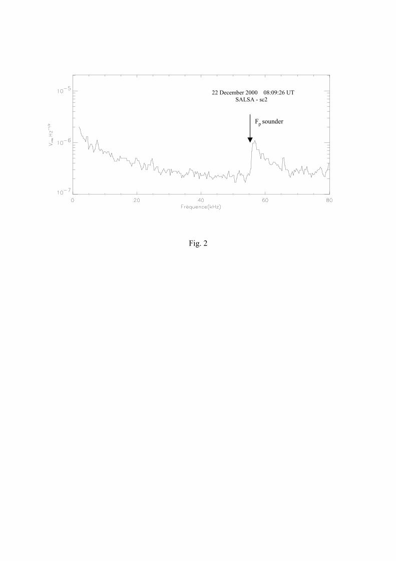
Fig. 2

22 December 2000 08:09:26 UTSALSA - sc2

Fp sounder

Fig. 3

SC3 12:14UTSC3 12:16 UTSC4 12:14 UT

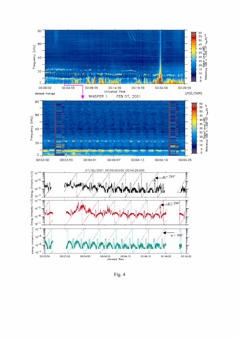
Fig. 4

ϕ = 295°

ϕ = 298°

ϕ = 306°

Fig.5

Fig. 6

SALSA

RUMBA

03:40 04:05 04:30 UT

Fp

(kHz)

-Z

+X Oct 06 2000 04:

04:06 04:18 04:30 UT

tS

tR

Fig. 7

Fig. 8

t3 t2 t1 t4SC1

SC3SC2

SC4

Fig. 9

(kHz)

50

20

Fp

50

20

50

20

50

20

60

40

20

0

RUMBA

SAMBA

SALSA

TANGO

SC1

SC3SC2

SC4

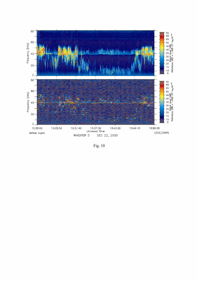
Fig. 10

Fig. 11

Fig. 12

Fig. 13

0,00,51,01,52,02,53,03,54,04,55,0

12:35:00 12:36:00 12:37:00 12:38:00 12:39:00 12:40:00

Time [UT]

Den

sity

[cm

-3]

RUMBA/SC1SALSA/SC2SAMBA/SC3TANGO/SC4

2

10

20

30

40

Freq

uenc

y [k

Hz]

SALSA/SC2

WHISPER/CLUSTER 12 Dec. 2000

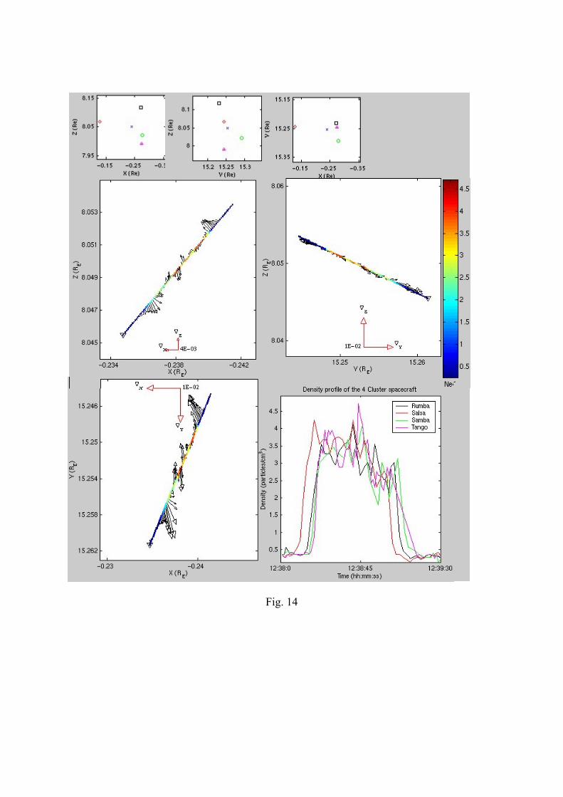
Fig. 14