early detection of first-time slope failures using...

warwick.ac.uk/lib-publications

Original citation: Smith, A., Dixon, Neil and Fowmes, Gary J.. (2017) Early detection of first-time slope failures using acoustic emission measurements : large-scale physical modelling. Geotechnique, 67 (2). pp. 138-152. Permanent WRAP URL: http://wrap.warwick.ac.uk/85722 Copyright and reuse: The Warwick Research Archive Portal (WRAP) makes this work of researchers of the University of Warwick available open access under the following conditions. This article is made available under the Creative Commons Attribution 4.0 International license (CC BY 4.0) and may be reused according to the conditions of the license. For more details see: http://creativecommons.org/licenses/by/4.0/ A note on versions: The version presented in WRAP is the published version, or, version of record, and may be cited as it appears here. For more information, please contact the WRAP Team at: [email protected]

http://go.warwick.ac.uk/lib-publications

http://go.warwick.ac.uk/lib-publications

http://wrap.warwick.ac.uk/85722

http://creativecommons.org/licenses/by/4.0/

mailto:[email protected]

Early detection of first-time slope failures using acoustic emissionmeasurements: large-scale physical modelling

A. SMITH�, N. DIXON� and G. J. FOWMES�

Early warning systems for slope instability need to alert users of accelerating slope deformationbehaviour to enable safety-critical decisions to be made. This study shows that acoustic emission (AE)monitoring of active waveguides (i.e. a steel tube with a granular backfill surround installed through aslope) can both detect shear surface development and quantify increasing rates of movement duringslope failure, thereby providing an early detection of slope instability. A large-scale physical model wasdesigned and built to simulate slope failures on elements of soil, through which full-scale activewaveguides were installed. A shear surface develops in each test and the sliding mass accelerates duringfailure, reaching velocities greater than 300 mm/h and shear deformations of 50 mm. Continuousmeasurements were obtained to examine the behaviour of activewaveguides subjected to first-time slopefailure dynamics (i.e. development of new shear surfaces and accelerating deformation behaviour).Comparisons with continuous subsurface deformation measurements show that AE detection beganduring shear surface formation, and AE rates increased proportionally with displacement ratesas failure occurred. Empirical AE rate–slope velocity relationships are presented for three granularbackfill types, which demonstrate that generic AE rate–slope velocity relationships can be obtained forgroups of backfill types; these relationships allow displacement rates to be quantified from measuredAE rates to provide early detection of slope instability.

KEYWORDS: deformation; failure; field instrumentation; landslides; monitoring; slopes

INTRODUCTIONShear surfaces can develop in slopes formed of strain-softeningmaterials (e.g. overconsolidated clay) after very small defor-mations (millimetres) (Skempton, 1985; Bromhead, 2004).Shear zones develop when the shear stress exceeds the peakshear strength locally within the slope, causing reductions instrength to occur. These shear zones propagate through theslope, developing a continuous shear surface, leading to slopefailure (Skempton, 1964; Skempton & Petley, 1967; Chandler,1984; Leroueil, 2001). These first-time failures can have highpost-failure velocities and experience large displacements,leading to potentially catastrophic consequences. During thisfailure process, the rate of movement increases by orders ofmagnitude; from the gradual development of a shear surfaceproducing low velocities, to the high velocities that are reachedafter the shear surface forms, shear strength reduces and failureoccurs. Early warning of this process (i.e. shear surface devel-opment and accelerating deformation behaviour) is critical toenable evacuation of vulnerable people and timely repair andmaintenance of critical infrastructure.

The Selborne cutting stability experiment (Cooper et al.,1998) provides a detailed example of a first-time failure.The progressive failure process began at the toe of the slopeshortly after the cutting was formed, and the shear surfaceretrogressed up-slope leading to failure 596 days later.Pore-water pressure recharge (i.e. leading to increased pore-water pressures within the body of the slope) was initiated on

day 400, and at this time shear surface displacements of afew millimetres were measured near the toe of the slope.Between days 584 and 589, the slope had accelerated andwasmoving at an average rate of 0·6 mm/h. This acceleratingbehaviour continued and the rate of movement increasedfrom 4 mm/h to 58 mm/h on day 596 when the instrumentsbecame damaged and no longer readable, due to tens ofmillimetres of accumulated displacement. The slope con-tinued to accelerate until failure occurred.Researchers over a period of several decades have

developed slope monitoring strategies using measurementand quantification of acoustic emission (AE) generated bydeforming soil (e.g. Koerner et al., 1981; Chichibu et al.,1989; Nakajima et al., 1991; Rouse et al., 1991; Fujiwaraet al., 1999; Dixon et al., 2003, 2015a; Smith et al., 2014a).These approaches typically employ waveguides (e.g. steeltubes) to provide low attenuation propagation paths for AEto be transmitted from the depth of the shear surface toground level. Monitoring strategies have also been developedusing ‘noisy’ backfill material placed around the waveguidethat generate quantifiable AE (i.e. AE is measured fromthe backfill material and not from the host slope material)when deformed by the host slope, and these are termed‘active’ waveguides (e.g. Dixon et al., 2003; Smith & Dixon,2015). AE monitoring of active waveguides offers manybenefits over traditional deformation monitoring techniques,which include: the subsurface materials are low in cost andeasily sourced, which enables them to be used widely both indeveloped and developing countries; continuous and real-time measurements can be provided at relatively low costbecause of low-cost electronics (in comparison to in-placeinclinometer systems); and they continue to operate at largerdisplacements (.400 mm of shear surface displacement)than other conventional techniques (Dixon et al., 2015b).Active waveguides are installed in boreholes, or retrofitted

inside existing inclinometer or standpipe casings, that inter-sect existing or potential shear surfaces beneath the slope,

� School of Civil and Building Engineering, LoughboroughUniversity, Leicestershire, UK.

Manuscript received 7 September 2015; revised manuscript accepted8 July 2016. Published online ahead of print 19 September 2016.Discussion on this paper closes on 1 July 2017, for furtherinformation see p. ii.Published with permission by the ICE under the CC-BY license.(http://creativecommons.org/licenses/by/4.0/)

Smith, A. et al. (2017). Géotechnique 67, No. 2, 138–152 [http://dx.doi.org/10.1680/jgeot.15.P.200]

138

Downloaded by [] on [06/02/17]. Published with permission by the ICE under the CC-BY license

http://creativecommons.org/licenses/by/4.0/

and they comprise the composite system of a steel tube witha granular backfill surround (Fig. 1). As the host slopedeforms, the active waveguide deforms, and this causesparticle–particle and particle–waveguide interactions totake place, which generate the AE. AE generation mechan-isms include friction (rolling and sliding friction) and colli-sions (e.g. particle contact network rearrangement andrelease of contact stress as interlocking is overcome andregained) (Lord & Koerner, 1974; Koerner et al., 1981;Michlmayr et al., 2013; Michlmayr & Or, 2014).Trials in reactivated slopes have established that there is

a direct relationship between slope displacement rates andactive waveguide-generated AE rates (Smith et al., 2014a,2014b; Smith, 2015; Dixon et al., 2015a, 2015b). To date,these trials have been in slopes with an already formed anddefined shear surface at (or near) residual shear strength thatmove in surges of modest speed (,0·3 mm/h) and travel(,6 mm) in response to rainfall-induced pore-water pressureelevations. Generated AE rates are proportional to applieddisplacement rates because an increasing rate of deformation(i.e. in response to increasing slope velocity) generates anincreasing number of particle–particle and particle–wave-guide interactions per unit time. Each particle interactiongenerates transient AE events, which combine and propagatealong the waveguide where they are monitored at the groundsurface.This study was conducted to investigate the potential

of using active waveguide-generated AE measurements toprovide early detection of first-time slope failure. The objec-tives of the study were: to investigate the use of AE measure-ments to detect accelerating deformation behaviour in amodel that applies a realistic shear mechanism to full-scaleactive waveguides; to establish relationships between applieddisplacement rates and measured AE rates for applied dis-placement rates greater than those measured in field trials todate (i.e. .0·3 mm/h); to investigate the use of the techniqueto detect the formation of new shear surfaces; and toinvestigate the influence of different backfill materials onthe AE generated by active waveguides.A large-scale physical model was designed and built to

simulate slope failures on elements of soil, through whichfull-scale active waveguides were installed. A shear surfacedevelops in each test and the sliding mass accelerates duringfailure, reaching velocities greater than 300 mm/h and sheardeformations of 50 mm. Continuous measurements were

obtained to examine the behaviour of active waveguidessubjected to first-time slope failure dynamics (i.e. shearsurface formation and accelerating deformation behaviour).This experiment has allowed the examination of full-scaleactive waveguides, which ensures the results from the studyare applicable to active waveguide field installations in realslopes.

APPARATUS DEVELOPMENTANDEXPERIMENTAL PROCEDUREDesign considerationsConstructing a full-scale slope and inducing it to fail

through pore-water pressure recharge (i.e. comparable to theSelborne experiment in Cooper et al. (1998)) or removal ofsupport and stress relief through excavations of the toe (i.e.comparable to the Arseley experiment in Dixon et al. (2003))can be used to examine the behaviour of active waveguidessubjected to slope failure. However, it was preferable todevelop a large-scale physical model as this would allowrepeat testing, more variables could be controlled, and agreater understanding of the materials, the stress regime andthe shear surface could be achieved. An important consider-ation in the design of the physical model was the stiffnessmoduli of the steel waveguide, which when present througha full-scale slope moving en masse are negligible; however,when installed through a physical model could cause signific-ant resistance to deformation. The design of the apparatusneeded to include sufficient strength and mass to represent ahost landslide mass, and the method of load applicationneeded to be sufficient to replicate typical accelerations andmagnitudes of waveguide system deformation.

Slope failure apparatusThe apparatus was designed to allow full-scale active wave-

guides to be tested under conditions (e.g. shear mechanism,stresses, displacements and displacement rates) analogous tothose they would experience in a slope undergoing first-timefailure in the field. The apparatus was a bespoke large shearbox (Figs 2 and 3), which comprised two concrete blocks,each with external dimensions 1·0� 0·7� 0·7 m. The bottombox was fixed to a reinforced concrete floor to preventmovement and the top box was placed on top of the bottombox. Each box had an open column (0·3� 0·3 m), which

Signal processing andAE rate quantification bymeasurement node (b)

Quantification of slope velocityusing calibration AE rate–

velocity relationship

Classification of slope velocityusing the standard Cruden &

Varnes (1996) scale (c)

Send warning to decisionmaker to allow action to

be taken

AE generated by activewaveguide in response to

slope movement (a)

Classification

Extremely rapid

Very rapid

Rapid

Moderate

Slow

Very slow

Extremely slow

Velocity

5 m/s

3 m/min

1·8 m/h

13 m/month

1·6 m/year

15 mm/year

Amplitude: V

Time

Threshold level: V

Ring-down counts (RDC)

(a)

(b) (c)

Surface cover

Stable stratumShear surface

Ground surface

Granular backfill

Steel waveguide

Transducer

AE measurement node

Deforming slide mass

Grout plug

Fig. 1. Operation schematic diagram of the AE active waveguide early warning system. (a) and (b) are modified after Smith et al. (2014a)

EARLY DETECTION OF SLOPE FAILURES USING ACOUSTIC EMISSION 139


was filled with soil to represent an element of the slope.A full-scale active waveguide was installed through this soilcolumn. Although there are boundary effects at the soilcolumn–box wall interface, the influence of these is assumedto be negligible at the active waveguide located within the soilcolumn. The modelled system is therefore representative ofa full-scale field active waveguide system when installedthrough a slope and intersecting an existing or potentialshear surface(s).

The open column was offset at the shear box interface toallow for travel of the active waveguide through the soilcolumn; a greater volume of soil is to the rear of the activewaveguide in the top box relative to the volume of soil in frontof it, and the opposite is the case in the bottom box. Smoothhigh-density polyethylene (HDPE) geomembrane (2 mmthick) was fixed to the bottom of the top box and to thetop of the bottom box to form a shear surface with low inter-face friction and allow for repeatable interface behaviour.

A pulley system (Figs 2 and 3) connects the top box to ahydraulically controlled loading ram, which was used to

apply load and displacement to the shear box. The loadingram moves upwards, which pulls the wire rope around thesheave block, and moves the top box horizontally to induceshearing in the soil column. The wire rope was fixed in thefront of the top box using an eye anchor and high-strengthresin. The sheave block was fixed to a reaction frame at theappropriate elevation, which was fixed to the reinforcedconcrete floor. The entrance of the wire rope into the sheaveblock is 2 cm above the elevation of the resin anchor, togenerate a small vertical component of force at the front ofthe top box during the experiments to reduce the frictionalforce at the shear box interface further.

Soil slope elementThe soil slope element was processed Mercia Mudstone,

comprising very silty clay of low plasticity (properties inTable 1). The clay was compacted with as-placed moisturecontents in the range 16·6–19·9% (Table 2; measured fromat least six samples during each test set-up). This was

GeomembraneinterfaceClay

columnoffset

ClayConcrete

Waveguide

Strong floor fixings

Granular backfill

Sheave block

Wire rope

Anchor

Reaction frame

(a)

(b)

(c)

B

Clay Waveguide

Clay

Concrete

Granular backfill

SAA

Concrete

Grouted accesscasing

Geomem-brane

interface

Granular backfill

Waveguide

Groutedaccesscasing

SAA

1000 mm

A'

A

Movement

B'

Fig. 2. Annotated illustration of the first-time slope failure experiment at the start of a test (t=0). The top block is pulled horizontally to the rightof the image by the wire rope during the test. The anchor, wire rope and pulley system are fastened centrally in the horizontal plane and are onlyshown on cross-section B–B′ for illustrative purposes. The figure is to scale and has a dimension line for reference: (a) plan view; (b) cross-sectionA–A′; (c) cross-section B–B′

SMITH, DIXON AND FOWMES140


done to ensure the clay would fail plastically when sheared(i.e. a moisture content marginally wet of both the optimummoisture content and the plastic limit).The clay was compacted in layers using vibration from a

breaker-hammer with a square foot (16� 16 cm), whichapplied cycles of normal force to each layer. The clay wascompacted in five layers in each box in test 1, each using1 min of vibration. It became apparent during excavationof this test that this method of compaction left numerousvoids, which became filled with bentonite-grout when theShapeAccelArray (SAA) was installed (described in the nextsection entitled ‘Instrumentation’). Therefore, the clay wascompacted in ten layers in each box in test 2, each using2·5 min of vibration; this method resulted in successful com-paction with no noticeable voids during excavation. Thecompaction effort required was less due to the material beingless stiff in tests 3 and 4 (higher moisture content); 2 min ofvibration were required for each layer in these tests. Test 5used the same compaction effort as test 2.

InstrumentationTwo 60 mm dia. holes were hand augered through the soil

column (Figs 2 and 3). An active waveguide was installedin one of these holes, which comprised a 22 mm dia., 1·8 mlong steel tube with 2 mm wall thickness (waveguides withthe same geometry and properties are used in field

installations). The annulus around the waveguide was back-filled with granular soil and compacted in 0·2 m high lifts(the same materials and installation procedure are used infield installations). The waveguide protruded 0·4 m abovethe top box where the AE measurement system was coupled.A SAA with 0·2 m gauge lengths was installed in thesecond hole. The SAA comprises a string of micro-electro-mechanical systems (MEMS) sensors, which measure three-dimensional displacements continuously, and the SAA hasan accuracy of +/� 1·5 mm over a length of 30 m (Abdounet al., 2013). The bottom SAAMEMS sensor was positionedat a height of 0·1 m above the base of the soil column. TheSAA was installed inside unplasticised polyvinyl chloride(UPVC) access casing and the annulus around the casing wasbackfilled with bentonite-grout (standard installation pro-cedure). Relative proportions of the bentonite-grout mix were1, 0·17 and 0·07 for water, cement and bentonite, respectively.The bentonite-grout was left to harden around the SAA for4 days prior to the start of each test. The SAA recordeddeformation at 30-s intervals. A linear variable differentialtransducer (LVDT) (with accuracy greater than +/� 0·5%)was installed at the rear of the top box to measure horizontalmovement of the block, and the load applied to the ramwas measured using a load cell (with accuracy greater than+/� 0·2%) throughout the experiments.

AE measurement systemA field-viable AE measurement system was used in this

study. This system was used to ensure the results obtained arerelevant to field monitoring applications. The system isdescribed as ‘field-viable’ because it includes functionalityto remove low-frequency background noise (e.g. generatedby construction activity and traffic) and it has low powerrequirements, which makes continuous monitoring for longdurations in the field environment possible. A piezoelectrictransducer was employed to convert the mechanical AE to anelectrical signal. The transducer was a R3alpha (PhysicalAcoustics Corporation) with a 30 kHz resonant frequencyand this was selected to provide sensitivityover the monitoredfrequency range of 20–30 kHz. The transducer is coupled tothe outer wall of the waveguide with a small layer of siliconegel, and held in position using the compressive contactprovided by an elastic band and cable tie. A band pass filterattenuated signals outside the 20–30 kHz range to eliminatelow-frequency background noise (,20 kHz) and to keep themonitored range consistent with that used in field trials(Smith et al., 2014a, 2014b; Smith, 2015; Dixon et al., 2015a,2015b). Amplification of 70 dB was used to improve thesignal-to-noise ratio. Such field instrumentation shouldemploy relatively simple processing to minimise power andstorage capacity requirements. Therefore, ring-down counts(RDCs) per unit time were recorded and these are the units ofmeasured AE rates. AE rates (RDC rates) are the number oftimes the AE signal amplitude crosses a programmablethreshold level within a predefined time period, and thesewere recorded using a comparator. A voltage threshold levelof 0·25 V was used with a monitoring interval of 5 s; theseRDC per 5 s measurements were converted to moreconventional equivalent RDC per hour values.

ConcreteAE

measurementsystem

Transducer

Active waveguide

SAAWire rope

Sheaveblock

Reactionframe

LVDT Geomembraneinterface

Clay

Fig. 3. Annotated photograph of the first-time failure experiment atthe start of a test (t=0)

Table 1. Clay properties

Name Plasticlimit: %

Liquidlimit: %

Plasticityindex: %

Particle density:Mg/m3

Optimum moisturecontent: %

Maximum drydensity: Mg/m3

Clay 14·8 30·0 15·2 2·54 15·5 1·86



Active waveguide backfillsThree granular waveguide backfill materials were used to

investigate the influence of their properties on the AE ratesgenerated from the active waveguide system. The backfillmaterials were selected because they are typical aggregatesand non-specialised materials, and using materials that areeasy to procure facilitates their widespread use. The backfillstested also provided a range of particle sizes to investigate.Three tests were performed, using the same backfill materialin order to evaluate repeatability. Subsequently, two furtherexperiments were performed with other materials. Thematerials were limestone gravel (LSG), Leighton Buzzardsand (LBS) and granite gravel (GG). Photographs of thegranular soils and their particle size distributions are shownin Fig. 4.

Table 2 details which backfills were installed in which testand Table 3 compares their particle size, particle shape andpacking properties. Particle shape parameters, namely

roundness (i.e. angularity), sphericity (i.e. ellipticity orplatiness) and regularity, were determined using two-dimensional images of the particles. Roundness is quantifiedas the average radius of curvature of particle surface featuresrelative to the radius of the maximum sphere that can beinscribed in the particle. Sphericity is quantified as the radiusratio between the largest inscribed and the smallest circum-scribing sphere. Regularity is the mean of roundness andsphericity (Krumbein & Sloss, 1963; Cho et al., 2006;Cavarretta et al., 2010; Zheng & Hryciw, 2015).

Test procedureAll tests were displacement rate controlled, and

displacement–time functions (Table 4) were designed torepresent the deformation behaviour that slopes experienceas they lose strength and accelerate during progressive failure.The slowest rate of movement was the lowest allowable by theloading machine. The duration of the first two stages of theexperiment was progressively increased between test 1 andtest 3 to apply the lowest rates of deformation for greatermagnitudes of deformation. The same function was appliedin tests 3 to 5.The authors designed the experiment to ensure the sliding

mass travelled 50 mm in each test, which required a set-upprotocol to minimise extension of the wire rope during thetests. Before each test, a constant movement rate of0·1 mm/min was applied. Movement was ceased at thepoint at which the LVDT detected movement. After this

Table 2. Test details

Testnumber

Backfill Clay moisturecontent: %

1 Limestone gravel (LSG) 18·62 Limestone gravel (LSG) 17·43 Limestone gravel (LSG) 19·94 Leighton Buzzard sand (LBS) 18·85 Granite gravel (GG) 16·6

0

20

40

60

80

100

0·1 1 10

Fine

r by

mas

s: %

Sieve aperture size: mm(a)

Limestone gravelLeighton Buzzard sandGranite gravel

(b)

(c)

(d)

Fig. 4. (a) Particle size distributions of the granular backfill materials, and photographs of the backfill materials: (b) LSG; (c) LBS; (d) GG

Table 3. Particle size, particle shape and packing properties of the granular backfills

Description Particle size Particle shape Packing

Size range:mm

Coefficientof uniformity

Roundness Sphericity Regularity Particledensity: Mg/m3

Dry density:Mg/m3

Voidratio

Limestone gravel (LSG) 3·0–8·0 1·51 0·3–0·5 0·5–0·8 0·4–0·6 2·64 1·53 0·730Leighton Buzzard sand (LBS) 0·3–1·8 1·93 0·2–0·5 0·4–0·8 0·3–0·6 2·67 1·70 0·567Granite gravel (GG) 5·0–12·0 1·41 0·1–0·3 0·3–0·8 0·2–0·6 2·68 1·58 0·699



initial box movement, the test was in the start position andthe displacement–time function (Table 4) was then applied tothe top box. The LVDT and SAA measured the actualmovement of the top box and the soil column, respectively.The soil column was excavated at the end of each test and theinstruments were removed, prior to setting up the subsequenttest.

RESULTS AND ANALYSISDeformation and load behaviourFigure 5 shows displacement plotted against time

measurements recorded during test 3 by the loading ram,the LVDT, and the SAA MEMS sensor located above theshear surface at a height of 0·9 m (resultant horizontaldeformation); comparable behaviour was measured in eachtest. All SAA time series measurements presented are takenfrom this MEMS sensor, and they are the resultant of thehorizontal deformation. Ram deformation of ,3 mm wastaken up by extension in the wire rope throughout the test,which is evident from the difference between the ram positionand LVDT displacement. A difference of ,1 mm betweenthe LVDT measured block movement and the SAA meas-ured deformation developed during stages 1 and 2, prior toshear surface formation in the clay.Figure 6 shows the height plotted against resultant

horizontal SAA deformation measurements at the end ofeach stage during test 3 (comparable behaviour was measuredin each test). Height is relative to the base of the bottom box.The interface between the two blocks is at a height of 0·7 m,which also corresponds to the location of a MEMS sensor.The apparent shear zone is 0·4 m thick, 0·2 m above andbelow the interface; however, this is because the adjacentMEMS sensors are 0·2 m away. The real shear zone wassignificantly thinner (,2 cm) at a height of 0·7 m; this wasconfirmed by visual inspection during forensic dismantlingof each test.Shear surface formation began in stage 2; this is clear from

the measurements in Fig. 6, which show the SAA rotatingabout its base only during stage 1 (i.e. no relative shearmovement between MEMS sensors is identifiable). The loadplotted against deformation measurements shown in Fig. 7support this as elastic deformation occurs until stage 2 ineach test, at which point a transition to plastic deformationoccurs (i.e. the shear surface forms). This transition is smoothwith no drop in load in tests 1, 2 and 5, whereas in tests 3 and4 a drop in load is identifiable.The differences in load–deformation measurements were

principally governed by the composition of the clay column,for example: tests 1 to 3 used the same active waveguide

backfill but experienced noticeably different behaviour. Theclay installed in tests 3 and 4 had comparable stiffness(moisture content and compaction effort) and experiencedcomparable behaviour. This was also the case for tests 2 and 5.

Table 4. Displacement rate-controlled function applied in tests 3, 4 and 5. Note that stages 1 and 2 were applied for shorter durations intests 1 and 2

Stage Applied displacement rate towire rope Duration: min Cumulative time: min Cumulative displacement: mm

mm/min mm/h

0 01* 0·06 3·6 50 50 32† 0·12 7·2 25 75 63 0·25 15 10 87 94 0·5 30 8 95 135 1 60 5 100 186 2 120 4 104 267 4 240 3 107 388 6 360 3 110 56

*Stage 1 lasted for 15 min in test 1 and 35 min in test 2.†Stage 2 lasted for 10 min in test 1 and 20 min in test 2.

0

10

20

30

40

50

60

0 20 40 60 80 100

Dis

plac

emen

t: m

m

Time: min

Ram position (mm)LVDT displacement (mm)Resultant horizontal SAA displacement (mm)at height = 0·9 m

Fig. 5. Ram position, LVDT displacement and resultant horizontalSAA displacement plotted against time (test 3)

0

0·2

0·4

0·6

0·8

1·0

1·2

1·4

0 10 20 30 40 50

Hei

ght:

m

Displacement: mm

Shear box interface

t = 0

t = 5

0 (s

tage

1)

t = 7

5 (s

tage

2)

t = 8

7 (s

tage

3)

t = 9

5 (s

tage

4)

t = 1

00 (s

tage

5)

t = 1

04 (s

tage

6)

t = 1

07 (s

tage

7)

t = 1

10 (s

tage

8)

Fig. 6. Height above the base of the shear box plotted against SAAmeasured resultant horizontal deformation from test 3 for the end ofeach stage at time t (min)



Test 1 experienced different behaviour: the voids in the clay intest 1 became filled with bentonite-grout that infiltrated whenthe SAA was installed, increasing the strength of the claycolumn.The SAA deformation progressively increased below the

shear surface as the SAAwas pulled horizontally through thebentonite-grout and clay in the bottom box, resulting inbehaviour analogous to a laterally loaded flexible (highslenderness ratio) pile. This mechanism is likely to havebegun earlier, in response to smaller magnitudes of move-ment, in the active waveguide due to its significantly greaterstiffness.

AE and deformation behaviourTests 1 to 3 (repeatability). Figure 8 presents time seriesmeasurements from test 3. The cumulative RDC measure-ments are proportional to the SAA measured displacement,and the AE rate measurements are proportional to the SAAmeasured velocity. Velocity smoothing was done using 2-minmoving average values, by calculating the average of the

2

4

6

8

10

0 5 10 15 20 25 30 35 40 45 50

Load

: kN

Displacement: mm

Test 1Test 2Test 3Test 4Test 5

Transition from elasticto plastic load–displacement behaviour(shear surface develops)

1

2

3

4

5

Fig. 7. Load plotted against displacement data for each test. Notethat displacement is taken from the SAA MEMS sensor immediatelyabove the shear surface (at a height of 0·9 m)

0

1

2

3

4

5

6

7

0

10

20

30

40

50

0 20 40 60 80 100

Cum

ulat

ive

AE

: RD

C ×

100

0

Dis

plac

emen

t: m

m

Time: min

Resultant horizontal SAAdisplacement (mm)at height = 0·9 mCumulative AE (RDC)

(a)

AE detection begins at1·9 mm of sheardisplacement

0

5

10

15

20

–50

0

50

100

150

200

250

300

350

400

0 20 40 60 80 100

AE

rate

: RD

C/h

× 1

0 00

0

Vel

ocity

: mm

/h

Time: min

SAA measured velocity (mm/h)SAA measured velocity(smoothed) (mm/h)AE rate (RDC/h)

(b)

She

ar s

urfa

ce fo

rms

Fig. 8. Time series of measurements from test 3: (a) displacement and cumulative RDC plotted against time; (b) SAAvelocity and AE rate plottedagainst time. AE rates presented are significantly greater than the cumulative RDC because they have been converted to equivalent RDC/h values



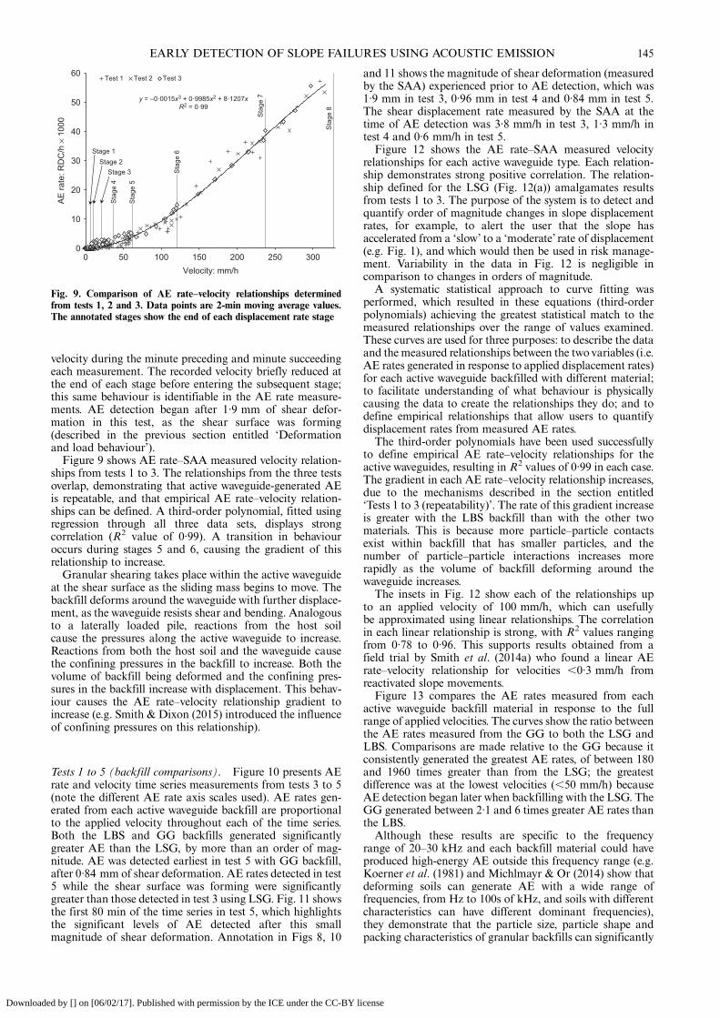
velocity during the minute preceding and minute succeedingeach measurement. The recorded velocity briefly reduced atthe end of each stage before entering the subsequent stage;this same behaviour is identifiable in the AE rate measure-ments. AE detection began after 1·9 mm of shear defor-mation in this test, as the shear surface was forming(described in the previous section entitled ‘Deformationand load behaviour’).Figure 9 shows AE rate–SAA measured velocity relation-

ships from tests 1 to 3. The relationships from the three testsoverlap, demonstrating that active waveguide-generated AEis repeatable, and that empirical AE rate–velocity relation-ships can be defined. A third-order polynomial, fitted usingregression through all three data sets, displays strongcorrelation (R2 value of 0·99). A transition in behaviouroccurs during stages 5 and 6, causing the gradient of thisrelationship to increase.Granular shearing takes place within the active waveguide

at the shear surface as the sliding mass begins to move. Thebackfill deforms around the waveguide with further displace-ment, as the waveguide resists shear and bending. Analogousto a laterally loaded pile, reactions from the host soilcause the pressures along the active waveguide to increase.Reactions from both the host soil and the waveguide causethe confining pressures in the backfill to increase. Both thevolume of backfill being deformed and the confining pres-sures in the backfill increase with displacement. This behav-iour causes the AE rate–velocity relationship gradient toincrease (e.g. Smith & Dixon (2015) introduced the influenceof confining pressures on this relationship).

Tests 1 to 5 (backfill comparisons). Figure 10 presents AErate and velocity time series measurements from tests 3 to 5(note the different AE rate axis scales used). AE rates gen-erated from each active waveguide backfill are proportionalto the applied velocity throughout each of the time series.Both the LBS and GG backfills generated significantlygreater AE than the LSG, by more than an order of mag-nitude. AE was detected earliest in test 5 with GG backfill,after 0·84 mm of shear deformation. AE rates detected in test5 while the shear surface was forming were significantlygreater than those detected in test 3 using LSG. Fig. 11 showsthe first 80 min of the time series in test 5, which highlightsthe significant levels of AE detected after this smallmagnitude of shear deformation. Annotation in Figs 8, 10

and 11 shows the magnitude of shear deformation (measuredby the SAA) experienced prior to AE detection, which was1·9 mm in test 3, 0·96 mm in test 4 and 0·84 mm in test 5.The shear displacement rate measured by the SAA at thetime of AE detection was 3·8 mm/h in test 3, 1·3 mm/h intest 4 and 0·6 mm/h in test 5.Figure 12 shows the AE rate–SAA measured velocity

relationships for each active waveguide type. Each relation-ship demonstrates strong positive correlation. The relation-ship defined for the LSG (Fig. 12(a)) amalgamates resultsfrom tests 1 to 3. The purpose of the system is to detect andquantify order of magnitude changes in slope displacementrates, for example, to alert the user that the slope hasaccelerated from a ‘slow’ to a ‘moderate’ rate of displacement(e.g. Fig. 1), and which would then be used in risk manage-ment. Variability in the data in Fig. 12 is negligible incomparison to changes in orders of magnitude.A systematic statistical approach to curve fitting was

performed, which resulted in these equations (third-orderpolynomials) achieving the greatest statistical match to themeasured relationships over the range of values examined.These curves are used for three purposes: to describe the dataand the measured relationships between the twovariables (i.e.AE rates generated in response to applied displacement rates)for each active waveguide backfilled with different material;to facilitate understanding of what behaviour is physicallycausing the data to create the relationships they do; and todefine empirical relationships that allow users to quantifydisplacement rates from measured AE rates.The third-order polynomials have been used successfully

to define empirical AE rate–velocity relationships for theactive waveguides, resulting in R2 values of 0·99 in each case.The gradient in each AE rate–velocity relationship increases,due to the mechanisms described in the section entitled‘Tests 1 to 3 (repeatability)’. The rate of this gradient increaseis greater with the LBS backfill than with the other twomaterials. This is because more particle–particle contactsexist within backfill that has smaller particles, and thenumber of particle–particle interactions increases morerapidly as the volume of backfill deforming around thewaveguide increases.The insets in Fig. 12 show each of the relationships up

to an applied velocity of 100 mm/h, which can usefullybe approximated using linear relationships. The correlationin each linear relationship is strong, with R2 values rangingfrom 0·78 to 0·96. This supports results obtained from afield trial by Smith et al. (2014a) who found a linear AErate–velocity relationship for velocities ,0·3 mm/h fromreactivated slope movements.Figure 13 compares the AE rates measured from each

active waveguide backfill material in response to the fullrange of applied velocities. The curves show the ratio betweenthe AE rates measured from the GG to both the LSG andLBS. Comparisons are made relative to the GG because itconsistently generated the greatest AE rates, of between 180and 1960 times greater than from the LSG; the greatestdifference was at the lowest velocities (,50 mm/h) becauseAE detection began later when backfilling with the LSG. TheGG generated between 2·1 and 6 times greater AE rates thanthe LBS.Although these results are specific to the frequency

range of 20–30 kHz and each backfill material could haveproduced high-energy AE outside this frequency range (e.g.Koerner et al. (1981) and Michlmayr & Or (2014) show thatdeforming soils can generate AE with a wide range offrequencies, from Hz to 100s of kHz, and soils with differentcharacteristics can have different dominant frequencies),they demonstrate that the particle size, particle shape andpacking characteristics of granular backfills can significantly

y = –0·0015x3 + 0·9985x2 + 8·1207xR2 = 0·99

0

10

20

30

40

50

60

0 50 100 150 200 250 300

AE

rate

: RD

C/h

× 1

000

Velocity: mm/h

Test 1 Test 2 Test 3

Stage 1Stage 2

Stage 3

Sta

ge 4

Sta

ge 5

Sta

ge 6

Sta

ge 7

Sta

ge 8

Fig. 9. Comparison of AE rate–velocity relationships determinedfrom tests 1, 2 and 3. Data points are 2-min moving average values.The annotated stages show the end of each displacement rate stage



influence the AE they produce. The GG had the largestparticles with the greatest angularity (Table 3). The LBS hadthe greatest coefficient of uniformity and lowest void ratio(densest packing). The LSG had the highest void ratio and itsparticles had the lowest angularity.

DISCUSSIONA series of experiments have been performed to

subject full-scale active waveguides to the conditionsthey would experience when installed through a slopeundergoing first-time failure. The conditions of the failure

process were informed by the Selborne cutting stabilityexperiment (Cooper et al., 1998). A shear surface formsin each test and the sliding mass gradually acceleratesfrom displacement rates ,0·5 mm/h to rates .300 mm/h.Measured AE rates have been shown to increase proportion-ally with the applied rates of shear displacement, in each test,with each backfill. This demonstrates that the AE monitor-ing approach can be used to quantify slope displacementrates from measured AE rates using calibration AE rate–velocity relationships. This information can provide earlydetection of accelerating deformation behaviour that slopesexperience during failure.

0

2

4

6

8

10

12

14

16

18

–50

0

50

100

150

200

250

300

350

400

0 20 40 60 80 100

AE

rate

: RD

C/h

× 1

000

000

Vel

ocity

: mm

/h

Time: min

SAA measured velocity(mm/h)SAA measured velocity(smoothed) (mm/h)AE rate (RDC/h)

She

ar s

urfa

ce fo

rms

AE detection beginsat 0·84 mm of shear

displacement

(c)

0

1

2

3

4

5

6

7

8

9

–50

0

50

100

150

200

250

300

350

400

0 20 40 60 80 100

AE

rate

: RD

C/h

× 1

000

000

Vel

ocity

: mm

/h

Time: min

SAA measured velocity (mm/h)

SAA measured velocity(smoothed) (mm/h)AE rate (RDC/h)

She

ar s

urfa

ce fo

rms

AE detection beginsat 0·96 mm of shear

displacement

(b)

0

5

10

15

20

–50

0

50

100

150

200

250

300

350

400

0 20 40 60 80 100

AE

rate

: RD

C/h

× 1

0 00

0

Vel

ocity

: mm

/h

Time: min

SAA measured velocity (mm/h)SAA measured velocity(smoothed) (mm/h)AE rate (RDC/h)

She

ar s

urfa

ce fo

rms

AE detection beginsat 1·9 mm of sheardisplacement

(a)

Fig. 10. AE rate and velocity plotted against time from tests 3, 4 and 5: (a) LSG; (b) LBS; and (c) GG. Note the different AE rate axis scales used



The majority of the measurements in this study were madeat displacement rates above 0·5 mm/h; however, previousresearch through field trials reported by the authors inSmith et al. (2014a) demonstrates that the AE monitoringtechnique can measure slope displacement rates below0·3 mm/h once a continuous shear surface has formed(example AE rate–velocity measurements from this fieldstudy are shown in Fig. 14). The mechanisms of shear surfaceformation in the tests reported here prevented the examin-ation of ‘extremely slow’ displacement rates. This is becausethe magnitude and rate of displacements are linked; morethan 0·7 mm of deformation was required to overcome theapparatus compliance and begin to form the shear surfacein each test, and it would be impractical to apply ‘extremelyslow’ displacement rates during this test phase because itwould take days, even weeks, for the shear surface to form.Shearing was induced in the active waveguide

when the shear surface began to form, initiating particle–-particle/particle–waveguide interactions, which generatedAE. AE detection began at the onset of shear surface

formation when using waveguides backfilled with the GGand LBS; however, when using waveguides backfilled withthe LSG, AE detection began after the majority of the shearsurface had already formed. This is a significant findingbecause knowledge of when a shear surface is forming withina slope can contribute to improving slope risk management.Empirical AE rate–slope velocity relationships were

derived for three different active waveguide backfill types,which allow slope displacement rates to be quantifiedfrom measured AE rates when using these instrumentsand monitoring in the 20–30 kHz range. These empiricalrelationships allow Class A (Lambe, 1973) a priori predic-tions to be made about how the active waveguide will respond(i.e. the AE rates it will generate) to a range of slopemovement rates as first-time failure develops. This has beendemonstrated by performing multiple tests with the sameactive waveguide backfill (LSG), which confirms that theseAE rate–displacement rate relationships are repeatable.Figure 15 shows how these relationships can be used to

derive AE rate warning trigger levels, based on slope

0

1

2

3

4

5

6

–50

–40

–30

–20

–10

0

10

20

30

40

50

AE ra

te: R

DC

/h ×

100

000

SAA measured velocity (mm/h)

SAA measured velocity (smoothed)(mm/h)AE rate (RDC/h)

0

1

2

3

4

5

6

7

0

1

2

3

4

5

0 20 40 60 80

Cum

ulat

ive

AE

: RD

C ×

10

000

Time: min(a)

(b)

0 20 40 60 80Time: min

Vel

ocity

: mm

/hD

ispl

acem

ent:

mm

Resultant horizontal SAA displacement (mm) at height = 0·9 m

Cumulative AE (RDC)

She

ar s

urfa

ce fo

rms

AE detection beginsat 0·84 mm of shear displacement

Fig. 11. Time series of measurements from the first 80 min of test 5: (a) displacement and cumulative RDC plotted against time; (b) velocity andAE rate plotted against time. AE rates presented are significantly greater than the cumulative RDC because they have been converted to equivalentRDC/h values



0

2

4

6

8

10

0 100 200

(c)

300

AE

rate

: RD

C/h

× 1

000

000

Velocity: mm/h

Stage 1Stage 2

Stage 3

Sta

ge 4 Sta

ge 5 Sta

ge 6

Sta

ge 7

Sta

ge 8

y = –0·0015x3+ 0·9985x2 + 8·1207xR2 = 0·99

0

10

20

30

40

50

60

0 100 200

(a)

300

AE

rate

: RD

C/h

× 1

000

10

20

30

40

50

AE

rate

: RD

C/h

× 1

0000

0

Velocity: mm/h

Stage 1Stage 2

Stage 3

Sta

ge 4

Sta

ge 5

Sta

ge 6

Sta

ge 7

Sta

ge 8

y = 61xR2 = 0·78

02468

10

0 50 100

× 10

00

00 100 200 300

Velocity: mm/h

Stage 1Stage 2

Stage 3

Sta

ge 4

Sta

ge 5

Sta

ge 6

Sta

ge 7

Sta

ge 8

y = 2746xR2 = 0·85

012345

0 50 100

× 10

000

0

0

1

2

0 50 100

× 10

0000

0

y = 0·1526x3 – 5·0868x2 + 2922·7xR2 = 0·99

y = 0·0614x3 + 35·998x2 + 16 162xR2 = 0·99

(b)

y = 17 976xR2 = 0·96

Fig. 12. Comparison of AE rate–velocity relationships determined from experiments on each backfill type: (a) LSG; (b) LBS; (c) GG. The insetsshow the AE rate–velocity relationships up to a velocity of 100 mm/h. Data points are 2-min moving average values. The annotated stages show theend of each stage



displacement rates, which can be used to quantify andcommunicate accelerations in slope movement during failure(i.e. in the process shown in Fig. 1). A generic relationshiphas been produced in Fig. 15 by combining the empiricalrelationships derived from both GG and LBS backfills. Thisdemonstrates that such generic relationships can be definedfor groups of different backfill materials, removing the needfor specialised calibration of each backfill material used, toquantify order of magnitude changes in slope displacementrates from measured AE rates, to provide early warning.The results have revealed that active waveguides experience

behaviour comparable to laterally loaded piles when sub-jected to slope movement. The predominant AE generationmechanism is granular shearing at the shear surface at smallmagnitudes of deformation; however, the volume of backfillbeing deformed and the confining pressures in the backfillincrease with displacement and this behaviour causesthe AE rate–velocity relationship gradient to increase.These results have implications for designing the embedmentdepth for active waveguide installations, because the positionat which the shear surface intersects the active waveguidealong its length will govern how it interacts with the host soil

(e.g. Poulos, 1995), which will also influence the AE rate–slope velocity relationship that it produces. In addition,active waveguides installed in reactivated slopes that experi-ence multiple surge movements will be subjected to cycles ofstress and stress relaxation, and their geometry will changeover time, modifying the AE rate–slope velocity relationshipsthey produce.Practical considerations when selecting backfill materials

include: ease of compaction around the waveguide to ensureno large voids are present; and the AE propagation distance(i.e. depth to the shear surface) as low-amplitude backfill-generated AE will be attenuated before being detected.Relatively single-sized granular soils can be compactedeasily around the waveguide, and this is why they are typicallyused as backfills (Smith et al., 2014a, 2014b; Smith, 2015;Smith & Dixon, 2015; Dixon et al., 2015a, 2015b). Backfillswith large angular particles generate the highest amplitudeAE (e.g. Table 3 and Fig. 13), and these are required forslopes with deep shear surfaces to mitigate the attenuationof AE propagating long distances along the steel tube.Particle size also governs the number of particle–particleinteractions and how rapidly this number of interactions

0

1

2

3

4

5

6

7

0 50 100 150

(a)

(b)

200 250 300

AE

rate

ratio

, GG

/LB

S

Velocity: mm/h

GG/LBS

0

500

1000

1500

2000

0 50 100 150 200 250 300

AE

rate

ratio

, GG

/LS

G

Velocity: mm/h

GG/LSG

Fig. 13. Ratio of AE rates generated by the GG backfill to the other backfills plotted against applied velocity: (a) GG/LBS; (b) GG/LSG



increases as the backfill volume undergoing deformationincreases, which influences the shape of the AE rate–velocityrelationship.

The monitored range of 20–30 kHz was selected to ensurethe results from this study are relevant to field monitoringapplications, which use such a frequency range to minimisebackground noise. However, monitoring a wider bandincluding lower frequencies would allow AE to be detectedearlier; in this study AE below 20 kHz were not detected. Itis anticipated that AE detection would begin at smallerdisplacements when monitoring a wide frequency band, ifwell-graded backfills with low void ratio, and large particleswith high angularity and high surface roughness, were used.This study has demonstrated that these soil properties (e.g.

Table 3) significantly influence AE generation. These back-fills would generate the greatest number of transient AEevents per unit time (i.e. frequency) because they not onlyhave a greater number of particle–particle and particle–waveguide contacts; they also have more particle surfacefeature contacts that generate AE during relative particlemovement.

CONCLUSIONSThis study was conducted to investigate the potential of

using active waveguide-generated AE measurements toprovide an early detection of first-time slope failure. The

0

0·1

0·2

0·3

0·4

0

10

20

30

40

50

60

70

80

0 2 4 6 8 10 12 14 16 18 20 22

Vel

ocity

: mm

/h

AE

rate

: RD

C/h

Time: d(a)

(b)

AE

SAA

y = 98xR2 = 0·8

0

5

10

15

20

25

30

35

0 0·05 0·10 0·15 0·20 0·25 0·30

AE

rate

: RD

C/h

Velocity: mm/h

Fig. 14. AE rate and SAA velocity measurements obtained for a series of reactivated slide events (<0·3 mm/h) from a field trial reported inSmith et al. (2014a). These data show that AE monitoring is able to detect slope displacement rates below those examined in this study.(a) AE rate and SAA measured velocity time series measurements (grey lines) and smoothed curves of moving average values (black lines).(b) AE rate plotted against SAA measured velocity relationship derived from the series of reactivated slide events shown in (a) (modified afterSmith et al., 2014a)



principal findings are summarised in the followingconclusions.

(a) Evidence has been obtained showing that AEmonitoring of active waveguides can both detect shearsurface development and quantify increasing rates ofmovement during slope failure, thereby providing anearly detection of slope instability. The majority of themeasurements in this study to support this conclusionwere made at displacement rates above 0·5 mm/h;however, these findings are supplemented by previousresearch reported by the authors in Smith et al.(2014a), which demonstrates performance of the AEmonitoring technique below slope displacement ratesof 0·3 mm/h.

(b) Empirical AE rate–slope velocity relationships havebeen defined for three different active waveguidebackfill types, which allow slope displacement ratesto be quantified from measured AE rates.

(c) Evidence has been obtained showing that genericAE rate–slope velocity relationships can be developedfor groups of granular backfill materials, removing theneed for specialised calibration of each backfill materialemployed, which can be used to quantify order ofmagnitude changes in slope displacement rates frommeasured AE rates to provide early detection of slopeinstability.

(d ) The choice of backfill can significantly influence theAE rate–slope velocity relationship, both in terms ofmagnitude and distribution with time. Backfill withlarge, angular particles produced AE responses withthe greatest magnitude and began generating detectableAE the earliest. Further research is required to achievea greater understanding of how the properties ofgranular soil influence the AE they produce.

ACKNOWLEDGEMENTSThe support provided by the Engineering and Physical

Sciences Research Council (EP/H007261/1, EP/D035325)and Loughborough University is gratefully acknowledged.The authors also acknowledge the collaboration with PhilipMeldrum, British Geological Survey, in development of theAE measurement system used in this study, and the excellent

technical assistance provided by Mr Lewis Darwin. Datareported in this study can be made available by the authorson request.

REFERENCESAbdoun, T., Bennett, V., Desrosiers, T., Simm, J. & Barendse, M.

(2013). Asset management and safety assessment of Leveesand Earthen Dams through comprehensive real-time fieldmonitoring. Geotech. Geol. Engng 31, No. 3, 833–843.

Bromhead, E. N. (2004). Landslide slip surfaces: their origins,behaviour and geometry. In Landslides: evaluation and stabiliz-ation (eds W. A. Lacerda, M. Ehrlich, S. A. B. Fontoura andA. S. F. Sayão), pp. 3–21. Boca Raton, FL, USA: CRC Press.

Cavarretta, I., Coop, M. & O’Sullivan, C. (2010). The influenceof particle characteristics on the behaviour of coarse grainedsoils. Géotechnique 60, No. 6, 413–423, http://dx.doi.org/10.1680/geot.2010.60.6.413.

Chandler, R. J. (1984). Recent European experience of landslidesin over-consolidated clays and soft rocks. Proceedings of the4th international symposium on landslides, Toronto, Canada,pp. 61–80.

Chichibu, A., Jo, K., Nakamura, M., Goto, T. & Kamata, M.(1989). Acoustic emission characteristics of unstable slopes.J. Acoustic Emission 8, No. 4, 107–112.

Cho, G. C., Dodds, J. & Santamarina, J. C. (2006). Particle shapeeffects on packing density, stiffness, and strength: natural andcrushed sands. J. Geotech. Geoenviron. Engng 132, No. 5,591–602.

Cooper, M. R., Bromhead, E. N., Petley, D. J. & Grants, D. I.(1998). The Selborne cutting stability experiment. Géotechnique48, No. 1, 83–101, http://dx.doi.org/10.1680/geot.1998.48.1.83.

Cruden, D. M. & Varnes, D. J. (1996). Landslide typesand processes. In Landslides: investigation and mitigation(eds A. K. Turner and L. R. Schuster), TRB special report247, Ch. 3. Washington, DC, USA: Transportation ResearchBoard.

Dixon, N., Hill, R. & Kavanagh, J. (2003). Acoustic emissionmonitoring of slope instability: Development of an activewave guide system. Proc. Instn Civ. Engrs – Geotech. Engng156, No. 2, 83–95.

Dixon, N., Spriggs, M. P., Smith, A., Meldrum, P. & Haslam, E.(2015a). Quantification of reactivated landslide behaviourusing acoustic emission monitoring. Landslides 12, No. 3,549–560.

Dixon, N., Smith, A., Spriggs, M. P., Ridley, A., Meldrum, P. &Haslam, E. (2015b). Stability monitoring of a rail slope usingacoustic emission. Proc. Instn Civ. Engrs – Geotech. Engng 168,No. 5, 373–384.

0·1

1

10

100

1000

10 000

100 000

1 000 000

10 000 000

100 000 000

0·00001 0·0001 0·001 0·01 0·1 1 10 100Velocity: mm/h

AE

rate

: RD

C/h

Extremely slow Very slow Slow Moderate

Granite gravel

LeightonBuzzard sand

Very slow threshold

Slow threshold

Moderate threshold

Fig. 15. AE rate–velocity calibration relationships derived for GG and LBS plotted on log scales, with the standard landslide velocity scale(Cruden & Varnes, 1996) superimposed, demonstrating that generic relationships can be obtained for groups of backfills to determine AE ratewarning trigger levels based on slope displacement rates



http://dx.doi.org/10.1680/geot.2010.60.6.413











Fujiwara, T., Ishibashi, A. & Monma, K. (1999). Applicationof acoustic emission method to Shirasu slope monitoring.In Slope stability engineering (eds N. Yagi, T. Yamagami andJ. C. Jiang), pp. 147–150. Rotterdam, the Netherlands: Balkema.

Koerner, R. M., McCabe, W. M. & Lord, A. E. (1981). Acousticemission behaviour and monitoring of soils. InAcoustic emissionin geotechnical practice (eds V. P. Drnevich and R. E. Gray),ASTM STP 750, pp. 93–141. West Conshohocken, PA, USA:ASTM International.

Krumbein, W. C. & Sloss, L. L. (1963). Stratigraphy and sedimen-tation, 2nd edn. San Francisco, CA, USA: Freeman andCompany.

Lambe, T. W. (1973). Predictions in soil engineering. Géotechnique23, No. 2, 151–202, http://dx.doi.org/10.1680/geot.1973.23.2.151.

Leroueil, S. (2001). Natural slopes and cuts: movement and failuremechanisms.Géotechnique 51, No. 3, 197–243, http://dx.doi.org/10.1680/geot.2001.51.3.197.

Lord, A. E. & Koerner, R. M. (1974). Acoustic emission response ofdry soils. J. Testing and Evaluation (ASTM) 2, No. 3, 159–162.

Michlmayr, G. & Or, D. (2014). Mechanisms for acoustic emissionsgeneration during granular shearing. Granular Matter 16, No. 5,627–640.

Michlmayr, G., Cohen, D. & Or, D. (2013). Shear-induced forcefluctuations and acoustic emissions in granular material.J. Geophys. Res.: Solid Earth 118, No. 12, 6086–6098.

Nakajima, I., Negishi, M., Ujihira, M. & Tanabe, T. (1991).Application of the acoustic emission monitoring rod to landslidemeasurement. In Acoustic emission/microseismic activity ingeologic structures and materials: proceedings of the 5th conference(ed. H. R. Hardy), pp. 505–519. Pfaffikon, Switzerland:Trans Tech.

Poulos, H. G. (1995). Design of reinforcing piles to increase slopestability. Can. Geotech. J. 32, No. 5, 808–818.

Rouse, C., Styles, P. & Wilson, S. A. (1991). Microseismic emissionsfrom flowslide-type movements in South Wales. Engng Geol. 31,No. 1, 91–110.

Skempton, A. W. (1964). Long-term stability of clay slopes,Fourth Rankine Lecture. Géotechnique 14, No. 2, 77–101,http://dx.doi.org/10.1680/geot.1964.14.2.77.

Skempton, A. W. (1985). Residual strength of clays in landslides,folded strata and the laboratory. Géotechnique 35, No. 1, 3–18,http://dx.doi.org/10.1680/geot.1985.35.1.3.

Skempton, A.W. & Petley, D. J. (1967). The strength along structuraldiscontinuities in stiff clays. Proceedings of the geotechnicalconference, Oslo, Norway, vol. 2, pp. 29–46.

Smith, A. (2015). Quantification of slope deformation behaviourusing acoustic emission monitoring. PhD thesis, LoughboroughUniversity, Loughborough, UK.

Smith, A. & Dixon, N. (2015). Quantification of landslidevelocity from active waveguide-generated acoustic emission.Can. Geotech. J. 52, No. 4, 413–425.

Smith, A., Dixon, N., Meldrum, P., Haslam, E. & Chambers, J.(2014a). Acoustic emission monitoring of a soil slope: compari-sons with continuous deformation measurements. GéotechniqueLett. 4, No. 4, 255–261.

Smith, A., Dixon, N., Meldrum, P. & Haslam, E. (2014b).Inclinometer casings retrofitted with acoustic real-time moni-toring systems. Ground Engng, October, pp. 24–29.

Zheng, J. & Hryciw, R. D. (2015). Traditional soil particle sphericity,roundness and surface roughness by computational geometry.Géotechnique 65, No. 6, 494–506, http://dx.doi.org/10.1680/geot.14.P.192.



























http://dx.doi.org/10.1680/geot.14.P.192






early detection of first-time slope failures using...

Documents