e.-.,- yv sn-cp-/ j3y - nasa · e.-.,-= yv sn-cp-/ j3y ilvlpact of analysis uncertainty upon...
TRANSCRIPT
e.-.,-
=
YV sn-cp-/ j3y
IlVlPACT OF ANALYSIS UNCERTAINTY UPON
REGIONAL ATMOSPtIERIC MOISTURE FLUX
Muyin Wang and Jan PaegleDepartment of Meteorology
University of Utah, Salt Lake City, Utah 84112
L _
(NASA-CR-197134) ANALYSES AND N95-32933FORECASTS WITH LAgS WINOS Final
Report) 22 Sep. 1993 - 31 Dec. 1994(Utah Univ.) 35 p unclas
G3/47 0063080
December 1994
Revised May 1995
Corresponding author: Jan Paegle, Department of Meteorology, 819WBB, University of Utah,Salt Lake City, UT 84112
https://ntrs.nasa.gov/search.jsp?R=19950026512 2018-08-29T14:06:05+00:00Z

_r L
NASA_CR-l.991--34'
I
\ -
. _ ABSTRACT
/<//J// _ ....
/A r- _/7-c_.-,,_..-"
.3S
Horizontal fluxes of atmospheric water vapor are studied for summer months during 1989
and 1992 over North and South America based on analyses from European Centre for Medium
Range Weather Forecasts, US National Meteorological Center, and United Kingdom
Meteorological Office. The calculations are performed over 20 ° by 20 ° box-shaped mid-latitude
domains located to the east of the Rocky Mountains in North America, and to the east of the Andes
Mountains in South America. The fluxes are determined from operational center gridded analyses
of wind and moisture. Differences in the monthly mean moisture flux divergence determined from
these analyses are as large as 7 cm/momh precipitable water equivalent over South America, and 3
cm/month over North America. Gridded analyses at higher spatial and temporal resolution exhibit
better agreement in the moisture budget study. However, significant discrepancies of the moisture
flux divergence computed from different gridded analyses still exist. The conclusion is more
pessimistic than Rasmusson's (1968) estimate based on station data.
Further analysis reveals that the most significant sources of error result from model surface
elevation fields, gaps in the data archive, and uncertainties in the wind and specific humidity
analyses. Uncertainties in the wind analyses are the most important problem. The low-level jets,
in particular, are substantially different in the different data archives. Part of the reason for this
may be due to the way the different analysis models parameterize physical processes affecting low-
level jets. The results support the inference that the noise/signal ratio of the moisture budget may
be improved more rapidly by providing better wind observations and analyses than by providing
better moisture data.
jl
1 INTRODUCTION
Water vapor is a relatively minor constituent of the earth's atmosphere but a major factor in
atmospheric energetics, radiation, and transport and conversion of latent heat. Its variability and
anomalies determine drought and flood episodes, and consequently modulate basic elements of the
regional climate. Although tile importance of atmospheric water vapor is well-recognized, its
temporal and spatial variability has been systematically explored only in relatively restricted
regions.
Many earlier studies of the water budget were based on subsets of the approximately 800
stations compiled within the Massachusetts Institute of Technology (MIT) General Circulation Data
Library under the direction of V. P. Starr. These data consist of radiosonde soundings analyzed at
50 mb intervals over the northern hemisphere and tropical portions of the southern hemisphere for
the period May 1958 - April 1963.
Rosen et al. (1979) used this data set to investigate yearly averages of vertically integrated
precipitable water, and zonal and meridional atmospheric water vapor transport for a five year
period and discovered substantial interannual variations. Rosen and Omdayo (1981) studied the
flux of water vapor across tile coastlines of the Northern ttemisphere for composite seasons of the
station data. The zonal average of these fluxes is directed toward the land in the tropics, but
towards the sea in some higher latitude belts.
A series of investigations by Rasmusson (1966a, 1966b, 1967 and 1968) utilized the same
data set but focused upon the water transport over North America. Rasmusson (1967) investigated
atmospheric water vapor fluxes in more detail over North America, and confirmed the importance
of the diurnal cycle and emphasized the relevance of the southerly low-level jet located east of the
Rocky Mountains for the moisture balance. Rasmusson (1968) points out that a complete
hydrological cycle is difficult to define because evapotranspiration and changes in ground storage
of water are largely unknown, yet he was able to obtain estimates for evaporation-precipitation (E-
P) based upon the horizontal flux divergence of the atmospheric moisture using the five year data
r B
2
set of the MIT Data Library. It is shown that tile diurnal variations of the flux divergence are on
the same order of magnitude as the computed mean flux divergence. Integration of the flux
divergence fields over sufficiently large regions reduced the random components of the error
(Rasmusson, 1966b), and good results can be obtained for areas about 20x105 km 2 and larger.
Horizontally integrated maps of atmospheric flux divergence were used as proxies for E-P,
together with streamflow data to compute soil storage over southern Canada and the USA.
Application of this analysis to the Central Plains and Eastern United States led to an estimate of the
horizontal flux divergence of water vapor that is accurate to within 0.5 cm/month precipitable water
equivalent in summer.
More recent studies have used gridded analyses produced by methods of four-dimensional
data assimilation (4DDA). Roads et al. (1994) performed a comprehensive study of the US.
hydrologic cycle. The analysis also included station observations of precipitation, as well as
streamflow, surface evaporation, and atmospheric moisture flux computed using gridded US
National Meteorological Center (NMC) wind and humidity analyses produced by 4DDA.
Matsuymna et al. (1994) used gridded analyses of European Centre for Medium Range Weather
Forecasts (ECMWF) to study the water budget in the vicinity of the Congo River Basin in Africa,
and Matsuyama (1992) compares the atmospheric flux convergence of water vapor to rivcr
discharge in the Amazon Basin. The latter study concludes that atmospheric inflow needs to be
multiplied by 1.37 to match river outflow.
The conclusions of each of the aforementioned studies are affected by their estimates of
atmospheric moisture flux convergence. In principle, this portion of the water cycle is the simplest
to estimate, since it requires only the measurement of atmospheric wind and moisture that can be
done with sufficient accuracy with radiosonde instruments. From a viewpoint emphasizing
instrument technology, this requirement is less demanding than are estimates of ground storage,
subsurface flow, surface evaporation, and precipitation, each of which generally require much
higher resolution observations or instruments with even less coverage and heritage than the
radiosonde. In practice, however, large areas of the world lack the necessary radiosonde coverage

7" •
3
in space and/or time to adequately describe the atmospheric component of the water cycle and
current methods of 4DDA may be of questionable value in filling the gaps. Furthermore, moisture
fields are often present on smaller scales than those resolved by the gridded data, and griddcd
values seldom represent an accurate grid box average.
The goal of the present research is to provide estimates of the variability due to differences in
assimilation models of the atmospheric component of the water cycle as obtained from gridded,
assimilated data. Our approach is to use different gridded analyses produced by separate, equally
credible methods of 4DDA within advanced operational weather prediction centers. Moisture
fluxes and flux convergences are computed from the gridded wind and moisture analyses over
domains whose size is similar to large river basins. Such calculations may or may not be reliable
when the separate analyses produce similar results. They are certainly questionable when different
equally credible data sources produce substantial differences in the analyzed moisture flux.
The present computations of vertically integrated atmospheric water vapor flux are done on
20* x 200 boxes shown in Fig. 1. Two representative areas were selected in the current study.
These are: a North American sector, characterizing an observationally data rich region; and a South
American sector characterizing an observationally data poor region. The North American sector
includes most of the Great Plains. The South American sector is located just south of the Amazon
Basin. These regions are selected because they both have a nocturnal low level jet east of the
mountains, which can be affected by the low diurnal resolution in observations as well as analyses.
Section 2 describes the data sets and Section 3 presents the atmospheric portion of the water
budget over the Amazon Basin (an observationally poor region) and the Mississippi Basin (an
observationally rich region). Section 4 isolates the contributions to the moisture flux uncertainty
due separately to wind and moisture analysis uncertainty. Section 5 describes analyzed amplitudes
of diurnal cycles in the moisture budget and relates these to diurnal cycles of the boundary layer
wind. Conclusions are summarized in Section 6.

4
2 CALCULATION METHOD
The vertically integrated atmospheric water vapor content, W is defined as
W lP i= -- q dp, (1)
g ;,0
where q is specific humidity, g is acceleration of gravity. Atmospheric pressures at the top level
and surface are po=300 mb and ps=1000 rob, respectively. The atmospheric water vapor
decreases rapidly with height, and Hastenrath (1966) suggests that the 300 mb level is sufficiently
high that the error due to neglect of higher levels is negligible.
The vertically integrated horizontal water vapor flux, Q, is defined by
0=1 p''e(_ _'q dp, (2)g
where V is the horizontal wind vector. The time and space average of the vertically integrated flux
divergence over an arbitrary atmospheric volume overlaying a surface area A, is written as:
Here the overbar denotes time mean, and angled brackets denote spatial average. Thc left
hand side of (3) can also be computed from
A Q. ii dL, (4)perimeter of A
where L represents the curve bounding the area A, and/i is the outward unit vector normal.
Direct measurements of evapotranspiration are not made and the estimate of this quamity
requires high frequency surface observations of turbulent moisture and vertical velocity
perturbations, available only in restricted regions of specialized surface observations. The vertical
motion of the atmosphere is not directly observed on synoptic and climate time scales by the
current observing system. The values of E and verlical motion that are available in gridded data
sets are products of the assimilation model. These are highly sensitive to the model assumptions,
and have questionable value.

5
By contrast, dynamical explanations of drought and flood which are related to modifications
of Q and divergence of Q (V. Q) are in principle verifiable because they require only the
measurement of atmospheric wind and moisture. Early studies (e.g. Rasmusson, 1968) suggest
that the reliability of the horizontal atmospheric moisture flux convergence over data rich regions of
the dimension of the Mississippi river basin is on the order of 0.5 cndmonth liquid water
equivalent. Calculations reported here emphasize monthly periods, on domains that have
dimensions approximately similar to those of the Mississippi river basin in order to facilitate
comparisons with Rasmusson's (1968) reliability estimates based on station data.
The data sets include recent archives of the NMC and ECMWF for summer 1989. The data
characteristics for these archives are summarized in Table 1, and are typical of the density and
character of archives used in past diagnostic studies with assimilated data. The analysis methods at
operational centers are frequently updated, and particularly important enhancements took place
shortly after 1989. These included higher resolution boundary layer treatlnents and more complete
surface specifications, and archives contain surface pressure. The present study includ,_:s
diagnoses of Q and its divergence in more recent NMC and United Kingdom Meteorological
Office (UKMO) analyses taken from summer 1992 to evaluate the impact of analysis refinements.
Table I also summarizes the characteristics of these atchives.
Moisture flux (Q) and its divergence are computed from these data using the trapezoidal rule
in the vertical to approximate line integrals. In these approximations, a grid point value represents
the atmospheric value for a grid interval centered at the point in the approximations, and the vertical
integration extends from 1000 mb to 300 mb in the 1989 archives and from the given surface
pressure to 300 mb in the 1992 archives.
3. MOISTURE FLUX AND FLUX CONVERGENCE
Figure 2 displays time series of moisture flux convergence for selected months of each of the
subdomains depicted in Fig. 1 for 1989 NMC and ECMWF analyses. The results for other
months are similar, and not shown. The North American comparison of Fig. 2a shows that the
6
ECMWF andNMC resultshaveapproximatelysimilar temporalvariationson synoptic time scales.
There is even approximate agreement on the diurnal time scale, as depicted by the high frequency,
"saw-tooth" pattern that is especially conspicuous during the first I0 days. The monthly average
appears to be small compared to the peaks, and not much larger than the magnitude of the diunml
fluctuations. The ECMWF analysis (dashed curve) produces slightly stronger convergence, or
reduced divergence on most days. This appears to be a consequence of stronger inflow through
the western boundary which may be affected by the presence of topography.
The time averaged discrepancy is more evident over South America (Fig. 2b). Here, thctc is
again some similarity in the variations of the moisture flux on synoptic time scales, but less
similarity on diurnal time scales, possibly because most South Anlerican radiosondes are launched
only once a day, while most North American radiosondes are launched twice a day.
Figure 3 is a box diagram of the flux (Q) of water vapor integrated over each lateral
boundary of subdomains depicted in Fig. 1 averaged over the months selected in the time series of
Fig. 2. Tile numbers are scaled by 108 kg/s, and a value of 1 corresponds to a flux sufficiently
large to change tile water vapor over a 4x10⁶ kin 2 region by approximately 6 cm liquid equiva!ent
over one month. Numbers below and to the right of each box depict the total flux convergence.
The monthly averaged flux convergence discrepancy over the North American sector (Fig.
3a) is on the order of 0.57X10⁸ kg/s, corresponding to 3.4 cm/month liquid equivalent, and it is
about twice tiffs, corresponding to 7. i cm/month liquid equivalent over the South American sector
(Fig 3b). The analysis discrepancy in the other months of this summer is similar, or slightly less
than that depicted in Fig 3a, b. The results suggest that the enhanced observational de:lsity of
North America produces more consistent estimates of monthly averaged moisture flux convergence
than is the case for South America. There are substantial disagreements over both continents on
the western boundary, perhaps due to the differing treatments of topography in the two analyses.
The analysis times available for these comparions (0000 and 1200 UTC) correspond to
approximately 20:00 and 08:00 over the South American region, and 18:00 and 06:00 for the
North American region. The South American times do not correspond to the time of nocturual
low-leveljet maximum,wtfichprovidesanimportantanalysisproblem.
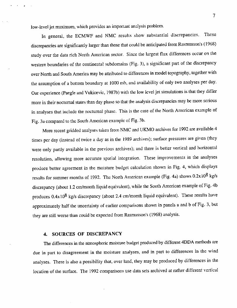
In general, the ECMWF and NMC results show substantial
7
discrepancies. These
discrepanciesaresignificantlylargerthanthosethatcouldbeanticipatedfrom Rasmusson's(1968)
study over the datarich North American sector. Since the largest flux differences occur on the
western boundaries of the continental subdomains (Fig. 3), a significant part of the discrepancy
over North and South America may be attributed to differences in model topography, together with
the assumption of a bottom boundary at 1000 mb, and availability of only two analyses per day.
Our experience (Paegle and Vukicevic, 1987b) with the low level jet simulations is that they differ
more in their nocturnal states than day phase so that the analysis discrepancies may be more serious
in analyses that include the nocturnal phase. This is the case of the North American example of
Fig. 3a compared to the South American example of Fig. 3b.
More recent gridded analyses t_en from NMC and UKMO archives for 1992 are available 4
times per day (instead of twice a day as in the 1989 archives); surface pressures are given (they
were only partly available in the previous archives); and there is better vertical and horizontal
resolution, allowing more accurate spatial integration. These improvements in the analyses
produce better agreement in the moisture budget calculation shown in Fig. 4, which displays
results for summer months of 1992. The North American example (Fig. 4a) shows 0.2xlO 8 kg/s
discrepancy (about 1.2 cm/month liquid equivalent), while the South American example of Fig. 4b
produces 0.4x10⁸ kg/s discrepancy (about 2.4 cm/month liquid equivalent). These results have
approximately half the uncertainty of earlier comparisons shown in panels a and b of Fig. 3, but
they are still worse than could be expected from Rasmusson's (1968) analysis.
4. SOURCES OF DISCREPANCY
The differences in the atmospheric moisture budget produced by different 4DDA methods are
due in part to disagreement in the moisture analyses, and in part to differences ill the wind
analyses. There is also a possibility that, over land, they may be produced by differences in the
location of the surface. The 1992 comparisons use data sets archived at rather different vertical
8
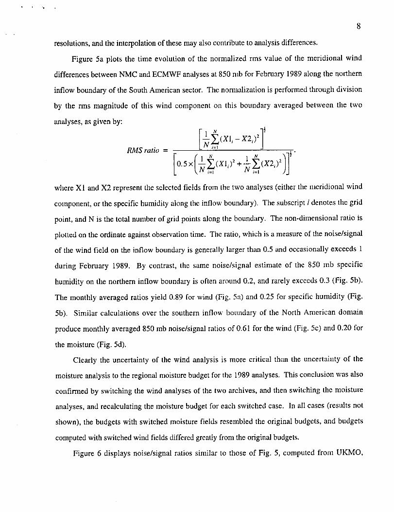
resolutions,andtheinterpolationof thesemayalsocontributeto analysisdifferences.
Figure 5a plots the time evolution of the normalizedrms value of the meridional wind
differencesbetweenNMC andECMWF analysesat 850mb for February1989along thenorthern
inflow boundaryof theSouthAmericansector. Thenormalizationis performedthroughdivision
by the rms magnitude of this wind componenton this boundary averagedbetween the two
analyses,asgivenby:
(XI i - X2i) 2
RAIS ratio = =
where XI and X2 represent the selected fields from the two analyses (either the meridional wind
component, or the specific humidity along the inflow boundary). The subscript i denotes the grid
point, and N is the total number of grid points along the boundary. The non-dimensional ratio is
plotted on the ordinate against observation time. The ratio, which is a measure of the noise/signal
of the wind field on the inflow boundary is generally larger than 0.5 and occasionally exceeds 1
during February 1989. By contrast, the same noise/signal estimate of the 850 mb specific
humidity on the northern inflow boundary is often around 0.2, and rarely exceeds 0.3 (Fig. 5b).
The monthly averaged ratios yield 0.89 for wind (Fig. 5a) and 0.25 for specific humidity (Fig.
5b). Similar calculations over the southern inflow boundary of the North American domain
produce monthly averaged 850 mb noise/signal ratios of 0.61 for the wind (Fig. 5c) and 0.20 for
the moisture (Fig. 5d).
Clearly the uncertainty of the wind analysis is more critical than the uncertainty of the
moisture analysis to the regional moisture budget for the 1989 analyses. This conclusion was also
confirmed by switching the wind analyses of the two archives, and then switching the moisture
analyses, and recalculating the moisture budget for each switched case. In all cases (results not
shown), the budgets with switched moisture fields resembled the original budgets, and budgets
computed with switched wind fields differed greatly from the original budgets.
Figure 6 displays noise/signal ratios similar to those of Fig. 5, computed from UKMO,

9
NMC analysesfor Februaryand July 1992. Over the northern inflow boundary of tile South
Americanregion (Figs. 6a,6b) monthly averagedl_oise/signalratiosare .63 for the wind and .4
for the specific humidity. The correspondingratiosover the southerninflow boundary of the
North Americanregion (Figs. 6c and6d) are .33 for the wind and.16 for the specific humidity.
Wind analysesshowsubstantiallybetteragreementthanin theearlierECMWF andNMC analyses,
but therelative uncertaintyin thewind analysisis significantly largerthan theuncertainty in the
moisture.Theseresultssupporttheinferencethatthenoise/signalratioof themoisturebudgetmay
be improvedmorerapidlyby providing betterwind obselwationsandanalysesthanby providing
bettermoisturedata.
Table 2 displaysthe sensitivity of the calculationto the different surfacepressureand the
different numberof archivetimes. This table presentsthezonal flux below 775 mb through the
westernboundaryof eachdomain. This boundaryis theonly locationwherethesurfacepressure
differed by morethan10mbbetweenthetwo analyses.The first and third colunms of the table are
results based on UKMO and NMC analyses, respectively. The results of the second column are
obtained by using the UKMO wind and moisture analyses, but starting the vertical integral from
the surface pressure level given by NMC analyses. In contrast, the fourth column gives the results
of calculations based on NMC wind and moisture analyses, but UKMO surface pressure analyses.
The similarity between the first and second columns, and the third and fourth columns
indicates that tile change in the surface pressure is not a dominant factor in the discrepancy of the
moisture budget. The last column of Table 2 gives the monthly mean flux based on UKMO
analyses, averaged over only those times when NMC archives are available. Comparing column
five with column one it is clear that the biggest change occurs in July and January when there are
five and four times missing, respectively. However, in all months the last column resembles the
first column more closely than the third column, demonstrating that the differing archive
completeness is not a major factor in the time averaged budget differences.
We conclude that a principal source of the budget discrepancy in the moisture analyses is due
to wind analysis uncertainty. The differences associated with moisture analysis, surface pressure

10
analysis,andarchivecompletenessarelessimportant. Closerinspectkmrevealsthat thc budget
discrepanciesincreaseat different times of day, mainly becauseof differencesin tile way the
differentanalysestreatlow-leveldiurnalwind oscillations.Thenext two sectionssununarizethese
results.
5. DIURNAL CYCLES OF MOISTURE BUDGET
Although more recent comparisons of NMC and UKMO analyse,_ for 1992 are closer than
earlier NMC, ECMWF comparisons for 1989, systematic discrepancies persist, especially in tile
diurnal cycles of boundary layer winds. Panels a and b of Fig. 7 show monthly averaged fluxes
integrated over the four boundaries of the South American box for Janu:wy 1992 at 0000 UTC and
1200 UTC, respectively. The direction of the flux reverses between 00(70 UTC and 1200 UTC in
both analyses on 3 walls (west, north, and east). The net flux convergeace integrated around the
complete boundary reverses as a consequence from outflow at 0000 UTC to inflow at 1200 UTC.
As noted by Rasmusson (1968), calculations of atmospheric moisture flux based upon only
one observation per day can be greatly misleading. On O_e northern inflow bouadary the NMC-
UKMO difference of the diurnal cycle is about 0.8x10⁸ kg/s, or 5 cm/month liquid water
equivalent. This discrepancy is almost as great as the difference between monthly averaged NMC
and ECMWF analyses for the net inflow across all four boundaries for all available times in
February 1989 as shown in Fig. 3. The fluxes averaged over all analysis times (Fig. 4b) do not
reflect such large discrepancies because of fortunate cancellation of similar differences at other
boundaries and times. Because of the systematic differences at different times, the moisture budget
is not much better determined than in the earlier 1989 analyses.
Over North America (Fig. 8) the diurnal oscillation is most conspicuous between 0000 UTC
and 0600 UTC, especially on the southern boundary of the NMC analysis, which has 0.85x10⁸
kg/s more influx at 0600 UTC than at 0000 UTC. The net flux divergence also displays larger
discrepancies at individual times which largely cancel in the complete res'dt of Fig. 4a.
11
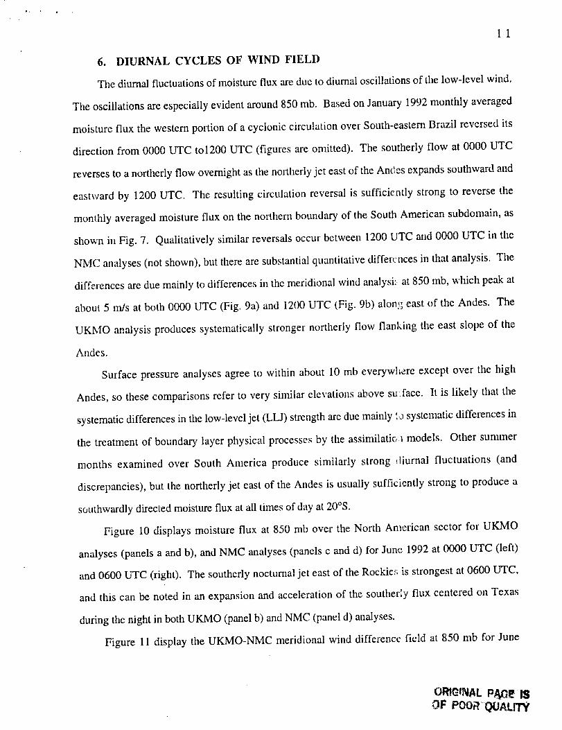
6. DIURNAL CYCLES OF WIND FIELD
The diurnal fluctuations of moisture flux are due to diurnal oscillations of tile low-level wind.
The oscillations are especially evident around 850 rob. Based on January 1992 monthly averaged
moisture flux the western portion of a cyclonic circulation over South-eastern Brazil reversed its
direction from 0000 UTC to1200 UTC (figures are omitted). The southerly flow at 0000 UTC
reverses to a northerly flow overnight as the northerly jet east of the Andes expands southward and
eastward by 1200 UTC. The resulting circulation reversal is sufficicntly strong to reverse the
monthly averaged moisture flux on the northern boundary of the South American subdomain, as
shown in Fig. 7. Qualitatively similar reversals occur between 1200 UTC and 0000 UTC in the
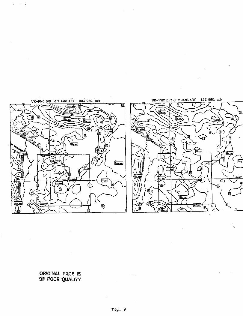
NMC analyses (not shown), but there are substantial quantitative differences in that analysis. The
differences are due mainly to differences in the meridional wind analysi'.-: at 850 rob, which peak at
about 5 m/s at both 0000 UTC (Fig. 9a) and 1200 UTC (Fig. 9b) alon,q east of the Andes. The
UKMO analysis produces systematically stronger northerly flow flanking the east slope of the
Andes.
Surface pressure analyses agree to within about 10 mb everywhere except over the high
Andes, so these comparisons refer to very similar elevations above su.face. It is likely that the
systematic differences in the low-level jet (LLJ) strength are due mainly ',_ systematic differences in
the treatment of boundary layer physical processes by the assimilatic, a models. Other summer
months examined over South America produce similarly strong _liurnal fluctuations (and
discrepancies), but the northerly jet east of the Andes is usually sufficiently strong to produce a
southwardly directed moisture flux at all times of day at 20°S.
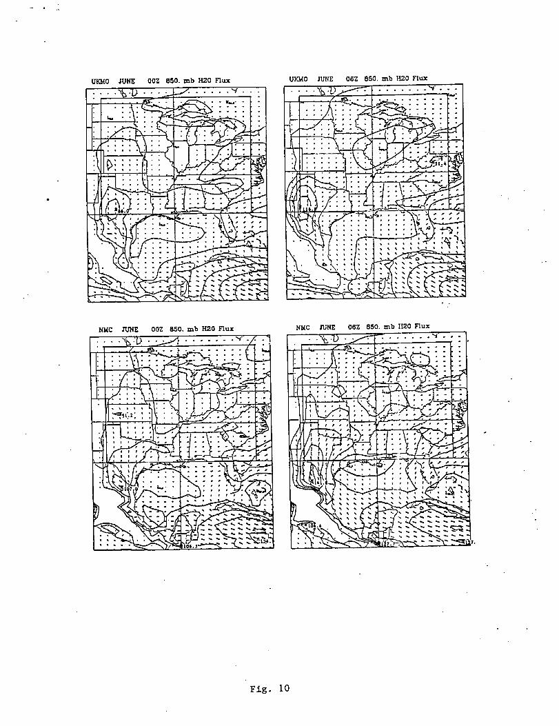
Figure 10 displays moisture flux at 850 mb over the North American sector for UKMO
analyses (panels a and b), and NMC analyses (panels c and d) for June 1992 at 0000 UTC (left)
and 0600 UTC (right). The southerly nocturnal jet east of the Rockie_'; is strongest at 0600 UTC,
and this can be noted in an expansion and acceleration of the southerly flux centered on Texas
during the night in both UKMO (panel b) and NMC (panel d) analyses.
Figure 11 display the UKMO-NMC meridional wind difference field at 850 mb for June
Oi e=fNAL iSOF POORQUALI'I' '
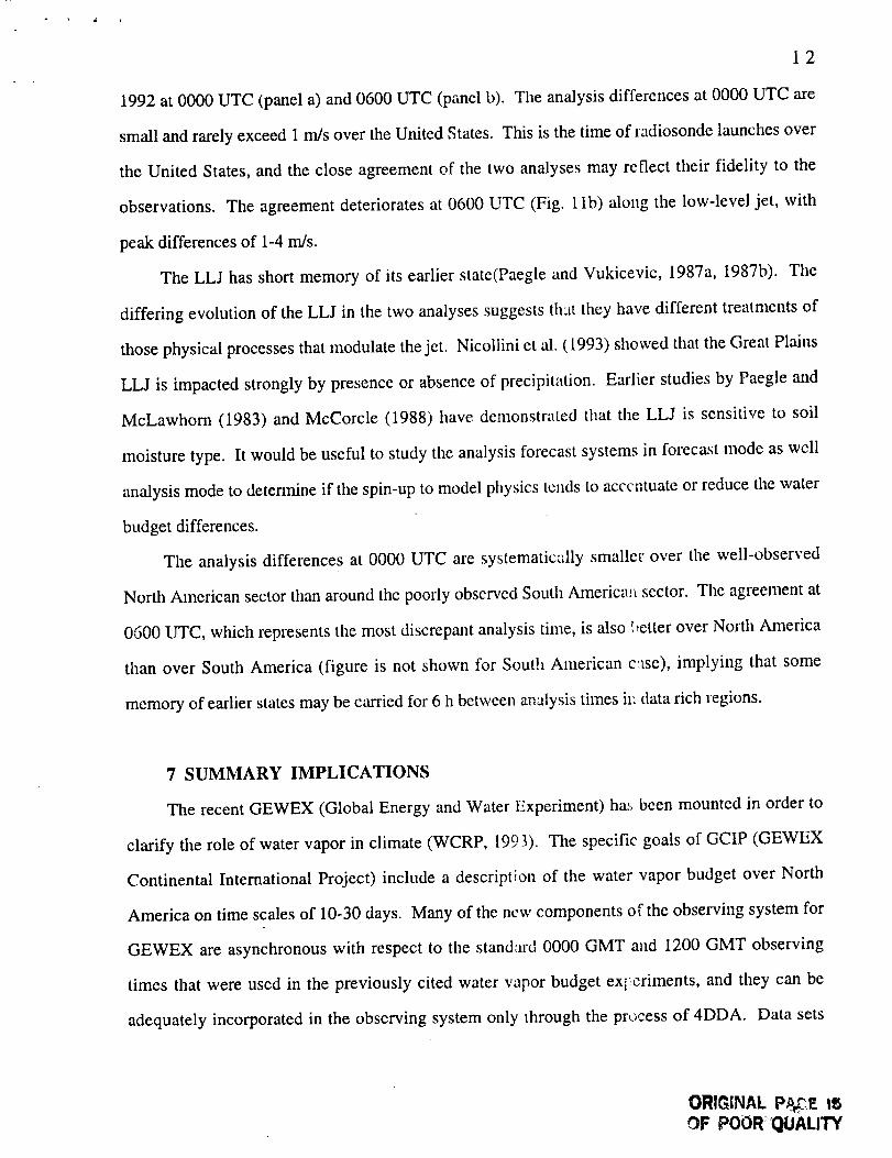
12
1992 at 0000 UTC (panel a) and 0600 UTC (panel b). The analysis differences at 0000 UTC are
small and rarely exceed 1 m/s over the United States. This is the time of radiosonde launches over
the United States, and the close agreement of the two analyses may reflect their fidelity to the
observations. The agreement deteriorates at 0600 UTC (Fig. 1 lb) along the low-level jet, with
peak differences of 1-4 rrgs.
The LLJ has short memory of its earlier state(Paegle and Vukicevic, 1987a, 1987b). The
differing evolution of the LLJ in the two analyses suggests that they have different treatments of
those physical processes that modulate the jet. Nicollini et al. (1993) showed that the Great Plains
LLJ is impacted strongly by presence or absence of precipitation. Earlier studies by Paegle and
McLawhorn (1983) and McCorcle (1988) have demonstrated that the LLJ is sensitive to soil
moisture type. It would be useful to study the analysis forecast systems in forecast mode as well
analysis mode to determine if the spin-up to model physics tends to accentuate or reduce the water
budget differences.
The analysis differences at 0000 UTC are systematically smaller over the well-observed
North American sector than around the poorly observed South Americat sector. The agreement at
0600 UTC, which represents the most discrepant analysis time, is also I,etter over North America
than over South America (figure is not shown for South American c_se), implying that some
memory of earlier states may be carried for 6 h between analysis times il: data rich regions.
7 SUMMARY IMPLICATIONS
The recent GEWEX (Global Energy and Water Experiment) ha. _, been mounted in order to
clarify the role of water vapor in climate (WCRP, 1993). The specific goals of GCIP (GEWEX
Continental International Project) include a description of the water vapor budget over North
America on time scales of 10-30 days. Many of the new components o_"the observing system for
GEWEX ate asynchronous with respect to the standard 0000 GMT and I200 GMT observing
times that were used in the previously cited water w_por budget exl_criments, and they can be
adequately incorporated in the observing system only through the process of 4DDA. Data sets
ORIGINAL P._C,E i_
OF POOR _JALITY

13
pr_:duced by 4DDA are much more commonly used in current large scale diagnostics than are
st :ion data and analyses derived at standard observing times as in the case of the MIT General
C ::culation Data Library. The method of 4DDA has potential shortcomings which have been
pt _tcd out by many investigators. One of these is that certain key elements of the circulation
det!t_ced from observations assimilated in this fashion are more strongly dependent upon the
a1_alysis model used than upon the available observations. This has been shown by
ir_.:rcomparisons of different operational and research data sets by Paegle et al. (1986), Trenbcrth
ar.i Glson (1988) and Trenberth (1991).
The purpose of this investigation has been to present early est;mates of the atmospheric
p_ tions of the hydrology cycle based upon operational data sets produced through 4DDA. One of
tl'_ study regions covers the area east of the Rocky Mountains, which was studied in the series of
ra_!_osonde station data investigations by Rasmusson and is of particular concern to GCIP.
Regional diagnoses of the water vapor budget for selected summer mouths of 1989 suggest more
p .sinfistic conclusions for monthly averaged flux divergence estimates of the atmospheric portion
of the hydrological cycle than those given by Rasmusson (1968) in the sense that NMC and
ECMWF analyses produce monthly differences of the flux of water vapor that are equivalent to E-
P t;ncertainties on the order 7 cmhnonth over South America, and about 3 cm/month over the
ear,tern United States.
Other analyses using these 4DDA data sets are certainly not invalidated by our results. Roads
et al., (1994), for example, corrected for problems at the poorly defined lower boundary by using
a ailable estimates of topography height. Matsuyama et al. (1992) adjusted the ECMWF
d! ,'ergence to conform with streamflow information. These tactics have not been used here
be::ause we simply wanted to determine how reliable the atmospheric analyses are independent of
other information.
Some of these difficulties are related to problems of interpolatio1'_ of the sigma level data to
i:., z'_sure levels (Trenberth, 1991), and to inconsistent handling of l!_e surface pressure. The
i_r_pact of these uncertainties is examined by comparing more highly re.;olved and physically more
14
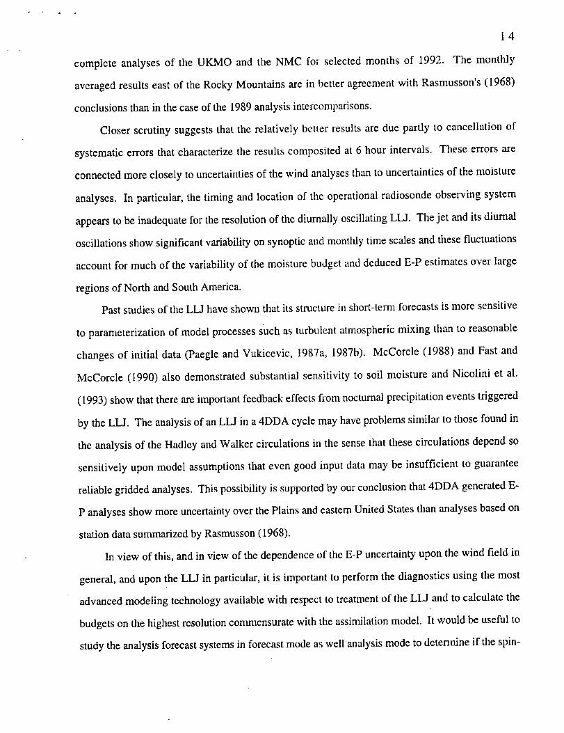
complete analysesof the UKMO and the NMC for selectedmonthsof 1992. The monthly
averagedresultseastof the RockyMountainsarein betteragreementwith Rasmusson's(1968)
conclusionsthanin thecaseof the 1989analysisintercomparisons.
Closerscrutiny suggeststhat the relatively better resultsaredue partly to cancellationof
systematicerrors that characterizethe resultscompositedat 6 hour intervals. Theseerrors are
connectedmorecloselyto uncertaintiesof thewind analysesthanto uncertaintiesof themoisture
analyses. In particular, the timing andlocation of the operationalradiosondeobservingsystem
appearsto be inadequatefor theresolutionof thediurnally oscillatingLLJ. Thejet andits diurnal
oscillationsshowsignificantvariability on synopticandmonthlytime scalesandthesefluctuations
accountfor muchof thevariability of themoisturebudgetanddeducedE-P estimatesover large
regionsof NorthandSouthAmerica.
Paststudiesof theLLJ haveshownthat its structurein short-termforecastsis moresensitive
to parameterizationof modelprocessessuchasturbulentatmosphericmixing than to reasonable
changesof initial data (Paegleand Vukicevic, 1987a,1987b). McCorcle (1988) and Fastand
McCorcle (1990) also demonstratedsubstantialsensitivity to soil moisture and Nicolini et al.
(1993)showthatthereareimportantfeedbackeffectsfrom nocturnalprecipitationeventstriggered
by theLLJ. The analysisof anLLJ in a4DDA cyclemayhaveproblemssimilar to thosefoundin
the analysisof the HadleyandWalker circulationsin thesensethat thesecirculations dependso
sensitivelyuponmodel assumptionsthat evengoodinput datamay be insufficient to guarantee
reliablegriddedanalyses.This possibilityis supportedby ourconclusionthat4DDA generatedE-
P analysesshowmoreuncertaintyoverthePlainsandeasternUnitedStatesthananalysesbasedon
stationdatasummarizedby Rasmusson(1968).
In view of this, andin view of thedependenceof theE-Puncertaintyuponthewind field in
general,andupontheLLJ in particular, it is importantto performthe diagnosticsusingthe most
advancedmodelingtechnologyavailablewith respectto treatmentof theLLJ andto calculatethe
budgetson thehighestresolutionconmaensuratewith theassimilationmodel. It would beusefulto
studytheanalysisforecastsystemsin forecastmodeaswell analysismodeto determineif thespin-

15
up to modelphysicstendsto accentuateorreducetilewaterbudgetdifferences.
Acknowledgments: This researchwas partly funded by NSF grants ATM9014650,
ATM911433,NOAA grantsNA36GP029601andNA56GP0175,andNASA contractS12871Fto
theUniversityof Utah. JuliaNoguesPaegleandAndrewLorenchelpedwith dataacquisitionand
gaveuseful commentsduring the study. Threeanonymousreviewershavehelped improve the
clearityof thepaper.

16
REFERENCES
Fast, J. D., and M. D. McCorcle, 1990: A two-dimensional numerical setlsitivity study of tile great
plains low-level jet. Mon. Wea. Rev., 118, 151-163.
GEWEX Cloud System Science Team, 1993: The GEWEX Cloud System Study (GCSS). Bull of
Amer. Meteor. Soc, 74, 387-399.
Hastenrath, S. L., 1966: The flux of atmospheric water vapor over the Caribbean sea and the gulf
of Mexico. J. of Appl. Meteor., 5, 778-788.
Matsuyama, H., 1992: The water budget in the Amazon river basin duiing tile FGGE period. J.
Meteor. Soc. Japan, 70, 1071 - 1084.
Matsuyama, H., T. Oki, M. Shinoda and K. Masuda, 1994: The seasonal change of the Congo
River Basin. J. Meteor. Soc. Japan, 72, 281-299.
McCorcle, M. D., 1988: Simulation of surface-moisture effects on the great plains low-level jet.
Mon. Wea. Rev., 116, 1705--1720
Nicolini, M., K. M. Waldron, and J. Paegle, 1993: Diurnal oscillations ,.,f low-level jets, vertical
motion, and precipitation: a model case study. Mon. Wea. Rev. 121, 2538-2610.
Paegle, J. and D. W. McLawhorn, 1983: Numerical modeling of diurnal convergence oscillations
above sloping terrain. Mort. Wea. Rev., 111, 67--85.
Paegle, J., W. E. Baker and J. N. Paegle, 1986: The analysis sensitivity to tropical winds from the
global weather experiment. Mon. Wea. Rew., 114, 991-1007.
Paegle, J., and T. Vukicevic, 1987a: The analysis and forecast sensitivity of low-level mountain
flows to input data. Preprints, Fourth Conf. on Mountain Meteorology, Seattle, Amer. Meteor.
Soc., 168--174.
Paegle, J., and T. Vukicevic, 1987b: On the predictability of low-level flow during ALPEX.
Meteor. Atmos. Phys., 36, 45--60.
ORtGINAL p._,Q_i_ IS
OF POOR QUALITY

i7
Rasmusson, E. M., 1966a: Diurnal variations in the summer water v_:por transport over North
America. Water Resour. Res., 2, 469-477.
Rasmusson, E. M., 1966b: Atmospheric water vapor transport an_! the hydrology of North
America. Report No. A-l, Planetary Circulations Project, Massachussc_ts Institute of Technology,
170pp
Rasmusson, E. M., 1967: Atmospheric water vapor transport and the water balance of North
America, Part I. characteristics of the water vapor flux field, Mort. We_,. Rev., 95, 403-426.
Rasmusson, E. M., 1968: Atmospheric water vapor transport and the water balance of North
America, Part II. Large-scale water balance investigations. Mort. Wea. Rev., 96, 720-734.
Roads, J. O., S-C. Chen, A. K. Guetter, and K. P. Georgakakos, 1994: Large-scale aspects of
the United States hydrologic cycle. Bull. Amer. Meteor. Sot., 75, 1589-1610
Rosen, R. D., D. A. Salstein, and J. P. Peixoto, 1979: Variability in the annual fields of large-
scale atmospheric water vapor transport. Mort. Wea. Rev., 114, 2352-2362.
Rosen, R. D., and A. S. Omolayo, 1981: Exchange of water vapor between land and ocean in the
northern hemisphere. J. Geophys. Res., 86, 12147-12152.
Trenberth, K. E. and J. G. Olson, 1988: An evaluation and intercompz_rison of Global analyses
from tile National Meteorological Center and the European Centre for Medium Range Weather
Forecasts. Bull of Amer. Meteor. Soc., 69, 1047-1057.
Trenberth K. E., 1991: Climate diagnostics from global analyses: conservation of mass in
ECMWF analyses. J. of Climate, 4, 707-722.

FIGURE CAPTIONS
Figure 1 Computational domains (boxes) of (a) North American sector and (b) South American
sector. Contours show the orography based on NMC analyses. Contour interval is 250 meters.
Figure 2 Time series of moisture flux divergence over (a) North American sector for July, 1989,
and (b) over South American sector for February 1989. Units in the diagram are 108 kg/s. Solid
lines are the results obtained from NMC analyses, and dashed lines from ECMWF analyses.
Figure 3 Monthly averaged moisture flux and flux divergence for (a) North America (July 1989),
and (b) South America (February 1989). Units are 108 kg/s. Hatched arrows indicate the results
based on ECMWF analyses, and blank arrows indicate the results based on NMC analyses.
Figure 4. As in Fig. 3 for (a) June and (b) January 1992 over North and South America,
respectively. Units are 108 kg/s. Hatched arrows indicate the results based on UKMO analyses,
and blank arrows indicate the results based on NMC analyses.
Figure 5. Normalized rms ratio of analysis differences between NMC and ECMWF for 1989 case.
Rms ratios of (a) wind and (b) specific humidity analyses over South American inflow boundary
for February, 1989. Similarly rms ratios of (c) wind and (d) specific humidity for North American
inflow boundary for July 1989.
Figure 6. As in Fig. 5 for 1992 case: (a) South America Fcbruary 1992 wind analysis, (b) South
America February 1992 specific humidity analyses, (c) North America July 1992 wind analyses,
and (d) North America July 1992 specific humidity analyses.
Figure 7 Monthly mean moisture flux and flux convergence averaged over (a) 0000 UTC, and (b)
1200 UTC for January 1992 over South America. Hatched arrows indicate results based on
UICMO analyses, and blank arrows indicate results based on NMC ana!ims. Units are 108 kg/s.
Figure 8 Monthly mean moisture flux and flux divergence averaged over (a) 0000 UTC, and (b)
0600 UTC for June 1992 over North America. ttatched arrows indicate the results based on
UFAVIO analyses, and blank arrows indicate the results base.! on NMC analyses. Units are 108
kg/s.
ORIGINAL P_E iSOF POOR =_UALiTY
Figure 9 Monthly mean 850 mb meridional wind difference between UKMO and NMC analyses
averaged at (a) 0000 UTC, and (b) 1200 UTC. Negative contours are d;_shed. Contour interval is
I m/s.
Figure 10 Monthly averaged moisture flux (vq dp/g) at 850 mb for North America June 1992
based on UKMO analyses, (a) and (b), and NMC analyses (c) and (d). Left panels are averaged at
0000 UTC, and right panels averaged over 0600 UTC. Contour interval is 25 kg/ms.
Figure 11 Monthly mean 850 meridional wind difference between U_VIO and NMC _malyses
averaged at (a) 0000 UTC, and (b)0600 UTC over North America. Negative contours are dashed.
Contour interval is 1 m/s.
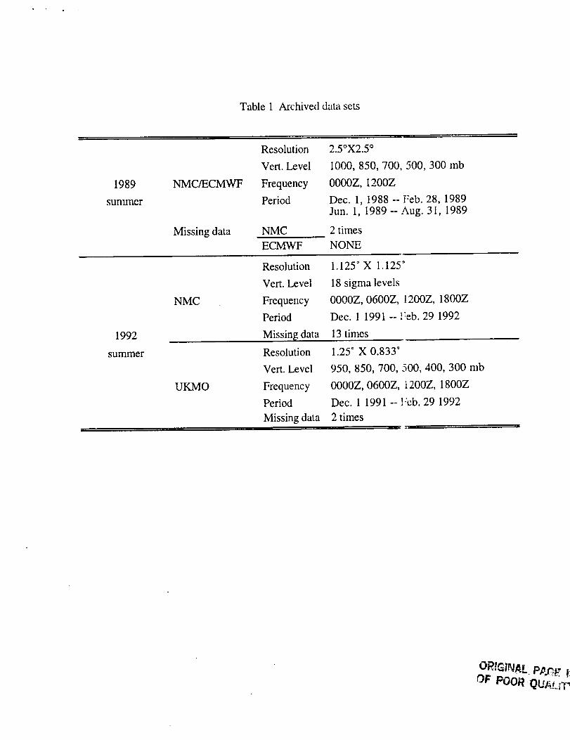
Table1 Archiveddatasets
1989
summer
NMC_CMWF
Missingdata
Resolution
Vert.Level
FrequencyPeriod
NMCEC_
2.5°X2.5°
I000, 850, 700, 500, 300 mb
0000Z, 1200Z
Dec. 1, I988--Feb. 28, 1989
Jun. 1, 1989--Aug. 31, 1989
2 times
NONE
1992
summer
NMC
Resolution
Vert. Level
Frequency
Period
Missin_ data
UKMO
Resolution
Vert. Level
Frequency
Period
Missing data
1.125" X 1.125 °
18 sigma levels
0000Z, 0600Z, 1200Z, 1800Z
Dec. 1 1991 -- Feb. 29 1992
13 times
1.25" X 0.833*
950, 850, 700, 500, 400, 300 mb
0000Z, 0600Z, _200Z, 1800Z
Dec. 1 1991 -- !:cb. 29 1992
2 times
oF Poor

South
America
North
America
Table 2 Moisture fluxe through the western boundary
over North and South American sectors. (1000-775 mb) Unit: 108 kg/s.
i
UKMO UKMO NMC NMC UKMO
NMC_sfp UKMO_sfp part
December -0.3254 -0.2832 0.0393 0.0423 -0.3260
January -0.5401 -0.6034 -0.3590 -0.3506 -0.5560
February -0.4494 -0.5125 -0.0672 -0.0621 -0.4494
June -0.0468 -0.0966 -0.1023 -0. !045 -0.0526
July 0.2233 0.1615 0.0787 0. 1222 0.1994
August 0.0151 -0.0197 -0.0305 0.0393 0.0161 _,.

_0_120°W
IIII
...........................•.90°W
)ON
O°N
_Q
_O°S
...................... _O°S
60°WCONTOUR FROM 250 TO 4750 BY 250
Fig. I

v 4
'- 2v
_0
_>-2
8-4=x-6ii"
6
_(a)
_'..... ,,,, I,,, , I,,,, I h,v,, t
0 5 10 15 20 25 30
July 1989
_4_2_P
=0
_'-2"-40o
×-6n-
•(b) / '/ \/I '_
s I t i l i r i I I l l _,,l l , [ , , I _ , _ , .I , L l I
0 5 10 15 20 25
February 1989
3O
Fig. 2

(a)
0.44 IZ
0.72 <
0.11 0.45
Y/Ill
1.99 1.54
"//l///J'_ 3.01
Total flux convc, gence= -1.15 NMC Outflow= -0.58 ECMW_ Outflow
(b) 2.o2 2.18
0.47
o.26 I
4)0.06 O. 1 6
1.83
Total flux convergence= -0.19 NMC Outflow= 0.99 ECM'_F Inflow
ORIGINAL P6._E IS
OF POOR '(_JALJTY
Fig. 3

1.58
1.40
(a) 0.07 0.12
I
>
1.11 1.26
"////////J_ 2.56
D 2.37
Total flux convergence= 0.20 NMC Inflow= 0.39 UKMO Inflow
(b) 0.23 0.21
0.33 > <
0.21 > [
0.27 0.56
0.14
Total flux convergence-- -0.12 NMC Outflow= 0.13UKMO Inflow
O_gGINAL P_E IS
OF POORQUALITY
Fig. 4

u_

,-. 0
pU!M ;0o!_eJS_I_I
l 0
o4
o
I....
-3
0
0¢'9
14")
o
__L__________oli_ _-- I._ 0,-: d
b ;o o!_eJSI_I
04

(a) 0.48 0.97
0.8S
]
0.22 0.50
< 0.13
Tota_ flux conve_ gence= -0.96 I'¢MC O_ow= -0.67 UKMO Oul:flow
(b) 0.88
0.54
| nV0.25
1.21
0.40
E
0.37
Total flux convergence= 0.64 NMC Inflow= 1.13 UKMO Inflow
Fig. 7

Ca)
1.19
1.27
V V
vIt/ll/x
/,,, /,,,,u H
0.64 1.12
2.33
2.32
Total flux convergence= -0.29 NMC Outf]ow= 0.19 UKMO h'uTow
(b)
1.64
I.40
0.12 0.08
>
I.49 I.48
2.74
_ 2.32
Total flux coi:.vergence= 0.69 NIv[C Inflow,,: 0.45 UKMO hd]ow
Fig. 8
OF POOR 'QUALI't_
_-_c D_fotv _A_u_Y ooz950.,=b UK-_C Dt£tof V 3A//UARY 12Z 950. mb
L _ _ EORIGINAL P_.. ISOF POOR QUALI"i_7
Fig. 9
NI_C JUNE OOZ 850. mb I'L?.OFlux
UI_O JUNE 06Z 850. mb H20 Flux
....... '_r,j" 0 . "1
.: i :: ! 't_iiiii -i
t , , • . -"/. . • _"_ - _' ,.,, • s
•',.._\: : :t: ,/,-:_: .- :_
Fig. i0

i
UK-NMC I_ilf o! Y ,F_JNE (]OZ 8_0. mb
S>:3.
£
IJ_
i
-'h
_.°.,
\.\.
UK-NMC DU. r ,_' V 06Z 850. mb
\
Fig. Ii

,=j ........ L ,.
,Report Documentation Page
-_-. _ _ml i,._d,_, .......
Analyses and Forecosts with LAWS Winds
+-.
t.Aut_d
Jan Paegle
..•d
o. _,,_ =_,_._,_ re,m,,_£;,,,_,,.. "'-
University of Utah °
Dept. of MeteorologySalt Lake City, UT 84112
t . , .___ . . .
National. Aeronautics and space Administration
Mail Stop 126
Hampton VA, 23665
ml s_._,n_ _, ............
; ]
l
7-15-95 ' ', .
& h,_r_r_r_r_r_r_r_r_O_.n_n _, No.
11. C.on_e_'to¢ Car_! No+---
Final 9,/22/93 -
12,/ii/9_ .....
p._ ._-/J_/. _
1'6.Al_t.+cl--.. ..- .i
F
See attached sheet.
p
+
I
, Space-based winds hydrologic cyclei
111.I)kulb.tt=_ Su,om_mt
21. He, _i=
ORtGINAL P,c_B IS+-_,cPO0_ QUALITY
22. p,_;_,'
• il . 1 i ll .... , .... I __ 11 _ . i f l .... I . I
NASA I_RM 1_ OCT I_