e wall/wake ble layers - nasa wall/wake ble layers (nasa-cr-4286) ... stokes code using the...
TRANSCRIPT

e Wall/Wake
ble
Layers
(NASA-CR-4286) DEV_cLOPMENT OF: A DEC£CT
STREAM !::UNCI'ION, LAW OF [HE WALL/WAKE METHO0
FOR COMPRC_SS[BLF_ TURBULENT BOUNDARY LAYFR$
Ph.D. Thesis (North Carolina State Univ.)
25 p CSCL 20D
https://ntrs.nasa.gov/search.jsp?R=19900009359 2018-05-23T00:00:40+00:00Z

_,_ rrl n _rT]mmln - arm
L .
• 7"-'--- -
• " _ .......... L ...... --
F
ak_
__ ...... _ _ _
NASA Contractor Report 4286
Development of a Defect Stream
Function, Law of the Wall/Wake
Method for Compressible
Turbulent Boundary Layers
Richard A. Wahls
North Carolina State University
Raleigh, North Carolina
Prepared for
Langley Research Center
under Cooperative Agreement NCC1-117
National Aeronautics andSpace Administration
Office of Management
Scientific and TechnicalInformation Division
1990


Abstract
WAHLS, RICHARD A. Development of a Defect Stream Function, Law of the
Wall/Wake Method for Compressible Turbulent Boundary Layers (Under the direction of
Dr. Fred R. DeJamette)
The method presented is designed to improve the accuracy and computational
efficiency of existing numerical methods for the solution of flows with compressible
turbulent boundary layers. A compressible defect stream function formulation of the
governing equations assuming an arbitrary turbulence model is derived. This formulation
is advantageous because it has a constrained zero-order approximation with respect to the
wall shear stress and the tangential momentum equation has a first integral. Previous
problems with this type of formulation near the wall are eliminated by using empirically
based analytic expressions to define the flow near the wall. The van Driest law of the wall
for velocity and the modified Crocco temperature-velocity relationship are used. The
associated compressible law of the wake is determined and it extends the valid range of the
analytic expressions beyond the logarithmic region of the boundary layer. The need for an
inner-region eddy viscosity model is completely avoided. The near-wall analytic
expressions are patched to numerically computed outer region solutions at a point
determined during the computation. A new boundary condition on the normal derivative of
the tangential velocity at the surface is presented; this condition replaces the no-slip
condition and enables numerical integration to the surface with a relatively coarse grid using
only an outer region turbulence model. The method has been evaluated for incompressible
and compressible equilibrium flows and has been implemented into an existing Navier-
Stokes code using the assumption of local equilibrium flow with respect to the patching.
The method has proven to be accurate and efficient.
iii
4 B
PRECEDING PAGE BLANK NOT FILMED _ 1 [ INTENTIONAI_.¥BLANI[-

Acknowledgements
The author would like to thank Dr. Richard W. Barnwell, Chief Scientist of NASA
Langley Research Center, and Dr. Fred R. DeJarnette, Professor of Mechanical and
Aerospace Engineering at North Carolina State University, for their time and effort during
this investigation. The guidance and interest of these two men was invaluable to the
research effort and very much appreciated by the author.
The author also appreciates the opportunity to work with and learn from the faculty
at North Carolina State University and the staff of the Computational Methods Branch at
NASA Langley Research Center. In particular, the author would like to thank Dr. David
H. Rudy and Dr. Ajay Kumar of the Computational Methods Branch for their interest and
assistance; and Dr. Hassan A. Hassan and Dr. Richard E. Chandler of North Carolina State
University for their participation on the author's doctoral advisory committee.
Support for this investigation was provided by the Computational Methods Branch
of the Fluid Mechanics Division at NASA Langley Research Center through Cooperative
Agreement NCC 1-117.
iv

Table of Contents
Page
LIST OF TABLES .................................................................................. vii
LIST OF FIGURES ............................................................................... viii
1. INTRODUCTION .......................................................................... 1
2. DEFECT STREAM FUNCTION FORMULATION .................................. 13
2.1 Basic Equations .................................................................... 13
2.2 Law of the WaU and Wake ....................................................... 17
2.3 Shear-Stress Velocity Ratio ...................................................... 19
2.4 Governing Equations ............................................................. 21
2.5 Boundary Conditions ............................................................. 22
2.6 First Integral of Governing Equation ........................................... 24
2.7 Zero-Order Approximation ....................................................... 27
2.8 Equilibrium Flow Approximation ............................................... 28
3. INNER REGION TREATMENT ........................................................ 31
3.1 Equation Relating f and f'. ....................................................... 32
3.2 Match Point Location ............................................................. 33
3.3 Implementing the Inner Region Treatment ..................................... 34
4. RESULTS AND DISCUSSION ......................................................... 39
4.1 Incompressible Flow .............................................................. 39
4.2 Compressible Flow ............................................................... 45
4.3 Primitive Variable Application ................................................... 52
5. CONCLUDING REMARKS ............................................................. 58
V

J
o
8.
9.
APPENDICES .............................................................................. 60
6.1 Appendix A: Analytic Solution for Compressible Turbulent Flow ......... 60
6.2 Appendix B: Analytic Solution for Incompressible Turbulent Flow
at 13= -0.5 .......................................................... 63
REFERENCES ............................................................................. 65
TABLES ..................................................................................... 69
FIGURES ................................................................................... 72
vi

List of Tables
Table 1.
Table 2.
Table 3.
Shear-stress velocity comparisons with experimental dataand analytical solutions for incompressible flow.
Shear-stress velocity ratio comparisons of constrained zero-orderand full equation equilibrium solutions.a) The effect of Me variations.
b) The effect of Res. variations.A
c) The effect of 13variations.
Shear-stress velocity comparisons with experimental dataand analytical solutions for compressible flow.
Page
69
70
70
70
71
vii
List of Figures
Figure 1.
Figure 2.
Figure 3.
Figure 4.
Figure 5.
Figure 6.
Figure 7.
Figure 8.
Figure 9.
Figure 10.
Page
Laminar and turbulent velocity profiles on a flat plate.(reprint from reference 11)
72
Laminar-like behavior of the outer region of turbulent boundary layers.(composite of reprints from reference 31)a) Several experimental turbulent velocity prof'des on flat plates. 73b) Universal plot of experimental turbulent velocity profiles on flat plates. 73c) Solutions of the Blasius equation with nonzero surface velocities. 74d) Comparison of the data shown in fig. 2b and 2c. 74
Velocity defect profiles with [3 = -0.5 for incompressible flow. 75
Grid resolution comparison for incompressible flow. 76
Velocity defect profiles with 13-< 1 for incompressible flow.
a) [3 = 0 77
b) [3 = 0.5 78
c) 13= 1 79
Velocity defect profiles with 13> 1 for incompressible flow.
a) 13= 4,/3 80
b) 1] - 2 81
c) _ = 4 82
d) 13= 10 83
Effect of the Clauser constant k on convergence with 13= 10
for incompressible flow. 84
Shear-stress velocity ratio comparison with Re_5* = 105
for incompressible flow. 85
Inner variable profiles for several incompressible cases.
a) Computational comparison with 13= 4 and Re_5* = 105. 86
b) Comparison with experimental data with 13= 7.531 and Res* = 30,692.5.87
A
Effect of Me on the velocity defect profiles with 13= 0 and Res* = 104. 88
viii
Figure 11.
Figure 12.
Figure 13.
Figure 14.
Figure 15.
Figure 16.
Figure 17.
Figure 18.
Figure 19.
Figure 20.
Figure 21.
Figure 22.
A
Effect of Res* on the velocity defect profiles with Me = 3 and 13= 0. 89
A
Effect of 13on the velocity defect profiles with Me = 3 and Res* = 104. 90
Analytic and numeric values of the law of the wake withA
13= 0 and Reso = 104. 91
Behavior of the the law of the wake coefficient.^
a) Effect of 13and Me with Res* = 104.
b) Effect of Res° and Me for flat plate flow.
92
93
The incompressible law of the wake coefficient.
a) Comparison of analytical and numerical values of II.
b) Comparison of analytical and numerical values of w.
94
95
A
Effect of 13on the law of the wake coefficient exponent 0_. 96
Grid resolution comparison for compressible flow. 97
^
Effect of 13on various profiles with Me = 3 and Res* = 104.
a) Effect on velocity defect profiles.b) Effect on velocity profiles.c) Effect on density profiles.
9899
100
Effect of Me
a) Effect onb) Effect onc) Effect on
A
on various profiles with _1= 0 and Res* = 104.
velocity defect profiles.velocity profiles.density profiles.
101102103
Behavior of the shear-stress velocity ratio.^
a) Effect of 13and Me with Res° = 104.
b) Effect of Res° and Me for flat plate flow.
104
105
Trends of the compressibility parameter co.^
a) Effect of 13and Me with Res* = 104.
b) Effect of Res° and Me for flat plate flow.
106107
Comparison of various profiles with experimental data for compressible flowon a flat plate.a) Comparison of velocity defect prof'des. 108b) Comparison of velocity profiles. 109c) Comparison of density profiles. 110
ix
Figure 23.
Figure 24.
Baseline and slip-velocity Navier-Stokes solutions for Me = 2.578.
a) Velocity ratio comparison.b) Density ratio comparison.
Baseline and slip-velocity Navier-Stokes solutions for Me = 4.544.
a) Velocity ratio comparison.b) Density ratio comparison.
111112
113114
X

1 INTRODUCTION
It is generally accepted that turbulence is the most complicated kind of fluid motion.
Many researchers have directed extensive effort towards the physical understanding and
computation of turbulent flows. Turbulence has been described by Hinze 1 as "...an
irregular condition of flow in Which the various quantities show a random variation with
time and space coordinates so that statistically distinct average values can be discerned."
The major problem when attempting to compute a turbulent flowfield from first principles
is that the time and space scales of the turbulent motion are extremely small. The
computational grid required to fully resolve such a flow in this manner are beyond the
limits of todays computer technology. Anderson et al 2 provide an estimate of the spacing
required for a typical flowfield in which "10 5 points may be required to resolve just 1 cm 3
of the flowfield." It is because "statistically distinct average values can be discerned" that
modeling techniques can be developed that allow us to solve turbulent flowfields for
engineering purposes.
Currently there are two basic approaches for computing turbulent flowfields 3. The
first approach is known as a large eddy simulation. This approach attempts to compute the
maximum amount of information about the turbulent motion as it attempts to capture the
turbulence on a real-time, real-space basis. Large eddies, which are responsible for the
majority of the momentum transport, are resolved on the scale of the grid. Subgrid
modeling is used to describe the effects of the small eddies, which cannot be resolved with
practical grids. It has been projected 3 that fully converged large eddy simulations for
simple airfoils is beyond the capability of current computers.
The second, and more prevalent, approach is to calculate the mean motion of the
fluid by use of the time-averaged Navier-Stokes equations. These equations are often
referred to as the Reynolds equations. They are derived by decomposing the dependent

variablesintomeanandfluctuatingcomponentsandthenaveragingtheequationsovertime.
Theresultingequationsareexpressedprimarily in termsof meanvariableswith the
transienteffectsof turbulencebeingdescribedby thefluctuatingquantitiesthatappearin the
turbulentor Reynoldsstressterms;theReynoldsstresstermsrequiremodeling. This
approachdoesnotattemptto capturetheturbulenceonareal-time,real-spacebasisbut
insteadreliesona turbulencemodeltoconveytheeffectsof theturbulentmotionon the
meanflow. Also, the solution schemes do not need to be time accurate and are able to
converge much more rapidly than with large eddy simulations. On the other hand,
information on the dynamics of turbulence is lost. It is fortunate that the simpler statistical
• . 4approach is adequate for general engmeenng purposes .
Turbulence modeling is the most important and most difficult aspect of the statistical
methods. The turbulence model is necessary to mathematically close the system of
governing equations and must fully describe all of the effects of the turbulent motion on the
mean flow. Several excellent review papers on the state of turbulence modeling have been
given by Rubesin 3, Lakshminarayana 5, Marvin 6, and Rubesin and Viegas 7. Turbulence
models can be categorized as either zonal or global in reference to their range validity 3. The
zonal model is one which is designed for a specific application and is usually developed
from this specific class of experiments. In general, these models do an excellent job of
predicting flows of the particular class but begin to lose accuracy and break down when
extending beyond these flows. The global models, however, involve more complex
functions, such as the field equations for the turbulence quantities, and have a wider range
of applicability. The more complex models require more empirically based coefficients
than do the zonal models; these coefficients are determined from more than one class of
experiments. The basic necessity of empirical coefficients restricts the global models from
successfully predicting flows of all types. At present, a true global, or universal, model
2

which is accurate for all flows has yet to be determined. Thus, it can be stated that current
turbulence models are restricted to various zones of application.
Turbulence models can also be classified as either eddy-viscosity or stress-transport
models 6. Eddy-viscosity models rely on the Boussinesq 8 concept, which models the
turbulent shear stress as the product of an effective viscosity and a mean rate of strain. The
effective viscosity is proportional to the velocity and length scales of the turbulence in the
various regions of the flow. Eddy-viscosity models can be further classified according to
the method of determining the effective viscosity; in other words, the various eddy-
viscosity models are functions of the method used to describe the velocity and length scales
of turbulence. They are classified as either zero-, one-, or two-equation models, where the
designation refers to number of field equations used in addition to the usual mean flow
equations. The simplest is, of course, the zero-equation model, which determines the eddy
viscosity based entirely on the properties of the mean flow. The two primary examples of
this type are those of Cebeci and Smith 9 and Baldwin and Lomax 10. These models are
widely used in practical engineering applications for simple shear flows and in many
Navier-Stokes codes 5. The one-equation models typically rely on the solution of the
turbulent kinetic energy equation to represent the velocity scale, and the two-equation
models incorporate the solution of an additional equation which represents the length scale
of the problem. The one- and two-equation models are more general than the zero-equation
models but, in many instances, do not improve the accuracy of the solutions.
The stress-transport models use the Reynolds-stress equations to model turbulence
in the mean flow equations. Here closure is achieved through the solution of the mean
turbulent field and requires the solution of up to six additional differential equations for the
Reynolds stresses, thus significantly increasing the computational effort required beyond
the capability of current computers 5. As a result, several attempts to simplify the stress-
transport equations have been made and are discussed in detail in reference 5. These

approachesmakeassumptions,somearbitraryandothersbasedon thephysicsof theflow,
thatallow thestress-transportequationsto bereducedto analgebraicform. Notethateven
in differentialform,theseequationsstill requiremodelingof severaltermswhich involvea
numberof empiricalcoefficients.Themainadvantagerelativeto eddy-viscositymodelsis
thatthestressesareableto respondimmediatelyto changesin therateof strain.These
modelsareappropriatefor awiderrangeof flow conditionsincludingseparatedand
recirculationregionsfor whicheddy-viscositymodelsarenotvalid.
Thecurrentinvestigationisconcernedwith thesolutionof compressibleturbulent
boundarylayersoversolidsurfaces.Theflowfieldsstudiedarerestrictedto attached
boundarylayersunderadiabaticwall conditions.Theformulationis derivedsuchthatit is
consistentwith theeddy-viscosityconcept.Overtheyears,considerableresearchhasbeen
devotedto thedevelopmentof numericalmethodsforjust suchsituations.The
computationaleffort requiredof thesemethodsis highlydependenton thenumberof grid
pointsnecessaryto accuratelyresolvetheflowfield. Boundary-layerflows in general
requireafinely spacedgrid in orderto accuratelycalculatetheirpropertiesandtheir
influenceon theexternalflow. Turbulentboundarylayers,in particular,demandavery
fine grid nearthewall in orderto resolvethehighgradientsof thephysicalpropertiesin
thisregion;however,amuchcoarsergrid similar to thatnecessaryfor a laminarboundary
layercanbeusedin theouterregionawayfrom thewall. Blottner11presentedanexcellent
exampledemonstratingthedifferentgrid requirementsfor laminarandturbulentboundary
layers.Blottner'sfigureis reproducedherein figure 1. With acommonouteredgeof the
boundarylayerdefinedandtherequirementof onepercentaccuracyof theshearstressat
thewall, Blottnerestimatedthenumberof uniformintervalsnecessaryto resolvelaminar
andturbulentboundarylayerson aflat plate.He foundthattheturbulentprofilerequired
twentytimesthenumberof intervalsasthelaminarprofile. Theadditionalintervals
requiredareadirectresultof thehighgradientregionnearthewall, andto alesserextent,

the increasedthicknessof theturbulentboundarylayer. An obvioussolutionto this
problemis theuseof anonuniformgrid whichclustersgrid pointswherethemost
resolutionis needed;in thiscase,gridpointsareclusteredin thehighgradientregionnear
thewall. Nonuniformgridsarein everydayuseandhavebeenfor manyyears.Despite
this technique,thegridrequirementsstill becomeexcessivewhendealingwithcomplex
two-dimensionalandeventhesimplestthree-dimensionalflowsascomputationaltimecan
takemanyhoursor daysevenon thefastestavailablecomputers.
An additionaltechniquewhichhasbecomepopularrecentlyis theuseof wall
functions. In effect,wall functionsreplacethehighlyclusteredgridpointsand
correspondingnumericalcomputationsnearthesurfacewith empiricallybased,analytic
expressionsfor velocity, temperature,andotherquantitiesasnecessaryfor compatibility
with aparticularturbulencemodel. It is, in fact,thepotentialreductionof computational
effort thatis themainincentivebehindthedevelopmentof wall functiontechniques.
Experimentalinvestigationsof turbulentflows, andthecorrespondinganalytic
investigations,haveestablishedexpressionsfor thenear-wallregionwhichhaveprovento
bequite accurateandrobust.Theuseof suchexpressionsshouldnotbeaconcernasit is
apparentthatall turbulentflow analysesarebasedonempiricismto someextent.The
logarithmiclaw of thewall for velocityisoneof themostwidelyusedandaccepted
expressionsof this type. It is, in fact,oneof themostwidelyacceptedempiricismsin all
of fluid mechanicsandhasprovenusefulevenbeyondtheboundsof its strictassumptions.
Thebasicconceptof thewall functionmethodsis to determineanalyticallythe
flowfield variablesfrom thesurfacetoapoint nearthesurfacewheretheanalytic
descriptionis valid. This is thefirst grid pointoff of thesurface.From thispoint outward,
theflowfield is resolvedwith anappropriatenumericalmethodandassociatedturbulence
model. Theanalyticdescriptionof theflowfield variablesat thefirst grid pointprovides
boundaryconditionsusedto computetheremainderof theflowfield. Mostmethodssimply
5

patchtheanalyticandnumericsolutionsatthispointwhilesome,suchastherecentmethod
of Walker,Fee, and Werle 12, formally match the outer limit of the inner solution to the
inner limit of the outer solution. A common characteristic of current wall function
approaches isthe precomputation designation of the first grid point off of the wall; that is,
the section of the flowfield to be determined analytically is decided prior to the
computation. This characteristic is independent of the numerical method and turbulence
model. The grid point location is crucial because it must be within the range of validity of
the analytic model at all streamwise locations. This grid point is typically chosen to lie
within the viscous sublayer or logarithmic region of the boundary layer. As such, this
approach does not take full advantage of the analytic expressions because their use is
limited to only a portion of their valid range. It follows that near-wall turbulence models
are still required although not to the same extent as without the use of wall functions.
Rubesin's review of turbulence modeling 3 points out several major advantages that
wall function methods have over methods that integrate to the surface. First of all, wall
function methods have proven to be quite economical due to the reduction in the number of
grid points required to resolve the flowfield as well as to the increase in the allowable time
step due to the increased size of the minimum grid spacing. Secondly, present near-wall
turbulence models have inherent physical uncertainties and, in some instances, result in a
numerically stiff set of equations near the surface. The use of the wall functions has been
shown to increase the accuracy of the solutions near the surface in many cases while
relieving this near-wall stiffness. As far as the accuracy is concerned, it should be
advantageous to model the inner region with an empirical representation which can be
validated by direct experimental observation rather than with another model, such as an
eddy-viscosity model, which cannot be validated by direct experimental observation. The
point is that error can enter through a model if said model is based on indirect empiricism

suchasvelocity measurementsbeingcorrelatedandput in theform of aneddyviscosity;
theeddyviscosityis notapropertywhichcanbemeasureddirectly.
Oneof themosteffectivewall functionmethodsto dateis thatof Viegas,Rubesin,
andHorstman13,which is anextensionof themethodoriginallydevelopedby Viegasand
Rubesin14to increasecomputationalefficiencyfor their studyof shockwave/boundary
layerinteractions.Theirmethodhasprovento besuccessfulnotonly by increasingthe
efficiencyof theirsolutionprocedurebyanorderof magnitudewith respectto thecomputer
timepersolution,butalsoby improvingtheaccuracyof theirsolutions.Themethodhas
provensuccessfuloveravarietyof flowfields includingtwo-dimensionalseparatedflows.
However,severalparameters,suchastheskin-frictioncoefficientandshocklocations,
remainsomewhatsensitiveto thechoiceof thefirst gridpointoff of thesurface(thepatch
pointof theanalyticandnumericsolutions).More recentlyWilcox15reportsthesensitivity
of the locationof thefirst gridpointon theskinfriction.
Themethodput forthin this investigationcombinestcaditionalwall functionideas
with featuresdesignedto furtherimprovecomputationalefficiencyandaddresssomeof the
shortcomingsof previousmethods.Theimprovementin efficiencywill beadirectresultof
furthergridreduction,andtheprimaryshortcomingaddressedis thechoiceof the location
of thefirst grid point. Themethodproposedconsiderstheturbulentboundarylayerasa
compositeconsistingof aninnerregionnearthesurfacewith anouterregionbeyond.The
tworegionsaresimilarto thoseencounteredwith zero-equationturbulencemodels,which
useseparateeddy-viscositymodelsin thedifferentregions.Theinnerregionis to be
resolvedin acompletelyanalyticmannerwhile theouterregionis resolvednumerically.
Theinnerregionexploitsthelaw of thewall for velocityin conjunctionwith anassociated
law of thewake. Thelaw of thewakeenablestheeffectsof streamwisepressuregradients
to influencetheregionnearthewall. Theenergyequationis replacedbyamodifiedform
of theCroccotemperature-velocityrelationship.Theouterregionis formulatedand
7

resolvedin termsof thedefectstreamfunction. This formulationproperlycharacterizesthe
outerportionof theboundarylayerasit relatesthelocalmeanvelocityto thevelocityatthe
outeredgeof theboundarylayer.
As statedearlier,thelaw of thewall for velocityis probablythemostwidely
acceptedempiricismin fluid mechanics.Themostcommonform of this law isknownas
thelogarithmiclaw of thewall andisvalid in thefully turbulent,logarithmicregionof the
innerpartof theboundarylayer. Othershavedevisedlawsthatarevalid from thewall
throughtheviscoussublayerandthelogarithmicregion. Onesuchexamplefor
incompressibleflow is the law givenbyLiakopolous16,whichwasusedin aprior
investigation17'18by thepresentauthor.Far andawaythemostpopularcompressiblelaw
of thewall is thatdescribedastheeffective,or generalized,velocity approachof van
Driest19,whicheffectivelyrelatesthevelocityin acompressiblefluid to acorresponding
velocity in anincompressiblefluid. ThevanDriestlaw isusedin thepresentmethodandis
discussedfurther in section2.2.
Law of thewakeempiricismshavenotbeendevelopedor usedto theextentaslaw
of thewall empiricisms,particularlyfor compressibleflows. Themostpopularlaw of the
wakeis thatpresentedby Coles20for incompressibleflow. Moses21alsogivesa
commonlyusedincompressiblelaw of thewake. Severalotherlawsfor incompressible
flow aregivenby White in reference22. McQuaid23proposedanincompressiblelaw that
usedamodifiedshear-stressvelocityasthenormalizingvariable,suchthatpressure
gradientsfrom themostfavorableto separationcouldbehandledwith relativeease,while
themorecommonlawsof thewakesimplyusetheshear-stressvelocityasthenormalizing
variable.Themostpopularform of acompressiblelaw of thewakeappearsto bethe
incorporationof Coles'law into thevanDriesteffectivevelocityapproach.Maiseand
McDonald24merelyspeculatedon thisextensionwithoutarigorousderivationandfound
this to beavalid approach.Thisextensionwasusedin theworkof Alber andCoats25and

furtherscrutinizedby Mathews,Childs,andPaynter26alsowith favorableresults.
Squire27usedacompressibleflow extensionof McQuaid'slaw andfoundthelaw to give
questionableresultswith Machnumbersof 3.6andabove.
It wasfelt thatanadditionalcontributionof thepresentinvestigationcouldbea
compressiblelawof thewakedetermineddirectlyfrom compressibleflow solutionsrather
thanrelyingoncorrelationswith a law thatis basedentirelyon incompressibleflow data.
This hasbeenaccomplishedandis discussedin detailin theupcomingsections.The
preciselaw of thewakedeterminedhereis valid throughtheinnerregionandinto theinner
portionof theouterregion. Thesignificanteffectof includingalaw of thewakeis the
extensionof theregionof theboundarylayerthatisdescribedby theanalyticexpressions
beyondthelogarithmicregion.Thisprovidesanadditionalgridreductionleadingto
increasedcomputationalefficiency. Physicallyspeaking,thelaw of thewakeallowsfor
theinfluenceof thestreamwisepressuregradienton theinnerregionof theboundarylayer.
Theimportanceof thiseffecthasbeendiscussedbymanyincludingMcDonald28,Pate129,
thepresentauthorin references17and18,andmorerecentlyby Wilcox in reference15.
A primaryfeatureof thepresentmethodis theapproachusedto patchtheinnerand
outersolutions.Specifically,thelocationof thepatchingis notpredeterminedbythe
researcher,butratheris determinedaspartof thecomputation.Thisapproachhasseveral
advantages.First of all, thearbitrarychoiceof the locationof thethepatchingis
eliminated.Secondly,thechoiceis madeaspartof thecomputationin amannerwhich
extendstheuseof theanalyticexpressionsateachstreamwiselocation. Variousmeansof
implementingsuchanapproacharediscussedin section3.3.
Theformulationin theouterregionis alsoakey factorwith thepresenttechnique.
A prior investigationby thepresentauthor17'18formulatedtheouterregionin termsof the
conventionalstreamfunction;theouterregionvelocitywasnondimensionalizedbythe
velocityattheedgeof theboundarylayer. Thecriticalimplementationfeaturewasthe
9

algorithmdevelopedto interacttheinnerandouterregiontreatments.Solutionswere
obtainedfor incompressibleflowsoverflat plates,andtwo-dimensionalellipsesand
circularcylinders. Oncepressuregradienteffectswereincludedin theinnerregion
treatment,successfulcomputationsweremade,althoughafair amountof numerical
difficulty wasencountered.Thepresentformulationreducesthenumericaldifficulty by
replacing,whenpossible,computationalstepsin theinteractionroutinewith equivalent
analyticsteps,Thisprocesswasfacilitatedbyreformulatingtheouterregionin termsof
thedefectstreamfunction;theouterregionischaracterizedbyavelocitydeficit,relativeto
theedgevelocity,normalizedbytheshear-stressvelocity.
Muchof theouterregionanalysisto follow is basedonpreviousanalysesby
Clauser30'31andby Mellor andGibson32. Clauser'sanalysisresultedfrom a desireto
studyturbulentboundarylayersexcludingupstreamhistoryeffects. Thecomparisonis
madeto theself-similarlaminarsolutionsof Blasius,andFalknerandSkan,asshownin
mostfluids textbooks,wherethegoverningequationsreduceexactlytoordinary
differentialequationform, resultingin asolutionindependentof thestreamwiselocation.
Theproblemfor turbulentflows ismuchmoredifficult, asnotonly mustthemeanvelocity
profilesbesimilar,butalsotheprofilesof theturbulencequantities.Clauserobservedthat
experimentaltangentialvelocityprofilesfor incompressibleturbulentboundarylayersona
flat platereduceto a singlecurve,independentof theReynoldsnumber,whenplottedin
termsof thevelocity defectnormalizedby theshear-stressvelocity. Severalof Clauser's
figuresfrom his 1956paper31arereprintedherein figure 2 for thepurposeof
demonstration.Figure2ashowsseveralturbulentvelocityprof'tlesfrom flat plate
experimentsplottedin theconventionalvelocityratio format. Figure2bdemonstratesthe
collapseof thedatato a singlecurvewhenplottedin thevelocitydefectformat. Clauser
furtherprovedthatvelocitydefectprofilesof turbulentboundarylayerswith streamwise
pressuregradientsarealsoself-similarif thepressureandskin friction forcesare,in his
lO
terminology,in equilibrium. Clauserdetermined,with mucheffort, thatapressure
gradientparameternormalizedby theratioof the(incompressible)displacementthickness
to theshearstressatthewall designatesthevariousfamiliesof similarsolutionsfor
turbulentboundarylayerflow. A similarparameterfor compressibleflow is determinedin
thepresentinvestigation.
Anotherof Clausefscontributionswasthedefinitionof ahighlyaccurateeddy-
viscositymodelvalid in theouterregion. Themodelis aresultof Clauser'sobservationof
the laminar-likebehaviorof theouterregionof theturbulentboundarylayer.To
demonstratethis similarity,ClausersolvedtheBlasiusequationwith variousnonzerowall
velocities,asshownin figure 2c,andcomparedto theturbulentprofilesshownin figure
2b. Thesimilarity awayfrom thewall, asshownin figure 2d, is remarkable.Clauser
determinedthepropervelocityandlengthscalesto betheedgevelocityandthe
(incompressible)displacementthickness,respectively,andacorrespondingconstantwhich
completedanouterregioneddy-viscositymodelthatremainsconstantnormalto the
surface.Thesescalesweresubsequentlyverifiedfor compressibleflow by Maiseand
McDonald24andvariationsof themodelarestill widelyusedtoday.
Clauserdid notderivethegoverningequationsin termsof thedefectstream
function,but ratherusedtheconventionalstreamfunction. Althoughothersstudied
equilibriumturbulentboundarylayersafterClauser,it wasnotuntil tenyearsafterClauser
thatMellor andGibson32put forth aclear,accuratederivationof thegoverningequationsin
termsof thedefectstreamfunctionvariables.It shouldbenotedthata significantportion
of theworkdescribedin reference32wasoriginallypresentedfour yearsearlierin
Gibson'sdoctoraldissertation33. Thework of reference32 isrestrictedto theanalysisof
incompressible,equilibriumturbulentboundarylayers.Mellor andGibsonobtainedan
extremelyaccurate,approximatesolutionto thegoverningequationsin thelimit of
vanishingshear-stressvelocityto edgevelocityratio. They also determined a completely
11

analytic solution of the governing equations by using this approximate equation and taking
advantage of the first-integral property of the tangential momentum equation. With this
solution, they established the extremes of Clauser's pressure gradient parameter from the
most favorable pressure gradient to separation. The two major problems with their
formulation concerned the enforcement of law of the wall behavior near the wall and the
implementation of the wail-layer eddy-viscosity model. Also, the wall boundary condition,
which is inversely proportional to the shear-stress velocity to edge velocity ratio (the ratio is
a small number), presents numerical difficulties. The computational complexity Mellor and
Gibson encountered near the wall probably explains the general lack of popularity of the
defect stream function formulation. Even Mellor 34 abandoned this formulation for his
analysis of nonequilibrium, incompressible turbulent boundary layers. The present
technique completely overcomes the difficulty near the wall by use of analytic expressions
in the inner region.
A significant accomplishment of the present investigation is the extension of the
defect stream function formulation to nonequilibrium, compressible turbulent boundary
layers. The derivation follows in chapter 2. Chapter 3 presents the inner region treatment
and discusses its implementation. Finally, chapter 4 discusses the results of the present
technique. The equilibrium class of boundary layers has been used extensively over the
years in the development and testing of analytic and numerical methods. The process is
continued in the current investigation: section 4.1 shows solutions for equilibrium,
incompressible flow; and section 4.2 discusses equilibrium, compressible flow solutions.
Section 4.3 discusses the initial implementation of the method into an existing Navier-
Stokes code and presents results for several cases of compressible flow over a flat plate.
12
2 DEFECT STREAM FUNCTION
FORMULATION
The basic formulation parallels that of Mellor and Gibson 32 for incompressible,
equilibrium, turbulent boundary-layer flow. However, the present treatment is for
compressible, nonequilibrium, turbulent boundary layers; and the eddy viscosity model for
the present treatment is much more general than that of reference 32. In fact, it is
unnecessary to specify the eddy viscosity in the inner layer at all.
2.1 Basic Equations
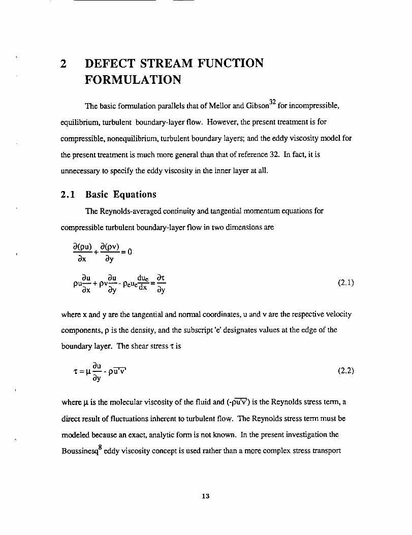
The Reynolds-averaged continuity and tangential momentum equations for
compressible turbulent boundary-layer flow in two dimensions are
O(pu)+ _(pv...._2)=03x 3y
_u _u du_PU_xx + pV_yy- peUe--a--_- = _Y
(2.1)
where x and y are the tangential and normal coordinates, u and v are the respective velocity
components, p is the density, and the subscript 'e' designates values at the edge of the
boundary layer. The shear stress x is
Ou'¢ = ix 7-- - ph-_ (2.2)
oy
where Ix is the molecular viscosity of the fluid and (-p-'d_) is the Reynolds stress term, a
direct result of fluctuations inherent to turbulent flow. The Reynolds stress term must be
modeled because an exact, analytic form is not known. In the present investigation the
Boussinesq 8 eddy viscosity concept is used rather than a more complex stress transport
13
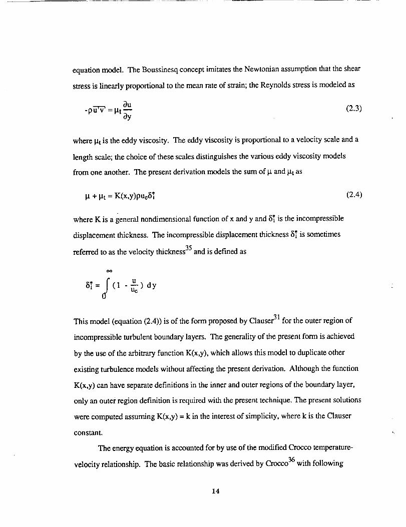
equationmodel. TheBoussinesqconceptimitatestheNewtonianassumptionthattheshear
stressis linearly proportional to the mean rate of strain; the Reynolds stress is modeled as
3u (2.3)-ph-7 = l.tt 3y
where l.tt is the eddy viscosity. The eddy viscosity is proportional to a velocity scale and a
length scale; the choice of these scales distinguishes the various eddy viscosity models
from one another. The present derivation models the sum of ix and P.t as
I.t + l.tt = K(x,y)pueS_ (2.4)
where K is a general nondimensional function of x and y and 8'_ is the incompressible
displacement thickness. The incompressible displacement thickness 8'_ is sometimes
referred to as the velocity thickness 35 and is defined as
j u5*= (1 -_) dy
This model (equation (2.4)) is of the form proposed by Clauser 31 for the outer region of
incompressible turbulent boundary layers. The generality of the present form is achieved
by the use of the arbitrary function K(x,y), which allows this model to duplicate other
existing turbulence models without affecting the present derivation. Although the function
K(x,y) can have separate definitions in the inner and outer regions of the boundary layer,
only an outer region definition is required with the present technique. The present solutions
were computed assuming K(x,y) = k in the interest of simplicity, where k is the Clauser
constant.
The energy equation is accounted for by use of the modified Crocco temperature-
velocity relationship. The basic relationship was derived by Crocco 36 with following
14

assumptions:steadyflow of aperfectgas,Prandtlnumber(Pr)of one,which impliesa
perfectbalanceof viscousdissipationandheatconduction,streamwisepressuregradientof
zero,andaconstantvalueof thespecificheatcoefficientCp.Thebasicrelationshipis
u2T-- w+
where Tw is the wall temperature and Taw is the adiabatic wall temperature. Baronti and
Libby 37 have made a detailed investigation of the accuracy of the Crocco relation for
adiabatic flows and state that they found deviations of less than plus or minus four percent
in the static temperature ratios obtained throughout the boundary layer• Gran, Lewis, and
Kubota 38 have compared this relation to nonadiabatic experimental cases and found no
significant deviation. White 22 shows a modification to this equation in which a recovery
factor is introduced as follows:r
T=Tw+(Taw-Tw) u ru 2
where r is the recovery factor and is defined as r=-Pr 1/3 for turbulent flow (r=Pr 1/2 for
• 22laminar flow). This equation has proven to be a very good approximauon" of the energy
equation even beyond the bounds of the strict assumptions.
Adiabatic wall conditions are assumed in the present study; the modified Crocco
temperature-velocity relationship for adiabatic walls is
Tw P=l+r =l+r M 2"T"= Pw
(2.5)
where _ is the ratio of specific heats (taken to be 1.4), a is the speed of sound, and M is the
Mach number• The Prandtl number is assumed to be 0.72 in this study. The simplicity
and effectiveness of this relationship avoids the use of the differential energy equation and
the corresponding need for temperature laws of the wall and wake.
15

In thistreatment,thedefectstreamfunctionof Clauser30'31is modifiedto account
for compressibility.Thedefectstreamfunctionf(_,rl(x,y)) of thisformulationisdefined
suchthat
U-U eb---_f= f'(_,rl)= ""7- (2.6)
u
where the transformed coordinates are
Y
fP--dyp== x and rl=7
The coordinate transformation incorporates a density weighting integral similar to that
originally proposed by Mager 39. This particular transformation of the normal coordinate
was chosen because it reduces to the form used by Clauser, and then Mellor and Gibson,
for incompressible flow. The shear-stress velocity u* is defined as
where Pw and Xw are the density and shear stress at the wall. The compressibility
transformation yields the density-weighted velocity thickness _,, which appears throughout
the derivation and is defined as
U8v = (1 -_) dy
The boundary layer defect thickness parameter A is defined as
16

OO Oo#0f u ue .A=- _dy=7 (1 -_)dy= "7
or
An* = ue_ v
Partial derivatives with respect to x and y are of the form
m= _._. _ and xan =Apo
2.2 Law of the Wall and Wake
It is assumed that a law of the wall and wake for velocity in the inner part of the
boundary layer is known. This law is of the form
U= g(y+,Me) + h(13,q,Me)
U(2.7)
where g is the law of the wall and h is the law of the wake. The inner variable y+ is
defined as
* Res* =y+ =u Y=_n
Vw
where o and _1 are defined as
¢o _ and Yl y_ a
and the Reynolds number based on the edge velocity, the incompressible displacement
thickness, and kinematic viscosity at the wall is defined as
ueST u*aRes* = _ = _ 0
Vw Vw
17

Thecompressiblepressuregradientparameter,whichreducesto Clauser'spressure
gradientparameterfor incompressibleflow, isdefinedas
= ,_'_ dx
where p is the pressure. A modified form of the parameter 13will be def'med later and
shown to be the compressible equilibrium parameter. For nonequilibrium flow, this new
parameter is a function of x and hence _; for equilibrium flow, this parameter is constant.
In the present lreatment, van Driest's 19 effective velocity (or generalized velocity)
approach, as simplified for adiabatic flows and modified by the recovery factor, is used for
the law of the wall:
g(y+'Me) = qr_2__l ) "u*"(aaw_sin{q r(_'-l'-''_) (_-aw) (lln y+ +B)}2 _: (2.8)
where aaw is the adiabatic wall speed of sound and _ and B are the law of the wall
constants. Van Driest's derivation parallels Prandtl's 40 derivation for incompressible flow.
The assumptions used are that the shear stress in the fluid is constant and approximately
equal to the shear stress at the wall and the mixing length is linearly proportional to the
distance from the wall. Van Driest incorporated a variable density into the derivation in the
form of the Crocco relationship. Again, equation (2.8) has been simplified for flows with
adiabatic wall conditions. Because the ratio (u*/aaw) is generally small, the law of the wall
is often used as
g(y+,Me) = lln y+ + B + O[(aU-_) 2]
Neither of these expressions is valid in the laminar sublayer.
18
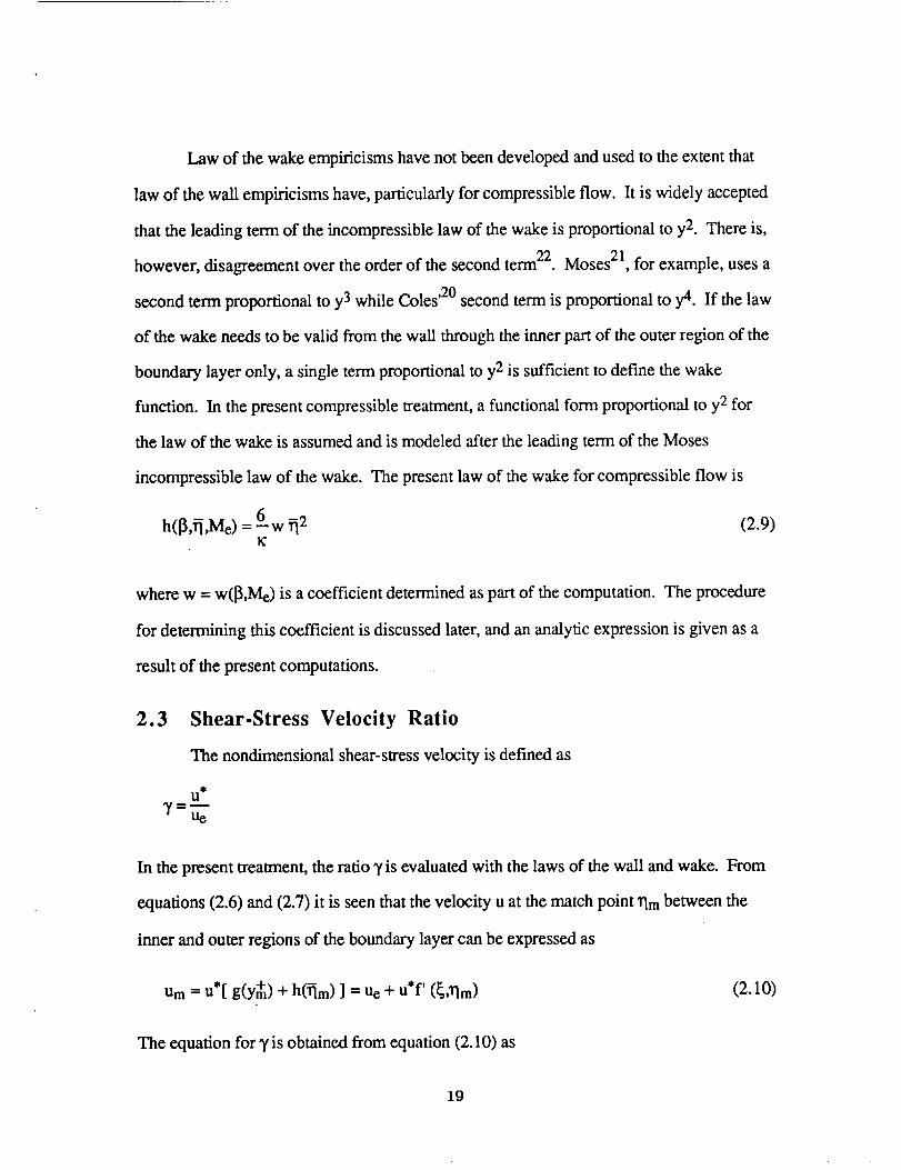
Law of thewakeempiricismshavenotbeendevelopedandusedto theextentthat
law of thewall empiricismshave,particularlyfor compressibleflow. It is widelyaccepted
thatthe leadingtermof the incompressiblelaw of thewakeis proportionalto y2. Thereis,
however,disagreementovertheorderof thesecondterm22. Moses21,for example,usesa
secondtermproportionalto y3while Coles'20secondtermis proportionalto y4. If thelaw
of thewakeneedsto bevalid from thewall throughtheinnerpartof theouterregionof the
boundarylayeronly, asingletermproportionalto y2is sufficientto definethewake
function. In thepresentcompressibletreatment,a functionalform proportionaltoy2for
the law of thewakeis assumedandis modeledaftertheleadingtermof theMoses
incompressiblelaw of thewake. Thepresentlaw of thewakefor compressibleflow is
h(]],_-l,Me)= 6 w _2 (2.9)!(
where w = w(13,Me) is a coefficient determined as part of the computation. The procedure
for determining this coefficient is discussed later, and an analytic expression is given as a
result of the present computations.
2.3 Shear-Stress Velocity Ratio
The nondimensional shear-stress velocity is defined as
U*
T=ue
In the present treatment, the ratio T is evaluated with the laws of the wall and wake. From
equations (2.6) and (2.7) it is seen that the velocity u at the match point rlm between the
inner and outer regions of the boundary layer can be expressed as
Um=u*[g(y+) + h(_lm) ] = Ue + u*f' (_,rlm) (2.10)
The equation for),is obtained from equation (2.10) as
19

1
7=[ gm + hm - f_ ] (2.11)
In the analysis that follows an expression for the gradient of y with respect to _ is needed.
Differentiation of the above expression yields
_'= -y2 [ gm + _m - _a ] (2.12)
where
The derivative of the law of the wall (equation (2.8)) with respect to _ is
= m_ O U* 2
tCy Ue A Vw(2.13)
Substitution of equation (2.13) into (2.12) yields
Ue_/= lC [ 1 +ue(__V__w) ]-t Pe A (hm - t'_a)
Ue Y (1 + T_..) ue A Vw pwl3 (1 + Y)
This term was neglected by Clauser 31 but was found to be important and included by
Mellor and Gibson 32 in their incompressible analysis. The present compressible analysis
will also require the following relationships:
Pe v Ue
_'..._.w= _tw Pw
Vw _w Pw
20
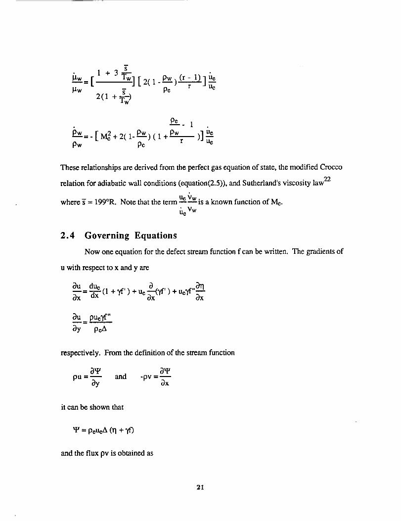
1+3 gg.__w=[ T-w'w][ 2( 1_ p_._w)(r- I) ] {le_tw Pe ?
2(1 +_
Pc_ 1
I_w=. [ M_ + 2( i.pw) (1 + pw )]Uepw Pe ""7--
These relationships are derived from the perfect gas equation of state, the modified Crocco
relation for adiabatic wall conditions (equation(2.5)), and Sutherland's viscosity law 22
where g = 199°R. Note that the term Ue Vw is a known function of Me.
Ue Vw
2.4 Governing Equations
Now one equation for the defect stream function f can be written. The gradients of
u with respect to x and y are
b u= due (1 0--4_bx "SZ" +_')+U_bx,,.')+u_Tf"_
bU pueTf"
by pea
respectively. From the def'mition of the stream function
bte btem .--n
pu= by and -pv bx
it can be shown that
W = peueA (rl + _')
and the flux pv is obtained as
21

(2.14)
In thedefectstreamfunctionformulation,thetangentialmomentumequation,equation
(2.1), is
--- __ ue A)COpe [K(P)2f,,], + Pe (2f' +Tf'2)-(1 + -- [(rl +Tf)f"
I_ Pw Pe Pw UeA
_: Ue{'w 2 ,fff,,)c 2 ,yf)f,, + (f, +T f, )4 (f' + Tf' - Tff")] + M_(TI +
(I +'Y) (1 +I-Y)UevwR: K
( Pe (-_- =-_)(f' +Tf' 2 - Tff" )
(1 + _.T)PwK
_Pe 1 [0f' Tf'0f' Tf,,0f]- TCw + -57-
(2.15)
where s is the nondimensional tangential coordinate def'med as
2.5 Boundary Conditions
There are two surface boundary conditions and one far-field boundary condition.
From equation (2.14) for the flux pv, the normal flow boundary condition at the surface,
v = 0 at rl = 0, is observed to correspond to
f(s,0) = 0
22

Thefar-field boundaryconditionisobtainedfrom thedefinitionof theboundary-layer
defectthicknessA:
A =- P _dy = -A _dll = A (f(s,0)- f..(s))
It follows that
f** (s)= -1 (2.16)
This boundary condition requires that u approach Ue as y approaches infmity. The final
boundary condition involves the shear stress at the wall. The shear-stress boundary
condition is
Xw = _u_ (i-t + I-tt) _
This boundary condition can be written as
2 2, ,,K(_,rl)p Ue 8i'Yf
pwU*2 pax
or
_x_ K(_,ll)(pP---22f''=leoP__Wpe(2.17)
This boundary condition replaces the usual no-slip boundary condition at the surface
(u(s,0)=0) and states simply that the shear stress must approach the wall shear stress as y
approaches zero.
It should be noted that these boundary conditions reduce to those used by Mellor
32and Gibson for incompressible flow.
23

2.6 First Integral of Governing Equation
It is always desired to reduce the governing equations to their simplest form
analytically before turning to numerical analysis. The advantage of such an analytic
integration is twofold: the order of the equation to be solved numerically can be reduced,
and boundary conditions can be absorbed and not imposed numerically. The defect stream
function governing equation has a first integral, and one boundary condition is absorbed
analytically. As will be seen, however, a limited advantage is gained for the full equation.
It is only upon making the zero-order approximation in the limit of vanishing shear-stress
velocity ratio that the full advantage is gained.
Equation (2.15) can be written as
[ OeK (2.)2f,,[_ Pw Pe
ueA) (1-$f')f+2Pef-(l+ {rlf'" } +pw --ZJ
Ue (1 +2)K
@) Pe [dhm dffia'_ (1-Tf')f
(1 + 2)Pw'"d'7-" ds /K
_(1-Yf')f(Me2+2{M2_UeVw }) Pe 1 _f
( 1 + 2) _ fie Vw Pw _ c)sK
__, 2
(1 +Y)K
UeA Pe 2({l+ueh.[(1 + .--_-) - M_ +---
+ Pe Yf, _)f],Pw 13 _s
2pe (dhm df_/1 Pe T3f'2+M_-2 ue_'w Pe-)+213pw_,d s - ds.,a +
/_eVw Pw Pwf_ as
Using the boundary condition given in equation (2.17), the above equation can be
Ue Aintegrated across the boundary layer to evaluate the quantity 1 + ----. This value is
Ue A
24

&uoa1+ -[(I+Y--) 1 pe{2 - . _ Ue_'w----= + "I_3} Me2 {1-yG}-
{le A _: Pw (1 +_-Y)Ue vw1¢
'Y Pe (dhm dd__)+Oe TdG)+ (1 2"1_3)][1-'_3(1-T)] "1
1
= 1 +m----_ •
(2_K} - 1)
(2.18)
where the defect shape factor G is defined as
It is necessary to incorporate a Mach number scaling effect into the coordinates in
order to determine the conditions for compressible equilibrium flow. The following
transformation allows for this effect:
s
a-f es aria_Pe _/ Pe
Applying this transformation and integrating across the boundary layer, the first integral of
the governing equation for arbitrary _ is
(1__,) _ss=0f 0_(O..p.)2Kf,,pe -[3(1 + 1-M_)(_f'm _ (1-_')f)(I+'_Y)
K
&K
• A
_(1-_' )f(M_ - ueVw-) + 213 Pe f - 1 +.T......_[ [3(1-_lm- M_ +Pe)(1_ T_)
(I+Y) _eVw Ow (1 +.Y.Y) Ow _¢K K
^
rl
1¢ _eVw Pw ' _ Pe ds
(2.20)
25

A A
rl rl^() r, 2
-pwO"_'e_..t[3"I-PW)(l-(1-r)-P--_-)[_f'OePe + _,Jf,2 d_l)]-Y_ss_f d_
(1+Y-ItT _ Pe.sK
where the prime denotes partial differentiation with respect to _1. The term (1 + 1) is
A °
defined in equation (2.18), and the parameter 71s defined as
Note that for the adiabatic wall conditions of this investigation, the density ratio (Pw/Pe) has
values between zero and one, which assures that _, is less than or equal to 7. Expressions
for the ratios o3 and (Pe/P) can also be written in defect stream function form:
8T I/f, 2 __/pwCo=_'= 1 + C. (1 + rN "_"e
P._e= l+r (_.M_[l'(_)2]=l-ef'[l+2N_e ]P
where
_=2Y_pP--_(1-_)po
For edge Mach numbers from incompressible to supersonic this parameter is small so that
the ratios (_ST/G) and (Pe/P) are approximately one. However, because E has the limiting
form
26

_Me
it is not small for large values of the edge Mach number. The term e is similar to Coles '41
parameter cfM_, which remains finite for large Mach numbers. The skin friction coefficient
cf is equal to (2Xw/poouo,2).
It is apparent that the analytic integration shown in equation (2.20) provides an
advantage over equation (2.15), the equation before integration. The governing equation,
which is now in the form of an integro-differential equation, has been reduced to second
order (leading derivative of f") and one boundary condition (equation (2.17)) has been
absorbed analytically. The integral terms in equation (2.20) are of higher order, and are
evaluated easily when solving this equation. The full advantage of the first integral
equation is seen in the next section where the zero-order approximation is made.
2.7 Zero-Order Approximation
As mentioned previously, the shear-stress velocity ratio ), is generally small. As a
result, the dependent variable of the defect stream function formulation f can be expanded
in terms of the shear-stress velocity ratio. Mellor and Gibson 32 used this expansion in their
incompressible analyses to obtain a zero-order, asymptotic form of the governing equations
with respect to the shear-stress velocity ratio. The expansion of f is
f = fo + Tfl + T2f2 + ....
Asymptotic forms are obtained for equations (2.18) and (2.20). For hypersonic flow,
these asymptotic forms are not the strict zero-order forms because the term 8 appears in
both o and (Pe/P) and is not negligible. The constrained zero-order forms of equations
(2.18) and (2.20) are
27

ueA 1+ 2Pe_M_)
pw
foIo_,= co I_h¢'(_+ (I+213)^ '- -
^
where the pressure gradient parameter 13is deemed as
(I.P__..w)Pe (1_ Pw{ l_r})]= P"e'-e13[1 " 2r
Pw Pe
(2.21)
Note that equation (2.21) is linear from incompressible to supersonic flow because co and
(Pe/P) are approximately one. An additional transformation is necessary to obtain a
governing equation which is linear in the hypersonic range. This transformation is
described in reference 42 and shown in Appendix A.
The full advantage of analytically integrating the governing equation is now
apparent. The terms in equation (2.20) are either simplified or eliminated when making the
zero-order approximation; the integral terms of equation (2.20) are considered to be small
and are neglected. The result is simply a second order differential equation and one
boundary condition has been absorbed analytically.
2.8 Equilibrium Flow Approximation
The equilibrium condition, as defined by Mellor and Gibson 32, occurs
mathematically when the profile of f, and hence u, depend only on the nondimensional
normal coordinate and not on the streamwise coordinate. These authors noted that the
streamwise partial derivatives are zero when the coefficients of the governing equation are
independent of the streamwise coordinate, and they showed that this condition can be met
exactly for the zero-order incompressible equation and approximately when higher order
terms are included. This same situation pertains for compressible flow. If K does not
28
depend on s, is constant, and both co and (Pe/P) are approximately one, the coefficients
• A
of equation (2.21) are independent of s and, since the boundary conditions are also
independent of_, the derivative on the left side of equation (2.21) is zero. The more
A
complicated coefficients of equation (2.20) depend weakly on s.
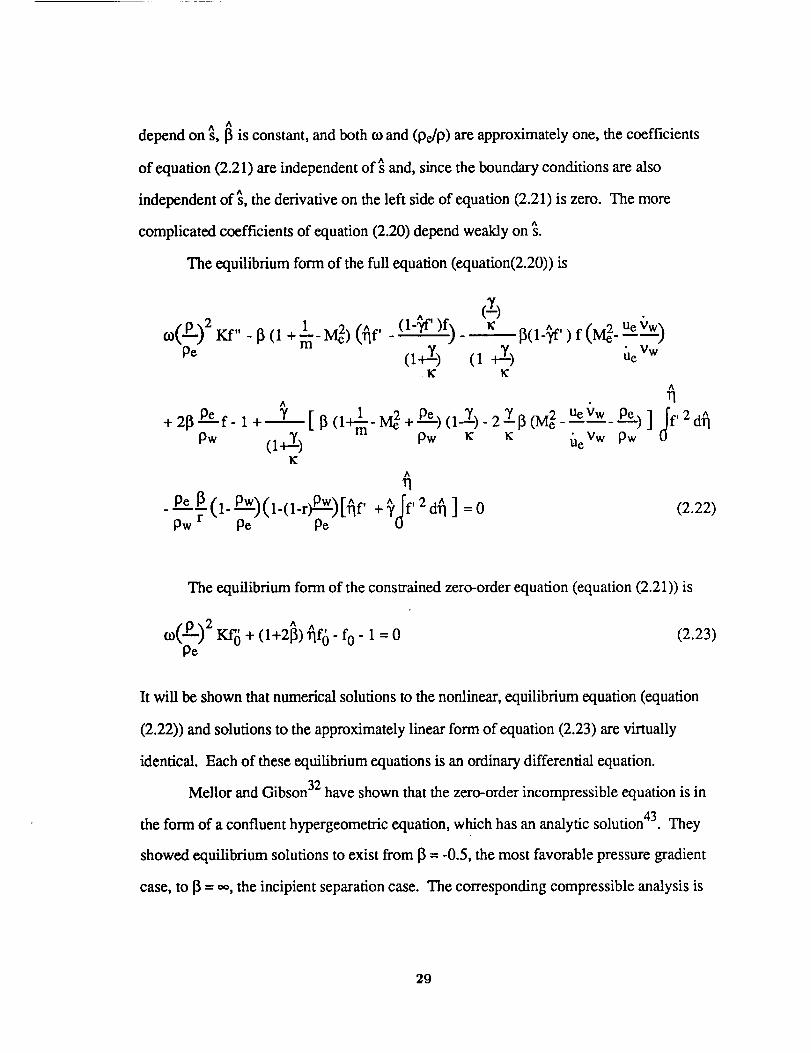
The equilibrium form of the full equation (equation(2.20)) is
1 (1-'_tf' _(l__/f, ) f (M_. Ue Vw)t0(P---)2 Kf '' -_(1 +_-M_) (_f' - )f)_ x:
Pe (1+ _'y) (1 -_-Y) Ue vwK K
A
+ 213 Pef. 1 + Y [ 13(l+-_lm - M_ + Pe) (1.Y.Y)_ 2--Y13 (M_
Pw (1._.Y) Pw ic _cK
A
n
Pw r Pe Pe
A
rl
Ue Vw Pe.) ] Jf, 2 d_ueVw Pw
(2.22)
The equilibrium form of the constrained zero-order equation (equation (2.21)) is
c0(P--_.-)2Kf'6 + (1+2_) ^ 'rlfd- f0- 1 =0 (2.23)Pe
It will be shown that numerical solutions to the nonlinear, equilibrium equation (equation
(2.22)) and solutions to the approximately linear form of equation (2.23) are virtually
identical. Each of these equilibrium equations is an ordinary differential equation.
Mellor and Gibson 32 have shown that the zero-order incompressible equation is in
the form of a confluent hypergeometric equation, which has an analytic solution 43. They
showed equilibrium solutions to exist from _ = -0.5, the most favorable pressure gradient
case, to 13= .0, the incipient separation case. The corresponding compressible analysis is
29
presented in reference 42, and the analytic solution for compressible flow is given in
Appendix A.
30
3 Inner Region Treatment
It is this treatment which most distinguishes the present method of solution from
previous methods. In effect, the treatment replaces the inner region numerical
computations with an empirical representation. The inner region generally encompasses the
inner-most twenty percent of the boundary layer and can extend beyond the logarithmic
region of the boundary layer. It can also be thought of as the region where an inner eddy-
viscosity model is used in the zero-equation eddy-viscosity approach. The need for an
eddy-viscosity model in this region is completely eliminated. The empirical representation
is in the form of the law of the wall and the law of the wake for velocity as defined in
equation (2.7) and the modified Crocco relation for the temperature as defined in equation
(2.5). The laws of the wall and wake need 0nly be valid in the inner region for the present
method; the Crocco relation is used across the entire boundary layer. The outer region of
the boundary layer is where the outer eddy-viscosity model pertains.
In general, there is one point, the "match point," where both the laws of the wall
and wake and the outer eddy-viscosity model are correct. The present treatment assures
that the derivatives of the defect stream function through f" are continuous at this point.
The term "match point" should not be construed to mean that the inner and outer solutions
are being matched in the formal sense. Actually, these solutions are being patched at one
point. As discussed in references 17 and 18, this procedure is completely analogous to
patching the inner and outer eddy viscosity models in the zero-equation modeling approach.
It should be noted that the inclusion of the law of the wake in the inner layer model
means that the match point is not confined to the logarithmic part of the boundary layer.
Several key points must be addressed when deriving and implementing this inner
region treatment. First of all, an equation relating the velocity, as represented by f', and its
integral, represented by f, through the inner region must be available to insure a continuous
solution across the match point. Secondly, an equation which allows the determination of
31
the match point as part of the computation must be determined. Finally, a procedure must
be developed which allows the implementation of the patching of the inner empirical and
outer numerical solutions in an efficient manner. These points will now be addressed.
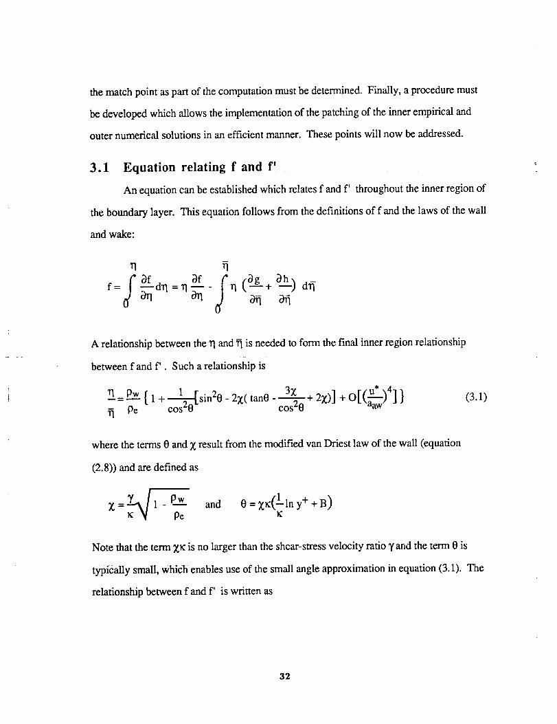
3.1 Equation relating f and f'
An equation can be established which relates f and f' throughout the inner region of
the boundary layer. This equation follows from the definitions of f and the laws of the wall
and wake:
jafan onaf f (a__g_.g+Oh)
f= ='-dtl = tl _- - TI -- dtl
A relationship between the 1] and tl is needed to form the final inner region relationship
between f and f'. Such a relationship is
{1 +----_-sin20 - 2)c(tan0- 3__ + 2)0] +O[(a_w)4]}
rl Pe cos20 t cos20
(3.1)
where the terms 0 and )Cresult from the modified van Driest law of the wall (equation
(2.8)) and are defined as
=Y_[ 1 - p..._.w and
Pe
0 = )Clc(1 In y+ + B)K
Note that the term Z_c is no larger than the shcar-stress velocity ratio Y arid the term 0 is
typically small, which enables use of the small angle approximation in equation (3.1). The
relationship between f and f' is written as
32

cosO{cos20 - 3)_sinO cosO+ 12X 2 - 7_2cos20]. f _h'_ cos_O 2zsinO cosO q-;Vp:'h_ "_)- --d_
The lowest order approximate relationship between f and f' is written as
f = rl(_'- 1) - f rl°ah dfl + O[(a_w )2]!¢ o_
(3.2)
This equation pertains throughout the inner region, where the empirical law of the wall and
wake is valid. Note that because h is proportional to _12, the integral term is proportional to
_3; the integral term is small throughout the inner region because _lm is small. The use of
this equation at the match point insures the continuity of f and f'. The match point is
positioned so that the derivative f" is continuous. The transformation given in equation
(2.19) is easily applied to the equations of this section.
3.2 Match Point Location
The match point location is determined using the equilibrium form of equation
(2.20), which is the first integral of the tangential momentum equation as given in equation
(2.22), and equations (2.7) and (2.8) for the law of the wall and wake, which are used to
evaluate the f" term in equation (2.20). The equilibrium flow assumption can be used
because the derivatives with respect to ^ "s m equation (2.20) are small in the inner region
where the match point is located. Equation (3.2) is used to relate f and f'. Equation (2.22)
is evaluated at the match point and, with some manipulation, the constrained zero-order
form of the governing equation is
33

Kp0_{ l"_+(c)h)m} +(l+2_)_lm(_fAf) -fm-l=0Pw icl'lm _ m
(3.3)
Usingthetransformationgivenin equation(2.19)andequation(3.1),thelowestorder. A
relauon between rl and _ is
Because the law of the wake in equation (2.9) is of order _12 near the wall, the
integral term in equation (3.2) is of order _3 and can be neglected as _lm is small. If
equation (3.2) is substituted into equation (3.3), the equation for the match point location is
K p_m..m= 0AV'I2- Vqm +--co (3.4)_: Pw
where the constrained zero-order form of the term A is
1 _ _+ 2Ao(_f'_ / 12w K po).__..A = (pw)3/2pe {TN _'w P('_ "1m1 +--lc Pw
(3.5)
It is in equation (3.4) that the law of the wake plays its most significant role in the analysis
and, from equation (3.5), it is the leading coefficient of the law of the wake which is truly
significant. The solution for _qm is easily determined from equation (3.4) as
1-_I-4AKo,) Pm_-lm = Pw2A (3.6)
3.3 Implementation of Inner Region Treatment
There are several methods with which to implement this inner region treatment.
The essential feature is that the inner region formulation properly interact with the
numerically computed outer region solution. As discussed earlier, the formulation is such
34

that f, f', and f" are continuous at the interface between the two regions. In primitive
variable terminology, this means that the integral of the velocity profde, the velocity u, and
the velocity gradient _u/by are continuous across the match point. In effect, the inner
region formulation provides boundary conditions for the outer numerical solution. This is
the same concept that has been used in other wall function methods. Again, the main
differences of the present method are the increased region of the boundary layer that is
modeled empirically and the fact that the size of this region is not predetermined by the
researcher (ie. previous methods limit the use of empirical expressions to a predetermined
distance from the wall) but is determined as part of the solution process.
Once the match point is determined, empirical expressions are evaluated at this point
so that the properties of the flow are determined and used as boundary conditions for the
numerical computation of the outer region. These new boundary conditions replace the
traditional no-slip at the wall boundary conditions normally enforced at the wall for viscous
flows. The region of the boundary layer requiring numerical computation on a highly
clustered grid is significantly reduced. This is true for previous wall function methods and
was, in fact, the main incentive behind the development of these methods. As mentioned
before, the present treatment increases the savings.
At a given streamwise location, the present treatment yields a single, physically
accurate match point location; this location, however, is variable in the streamwise
direction. Problems with the implementation of the new boundary conditions arise because
the grid is typically established prior to the numerical computations; it would be fortuitous
if the variable location of the match point would always, or ever for that matter, fall on an
existing grid point. Computationally, there are several options as to the point of application
of the empirically determined, match point boundary conditions.
The obvious In'st option is to apply an adaptive grid technique that forces the grid
point nearest the wall to coincide with the match point at each streamwise location; the first
35

grid point off of the wall adjusts itself with each iteration, or time step, during the
computation such that it is always located at the current match point. The match point
boundary conditions are enforced at the f'trst grid point. This approach is very complex for
the general case of nonequilibrium flows, but is relatively simple for equilibrium flows.
This is the primary approach used in the present investigation when computing equilibrium
flows (both incompressible and compressible); the details of this technique as applied here
for equilibrium flows are given later.
An approach must be developed that relates the match point to a general, fixed grid.
Several options present themselves. Since the inner region of the boundary layer is thin
relative to the boundary layer thickness, it should be admissible as a first approximation to
impose the match point boundary conditions at the geometric surface. This is comparable
to translating the point of application of boundary conditions in thin airfoil theory to the
airfoil chordline. A more accurate approximation is to apply the match point boundary
conditions at the grid point closest to the match point. Flowfield information at the grid
points between the match point and the surface is supplied by the law of the wall and wake.
Another possibility is the definition of a new transformed normal coordinate that is
defined such that the match point is located at a constant value of the new coordinate for all
streamwise locations. Such an approach requires the definition of a scaling function used
in the transformation of the normal coordinate. The scaling function is dependent on the
streamwise location and varies from flowfield to flowfield. Melnik 44 and Walker, Ece, and
Werle 12 have developed methods incorporating this approach.
The notion of applying surface slip velocity boundary conditions is reminiscent of
Clauser's 31 analysis of the outer region of turbulent boundary layers and comparison to
laminar boundary layers with slip velocities. Note the slip velocity corresponding to the
outer region shown in figure 2d. It would be desirable to use information determined from
the inner region treatment and the matching process to define surface boundary conditions
36

which enable the proper numerical computation of the outer region of the boundary layer.
In effect, the outer region is assumed to extend all the way down to the wall so that only an
outer eddy-viscosity model is required. The shear stress at the wall associated with the
outer eddy-viscosity model is forced to be equal to the physically accurate wall shear stress.
As a result, the numerical computations from the wall to the match point yield nonphysical
information. However, the numerical solution becomes physically accurate upon reaching
the match point, thus providing the proper description of the outer region. The condition
specified in this approach is on the velocity gradient at the wall, which implies a condition
on the shear stress at the wall. In words, the numerically computed wall shear stress must
be equal to the physically accurate wall shear stress which is determined from the empirical
inner region and matching treatments. Mathematically, the boundary condition on the
velocity gradient enforced at the wall is
"'- z- I.t+l.tt - KpsueS_(3.7)
and is written in defect stream function variables as
[=a_.( af .,i1 pw (pe) 2 6T
This equation is a direct result of the definition of the shear stress (equation(2.2)) using the
eddy-viscosity concept (equation(2.3)). The arbitrary function K is chosen in the form of
an outer region model, such as K=k where k is the Clauser constant. This outer solution
includes a nonzero surface slip velocity and the associated surface density Ps.
Conditions on the velocity gradient at the wall ha_,e been used prior to this
investigation by other researchers. The condition used by Gorski et a145 is common among
wall function approaches. The condition is of the form
37

and is simply the derivative of the common logarithmic law of the wall. This condition
does not enforce the outer region model at the wall, but rather provides the compatibility
between the velocity, as determined from the law of the wall, and its normal derivative in
the near wall region. Melnik 44, on the other hand, has developed a condition for
incompressible flow that is also in the tradition of Clauser. His condition, which was
developed independently from the present investigation, is essentially the same condition as
the incompressible form of the present boundary condition.
It is felt that the implementation of the inner region treatment will be best handled in
the general, nonequilibrium case by use of the slip-velocity approach just described. This
approach is used in the primitive variable applications of this investigation. It has also been
successfully implemented into the equilibrium boundary layer solution procedure using
defect stream function variables.
38

4 Results and Discussion
This chapter traces the development of the present method in chronological order.
The initial phase of the investigation involved the derivation of the nonequilibrium defect
stream function formulation for incompressible flows. The formulation reduces to that of
Mellor and Gibson 32 for equilibrium flow. The primary accomplishment of the
incompressible studies was, however, the development and implementation of the
technique used to match the empirical inner region solutions with numerically computed
outer region solutions. Another new feature was the use of a law of the wake in addition to
the law of the wall. An existing law of the wake was used in this part of the investigation.
The primary phase of the investigation was the development of the nonequilibrium,
compressible defect stream function formulation and the corresponding compressible inner
region treatment in conjunction with the matching of the inner and outer region solutions.
The compressible formulation was designed to reduce to the incompressible form of the
initial work. A method for determining the coefficients of a postulated compressible law of
the wake was also developed. This resulted in an analytic equation for the compressible
law of the wake valid from the wall through the inner part of the outer region.
The final phase consisted of the application of the present techniques in primitive
variable form. The method was incorporated into an existing two-dimensional Navier-
Stokes code and tested for several cases of compressible flow over a flat plate.
4.1 Incompressible Flow
Solutions for incompressible, equilibrium boundary layers have been computed
with the asymptotic, or zero-order, and full-equation forms of the present method. As
discussed earlier, the zero-order form is taken in the limit of vanishing shear-stress velocity
ratio. All solutions of this section were computed using the incompressible law of the
wake of Moses 21 which is one of the widely accepted incompressible laws along with that
39
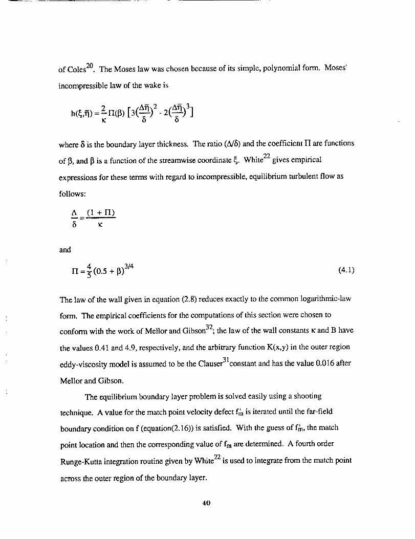
of Coles 20. The Moses law was chosen because of its simple, polynomial form.
incompressible law of the wake is
O Oh(_,rl) =2I-I(13) [3 - 2 ]K
Moses'
where 8 is the boundary layer thickness. The ratio (A/8) and the coefficient II are functions
of [3, and [3 is a function of the streamwise coordinate _,. White 22 gives empirical
expressions for these terms with regard to incompressible, equilibrium turbulent flow as
follows:
A (1 + FI)
5 K:
and
n = + [3)3/4 (4.1)
The law of the wall given in equation (2.8) reduces exactly to the common logarithmic-law
form. The empirical coefficients for the computations of this section were chosen to
conform with the work of Mellor and Gibson32; the law of the wall constants !¢ and B have
the values 0.41 and 4.9, respectively, and the arbitrary function K(x,y) in the outer region
eddy-viscosity model is assumed to be the Clauser31constant and has the value 0.016 after
Mellor and Gibson.
The equilibrium boundary layer problem is solved easily using a shooting
technique. A value for the match point velocity defect f_n is iterated until the far-field
boundary condition on f (equation(2.16)) is satisfied. With the guess of f_a, the match
point location and then the corresponding value of fm are determined. A fourth order
Runge-Kutta integration routine given by White 22 is used to integrate from the match point
across the outer region of the boundary layer.
40

The present solutions are compared with the full-equation solutions of Mellor and
Gibson 32. All of these results are for a Reynolds number based on the edge velocity and
displacement thickness (Res*) of 105. The comparison shown in figure 3 includes the
zero-order closed form solution for the most favorable pressure gradient, 13=-0.5. This
solution is shown in Appendix B. The present zero-order numerical solution is seen to be
in complete agreement with the closed form solution and in close agreement with Mellor
and Gibson's full-equation solution. The zero-order solutions provide an indication of the
accuracy of the numerical scheme; the numerical solutions give an early indication of the
accuracy of the zero-order equations.
It should be noted in figure 3 that the present method has resolved a turbulent
boundary layer with only eleven grid points across the boundary layer. It is fair to question
the accuracy of a solution with so few grid points. Figure 4 compares various grids for a
typical value of 13(13= 2) and shows that the eleven point grid solution is in agreement with
the 51 and 101 point solutions. Only the six point solution deviates noticeably from the
fine grid solutions, and this deviation is negligible. On the basis of these observations, the
present solutions were computed with eleven uniformly spaced grid points. The first grid
point is always at the match (patch) point, and the edge value of the normal coordinate is
fixed. This is the adaptive grid approach mentioned in section 3.3. The normal coordinate
reduces to rl for incompressible flow and is plotted as such. During the iteration of the
velocity defect f_, the first grid point Vim shifts with f_ according to equation (3.6). The
uniform grid is recomputed for each value of f_. This grid procedure was used for
convenience rather than necessity as the grid points other than the first could have been
fixed. By eliminating the inner region computations, a grid-point savings on the order of
fifty percent was realized as was the case in references 12, 13, 17, and 18.
Equilibrium velocity defect profiles are presented in figure 5 for several small-[_
cases (13 < 1); and in figure 6, results are presented for large-_ cases (13 > 1). The
41
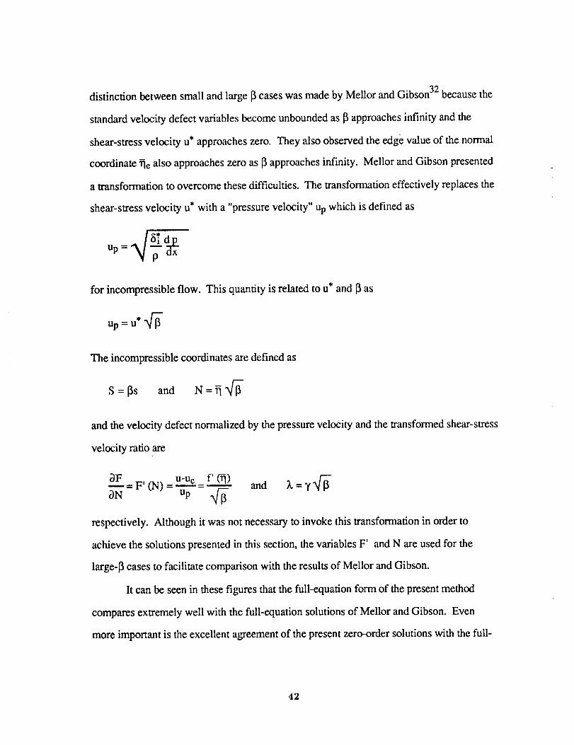
distinctionbetweensmallandlarge13caseswasmadebyMeUorandGibson32becausethe
standardvelocitydefectvariablesbecomeunboundedas13approachesinfinity andthe
shear-stressvelocity u* approacheszero. Theyalsoobservedtheedgevalueof thenormal
coordinate_ealsoapproacheszeroas13approachesinf'mity. Mellor andGibsonpresented
atransformationto overcomethesedifficulties. Thetransformationeffectivelyreplacesthe
shear-stressvelocity u* with a "pressurevelocity" Upwhich is definedas
Up = _ dx
for incompressible flow.
Up = U* "@"
This quantity is related to u* and 13as
The incompressible coordinates are defined as
S = 13s and N = _
and the velocity defect normalized by the pressure velocity and the transformed shear-stress
velocity ratio are
3F=F'(N) U-Ue f'(_) and X=7"@'-
ON Up @-
respectively. Although it was not necessary to invoke this transformation in order to
achieve the solutions presented in this section, the variables F' and N are used for the
large-13 cases to facilitate comparison with the results of Mellor and Gibson.
It can be seen in these figures that the full-equation form of the present method
compares extremely well with the full-equation solutions of Mellor and Gibson. Even
more important is the excellent agreement of the present zero-order solutions with the full-
42

equation solutions. The relative simplicity of the zero-order approach and its excellent
results makes it a desirable alternative to the full-equation approach.
The differences seen in the inner region are caused by the differences between
Mellor and Gibson's inner region eddy-viscosity model and the present combination of the
law of the wall and law of the wake. Mellor and Gibson's solutions approach the law of
the wall in the limit as _qgoes to zero. As will be seen later, Mellor and Gibson's approach
allows a large deviation from the law of the wall and wake in the inner region. This effect
becomes more noticeable with increasingly strong adverse pressure gradients (increasing
13).
The 13= 10 case shown in figure 6 was computed with the Clauser constant
k = 0.0154935 rather than k = 0.016. As demonstrated in'figure 7 for the zero-order
approach, a match point does not exist for 13= 10 with k = 0.016 because the far-field
boundary condition F** ----I cannot be satisfied. This failure to obtain a solution indicates
the problem is overspecified. Figure 7 shows that the value k = 0.0154935 yields a single
value of F_ that satisfies the far-field boundary condition for 13= 10. The maximum value
of 13for which a solution exists for k = 0.016 is approximately 8.6. For values of 13less
than 8.6, there are two values of fth which allow the far-field boundary condition to be
satisfied. The physically correct value is the smaller of the two.
The problem of overspecification is alleviated by allowing the law of the wake to be
computed as part of the solution, as discussed in section 4.2, rather than relying on a fixed
law of the wake as done when computing the solutions shown in this section. The
flexibility of computing the law of the wake allows solutions to be computed without
altering the Clauser constant as was done for the 13= !0 case shown in figure 4.
Results for the shear-stress velocity ratio "r from the present solutions are compared
with the results of Menor and Gibson in figure 8. The two sets of results are in close
agreement but are not identical.
43

The present method for evaluating Y differs substantially from that of Mellor and
Gibson 32, Walker et a112, and others in that the value of T is obtained from a patching of
the inner and outer solu .tions at a particular point in the present method whereas a matching
of _e outer limit of the inner solution with the inner limit of the outer solution is used in the
other methods. These methods are not strictly asymptotic in that the inner and outer eddy-
viscosity models are patched at a point analogous to the patch point used in the present
method. The equation Mellor and Gibson used to evaluate Y is very similar to equation
(2.11), the equation used in the present method. The difference is one of application;
equation (2.11) is evaluated at a point a finite distance from the surface in the present
method, while the equation used by Mellor and Gibson is evaluated as close to the surface
as possible (the inner limit of the outer solution). As a result, the values of T obtained by
Mellor and Gibson are consistently smaller than those obtained by the present method.
However, larger values of T can be obtained from the results of Mellor and Gibson by
evaluating their equation at the point where the eddy viscosities are patched.
The inner region velocity profiles of the present method differ from those of Mellor
and Gibson. The differences increase with an increasingly strong adverse pressure
gradient (increasing 13)and are best displayed using inner variable coordinates. Figure 9a
shows the _ = 4 case. It is clear in this figure that, although the inner solutions are
identical near the wall, Mellor and Gibson's solution deviates from the logarithmic behavior
at least an order of magnitude (in y+ units) closer to the wall than in the present method.
This shows the difference between applying an eddy-viscosity model that approaches the
logarithmic form when approaching the wall and enforcing the logarithmic behavior
throughout the inner region. In view of this difference, a comparison with experimental
data seems appropriate. Figure 9b compares the present solution with experimental data
taken from reference 46 for Clauser's 30 second equilibrium flow. The data shown in
figure 9b correspond to profile 2305 in reference 46. For this profile, 13= 7.531 and
44

Re_. = 30692.5. Figure 9b shows excellent agreement between the experimental data the
present solution. Given the relatively large value of 13,one would expect less agreement,
especially in the logarithmic region, between a Mellor and Gibson solution and experiment.
The present solution and experiment were also in close agreement for _, where a 0.87
percent difference was found. Present solutions were computed and compared with
experimental data from reference 46 for many values of [3 and good agreement was
generally observed. Table 1 shows several comparisons of the experimentally and
numerically determined shear-stress velocity ratios where the numerical solutions were
computed with the zero-order formulation. The analytic solution from the method of
reference 42 (see Appendix A) is also shown.
Another feature of the present method can be observed quite well in figure 9b.
Notice that the match point of the present solution is well beyond the logarithmic region.
This result demonstrates the advantage gained when including the law of the wake in the
present formulation. For all present solutions, the law of the wake allows the match point
to move beyond the logarithmic region thus extending the usefulness of the analytic inner
region treatment and further reducing the region which must be resolved numerically. As
one would expect, the influence of the law of the wake increased as 13increased.
4.2 Compressible Flow
Solutions for compressible, equilibrium boundary layers have been computed with
the constrained zero-order and full-equation forms of the present method. The full-
equation solutions, however, were generated with the equations of the matching procedure
truncated to second-order. As discussed earlier, the constrained zero-order form is not the
strict asymptotic form taken in the limit of vanishing _' as the term E, which is of order'_Vle,
is not always a small parameter and thus remains in the formulation. The significance of
the term E increases with increasing Me and has been included in all of the present
computations for compressible flow. The term, however, is practically negligible until
45

reaching the high supersonic and hypersonic flow regimes. To fulfill the goal of
determining a compressible law of the wake, solutions were computed with an iterative
curve fit technique supplying the coefficient w of the postulated law of the wake given in
equation (2.9). An analytic expression for the coefficient w is determined from these
results.
The compressible equilibrium boundary-layer problem is solved using a shooting
technique in the same fashion as described for incompressible flow. The primary
difference is the determination of the law of the wake as part of the computational
procedure. The specific procedure for determining the coefficient w is discussed later,
suffice it to say that a new value of the coefficient w is determined with each iteration of frh.
The empirical parameters _cand B for the law of the wall and the outer region eddy-
viscosity parameter k retain their values from the incompressible flow cases; they are 0.41,
4.9, and 0.016, respectively. Note that the additional empiricism of the Crocco
relationship is also incorporated in the compressible flow computations.
Both the constrained zero-order and full-equation solutions have been computed^
over Me, _, and Res* ranges. The solutions shown were computed with 32 uniformly
spaced grid points across the outer region (the fhst point being the match point) in order to
facilitate the law of the wake curve fit procedure. Fewer points could have been used with
the same success if the points had been nonuniformly spaced and clustered near the match
point. Significantly fewer points were needed when the analytic law of the wake was used
(ie once the compressible law of the wake was determined and the curve fit procedure no
longer needed). The inner region solutions shown in the following figures were
determined analytically from the laws of the wall and wake and the Crocco relationship.
Figure 10 compares velocity defect profiles for the constrained zero-order and full-
A
equation formulations over a Mach number range for Res* = 104 and [3 = 0 (the flat-plate
case). It can be seen that the agreement between the formulations is extremely good. Table
46

2ashowstheshear-stressvelocityratioy computationsto bein agreementon theorder of
one percent across the Me range. The percent error of the constrained zero-order
formulation for the prediction of y, as compared to the full-equation formulation prediction,
increases as the edge Mach number decreases, but we have previously seen that the
predictions show excellent agreement for incompressible flow.
Figure 11 shows the comparison over a Reynolds number (Res*) range for Me = 3A
and 13= 0. Again, the velocity defect profiles are nearly identical and, as shown in Table
2b, the shear-stress velocity ratios as computed by the constrained zero-order formulation
show an error on the order of one percent. As the Reynolds number decreases, the percent
error of the constrained zero-order prediction of y increases.
A
Figure 12 shows the comparison for several 13values for Me = 3 and Re_, = 104.A
The 13= 1 case represents a relatively strong adverse pressure gradient case for supersonic
A
flow. The velocity defect agreement for the _ =I case, although not as good as for the flat
plate case, is still quite good. Table 2c shows the comparison of the shear-stress velocity
ratios computed by the two formulations. The percent error of the constrained zero-order
formulation increases with increasingly strong adverse pressure gradient. Although the
error seen here is larger than for variations of Me and Re_,, the error over this practicalA
range of 13's remains below five percent.
The reduced complexity of the constrained zero-order formulation and the excellent
agreement of the results above justify it as an excellent approximation and alternative to the
full-equation formulation. All subsequent solutions shown in this section are based on the
constrained zero-order formulation.
The determination of the law of the wake coefficient w is an important part of the
present solution procedure. The assumed, or postulated, functional form of the law of the
wake is shown in equation (2.9), where w is the unknown coefficient that is determined by
a least squares curve fit during each iteration of f&. Recall that for the present treatment the
47

law of thewakeneedonly bevalid in the innermostpartof theouterregion;thecurvefit to
determinew focuseson thisregionof theboundarylayer. In effect,avaluefor thelaw of
thewakehis determinedat eachpoint in theouterregionas
1 (4.2)
where g is the law of the wall, _, is the current value of the shear-stress velocity ratio, and
f' is determined from the numerical solution. A least squares curve fit of the values of h is
made with the value of the coefficient w as a result. A standard least squares correlation
factor was used to judge the accuracy of the fit. The number of points used for the curve fit
varied from case to case in order to maintain approximately the same correlation factor; that
is, approximately the same level of accuracy with regard to the fit was maintained from case
to case. Note that this procedure can be used for any general postulated law of the wake
with any number of unknown coefficients. More complex laws of the wake which could
be valid over more of the outer region of the boundary layer can be determined.
Figure 13 compares the resulting analytic law of the wake as defined by equation
(2.9) and the determined value of the coefficient w with the numerically computed values of
the law of the wake as determined by equation (4.2) for several Mach numbers. TheA
profiles shown are for Re_5* = 104 and _ = 0. It can be seen that the number of points
accurately fit by the postulated law of the wake decreases as the Mach number increases;
the fit is always accurate near the match point. From this figure, as well as other solutions
not presented, it appears that the y2 dominance of the law of the wake in the inner region
begins to diminish as Me approaches 4.
It can be seen in figure 13 that the law of the wake coefficient w is a function of Me
A
in addition to being dependent on [3. Figure 14a shows the variations of w as a function of
A A
Me and 13for Re_* = 104. It is seen that w increases significantly as 13increases, especially
48

at smallvaluesof Me. As theMachnumberapproaches4, w becomesarelativelysmall^
number for all 13,and the strong dependence of h on _i2 in the inner part of the boundary
diminishes. Figure 14b shows the variations of the coefficient w as a function of Me and
A
Res* for I3 = 0; the coefficient w is a weak function of Re_,.
An analytic model for the law of the wake coefficient based on the above solutions
can be written as
A
w(Me,_) = w(0,13) _Pe
A
where w(0,13) is the law of the wake coefficient for incompressible flow and the exponent
A
_ is a function of 13only. An equation for the coefficient w in incompressible flow follows
from section 4.1 as
w(0,13)= n = nK
(4.3)
where the coefficient I-I is a function of 13. White's 22 equation for rI, as given in equation
(4.1), can be used. Values of equation (4.3) based on equation (4.1) are shown in figure
14a in comparison to the values determined by the curve fit procedure. The present zero-
order solutions have been used to determine a new expression for 1-I. The equation is
rl = o1(0.5 + 13)a2 (4.4)
where a 1 and o 2 are functions of 13,rather than constants as in equation (4.1), and are
defined as
4 40.5+13°1 = ]" + 250 and 1 2 1 13)3/8]0 2 =_-+ _-exp[- _. (0.5 +
49

Figure 15a compares equations (4.1) and (4.4) with values of I'l deduced from the
numerically determined values of the coefficient w. Figure 15b compares the
corresponding values of the coefficient w. Equation (4.4) is seen to be an excellent
approximation to the numerical data throughout the range of 13. White never intended
equation (4.1) to be used for high 13cases, so the improvement in this range is not
unexpected. The agreement between equations (4.1) and (4.4) is much better in the low [3
range, but the new expression does fit the numerical data better. The equation for cz was
determined from the solutions shown in figure 14a and is written as
Ot(_) = 2 _ exp[_ 5_2_ + 1 ] (4.5)
The resulting curve is shown in figure 16.
As mentioned previously, significant grid reduction can be realized when using the
analytic law of the wake. Figure 17 shows this grid reduction when the analytic equation is
used rather than the curve fit procedure. The solutions shown for the case where Me = 3,
A
13= 0, and Res* = 104 are virtually identical with only the seven point grid solution
deviating ever so slightly. The computed values of y were also essentially identical as the
difference between the 32-point and the 7-point solutions was less than a quarter of one
percent.A
Figure 18 presents a series of constrained zero-order solutions over a 13range from
-0.3 to 2 for Res* = 104 and Me = 3. Profiles of the velocity defect, velocity ratio, and the
density ratio are given. Since it is unnecessary to evaluate the inner region solution in order
to compute the outer region solution, only the outer region results are shown. Figure 19
presents a series of fiat plate solutions for a Mach number range from 0 to 4 and for
Refi. = 104. Figures 18 and 19 are presented to document the effect of parameter variations
on the profiles. It is interesting to observe that Me variations have a minimal effect on the
velocity defect profiles. The velocity defect profiles for variations of Res* with fixed Me
50

A
and I_, although not presented here, were virtually identical. The fact that the velocity
defect prof'des are relatively insensitive to variations of Me and Res* supports the definition
A A
of 13as the compressible equilibrium flow parameter. The parameter 13effectively
designates the various families of similar solutions for compressible equilibrium flow, at
least under adiabatic wall conditions, in the manner shown by Clauser with his parameter 13
A
for incompressible flow. Note that the present parameter 13reduces to Clauser's 13for
incompressible flow.A
Figure 20a shows the effect of Me and 13on the shear-stress velocity ratio for
Res* -- 104. It is observed that y increases with increasing Me while decreasing with
A
increasing 13(increasingly strong adverse pressure gradient). For any combination of Me
A
and 13,y increases as the Reynolds number decreases. Figure 20b demonstrates this trend
for flat plate flow. The trend was documented in reference 32 for incompressible flow.A
Figure 21 shows the effect of Me, 13,and Re,i* on the compressibility parameter to.
Recall that this parameter is the ratio of the velocity thickness to the density-weighted
velocity thickness and appears throughout the present formulation. Figure 21a shows the
Mach number and pressure gradient effects on to for Res* = 104. By definition, to remains
one for all incompressible flows. It is observed that to increases with increasing Me as well
A
as with increasing 13. The effect of the pressure gradient is magnified with increasing Me.A
Figure 21b shows the effect of Res* on to for Me = 3 and 13= 0. It is observed that to
decreases with increasing Reynolds number. The curves of figure 21a would shift
upwards for Res* less than 104 and downwards for Res* greater than 104 with the
exception of the incompressible flow curve which remains fixed.
Comparisons of the constrained zero-order solutions with experimental data
compiled by Fernholz and Finley 47 have also been made. Figure 22 shows the profile
comparisons for two flat plate cases; each numerical solution was computed with 32 grid
points across the outer region and the curve fit procedure was used to determine the law of
51

thewakecoefficient.Theagreementof thevelocitydefectandvelocityratioprofilesis
good,while thedensityratioprofilesarein reasonableagreement.Theuseof theCrocco
relationshipfor thedensityratiomagnifiesthevelocitydifferences,especiallyneartheedge
of theboundarylayer. Themodificationof theoutereddy-viscositymodelby includingthe
intermittencyfactorwouldimprovethecomparisonsbecausethegradientof f' would
increaseastheboundarylayeredgeis approached.An intermittencyfactorcouldbe
incorporatedinto theformulationeasilyby allowingthearbitraryfunctionK in equation
(2.4) to bevariableratherthanusingtheClauserconstantk.
Table3comparesthecomputedandexperimentalshear-stressvelocityratios. The
computedsolutionsarefrom theconstrainedzero-orderformulationandtheexperimental
valuesarebasedon thevaluesof skinfriction asmeasuredby aforcebalance.Theanalytic
solutionsshownweredeterminedwith themethodof reference42. Theagreementfor the
flat platecasesisexcellent; theexperimentalandcomputedvaluesdiffer by nomorethan
twopercent.The5801seriesof experimentaldatarepresentsanonequilibriumflow in
whichdatawastakenin bothfavorableandadversepressuregradients.Theagreement
shownfor thisseriesis not asgoodasseenwith theflat platecases.However,the largest
differenceoccurswith thelargerof thetwo adversepressuregradientcasesandthe
differenceapproximately6.5percent.Theeditorsof reference47castsomedoubton the
accuracyof theexperimentalvaluesdueto alackof upstreamhistoryinformationand
unknownconditionsat theedgeof theboundarylayer. Thevalueof theshear-stress
velocityratio shoulddecreasebetweenprofiles5801/0501and5801/0801asMedecreases,^
13increases, and Res* increases; these trends, as observed in the present investigation,
indicate a decrease in ), that apparently was not observed experimentally.
4.3 Primitive Variable Application
The ultimate objective of the present investigation is implementation of the present
concepts into existing three-dimensional, Navier-Stokes methods. It should be at this level
52

thatthegreatestrewardswith regardtocomputationalefficiencyandaccuracywill be
realized.Coarsegridsareoftenusednearthewall in theinterestof computational
efficiency;theresultis a lossof accuracy.Accuratenumericalcomputationsnearthewall
requireafine grid,whichresultsin a lossof computationalefficiency. Thenumerical
computationsnearthewall canbereplacedbyanempiricaltreatmentthatdoesnotrelyona
fine grid for accuracy.Theinitial effort towardsthefinal goalisdiscussedin thissection.
Theconceptsdevelopedin thepresentinvestigationhavebeenimplementedinto the
computercodeknownasNASCRIN(_N_umericalAnalysis of Sc..._ramjet Inlets) 48'49. The
code solves the two-dimensional Navier-Stokes equations in conservation law form.
Turbulence is modeled with the zero-equation eddy-viscosity model of Baldwin and
Lomax 10. The zero-equation model of Cebeci and Smith 9 has also been incorporated into
NASCRIN and is used in the present investigation. A numerical coordinate transformation
is used which generates a set of boundary-fitted curvilinear coordinates in order to facilitate
the resolution of flowfields with general geometries. The transformation allows for the
clustering of grid points in regions of high gradients. The transformed governing
equations are solved using an unsplit, explicit, predictor-corrector, finite-difference method
developed by MacCormack 50. This finite-difference method is second-order accurate in
both time and space. The flowfield variables at the inflow boundary are fixed at some
designated initial condition; the variables at the outflow boundary are determined by a first-
order extrapolation. No-slip and adiabatic wall conditions are applied on solid surfaces.
The adiabatic wall condition used in NASCRIN (3T/0y = 0 at y --0) has been replaced by a
more accurate 51 condition (0I-I/Oy = 0 at y --0) in the present investigation.
The present inner region and matching treatments were incorporated into
NASCRIN with relatively minor modifications to the code. The no-slip condition at the
wall was replaced with the condition on the gradient of the velocity _u/_y given in equation
(3.7), and an additional subroutine was incorporated to determine the inner/outer match
53

point location,andtheshear-stressvelocity. A generaldescriptionof theuseof this
boundaryconditionwasgivenin section3.3. Thef'mite-differencemethodis used
throughouttheflowfield; only theouterregioneddyviscosityof thezero-equation
turbulencemodel(theCebeci-Smithmodel,for example)is required. In essence,the
resultingnumericalsolutionisnotphysicallyaccuratenearthewall, asit is basedon the
outerregioneddy-viscositymodelandthevelocity gradientboundaryconditionatthewall.
However,thesolutionawayfrom thewall is accurate,wheretheouterregioneddy-
viscositymodelis physicallycorrect.Thephysicallyaccuratesolutionnearthewall is
determinedfrom theempiricalexpressionsusedin theinnerregiontreatmentafterthe
numericalsolutionof theouterregionhasconverged.
Thevelocitygradientboundarycondition(equation(3.7))dependson thevaluethe
shear-stressvelocity u*. Thisparametervariesin thestreamwisedirectionandis updated
duringthecomputationaftereverytwentytime-steps.Thisupdatingschemewaschosen
becauseNASCRIN updatestheeddy-viscosityaftereverytwentytime-steps.Theshear-
stressvelocityis determinedfrom thematchingof theinnerandouterregiontreatments.In
this initial effort, thepresentconceptshavebeenincorporatedin theformof themethodofA
reference 42 (see Appendix A). The numerical method provides the values of Me, 13, and
Res* needed in the matching subroutine, which is the new subroutine that has been
incorporated into NASCR/N. This subroutine is, in fact, the method of reference 42,
which solves analytically for the value of u* at each streamwise location. Note that the
analytic solution of reference 42 is for the constrained zero-order equation with equilibrium
flow.
The NASCRIN code was used with and without the present modifications.
Solutions with the present modifications are referred to as the slip-velocity solutions.
Solutions computed without modification are referred to as the baseline solutions. The
Cebeci-Smith turbulence model was used with the Clauser constant k = 0.0168; the law of
54
thewall constants_candB havethevalues0.41and5.0,respectively,andareusedin the
presentinnerregionandmatchingtreatments.Baselineandslip-velocitysolutionsare
comparedwith experimentaldata.
Thetestcasesconsideredin this initial effortwerefor compressibleflow on fiat
plates.Thetwo casespresentedherearefor Me= 2.578and4.544;testconditionsand
experimentalresultsfor thesetwoflows arefoundin reference47aspartof the5301series
of data. Thesetwo caseswerediscussedpreviouslyin section4.2. Inflow conditions
weredeterminedby theanalyticmethodof reference42 for aspecifiedRe_,;the
Me = 2.578casewasstartedwith Re_,= 2500,andtheMe= 4.544casewasstartedwith
Reso= 400atthe inflow boundary.In eachcase,theexperimentalmeasmementstation,
correspondingto Re_5*= 5295and902for Me= 2.578and4.544,respectively,is nearthe
middleof thecomputationalfield. Thenumericalsolutionwasconsideredto beconverged
whenoneof thefollowing criteriawasmet: (1) themaximumchangein thedensityateach
gridpoint waslessthanor equalto 10-7,or (2) theaveragechangein thedensityover the
entirefield waslessthanor equalto 10-8. Eachcasewascomputedwith fifty-one
uniformly-spacedgrid pointsin thestreamwisedirectionandaconstantAx of 0.0168
meters.
Thegrid reduction,andcorrespondingincreasein computationalefficiency,is
directlyrelatedto thegrid-spacingnormalto thesurface.It wasfoundthatfifty-onegrid
pointsnormalto thesurfacewasadequatetoresolvetheflowfieldsfor eachcasewith the
baselinemethod.Thefn-stgridpoint off of thewall waslocatedaty = 0.000027meters,
whichcorrespondsto y+ valuesof approximately3.9and0.9 for theMe= 2.578and
4.544cases,respectively.Slip-velocitysolutionsweredeterminedwith far fewergrid
pointsnormalto thesurface.To demonstrate,eachcasewascomputedwith twenty-six
points. Thefirst grid point off of thewall is locatedat y = .000142meters,or
approximatelyfive timesfurtheroff of thewall thanwasusedin thebaselinesolutions.
55

Thevaluesof y+ wereapproximately21and4.9for theMe = 2.578and4.544cases,
respectively.Thematchpointwaslocatedat y = 0.0021and0.00145meters,with
correspondingy+ valuesof 312and50, for theMe= 2.578and4.544cases,respectively.
Recallthatfrom thematchpointoutward,theslip-velocitysolutionisphysicallyaccurate;
empiricalexpressionsprovidethephysicallyaccuratesolutionbetweenthewall andthe
matchpoint.
Velocityratioanddensityratioprof'desfor thetwocasesareshownin figures23
and24. Thebaselineandslip-velocitysolutionsshowexcellentagreementin theouter
region;theempiricalinnerregionsolution,basedon thematchingprocess,is in excellent
agreementwith theinnerregionsolutionof thebaselinemethod.Theonly significant
deviationfromexperimentoccursneartheedgeof theboundarylayer. Thepredicted
valuesof theshear-stressvelocityratio for Me-- 2.578were0.0430and0.0423for the
baselineandslip-velocitysolutions,respectively;theshear-stressvelocityratiosfor
Me= 4.544were0.0522and0.0532for thebaselineandslip-velocity solutions,
respectively.Thecorrespondingexperimentalvalueswere0.0426and0.0544for Me=
2.578and4.544,respectively.In eachcase,theslip-velocitysolutionprovidesthebetter
prediction.
Thetime-stepis directlyproportionalto theminimumgrid spacingnormalto the
surface.As discussedearlier,theslip-velocityprocedureenablesanincreasein the
minimumspacing(by movingthefirst grid point off of the wail further from the wall).
The effect on the rate of convergence is dramatic. The baseline solution for the Me = 2.578
case required 26250 steps, at an average At of approximately 0.00000008 seconds; the
corresponding slip-velocity solution required only 5900 steps at an average At of
approximately 0.0000004 seconds. The average time-step increases by approximately five
for the slip-velocity solution. The baseline solution for the Me = 4.544 case required
21250 steps, at an average At of approximately 0.00000008 seconds; the corresponding
56
slip-velocity solution required only 9000 steps at an average At of approximately
0.0000004 seconds. Again, the average time-step increases by approximately five for the
slip-velocity solution.
Slip-velocity solutions were computed for a variety of grids; the twenty-six point
solutions just discussed should not be taken as the optimum result. In fact, the slip-
velocity solutions were relatively insensitive to the number of grid points normal to the
surface. This statement holds for the resulting parameter profiles as well as the predicted
shear-stress velocity ratio. The effect of reducing the amount of grid clustering (near the
wall) and the number of grid points is to increase the rate of convergence.
57

5 Concluding Remarks
Equations governing two-dimensional, nonequilibrium, compressible turbulent
boundary-layer flow have been derived using a defect stream function formulation. This
formulation is of particular interest because it has a constrained zero-order approximation
for which the tangential momentum equation has a first integral. The approximation is
obtained in the limit of vanishing shear-stress velocity to edge velocity ratio and the
constraint exists because the parameter "fMe cannot be neglected for high-speed flows. The
modified Crocco temperature-velocity relationship has been used as an approximation to the
energy equation. Compressible equilibrium flow has been defined with this formulation.
Solutions for incompressible and compressible equilibrium flows have shown the
constrained zero-order form to compare well with the full-equation form and experimental
data.
The lack of popularity of previous defect stream function formulations is probably
due to the difficulty encountered in enforcing the no-slip surface boundary condition. The
present method overcomes this difficulty with a law of the wall/law of the wake
formulation for the inner part of the boundary layer. This inner region treatment is
mathematically patched to the outer region formulation. This formulation eliminates the
need for an inner region eddy-viscosity model. The method also significantly reduces the
grid requirements by eliminating numerical computations in the inner region.
A compressible law of the wake has been developed. The law of tahe wake was
assumed to be proportional to y2 and an iterative curve fitting procedure was used to
determine its coefficient as part of the computation. Solutions generated with this technique
allowed the definition of an analytic expression for the coefficient, and thus a completely
analytic compressible law of the wake. Results show that use of the law of the wake
permits patch point locations beyond the logarithmic region of the boundary layer.
58

The method, in its constrained zero-order equilibrium flow form, has been
implemented into an existing two-dimensional Navier-Stokes code. Solutions for
compressible, turbulent boundary-layer flow on flat plates have been computed. As
implemented, solutions were computed using only an outer region eddy-viscosity model
from the surface to the edge of the boundary layer. The no-slip boundary condition for the
velocity at the surface was replaced by a boundary condition on the normal derivative of the
tangential velocity at the surface. Solutions showed a significant increase in computational
efficiency as a result of a coarse grid near the wall and increased time steps. The solutions
showed excellent agreement with experimental data, analytic solutions, and the baseline,
Navier-Stokes computations.
Future investigations should include the incorporation of the nonequilibrium, defect
stream function equations and matching treatments into NASCRIN, in addition to other
Navier-Stokes solvers with various turbulence models. The current defect stream function
treatment should be modified to account for nonadiabatic wall effects. Finally, the
treatment should be extended to and implemented in three dimensions. An initial look at the
extension to three dimensions, for adiabatic wall conditions, is given in reference 52.
59

6 Appendices
6.1 Appendix A: Analytic Solution for Compressible Turbulent
Flow
The constrained zero-order analytic solution for compressible, turbulent boundary
layers and resulting skin friction law are discussed in detail in reference 42. This appendix
provides a general outline of the solution.
As discussed in section 2.7, the constrained zero-order equation for equilibrium
flow given in equation (2.21) is essentially linear from incompressible to supersonic flow,
but an additional transformation is necessary to obtain a linear governing equation for
hypersonic flow. The transformation is
_=_ and fl = f P-"_'edr_ =_-el"P
The transformed governing equation is
Of . 02f Of _f_l.e_f _f-- = O31V_"_ + (1 +2_) O] - flO) _3g 01]
(6.1)
where f is understood to be fo and
= 213 (Pe_ 1) and flO = ^
Pw (1 + 213 )
This equation is linear if the inequality
e I_1 << 1 (6.2)
is satisfied. This inequality is satisfied for all pressure gradients from incompressible to
supersonic flow and for small pressure gradients in hypersonic flow. An equilibrium form
60

of equation (6.1) can be determined in the same manner as discussed in section 2.8 with the
additional condition that the inequality of equation (6.2) is satisfied. The equilibrium form
of equation (6.1) is
okd_+ (1+23)(fl- fi0) df. f_ 1 =0 (6.3)dry* dfl
where the arbitrary function K is assumed to be the Clauser constant k.
As mentioned in section 2.8, Mellor and Gibson 32 showed that the incompressible
equation is in the form of a confluent hypergeometric equation. Following Mellor and
Gibson, the present independent variable is defined as
1 +2_ (fi- _0) 2N=
ok 2
The dependent variable for the present problem is defined as
A
f = (1 + f) exp(N)
which has the free-stream boundary condition
A
f**=0
In terms of these variables, equation (6.3) is
N d2_ 1 N" d_ 1(1+ 1 X')_'-_-'_'+('_'" )d'N'- 1 + 213 -0
Confluent hypergeometric equations are of the form 43
d2 _. ^df ^
N_--_ + (b- N) d'N'" af = 0
The parameters a and b for the present problem are
61

1 1(1 + 1b = _" and a = _. ^)1+2_
and the solution is
A
f = C M(a,b,N) + D N l'b M(l+a-b,2-b,N)
where C and D are coefficients related to the boundary conditions and M(a,b,N) is
Kummer's function which is given as 43
a N a(a+l) N 2M(a,b,N)--l+b +b(b+l) 2! +''"
The resulting equation for the velocity profile in the outer region of the compressible,
equilibrium turbulent boundary layer is
d.._.f=. C{ a F(l/2+a) M(a- 1/2,1/2,N) (q- 1I"0)
drl. 4(a- l/2)o_k F(l+a) o3k
M(a,3/2,N) } exp(-N)
where F is the gamma function and the coefficient C is given in reference 42.
The inner region empirical formulation is identical to that previously described. The
matching of the velocity and velocity gradients of the inner and outer region solutions gives
an equation for the match point qm, and finatly an equation for the shear-stress velocity
which is
{ lln flm) + B +6w Pe f12_: o_ _ Pw _c Pw
+C 9..._e _ 9_w[ a r(l/2+a)
Pm _ Pe 4(a- 1/2)cok F(1 +a)
M(a- 1/2,1/2,Nm)
O]m - _0)M(a,3/2,Nm) ] exp(-Nm) }-1
62

Thisequationis writtenin termsof thesimplifiedform of equation(2.8) for the lawof the
wall. Solutionspresentedhere,however,werecomputedusingthefull vanDriestformof
the law of thewall asgivenin equation(2.8).
6.2 Appendix B: Analytic Solution for Incompressible
Turbulent Flow at 13 =-0.5
A closed-form solution exists for the zero-order equilibrium flow case with regard
to the most favorable pressure gradient (13= -0.5). The zero-order governing equation for
equilibrium flow with 13= -0.5 and K defined as the Clauser constant k is
kf'_j- f0 = 1
Evaluation of equation (4.1) for I-i shows that the law of the wake vanishes for [_ = -0.5.
Therefore, equation (3.2) has the form
f0,m =_lm (f0,m -1)K
The equation for _lm is
_/1 + 4fg,mk/(f-lm K:)Tim =
2f0,m/_lm
- 1
The solution is
f0C_m)= k exp[(_m -rl)/_] - 1
k_m
where
_lm=0.5 [lc_._-_._/(lc- ._'-_ )2 -4k ]
63

The velocity defect is
U - U e
U Iol
= rO = _ _.._k exp[(VIm-_)/'_-k ]
lCrlm
and the shear-stress velocity is
u 1m_
Ue [1 In (Re_i*qm) + B + _.__k]
_: g'Flm
64

7 References
o Hinze, J. O.: Turbulence. second edition, McGraw-Hill Book Company, NewYork, 1975.
° Anderson, D. A.; Tannehill, J. C.; and Pletcher, R. H.: G0mputational FluidMechani._,S and Heat Transfer. McGraw-Hill Book Company, New York, 1984.
3, Rubesin, M.W.: Turbulence Modeling for Aerodynamic Flows. AIAA Paper 89-0606, January 1989.
4, Bradshaw, P.(editor): Topi.cs in Applied Physics: Turbulence, vol. 12, secondedition, Springer-Verlag, Berlin Heidelberg New York, 1978.
, Lakshminarayana, B.: Turbulence Modeling for Complex Shear Flows. AIAAJournal, vol. 24, no. 12, December 1986, pp. 1900-1917.
, Marvin, J. G.: Turbulence Modeling for Computational Aerodynamics. AIAA,loornal, vol. 21, no. 7, July 1983, pp. 941-955.
, Rubesin, M. W.; and Viegas, J. R.: Turbulence and Modeling in Transonic Flow.Transonic Symposium: Theory, Application, and Experiment. NASA CP-3020,vol. 1, part 2, April 1988, pp.581-611.
Q Boussinesq, J.: Theorie de recoulement tourbillant. Memoires Presentes parDivers Savants Sciences Mathernatique at Physiques, Academie des Sciences, vol.23, Paris,France, 1877, p.46.
o Cebeci, T.; and Smith, A. M. O.: Analysis of Turbulent Boundary Layers.Academic Press, New York, 1974.
10. Baldwin, B. S.; and Lomax, H.: Thin Layer Approximation and Algebraic Modelfor Separated Turbulent Flows. AIAA Paper 78-0257, January 1978.
11. Blottner, F. G.: Nonuniform Grid Method for Turbulent Boundary Layers.Lecture Notes in Physics, vol. 35, 1975, pp.91-97.
12. Walker, J. D. A.; Ece, M. C. ; and Werle, M. J.: An Embedded Function
Approach for Turbulent Flow Prediction. AIAA Paper 87-1464, June 1987.
13. Viegas, J. R.; Rubesin, M. W.; and Horstman, C. C.: On the Use of WallFunctions as Boundary Conditions for Two-Dimensional Separated CompressibleFlows. AIAA Paper 85-0180, January 1985.
14. Viegas, J. R.; Rubesin, M. W.: Wall-Function Boundary Conditions in theSolution of the Navier-Stokes Equations for Complex Compressible Flows. AIAAPaper 83-1694, July 1983.
15. Wilcox, D. C.: Wall Matching, A Rational Alternative to Wall Functions. AIAAPaper 89-0611, January 1989.
65

10. Liakopolous,A.: Explicit Representationof theCompleteVelocityProfilein aTurbulentBoundaryLayer. AIAA Journal, vol. 22, no. 6, June 1984, pp.844-846.
17.
18.
Wahls, R. A.: Solution of the Turbulent Boundary-Layer Equations by a Finite-
Difference Outer Layer and Integral Inner Layer Method. M.S. Thesis, NorthCarolina State University, June 1986.
Wahls, R. A.; Bamwell, R. W.; and:DeJarnette, FIR': Finite-Difference Outer-
Layer, Analytic Inner-Layer Method for Turbulent Boundary Layers. AIAA.Journal, vol. 27, no. 1, January 1989, pp.15-22.
19. van Driest, E. R.: Turbulent Boundary Layer in Compressible Fluids, Journal of
the Aeronautical Sciences, vol. 18, no. 3, March 1951, pp. 145-160, 216.
20. Coles, D.: The Law of the Wake in the Turbulent Boundary Layer. Journal of
Fluid Mechanics, vol. I, 1956, pp.191-226.
21. Moses, H. L.: The Behavior of Turbulent Boundary Layers in Adverse Pressure
Gradients. Report 73, Gas Turbine Laboratory, Massachusetts Institute ofTechnology, January 1964.
22. White, F. M.:1974.
Viscous Fluid Flow. McGraw-Hill Book Company, New York,
23. McQuaid, J.: A Velocity Defect Relationship for the Outer Part of Equilibrium andNear Equilibrium Turbulent Boundary Layers. Aeronautical Research Council CP-885, October 1965.
24.
25.
Maise, G.; and McDonald, H.: Mixing Length and Kinematic Eddy Viscosity in a
Compressible Boundary Layer. AIAA Journal, vol. 6, no. 1, January 1968,
pp.73-80.
Alber, I. E.; and Coats, D. E.: Analytical Investigation of Equilibrium andNonequilibrium Compressible Turbulent Boundary Layers. Project SQUID:
Technical Report DYN-I-PU, May 1969.
26. Mathews, D. C.; Childs, M. E.; and Paynter, G. C.: Use of Coles' UniversalWake Function for Compressible Turbulent Boundary Layers. Journal of Aircraft,vol. 7, no. 2, March-April 1970, pp. 137-140.
27. Squire, L.C.: Further Experimental Investigations of Compressible TurbulentBoundary Layers with Air Injection. Aeronautical Research Council R & M 3627,1968.
28. McDonald, H.: The Effect of Pressure Gradient on the Law of the Wall. Journal
of Fluid Mechanics, vol. 35, part 2, 1969, pp.311-336.
29. Patel, V. C.: A Unified View of the Law of the Wall Using Mixing Length Theory.
Aeronautical Ouarterly, vol. 24, February 1973_ pp.55-70.
30. Clauser, F. H.: Turbulent Boundary Layers in Adverse Pressure Gradients.Journal of the Aeronautical Sciences, vol. 21, February 1954, pp. 91-108.
66

31.
32.
33.
34.
35.
36.
37.
38.
39.
40.
41.
42.
43.
44.
45.
46.
Clauser,F.H.: TheTurbulentBoundaryLayer. Advances in Applied Mechanics,vol. 4, Academic Press Inc., New York, 1956, pp. 1-51.
Mellor, G. L.; and Gibson, D. M.: Equilibrium Turbulent Boundary Layers.Journal of Fluid Mechanics, vol. 24, part 2, February 1966, pp. 225-253.
Gibson, D. M.: Incompressible Turbulent Boundary Layers in Adverse PressureGradients. PhD Dissertation, Princeton University, 1962.
Mellor, G. L.: Incompressible, Turbulent Boundary Layers with ArbitraryPressure Gradients and Divergent or Convergent Cross Flows. AIAA Journal, vol.
5, no. 9, September 1967, pp.1570-1579.
Schlichting, H.: Boundary-Layer Th_orv. McGraw-Hill Book Company, NewYork, 1979.
Crocco, L.: Su di un valor massimo de1 coefficiente di trasmissione del calore dauna lamina piana a un fluido scorrente. L'Aerotecnica, vol. 12, 1932, pp. 181-197.
Baronti, P. O.; and Libby, P. A.: Velocity Profiles in Turbulent CompressibleBoundary Layers. AIAA Journal, vol. 4, no. 2, February 1966, pp.193-202.
Gran, R. L.; Lewis, J. E.; and Kubota, T.: The effect of wall cooling on a
compressible turbulent boundary layer. Journal of Fluid Mechanics, vol. 66, part3, 1974, pp.507-528.
Mager, A.: Transformation of the Compressible Turbulent Boundary Layer.Journal of the Aeronautical Sciences, vol. 25, 1958, pp. 305-311.
Prandtl, L.: Zur Turbulenten Stromung in Rohren und langs Platten. Er_r.r.r.r.r.r.r._Aerodyn. Versuchsanst. Gottingen, vol. 4, 1932, pp. 18-29.
Coles, D. E.: The Turbulent Boundary Layer in a Compressible Fluid. U.S. AirForce Proj.R^I4D, Report R-403-PR, Rand Corp. September 1962. (Availablefrom DTIC as AD 285 651.)
Barnwell, R. W.; and Wahls, R. A.: A Skin Friction Law for Compressible
Turbulent Flow. AIAA Paper No. 89-1864, June 1989.
Abramowitz, M.; and Stegun, I. A. (editors): Handbook of MathematicalFunctions with Formulas, Graphs, and Mathematical Tables. John Wiley andSons, New York, 1964, pp. 504-535.
Melnik, R. E.: An Asymptotic Theory of Turbulent Separation. Computers &Fluid__s., vol. 17, no. 1, 1989, pp.165-184.
Gorski, J. J.; Govindan, T. R.; and Lakshminarayana, B.: Computation of Three-Dimensional Turbulent Shear Flows in Corners. AIAA Journal, vol. 23, no. 5,
May 1985, pp.685-692.
Coles, D. E.; and Hirst, E. A.(editors): Proceedings, Computation of Turbulent
Boundary Layers, 1968, vol. II, Compiled Data, Stanford University, 1969.
67
47. Fernholz,H. H.; andFinley,P. J.(editors):A Critical CompilationofCompressibleTurbulentBoundaryLayerData. AGARDographno.223,June1977.
48. Kumar,A.: NumericalAnalysisof theScramjet-InletFlowField byUsingTwo-DimensionalNavier-StokesEquations.NASA TP-1940,December1981.
49. Kurnar,A.: User'sGuidefor NASCRIN - A VectorizedCodefor CalculatingTwo-DimensionalSupersonicInternalFlowFields. NASA TM-85708,February1984.
50. MacCormack,R.W.: TheEffectof Viscosityin HypervelocityImpactCratering.AIAA Paper69-0354,April-May 1969.
51. Rudy, D. H.; Kumar, A.; Thomas, J. L.; Gnoffo, P. A.; and Chakravarthy, S. R.:A Comparitive Study and Validation of Upwind and Central-Difference Navier-Stokes Codes for High-Speed Flows. Validation of Computational FluidDynamics. AGARD-CP-437, vol. 1, December 1988, pp.37-1, 37-15.
52. BarnweI1, R. W.; and Wahls, R.A.: Slip Velocity Method for Three-Dimensional
Compressible Turbulent Boundary Layers. NASA TM- 100586, March 1988.
68

A
Case* Me _ Re6.
1312 0 -0.230 5447.0
1410 0 0 6754.2
1422 0 0 19,321.1
2205 0 1.891 20,230.2
2305 0 7.531 30,692.5
2402 0 3.026 42,832.9
experiment numerical analytical**
.0411 .0407 .0401
.0388 .0386 .0382
.0350 .0351 .0348
.0319 .0301 .0296
.0231 .0229 .0225
.0267 .0265 .0265
* experimental data from reference 46.
** analytical solution from method of reference 42.
Table 1. Shear-stress velocity ratio comparisons with experimental dataand analytical solutions for incompressible flow.
69

Me
0
1
2
3
4
5ii ir
A
Res* _full eqn 7zero-order% error
0 104 .0367 .0372 1.362
0 104 .0375 .0380 1.333
0 104 .0392 .0397 1.276
0 104 .0409 .0414 1.222
0 104 .0424 .0428 0.943
0 104 .0435 .0439 0.920
a) The effect of Me variations.
,,,,, I i
A
Me l] Res* _'fun eqn Tzero-order% error
3 0 103 .0511 .0523 2.348
3 0 104 .0409 .0414 1.222
3 0 105 .0341 .0344 0.880
3 0 106 .0293 .0295 0.683
3 0 107 .0256 .0258 0.781
b) The effect of Re8* variations.
A
Me _ Re8* _/full eqn Yzero-order% error
3 -0.15 104 .0418 .0421 0.718
3 0 104 .0409 .0414 1.222
3 0.5 104 .0386 .0394 2.073
3 1 104 .0367 .0378 2.997
3 2 104 .0339 .0352 3.835
^
c) The effect of 13variations.
Table 2. Shear-stress velocity ratio comparisons of constrained zero-orderand full equation equilibrium solutions.
7O

r, ,,
^
Case* Me 13 Res* Y Y Y
experiment numerical anal_,tical**
lit*
5501/0101 1.724 0 4719 .0414 .0420
5301/0601 2.578 0 5295 .0426 .0431
5301/1302 4.544 0 902 .0544 .0555
5801/0101 1.947 -0.155 7949 .0397 .0412
5801/0501 1.918 .2175 8596 .0395 .0391
5801/0801 1.873 .7265 9024 .0395 .0370
experimental data from reference 47.
Table 3.
.0414
.0424
.0533
.0407
.0384
.0360
analytical solution from the method of reference 42.
Shear-stress velocity ratio comparisons with experimental dataand analytical solutions for compressible flow.
71
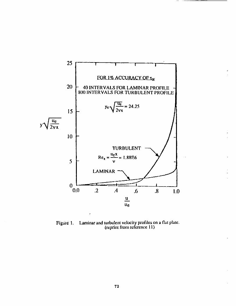
lleY 2vx
25
20
15
10
5
00.0
I ! I I" ;' i
!
8110 INTERVALS FOR TURBULENT PROFILE]
/Ye_2_x = 24.25
q_RBULENT --_ / ]
.2 .4 .6 .8 ! .0
U
U¢
Figure 1. Laminar and turbulent velocity profiles on a fiat plate.(reprint from reference 11)
72
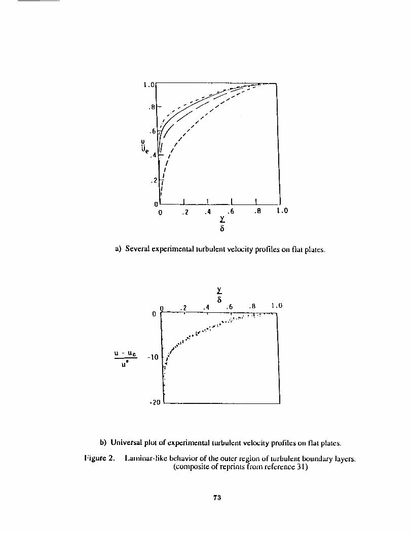
!.0
.8
U
Oe.4
II
.2 i-I!
0 L0
/
/ /-- I
/
I _ I I.2 .4 .6 .8
7...0
a) Several experinaental turbulent velocity profiles on fiat plates.
U - U B
U
-10
-20
b) Universal plot of experimental turbulent velocity profiles on llat plates.
Figure 2. l.aminar-like bcllavior of the outer region of tmbulent boundary layers.(composite of reprints from reference 31 )
73

0 I I I !0 I 2 3 4
Y uc
c) Solulion_ of lhe Blasius equation with nOnzero surfa_ velocities.
u - Ue tOU*
I .2 .40 = !
(fig 2c) ..j..t
,o
-20 / i !
Z.s
.6 .8 l
ft
1 I
d) Comparison of the data shown in fig. 2b and 2c.
Figure 2. Concluded.
?4

f' -I0.
13= -0.5
zero-order; outer
zero-order; inner
exact; zero-order
Mellor & Gibson
n
Figure 3. Velocity defect profiles with I_ = -0.5 for incompressible flow.
75

Oi
-5.
F' -10.
-15.
+
O
13=2
I01 & 51 point grid
11 point grid; outer
6 point grid; outer
-20.
0.00 .05 .10 .15 .20 .25
N
.3O
Figure 4. Grid resolution comparisol! for iJ,c(_ml)ressible flow.
76

!
e
-5.
-10.
-15.
u
m
/
//
/
/
,t
/
13=0
0 full eqns; outer
full eqns; inner
- /x zero-order; outerm
zero-order; inner
_ Mellor & GibsonIIlJlJltr!lfJ)ll!lilfJlllllJllllrll!)l!l ]r,]
•05 .10 .15 .20 .25 .30 .35 .40 .45
11
Figure 5.
a) p=0
Velocity defect profiles with 13_<I for incompressible flow.
77

f' -I0.
_a__._k_-_-- _3---_i_---_
o
A
13=0.5
full eqns; outer
full eqns; inner
zero-order; outer
zero-order; inner
Mellor & Gibson
.05 .I0 .15 .20 .25 .30 .35
b) I] = 0.5
Figure 5. Continued.
78

!
/
/
/
/
0
9=1
full eqns; outer
full eqns; inner
zero-order; outer
zero-order; inner
Mellor & GibsonI
.20 .25
c) p=1
Figure 5. Concluded.
79
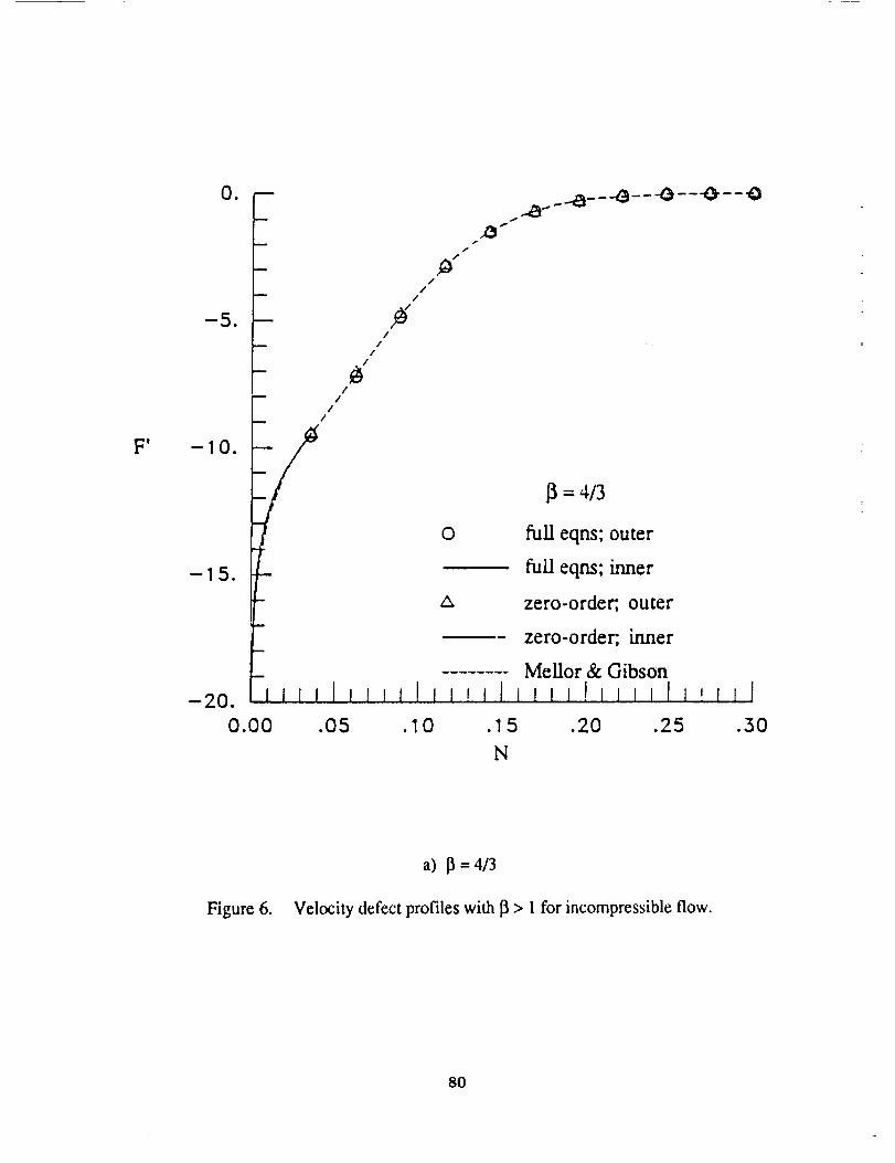
!
O. __-- _._.._._---_---_---_-- 0
--5. m /z_
-- I I
i /
-10.
13= 4/3
[._ o fulleqns; outer
-1 5. F _ full eqns; inner
_ zero-order; outer
--- zero-order; inner
!--- ........ Mellor & Gibson
-20. f l ,
0.00 .05 .10 .15 .20 .25 .30
N
Figure 6.
a) p = 413
Velocity defect profiles with _ > 1 for incompressible flow.
80

!
. m
m
m
I
m
-.5.
-10.
-15.
ff
s"i,
. .0...0-- -_--- O'-- O"--O
I
I
- _/
/
//
0
/x
1_=2
full eqns; outer
full eqns; inner
zero-order, outer
zero-order; inner
MeUor & Gibson
.05 .I0 .15 .20 .25 .30N
b) p=2
Figure 6. Continued.
81
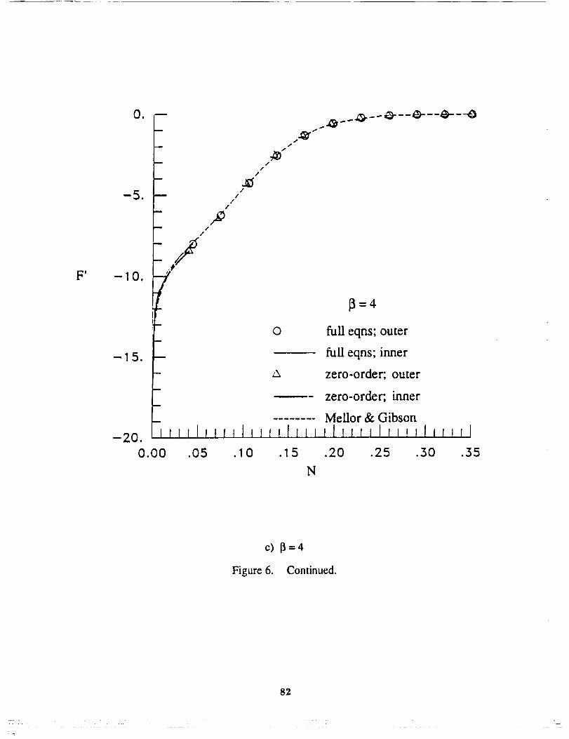
,,
-5.
m
m
u
D
/
/
#,
/
/
//
//
!
13=4
full eqns; outer
full eqns; inner
zero-order; outer
zero-order; inner
MeLlor & Gibson
•05 .10 .15 .20 .25 .30 .35
N
C) _=4
Figure 6. Continued.
82
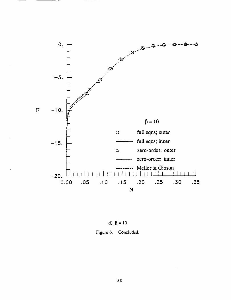
!
Oe
-5.
-10.
a
u
f
p-
f
3"I'
t"
N
d) 13=10
Figure 6. Concluded.
83

Fo.
_=I0
k = 0.0154935
k=0.016
l , I I 1 I I I I I , t J I
-15. -10. -5.
F_
Figure 7. Effect of tile Clauser constant k on convergence with 13= 10
for incompressible flow.
84

Y
\
Re 6. = 105
o fuLl eqns
,x zero-order
c_ Mellor & Gibson
0.0 2.5 5.0 7.5 10.0
Figure 8. Shear-stress velocity ratio comparison with Re6, = 105
for incompressible flow.
85

u+
50.
40.
,30,
20.
10.
O. I
100
F
- _ o lull eqns; outer
lull eqns, trmer_ Mellor & Gibson
r t lrtllt r I _llll_l I '_Jl_tlll I I I lZ_ltl J
1 0 _ 102 103 104
y+
a) Computational comparison with 13= 4 and Res, = 105.
Figure 9. Inner variable profiles for several incompressible cases.
86

U+
50.
40.
30.
20.
10.
o
10 o
m
m
0
m
--+
13= 7.531
full eqns; outer
full eqns; inner
experiment; profile 2305 (ref. 46)
..O
I ! I_'lJlJ I I IIIIII] _ i l llllll
10 _ 10 2 10 3
y+
0
0
"1"
0
b) Comparison with experimental data with j3 = 7.531 and Re,i* = 30,692.5.
Figure 9. Concluded.
87
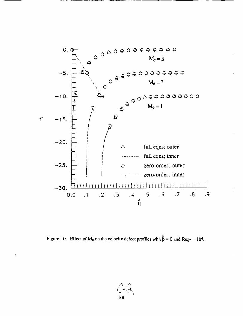
!
\
-- \
-10. -_
E
-15.1
I
_ II
-- II-20. -- il
II
-- I
-25. - I- I
-30. ]!,_l0.0 .1
OOO0000_O000
0 Me=5
\
\
\
\
%,
Me=3
2_ zD1
II
0
.2 .3 .4 .5A
rl
full eqns; outer
full eqns; inner
zero-order, outer
zero-order; inner
!ll!!lllllt,_!!l!!l
.6 .7 .8 .g
,,%
Figure 10. Effect of Me on the velocity defect profiles with _ = 0 and Res. = 104.
88

!
x _ Re6" = 107
-5. _ OOOO_OOOOOOOO105_x\,. Res. =
-I0. "_Z__ 0000_)_)(__000
-20. -- P- _', full eqns; outer
- full eqns; inner
-25. -- O zero-order; outer
- zero-order; inner
-30. "TJJJllJrJlJI lllJftlIIJIllJlJlJliIllfJ l IfIl
0.0 .1 .2 .3 .4 .5 .6 .7 .8 .9A
q
A
Figure 11. Effect of Re6. on the velocity defect profiles with Me = 3 and 13= 0.
89

|
o
-5.
-10.
-15.
-20.
-25.
-30.
-'_-. O- Om %.
%m
%%
,%m ,%
_,t!
B
m
i
i
%
"®
OOOOOOOOOOOA
]3=0
m
i
i
m
m
w
m
m
-35. -IrJI]J_
0.0 .1 .2
13--!,_o
Q
l'l
& full eqns; outer
full eqns; inner
0 zero-order; outer
zero-order; inner
JtllJllllJJlfl]JIIJlII!ll
.3 .4. .5 .6 .7A
q
P,
Figure 12. Effect of [] on the velocity defect profiles with Mc = 3 and Res* = 104.
9O

h
numerical, eqn (4.2)
analytical, eqn (2.9)
Me=O Me=2A
Me=4
1
0.0 .2 .4 .6 .8 1.09
ul
rl
A
Figure 13. Analytic and numeric values of the law of the wake with 13= 0 and Re8. = l0 4.
91

W
200.Ao--
rl-- 13=0A
0 13=IA
15o. A 13=2A
_ p=4
_- X analytical, eqn (4.3)
100.
0. I. 2. 5. 4.
Me
A
a) Effect of 13and Me with Re_i. = 104.
Figure 14. Behavior of the the law of the wake coefficient.
92
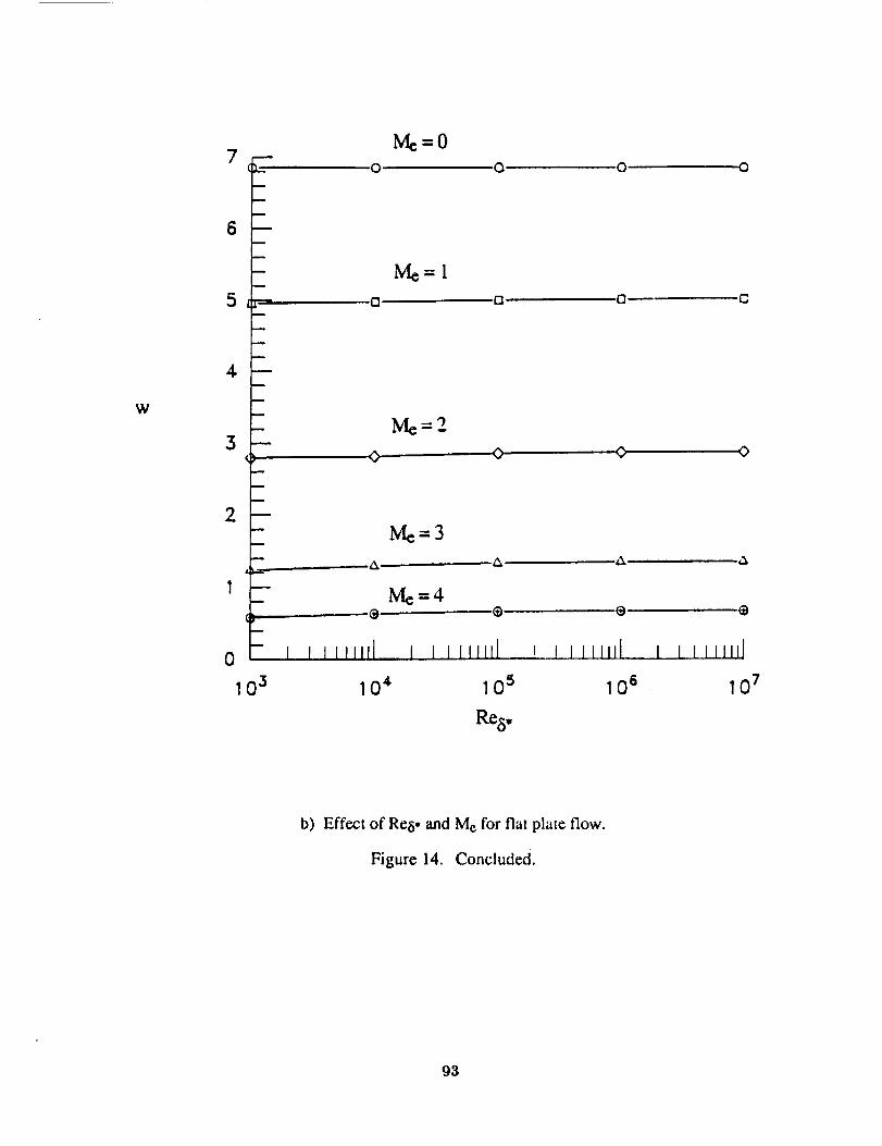
W
7
6
5
4
3
2
0
m
t.. O
Me=0
m
m
m
- Me=lw
F" rlm
m
m
m
- Me=2m
m
m
m
- Me=3
i=--
--- Me=4
- t I J ttJtfi i I
10 3 10 4
Q 0 O
o o m
0 ¢ 0
A, A ,_
j[II))l , ) J filJJl
i0 s 10 8
Re8•
G
[ l II Illll
10 7
b) Effect of Re_i. and Me for fiat plate flow.
Figure 14. Concluded.
93

FI
10 2 m--=.i.
Eo!
w
10 1
i
i
100I
F10-I
I0 -t
numerical
eqn (4.4)
t I I ItIJ_l r _ i itr,iI l ! LL'Ifll
I0 0 101 I021
13+ .
a) Comparison of analytical and numerical values of I-1.
Figure 15. The incompressible law of the wake coefficient.
94
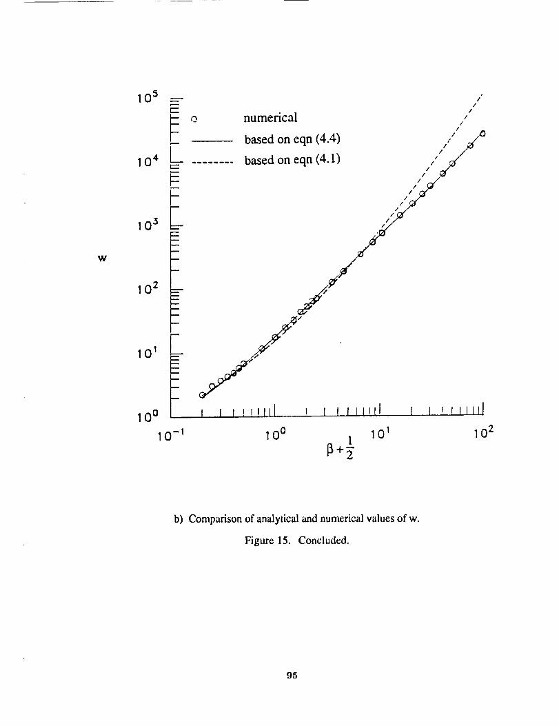
W
10 5
E 0
10 4 1
10 3 =-
1 0:2 ---
101 _--
I 0 °
I0 -I
numerical
based on eqn (4.4)
based on eqn (4.1)
/
//
//
/
I/I/ "_
////
/
j/-
/I _ _ !!!/11 _ 1 I II1!1!
10 0 101I
I I !lllll]
10 2
b) Comparison of analytical and numerical values of w.
Figure 15. Concluded.
95

O_
2.5
m
i
m
2.0 --m
1.5
1.0 --
m
m
i
0.0 1
-2.5
,..%
ga
b
o Q 0
o _=t
= _=2
o _=3
,x _ =4
eqn (4.5)
IIJJlJlllll lltf!,l frl]
0.0 2.5 5.0 7.5 10.0A
^
Figure 16. Effect of 13on the law of the wake coefficient exponent ix.
96

!
1
-5.
-10.
y- 0
/m/
13=0
Re 6. = 10 4
_u
32 point grid
+ 12 point grid
o 7 point grid
•1 .2 .3 .4. .5 .6 .7A
q
Figure 17. Grid resolution comparison for compressible flow.
97

e
Oe
-5.
-10.
-15.
-20.
0.0
i!
®
Me=3
Re 5, = 104
JILl I,IJr llJlullJfJlllJllfJltlllf
Figure 18.
a) Effect on velocity defect profiles.
A
Effect of 13on various profiles with Me = 3 and Re,i. = 10 4.
g8

am
u_
.6
.4
I
.2
Me= 3
Reg. = 104
O_ _ =-0.3
b) Effect on velocity profiles.
Figure 18. Continued.
9g

.P._Pe
Me=3
Res. = I0 ¢
[3 = -0.3
= -0.15
{3=IA
o.o ])_)l_tlil,,J,lll!ll,,),lr_ll)[_tll)_,lJJ),l0.0 .1 .2 .3 .4 .5 .6 .7 .8 .9
A
rl
c) Effect on density profiles.
Figure 18. Concluded.
lOO

!
_=0
Re8, -- 10 4
Me=0
Me=l
Me=2
Me=3
Me=4
a) Effect on velocity defect profiles.
A
Figure 19. Effect of Me on various profiles with _ = 0 and Res° = 104.
101

U
Ue
1.0
.8
.6
m
m
m
I
m
Re6, = 104
A
b) Effect on velocity profiles.
Figure 19. Continued.
102

P_..pc
1.0
.8
.6
.4
.2
- o-o-o-.%_r._.; -_.- ' •u /t_ A'f.®
-- / /
¢
-- /
- / ReS. = 104-®
A
- _=0
- O-- _=0
- [] _=I
_ 0 _=2
- _, _=3
- _ _=4
tlllllv_llrl11111JlrllllJltl!tfJil
• 1 .2 .3 .4 .5 ,6 .7A
rl
c) Effect on density profiles.
Figure 19. Concluded.
103

-/
0.0 2.5 5.0 7.5 10.0A
A
a) Effect of 13and Me with Reg. = 104.
Figure 20. Behavior of the shear-stress velocity ratio.
104

Y
.O6
.05
.04
.03
.02 --
.01 --
0
103
o--_=0
o-- IV_=l
o Me=2
A-- Me=3
Me=4I I I [I Iltl 1
10 4
I I r llJJl I J if Jt!ll .t t ,l I_lll
I0 s 10 6 10 7
Res,
b) Effect of Res* and Me for flat plate flow.
Figure 20. Concluded.
105

Co
2.50
2.25
2.00
1.75
i .50
1.25
1.00
.75
.5O
.25
m
m
u
m
m
m
m
4._/&"
_9.o.oIo______-o o. o o
EIOID-O-O_O O 0 '0 , 0
OIX)-O-O_O- O- O-- 0 0
o- Me:O
o -Me=l
o-------- Me = 2 Res. = 10 4
' Me=3
-s' _=4
I
0 2.5 5.0 7.5 10.0A
A
a) Effect of _ and Me with Re/i. = 104.
Figure 21. Trends of the compressibility parameter ta.
106

03
2.00 __1.75 ®_
1.25
A__,'X
-
l .00
.75 --
.50 --
.25 --
0 -
103
_0 [] O 0•0 .0 0 0
,m
0
Q
Me=0
lVle= t
Me=2
Me= 3
Me=4
13=0
I J llIIIIl j f j f,_IIl I J
10 4 105
1 I llllJ
106
I I I 111111
10 7
Re 6.
b) Effect of Re6. and Me for flat plate flow.
Figure 21. Concluded.
107

t
Oa
-5.
-10.
-15.
m \
-- \\ +
\
m C_\\
1. \
- g
"t"
r,
*o1.
0 0
+
0
6-4-
Q
0
0 0 0 0 0 0
Me=4.544
Re 8. = 902
00000
Me = 2.578
Re_5, = 5295
O O
000
I-
- l:f.
/ -I-
0
experiment
zero-order; inner
zero-order; outer
_lllltl IllvlllJllllllllllvJllllJJllJltlJlJll
• 1 .2 .3 .4 .5 .6 .7 .8 .9A
Figure 22.
a) Comparison of velocity defect profiles.
Comparison of various profiles with experimental data for compressible flowon a fiat plate.
108

Um
ue
1.0
.8
.6
.4
.2
\m\
m -t. \
L
m
m
m
m
m
+o +oP
\\\
\
0+
Q+
(j- 0 0 0 0 0 0 0 0 0 0
Me =4.544
Re 8. = 902
+
b+o OOOOOOMe = 2.578
Re 8. = 5295
oooo
+ experiment
zero-order; inner
0.0
0.0
0 zero-order; outer
•I .2 .3 .4 .5 .6 .7 .8 .91%
q
b) Comparison of velocity profiles.
Figure 22. Continued.
109
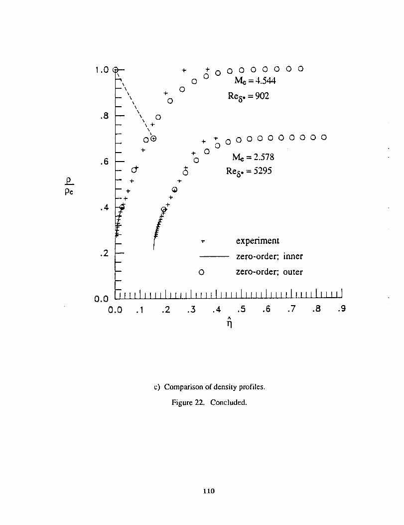
P_..Pe
1.0
.8
.6
.4
.2
\
\m \
\i
4-
i
4-
0\\
\ 0\\4-\
4-
4-
(P4"
4-
0
0
4-
0
+0 0 0 0 0 0 0 0 0
M_=4.544
Re 6. = 902
+ ; 0000000000
0M, = 2.578
t
Re 6. = 5295
O
experiment
zero-order; inner
zero-order; outer
c) Comparison of density profiles.
Figure 22. Concluded.
110

.030
.025
.020
Y.015
(meters)
.010
-- 0
- o baseline, 51 points oo
-- 0
- o slip-vel_ity, 26 points-- 8
- empirical inner solution om
- + experiment 8
Oo
-- o
N
O
-- O
-- %
0
i
Me = 2.578 d*"
•005 _-- Re6" = 5295 _,eo,._°,8 "
o Fl I, .ilv l_,,.L,_,._,l Ill
0 .2 .4. .6 .8 1.0
U
u¢
a) Velocity ratio comparison.
Figure 23. Baseline and slip-velocity Navier-Stokes solutions for Me = 2.578.
111

.025
.020
Y.015
(meters)
.010
.030 --m
-- 0
-- o
m
.OO5
0
baseline, 51 points
slAp-velocity, 26 points
empirical inner solution
experiment
- Me = 2.578
Re 8. = 5295
u
m
m
1
0
1,'!l tiLl.2 .4
O
oO
8
O
8
0
Oo
qb
oo
o
o
o
o0
o o
0
o_4"
0
'1_!1
.6 .8 I .0
b) Density ratio comparison.
Figure 23. Concluded.
112

.030
.025
.O2O
Y.015
(meters)
.010
.005
0
m
-- 0
m
m 11.
m
m
m
m
m
n
m
m
N
Me = 4.544
Re 8. = 902
baseline, 51 points
slip-velocity, 26 points
empirical inner solution
experiment
m
_lel
0
0
0
oo
8
0
8
0o
0
o
0
g
d_
0
.6 .8
u
tle
a) Velocity ratio comparison.
Figure 24. Baseline and slip-velocity Navier-Stokes solutions for Me = 4.544.
113
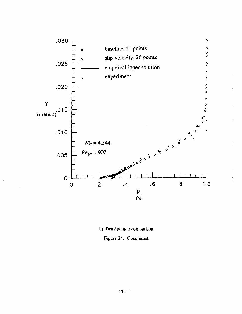
.030
.025
.020
Y.015
(meters)
.010
.005
0
m 0
0
o0
empirical inner solution a0
_ , experiment a
Oo
-- Om
O
m O
-- g
0 0
0 t-
O0
0 I.0
0
- Me = 4.544 o0 0t"
0
- Res, = 902 %m _ o
i t i I I'-__, I J J J _ I I I I J I ,, , _ I
baseline, 51 points
slip-velocity, 26 points
0 .2 .4. .6 .8 I .0
P_Pe
b) Density ratio comparison.
Figure 24. Concluded.
114

_alo_aJ AP_of_ul_ and_:_C e Z_r_trMSllaT_
1. Report No.
NASA CR-4286
4. Title and Subtitle
Report Documentation Page
2. Government Accession No. 3. Recipient's Catalog No.
5. Report Date
Development of a Defect Stream Function,Law of the Wall/Wake Method for CompressibleTurbulent Boundary Layers
7. Author(s)
Richard A. Wahls
9. Pedorming Organization Name and Address
North Carolina State UniversityDepartment of Mechanical and AerospaceRaleigh, NC 27695-7910
Engineering
12. Sponsoring Agency Name and Address
National Aeronautics andLangley Research CenterHampton, VA 23665-5225
Space Administration
March 1990
6. Performing Organization Code
8. Performing Organization Report No.
10. Work Unit No.
505-60-01-02
11. Contract or Grant No.
NCC1-117
13. Type of Report and Period Covered
Contractor Report
14. Sponsoring ,_,gency Code
15. Supplementary Notes
The information presented in this report was offered as a dissertationfulfillment of the requirements for the Degree of Doctor of Philosphy,Carolina State University, Raleigh, North Carolina, 1989.
Langley Technical Monitor: David H. Rudy
in partialNorth
16.AbstractThe method presented is designed to improve the accuracy and computationalefficiency of existing numerical methods for the solution of flows withcompressible turbulent boundary layers. A compressible defect stream functionformulation assuming an arbitrary turbulence model is derived. Previous problemswith the defect formulation are eliminated by using empirically based analyticexpressions to define the flow near the wall. The need for an inner-region eddy-viscosity model is completely avoided. The near-wall analytic expressions arepatched to numerically computed outer-region solutions at a point determinedduring the computation. A new surface boundary condition is presented; thiscondition replaces the no-slip condition and enables numerical integration to thesurface with a relatively coarse grid. The method has been evaluated forincompressible and compressible equilibrium flows and has been implemented intoan existing Navier-Stokes code.
17. Key Words (Suggested by Author(s))
Law of the WallLaw of the WakeEquilibrium Boundary LayerTurbulent Boundary LayerCompressible Flow
18. Distribution Statement
Unclassified-Unlimited
Subject Category 34
19. Security Classif. (of this report)
Unclassified
_. Security Cla_if. (of this page)
Unclassified
21. No. of pa_s _. Price
124 A06
NASA FORM 1626 OCT 86
For sale by the National Technical Information Service, Springfield, Virginia 22161-2171NASA-Lan_,I990
