○E

Report on the August 2012 Brawley EarthquakeSwarm in Imperial Valley, Southern Californiaby Egill Hauksson, Joann Stock, Roger Bilham, Maren Boese, XiaoweiChen, Eric J. Fielding, John Galetzka, Kenneth W. Hudnut, Kate Hutton,Lucile M. Jones, Hiroo Kanamori, Peter M. Shearer, Jamie Steidl, JerryTreiman, Shengji Wei, and Wenzheng Yang

Online Material: Tabulation of parameters of the finite sourcemodel for the Mw 5.4 earthquake; tabulation of stress drops,including the event ID and other earthquake parameters.

INTRODUCTION

The 2012 Brawley earthquake swarm occurred in the BrawleySeismic Zone (BSZ) within the Imperial Valley of southernCalifornia (Fig. 1). The BSZ is the northernmost extensionalsegment of the Pacific–North America plate boundary system.Johnson and Hill (1982) used the distribution of seismicitysince the 1930s to outline the geographical extent of theBSZ, defining boundaries of the BSZ as shown in Figure 1. Itsnorth–south extent ranges from the northern section of theImperial fault, starting approximately 10 km north of theUnited States–Mexico international border and connecting tothe southern end of the San Andreas fault, where it terminatesin the Salton Sea. Larsen and Reilinger (1991), who defined asimilar geographical extent of the BSZ, argued that the BSZ wasmigrating to the northwest, which they associated with thepropagation of the Gulf of California rift system into theNorth American continent.

During the seismically active period of the 1970s, theBSZ produced close to half of the earthquakes recorded inCalifornia (Johnson and Hill, 1982; Hutton et al., 2010).However, for two decades following the 1979 Imperial Valleymainshock Mw 6.4 and its aftershock sequence, the BSZ wasmuch less active. In general, the BSZ seismicity is indicative ofright-lateral strike-slip plate motion accompanied by crustalthinning as well as possible associated fluid movements inthe crust (Chen and Shearer, 2011).

The 2012 Brawley swarm produced more than 600 eventsrecorded by the United States Geological Survey (USGS)–California Institute of Technology (Caltech) SouthernCalifornia Seismic Network (SCSN). Other monitoring instru-ments in the region, such as the Global Positioning System(GPS) network, creepmeters, and the Wildlife LiquefactionArray (WLA) also recorded signals from the largest events. In

addition, Interferometric Synthetic Aperture Radar (InSAR)satellites collected images from space.

THE 2012 BRAWLEY SWARM

The 2012 Brawley swarm started near the town of Brawley at4:30 (UTC) on 26 August, with three events of Mw > 5occurring within 5 min. The seismic activity picked up againat 11:43 (UTC) and continued at a steady rate. The three larg-est earthquakes (Mw 5.3,Mw 4.9, andMw 5.4) in the sequenceoccurred over a period of 90 min, starting at 19:31 (UTC).The largest (Mw 5.4) earthquake was widely felt across south-ernmost California, northern Baja California, and western Ari-zona. The SCSN ShakeMap showed strong to very strongshaking within a 10-km distance of the epicenter (http://www.cisn.org).

The causative fault of the 2012 swarm had not been pre-viously mapped. Nonetheless, surface fractures that are relatedto the swarm were identified both from InSAR images andfield observations. Prior occurrences of surface faulting in as-sociation with swarm activity within the BSZ activity includethe 2005 swarm (Lohman and McGuire, 2007; Rymer et al.,2011). The largest event of the 2005 swarm was Mw 5.1, yetsurface rupture was up to 20 cm in that case. Similarly, the2006 Cerro Prieto swarm with the largest event ofMw 5.4 hadsurface rupture along the Morelia fault of 20–30 cm (Suárez-Vidal et al., 2007). Also, just to the west of the BSZ, the ElmoreRanch event MS 6.2 of the 1987 Superstition Hills sequenceinvolved extensive surface rupture on a zone of cross-faults(e.g., Hudnut et al., 1989; Sharp et al., 1989).

In this report, we summarize the recent data and interpre-tations for this sequence. In particular, we highlight efforts to(1) find the surface rupture; (2) develop a finite source mod-eling using both seismic and GPS waveforms, together with(3) data from creepmeters; and (4) a liquefaction array. Thetemporal and spatial evolution and focal depths of the eventsare very important for understanding the crustal deformationprocesses that cause such swarms.

doi: 10.1785/0220120169 Seismological Research Letters Volume 84, Number 2 March/April 2013 177

MAINSHOCK MOMENT TENSOR

The SCSN automated analysis of waveforms determined thefirst version of the real-time SCSN moment tensor. Clintonet al. (2006) described the implementation of the method thatwas initially developed by Dreger and Helmberger (1993).Subsequently, several other moment tensors were created,which are listed in Table 1.

Moment tensors provide the depth of the centroid ofmoment release, whereas the P- and S-arrival times providethe hypocenter depth or the depth of rupture initiation, oftendifferent from the depth of the centroid. In the regional sol-utions, the minimum misfits between real and synthetic wave-forms constrain the centroid depth at ∼5 km and the Mw at5.5. The teleseismic centroids tend to be deeper, in part,because the depth resolution is less. Chu and Helmberger(2013) also determined a regional double-couple solution usingthe “cut-and-paste” method (Zhu and Helmberger, 1996) aswell as a local velocity model appropriate for the Imperial Val-ley basin. They found that using a local velocity model, theyneeded a depth of ∼4 km for the centroid. In comparison, thehypocentral depth of the mainshock from the P- and S-arrivaltimes is 6.9 km, located near the bottom of the finite slip dis-tribution.

A new regional W -phase inversion method, based on theteleseismic approach of Kanamori and Rivera (2008), using 34broadband components of SCSN stations with passband of50–150 s, yielded a similar mechanism as the SCSN real-timemethod. For the regional W -phase method, Green’s functionswere generated using the frequency wave number (FK) tech-nique (Zhu and Rivera, 2002) and a 1D southern Californiavelocity model (Zhao and Helmberger, 1994). The teleseismicW -phase and Centroid Moment Tensor solutions, which re-present long-period properties of the source, provided anaccurate moment tensor but poorly constrained centroiddepths in the range of 12 km (see also http://earthquake

▴ Figure 1. The seismicity from 1981 to 2012 August is shown asblack open circles, and the events of the 2012 August Brawleyswarm are shown as red circles. Lower-hemisphere focal mech-anisms of the Mw > 5 events are shown. IRC, Imler Road creep-meter; WLA, Wildlife Liquefaction Array. The east and westboundaries of the BSZ as defined by Johnson and Hill (1982)are shown as red dashed lines. Late Quaternary fault traces (ma-genta) from Jennings and Bryant (2010) are also shown.

Table 1Preferred Nodal Plane for the Largest (Mw 5.4) Earthquake in the Swarm

Mw

CentroidDepth (km) Strike Dip Rake Source/Method

5.44 5.0 233° 66° NW* −22° SCSN† (Dreger and Helmberger, 1993)5.48 11.5 238° 74° NW −11° W -phase regional5.5 11.0 228° 74° NW −45° USGS teleseismic W phase5.4 12.0 232° 67° NW −12° Global CMT5.44 6.9‡ 227° 82° SE 6° Focal mechanism from first motions and S= P ratios5.4 5.5 238° 87° NW −7° Regional cut-and-paste method (Chu and Helmberger, 2013)5.4 4.0 239° 90° 1° Teleseismic cut-and-paste method (Chu and Helmberger, 2013)

*NW, dips to the northwest; SE, dips to the southeast.†SCSN, Southern California Seismic Network; USGS, United States Geological Survey; CMT, Centroid Moment Tensor.‡Hypocentral depth from arrival times.

178 Seismological Research Letters Volume 84, Number 2 March/April 2013

.usgs.gov/earthquakes/eqarchives/fm/ci15200401_wmt.php andhttp://www.globalcmt.org/CMTsearch.html).

In general, all of the moment tensors and the first-motionmechanisms exhibited similar strike-slip motion with a minornormal component on a steeply dipping southwest-strikingnodal plane. This plane coincided with the trend of the mainaftershock distribution. The agreement between the momenttensor solutions, including teleseismic and regional approaches,suggests that the rupture had an ordinary duration for itsseismic moment. However, the differences in local velocitystructure used by each method involve trade-offs between dipand rake, resulting in slightly different parameters. The valuesof all of these parameters are within the expected range ofuncertainty.

SURFACE RUPTURE OR FRACTURES

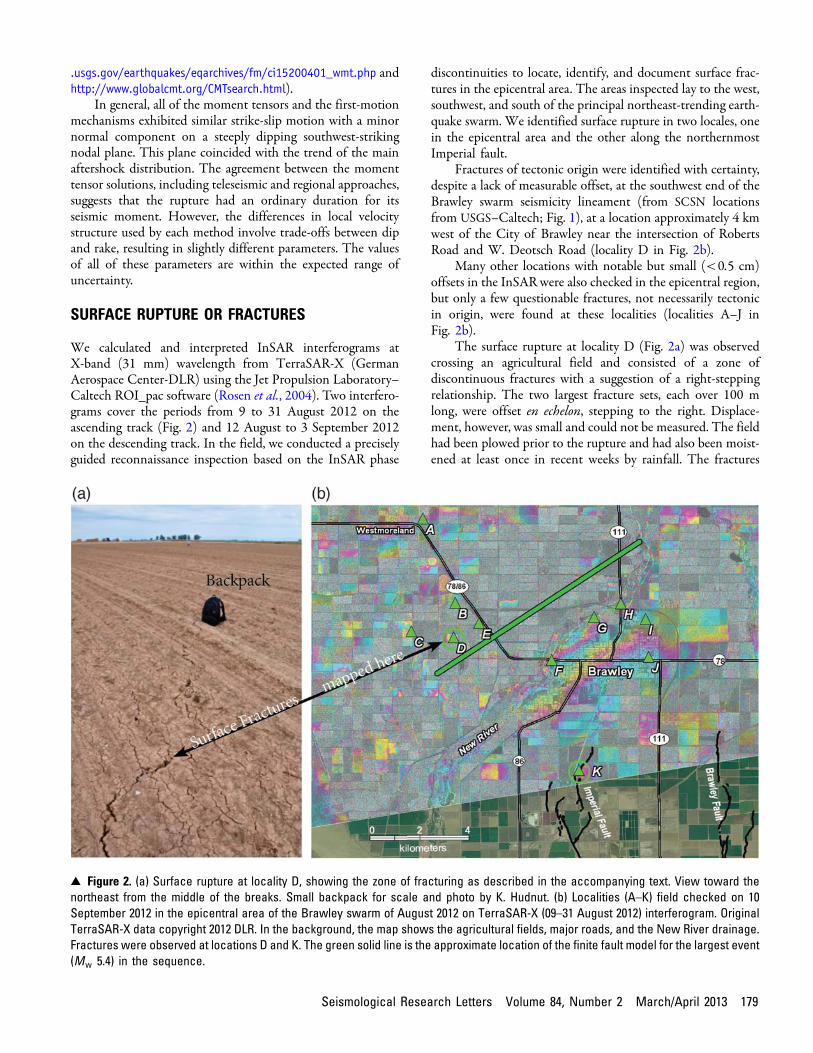
We calculated and interpreted InSAR interferograms atX-band (31 mm) wavelength from TerraSAR-X (GermanAerospace Center-DLR) using the Jet Propulsion Laboratory–Caltech ROI_pac software (Rosen et al., 2004). Two interfero-grams cover the periods from 9 to 31 August 2012 on theascending track (Fig. 2) and 12 August to 3 September 2012on the descending track. In the field, we conducted a preciselyguided reconnaissance inspection based on the InSAR phase

discontinuities to locate, identify, and document surface frac-tures in the epicentral area. The areas inspected lay to the west,southwest, and south of the principal northeast-trending earth-quake swarm. We identified surface rupture in two locales, onein the epicentral area and the other along the northernmostImperial fault.

Fractures of tectonic origin were identified with certainty,despite a lack of measurable offset, at the southwest end of theBrawley swarm seismicity lineament (from SCSN locationsfrom USGS–Caltech; Fig. 1), at a location approximately 4 kmwest of the City of Brawley near the intersection of RobertsRoad and W. Deotsch Road (locality D in Fig. 2b).

Many other locations with notable but small (<0:5 cm)offsets in the InSARwere also checked in the epicentral region,but only a few questionable fractures, not necessarily tectonicin origin, were found at these localities (localities A–J inFig. 2b).

The surface rupture at locality D (Fig. 2a) was observedcrossing an agricultural field and consisted of a zone ofdiscontinuous fractures with a suggestion of a right-steppingrelationship. The two largest fracture sets, each over 100 mlong, were offset en echelon, stepping to the right. Displace-ment, however, was small and could not be measured. The fieldhad been plowed prior to the rupture and had also been moist-ened at least once in recent weeks by rainfall. The fractures

▴ Figure 2. (a) Surface rupture at locality D, showing the zone of fracturing as described in the accompanying text. View toward thenortheast from the middle of the breaks. Small backpack for scale and photo by K. Hudnut. (b) Localities (A–K) field checked on 10September 2012 in the epicentral area of the Brawley swarm of August 2012 on TerraSAR-X (09–31 August 2012) interferogram. OriginalTerraSAR-X data copyright 2012 DLR. In the background, the map shows the agricultural fields, major roads, and the New River drainage.Fractures were observed at locations D and K. The green solid line is the approximate location of the finite fault model for the largest event(Mw 5.4) in the sequence.

Seismological Research Letters Volume 84, Number 2 March/April 2013 179

were evident as a N45°E-trending zone of wider fractures over-printed on a relatively consistent pattern of dessication cracksalong the north–south furrows. The TerraSAR-X interfero-grams indicate as much as 3 cm of offset across the zone inthis field. It is not possible to tell if the surface displacementoccurred as a coseismic slip or afterslip because the field ob-servations were delayed (10 September 2012).

The second rupture we observed was along the trace of theImperial fault, north of Carey Road (locality K in Fig. 2b).Again, the ground had been moistened by recent rains, butwe were able to observe two localized zones, extending fora total of approximately 20–30 m, of linear discontinuous frac-tures overprinted by the dessication polygons. We judge this torepresent triggered slip along this fault trace. The interfero-grams suggest around 1 cm of slip at this location.

FINITE FAULT MODEL

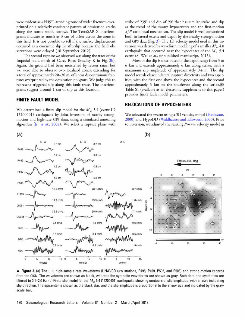
We determined a finite slip model for the Mw 5.4 (event ID15200401) earthquake by joint inversion of nearby strong-motion and high-rate GPS data, using a simulated annealingalgorithm (Ji et al., 2002). We select a rupture plane with

strike of 239° and dip of 90° that has similar strike and dipas the trend of the swarm hypocenters and the first-motionS=P-ratio focal mechanism. The slip model is well constrainedboth in lateral extent and depth by the nearby strong-motionand GPS data (Fig. 3). The 1D velocity model used in this in-version was derived by waveform modeling of a smallerMw 4.0earthquake that occurred near the hypocenter of the Mw 5.4event (S. Wei et al., unpublished manuscript, 2013).

Most of the slip is distributed in the depth range from 3 to6 km and extends approximately 6 km along strike, with amaximum slip amplitude of approximately 0.4 m. The slipmodel reveals clear unilateral rupture directivity and two asper-ities, with the first one above the hypocenter and the secondapproximately 3 km to the southwest along the strike.ⒺTable S1 (available as an electronic supplement to this paper)provides finite fault model parameters.

RELOCATIONS OF HYPOCENTERS

We relocated the swarm using a 3D velocity model (Hauksson,2000) and HypoDD (Waldhauser and Ellsworth, 2000). Priorto inversion, we adjusted the starting P-wave velocity model in

▴ Figure 3. (a) The GPS high-sample-rate waveforms (UNAVCO GPS stations, P498, P499, P502, and P506) and strong-motion recordsfrom the CISN. The waveforms are shown as black, whereas the synthetic waveforms are shown as gray. Both data and synthetics arefiltered to 0.1–2.0 Hz. (b) Finite slip model for theMw 5.4 (15200401) earthquake showing contours of slip amplitude, with arrows indicatingslip direction. The epicenter is shown as the black star, and the slip amplitude is proportional to the arrow size and indicated by the gray-scale bar.

180 Seismological Research Letters Volume 84, Number 2 March/April 2013

the Imperial Valley basin to be approximately 2:5 km=s at 1 kmdepth to account for the low VP velocities in basin sediments(Han et al., 2012). This 3D model can be used to determineaccurate hypocenters because the azimuthal distribution ofstations is fairly complete, but the model needs to be furtherrefined before it can be used for tectonic interpretation. Therelocations reveal a narrow 10-km-long, linear southwest seis-micity trend concentrated in the depth range of 4–9 km(Fig. 4). This trend is aligned along the southwest-strikingnodal plane of the mainshock moment tensors and extendsmostly to the southwest away from the mainshock.

The distribution of focal depths for the swarm earth-quakes is consistent with the finite source model. The eventssurround the two high-slip asperities, with more seismicity nearthe bottom of the large-slip asperity and on the northeast sideand less seismicity near the base of the smaller low-slip asperitylocated 3 km to the southwest. Furthermore, the three largestevents of Mw 5.5, Mw 5.3, and Mw 4.9 are located within ap-proximately 1 km of each other with focal depths of 6.9, 5.7,and 5.2 km, respectively. These focal depths are fairly shallow,but they are typical for this region (Hauksson et al., 2012). Theuncertainties in the depth determinations are small (∼0:7 km)because of the dense distribution of seismic stations in theregion.

The two depth cross sections show the details of the depthdistribution of the earthquakes in the swarm, as well as the VPvelocities in the swarm area. The tight distribution of earth-

quakes in the A–A0 cross section shows that probably the bulkof the swarm events occurred on only one vertical fault. Theseismicity distribution in the B–B0 cross section suggests thepresence of two clusters along this southwest-striking plane,separated by less than 2 km. The VP velocities are low in thenear surface, indicating that the basin sediments bottom at ap-proximately 4–5 km depth. The sediments consist of uncon-solidated clastic sediment from the Colorado River. Thebasement, below the sediments, is interpreted to be metamor-phosed Colorado River sediments, which have been metamor-phosed by the high geotherm (Fuis et al., 1984). The VP of thebasement is lower than that for the average southern Californiabasement because it is more felsic or fractured. The lower crust,as characterized by VP greater than 6:7 km=s, can be seen at adepth of 12 km in the northeast corner of the B–B0 cross sec-tion (Fuis et al., 1984; Han et al., 2012). Improved resolutionof the 3D complexity in the VP structure is expected when theresults of the analysis of the data collected during the SaltonSeismic Imaging Project (SSIP) experiment become available(Han et al., 2012; Rose et al., 2012).

Some off-fault seismicity occurred along an almost north–south strike, extending 10 km away to the south of the mainrupture and 10 km to the north of the rupture, en echelon offsetacross the rupture (Fig. 1). This seismicity occurred within re-gions that have been seismically active during the last 30 years.

FOCAL MECHANISMS

We used first-motion polarities and S=P amplitude ratios andthe HASHmethod of Hardebeck and Shearer (2002, 2003), asimplemented by, to determine focal mechanisms for the eventsin this swarm. There are 13 events ofMw ≥ 3:5 that have A- orB-quality focal mechanisms (Fig. 5). The focal mechanisms ofthe large earthquakes in the sequence are similar to the corre-sponding moment tensor mechanisms for the largest event(Table 1). The focal mechanisms of most of the events pre-dominantly exhibit strike-slip motion on northeast- or north-west-striking nodal planes. Overall, the focal mechanismsuniformly suggest the presence of a coherent regional stressfield.

Along the almost north–south trend of seismicity, normalfaulting is more prominent on either north or north-northeast-striking nodal planes than along the main northeast-trendingaftershock zone. Among the five events ofMw ≥ 2:0 that haveA-quality focal mechanisms (Fig. 5), three of them exhibit nor-mal faulting in north- or north-northeast-striking nodal planes.The current plate boundary right-lateral strike-slip motion, incombination with crustal extension and thinning, causes seis-micity with left-lateral faulting as well as small-scale normalfaulting on north- to north-northeast-striking nodal planes.

EARTHQUAKE STATISTICS

This sequence of earthquakes is described as a swarm because itstarted with a series of small earthquakes, grew in number and

▴ Figure 4. (a) Relocated seismicity, in which the dates of theevents are indicated by the color of the circles. Location of sur-face rupture or fractures as a white and red line, geothermal areaas a triangle, and town of Brawley as inverted triangle are indi-cated. The mapped surface rupture and the Brawley geothermalareas are also shown. Late Quaternary faults are shown in colorcyan. The 3D V P model is modified from Hauksson (2000).(b) Northeast depth cross section. (c) Northwest cross section.

Seismological Research Letters Volume 84, Number 2 March/April 2013 181

magnitude over the first 5.5 hr, and had three events close tothe largest magnitude.

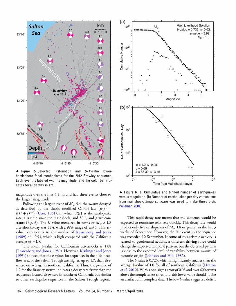
Following the largest event ofMw 5.4, the swarm decayedas described by the classic modified Omori law (R�t� �K �t � c�−p) (Utsu, 1961), in which R�t� is the earthquakerate; t is time since the mainshock; and K , c, and p are con-stants (Fig. 6). The K -value measured in terms of Mw ≥ 1:8aftershocks/day was 55.4, with a 98% range of �3:5. This K -value corresponds to the a-value of Reasenberg and Jones(1989) of −0:94, which is high compared with the Californiaaverage of −1:8.

The mean p-value for Californian aftershocks is 1.08(Reasenberg and Jones, 1989). However, Kisslinger and Jones(1991) showed that the p-values for sequences in the high-heat-flow area of the Salton Trough are higher, up to 1.7, than else-where on average in southern California. Thus, the p-value of1.2 for the Brawley swarm indicates a decay rate faster than thesequences located elsewhere in southern California but similarto other earthquake sequences in the Salton Trough region.

This rapid decay rate means that the sequence would beexpected to terminate relatively quickly. This decay rate wouldpredict only five earthquakes ofMw 1.8 or greater in the last 3weeks of September. However, the last event in the sequencewas recorded 10 September. If some of this seismic activity isrelated to geothermal activity, a different driving force couldchange the expected temporal pattern, but the observed patternis close to the expected level of variability between swarms oftectonic origin (Johnson and Hill, 1982).

The b-value is 0.725, which is significantly smaller than theaverage b-value of 1.0 for all of southern California (Huttonet al., 2010).With a one-sigma error of 0.03 and over 600 eventsabove the completeness threshold, this low b-value should not bean artifact of incomplete data. The low b-value suggests a deficit

▴ Figure 5. Selected first-motion and S= P-ratio lower-hemisphere focal mechanisms for the 2012 Brawley sequence.Each event is labeled with its magnitude, and the color bar indi-cates focal depths in km.

▴ Figure 6. (a) Cumulative and binned number of earthquakesversus magnitude. (b) Number of earthquakes per day versus timefrom mainshock. Zmap software was used to make these plots(Wiemer, 2001).

182 Seismological Research Letters Volume 84, Number 2 March/April 2013

of smaller earthquakes,which is sometimes interpreted as above-average crustal stress conditions (Scholz, 1968).

Overall, the magnitude–frequency statistics are similarto those Kisslinger and Jones (1991) reported for previoussequences in Imperial Valley. However, they differ from thosewe have observed for some other active geothermal areas suchas Coso in eastern California, in which the b-value is ∼1:25.

SPATIAL AND TEMPORAL EVOLUTION

A weighted-least-square method is applied to model thespatial–temporal migration behavior of this swarm based onthe relocated earthquake hypocenters in the depth range from4 to 8 km. This weighting approach accounts for the uppertriangular nature of the time-versus-distance behavior by apply-ing the L1 norm only within a 0.5-hr window and penalizingearlier events more than the late events outside of this window(further details of the method are provided by Chen andShearer, 2011, appendix A).

The seismicity before the first Mw > 5 earthquakemigrated bilaterally along an azimuth of approximately 55°(approximately northeast–southwest) at a velocity of approx-imately 0:5 km=hr (Fig. 7). The first three events (which oc-curred at 4:30 UTC) that were significantly separated in timefrom the main sequence (approximately 8 hr later) did notshow migration and were not included in the velocity calcu-lation. The southwest migration stopped after the firstMw > 5 earthquake, but the northeast migration continueduntil the second Mw > 5 earthquake.

Four smaller swarms before 2009 (1983, 1986, 1999, and2008) occurred in the same region (Chen and Shearer, 2011).The most recent one in 2008 had a roughly similar migrationvelocity of 0:3 km=hr. Each of these swarms exhibited eitherbilateral or unilateral migration directions, with three swarmshaving unilateral southwestward migration.

Estimated stress drops for the 2012 swarm earthquakesshow a fair amount of scatter, ranging from 0.05 to 1.4 MPafollowing a log-normal distribution. The stress drops are com-puted using the method described in Shearer et al. (2006), inwhich an empirical Green’s function (EGF) is obtained byfitting a Brune-type source model to binned source spectra at0.2-magnitude intervals. When EGFs are computed for subsetsof the data using temporal or spatial binning, the stress dropestimates exhibit some degree of instability in their medianvalues and also with different magnitude bin ranges. The originof these instabilities warrants further study. However, when allevents from 1981 to 2012 are included, the results are consis-tent and stable, with a median value of 0.25 MPa, agreeing withthe values obtained in Chen and Shearer (2011).Ⓔ Table S2(see electronic supplement) provides the tabulation of stressdrops.

PREVIOUS SEISMICITY

During the past 80 years of SCSN earthquake monitoring, theBSZ has been known for its high rate of both mainshock–aftershock and swarm sequences (Johnson and Hutton, 1982;Hutton et al., 2010). During the 1970s, the whole length of theBSZ was dominated by swarm activity. The largest recent main-shock to occur in the BSZ was theMw 6.4 1979 Imperial Valleymainshock, which had an epicenter just south of the Mexico–United States international border and extended to 33.03° inthe north (Johnson and Hill, 1982). In late 1979, a cluster ofaftershocks, with the largest event of Mw 5.8, occurred withinthe region of the 2012 swarm. The Mw 6.4 mainshock wasfollowed by an average aftershock sequence lasting only fora few years. During the period from 1986 to 1999, seismic qui-escence dominated the region. The quiescence was terminatedby several swarms in late 1999 and early 2000 (Fig. 8).

The completeness of the SCSN catalog in the regionimproved with time as seismic stations were added to improvecoverage (Hutton et al., 2010). A major improvement tookplace in 2008when the SCSNbegan recording data from a densenetwork of stations around the south end of the Salton Sea.

The two seismicity clusters that begin forming in the late1980s, at the south shore of the Salton Sea, are related to thegeothermal areas. The production of geothermal energy startedat that time and has resulted in steady seismicity in the region.The seismicity is expressed as two geographically separatedistributions in Figure 8.

The April 1981 Westmoreland swarm occurred 15 km tothe north-northwest of Brawley. It was characterized by astrike-slip-faulting mainshock of Mw 5.8 followed bynumerous aftershocks, forming a left-lateral northeast trend.The 2005 Obsidian Butte sequence ruptured across the

▴ Figure 7. (a) Epicenters shaded in gray by time of occurrence.Arrow indicates the bilateral migration direction, away from thefirst hypocenter in the sequence. (b) Depth versus distance alongthe bilateral migration direction from the first hypocenter. (c) Thespatial and temporal migration of the hypocenters. The smallerblack star is the first Mw > 5 event (Mw 5.3); the larger star isthe second Mw > 5 event (Mw 5.4). In all three figures, eventsare shaded in gray by time as indicated in the gray scale bar.

Seismological Research Letters Volume 84, Number 2 March/April 2013 183

geothermal fields near the southern end of the Salton Sea(Fig. 1). The sequence exhibited swarm-like behavior, andLohman and McGuire (2007) attributed its migration patternto a slow aseismic slip event at depth.

MEASURED TRIGGERED SLIP

Earthquakes on major faults in southern California frequentlytrigger minor amounts of surface slip on nearby and distantfaults, especially those faults that between seismic eventsexhibit aseismic surface creep. Prior to the Brawley swarmin 2012, the Mw 7.2 El Mayor–Cucapah earthquake of2010 triggered slip on dozens of surface faults, some of whichhad not previously been mapped (Rymer et al., 2011).Although earthquakes in the BSZ have never before been ob-served to trigger slip on nearby faults, creepmeters can detectvery small events of slip even when these are not evident in thefield. In 2012, eight creepmeters were operating, four on thesouthern San Andreas fault, two on the northernmost splays ofthe Laguna Salada fault, one on the southernmost Imperialfault near the Mexican border, and one on the SuperstitionHills fault. Each creepmeter has a least-count resolution of≈12 μm and a sampling rate of 30 min (Bilham et al., 2004).The records from these eight creepmeters indicate that trig-gered slip occurred only on the creepmeter crossing the Super-stition Hills fault closest to the swarm (near Imler Road at32.930° N, 115.701° W), where it was manifest as two discreteevents during the largest earthquakes in the swarm. TheMw 5.3 earthquake at 19:31 UTC resulted in 98� 12 μm

of slip, and the larger Mw 5.4 earthquake at 20:57 UTC re-sulted in 49� 12 μm of slip (Fig. 9), a cumulative offset of0:15� 0:02 mm. Our 30-min sampling rate does not permitus to judge the precise time the offset occurred, but in pastevents, it has typically accompanied the passage of surfacewaves (Bodin et al., 1994). This slip is too small to detecton the interferograms.

The fault slip events occurred 1 min after a data sample(Mw 5.3) and the Mw 5.4 earthquake (with half the triggeredslip) 3 min before a sample. No subsequent slip on the fault hasoccurred in the month following the swarm. Slip on the BSZwould place the creepmeter close to a node in the shear-strainfield, suggesting that the slip triggering was not caused byalmost instantaneous static strain but by dynamic shaking.

STATIC STRESS CHANGE

To explain the effects of the largest (Mw 5.4) earthquake in theBrawley sequence on nearby faults and off-fault triggered seis-micity,we determine the static Coulomb stress changes using theapproach of Lin and Stein (2004) and Toda et al. (2005). Forthe slip, we used a 15-cm average slip from the finite sourcemodel over the mainshock fault plane as defined by aftershocks.This fault model extended for a distance of 6.8 km to the south-west and a distance of 3.2 km to the northeast from theMw 5.4event hypocenter over a depth range of 3.0–7.0 km.

We assumed a regional stress direction of N16° E (W.Yang and E. Hauksson, unpublished manuscript, 2013), a fric-tion coefficient on receiver faults of 0.4, Poisson’s ratio of 0.25,

▴ Figure 8. Seismicity in the BSZ from 1970 to 2012. The 2012Brawley swarm is shown as red circles. The seismic quiescencein late 1980s through the 1990s is indicated by a red ellipse. Thetemporal seismicity trends related to geothermal areas aremarked with arrows.

▴ Figure 9. Data from the graphite rod creepmeter on the Super-stition Hills fault near Imler Road 2004–2012 (location IRC in Fig. 1).Dextral slip is indicated by the black line, and the gray line indi-cates temperature in the instrument vault. (inset top) Close-upview of slip triggered on the Superstition Hills fault (solid line) cor-rected for temperature (dotted line). Tick marks on trace indicatesampling interval. Total offset was 0.15 mm.

184 Seismological Research Letters Volume 84, Number 2 March/April 2013

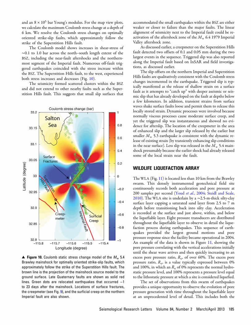
and an 8 × 105 bar Young’s modulus. For the map view plots,we calculate the maximumCoulomb stress change at a depth of6 km. We resolve the Coulomb stress changes on optimallyoriented strike-slip faults, which approximately follow thestrike of the Superstition Hills fault.

The Coulomb model shows increases in shear-stress of∼0:1 to 1.0 bar across the north–south length extent of theBSZ, including the near-fault aftershocks and the northern-most segment of the Imperial fault. Numerous off-fault trig-gered earthquakes coincided with the stress increase withinthe BSZ. The Superstition Hills fault, to the west, experiencedboth stress increases and decreases (Fig. 10).

The seismicity formed scattered clusters within the BSZand did not extend to other nearby faults such as the Super-stition Hills fault. This suggests that small slip surfaces that

accommodated the small earthquakes within the BSZ are eitherweaker or closer to failure than the major faults. The linearalignment of seismicity next to the Imperial fault could be re-activation of the aftershock zone of the Mw 6.4 1979 ImperialValley aftershock zone.

As discussed earlier, a creepmeter on the Superstition Hillsfault detected two offsets of 0.1 and 0.05 mm during the twolargest events in the sequence. Triggered slip was also reportedalong the Imperial fault based on InSAR and field investiga-tions, as discussed earlier.

The slip offsets on the northern Imperial and SuperstitionHills faults are qualitatively consistent with the Coulomb stresschanges incremented in the earthquake. Triggered slip is typ-ically manifested as the release of shallow strain on a surfacefault as it attempts to “catch up” with deeper aseismic or seis-mic slip that has already developed on the fault at depths belowa few kilometers. In addition, transient strains from surfacewaves shake surface faults loose and permit them to release thislocally stored strain. Dynamic processes were involved becausenormally viscous processes cause moderate surface creep, andyet the triggered slip was instantaneous and showed no evi-dence for afterslip. The location of the creepmeter in the areaof enhanced slip and the larger slip released by the earlier butsmaller Mw 5.3 earthquake is consistent with the dynamic re-lease of existing strain (by transiently enhancing slip conditionsin the near surface). Less slip was released in theMw 5.4 main-shock presumably because the earlier shock had already releasedsome of the local strain near the fault.

WILDLIFE LIQUEFACTION ARRAY

TheWLA (Fig. 11) is located less than 10 km from the Brawleyswarm. This densely instrumented geotechnical field sitecontinuously records both acceleration and pore pressure at200 samples per second (Youd et al., 2004; Steidl and Seale,2010). The WLA site is underlain by a ∼2:5-m-thick silty-claysurface layer capping a saturated sand layer from 2.5 to 7 mdepth before transitioning back into silty clay. Accelerationis recorded at the surface and just above, within, and belowthe liquefiable layer. Eight pressure transducers are distributedthroughout the liquefiable layer to observe in detail the lique-faction process during earthquakes. This sequence of earth-quakes provided the largest ground motions and porepressure response since the facility became operational in 2004.An example of the data is shown in Figure 11, showing thepore pressure correlating with the vertical accelerations initiallyuntil the shear wave arrives and then quickly increasing to anexcess pore pressure ratio, Ru, of over 60%. The excess porepressure ratio, Ru, is a value typically expressed between 0%and 100%, in which an Ru of 0% represents the normal hydro-static pressure level, and 100% represents a pressure level equalto the lithostatic pressure at which a site is considered liquefied.

The set of observations from this swarm of earthquakesprovides a unique opportunity to observe the evolution of porepressure generation with time throughout the liquefiable layerat an unprecedented level of detail. This includes both the

▴ Figure 10. Coulomb static stress change model of the Mw 5.4Brawley mainshock for optimally oriented strike-slip faults, whichapproximately follow the strike of the Superstition Hills fault. Thebrown line is the projection of the mainshock source model to theground surface. Late Quaternary faults are shown as solid redlines. Green dots are relocated earthquakes that occurred −1to 23 days after the mainshock. Locations of surface fractures,the creepmeter (see Fig. 9), and the surficial creep on the northernImperial fault are also shown.

Seismological Research Letters Volume 84, Number 2 March/April 2013 185

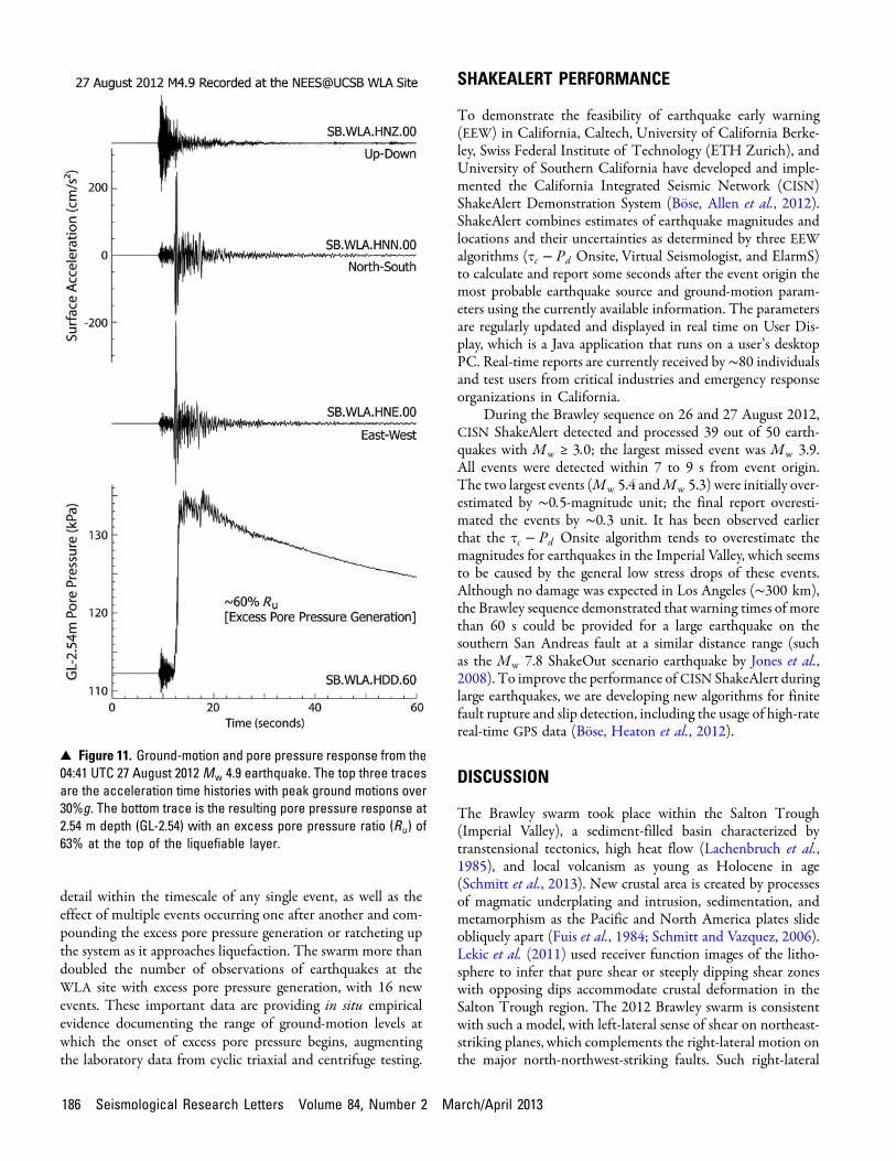
detail within the timescale of any single event, as well as theeffect of multiple events occurring one after another and com-pounding the excess pore pressure generation or ratcheting upthe system as it approaches liquefaction. The swarm more thandoubled the number of observations of earthquakes at theWLA site with excess pore pressure generation, with 16 newevents. These important data are providing in situ empiricalevidence documenting the range of ground-motion levels atwhich the onset of excess pore pressure begins, augmentingthe laboratory data from cyclic triaxial and centrifuge testing.

SHAKEALERT PERFORMANCE

To demonstrate the feasibility of earthquake early warning(EEW) in California, Caltech, University of California Berke-ley, Swiss Federal Institute of Technology (ETH Zurich), andUniversity of Southern California have developed and imple-mented the California Integrated Seismic Network (CISN)ShakeAlert Demonstration System (Böse, Allen et al., 2012).ShakeAlert combines estimates of earthquake magnitudes andlocations and their uncertainties as determined by three EEWalgorithms (τc − Pd Onsite, Virtual Seismologist, and ElarmS)to calculate and report some seconds after the event origin themost probable earthquake source and ground-motion param-eters using the currently available information. The parametersare regularly updated and displayed in real time on User Dis-play, which is a Java application that runs on a user’s desktopPC. Real-time reports are currently received by ∼80 individualsand test users from critical industries and emergency responseorganizations in California.

During the Brawley sequence on 26 and 27 August 2012,CISN ShakeAlert detected and processed 39 out of 50 earth-quakes with Mw ≥ 3:0; the largest missed event was Mw 3.9.All events were detected within 7 to 9 s from event origin.The two largest events (Mw 5.4 andMw 5.3) were initially over-estimated by ∼0:5-magnitude unit; the final report overesti-mated the events by ∼0:3 unit. It has been observed earlierthat the τc − Pd Onsite algorithm tends to overestimate themagnitudes for earthquakes in the Imperial Valley, which seemsto be caused by the general low stress drops of these events.Although no damage was expected in Los Angeles (∼300 km),the Brawley sequence demonstrated that warning times of morethan 60 s could be provided for a large earthquake on thesouthern San Andreas fault at a similar distance range (suchas the Mw 7.8 ShakeOut scenario earthquake by Jones et al.,2008). To improve the performance of CISN ShakeAlert duringlarge earthquakes, we are developing new algorithms for finitefault rupture and slip detection, including the usage of high-ratereal-time GPS data (Böse, Heaton et al., 2012).

DISCUSSION

The Brawley swarm took place within the Salton Trough(Imperial Valley), a sediment-filled basin characterized bytranstensional tectonics, high heat flow (Lachenbruch et al.,1985), and local volcanism as young as Holocene in age(Schmitt et al., 2013). New crustal area is created by processesof magmatic underplating and intrusion, sedimentation, andmetamorphism as the Pacific and North America plates slideobliquely apart (Fuis et al., 1984; Schmitt and Vazquez, 2006).Lekic et al. (2011) used receiver function images of the litho-sphere to infer that pure shear or steeply dipping shear zoneswith opposing dips accommodate crustal deformation in theSalton Trough region. The 2012 Brawley swarm is consistentwith such a model, with left-lateral sense of shear on northeast-striking planes, which complements the right-lateral motion onthe major north-northwest-striking faults. Such right-lateral

▴ Figure 11. Ground-motion and pore pressure response from the04:41 UTC 27 August 2012Mw 4.9 earthquake. The top three tracesare the acceleration time histories with peak ground motions over30%g. The bottom trace is the resulting pore pressure response at2.54 m depth (GL-2.54) with an excess pore pressure ratio (Ru) of63% at the top of the liquefiable layer.

186 Seismological Research Letters Volume 84, Number 2 March/April 2013

motion occurred in the Mw 6.4 1979 Imperial Valley earth-quake. In addition, seismicity that occurred during the Brawleyswarm was induced by a transtensional static stress change, ex-tending approximately 20 km to the south across the Mesquitebasin and approximately 15 km to Westmoreland in the north.Thus, the 2012 swarm activated the BSZ along its whole length,although all of the events were small (Mw < 3). Further north,within the Salton Sea, the seismicity patterns are more sugges-tive of bookshelf faulting (Hauksson et al., 2012).

The nearest major faults with recognized Quaternary sur-face rupture, in the vicinity of the 2012 Brawley swarm, are theImperial and Brawley faults to the south, faults underwater inthe Salton Sea to the north (Jennings and Bryant, 2010), andthe Superstition Hills and Superstition Mountain faults to thewest. Nevertheless, alignments of earthquakes from previousswarms (Shearer et al., 2005; Lin et al., 2007; Lohman andMcGuire, 2007), fumarolic vents (Lynch and Hudnut, 2008),and faults displacing sedimentary layers in and around thesouthern Salton Sea (Brothers et al., 2009; Rymer et al., 2011)suggest that the modern deformation is controlled by acomplex set of intersecting northeast-, north-, and northwest-trending faults whose surface expression has been masked byagricultural activity and repeated basin flooding events.

The thickness of sedimentary layers in this region is asmuch as 5 km (Fuis et al., 1984) due to the ongoing plate boun-dary subsidence and periodic infilling with sediments of theColorado River and/or the Gulf of California. Some of the sedi-mentary rocks lower in the section have been metamorphosed(greenschist facies; Fuis et al., 1984) by the extremely high tem-peratures at moderate depth. The focal depths of the hypocen-ters range from 4 to 9 km, with the largest events in the depthrange of 5–7 km.Thus, this sequence appears to have taken placevery close to the base of the basin sediments where brittle rup-ture is probably facilitated by induration of the basement. Thepresence of a possible surface rupture and InSAR-detectedcrustal deformation also suggest that the sequence was very shal-low. The Brawley geothermal area at the northeast end of theswarm may benefit from permeability maintained by ongoingseismicity at depth. Because the most recent chapter inanthropogenic activity here only goes back a few years, this geo-thermal area does not have the steady decades-long seismic sig-nature observed in geothermal areas located at the south end ofthe Salton Sea.

The 2010 Mw 7.2 El Mayor–Cucapah earthquake se-quence is the most recent earthquake sequence in the generalvicinity (Hauksson et al., 2011). It started with a mainshockepicenter located approximately 100 km to the south-southeast. The aftershocks crossed the Mexico–United Statesborder, and the triggered seismicity was recorded along theElsinore and San Jacinto faults, including in the BSZ. The staticstress changes from the 2010 mainshock may have increasedstress on faults in the BSZ. The large geographical reach of the2010 mainshock and the most recent swarm activity in the BSZsuggest that a much larger region has become seismically activethan was the case prior to the 1979 earthquake.

CONCLUSIONS

Like many other swarms recorded in the BSZ in the twentiethcentury, the 2012 Brawley swarm exhibited a high rate ofactivity, with several earthquakes near the magnitude of thelargest event ofMw 5.4. The high rate of seismic activity lastedapproximately 12 hr, followed by a lower rate extending forweeks. This seismicity reactivated the northernmost part ofthe aftershock zone of the 1979Mw 6.4 Imperial Valley earth-quake. It also triggered a lesser amount of activity extendingapproximately another 20 km to the south and 10 km tothe north. Most of the events exhibited strike-slip faulting withnortheast- or northwest-striking nodal planes; only a fewevents with normal faulting were recorded.

Several lineations are visible in the earthquake distribu-tion, with the most prominent being a 10-km-long southwest-striking feature, consistent with one of the nodal planes of themainshock, as well as with event focal depths in the range4–9 km. Very minor surface faulting or fracturing in the epi-central region, near the southwest end of the seismicity zone,accompanied the swarm. The surface deformation was locatedwith the special aid of high-resolution InSAR and documentedby field investigation. The timing of this surface slip is unclear,but it could be either coseismic or afterslip. Also, minor creepwas observed on the northern Imperial fault and the Supersti-tion Hills fault. The WLA recorded both strong-motion andpore pressure data, indicating that a saturated soil layer at a fewmeters depth was strained 50% toward liquefaction. Theswarm provided valuable real-time test data for the evolvingShakeAlert system.

ACKNOWLEDGMENTS

We thank the personnel of the United States GeologicalSurvey (USGS)–California Institute of Technology (Caltech)Southern California Seismic Network (SCSN) for picking thearrival times and archiving the seismograms and the SouthernCalifornia Earthquake Data Center for distributing the data.TerraSAR-X data are copyright 2012 DLR and were providedunder the Group on Earth Observation (GEO) GeohazardSupersite program project prlund_GEO0927. E. Haukssonand W. Yang were supported by the National EarthquakeHazards Reduction Program/USGS Grant 12HQPA0001.This research was also supported by the Southern CaliforniaEarthquake Center (SCEC), which is funded by NationalScience Foundation (NSF) Cooperative Agreement EAR-0529922 and USGS Cooperative Agreement 07HQAG0008.This paper is Contribution 1678 of SCEC and Contribution10083 of the Division of Geological and Planetary Sciences,Caltech, Pasadena, California.

We thank K. Marty (Imperial Valley College) andS. Williams (consulting geologist from Imperial, California)for help with fieldwork. The high-rate GPS data were processedand provided by S. Owen from the Jet Propulsion Laboratory(JPL). Part of this research was supported by the NationalAeronautics and Space Administration (NASA) Earth Surface

Seismological Research Letters Volume 84, Number 2 March/April 2013 187

and Interior focus area and performed at the JPL, Caltech. Wethank G. Fuis and D. Hill for reviews and J. Hole for valuablediscussions about the tectonics and velocity structure. J. Stock’sparticipation was supported by NSF Grant OCE-0742253.

TheUniversity of California at Santa Barbara operates theWildlife Liquefaction Array facility, with funding through theGeorge E. Brown, Jr., Network for Earthquake EngineeringSimulation program of the NSF under Award CMMI-0927178. Most figures were done using GMT (Wessel andSmith, 1998).

REFERENCES

Bilham, R., N. Suszek, and S. Pinkney (2004). California creepmeters,Seismol. Res. Lett. 75, no. 4, 481–492.

Bodin, P., R. Bilham, J. Behr, J. Gomberg, and K. Hudnut (1994). Sliptriggered on southern California faults by the Landers, earthquakesequence, Bull. Seismol. Soc. Am. 84,, no. 3, 806–816.

Böse, M., R. Allen, H. Brown, G. Cua, M. Fischer, E. Hauksson,T. Heaton, M. Hellweg, M. Liukis, D. Neuhauser, P. Maechling,and CISN EEW Group (2012). CISN ShakeAlert—developmentof a prototype earthquake early warning system for California, inEarly Warning for Geological Disasters—Scientific Concepts and Cur-rent Practice F. Wenzel and J. Zschau (Editors), Springer (in press).

Böse, M., T. H. Heaton, and E. Hauksson (2012). Real-time finite faultrupture detector (FinDer) for large earthquakes, Geophys. J. Int.191, no. 2, 803–812, doi: 10.1111/j.1365-246X.2012.05657.x.

Brothers, D. S., N. Driscoll, G. Kent, A. Harding, J. M. Babcock, andR. L. Baskin (2009). Tectonic evolution of the Salton Sea inferredfrom seismic reflection data, Nature Geosci. 2, 581–584.

Chen, X., and P. M. Shearer (2011). Comprehensive analysis of earth-quake source spectra and swarms in the Salton Trough, California,J. Geophys. Res. 116, B09309, doi: 10.1029/2011JB008263.

Chu, R., and D. V. Helmberger (2013). Source parameters of the shallow2012 Brawley earthquake, Imperial Valley, Bull. Seismol. Soc. Am.103, no. 2a, doi: 10.1785/0120120324 (in press).

Clinton, J. F., E. Hauksson, and K. Solanki (2006). An evaluation of theSCSN moment tensor solutions: robustness of the Mw magnitudescale, style of faulting, and automation of the method, Bull. Seismol.Soc. Am. 96, no. 5, doi: 10.1785/0120050241.

Dreger, D. S., and D. V. Helmberger (1993). Determination of sourceparameters at regional distances with three-component sparsenetwork data, J. Geophys. Res. 98, 8107–8125.

Fuis, G. S., W. D. Mooney, J. H. Healy, G. A. McMechan, andW. J. Lutter (1984). A seismic refraction survey of the ImperialValley region, California, J. Geophys. Res. 89, 1165–1189.

Han, L., J. A. Hole, J. M. Stock, G. S. Fuis, N. W. Driscoll, A. M. Kell,G. Kent, and A. J. Harding (2012). Active rifting processes in thecentral Salton Trough, California, constrained by the Salton SeismicImaging Project (SSIP) AbstractT51B-2590, Presented at 2012 FallMeeting, AGU, San Francisco, California, 3–7 December.

Hardebeck, J. L., and P. M. Shearer (2002). A new method for determin-ing first-motion focal mechanisms, Bull. Seismol. Soc. Am. 92, 2264.

Hardebeck, J. L., and P. M. Shearer (2003). Using S=P amplituderatios to constrain the focal mechanisms of small earthquakes, Bull.Seismol. Soc. Am. 93, 2434–2444.

Hauksson, E. (2000). Crustal structure and seismicity distributionsadjacent to the Pacific and North America plate boundary insouthern California, J. Geophys. Res. 105, no. 13, 875–903.

Hauksson, E., J. Stock, K. Hutton,W. Yang, A. Vidal, and H. Kanamori(2011). The 2010Mw 7.2 El Mayor–Cucapah earthquake sequence,Baja California, Mexico and southernmost California, USA: activeseismotectonics along the Mexican Pacific Margin, Pure Appl.Geophys. 168, 1255–1277, doi: 10.1007/s00024-010-0209-7.

Hauksson, E., W. Yang, and P. M. Shearer (2012). Waveform relocatedearthquake catalog for southern California (1981 to June 2011),Bull. Seismol. Soc. Am. 102, no. 5, doi: 10.1785/0120120010.

Hudnut, K. W., L. Seeber, and J. Pacheco (1989). Cross-fault triggering inthe November 1987 Superstition Hills earthquake sequence,southern California, Geophys. Res. Lett. 16, no. 2, 199–202.

Hutton, L. K., J. Woessner, and E. Hauksson (2010). Seventy-sevenyears (1932–2009) of earthquakemonitoring in southernCalifornia,Bull. Seismol. Soc. Am. 100, no. 2, 423–446, doi: 10.1785/0120090130.

Jennings, C. W., and W. A. Bryant (2010). 2010 Fault activity map ofCalifornia, Geologic Data Map No. 6, California Geological Survey,Sacramento, California, Scale 1:750,000.

Ji, C., D. J. Wald, and D. V. Helmberger (2002). Source description of the1999 Hector Mine, California, earthquake, part I: wavelet domaininversion theory and resolution analysis, Bull. Seismol. Soc. Am. 92,no. 4, 1192–1207.

Johnson, C. E., and D. P. Hill (1982). Seismicity of the Imperial Valley, inThe Imperial Valley, California, earthquake of October 15, 1979,C. E. Johnson, C. Rojahn, and R. V. Sharp (Editors), U.S. Geol.Surv. Profess. Pap. 1254, 15–24.

Johnson, C. E., and L. K. Hutton (1982). Aftershocks and preearthquakeseismcity, in The Imperial Valley, California, earthquake of October15, 1979, C. E. Johnson, C. Rojahn, and R. V. Sharp (Editors),U.S. Geol. Surv. Profess. Pap. 1254, 59–76.

Jones, L. M., R. Bernknopf, D. Cox, J. Goltz, K. Hudnut, D. Mileti,S. Perry, D. Ponti, K. Porter, M. Reichle, H. Seligson, K. Shoaf,J. Treiman, and A. Wein (2008), The ShakeOut Scenario, U.S. Geo-logical Survey Open-File Report 2008-1150 and California GeologicalSurvey Preliminary Report 25, http://pubs.usgs.gov/of/2008/1150/

Kanamori, H., and L. Rivera (2008). Source inversion of W phase:speeding up seismic tsunami warning, Geophys. J. Int. 175, no. 1,222–238, doi: 10.1111/j.1365-246X.2008.03887.x.

Kisslinger, C., and L. M. Jones (1991). Properties of aftershock sequencesin southern California, J. Geophys. Res. 96, no. B7, 11,947–11,958,doi: 10.1029/91JB01200.

Lachenbruch, A. H., J. H. Sass, and S. P. Galanis (1985). Heat flow insouthernmost California and the origin of the Salton Trough,J. Geophys. Res. 90, 6709–6736.

Larsen, S., and R. Reilinger (1991). Age constraints for the present faultconfiguration in the Imperial Valley, California: evidence fornorthwestward propagation of the Gulf of California rift system,J. Geophys. Res. 96, no. B6, 10,339–10,346.

Lekic, V., S. W. French, and K. M. Fischer (2011). Lithospheric thinningbeneath rifted regions of southern California, Science 334, no. 6057,783–787, doi: 10.1126/science.1208898.

Lin, G., P. M. Shearer, E. Hauksson, and C. H. Thurber (2007). A three-dimensional crustal seismic velocity model for southern Californiafrom a composite event method, J. Geophys. Res. 112, B11306, doi:10.1029/2007JB004977.

Lin, J., and R. S. Stein (2004). Stress triggering in thrust and subductionearthquakes, and stress interaction between the southern SanAndreas and nearby thrust and strike-slip faults, J. Geophys. Res.109, no. B02303, doi: 10.1029/2003JB002607.

Lohman, R., and J. McGuire (2007). Earthquake swarms driven by aseis-mic creep in the Salton Trough, California, J. Geophys. Res. 112,,B04405, doi: 10.1029/2006JB004596.

Lynch, D. K., and K. W. Hudnut (2008). TheWister mud pot lineament:southeastward extension or abandoned strand of the San Andreasfault? Bull. Seismol. Soc. Am. 98, 1720–1729.

Reasenberg, P. A., and L. M. Jones (1989). Earthquake hazard after amainshock in California, Science 243, 1173–1176.

Rose, E. J., G. S. Fuis, J. M. Stock, J. A. Hole, A. M. Kell, G. Kent, N. W.Driscoll, M. Goldman, A. M. Reusch, L. Han, R. R. Sickler, R. D.Catchings, M. J. Rymer, C. J. Criley, S. M. Skinner, C. J. Slayday-Criley, J. M. Murphy, E. J. Jensen, R. McClearn, A. J. Ferguson, L.A. Butcher, M. A. Gardner, J. R. Svitek, J. A. Cotton, D. S. Croker,

188 Seismological Research Letters Volume 84, Number 2 March/April 2013

A. J. Harding, J. M. Babcock, S. Harder, and C. Rosa (2012). Reportfor borehole explosion and air-gun data acquired in the 2011 SaltonSeismic Imaging Project (SSIP), southern California: description ofthe survey, U.S. Geol. Surv. Open-File Rept. 7 (in review).

Rosen, P. A., S. Hensley, G. Peltzer, andM. Simons (2004). Updated repeatorbit interferometry package released, Eos Trans. AGU 85, 47.

Rymer, M. J., J. A. Treiman, K. J. Kendrick, J. J. Lienkaemper,R. J. Weldon, R. Bilham, M. Wei, E. J. Fielding, J. L. Hernandez,B. P. E. Olson, P. J. Irvine, N. Knepprath, R. R. Sickler, X. Tong,and M. E. Siem (2011). Triggered surface slips in southernCalifornia associated with the 2010 El Mayor–Cucapah, BajaCalifornia, Mexico, U.S. Geol. Surv. Open-File Rept. 2010-1333and Calif. Geol. Surv. Spec. Rept. 221, 62 pp., available at http://pubs.usgs.gov/of/2010/1333/ (last accessed January 2013).

Schmitt, A. K., and J. Vazquez (2006). Alteration and remelting ofnascent oceanic crust during continental rupture: evidence fromzircon geochemistry of rhyolites and xenoliths from the SaltonTrough, California, Earth Planet. Sci. Lett. 252, 260–274.

Schmitt, A. K., A. Martín, D. F. Stockli, K. A. Farley, and O. M. Lovera(2013). (U–Th)/He zircon and archaeological ages for a lateprehistoric eruption in the Salton Trough (California, USA),Geology 41, 7–10, doi: 10.1130/G33634.1.

Scholz, C. H. (1968). The frequency–magnitude relation of microfrac-turing in rock and its relation to earthquakes, Bull. Seismol. Soc. Am.58, 399–415.

Sharp, R. V., K. E. Budding, J. Boatwright, M. J. Ader, M. G. Bonilla,M. M. Clark, T. E. Fumal, K. K. Harms, J. J. Lienkaemper, D. M.Morton, B. J. O’Neill, C. L. Ostergren, D. J. Ponti, M. J. Rymer, J. L.Saxton, and J. D. Sims (1989). Surface faulting along theSuperstition Hills fault zone and nearby faults associated withthe earthquakes of 24 November 1987, Bull. Seismol. Soc. Am.79, 252–282.

Shearer, P., E. Hauksson, and G. Lin (2005). Southern California Hypo-center Relocation withWaveform Cross-Correlation: Part 2. ResultsUsing Source-Specific Station Terms and Cluster Analysis, Bull.Seismol. Soc. Am. 95, 904–915.

Shearer, P. M., G. A. Prieto, and E. Hauksson (2006). Comprehensiveanalysis of earthquake source spectra in southern California, J. Geo-phys. Res. 111, B06303, doi: 10.1029/2005JB003979.

Steidl, J. H., and S. Seale (2010). Observations and analysis of groundmotion and pore pressure at the NEES instrumented geotechnicalfield sites, in Proc. of the 5th Int. Conf. on Recent Advances in Geo-technical Earthquake Engineering and Soil Dynamics, San Diego,California, 24–29 May 2010, paper no. 133b, ISBN-887009-15-9.

Suárez-Vidal, F., L. Munguía-Orozco, M. González-Escobar, J. González-García, and E. Glowacka (2007). Surface rupture of the Moreliafault near the Cerro Prieto geothermal field, Mexicali, Baja Califor-nia, Mexico, during the Mw 5.4 earthquake of 24 May 2006,Seismol. Res. Lett. 78, 394–403.

Toda, S., R. S. Stein, K. Richards-Dinger, and S. Bozkurt (2005).Forecasting the evolution of seismicity in southern California:animations built on earthquake stress transfer, J. Geophys. Res.no. B05S16, doi: 10.1029/2004JB003415.

Utsu, T. (1961). A statistical study on the occurrence of aftershocks,Geophysical Geophys. Mag. 30, 521–605.

Waldhauser, F., and W. L. Ellsworth (2000). A double-difference earth-quake location algorithm: method and application to the NorthernHayward fault, California, Bull. Seismol. Soc. Am. 90, 1353–1368.

Wessel, P., and W. H. F. Smith (1998). New version of the genericmapping tools released, Eos Trans. AGU 79, 579.

Wiemer, S. (2001). A software package to analyze seismicity: ZMAP,Seismol. Res. Lett. 72, 373–382.

Youd, T. L., J. H. Steidl, and R. L. Nigbor (2004). Lessons learned andthe need for instrumented liquefaction sites, Soil Dyn. EarthquakeEng. 24, no. 9–10, 639–646.

Zhao, L. S., and D. V. Helmberger (1994). Source estimation from broad-band regional seismograms,Bull. Seismol. Soc. Am. 84, no. 1, 91–104.

Zhu, L., and D. V. Helmberger (1996). Advancement in sourceestimation techniques using broadband regional seismograms, Bull.Seismol. Soc. Am. 86, no. 5, 1634–1641.

Zhu, L., and L. A. Rivera (2002). A note on dynamic and static displace-ments from a point source in multilayered media, Geophys. J. Int.148, 619–627.

Egill HaukssonJoann StockMaren Boese

John GaletzkaKate Hutton

Hiroo KanamoriShengji Wei

Wenzheng YangCalifornia Institute of Technology

1200 East California Blvd.Pasadena, California 91125 U.S.A.

hauksson@caltech.edu

Roger BilhamUniversity of Colorado

Department of Geological SciencesCampus Box 399

Boulder, Colorado 80309-0399 U.S.A.

Xiaowei ChenPeter M. Shearer

Institute of Geophysics and Planetary Physics 0225University of California San Diego

La Jolla, California 92093-0225 U.S.A.

Eric J. FieldingJet Propulsion Laboratory

California Institute of Technology4800 Oak Grove Drive

Pasadena, California 91109 U.S.A.

Kenneth W. HudnutLucile M. Jones

United States Geological Survey525 South Wilson Avenue

Pasadena, California 91106 U.S.A.

Jamie SteidlUniversity of California Santa Barbara

Earth Research InstituteSanta Barbara, California 93106-1100 U.S.A.

Jerry TreimanCalifornia Geological Survey

888 South Figueroa Street, Suite 475Los Angeles, California 90017 U.S.A.

Seismological Research Letters Volume 84, Number 2 March/April 2013 189