e-mail classification in the haystack framework mark rosen
TRANSCRIPT

E-mail Classification in the Haystack Framework
by
Mark Rosen
Submitted to the Department of Electrical Engineering and ComputerScience
in partial fulfillment of the requirements for the degree of
Master of Engineering in Electrical Engineering and Computer Science
at the
MASSACHUSETTS INSTITUTE OF TECHNOLOGY
February 2003
@ Massachusetts Institute of Technology 2003. All rights reserved.
A uthor ............ ...................Department of Electrical Engineering and Computer Science
Feb 4, 2003
Certified by..David R. Karger
Associate ProfessorThesis Supervisor
Accepted by....... ........Arthur C. Smith
Chairman, Department Committee on Graduate Students
BARKERMASSACHUSETTS INSTITUTE
OF TECHNOLOGY
JUL 3 0 2003
LIBRARIES

2

E-mail Classification in the Haystack Framework
by
Mark Rosen
Submitted to the Department of Electrical Engineering and Computer Scienceon Feb 4, 2003, in partial fulfillment of the
requirements for the degree ofMaster of Engineering in Electrical Engineering and Computer Science
Abstract
This thesis describes the design and implementation of a text classification frameworkfor the Haystack project. As part of this framework, we have built a robust Java APIthat supports a diverse set of classification algorithms. We have used this frameworkto build two applications: Cesium, an auto-classification agent for Haystack that isHaystack's first real autonomous agent, and PorkChop, a spam-filtering plugin forMicrosoft Outlook. In order to achieve suitable training and classification speeds,we have augmented the Lucene search engine's document indexer to compute for-ward indexes. Finally, unrelated to text classification, we describe the design andimplementation of Cholesterol, Haystack's highly optimized RDF store.
Thesis Supervisor: David R. KargerTitle: Associate Professor
3

4

Acknowledgments
I would first like to thank Professor David Karger for his advice, support, and insight,
and for suggesting the idea for this thesis.
I would also like to thank Dennis Quan, who helped me tie the learning framework
into Haystack, among other things, and who insisted that I call the auto-classification
agent "Cesium" and not my original name, the somnolent "AutoLearner." I'd also
like to thank David Hyunh and Vineet Sinha, who have graciously and expertly
fielded numerous questions from me throughout the course of my research. I'd like
to thank Ryan Rifkin and Jason Rennie, who gave me invaluable advice on machine
learning algorithms and got me pointed in the right direction. Finally, I'd like to
thank Melanie Moy for distracting me - but also entertaining me - and Joe Hastings
for giving me advice at crucial times.
And, of course, I'd like to thank everyone else who deserves thanks, but who I've
forgotten to thank.
5

6

Contents
1 Introduction 13
1.1 Related Work . . . . . . . . . . . . . . . . . . . . . . . . . . . . . . . 14
1.1.1 Haystack . . . . . . . . . . . . . . . . . . . . . . . . . . . . . . 14
1.1.2 Spam Detection . . . . . . . . . . . . . . . . . . . . . . . . . . 15
1.2 Overview. . . . . . . . . . . . . . . . . . . . . . . . . . . . . . . . . . 17
2 How to Build a Text Classification System 21
2.1 Document Representation . . . . . . . . . . . . . . . . . . . . . . . . 22
2.1.1 CRM114 Phrase Expansion Algorithm . . . . . . . . . . . . . 24
2.2 Feature Selection and Other Pre-Processing . . . . . . . . . . . . . . 25
2.2.1 Stop Word Removal . . . . . . . . . . . . . . . . . . . . . . . 26
2.2.2 Zipf's law . . . . . . . . . . . . . . . . . . . . . . . . . . . . . 26
2.2.3 Inverse Document Frequency . . . . . . . . . . . . . . . . . . . 26
2.2.4 Stemming . . . . . . . . . . . . . . . . . . . . . . . . . . . . . 27
2.3 Tokenization and Pre-Processing API . . . . . . . . . . . . . . . . . . 28
2.3.1 Tokenization API . . . . . . . . . . . . . . . . . . . . . . . . . 29
2.3.2 Document Cleaning API . . . . . . . . . . . . . . . . . . . . . 30
2.4 Learning Algorithms . . . . . . . . . . . . . . . . . . . . . . . . . . . 30
2.4.1 Fuzzy Classification . . . . . . . . . . . . . . . . . . . . . . . . 30
2.4.2 Practical Training Issues . . . . . . . . . . . . . . . . . . . . . 31
2.5 Evaluating Performance . . . . . . . . . . . . . . . . . . . . . . . . . 32
2.5.1 Binary Classifiers . . . . . . . . . . . . . . . . . . . . . . . . . 33
2.5.2 Multi-class Classifiers . . . . . . . . . . . . . . . . . . . . . . . 35
7

2.5.3 M ulti-label Classifiers . . . . . . . . . . . . . . . . . . . . . . .
3 Forward Indexes and Lucene
3.1 Introduction . . . . . . . . . . . . . . . . . . . . . . . . . . . . . . . .
3.1.1 Forward Indexes . . . . . . . . . . . . . . . . . . . . . . . . .
3.2 The M odifications to Lucene . . . . . . . . . . . . . . . . . . . . . . .
3 .2.1 A P I . . . . . . . . . . . . . . . . . . . . . . . . . . . . . . . .
4 The Haystack Learning Framework
4.1 Types of Classification Problems . . . . . . . . . . . .
4.2 Binary Classification . . . . . . . . . . . . . . . . . .
4.2.1 A P I . . . . . . . . . . . . . . . . . . . . . . .
4.2.2 Naive Bayes . . . . . . . . . . . . . . . . . . .
4.2.3 Regularized Least Squares Classification . . .
4.2.4 Alternative Binary Classification Algorithms .
4.3 Multi-class and Multi-Label Classification Algorithms
4.3.1 A P I . . . . . . . . . . . . . . . . . . . . . . .
4.3.2 Simple Multi-label . . . . . . . . . . . . . . .
4.3.3 Code Matrix Approaches: ECOC and One vs.
4.3.4 Other Composite Multi-Class and Multi-Label
4.3.5 Naive Bayes . . . . . . . . . . . . . . . . . . .
4.3.6 R occhio . . . . . . . . . . . . . . . . . . . . .
4.4 Classifier Performance . . . . . . . . . . . . . . . . .
4.4.1 Binary Classifiers . . . . . . . . . . . . . . . .
4.4.2 Multi-Class Classifiers . . . . . . . . . . . . .
5 Cesium
5.1 Problem Specification . . . . . . . . . . . . . . . . . .
5.2 A Cesium Agent's Properties . . . . . . . . . . . . . .
5.3 Classification and Correction . . . . . . . . . . . . . .
5.3.1 The Data Model . . . . . . . . . . . . . . . .
8
All ....
Classifiers
35
37
37
38
39
40
43
43
44
44
46
49
53
55
56
60
61
63
63
64
65
66
69
71
72
73
75
75

5.3.2 Training a Fuzzy Classifier . . . . . . . . . . . . . . . . . . . .
5.3.3 The Classification User Interface . . . . . . . . . . . . . . . .
5.4 O scar. . . . . . . . . . . . . . . . . . . . . . . . . . . . . . . . . . . .
6 PorkChop: An Outlook Plugin for Spam Filtering
6.1 PorkChop Implementation . . . . . . . . . . . . . . . . . . . . . . . .
6.2 Perform ance . . . . . . . . . . . . . . . . . . . . . . . . . . . . . . . .
7 Cholesterol
7.1 Introduction . . . . . . . . . .
7.2 Cholesterol API . . . . . . . .
7.3 Queries. . . . . . . . . . . . .
7.4 Cholesteroll and Cholesterol2
7.4.1 Indexing . . . . . . . .
7.4.2 Joins . . . . . . . . . .
7.4.3 Logging . . . . . . . .
7.4.4 Locking . . . . . . . .
7.4.5 Resource IDs.....
7.5 Cholesterol3 . . . . . . . . . .
7.5.1 Memory Management.
7.5.2 Indexing . . . . . . . .
9
76
77
79
81
84
85
87
. . . . . . . 87
. . . . . . . 88
. . . . . . . 91
. . . . . . . 92
. . . . . . . 93
. . . . . . . 94
. . . . . . . 95
. . . . . . . 96
. . . . . . . 96
. . . . . . . 97
. . . . . . . 98
. . . . . . . 99

10

List of Figures
2-1 A word frequency vector . . . . . . . . . . . . . . . . . . . . . . . . . 22
2-2 Two semantically different sentences generate the same word vector . 23
2-3 An illustration of Rennie and Rifkin's experiment [17] . . . . . . . . . 23
2-4 The CRM114 phrase expansion algorithm with a chunk size of 3 words 25
3-1 An example of an inverted index . . . . . . . . . . . . . . . . . . . . . 37
3-2 An example of a forward index . . . . . . . . . . . . . . . . . . . . . 39
3-3 The ForwardIndexWriter class . . . . . . . . . . . . . . . . . . . . . . 40
3-4 Adding a document to a forward index. The name of the document's
primary field is "URI," and the contents of that field are the document's
U R I. . . . . . . . . . . . . . . . . . . . . . . . . . . . . . . . . . . . . 40
3-5 The modified IndexReader class . . . . . . . . . . . . . . . . . . . . . 41
3-6 The modified Document class . . . . . . . . . . . . . . . . . . . . . . 42
4-1 The IBinaryClassifier interface . . . . . . . . . . . . . . . . . . . . . . 44
4-2 The IFuzzyBinaryClassifier interface . . . . . . . . . . . . . . . . . . 46
4-3 The IMultiLabelClassifier interface . . . . . . . . . . . . . . . . . . . 56
4-4 The IFuzzyMultiLabelClassifier interface . . . . . . . . . . . . . . . . 58
4-5 The IMultiClassClassifier interface . . . . . . . . . . . . . . . . . . . 59
4-6 Instantiations of various classifiers . . . . . . . . . . . . . . . . . . . . 60
5-1 Cesium Properties. The "Sharing," "Access Control," and "Locate
additional information" property headings are provided by Haystack,
and are not relevant to this thesis. . . . . . . . . . . . . . . . . . . . . 74
11
5-2 Haystack's Organize Pane . . . . . . . . . . . . . . . . . . . . . . . .7
6-1 PorkChop in action . . . . . . . . . . . . . . . . . . . . . . . . . . . . 86
7-1 The native interface provided by each C++ Cholesterol database . . 88
7-2 A predicate table for the predicate "likes" . . . . . . . . . . . . . . . 93
7-3 The Cholesterol2 Join Code . . . . . . . . . . . . . . . . . . . . . . . 95
12
78

Chapter 1
Introduction
The goal of the Haystack project is to help users visualize and manage large amounts
of personal information. This thesis expands Haystack's information management
mechanisms to include automatic classification functionality. While Haystack stores
a large variety of information, and the algorithms implemented in this thesis can
be applied to any type of textual information, the focus of the research is on the
classification of e-mail messages.
The average corporate computer user receives over 39 e-mail messages a day [9],with some "knowledge workers" receiving hundreds of e-mail messages a day. The
sheer volume of e-mails received by the average user means that even casual users of e-
mail have need of effective information management strategies. The nature of typical
e-mail communication means that classification is an effective e-mail organization
tool. A typical user may receive personal, work, and school e-mails via the same e-
mail account; grouping e-mails into these three categories is an effective way to help
this user manage their information. The goal of this thesis is to develop an automatic
classification system that learns from a user's existing e-mail categorizations and
automatically sorts new e-mails into these categories.
To accomplish this goal, I have developed a robust machine learning framework.
The framework consists of tools to parse documents and convert them into a format
suitable for the machine learning algorithms, pre-processors that clean the document
data, machine learning algorithms, and a methodology for evaluating the performance
13

of classifiers. The machine learning algorithms, however, are the backbone of the
learning framework. Broadly speaking, a machine learning algorithm tries to build
a generalized model from its training data - such as a set of already categorized e-
mail messages - and then applies this model to test data - such as new, incoming
e-mail messages. Some of the learning algorithms in this thesis have been augmented
to handle so-called "fuzzy" categories. Fuzzy categories allow clients of the learning
framework to qualify their assertions about documents; not only can classifiers handle
typical assertions like, "I am certain that document d is in category c," classifiers can
now model uncertainty, such as "document d is probably not in categories a and b."
The learning framework is used to implement two applications: PorkChop, a
spam filtering plugin for Microsoft Outlook, and Cesium, a Haystack agent that
automatically categorizes arbitrary text data and is Haystack's first real autonomous
agent. Cesium makes use of the learning framework's fuzzy categorization capabilities.
1.1 Related Work
The scope of this thesis is fairly broad, ranging from the novel information manage-
ment techniques in Haystack, to state-of-the-art machine learning techniques, to spam
filtering and e-mail autoclassification tools. This related work section discusses the
Haystack project, which is the primary end user of of the learning framework devel-
oped in this thesis, and talks, in general, about the spam detection problem. Related
machine-learning algorithms are discussed in Chapter 4, where they are evaluated
in the context of the algorithms implemented in Haystack. This section provides a
broad overview of the spam detection problem; specific spam detection programs are
discussed in Chapter 6, where they are compared to PorkChop, a spam filter built
using the learning framework.
1.1.1 Haystack
Haystack is a powerful information management tool that facilitates management of a
diverse set of information. One of Haystack's key strengths is that it does not tie the
14
user to any specific ontology; Haystack can not only handle a diverse set of data (i.e.
e-mail messages, appointments, tasks, etc.), but it can store and display the data in
user-defined formats. Haystack provides a uniformly accessible interface for different
types of information, regardless of the information's format or original source. For
example, it may be useful to incorporate the contents of e-mail attachments (in various
forms like PDF or Postscript) into the text classification machinery.
Haystack's ability to handle arbitrary ontologies and visualization schemes means
that augmenting Haystack's e-mail handling facilities to incorporate an e-mail catego-
rization agent required very few changes to the existing Haystack code. The automatic
classification agent simply monitors all incoming e-mail, and annotates each message
with one or more predicted categories. The user interface to configure the agent and
display its predictions was simple to build with Haystack's robust Slide UI framework.
The paper "Haystack: A Platform for Creating, Organizing, and Visualizing In-
formation using RDF" [8] provides an excellent overview 'of the motivation, structure,
and implementation of the Haystack project; consult that paper for a more thorough
overview of precursors to and the history of Haystack.
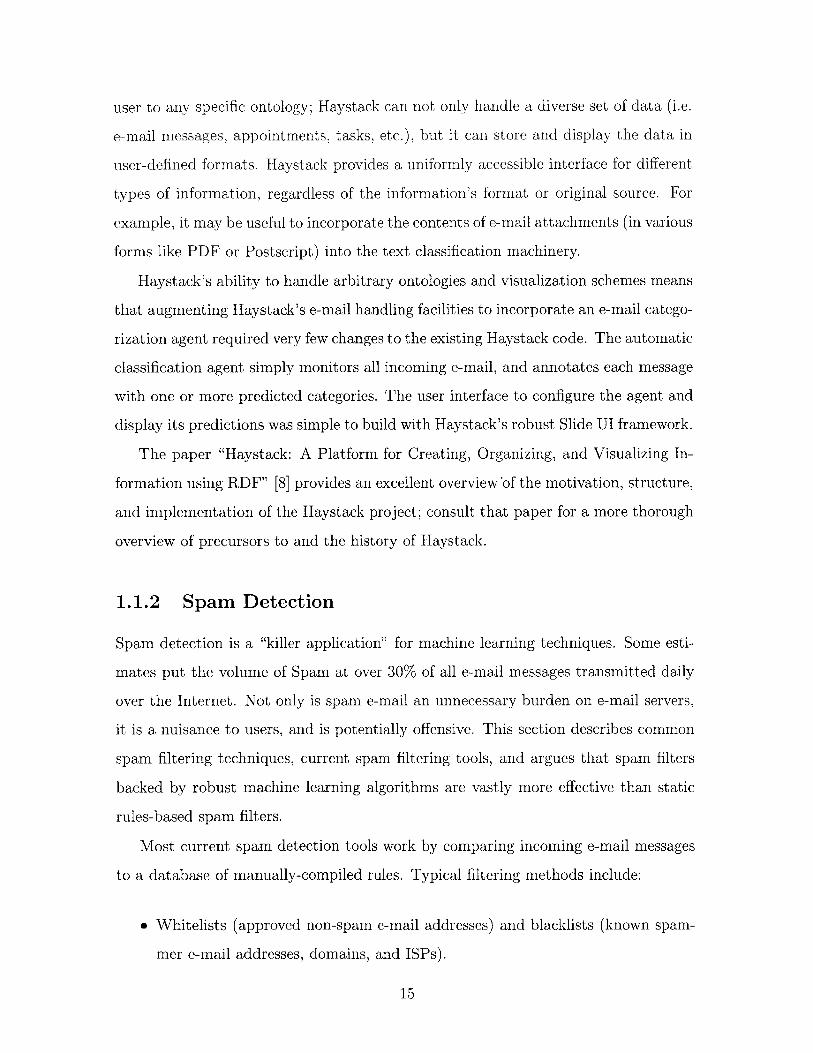
1.1.2 Spam Detection
Spam detection is a "killer application" for machine learning techniques. Some esti-
mates put the volume of Spam at over 30% of all e-mail messages transmitted daily
over the Internet. Not only is spam e-mail an unnecessary burden on e-mail servers,
it is a nuisance to users, and is potentially offensive. This section describes common
spain filtering techniques, current spam filtering tools, and argues that spam filters
backed by robust machine learning algorithms are vastly more effective than static
rules-based spain filters.
Most current spain detection tools work by comparing incoming e-mail messages
to a database of manually-compiled rules. Typical filtering methods include:
* Whitelists (approved non-spam e-mail addresses) and blacklists (known spam-
mer e-mail addresses, domains, and ISPs).
15

" The presence of anomalous e-mail message headers (forged senders, etc.) and
e-mail message headers that indicate that a message was generated by a bulk
e-mail sending program.
" Searching the message for certain pre-defined words, phrases, or types of text
(such as sentences in ALL CAPS).
The advantage of these types of e-mail filters is that they don't require any training
- they can immediately start filtering spam e-mail, even if there is very little initial
data (i.e. the user has only received a few e-mail messages). However, rules based
filters have no ability to adapt to a specific user's e-mail. For example, a sex education
worker might receive a high number of important work-related e-mails that have
common spam keywords in them. The adaptive nature of machine learning algorithms
makes them more powerful than rules based filtering for a number of reasons:
" Machine-learning algorithms can adapt to an individual's e-mail. People who
maintain rules-based filters for spam detection often include personal informa-
tion - such as their home telephone number or zip code - in their personal
set of spam rules [7]; personal information (other than your e-mail address and
perhaps your first name) is highly unlikely to be present in spam e-mail, and
is thus an excellent discriminator. While rules-based filters must be manually
programmed with personal information, machine learning algorithms will auto-
matically learn good discriminants.
" The "spam score" of a message computed by a rules-based filter is somewhat
arbitrary. Most rules-based filters work by assigning each characteristic of an
e-mail a spam score; if the score for a specific e-mail message exceeds a set limit,
then the message is classified as spam. How many points should an e-mail get
for having the word "sex" in it? A machine learning algorithm's logic is based
on empirical observation of its training corpus, not a human's guess.
* Static rules-based spam filters cannot adapt to changing patterns in e-mails.
Spam detection tools reduce the profitability of spam to its senders; spammers
16

will obviously try to look for ways around them. As rules-based filters have
become more widely deployed, some spammers have tried to evade simple word-
blocking spam filters by, for example, writing the word "porn" as "pOrn". Rules-
based filters must be updated to reflect changing trends in spam content, but
machine-learning algorithms can automatically adapt to changes in spam; they
might misclassify the first few messages, but as long as the user is diligent about
correcting the learner's mistakes, the new type of spam will quickly be caught.
In fact, a machine learning algorithm is likely to learn that the word "pOrn" is
an excellent discriminator between spam and legitimate e-mail - an ever better
discriminator than the word "porn".
Some spain researchers [6] predict that adaptive spam detection algorithms will
mean the death of spam. The only way spammers will be able to craft messages
that escape an adaptive spam filter is to make their messages indistinguishable from
your ordinary e-mail. Spam messages are mostly sales pitches, so unless your regular
e-mail is mostly sales pitches, it's unlikely that a majority of spain would get through
an adaptive spain filter. As text learning algorithms become better and better at
distinguishing spam sales pitches from the normal flow of e-mail, they predict that
the torrent of spam will slow to a trickle.
Static rules-based spam detection algorithms do have their place in a robust spam
solution; it's hard, for example, to get a machine learning algorithm to learn whether
an e-mail has a malformed header or not, but it's easy to write a rule to detect this.
Adaptive machine learning algorithms are powerful, but they aren't a panacea; the
best spam detection systems will most likely use static rules alongside state of the
art machine learning algorithms. The combination of the expressive power of static
rules and the adaptiveness of machine learning algorithms is sure to form the basis
of a very formidable spam detection solution.
1.2 Overview
This thesis is divided into six sections.
17

Chapter 2 discusses the design considerations involved in building a text classifica-
tion system. One important aspect of any text classification system is its document
representation scheme; most machine learning algorithms cannot process raw text
documents, and a document representation scheme defines how a text document is
presented to the machine learning algorithms. The most common document represen-
tation is a "bag-of-words" or "word frequency vector," which is simply a histogram
of the words in a given document. These word frequency vectors are computed by
Lucene, which was customized to efficiently store this data and is described in Chapter
3. Once all documents have been translated into word frequency vectors, a number of
pre-processing algorithms may be run. These pre-processing algorithms help remove
noise and clean the word frequency vectors before they are input into the machine
learning algorithms.
The machine learning algorithms are the backbone of the learning framework,
and are described in Chapter 4. Broadly, each algorithm takes as input a set of word
frequency vectors already labeled with categories, builds a model from this training
data, and then applies that model to the test data. The goal of the model is to
label new documents like "similar" already-labeled documents. The learning frame-
work supports three different types of classifiers: binary classifiers, which determine
if a document is in a class, multi-class classifiers, which label a test document with
exactly one class out of a possible field of many classes, and multi-label classifiers,
which label a test document with any number of labels. The framework provides
binary classifiers and multi-label classifiers that can handle fuzzy data. Java inter-
faces are used extensively, and similar classifiers can be swapped in and out with no
significant code modifications. The various classifiers implemented in this thesis have
been benchmarked using standard test corpora, and the algorithms perform on par
with published implementations.
The learning framework was used to build two applications: Cesium, an auto-
classification agent for Haystack, and PorkChop, a spam-filtering plugin for Microsoft
Outlook. Cesium is discussed in Chapter 5, and PorkChop is discussed in 6.
Finally, the Cholesterol database is the backend RDF store for the Haystack
18

project and is an integral part of Haystack. It is not directly related to the learning
framework, but I performed a significant amount of development work on Cholesterol.
Cholesterol is described in Chapter 7.
19

20

Chapter 2
How to Build a Text Classification
System
This section describes how to build a text classification system. As the name implies,
the goal of a text classification system is to process a document and label that doc-
ument as a member of one or more groups. A text classifier takes as input a set of
training documents, each labeled as a member of one or more groups, and tries to
learn a model from this training data. The specifics vary by algorithm, but classifica-
tion models, in general, try to identify which features of the training documents can
be used to separate the training documents among their assigned classes. Some learn-
ing algorithms can also handle fuzzy training data, where documents can be labeled
as "probably" a member of a category, or "definitely" not a member of a category,
and this uncertainty about training labels influences the classification model. Once
a model has been built from the training data, the classifier analyzes test documents
and uses the model to assign these documents labels.
However, a fully functional text classification system requires much more than
machine learning algorithms. This chapter provides an overview of all of the con-
stituent parts of an text classification system, with the exception of the specifics of
the machine learning algorithms, which are discussed in Chapter 4. Machine learn-
ing algorithms can't process raw text; text documents must first be converted into a
computer-friendly document representation. Section 2.1 discusses common document
21

5standardST ANDARD OIL SRD TO FORM FINANCIAL UNIT
Ij managementStandard Oil Co and BP North America plan to form a venture to manage 4 oilthe money market activities of both companies. BP North America is a -
subsidiary of British Petroleum Co Plc BP, which also owns a 55 pct
interest in Standard Oil.
The venture will be called BP/Standard Financial Tradinga and will under
be operated by Standard Oil under the oversight of a joint management H of
committee. venture
Figure 2-1: A word frequency vector
representations and how they shape the nature of the classification problem. Once a
text document has been converted into a computer-friendly representation, a number
of pre-processing algorithms can be run on the data. These pre-processing algorithms,
which are discussed in Section 2.2 "clean" the document representation by exploiting
properties of the English language to remove extraneous features, reduce noise, and
improve the ability of the classifier to generalize. Section 2.3 provides an overview of
the Java APIs provided by the Haystack Learning Framework to generate a computer-
friendly document representation from a text document and to pre-process a corpus
of documents.
Once the computer-friendly document representation has been cleaned via the
pre-processing algorithms, it is ready to be fed into the classifier. Chapter 4 provides
an in-depth discussion of the machine-learning algorithms implemented in this the-
sis; Section 2.4 discusses various high-level aspects of machine learning. Specifically,
Section 2.4 motivates the need for a fuzzy learning framework and addresses a num-
ber of practical issues one must take into consideration when designing a real-world
classifier.
Finally, Section 2.5 discusses various methodologies for evaluating the performance
of a classifier.
2.1 Document Representation
The simplest way to represent a text document is the "bag-of-words" or "word fre-
quency vector" representation. A word frequency vector is produced by tokenizing
a document using a tool like Lucene (Chapter 3), and building a histogram of the
22

"Some people like to eat dogs" "Some dogs like to eat people"
1 some
1 people
1 like
1 to
1 eat
1 dogs
Figure 2-2: Two semantically different sentences generate the same word vector
Document 1 Document 2 Document 1 Document 2
5 standard 1 merger 1 standard 5 merger
3 management 5 HP 3 management 5 HP
I oil 3 Compaq - 3 oil 1 Compaq
I under 4 Fiorina 4 under 1 Fiorina
2 listen 1 Hewlett 1 listen 2 Hewlett
Figure 2-3: An illustration of Rennie and Rifkin's experiment [17]
number of occurrences of each word in the document. It is relatively easy to compute
a word frequency vector from a text document, and these word vectors are convenient
to work with. However, any information about phrases within the document is lost.
At first approximation, it seems obvious that grouping relevant word pairs in the
vector representation will be useful to the classifier - "machine learning" is more
useful than "machine" and "learning." However, it's important to group the right
word pairs; grouping the phrases "the dog" and "a dog" may actually decrease the
accuracy of the classifier (both phrases refer to the same concept - a "dog"). It
is computationally infeasible to generically determine which word pairs it would be
advantageous to group without any higher order, domain specific information.
23

The Independence Assumption
Due to the intractability of determining which word pairs are relevant and which word
pairs are not relevant, most text classification systems impose a simplifying "inde-
pendence assumption", which states that each word in a document is independent of
all other words in the document. While it does seem logical that grouping word pairs
would be helpful to a classifier, a number of studies have borne out the independence
assumption. Rennie and Rifkin [18] found no improvement classifying two different
datasets with non-linear SVM kernels over linear SVM kernels, and Yang and Liu
[28] duplicated this result on the Reuters-21578 dataset. Furthermore, Rennie and
Rifkin have run experiments that show that randomly scrambling word frequencies
between documents yields a classifier with the same accuracy for a linear SVM (see
Figure 2-3) [17]. The independence assumption dramatically shapes the nature of
text classification algorithms.
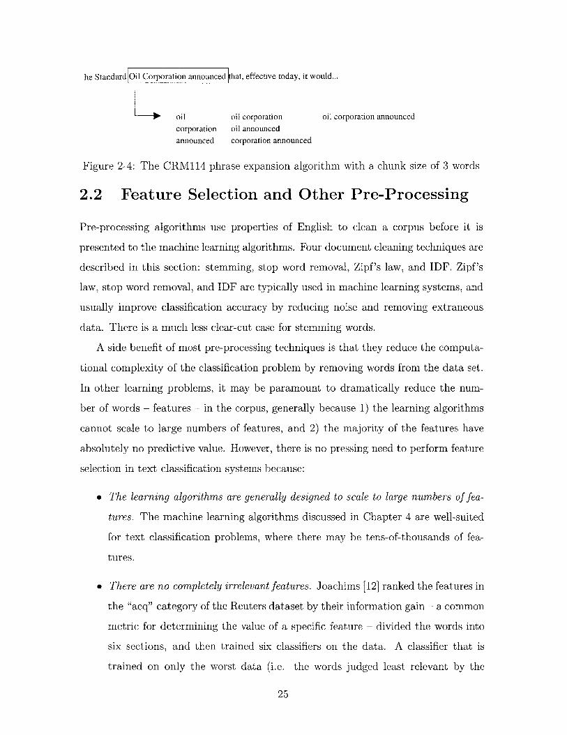
2.1.1 CRM114 Phrase Expansion Algorithm
The CRM114 spam filter (discussed in Section 6) is a spam filtering tool with a novel
approach to feature generation. While the general logic when designing machine
learning systems is to use as few features as possible (to reduce computation time
and to prevent overtraining), the CRM114 spam filter generates as many features as
possible from the document text.
CRM114 moves a 5-word sliding window over the document, and generates ev-
ery possible combination of subphrases for that 5-word window (see Figure 2-4).
The author has no solid theoretical background for reversing common practice, but
CRM114's impressive accuracy using a Naive Bayes classifier lends some credence to
his design decisions. While his work is preliminary, unverified, and not solidly the-
oretically founded, it's worth examining; a tokenizer that implements CRM114-style
phrase expansion algorithm is discussed in Section 2.3.1.
24
he Standard Oil Corporation announced that, effective today, it would...
oil oil corporation oil corporation announced
corporation oil announcedannounced corporation announced
Figure 2-4: The CRM114 phrase expansion algorithm with a chunk size of 3 words
2.2 Feature Selection and Other Pre-Processing
Pre-processing algorithms use properties of English to clean a corpus before it is
presented to the machine learning algorithms. Four document cleaning techniques are
described in this section: stemming, stop word removal, Zipf's law, and IDF. Zipf's
law, stop word removal, and IDF are typically used in machine learning systems, and
usually improve classification accuracy by reducing noise and removing extraneous
data. There is a much less clear-cut case for stemming words.
A side benefit of most pre-processing techniques is that they reduce the computa-
tional complexity of the classification problem by removing words from the data set.
In other learning problems, it may be paramount to dramatically reduce the num-
ber of words - features - in the corpus, generally because 1) the learning algorithms
cannot scale to large numbers of features, and 2) the majority of the features have
absolutely no predictive value. However, there is no pressing need to perform feature
selection in text classification systems because:
" The learning algorithms are generally designed to scale to large numbers of fea-
tures. The machine learning algorithms discussed in Chapter 4 are well-suited
for text classification problems, where there may be tens-of-thousands of fea-
tures.
* There are no completely irrelevant features. Joachims [12] ranked the features in
the "acq" category of the Reuters dataset by their information gain - a common
metric for determining the value of a specific feature - divided the words into
six sections, and then trained six classifiers on the data. A classifier that is
trained on only the worst data (i.e. the words judged least relevant by the
25

information gain metric) still performs significantly better than average. This
implies that it's good to have all of the features in the document; a good text
classifier should learn many features, and there are few completely irrelevant
features.
Most text classification systems still perform some form of pre-processing, but the
goal of the pre-processing is not to make the problem computationally tractable or to
eliminate irrelevant features; the pre-processing algorithms used in text classification
systems typically clean the data, reduce noise, and try to increase the ability of a
classifier to generalize.
The Haystack Learning Framework provides four different pre-processing methods.
2.2.1 Stop Word Removal
Stop word removal is an easy-to-implement pre-processing step that removes common
words that are known to contribute little to the semantic meaning of an English
document. Typical stop words include "the," "of," "is," etc. Lucene provides a
mechanism to remove stop words when tokenizing a document.
2.2.2 Zipf's law
Zipf's law says that the r-th most frequent word will occur, on average, 1 times the
frequency of the most frequent word in a corpus. This implies that most of the words
in the English language occur infrequently. Removing extremely rare words not only
reduces dimensionality, it also improves classifier accuracy; the logic is that rare words
might have excessive discriminatory value.
The default pre-processor in the Haystack Learning Framework removes any words
that occur only once or twice in the entire corpus.
2.2.3 Inverse Document Frequency
The inverse document frequency (IDF) algorithm is used to reduce the effect of com-
mon words on a classifier and increase the effect of uncommon words on the classifier.
26

The rationale is that common words have little discriminatory value, while relatively
uncommon words are more effective in separating document classes. Once a word
frequency vector has been computed for every document in the corpus, the IDF al-
gorithm can be applied to each document. The IDF formula is as follows:
IDF(Wi) = log (D ) (2.1)(DF(Wi)
IDj represents the total number of documents in the corpus, and DF(W) repre-
sents the number of documents word Wi is present in. It is intuitive from Equation
2.1 that the inverse document frequency of a word is low if it appears in many doc-
uments. The logic is that words that appear in a large percentage of documents are
of little value in discriminating between documents. While words that appear only
once or twice in the entire corpus are removed (in accordance with Zipf's law), the
inverse document frequency is highest when a word appears in fewer documents.
The IDF formula is applied to each document as follows:
dIDF = [Frequency(W1) * IDF(W), ... , Frequency(Wn) * IDF(Wn)] (2.2)
The weight of each word in a document (the number of times that word appears in
the document) is scaled by the IDF of that word in the entire corpus. Common words
like "is" and "the" may appear frequently in each document (i.e. their Frequency(W)
is large), but because they appear in many documents in the corpus, their IDF will
be low.
2.2.4 Stemming
Stemming normalizes semantically similar words by removing the suffixes of words -
i.e. "learning" becomes "learn" and "dogs" becomes "dog." Not only does stemming
reduce the dimensionality of the word vector, it increases the ability of the classifier
to generalize to different word forms. Lucene (Chapter 3) provides a Porter Word
27

Stemmer [15], which can optionally be used by clients of the Haystack Learning
Framework to normalize word forms.
Stemming isn't a panacea - even the best stemming algorithms will make mistakes.
For example, "number" will be translated by a Porter Stemmer to "numb." The
decision to use a stemming algorithm to pre-process document data is a trade-off
between generalizeability and specificity. If you use a stemmer, then most word forms
will be correctly normalized and your classifier will theoretically generalize better
when faced with new documents. However, one can argue that by not stemming
words, one allows the classifier to capture more detail; for example, "played" implies
past-tense, and is distinct from "play," which could be used to represent either present
or future tense.
Most text classification systems use IDF, stop words, and Zipf's law to pre-process
corpus data; stemming is not nearly as universally applied as the other pre-processing
algorithms, as there is evidence that using a stemming algorithm can reduce classifi-
cation accuracy [20].
2.3 Tokenization and Pre-Processing API
Machine learning algorithms generally expect their input to come in the form of a
word frequency vector - a histogram of word frequencies in a document. However,
training and test documents are generally provided as flat text; they must be tokenized
and assembled into word frequency vectors before they can be fed into the machine
learning algorithms. Lucene provides robust tokenization tools, which are wrapped
by the learning framework's ITokenizer interface.
Pre-processing and tokenization are discussed together because two useful pre-
processing tools - stemming and stop word removal - are most easily done during
document tokenization. Section 2.3.1 discusses the Tokenization API, and Section
2.3.2 discusses the document pre-processing API.
28

2.3.1 Tokenization API
The ITokenizer interface presents a generic interface to tokenization.
interface ITokenizer
String nexto;void closeo;
}
Three different tokenizers are provided:
SimpleTokenizer
class SimpleTokenizer implements ITokenizer
{SimpleTokenizer(Reader r);
}
The SimpleTokenizer performs only rudimentary lexical analysis - it converts all
words to lowercase.
AdvancedTokenizer
The AdvancedTokenizer tokenizer provides facilities for stop word removal and stem-
ming. The list of stop words to remove is supplied by Lucene, as is the Porter Stemmer
algorithm.
class AdvancedTokenizer implements ITokenizer
AdvancedTokenizer(Reader r /* bStopWords = true, bPorterStemmer = true */ );AdvancedTokenizer(Reader r, boolean bStopWords, boolean bPorterStemmer);
P
PhraseExpandingTokenizer
The PhraseExpandingTokenizer implements the CRM114 phrase expansion algorithm
described in Section 2.1.1.
The PhraseExpandingTokenizer uses another tokenizer (such as a SimpleTokenizer
or an AdvancedTokenizer) to parse the incoming document. The chunk parameter
29
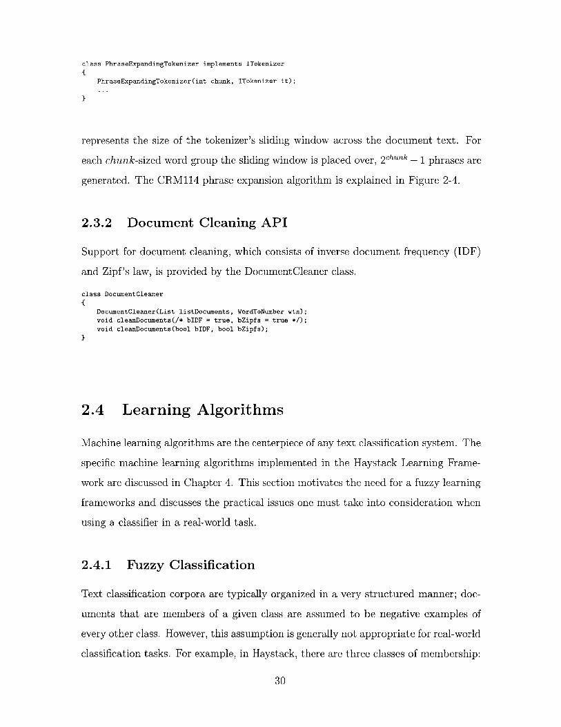
class PhraseExpandingTokenizer implements ITokenizer
{PhraseExpandingTokenizer(int chunk, ITokenizer it);
}
represents the size of the tokenizer's sliding window across the document text. For
each chunk-sized word group the sliding window is placed over, 2chunk - 1 phrases are
generated. The CRM114 phrase expansion algorithm is explained in Figure 2-4.
2.3.2 Document Cleaning API
Support for document cleaning, which consists of inverse document frequency (IDF)
and Zipf's law, is provided by the DocumentCleaner class.
class DocumentCleanerf
DocumentCleaner(List listDocuments, WordToNumber wtn);void cleanDocuments(/* bIDF = true, bZipfs = true */);
void cleanDocuments(bool bIDF, bool bZipfs);
}
2.4 Learning Algorithms
Machine learning algorithms are the centerpiece of any text classification system. The
specific machine learning algorithms implemented in the Haystack Learning Frame-
work are discussed in Chapter 4. This section motivates the need for a fuzzy learning
frameworks and discusses the practical issues one must take into consideration when
using a classifier in a real-world task.
2.4.1 Fuzzy Classification
Text classification corpora are typically organized in a very structured manner; doc-
uments that are members of a given class are assumed to be negative examples of
every other class. However, this assumption is generally not appropriate for real-world
classification tasks. For example, in Haystack, there are three classes of membership:
30

definite positive examples, definite negative examples, and possible negative exam-
ples. The learning framework provides support for "fuzzy" algorithms that allow
users to qualify a set of class labels with a confidence value.
Documents no longer have to be presented as strictly positive or negative exam-
ples; a document can be "definitely in class c" but "probably not in classes a and
2.4.2 Practical Training Issues
Training a classifier is a computationally intensive task. Depending on the classi-
fier used, training takes anywhere from 0(n) to 0(n2), where n is the number of
documents in the training corpus. The space requirements for training can also be
considerable; at best, the space requirements are O(ICI), where JCJ is the number of
classes, and at worst they are 0(n).
Research text classification systems are only run once; a document corpus is split
into a training and a test set, a classifier is trained on the training set, and then run on
the test set. Real-world text classification systems, on the other hand, must be able to
deal with a continuous stream of new documents, and they must be able to learn from
any classification mistakes. Both Cesium (Chapter 5), an automatic classification
system for Haystack, and PorkChop (Chapter 6), a spam filter for Microsoft Outlook,
constantly receive new documents and e-mail messages, and allow the user to correct
any mis-classifications.
Due to their internal workings, most classifiers cannot be trained incrementally -
i.e. the classifier must retrain on all documents in the training set to learn from even
one additional document. Because of the considerable time and space requirements
to train a classifier, it's not practical to retrain the classifier after each new mes-
sage. There are a number of schemes to reduce the frequency with which a learning
algorithm has to train:
" Scheduling. Schedule the classifier to retrain every 2-3 hours.
* Queue length. If there are more than, say, 25 documents in a "to be trained"
31

queue, then re-train the classifier.
e Train on errors. Train only when a classification error occurs.
The best training techniques may combine all three approaches. The goal is to
re-train the classifier frequently if the corpus is changing frequently or if the classifier
is inaccurate, and to reduce the training frequency in all other circumstances.
2.5 Evaluating Performance
The goal of this thesis is to develop a robust text classification system, not to break
new ground and develop a new learning algorithm. As such, the performance analysis
of the algorithms in this thesis is relatively unsophisticated. This section describes
the data sets and methodology used to analyze classifier performance; Section 4.4
discusses actual classifier performance.
Three data sets are used to evaluate performance:
" Reuters The Reuters data set is one of the most widely used data sets to
measure classifier performance. The data was collected by the Carnegie group
from the Reuters newswire in 1987, and was compiled by Lewis [13] into a corpus
of 21,450 articles that are classified into 135 topic categories. Each article can
have multiple category labels. 31% of all articles have no category labels (these
articles are not used), 57% of all articles are in exactly one category, and the
rest, 12%, have anywhere from one to twelve class labels. The distribution of
articles among the classes is very uneven.
" Personal Spam Corpus My personal spam corpus is derived from a collection
of personal e-mail and publicly available spam. It consists of 1,747 non-spam
e-mail messages and 1,613 spam e-mail messages, all from my personal Inbox.
" Twenty Newsgroups The Twenty Newsgroups data set is a collection 18,828
Usenet articles from twenty different newsgroups, with messages roughly evenly
32

distributed across each category. The original Twenty Newsgroups data set con-
tained exactly 20,000 articles, but Rennie has removed 1169 duplicate (cross-
posted) articles. The classifier attempts to predict which newsgroup a message
belongs in. Because each message is a member of exactly one newsgroup, the
Twenty Newsgroups data set is ideal for testing multi-class classification algo-
rithms.
All tests are performed using the same basic methodology:
* All documents are pre-processed by removing stop words, removing any words
that occur only once or twice in the entire corpus, and using the Inverse Docu-
ment Frequency (IDF) algorithm.
" Documents are randomly assigned to training or test sets. There are roughly
equal numbers of documents in the training and test sets. The training and
test splits are random, but documents are consistently assigned to either the
training or test set across multiple runs of the classifier. Some corpora, such
as Reuters, have standard, pre-defined training and test data splits, but these
pre-defined splits are ignored.
The learning framework implements three types of classification algorithms, and
each is tested differently:
2.5.1 Binary Classifiers
A binary classifier determines whether a document is in a class. Binary classifiers are
tested using the Spam Corpus and selected categories of the Reuters corpus.
Joachims [10] suggests using the "acq" and "wheat" categories of the Reuters
dataset to test classifiers. The "acq" category is the second most popular category,
and contains articles that discuss corporate acquisitions. The "wheat" category, on
the other hand, has relatively few news articles and concerns a very specific topic. A
simple classifier that assigns a document to the "wheat" category by searching for the
word wheat is 99.7% accurate. The "acq" category has no such characteristic word
33

or words; it represents a more abstract concept, and a successful classifier will have
to form a more complex model.
To evaluate the performance of a binary classifier, we collect the following data:
" The number of true positives. A true positive occurs when the classifier predicts
TRUE and the actual value is TRUE.
" The number of false positives. A false positive occurs when the classifier predicts
TRUE, but the actual value is FALSE.
" The number of false negatives. A false negative occurs when the classifier pre-
dicts FALSE, but the actual value is TRUE.
" The number of true negatives. A true negative occurs when the classifier predicts
FALSE and the actual value is FALSE.
We can represent this data in the following table:
Actual TRUE Actual FALSE
Classified Positive True Positive (TP) False Positive (FP)
Classified Negative False Negative(FN) True Negative (TN)
From this data, we can compute a number of statistics:
Statistic Equation
Correct predictions TP + TN
Incorrect predictions FN + FP
Sensitivity TP
Specificity FP+TN
The number of correct predictions is the most easily understood and commonly
referenced performance metric, and it generally gives a good picture of classifier per-
formance. However, if the test documents are unevenly distributed between classes,
then the sensitivity and specificity metrics are useful. For example, in the Reuters
test set, there are only 124 positive examples of documents in the "wheat" category
34

out of a total number of 5,041 documents in the test set. A classifier that always pre-
dicts that a document is not in "wheat" will achieve a 99.97% classification accuracy,
but will have a specificity of 0.
2.5.2 Multi-class Classifiers
A multi-class classifier assigns a document exactly one class label. Multi-class classi-
fiers are tested exclusively using the Twenty Newsgroups corpus.
To evaluate the performance of a multi-class classifier, we simply record the num-
ber of correct predictions.
2.5.3 Multi-label Classifiers
Multi-label classifier are generally constructed by using n binary classifiers - one for
each category. The performance of a multi-label classifier is entirely dependent on
the performance of the underlying binary classifiers.
35

36

Chapter 3
Forward Indexes and Lucene
3.1 Introduction
Lucene [16] is a fast, full-featured text search and indexing engine written in Java.
It uses disk-based indexes for high performance and low memory utilization, and
supports ranked searching, complex queries (such as boolean and phrase searches),
and fielded searching. Lucene is currently used to store an index of all text content
in Haystack, and to allow users to search that content.
A search engine like Lucene computes an inverted index - an index that is designed
to support efficient retrieval of all of the documents that contain a given search term.
An inverted index contains an entry for each word in the corpus; in this entry is a
Inverted Index
haystack Doc 1 3x, Doc 2 3x
ontology Doc 1 7x
pig Doc 4x, Doc 2 2x, Doc 3 6x
cholesterol Doc 1 2x, Doc 3 4x
farmer Doc 2 9x
cow Doc 2 4x
stress Doc 3 3x
cardiology Doc 3 Ix
Figure 3-1: An example of an inverted index
37
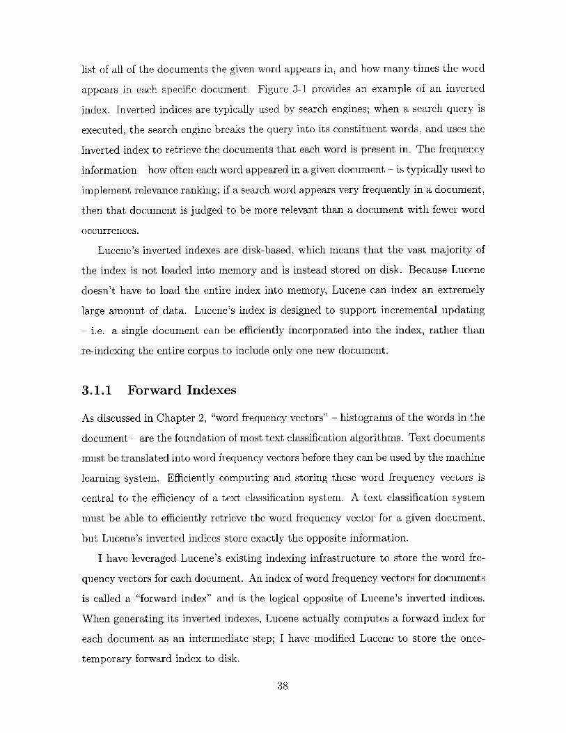
list of all of the documents the given word appears in, and how many times the word
appears in each specific document. Figure 3-1 provides an example of an inverted
index. Inverted indices are typically used by search engines; when a search query is
executed, the search engine breaks the query into its constituent words, and uses the
inverted index to retrieve the documents that each word is present in. The frequency
information - how often each word appeared in a given document - is typically used to
implement relevance ranking; if a search word appears very frequently in a document,
then that document is judged to be more relevant than a document with fewer word
occurrences.
Lucene's inverted indexes are disk-based, which means that the vast majority of
the index is not loaded into memory and is instead stored on disk. Because Lucene
doesn't have to load the entire index into memory, Lucene can index an extremely
large amount of data. Lucene's index is designed to support incremental updating
- i.e. a single document can be efficiently incorporated into the index, rather than
re-indexing the entire corpus to include only one new document.
3.1.1 Forward Indexes
As discussed in Chapter 2, "word frequency vectors" - histograms of the words in the
document - are the foundation of most text classification algorithms. Text documents
must be translated into word frequency vectors before they can be used by the machine
learning system. Efficiently computing and storing these word frequency vectors is
central to the efficiency of a text classification system. A text classification system
must be able to efficiently retrieve the word frequency vector for a given document,
but Lucene's inverted indices store exactly the opposite information.
I have leveraged Lucene's existing indexing infrastructure to store the word fre-
quency vectors for each document. An index of word frequency vectors for documents
is called a "forward index" and is the logical opposite of Lucene's inverted indices.
When generating its inverted indexes, Lucene actually computes a forward index for
each document as an intermediate step; I have modified Lucene to store the once-
temporary forward index to disk.
38

Forward Index
Document I Document 2 Document 3
3 haystack 9 farmer 3 stress
7 ontology 4 cow 6 pig
4 pig 2 pig 4 cholesterol
2 cholesterol 3 haystack 1 cardiology
Figure 3-2: An example of a forward index
3.2 The Modifications to Lucene
The standard Lucene distribution does not provide an efficient means of accessing
the attributes of a specific document. I have modified Lucene to support efficient
retrieval of a document's word frequency vector using a unique ID.
When a client adds a document to Lucene, he can specify one or more fields;
typical fields might include "author," "subject," or "text." To retrieve a document
via a unique ID, the unique ID must be specified in a document field. Specifically,
the user must place the document's unique ID in its own field, and this field - termed
the "primary field" in the rest of this chapter - is specially recognized by my Lucene
modifications. I have added accessors that make retrieving a document by its primary
field as easy as calling one method in Lucene's IndexReader class.
It's possible to retrieve a document by constructing a search object, restricting
the search space to the primary field, and then searching for a document's unique
ID. The desired document should be the first and only entry in the search results.
However, looking a document up by its unique ID is a common operation for any user
of the new forward indexes, and the aforementioned process involves quite a bit of
code. IndexReader's accessor methods wrap this complexity and make retrieving a
document by its unique ID a one-step operation.
Lucene's new index format is backwards-compatible with the old Lucene index
format - users of other versions of Lucene can access indexes created by the forward-
39

index generating Lucene - and there is no performance impact on users of the modified
Lucene library who only create an inverted index. Existing Lucene code will compile
and run without modification if combined with the new Lucene library.
Like Lucene's inverted indexes, the forward indexes are disk-based and can be
incrementally updated.
3.2.1 API
Lucene's interfaces are little-changed from the standard distribution. Lucene in-
dexes are typically created via the IndexWriter class; I have created a new class,
ForwardIndexWriter, that is a subclass of IndexWriter. The only public difference
between ForwardIndexWriter and IndexWriter is the ForwardIndexWriter construc-
tor, which takes a "primary field" argument. The primary field contains a document's
unique ID; when documents are added to the forward index, they must store the doc-
ument's unique ID in the primary field.
class ForwardIndexWriter extends IndexWriter
ForwardIndexWriter(String primaryField, ... );
}
Figure 3-3: The ForwardIndexWriter class
IndexWriter iw = new ForwardIndexWriter("URI", ... );
Document d = new Documento;d.add(Field.Keyword("URI", "<urn:chrPQygXbyyAlupt>"));
d.add(Field.Text("text", strDocumentText));
iw. addDocument (d);
iw.closeo;
Figure 3-4: Adding a document to a forward index. The name of the document'sprimary field is "URI," and the contents of that field are the document's URI.
Documents can have multiple fields, and the data stored in each field is kept
separate from the data stored in other fields. Lucene's fields allow search engines to
implement relevance ranking algorithms; i.e. if a search term occurs in the subject of
a document, it can be judged more relevant than if the search term had only occurred
in the body of the document.
40
I use Lucene's fields to uniquely identify documents. The "primary field" specified
in the ForwardIndexWriter constructor must be specified by each document, and must
contain that document's unique ID. It is added to each document during indexing
via the Document class's add method. When adding fields to a document, users can
add the field using Field.Text, which performs tokenization on the specified text,
or Field.Keyword, which does not perform any tokenization. Users must add the
primary field to the document using Field.Keyword; a runtime exception will occur
upon document retrieval if the document's unique ID contains more than one token.
Field.Text should be used for regular text fields.
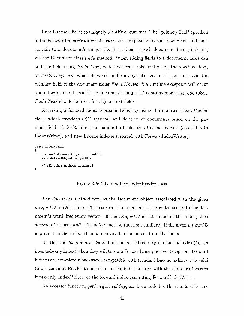
Accessing a forward index is accomplished by using the updated IndexReader
class, which provides 0(1) retrieval and deletion of documents based on the pri-
mary field. IndexReaders can handle both old-style Lucene indexes (created with
IndexWriter), and new Lucene indexes (created with ForwardlndexWriter).
class IndexReader
{Document document(Object uniqueID);
void delete(Object uniqueID);
// all other methods unchanged
}
Figure 3-5: The modified IndexReader class
The document method returns the Document object associated with the given
uniquelD in 0(1) time. The returned Document object provides access to the doc-
ument's word frequency vector. If the uniqueID is not found in the index, then
document returns null. The delete method functions similarly; if the given uniquelD
is present in the index, then it removes that document from the index.
If either the document or delete function is used on a regular Lucene index (i.e. an
inverted-only index), then they will throw a ForwardUnsupportedException. Forward
indices are completely backwards compatible with standard Lucene indexes; it is valid
to use an IndexReader to access a Lucene index created with the standard inverted
index-only IndexWriter, or the forward-index generating ForwardIndexWriter.
An accessor function, getFrequencyMap, has been added to the standard Lucene
41

Document class:
class Document {public FrequencyMap getFrequencyMapO;
// all other methods unchanged
}
Figure 3-6: The modified Document class
Document objects can be returned from a number of IndexReader methods. If the
IndexReader that returned the Document class is accessing a forward index, then the
getFrequencyMap function will return a FrequencyMap class, which provides easy
access to the word frequency vector for a given document (see Section 2.1 and Figure
2-1 for an explanation of word frequency vectors). Otherwise, if the IndexReader is
accessing an old-style Lucene index, then the getFrequencyMap function will return
null.
42

Chapter 4
The Haystack Learning Framework
The Haystack Learning Framework module provides a robust text-learning framework
with implementations of binary classifiers, multi-class classifiers, and multi-label clas-
sifiers. The Learning Framework provides two binary classification algorithms, Reg-
ularized Least Squares Classification (RLSC) and Naive Bayes, four multi-class clas-
sification algorithms, Rocchio, Error Correcting Output Codes (ECOC), Multi-class
Naive Bayes, and One vs. All, and one multi-label classification algorithm, Simple
Multi-Label.
Three interfaces, IBinaryClassifier, IMultiClassClassifier, and IMultiLabelClassi-
fier, correspond to the three types of classifiers offered by the Learning Framework.
The liberal use of interfaces allows users to swap-in different learning algorithms with
little or no change to the client code.
4.1 Types of Classification Problems
The goal of a text classification algorithm is to assign a document a label based upon
its contents. There are several different types of classification problems.
* Binary Classification: the classifier labels each document as positive or negative.
Many powerful classifiers (Support Vector Machines, RLSC) are natively binary
classifiers.
43

" Multi-class Classification: the classifier assigns exactly one of JC labels to a
document. Some algorithms are natively multi-class (i.e. Rocchio), while other
algorithms build upon binary classifiers.
" Multi-label Classification: the classifier assigns 0 to JCJ labels to the document.
This type of classification best meshes with Haystack's flexible categorization
scheme.
4.2 Binary Classification
A binary classifier takes as input a set of documents, where each document is labeled
either TRUE or FALSE. The binary classifier then trains on these documents. A new
test document is presented as input, and the classifier returns a TRUE or FALSE
label.
Haystack implements two binary classification algorithms: Regularized Least Squares
Classification and Naive Bayes.
4.2.1 API
Haystack provides a drop-in interface for binary classification via the IBinaryClassi-
fier interface. Two binary classification algorithms are provided: Regularized Least
Squares Classification and Naive Bayes. All binary classifiers implement the IBina-
ryClassifier interface (see figure 4-1).
interface IBinaryClassif ier
void addDocument(IDocumentFrequencyIndex dfi, boolean bClass);void traino);double classify(IDocumentFrequencyIndex dfi);
}
Figure 4-1: The IBinaryClassifier interface
* addDocument The addDocument method adds a document to the binary clas-
sifier. It takes two arguments: a word frequency vector representation of the
document to add, and a boolean that indicates the document's class.
44
" train The train method trains the classifier. You cannot call addDocument after
calling train, and you cannot call classify before calling train.
" classify The classify method applies the learned classifier to a test document.
It takes one argument - a word frequency vector - and returns a floating point
number. All binary classifiers center their classifier's return values around 0.0.
If the floating point number returned by classify is greater than 0.0, then a
document is generally labeled TRUE; otherwise, a document is labeled FALSE.
The magnitude of the return value implies the classifier's degree of confidence
in its prediction.
However, the significance of the magnitude is dependent on the specific classifier.
A classifier like RLSC generally places negative documents close to -1, and
positive documents close to 1, while the values returned by Naive Bayes vary
depending on the internal classifier state. Users of the binary classifier are
free to interpret its return values however they like; by adjusting the decision
threshold from 0.0, one can decrease the number of false positives at the expense
of increasing false negatives, or vice versa.
Binary classifiers are given a loose specification for handling boundary conditions;
their answers in boundary cases may not make sense, but the classifier must return a
value (i.e. it must not crash). If Naive Bayes or RLSC is trained on a corpus where
all documents are in one class, then they will predict that every document is in that
class. If either binary classifier is trained on a corpus with no training documents,
then its classify method will return an ambiguous answer of 0.0.
Fuzzy Binary Classification
Machine learning problems are typically well defined - a document is either a positive
or negative example of a class - but real-world problems are rarely as clearly defined.
A document might be "probably true" or perhaps "definitely false," and traditional
binary classifiers do not model this distinction. The binary classification algorithms
in this section are tailored towards "fuzzy" classification problems. Every training
45

document is accompanied by a confidence value that indicates the probability that
the training document's label is correct.
All fuzzy binary classifiers must implement IFuzzyBinaryClassifier.
interface IFuzzyBinaryClassifier{
void addDocument(IDocumentFrequencyIndex dfi, boolean bClass, double dConfidence);void trainO;double classify(IDocumentFrequencyIndex dfi);
}
Figure 4-2: The IFuzzyBinaryClassifier interface
" addDocument The addDocument method adds a document to the binary clas-
sifier. It takes three arguments: a word frequency vector representation of the
document to add, a boolean that indicates the document's class, and a confi-
dence value. The confidence value is a floating point number from 0.0 to 1.0
that quantifies how confident the user is in the document's class label; a 1.0
confidence value implies absolute certainty, and values close to 0.0 imply a large
degree of uncertainty. Due to internal implementation details, documents with
very small confidence values - less than 0.0001 - are ignored.
" train The fuzzy train method functions identically to the traditional classify
method.
" classify The fuzzy classify method functions identically to the traditional classify
method.
The learning framework provides fuzzy implementations of both Naive Bayes and
RLSC.
4.2.2 Naive Bayes
Naive Bayes is a relatively simple text classification model that is often utilized in text
classification. Naive Bayesian classifiers run in linear time and achieve remarkable
performance; Naive Bayes is generally considered to be the best linear-time classifier
46

available. Naive Bayes can be used both as a binary and a multi-class classifier,
but the mathematical formulations for both types of classifiers are the same and are
discussed in this section.
A Naive Bayes classifier is predicated upon the fact that all attributes of the
training examples are conditionally independent - i.e. all words are independent of
each other given the context of their class. This assumption is known as the "Naive
Bayes assumption," and while it is clearly false, Naive Bayes classifiers perform well
in most real-world tasks. Because of the Naive Bayes assumption, features can be
learned separately, which greatly simplifies learning, especially when there are a large
number of attributes.
The Haystack Learning Framework uses the multinomial event model. Other
models exist, and all models have been referred to in the literature as "Naive Bayes,"
which causes some confusion. McCallum and Nigam [14] give a good overview of the
difference between the competing event models, and show conclusively that multino-
mial Naive Bayes is superior to other formulations.
A multinomial Naive Bayes classifier classifies a test document T by computing
the probability that T is in each of the potential document classes. The probability
for each individual class is determined by computing the probability that the words
in the test document T would appear in a document of that class.
To train, a Naive Bayes classifier computes P(wtlcj) for each word in the corpus
vocabulary, V, where IVI represents the total size of the corpus vocabulary, IDcj I rep-
resents the total number of words in document class cj, and weight(wi, cj) represents
the frequency with which word wi occurs in cj:
1 +El weight(wj, cj)P(wIcj) = + w t + (4.1)
A document is classified by computing
argmaxc P(cjjdt) (4.2)
where
47
P (cjIdt) - P(cj )P(dtlcj) (43)P(dt)
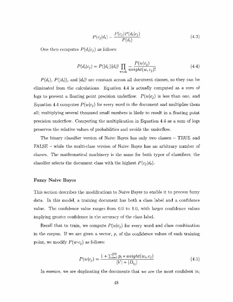
One then computes P(dtlcj) as follows:
P(dtlcj) = P(dtj)dtj! P(wc) (4.4)wEdt weight(w, ci)
P(dt), P(ldtl), and Idtl! are constant across all document classes, so they can be
eliminated from the calculations. Equation 4.4 is actually computed as a sum of
logs to prevent a floating point precision underflow. P(wlcj) is less than one, and
Equation 4.4 computes P(wlcj) for every word in the document and multiplies them
all; multiplying several thousand small numbers is likely to result in a floating point
precision underflow. Computing the multiplication in Equation 4.4 as a sum of logs
preserves the relative values of probabilities and avoids the underflow.
The binary classifier version of Naive Bayes has only two classes - TRUE and
FALSE - while the multi-class version of Naive Bayes has an arbitrary number of
classes. The mathematical machinery is the same for both types of classifiers; the
classifier selects the document class with the highest P(cj Idt).
Fuzzy Naive Bayes
This section describes the modifications to Naive Bayes to enable it to process fuzzy
data. In this model, a training document has both a class label and a confidence
value. The confidence value ranges from 0.0 to 1.0, with larger confidence values
implying greater confidence in the accuracy of the class label.
Recall that to train, we compute P(wlcj) for every word and class combination
in the corpus. If we are given a vector, p, of the confidence values of each training
point, we modify P(wlcj) as follows:
P(wlc ) = 1 + Z =1 PZ * weight(wi, cj) (4.5)IVI + DC|
In essence, we are duplicating the documents that we are the most confident in;
48

the weights of a document with a confidence value of 1.0 are twice the weights of a
document with a confidence value of 0.5.
4.2.3 Regularized Least Squares Classification
Regularized Least Squares Classification is a new method described by Ryan Rifkin
in his PhD thesis [19]. It is by no means a new algorithm [3, 1], but Rifkin's thesis is
the most comprehensive exploration of the problem to date. RLSC provides similar
classification accuracy to Support Vector Machines, but requires less time to train.
The exact time required to train a RLSC classifier (or a SVM), is a complex topic
with many variables and is discussed further in Rifkin's thesis; we'll simply have to
take his word that RLSC can be trained faster than a SVM.
RLSC and SVM's belong to a general class of problems called Tikhonov regular-
ization problems. While a thorough discussion of the mathematics behind Tikhonov
regularization problems is beyond the scope of this thesis, the concept is simple. A
Tikhonov regularization problem tries to derive a function, f, that accurately predicts
an answer, y, given an input x. The accuracy of f is measured using a loss function,
V(yi, f(xi)), and one attempts to find the f that minimizes the total loss. We can
state this formally as follows:
min - V(yi, f (xi)) + A l If|I 1 (4.6)
In the case of text classification, yj represents the binary label of a training case xi,
and f is the decision function that we're trying to derive. The norm expression I f I'
and the A parameter quantify our willingness to trade off training set error for the
risk of overtraining. A Tikhonov regularization problem can be used to describe both
Regularized Least Squares Classification and Support Vector Machines; by using the
hinge loss function V(f(x, y)) = (1 - yf(x)))+, one can re-derive a Support Vector
Machine (Chapter 2 of Rifkin's thesis). Replacing the hinge loss function with the
square loss function, V(f(x, y)) = (y - f(x)) 2 , Rifkin arrives at his Regularized Least
Squares algorithm. Because the square loss function is differentiable everywhere, the
49

mathematics for RLSC are much simpler than the mathematics for Support Vector
Machines. Substituting the square loss function in to Equation 4.6, the problem
becomes:
min - Z(y - f (i)) 2 + A 2fHj (4.7)fG7- f i=1
The goal of our classifier is to arrive at a decision function, f, that classifies a
training set with minimum error. Using the Representer Theorem, which is described
in Rifkin's thesis and [22], one can show that the decision function, f*, must take the
form:
f*(x) = ZciK(x, xi) (4.8)i=1
K represents a kernel matrix which is derived from the training data (its derivation
will be explained later). After we substitute Equation 4.8 into Equation 4.7 and
convert to matrix notation, we arrive at:
min (y - Kc)T(y - Kc) + AcTKc (4.9)CER
Now that the decision function, f, has a well-defined form, the problem begins
to take shape. In the above equation, f represents the number of documents, K is a
kernel function that is derived from the training data in an as-yet-undefined manner,
and y represents the true values of the training examples. c is a f dimensional vector
of coefficients for the decision function; to properly train our classifier, we must try to
find the c that minimizes the training error. Because RLSC uses a square loss function,
which is differentiable everywhere, and the kernel matrix K positive definite, we can
minimize Equation 4.9 by differentiating it and setting the equation equal to zero.
After differentiation and simplification, we find that the optimal c vector can be found
by solving the following equation:
(K + A )c = y (4.10)
50

In the above equation, I denotes an appropriately sized identity matrix, f is the
number of training documents, and A is a regularization parameter that quantifies
how willing we are to increase training set error but decrease the risk of overtraining.
A Tikhonov regularization problem requires an f x f kernel matrix K. However,
our training data is provided in an f x w matrix A that corresponds to the training
text (there are f rows, one for each document, and w columns, one for each unique
word). Because text classification is typically assumed to be a linear problem (see
Section 2.1), we can use a linear kernel K, which we compute simply by K = AAT.
Thus training our RLSC classifier becomes:
(AAT + AfJ)c = y (4.11)
Because (AAT + AfI) is positive definite and therefore invertible, a straightforward
way to solve this problem is to compute:
c = (AAT + AfI)-ly (4.12)
Unfortunately, solving this equation directly using a method like Gaussian elimi-
nation is intractable for large matrices. Methods like Conjugate Gradient (discussed
in Section 4.2.3) can solve this equation efficiently.
Once we have solved Equation 4.11 and discovered the appropriate c constants,
we have all parameters of our decision function, f. Recall from Equation 4.8 that
decision function, f, takes the following form:
f (x) = ZciK(x, xi) (4.13)i=1
Because the kernel, K, is linear and K = AAT, we can simplify the above equation
to:
f (x) = (cA T )x (4.14)
To classify a new data point, x, we compute (cA') and multiply by x.
51

Fuzzy RLSC
This section describes the necessary modifications to RLSC to enable it to handle
fuzzy data. In this model, a training document has both a class label and a confidence
value. The confidence value ranges from 0.0 to 1.0, with larger confidence values
implying greater confidence in the accuracy of the class label.
Equation 4.7 presents the RLSC minimization problem. Recall that the goal of
RLSC is to determine a function f that minimizes error, where the error is quantified
by summing (yi - f(xi))2 over a training corpus. Given an array of confidence values
p for each document, we can modify RLSC as follows:
I fmin - pi(yi - f (xi))2 + Aml If I1 (4.15)
The loss associated with a specific training document is multiplied by the confi-
dence value for that document, pi. If we minimize the above equation by differenti-
ating and simplifying, we arrive at:
(AAT + diag(p-1)XCI)c = y (4.16)
It is easy to see why the IFuzzyBinaryClassifier interface specifies that all doc-
uments with a confidence value of less than 0.0001 are ignored; dividing the right
side of the sum with a very small confidence value will result in a very large number,
which might cause in a floating point overflow.
Conjugate Gradient
The Conjugate Gradient method is an efficient means of computing the solution to
systems of linear equations of the form Ax = b. Conjugate Gradient is an iterative
algorithm; it begins with a candidate solution x', and iteratively refines the solution
until Ax' approaches b. The number of iterations required to converge on a specific
solution is variable and depends on A and b, though conjugate gradient generally
converges very quickly. Traditional algorithms like Gaussian elimination run in a
fixed amount of time, and operate directly on the matrix A.
52

Iterative algorithms like conjugate gradient are well-suited for problems such as
text classification, which involve large, sparse matrices. In a typical text classification
problem, A has anywhere from several hundred to several thousand rows (one for each
training document), and tens of thousands of columns (one for each distinct word in
the corpus), though only several hundred of the columns in each row will be non-zero.
It is easy to compute Ax' if A is a sparse matrix. Gaussian elimination, on the other
hand, performs row operations, which are exceedingly slow on large, sparse matrices.
Jonathan Richard Shewchuk's paper "An Introduction to the Conjugate Gradi-
ent Method Without the Agonizing Pain" [23] is an excellent introduction to the
conjugate gradient method.
4.2.4 Alternative Binary Classification Algorithms
Support Vector Machines
Support Vector Machines are currently regarded as the most capable binary classifi-
cation algorithm available. Broadly speaking, a SVM attempts to find a hyperplane
that maximizes the margin between positive and negative training examples, while
simultaneously minimizing training set misclassifications. SVMs are universal learn-
ers; by plugging in the appropriate kernel function, SVMs can learn linear threshold
functions, polynomial classifiers, radial basic function networks, and three-layered
sigmoid neural networks [11].
While SVMs are powerful, they do require approximately O(n 2) time to train
(Joachims [11] estimates between 0(n 7 ) and O(n 2 -)). This makes them infeasible
for large datasets (i.e. a million data points). The quadratic running time of Support
Vector Machines is their major downfall, and there have been a number of attempts
to overcome this problem:
o Subsampling: Subsampling involves training on only a subset of the total train-
ing data. By removing data from the training set, one loses a lot of information
and classifier performance suffers [17].
53

* Bundled SVM: A bundled SVM [24] reduces the number of training points
presented to a SVM learner by concatenating randomly chosen datapoints in the
same class. By tuning a s parameter that determines how many data points to
combine, one can achieve a tradeoff between accuracy and speed (between 0(n)
and the typical SVM 0(n2 )). The bundled SVM implementation described in
[24] achieves the current record for a ROC breakeven point on Reuters-21578,
though there is little theoretical justification for this result. Bundled SVMs
show a good deal of promise; even when the s parameter is tuned so the bundled
SVM runs in 0(n), the bundled SVM implementation still performs significantly
better than a benchmark Naive Bayes implementation.
Other Algorithms
* Neural Networks: A neural network is a type of classification algorithm pat-
terned off the physical neurons in brains. The network consists of groups of
nodes connected together in various patterns, with adaptive weights associated
with each connection. By varying the pattern of the nodes and adjusting the
function applied by the nodes, one can construct both linear and nonlinear
classifiers. Neural networks are generally slow to train, theoretically inelegant
(i.e. there are more direct ways to express a nonlinear classifier), and perform
relatively poorly [28].
" k-Nearest Neighbors: The k-Nearest Neighbor algorithm is simple in concept;
given a test document, the system finds the k-nearest neighbors to the document
according to a similarity measure (generally the same cosine metric used in the
Rocchio algorithm - see Equation 4.21). The neighbors are grouped according
to their category, and weighted according to their similarity scores. Training
a k-Nearest Neighbor classifier is simple (just record each document in the
training set), but given a m document training set and an n document test set,
classification takes 0(mn) time.
54
4.3 Multi-class and Multi-Label Classification Al-
gorithms
There are three broad types of classification algorithms: binary classifiers, multi-label
classifiers, and multi-class classifiers. Binary classifiers have been discussed already
in Section 4.2. Multi-label classifiers can assign a document 0 to ICI document labels,
while multi-class classifiers assign a document exactly one label.
This section describes four multi-class algorithms - One vs. All, Error Correcting
Output Codes (ECOC), Naive Bayes, and Rocchio - and one multi-label algorithm -
Simple Multi-Label. One can group these algorithms into two categories:
" Naturally multi-label or multi-class classifiers.
" Composite classifiers that build upon binary classifiers and decompose the clas-
sification task into any number of binary problems.
Algorithms like Rocchio and Naive Bayes are naturally multi-class, though both
can be used as binary classification algorithms. A binary classifier version of Naive
Bayes is described in Section 4.2.2. While Rocchio can also be converted to a binary
classifier, Joachims [10] has shown conclusively that Naive Bayes performs better than
Rocchio; Rocchio was not converted to be a binary classifier.
The most sophisticated algorithms - Support Vector Machines and RLSC - are
natively binary classifiers. While there has been some research regarding adapting
SVM and RLSC to be natively multi-class, the best results have been achieved by
combining binary classifiers to form a multi-class classifier [19]. Algorithms like Simple
Multi-Label, One vs. All, and Error Correcting Output Codes construct multi-class
or multi-label classifiers from arbitrary binary classifiers.
The learning architecture provides five multi-class or multi-label classification al-
gorithms:
* Simple Multi-Label. The simple multi-label algorithm trains ICI different binary
classifiers. To classify a document, the algorithm iterates through the ICI binary
classifiers; those that return TRUE are labeled with that class.
55

" Error Correcting Output Codes. Error Correcting Output Codes split the train-
ing data among 0(1 Cl) classifiers in a pattern that provides some error-correcting
properties.
" One vs. All. The One vs. All algorithm is a multi-class adaptation of the
Simple Multi-Label algorithm. It can be expressed via the matrix framework
used by ECOC classifiers.
" Naive Bayes. Naive Bayes is a popular and powerful linear-time inherently
multi-class classification algorithm.
" Rocchio. Rocchio is a natively multi-class algorithm that was implemented pri-
marily for debugging purposes. Naive Bayes is also linear-time and consistently
outperforms Rocchio.
4.3.1 API
Multi-Label Classification
The learning framework provides simple interfaces to multi-label and multi-class clas-
sification. A multi-label classifier must implement the IMultiLabelClassifier interface.
interface IMultiLabelClassifier
void addDocument(IDocumentFrequencyIndex dfi, Set classes);
void trainO;Set classify(IDocumentFrequencyIndex dfi);
}
Figure 4-3: The IMultiLabelClassifier interface
The SimpleMultiLabelClassifier is currently the only multi-label classifier imple-
mented in the Haystack Learning Framework. The interface to multi-label classifiers
is fairly straightforward:
e addDocument The addDocument method is used to add a document to the
classifier. It takes two arguments: a word frequency vector that represents the
document, and a Set containing all of the document's labels. This classifier
56

assumes that a document is a member of all labels specified in the classes pa-
rameter, and is not a member of all other classes in the corpus. If the document
to add has multiple labels, you should pass all of those labels in the second ar-
gument to addDocument. Calling addDocument multiple times with the same
document but with different class labels will add the document multiple times
and will produce incorrect behavior.
" train The train method trains the classifier. You cannot call addDocument after
calling train, and you cannot call classify before calling train.
" classify The classify method applies the learned classifier to a test document.
It takes one argument - a word frequency vector - and returns a Set that
represents the document's labels.
Fuzzy Multi-Label Classification
The traditional multi-label classifier assumes that the classification problem is well
defined, and makes very strong assumptions about the underlying categorization on-
tology. Specifically, it assumes that if a document is a member of a set of classes,
then it is not a member of every other class in the corpus. Realistically, this is often
not the case.
To accurately capture complex and poorly defined category structures, we intro-
duce the concept of "fuzzy membership." Documents might be "probably members of
classes a and b," but "definitely not members of classes c and d." We expand on the
existing multi-label classification interface by adding separate methods to separately
add positive and negative examples, and allow users to associate a confidence value
with each set of classes. The confidence value is a floating point number from 0.0 to
1.0 that quantifies how sure we are that a given document is or is not a member of a
set of classes. A confidence value of 1.0 represents the maximum amount of certainty,
and 0.0 represents the minimum amount of certainty. Practically, due to implemen-
tation details, documents with confidence values less than 0.0001 are ignored - their
confidence value is too low to affect the classifier model.
57

All fuzzy multi-label classifiers must implement IFuzzyMultiLabelClassifier.
class FuzzyMultiLabelClassifyResult
fpublic double value;
public Object cls;
}
interface IFuzzyMultiLabelClassifier
void addPositiveDocument(IDocumentFrequencyIndex dfi, Set classes, double dConfidence);void addNegativeDocument(IDocumentFrequencyIndex dfi, Set classes, double dConfidence);void traino;
Set classify(IDocumentFrequencyIndex dfi);
}
Figure 4-4: The IFuzzyMultiLabelClassifier interface
* addPositiveDocument The addPositiveDocument method is used to present a
document dfi as a positive example for the set of classes classes. The confidence
value indicates how certain the user is that dfi is in classes. One can call
addPositiveDocument or addNegativeDocument multiple times, but only for
orthogonal sets of classes; if a document is added to a class multiple times, the
classifier will most likely function incorrectly.
" addNegativeDocument The addNegativeDocument functions identically to ad-
dPositiveDocument, except that it adds the given document as a negative ex-
ample of classes.
" train The train method trains the classifier. You cannot call addDocument after
calling train, and you cannot call classify before calling train.
" classify The classify method applies the learned classifier to a test document.
It takes one argument - a word frequency vector - and returns a Set of Fuzzy-
MultiLabelClassifyResults. The classifier will return one FuzzyMultiLabelClas-
sifyResult for each unique document label in the classifier. The value attribute
of FuzzyMultiLabelClassifyResult implies how confident the classifier is in its
prediction. value is not constrained to a specific range, but the larger value is,
the more confident the classifier is that the test document is a member of class
cls.
58

Multi-Class Classification
A multi-class classifiers labels a document with exactly one category. A multi-class
classifier must implement the IMultiClassClassifier interface.
interface IMultiClassClassifier
void addDocument(IDocumentFrequencyIndex dfi, Object cls);void trainO;Object classify(IDocumentFrequencyIndex dfi);
}
Figure 4-5: The IMultiClassClassifier interface
* addDocument The addDocument method takes two arguments: a word fre-
quency vector, and the document's class. addDocument may be called only
once for each document; if the same document is passed to addDocument twice,
the classifier may function improperly.
" train The train method functions identically to IMultiLabelClassifier.train.
" classify The classify method takes one argument - a word frequency vector -
and returns the predicted class of the test document.
There are currently four multi-class classifiers: Rocchio, Naive Bayes, One vs. All,
and Error Correcting Output Codes.
The Classifier Constructors
Implementors of IMultiClassClassifier or IMultiLabelClassifier differ only in their
constructors. Composite algorithms that build upon binary classifiers take an IB-
inaryClassFactory in their constructor, which the multi-class or multi-label classifier
uses to instantiate different binary classifiers.
For example:
RLSCBinaryClassifierFactory and NaiveBayesBinaryClassifierFactory implements
the IBinaryClassifierFactory interface. By using the power of Java's polymorphism,
we are able to provide a generic plug-in interface for binary classifiers. Different
59

// Two composite classifiersIMultiClassifier imc = new OneVsAllClassifier(new RLSCBinaryClassifierFactoryo);
IMultiLabelClassifier iml = new SimpleMultiLabelClassifier(new NaiveBayesBinaryClassifierFactoryo);
// A natively multi-class classifier
IMultiClassifier imc2 = new NaiveBayesMultiClassClassifiero;
Figure 4-6: Instantiations of various classifiers
binary classifiers can be swapped in and out of the same multi-class or multi-label
classifier. Composite multi-class or multi-label classifiers must be passed an argument
to a binary classifier factory, but natively multi-class algorithms like Naive Bayes can
be constructed without any arguments.
4.3.2 Simple Multi-label
The Simple Multi-Label classifier, as its name implies, is a fairly straightforward
algorithm. It is a composite algorithm that requires a plug-in binary classifier. A
multi-label classifier's training documents can be labeled with anywhere from 0 to
JCJ categories, and, likewise, the classify method of the Simple Multi-Label classifier
can label a test document with anywhere from 0 to JC| categories.
To do this, the classifier constructs JCI binary classifiers, one for each class. To
train a document d with class labels c, d is presented as a positive example to the set
of c classifiers, and as a negative example to the set of C - c classifiers. To classify a
document, one runs all JCJ binary classifiers. According to the convention established
by the binary classification interface (see Section 4.2.1), a document is labeled with
a class if the binary classifier for that class returns a value of more than 0.0.
While most organizational systems (i.e. filesystems, personal information man-
agers such as Outlook), only allow documents to be members of one class, Haystack
frees the user from this restrictive ontology. Multi-label classification, which allows
a document to be a member of an arbitrary number of classes, is best suited to
Haystack's loose notion of categories.
60

Fuzzy Multi-label
The Fuzzy Multi-label classifier relaxes the strong assumptions made in the Simple
Multi-label classifier - namely that if a document is a positive example of a set of
categories, then it is a negative example of all other categories. It still constructs C
binary classifiers, but users can manually specify the set of classes that a document is
in or not in, and can associate these class labels with a confidence value that quantifies
how certain the user is in these class labels.
4.3.3 Code Matrix Approaches: ECOC and One vs. All
The One vs. All classifier and the Error Correcting Output Codes (ECOC) classifier
are subclasses of a generic matrix-based classifier which assigns documents to classi-
fiers based upon the pattern in a characteristic matrix. One vs. All and ECOC can
be expressed by running the general matrix multi-class classifier on different charac-
teristic matrices.
One vs. All
One vs. All is a very simplistic algorithm for performing multi-class classification,
but it is also one of the most effective multi-class classification algorithms. A One vs.
All classifier builds JCJ classifiers, one for each class. A document that is a member
of one class, c, is presented as a positive example to the classifier for c, and a negative
example for all other C - c classifiers.
Rifkin [19] provides a fairly convincing argument that One vs. All is an excellent
multi-class classification algorithm, eclipsed - and only slightly - by ECOC.
Error Correcting Output Codes
Error Correcting Output Codes are an approach to building composite multi-class
classifiers developed by Dietterich and Bakiri [2]. Like other composite multi-class
and multi-label classifiers, it reduces the classification problem to a set of F binary
61

classifiers, where F is generally on the same order of magnitude as the number of
classes.
An ECOC classifier defines a {+1, -1}-valued code matrix, R, that determines
how the training data is split among the F binary classifiers. R is a JCJ x F matrix,
where the i-th row of R defines the code for class i, and the j-th column of R defines
how the training documents are split among classifier '. Rij therefore refers to a
document in class i and binary classifier j.
To train the classifier on a document d with class label i, one iterates through
all F classifiers (j E {0 ... F - 1}). If Rij = +1, then a document in class i will be
presented as a positive example to binary classifier j; similarly, if Rij = -1, then a
document in class i will be presented as a negative example to binary classifier j.
The structure of R determines the characteristics of the ECOC classifier. One vs.
All can be constructed by placing +1 on the diagonal of a JCl x JCJ matrix, and -1
elsewhere (Equation 4.17).
+1 -1 -1
RovA= -1 +1 -1 (4.17)
-1 -1 +1
Dietterich and Bakari fill their code matrix with BCH codes, which are constructed
to have error-correcting properties. Their thesis is that if the minimum Hamming dis-
tance between any two rows of R is m, then the resulting multi-class classifier will be
able to correct [mj1- errors [2]. Columns define how the training data is split among
the F classifiers; if two columns of the matrix R are identical (or the opposite of each
other), then they will make identical errors. Comparing Dietterich and Bakari's BCH
codes to the One vs. All matrix, we note that the One vs. All matrix has indepen-
dent columns, but its rows have no error correcting properties. Dietterich and Bakari
provide their BCH error correcting codes at http://www-2.cs.cmu.edu/~rayid/ecoc/.
To classify a document d', one computes {fo(d'), ... , fF-1(d')}, where fj(d') is the
result of running binary classifier j on a training document d'. Then, the document
class is determined by finding which row of R is most similar to the matrix row
62

represented by {fo(d), ... , fF-1
F-1 I - sign(Rjjfj(x))argminjec E2 (4.18)
j=0
This equation computes the Hamming distance between row i of the code matrix R
and the classifier output, {fo(d'), ... , fF-I(d')}, and selects the row with the minimum
Hamming distance.
From the existing literature [2, 19], it appears that Error Correcting Output Codes
provide slightly better performance than a One vs. All classifier. However, it should
be noted that the difference is generally small, and that the simplicity of implementing
a One vs. All classifier probably outweighs any slight gain in accuracy that could be
obtained by using an ECOC classifier.
4.3.4 Other Composite Multi-Class and Multi-Label Classi-
fiers
There are a number of other composite multi-label and multi-class classifiers, but
while One vs. All and ECOC train O(ICI) binary classifiers, many of the alternative
classifiers require training orders of magnitude more classifiers.
All vs. All, for example, trains 1c1(10-1) pairwise classifiers, each separating a pair2
of classes. It performs about as well as One vs. All [19], but at a huge cost.
4.3.5 Naive Bayes
Naive Bayes is a powerful, linear-time classifier described in Section 4.2.2. The math-
ematical machinery for both the binary classifier and multi-class classifier versions
of Naive Bayes are identical; the binary classifier version of Naive Bayes only com-
putes class probabilities for two classes, while the multi-class version operates on an
arbitrary number of classes.
63
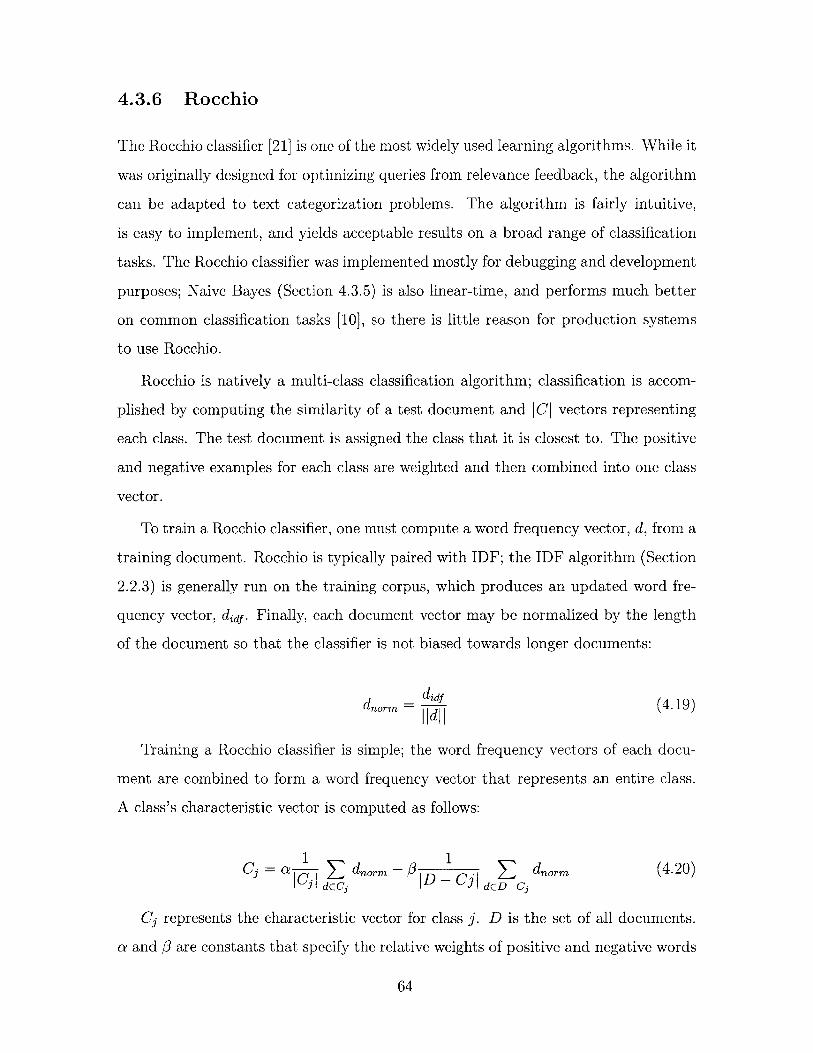
4.3.6 Rocchio
The Rocchio classifier [21] is one of the most widely used learning algorithms. While it
was originally designed for optimizing queries from relevance feedback, the algorithm
can be adapted to text categorization problems. The algorithm is fairly intuitive,
is easy to implement, and yields acceptable results on a broad range of classification
tasks. The Rocchio classifier was implemented mostly for debugging and development
purposes; Naive Bayes (Section 4.3.5) is also linear-time, and performs much better
on common classification tasks [10], so there is little reason for production systems
to use Rocchio.
Rocchio is natively a multi-class classification algorithm; classification is accom-
plished by computing the similarity of a test document and ICI vectors representing
each class. The test document is assigned the class that it is closest to. The positive
and negative examples for each class are weighted and then combined into one class
vector.
To train a Rocchio classifier, one must compute a word frequency vector, d, from a
training document. Rocchio is typically paired with IDF; the IDF algorithm (Section
2.2.3) is generally run on the training corpus, which produces an updated word fre-
quency vector, didf. Finally, each document vector may be normalized by the length
of the document so that the classifier is not biased towards longer documents:
dnorm =didf (4.19)
Training a Rocchio classifier is simple; the word frequency vectors of each docu-
ment are combined to form a word frequency vector that represents an entire class.
A class's characteristic vector is computed as follows:
1 1Ci = OZ 1 dnorm - 0 1 1 dnorn (4.20)
3C |D- CA| dCD-Cd
C, represents the characteristic vector for class j. D is the set of all documents.
a and 0 are constants that specify the relative weights of positive and negative words
64

(i.e. how many negative words it takes to cancel out a positive word). As recom-
mended by [10] we use a = 16 and 7 = 4. To classify a new document, d', one
compares d' to all classifiers Cj using a similarity measure. The document is assigned
the class that it is most similar to. The similarity measure used is the cosine of the
angle between two vectors, which is easily computed as follows:
cos(d', Cj) = dl. * (4.21)|ld'||* ||Cj||
To classify a document d', we compute
ICIargmax 1 cos(d', C3 ) (4.22)
j=1
4.4 Classifier Performance
This section describes performance evaluations of the classifiers in the Haystack Learn-
ing Framework. The goal of this thesis is to develop a robust learning framework,
not to develop a new classifier and perform extensive benchmarking and analysis on
this classifier. As such, the performance metrics used to evaluate the classifiers are
relatively unsophisticated; we simply want to ensure that the classifiers are working
as advertised, and are not buggy.
Section 2.5 describes the methodology used to evaluate classifier performance.
This section contains the results of testing Haystack's classifiers using the previously
defined methodology.
RLSC Parameter Tuning
Rifkin's thesis [19] states that the RLSC algorithm is relatively unaffected by parame-
ter tuning, but I found that this to be far from the case. RLSC has a single parameter,
fA, that quantifies one's willingness to trade off error on the training set with the risk
of overtraining. When run with the fA parameter equal to 1, as recommended in
Rifkin's thesis, binary classification performance was dismal. Empirical testing with
65

different values of fA showed that the best performance was achieved with a much
larger value of fA = 2000.
4.4.1 Binary Classifiers
Binary classifiers are tested using my Personal Spam Corpus and the "acq" and
"wheat" categories of the Reuters corpus.
Spam Corpus
The Spam Corpus contains 3,360 total messages, 1,613 of which are spam and 1,747
of which are not spam. There were 1,694 messages in the test set.
RLSC
Naive Bayes
66
Actual TRUE Actual FALSE
Classified Positive 772 33
Classified Negative 49 840
Statistic Value
Correct predictions 95.1%
Incorrect predictions 4.8%
Sensitivity 0.940
Specificity 0.962
Actual TRUE Actual FALSE
Classified Positive 721 21
Classified Negative 100 852

Reuters "acq"
The Reuters corpus was split into training and test sets, with 5,082 news articles in
the test set, 1,103 of which are in the "acq" category.
Joachims [10] achieves accuracy rates of around 90% using Naive Bayes on the
Reuters "acq" category.
RLSC
Naive Bayes
67
Statistic Value
Correct predictions 92.8%
Incorrect predictions 7.1%
Sensitivity 0.878
Specificity 0.975
Actual TRUE Actual FALSE
Classified Positive 883 94
Classified Negative 220 3885
Statistic Value
Correct predictions 93.8%
Incorrect predictions 6.2%
Sensitivity 0.800
Specificity 0.976
Actual TRUE Actual FALSE
Classified Positive 931 185
Classified Negative 172 3794

Reuters "wheat"
The Reuters corpus was split into training and test sets, with 5,082 news articles in
the test set, 125 of which are in the "acq" category.
Joachims [10] achieves accuracy rates of around 95% using Naive Bayes on the
Reuters "acq" category.
RLSC
Naive Bayes
68
Statistic Value
Correct predictions 92.9%
Incorrect predictions 7.1%
Sensitivity 0.844
Specificity 0.953
Actual TRUE Actual FALSE
Classified Positive 84 10
Classified Negative 41 4947
Statistic Value
Correct predictions 98.9%
Incorrect predictions 1.1%
Sensitivity 0.672
Specificity 0.997
Actual TRUE Actual FALSE
Classified Positive 102 124
Classified Negative 23 4833
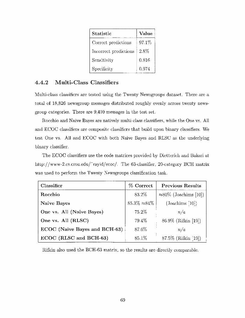
4.4.2 Multi-Class Classifiers
Multi-class classifiers are tested using the Twenty Newsgroups dataset. There are a
total of 18,826 newsgroup messages distributed roughly evenly across twenty news-
group categories. There are 9,410 messages in the test set.
Rocchio and Naive Bayes are natively multi-class classifiers, while the One vs. All
and ECOC classifiers are composite classifiers that build upon binary classifiers. We
test One vs. All and ECOC with both Naive Bayes and RLSC as the underlying
binary classifier.
The ECOC classifiers use the code matrices provided by Dietterich and Bakari at
http://www-2.cs.cmu.edu/~rayid/ecoc/. The 63-classifier, 20-category BCH matrix
was used to perform the Twenty Newsgroups classification task.
Classifier % Correct Previous Results
Rocchio 83.2% f80% (Joachims [10])
Naive Bayes 85.3% ~84% (Joachims [10])
One vs. All (Naive Bayes) 75.2% n/a
One vs. All (RLSC) 79.4% 86.9% (Rifkin [19])
ECOC (Naive Bayes and BCH-63) 87.6% n/a
ECOC (RLSC and BCH-63) 85.1% 87.5% (Rifkin [19])
Rifkin also used the BCH-63 matrix, so the results are directly comparable.
69
Statistic Value
Correct predictions 97.1%
Incorrect predictions 2.8%
Sensitivity 0.816
Specificity 0.974

70

Chapter 5
Cesium
This chapter describes the design and implementation of Cesium, an auto-classification
agent for Haystack, and Haystack's first real autonomous agent.
Cesium's job is to learn a model from a Haystack categorization scheme, and to
apply this model to any new documents in a collection. Cesium produces a set of pre-
dicted class labels for a document, and annotates the document with its predictions.
These annotations are distinct from the document's manually assigned categories, and
while the classifier's predictions are displayed in the UI, the predicted categories do
not affect any other aspect of UI operation; the rest of the Haystack UI is still keyed-
off of the manually assigned category. The classifier's predictions are an unobtrusive
but valuable addition to the categorization UI.
Cesium is backed by the learning framework's Fuzzy Simple Multi-label classifier,
which is described in Section 4.3.1. The aforementioned "fuzziness" allows Cesium
to assert facts about documents with varying degrees of confidence. The fuzziness
extends beyond training, and encompasses the classifier's predictions as well; the
classifier does not make a simple binary decision regarding class membership - a
document is not simply in or out of a class - but, instead, the classifier produces a
list of potential categories, ranked by their likelihood according to the classification
model.
71

5.1 Problem Specification
An auto-classification agent should have the following characteristics:
" The classifier must be able to place documents in more than one category. Some
types of classifiers assume that documents are only a member of exactly one
class. While these classifiers might be appropriate for a traditional e-mail han-
dling program, where an e-mail is located in exactly one folder, Haystack's
flexible categorization scheme requires the flexibility of a multi-label classifier,
which can label a document with any number of categories.
" The classifier must be kept fresh. Training a classifier is a time-consuming
process, and cannot be done incrementally. The auto-classification agent must
conserve system resources (i.e. re-training every time a document is added is
most likely not an option) but maintain a relatively fresh corpus.
" The user must be able to specify arbitrary "training" and "test" sets. While the
notion of a training and set set has little meaning on a real-world classification
system - it is mostly an artificial distinction made in research classifiers - the
user must be able to tell the classifier to learn from a set of documents and to
apply its model and classify another set of documents.
" The classifier must not train over its own predictions, even if its "training" and
"test" sets refer to overlapping collections of documents. The job of a classifier
is to predict new categories for a document, but these predictions may not be
accurate, and the user may not correct all mis-classifications. If the classifier
trains using its predicted data, classification performance will suffer; there must
be a mechanism for distinguishing the predicted categories from the actual,
manually-specified categories.
* The user must be able to correct mis-classifications. The classifier should learn
from its mis-classifications, and it must remember all corrections.
72

5.2 A Cesium Agent's Properties
A Cesium agent has a number of properties that govern how it works:
" The set of training documents. Haystack lets the user define arbitrary cate-
gorization schemes, and an arbitrary number of these categorization schemes
define the training data for Cesium's classifier. A categorization scheme, an
example of which is shown in Figure 5-2, is defined by a set of possible cate-
gories, and the documents in the Haystack that have these categories. As such,
documents that have no category are not considered part of a categorization
scheme, and are not considered by the classifier.
New categorization schemes can be added by dragging and dropping them on
the appropriate place in the Cesium properties page (see Figure 5-1).
* The set of test documents. An Cesium agent can have any number of test
sets, or "autoclassify collections." The Cesium agent monitors these autoclas-
sify collections, and when new documents appear, it annotates them with its
predictions.
An agent's autoclassify collections are the collections where the classifier will
apply its model. Cesium monitors the autoclassify collections for changes, and
when a new document is added, it runs the classifier and annotates that doc-
ument with its predictions. A collection can be added to an agent's list of
autoclassify collections by dragging and dropping the collection in the appro-
priate place in the Cesium properties page (see Figure 5-1).
" Training Schedule. Training is a resource-intensive process, and cannot be done
incrementally. The Cesium agent retrains itself every hour, by default, though
this time period can be adjusted. There are other training schemes, some of
which are documented in Section 2.4.2, but Cesium simply re-trains itself on an
interval.
73

OscarShow all information V Select information sources v
B General Service Properties
This service works on behalf of Mark Rosen.
" Sharing
L Access ControlNo items in list
E Autodassify Colections
J Inbox
9.5.chedule.Last Run Mon Feb 3 04:48 18 EST 2003 Add
Frequency 3600000 Add I
Service Oscar Add j
E categorization Schemes
j My Categorization Scheme
EStandard Properties
2All Properties
8 Locate additional information
No information is available at this time.
Figure 5-1: Cesium Properties. The "Sharing," "Access Control," and "Locate addi-tional information" property headings are provided by Haystack, and are not relevantto this thesis.
74

5.3 Classification and Correction
Z Classification occurs automatically when new documents appear in a Cesium agent's
"autoclassify collections." The predictions of the classifier are distinct from the man-
ually generated labels. This is done for two reasons:
" Classifier inaccuracy. The classifiers discussed in this thesis perform well, but an
80-90% classification accuracy is far from perfect. The UI is currently keyed off
of a document's manually specified labels - all navigation and organization UI
components use the manually specified labels. The classifier's recommendations
are displayed as just that - tentative recommendations - and accomplishing
this requires that the manually generated labels be distinct from the classifier's
predictions.
" The classifier must not train off of its own predictions. The classifier only
trains off of manually labeled categories; classifier performance would suffer if
the classifier trained off of its predicted labels.
5.3.1 The Data Model
A document's category or predicted category is represented by annotating that object
with one of three possible types of annotations:
* memberOf. This assertion is used when a user manually assigns a document to
a category.
* notMemberOf. This assertion is used when a user manually indicates that a
document is not a member of a category.
" predictedMemberOf. This assertion is used by the classifier to predict a docu-
ment's category.
75

A Belief Engine
This data model is inelegant in that it introduces a new type of memberOf assertion,
predictedMemberOf, that represents a specialized form of membership asserted by
a single agent, Cesium. While this is an acceptable short-term fix, if every type of
agent made its own, specialized assertions about class membership, the data model
would quickly become cluttered.
The elegant way to implement predictedMemberOf is to use a belief system. A
belief system takes the disparate memberOf assertions provided by each agent, de-
termines how much we trust each of the assertion's creators, and filters the results
accordingly. A belief system obviates the need for separate types of memberOf asser-
tions such as predictedMemberOf.
5.3.2 Training a Fuzzy Classifier
Much ado has been made about the "fuzziness" of some of the classification algo-
rithms in Chapter 4. A traditional multi-label classifier makes the assumption that
if a document is in set of categories, then it is not in all other categories. While
this assumption is an inaccurate description of Haystack's categorization ontology,
it does have the benefit of generating a large number of negative training examples.
Haystack does provide a mechanism for users to assert that a document is not a mem-
ber of certain categories, but it's unlikely that users will manually negatively label
many documents. Documents will most likely be assigned negative labels only when
the classifier mis-predicts an item's category and the user corrects this prediction;
we estimate that there will be significantly fewer negative examples than positive
examples.
It's likely that there wouldn't be sufficient data to build a robust model if the
classifier trained only on the user's explicit categorizations. We use the traditional
categorization assumption - that a document that is a member of a set of classes is
not a member of all other classes - to generate additional negative training examples,
but we tell the classifier that these examples are "weak."
76

Fuzzy classifiers associate each set of document's labels with a confidence value
that quantifies how certain we are about the document's categorization. We are ab-
solutely certain about manually classified documents, and they are presented to the
classifier with a confidence value of 1.0. Documents generated by the traditional cat-
egorization assumption are presented to the classifier with a much smaller confidence
value.
To summarize:
" Assertions made by the user are presented as concrete examples. If the user
manually labels a document as either a positive or negative example of a cat-
egory, then the document and its label are presented to the classifier with a
confidence value of 1.0.
* Negative examples generated by the traditional categorization assumption are
given weak confidence values. Machine-learning problems typically assume that
if a document is a positive example for a set of classes, then it must be a
negative example for all other classes. This assumption is generally not true
in Haystack, but without this assumption there wouldn't be sufficient numbers
of negative examples in each class for most learning algorithms to generate an
effective model. Class labels generated by this assumption are presented to the
classifier with a weak confidence value.
5.3.3 The Classification User Interface
A good user interface for classification must have the following capabilities:
" The UI must be able to denote that a document is in a category, is not in a
category, or that a document's category is unknown.
" The classifier's predictions must be displayed in a unobtrusive way. The clas-
sifier will be incorrect frequently enough that the classifier's recommendations
should not significantly alter the UI - i.e. the classifier's predictions should not
be used for navigation.
77

Figure 5-2: Haystack's Organize Pane
" Users must be able to correct and validate predictions. If the classifier's predic-
tion is correct, then the user must be able to validate this prediction. Similarly,
if the classifier's prediction is incorrect, then the user must be able to correct
this mis-classification.
" Different predictions have different strengths. Not all predictions are created
equal; the classifier might be very confident about one prediction, but uncertain
about another. The user interface should differentiate between the different
prediction strengths.
Cesium's categorization user interface is simple and easy to use, but contains a lot
of functionality and renders a lot of information. The centerpiece of the categorization
UI is the "Organize" pane, which is displayed in Figure 5-2.
The most important job of a categorization UI is to display membership - i.e.
whether a document is or is not in a category. This is accomplished by a series of
check boxes adjacent to the category names. If a document is in a category - if
there is a memberOf assertion connecting the document with a category - then a
check appears in the check box adjacent to the category. The absence of a check
implies that either the user has not labeled the document, or that the document is
not in that category. The user cannot distinguish between the two cases, but they
78
B Organize
Categorization scheme:My Categorization Scheme ?E] Cardiac muscle (0 items) X0 Family (0 items) -D Favor (0 items) x[_ Friends (0 items) xE Haystack (0 items) XE Health '!) (14 items) -C] Important (0 items) XE Junk (0 items) EE] Lecture (0 items) -E] Politics (0 items) XEl Spam (0 items) -
Create new category:
XCreate]Autoclassify

are represented differently in the underlying data model, and are used differently
by the classifier. Documents that are not in a category have have a notMemberOf
assertion connecting the document and the category, while an unknown category has
either a memberOf or a notMemberOf assertion. To the classifier, documents that are
definitely not members of a category are regarded as concrete negative examples, while
documents with unknown labels are passed on to the classifier as "weak" negative
examples of those categories.
Predictions are displayed in the user interface via a light bulb - if a light bulb
appears next to a category, then the classifier has predicted that the current document
is in the category. The intensity of the color of the light bulb indicates the strength of
the prediction - a deep yellow light bulb indicates that the classifier is fairly confident
in its prediction, while a light yellow light bulb indicates that the classifier is relatively
uncertain of its prediction.
The classifier's predictions can be validated by clicking on the light bulb - clicking
the light bulb will change the tentative predictedMemberOf assertion to a concrete
memberOf assertion, will remove the light bulb from the user interface, and will place
a check next to the category. To correct a classification, a user clicks on a light bulb
and then unchecks the category.
5.4 Oscar
Cesium is the name of a general type of auto-categorization agent backed by a Simple
Multi-Label classifier that learns from a categorization scheme and applies its model
to a collection. To set the machine learning machinery in motion, you must create an
instantiation of a Cesium agent, and configure the Cesium agent's properties. Oscar
is currently the only Cesium agent in Haystack. By default, Oscar trains on any
indexable document, and automatically classifies items in the Haystack Inbox.
Oscar trains over all Haystack content, but new instantiations of Cesium should
probably specialize on a specific type of information. For example, a new classification
agent, Einstein, could be created to categorize research papers.
79

80

Chapter 6
PorkChop: An Outlook Plugin for
Spam Filtering
This section describes the implementation of a spam-filtering Microsoft Outlook plu-
gin using the learning algorithms described in Chapter 4. Outlook was chosen because
it has a dominant market share, and because its API is much more flexible than the
plug-in APIs of other competing programs like Eudora.
Spam Filtering Tools
There are a large number of spam filtering programs out there. A search of down-
load.com for "spam filter" yields over 100 Windows programs - and this excludes
the UNIX universe. This section discusses, in-depth, several popular spain-filtering
programs and techniques.
Spam filtering programs, in general, are far from state of the art. The most
common spam filters these days use rules-based filtering; only recently have naive
bayesian filters started appearing in popular spam detection packages.
Blacklists
Blacklists were the earliest means of spam filtering. A blacklist is a simple concept -
various groups like MAPS, SPEWS, and Spamhaus [26, 27, 25] respond to complaints
81

from users and compile a list of originating domains that are used to send spam. ISPs
that subscribe to the blacklist then block all e-mail messages (or even all network
traffic) from these domains. Early blacklists were met with open arms - blacklists
were viewed by ISPs as a way to reduce the network traffic associated with spam and
therefore lower their costs, all while pleasing their customers [5].However, spammers have adapted well to the challenge posed by blacklists. They
often hop from SMTP server to SMTP server, operating one step ahead of the black-
lists. An article in Network World [4] references a study that found that the MAPS
RBL, one of the most popular blacklists, blocked only 24% of actual spam messages,
but blocked 34% of legitimate messages. Such results are absolutely abysmal and
even the most unsophisticated content-based filters can easily accomplish better clas-
sification performance.
Additionally, the spam blacklist maintainers have made many enemies by adopting
a "shoot first and ask questions later" blacklisting policy. In one rather exceptional
case [4], one customer of the iBill electronic billing service complained to MAPS about
unsolicited e-mail from one of iBill's clients. The e-mail was not even sent from iBill
itself - it was sent by one of iBill's thousands of customers. MAPS not only placed
the accused spammer on their Realtime Blacklist (RBL), but they placed all of iBill's
IP addresses on the blacklist as well. iBill received no warning - only complaints
from customers confused by the blackout - and lost over $400,000 during the four-
day blackout. The blacklist maintainers' heavy-handed tactics have won them few
fans among IS managers at blacklisted companies - "There's no appeals process once
you're blacklisted. The MAPS folks were arrogant and pompous to deal with. They're
out of control."
CRM114
The CRM114 "Controllable Regex Mutilator" is a system to process large data
streams, and has been used to build a Naive Bayes e-mail filtering system. The
author makes impressive claims about the accuracy of the software - it is over 99%
accurate on a corpus of 5,800 messages - but his results have not been independently
82

and rigorously verified.
While most machine learning systems generally try to reduce the number of fea-
tures, both to reduce computational requirements and to decrease the potential for
over training, the CRM114 system tries to generate as many features as possible by
moving a 5-word sliding window over the incoming text and generating subphrases
from this 5 word window. See Section 2.1.1 for more information on CRM114's phrase
expansion algorithm.
Spam Assassin
Spam Assassin is a framework for combining disparate spain detection techniques.
Rather than use one technique - Naive Bayes statistics or rules-based detection algo-
rithms - Spam Assassin provides a framework to combine any number of heuristics.
SpamAssassin maintains a table of different spam detection techniques. Each entry
in the table has two components: 1) code to calculate the specific metric, and 2) the
weight of the metric. Most of the metrics are typical rules-based metrics, but one
of the metrics is the Naive Bayes classification of the e-mail message. To classify a
message, Spam Assassin runs each metric in the table, and adds up the weights of the
triggered metrics; if they exceed a specified threshold, then the message is marked as
spam. Spam Assassin runs a genetic algorithm on the spam detection table, altering
the weights of each classification technique until it maximizes the classifier's efficiency.
There are a number of possible ways to combine traditional rules-based systems
and Naive Bayes classifiers, and the Spam Assasin designers believe that they have
found the best way to combine the power of the two respective approaches. It's easy
to write a rule to detect a malformed e-mail message header (indicative of spam),
but it's much more difficult to, for example, determine a numerical measure of how
malformed a header is, and then use that measure as a feature in a message's word
frequency vector.
The Spam Assasin team experimented with using Naive Bayes to learn different
measures of "spammishness" in the text (i.e. the number of ALL CAPS words), but
found this to be ineffective. Most spam metrics are positive - i.e. they are designed
83

to identify spam, rather than identify non-spam - but machine learning algorithms
work best when the feature vectors contain both positive and negative metrics. The
rule table used in Spam Assassin is additive, which is better suited for positive spam
metrics; if a rule is triggered, then the weight associated with that rule is added to the
spain metric. Naive Bayes is implemented as a single entry in the rule table, though
the genetic algorithm usually gives a high weight to the output of the Naive Bayes
classifier.
6.1 PorkChop Implementation
The Outlook spam filter plugin uses the learning framework provided in Chapter 4.
The Outlook filter uses the binary classification algorithms provided by the learning
architecture - specifically the Regularized Least Squares Classification algorithm - to
classify spam.
When PorkChop is first installed, it must be initialized with e-mail messages from
the user's Inbox; PorkChop does not come pre-programmed with a spam database.
When new messages are downloaded from the e-mail server, PorkChop runs these
messages through the learning framework and produces a predicted classification for
each message. Messages that are suspected to be spam are invisibly marked as such
via an Outlook CustomProperty, and are moved by Outlook's filtering mechanisms to
a special Spam folder. New buttons in the Outlook interface are provided to handle
mis-classified e-mail.
Training the classifier is a resource-intensive process, and cannot be done incre-
mentally. The classifier can be trained on demand, but it is automatically run when
there are more than 100 new messages in the "to be trained" queue, or when there is
a message in the queue that has been around for more than eight hours.
In addition to the binary classifier, PorkChop uses whitelists to properly classify
e-mail. The whitelists are manually maintained - users must add e-mail addresses.
Messages from users on the whitelist are not run through the classifier; whitelists
reduce both false positives and total total computation time.
84

The Haystack Learning Framework is written in Java, but it takes a substantial
amount of work to bridge the gap between Microsoft Outlook and Java. Microsoft
Outlook provides a very robust scripting interface via Visual Basic for Applications
(VBA). While VBA is well-suited for GUIs and other lightweight tasks, more heavy-
duty tasks are often offloaded onto COM modules. COM stands for Component
Object Model, and is Microsoft's distributed object system. Java modules can export
COM interfaces, but, unfortunately, Java support for COM ties you to a specific VM;
Microsoft provides support for COM interfaces in its VM, while Sun's VM supports
COM interfaces via JavaBeans. SWT provides VM-independent COM interface sup-
port, but then you're tied to the SWT library; the SWT library comprises about a
megabyte - not exactly lightweight.
Ironically, the easiest way to interface the Java machine learning code with Out-
look's VBA is to use C++. Microsoft Visual C++ has excellent support for COM
development, and JNI allows C++ functions to call Java code. Because there were
only a few functions (addDocument, train, and classify), it was easy to write a C++
COM wrapper for the Java learning functions. When an action needs to be performed
in Outlook (i.e. a message must be classified), Outlook VBA code calls C++ COM
code, which uses JNI to invoke the Haystack Learning Framework.
6.2 Performance
PorkChop uses whitelists and the RLSC algorithm to filter spam messages from Out-
look. The performance metrics in Section 4.4 show that RLSC can distinguish spam
with roughly 95% accuracy. This is impressive, but there are better frameworks for
spam detection.
SpamAssassin, described in Section 6, uses a combination of static rules and dy-
namic machine learning algorithms (Naive Bayes) to detect spam. While machine
learning algorithms perform extraordinarily well by themselves, some attributes of
spam are extremely difficult to quantify and present as a feature to a machine learn-
ing algorithm. For example, spam e-mails often have malformed e-mail headers; it's
85

vuuu I Wuay - trersonai romersCalendarContactsDeleted Items (1250)DraftsEuro-share
B (2)-( tiubTopS (19)
Unkown Senders (45)- Journal
- Junk E-mail (4)I Mach5 ArchiveNotes
- Outbox- lItems
S5pam)
A~i
AAAAAAAA
Mike Lan... RE: RE: MidiNotate Order R020712-10464Mike Lan... Fwd: RE: MidiNotate Order R020712-10464Mike Lowell Re: heyMike Lowell heyMike Lan... Application previewsMike Lan... Analyzer 3 testingMike Lan... Re: PatentingMike Lan... Re: RegistrationMike Lan... SupportMke Lan... Re: RT* 9184Mike Lan... Message for ConnyMike Lan... Code generator for fs3
L~I
Figure 6-1: PorkChop in action
difficult to make a machine learning algorithm learn whether a header is well-formed
or malformed, but it's easy to write a rule that determines the validity of an e-mail
header.
SpamAssassin's hybrid approach to spam detection is more robust than Pork-
Chop's machine-learning only spam detection algorithms. Were I to write PorkChop
again, I would not code it as a stand-alone application; I would incorporate it into
the SpamAssassin codebase.
86
Mon 7/15/2002...Wed 7/312002 ...
Wed 7/312002 ...Fri 612112002 6...Fri 6/21/2002 5...Fri 6121/2002 9...Thu 6120/2002 ...Thu 6/20/2002 ...Thu 6/20/2002 ...
Thu 6/20/2002 ...
Thu 6/20/2002 ...

Chapter 7
Cholesterol
7.1 Introduction
Resource Description Framework, or RDF, forms the backbone of Haystack; all data
in Haystack is stored in RDF. Haystack's RDF store is called Cholesterol, and because
of RDF's central role in Haystack, the design, features, and performance of Cholesterol
have a major effect on Haystack. RDF statements are triples - a subject, predicate,
and object, and Cholesterol is a database that is purpose-build to store these RDF
triples.
Because Cholesterol is the backbone of Haystack, it is placed under a very high
query load. For Haystack to be sufficiently responsive to user interface commands,
Cholesterol must be able to execute thousands of queries per second over a typically
80-120 megabyte corpus. Cholesterol bears little resemblance to the common notion
of a database - i.e. one that supports transactions, tables, and can be manipulated
using SQL. Clients interface with Cholesterol using a Java API; the overhead of
creating a connection and parsing the SQL query is too great to achieve the kind of
performance expected by Cholesterol. Unlike SQL, which has a rich query syntax,
Cholesterol's query interface is very minimalistic; the only tools one has to work with
are wildcards and joins.
As of the writing of this thesis, there are three versions of Cholesterol. Cholesteroll
is the first incarnation of the Cholesterol database, and was a hasty C++ port of a
87

Java database. Cholesteroll indexed its RDF triples with an eye toward the common
case; as long as the predicate of a query is not a wildcard, Cholesteroll can execute the
query fairly quickly. However, because Cholesteroll was quickly written, its code was
not very readable, and the complexity of the code led to a number of nagging, virtually
unsolvable bugs. Cholesterol2 uses the same architecture as Cholesteroll, but is
completely rewritten with the goal of improving code readability. Unfortunately, due
to memory copying overhead in the query execution code, Cholesterol2 is only half
as fast as Cholesteroll. Cholesterol3 is a completely new take on the Cholesterol
database that manages its own memory and indexes all fields.
7.2 Cholesterol API
This section discusses the Cholesterol API that is implemented by all Cholesterol
databases. The Java interface IRDFStore defines the Java interface that must be
implemented by an RDF Store, but because of the need for speed, all three Cholesterol
databases are written in C++. The CholesterolRDFStore implements IRDFStore,
and specifies that the following JNI native interfaces must be provided by a C++
Cholesterol database.
class CholesterolRDFStorenative void doNativeInit(String basePath);native void doNativeKill();
native boolean add(String subj, String pred, String obj, String id);
native boolean addAuthored(String subj, String pred, String obj, String id, Object [ authors);
native void remove(String ticket, Statement s, Resource[] existentials) throws ServiceException;
native Set query(String ticket, Statement[] query, ResourceE] variables, Resource[] existential)throws ServiceException;
native Set queryMulti(String ticket, Statement[] query, Resource[] variables,
Resource[] existential, RDFNode [][] hints) throws ServiceException;
native boolean contains(String subj, String pred, String obj);
native RDFNode extract(String ticket, Resource subject, Resource predicate, RDFNode object)
throws ServiceException;
native Resource[] getAuthors(String ticket, Resource id) throws ServiceException;native Resource[] getAuthoredStatementIDs(String ticket, Resource author) throws ServiceException;
native Statement getStatement (String ticket, Resource id) throws ServiceException;
}
Figure 7-1: The native interface provided by each C++ Cholesterol database
88

" doNativeInit. The doNativeInit function initializes the Cholesterol database.
* doNativeKill. The doNativeKill function indicates to Cholesterol that Haystack
is shutting down, and that Cholesterol can begin to free up its internal data
structures. However, practically, queries continue to be issued to Cholesterol
even after the doNativeKill function is called. Implementations of doNativeKill
should flush any buffers to ensure that Cholesterol's state is written to disk,
but doNativeKill should not delete any data structures because Cholesterol
must handle queries even after doNativeKill is called.
" add. The add method adds an RDF triple, plus a unique identifier, to the
Cholesterol database. After the add function is called, subsequent calls to query
must reflect the updated database state. However, Cholesterol is not a trans-
actional database; after a crash, Cholesterol does not have to recover the exact
pre-crash state, which allows for faster add performance. Adds are written to
a log (more details in Section 7.4.3).
* addAuthored. The addAuthored method has the same interface as add, ex-
cept that it takes an additional argument that represents the authors of a spe-
cific statement. The authors parameter is an array of Object classes, whose
toString() values are stored in the database and are used to answer queries to
the getAuthors and getAuthoredStatementID methods, which are part of the
belief layer described in M. Zhurakhinskaya's thesis [29].
* remove. The remove function removes the given RDF triple from the database.
The RDF triple may be fully specified (i.e. no wildcards), or it may include
wildcards. The wildcard matching scheme is implemented in the same man-
ner as in the query method. C++ implementors of remove must make a JNI
call to the CholesterolRDFStore.addToRemoveQueue method, which is used to
implement triggering. Removes are written to a log (more details in Section
7.4.3).
" query. The query method queries the Cholesterol database. The query method
89
takes an arbitrary number of RDF triples that may contain wildcards. If a
query has more than one RDF triple, then Cholesterol performs a join across
the triples. Section 7.3 discusses Cholesterol queries in detail. The existential
argument to query contains an array of RDFNodes which represent the existen-
tials used in the query. The variables argument contains an array of Resources
that must be a subset of the Resources in the existential argument.
The query method returns a Set that contains all of the possible existential
bindings. Each element of the Set is an array of RDFNodes, and the existentials
in the RDFNode array are stored in the same order as the existentials were
specified in the variables array. For example, if the first element of variables is
the existential ?x, then the first element of every RDFNode array corresponds
to the value of the existential ?x.
" queryMulti. The queryMulti method has the same interface as query, with the
addition of a hint parameter. This parameter provides data that restricts the
values of some variables in the query. The data in the n-th row of the hint
parameter represents the set of all allowed values for the n-th existential in the
existential parameter. If data is present for an existential (i.e. the row is not
null), then that existential is constrained to one of the given values. The hint
parameter is used to optimize federation, which is an inter-database join.
" contains. The contains method takes as an argument a single RDF triple (no
wildcards allowed), and returns true if that triple exists in the database.
" extract. The extract method is a specialized form of query. Exactly one of the
arguments to extract must be null, which implies a wildcard in that position.
The extract method will then execute the query defined by the RDF triple and
return one of the possible values of that existential. If there are many values
for the existential, then extract is free to return any possible value.
" getAuthors. The getAuthors method returns all authors of a given statement
ID (or null if the statement has no authors). The getAuthors method is used
90

to implement authoring, which is described in M. Zhurakhinskaya's thesis [29].
" getAuthoredStatementlDs. The getAuthoredStatementIDs returns the state-
ment IDs created by a given author. A statement ID uniquely identifies a
statement, and is specified in calls to the add or addAuthored methods. The
getAuthoredStatementIDs method is used to implement authoring, which is
described in M. Zhurakhinskaya's thesis [29].
" getStatement. The getStatement method returns the RDF triple associated
with the given statement ID. The statement ID uniquely identifies a statement,
and is specified in calls to the add or addAuthored methods.
Cholesterol may be called from within multi-threaded client programs, and must,
therefore, be thread-safe.
7.3 Queries
This section describes how to query
is used in all subsequent examples.
a Cholesterol database. The following database
Cholesterol supports a very minimalist query interface. A query is composed of
an arbitrary number of RDF statements, which may or may not contain wildcards.
A wildcard - also called an existential - will match any possible row. For example
mark likes ?x matches:
91
Subject Predicate Object
mark likes melanie
mark likes robert
melanie likes joe
beth likes joe
mark hates kim
melanie likes steve
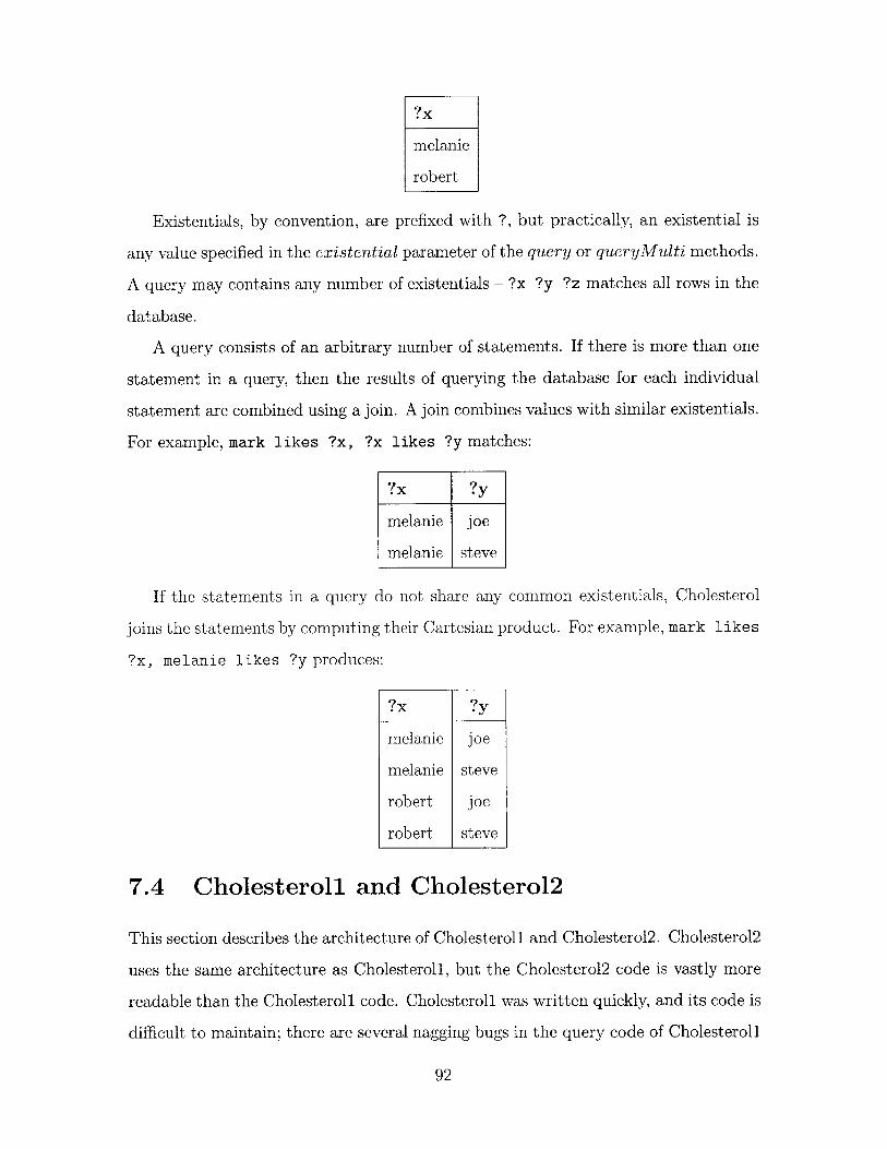
?X
melanie
robert
Existentials, by convention, are prefixed with ?, but practically, an existential is
any value specified in the existential parameter of the query or queryMulti methods.
A query may contains any number of existentials - ?x ?y ?z matches all rows in the
database.
A query consists of an arbitrary number of statements. If there is more than one
statement in a query, then the results of querying the database for each individual
statement are combined using a join. A join combines values with similar existentials.
For example, mark likes ?x, ?x likes ?y matches:
?x ?y
melanie joe
melanie steve
If the statements in a query do not share any common existentials, Cholesterol
joins the statements by computing their Cartesian product. For example, mark likes
?x, melanie likes ?y produces:
?x ?y
melanie joe
melanie steve
robert joe
robert steve
7.4 Cholesteroll and Cholesterol2
This section describes the architecture of Cholesteroll and Cholesterol2. Cholesterol2
uses the same architecture as Cholesteroll, but the Cholesterol2 code is vastly more
readable than the Cholesteroll code. Cholesteroll was written quickly, and its code is
difficult to maintain; there are several nagging bugs in the query code of Cholesteroll
92

have proven to be nearly impossible to fix. Cholesterol2 is a ground-up rewrite of
Cholesteroll that fixes the query bugs and has a much more elegant design. Unfortu-
nately, due to not-clearly-understood causes - most likely memory copying overhead
in the query code - Cholesterol2 is about twice as slow as Cholesteroll.
Because Cholesteroll and and Cholesterol2 have the same architecture, they are
discussed together.
7.4.1 Indexing
Conceptually, the RDF store can be viewed as a flat table of RDF triples. Queries
are composed of any number of statements, with an arbitrary number of wildcards
in each statements. While each RDF triple may have an arbitrary wildcard pattern,
some types of queries are performed much more frequently than other types of queries.
Specifically, most queries do not have an existential predicate, and Cholesteroll and
Cholesteroll optimize for this common case.
Predicate Table for "likes"
Subject -> Object Object -> Subject
mark melanie, robert melanie melanie, robert
melanie joe, steve robert joe, steve
beth joe joe joe
kim melanie, robert
steve joe, steve
Figure 7-2: A predicate table for the predicate "likes"
The triples in a database are organized into "tables," where each unique predicate
has its own table. The mapping between predicates and their tables is stored in a
hash table; given a literal predicate, it is very efficient to retrieve its table. However,
93

if the predicate in a query is an existential, then Cholesterol must iterate through
every predicate in the database to execute the query.
Within each table, there are two indexes; one that associates subjects with objects,
and one that associates objects with subjects. The indexes are implemented as hash
tables, which allows for efficient lookup of subject and object data. Given a literal
subject, it's very efficient to retrieve the object parameter of all triples in the database
with that subject. Similarly, given a literal object, the other index can be used to
efficiently retrieve the subject parameter of all triples in the database with that literal
object.
This indexing structure means that the following queries can be executed quickly:
?x predicate object, subject predicate ?x, and ?x predicate ?y.
7.4.2 Joins
In Cholesterol's simple query interface, joins and wildcards are the only way to extract
data from the database. Joins are used commonly and must be very efficient. A
join occurs when a Cholesterol query consists of more than one RDF statement;
Cholesterol executes each RDF statement separately, and combines the results of
each single-statement query using a join.
Queries are implemented internally via executing one statement at a time; the
database knows how to query itself using a single statement with any pattern of
wildcards. A higher-level join engine combines the results of separate single-statement
queries. Figure 7-3 is a listing of the Cholesterol2 join code and shows the modularity
of the query execution engine.
The statements that compose each query could be executed individually, and after
every statement has been processed, combined by the join engine. However, this is
inefficient; once you have executed one statement that contains one existential, you
have constrained the value of that existential. Subsequent queries and joins can only
reduce the total set of possible values for that existential.
Once Cholesterol has executed a query involving at least one existential, it stores
a list of all possible values for that existential. Ensuing queries that involve that exis-
94

CResultSet *CCholesterolDatabase: :doQuery(const CStatementArray &statementArray)
if (statementArray.NumStatements() == 0)return NULL;
else if (statementArray.NumStatements() == 1)return doSingleStatementQuery(statementArray.GetStatement(0));
else{
CResultSet *pAllResults = new CResultSet(statementArray.GetNumExistentials());CResultSet *r = doSingleStatementQuery(statementArray.GetStatement(0));if (r == NULL) return NULL;pAllResults->Append(r);delete r;
for (nt q=l;q<statementArray.NumStatements();q++)
CQueryRestriction qr(pAllResults);CResultSet *nr = doSingleStatementQuery(statementArray.GetStatement(q), &qr);if (nr == NULL) return NULL;pAllResults->Join(nr);delete nr;
}
return pAllResults;}
}
Figure 7-3: The Cholesterol2 Join Code
tential, rather than examining all possible values for the existential, can examine only
the known values for the existential. One can illustrate the usefulness of constraining
an existential using the example database defined in Table 7.3 and the example query
mark likes ?x, ?x likes ?y.
After the first statement has been executed, the ?x variable is constrained to
either melanie or robert. If ?x likes ?y were to be executed independently, it
would return 5 rows (nearly all of the rows in the database). However, because
of the constraints on ?x, ?x likes ?y can be executed as melanie likes ?y and
robert likes ?y. The more constrained the existentials in a statement are, the
faster subsequent single-statement queries will execute.
7.4.3 Logging
Cholesteroll and Cholesterol2 serialize the contents of their database using a log. The
log is relatively simple; it is a sequential record of every add or remove that has been
performed on the database. To load the database, all adds and removes in the log are
simply re-played. There is currently no optimization to remove redundant log lines;
95

rows that are added and then removed still exist in the log.
Cholesteroll and Cholesterol2 originally enforced a strict coherency model; after
an add or remove successfully executed, the database was required to recover to
the exact same pre-crash state and had to reflect every successfully executed add or
remove operation. However, this restriction requires writing to disk after every add
or remove, which severely impacts Cholesterol's performance.
This strict coherency requirement has been relaxed, and writes to the log are now
cached in memory, and are flushed to disk only when the cache becomes full. This
means that if Cholesterol crashes abruptly, the most recent database modifications
may be lost. However, this is an acceptable price to pay for the nearly 2x performance
improvement that accompanies cached log writes.
7.4.4 Locking
Cholesterol is called simultaneously from different threads in Haystack; to prevent
race conditions and data corruption, it must place locks around its data structures.
Some testing was performed, and locks in both Windows and Linux are very
inexpensive; there is virtually no overhead to obtain a lock. As such, Cholesterol uses
very fine-grained locks. There is a lock for nearly every individual data structure, and
locks are held as briefly as possible - only over accesses to a single data structure.
If locks were expensive to obtain, more coarsely-grained locking would be used; i.e.
there would be a single lock across the entire add function.
Cholesterol does not use typical critical sections or mutexes; it uses custom read-
write locks. These read-write locks allow multiple threads to read from the same data
structure, but if a thread wishes to write to a data structure, it must have exclusive
access.
7.4.5 Resource IDs
Cholesterol implements a basic form of compression to reduce total memory consump-
tion and to make some internal computation more efficient. Strings are represented
96

internally as integer resource IDs. At all entry points - i.e. the add or query method
- strings are translated into integer resource IDs. The reverse occurs at all exit
points; for example, when the query method returns, all of the internal resource IDs
are translated to strings. Not only does this reduce memory consumption - a string
exists only once in memory, even if it exists multiple times in the database - it also
speeds up internal computation. It is much more efficient to compare two integral
resource IDs than it is to compare two null-terminated strings.
The downside of using resource IDs is that there is a central bottleneck that all
methods must access before they execute, but profiling has found that resource ID
translation takes up a negligible amount of time. The majority of the time is spent
inside of the query and add functions, where all computation is done using the integer
resource IDs.
7.5 Cholesterol3
Cholesterol3 uses a dramatically different architecture than Cholesteroll or Choles-
terol2. Older versions of Cholesterol were fairly fast, but they had a large memory
footprint, and, unfortunately, the primary assumption of the index structure - that
most query predicates are not existential - is not true a significant portion of the
time.
Cholesteroll and Cholesterol2 load the entire database into memory. Theoreti-
cally, the operating system should efficiently send unused portions of memory out to
disk and load them back in if they are needed, but, empirical testing has shown that
Cholesterol generates an abnormally large number of page faults, even on systems
that should have enough physical memory to store the entire database. Cholesterol3
implements its own custom memory management system.
While all versions of Cholesterol support queries with arbitrary patterns of wild-
cards, Cholesteroll and Cholesterol2 optimize for what is a common case - the predi-
cates of each query are literal. While this is true the majority of the time, queries with
existential predicates execute very slowly. Cholesterol3 has a more robust indexing
97

system.
7.5.1 Memory Management
An average Haystack store contains about 500,000 RDF triples that comprise 80 to
120 megabytes of data. This should, theoretically, not be a problem for a modern
operating system's virtual memory facilities. The operating system is supposed to
send unused portions of memory out to disk - to a page file - and load them back into
memory on demand. Unfortunately, empirical testing has shown that the operating
system makes poor decisions about which portions of memory to unload; even on
systems with much more physical memory than the 80-120 megabyte Cholesterol
footprint, Cholesterol has an abnormally large number of page faults. The OS's own
memory management algorithms are, unfortunately, inadequate for applications such
as Cholesterol, which deal with large data sets and are highly dependent on memory
access speeds.
Cholesterol implements its own memory manager. The basic block of the Choles-
terol memory manager is the node, which contains a value and a number of indexes
that contain triples with that value. For example, a predicate node contains the
predicate itself, and then hash tables that index the subjects and object parameters
of triples with that specific predicate. A predicate node looks much like the table
described in Figure 7-2.
Cholesterol starts a watcher thread which monitors the total number of nodes
loaded into memory. If there are too many nodes in memory, the watcher thread
locks the database and then writes nodes to disk. Cholesterol decides which nodes to
write to disk using the least recently used (LRU) algorithm - each node remembers its
last access time, and the oldest nodes are written to disk. If the nodes are requested
- i.e. they are needed for a query - then they are loaded back in from disk.
The paging implementation is far from complete. If a node is paged to disk and
then loaded back in, the next time it is paged to disk, it will be written to in a
new location. Thus, given a database which contains more nodes than the maximum
number of nodes allowable in memory at a single time, the total disk space consumed
98

by Cholesterol will grow as queries are performed. When a query is executed, it may
touch old pages, which must be loaded into memory. As new queries are executed,
these pages will become old again and will be paged out to disk again, but in a new
location. Even if no new nodes are added, the disk footprint of the database will
increase.
Cholesterol3 makes extensive use of memory mapped files; rather than allocating
internal memory using malloc, most data is stored in a memory mapped file.
7.5.2 Indexing
All versions of Cholesterol support arbitrary queries, but Cholesteroll and Choles-
terol2 optimize for common-case queries. Specifically, queries with existential predi-
cates may take a long time to execute, as Cholesteroll and Cholesterol2 must traverse
every unique predicate in the database.
Cholesterol3 improves upon the older indexing schemes by indexing on every field,
rather than just on predicate. In Cholesteroll and Cholesterol2, there is a table
for every unique predicate, and a hash table makes it efficient to retrieve the table
associated with each predicate. Within each table, there are separate hash tables
that index the subject and object parameters of triples with the specified predicate.
This table structure is discussed in Section 7.4.1 and Figure 7-2.
Cholesterol3 uses the same table abstraction, but stores a table for the subject,
predicate, and object. A subject table, for example, is keyed on the subject of a RDF
triple, and contains indexes of the predicate and object. This means that all queries
with identical numbers of existentials are executed in the same manner, regardless of
the position of the existentials.
This index structure duplicates the database many times over, and thus consumes
a large amount of memory. Cholesterol3 allows you to revert back to the old-style
indexes; the new index structure consumes too much memory for most machines.
99

100

Bibliography
[1] S. De Brabanter, J. Lukas, and L. Vandewalle. Weighted least squares support
vector machines: robustness and sparse approximation.
[2] T. G. Dietterich and G. Bakiri. Error-correcting output codes: a general method
for improving multiclass inductive learning programs. In T. L. Dean and K. McK-
eown, editors, Proceedings of the Ninth AAAI National Conference on Artificial
Intelligence, pages 572-577, Menlo Park, CA, 1991. AAAI Press.
[3] Glenn Fung and 0. L. Mangasarian. Proximal support vector machine classifiers.
In Knowledge Discovery and Data Mining, pages 77-86, 2001.
[4] S. Gaudin and S. Gaspar. The spam police: Tactics used by self-appointed spam
fighters come under fire, September 2001.
[5] Paul Graham. Filters vs. blacklists.
[6] Paul Graham. A plan for spam.
[7] Paul Graham. A plan for spam, August 2002.
[8] David Huynh, David Karger, and Dennis Quan. Haystack: A platform for cre-
ating, organizing and visualizing information using RDF.
[9] Fax Internet Technical Resources: Electronic Mail (Email) and Postal Mail.
http://www.cs.columbia.edu/ hgs/internet/email. html.
[10] Thorsten Joachims. A probabilistic analysis of the Rocchio algorithm with
TFIDF for text categorization. In Douglas H. Fisher, editor, Proceedings of
101

ICML-97, 14th International Conference on Machine Learning, pages 143-151,
Nashville, US, 1997. Morgan Kaufmann Publishers, San Francisco, US.
[11] Thorsten Joachims. Text categorization with support vector machines: learning
with many relevant features. In Claire N6dellec and Celine Rouveirol, editors,
Proceedings of ECML-98, 10th European Conference on Machine Learning, pages
137-142, Chemnitz, DE, 1998. Springer Verlag, Heidelberg, DE.
[12] Thorsten Joachims. A statistical learning model of text classification with sup-
port vector machines. In W. Bruce Croft, David J. Harper, Donald H. Kraft, and
Justin Zobel, editors, Proceedings of SIGIR-01, 24th ACM International Con-
ference on Research and Development in Information Retrieval, pages 128-136,
New Orleans, US, 2001. ACM Press, New York, US.
[13] D. Lewis. Representation and Learning in Information Retrieval. PhD thesis,
Unversity of Massachusetts, 1991.
[14] A. McCallum and K. Nigam. A comparison of event models for naive bayes text
classification, 1998.
[15] M. F. Porter. An algorithm for suffix stripping. Program, 14(3):130-137, 1980.
[16] Apache Lucene Project. http://jakarta.apache.org/lucene/.
[17] J. Rennie. Text classification. Talk for 9.250, April 2002.
[18] Jason D. M. Rennie and Ryan Rifkin. Improving multiclass text classifica-
tion with the Support Vector Machine. Technical Report AIM-2001-026, Mas-
sachusetts Insititute of Technology, Artificial Intelligence Laboratory, 2001.
[19] R. Rifkin. Everything Old Is New Again: A Fresh Look at Historical Approaches
in Machine Learning. PhD thesis, MIT, 2002.
[20] Ellen Riloff. Little words can make a big difference for text classification. In Ed-
ward A. Fox, Peter Ingwersen, and Raya Fidel, editors, Proceedings of SIGIR-95,
102

18th ACM International Conference on Research and Development in Informa-
tion Retrieval, pages 130-136, Seattle, US, 1995. ACM Press, New York, US.
[21] J. Rocchio.
1971.
Relevance Feedback in Information Retrieval. Prentice-Hall, Inc.,
[22] Bernhard Schlkopf, Ralf Herbrich, Alex J. Smola, and Robert C. Williamson. A
generalized representer theorem.
[23] J. R. Shewchuk. An introduction to the conjugate gradient method without the
agonizing pain. http://www-2.cs.cmu.edu/ jrs/jrspapers.html, August 1994.
[24] Kai Shih, Yu han Chang, Jason Rennie, and David Karger. Not too hot, not too
cold: The bundled-svm is just right!
[25] SpamHaus. spamhaus.org.
[26] Mail Abuse Prevention System. mail-abuse.org.
[27] Spam Prevention Early Warning System. spews.org.
[28] Y. Yang and X. Liu. A re-examination of text categorization methods. In 22nd
Annual International SIGIR, pages 42-49, Berkley, August 1999.
[29] Marina Zhurakhinskaya. Belief layer for haystack. Master's thesis, MIT, May
2002.
103