E-GOVERNMENT ADOPTION MODEL BASED ON THEORY OF

PLANNED BEHAVIOR: EMPIRICAL INVESTIGATION

A THESIS SUBMITTED TOTHE GRADUATE SCHOOL OF INFORMATICS INSTITUTE

OFTHE MIDDLE EAST TECHNICAL UNIVERSITY

BY

�RFAN EMRAH KANAT

IN PARTIAL FULFILLMENT OF THE REQUIREMENTS FOR THE DEGREE OFMASTER OF SCIENCE

INTHE DEPARTMENT OF INFORMATION SYSTEMS

JULY 2009

Approval of the Graduate School of Informatics Institute.

Prof. Dr. Nazife BaykalDirector

I certify that this thesis satis�es all the requirements as a thesis for the degree ofMaster of Science.

Prof. Dr. Yasemin Yard�mc�Head of Department

This is to certify that we have read this thesis and that in our opinion it is fullyadequate, in scope and quality, as a thesis for the degree of Master of Science.

Asst. Prof. Dr. Sevgi ÖzkanSupervisor

Examining Committee Members

Prof. Dr. Kadir Varo§lu (Ba³kent University, BA)

Asst. Prof. Dr. Sevgi Özkan (METU, IS)

Dr. Ali Arifo§lu (METU, IS)

Asst. Prof. Dr. Tu§ba Temizel (METU, IS)

Asst. Prof. Dr. P�nar �enkul (METU, CENG)

I hereby declare that all information in this document has been ob-

tained and presented in accordance with academic rules and ethical

conduct. I also declare that, as required by these rules and conduct,

I have fully cited and referenced all material and results that are not

original to this work.

Name, Last name : �rfan Emrah Kanat

Signature :

iii

ABSTRACT

E-GOVERNMENT ADOPTION MODEL BASED ON THEORY OF

PLANNED BEHAVIOR: EMPIRICAL INVESTIGATION

Kanat, �rfan Emrah

M.S., Department of Information Systems

Supervisor: Asst. Prof. Dr. Sevgi Özkan

July 2009, 87 pages

The e-government phenomena has become more important with the ever increasing

number of implementations world wide. A model explaining the e-government adoption

and the related measurement instrument �a survey� had been developed and validated in

this study. In a post technology acceptance model (TAM) approach, theory of planned

behavior (TPB) was extended to �t the requirements of e-government context. The

adoption of student loans service of the higher education student loans and accommo-

dation association (KYK) was investigated to obtain data for empirical validation. The

instrument was administered to over four-hundred students and partial least squares

path modeling was employed to analyze the data. The results indicate that the model

was an improvement over TAM in terms of predictive power. The constructs investi-

gated in the study successfully explained the intention to use an e-government service.

Keywords: E-Government, Citizen Adoption, Adoption Models, Structural Equation

Modelling, Partial Least Squares Path Modelling

iv

ÖZ

PLANLI DAVRANI� TEOR�S�NE DAYALI B�R E-DEVLET

BEN�MSENMES� MODEL�: AMP�R�K �NCELEME

Kanat, �rfan Emrah

Yüksek Lisans, Bili³im Sistemleri Bölümü

Tez Yöneticisi: Yard. Doç. Dr. Sevgi Özkan

Temmuz 2009, 87 sayfa

E-devlet fenomeni say�s� dünya çap�nda her geçen gün artan uygulamalar�yla daha da

önemli hale gelmektedir. Bu çal�³mada e-devletin vatanda³lar taraf�ndan benimsen-

mesini aç�klayan bir model ve modelle ba§lant�l� bir ölçüm arac� �bir anket� geli³tirildi

ve do§ruland�. Teknoloji Benimsenmesi Modeli (TBM) sonras� bir yakla³�m içerisinde,

Planl� Davran�³ Teorisi (PDT) e-devlet kapsam�na uyacak ³ekilde geli³tirildi. Yüksek

ö§retim kredi yurtlar kurumu (KYK) ö§renci kredileri servisi modelin deneysel do§ru-

lamas�nda veri sa§lamak için kullan�ld�. Ölçüm arac� dörtyüzün üzerinde ö§renciye

uyguland� ve elde edilen veri parçal� en küçük kareler yol modelleme ile do§ruland�.

Sonuçlar modelin TBM üzerine tahmin gücü aç�s�ndan bir ilerleme oldu§unu ve mod-

elde kullan�lan yap�lar�n bir e-devlet servisini kullanma niyetini ba³ar�yla aç�klad�§�n�

ortaya koydu.

Anahtar Kelimeler: E-Devlet, Vatanda³ Benimsemesi, Benimseme Modelleri, Yap�sal

Denklem Modelleme, Parçal� En Küçük Kareler Yol Modelleme

v

ACKNOWLEDGMENTS

I would like to thank my supervisor Asst.Prof.Dr. Sevgi Özkan and Asst.Prof.Dr. Tu§ba

Ta³kaya Temizel for their guidance and the discipline they provided through out my

thesis.

I would like to present my thanks to the faculty and the sta� of Informatics Institute,

for their contributions to my education since my enrollment. Sibel Gülnar deserves

special mention for her care and support.

It would only be fair to say that without Selda Eren's invaluable friendship and

mentoring that this thesis would have never came through. Her experience into this

painful process greatly eased my pains. I also would like to thank my home-mate, gym-

buddy and brother Emre Sezgin for the support and friendship he provided through

out these years we have been together. The rootbeer team �Mete Özay, Ça§lar �enaras

and Ufuk Dumlu� for all the fun and joy we had together and to my fellow system

administrators, Kerem Ery�lmaz and Adnan Öztürel, for covering for me during the

writing of this thesis.

I would like to thank the open source society as a whole for providing us with such

wonderful tools for free. This study was carried out solely with various open source

tools. While all were very helpful, the following deserve a special place because of their

most considerable contributions. Canonical inc. and the ubuntu society for bringing

Ubuntu to life, the wonderful free operating system. The R development core team for

the most �exible statistical tool available to mankind. LATEX development team for the

greatest typesetting system ever came to existence.

I have to express my deepest gratitude to my parents for the genetic material and

other material bene�ts they provided and to my sister for brightening my life.

vi

To one particular tabby cat...

vii

TABLE OF CONTENTS

ABSTRACT . . . . . . . . . . . . . . . . . . . . . . . . . . . . . . . . . . iv

ÖZ . . . . . . . . . . . . . . . . . . . . . . . . . . . . . . . . . . . . . . . . v

ACKNOWLEDGMENTS . . . . . . . . . . . . . . . . . . . . . . . . . . . vi

DEDICATON . . . . . . . . . . . . . . . . . . . . . . . . . . . . . . . . . . vii

TABLE OF CONTENTS . . . . . . . . . . . . . . . . . . . . . . . . . . . viii

LIST OF FIGURES . . . . . . . . . . . . . . . . . . . . . . . . . . . . . . xi

LIST OF TABLES . . . . . . . . . . . . . . . . . . . . . . . . . . . . . . . xii

LIST OF ABBREVIATIONS . . . . . . . . . . . . . . . . . . . . . . . . . xiv

CHAPTER

1 INTRODUCTION 1

2 LITERATURE REVIEW 5

2.1 Adoption Models . . . . . . . . . . . . . . . . . . . . . . . . . 5

2.1.1 General Models . . . . . . . . . . . . . . . . . . . . . . . 6

2.1.2 E-government Adoption Models . . . . . . . . . . . . . . 9

2.2 Trust . . . . . . . . . . . . . . . . . . . . . . . . . . . . . . . . 11

2.3 Local Factors . . . . . . . . . . . . . . . . . . . . . . . . . . . 12

2.4 Theory of Planned Behavior as an Alternative . . . . . . . . . 13

3 RESEARCH METHODOLOGY 17

3.1 Model Development . . . . . . . . . . . . . . . . . . . . . . . . 17

3.1.1 Predictor Constructs . . . . . . . . . . . . . . . . . . . . 18

viii

3.1.2 Salient Beliefs . . . . . . . . . . . . . . . . . . . . . . . . 19

3.2 The Setting of the Study and Instrument Development . . . . 22

3.3 Data Collection and Analysis . . . . . . . . . . . . . . . . . . . 24

3.3.1 Pilot Study . . . . . . . . . . . . . . . . . . . . . . . . . 24

3.3.2 Data Collection . . . . . . . . . . . . . . . . . . . . . . . 25

3.3.3 Data Analysis . . . . . . . . . . . . . . . . . . . . . . . . 26

4 RESULTS AND DISCUSSION 31

4.1 General Properties of the Data . . . . . . . . . . . . . . . . . . 31

4.2 Testing the Initial Model with SEM . . . . . . . . . . . . . . . 38

4.2.1 Instrument Validity . . . . . . . . . . . . . . . . . . . . . 39

4.2.2 Model Validity . . . . . . . . . . . . . . . . . . . . . . . 41

4.3 Model Modi�cation . . . . . . . . . . . . . . . . . . . . . . . . 45

4.3.1 Measurement Model . . . . . . . . . . . . . . . . . . . . 45

4.3.2 Structural Model . . . . . . . . . . . . . . . . . . . . . . 46

4.4 Testing the Modi�ed Model with SEM . . . . . . . . . . . . . 47

4.4.1 Instrument Validity . . . . . . . . . . . . . . . . . . . . . 47

4.4.2 Model Validity . . . . . . . . . . . . . . . . . . . . . . . 52

4.4.3 Model Interpretation . . . . . . . . . . . . . . . . . . . . 54

4.4.4 Comparison to Alternate Models . . . . . . . . . . . . . . 57

4.5 Reconsidering The Proposed Hypothesis . . . . . . . . . . . . 58

5 CONCLUSION 61

5.1 Summary of the Study . . . . . . . . . . . . . . . . . . . . . . 61

5.2 Limitations . . . . . . . . . . . . . . . . . . . . . . . . . . . . 63

5.3 Implication for Future Research . . . . . . . . . . . . . . . . . 64

REFERENCES . . . . . . . . . . . . . . . . . . . . . . . . . . . . . . . . . 66

APPENDICES 72

Appendix A:List of Publications . . . . . . . . . . . . . . . . . . . . . . . . 72

Appendix B:Ethics Clearance . . . . . . . . . . . . . . . . . . . . . . . . . 73

ix

Appendix C:The Measurement Instrument (Turkish) . . . . . . . . . . . . . 74

Predictor Variable Items: . . . . . . . . . . . . . . . . . . 74

Belief Composites . . . . . . . . . . . . . . . . . . . . . . 75

Appendix D:The Measurement Instrument (English) . . . . . . . . . . . . . 80

Predictor Variable Items: . . . . . . . . . . . . . . . . . . 80

Belief Composites . . . . . . . . . . . . . . . . . . . . . . 81

Appendix E:The Descriptive Statistics . . . . . . . . . . . . . . . . . . . . 86

Appendix F:The Raw Data . . . . . . . . . . . . . . . . . . . . . . . . . . . 87

x

LIST OF FIGURES

FIGURES

Figure 1.1 The progression of the study . . . . . . . . . . . . . . . . . 4

Figure 2.1 Technology Acceptance Model [1] . . . . . . . . . . . . . . 7

Figure 2.2 Di�usion if Innovations [2] . . . . . . . . . . . . . . . . . . 8

Figure 2.3 Uniform Theory of Acceptance and Use of Technology [3] . 8

Figure 2.4 Theory of Planned Behaviour [4] . . . . . . . . . . . . . . . 14

Figure 3.1 The Proposed Model . . . . . . . . . . . . . . . . . . . . . 18

Figure 3.2 A Simple SEM Path Diagram . . . . . . . . . . . . . . . . 28

Figure 4.1 Formulas for calculation of critical values for skewness and

kurtosis . . . . . . . . . . . . . . . . . . . . . . . . . . . . . 32

Figure 4.2 EFA Plots . . . . . . . . . . . . . . . . . . . . . . . . . . . 34

Figure 4.3 Path Diagram of the Initial Model . . . . . . . . . . . . . . 44

Figure 4.4 Path Diagram of the Modi�ed Model . . . . . . . . . . . . 55

Figure 4.5 Path Diagram for TAM . . . . . . . . . . . . . . . . . . . . 57

Figure 4.6 The Relations in the Final Model . . . . . . . . . . . . . . 60

Figure 5.1 The ethics clearance . . . . . . . . . . . . . . . . . . . . . . 73

xi

LIST OF TABLES

TABLES

Table 2.1 Base Models and Additional Constructs in Previous Studies 10

Table 3.1 Items Used in Instrument and Their Sources . . . . . . . . . 23

Table 4.1 Factor Loadings for Predictor Variable Items . . . . . . . . . 35

Table 4.2 Factor Loadings for Behavioral Belief Items . . . . . . . . . 36

Table 4.3 Factor Loadings for Control Belief Items . . . . . . . . . . . 37

Table 4.4 Unidimensionality and Reliability Measures for the Initial

Model . . . . . . . . . . . . . . . . . . . . . . . . . . . . . . 39

Table 4.5 Correlations among latent variables - Initial Model . . . . . 40

Table 4.6 Standardized Loadings in initial model . . . . . . . . . . . . 42

Table 4.7 Unidimensionality and Reliability Measures for the Modi�ed

Model . . . . . . . . . . . . . . . . . . . . . . . . . . . . . . 47

Table 4.8 Correlations Among Latent Variables - Modi�ed Model . . . 48

Table 4.9 Standardized Loadings in the Modi�ed Model . . . . . . . . 49

Table 4.10Bootstraped Loadings in the Modi�ed Model . . . . . . . . . 51

Table 4.11Goodness of Fit Results . . . . . . . . . . . . . . . . . . . . 52

Table 4.12R2 Values for Endogenous Latent Variables. . . . . . . . . . 53

Table 4.13Path Coe�cients . . . . . . . . . . . . . . . . . . . . . . . . 53

Table 4.14E�ect Sizes in the Modi�ed Model . . . . . . . . . . . . . . 56

Table 4.15The Stata of Hypothesis in the Final Model . . . . . . . . . 60

xii

Table 5.1 Descriptive Statistics for Questionnaire Items . . . . . . . . 86

Table 5.2 Correlations Among Questionnaire Items . . . . . . . . . . . 88

xiii

LIST OF ABBREVIATIONS

D-TPB Decomposed TPB

DOI Di�usion of Innovations

EFA Exploratory Factor Analysis

G2C Government to Citizen

IT Information Technologies

ICT Information and Communication Technologies

KYK Higher Education Student Loans and Accomodation Association

LS Least Squares

LV Latent Variable

ML Maximum Likelihood

MV Manifest Variable

PBC Perceived Behavioral Control

PDT Planl� Davran�³ Teorisi

PEU Perceived Ease of Use

PLS-PM Partial Least Squares Path Modeling

pls-pm Partial Least Squares Path Modeling Package in R

PU Perceived Usefulness

ROI Return on Investment

sem Structural Equation Modelling Package in R

xiv

SEM Structural Equation Modelling

SSK Social Insurance Association

TACT Target, Action, Context, Time

TAM Technology Acceptance Model

TBM Teknoloji Benimsenmesi Modeli

TG Trust in Government

TI Trust in Internet

TPB Theory of Planned Behavior

ULS Unweighted Least Squares

xv

CHAPTER 1

INTRODUCTION

The aim of this study is to develop a model for prediction and explanation of

the citizens' adoption behavior regarding the use of government-to-citizen (G2c)

e-government services. This chapter introduces the e-government phenomena and

the role of e-government adoption in successful implementations.

The application of information technologies (IT) to the government services

has given rise to e-government. E-government has several bene�ts; increased e�-

ciency, increased availability of these services, reduced costs and extremely high

return on investment ratios being the most evident ones [5, 6]. As these bene-

�ts has become more apparent, the number of countries employing e-government

services began to increase, such that among the 192 countries surveyed in the

UN e-government survey there was not one country that did not employ some

form of e-government [6]. The �nancial reports also support these �ndings. The

IT spendings of western European countries on e-government are expected to

reach $50 billion by the end of 2009 [7]. This world wide trend is also evident in

Turkey. OECD e-government studies on e-government in Turkey reported that

the spendings on e-government initiatives have been rising since 2001 [5].

The expected return on investment1 (ROI) for e-government projects are ex-

tremely high. For example, the estimated investment for an e-government project

1The ratio of the bene�ts generated to the costs incurred

1

in social insurance association (SSK) was 2.4 million TL whereas the estimated

return on the same project was 1.8 billion TL [5]. But these ROI values can only

be actualized if the projects are successful. Unfortunately, the success rates have

been reported to be low. Studies conducted in Manchester University, UK found

out that only 15% of the e-government projects achieved all of their established

goals [8]. The main determinant of success for G2C services is the utilization of

these services. The utilization of services is a measure of adoption of the service

by citizens. UN report lists the reasons behind low adoption of e-government

services as:

• Usefulness

• Content Accessibility

• Lack of Trust

• Lack of Con�dentiality

• Social and Cultural Issues

• Inadequate Infrastructure

• Inadequate Delivery of Services

The reasons listed above have also been noted in the e-government adoption

literature. The e-government adoption models try to predict and explain the

use of e-government phenomena. A discussion on these models can be found in

Section 2.1.2. The usability and accessibility have long been known to in�uence

the adoption of technological artifacts [1]. It is a well established fact that the two

most important factors in the use of an innovation are the usefulness and the ease

of use of said innovation [3]. The uncertainty in on-line interactions are known to

be lessened by trust and the role of trust and con�dentiality in on-line interactions

was a subject well studied [9, 10]. International nature of this phenomenon had

caused the social and cultural issues and the unique infrastructural di�erences

2

among the countries to be investigated [11]. Considering the signi�cant amount

of resources spent on e-government projects, each failed project means signi�cant

amount of tax payer money going to waste. E-government adoption models can

identify the factors leading to adoption by citizens. This information could then

lead to more successful e-government projects.

In this study, an e-government adoption model for G2C services has been de-

veloped. As discussed in Section 2.4 existing models used in current literature

lack the extendibility and explanatory power. In order to produce a model that

can form the basis of future studies in the �eld, care was taken to ensure that

the model was easily customizable and had signi�cant explanatory power. The

scienti�c nature of the study required sound theoretical foundations and rigorous

validation of the model. The model was based on Theory of Planned Behavior

(TPB) [4, 12] as an e�ort to build a strong model �t to serve in the post TAM era.

All modi�cations to the model was theoretically justi�ed. For empirical valida-

tion, a measurement instrument had also been developed and validated alongside

the model. For the statistical validation of the model and the instrument, second

generation multivariate analysis tools had been employed.

The study progressed as follows. A literature review uncovered the need

for an improved model of e-government adoption. The model was developed to

satisfy the need. A measurement instrument to empirically evaluate the model

was developed. Data was collected; and the reliability and the validity of the

instrument was tested through instrument validation. The validity of the model

was tested through model validation. The model and the instrument was altered

in model modi�cation step. The modi�ed instrument and the model was validated

and the hypotheses testing was done on the altered model. Figure 1.1 displays

the progression of the study.

This chapter introduced the e-government, the problem of e-government adop-

tion and the study conducted in this thesis. The next chapter �Chapter 2� will

delve deeper into the e-government adoption models by providing a review of pre-

3

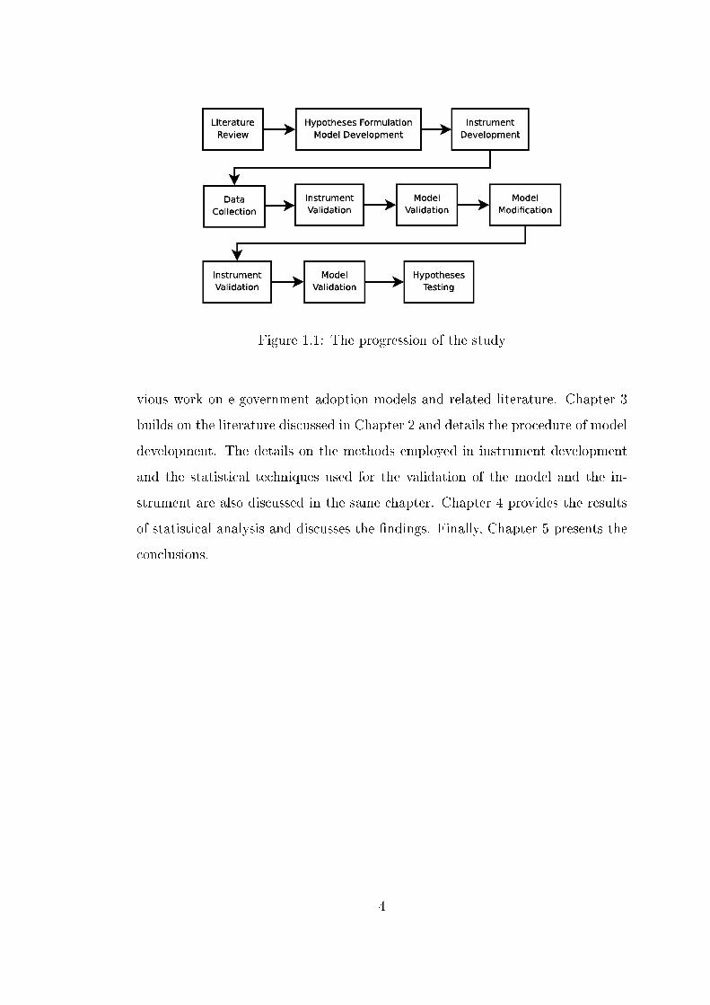
Figure 1.1: The progression of the study

vious work on e-government adoption models and related literature. Chapter 3

builds on the literature discussed in Chapter 2 and details the procedure of model

development. The details on the methods employed in instrument development

and the statistical techniques used for the validation of the model and the in-

strument are also discussed in the same chapter. Chapter 4 provides the results

of statistical analysis and discusses the �ndings. Finally, Chapter 5 presents the

conclusions.

4

CHAPTER 2

LITERATURE REVIEW

This chapter puts forth the previous work done in the literature on the e-government

adoption and on related �elds. Section 2.1 provides an overview of adoption mod-

els used both in general and in e-government context. Section 2.2 focuses on trust

construct which had seen wide employment in e-government studies. Section 2.3

gives an insight into local factors that might a�ect the citizens' adoption behav-

ior. Finally, Section 2.4 discusses an alternative to the general trend in technology

adoption models which is also adopted in this study and provides insight into the-

ory of planned behavior (TPB).

2.1 Adoption Models

There are various models for the adoption of technological novelties in the lit-

erature. Most common of these general models are discussed in Section 2.1.1.

For speci�c technologies or implementations of novelties, such as e-commerce or

e-government, these models are generally taken as a base and extended using

various constructs that are deemed relevant to the subject. E-government adop-

tion literature has also followed a similar path. Section 2.1.2 discusses previous

literature on e-government adoption.

5

2.1.1 General Models

These general models are often referred to as technology adoption models. Per-

haps the most widely known is the Technology Adoption Model (TAM) [1], yet

other models have seen acceptance in IS domain such as Di�usion of Innovations

(DOI) [2] and Uniform Theory of Acceptance and Use of Technology (UTAUT)

[3].

An evaluation of these models reveals that, similar constructs can be observed

in each model, under di�erent names. Most prevalent of these constructs are the

usability 1 and the functionality 2. These constructs also consistently showed

strong e�ects on intention to use and actual use in the broadest set of contexts.

Technology Adoption Model

Davis' seminal work the Technology Acceptance Model is known as the only

commonly accepted theory in IS domain [13]. Despite its prevalence in IS domain,

TAM takes its roots from a theory in psychology; Theory of Reasoned Action

(TRA) [14]. TRA is a theory that explains human behavior. Davis took TRA

and modi�ed it to explain the technology adoption behavior. According to Davis,

adoption of an IT artifact depends on two basic constructs; Perceived Usefulness

(PU) and Perceived Ease of Use (PEU). Perceived usefulness is the perception of

additional performance gained by the use of the system in question. Perceived

ease of use is the perceived reduction in the e�ort required to carry out the task

by using the system in question. Perceived usefulness and perceived ease of use

determine the intention to use the system which in turn has an e�ect on the

actual system use. It has been found later on, that perceived ease of use was also

an antecedent of perceived usefulness and was partially mediated over the later

[1]. In all the years since its conception in 1986 it has been validated time and

1Perceived ease of use of TAM [1], technical complexity of DOI [2], e�ort expectancy of

UTAUT [3]2Perceived usefulness of TAM [1], relative advantage of DOI [2], performance expectancy of

UTAUT [3]

6

again almost to certainty [13].

Figure 2.1: Technology Acceptance Model [1]

Di�usion of Innovations

Di�usion of innovations theory stems from sociology and was not initially con-

ceived as a model for technology adoption but as a model for innovation in general.

Moore and Benbasat carried the theory over to the the IS domain and expanded it

to include eight independent constructs: voluntariness, relative advantage, com-

patibility, image, ease of use, result demonstrability, visibility, and trialability [2].

This model is a direct model3. This makes the model suitable for testing with

�rst generation multivariate analysis techniques. Even though the model o�ers

a comprehensive set of constructs, later work found out that the factors consis-

tently came up in DOI studies were technical compatibility, technical complexity,

and relative advantage [15].

Uniform Theory of Acceptance and Use of Technology

Venkatesh and others reviewed and empirically compared the existent literature

on IT adoption and formulated the Uniform Theory of Acceptance and Use of

Technology [3]. The resulting model included Performance Expectancy, E�ort

3No mediating latent variables in the model.

7

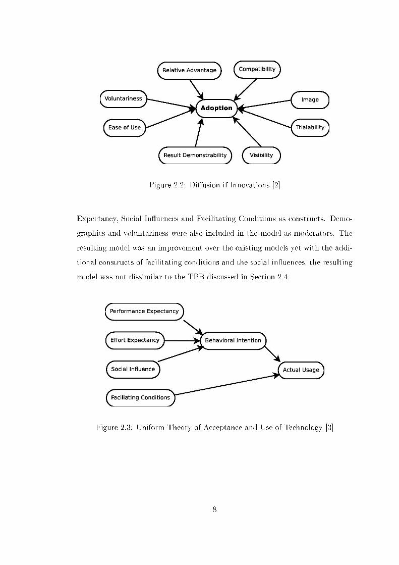
Figure 2.2: Di�usion if Innovations [2]

Expectancy, Social In�uences and Facilitating Conditions as constructs. Demo-

graphics and voluntariness were also included in the model as moderators. The

resulting model was an improvement over the existing models yet with the addi-

tional constructs of facilitating conditions and the social in�uences, the resulting

model was not dissimilar to the TPB discussed in Section 2.4.

Figure 2.3: Uniform Theory of Acceptance and Use of Technology [3]

8

2.1.2 E-government Adoption Models

The models developed for e-government adoption are generally based on one of the

models listed in Section 2.1.1. This is quite logical, considering that e-government

is itself a technology artifact. These models usually extend the technology adop-

tion models by the inclusion of various additional constructs to account for the

multi disciplinary nature of the �eld. Due to the close relations between the �elds

and the relative maturity of e-commerce literature, the studies in e-government

adoption have been known to follow the studies in e-commerce [16, 17]. Even

though the e-commerce literature is not discussed openly in this section, the re-

semblances are pointed out with references given to e-commerce articles in the

following sections.

Table 2.1 lists some e-government adoption studies, the models used as the

basis and the additional constructs included in those studies. The articles listed

in Table 2.1 were chosen to re�ect some trends in the literature. A brief review

of the literature on e-government adoption reveals that TAM was the model that

was utilized most often in the literature [13]. Trust has also seen frequent use in

many studies regarding e-government adoption. This is also true for e-commerce

[10, 18, 19]. The frequent use of trust is probably due to its being a salient factor

in online interractions.

[16], [22] and [23] were notable since their move away from TAM re�ects a

recent trend in IS. DOI, UTAUT and TPB have been employed in its stead. This

trend will be discussed in detail in Section 2.4.

[11] displayed an interesting e�ort into a cross cultural study on e-government.

Skills and Access �discussed in more detail in Section 2.3� were integrated into

TAM to re�ect a country's position in digital divide. Using the information

and communication technology penetration for comparison among two countries

provided a tangible and easily employable measure of local di�erences.

[16] integrated TAM constructs and Trust into DOI. Unfortunately DOI al-

ready had constructs similar to TAM constructs (relative advantage and ease of

9

Table 2.1: Base Models and Additional Constructs in Previous Studies

Study Base Model Additional constructs

Carter and Belanger, 2005 [16] DOI PU, PEU, Trust

Carter and Weerakkody, 2008 [11] TAM Trust, Skills and Access

Gefen et. al., 2002 [20] TAM Social In�uence, Trust and Risk

Warkentin et. al., 2002 [21] TAM Trust, Risk, PBC

AlAwadhi and Morris, 2008 [22] UTAUT -

Hung et. al., 2006 [23]

PU, PEU, Risk,

Trust, Personal Innovativeness,

D-TPB Compatibility, External In�uence,

Interpersonal In�uence, Self-

E�cacy, Facilitating Conditions

use) and the constructs overloaded each other out. The end result was simply

DOI extended by trust. This study exempli�es how disregarding the theoretical

foundations of constructs in a model distorts the results. [24] warns against such

implementations.

[21] extended the TAM with PBC, trust and risk. The use of PBC is notable

since it is in an e�ort to upgrade TAM's basis from TRA to TPB. The end result

was similar to UTAUT with social in�uence construct replaced by trust and risk.

[23] used the decomposed variant of TPB and integrated DOI constructs trust

and risk into the model an approach similar to the one adopted in this study and

[19]. The total number of constructs however rendered the path strengths of con-

structs rather weak and the �nal model reached through the use of modi�cation

indices did not have any theoretical support to the relations investigated and did

not resemble TPB in anyway.

Returning back to factors in�uencing e-government success listed by the UN

report discussed in Chapter 1, it can be seen that the additional constructs in

these models cover a signi�cant amount of them. Usefulness and access ibility,

10

being the most basic determinants of technology adoption had been investigated

in all of the studies. Lack of trust and con�dentiality had been investigated in

studies [16, 11, 20, 21, 23]. The infrastrucute, and service delivery had been

investigated in [11].

2.2 Trust

As exempli�ed in the Section 2.1.2 trust is the most common construct that is

integrated into the e-government adoption models. Trust eases the transactions

in uncertain situations by reducing the perceived complexity of the situation [18].

The level of uncertainty in on-line interactions has made trust a signi�cant factor

for both e-commerce [9] and e-government [25] adoption studies. The literature

provides various descriptions and approaches to trust none of which is agreed

upon [9, 10].

There are two approaches in de�ning trust: de�ning trust as a unitary concept

or as a combination of several concepts. Rotter represents the classical approach

by de�ning trust as a unitary concept [26]. According to Rotter trust is the

expectancy that the word of the trustee is reliable. While Rotter's work is still

used (see [16, 11]), the concept of trust as a unitary construct has long been

debated [9]. Both [9] and [10] discussed below exemplify the approach to trust as

a combined construct.

De�ned whether as a unitary concept or a combination of concepts, trust

has several di�erent types. One point of distinction is the distinction based on

context. The e�ect of the environment and situation in which the transaction

takes place is named institutional trust whereas the e�ect of trustee is named as

party based trust.

McKnight et. al. conducted a study based on TRA [9]. They reviewed litera-

ture and identi�ed �fteen beliefs relating to trust. Eleven of these beliefs clustered

under three major trusting beliefs, integrity, benevolence and competence. The

approach in their work is an example of de�ning trust as a combined construct

11

and is suitable for party based trust.

Institutional trust used in on-line interactions is another example of trust as

a combined construct. The institutional trust re�ects the trust caused by the

situational normality and structural assurances. Situational normality refers to

the feeling of trust stemming from the perception that everything operates as it

should. Structural assurances on the other hand refer to the guarantees and legal

recourse that make the environment more reliable [10].

Risk comes to mind as a natural extension to trust, yet studies could not

arrive at consistent results on the e�ect of risk (see [18, 25]). The direction of the

relation between trust and risk is also controversial. These two constructs may

mediate each others' e�ects.

2.3 Local Factors

Re�ecting on the international nature of the e-government phenomena, there are

inter-cultural comparison studies. The models aiming for inter-cultural compari-

son generally include constructs to account for the local factors [27, 11]. Although

there are well known examples of inter-cultural research such as Hoefstede's cul-

tural dimensions or Schwartz's value inventory [28], the integration of these into

a measurement instrument is hard and the results obtained from previous stud-

ies based on these might not be compatible with the sample at hand. Thus a

more measurable and tangible scale to account for di�erences among countries

was needed. This led Carter and Weerakkody to use IT penetration to compare

UK and US [11]. Carter and Weerakkody theorized that the countries' position

in digital divide e�ects the IT penetration which in turn e�ects the citizens' abil-

ity to use computers and the availability of computers. Yet, in cases where IT

penetration is too deep, the IT artifacts and their e�ects might become invisible

[11]. The citizens' computer skills and access to computers are easily measurable

and are tangible measures.

Even though Carter and Weerakkody used these measures for inter-cultural

12

comparison, these measures were more general in nature and di�ered even among

the members of di�erent social strata in the same country. The true marvel of IT

penetration evidenced by the social capital and the infrastructural adequacy was

that it was an indicator of local factors and enabler of the use of e-government

services.

2.4 Theory of Planned Behavior as an Alternative

While TAM has seen wide acceptance and use in information systems literature,

its dominion has not been without resistance. Benbasat and Barki have noted

the limitations of TAM in terms of extendibility and explanatory power [13]. The

argument against the explanatory power arose from the overly simplistic structure

of the model. Many researchers have proven that -as Benbasat and Barki put it

- �usefulness was useful� in a�ecting intentions, but TAM did not provide any

insights into what usefulness was nor provided any mechanism to do so later

on if the researcher wished. This formed the basis for the second argument

against TAM, the extendibility. TAM did not include any extension facilities

and the researchers aiming to extend the model needed to justify this in terms

of TAM. Over the years, as the limitations of TAM became clear, researchers

either extended the existing model or moved to other models such as UTAUT

or DOI for the explanatory power. While it is true that these models do have

more explanatory power, they too do not provide default extension mechanisms.

As noted in [13] UTAUT was very similar to the Theory of Planned behavior

with the inclusion of social in�uence (subjective norms in TPB) and facilitating

conditions (perceived behavioral control -PBC- in TPB) but lacked the salient

belief mechanism of extension. Remembering that TAM was based on TRA - the

antecedent of TPB - Benbasat and Barki suggested using TPB instead of other

models for the sake of the extendibility. This study adopted that approach and

used TPB as the base of the model developed.

Theory of Planned Behavior is a theory in social psychology, explaining hu-

13

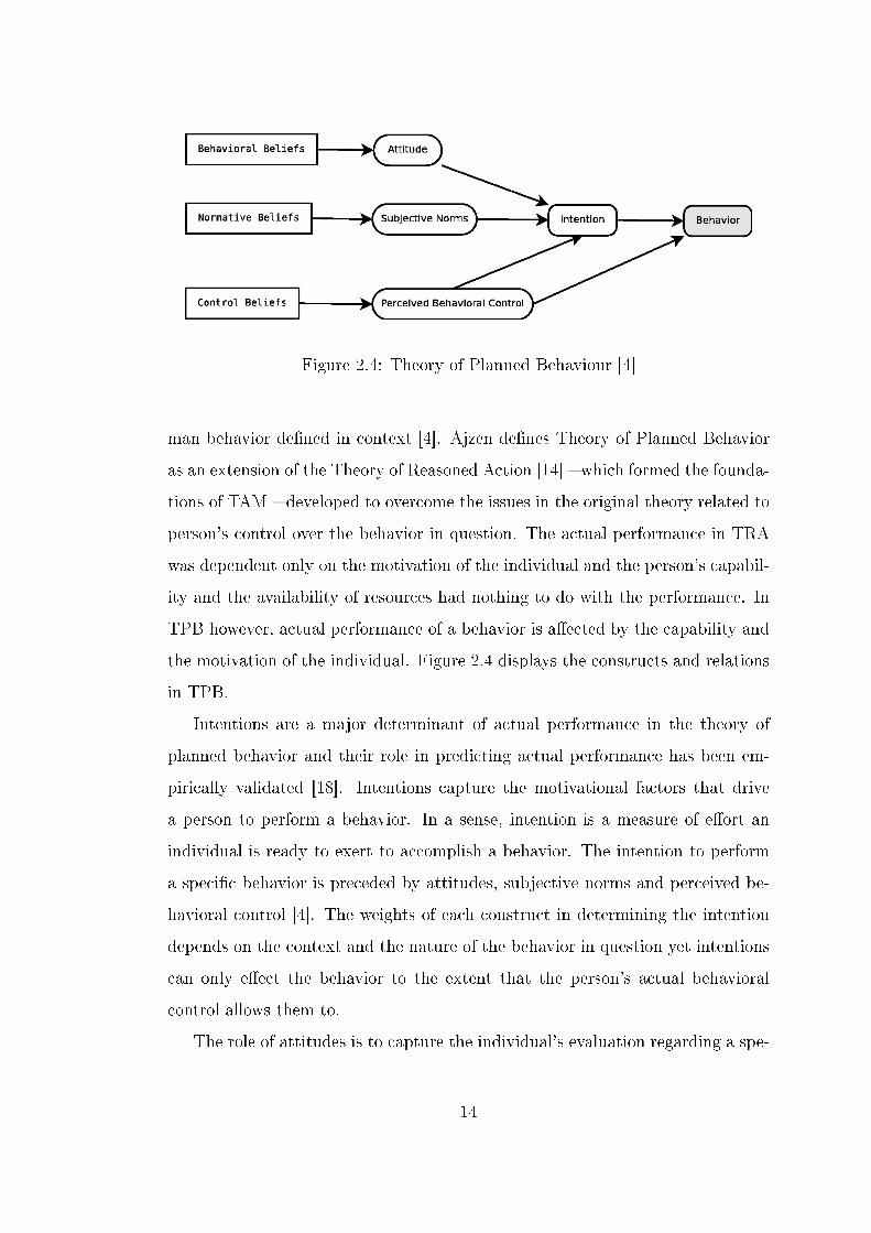
Figure 2.4: Theory of Planned Behaviour [4]

man behavior de�ned in context [4]. Ajzen de�nes Theory of Planned Behavior

as an extension of the Theory of Reasoned Action [14] � which formed the founda-

tions of TAM � developed to overcome the issues in the original theory related to

person's control over the behavior in question. The actual performance in TRA

was dependent only on the motivation of the individual and the person's capabil-

ity and the availability of resources had nothing to do with the performance. In

TPB however, actual performance of a behavior is a�ected by the capability and

the motivation of the individual. Figure 2.4 displays the constructs and relations

in TPB.

Intentions are a major determinant of actual performance in the theory of

planned behavior and their role in predicting actual performance has been em-

pirically validated [18]. Intentions capture the motivational factors that drive

a person to perform a behavior. In a sense, intention is a measure of e�ort an

individual is ready to exert to accomplish a behavior. The intention to perform

a speci�c behavior is preceded by attitudes, subjective norms and perceived be-

havioral control [4]. The weights of each construct in determining the intention

depends on the context and the nature of the behavior in question yet intentions

can only e�ect the behavior to the extent that the person's actual behavioral

control allows them to.

The role of attitudes is to capture the individual's evaluation regarding a spe-

14

ci�c behavior whereas subjective norms capture the social pressure on performing

or not performing the behavior. The attitudes have been proven to in�uence the

intentions. Subjective norms however have played a controversial role in online

settings. Venkatesh et. al. found social norms to be signi�cant (and slightly at

that) only in mandatory settings or for the initial use of the system where the

experience is low [3].

Availability of resources and opportunities � actual behavioral control � re-

quired to perform the speci�ed behavior dictate the actual performance to the

extent that the person in question is motivated to try. Perceived behavioral

control � the di�erentiating point of TPB � measures the perceived di�culty of

performing a speci�c behavior. Ajzen likens his PBC construct to Bandura's

self-e�cacy construct [4]. Yet in time studies managed to identify another fac-

tor determining the PBC, controllability. Perceptions of self-e�cacy related to

the individuals' judgments of their abilities where as controllability refers to the

individuals' judgments of the availability of resources. Ajzen answered claims

against the unitary nature of PBC by stating that even though PBC is composed

of separable components it is still a unitary construct [12]. According to the same

article, both self-e�cacy and controllability belief items must be included in PBC

measures. In TPB, PBC e�ects the performance both directly and through inten-

tions, but the size of the direct e�ect is proportional to the compatibility between

perceived and actual control.

The constructs detailed so far �Intentions, Attitudes, Subjective Norms and

Perceived Behavioral Control� su�ce for the prediction of behavior. Thus, they

are called the predictor variables4.

The explanatory power of the model stems from the inclusion of salient beliefs

into the model. The salient beliefs provide the researchers with the ability to

4The parts making up a model are generally referred to as constructs. However Ajzen called

these, variables. Moreover, in SEM literature they are generally referred to as latent variables.

Throughout this text, construct, variable and latent variable have been used interchangeably

based on the context

15

investigate the relevant factors and their e�ects on the behavior. Three types of

these salient beliefs each pertaining to a higher level construct exist; behavioral

beliefs which in�uence attitudes, normative beliefs which in�uence the subjective

norms and control beliefs which in�uence the perceived behavioral control [4].

The salient beliefs consist of belief composites. The belief composites have a dual

nature; each belief composite is a factor of the subjective probability and the

subjective impact of the belief they are measuring. So, for a belief composite item

in a TPB questionnaire, two questions are asked: the probability of occurrence

and the impact. For the behavioral beliefs the probability of occurrence is the

belief strength and the impact is outcome evaluation. In control beliefs these are

translated into control belief strength and control belief power.

This chapter has discussed the previous work done in technology adoption mod-

els, e-government adoption models and the model used as a base for the model

developed in this study. Chapter 3 details the development of the model proposed

in this study, the measurement instrument and the statistical tools used for the

validation of both.

16

CHAPTER 3

RESEARCH METHODOLOGY

The aim of this chapter is to communicate the theory behind the model developed

and the methods and procedures employed in this study. Section 3.1 elaborates

the basic hypotheses and the theoretical foundations of the model developed. The

processes and methods regarding development of the measurement instrument are

discussed in Section 3.2. Finally Section 3.3 introduces the statistical methods

used to analyze the data gathered in this study.

3.1 Model Development

Due to the reasons discussed in Section 2.4, the use of TPB as a base model

was decided. The model proposed in this study is an extension of TPB into

the e-government setting. The constructs, perceived usefulness, perceived ease of

use, trust in internet, trust in government, skills and access are integrated as

salient beliefs. The linkages among these constructs were provided in the form

of a collection of hypotheses, Figure 3.1 shows the hypothesized relationships.

The actual performance of behavior could not be measured since it required a

longtitutional study with a limited sample. This was not possible due to the time

constraint imposed by the master's process and sample size constraints imposed

by the statistical technique employed. The role of intentions on actual perfor-

17

mance has been reported to be a strong predictor of actual usage [3, 4]. Ajzen

suggested eliciting salient beliefs through a separate survey study, however in or-

der to evaluate the most common constructs in e-government adoption literature

that suggestion is disregarded. No belief types were integrated through subjec-

tive norms construct, since the subjective norms have been known to play a non

signi�cant role in on-line interactions [3].

Figure 3.1: The Proposed Model

3.1.1 Predictor Constructs

The predictor variables1 form the foundations of TPB. The relationships among

these constructs have been taken as they were envisaged by Ajzen [4] and were

provided in the form of the hypotheses below. More information on predictor

variables, their relations and TPB in general can be found in 2.4.

1Intention, attitude, subjective norms, perceived behavioral control

18

H1 † The intention to use an e-government service positively in�uences the actual

usage of the service.

H2a Perceived Behavioral Control over using an e-government service positively

in�uences the intention to use the service.

H2b † Perceived Behavioral Control over using an e-government service posi-

tively in�uences the actual usage of the service.

H3 Attitude towards using an e-government service positively in�uences inten-

tion to use the e-government service.

H4 Subjective norms regarding the use of an e-government service will have a

positive e�ect towards the intention to use the service.

3.1.2 Salient Beliefs

The constructs discussed in this section were integrated into the model as salient

beliefs. The discussion on salient beliefs and their role in TPB can be found in

Section 2.4. The constructs are categorized according to their domain of origin.

Detailed literature on the constructs can be found in Chapter 2.

Technology Acceptance Beliefs

As discussed in Section 2.1.1, functionality and usability have consistently showed

strong e�ects on intentions. Thus functionality and usability were integrated into

the model as perceived usefulness and perceived ease of use.

Perceived Usefulness: In G2C context, perceived usefulness of using an e-

government service is the extent to which a citizen believes, using the e-government

service would enhance her e�ciency. The e�ect of PU on attitude had empirically

been shown by [1]. Hence, the following:

†Due to practical reasons regarding data collection these two hypotheses could not be tested

in this study.

19

H5 Perceived Usefulness of an e-government service will have a positive e�ect on

the attitude toward the use of e-government service.

Perceived Ease of Use: Perceived ease of use in G2C setting, pertains to how

much a citizen believes the use of an e-government service will be free of e�ort.

[1] has shown that PEU in�uenced intentions over attitudes. Based on this, the

following is proposed:

H6a Perceived Ease of Use of an e-government service will have a positive e�ect

on the attitude toward the use of e-government service.

Bandura's self e�cacy forms the basis of both PBC in TPB [4] and PEU in

TAM [1], therefore the two constructs are theoretically connected. In other words,

both constructs relate to a reduction in the amount of e�ort required. Thus the

following was proposed:

H6b Perceived Ease of Use of an e-government service will have a positive e�ect

on the perceived behavioral control of the e-government service.

Trust Beliefs

Party Based Trust: The party based trust in G2C setting refers to trust in the

government institution providing the e-government service. This construct is

referred to as Trust in Government (TG) [11]. Trust plays a role in the attitudes

of the citizens by enhancing their expectations of the outcomes. [14] formulates

attitudes as a factor of outcome expectations and outcome values. Thus by

manipulating expectations it is possible to manipulate attitudes. The role of

party based trust on attitudes has been empirically shown in [19] for e-commerce

setting.

H7a Trust in government will have a positive e�ect on the attitude toward the

use of e-government service.

20

Trust has generally been known to reduce the perceived complexity of a trans-

action [10]. The reduced complexity could translate into increased perceived

control over the situation.

H7b Trust in government will have a positive e�ect on the perceived behavioral

control of using an e-government service.

Institutional Trust: Institutional trust refers to a perception of safety caused

by the environmental conditions � structural assurances and situational normality

� surrounding the transaction. The environment in which the transactions take

place in G2C settings is generally the internet. Thus this construct was named

Trust in Internet. The proposed hypothesis for trust in government were based

on the nature of trust itself and are expected to hold for trust in internet also.

H8a Trust in internet will have a positive e�ect on the attitude toward the use

of e-government service.

H8b Trust in internet will have a positive e�ect on the perceived behavioral

control of using an e-government service.

Beliefs on Local Factors

Skills: Skills construct refers to the ability of a person to use technology. As

laid out in [24], the perceived behavioral control construct is a unitary construct

combining self e�cacy and locus of control. Beliefs of a citizen regarding her

abilities to use a technology, directly relates to the self-e�cacy and should have

an e�ect on PBC.

H9 Having the skills to use a computer will have a positive e�ect on the perceived

behavioral control of an e-government service.

Access: Access construct refers to how easily a person can access technology.

Beliefs of a citizen regarding his capacity to access technology, directly relates to

the locus of control and should have an e�ect on PBC.

21

H10 Having access to computers will have a positive e�ect on the perceived

behavioral control of an e-government service.

3.2 The Setting of the Study and Instrument De-

velopment

The student loans service of "higher education student loans and accomodation

association" (KYK) was chosen to validate the model. This service was a G2C

service geared towards students. This decision was based on the readily avail-

able student sample at hand. KYK is the governmental body responsible for

the dormitory accommodation and student loans provided by the government in

Turkey. The association provides several services related to its �eld. In order to

to narrow down the scope, only the loan services were investigated. Two types of

loans are provided by the association, one paying part of the tuition fee and the

other as a direct contribution to the student herself. The students can access loan

announcements, inquire on their loan id's, payment and payback details through

the KYK website.

Ajzen, being disturbed by the �aws in the implementations of his theory in

the literature wrote a guideline on the TPB instrument development [24]. In this

study, the measurement instrument was developed in accordance with Ajzen's

suggestions. The measures employed in this study were drawn from the literature

and adopted into the study to �t the context of the study and the requirements

of TPB. Table 3.1 shows the sources for items included in the study. Items for

predictor variables2 were adopted from [12]. Items for technology acceptance were

adopted from [1], the trust items were adopted from [9] and local factors items

were adopted from [11].

Ajzen points out that arbitrarily combining items from various studies might

harm the internal consistency of the model. To prevent this, the compatibility

2Intention, attitude, subjective norms, perceived behavioral control

22

Table 3.1: Items Used in Instrument and Their Sources

Measurement Items SOURCE

Predictor Variables Ajzen, 2002 [12]

Technology Acceptance Davis, 1989 [1]

Trust McKnight et. al., 2002 [9]

Local Factors Carter and Weerakkody, 2008 [11]

of the items in the study was ensured by structuring them to re�ect a speci�c

behavior de�ned in terms of Target, Action, Time and Context (TACT) as sug-

gested by Ajzen. The behavior in question in our study was de�ned as: �Using

the kyk.gov.tr web page to get loan payment details during the semester�. All

predictor variable items were rewritten to re�ect this behavior. Since the items

for salient beliefs were to be integrated into the model as belief composites they

had to be rewritten to be compatible with TPB belief composites. This required

writing two separate questions for each item, one measuring the likelihood and

the other measuring the impact of the occurrence described by the item, as dis-

cussed in Section 2.4. In accordance with Ajzen's guidelines, two separate trust

measures were developed for each trust belief, one for behavioral beliefs and one

for control [24].

Five point likert scales were employed for all items, with 1 denoting a negative

answer and 5 a positive answer. The items were presented to the respondents

in random order to reduce the e�ects of method halo [29]. The questionnaire

also collected basic demographic data through 5 questions. The resulting items

were reviewed to ensure that the meaning was preserved through adoption and

translation to Turkish. In the end of the instrument development, a total of

81 questions, including the demographic items, were in the �rst version of the

questionnaire. As suggested in [24, 30], multiple questions for each variable were

developed which were then re�ned through the pilot study.

Apart from the questionnaire, the instrument also included a familiarization

23

task. The familiarization task was only applied to respondents without prior

experience with the KYK web site to acquaint these users with the site. The task

consisted of simple discovery tasks to familiarize the user to KYK and e-services

provided by KYK and detailed descriptions of each key e-services. The �nal state

of the instrument can be found in the Appendix Appendix C:.

Since our research involved human participation for the data collection phase

the approval of the Practical Ethics Research Board at the Middle East Technical

University has been taken (See Appendix Appendix B:))

3.3 Data Collection and Analysis

This section details the methods used for data collection and analysis.

3.3.1 Pilot Study

A pilot study was conducted to test and re�ne the measurement instrument on a

convenience sample of �fty people and thirty-two valid responses were acquired

(response rate 64%). The pilot data was analyzed to see if there was any di�erence

between the respondents that had previous experience with the system and the

ones that had not. Welch's two sample T-test was used with a con�dence interval

of ninety-�ve percent on all items in the scale. None of the items showed a

statistically signi�cant di�erence, so the two samples were statistically the same.

This meant that the responses from people with no prior experience with the

system could be used in analysis.

Cronbach's alpha was calculated for the questionnaire items to test the inter-

nal consistency of the items measuring the same construct. According to [31] a

factor loading between seventy to eighty percent, points to a good internal con-

sistency whereas a loading above eighty percent indicates an excellent internal

consistency. The α tests revealed that all constructs except for one had alpha

values above seventy percent, revealing that all constructs had good internal con-

24

sistency. The instrument was re�ned to increase the α values, after which nine

items were removed from the instrument.

Factorial validity could not be assessed at pilot study stage because of the

sample size requirements [32].

The questionnaire was altered to eliminate any possible misunderstandings

due to wording. Description of some tasks and minor wording details in survey

items have been altered according to the feedback from the subjects. The items

reducing the α value of their constructs were also removed, leaving 63 questions

in the questionnaire.

3.3.2 Data Collection

The altered instrument was administered to 392 people on-line over a period of

two months. The sample consisted of under-graduate, graduate students and

university graduates � the target audience of the KYK web services. The in-

strument was administered seperately to the graduate students and the rest via

di�erent medium. For the graduate students, the instrument was �lled as part of

their class activirty. The respondents were not given any credits for this and the

participation was voluntary. The rest of the participants received the instrument

through facebook social networking application. Average response rate was 55.1%

and a total of 216 valid responses were returned. Out of 216 respondents 145 were

female, 71 male. The age of respondents ranged from 18 to 32 with a mean of

22.47 and a median age of 21. 32% of the respondents reported an average daily

internet use of 1-3 hours, followed by 25% with a daily internet use of 7 hours or

more. 32% of the respondents reported that they did not use any services over

the internet whereas 53% reported that they used internet to use e-government

services. Of the 216 respondents 65% reported previous use of the KYK services.

25

3.3.3 Data Analysis

Among the various methods of analysis, the second generation multivariate tools

(SEM, PLS-PM) are steadily becoming the norm in IS. Gefen et. al. conducted

a review of articles published in the three major journals of IS domain and con-

cluded that the use of second generation techniques had been increasing since

1990's [33]. This is due to some clear advantages second generation techniques

hold over the �rst generation techniques (multiple regression, PCA, cluster anal-

ysis). These advantages can be listed as:

• Previous knowledge can be incorporated into the analysis for con�rmatory

purposes.

• Unobservable constructs and abstract concepts can be modeled

• Measurement errors can be accounted for in the model.

The best part is that all these can be done in a single run of the analysis (in

contrast to multiple runs in multiple regressions analysis). The model developed

in this study is based on abstract constructs based on prior theory, furthermore

these constructs are interlinked - making the �rst generation tools impractical.

Thus the use of these second generation multivariate tools was most appropriate

for the model at hand.

Structural Equation Modeling Procedure and Requirements

A brief introduction to the second generation multivariate tools and their re-

quirements have been made in this section. The second generation multivariate

tools generally go under the name of Structural Equation Modelling (SEM). SEM

analysis is described as a cross between factorial analysis and path analysis be-

cause it is based on two models. A measurement model � akin to con�rmatory

factor analysis (CFA) � with manifest variables3 (MV) is used to estimate latent

3The items in a questionnaire for example.

26

variables4 (LV) which in turn will be used in the structural model to estimate the

relations among these LVs � the path analysis [32].

There are two types of SEM, covariance based and partial least squares (PLS)

based SEM, both of which can currently be carried out in R statistical computing

environment [34]. Covariance based SEM with maximum likelihood (ML) estima-

tion can be carried out by the sem package [35] and PLS based SEM can be carried

out by pls-pm package [36]. The covariance based SEM provides results general-

izable to the population whereas the results of PLS based SEM �also referred to

as PLS path modelling (PLS-PM)� are more geared towards making predictions

based on the data. The values for paths can be �xed in covariance based SEM

whereas PLS-PM provides no such functionality. Despite its statistical powers,

the covariance based SEM is also more stringent in comparison to PLS-PM in

terms of requirements. A typical SEM analysis is generally conducted in seven

steps [32] and each step comes with several unique requirements that have to be

met.

The �rst step in SEM analysis is the model speci�cation. The model is spec-

i�ed by formulating the hypothesized relations based on previous theories. This

step is carried out in section 3.1 of this study. It is crucial to base the analysis

on the previous theory due to the con�rmatory nature of the technique. The

relationships in SEM do not imply causality, and without theoretical support no

inferences can be made about the relations. A model can be represented either as

a list of equations or a path diagram but the path diagram is generally preferred

due to the communicative power. A simple SEM path diagram can be seen in Fig-

ure 3.2. The LVs are generally depicted in the path diagrams as circles or ellipses

whereas the MVs are depicted as squares or rectangles. Arrows indicate relations

among these variables but these relations do not necessarily imply causality. The

arrows tagged with β form the structural model whereas the arrows tagged with

λ form the measurement model. The direction of arrows in the measurement

model indicate the type of relationship between MVs and LV. If the arrows in the

4Abstract concepts such as emotions, which are not directly measurable.

27

measurement model originate from LV, then the MVs are said to be re�ective �

re�ecting upon the e�ects of a common factor � else, the MVs are formative �

forming a common factor.

Figure 3.2: A Simple SEM Path Diagram

Second step in covariance based SEM is the model identi�cation. For a model

to be analyzable, it shall be over-identi�ed [30]. A model is over-identi�ed when

the data provides more information then the information being estimated. In

practical terms, the number of data items5 must be higher than the number

of parameters to be estimated6 [32]. Having at least three MVs for each LV is a

useful heuristic to ensure model identi�cation [30]. Models in PLS-PM are always

identi�ed and model identi�cation is not an issue in PLS-PM.

Third step is related to the data requirements. Structure of data, sample size,

multicollinearity, normality, missing data are all factors in SEM.

Sample size requirements vary according to the type of SEM analysis to be

implemented. The sample size requirements for covariance based SEM are also

much higher in comparison to PLS based SEM. That is the reason why PLS-PM

is referred to as poor man's SEM. Recommended sample size for covariance based

5The number of correlations in the correlation matrix6Error variances and factor loadings, etc.

28

SEM is 10-20 observations per parameter to be estimated, with a bare minimum

of 150 cases whereas PLS-PM requires only 10 observations per parameters to be

estimated in the most complex construct alone with a recommended minimum of

45 [33]. PLS-PM with sample sizes as low as 6 has been used in the literature

[37].

Multicollinearity disrupts both methods. Strong correlations (>.85) among

items cause redundancy and as a result unreliable path loadings [32]. While not

e�ecting the overall �t or the prediction power of a model, multi-collinearity might

blur the relationships among constructs. This issue can be lessened in PLS-PM

through the use of PLS regression on the prediction of path coe�cients [37].

ML estimation, the defacto standard in covariance based SEM, is known to

be problematic with non-normal data [33, 32]. The data must be multivariate

normal for SEM using ML estimation whereas PLS based SEM is known to be

more robust against deviations from normality.

The covariance and correlation matrices used in both types of SEM cannot

be computed in the existence of missing data. The missing data should either be

removed or imputed before the analysis.

The fourth step is the estimation of the model using the statistical software.

The type of estimator (ML, LS, PLS, ULS, etc...) to used is based on the whether

the structure of the data was normal or non-normal. At this step, the measure-

ment model is analyzed with CFA with the chosen method of estimation to ensure

factorial validity7 of the model and proper adjustments are made to the measure-

ment model to increase factorial validity. Some researchers also suggested using

EFA for a deeper understanding of data structure [38].

Fifth step is to review the model �t and interpret the results. The model is

reviewed to ensure the strength of path loadings are satisfactory, the predictive

power of the model is strong and the �t indice for the overall model is good.

Unfortunately, the goodness of �t indices (GFI) are not as common in PLS-PM

7The items load together highly only on the factor proposed, a combination of convergent

and discriminant validity.

29

as in covariance based SEM but when all MV are taken as re�ective a GFI can

be used.

Sixth step is to modify the model to increase the model �t, path coe�cients

and explanatory power. Some researchers argue against this on the basis of loosing

theoretical support. If the modi�cation indices are followed blindly, disregarding

previous theory, this might lead to conclusions that are speci�c to data at hand.

Thus in this stage any modi�cations shall be �rmly supported by theory.

Seventh step is comparison of alternate models. The alternate models based on

plausible theory are tested and compared to the proposed model. The strength

and signi�cance of paths, the total variance explained by each model and the

goodness of �t indices are compared.

The results of statistical methods discussed in this chapter are provided in Chap-

ter 4.

30

CHAPTER 4

RESULTS AND DISCUSSION

This chapter presents the results and discussion of the statistical analyses con-

ducted on the data. The seven step SEM procedure discussed in Section 3.3.3

has been followed in analyzing the data. The model speci�cation step had been

carried out in 3.1 and the use of PLS-PM removed the necessity of model-

identi�cation. Section 4.1 contains the analyses conducted to ascertain if the

data met the requirements of SEM and continues the SEM conduct from step

three. The actual results of estimation was provided in Section 4.2. The modi�-

cations to the model and the estimation of the parameters of this new model are

discussed in Section 4.3 and Section 4.4. The comparison of alternate models had

been carried out in Section 4.4.4. The �nal section of this chapter (Section 4.5)

sums up the �nal model and discusses the results. Model identi�cation step is

skipped since the data discussed in Section 4.1 was unsuitable for covariance

based variation of SEM.

4.1 General Properties of the Data

After the data collection stage the data was imported into R statistical computa-

tion environment [34] for analysis. The �rst step was to remove the outliers since

outliers are known to have serious adverse e�ects in SEM [32]. The detection of

31

outliers was carried out as follows: a script written by the author detected cases

where all items had the same value. This process revealed four outliers which

were removed from the dataset.

Skewness =

√n× (n− 1)

n− 2

× m3

m322

(Equation 4.1)

Kurtosis =

[(n− 1)(n+ 1)

(n− 2)(n− 3)

]× m4

m22

− 3

[(n− 1)2

(n− 2)(n− 3)

](Equation 4.2)

Figure 4.1: Formulas for calculation of critical values for skewness and kurtosis

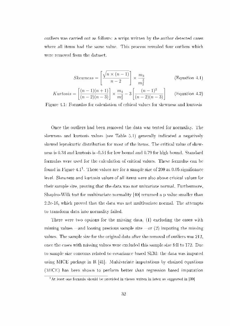
Once the outliers had been removed the data was tested for normality. The

skewness and kurtosis values (see Table 5.1) generally indicated a negatively

skewed leptokurtic distribution for most of the items. The critical value of skew-

ness is 0.34 and kurtosis is -0.54 for low bound and 0.79 for high bound. Standard

formulas were used for the calculation of critical values. These formulas can be

found in Figure 4.11. These values are for a sample size of 200 at 0.05 signi�cance

level. Skewness and kurtosis values of all items were also above critical values for

their sample size, proving that the data was not univariate normal. Furthermore,

Shapiro-Wilk test for multivariate normality [40] returned a p value smaller than

2.2e-16, which proved that the data was not multivariate normal. The attempts

to transform data into normality failed.

There were two options for the missing data, (1) excluding the cases with

missing values � and loosing precious sample size � or (2) imputing the missing

values. The sample size for the original data after the removal of outliers was 212,

once the cases with missing values were excluded this sample size fell to 172. Due

to sample size concerns related to covariance based SEM; the data was imputed

using MICE package in R [41]. Multivariate imputations by chained equations

(MICE) has been shown to perform better than regression based imputation

1At least one formula should be provided in theses writen in latex as suggested in [39]

32

methods in [42]. T-test values for bootstrap samples indicated that imputed and

missing values excluded data was not statistically di�erent. We ran all the tests

including SEM analysis on both imputed and missing values removed data.

The correlations among items and constructs were inspected to check for

multi-collinearity. As suggested in [43, 44] the correlation matrix of the raw

data is provided in Appendix Appendix F:. Upon inspecting the table, strong

correlations (>.85) were observed among attitude items 1 and 2 and Intention

items 1 and 3. These strong correlations might cause redundancy in the future

steps but are not enough to seriously in�uence the results. The rest of the items

had mild correlations among items of the same measurement group (e.g., among

behavioral belief items, among predictor variable items). It has been infered that

this was due to the method halo caused by the instrument. If the measurement

instrument is inspected, it can be noticed that all the questions share the same

sentence structure. This was due to the suggestions of Ajzen [24]. Ideally the

correlation among the items should only be based on the latent construct that

combines them, yet by formating the sentences to re�ect TACT an additional

correlation due to the sentence structure comes into existence. This is more evi-

dent in the items of the same measurement group since the measurement groups

di�er with each by what they measure. This means the items in a measurement

group shares an even more similar sentence structure, hence the additional corre-

lation. Ajzen probably based his suggestions on the �rst generation multivariate

analysis techniques and never noticed that formating the questionnaire items this

way might give way to multicollinearity. Due to the correlations the path load-

ings in the structural model were blurred. This was more evident in covariance

based SEM implementation2 due to ML estimation scheme. The modi�cations

to the model reduced the e�ects multicollinearity by minimizing the unwanted

correlations.

Exploratory Factor Analysis (EFA) was then applied separately to predictor

2The models were tested with both PLS-PM and covariance based SEM, but only the results

of PLS-PM were provided.

33

variable, behavioral belief and control belief items to gain an overall understand-

ing of the data as suggested in [38] but EFA results were not deemed conclusive

and were further tested by con�rmatory factor analysis (CFA) later on. Even

though Principal Component Analysis (PCA) and EFA had been known to pro-

duce similar results, true factor analysis with varimax rotation was preferred over

PCA because PCA produces higher loadings since it does not separate unique

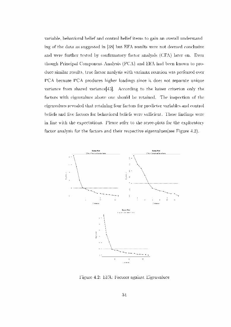
variance from shared variance[45]. According to the kaiser criterion only the

factors with eigenvalues above one should be retained. The inspection of the

eigenvalues revealed that retaining four factors for predictor variables and control

beliefs and �ve factors for behavioral beliefs were su�cient. These �ndings were

in line with the expectations. Please refer to the scree-plots for the exploratory

factor analysis for the factors and their respective eigenvalues(see Figure 4.2).

Figure 4.2: EFA: Factors against Eigenvalues

34

Further inspection of the EFA results were carried out through the factor

loading tables. To ease the understanding, the factor loadings below 0.35 were

not displayed and the loadings of the items to their respective factors are shown in

bold. In general a loading above .60 is considered to be strong whereas loadings as

low as .40 are deemed acceptable. If an item is loading more strongly to a factor

other than the factor it is supposed to load on or if it is loading on multiple

factors equally, then the item is deemed weak [45].

Table 4.1: Factor Loadings for Predictor Variable Items

Items Factor1 Factor2 Factor3 Factor4

INT1 0.77

INT2 0.61

INT3 0.82

INT4 0.56 0.46

ATT1 0.38 0.40 0.62

ATT2 0.43 0.40 0.74

ATT3 0.36 0.66

ATT4 0.66

SN1 0.38 0.36 0.39

SN2 0.49 0.48

SN3 0.47 0.41

SN4 0.71

PBC1 0.75

PBC2 0.63

PBC3 0.65 0.36

PBC4 0.72

The factor loadings for the predictor constructs were mostly in line with the

expectations. As can be seen in Table 4.1 all items except ATT4 had strong

loadings in their respective constructs. The attitude items had a mild cross

35

loading on intention. The subjective norm items were seriously cross loading

to other factors and had low loadings to their factor indicating problems about

factorial validity.

Table 4.2: Factor Loadings for Behavioral Belief Items

Items Factor1 Factor2 Factor3 Factor4 Factor5

bPU1 0.53

bPU2 0.61

bPEU1 0.64

bPEU2 0.78

bTG1 0.65

bTG2 0.77

bTG3 0.60 0.41

bTG4 0.52 0.44 0.38

bTI1 0.62 0.38

bTI2 0.64

bTI3 0.69

bTI4 0.49 0.42

bTI5 0.86

The factor loadings for behavioral belief items can be seen in Table 4.2. The

results again, reveal that the expected factor structure is pretty much achieved.

bTI4 and bTI5 loading into a separate factor is the only evident problem with

factor loadings. Upon the inspection of questionnaire items, these two items were

found to be the situational normality component of institutional trust and have

a di�erent structure than the rest of the items in the construct which accounts

for the problems in factor structure.

Table 4.3 reveals two problems in the factor structure. The �rst problem is

the cross-loading of perceived ease of use items. Like subjective norm items, these

items also have low loading weights on their corresponding factor. The second

36

Table 4.3: Factor Loadings for Control Belief Items

Items Factor1 Factor2 Factor3 Factor4

cPEU1 0.42 0.46 0.44

cPEU2 0.38 0.34 0.72

cPEU3 0.46 0.35 0.53

cTG1 0.69

cTG2 0.36 0.68

cTG3 0.73

cTG4 0.65 0.36

cTG5 0.70

cTI1 0.56 0.42

cTI2 0.38 0.71

cTI3 0.83

cTI4 0.67

cTI5 0.58 0.43

cSK1 0.71

cSK2 0.68 0.35

cACC1 0.76

cACC2 0.76

37

problem is again with the situational normality items cTI4 and CTI5 which load

with local factors instead of institutional trust factor. Except for these two minor

problems, the factor structure is as expected.

4.2 Testing the Initial Model with SEM

Section 4.1 laid out the general properties of the data at hand. According to

the results, the sample sizes were 172 for complete cases and 212 for imputed

data, with non normal distributions, furthermore the correlations among items

while not being particularly alarming, were considerable. Based on the data

requirements of SEM; the use of PLS based SEM was deemed appropriate. The

results of the analysis were validated according to the guidelines laid out in [29].

According to [29] there is an order of precedence among types of validity such that

an instrument must �rst be validated before the internal validity and consequently

statistical conclusion validity can be discussed.

The instrument validity in PLS can be assured through investigation of con-

vergent validity, discriminant validity, internal consistency and unidimensional

reliability [33]. Internal consistency or reliability deals with the accuracy of mea-

surements of an instrument and has traditionally been measured with Cronbach's

α. Ideally a construct should measure one and only one concept, that is the uni-

dimensional validity of the construct. Convergent validity means that the items

theorized to form a construct should have a shared communality � like having

high correlations with one another � whereas discriminant validity means that

the items forming up a construct can be distinguished from items of another

construct � like having low correlations with items of other constructs.

The hypothesized model discussed in Section 3.1 was tested initially, both

with imputed and original data. There were small di�erences between the two

results and since the sample size of 172 of the non imputed data was enough for

PLS-PM analysis the results of non imputed data were provided. All manifest

variables used in this model were re�ective and factorial �tting scheme was used

38

with standardized values in estimations. Please refer to Figure 4.3 for a path

diagram of the proposed relations among constructs.

4.2.1 Instrument Validity

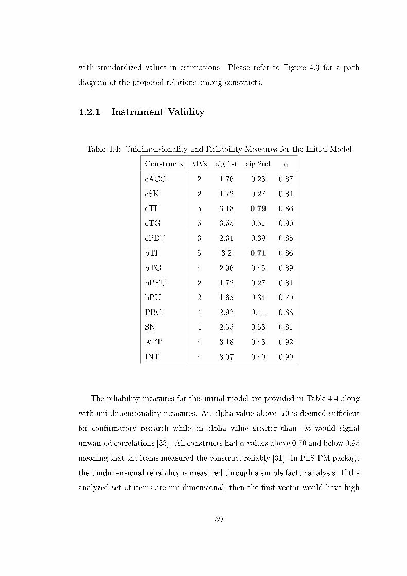
Table 4.4: Unidimensionality and Reliability Measures for the Initial Model

Constructs MVs eig.1st eig.2nd α

cACC 2 1.76 0.23 0.87

cSK 2 1.72 0.27 0.84

cTI 5 3.18 0.79 0.86

cTG 5 3.55 0.51 0.90

cPEU 3 2.31 0.39 0.85

bTI 5 3.2 0.71 0.86

bTG 4 2.96 0.45 0.89

bPEU 2 1.72 0.27 0.84

bPU 2 1.65 0.34 0.79

PBC 4 2.92 0.41 0.88

SN 4 2.55 0.53 0.81

ATT 4 3.18 0.43 0.92

INT 4 3.07 0.40 0.90

The reliability measures for this initial model are provided in Table 4.4 along

with uni-dimensionality measures. An alpha value above .70 is deemed su�cient

for con�rmatory research while an alpha value greater than .95 would signal

unwanted correlations [33]. All constructs had α values above 0.70 and below 0.95

meaning that the items measured the construct reliably [31]. In PLS-PM package

the unidimensional reliability is measured through a simple factor analysis. If the

analyzed set of items are uni-dimensional, then the �rst vector would have high

39

eigenvalues and the eigenvalue of the second vector would be smaller than one

[46]. The eigenvalue of second vector has consistently been found to be below

1 for all constructs, indicating a unidimensional structure for every construct.

The institutional trust items were in fact composed of two sub-components �

situational normality and structural assurances � and this was evident in the

relatively high second vector values.

Table 4.5: Correlations among latent variables and AVE values for initial modelcACC cSK cTI cTG cPEU bTI bTG bPEU bPU PBC SN ATT INT

cACC 1.00 0.74 0.71 0.57 0.70 0.53 0.42 0.38 0.52 0.35 0.24 0.31 0.28

cSK 0.74 1.00 0.70 0.60 0.66 0.57 0.49 0.48 0.53 0.37 0.26 0.32 0.32

cTI 0.71 0.70 1.00 0.68 0.73 0.76 0.54 0.50 0.60 0.34 0.22 0.30 0.25

cTG 0.57 0.60 0.68 1.00 0.68 0.61 0.73 0.60 0.56 0.28 0.19 0.25 0.23

cPEU 0.70 0.66 0.73 0.68 1.00 0.55 0.57 0.62 0.63 0.40 0.22 0.29 0.23

bTI 0.53 0.57 0.76 0.61 0.55 1.00 0.75 0.69 0.67 0.19 0.17 0.30 0.26

bTG 0.42 0.49 0.54 0.73 0.57 0.75 1.00 0.72 0.64 0.17 0.17 0.24 0.19

bPEU 0.38 0.48 0.50 0.60 0.62 0.69 0.72 1.00 0.67 0.27 0.20 0.27 0.24

bPU 0.52 0.53 0.60 0.56 0.63 0.67 0.64 0.67 1.00 0.37 0.27 0.41 0.38

PBC 0.35 0.37 0.34 0.28 0.40 0.19 0.17 0.27 0.37 1.00 0.62 0.73 0.64

SN 0.24 0.26 0.22 0.19 0.22 0.17 0.17 0.20 0.27 0.62 1.00 0.75 0.73

ATT 0.31 0.32 0.30 0.25 0.29 0.30 0.24 0.27 0.41 0.73 0.75 1.00 0.85

INT 0.28 0.32 0.25 0.23 0.23 0.26 0.19 0.24 0.38 0.64 0.73 0.85 1.00

AVE 0.88 0.86 0.63 0.72 0.78 0.64 0.74 0.86 0.83 0.73 0.64 0.80 0.77√

AV E 0.94 0.93 0.79 0.85 0.88 0.80 0.86 0.93 0.91 0.86 0.80 0.89 0.88

According to [33] the convergent and discriminant validity is shown when each

construct's AVE is larger than it's correlation with other constructs and should be

larger than 0.50. How larger AVE should be in comparison to the correlations is a

matter of debate however, [43] suggests that the square root of AVE value should

be much larger than the correlation values. In our data, the trust constructs

and subjective norms construct proved to be problematic. The same items also

proved problematic in EFA in Section 4.1 so these results were not surprising.

Examining Table 4.6 which shows the standardized loadings of manifest variables

(MV) on latent variables (LV) also reveals similar results. [47] posited additional

constraints on both convergent validity and discriminant validity. Convergent

validity is shown when each item's loading on their respective latent construct

is signi�cant. As can be seen in Table 4.6 this criteria is clearly satis�ed in the

40

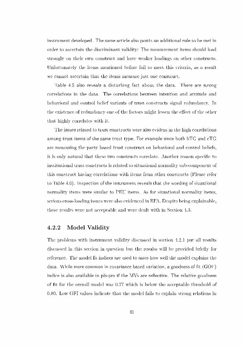
instrument developed. The same article also posits an additional rule to be met in

order to ascertain the discriminant validity: The measurement items should load

strongly on their own construct and have weaker loadings on other constructs.

Unfortunately the items mentioned before fail to meet this criteria, as a result

we cannot ascertain that the items measure just one construct.

Table 4.5 also reveals a disturbing fact about the data. There are strong

correlations in the data. The correlations between intention and attitude and

behavioral and control belief variants of trust constructs signal redundancy. In

the existence of redundancy one of the factors might lessen the e�ect of the other

that highly correlates with it.

The issues related to trust constructs were also evident in the high correlations

among trust items of the same trust type. For example since both bTG and cTG

are measuring the party based trust construct on behavioral and control beliefs,

it is only natural that these two constructs correlate. Another reason speci�c to

institutional trust constructs is related to situational normality sub-component of

this construct having correlations with items from other constructs (Please refer

to Table 4.6). Inspection of the instrument reveals that the wording of situational

normality items were similar to PEU items. As for situational normality items,

serious cross-loading issues were also evidenced in EFA. Despite being explainable,

these results were not acceptable and were dealt with in Section 4.3.

4.2.2 Model Validity

The problems with instrument validity discussed in section 4.2.1 put all results

discussed in this section in question but the results will be provided brie�y for

reference. The model �t indices are used to asses how well the model explains the

data. While more common in covariance based variation, a goodness of �t (GOF)

indice is also available in pls-pm if the MVs are re�ective. The relative goodness

of �t for the overall model was 0.77 which is below the acceptable threshold of

0.80. Low GFI values indicate that the model fails to explain strong relations in

41

Table 4.6: Standardized Loadings of Manifest Variables on Latent Variables in

the Initial ModelcACC cSK cTI cTG cPEU bTI bTG bPEU bPU PBC SN ATT INT

cACC1 0.92 0.65 0.68 0.52 0.63 0.51 0.39 0.37 0.49 0.28 0.13 0.23 0.20

cACC2 0.96 0.73 0.67 0.56 0.69 0.49 0.41 0.35 0.51 0.38 0.31 0.34 0.32

cSK1 0.71 0.95 0.66 0.55 0.63 0.51 0.42 0.42 0.46 0.39 0.29 0.34 0.33

cSK2 0.67 0.91 0.65 0.58 0.6 0.56 0.53 0.5 0.53 0.3 0.2 0.25 0.26

cTI1 0.50 0.47 0.82 0.58 0.62 0.6 0.42 0.42 0.44 0.31 0.22 0.29 0.22

cTI2 0.48 0.54 0.82 0.61 0.50 0.72 0.47 0.42 0.46 0.27 0.15 0.29 0.25

cTI3 0.47 0.51 0.79 0.54 0.43 0.71 0.45 0.37 0.39 0.16 0.08 0.18 0.15

cTI4 0.66 0.61 0.76 0.41 0.57 0.51 0.35 0.35 0.52 0.29 0.19 0.19 0.2

cTI5 0.70 0.66 0.79 0.61 0.74 0.56 0.51 0.44 0.57 0.29 0.21 0.22 0.17

cTG1 0.50 0.53 0.54 0.84 0.63 0.52 0.68 0.55 0.53 0.23 0.13 0.15 0.15

cTG2 0.54 0.52 0.56 0.83 0.53 0.51 0.62 0.44 0.47 0.23 0.18 0.24 0.23

cTG3 0.45 0.49 0.59 0.86 0.54 0.52 0.62 0.51 0.45 0.26 0.18 0.27 0.27

cTG4 0.49 0.49 0.63 0.84 0.61 0.51 0.59 0.48 0.49 0.24 0.15 0.22 0.18

cTG5 0.47 0.52 0.60 0.86 0.57 0.54 0.61 0.56 0.46 0.25 0.17 0.19 0.17

cPEU1 0.64 0.62 0.61 0.63 0.85 0.45 0.50 0.48 0.48 0.33 0.21 0.26 0.2

cPEU2 0.61 0.52 0.66 0.58 0.89 0.50 0.52 0.61 0.58 0.36 0.19 0.25 0.19

cPEU3 0.61 0.61 0.68 0.60 0.90 0.52 0.50 0.55 0.61 0.37 0.19 0.27 0.23

bTI1 0.38 0.39 0.63 0.56 0.47 0.84 0.68 0.65 0.56 0.15 0.13 0.27 0.21

bTI2 0.33 0.37 0.60 0.50 0.43 0.87 0.68 0.60 0.58 0.14 0.1 0.27 0.24

bTI3 0.40 0.44 0.62 0.48 0.45 0.81 0.56 0.40 0.44 0.13 0.13 0.26 0.2

bTI4 0.60 0.60 0.66 0.44 0.45 0.75 0.52 0.51 0.60 0.21 0.16 0.22 0.2

bTI5 0.50 0.57 0.57 0.50 0.42 0.73 0.61 0.65 0.55 0.17 0.19 0.16 0.21

bTG1 0.35 0.44 0.46 0.59 0.45 0.65 0.85 0.59 0.60 0.11 0.07 0.14 0.12

bTG2 0.35 0.38 0.45 0.61 0.48 0.58 0.85 0.59 0.58 0.23 0.19 0.22 0.13

bTG3 0.44 0.47 0.52 0.68 0.50 0.70 0.89 0.65 0.53 0.13 0.18 0.26 0.23

bTG4 0.31 0.43 0.44 0.63 0.53 0.69 0.85 0.69 0.53 0.12 0.14 0.18 0.16

bPEU1 0.31 0.48 0.47 0.54 0.55 0.63 0.66 0.91 0.59 0.24 0.18 0.21 0.21

bPEU2 0.39 0.44 0.47 0.57 0.60 0.66 0.69 0.95 0.66 0.27 0.20 0.29 0.24

bPU1 0.53 0.51 0.56 0.52 0.52 0.66 0.60 0.68 0.90 0.32 0.22 0.36 0.37

bPU2 0.44 0.46 0.54 0.51 0.63 0.57 0.57 0.56 0.92 0.36 0.28 0.39 0.33

PBC1 0.31 0.36 0.29 0.21 0.33 0.16 0.11 0.23 0.29 0.88 0.54 0.65 0.53

PBC2 0.25 0.25 0.25 0.20 0.30 0.14 0.13 0.21 0.30 0.82 0.52 0.61 0.54

PBC3 0.31 0.34 0.29 0.23 0.33 0.14 0.10 0.18 0.34 0.86 0.58 0.71 0.61

PBC4 0.35 0.33 0.34 0.33 0.40 0.22 0.25 0.33 0.35 0.86 0.51 0.57 0.53

SN1 0.18 0.22 0.21 0.19 0.17 0.18 0.19 0.24 0.21 0.51 0.80 0.64 0.61

SN2 0.19 0.19 0.20 0.11 0.16 0.16 0.17 0.14 0.20 0.49 0.79 0.67 0.58

SN3 0.27 0.26 0.16 0.22 0.23 0.11 0.14 0.14 0.24 0.46 0.77 0.53 0.58

SN4 0.16 0.18 0.14 0.09 0.16 0.09 0.07 0.12 0.23 0.55 0.83 0.59 0.58

ATT1 0.25 0.25 0.24 0.22 0.20 0.22 0.18 0.19 0.34 0.70 0.68 0.91 0.74

ATT2 0.33 0.32 0.27 0.24 0.30 0.27 0.21 0.26 0.40 0.71 0.70 0.94 0.78

ATT3 0.22 0.21 0.26 0.17 0.21 0.26 0.19 0.22 0.34 0.62 0.65 0.88 0.70

ATT4 0.32 0.34 0.30 0.27 0.32 0.32 0.27 0.30 0.39 0.62 0.68 0.85 0.80

INT1 0.22 0.26 0.14 0.19 0.18 0.16 0.14 0.14 0.32 0.52 0.66 0.73 0.90

INT2 0.27 0.28 0.19 0.16 0.13 0.22 0.14 0.23 0.29 0.52 0.61 0.67 0.83

INT3 0.28 0.31 0.25 0.22 0.25 0.24 0.17 0.22 0.33 0.60 0.65 0.78 0.92

INT4 0.24 0.29 0.29 0.26 0.25 0.29 0.23 0.25 0.41 0.62 0.66 0.80 0.86

42

the data. The model must be modi�ed in order to increase the model �t.

[43] posited that the GOF indices alone were not representative of the model's

validity alone and that the model's predictive power (R2) and explanatory power

(path coe�cients) should also be discussed to evaluate a models validity.

The R2 value for this initial model was 0.74 but this �nding su�ered from

instrumental validity issues and could not be deemed conclusive.

Figure 4.3 shows the path coe�cients among latent variables and standardized

loadings of MVs on LVs. As can be seen, the measurement model �ts perfectly

whereas path coe�cients for some LVs in the structural model are too low to be

deemed meaningful. Especially the trust constructs have low e�ects contrary to

the expectations. It has been inferred that the problems with the path coe�cients

might be due to the e�ect of various constructs overloading each other out due

to multicollinearity and redundancy. These problems have been dealt with in

Section 4.3.

43

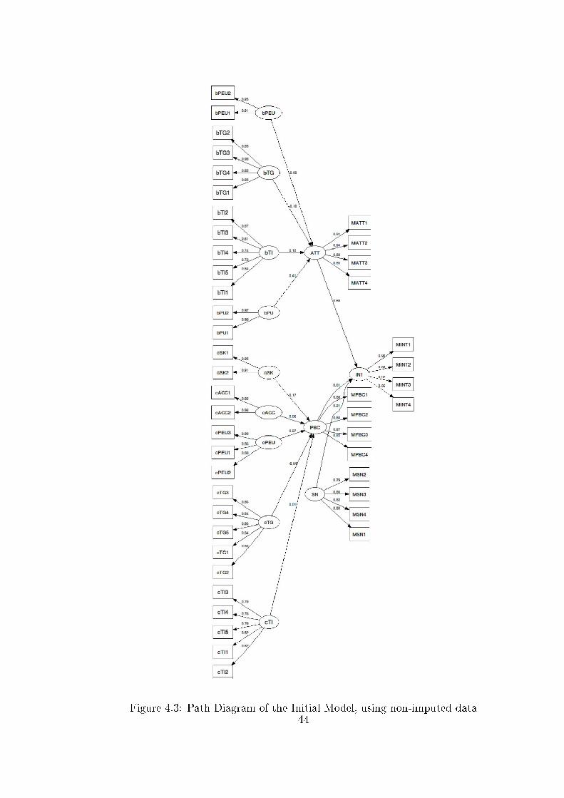
Figure 4.3: Path Diagram of the Initial Model, using non-imputed data44

4.3 Model Modi�cation

The initial model tested in Section 4.2 su�ered from instrument and model va-

lidity issues and was un�t for use in a scienti�c study. The standard procedure

in SEM studies involve formulating a model based on theory and modifying this

model based on modi�cation indices and other indicators of relations in data [32].

The key to model modi�cation is not to loose the theoretical support of the model

by following the �t indices blindly, disregarding the previous theory. The initial

model was modi�ed iteratively, making one change at a time and observing the

e�ect of changes in the model �t, R2, bootstrap t-test results and path loadings.

Each iteration was backed with proper reasoning based on theory or logical rea-

soning. This approach was similar to the ones suggested in [38, 30]. After 16

iterations the following changes were applied to the �nal model. Figure 4.4 shows

the path diagram of this �nal modi�ed model.

4.3.1 Measurement Model

The �rst step of modi�cation in this study was the modi�cation of the measure-

ment model to minimize unwanted correlations among LVs. This was achieved

by removing or combining problematic items in the measurement model.

The EFA results in Table 4.1 and EVA values in Table 4.5 indicated that the

measures for subjective norms construct were problematic. The removal of the

problematic items left subjective norms construct with a single manifest variable

and even then the goodness of �t index was sub-par, thus the complete removal

of subjective norms construct was decided. The same results also pointed that

the fourth item of attitude construct did not load as expected on the attitude

construct, thus this item was removed from the measurement model.

The EFA results in Table 4.2, Table 4.3 and EVA values in Table 4.5 indicated

that situational normality sub-component of institutional trust construct loaded

stronger with other items. The removal of the fourth and the �fth manifest

variables improved the AVE value of institutional trust considerably.

45

Another modi�cation to the measurement model was the integration of skills

and access constructs into the higher order local factors construct. As is evident

in the EFA in Table 4.3 these two items loaded strongly together. Both skills and

access constructs measure the perceptions of people towards the use of computers.

Since computer skills and access to computers is a factor of the socio-cultural

strata and the position in digital divide, this common factor was named local

factors.

4.3.2 Structural Model

After the modi�cations to the measurement model, there were modi�cations to

be made to the structural model.

The �rst modi�cation was linking perceived usefulness and perceived ease of

use constructs of behavioral beliefs. This modi�cation was made in accordance

with suggestions on the previous literature on TAM which stated that perceived

ease of use was often mediated through perceived usefulness [33, 1].

The second modi�cation was to gather all trust constructs under a single trust

construct and linking this trust construct to other endogenous latent variables in

order to test the theoretical connections listed in the Section 3.1. Table 4.5 shows

that the trust constructs had high correlations among themselves. Some amount

of correlation can be due to the shared latent variable (Trust) which was not

included in the initial model. Also there were two variants (one for behavioral

and one for control beliefs) for both party based and institutional trust in line

with the suggestions of Ajzen [24]. Not mediating the e�ects of di�erent trust

types by a common latent variable (Trust) caused the trust types to overload

each others' e�ects. By including two variants in separate latent variables this

was taken even further by mediating the e�ects in higher order LVs. The new

relation between intention and trust had been used in a variety of e-government

adoption studies (See Section 2.1.2). The other relations did not require any

changes to the theoretical justi�cations provided in Section 3.1.

46

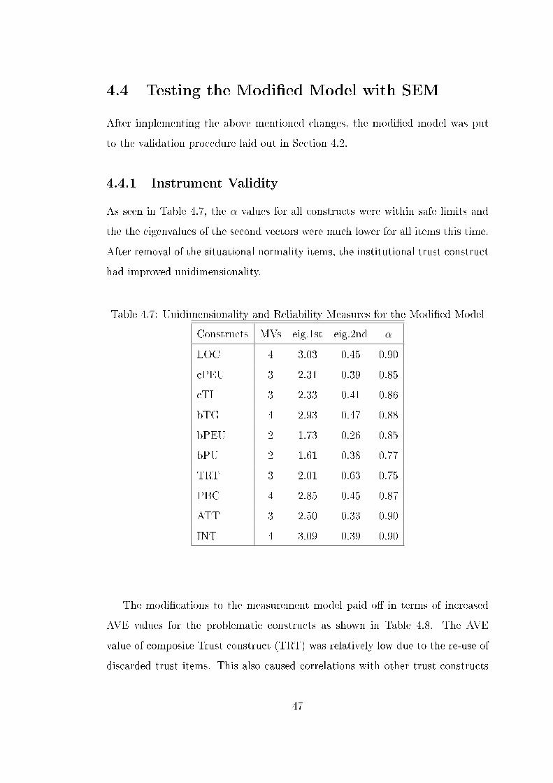
4.4 Testing the Modi�ed Model with SEM

After implementing the above mentioned changes, the modi�ed model was put

to the validation procedure laid out in Section 4.2.

4.4.1 Instrument Validity

As seen in Table 4.7, the α values for all constructs were within safe limits and

the the eigenvalues of the second vectors were much lower for all items this time.

After removal of the situational normality items, the institutional trust construct

had improved unidimensionality.

Table 4.7: Unidimensionality and Reliability Measures for the Modi�ed Model

Constructs MVs eig.1st eig.2nd α

LOC 4 3.03 0.45 0.90

cPEU 3 2.31 0.39 0.85

cTI 3 2.33 0.41 0.86

bTG 4 2.93 0.47 0.88

bPEU 2 1.73 0.26 0.85

bPU 2 1.61 0.38 0.77

TRT 3 2.01 0.63 0.75

PBC 4 2.85 0.45 0.87

ATT 3 2.50 0.33 0.90

INT 4 3.09 0.39 0.90

The modi�cations to the measurement model paid o� in terms of increased

AVE values for the problematic constructs as shown in Table 4.8. The AVE

value of composite Trust construct (TRT) was relatively low due to the re-use of

discarded trust items. This also caused correlations with other trust constructs

47

but none of the values were alarming. Square roots of AVE values were much

higher than the correlations to other items for all items indicating convergent and

discriminant validity.

Table 4.8: Correlations Among Latent Variables and AVE Values for the Modi�ed

Model

LVs LOC cPEU cTI bTG bPEU bPU TRT PBC ATT INT

LOC 1.00 0.73 0.62 0.53 0.49 0.64 0.58 0.45 0.39 0.38

cPEU 0.74 1.00 0.62 0.58 0.67 0.68 0.62 0.50 0.35 0.31

cTI 0.62 0.61 1.00 0.53 0.48 0.51 0.78 0.35 0.35 0.30

bTG 0.53 0.58 0.53 1.00 0.67 0.64 0.76 0.22 0.28 0.29

bPEU 0.49 0.67 0.49 0.67 1.00 0.67 0.63 0.35 0.30 0.28

bPU 0.64 0.68 0.51 0.64 0.67 1.00 0.63 0.44 0.45 0.42

TRT 0.58 0.62 0.77 0.76 0.63 0.62 1.00 0.28 0.37 0.36

PBC 0.44 0.50 0.35 0.22 0.34 0.44 0.28 1.00 0.71 0.61

ATT 0.39 0.35 0.35 0.28 0.30 0.45 0.37 0.70 1.00 0.77

INT 0.38 0.32 0.30 0.29 0.27 0.42 0.36 0.60 0.77 1.00

AVE 0.76 0.77 0.78 0.74 0.87 0.81 0.67 0.71 0.84 0.78√

AV E 0.87 0.88 0.88 0.86 0.93 0.91 0.82 0.84 0.92 0.88

Table 4.9 shows the item loadings on latent variables. As previously dis-

cussed in Section 4.2 high loadings on corresponding construct are indicators of

convergent validity whereas low loadings on other constructs are indicators of

discriminant validity. As seen in Table 4.9 all items met this criteria.

Table 4.10 shows the bootstrap t-test results for loadings of MV on their

respective LV. The bootstraping procedure re-samples the data 200 times with a

sample size of 100 and runs the analysis on each sample. This allows to observe

various possible subsamples that could have come up in the population from the

data at hand. Then the mean values of boot samples are compared to the original

sample to see if there is a statistically signi�cant di�erence. P value indicates how

48

Table 4.9: Standardized Loadings of Manifest Variables on Latent Variables in

the Modi�ed Model

LOC cPEU TI TG bPEU bPU TRT PBC ATT INT

cSK1 0.89 0.64 0.55 0.44 0.45 0.55 0.52 0.44 0.38 0.39

cSK2 0.84 0.62 0.55 0.57 0.54 0.60 0.55 0.33 0.29 0.30

cACC1 0.87 0.62 0.55 0.43 0.39 0.56 0.48 0.34 0.31 0.28

cACC2 0.90 0.69 0.54 0.44 0.37 0.56 0.49 0.44 0.37 0.36

cPEU1 0.64 0.85 0.53 0.45 0.53 0.50 0.50 0.43 0.30 0.25

cPEU2 0.63 0.89 0.54 0.54 0.65 0.63 0.59 0.44 0.30 0.27

cPEU3 0.67 0.89 0.56 0.52 0.59 0.65 0.54 0.45 0.34 0.32

cTI1 0.54 0.62 0.84 0.45 0.43 0.46 0.64 0.36 0.34 0.29

cTI2 0.57 0.56 0.90 0.48 0.47 0.48 0.73 0.34 0.34 0.28

cTI3 0.54 0.46 0.91 0.47 0.39 0.41 0.69 0.23 0.25 0.22

bTG1 0.46 0.49 0.46 0.87 0.58 0.61 0.64 0.18 0.21 0.20

bTG2 0.45 0.51 0.42 0.85 0.54 0.61 0.58 0.27 0.29 0.23

bTG3 0.46 0.47 0.47 0.85 0.55 0.47 0.70 0.14 0.23 0.29

bTG4 0.45 0.50 0.44 0.86 0.62 0.52 0.67 0.17 0.24 0.26

bPEU1 0.46 0.61 0.44 0.61 0.93 0.61 0.56 0.30 0.24 0.25

bPEU2 0.46 0.65 0.47 0.64 0.94 0.64 0.61 0.34 0.31 0.27

bPU1 0.60 0.54 0.47 0.61 0.60 0.90 0.55 0.36 0.41 0.44

bPU2 0.56 0.68 0.45 0.55 0.61 0.90 0.58 0.42 0.41 0.32

bTI2 0.42 0.46 0.65 0.66 0.59 0.56 0.83 0.19 0.32 0.27

bTI3 0.51 0.49 0.67 0.62 0.44 0.51 0.86 0.18 0.29 0.27

cTG3 0.50 0.58 0.59 0.59 0.52 0.46 0.76 0.31 0.28 0.34

PBC1 0.43 0.41 0.30 0.19 0.27 0.36 0.23 0.88 0.63 0.52

PBC2 0.33 0.40 0.25 0.18 0.29 0.36 0.24 0.82 0.55 0.48

PBC3 0.40 0.43 0.33 0.15 0.28 0.40 0.22 0.86 0.69 0.57

PBC4 0.35 0.44 0.29 0.23 0.33 0.37 0.24 0.83 0.50 0.47

ATT1 0.26 0.26 0.26 0.20 0.21 0.33 0.27 0.65 0.87 0.69

ATT2 0.43 0.38 0.34 0.29 0.32 0.47 0.37 0.68 0.95 0.75

ATT3 0.36 0.31 0.35 0.27 0.28 0.43 0.35 0.61 0.92 0.68

INT1 0.31 0.25 0.19 0.21 0.19 0.35 0.29 0.48 0.66 0.90

INT2 0.35 0.21 0.22 0.21 0.26 0.33 0.25 0.50 0.62 0.84

INT3 0.35 0.33 0.30 0.27 0.26 0.37 0.34 0.56 0.70 0.92

INT4 0.35 0.32 0.32 0.30 0.26 0.42 0.36 0.58 0.73 0.86

49

likely it is to observe the original data in comparison to the bootstrapped samples.

A p value lower than 5% would have indicated that the observation in the original

sample was due to change. The results reveal that the loading values were not

statistically di�erent between bootstrapped and original data at a 0.95 con�dence

interval except for the attitude item 2 and the intention item 3. Even those values

are reasonably close to the limit.

50

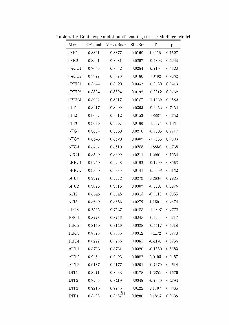
Table 4.10: Bootstrap validation of Loadings in the Modi�ed Model

MVs Original Mean.Boot Std.Err T p

cSK1 0.8861 0.8877 0.0160 1.4115 0.1597

cSK2 0.8391 0.8381 0.0297 -0.4898 0.6248

cACC1 0.8656 0.8642 0.0284 -0.7194 0.4728

cACC2 0.8977 0.8978 0.0180 0.0462 0.9632

cPEU1 0.8544 0.8520 0.0357 -0.9539 0.3413

cPEU2 0.8894 0.8894 0.0192 -0.0312 0.9752

cPEU3 0.8932 0.8917 0.0187 -1.1339 0.2582

cTI1 0.8417 0.8409 0.0363 -0.3252 0.7454

cTI2 0.9002 0.9012 0.0153 0.8887 0.3752

cTI3 0.9086 0.9067 0.0166 -1.6374 0.1031

bTG1 0.8664 0.8660 0.0210 -0.2905 0.7717

bTG2 0.8546 0.8520 0.0302 -1.2033 0.2303

bTG3 0.8492 0.8510 0.0288 0.8858 0.3768

bTG4 0.8590 0.8609 0.0211 1.2991 0.1954

bPEU1 0.9250 0.9248 0.0192 -0.1299 0.8968

bPEU2 0.9390 0.9385 0.0141 -0.5063 0.6132

bPU1 0.8977 0.8982 0.0279 0.2634 0.7925

bPU2 0.9023 0.9015 0.0307 -0.3891 0.6976

bTI2 0.8348 0.8346 0.0315 -0.0811 0.9355

bTI3 0.8640 0.8663 0.0279 1.1601 0.2474

cTG3 0.7565 0.7527 0.0488 -1.0897 0.2772

PBC1 0.8773 0.8766 0.0248 -0.4244 0.6717

PBC2 0.8159 0.8146 0.0328 -0.5517 0.5818

PBC3 0.8576 0.8585 0.0312 0.4172 0.6770

PBC4 0.8297 0.8286 0.0365 -0.4191 0.6756

ATT1 0.8735 0.8731 0.0320 -0.1660 0.8683

ATT2 0.9484 0.9496 0.0082 2.0105 0.0457

ATT3 0.9187 0.9177 0.0201 -0.7379 0.4614

INT1 0.8971 0.8988 0.0178 1.3851 0.1676

INT2 0.8436 0.8419 0.0348 -0.7086 0.4794

INT3 0.9216 0.9235 0.0122 2.1797 0.0305

INT4 0.8583 0.8587 0.0280 0.1845 0.853851

4.4.2 Model Validity

The modi�cations to the initial model paid o� in terms of goodness of �t indice

(GFI) values. Please refer to Table 4.11 to see comparative results of various

measures of GFI. The relative GFI for this modi�ed model is 0.85, above the

acceptable threshold of 0.80. This indicates that the proposed model explains a

considerable amount of relations in data. The GFI for the structural model has

also improved signi�cantly in this modi�ed model.

Table 4.11: Comparative Goodness of Fit Results

GFI Initial Model Modi�ed Model

Absolute 0.53 0.59

Relative 0.77 0.85

Measurement 0.997 0.999

Structural 0.60 0.72

The R2 value represents the predictive power of the model and the model

was successful in predicting the intentions. Table 4.12 lists R2 values for all

endogenous latent variables. The R2 value of intention for this new model was

0.61. Though seemingly lower than the initial model this result was free of the

problems regarding instrumental validity and was conclusive. The �nal model

explains 61% of the variation in the data.

The path coe�cients can be seen in both Table 4.13 and Figure 4.4. Path

coe�cients are similar to regression coe�cients in regression analysis; they rep-

resent the e�ect of a latent variable on the target latent variable. In our model

for example, a one point change in attitudes would cause 0.67 points change in

intentions. Table 4.13 shows the bootstrap validation of path coe�cients. Ac-

cording to the results of bootstrap validation, all paths were valid and �t for

interpretation.

52

Table 4.12: R2 Values for Endogenous Latent Variables.

LV R2

INTENTION 0.61

ATTITUDE 0.22

PBC 0.26

TRUST 0.78

PU 0.45

Table 4.13: Bootstrap validation of Path Coe�cients in The Structural Model

PATH Original Mean.Boot Std.Err t.statis p.value

ATT → INT 0.6655 0.6638 0.0951 -0.2521 0.8012

PBC → INT 0.1122 0.1115 0.0781 -0.1314 0.8956

TRT → INT 0.0813 0.0883 0.0566 1.7409 0.0832

TRT → ATT 0.1612 0.1608 0.0887 -0.0576 0.9542

bPU → ATT 0.4018 0.3993 0.1055 -0.3344 0.7384

bPEU → ATT -0.0733 -0.0681 0.0855 0.8612 0.3902

bPEU → bPU 0.6721 0.6723 0.0528 0.0549 0.9563

TG → TRT 0.4875 0.4930 0.0431 1.8212 0.0701

TI → TRT 0.5207 0.5164 0.0419 -1.4535 0.1477

cPEU → PBC 0.3650 0.3671 0.0780 0.3833 0.7019

cLOC → PBC 0.1806 0.1880 0.0733 1.4220 0.1566

53

4.4.3 Model Interpretation

Figure 4.4 shows the path diagram of the modi�ed model. The factor loadings

of all manifest variables were strong, indicating a strong measurement model.

When interpreting either factor loadings or path coe�cients two factors should

be considered: (1) Is the loading/path statistically valid? (2) Is the loading/path

strong? Bootstrap tests revealed that the factor loadings were statistically sig-

ni�cant. The loadings of all manifest variables were strong (>0.80), indicating a

strong measurement model.

The bootstrap tests for path coe�cients show that the path coe�cients were

also reliable. It is argued that the path coe�cients should be at least 0.10 to

account for a considerable amount of variance in the latent variable they relate

to. Table 4.14 shows the e�ect of mediated relations through the indirect e�ects,

direct e�ects and total e�ects. The indirect e�ect size is a factor of all path

coe�cients between two LVs which are at least two edges apart. The total e�ects

in the table are composed of both direct and mediated relationships among LVs.

It can be seen in this table that the paths with small direct e�ect sizes (<.10)

had considerable total e�ect sizes in the end.

The attitudes had the strongest e�ect on the intentions as expected. The

attitudes was followed by PBC with the second largest direct e�ect on intentions.

As expected, the salient beliefs had the proposed relations with predictor vari-

ables. PU was very in�uential in predicting attitudes. Trust was the second most

in�uential �gure in predicting attitudes. TI and TG together explained almost

equal amount of variance in trust and explained 70% of it. PEU and LOC played

signi�cant roles in predicting PBC.

Interpretation of path coe�cients revealed two �ndings that deviated slightly

from the expectations.

Trust seemingly had a minuscule direct e�ect with a path coe�cient of 0.08

on intentions. The e�ect of trust on attitudes was 0.16. When the e�ect of trust

on intention mediated by attitudes were considered, the total e�ect size for trust

54

Figure 4.4: Path Diagram of the Modi�ed Model, using non imputed data

55

Table 4.14: E�ect Sizes in the Modi�ed Model

Relationship Dir. E�ects Ind. E�ects Tot. E�ects

ATT → INT 0.67 0.00 0.67

PBC → INT 0.11 0.00 0.11

TRT → INT 0.08 0.11 0.19

TRT → ATT 0.16 0.00 0.16

bPU → ATT 0.40 0.00 0.40

bPU → INT 0.00 0.27 0.27

bPEU → bPU 0.67 0.00 0.67

bPEU → ATT -0.07 0.27 0.20

bPEU → INT 0.00 0.13 0.13

TI → TRT 0.52 0.00 0.52

TI → ATT 0.00 0.08 0.08

TI → INT 0.00 0.10 0.10

TG → TRT 0.49 0.00 0.49

TG → ATT 0.00 0.08 0.08

TG → INT 0.00 0.09 0.09

cPEU → PBC 0.37 0.00 0.37

cPEU → INT 0.00 0.04 0.04

cLOC → PBC 0.18 0.00 0.18

cLOC → INT 0.00 0.02 0.02

56

on intention was 0.19. When included in the model, the relationship between

Trust and PBC hypothesized in the initial model reduced the model �t without

increasing the amount of variance explained. The bootstrap validation of the path

between PBC and TRUST also failed, indicating an insigni�cant path. Thus the

proposed path was removed from the �nal model.

The relation between perceived ease of use and attitude did not show up as

expected in the model. Yet, the previous research has shown that perceived

usefulness can be mediated over perceived usefulness [1, 33]. That was also the

case in our model and was evident in strong path coe�cients between PEU and

PU in the model.

The rest of the relations were proved to be as assumed in the model.

4.4.4 Comparison to Alternate Models

Apart from the 16 alternate models tested in the model modi�cation section

(Please refer to Section 4.3), the �nal model was compared to the legendary

Technology Acceptance Model [1]. Figure 4.5 shows the structural model for

TAM. Manifest variables were not included to simplify the �gure. All loadings of

MVs were higher than 0.80.

Figure 4.5: Alternate Model: TAM

57

The TAM model had a relative GFI value of 0.86, a seemingly 0.01 point

increase over the �nal model. It should be kept in mind however, that the data

set used for TAM model was much smaller. The TAM model consists of only

three latent variables with eight manifest variables in comparison to the ten latent

variables and thirty-two manifest variables of the �nal model. Meaning it has less

variance to account for.

All paths in both models were valid but TAM model also su�ered from neg-

ative loadings of PEU due to mediation through PU. The total e�ect of PU on

intentions was 0.41 and PEU on intentions was 0.24.

The Achilles' heel for the TAM model was predictive power as was pointed

in [13]. The R2 value of intention for TAM was 0.15 a signi�cant reduction in

comparison to 0.61 provided by the �nal model. This result proves that the �nal

model was far superior in comparison to TAM.

4.5 Reconsidering The Proposed Hypothesis

After the changes to the model in Section 4.3, the �t of both the measurement

model and the structural model improved. Both the instrument and the model

had been validated in Section 4.4. The �nal model required the changes to the

proposed relations discussed in Section 3.1, those changes are discussed below.

The modi�ed model and the new hypotheses can be seen in Figure 4.6.

By removing SN construct, the chance to prove or disprove the H4 was lost,

and this relation was removed.

H6a was proven but the e�ect of PEU on attitudes was completely mediated

by PU. The relation between PU and PEU had to be formulated as H6c.

H6c PEU will have a positive e�ect on the PU of the e-government service.

With the inclusion of a higher order trust latent variable the hypothesized

relations H7a, H7b and H8a, H8b were changed. These relations had to be

58

re-formulated to re�ect the relations mediated over the trust construct. Unfor-

tunately the path between trust and PBC could not be validated in bootstraps

so the relationship between trust and PBC could not be validated and H7b and

H8b were removed. The role of trust on attitudes formulated in H7a and H8a

were combined under H7. Other than the partially mediated e�ect of trust over

attitudes, the analysis brought forth the existence of a direct relation between

trust and intention which was not initially theorized. This relation had previously

been proven in many e-government adoption models (See Section 2.1.2), and was

now formulated as H11. The relations between TG and TI and trust had been

formulated as H12 and H13.

H7 Trust will have a positive e�ect on the attitude toward the use of e-government

service.

H11 Trust will have a positive e�ect on the intention to use the e-government

service.

H12 TI will have a positive e�ect on trust.

H13 TG will have a positive e�ect on the trust.

The skills and access were combined under the local factors construct. Thus

the H9 and H10 had to be combined under H14. The IT penetration will have a

positive e�ect on perceived behavioral control [11].

H14 Local factors will have a positive e�ect on the PBC to use the e-government

service.

The rest of the hypothesized relations were proven. Table 4.15 shows the

hypothesis number in the initial model, the number in the �nal model and the

�nal status of the hypothesis after PLS-PM validation. The �nal model, although

di�erent from the initially proposed model, was more like a re�ned and rephrased

version of the initial model since it did not require a major overhaul of the un-

derlying theoretical basis.

59

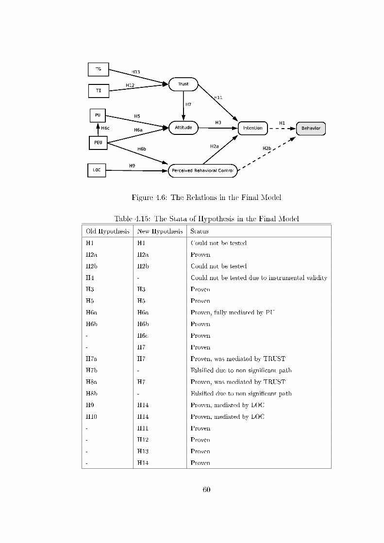
Figure 4.6: The Relations in the Final Model

Table 4.15: The Stata of Hypothesis in the Final Model

Old Hypothesis New Hypothesis Status

H1 H1 Could not be tested

H2a H2a Proven

H2b H2b Could not be tested

H4 - Could not be tested due to instrumental validity

H3 H3 Proven

H5 H5 Proven

H6a H6a Proven, fully mediated by PU

H6b H6b Proven

- H6c Proven

- H7 Proven

H7a H7 Proven, was mediated by TRUST

H7b - Falsi�ed due to non signi�cant path

H8a H7 Proven, was mediated by TRUST

H8b - Falsi�ed due to non signi�cant path

H9 H14 Proven, mediated by LOC

H10 H14 Proven, mediated by LOC

- H11 Proven

- H12 Proven

- H13 Proven

- H14 Proven

60

CHAPTER 5

CONCLUSION

This chapter discusses the �ndings of , lists the limitations to and proposes venues

for further research for this study.

5.1 Summary of the Study

As the e-government initiatives gain traction, the need to better understand this

phenomena is gaining importance. The models for adoption of G2C e-government

services have the potential to provide the much needed insight into the adoption

behavior. To this end, this study has developed and validated an e-government

adoption model based on the theory of planned behavior (TPB). TPB has served

for years in diverse domains to predict and explain human behavior. With this

study, TPB was employed in e-government context and validated by contempo-

rary statistical techniques.

The Partial Least Squares Path Modelling (PLS-PM), a variation of Structural

Equation Modelling (SEM), was employed in this study to validate both the

measurement instrument and the proposed model. The initial model had to be

modi�ed to increase the model �t, explanatory power and the instrument validity,

but these modi�cations are also a part of standard SEM conduct. Although the

�nal model at hand was not the initially proposed model, the �nal model was

61

more like a re�ned, rephrased version of the initial model. Most of the proposed

relationships in the model was preserved and the others were altered without any

change to the underlying theoretical foundations.

The study investigated and uncovered the factors e�ecting the intention to

use the KYK electronic services. The results of the PLS-PM analysis proved, as

is evidenced by high R2 value (Please refer to Table 4.12) of intentions in the �nal

model, that the predictor variables of the theory of planned behavior actually do

predict the e-government adoption behavior well.

Path coe�cients in the model reveal that attitudes got the lion's share in

explaining the intentions. This is in-line with the expectations and the previous

literature [4]. The Perceived Behavioral Control (PBC) had the second largest

direct e�ect on intentions in our model, based on the data at hand. This shows

that the PBC actually plays a role in the forming the intentions to use the KYK

services. While PBC had the second largest direct e�ect, it was shadowed by the

total e�ect of combined trust.

The role of trust was partially mediated over attitudes. This means that

trust both precedes the attitudes and the intentions. The e�ect of trust on the

intentions is composed of both a direct e�ect and an indirect e�ect over the

attitudes. In our model Trust was the second most in�uential construct due

to the large total e�ect size (See Table 4.14), proving the importance of trust

in e-government setting. This importance was also emphasized in a number of

previous studies [16, 11, 20, 21, 23]. The role of Trust on PBC however could not

be proven due to non-signi�cant path loading. It should be kept in mind however,

it is not recommended to generalize the PLS results to the general population and

this might be due to a sample speci�c issue. The role of Trust on PBC should

be investigated with a multivariate normal data set in covariance based SEM if

conclusive results are desired.

The Perceived Usefulness (PU) proved to be a strong determinant of attitudes

as expected. The Perceived Ease of Use (PEU) on the other hand was totally

mediated by PU, and had no direct e�ect of its own in the presence of PU. This

62

was expected as the previous studies have con�rmed such a structure [1].

Trust in internet and trust in government seemingly explain almost all of the

variance in combined trust construct. How ever, this �nding should be taken

with a pinch of salt. Since the initial model did not poses a combined trust

construct and PLS method we employed required Manifest Variables (MV) for

every Latent Variables (LV) to be estimated. Hence we integrated three of the

surplus items that originated from the discarding of extra trust belief types in

forming the combined trust LV. For a more accurate estimation of the variance

explained by TI and TG in combined trust construct the use of items from a

unitary trust scale �which we lacked� would have been better.

The �ndings of the model also proved the relations between PBC and PEU

and PBC and local factors for our sample.

5.2 Limitations

Implementing TPB, a theory more than two decades old, strictly as suggested

by Ajzen [14, 4, 12, 24] created some complications uncovered with the modern

analytical techniques as was evidenced in the Chapter 4. First of all, employ-

ing separate belief constructs for behavioral and control belief types of the same

salient belief (such as trust in internet in our study) created a shared correlation

among the constructs which caused multicollinearity. This would cause the con-

structs to reduce each others' e�ects, messing the path coe�cients. Furthermore

if left out of the model this relation would reduce the overall model �t. For future

reference; in SEM techniques using multi method approach is clearly the superior

method, if not, a single construct for a single salient belief is clearly a better

choice than integrating two versions of the same method.

Another complication was caused by formating the items in the measurement

model in line with Ajzen's guidelines [12]. Ajzen suggested de�ning each item in

the questionnaire in terms of TACT and the wording of items were further de�ned

according to salient belief types. This similarity of the items in the questionnaire

63

caused a method halo �a disturbance in the data caused by the instrument. This

created correlations due to the sentence structure among similarly worded items

and further multicollinearity. It is now clear that de�ning all items in such similar

manner blurs the �ndings in SEM analysis. It would be wise to mention TACT in

the instructions section of each set of questions and reduce the length of questions

in future work.

Investigating the role of Subjective Norms (SN) would have made the �nal

model a complete TPB study. Unfortunately however, the items derived from

[24] for the SN construct failed the factorial validity tests, thus the e�ect of

subjective norms could not be observed. The items for SN should have been

de�ned in narrower terms for better instrument validity. This should be taken

into account in any follow-up studies.

This study was conducted on a particular e-government service from KYK

with a very special sample � young people with high computer access � and in

order for the results to be generalizable the �ndings should be proven in other

studies.

5.3 Implication for Future Research

One venue for future research would be to test the model in an inter-cultural

setting. According to 2005 OECD �gures the number of Internet users is one

�fth of the European average in Turkey [5]. Comparing a developed country with

Turkey might better uncover the role of IT penetration in e-government adoption.

Another possible route for future research would be to improve the explana-

tory power of the model further. Since the TPB implemented in this study

stayed �rmly true to Ajzen's guidelines except for the elicitation of salient be-

liefs. Instead of eliciting salient beliefs a�ecting the adoption behavior from the

population, this study used the salient beliefs derived from the literature. The

derived constructs of perceived usefulness, perceived ease of use, local factors,

trust in government and trust in Internet contributed to the explanatory power

64

of the model. Although the R2 value for intentions and trust were beyond sat-

isfactory, the R2 values for attitudes and PBC were sub-par (see. Table 4.12.

This indicates that there is room for improvement in explaining and predicting

attitudes and PBC. To enhance the explanatory power of the model the factors

in�uencing these constructs should be investigated, either by elicitation of salient

beliefs or by more constructs derived from the literature. Further research into

uncovering these factors would be a worthwhile e�ort, increasing the explanatory

power and the usefulness of the model.

65

REFERENCES

[1] F. D. Davis, �Perceived usefulness , perceived ease of use , and user accep-

tance of information technology,� MIS Quarterly, vol. 13, no. 3, pp. 319�339,

September 1989.

[2] G. C. Moore and I. Benbasat, �Development of an instrument to measure the

perceptions of adopting an information technology innovation,� Information

Systems Research, vol. 2, pp. 192�222, 1991.

[3] V. Venkatesh, M. G. Morris, G. B. Davis, and F. D. Davis, �User acceptance

of information technology: Toward a uni�ed view,� MIS Quarterly, vol. 27,

no. 3, pp. 425�478, September 2003.

[4] I. Ajzen, �The theory of planned behavior,� Organizational Behavior and

Human Decision Processes, vol. 50, pp. 179�211, 1991.

[5] Organization for Economic Cooperation & Development, Oecd E-

Government Studies: Turkey (OECD E-Government Studies). Organization

for Economic Cooperation & Devel, February 2004.

[6] United Nations Department of Economic and Social A�airs, �Un e-

government survey 2008: From e-government to connected governance,�

United Nations, Tech. Rep., 2008.

[7] M. Claps, �Western europe, government sector, it spending forecast,

2004�2009,� IDC, Tech. Rep., 2005.

66

[8] R. Heeks, �egovernment for development information exchange,� October

2008. [Online]. Available: http://www.egov4dev.org/success/sfrates.shtml

[9] D. H. McKnight, V. Choudhury, and C. Kacmar, �Developing and validating

trust measures for e-commerce: An integrative typology,� Info. Sys. Re-

search, vol. 13, no. 3, pp. 334�359, 2002.

[10] D. Gefen, E. Karahanna, and D. W. Straub, �Trust and tam in online shop-

ping: An integrated model,� MIS Quarterly, vol. 27, no. 1, pp. 51�90, March

2003.

[11] L. Carter and V. Weerakkody, �E-government adoption: A cultural compar-

ison,� Information Systems Frontiers, vol. 10, no. 4, pp. 473�482, 2008.

[12] I. Ajzen, �Perceived behavioral control , self-e�cacy , locus of control ,

and the theory of planned behavior,� Journal of Applied Social Psychology,

vol. 32, no. 4, pp. 665�683, 2002.

[13] I. Benbasat and H. Barki, �Quo Vadis , TAM?� Journal of the association

for information systems, vol. 8, no. 3, pp. 211�218, April 2007.

[14] I. Ajzen and M. Fishbein, �Attitudes and normative beliefs as factors in�u-

encing behavioral intentions,� Journal of Personality and Social Psychology,

vol. 21, pp. 1�9+, 1972.

[15] M. Bradford and J. Florin, �Examining the role of innovation di�usion fac-

tors on the implementation success of enterprise resource planning systems,�

International Journal of Accounting Information Systems, vol. 4, pp. 205�

225, 2003.

[16] L. Carter and F. Bélanger, �The utilization of e-government services:

citizen trust , innovation and acceptance factors,� Information Sys-

tems Journal, vol. 15, no. 1, pp. 5�25, 2005. [Online]. Available:

http://dx.doi.org/10.1111/j.1365-2575.2005.00183.x

67

[17] W. A. Conklin, �Barriers to adoption of e-government,� in HICSS '07: Pro-

ceedings of the 40th Annual Hawaii International Conference on System Sci-

ences. Washington , DC , USA: IEEE Computer Society, 2007, p. 98.

[18] P. A. Pavlou, �Consumer acceptance of electronic commerce: Integrating

trust and risk with the technology acceptance model,� Int. J. Electron. Com-

merce, vol. 7, no. 3, pp. 101�134, 2003.

[19] P. A. Pavlou and M. Fygenson, �Understanding and predicting electronic

commerce adoption: an extension of the theory of planned behavior,� MIS

Quarterly, vol. 30, no. 1, pp. 115�143, 2006.

[20] D. Gefen, M. Warkentin, P. Pavlou, and G. Rose, �E-government adoption,�

in AMCIS 2002 Proceedings, 2002.

[21] M. Warkentin, D. Gefen, P. A. Pavlou, and G. M. Rose, �Encouraging citizen

adoption of e-government by building trust,� Electronic Markets, vol. 12,

no. 3, pp. 157 � 162, 2002.

[22] S. AlAwadhi and A. Morris, �The use of UTAUT model in the adoption of

e-government services in kuvait,� in Proceedings of the 41st Havaii Interna-

tional Conference on System Sciences, 2008.

[23] S.-Y. Hung, C.-M. Chang, and T.-J. Yu, �Determinants of user acceptance of

the e-government services: The case of online tax �ling and payment system,�

Government Information Quarterly, vol. 23, no. 1, pp. 97 � 122, 2006.

[Online]. Available: http://www.sciencedirect.com/science/article/B6W4G-

4J4HK92-1/2/90c6e4d745549503703ab13786731fb6

[24] I. Ajzen, �Constructing a TPB questionnaire: Conceptual and method-

ological considerations,� September 2002, working paper , University of

Massachusetts , Amherst , revised January 2006. (Available online at

http://www.people.umass.edu/aizen/pdf/tpb.measurement.pdf). [Online].

Available: http://www.people.umass.edu/aizen/pdf/tpb.measurement.pdf

68

[25] F. Belanger and L. Carter, �Trust and risk in e-government adoption,� Jour-

nal of Strategic Information Systems, vol. 17, no. 2, pp. 165�176, 2008.

[26] J. B. Rotter, �A new scale for the measurement of interpersonal trust,�

Journal of Personality, vol. 35, no. 4, pp. 651�665, 1967. [Online]. Available:

http://dx.doi.org/10.1111/j.1467-6494.1967.tb01454.x

[27] S. L. Jarvenpaa, N. Tractinsky, and L. Saarinen, �Consumer trust in an

internet store: A cross-cultural validation,� Journal of Computer-Mediated

Communication, vol. 5, no. 2, pp. 0�0, 1999. [Online]. Available:

http://dx.doi.org/10.1111/j.1083-6101.1999.tb00337.x

[28] S. Dahl, �Intercultural research: The current state of knowledge,� January

2004, working paper , Middlesex University Discussion Paper No. 26.

[Online]. Available: http://ssrn.com/abstract=658202

[29] D. Straub, M.-C. Boudreau, and D. Gefen, �Validation guidelines for is pos-

itivist research,� Communications of the Association for Information Sys-

tems, vol. 13, pp. 380�427, 2004.

[30] N. J. Blunch, Introduction To Structural Equation Modelling Using Spss And

Amos. Sage Publications (ca), 2008.

[31] J. A. Gliem and R. R. Gliem, �Calculating , interpreting , and reporting

cronbach's alpha reliability coe�cient for likert-type scales,� Midwest

Research to Practice Conference in, 2003. [Online]. Available: http://alumni-

osu.org/midwest/midwest%20papers/Gliem%20&#38;%20Gliem�Done.pdf

[32] R. Weston and J. Gore, Paul A., �A Brief Guide to Structural Equation

Modeling,� The Counseling Psychologist, vol. 34, no. 5, pp. 719�751, 2006.

[Online]. Available: http://tcp.sagepub.com/cgi/content/abstract/34/5/719

[33] D. Gefen, D. W. Straub, and M.-C. Boudreau, �Structural equation modeling

and regression: Guidelines for research practice,� Communications of the

Association for Information Systems, vol. 4, 2000.

69

[34] R Development Core Team, R: A Language and Environment for Statistical

Computing, R Foundation for Statistical Computing, Vienna , Austria,

2008, ISBN 3-900051-07-0. [Online]. Available: http://www.R-project.org

[35] J. Fox, SEM: Structural Equation Models, 4 2009.

[36] G. Sanchez, PLSPM: Partial Least Squares data analysis methods, 2009, r

package version 0.1-3.

[37] M. Tenenhaus, �Component-based structural equation modelling,� Total

Quality Management & Business Excellence, vol. 19, no. 7-8, pp. 871�886,

July-August 2008.

[38] S. A. Mulaik and R. E. Millsap, �Doing the four-step right,� Structural Equa-

tion Modeling: A Multidisciplinary Journal, vol. 7, no. 1, pp. 36�73, January

2000.

[39] A. K. Sinop, personal communication, 2009.

[40] S. Jarek, MVNORMTEST: Normality test for multivariate variables, 2 2009.

[41] K. Groothuis-Oudshoorn and S. van Buuren,MICE: Multivariate Imputation

by Chained Equations, 2009, r package version 1.21. [Online]. Available:

http://www.stefvanbuuren.nl; http://www.multiple-imputation.com

[42] I. Sulis and M. Porcu, �Assessing the e�ectiveness of a stochastic

regression imputation method for ordered categorical data,� Centre for

North South Economic Research, University of Cagliari and Sassari,

Sardinia, Working Paper CRENoS 200804, 2008. [Online]. Available:

http://ideas.repec.org/p/cns/cnscwp/200804.html

[43] W. W. Chin, �Issues and opinion on structural equation modeling,� MIS Q.,

vol. 22, no. 1, 1998.

70

[44] J. B. Schreiber, A. Nora, F. K. Stage, E. A. Barlow, and J. King, �Reporting

structural equation modeling and con�rmatory factor analysis results: A

review,� The Journal of Educational Research, vol. 99, pp. 323�338, 2006.

[45] A. B. Costello and J. W. Osborne, �Best practices in exploratory factor

analysis: Four recommendations for getting the most from your analysis,�

Practical Assesment, Research and Evaluation, vol. 10, no. 7, 2005.

[46] G. Sanchez, �PLS-PM in R: The plspm package, A Brief Tutorial,�

2008, lecture Notes , Universitat Politecnica de Catalunya (UPC), Spain.

[Online]. Available: http://www.docstoc.com/docs/5537733/R-package-

plspm-tutorial-1

[47] D. Gefen and D. Straub, �A practical guide to factorial validity using pls-

graph: Tutorial and annotated example,� Communications of the Associa-

tion for Information Systems, vol. 16, pp. 91�109, 2005.

71

APPENDICES

Appendix A: List of Publications

Findings of this study has been presented in the following conferences:

Euro 2009 : European Conference on Operations Research 2009

EMCIS 2009 : European and Mediterranean Conference on Information Sys-

tems 2009

E-Challenges 2009 : E-Challenges Conference 2009

The preparation of a journal article based on this study is ongoing.

72

Appendix B: Ethics Clearance

Figure 5.1: The ethics clearance

73

Appendix C: The Measurement Instrument (Turk-

ish)

Predictor Variable Items:

The subjects reported their level of agreement with the statement on a �ve point

likert scale from "Kesinlikle Kat�lm�yorum" to "Tamamen Kat�l�yorum".

Intention Items:

INT1 Dönem içerisinde kredi ödemelerime dair bilgi almak için kredi yurtlar

kurumu web sitesini kullanmay� planl�yorum.

INT2 Dönem içerisinde kredi ödemelerime dair bilgi almak için kredi yurtlar

kurumu web sitesini kullanmaya çal�³aca§�m.

INT3 Kredi ödemelerime dair bilgi almak için dönem içerisinde kredi yurtlar

kurumu web sitesini kullanmay� dü³ünüyorum.

INT4 Kredi ödemelerime dair bilgi almak için dönem içerisinde kredi yurtlar

kurumu web sitesini kullanmay� isterim.

Attitude Items:

ATT1 Dönem içerisinde kredi ödemelerime dair bilgi almak için kredi yurtlar

kurumu web sitesini kullanman�n iyi bir �kir oldu§unu dü³ünüyorum.

ATT2 Dönem içerisinde kredi ödemelerime dair bilgi almak için kredi yurtlar

kurumu web sitesini kullanman�n faydal� olaca§�n� dü³ünüyorum.

ATT3 Kredi ödemelerime dair bilgi almak dönem içerisinde için kredi yurtlar

kurumu web sitesini kullanman�n ak�ll�ca olaca§�n� dü³ünüyorum.

ATT4 Kredi ödemelerime dair bilgi almak dönem içerisinde için kredi yurtlar

kurumu web sitesini kullanman�n gerekli olaca§�n� dü³ünüyorum.

74

Subjective Norms Items:

SN1 Kredi yurtlar kurumu web sitesini kullanarak dönem içerisinde kredi ödemelerim

hakk�nda bilgi almam çevremde onaylanan bir davran�³t�r.

SN2 Bu konuda �kirlerine de§er verdi§im insanlar kredi ödemelerime dair bilgi

almak için dönem içinde kredi yurtlar kurumu web sitesini kullanmam

gerekti§ini dü³ünür.

SN3 Kredi ödemelerime dair bilgi almak için dönem içinde kredi yurtlar kurumu

web sitesini kullanmam benden beklenen bir davran�³t�r.

SN4 Etraf�mdaki insanlar kredi ödemelerine dair bilgi almak için dönem içinde

kredi yurtlar kurumu web sitesini kullan�r.

Perceived Behavioral Control Items:

PBC1 Dönem içerisinde kredi yurtlar kurumu websitesini kullanarak kredi ödemeler-

ime dair bilgi almam için gereken imkanlara sahibim.

PBC2 Dönem içerisinde kredi yurtlar kurumu web sitesini kullanarak kredi

ödemelerime dair bilgi almak tamamen bana ba§l�d�r.

PBC3 E§er istersem dönem içinde kredi yurtlar kurumu web sitesini kullanarak

kredi ödemelerime dair bilgi alabilece§ime inan�yorum.

PBC4 Kredi yurtlar kurumu web sitesine dönem içerisinde kolayca eri³ebilirim.

Belief Composites

Probability Component of Belief Composites

Subjects reported the probability of the statement being true for them on a

�ve point likert scale from "Çok dü³ük ihtimal" to "Çok yüksek ihtimal".

Perceived Usefulness Items

75

pPU1 Kredi yurtlar kurumu web sitesi sayesinde kredi ödemelerime dair bilgiye

daha h�zl� ula³abilmem.

pPU2 Kredi yurtlar kurumu web sitesi sayesinde kredi ödemelerime dair bilgiye

daha rahat ula³abilmem.

Perceived Ease of Use Items

pPEU1 Kredi Yurtlar Kurumu web sitesini kullanmay� ö§renmenin kolay olmas�.

pPEU2 Kredi Yurtlar Kurumu web sitesini kullanman�n kolay olmas�.

pPEU3 Kredi Yurlar Kurumu web sitesinin kolay anla³�labilir bir yap�da olmas�.

Trust in Government Items

pTG1 Kredi yurtlar kurumunun alan�nda bilgili olmas�.

pTG2 Kredi yurtlar kurumunun, krediler konusunda yetkin olmas�.

pTG3 Kredi yurtlar kurumunun vaatlerini yerine getirmesi.

pTG4 Kredi yurtlar kurumunun sadece kendi ç�karlar�n� de§il, kullan�c�lar�n�n

ç�karlar�n� da gözetmesi.

pTG5 Kredi yurtlar kurumunun ç�karlar�m� göz önünde tutmas�.

Trust in Internet Items

pTI1 Yasal ve teknik yap�lar�n internetten kaynaklanabilecek sorunlara kar³�

yeterli koruma sunmas�.

pTI2 �ifreleme ve di§er teknolojik ilerlemeler sonucu internetin daha güvenli

olmas�.

pTI3 �nternetin yeterli güvence mekanizmalar�na sahip olmas�.

pTI4 �nterneti kullanmak konusunda rahat olmam.

76

pTI5 �nternetin i³leyi³ ³eklinden memnun olmam.

Skills Items

pSK1 �htiyaçlar�m� kar³�layacak düzeyde bilgisayar bilgisine sahip olmam.

pSK2 Bilgisayar kullan�rken kar³�la³t�§�m sorunlar� çözebilmem.

Access Items

pAC1 �htiyac�m oldu§unda bir bilgisayara rahatca eri³ebilmem.

pAC2 �htiyac�m oldu§unda internete rahatca eri³ebilmem.

Impact Component of Behavioral Belief Composites

Subjects reported the importance of the statement on a �ve point likert scale

from "Çok Önemsiz" to "Çok Önemli"

Perceived Usefulness Items

sPU1 Kredi ödemelerime dair bilgiye daha h�zl� ula³mak.

sPU2 Kredi ödemelerime dair bilgiye daha kolay ula³mak.

Perceived Ease of Use Items

sPE1 Kredi yurtlar kurumu web sitesini kullanmay� kolayca ö§renmek.

sPE2 Kredi yurtlar kurumu web sitesinin kolay kullan�labilir olmas�.

Trust in Government Items

sTG1 Kredi yurtlar kurumunun alan�nda bilgili olmas�.

sTG2 Kredi yurtlar kurumunun konusunda yetkin olmas�.

sTG3 Kredi yurtlar kurumunun vaatlerini yerine getirmesi.

sTG4 Kredi yurtlar kurumunun ç�karlar�m� gözetmesi.

77

Trust in Internet Items

sTI1 Yasal ve teknik yap�lar�n internetten kaynaklanabilecek sorunlara kar³�

yeterli koruma sunmas�.

sTI2 �ifreleme ve di§er teknolojik ilerlemeler sayesinde internetin güvenli olmas�.

sTI3 Internetin yeterli güvence mekanizmalar�na sahip olmas�.

sTI4 �nterneti kullan�rken rahat olabilmem.

sTI5 �nternetin memnuniyet verici bir ³ekilde i³lemesi.

Impact Component of Control Belief Composites

Subjects reported the reduction in e�ort of the statement on a �ve point likert

scale from "Çok Zorla³t�r�r" to "Çok Kolayla³t�r�r"

Perceived Ease of Use Items

iPE1 Kredi yurtlar kurumu sitesini kullanmay� ö§renmek.

iPE2 Kredi yurtlar kurumu web sitesini kolayca kullanabilmek.

iPE3 Kredi yurtlar kurumu sitesinin anla³�l�r olmas�.

Trust in Government Items

iTG1 Kredi yurtlar kurumunun alan�nda bilgili olmas�.

iTG2 Kredi yurtlar kurumunun yapt�§� i³te yetkin olmas�.

iTG3 Kredi yurtlar kurumunun vaatlerini yerine getirmesi.

iTG4 Kredi yurlar kurumu sadece kendi ç�karlar�n� de§il, kullan�c�lar�n�n ç�kar-

lar�n� da gözetmesi.

iTG5 Kredi yurtlar kurumunun ç�karlar�m� göz önünde tuttu§unu bilmek.

Trust in Internet Items

78

iTI1 Yasal ve teknik yap�lar�n internetten kaynaklanabilecek sorunlara kar³� yeterli

koruma sunmas�.

iTI2 �ifreleme ve di§er teknolojik ilerlemeler sayesinde internetin güvenli olmas�.

iTI3 Internetin yeterli güvence mekanizmalar�na sahip olmas�.

iTI4 �nterneti kullan�rken rahat olabilmem.

iTI5 �nternetin memnuniyet verici bir ³ekilde i³lemesi.

Skills Items

iSK1 Yeterli düzeyde bilgisayar bilgisine sahip olmam.

iSK2 Bilgisayar kullan�rken kar³�la³t�§�m sorunlar� çözebilmem.

Access Items

iAC1 Bilgisayara eri³imimin kolay olmas�.

iAC2 Kolayl�kla internete eri³ebilmem.

79

Appendix D: The Measurement Instrument (En-

glish)

The items listed below were translated from Turkish originals.

Predictor Variable Items:

The subjects reported their level of agreement with the statement on a �ve point

likert scale from "Strongly Disagree" to "Strongly Agree".

Intention Items:

INT1 I am planning to use the KYK web site during the semestre.

INT2 I will try to use the KYK web site during the semestre.

INT3 I am considering to use the KYK web site during the semestre.

INT4 I would like to use the KYK web site during the semestre.

Attitude Items:

ATT1 I think using the KYK web site during the semestre to obtain information

on credit payments is a good idea.

ATT2 Using the KYK web site during the semestre to obtain information on

credit payments would be bene�cial.

ATT3 I think using the KYK web site during the semestre to obtain information

on credit payments is a smart move.

ATT4 Using the KYK web site during the semestre to obtain information on

credit payments is necessary.

Subjective Norms Items:

80

SN1 Using KYK web site to obtain credit payment details is a generally accepted

behavior.

SN2 The people whose ideas I value think I should use KYK web site to obtain

information on credit payments.

SN3 It is expected of me to use the KYK web site to obtain information on

credit payments.

SN4 The people around me use KYK web site to obtain information on credit

payments.

Perceived Behavioral Control Items:

PBC1 I have the means to obtain credit payment information from KYK web

site during the semestre.

PBC2 It is up to me to obtain credit payment information from KYK web site

during the semestre.

PBC3 I believe, if I wish, I can obtain credit payment information from KYK

web site during the semestre.

PBC4 I can easily access the KYK website during the semestre.

Belief Composites

Probability Component of Belief Composites

Subjects reported the probability of the statement being true for them on a

�ve point likert scale from "Very Improbable" to "Very Probable".

Perceived Usefulness Items

pPU1 Reaching credit payment information faster with the KYK web site.

pPU2 Reaching credit payment information easier with the KYK web site.

81

Perceived Ease of Use Items

pPEU1 Learning to use the KYK web page being easy.

pPEU2 Using the KYK web page being easy.

pPEU3 KYK web page being clear and understandable.

Trust in Government Items

pTG1 KYK being knowledgeable in its �eld.

pTG2 KYK being competent about credits.

pTG3 KYK keeping its commitments.

pTG4 KYK being interested in the users' well-being, not just its own.

pTG5 KYK considering my interests.

Trust in Internet Items

pTI1 Legal and technichal structures providing adequate protection against the

problems stemming from internet.

pTI2 Internet being a safer place due to encryption and other technological

advances.

pTI3 Internet having adequate safety mechanisms.

pTI4 Me, being at ease in using internet.

pTI5 Me, being satis�ed with the working of internet.

Skills Items

pSK1 Me, having enough computer skills to match my needs.

pSK2 Me, tackling the problems I face using a computer.

82

Access Items

pAC1 Me, having access to a computer easily when I need one.

pAC2 Me, having access to internet easily when I need it.

Impact Component of Behavioral Belief Composites

Subjects reported the importance of the statement on a �ve point likert scale

from "Very Unimportant" to "Very Important"

Perceived Usefulness Items

sPU1 Reaching credit payment information faster.

sPU2 Reaching credit payment information easier.

Perceived Ease of Use Items

sPE1 Learning to use KYK web site easily.

sPE2 KYK website being easy to use.

Trust in Government Items

sTG1 KYK being knowledgeable in its �eld.

sTG2 KYK being competent about credits.

sTG3 KYK keeping its commitments.

sTG4 KYK considering my interests.

Trust in Internet Items

sTI1 Legal and technichal structures providing adequate protection against the

problems stemming from internet.

sTI2 Internet being a safer place due to encryption and other technological ad-

vances.

83

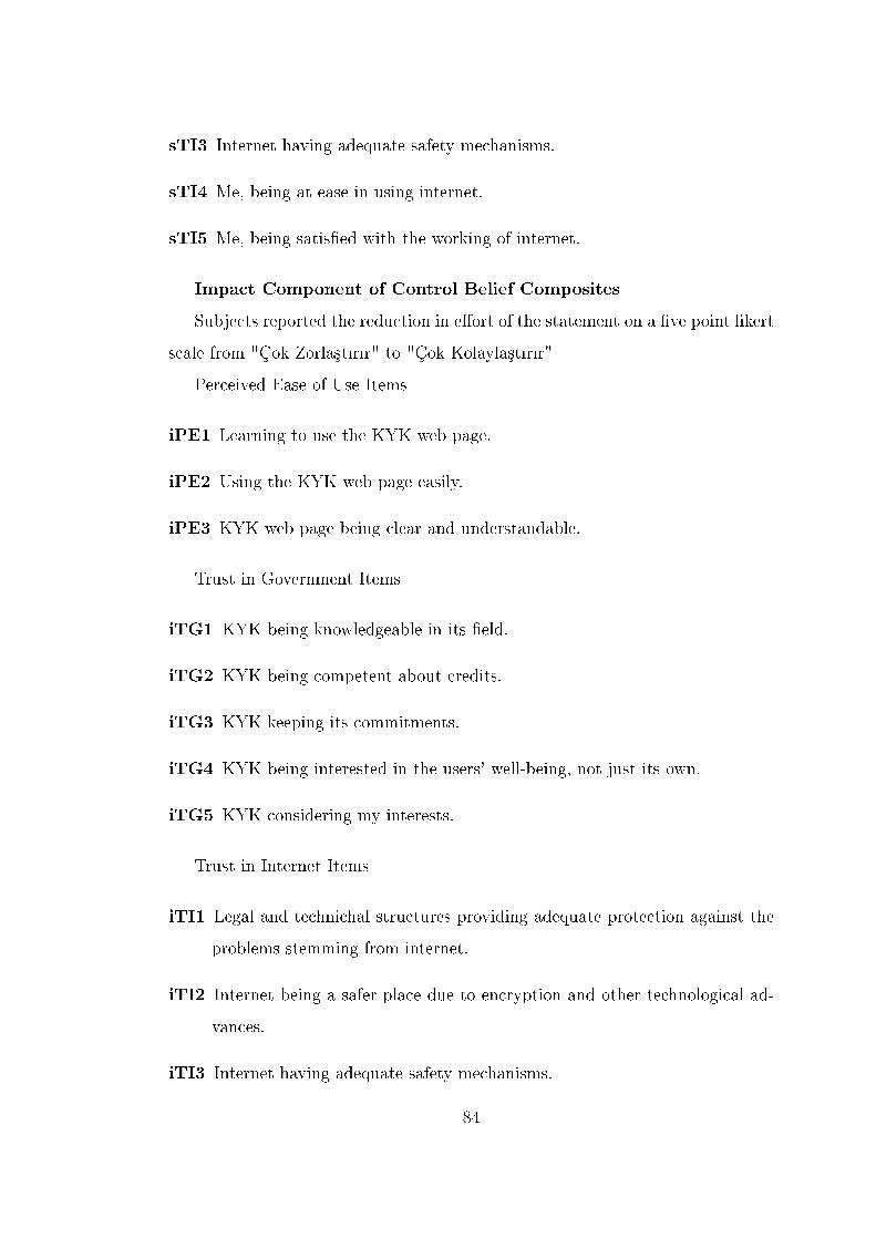
sTI3 Internet having adequate safety mechanisms.

sTI4 Me, being at ease in using internet.

sTI5 Me, being satis�ed with the working of internet.

Impact Component of Control Belief Composites

Subjects reported the reduction in e�ort of the statement on a �ve point likert

scale from "Çok Zorla³t�r�r" to "Çok Kolayla³t�r�r"

Perceived Ease of Use Items

iPE1 Learning to use the KYK web page.

iPE2 Using the KYK web page easily.

iPE3 KYK web page being clear and understandable.

Trust in Government Items

iTG1 KYK being knowledgeable in its �eld.

iTG2 KYK being competent about credits.

iTG3 KYK keeping its commitments.

iTG4 KYK being interested in the users' well-being, not just its own.

iTG5 KYK considering my interests.

Trust in Internet Items

iTI1 Legal and technichal structures providing adequate protection against the

problems stemming from internet.

iTI2 Internet being a safer place due to encryption and other technological ad-

vances.

iTI3 Internet having adequate safety mechanisms.

84

iTI4 Being at ease in using internet.

iTI5 Internet working in a satisfactory fashion.

Skills Items

iSK1 Having enough computer skills to match my needs.

iSK2 Being able to solve the problems I face using a computer.

Access Items

iAC1 Having access to a computer easily when I need one.

iAC2 Having access to internet easily when I need it.

85

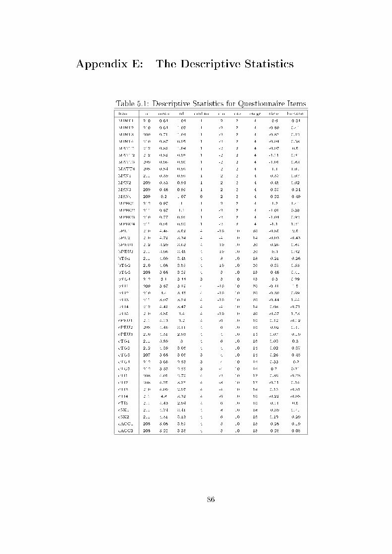
Appendix E: The Descriptive Statistics

Table 5.1: Descriptive Statistics for Questionnaire ItemsItem n mean sd median min max range skew kurtosis

MINT1 210 0.64 1.04 1 -2 2 4 -0.6 -0.34

MINT2 210 0.64 1.03 1 -2 2 4 -0.89 0.41

MINT3 209 0.71 1.04 1 -2 2 4 -0.82 0.12

MINT4 210 0.87 0.95 1 -2 2 4 -0.94 0.58

MATT1 212 0.82 1.04 1 -2 2 4 -0.97 0.5

MATT2 212 0.82 0.98 1 -2 2 4 -1.11 0.91

MATT3 209 0.96 0.96 1 -2 2 4 -1.01 0.83

MATT4 208 0.84 0.99 1 -2 2 4 -1.1 1.01

MSN1 211 0.59 0.99 1 -2 2 4 -0.57 0.07

MSN2 209 0.53 0.94 1 -2 2 4 -0.45 0.02

MSN3 209 0.46 0.99 1 -2 2 4 -0.37 -0.24

MSN4 209 0.2 1.07 0 -2 2 4 -0.23 -0.49

MPBC1 212 0.97 1 1 -2 2 4 -1.2 1.41

MPBC2 211 0.87 1.1 1 -2 2 4 -1.01 0.38

MPBC3 210 0.77 0.96 1 -2 2 4 -1.04 0.92

MPBC4 211 0.91 0.99 1 -2 2 4 -1.1 1.21

bPU1 210 4.46 3.52 4 -10 10 20 -0.85 2.5

bPU2 210 4.72 3.34 4 -4 10 14 -0.03 -0.43

bPEU1 212 3.29 3.62 4 -10 10 20 -0.26 0.84

bPEU2 211 3.96 3.45 4 -10 10 20 -0.3 0.92

bTG1 211 4.09 3.45 4 -8 10 18 -0.21 -0.26

bTG2 210 4.08 3.59 4 -10 10 20 -0.37 0.55

bTG3 208 3.68 3.29 4 -8 10 18 -0.46 0.41

bTG4 212 3.1 3.44 3 -8 10 18 -0.3 0.29

bTI1 209 3.87 3.19 4 -10 10 20 -0.41 1.5

bTI2 210 4.4 3.43 4 -10 10 20 -0.39 0.69

bTI3 211 3.97 3.24 4 -10 10 20 -0.44 1.44

bTI4 212 4.42 3.47 4 -4 10 14 0.08 -0.71

bTI5 210 3.85 3.4 4 -10 10 20 -0.57 1.73

cPEU1 211 4.13 3.2 4 -6 10 16 0.12 -0.12

cPEU2 208 4.46 3.11 4 -6 10 16 -0.02 0.31

cPEU3 210 4.51 2.93 4 -4 10 14 0.07 -0.19

cTG1 211 3.89 3 4 -6 10 16 0.03 0.3

cTG2 212 4.39 3.06 4 -4 10 14 0.02 -0.37

cTG3 207 3.68 3.06 3 -4 10 14 0.26 -0.45

cTG4 212 3.66 2.83 3 -4 10 14 0.33 -0.2

cTG5 212 3.33 2.88 3 -4 10 14 0.2 0.21

cTI1 208 4.01 2.79 4 -2 10 12 0.36 -0.28

cTI2 208 4.25 3.28 4 -8 10 18 -0.11 0.14

cTI3 210 4.09 2.97 4 -4 10 14 0.15 -0.31

cTI4 211 4.8 3.32 4 -6 10 16 -0.22 -0.08

cTI5 211 4.43 2.94 4 -6 10 16 -0.11 0.5

cSK1 211 4.74 3.41 4 -8 10 18 -0.39 0.71

cSK2 211 4.51 3.13 4 -6 10 16 0.19 -0.29

cACC1 208 5.08 3.59 4 -8 10 18 -0.28 -0.19

cACC2 208 5.22 3.36 4 -8 10 18 -0.25 -0.05

86

Appendix F: The Raw Data

87

Table5.2:

CorrelationsAmongQuestionn

aire

Item

sPredictorVariables

BehavioralBeliefComposites

ControlBeliefComposites

Intention

Attitute

SubjectiveNorm

Perc.Beh.Con.

P.U.

P.E.U.

Trustin

Gov.

Trustin

Internet

P.E.U.

Trustin

Government

Trustin

Internet

Skill

Access

IN1IN

2IN

3IN

4AT1AT2AT3ATT4SN1SN2SN3SN4PC1PC2PC3PC4PU1PU2PE1PE2TG1TG2TG3TG4TI1

TI2

TI3

TI4

TI5

PE1PE2PE3TG1TG2TG3TG4TG5TI1

TI2

TI3

TI4

TI5

SK1SK2AC1AC2

IN1

10.670.820.680.640.660.59

0.71

0.520.490.570.53

0.450.400.520.410.280.300.140.12

0.06

0.070.190.110.110.130.170.110.140.130.150.190.140.160.240.130.110.120.150.060.100.130.280.200.120.26

IN2

0.67

10.690.600.600.600.54

0.64

0.500.450.470.53

0.460.410.560.380.370.160.210.22

0.07

0.070.200.100.230.170.080.170.270.130.110.110.080.200.160.090.130.140.150.130.210.110.270.240.210.29

IN3

0.820.69

10.720.660.700.63

0.78

0.550.500.530.51

0.470.550.520.520.310.300.180.23

0.12

0.120.190.150.150.220.220.180.180.210.220.240.170.220.250.150.140.210.260.130.200.180.310.270.190.32

IN4

0.680.600.72

10.700.760.68

0.70

0.560.580.480.49

0.500.540.560.540.360.380.210.26

0.17

0.180.230.190.240.300.220.230.150.210.170.270.140.220.290.250.200.300.290.190.200.160.310.210.190.25

AT1

0.640.600.660.70

10.850.75

0.68

0.580.620.400.57

0.600.550.700.530.300.320.120.22

0.08

0.200.200.100.220.200.170.170.070.170.190.170.120.210.230.190.160.280.250.130.150.130.260.200.200.26

AT2

0.660.600.700.760.85

10.82

0.70

0.590.640.500.51

0.630.560.690.540.350.370.190.28

0.13

0.200.200.170.240.250.210.200.140.270.230.290.150.230.230.240.150.280.240.140.170.210.340.240.240.36

AT3

0.590.540.630.680.750.82

10.59

0.520.630.410.51

0.560.550.560.450.300.310.160.24

0.10

0.160.220.130.260.240.210.180.110.170.160.200.040.180.180.180.130.260.250.180.150.190.240.150.150.25

AT4

0.710.640.780.700.680.700.59

10.570.530.550.53

0.510.510.600.510.340.380.270.29

0.18

0.210.300.220.250.280.300.220.250.280.290.270.200.240.290.190.210.240.300.190.200.260.340.280.230.35

SN1

0.520.500.550.560.580.590.52

0.57

10.480.490.57

0.470.390.420.460.210.170.250.21

0.08

0.180.210.140.140.110.190.130.190.180.180.090.130.220.170.110.180.190.160.110.180.150.240.170.14

0.2

SN2

0.490.450.500.580.620.640.63

0.53

0.48

10.480.59

0.400.380.500.400.160.200.090.16

0.08

0.200.140.120.140.090.110.210.110.150.110.160.070.120.110.090.090.230.140.090.150.150.240.090.070.26

SN3

0.570.470.530.480.400.500.41

0.55

0.490.48

10.51

0.410.410.380.370.180.260.130.14

0.08

0.160.130.100.060.120.050.090.140.210.180.220.170.190.210.210.140.120.070.010.190.210.270.200.140.33

SN4

0.530.530.510.490.570.510.51

0.53

0.570.590.51

10.440.480.530.420.160.250.090.13-0.020.080.090.070.080.010.080.100.150.130.150.140.040.040.080.080.140.150.100.040.080.150.170.170.07

0.2

PC1

0.450.460.470.500.600.630.56

0.51

0.470.400.410.44

10.630.690.700.260.260.230.21

0.07

0.150.080.080.130.130.110.140.140.250.280.330.170.190.190.160.180.240.230.140.240.270.370.290.250.32

PC2

0.400.410.550.540.550.560.55

0.51

0.390.380.410.48

0.63

10.630.610.230.310.170.21

0.07

0.170.100.090.090.140.090.140.080.280.270.260.150.150.230.180.140.170.260.110.240.180.250.210.180.28

PC3

0.520.560.520.560.700.690.56

0.60

0.420.500.380.53

0.690.63

10.620.280.330.160.16

0.05

0.130.080.060.120.060.080.170.140.280.290.310.170.180.210.190.200.280.210.150.240.230.350.270.210.36

PC4

0.410.380.520.540.530.540.45

0.51

0.460.400.370.42

0.700.610.62

10.330.320.250.34

0.19

0.320.170.180.160.160.150.240.190.310.380.370.280.260.270.260.310.350.220.150.270.300.350.250.310.34

PU1

0.280.370.310.360.300.350.30

0.34

0.210.160.180.16

0.260.230.280.33

10.660.590.67

0.57

0.520.520.470.580.560.350.590.610.370.490.510.480.460.410.430.420.370.470.400.500.500.420.530.500.49

PU2

0.300.160.300.380.320.370.31

0.38

0.170.200.260.25

0.260.310.330.320.66

10.500.54

0.51

0.540.440.490.450.500.450.500.400.500.560.590.480.390.410.450.420.420.370.310.450.540.420.440.390.43

PE1

0.140.210.180.210.120.190.16

0.27

0.250.090.130.09

0.230.170.160.250.590.50

10.73

0.53

0.540.600.610.580.520.380.480.590.450.530.490.510.400.440.400.530.340.400.370.360.400.410.480.310.28

PE2

0.120.220.230.260.220.280.24

0.29

0.210.160.140.13

0.210.210.160.340.670.540.73

10.56

0.550.610.670.630.590.370.470.610.450.590.540.500.420.490.480.520.430.390.330.300.420.370.460.380.36

TG1

0.060.070.120.170.080.130.10

0.18

0.080.080.08-0.020.070.070.050.190.570.510.530.56

10.720.680.630.550.590.470.480.530.350.420.410.660.550.470.420.430.340.390.350.320.440.370.460.330.34

TG2

0.070.070.120.180.200.200.16

0.21

0.180.200.160.08

0.150.170.130.320.520.540.540.55

0.72

10.610.610.500.540.390.450.430.420.440.420.600.620.420.480.480.310.360.350.330.450.310.410.340.32

TG3

0.190.200.190.230.200.200.22

0.30

0.210.140.130.09

0.080.100.080.170.520.440.600.61

0.68

0.61

10.700.660.600.540.430.570.460.460.410.570.530.670.540.560.430.460.450.290.460.410.480.390.43

TG4

0.110.100.150.190.100.170.13

0.22

0.140.120.100.07

0.080.090.060.180.470.490.610.67

0.63

0.610.70

10.620.600.520.460.570.450.450.500.540.440.520.560.600.330.400.380.260.410.340.470.270.31

TI1

0.110.230.150.240.220.240.26

0.25

0.140.140.060.08

0.130.090.120.160.580.450.580.63

0.55

0.500.660.62

10.740.570.470.490.390.410.450.390.400.530.550.470.650.600.610.320.390.330.410.390.33

TI2

0.130.170.220.300.200.250.24

0.28

0.110.090.120.01

0.130.140.060.160.560.500.520.59

0.59

0.540.600.600.74

10.640.520.520.320.390.420.440.440.390.440.400.470.680.610.360.350.310.400.350.28

TI3

0.170.080.220.220.170.210.21

0.30

0.190.110.050.08

0.110.090.080.150.350.450.380.37

0.47

0.390.540.520.570.64

10.480.490.370.410.410.400.400.440.380.420.500.630.650.320.440.430.380.360.39

TI4

0.110.170.180.230.170.200.18

0.22

0.130.210.090.10

0.140.140.170.240.590.500.480.47

0.48

0.450.430.460.470.520.48

10.630.390.410.400.420.400.320.330.400.420.500.510.670.530.550.570.590.55

TI5

0.140.270.180.150.070.140.11

0.25

0.190.110.140.15

0.140.080.140.190.610.400.590.61

0.53

0.430.570.570.490.520.490.63

10.320.380.400.480.420.390.300.520.290.450.450.460.620.490.580.430.49

PE1

0.130.130.210.210.170.270.17

0.28

0.180.150.210.13

0.250.280.280.310.370.500.450.45

0.35

0.420.460.450.390.320.370.390.32

10.630.640.550.480.530.570.510.550.390.370.460.590.600.550.560.63

PE2

0.150.110.220.170.190.230.16

0.29

0.180.110.180.15

0.280.270.290.380.490.560.530.59

0.42

0.440.460.450.410.390.410.410.380.63

10.720.550.470.480.470.490.550.430.350.520.690.490.470.53

0.6

PE3

0.190.110.240.270.170.290.20

0.27

0.090.160.220.14

0.330.260.310.370.510.590.490.54

0.41

0.420.410.500.450.420.410.400.400.640.72

10.560.470.430.580.510.550.500.420.510.660.570.570.570.58

TG1

0.140.080.170.140.120.150.04

0.20

0.130.070.170.04

0.170.150.170.280.480.480.510.50

0.66

0.600.570.540.390.440.400.420.480.550.550.56

10.710.630.570.660.420.460.410.340.500.460.540.470.47

TG2

0.160.200.220.220.210.230.18

0.24

0.220.120.190.04

0.190.150.180.260.460.390.400.42

0.55

0.620.530.440.400.440.400.400.420.480.470.470.71

10.620.600.610.380.500.430.380.540.490.480.490.52

TG3

0.240.160.250.290.230.230.18

0.29

0.170.110.210.08

0.190.230.210.270.410.410.440.49

0.47

0.420.670.520.530.390.440.320.390.530.480.430.630.62

10.680.680.550.530.430.330.480.450.470.380.45

TG4

0.130.090.150.250.190.240.18

0.19

0.110.090.210.08

0.160.180.190.260.430.450.400.48

0.42

0.480.540.560.550.440.380.330.300.570.470.580.570.600.68

10.690.590.560.520.360.490.440.470.440.48

TG5

0.110.130.140.200.160.150.13

0.21

0.180.090.140.14

0.180.140.200.310.420.420.530.52

0.43

0.480.560.600.470.400.420.400.520.510.490.510.660.610.680.69

10.490.510.510.340.550.480.500.440.44

TI1

0.120.140.210.300.280.280.26

0.24

0.190.230.120.15

0.240.170.280.350.370.420.340.43

0.34

0.310.430.330.650.470.500.420.290.550.550.550.420.380.550.590.49

10.640.630.440.530.470.400.490.46

TI2

0.150.150.260.290.250.240.25

0.30

0.160.140.070.10

0.230.260.210.220.470.370.400.39

0.39

0.360.460.400.600.680.630.500.450.390.430.500.460.500.530.560.510.64

10.800.460.470.490.510.460.45

TI3

0.060.130.130.190.130.140.18

0.19

0.110.090.010.04

0.140.110.150.150.400.310.370.33

0.35

0.350.450.380.610.610.650.510.450.370.350.420.410.430.430.520.510.630.80

10.460.440.480.480.490.41

TI4

0.100.210.200.200.150.170.15

0.20

0.180.150.190.08

0.240.240.240.270.500.450.360.30

0.32

0.330.290.260.320.360.320.670.460.460.520.510.340.380.330.360.340.440.460.46

10.600.560.580.650.59

TI5

0.130.110.180.160.130.210.19

0.26

0.150.150.210.15

0.270.180.230.300.500.540.400.42

0.44

0.450.460.410.390.350.440.530.620.590.690.660.500.540.480.490.550.530.470.440.60

10.610.620.60

0.7

SK1

0.280.270.310.310.260.340.24

0.34

0.240.240.270.17

0.370.250.350.350.420.420.410.37

0.37

0.310.410.340.330.310.430.550.490.600.490.570.460.490.450.440.480.470.490.480.560.61

10.730.610.71

SK2

0.200.240.270.210.200.240.15

0.28

0.170.090.200.17

0.290.210.270.250.530.440.480.46

0.46

0.410.480.470.410.400.380.570.580.550.470.570.540.480.470.470.500.400.510.480.580.620.73

10.610.64

AC1

0.120.210.190.190.200.240.15

0.23

0.140.070.140.07

0.250.180.210.310.500.390.310.38

0.33

0.340.390.270.390.350.360.590.430.560.530.570.470.490.380.440.440.490.460.490.650.600.610.61

10.77

AC2

0.260.290.320.250.260.360.25

0.35

0.200.260.330.20

0.320.280.360.340.490.430.280.36

0.34

0.320.430.310.330.280.390.550.490.630.600.580.470.520.450.480.440.460.450.410.590.700.710.640.77

1

88