e = fx x hw f +++ w f w f e - university of notre damecoast/jjwteach/www/www/30125/... · •in...

CE 30125 - Lecture 16

p. 16.1

LECTURE 16

GAUSS QUADRATURE

• In general for Newton-Cotes (equispaced interpolation points/ data points/ integrationpoints/ nodes).

84

• Note that for Newton-Cotes formulae only the weighting coefficients were unknownand the were fixed

f x xd

xS

xE

h w'o fo w'1 f1 w'N fN+ + + E+=

f0

f1f2

fN

h

= x0xs x1 x2 = xNxE

closed formula

wi

xi


p. 16.2

• However the number of and placement of the integration points influences the accuracyof the Newton-Cotes formulae:

• even degree interpolation function exactly integrates an degree poly-nomial This is due to the placement of one of the data points.

• odd degree interpolation function exactly integrates an degree polyno-mial.

• Concept: Let’s allow the placement of the integration points to vary such that wefurther increase the degree of the polynomial we can integrate exactly for a givennumber of integration points.

• In fact we can integrate an degree polynomial exactly with only integra-tion points

N Nth N 1+ th

N Nth Nth

2N 1+ N 1+


p. 16.3

• Assume that for Gauss Quadrature the form of the integration rule is

85

• In deriving (not applying) these integration formulae

• Location of the integration points, are unknown

• Integration formulae weights, are unknown

• unknowns we will be able to exactly integrate any degree polyno-mial!

f x xdxS

xE

wo fo w1 f1 wN fN+ + + E+=

f0

f1

f2

fN

x0xs x1 x2 xN xE

f3

x3

xi i O N=

wi i O N=

2 N 1+ 2N 1+


p. 16.4

Derivation of Gauss Quadrature by Integrating Exact Polynomials and Matching

Derive 1 point Gauss-Quadrature

• 2 unknowns , which will exactly integrate any linear function

• Let the general polynomial be

where the coefficients can equal any value

• Also consider the integration interval to be such that and (noloss in generality since we can always transform coordinates).

• Substituting in the form of

wo xo

f x Ax B+=

A B

1 + 1– xS 1–= xE + 1=

f x xd

1–

+ 1

wo f xo =

f x

Ax B+ xd

1–

+ 1

wo Axo B+ =


p. 16.5

• In order for this to be true for any 1st degree polynomial (i.e. any and ).

• Therefore , for 1 point Gauss Quadrature. 86

• We can integrate exactly with only 1 point for a linear function while for Newton-Coteswe needed two points!

Ax2

2----- Bx+

+ 1

1–wo Axo B+ =

A 0 B 2 + A xowo B wo +=

A B

0 xowo=

2 wo =

xo 0= wo 2= N 1=

f0f(x)

x0-1 +1


p. 16.6

Derive a 2 point Gauss Quadrature Formula 87

• The general form of the integration formula is

• , , , are all unknowns

• 4 unknowns we can fit a 3rd degree polynomial exactly

• Substituting in for into the general form of the integration rule

x0 x1-1 +1

I wo fo w1 f1+=

wo xo w1 x1

f x Ax3 Bx2 Cx D+ + +=

f x

f x xd

1–

+ 1

wo f xo w1 f x1 +=


p. 16.7

• In order for this to be true for any third degree polynomial (i.e. all arbitrary coefficients,, , , ), we must have:

Ax3 Bx2 Cx D+ + + xd

1–

+ 1

wo Axo3

Bx2o Cxo D+ + + w1 Ax3

1 Bx21 Cx1 D+ + + +=

Ax4

4---------

Bx3

3---------

Cx2

2--------- Dx+ + +

+ 1

1–wo Ax3

o Bx2o Cxo D+ + + w1 Ax3

1 Bx21 Cx1 D+ + + +=

A wox3o w1x3

1+ B wox2o w1x2

123---–+ C woxo w1x1+ D wo w1 2–+ + + + 0=

A B C D

wox3o w1x3

1+ 0=

wox2o w1x2

123---–+ 0=

woxo w1x1+ 0=

wo w1 2–+ 0=


p. 16.8

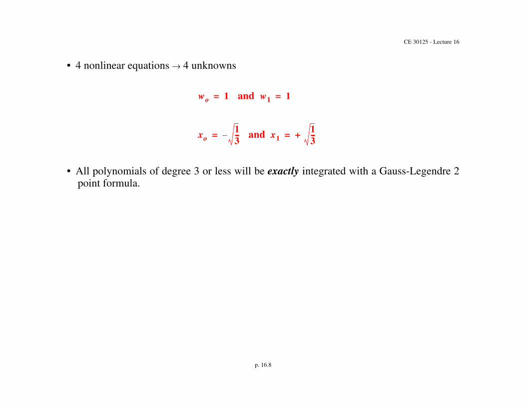
• 4 nonlinear equations 4 unknowns

and

and

• All polynomials of degree 3 or less will be exactly integrated with a Gauss-Legendre 2point formula.

wo 1= w1 1=

xo13---–= x1 + 1

3---=


p. 16.9

Gauss Legendre Formulae

,

0 1 0 2 1

1 2,

1, 1 3

2 3 -0.774597, 0, +0.774597

0.5555, 0.8889, 0.5555

5

I f x xd

1–

+1

wi fi

i 0=

N

E+= =

N N 1+xi

i 0 N=wi

Exact forpolynomials of

degree

13---– +

13---

N N 1+ 2N 1+


p. 16.10

,

3 4 -0.86113631-0.33998104 0.33998104 0.86113631

0.347854850.652145150.652145150.34785485

7

4 5 -0.90617985-0.53846931 0.00000000 0.53846931 0.90617985

0.236926890.478628670.568888890.478628670.23692689

9

5 6 -0.93246951-0.66120939-0.23861919 0.23861919 0.66120939 0.93246951

0.171324490.360761570.467913930.467913930.360761570.17132449

11

N N 1+xi

i 0 N=wi

Exact forpolynomials of

degree


p. 16.11

• Notes

• = the number of integration points

• Integration points are symmetrical on

• Formulae can be applied on any interval using a coordinatetransformation

• integration points will integrate polynomials of up to degree exactly.

• Recall that Newton Cotes integration points only integrates an degree polynomial exactly depending on being odd or even.

• For Gauss-Legendre integration, we allowed both weights and integration pointlocations to vary to match an integral exactly more d.o.f. allows you tomatch a higher degree polynomial!

• An alternative way of looking at Gauss-Legendre integration formulae is that weuse Hermite interpolation instead of Lagrange interpolation! (How can this besince Hermite interpolation involves derivatives let’s examine this!)

N 1+

1 +1–

N 1+ 2N 1+

N 1+

Nth/N 1th+ N


p. 16.12

Derivation of Gauss Quadrature by Integrating Hermite Interpolating Functions

Hermite interpolation formulae

• Hermite interpolation which matches the function and the first derivative at inter-polation points is expressed as:

88

• It can be shown that in general for non-equispaced points

N 1+

g x i x fi

i 0=

N

i x fi1

i 0=

N

+=

f0 f1 f2 fNf4

x0 x1 x2 x3

f0(1)

f1 f2(1)

f3 f3(1)

x4 x5

f4(1)

f5 f5(1)

fN(1)

xN

0 1 2 3 4 5 N

(1)

i x ti x liN x liN x = i 0 N=

i x si x liN x liN x = i 0 N=


p. 16.13

where

pN x x xo– x x1– x xN–

liN x p

Nx

x xi– p 1 N

xi --------------------------------------- i 0 N=

ti x 1 x xi– 2 liN1

xi –

si x x xi–


p. 16.14

Example of defining a cubic Hermite interpolating function

• Derive Hermite interpolating functions for 2 interpolation points located at and for the interval .

89

points

• Establish

1– + 11 + 1–

f0 f1

x0 = 1 x1 = +1

f0 (1)f1

(1)

x

N 1+ 2= N 1=

pN x

p1

x x xo– x x1– =

p 1 1

x x xo– x x1– +=


p. 16.15

• Establish

• Let

• Substitute in and

liN x

li1 x p1 x

x xi– p11

xi -----------------------------------------=

li1 x x xo– x x1–

x xi– xi xo– xi x1– + ---------------------------------------------------------------------=

i 0=

lo1 x x xo– x x1–

x xo– 0 xo x1– + ------------------------------------------------------=

lo1 x x x1–

xo x1–----------------=

xo 1–= x1 + 1 =

lo1 x 12--- 1 x– =


p. 16.16

• Let

• Substitute in values for ,

• Taking derivatives

i 1=

l11 x x xo– x x1–

x x1– x1 xo– 0+ ------------------------------------------------------=

xo x1

l11 x 12--- 1 x+ =

l1

o1x

12---–=

l1

11x +

12----=


p. 16.17

• Establish

• Establish

ti x

to x 1 x xo– 2l1

o1 xo –=

to x 1 x 1+ 2 – 12---–

=

to x 2 x+=

t1 x 1 x x1– 2 l1

11 x1 –=

t1 x 1 x 1– 212---

–=

t1 x 2 x–=

si x

so x x 1+=

s1 x x 1–=


p. 16.18

• Establish

i x

o x to x lo1 x lo1 x =

o x 2 x+ 12--- 1 x– 1

2--- 1 x– =

o x 14--- 2 3x– x3+ =

1 x t1 x l11 x l11 x =

1 x 2 x– 12--- 1 x+ 1

2--- 1 x+ =

1 x 14--- 2 3x x3–+ =


p. 16.19

• Establish

• In general

i x

o x so x lo1 x lo1 x =

o x x 1+ 12--- 1 x– 1

2--- 1 x– =

o x 14--- 1 x– x2– x3+ =

1 x s1 x l11 x l11 x =

1 x x 1– 12--- 1 x+ 1

2--- 1 x+ =

1 x 14--- 1– x– x2 x3+ + =

g x o x fo 1 x f1 o x f 1 o

1 x f 1 1

+ + +=


p. 16.20

90

• These functions satisfy the constraints

1

i(x)

1(x)0(x)

x

i(x)

0(x)

1(x)

x

i (x)

1 (x)

0 (x)

(1)

(1)

(1)

x

i (x)(1)

0 (1) (1)

x

i xj ij= 1 i

xj 0=

i xj 0= 1 i xj ij=


p. 16.21

Gauss-Legendre Quadrature by integrating Hermite interpolating polynomials

• Notes

• Use without loss of generality we can always transform the interval.

• Approximation for is exact for degree polynomials

• We can derive all Gauss-Legendre quadrature formulae by approximating with an degree Hermite interpolating function using specially selected integration/

interpolation points.

where

I f x xd

1–

+ 1

wi fi E+

i 0=

N

= =

1 +1–

I 2N 1+

f x 2N 1th+ N

I g x x E+d

1–

+ 1

=

g x i x fi

i 0=

N

i x fi1

i 0=

N

+=


p. 16.22

• Thus

where

and

• Furthermore we can show that

I i x fi

i 0=

N

i x fi1

i 0=

N

+

1–

+ 1

dx= E+

I Ai fi

i 0=

N

Bi fi1

i 0=

N

E+ +=

Ai i x xd

1–

+ 1

Bi i x xd

1–

+ 1

EpN 1+

2x

2N 2+ !----------------------- f

2N 2+ xo + H.O.T. xd

1–

+ 1

=


p. 16.23

• Note that we are assuming Taylor series expansions about and using higher orderterms in the expansion.

• Therefore for any polynomial of degree or less!

• The problem that we encounter is that the integration formula as it now stands ingeneral requires us to know both functional and first derivative values at the nodes!

• Let us select such that

xo

E 0= 2N 1+

xo x1 x2 xN

Bi 0= i 0 N=

i x xd

1–

+ 1

0= i 0 N=

si x liN x liN x xd

1–

+ 1

0= i 0 N=

x xi– pN x

x xi– pN1

xi ------------------------------------ liN x xd

1–

+ 1

0= i 0 N=


p. 16.24

polynomial of degree

polynomial of degree

• Therefore we require to be orthogonal on to all polynomials of degree or less any multiple of Legendre-Polynomials will satisfy this.

• Let

where

= the Legendre polynomial of degree

is required to normalize the leading coefficient of

1

pN1

xi ------------------ pN x liN x

1–

+ 1

dx 0= i 0 N=

pN x N 1+

liN x N

pN x 1 +1– N

pN x 2N 1+ N 1+ ! 2

2 N 1+ !-----------------------------------------PN 1+ x =

pN x x xo– x x1– x x2– x xN– =

PN 1+ N 1+

2N 1+ N 1+ ! 2

2 N 1+ !----------------------------------------- PN 1+ x


p. 16.25

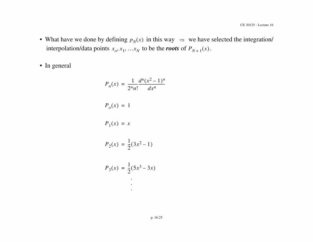
• What have we done by defining in this way we have selected the integration/interpolation/data points to be the roots of .

• In general

.

.

.

pN x xo x1 xN PN 1+ x

Pn x 12nn!----------

dn x2 1– n

dxn---------------------------=

Po x 1=

P1 x x=

P2 x 12--- 3x2 1– =

P3 x 12--- 5x3 3x– =


p. 16.26

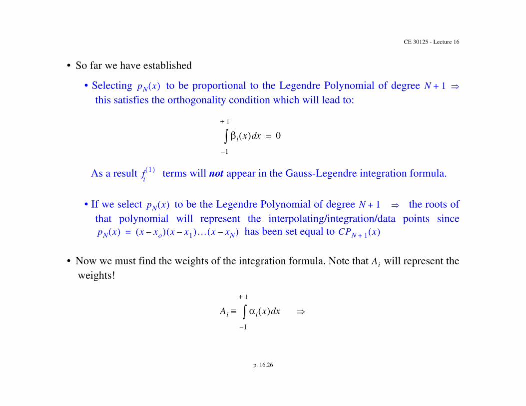
• So far we have established

• Selecting to be proportional to the Legendre Polynomial of degree this satisfies the orthogonality condition which will lead to:

As a result terms will not appear in the Gauss-Legendre integration formula.

• If we select to be the Legendre Polynomial of degree the roots ofthat polynomial will represent the interpolating/integration/data points since

has been set equal to

• Now we must find the weights of the integration formula. Note that will represent theweights!

pN x N 1+

i x xd

1–

+ 1

0=

f 1 i

pN x N 1+

pN x x xo– x x1– x xN– = CPN 1+ x

Ai

Ai i x xd

1–

+ 1


p. 16.27

where

and where are the roots of the Legendre polynomial of degree or

Ai ti x liN x liN x 1–

+ 1

= dx

ti x 1 x xi– 2 liN1

xi –=

liN x pN x

x xi– pN1

xi ------------------------------------=

pN x x xo– x xN– =

xo xN N 1+

pN x 2N 1+ N 1+ ! 2

2 N 1+ !-----------------------------------------PN 1+ x =


p. 16.28

Two point Gauss-Legendre integration

Develop a 2 point Gauss-Legendre integration formula for . Let

• Thus

1 +1–

g x i x fi

j 0=

1

i x fi1

j 0=

1

+=

g x o x fo 1 x f1 o x fo1 1 x f1

1 + + +=

I g x x E+d

1–

+ 1

=

I o x fo xd

1–

+1

1 x f1 xd

1–

+1

o x fo1

xd

1–

+1

1 x f11

xd

1–

+1

+ + +=

I fo o x xd

1–

+1

f1 1 x xd

1–

+1

fo1 o x xd

1–

+1

f11 1 x xd

1–

+1

+ + +=


p. 16.29

Step 1 - Establish interpolating points

• Interpolation points will be the roots of the Legendre Polynomial of order 2.

P2 x 12--- 3x2 1– =

12--- 3x2 1– 0=

3x2 1=

x2 13---=

x0 113---=

x0 1 0.57735=


p. 16.30

• Checking these roots

P2 x 1222!----------

d2 x2 1– 2

dx2---------------------------=

P2 x 18---

d2

dx2-------- x4 2x2– 1+ =

P2 x 18--- 12x2 4– =

P2 x 12--- 3x2 1– =

p1 x 22 2! 2

2 2 !------------------ P2 x =

p1 x 4 44 3 2 ------------------

12--- 3x2 1– =

p1 x x2 13---–=


p. 16.31

• From formula which defines using the integration points

Step 2 - Establish the coefficients of the derivative terms in the integration formula

• Let’s demonstrate that with the roots we will satisfy

and

• First develop and by developing

p1 x

p1 x x13---+

x13---–

x2 13---–= =

xo 1 0.57735=

o x 1–

+ 1

dx 0= 1 x xd

1–

+ 1

0=

o x 1 x p1 x , p11

x , lo1 x , l11 x , so x and s1 x

p1 x x xo– x x1– =

p11

x x xo– x x1– +=


p. 16.32

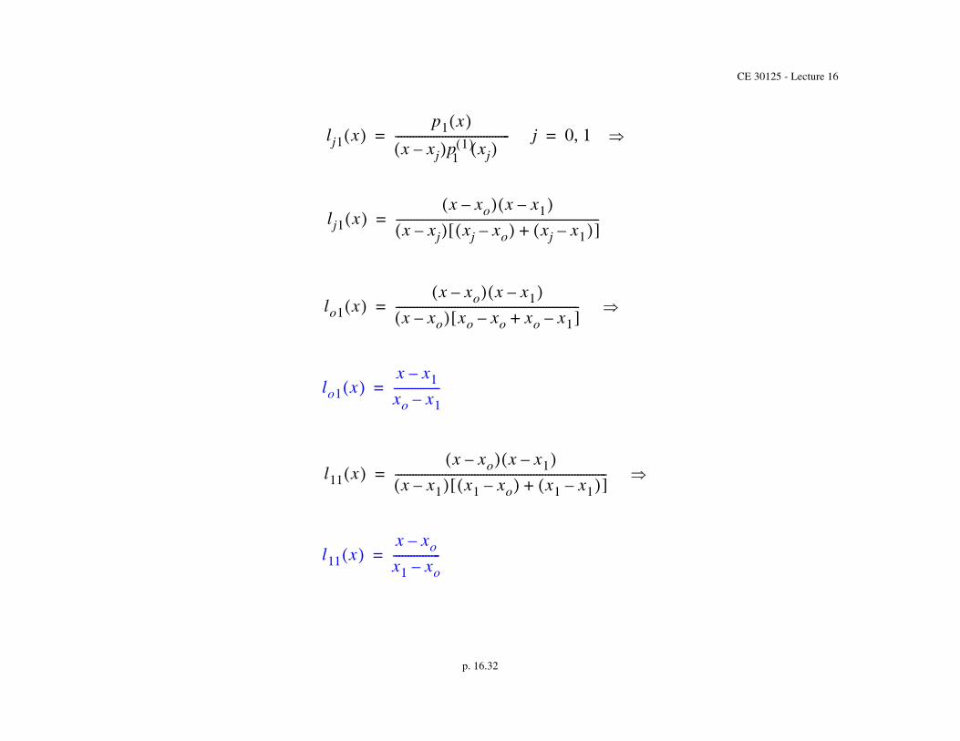
lj1 x p1 x

x xj– p 1 1

xj ---------------------------------------= j 0 1=

lj1 x x xo– x x1–

x xj– xj xo– xj x1– + ---------------------------------------------------------------------=

lo1 x x xo– x x1–

x xo– xo xo– xo x1–+ --------------------------------------------------------------=

lo1 x x x1–

xo x1–----------------=

l11 x x xo– x x1–

x x1– x1 xo– x1 x1– + ------------------------------------------------------------------------=

l11 x x xo–

x1 xo–----------------=


p. 16.33

• Now we can establish

• Noting that ,

so x x xo–=

s1 x x x1–=

o x

o x so x lo1 x lo1 x =

o x x xo– x x1–

xo x1–---------------- x x1–

xo x1–---------------- =

xo13---–= x1

13---=

o x x13---+

=x

13---–

x13---–

13---–

13---–

2

-------------------------------------------

o x 34--- x3 1

3---x2 1

3---x–

13--- 3 2/

+–=


p. 16.34

• Similarly for

• Substituting ,

1 x

1 x s1 x l11 x l11 x =

1 x x x1– x xo– x1 xo–

---------------------x xo– x1 xo–

---------------------=

xo13---–= x1

13---=

1 x x

13---–

x13---+

x13---+

13---

13---+

2

------------------------------------------------------------------=

1 x 34--- x3 1

3---x2 1

3---x–

13--- 3 2/

–+=


p. 16.35

• Now we can develop

o x xd1–

+1

o x xd1–

+1

34--- x3 1

3---x2–

13---x–

13--- 3 2/

+ xd1–

+1

=

o x xd1–

+1

34---

x4

4-----

13--- 3 2/

x3–16---x2–

13--- 3 2/

x++1

1–=

o x xd1–

+1

34---

14---

13--- 3 2/

–16---–

13--- 3 2/

+ 1

4---

13--- 3 2/ 1

6---–

13--- 3 2/

–+ –=

o x xd1–

+1

0=


p. 16.36

• Develop

1 x xd1–

+1

1 x xd1–

+1

34--- x3 1

3---x2 1

3---x–

13--- 3 2/

–+ xd1–

+1

=

1 x xd1–

+1

34---

x4

4-----

13--- 3 2/

x3 16---x2–

13--- 3 2/

x–++1

1–=

1 x xd1–

+1

34---

14---

13--- 3 2/ 1

6---–

13--- 3 2/

–+ 1

4---

13--- 3 2/

–16---–

13--- 3 2/

+ –=

1 x xd1–

+1

0=


p. 16.37

• Now our integration formula reduces to:

where

and

Step 3 - Develop ,

• Establish

I fo o x x f1 1 x xd1–

+1

+d1–

+1

=

I Aofo A1f1+=

Ao o x xd1–

+1

A1 1 x xd1–

+1

Ao A1

o x

o x to x lo1 x lo1 x =

o x 1 x xo– 2lo11

xo – lo1 x lo1 x =


p. 16.38

o x 1 x xo– 2xo x1–----------------–

x x1–

xo x1–---------------- x x1–

xo x1–---------------- =

o x 1 x13---+

2

13---–

13---–

-------------------------–

x

13---–

x13---–

13---–

13---–

13---–

13---–

--------------------------------------------------------------=

o x 34--- 1 x

13---+

2

213---–

--------------

–

x2 213---x–

13---+

=

o x 3 34

----------2

3------- x+

x2 213---x–

13---+

=

o x 34--- 3 x3 x– 2

13--- 3 2/

+

=


p. 16.39

• Develop

o x xd1–

+1

o x xd1–

+1

34--- 3 x3 x– 2

13--- 3 2/

+

1–

+1

dx=

o x xd1–

+1

34--- 3

x4

4-----

x2

2-----– 2

13--- 3 2/

+ x+1

1–=

o x xd1–

+1

34--- 3=

14---

12---– 2

13--- 3 2/

+ 1

4---

12---– 2

13--- 3 2/

– –

o x xd1–

+1

34--- 3 4

13---

13---

=

o x xd1–

+1

1=

Ao 1=


p. 16.40

• Similarly we can show that

• Thus we have established the two point Gauss Quadrature rule

where and are the integration points and

• We note that this integration rule was established by defining a Hermite cubic interpo-lating function and defining the integration points , such that

and

• Therefore the functional derivative values drop out of the Gauss Legendre integra-tion formula!

A1 1 x xd1–

+1

1= =

I f x xd1–

+1

wo fo w1 f1+= =

xo13---–= x1 +

13---= wo w1 1= =

xo x1

o x xd1–

+1

0= 1 x xd1–

+1

0=

e = fx x hw f +++ w f w f e - university of notre damecoast/jjwteach/www/www/30125/... · •in...

Documents