e ects of parental absence on child labor and school ... · e ects of parental absence on child...
TRANSCRIPT

Effects of Parental Absence on Child Labor andSchool Attendance in the Philippines
Claus C Portner∗
Department of EconomicsAlbers School of Business and Economics
Seattle University, Pigott 502901 12th AvenueP.O. Box 222000
Seattle, WA 98122Ph: +1 206-651-4151
&Center for Studies in Demography and Ecology
University of Washington
September 2014
∗I would like to thank Robert E. Evenson for access to the data set and for his answers to numerous ques-tions. I would also like to thank three anonymous referees, Mark Pitt, John Strauss, and Finn Tarp for theirhelpful comments and suggestions. Partial support for this research came from a Eunice Kennedy ShriverNational Institute of Child Health and Human Development research infrastructure grant, 5R24HD042828,to the Center for Studies in Demography and Ecology at the University of Washington. This paper is asubstantially revised version of Chapter 4 in my PhD thesis and was previously circulated under the title“Children’s Time Allocation in the Laguna Province, the Philippines.”

Abstract
This paper uses longitudinal data from the Philippines to analyze determinants of
children’s time allocation. The estimation method takes into account both the simul-
taneity of time use decisions, by allowing for correlation of residuals across time uses,
and unobservable family heterogeneity, through the inclusion of household fixed effects.
Importantly, this improved estimation method leads to different results than when ap-
plying the methods previously used in the literature. Girls suffer significantly from the
absence of their mother with a reduction in time spent in school that is equivalent to
dropping out completely. This effect is substantially larger when controlling for house-
hold unobservables than when not. Boys increase time spent working on market related
activities in response to an absent father, although this time appears to come out of
leisure rather than school or doing household chores. Land ownership substantially
increase the time boys spend on school activities, whereas renting land reduces the
time girls spend on school. Finally, there does not appear to be a substantial trade-off
between time spent on school and work, either in the market or at home.
1

1 Introduction
A child’s time may be spent on any number of activities, and the distribution across different
activities has implications both for the child’s current well-being and for its future prospects.
Parents’ decisions about how much time a child spends on schooling, working, doing domestic
work, or on leisure activities directly impact the child’s current utility. This may also have
large impacts on the child’s human capital accumulation, with a resulting indirect impact
on the development of the society.1 This paper aims to answer two questions. First, how are
different time uses traded off against each other? Second, to what extent are these trade-
offs the result of observable conditions, that may potentially be changed, or the result of
unobservable individual or household characteristics that are more difficult to impact? Focus
is especially on how parental absence affect the allocation of children’s time across different
time uses.
The determinants of children’s time allocation have attracted significant public interest.
In response, since the early 1990s, there has been a substantial increase in the amount of
research on the time allocation of children in developing countries (Edmonds 2008). One
of the main difficulties in understanding the trade-off between different uses of children’s
time is that the uses are jointly determined. The initial research on the trade-off between
work and schooling ignored this issue and found that working caused substantial negative
effects on school attendance, grade progression, human capital accumulation, and educational
attainment (Patrinos and Psacharopoulos 1995; Akabayashi and Psacharopoulos 1999; Heady
2003).
The later literature has predominantly employed one of two methods to address the issues
of joint determination of time use: instrumental variables (IV) or some type of exogenous
variation in conditions. The main problem with the instrumental variables method is that it
1An example is hard or hazardous work that may have damaging effects on children’s health that areonly seen later in life. The improper use of pesticides may, for example, have serious adverse health effectsthat only emerge following a long time lag. Another example is the human capital accumulation of the child,which is a strong predictor of lifetime income.
2
requires one or more variables that affect, say, work but do not affect schooling, or vice versa.
In addition, the results hold only for the subset of children who change behavior because of
the instrument. This may explain why the IV results have been mixed, with some finding
a stronger association between work and schooling and others finding a much weaker asso-
ciation as compared to the prior literature (Boozer and Suri 2001; Rosati and Rossi 2003;
Ray and Lancaster 2004; Gunnarsson, Orazem, and Sanchez 2006). The other approach
exploits changes in local conditions when examining the relationship between schooling and
work, such as changes in laws or programs that affect the relative cost of going to school.
Using this approach, the general finding is that there has been a substantially larger in-
crease in schooling than there has been a decrease in market work (Ravallion and Wodon
2000; Arends–Kuenning and Amin 2004; Cardoso and Souza 2004; Kazianga, Walque, and
Alderman 2009; de Hoop and Rosati 2012).2
Another strand of the literature has tried to understand the medium- and long-term
impact of working on human capital and future earnings. The earlier literature found that
individuals who began work at a younger age tended to have lower earnings as adults,
except for those with no education, perhaps because of the accumulation of experience (Ilahi,
Orazem, and Sedlacek 2005; Emerson and Souza 2011). More recent studies with a stronger
focus on controlling for unobservable characteristics that might influence both later wages
and the time use decision when young, have found negligible or even positive effects on
outcomes such as test scores and earnings (Beegle, Dehejia, and Gatti 2009; Dumas 2012).
With focus primarily on child labor and schooling, domestic work has received relatively
little attention (Edmonds 2008). Domestic work is, however, an important time use and
should not be ignored, especially with respect to girls (Assaad, Levison, and Zibani 2010).
It has been argued that whether or not there is a trade-off between school and work depends
on whether or not domestic work is included, especially for girls (Levison and Moe 1998;
Levison, Moe, and Marie Knaul 2001). This result is, however, not uniformly supported
2A similar result holds for increased proximity to schools (Kondylis and Manacorda 2012; de Hoop andRosati 2012).
3

(de Hoop and Rosati 2012). In the same vein, the prior research has paid little attention to
leisure, despite the potential importance of leisure on a child’s development and his or her
ability to perform satisfactorily in school (Edmonds 2008).
Most of the prior research has mainly examined the participation decision, rather the
number of hours spent on each (Edmonds 2008). To the extent that researchers have ex-
amined work and schooling jointly, the commonly-used method has been bivariate probit.
This approach, however, has a number of potential issues, both in terms of evaluating the
effects of explanatory variables and in attempting to control for unobserved characteristics
(Edmonds 2008). In addition, incorporating the decision on domestic work would require
the implementation of a trivariate probit, which is not straightforward.
This paper makes three main contributions to the literature. First, it incorporates all
possible time uses for a child—schooling, market work, domestic work, and leisure—using a
data set with detailed information on children’s time use over the week prior to the survey,
measured over two survey rounds.
Second, it takes into account family heterogeneity and potentially endogenous variables
through the use of household fixed effects. The two survey rounds provide enough variation
within households and across time to estimate household fixed effects. Most of the literature
have relied on cross-sectional data and have therefore either ignored the role of unobserved
family heterogeneity or used an IV approach to deal with endogenous variables. This is
especially important when estimating the effects of factors such as parental absence that are
likely to be correlated with unobservable household characteristics and therefore biased in
standard OLS estimates.
Third, it takes seriously the joint nature of time allocation decisions. It models all
four time uses jointly and makes use of the available time data instead of just focusing on
the participation decision (Edmonds 2008, p. 3649). This is important because estimating
determinants of all time uses jointly provides a new way to understand how unobservable
characteristics impact time use decisions. The correlation between individual residuals across
4

time uses and estimated household fixed effects directly shows the extent to which two time
uses substitute for each other for individual and household unobservable characteristics.
The results show substantial differences between boys and girls in their responses to
changes in circumstances and household characteristics. Furthermore, a major advantage of
using household fixed effects over what the previous literature has done is that it is possible
to estimate the effects of potentially important variables, such as parental absence and land
availability, on children’s time use. One place where this is important is when examining
the effect of the absence of the mother. Using household fixed effects, girls are found to
experience a very significant reduction in their time spent on school activities in response
to their mother not being in the household, and this effect is substantially larger than what
is found using standard OLS. This effect is large enough to be equivalent to dropping out
completely for these girls. Boys, on the other hand, see an increase in time spent working
on market related activities in response to an absent father, although this time appears to
come out of leisure rather than school or doing household chores. Land ownership is found to
substantially increase the time boys spend on school activities, whereas renting land reduces
the time girls spend on school.
Hence, the use of an estimation method that takes into account heterogeneity and corre-
lation across time uses together with longitudinal data lead to results that are substantially
different from those found when using the method employed by the prior literature. Most
of this change come from controlling for household heterogeneity, but many coefficients only
become statistically significant after also allowing for correlation in the residuals across time
uses. Jointly estimating time use also provides an indication of how households trade off one
time use against another. Interestingly, these results indicate that different time uses, such
as school against work/household chores, are very far from being traded off one-to-one. In
other words, an increase in time spent on work does not come directly out time spent on
school but rather a combination of school, household chores, and leisure.
5

2 Data
The data come from the Laguna Multipurpose Household Surveys.3 The first survey took
place in 1975 with resurveys in 1977, 1982, 1985, 1990, 1992 and 1998 on a progressively
smaller number of households using almost the same questionnaire.4 Of the available survey
rounds, the 1982 and 1985 data sets have the most detailed time allocation information and
the most children of relevant ages. Hence, all analyses below use these two survey rounds.
Even though the data are not the most recent available on children’s time use, there are
two major advantages of this data over others. First, it includes very detailed information
on time use of all children compared to other surveys, which often either only ask about
participation or have relatively simple categories for time use (see, for example, discussion
in Kis-Katos 2012). Second, the two years of data makes it possible to control for household
heterogeneity through the use of household fixed effects. Most other data sets cover only one
year, in which case it is not possible to both include household fixed effects and estimate the
effects of the main variables of interest, which are generally measured at household level.5
The Laguna Province is located south of Manila, covers a 1,759 square kilometer large
area and had, in 1975, a population of 803,750 with a growth rate of 2.8 percent (See Ho
1979). Laguna is bounded on the north by the province of Rizal, on the east by Quezon, on
the west by Cavite, and on the south by Batangas. Although Laguna is an inland province,
it does have a big freshwater lake (Laguna de Bay) that constitutes most of the province’s
northern border. The province consists mainly of plains but includes some elevated areas
in the northeast. About 80 percent of the province’s area is used for agriculture, and water
3The background for the original survey is described in Evenson (1978, Appendix) and Evenson, Popkin,and Quizon (1980). The survey is also known as the Laguna Household Studies Project or the LagunaHousehold Economics Survey.
4Unfortunately, the 1975 survey round is unavailable and time allocation data were not collected for the1998 resurvey.
5 Another important longitudinal data set from the Philippines is the Cebu survey. The focus of theCebu survey is, however, on the index child and there is therefore only limited information about siblings.The 1994 follow-up survey did ask about the index child and a younger siblings’ time allocation, but thosequestions were not longitudinal. Furthermore, they did not ask for a specific recall of time, but a statementof hours spent on a set of specific activities during a “regular” day.
6
supplies are reliable and abundant in most parts.
In 1975, the shortest distance between the province and the capital, Manila, was about
30 kilometers. During the survey period, Manila’s urban area expanded so that some areas
in the northern part of the province are now urban zones. This proximity to Manila, together
with the fact that it has fertile land and is home to the country’s largest agricultural college
and the International Rice Research Institute (IRRI) explains why Laguna is one of the more
developed provinces in the Philippines. The surveyed households are located in 20 different
villages or communities, also known as barangays.
Demographic, consumption, and time allocation data were collected from the mother,
while the father was asked about production, income and land. Time allocation data are
based on seven days’ recall. King and Evenson (1983, Appendix B) attempt to estimate
the bias introduced by using recall data. In both the 1975 and the 1977 surveys, time
budgets were collected by both the “recall” and “direct observations” methods. For the
1975 survey, the recall method resulted in the reporting of a substantially higher level of
market production time for both fathers and mothers. “The major discrepancy between
the two methods, however, is the drastic understatement of the market production time
of children. The observation method measured more than three times as much market
production time for all children as reported under the recall method” (King and Evenson
1983, p. 59). Evenson, Popkin, and Quizon (1980, p. 297-301) also note that there appears
to be a “. . . large understatement of both market and home time of children in recall.” The
recall questions were revised for the 1977 survey, resulting in little difference between recall
and observation data for the home production time of both husband and wife, although
the market production time are understated by the recall method for both. Unfortunately,
observation data were not reported for children, making it difficult to assess whether the
redesign had any effect on the under-reporting of children’s productive activities. It appears
likely, however, that these activities are still significantly under-reported.6
6This under-reporting of productive activities of children also seemed to be an issue in the related surveysconducted in the Bicol area of the Philippines (personal correspondence with John Maluccio).
7

The educational system in the Philippines consists of an elementary school with six
grades; a high school with four grades; a college, with either four or five years of education;
and finally, post graduate study. There is mandatory schooling from the first academic year
after reaching age seven until the completion of elementary education, or until the child is
approximately thirteen years old. Most of the elementary schools are public and tuition-
free, but to a large degree, secondary schools and colleges are private. One of the interesting
characteristics of the educational system in the Philippines is a very equal distribution of
students by sex, compared to most other developing countries.
2.1 The Time Use of Children
For each individual in the household, time is allocated between four non-overlapping ac-
tivities: domestic work, work, school, and leisure. “Domestic work” includes the various
activities related to the maintenance and reproduction of the household; “work” refers to
market-related activities; and “school” measures all activities related to education. Leisure
is the residual of the 168 hours in a week. Table 1 shows more detailed definitions of each
variable.
[Table 1 about here.]
Table 2 shows the average number of hours spent in the four activities for those who
participate, the associated standard deviation, and the participation rates in percent for
boys and girls. To examine differences in the time use of children by age, the children are
divided into three age groups: 8 to 9 years, 10 to 13 years and 14 to 16 years.
[Table 2 about here.]
Almost all of the youngest children, aged 8 and 9, went to school in the week prior to
the interviews, although both the participation rate and the average number of hours spent
on school activities were slightly lower for girls than for boys. Schooling is mandatory until
8

approximately 13 years of age, but a significant number of boys and girls do not continue
in school in accordance with the law. The participation rate is only around 90 percent for
children aged 10 to 13. For the oldest children in the sample, those aged 14 to 16, the number
of children in school drops substantially, although the number of students who continue on
to secondary school is still high relative to many other developing countries. Interestingly,
girls are more likely than boys to go to secondary school.
For both work and domestic work, there are marked differences in participation rate and
time spent by sex. Boys are more likely to do market-related activities, whereas girls are
more likely to do domestic work. The participation rate for market-related activities is more
than twice as high for boys than for girls. Close to 10 percent of the youngest boys spend
some time working. This increases to almost 30 percent for the 10- to 13- year-olds and to
more than 50 percent for boys aged 14 to 16. The participation rate of girls is, however, not
negligible—almost a quarter of all girls aged 14 to 16 years do some market-related work.
There is also a corresponding increase in the mean hours of work for the boys who work.
Boys aged 8 to 13 who work do so for a little more than ten hours a week, while 14- to
16- year-olds work an average of 25 hours a week. The girls experience a similar change in
the hours worked for those working, but the increase is even more pronounced. The average
number of hours worked for girls is higher than for boys in all but the youngest age group.
Domestic work is mainly the domain of girls. Save for the youngest group, the participa-
tion rate for girls is above 80 percent, whereas the maximum participation rate for boys is
72 percent for the 14- to 16- year-olds. Hence, at first glance it appears that boys do a fair
amount of work in the home, even if the percentage participation rate is not as high as for
girls. The number of hours for those children who work at home reveal, however, that girls
work substantially longer hours than boys. From age 14 on, girls spend an average of twice
as much time on domestic work as boys. Boys who do work at home spend approximately
one hour a day doing domestic work—no matter their age—while the corresponding figure
for girls older than 14 is almost three hours a day. The difference between boys and girls is
9

also significant with respect to leisure time. Except for the youngest children, the girls have
significantly less leisure time than the boys. For the oldest age groups the difference is more
than one hour a day.
[Table 3 about here.]
Table 3 shows the distribution across combinations of different activities by sex and age
groups. The left section shows which activities children who were not in school over the week
prior to the interview engaged in, and the right section shows the activities for those children
who were in school. For the youngest children, the largest group has school as their only
activity—61 percent for boys and 53 percent for girls. The second-largest group consists of
those who combine schooling with housework. This is the case for 29 percent of the boys
and 40 percent of the girls.
The number of children whose only activity is school declines substantially with age,
falling to 29 percent of the boys and 16 percent of the girls for the 10- to 13- year-olds. For
the oldest group, this number falls to 13 percent of the boys and 7 percent of the girls. In
other words, of those in this middle age group who are still in school, 32 percent of boys and
18 percent of girls do only school activities. In the oldest age group, 20 percent of the boys
and 10 percent of the girls do only school activities. Of the remainder of those boys still in
school, most only do domestic work in addition to school, followed by those who combine
house and market activities in addition to school, and finally by those who only do school
and market activities. For the girls still in school and performing other activities at the same
time, the majority of them do domestic work, with the remainder doing both domestic work
and market activities.
2.2 Descriptive Statistics
Table 4 presents the descriptive statistics for the explanatory variables. Most of the house-
holds consist of one or two parents and a number of children. Only households with two or
10
more observations are included here. Except in cases where a child was either too young
to be asked about time allocation, as in the 1982 survey, or too old, as in the 1985 survey,
the children were surveyed in both periods. The final sample includes 370 boys from 114
households and 325 girls from 99 households.
A set of dummies captures the age of the child, with 8 years of age the excluded category.
The age groups are approximately the same size, which indicates that the children are
typically not leaving the parental household until after age 16. As they become older,
children are expected to spend more time on market work and domestic work and less time
in school.
[Table 4 about here.]
Parental education is divided into three dummies, with 0 to 2 years of education the
excluded category. The categories are: having 3 to 5 years of education; having finished
primary school, which is equivalent to 6 years of education; and having more than a primary
education. Consistent with the school participation rates for the children, more mothers
than fathers have a primary school education or above. Slightly more than 54 percent of the
mothers have finished primary education or above, but only 41 percent of the fathers have.
The survey contains separate information on land that is owned and used by the house-
hold, land that is owned but not operated, and land that is rented. The amount of land
owned but not operated is very small and is categories with owner-operated land. Less than
10 percent of the children in the sample live in a household that owns land.
Renting land is much more common than owning land. More than half of the children
have access to land. Although more land means a higher profit from the agricultural business
of the family, it is also possible that a household decides to rent more land because it can
employ its own family members on the land. This points to a possible endogeneity problem
with using rented land. If a household has children who are better suited for working on
the family farm than for going to school, then it may decide to increase both the amount
11

of land that it cultivates and the time their children spend working on it. Hence, both the
amount of land rented and the time spent on the different activities are jointly determined
by unobservable characteristics of the family and its children. Because rent still has to be
paid by the household the a priori expectation is that renting land will increase the time
spent in market activities, which includes agricultural production.
The final two variables are dummies for whether the father and the mother are present in
the household at the time of the survey. A parent is assumed not to be present if no time use
information is collected for that parent. Hence, this definition includes both parents who are
deceased and parents who have temporarily or permanently left the household. There is, of
course, a potential for a parent being present but refusing to provide time use information,
but this does not appear to be a problem, based on other information in the survey. For
slightly less than 10 percent of the children in the sample, there is no father present, while
for around 3 percent, no mother is present.
3 Estimation Strategy
It follows from the discussion in Rosenzweig and Evenson (1977) that a simple econometric
model describing the time allocation of a child can be expressed as
Hji = αj + βjIi + γjZi + εji , (1)
where Hji is the hours spent in an activity j by individual i and αj, βj, and γj are the coeffi-
cients to be estimated, with Ii a vector of individual characteristics, Zi a vector of household
characteristics, and εji are residuals that are independently and normally distributed, with
mean zero and a common variance. The Ii vector includes individual specific characteristics
of the child, here only the age dummies because the regressions will be done separately by
sex. Household characteristics, included in the Zi vector, are the education dummies for the
father and the mother, the two dummy variables capturing whether or not the parents are
12

present in the household at the time of the survey, and the land holdings of the household.
Although (1) serves as a convenient starting point, there are at least two issues that should
be addressed when estimating the determinants of children’s time use. First, the potential
bias from unobservable heterogeneity. Second, that all time uses are jointly determined.
The first issue is possible bias from unobservable heterogeneity that is correlated across
time uses and individuals. Fixed effects are used to control for unobservable heterogeneity.
Ideally, the estimations should control for individual (in this case, child) level heterogene-
ity.7 Because each child is observed a maximum of two times and the number of multiple
observations of individual children is relatively small, it is not possible to identify individ-
ual level heterogeneity. Instead, a specification with household level heterogeneity is used.
Two potentially important unobservable characteristics of households that might affect the
decisions on children’s time allocation are the preferences of the parents and the level and
distribution of household members’ abilities.
Secondly, even though it is possible to estimate the individual time uses independently,
this ignores the correlation between the different time uses and thereby also the correlation in
the error terms. Although this will not bias the results, it is, in theory, possible to improve
the efficiency of the estimation by taking account of the correlation in the error terms.
The sum of the four time uses must, by definition, equal 168 hours. This implies that the
sum of the constant terms must be 168, because the expected value of the individual error
terms, and therefore the sum of the error terms, must be zero. Furthermore, the parameter
estimates associated with each independent variable must sum to zero over the four time
uses. Estimating a system of three time uses will impose the restrictions, and the parameter
for the fourth time use can be recovered using these restrictions.
More importantly, estimating the determinants of time uses jointly provides direct in-
formation on aspects of the time use decisions that are of substantial interest, such as the
7An example of child level heterogeneity is the learning ability of a child. A child better suited forreceiving schooling might spend more time in school than a child with the same (observable) characteristicsbut lower ability.
13
relationship between unobservable characteristics that affect both schooling and working,
either at home or in the market. Two correlations are of special interest. The first is the cor-
relation of residuals for an individual. This tells us the extent to which individual unobserved
characteristics affect the trade-off between different time uses. The second is the correlation
of the unobservable household characteristics. We can answer two questions observing these
correlations. First, what is the trade-off in terms of time between the main activities that
children engage in? For example, to what extent does working—either in the market or at
home—interfere with schooling? Second, to what extent are these trade-offs the result of
individual characteristics or household unobservables such as preferences? In other words,
how does the introduction of household fixed effect change the estimated parameters and
the individual correlation across time uses?
Bringing together the issues discussed above leads to the following estimation strategy.
Each time use is first estimated individually using (1) above. The models are estimated
separately for boys and girls, because it is likely that the variables and correlations between
time uses are different for boys and girls. The next step is to introduce the correlation
between the error terms of each individual child/year combination. Let the time uses be
w, s, c for work, school and domestic work. Thus the jointly estimated set of equations is:
Hwi = αw + βwIi + γwZi + εwi (2)
Hsi = αs + βsIi + γsZi + εsi (3)
Hci = αc + βcIi + γcZi + εci (4)
The error terms are distributed jointly normally, ε ∼ N3(0,Σε), where Σε is the variance-
covariance matrix. The standard deviation and correlation matrix isσw ρw,s ρw,c
ρs,w σs ρs,c
ρc,w ρc,s σc
(5)
14
where σj is the standard deviation of the error term for time use j and ρj,k is the correlation
in the error terms of time uses j and k.
Although this imposes the restrictions on time available, it ignores the issue of unobserved
heterogeneity. Equation (1) can be rewritten to include unobserved household heterogeneity,
ck, which leads to
Hjik = αj + βjIik + γjZk + cjk + εjik, (6)
for individual i in household k. This is estimated using a fixed effects model.
Finally, the two models are combined to allow for correlation in error terms and unob-
served household heterogeneity simultaneously.
Hwik = αw + βwIik + γwZk + cwk + εwik (7)
Hsik = αs + βsIik + γsZk + csk + εsik (8)
Hcik = αc + βcIik + γcZk + cck + εcik (9)
The individual error terms are still distributed normally, ε ∼ N3(0,Σε), with Σ the variance-
covariance matrices. For both the individual error term and the household component,
what is presented is the standard deviation and correlation matrix as shown above for the
individual error term in (5). Estimations are done using aML, which is freely available
on-line.8
4 Determinants of Time Use
Tables 5-7 and 8-10 present the determinants of time spent on work, school, and domestic
work for boys and girls, respectively. For each time use, the first column shows standard
OLS estimated for each separate time use. The second column shows OLS results allowing
for correlation in the error term across the three time uses. The third column shows house-
8The program can be downloaded at http://www.applied-ml.com/
15

hold fixed effects results for each time use estimated separately. Finally, the fourth column
presents the full model, with correlation across the individual error terms and household
fixed effects.
The results are discussed by type of explanatory variable, focusing on those that are most
policy relevant based on the household fixed effects results. The introduction of household
fixed effects and joint estimation can impact both the estimated coefficients and their pre-
cision. For some of the variables, there are substantial differences in the estimated effects
between OLS and fixed effects results indicating that unobserved heterogeneity is, indeed,
important. These differences are also discussed.
[Table 5 about here.]
[Table 6 about here.]
[Table 7 about here.]
[Table 8 about here.]
[Table 9 about here.]
[Table 10 about here.]
Land owned is often considered a measure of household wealth in development economics.
Relative few children in the sample live in households that own land, but there is enough
variation between the two survey rounds to estimate the effect using household fixed effects.
The main effect of owning land is a statistically significant increase in the amount of time
boys spend on school activities, and this effect is substantial, with an increase of more than
10 hours per week. Contrary to boys, there is no statistically significant change in the time
spent in school for girls. Owning land is not associated with any substantial changes in the
time spent on market activities or domestic work for boys or girls. This effect is consistent
16

with households that own land being wealthier than households that do not, although it
does not explain the difference in effect between boys and girls.9
Renting land is associated with a statistically significant reduction in boys’ time spent
on household chores of about 4.5 hours per week. The result for girls’ time spent on school
activities is puzzling with a large and statistically significant reduction of almost 10 hours
per week. None of the other effects are statistically significant for either boys or girls. It
is unclear what is behind the large effect for girls’ schooling, especially since there does not
appear to be a corresponding increase in the other two estimated time uses. The OLS results
show that having more rented land appears to lead to an increase in the amount of work
for boys whereas the fixed effect results show the opposite, that there is, in fact, no effect
of rented land on boys’ market activities. As discussed above the decision to rent land is
potentially endogenous to the time allocation decision for children. The results here show
that the large increase in boys’ time working according to the OLS results is most likely
related to unobservable household or child characteristics, such as sons in households that
rent land being more suited for work than school. The end result is that we should worry
less about the boys in households that rent land, and examine if the negative effect on girls’
schooling is supported in other data using fixed effects.
Another important set of variables is the presence of parents in the household. For boys
there there is a sizable and statistically significant increase in the time spent on market
activities when the father is absent; boys with an absent father work almost 10 hours a
week longer than boys without an absent father. The number of hours in domestic work
and school activities also increases but these effects are not statistically significant. In other
words, boys end up with substantially less leisure time when their fathers are absent. The
extent to which this has an overall negative or positive effect on later outcomes depends
on whether any negative effects of increased time spent working on the ability to do well
in school outweigh the positive effect of the increased experience in the labor market.10
9 A similar results is seen in India (Kis-Katos 2012).10 See, for example, Beegle, Dehejia, and Gatti (2009) for an example from Vietnam, where the increased
17

Girls experience no statistically significant changes in the time spent on the three activities,
although having a father absent does lead to a more than one hour a day decrease in time
spent on school activities.
The most important effect here is, however, what happens to girls’ time use due to the
absence of the mother. The fixed effect results show a very large decrease—around 26 hours a
week—in the time girls spent on schooling. A decrease of this size is essentially equivalent to
the girls dropping out of school. Interestingly, there does not appear to be a corresponding
increase in the number of hours spent on domestic work or market activities. A possible
reason is that these girls might already be working more in response to future absence of
their mother as would happen if the mother is sick, for example. The increased work load is,
however, only possible as a temporary response and once the mother is absent the effect on
schooling kicks in. This would also explain the difference between the OLS and fixed effects
results, with the fixed effects results much larger than the OLS results, since the sickness
of the mother would be an unobserved household characteristics. That is, the OLS results
mask how bad the absence of the mother really is for girls when it comes to schooling. This
is in line with Ainsworth, Beegle, and Koda (2005), who, in Tanzania, find significantly lower
hours in school in the months preceding the loss of a parent, and a sharp reduction in hours
in school immediately after the that loss.
There is unfortunately no information in the survey on the reasons why a parent may be
absent. There are two main possibilities: the parent has either migrated in search of work or
has died.11 If the parent has migrated and is able to transfer money back to the household,
we would expect an income effect from these remittances. This might be what we see for
boys with respect to school, but clearly the boys also end up working more, presumably on
the family farm. The very large reduction in girls’ time in school when the mother is not
experience in the labor market outweighs the reduced time in school.11 Fostering is less prevalent in the Philippines than other places, so we are not picking up children from
other households where we know that their parents have died. For a discussion of the effect of parentaldeath in circumstances where fostering is prevalent see, for example, Ainsworth (1996), Zimmerman (2003),Akresh (2007), and Coneus, Muhlenweg, and Stichnoth (2014).
18

present suggests that it is more likely that the mother has died, although it is unclear in
that scenario why boys would not also be more negatively affected by the mother’s absence.
Boys, in fact, seem to experience an increase in time spent on school activities when their
mother is absent. One possible explanation is that, with the mother absent, there are no or
fewer checks on the father’s preference for sons’ schooling (see, for example, Thomas 1994).
The effect of parents’ education on children’s time use can only be estimated for the two
OLS models, because parental education does not vary between children or survey rounds.
The discussion of the effects of parental education focuses on the jointly estimated OLS
models. For boys, increasing fathers’ education leads to less time spent working and more
time in school. This effect has strong statistical significance. Most of the extra time spent
in school comes from time spent not working. There is an almost a one-to-one trade-off
between the two time uses for fathers’ education. The time boys spent on domestic work is
not statistically significantly affected by their fathers’ education. These results are consistent
with a strong income effect from an increase in fathers’ education. The more education the
father has, the less time boys need to work in market activities and the more money the
family has to spend on schooling and school supplies.
Mothers’ education does not have a statistically significant effect on sons’ time use, except
for mothers with 3 to 5 years of education, whose sons show an increase in the time worked,
compared to sons of mothers with no education. This increase comes almost entirely from a
reduction in leisure.
The effect of parental education on girls’ time use is more variable. Compared with the
no education group, girls of fathers with 3 to 5 years of education spend significantly more
hours in work activities and significantly less on domestic work, but there is no effect on the
number of hours spent in school. Having a father who has finished primary school leads to
a statistically significant increase in hours spent in school. This extra time appears to come
primarily from a reduction in domestic work, although this reduction is not statistically
significant. There is no statistically significant effect of having a father who has more than
19

a primary education on any of the time uses, relative to a father with no education.
There are no statistically significant effects of mothers’ education on girls’ time use.
There is, however, some evidence that as a mother’s education increases, her daughters
initially spend more time on domestic work and less on school, but eventually this trend
is reversed, and as the mother’s education increases even further, the daughters spend less
time on domestic work and more time in school. This is consistent with the two competing
effects resulting from an increase in the mother’s education: more education results in higher
income, but also makes the mother’s time more valuable. For lower education levels, the
higher opportunity cost of the mother’s time leads to a reduction in time spent in school and
an increase in time spent on domestic work, whereas for higher education levels, the income
effect comes to dominate, leading to more schooling and less housework.
Finally, age is captured by year dummies, where the excluded category is 8 years of age.
For boys, growing up is associated with substantial and statistically significant increases in
time spent on market activities and a corresponding substantial and statistically significant
reduction in time spent on schooling activities. There is also a statistically significant increase
in time spent on domestic work, but that effect is smaller. The trade-off between work and
school is essentially one-to-one for boys older than 13 years of age. As girls grow older,
they experience statistically significant and substantial increases in time spent on market
activities and domestic work. Schooling increases initially, but after age 12, time spent on
schooling drops. The overall effect for girls is a substantial decrease in leisure time as they
grow up. A 16-year-old girl has about 30 fewer hours of leisure time than a 8-year-old girl,
whereas for boys there is only a 4-hour difference in leisure time between a 16-year-old and
a 8-year-old.
4.1 Unobserved Characteristics and Joint Estimation
One of the advantages of jointly estimating the determinants of children’s time use is that
it allows us to examine the extent to which households see school and other activities as
20

substitutes. Table 11 shows the correlation coefficients for individual residuals across time
uses and the correlation coefficients of estimated household fixed effects across time uses.
If there is a very high correlation this would be indicative of substantial direct trade-offs
between the two time uses, whereas a correlation coefficient closer to 0 would show that the
two time uses can co-exist and that increasing, say time spent working, does not in itself
decrease, say schooling.12
[Table 11 about here.]
For the individual residuals, what stand out are the very low levels of correlations between
school and market activities and between school and domestic work—although they are all
statistically significantly different from 0. For boys, the individual level correlation between
school and work is about -0.3 and the correlation between school and domestic work is
even lower at around -0.1. For girls, the correlations are around -0.3 for school versus work
and -0.17 for school versus domestic work. An interesting facet of this analysis is that
once household fixed effects are controlled for the estimated correlation between school and
domestic work, residuals increase by about one-third for girls. One interpretation of this is
that there is some degree of specialization going on in the households, meaning that some
girls focus more on domestic work and others on school.
Even with a potential downward bias in the correlations, the size of the correlations
strongly suggests that the individual unobserved characteristics do not lead to a one-to-one
trade-off between school and working, either at home or in the marketplace. These results
reinforced the conclusion from above that most of the changes in time use come from changes
in the amount of leisure time that a child has. It also indicates that the trade-off between
work (both market and domestic) and schooling may not be as direct as has often been
12 One caveat is that the estimated correlations are potentially biased downward if one or more time usesare at 0. If, say, time spent in school is already at 0, then increasing time spent working obviously cannotdecrease time in school any further. As shown in Tables 2 and 3, this is mainly an issue for very youngchildren where few participate in market activities.
21

believed.13
The household fixed effects estimates show a strong and statistically significant correlation
only between school and work, which holds for both boys and girls. For boys, the correlation
in household fixed effects between time in school and time spent on market activities is
close to -0.28, whereas for girls it is -0.42. This indicates that, at least for girls, there is
a relatively stronger trade-off between time spent on school and time spent working at the
household level that is not captured by the included variables. That said, there are relatively
few girls who spend a substantial amount of time working, but this may be particularly
driven by unobservable household characteristics. The other correlations are all statistically
insignificant.
Another potential advantage of jointly estimating the determinants of time use is that
it may improve the precision of the estimates. There are some changes in the parameter
estimates themselves, but most are small. The main differences in the estimated parameters
are instead between the OLS and fixed effects models as detailed above. The results do,
however, show that the parameters in jointly estimated models have higher levels of signifi-
cance in many cases. Without joint estimations, the effect of parental absence on boys’ work
and time in school appears to be statistically insignificant. The same is the case for the
effects of land owned on girls’ time in school and the effects of the absence of a girl’s father
on domestic work. Hence, it is clearly important to take seriously not just the unobserved
heterogeneity of households, but also that time use decisions are interrelated.
5 Conclusion
The allocation of children’s time, especially the amount of work they perform, has long
attracted attention, partly because of the possible direct negative consequences of child labor
but especially because working, either at home or in the market, may interfere with schooling
13 One of the few papers to examine this questions is Ravallion and Wodon (2000), who for Bangladeshshow that child labor does not displace schooling completely. The results here indicate that this result holdseven when controlling for unobserved household characteristics.
22
and a child’s future prospects. This paper contributes to the literature by highlighting
the importance of controlling for unobservable household characteristics and allowing for
joint estimation of all time uses, thereby providing a much more complete picture of how
distribution of time in different activities is affected by changes in variables.
The incorporation of household fixed effects allows unbiased estimation of the effect of
variables that would otherwise be endogenous under standard OLS. Two such important
set of variables are parental absence and land access for the household. The household
fixed effects results show a strong negative effect of mother’s absence on girls’ schooling;
the effect is essentially equivalent to spending no time on schooling at all. Father’s absence
only significantly affects boys, mainly through an increase in the time they spend on market
activities, although this time appears to come out of leisure rather than school or doing
household chores. Renting land reduced the time girls spend on school, whereas owning land
works similarly to a wealth effect and increase the time boys spend on school.
There is a large prior literature on children’s time use in developing countries, but most
of this research has used relatively simple estimation methods and cross-sectional data.
An important methodological result of this paper is the importance of controlling both for
household unobservable characteristics and the joint nature of the time use decisions. Taking
account of household fixed effects leads to substantial changes in some of the estimated effects
of important factors such land access and parental absence. These household characteristics
are potentially endogenous to the household’s decision on the allocation of children’s time use,
underscoring the importance of addressing the potential for bias. Furthermore, a number
of estimated effects only become statistically significant when allowing for correlation of
residuals across the different time uses.
One of the advantages of jointly estimating determinants of time use is that it provides a
direct way to examine the trade-off between different time uses. The results presented here
show that few of the explanatory variables and none of correlations of unobservable charac-
teristics suggest a one-to-one trade-off between the activities examined. The correlation of
23
individual residuals across time uses are all only in the range from -0.1 to -0.3 and therefore
far from a one-to-one trade-off. In other words, unobserved individual characteristics, such
as innate ability, do not, on average, lead children to give up one activity exclusively in order
to increase participation in another. Rather, the extra time spent in an activity tends to
come from a combination of other activities, often leisure. The inclusion of household fixed
effects also allows us to examine the correlation across time uses in unobserved household
characteristics. Here only the correlation between school and work is statistically significant,
and, although larger than the correlation of individual residuals, still far from -1. The largest
correlation is for girls at -0.42, whereas boys’ correlation of household fixed effects is less
than -0.3. Hence, controlling for unobserved household heterogeneity, child labor does not
completely displace schooling.
The results presented here have important policy implications that are often different
from those suggested by less sophisticated methods. Ignoring household heterogeneity and
correlation across time uses there does not appear to be a strong effect of having an absent
mother on girls, but as shown here this effect is, in fact, very important and in line with what
the small literature on parental death indicates. Potential policies here is increased support,
either financial or otherwise, to households where the mother is absent. The opposite is the
case for the effect of renting land on boys’ time spent working, which the OLS results suggests
is a large increase. The results here show, however, that this effect disappear when controlling
for household fixed effects, meaning that instead of directly affecting a household’s renting
of land there are other avenues that are better pursued. The results on trade-offs between
work, both at home and in the market, and schooling suggests that if the goal is increasing
school attainment of children, we should focus directly on policies to that effect, rather than
on reducing time spent working. For example, banning child labor or implementing boycotts
is likely much less effective in increasing schooling than policies that directly help children
go to school, such as conditional cash transfers. That being said, it is possible that those
children who still spent time working might do less well in school and that this needs to be
24

addressed to achieve the desired outcomes.
A better understanding of the trade-offs between working and school achievement is
one important area for future research. An addition area of future research that should
be of special interest is whether incorporating household heterogeneity leads to substantial
changes in the effect of household variables on long-term outcomes such as education and
health. This question requires a more thorough examination of how decisions on time use,
human capital, and fertility decisions interplay. In addition, a more detailed analysis that
explicitly models the changes over time for households could provide a clearer idea of how
exactly fertility and time use are connected, and how they respond to changing conditions.
25

References
Ainsworth, M. (1996): “Economic Aspects of Child Fostering in Cote D’Ivoire,” in Re-
search in Population Economics, ed. by T. P. Schultz, vol. 8, pp. 25–62. JAI Press Inc.,
Greenwich, Conneticut.
Ainsworth, M., K. Beegle, and G. Koda (2005): “The Impact of Adult Mortality and
Parental Deaths on Primary Schooling in North-Western Tanzania,” Journal of Develop-
ment Studies, 41(3), 412–439.
Akabayashi, H., and G. Psacharopoulos (1999): “The tradeoff between child labour
and human capital formation: A Tanzanian case study,” Journal of Development Studies,
35(5), 120–140.
Akresh, R. (2007): “School Enrollment Impacts of Non-traditional Household Structure,”
mimeo, University of Illinois at Urbana-Champaign.
Arends–Kuenning, M., and S. Amin (2004): “School Incentive Programs and Children’s
Activities: The Case of Bangladesh,” Comparative Education Review, 48(3), 295–317.
Assaad, R., D. Levison, and N. Zibani (2010): “The Effect of Domestic Work on Girls’
Schooling: Evidence from Egypt,” Feminist Economics, 16(1), 79–128.
Beegle, K., R. Dehejia, and R. Gatti (2009): “Why Should We Care About Child
Labor?: The Education, Labor Market, and Health Consequences of Child Labor,” Journal
of Human Resources, 44(4), 871–889.
Boozer, M. A., and T. K. Suri (2001): “Child Labor and Schooling Decisions in Ghana,”
Working paper, Yale University, New Haven, CT.
Cardoso, E., and A. P. Souza (2004): “The Impact of Cash Transfers on Child Labor
and School Attendance in Brazil,” Working paper No. 04-W07, Vanderbilt University,
Nashville, TN.
26

Coneus, K., A. M. Muhlenweg, and H. Stichnoth (2014): “Orphans at risk in sub-
Saharan Africa: evidence on educational and health outcomes,” Review of Economics of
the Household.
de Hoop, J., and F. C. Rosati (2012): “Does Promoting School Attendance Reduce
Child Labour? Evidence from Burkina Faso’s BRIGHT Project,” Discussion Paper Series
IZA DP No. 6601, IZA, Bonn, Germany.
Dumas, C. (2012): “Does Work Impede Child Learning? The Case of Senegal,” Economic
Development and Cultural Change, 60(4), 773–793.
Edmonds, E. V. (2008): “Child Labor,” in Handbook of Development Economics, ed. by
T. P. Schultz, and J. A. Strauss, vol. 4, chap. 57, pp. 3607–3709. Elsevier B.V.
Emerson, P. M., and A. P. Souza (2011): “Is Child Labor Harmful? The Impact of
Working Earlier in Life on Adult Earnings,” Economic Development and Cultural Change,
59(2), 345–85.
Evenson, R. E. (1978): “Symposium on Household Economics. Philippine Household Eco-
nomics: An Introduction to the Symposium Papers,” The Philippine Economic Journal,
XVII(1 and 2).
Evenson, R. E., B. M. Popkin, and E. K. Quizon (1980): “Nutrition, Work, and
Demographic Behaviour in Rural Philippine Households. A Synopsis of Several Laguna
Household Studies,” in Rural Household Studies in Asia, ed. by H. P. Binswanger, R. E.
Evenson, C. A. Florencio, and B. N. F. White. Singapore University Press, Singapore.
Gunnarsson, V., P. F. Orazem, and M. A. Sanchez (2006): “Child Labor and School
Achievement in Latin America,” World Bank Economic Review, 20(1), 31–54.
Heady, C. (2003): “The Effect of Child Labor on Learning Achievement,” World Develop-
ment, 31(2), 385–398.
27

Ho, T. J. (1979): “Time Costs of Child Rearing in the Rural Philippines,” Population and
Development Review, 5(4), 643–662.
Ilahi, N., P. F. Orazem, and G. Sedlacek (2005): “How Does Working as a Child
Affect Wage, Income and Poverty as an Adult?,” Social Protection Discussion Paper Series
No. 0514, World Bank, Washington, DC.
Kazianga, H., D. D. Walque, and H. Alderman (2009): “Educational and Health Im-
pacts of Two School Feeding Schemes Evidence from a Randomized Trial in Rural Burkina
Faso,” World Bank Policy Research Working Paper 4976, World Bank, Washington, DC.
King, E., and R. E. Evenson (1983): “Time Allocation and Home Production in Philip-
pine Rural Households,” in Women and Poverty in the Third World, ed. by M. Buvinic,
M. A. Lycette, and W. P. McGreevey, pp. 35–61. The Johns Hopkins University Press,
Baltimore and London.
Kis-Katos, K. (2012): “Gender differences in work-schooling decisions in rural North
India,” Review of Economics of the Household, 10(4), 491–519.
Kondylis, F., and M. Manacorda (2012): “School Proximity and Child Labor: Evidence
from Rural Tanzania,” Journal of Human Resources, 47(1), 32–63.
Levison, D., and K. S. Moe (1998): “Household work as a deterrent to schooling: An
analysis of adolescent girls in Peru,” Journal of Developing Areas, 32(3), 339–356.
Levison, D., K. S. Moe, and F. Marie Knaul (2001): “Youth Education and Work in
Mexico,” World Development, 29(1), 167–188.
Patrinos, H. A., and G. Psacharopoulos (1995): “Educational performance and child
labor in Paraguay,” International Journal of Educational Development, 15(1), 47–60.
Ravallion, M., and Q. Wodon (2000): “Does Child labour Displace Schooling? Evidence
28

on Behavioural Responses to an Enrollment Subsidy,” The Economic Journal, 110(March),
C158–C175.
Ray, R., and G. Lancaster (2004): “The Impact of Children’s Work on Schooling: Multi-
Country Evidence Based on SIMPOC Data,” Working paper, University of Tasmania,
Hobart, Australia.
Rosati, F. C., and Rossi (2003): “Children’s Working Hours and School Enrollment:
Evidence from Pakistan and Nicaragua,” World Bank Economic Review, 17(2), 283–295.
Rosenzweig, M. R., and R. E. Evenson (1977): “Fertility, Schooling, and the Economic
Contribution of Children in Rural India: An Econometric Analysis,” Econometrica, 45(5),
1065–1079.
Thomas, D. (1994): “Like Father, Like Son; Like Mother, Like Daughter: Parental Re-
sources and Child Height,” Journal of Human Resources, 29(4), 950–988.
Zimmerman, F. J. (2003): “Cinderella Goes to School: The Effects of Child Fostering on
School Enrollment in South Africa,” Journal of Human Resources, 38(3), 557–590.
29

Table 1: Variable Definitions
Variable Name Activity
Domestic work Washing the dishesCleaning backyard/houseCooking and preparing foodWashing and ironing clothesGetting water and firewoodMending, sewing, repairingCare of children and disabled family members (includes feeding)Food preservationHandicraft making/Household repairsMarketing fooda
Market Work Work on crop production (own farm)Work on livestock production (own farm)Working for wagesOther work
School Attending schoolStudying
Leisure Residual
a It would be more appropriate to include marketing food under work. Unfortunately, it is notpossible to extract the necessary information for 1985, where marketing food are included in foodpreparation.
30

Table 2: Time Use in Hours and Participation in Activities by Age
Boys Girls
Age School Market Domestic Leisure School Market Domestic Leisure
8−9 38.62 12.19 7.75 126.04 32.90 5.50 8.39 132.44(11.29) (20.38) (9.47) (14.34) (11.80) (7.07) (12.01) (15.33)[98.73] [8.86] [35.44] [95.59] [2.94] [47.06]
10−13 39.23 11.89 8.16 124.18 41.08 17.85 11.80 120.11(11.18) (17.12) (11.59) (17.87) (12.33) (17.45) (12.51) (19.21)[90.43] [29.26] [59.57] [88.11] [10.81] [82.70]
14−16 38.08 25.36 7.64 124.72 40.58 27.53 18.89 115.12(11.46) (23.53) (10.70) (21.70) (15.04) (28.57) (16.06) (24.47)[64.90] [51.66] [71.52] [72.87] [24.03] [88.37]
Notes. Mean and standard deviation based on those participating. Standard deviations in parentheses andparticipation rates in brackets. Samples consist of 370 boys, living in 114 households, and 325 girls, living in 99households, and are drawn from the 1982 and 1985 survey rounds.
31

Table 3: Combination of Activities by Sex and Age
Not in school In school
Participates in Participates inmarket domestic both neither market domestic both
Age but not but not market and market nor but not but not market andgroup domestic market domestic domestic domestic market domestic
Boys8−9 0 1 0 48 3 23 4
[0] [1] [0] [61] [4] [29] [5]10−13 4 9 5 55 17 69 29
[2] [5] [3] [29] [9] [37] [15]14−16 14 17 22 19 10 37 32
[9] [11] [15] [13] [7] [25] [21]
Girls8−9 0 3 0 36 0 27 2
[0] [4] [0] [53] [0] [40] [3]10−13 0 15 7 30 2 120 11
[0] [8] [4] [16] [1] [65] [6]14−16 6 21 8 9 0 68 17
[5] [16] [6] [7] [0] [53] [13]
Note. First number in each cell is the number of children. The second number, in square brackets, is the percent ofchildren of that age and sex who engages in the particular combination of activities. Each row adds to 100 percent.There are no children who spend their entire time on leisure. Samples consist of 370 boys, living in 114 households,and 325 girls, living in 99 households, and are drawn from the 1982 and 1985 survey rounds.
32

Table 4: Descriptive Statistics
Variable Name Boys Girls
Child 9 years old 0.097 0.098(0.297) (0.298)
Child 10 years old 0.111 0.098(0.314) (0.298)
Child 11 years old 0.116 0.129(0.321) (0.336)
Child 12 years old 0.097 0.145(0.297) (0.352)
Child 13 years old 0.135 0.135(0.342) (0.343)
Child 14 years old 0.116 0.095(0.321) (0.294)
Child 15 years old 0.108 0.105(0.311) (0.307)
Child 16 years old 0.124 0.102(0.330) (0.303)
Father has 3-5 years of education 0.451 0.351(0.498) (0.478)
Father has finished primary school 0.281 0.320(0.450) (0.467)
Father has more than primary school 0.130 0.194(0.336) (0.396)
Mother has 3-5 years of education 0.349 0.412(0.477) (0.493)
Mother has finished primary school 0.373 0.249(0.484) (0.433)
Mother has more than primary school 0.168 0.222(0.374) (0.416)
Land owned (1=yes, 0=no) 0.073 0.095(0.260) (0.294)
Land rented/leased (1=yes, 0=no) 0.514 0.520(0.500) (0.500)
Father not present (1=yes, 0=no) 0.086 0.095(0.281) (0.294)
Mother not present (1=yes, 0=no) 0.049 0.034(0.215) (0.181)
Number of observations 370 325Number of households 114 99
Notes. Standard deviation in parentheses. For both boys and girls, onlychildren where there are at least two observations are included to allowcomparison across OLS and fixed effects estimations. If all children wereincluded there would be 418 boys and 382 girls. Descriptive statistics for allboys and all girls are qualitatively the same and are available upon request.The data are from the 1982 and 1985 survey rounds.
33

Table 5: Determinants of Boys’ Time Spent on Work
OLS Fixed Effects
Single Jointly Single JointlyEquations Estimated Equations Estimated
Child 9 years old 0.771 0.769 2.221 2.217(1.981) (1.928) (2.817) (2.174)
Child 10 years old −1.570 −1.572 −4.279 −4.290∗
(1.900) (1.850) (3.148) (2.321)Child 11 years old 0.056 0.058 −0.799 −0.809
(2.020) (1.966) (2.959) (2.210)Child 12 years old 4.526 4.512 6.822∗ 6.837∗∗
(3.148) (3.065) (3.633) (2.841)Child 13 years old 4.180∗ 4.184∗ 1.954 1.963
(2.288) (2.228) (3.239) (2.403)Child 14 years old 7.947∗∗ 7.940∗∗ 9.783∗∗∗ 9.779∗∗∗
(3.482) (3.392) (3.570) (2.474)Child 15 years old 12.010∗∗∗ 12.010∗∗∗ 13.507∗∗∗ 13.498∗∗∗
(3.277) (3.191) (3.376) (2.548)Child 16 years old 14.781∗∗∗ 14.772∗∗∗ 16.326∗∗∗ 16.363∗∗∗
(3.938) (3.835) (3.948) (2.915)Father has 3-5 years of education −4.400 −4.394
(3.488) (3.397)Father has finished primary school −6.567∗ −6.564∗
(3.453) (3.362)Father has more than primary school −8.092∗∗ −8.070∗∗
(3.371) (3.282)Mother has 3-5 years of education 6.767∗∗ 6.756∗∗
(3.095) (3.014)Mother has finished primary school 1.000 0.998
(2.707) (2.636)Mother has more than primary school 3.344 3.343
(2.968) (2.891)Land owned −0.947 −0.944 −0.313 −0.317
(2.512) (2.446) (5.093) (4.496)Land rented/leased 6.609∗∗∗ 6.606∗∗∗ 0.423 0.431
(1.711) (1.666) (4.761) (3.423)Father not present 2.339 2.340 9.774 9.772∗∗
(2.694) (2.623) (6.194) (4.339)Mother not present 5.089 5.094 6.115 6.138
(4.815) (4.691) (10.342) (8.164)Constant −0.485 −0.483
(3.679) (3.582)
Notes. Asymptotic Huber-corrected standard errors in parentheses; * sign. at 10%; ** sign. at 5%; *** sign. at 1%.Sample consists of 370 boys, living in 114 households.
34

Table 6: Determinants of Boys’ Time Spent on Schooling
OLS Fixed Effects
Single Jointly Single JointlyEquations Estimated Equations Estimated
Child 9 years old 4.363 4.359 6.229 6.231∗∗
(2.818) (2.744) (4.125) (2.690)Child 10 years old 0.743 0.756 3.870 3.886
(3.237) (3.152) (4.038) (2.685)Child 11 years old 3.351 3.349 5.258 5.263∗∗
(3.131) (3.048) (3.607) (2.484)Child 12 years old 1.534 1.542 3.656 3.660
(3.650) (3.554) (4.651) (2.890)Child 13 years old −4.913 −4.904 −4.575 −4.569
(3.732) (3.634) (4.220) (2.811)Child 14 years old −8.018∗∗ −7.996∗∗ −6.907 −6.899∗∗
(3.866) (3.765) (4.473) (2.807)Child 15 years old −11.090∗∗∗ −11.091∗∗∗ −10.315∗∗ −10.313∗∗∗
(4.197) (4.087) (4.549) (3.360)Child 16 years old −15.175∗∗∗ −15.168∗∗∗ −14.701∗∗∗ −14.694∗∗∗
(3.762) (3.664) (4.515) (2.766)Father has 3-5 years of education 7.655∗∗ 7.651∗∗∗
(3.027) (2.948)Father has finished primary school 11.949∗∗∗ 11.942∗∗∗
(3.219) (3.135)Father has more than primary school 8.355∗∗ 8.342∗∗
(3.916) (3.813)Mother has 3-5 years of education 0.458 0.453
(3.040) (2.961)Mother has finished primary school 3.030 3.030
(3.327) (3.240)Mother has more than primary school 5.142 5.131
(3.610) (3.516)Land owned −1.049 −1.059 10.115 10.115∗∗
(3.301) (3.215) (6.497) (4.096)Land rented/leased −0.352 −0.366 0.392 0.387
(1.972) (1.920) (5.703) (2.246)Father not present 2.044 2.036 2.448 2.440
(2.562) (2.495) (6.089) (3.086)Mother not present −1.337 −1.342 9.139 9.137∗∗
(4.240) (4.130) (8.672) (4.039)Constant 25.807∗∗∗ 25.825∗∗∗
(4.194) (4.085)
Notes. Asymptotic Huber-corrected standard errors in parentheses; * sign. at 10%; ** sign. at 5%; *** sign. at 1%.Sample consists of 370 boys, living in 114 households.
35

Table 7: Determinants of Boys’ Time Spent on Domestic Work
OLS Fixed Effects
Single Jointly Single JointlyEquations Estimated Equations Estimated
Child 9 years old 0.441 0.453 −2.342 −2.324(1.757) (1.710) (2.492) (1.889)
Child 10 years old 0.702 0.692 1.144 1.130(1.975) (1.922) (2.078) (1.544)
Child 11 years old 0.696 0.699 −1.211 −1.200(1.611) (1.568) (2.349) (1.755)
Child 12 years old 4.405∗ 4.374∗ 2.823 2.820(2.573) (2.505) (2.560) (1.767)
Child 13 years old 4.327∗ 4.308∗∗ 5.247∗ 5.203∗∗
(2.202) (2.144) (2.946) (2.103)Child 14 years old 5.328∗∗ 5.293∗∗ 5.674∗∗ 5.663∗∗∗
(2.577) (2.508) (2.741) (2.005)Child 15 years old 3.149∗ 3.151∗ 3.619 3.614∗∗
(1.843) (1.795) (2.362) (1.648)Child 16 years old 2.119 2.123 3.815 3.798∗∗
(1.910) (1.860) (2.571) (1.658)Father has 3-5 years of education 1.385 1.370
(1.614) (1.571)Father has finished primary school 0.199 0.211
(1.760) (1.713)Father has more than primary school −2.126 −2.136
(1.518) (1.477)Mother has 3-5 years of education −0.085 −0.041
(2.389) (2.325)Mother has finished primary school 1.665 1.678
(2.469) (2.406)Mother has more than primary school −1.078 −1.037
(2.242) (2.180)Land owned −0.983 −0.969 −4.877 −4.853
(1.690) (1.645) (5.168) (4.167)Land rented/leased −1.587 −1.557 −4.422 −4.422∗
(1.231) (1.195) (5.079) (2.489)Father not present −2.744∗∗ −2.719∗∗ 2.233 2.236
(1.230) (1.193) (2.390) (1.415)Mother not present 1.528 1.532 1.908 1.868
(3.051) (2.970) (5.626) (4.784)Constant 2.673 2.619
(2.538) (2.4660)
Notes. Asymptotic Huber-corrected standard errors in parentheses; * sign. at 10%; ** sign. at 5%; *** sign. at 1%.Sample consists of 370 boys, living in 114 households.
36
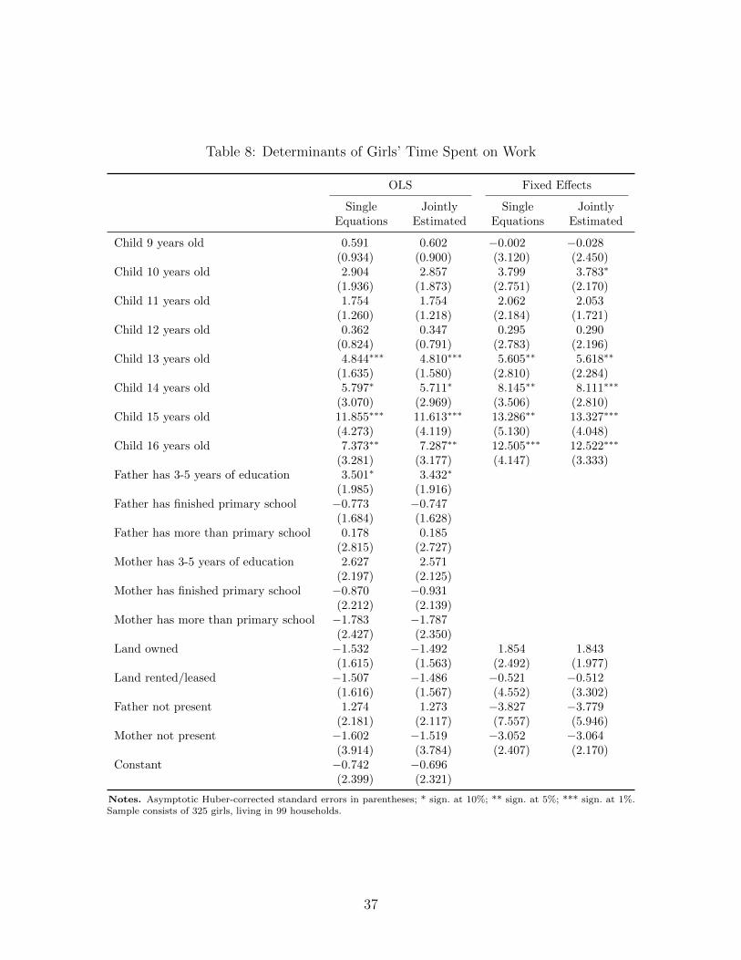
Table 8: Determinants of Girls’ Time Spent on Work
OLS Fixed Effects
Single Jointly Single JointlyEquations Estimated Equations Estimated
Child 9 years old 0.591 0.602 −0.002 −0.028(0.934) (0.900) (3.120) (2.450)
Child 10 years old 2.904 2.857 3.799 3.783∗
(1.936) (1.873) (2.751) (2.170)Child 11 years old 1.754 1.754 2.062 2.053
(1.260) (1.218) (2.184) (1.721)Child 12 years old 0.362 0.347 0.295 0.290
(0.824) (0.791) (2.783) (2.196)Child 13 years old 4.844∗∗∗ 4.810∗∗∗ 5.605∗∗ 5.618∗∗
(1.635) (1.580) (2.810) (2.284)Child 14 years old 5.797∗ 5.711∗ 8.145∗∗ 8.111∗∗∗
(3.070) (2.969) (3.506) (2.810)Child 15 years old 11.855∗∗∗ 11.613∗∗∗ 13.286∗∗ 13.327∗∗∗
(4.273) (4.119) (5.130) (4.048)Child 16 years old 7.373∗∗ 7.287∗∗ 12.505∗∗∗ 12.522∗∗∗
(3.281) (3.177) (4.147) (3.333)Father has 3-5 years of education 3.501∗ 3.432∗
(1.985) (1.916)Father has finished primary school −0.773 −0.747
(1.684) (1.628)Father has more than primary school 0.178 0.185
(2.815) (2.727)Mother has 3-5 years of education 2.627 2.571
(2.197) (2.125)Mother has finished primary school −0.870 −0.931
(2.212) (2.139)Mother has more than primary school −1.783 −1.787
(2.427) (2.350)Land owned −1.532 −1.492 1.854 1.843
(1.615) (1.563) (2.492) (1.977)Land rented/leased −1.507 −1.486 −0.521 −0.512
(1.616) (1.567) (4.552) (3.302)Father not present 1.274 1.273 −3.827 −3.779
(2.181) (2.117) (7.557) (5.946)Mother not present −1.602 −1.519 −3.052 −3.064
(3.914) (3.784) (2.407) (2.170)Constant −0.742 −0.696
(2.399) (2.321)
Notes. Asymptotic Huber-corrected standard errors in parentheses; * sign. at 10%; ** sign. at 5%; *** sign. at 1%.Sample consists of 325 girls, living in 99 households.
37

Table 9: Determinants of Girls’ Time Spent on Schooling
OLS Fixed Effects
Single Jointly Single JointlyEquations Estimated Equations Estimated
Child 9 years old 10.446∗∗∗ 10.442∗∗∗ 5.706 5.750∗
(3.863) (3.748) (4.533) (3.320)Child 10 years old 7.677∗∗ 7.694∗∗ 9.069∗ 9.072∗∗∗
(3.717) (3.606) (4.701) (3.490)Child 11 years old 16.142∗∗∗ 16.146∗∗∗ 13.285∗∗∗ 13.274∗∗∗
(3.526) (3.421) (3.739) (2.572)Child 12 years old 14.535∗∗∗ 14.540∗∗∗ 11.223∗∗∗ 11.219∗∗∗
(3.725) (3.614) (3.788) (2.594)Child 13 years old 6.520 6.539 5.948 5.953∗
(4.452) (4.319) (4.437) (3.162)Child 14 years old 5.143 5.183 4.343 4.335
(4.366) (4.235) (4.776) (3.357)Child 15 years old 5.641 5.728 2.628 2.613
(5.008) (4.859) (5.213) (3.607)Child 16 years old 8.686∗ 8.732∗ 6.309 6.272
(5.044) (4.893) (5.546) (3.823)Father has 3-5 years of education −0.204 −0.182
(3.129) (3.036)Father has finished primary school 8.329∗∗ 8.316∗∗∗
(3.280) (3.182)Father has more than primary school −0.865 −0.873
(4.354) (4.223)Mother has 3-5 years of education −5.263 −5.255
(3.426) (3.323)Mother has finished primary school 3.609 3.624
(3.913) (3.795)Mother has more than primary school 4.026 4.020
(4.242) (4.112)Land owned 4.424 4.411 −0.149 −0.139
(3.639) (3.531) (6.152) (4.101)Land rented/leased 1.124 1.106 −9.274 −9.254∗∗
(2.404) (2.332) (7.417) (3.659)Father not present −0.957 −0.942 −6.019 −6.081
(3.796) (3.684) (6.722) (4.507)Mother not present −8.236 −8.265 −25.169∗∗∗ −25.201∗∗∗
(5.908) (5.733) (8.898) (7.132)Constant 22.185∗∗∗ 22.181∗∗∗
(4.776) (4.633)
Notes. Asymptotic Huber-corrected standard errors in parentheses; * sign. at 10%; ** sign. at 5%; *** sign. at 1%.Sample consists of 325 girls, living in 99 households.
38

Table 10: Determinants of Girls’ Time Spent on Domestic Work
OLS Fixed Effects
Single Jointly Single JointlyEquations Estimated Equations Estimated
Child 9 years old 0.201 0.196 2.140 2.150(2.692) (2.612) (2.926) (2.321)
Child 10 years old 1.191 1.188 4.861 4.863∗
(2.493) (2.418) (3.232) (2.544)Child 11 years old 4.932∗∗ 4.927∗∗ 8.059∗∗∗ 8.061∗∗∗
(2.428) (2.356) (2.573) (1.990)Child 12 years old 4.862∗ 4.862∗∗ 7.898∗∗∗ 7.897∗∗∗
(2.530) (2.455) (2.945) (2.341)Child 13 years old 12.622∗∗∗ 12.626∗∗∗ 14.098∗∗∗ 14.081∗∗∗
(3.423) (3.321) (3.417) (2.739)Child 14 years old 11.299∗∗∗ 11.315∗∗∗ 15.600∗∗∗ 15.606∗∗∗
(3.116) (3.022) (3.107) (2.474)Child 15 years old 16.107∗∗∗ 16.146∗∗∗ 18.796∗∗∗ 18.763∗∗∗
(3.728) (3.620) (4.525) (3.535)Child 16 years old 8.474∗∗∗ 8.493∗∗∗ 11.481∗∗∗ 11.472∗∗∗
(2.848) (2.763) (3.486) (2.768)Father has 3-5 years of education −1.904 −1.899
(2.699) (2.617)Father has finished primary school −0.384 −0.389
(2.724) (2.642)Father has more than primary school 1.021 1.018
(3.135) (3.041)Mother has 3-5 years of education 3.995 4.012
(2.588) (2.512)Mother has finished primary school 2.463 2.473
(2.759) (2.678)Mother has more than primary school −2.967 −2.965
(2.829) (2.745)Land owned −1.326 −1.332 −2.645 −2.628
(1.829) (1.775) (4.422) (3.383)Land rented/leased −0.176 −0.182 −5.115 −5.122
(1.551) (1.505) (5.877) (4.222)Father not present −4.756∗∗∗ −4.755∗∗∗ −2.681 −2.692
(1.743) (1.691) (3.964) (2.878)Mother not present 7.339∗ 7.312∗ −2.061 −2.078
(4.411) (4.279) (3.506) (2.819)Constant 3.687 3.682
(3.490) (3.386)
Notes. Asymptotic Huber-corrected standard errors in parentheses; * sign. at 10%; ** sign. at 5%; *** sign. at 1%.Sample consists of 325 girls, living in 99 households.
39

Table 11: Correlation of Residuals and Fixed Effects be-tween Time Uses
OLS Fixed Effects
Jointly JointlyEstimated Estimated
BoysCorrelation of Individual Residuals
ρ(Work,School) −0.319∗∗∗ −0.304∗∗∗
(0.049) (0.053)ρ(Work,Domestic work) −0.085∗ −0.221∗∗∗
(0.044) (0.063)ρ(School,Domestic work) −0.119∗∗ −0.106∗
(0.060) (0.056)
Correlation of Household Fixed Effectsρ(Work,School) −0.279∗∗
(0.003)ρ(Work,Domestic work) 0.149
(0.114)ρ(School,Domestic work) −0.117
(0.215)
GirlsCorrelation of Individual Residuals
ρ(Work,School) −0.310∗∗∗ −0.177∗∗∗
(0.051) (0.057)ρ(Work,Domestic work) −0.091 −0.180∗∗∗
(0.057) (0.064)ρ(School,Domestic work) −0.166∗∗∗ −0.219∗∗∗
(0.060) (0.055)
Correlation of Household Fixed Effectsρ(Work,School) −0.420∗∗∗
(0.000)ρ(Work,Domestic work) 0.116
(0.254)ρ(School,Domestic work) −0.021
(0.839)
Notes. Asymptotic Huber-corrected standard errors in parentheses; * sign. at10%; ** sign. at 5%; *** sign. at 1%. Samples consist of 370 boys, living in 114households, and 325 girls, living in 99 households.
40