e cient walking speed optimization of a humanoid robot

Preprint of a manuscript submitted to:International Journal of Robotics Research

Efficient walking speed optimization of a

humanoid robot

T. Hemker∗, H. Sakamoto†, M. Stelzer∗, O. von Stryk∗

∗Technische Universitat Darmstadt,

Department of Computer Science,

Hochschulstraße 10, 64289 Darmstadt, Germany

hemker, stelzer, [email protected]

†Hajime Research Institute, Ltd., 5-6-21 Higashi Nakajima

Higashi Yodogawa-ku, Osaka 533-0033, Japan

[email protected]

1


Abstract

The development of optimized motions of humanoid robots that guar-

antee a fast and also stable walking is an important task especially in the

context of autonomous soccer playing robots in RoboCup. We present a

walking motion optimization approach for the humanoid robot prototype

HR18 which is equipped with a low dimensional parameterized walking

trajectory generator, joint motor controller and an internal stabilization.

The robot is included as hardware-in-the-loop to define a low dimensional

black-box optimization problem.

In contrast to previously performed walking optimization approaches

we apply a sequential surrogate optimization approach using stochas-

tic approximation of the underlying objective function and sequential

quadratic programming to search for a fast and stable walking motion.

This is done under the conditions that only a small number of physical

walking experiments should have to be carried out during the online op-

timization process. For the identified walking motion for the considered

55 cm tall humanoid robot we measured a forward walking speed of more

than 30 cm/s. With a modified version of the robot even more than 40

cm/s could be achieved in permanent operation.

2


1 Introduction

The speed of dynamically walking humanoid robots is a critical factor in many

applications, especially in autonomous robot soccer games. In this paper we

describe the successful approach undertaken for obtaining the fastest walking

humanoid robot in the autonomous humanoid robot league of RoboCup 2006.

Walking humanoid robots are high dimensional nonlinear dynamic multi-

body systems (MBS) with changing contact situations (impacts) and an under-

lying control of the joint motors. Many different approaches have already been

investigated for improving the walking speed of bipedal and quadrupedal robots.

However, all model-based optimization approaches have in common that their

outcome critically depends on the quality and accuracy of the robot model.

The derivation of highly accurate enough robot models to achieve the best pos-

sible walking speed may require too many efforts considering, e.g., the effects of

gear backlash, elasticity and temperature dependent joint friction or of different

ground properties. With a reasonable effort a MBS dynamics simulation of a

humanoid robot can only achieve an error of about 5 to 10 % compared to the

real system. Also a lot of additional work has to be spent in the transformation

of results from the simulated model to the real system before they can be used.

Furthermore, robot prototypes with the identical technical design differ sig-

nificantly in their motion even if the same motion control software is used. This

is due to inevitably small differences in the many robot components. For this

reason, the final improvement can only be obtained by working on the real robot.

An alternative approach to the optimization of walking motions based on de-

3


tailed MBS dynamics simulations is to start with a reasonable, initial walking

motion and then to use online hardware-in-the-loop optimization of the physical

robot prototype.

In our approach, a surrogate optimization methods is applied, that is based

on recent developments in the field. From our experience, this approach for

online optimization of the walking speed is much more efficient in terms of

function evaluations, i.e. walking experiments, required than random search

methods like genetic or evolutionary algorithms. The latter are usually applied

to cope with the robust minimization of noisy objective functions.

The paper is organized as follows. The following section gives a brief overview

on the problem to find stable walking motion for walking robots in general and

on the approaches to find fast and more robust motions. The third section de-

scribes the hardware and software components of the robot HR18 for which the

walking optimization is done. The fourth section points out the optimization

problem by objective function, variable domain, and gives a short overview on

optimization methods that are applicable for the arising kind of problem. The

here applied surrogate optimization method is introduced in the fifth section,

the sixth section describes the experimental setup and the result obtained from

the online optimization. The paper concludes by summarizing the main results.

4


2 Humanoid locomotion

2.1 Humanoid robots

The legs of all current humanoid robots which are able to reliably perform a

variety of different walking motions in experiments (as Honda ASIMO, HRP-2,

Johnnie or Sony QRIO) consist of rigid kinematic chains with 6 or 7 revolute

joints using electrical motors of high performance and with rigid gears for rotary

joint actuation. Only few initial approaches exist to insert and exploit elasticities

in humanoid robot locomotion, e.g. (Seyfarth et al., 2006). Commonly servo

motors are used in low- and medium-cost humanoid robots. However, there exist

specialized joint motors, gears and controllers designed for high-cost humanoid

robots (e.g. ASIMO, QRIO). A large variety of humanoid robots is involved in

the Humanoid Robot League of the RoboCup competitions (www.robocup.org).

Walking of humanoid robots is much more difficult than with four-legged

robots because during walking there must be phases where only one foot (or

even no foot at all) is in contact with ground. Therefore stability control is

much more an issue than with four-legged robots. Sensors are needed to detect

instabilities in a very early phase. Sophisticated software must evaluate the

sensors and modify the motion if needed to guarantee stability.

2.2 Walking optimization

Walking optimization generally may be done in two different ways: on compu-

tational models or on the real robot. Optimization on computational models

5


using optimal control techniques, e.g. (Denk and Schmidt, 2001; Buss et al.,

2003; Stelzer et al., 2003; Hardt and von Stryk, 2003), for both four-legged

and humanoid robots needs careful adaption of the model to the real robot and

successive refinements of the model so that the computed trajectories may be

implemented to the real robot. The iterations of the optimization procedure

however can be done without human assistance. Stability criteria may be used

in the optimization; therefore, methods that proved to be useful for four-legged

robots may be used for humanoid robots as well.

When optimization is done on the real robot, methods used for four and more

legged robots may not directly be used for humanoid robot as instabilities may

lead to severe damage of the robot. E.g. if the robot repeatedly falls down during

automated walking experiments for optimization. But promising results for a

hardware-in-the-loop optimization were e.g., presented in (Weingarten et al.,

2004), where a Nelder-Mead approach is applied successfully to improve the

walking speed of a six-legged robot.

Therefore, special approaches must be chosen. For four-legged robots, ap-

proaches based on parameterization of the walking motion and optimization of

the parameters by evaluation of the walking speed have been used successfully

(Kohl and Stone, 2004; Roefer, 2005). For biped robots, stability is much more

critical than for four-legged robots. (Behnke, 2006) suggested to let the hu-

manoid robot walk on a speed ramp during walking optimization as long as it is

stable and to measure stability implicitly by the distance the robot has covered

without falling down. Thus, an explicit modeling of walking stability for the

6


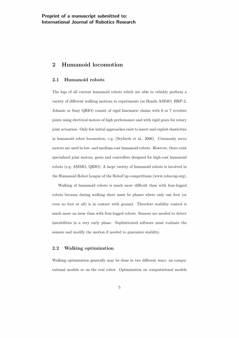
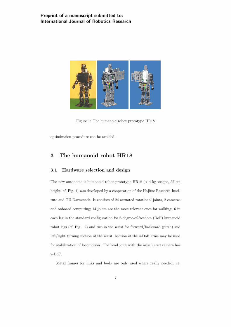
Figure 1: The humanoid robot prototype HR18

optimization procedure can be avoided.

3 The humanoid robot HR18

3.1 Hardware selection and design

The new autonomous humanoid robot prototype HR18 (< 4 kg weight, 55 cm

height, cf. Fig. 1) was developed by a cooperation of the Hajime Research Insti-

tute and TU Darmstadt. It consists of 24 actuated rotational joints, 2 cameras

and onboard computing; 14 joints are the most relevant ones for walking: 6 in

each leg in the standard configuration for 6-degree-of-freedom (DoF) humanoid

robot legs (cf. Fig. 2) and two in the waist for forward/backward (pitch) and

left/right turning motion of the waist. Motion of the 4-DoF arms may be used

for stabilization of locomotion. The head joint with the articulated camera has

2-DoF.

Metal frames for links and body are only used where really needed, i.e.

7


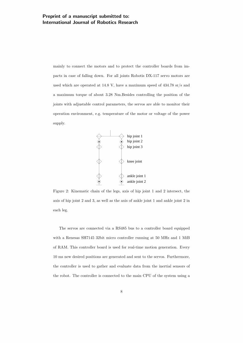
mainly to connect the motors and to protect the controller boards from im-

pacts in case of falling down. For all joints Robotis DX-117 servo motors are

used which are operated at 14.8 V, have a maximum speed of 434.78 sr/s and

a maximum torque of about 3.28 Nm.Besides controlling the position of the

joints with adjustable control parameters, the servos are able to monitor their

operation environment, e.g. temperature of the motor or voltage of the power

supply.

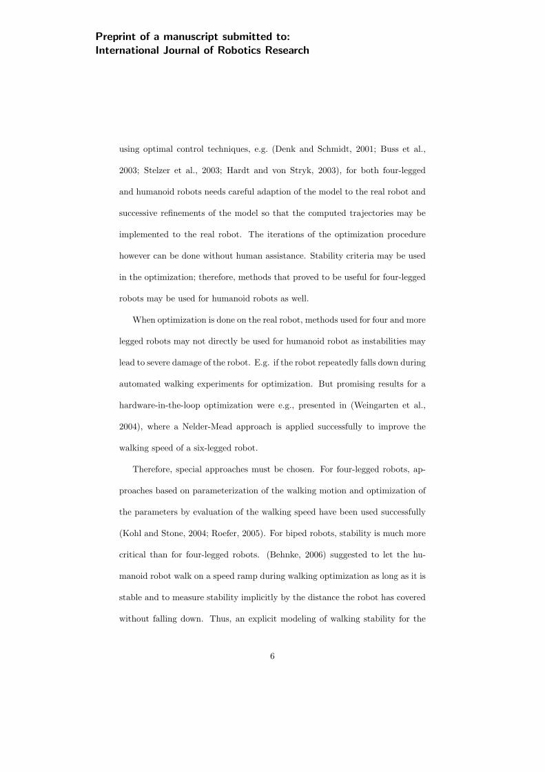
hip joint 1hip joint 2

hip joint 3

knee joint

ankle joint 1

ankle joint 2

Figure 2: Kinematic chain of the legs, axis of hip joint 1 and 2 intersect, the

axis of hip joint 2 and 3, as well as the axis of ankle joint 1 and ankle joint 2 in

each leg.

The servos are connected via a RS485 bus to a controller board equipped

with a Renesas SH7145 32bit micro controller running at 50 MHz and 1 MiB

of RAM. This controller board is used for real-time motion generation. Every

10 ms new desired positions are generated and sent to the servos. Furthermore,

the controller is used to gather and evaluate data from the inertial sensors of

the robot. The controller is connected to the main CPU of the system using a

8


RS232 connection running at 57.6 KiB/s.

Lithium polymer rechargeable battery packages are used for onboard power

supply because of their good ratio between mass and capacity, a 4-cell 14.8 V

battery for actuation of the motors, and a 2-cell battery for the controller board.

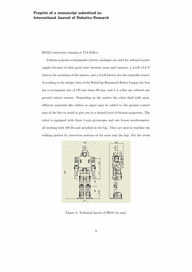
According to the design rules of the RoboCup Humanoid Robot League the foot

has a rectangular size of 125 mm times 90 mm, and it is a flat one without any

ground contact sensors. Depending on the surface the robot shall walk upon,

different materials like rubber or paper may be added to the ground contact

area of the feet to avoid or give rise to a desired level of friction properties. The

robot is equipped with three 1-axis gyroscopes and one 3-axes accelerometer,

all working with 100 Hz and attached in the hip. They are used to stabilize the

walking motion by correction motions of the arms and the legs. For the needs

Figure 3: Technical layout of HR18 (in mm)

9


of acting in a highly dynamically environment like it is arising for autonomous

soccer games in RoboCup, the HR18 has been equipped at TU Darmstadt with

two off-the-shelf webcams and a pocket PC to enable autonomous soccer playing.

3.2 High- and low-level software

Two levels of software are used on the robot. On a pocket PC the high-level

software is running. It consists of a framework (Friedmann et al., 2006b) that co-

ordinates the control architecture with sensor data processing, self localization,

world modeling, hierarchical finite state machine for behavior control (Lotzsch

et al., 2006), and finally the motion generation/requests. The motion requests

are sent via the described serial port to the controller board.

The low-level software on this board distinguishes between two different

kinds of motions: Walking motions and so called special motions. The first ones

are parameterized by certain parameters (cf. Section 3.3), and the latter ones

are teach-in-motions that are stored by joint angle trajectories. All motions are

PD-controlled on joint angle level by the servo-motors.

The inertial sensor values are used to reduce vibration of unbalance during

walking or other motions with a PD controller. The vibration is caused by a

fast, but simplified calculation of the zero moment point (ZMP) or by uneven

terrain. The PD control is useful to stabilize especially during the fast walking

of the robot. It is calculated by

θnew = θ +Kp ∗ ωgyro +Kd ∗d

dtωgyro

for the joint motors of the foot pitch, the foot roll, the hip pitch, the hip roll, the

10


waist pitch, the shoulder pitch, and finally the shoulder roll, herein described as

θ for the angle calculated by inverse kinematics and θnew the controlled angle;

Kp and Kd are the PD control parameter and ωgyro is the angular velocity of

the gyro. The values for Kp and Kd are identified by expert knowledge and

experiments.

Direct access to the memory of the robot exists, i.e. all parameters may

be changed during run time which allows easy alteration of walking or sensory

parameters and debugging.

3.3 Parameterization of humanoid walking trajectories

Like any motion, walking motion may be described by joint angle trajectories.

These however are infinite dimensional and therefore hard to handle. In contrast

to special motions like shooting the ball, waving, getting down or standing

up, walking is a periodical and comparatively smooth motion. Therefore, the

y

2 y_ZMP

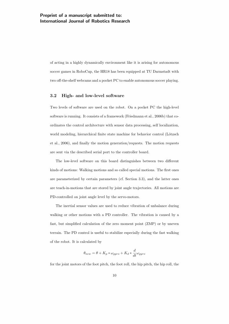
Figure 4: Footprint of the walking motion and desired ZMP position yZMP

walking motion may be generated by prescribing trajectories for the hip and

the feet and solving the inverse kinematics for the joint angles. The inverse

kinematics model can be calculated analytically due to the special kinematic

11


structure of the leg (Fig. 2). The trajectories for x-, y-, and z-position of feet

relatively given to the hip are parameterized by geometric parameters, which

leads depending on the number of time steps to a high dimensional (finite,

however) discretization of the walking motion. The three dimensional walking

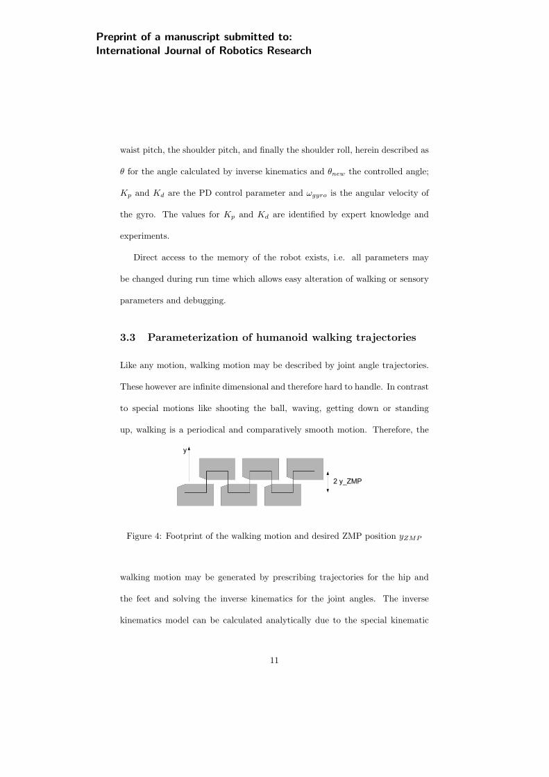
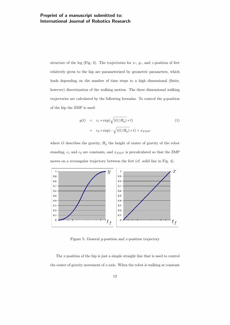
trajectories are calculated by the following formulas. To control the y-position

of the hip the ZMP is used:

y(t) = c1 ∗ exp(√

(G/Hg) ∗ t) (1)

+ c2 ∗ exp(−√

(G/Hg) ∗ t) + xZMP

where G describes the gravity, Hg the height of center of gravity of the robot

standing, c1 and c2 are constants, and xZMP is precalculated so that the ZMP

moves on a rectangular trajectory between the feet (cf. solid line in Fig. 4).

Figure 5: General y-position and x-position trajectory

The x-position of the hip is just a simple straight line that is used to control

the center of gravity movement of x-axis. When the robot is walking at constant

12


speed, the ZMP of the x-axis is 0 and is neglected. The curves describing the

z-position, the distance between hip and foot, and described by two curves, one

for lifting (zup) and a second for dropping (zdw). Both are moving fast close

to the ground to reduce the influence of the ground error and to reduce inertia

during swing of the leg. For lifting and dropping the foot we use

zup(t) =zheight·c4

π

(π

2− arcsin

(1− t

tf

)− c3

), (2)

respectively

zdw(t) = zup(1− t), (3)

as basis functions, with zheight as maximum desired height in z direction of the

foot and tf as final time of one step.

Figure 6: General z-position trajectory

Finally parameter tuning by hand identified particularly the most important

parameters summarized by p for stable walking. Those are the relation of the

13


distances of the front and of the rear leg to the center of mass, the lateral

position, the roll angle and the height above ground of the foot during the

swing phase, and the pitch of the upper body.

By aggregating the curves for a walking motion and scaled by p we obtain

completely parameterized three dimensional walking motion trajectories. And

these parameters scale and shift the defined walking trajectories in Equations (1)

to (3) during the optimization process, where the other parameters are assumed

to be constant with suitable values which are determined by expert knowledge

and experiments.

Using finally the symmetry of the walking motions the parameter for the

lateral position of the right foot can be set to the negative lateral position of

the left foot during the swinging phase, just as well as the roll angle of the right

foot has to be the negativ roll angle of the left foot. With this procedure we

obtain a six dimensional parameterization of a forward walking trajectories at

a fixed step frequency.

4 The optimization problem

4.1 Modeling of the objective function

As quality or objective function value for a parameter set defining a walking

motion we measure the distance the robot covers on the experimental field until

it stops or falls. It starts with a small step length 110 mm and the step length is

increased every 2 steps by 5 mm, so that the final step length of 240 mm would

14


be reached after 52 steps, always with a constant frequency of about 2.85 steps

per second. It follows that the walking speed is only influenced directly by the

applied step length.

This definition of the objective function includes constraints for maintaining

walking stability of the walking motion implicitly, which otherwise would have to

be formulated analytically with a high effort to incorporate them explicitly into

the definition of the here considered optimization problem. Only robust walking

motions for all step lengths between 110 mm and 240 mm have a chance to reach

a high objective function value, because during the measurement 27 different

step lengths are applied. This ensure that a found walking motion is a fast but

also robust one for different velocities.

4.2 Feasible domain of optimization variables

The above introduced number of relevant parameters for the walking motion is

reduced with this objective function definition by another dimension to finally

five optimization variables. The variation of the step length during the walk-

ing experiment, the x-position of one foot in front of the upper body and the

x-position of the other foot behind the upper body during a step are reduced

to only one variable. This variable describes the proportion between both. For

all applied values for the step length, both parameters are described uniquely.

During the online optimization the five real-valued variables that are influencing

the main characteristics of the walking behavior of the robot are being varied

to maximize the defined objective function only regarding to box constraints.

15


These bounds for the optimization parameters must be strictly met by the opti-

mization method for each trial walk of the robot occurring during one evaluation

of the objective function. The bounds are set to values for which a wide range

of variations of the walking motion is possible. But the bounds also guarantee

that no contacts of moving parts of the robot can occur.

4.3 Classification of the optimization problem

The robot is included as hardware in the loop for the walking experiment to

evaluate the objective function f measuring the walking speed. In this context

a non deterministic black-box optimization problem with box constraints arises,

where besides a noisy function value of f no further information is provided. Es-

pecially no gradient information can be provided which would be compulsive for

effective gradient based optimization. Even the approximation of gradients by

finite differences is not applicable because of the non deterministic experimental

results. Additionally we are also not able to proof properties like continuity or

differentiability of the objective function because of the black box characteristic

of the problem. The resulting mathematical formulation of the optimization

problems reads as follows:

maxp∈Ω

f(p), f : IR5 → IR,

with

Ω = p ∈ IR5|p(l) ≤ p ≤ p(u), p(l),p(u) ∈ IR5.

16


This leads to the question which optimization methods can be applied to find a

good walking motion with reasonable efforts.

4.4 Optimization methods

The arising optimization problem impedes the direct use of any kind of superlin-

ear or quadratically convergent gradient based or Newton type methods because

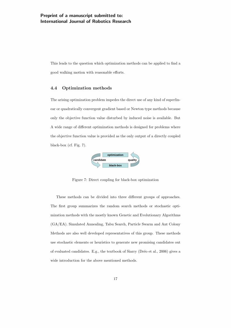
only the objective function value disturbed by induced noise is available. But

A wide range of different optimization methods is designed for problems where

the objective function value is provided as the only output of a directly coupled

black-box (cf. Fig. 7).

black-box

optimization

candidate quality

Figure 7: Direct coupling for black-box optimization

These methods can be divided into three different groups of approaches.

The first group summarizes the random search methods or stochastic opti-

mization methods with the mostly known Genetic and Evolutionary Algorithms

(GA/EA). Simulated Annealing, Tabu Search, Particle Swarm and Ant Colony

Methods are also well developed representatives of this group. These methods

use stochastic elements or heuristics to generate new promising candidates out

of evaluated candidates. E.g., the textbook of Siarry (Dreo et al., 2006) gives a

wide introduction for the above mentioned methods.

17


The second group consists of sampling methods. These are on the one hand

side direct optimization methods (Lewis et al., 2000) like the Pattern Search

(Griffin and Kolda, 2006; Torczon, 1997), or DIRECT (Jones et al., 1998) which

only include the information if improvement is obtained or not. On the other

side we have sampling methods that include the objective function values also

as quantitative information. These are, e.g., the Nelder-Mead simplex approach

(Nelder and Mead, 1965), extension of this idea, or implicit filtering (Choi et al.,

1999; Kelley, 2005) as a projected Quasi-Newton Method. Another way to

subdivide the group of sampling methods is the characteristic, if the search is

grid-based (e.g. pattern search) or not (e.g., Nelder-Mead), or if it is stencil

based (e.g., implicit filtering) or not (e.g., DIRECT). But all sampling methods

have in common that new candidates are generated during their search for a

maximum/minimum by exploring promising areas, or using bigger steps to find

promising areas of the search domain.

Both groups of methods are often applied to simulation based optimization

problems, which do not differ too much from the here considered walking opti-

mization problem. With the main weight on the number of function evaluation

a method needs, it has been shown that sampling methods can outperform ran-

dom search methods on well modeled problems (Fowler et al., 2004), but are

not as easy to apply as the often very user friendly implemented GAs or EAs.

In our case each function evaluation needs a physical experiment, which means

use and wear of the robot, manpower for observing, and expensive lab time.

The third group of methods are the surrogate optimization methods. Here,

18


the optimization is not performed directly on the objective function but on a ap-

proximation of it as described, e.g., in (Sacks et al., 1989; Jones et al., 1998) or

(Alexandrov, 2001). In (Hemker et al., 2006a) and (Hemker et al., 2006b) such

a method based on sequential stochastic approximations in combination with

sequential quadratic programming was successful applied to simulation based

black-box problems with expensive function evaluations. This optimization ap-

proach easily can incorporate very general, linear and nonlinear, equality or

inequality constraints on the optimization parameter values, not only box con-

straints. This is another huge advantage compared to the two other groups of

methods. Because of the efficiency shown for these applications regarding to the

needed objective function evaluations, the therein proposed method is adapted

to the humanoid robot walking optimization problem and is described in the

next section.

5 Sequential surrogate optimization

5.1 Design and analysis of computer experiments

The optimization method we apply consists in each iteration of a statistical ap-

proximation method that calculates a smooth surrogate function of the original

objective function. Many different methods exist and are used in the context

of surrogate optimization. As a standard approach designed for deterministic

black-box optimization problems, design and analysis of computer experiments

(DACE) described by Sacks et al. (Sacks et al., 1989) is widely used, which has

19


its origins in the geostatistical kriging method (Matheron, 1963). But even for

non-deterministic functions this method is able to catch the main characteristics

if the deviation is in comparison to the mean not too high to mask the main

properties of the considered objective function f .

A DACE model f is in it’s general form a two component model,

f(p) =k∑

j=1

βjhj(p) + Z(p).

The first and more global part approximates the global trend of the unknown

function f by a linear combination of a scalar vector β ∈ IRk and k known fixed

functions hj . Different approaches can be considered for this first part (Martin

and Simpson, 2003). Universal kriging is predicting the mean of the underlying

function as a realization of a stochastic process by a linear combination of k

known basis functions on the whole domain, as well as detrended kriging applies

a classical linear regression model. In our application we follow the idea of

ordinary kriging where a constant mean is assumed on the whole domain with

k = 1 and one constant h.

The second part Z guarantees that the DACE model f fits to f for a number

of sets of points p(i), i = 1, ..., n, out of the variable space,

f(p(i)) = f(p(i)), i = 1, ..., n.

This part is assumed to be a realization of a stationary Gaussian random func-

tion with a mean of zero, E[Z(p)] = 0, and a covariance

Cov[Z(p(i)), Z(p(j))] = σ2R(p(i),p(j)),

20


with i 6= j, and i, j ∈ 1, ..., n. The smoothness and properties like differen-

tiability are controlled by the chosen correlation function R, in our case the

product of one dimensional correlation functions Rj ,

R(p(1),p(2)) =

np∏

j=1

Rj(|p(1)j − p

(2)j |),

and the Gaussian correlation function,

Rj(|p(1)j − p

(2)j |) = exp(−θ|p(1)

j − p(2)j |q),

with q = 2, as a special case of the generalized exponential correlation function

with 0 < q < 2 and θ ∈ (0,∞) proposed by Sacks et al. (Sacks et al., 1989).

By maximum likelihood estimation the process variance σ2, the regression pa-

rameter β, and the correlation parameter θ used to define R are estimated most

consistent to the present objective function values to which f has to fit. As ad-

ditional information we can evaluate the expected mean square error (MSE) of

the actual model. Under the assumption that the approximated function really

behaves like a Gaussian random process, the MSE of the DACE model gives an

estimation of the approximation quality for a certain p. This is needed later

during the sequential update procedure. For a more detailed description on the

theory behind these kind of models we refer the reader to (Koehler and Owen,

1996).

5.2 Sequential update process

We start the optimization process with an experiment, where an initial point

p for approximation of the first surrogate function is chosen by prior obtained

21


expert knowledge to provide a stable but possibly slow, initial humanoid robot

walking motion. An initial set of experiments is generated around the initial

motion by varying each single variable dimension pi on its own by 10 % of

the total range of the feasible domain, like it is known from other optimization

methods by sampling (Griffin and Kolda, 2006). In our case this leads to eleven

sampled points for which the objective function value is known. With this

knowledge the first surrogate function f1 is built. With this first surrogate

function the initial phase of this optimization procedure is finished and the

main iteration starts. This analytically given surrogate is maximized regarding

to the defined box constraints on p.

The maximum of the surrogate function f is added to the set of basis points

for the DACE model in the next iteration step. Such sequential procedures

are discussed in more detail in (Sasena, 2002). However, in contrast to the

update strategies discussed therein, we use convergence to a previously deter-

mined parameter set as criteria to stop maximizing f and to search for a new

candidate parameter set. If the distance of a found maximum to a point already

evaluated by experiments falls below a defined limit, not the actual maximum,

but the maximum of the MSE of the surrogate function is searched, evaluated,

and added to the set of basis points for approximation. The MSE of a DACE

model can be calculated easily if the model itself is determined as described

in (Sacks et al., 1989). This procedure improves the approximation quality of

the surrogate function in unexplored regions of the parameter domain. The

objective function value for this new candidate is determined by performing the

22


corresponding walking experiment with the humanoid robot.

After a new point is added, a new surrogate function is generated with a

new DACE model and the optimization starts again. The sequential procedure

is summarized in a general setting in the following algorithm:

Algorithm 1 Sequential update for objective function f and variable p:1: Evaluate f(p(i)) for a set of basis points p(i), with i = 1, ..., N .

2: Build surrogate function f by running DACE with the set of basis points

p(i), for i = 1, ..., n.

3: Search the minimum p∗ of f .

4: If p∗ is too close to a basis point, |p∗−p(i)| ≤ ε, i = 1, ..., n, go to 5, else to

go 6.

5: Search for the maximum pMSE∗ of the MSE(f).

6: Add p∗ respectively pMSE∗ to the set of basis points, stop or go to step 1.

The key feature of surrogate optimization approaches is that the optimiza-

tion methods avoids from running directly in a loop with the real system that

generates the original optimization problem, but calls the surrogate problem

on which emerging computational costs to determine new promising points to

test with the real system system can be neglected if the costs of running a real

walking experiment are taken into account.

5.3 Implementation details

The complete optimization procedure is implemented in Matlab and uses two

additional standard toolboxes. The first one is the DACE toolbox (Lophaven

23


et al., 2002), that generates in each iteration the DACE model and is called

directly by the optimizer for the function values f(p) to find the maximum p∗

of f , respectively the maximum pMSE∗ of the MSE of f . The second component

is the optimizer SNOPT (Gill et al., 2006), a sophisticated implementation of

sequential quadratic programming (SQP).

The idee behind SQP methods as described in (Gill et al., 2005) is to solve

a nonlinear programming problem by using a sequence of quadratic subprob-

lems. It is a highly efficient optimization method for smooth analytically defined

nonlinear programming including also nonlinear constraints problems, even for

large scale problems with many optimization variables and constraints. In our

case only nonlinear programming problems of small scale are arising with simple

constant bounds on the variables, which have to be solved during each iteration

of the described sequential surrogate optimization approach.

6 Experimental and numerical results

6.1 Experimental setup and procedure

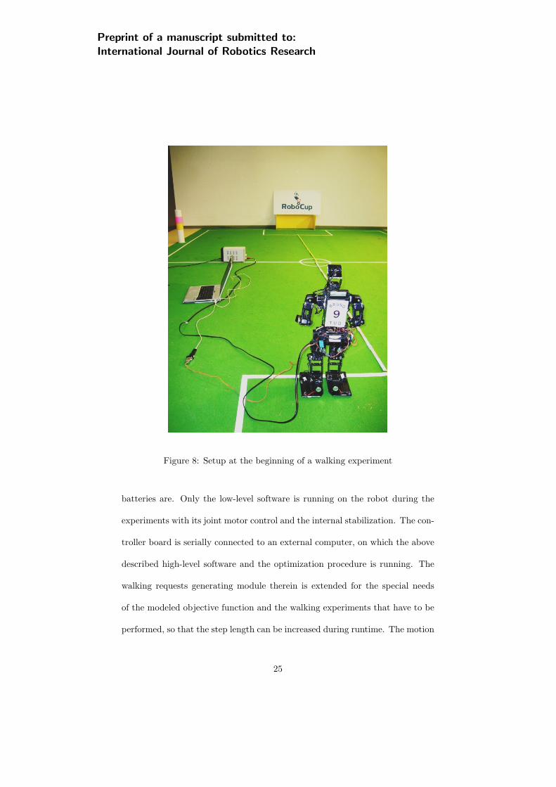
All walking experiments with the humanoid robot HR 18 are performed on a

standard RoboCup soccer field (cf. Fig. 8). To guarantee constant conditions

during the experiments the joint motors are supplied by a continuous external

power supply where the batteries are only used as weights to provide the op-

erating condition the robot meets in the intended soccer application. For the

walking experiments the Pocket PC is only carried for the same reason as the

24


Figure 8: Setup at the beginning of a walking experiment

batteries are. Only the low-level software is running on the robot during the

experiments with its joint motor control and the internal stabilization. The con-

troller board is serially connected to an external computer, on which the above

described high-level software and the optimization procedure is running. The

walking requests generating module therein is extended for the special needs

of the modeled objective function and the walking experiments that have to be

performed, so that the step length can be increased during runtime. The motion

25


generation obtains new walking parameter sets from the optimization procedure

as a text file and sends walking requests for walking experiments together with

the walking parameters to the robot.

Of course not every new parameter set that is generated by the optimization

procedure results in a walking motion where the robot is really walking forward

or is even able to walk one step without falling. For such parameter sets p we

assign zero as the objective function value. All walking experiments start at

the same position heading into the same direction. The distance covered by the

robot during walking is measured by visual inspection of the human operator

in an accuracy of about ±5 cm. In principle the covered distance can also be

measured by one of the onboard cameras using a standard geometrical object

with given shape, color, and constant position. Additionally the temperature

of the joint motors as a possible critical factor is observed manually during all

experiments, to guarantee no overheating at any time. The power cord, the

serial connection, and a belt to protect the robot from damage in the case that

it falls down are carried by a human helper, but it is keenly observed that the

robot’s motions are not influenced by the cables and the belt.

6.2 Numerical and experimental results

The initial parameter set p(ini) has been obtained earlier by tuning of the pa-

rameters by hand and the definition of p as described at the end of Section 3.3 is

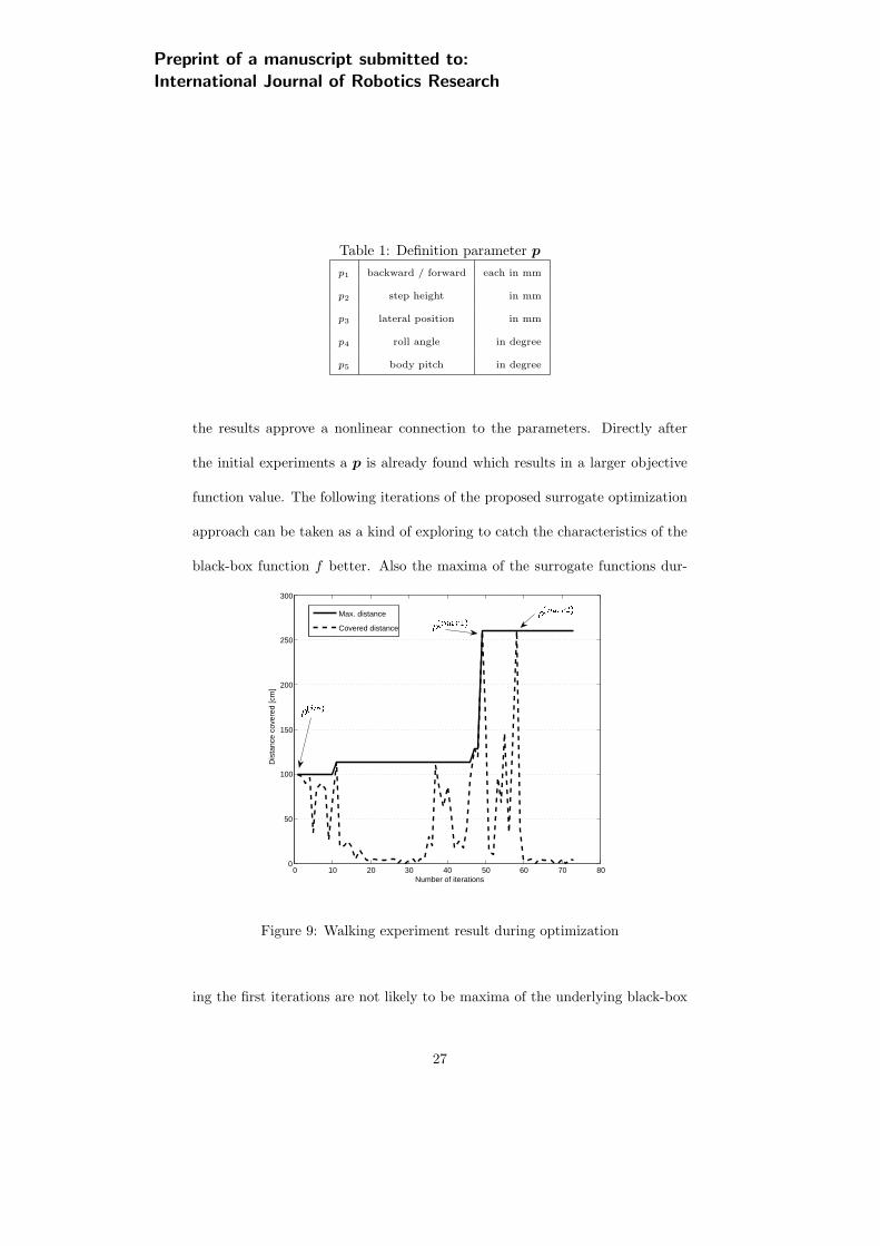
summarized in Table 1. As we can see from the objective function values (Fig. 9)

during the eleven initial walking experiments during the optimization process,

26


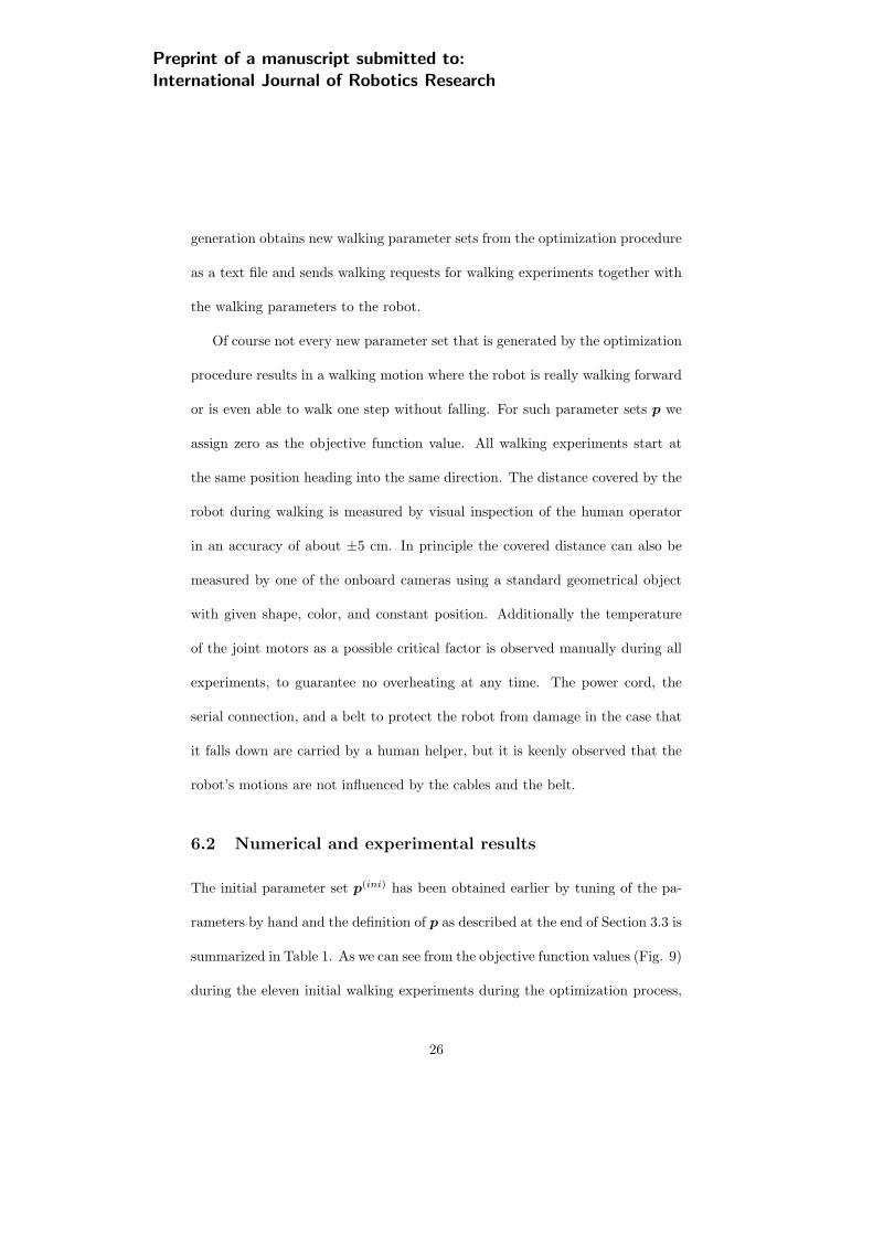
Table 1: Definition parameter p

p1 backward / forward each in mm

p2 step height in mm

p3 lateral position in mm

p4 roll angle in degree

p5 body pitch in degree

the results approve a nonlinear connection to the parameters. Directly after

the initial experiments a p is already found which results in a larger objective

function value. The following iterations of the proposed surrogate optimization

approach can be taken as a kind of exploring to catch the characteristics of the

black-box function f better. Also the maxima of the surrogate functions dur-

0 10 20 30 40 50 60 70 800

50

100

150

200

250

300

Number of iterations

Dis

tanc

e co

vere

d [c

m]

Max. distance

Covered distance

Figure 9: Walking experiment result during optimization

ing the first iterations are not likely to be maxima of the underlying black-box

27


function as can be observed from iteration 18 to 32 in Fig. 9. But by finding

promising areas, improvements in form of two candidates p(max1) and p(max2)

are identified, where the robot covers the same distance after performing all 52

steps of a walking experiment with stopping at the end without falling. Both

candidates are identified during maximizing the surrogate and not the MSE.

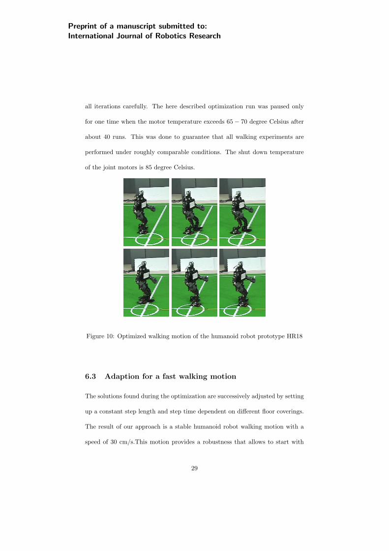
The motion resulting from the set p(max1) is visualized in Fig. 10. Even after

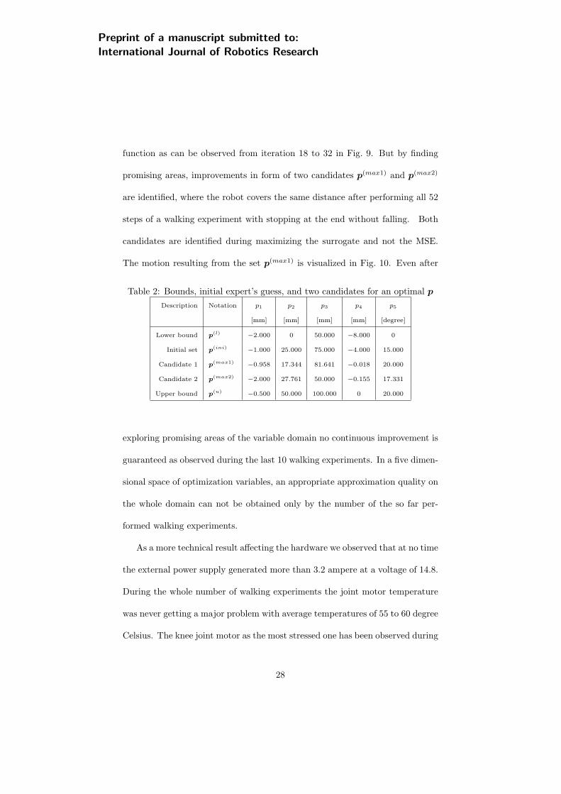
Table 2: Bounds, initial expert’s guess, and two candidates for an optimal p

Description Notation p1 p2 p3 p4 p5

[mm] [mm] [mm] [mm] [degree]

Lower bound p(l) −2.000 0 50.000 −8.000 0

Initial set p(ini) −1.000 25.000 75.000 −4.000 15.000

Candidate 1 p(max1) −0.958 17.344 81.641 −0.018 20.000

Candidate 2 p(max2) −2.000 27.761 50.000 −0.155 17.331

Upper bound p(u) −0.500 50.000 100.000 0 20.000

exploring promising areas of the variable domain no continuous improvement is

guaranteed as observed during the last 10 walking experiments. In a five dimen-

sional space of optimization variables, an appropriate approximation quality on

the whole domain can not be obtained only by the number of the so far per-

formed walking experiments.

As a more technical result affecting the hardware we observed that at no time

the external power supply generated more than 3.2 ampere at a voltage of 14.8.

During the whole number of walking experiments the joint motor temperature

was never getting a major problem with average temperatures of 55 to 60 degree

Celsius. The knee joint motor as the most stressed one has been observed during

28


all iterations carefully. The here described optimization run was paused only

for one time when the motor temperature exceeds 65− 70 degree Celsius after

about 40 runs. This was done to guarantee that all walking experiments are

performed under roughly comparable conditions. The shut down temperature

of the joint motors is 85 degree Celsius.

Figure 10: Optimized walking motion of the humanoid robot prototype HR18

6.3 Adaption for a fast walking motion

The solutions found during the optimization are successively adjusted by setting

up a constant step length and step time dependent on different floor coverings.

The result of our approach is a stable humanoid robot walking motion with a

speed of 30 cm/s.This motion provides a robustness that allows to start with

29


the found maximum speed and to perform an abrupt stop without unbalancing

the robot, even on different floor coverings.

All walking experiments during the optimization run have been performed

on a single in time slot of about four hours, including breaks of about one hour,

and less than 100 walking experiments including a warming up of the robot.

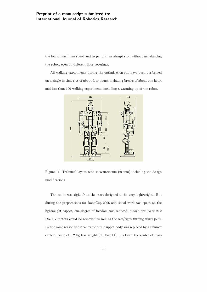
Figure 11: Technical layout with measurements (in mm) including the design

modifications

The robot was right from the start designed to be very lightweight. But

during the preparations for RoboCup 2006 additional work was spent on the

lightweight aspect, one degree of freedom was reduced in each arm so that 2

DX-117 motors could be removed as well as the left/right turning waist joint.

By the same reason the steal frame of the upper body was replaced by a slimmer

carbon frame of 0.2 kg less weight (cf. Fig. 11). To lower the center of mass

30


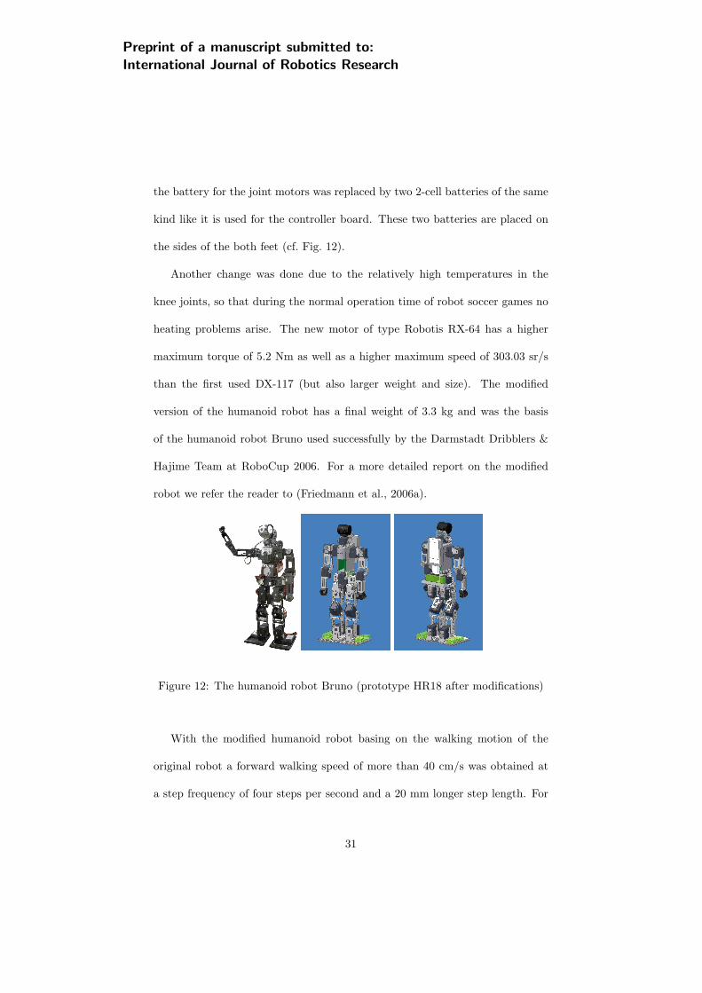
the battery for the joint motors was replaced by two 2-cell batteries of the same

kind like it is used for the controller board. These two batteries are placed on

the sides of the both feet (cf. Fig. 12).

Another change was done due to the relatively high temperatures in the

knee joints, so that during the normal operation time of robot soccer games no

heating problems arise. The new motor of type Robotis RX-64 has a higher

maximum torque of 5.2 Nm as well as a higher maximum speed of 303.03 sr/s

than the first used DX-117 (but also larger weight and size). The modified

version of the humanoid robot has a final weight of 3.3 kg and was the basis

of the humanoid robot Bruno used successfully by the Darmstadt Dribblers &

Hajime Team at RoboCup 2006. For a more detailed report on the modified

robot we refer the reader to (Friedmann et al., 2006a).

Figure 12: The humanoid robot Bruno (prototype HR18 after modifications)

With the modified humanoid robot basing on the walking motion of the

original robot a forward walking speed of more than 40 cm/s was obtained at

a step frequency of four steps per second and a 20 mm longer step length. For

31


the modified robot the walking motion needed some steps for acceleration with

increasing step-length because of the increased total step-length to get into a

stable walking motion of 40 cm/s, which is needed on the original robot. But

it also performs a stable instant stop in one step without falling down.

During RoboCup 2006 several demo footraces have been performed with

other humanoid robots and four-legged Sony AIBO robots where Bruno clearly

demonstrated to be the fastest humanoid robot. In a demo race, it also out-

performed the much taller finalists of the footrace competition of the TeenSize

humanoid robots taller than 65 cm.

7 Conclusion

For the newly developed, 55 cm tall autonomous humanoid robot prototype

HR18 a hardware-in-the-loop walking optimization approach has been presented.

The optimization problem formulation is based on a suitable parameterization

of the walking trajectories, where a small number of parameters are used as

optimization variables. During fast walking the underlying joint servo motor

control is stabilized using inertial sensing which is part of the low-level soft-

ware running on the robot’s controller board. Under this preconditions it was

demonstrated that efficient walking speed optimization can be obtained even

with a quite small number of functions evaluations. In only about 50 walking

experiments a 30 cm/s fast walking motion has been obtained using a sequential

surrogate optimization approach. In further experiments, it was observed that

32


as an interesting side effect the obtained walking motion is also robust in a sense

that the performance is also well does not change much on different floor cov-

erings which have not been used during the optimization. A further improved

hardware design of the robot prototype HR18 resulted in the prototype Bruno.

With a short starting phase for acceleration from stand still a further increase

of the forward walking speed to more than 40 cm/s was achieved. The de-

scribed optimization approach can be applied to other types of humanoid robot

locomotion like turning or walking sidewards as well.

Because the surrogate model is smooth and reflects the main characteristics

of the approximated noisy objective function it can be solved very efficiently

with superlinearly converging Newton-type methods. Thus only relatively few

walking experiments with the real robot are needed. Another advantage com-

pared with heuristic search methods as genetic or evolutionary algorithms is

that very general explicit constraints, as linear or nonlinear, inequality and

equality constraints, on the optimization variables can easily be included in the

optimization problem. Finally, it should be noted that the measurement of the

covered distance can as well be performed by the robot itself. With one of its

cameras the robot can with only little efforts compute the current distance to

an object with known geometrical shape, color, and position.

33


Acknowledgments

Parts of this research were supported by the German Research Foundation

(DFG) within the Research-Training-Group 853 “Modeling, Simulation, and

Optimization of Engineering Applications” and the Priority Program 1125 “Ko-

operierende Teams mobiler Roboter in dynamischer Umgebung”.

References

Alexandrov, N. M. (2001). An overview of first-order model management for

engineering optimization. Optimization and Engineering, 2:413430.

Behnke, S. (2006). personal communication.

Buss, M., Hardt, M., Kiener, J., Sobotka, J., Stelzer, M., von Stryk, O., and

Wollherr, D. (2003). Towards an autonomous, humanoid, and dynamically

walking robot: Modeling, optimal trajectory planning, hardware architec-

ture, and experiments. In Proc. IEEE/RAS Humanoids 2003. Springer-

Verlag.

Choi, T., Gilmore, P., Eslinger, O., Patrick, A., Kelley, C., and Gablonsky,

J. (1999). IFFCO: Implicit Filtering for Constrained Optimization, Ver-

sion 2. Technical Report CRSC-TR99-23, Center for Research in Scientific

Computation.

Denk, J. and Schmidt, G. (2001). Synthesis of a walking primitive database for a

humanoid robot using optimal control techniques. In Proceedings of IEEE-

34


RAS International Conference on Humanoid Robots (HUMANOIDS2001),

Tokyo, Japan, November 2001, pages 319–326.

Dreo, J., Siarry, P., Petrowski, A., and Taillard, E. (2006). Metaheuristics for

Hard Optimization. Springer.

Fowler, K., Kelley, C., Miller, C., Kees, C., Darwin, R., Reese, J., Farthing, M.,

and Reed, M. (2004). Solution of a well-field design problem with implicit

filtering. Optimzation and Engineering, 5:207–233.

Friedmann, M., Kiener, J., Petters, S., Sakamoto, H., Thomas, D., and von

Stryk, O. (2006a). Versatile, high-quality motions and behavior control of

humanoid soccer robots. In Proc. Workshop on Humanoid Soccer Robots

of the 2006 IEEE-RAS Int. Conf. on Humanoid Robots, pages 9–16.

Friedmann, M., Kiener, J., Petters, S., Thomas, D., and von Stryk, O. (2006b).

Reusable architecture and tools for teams of lightweight heterogeneous

robots. In Proc. 1st IFAC-Symposium on Multivehicle Systems, pages 51–

56, Salvador, Brazil.

Gill, P., Murray, W., and Saunders, M. (2005). SNOPT: An SQP algorithm for

large-scale constrained optimization. SIAM REVIEW, 47(1):99131.

Gill, P., Murray, W., and Saunders, M. (2006). User’s guide for SNOPT 7.1:

a fortran package for large-scale nonlinear programming. Report NA 05-2,

Department of Mathematics, University of California, San Diego.

Griffin, J. and Kolda, T. (2006). Asynchronous parallel generating set search

35


for linearly-constrained optimization. Technical report, Sandia National

Laboratories, Albuquerque, NM and Livermore, CA.

Hardt, M. and von Stryk, O. (2003). Dynamic modeling in the simulation, op-

timization and control of legged robots. In: ZAMM: Zeitschrift fur Ange-

wandte Mathematik und Mechanik, 83(10):648–662.

Hemker, T., Fowler, K., and von Stryk, O. (2006a). Derivative-free optimiza-

tion methods for handling fixed costs in optimal groundwater remediation

design. In Proc. of the CMWR XVI - Computational Methods in Water

Resources.

Hemker, T., Glocker, M., De Gersem, H., von Stryk, O., and Weiland, T.

(2006b). Mixed-integer simulation-based optimization for a superconduc-

tive magnet design. In Proceedings of the Sixth International Conference

on Computation in Electromagnetics, Aachen, Germany.

Jones, D., Schonlau, M., and Welch, W. (1998). Efficient global optimization of

expensive black-box functions. Journal of Global Optimization, 13:455492.

Kelley, C. (2005). Users Guide for imfil version 0.5.

Koehler, J. and Owen, A. (1996). Computer experiments. Handbook of Statistics,

13:261–308.

Kohl, N. and Stone, P. (2004). Policy gradient reinforcement learning for fast

quadrupedal locomotion. In Proceedings of the IEEE International Confer-

ence on Robotics and Automation, volume 3, pages 2619–2624.

36


Lewis, R., Torczon, V., and Trosset, M. (2000). Direct search methods: then and

now. Journal of Computational and Applied Mathematics, 124:191–207.

Lophaven, S., Nielsen, H., and Søndergaard, J. (2002). DACE, a Matlab kriging

toolbox. Technical Report IMM-TR-2002-12, IMM.

Lotzsch, M., Risler, M., and Jungel, M. (2006). Xabsl - a pragmatic approach to

behavior engineering. In Proceedings of IEEE/RSJ International Confer-

ence of Intelligent Robots and Systems (IROS), pages 5124–5129, Beijing,

China.

Martin, J. and Simpson, T. (2003). A study on the use of kriging models to

approximate deterministic computer models. In Proceedings of DETC’03.

Matheron, G. (1963). Principles of geostatistics. Econom. Geol., 58:1246 – 1266.

Nelder, J. and Mead, R. (1965). A simplex method for function minimization.

Computer Journal, 7:308–313.

Roefer, T. (2005). Evolutionary gait-optimization using a fitness function based

on proprioception. In RoboCup 2004: Robot Soccer World Cup VIII, Lecture

Notes in Artificial Intelligence. Springer, pages 310–322.

Sacks, J., Schiller, S. B., and Welch, W. (1989). Design for computer experi-

ments. Technometrics, 31:41–47.

Sasena, M. (2002). Flexibility and Efficiency Enhancements for Constrained

Global Design Optimization with Kriging Approximations. PhD thesis, Uni-

versity of Michigan.

37


Seyfarth, A., Tausch, R., Stelzer, M., Iida, F., Karguth, A., and von Stryk, O.

(2006). Towards bipedal jogging as a natural result of optimizing walking

speed for passively compliant three-segmented legs. In CLAWAR 2006:

International Conference on Climbing and Walking Robots, Brussels, Bel-

gium, Sept. 12-14.

Stelzer, M., Hardt, M., and von Stryk, O. (2003). Efficient dynamic model-

ing, numerical optimal control and experimental results for various gaits

of a quadruped robot. In CLAWAR 2003: International Conference on

Climbing and Walking Robots, Catania, Italy, Sept. 17-19, pages 601–608.

Torczon, V. (1997). On the convergence of pattern search algorithms. SIAM J.

Optim., 7(1).

Weingarten, J. D., Lopes, G. A. D., Buehler, M., Groff, R. E., and Koditschek,

D. E. (2004). Automated gait adaptation for legged robots. In Proceedings

of IEEE Int. Conf. Robotocs and Automation (ICRA).

38


List of Figures

1 The humanoid robot prototype HR18 . . . . . . . . . . . . . . . 7

2 Kinematic chain of the legs, axis of hip joint 1 and 2 intersect,

the axis of hip joint 2 and 3, as well as the axis of ankle joint 1

and ankle joint 2 in each leg. . . . . . . . . . . . . . . . . . . . . 8

3 Technical layout of HR18 (in mm) . . . . . . . . . . . . . . . . . 9

4 Footprint of the walking motion and desired ZMP position yZMP 11

5 General y-position and x-position trajectory . . . . . . . . . . . . 12

6 General z-position trajectory . . . . . . . . . . . . . . . . . . . . 13

7 Direct coupling for black-box optimization . . . . . . . . . . . . . 17

8 Setup at the beginning of a walking experiment . . . . . . . . . . 25

9 Walking experiment result during optimization . . . . . . . . . . 27

10 Optimized walking motion of the humanoid robot prototype HR18 29

11 Technical layout with measurements (in mm) including the design

modifications . . . . . . . . . . . . . . . . . . . . . . . . . . . . . 30

12 The humanoid robot Bruno (prototype HR18 after modifications) 31

39

e cient walking speed optimization of a humanoid robot

Documents