e¢ cient size correct subset inference in homoskedastic

E¢ cient size correct subset inference in homoskedastic linear

instrumental variables regression

Frank Kleibergen�

February 2019

Abstract

We show that Moreira�s (2003) conditional critical value function for likelihood ratio (LR) tests

on the structural parameter in homoskedastic linear instrumental variables (IV) regression provides

a bounding critical value function for subset LR tests on one structural parameter of several for

general homoskedastic linear IV regression. The resulting subset LR test is size correct under weak

identi�cation and e¢ cient under strong identi�cation. A power study shows that it outperforms the

subset Anderson-Rubin test with conditional critical values from Guggenberger et al. (2019) when

the structural parameters are reasonably identi�ed and has slightly less power when identi�cation

is weak.

Keywords: weak instruments, subset testing, identi�cation, conditional inference, discriminatory

power, asymptotic size

JEL codes: C12, C26

�Econometrics and Statistics Section, Amsterdam School of Economics, University of Amsterdam, Roetersstraat 11,1018WB Amsterdam, The Netherlands. Email: [email protected].

1

1 Introduction

For the homoskedastic linear instrumental variables (IV) regression model with one included endoge-

nous variable, size correct procedures exist to conduct tests on its structural parameter, see e:g:

Anderson and Rubin (AR) (1949), Kleibergen (2002) and Moreira (2003). Andrews et al. (2006) show

that the (conditional) likelihood ratio (LR) test from Moreira (2003) is optimal amongst size correct

procedures that test a point null hypothesis against a two sided composite alternative. E¢ cient tests of

hypotheses speci�ed on one structural parameter in a linear IV regression model with several included

endogenous variables which are size correct under weak instruments are, however, still mostly lacking.

In Guggenberger et al. (2019), a conditional critical value function for the subset AR test is proposed

which makes it size correct and nearly optimal for testing a hypothesis on one structural parameter

of several when the reduced form equations are only speci�ed for the endogenous variables associated

with the untested structural parameters. This conditional critical value function for the subset AR test

improves upon the �2-critical value function that results when the unrestricted structural parameters

are well identi�ed and which Guggenberger et al. (2012) show provides a bounding distribution for

the subset AR test. In the linear IV regression model with one included endogenous variable, the

dependence of the optimal LR test on its conditioning statistic is such that it resembles the AR test

when the conditioning statistic is small while it is similar to the Lagrange Multiplier (LM) test from

Kleibergen (2002) when the conditioning statistic is large, see also Andrews (2016). Since the LR

test is optimal, this implies that the power of the AR test is close to optimal when the structural

parameters are weakly identi�ed, so the conditioning statistic is small, but not when the conditioning

statistic is large and the structural parameters are well identi�ed. The subset AR test is then also not

optimal when the structural parameters are well identi�ed and the number of instruments exceeds the

number of structural parameters so the model is over identi�ed. We therefore construct a conditional

critical value function for the subset LR test which makes it size correct under weak instruments and

optimal under strong instruments.

Our conditional critical value function for the subset LR test is identical to the conditional critical

value function of the LR test for the homoskedastic linear IV regression model with one included

endogenous variable. That conditional critical value function depends on a conditioning statistic

and two independent �2 distributed random variables. Instead of the common speci�cation of the

conditioning statistic as in Moreira (2003), it can also be speci�ed as the di¤erence between the sum

of the two (smallest) roots of the characteristic polynomial associated with the linear IV regression

model and the value of the AR statistic at the hypothesized value of the structural parameter. This

speci�cation of the conditioning statistic generalizes to the conditioning statistic for the conditional

critical value function of the subset LR test which conducts tests on one structural parameter of

several. Alongside the conditioning statistic, the conditional critical value function of the subset LR

test also has the usual degrees of freedom adjustment of one of the involved �2 distributed random

variables when conducting tests on subsets of parameters.

2

Given a data set, the realized value of the subset AR, and also of the subset LR statistic, does not

vary over the di¤erent structural parameters at large distant values. At such values, the subset AR

and LR tests are identical to tests for a reduced rank value of the reduced form parameter matrix. The

rank condition for identi�cation is for the reduced form parameter matrix to have a full rank value

so at distant values of the hypothesized structural parameter, the subset AR and LR tests become

identical to tests of the identi�cation of all structural parameters.

For the homoskedastic linear IV regression model with one included endogenous variable, An-

drews et al. (2006) show that the (conditional) LR test is optimal. Andrews et al. (2006) use the

Neyman-Pearson Lemma, which states that the LR test for testing point null against point alternative

hypotheses is optimal, to construct the power envelope. The rejection frequencies of the LR test using

its conditional critical value function are on the power envelope so the conditional LR test is optimal.

Hypotheses speci�ed on subsets of the structural parameters do not fully pin down the distribution so

it is not possible to construct a power envelope using the Neymann-Pearson Lemma for our studied

setting. Guggenberger et al. (2019) therefore construct power bounds for the subset AR test and

show that, when using their conditional critical value function, its rejection frequencies are near the

power bound. The subset AR test can be shown to be identical to a test of the rank of a matrix using

the smallest characteristic root of its estimator. A power bound for the rejection frequencies of the

subset AR test can then be constructed using a LR test, which tests joint hypotheses speci�ed on all

characteristic roots and the closed-form expression of the probability density of their estimators, with

algorithms from Andrews et al. (2008) and Elliot et al. (2015). While the subset AR and LR tests

appear to test the same hypotheses on the hypothesized structural parameter, the manner in which

they do so di¤ers. Since the subset AR test rewrites the hypothesis on the structural parameter into

one of a reduced rank value of a matrix, it is possible to specify null and alternative hypotheses using

a set of parameters, i.e. the characteristic roots of the matrix, for which a closed form expression of

the joint density of their estimators is readily available. This is key to the construction of the power

bounds for the subset AR test. Rewriting the tested null and alternative hypotheses for the subset

LR test shows that the null imposes a reduced rank value on a sub-matrix of the one whose rank is

restricted under the alternative. It is therefore unclear how the di¤erence between the null and alter-

native can be re�ected using a set of well identi�ed parameters, for which we also need a closed-form

expression of the joint distribution of their estimators, in order to obtain meaningful power bounds

for the subset LR test. Generic optimality results regarding power are then hard to obtain so we

resort to a simulation study to compare power of competing subset testing procedures. It shows that

the subset AR test dominates the subset LR test in terms of power when the structural parameters

are very weakly identi�ed so power is low in general. For just small amounts of identi�cation of the

hypothesized structural parameter, it, however, pays o¤ to use the subset LR test. When the non-

hypothesized structural parameters are well identi�ed, the subset LR test basically simpli�es to the

conditional LR test of Moreira (2003) so it is optimal for such settings.

3

Optimality results for testing the structural parameter in the homoskedastic linear IV regression

model with one included endogenous variable have been extended in di¤erent directions. Andrews

(2016), Montiel Olea (2015) and Moreira and Moreira (2013) extend it to general covariance structures

while Montiel Olea (2015) and Chernozhukov et al. (2009) analyze the admissibility of such tests.

Neither one of these extensions, however, analyzes tests on subsets of the structural parameters.

The homoskedastic linear IV regression model is a fundamental model in econometrics. It provides

a stylized setting for analyzing inference issues which makes it straightforward to communicate the

results. As such there is an extensive literature on it. This paper provides a further contribution by

solving an important open problem: how to optimally construct con�dence sets which remain valid

when instruments are weak for all structural parameters. The linear IV regression model with iid errors

can be further extended by allowing, for example, for autocorrelation and/or heteroskedasticity. These

extensions are empirically relevant and when the structural parameters are well identi�ed, inference

methods extend straightforwardly. Kleibergen (2005) shows that the same reasoning applies to the

weak instrument robust tests on the full structural parameter vector. The extensions to tests on subsets

of the parameters are, however, far less straightforward. They can be obtained for the homoskedastic

linear IV regression model because of the algebraic structure it provides, see also Guggenberger et al.

(2012, 2019). This structure is lost when the errors are autocorrelated and/or heteroskedastic. We

then basically have to resort to explicitly analyzing the rejection frequency of the subset tests over all

possible values of the nuisance parameters as, for example, suggested by Andrews and Chen (2012).

Unless you resort to projection based tests, weak instruments robust tests on subsets of the parameters

for the linear IV regression model with a more general error structure is therefore conceptually very

di¤erent from a setting with iid errors. It is thus important to determine the extent to which it is

analytically possible to analyze the distribution of tests on subsets of the parameters while allowing for

weak identi�cation. Since the estimators that are used for the non-hypothesized structural parameters

are inconsistent in such settings, it is from the outset already unclear if any such analytical results

can be obtained.

The paper is organized as follows. The second section states the subset AR and LR tests. In

the third section, we construct a bound for the conditional critical value function of the subset LR

test. The fourth section discusses a simulation experiment which shows that the subset LR test

with conditional critical values is size correct. The �fth section provides extensions to more than two

included endogenous variables. The sixth section covers the behavior of the subset AR and LR tests at

distant values of the hypothesized parameter. The seventh section provides the appropriate parameter

space so all our results extend to the usual iid homoskedastic setting. The eighth section summarizes

a simulation power study and the ninth section applies the tests to construct 95% con�dence sets for

the return on education using the Card (1995) data. The �nal section states our conclusions.

We use the following notation throughout the paper: vec(A) stands for the (column) vectorization

of the k � n matrix A; vec(A) = (a01 : : : a0n)0 for A = (a1 : : : an); PA = A(A0A)�1A0 is a projection on

4

the columns of the full rank matrix A and MA = IN � PA is a projection on the space orthogonal to

A: Convergence in probability is denoted by �!p�and convergence in distribution by �!

d�.

2 Subset tests in linear IV regression

We consider the linear IV regression model

y = X� +W + "

X = Z�X + VX

W = Z�W + VW ;

(1)

with y and W N � 1 and N � mw dimensional matrices that contain endogenous variables, X a

N �mx dimensional matrix of exogenous or endogenous variables,1 Z a N � k dimensional matrix ofinstruments andm = mx+mw: The speci�cation of X is such that we allow for tests on the parameters

of the included exogenous variables. The N �1; N �mw and N �mx dimensional matrices "; VW and

VX contain the disturbances. The unknown parameters are contained in the mx � 1; mw � 1; k �mx

and k � mw dimensional matrices �; ; �X and �W . The model stated in equation (1) is used to

simplify the exposition. An extension of the model that is more relevant for practical purposes arises

when we add a number of so-called included exogenous (control) variables, whose parameters we are

not interested in, to all equations in (1). The results that we obtain do not alter from such an extension

when we replace the expressions of the variables that are currently in (1) in the speci�cations of the

subset statistics by the residuals that result from a regression of them on these additional included

exogenous variables. When we want to test a hypothesis on the parameters of the included exogenous

variables, we just include them as elements of X:

To further simplify the exposition, we start out as in, for example, Andrews et al. (2006), assuming

that the rows of u = " + VW + VX�; VW and VX ; which we indicate by ui; V0W;i; and V 0X;i; so

u = (u1 : : : uN )0; VW = (VW;1 : : : VW;N )

0; VX = (VX;1 : : : VX;N )0; are i.i.d. normal distributed with mean

zero and known covariance matrix : We also assume that the instruments in Z = (Z1 : : : ZN )0 are

pre-determined. These random variables are then uncorrelated with the instruments Zi so:

E(Zi("i... V 0X;i

... V 0W;i)) = 0; i = 1; : : : ; N: (2)

We extend this in Section 7 to the usual i.i.d. homoskedastic setting.

We are interested in testing the subset null hypothesis

H0 : � = �0 against the two sided alternative H1 : � 6= �0: (3)

1When X consists of exogenous variables, it is part of the matrix of instruments as well so VX is in that case equalto zero.

5

In Guggenberger et al . (2012, 2019), the subset AR test of H0 is analyzed. We focus on the subset

LR test. The distributions of these tests of the joint hypothesis

H� : � = �0 and = 0; (4)

are robust to weak instruments, see e:g: Anderson and Rubin (1949), Moreira (2003) and Kleibergen

(2007). The expressions of their subset counterparts result when we replace the hypothesized value

of ; 0; in their expressions for testing the joint hypothesis by the limited information maximum

likelihood (LIML) estimator under H0; which we indicate by ~ (�0):2 We note beforehand that our

results only hold when we use the LIML estimator and do not apply when we use the two stage least

squares estimator. Since the speci�cation of the subset LR statistic involves the subset AR statistic,

we state both their expressions. We also note that when the model is exactly identi�ed, so k = m;

the subset LR statistic simpli�es to the subset AR statistic since the second component of the subset

LR statistic is equal to zero.

De�nition 1: 1. The subset AR statistic (times k) for H 0 : � = �0 reads

AR(�0) = min 2Rmw(y�X�0�W )0PZ(y�X�0�W )(1 : ��00 : � 0)(1 : ��00 : � 0)0

= 1�""(�0)

(y �X�0 �W ~ (�0))0PZ(y �X�0 �W ~ (�0))

= �min;

(5)

with ~ (�0) the LIML(K) estimator,

�""(�0) =

1

�~ (�0)

!0(�0)

1

�~ (�0)

!; (�0) =

0B@ 1 0

��0 0

0 Imw

1CA0

0B@ 1 0

��0 0

0 Imw

1CA (6)

and �min equals the smallest root of the characteristic polynomial��(�0)� (Y �X�0 ... W )0PZ(Y �X�0 ... W )�� = 0: (7)

2. The subset LR statistic for H 0 reads

LR(�0) = �min � �min; (8)

with

�min = min�2Rmx ; 2Rmw(y�X��W )0PZ(y�X��W )(1 : ��0 : � 0)(1 : ��0 : � 0)0 ; (9)

2Since we treat the reduced form covariance matrix as known, the LIML estimator is identical to the LIMLK estimator,see e:g: Anderson et: al: (1983).

6

which equals the smallest root of the characteristic polynomial�� (y ... X ... W )0PZ(y... X

... W )

�� = 0: (10)

Under H0 and when �W has a full rank value, the subset AR statistic has a �2(k �mW ) limiting

distribution. This distribution provides an upper bound on the limiting distribution of the subset

AR statistic for all values of �W ; see Guggenberger et al. (2012). Guggenberger et al. (2019) show

that a conditional bounding distribution can be constructed that improves upon the �2(k � mW )

bounding distribution. Guggenberger et al. (2012) further show that the score or Lagrange test of

H0 is size distorted. While the subset AR test with conditional critical values is near optimal under

weak instruments, see Guggenberger et al. (2019), it is less powerful than optimal tests of H0 under

strong instruments, like, for example, the t-test. It is therefore important to have tests of H0 which

are size-correct under weak instruments and are as powerful as the t-test under strong instruments.

We show that the subset LR test is such a test.

3 Subset LR test

The weak instrument robust tests of the joint hypothesis H� proposed in the literature can be speci�ed

as functions of independently distributed su¢ cient statistics. These can be constructed under the joint

hypothesis H� but not under the subset hypothesis H0: To obtain a weak instrument robust inference

procedure for H0 using the subset LR test, we therefore proceed in three steps:

i. We provide a speci�cation of the subset LR statistic testing H0 as a function of the independent

su¢ cient statistics de�ned under H�: We use it to construct the conditional distribution of the

subset LR statistic given 12m(m+ 1) conditioning statistics de�ned under H�:

ii. We construct a bound on the conditional distribution of the subset LR statistic under the joint

hypothesis H� that depends on only mx conditioning statistics de�ned under H�.

iii. We provide an estimator for the conditioning statistics from (ii) which is feasible under H0: We

show that when used for the conditional bounding distribution constructed under (ii) that it

provides a bound on the distribution of the subset LR statistic to test H0:

3.1 Subset LR statistic under H�

The subset LR statistic consists of two components, i:e: the subset AR statistic and the smallest root

�min (10). Theorems 1 and 2 state them as functions of the independent su¢ cient statistics de�ned

under H�: For reasons of brevity, we initially focus only on the case of one structural parameter that is

tested and one which is left unrestricted so mx = mw = 1: We extend this later to more unrestricted

structural parameters. Theorem 1 �rst states the independent su¢ cient statistics de�ned under H�

7

and thereafter expresses the subset AR statistic as a function of them. Theorem 2 states the smallest

characteristic root �min as a function of the independent su¢ cient statistics under H�.

Theorem 1. Under H � : � = �0; = 0; the statistics:

�(�0; 0) = (Z 0Z)�12Z 0(y �W 0 �X�0)�

� 12

""

�(�0; 0) = (Z 0Z)�12Z 0

�(W

... X)� (y �W 0 �X�0)�"V�""

�� 12

V V:";(11)

are N(0; Ik) and N((Z 0Z)12 (�W

... �X)�� 12

V V:"; Imk) independently distributed random variables, with

� =

��""�V "

...�"V�V V

�=

0B@ 1 0 0

��0 ImX 0

� 0 0 ImW

1CA0

0B@ 1 0 0

��0 ImX 0

� 0 0 ImW

1CA ; (12)

�"" : 1� 1; �V " = �0"V : m� 1; �V V : m�m and �V V:" = �V V ��V "�"V =�""; and su¢ cient statisticsfor (�; ; �X ; �W ):3

The speci�cation of the subset AR test of H 0 : � = �0 as a function of �(�0; 0) and �(�0; 0) is:

AR(�0) = ming2Rmw1

1+g0g

��(�0; 0)��(�0; 0)

�Imw0

�g�0 �

�(�0; 0)��(�0; 0)�Imw0

�g�

= 12

�'2 + �2 + �0� + s� �

q('2 + �2 + �0� + s�)2 � 4(�2 + �0�)s�

� (13)

where

' =��

Imw0

�0�(�0; 0)

0�(�0; 0)�Imw0

�� 12 �Imw

0

�0�(�0; 0)

0�(�0; 0) � N(0; Imw)

� =h�

0ImX

�0[�(�0; 0)

0�(�0; 0)]�1 � 0

ImX

�i� 12�

0ImX

�0[�(�0; 0)

0�(�0; 0)]�1�(�0; 0)

0�(�0; 0) � N(0; ImX )

� = �(�0; 0)0?�(�0; 0) � N(0; Ik�m)

s� =�Imw0

�0�(�0; 0)

0�(�0; 0)�Imw0

�(14)

with '; � and � independently distributed, �(�0; 0)? is a k�(k�m) dimensional orthonormal matrixwhich is orthogonal to �(�0; 0) : �(�0; 0)

0?�(�0; 0) � 0 and �(�0; 0)0?�(�0; 0)? � Ik�m:

Proof. see the Appendix and Moreira (2003).

Theorem 2. Under H � : � = �0; = 0; the expression of the smallest characteristic root �min(10) as a function of the su¢ cient statistics (�(�0; 0); �(�0; 0)) is:

3 see Moreira (2003) and Andrews et: al: (2006) for a proof that �(�0; 0) and �(�0; 0) are su¢ cient statistics for (�; ; �X ; �W ):

8

�min = minb2Rmx ; g2Rmw1

1+b0b+g0g

��(�0; 0)��(�0; 0)

�bg

��0 ��(�0; 0)��(�0; 0)

�bg

��; (15)

which is identical to the smallest root of the characteristic polynomial:��Im+1 � 0 + �0� 0S

S S2

!�� = 0 (16)

with S2 = diag(s2max; s2min); s

2max � s2min; a diagonal matrix that contains the two eigenvalues of

�(�0; 0)0�(�0; 0) in descending order and

= (�(�0; 0)0�(�0; 0))

� 12�(�0; 0)

0�(�0; 0); (17)

so and � are m and k �m dimensional independent standard normal distributed random vectors.

Proof. see the Appendix and Kleibergen (2007).

The closed form expression for the subset AR statistic as a function of the su¢ cient statistics

(�(�0; 0); �(�0; 0)) results since it is the smallest root of a second order polynomial. The small-

est root in Theorem 2 results from a third order polynomial so we only provide it in an implicit

manner. Theorems 1 and 2 state the subset AR statistic and the smallest root �min as functions of

the independent su¢ cient statistics �(�0; 0) and �(�0; 0) (11) which are de�ned under H�. Since

�(�0; 0) and �(�0; 0) are independently distributed, we can use the conditional distributions of the

subset AR statistic and the smallest root �min given the realized value of �(�0; 0) : �(�0; 0); see

Moreira (2003). Theorems 1 and 2 show that these conditional distributions further simplify so we

can use the conditional distribution of the subset AR statistic given the realized value of s�; s�; and

the conditional distribution of �min given the realized values of s2min and s

2max : s

2min; s

2max: This makes

the total number of conditioning statistics equal to three. Theorem 3 next shows that these three

conditioning statistics are an invertible function of �(�0; 0)0�(�0; 0): Theorem 3 also shows how,

given �(�0; 0)0�(�0; 0); we can construct ('; �) from ; which is a standard normal distributed

random vector, and vice versa. Since both and � are standard normal distributed random vectors,

they are the random variables present in the conditional distribution of the subset LR statistic under

H� given the realized value �(�0; 0)0�(�0; 0):

Theorem 3. Under H � : � = �0; = 0; the subset LR statistic for testing H 0 : � = �0 given a

realized value of �(�0; 0)0�(�0; 0); �(�0; 0)

0�(�0; 0); can be speci�ed as

LR(�0) =12

�'2 + �2 + �0� + s� �

q('2 + �2 + �0� + s�)2 � 4(�2 + �0�)s�

�� min; (18)

9

where �min results from (16) using the realized value of S. The functional relationship between ('; �;s�) used in Theorem 1 and ( ; s2min; s

2max) from Theorem 2 is characterized by:

s� =�Imw0

�0�(�0; 0)

0�(�0; 0)�Imw0

�=�Imw0

�0VS2V 0�Imw0 � = hcos(�)i2 s2max + hsin(�)i2 s2min '

�

!=

0B@��

Imw0

�0VS2V 0�Imw0 �� 12 �Imw

0

�0VS h�0

ImX

�0VS�2V 0� 0ImX

�i� 12 � 0

ImX

�0VS�1 1CA =

0BBB@cos(�)smax 1�sin(�)smin 2q[cos(�)]

2s2max+[sin(�)]

2s2min

sin(�)smax

1+cos(�)smin

2r(sin(�))2

s2max+(cos(�))2

s2min

1CCCA,

= SV 0�Imw0

� ��Imw0

�0VS2V 0�Imw0 �� 12'+ S�1V 0

�0

ImX

� h�0

ImX

�0VS�2V 0� 0ImX

�i� 12�

=� smax cos(�)�smin sin(�)

�'=

rhcos(�)

i2s2max +

hsin(�)

i2s2min +

�sin(�)=smaxcos(�)=smin

��=

r(sin(�))2

s2max+ (cos(�))2

s2min

(19)

with V =�cos(�)

sin(�)

... � sin(�)cos(�)

�; 0 � � � 2� : the matrix of orthonormal eigenvectors of �(�0; 0)0�(�0; 0):

Proof. It results from the singular value decomposition,

�(�0; 0) = USV 0;

with U and V k �m and m �m dimensional orthonormal matrices, i.e. U 0U = Im, V 0V = Im; and

the diagonal m�m matrix S containing the m non-negative singular values (s1 : : : sm) in decreasing

order on the main diagonal, that = U 0�(�0; 0): The remaining part results from using the singular

value decomposition for the expressions in Theorems 1 and 2.

Theorem 3 shows that the subset LR statistic is a function of three conditioning statistics, s�; s2minand s2max; which are all de�ned under the joint hypothesis H

�. To obtain a bounding expression for

the distribution of the subset LR statistic which is viable under H0, we �rst reduce the number of

conditioning statistics for which we thereafter provide estimators which are feasible under H0:

3.2 Bound on distribution subset LR with one conditioning statistic

Since we do not have a closed-form expression of the subset LR statistic as a function of the conditioning

statistics, it is hard to show that it is a monotone function of any (or several) of them, which would

make it straightforward to obtain a bounding expression for it. In order to construct such a bounding

expression, we therefore start out to show that the two elements that comprise the subset LR statistic

are monotone functions of (some of) their conditioning statistics.

Theorem 4. When speci�ed as functions of the realized values (s�; s2min; s2max); the subset AR

statistic and �min are non-decreasing functions of, respectively, s� and s2max:

Proof. see the Appendix.

10

Theorem 4 implies that the conditional distributions of the subset AR statistic and �min are

bounded by their conditional distributions that result for the smallest and largest feasible values of

the realized value of their conditioning statistics s� and s2max resp.. Given the realized value of s2min;

s2min; both s� and s2max can be in�nite while their lower bounds are equal to s

2min:

Theorem 5. Given the realized value of s2min : s2min; the subset AR statistic is bounded according to

ARlowjs� = s2min) = ARjs� = s2min)

= 12

�'2 + �2 + �0� + s2min �

q�'2 + �2 + �0� + s2min

�2 � 4(�2 + �0�)s2min�� AR(�0)js� = s�) �

�2 + �0� = ARup = ARjs� =1) � �2(k �mw)

(20)

and �min is bounded according to

�lowjs2min = s2min) = �minjs2min = s2min; s2max = s2min)

= 12

� 21 +

22 + �

0� + s2min �q�

21 + 22 + �

0� + s2min�2 � 4�0�s2min�

� �minjs2min = s2min; s2max = s2max) �

12

� 21 + �

0� + s2min �q�

21 + �0� + s2min

�2 � 4�0�s2min�= �minjs2min = s2min; s

2max =1) = �upjs2min = s2min):

(21)


Since s2min � s� � s2max4; the bounds on the subset AR statistic are rather wide but they are sharp

for large values of s2min: Both the lower and upper bound of �min are non-decreasing functions of s2min

and are equal when s2min equals zero and for large values of s2min in which case they both equal �

0�: It

implies that they are tight which can be further veri�ed by conducting a mean-value expansion of the

lower bound. The bounds are tight since �min given (s2min = s2min; s

2max = s2max) is primarily a function

of s2min and much less so of s2max (as one would expect from the smallest characteristic root).

The conditional distribution of the subset LR statistic stated in Theorem 3 has three conditioning

statistics which are all de�ned under H�: The three conditioning statistics result from the three di¤erent

elements of the estimator of the concentration matrix �(�0; 0)0�(�0; 0): This estimator provides

an independent estimate of the identi�cation strength of the two parameters restricted under H�:

Under H0; there is only one tested parameter so we hope to re�ect its identi�cation strength by one

conditioning statistic. The smallest characteristic root of �(�0; 0)0�(�0; 0) is re�ected by s

2min: Since

it re�ects the minimal identi�cation strength of any combination of the parameters in H�, we use it

as the conditioning statistic in a bounding function of the conditional distribution of the subset LR

4Since s� =�Imw0

�0�(�0; 0)

0�(�0; 0)�Imw0

�; s� is bounded by the smallest and largest characteristic roots of

�(�0; 0)0�(�0; 0) so s

2min � s� � s2max:

11

statistic given �(�0; 0)0�(�0; 0): The bounding function then results as the di¤erence between the

upper bounding functions of the subset AR statistic and �min stated in Theorem 5. It is obtained by

noting that

s2max =1

[cos(�)]2

�s� �

hsin(�)

i2s2min

�; (22)

so when s� goes o¤ to in�nity, cos(�) 6= 0; s2max goes o¤ to in�nity as well. Other settings of the

di¤erent conditioning statistics do not result in an upper bound. For example, consider sin(�) = 1;

s� = s2min so s2max = s2min; which results from applying l�Hôpital�s rule to (22). Since the subset AR

statistic, which constitutes the �rst component of the subset LR statistic in (18), is an increasing

function of s�; we obtain a lower bound on the subset AR statistic given s2min so the resulting setting

for the subset LR statistic is more akin to a lower bound than an upper bound.

De�nition 2. We denote the limit of the subset LR statistic, when speci�ed according to Theorem

3 as a function (s�; s2min; s2max); that results when s� and s2max go o¤ to in�nity and cos( �) 6= 0; so

1 = ' and 2 = �; by CLR(�0) :5

CLR(�0)js2min = s2min) = lim(s�; s2max)!1 LR(�0)

= 12

��2 + �0� � s2min +

q��2 + �0� + s2min

�2 � 4�0�s2min� : (23)

We use CLR(�0) de�ned in (23) as a conditional bound given s2min for the conditional distribution

of LR(�0) given (s2min; s

2max; s

�): It equals the di¤erence between the upper bounds on AR(�0) and

�min stated in Theorem 4 with 1 equal to �: The di¤erence between the upper bounds of two statistics

not necessarily provides an upper bound on the di¤erence between the two statistics. Here it does

since the upper bound on the subset AR statistic has a lot of slackness when �min is close to its lower

bound. To prove this, we specify the subset LR statistic as

LR(�0) = CLR(�0)�D(�0); (24)

withD(�0) = ARup �AR(�0) + �min�

12

��2 + �0� + s2min �

q��2 + �0� + s2min

�2 � 4�0�s2min� : (25)

and analyze the properties of the conditional approximation error D(�0) given s2min over the range of

values of s2max and s� (�): We note that only negative values of D(�0) can lead to size distortions so

we only focus on worst case settings of the conditioning statistics (�s�; s2min; s2max) that lead to such

negative values.

5The expression of CLR(�0) is identical to that of Moreira�s (2003) conditional likelihood ratio statistic which explainsthe acronym.

12

Theorem 6. Under H �; the conditional distribution of CLR(�0) given s2min = s2min provides an upper

bound for the conditional distribution of LR(�0) given (s2min = s2min; s

2max = s2max; s

� = s�) since the

approximation error D(�0) is non-negative for all values of (s2min; s

2max; s

�) and all realizations of (�;

�; ):


Theorem 6 is proven using approximations of the di¤erent components of D(�0): These approxi-

mations are analyzed over the range of values (s2min; s2max; s

�) can take. For none of these do we �nd

that D(�0) is negative.

Corollary 1. Under H �; the rejection frequency of a (1-�)� 100% signi�cance test of H 0 using the

subset LR test with conditional critical values from CLR(�0) given s2min = s2min is less than or equal

to 100� �%:

While the conditional critical value function makes the subset LR test of H0 size correct, it is infea-

sible since the conditioning statistic s2min is de�ned under H�: We next construct a feasible estimator

for s2min under H0 which is such that the resulting conditional critical value function makes the subset

LR test size correct under H0:

3.3 Conditioning statistic under H0

To motivate our estimator of s2min under H0; we start out from the characteristic polynomial in (16)

which is when, mw = mx = 1; a third order polynomial:

(�� max)(�� 2)(�� min) = �3 � a1�2 + a2�� a3 = 0; (26)

with, resulting from Theorem 2:

a1 = 0 + �0� + s2min + s2max = tr(�1(Y

... X... W )0PZ(Y

... X... W )) = �min + �2 + �max

a2 = �0�(s2min + s2max) + s

2mins

2max +

21s2max +

22s2min

a3 = �0�s2mins2max = �min�2�max;

(27)

and where �min � �2 � �max are the three roots of the characteristic polynomial in (26). We next

factor out the largest root �max to specify the third order polynomial as the product of a �rst and

second order polynomial:

�3 � a1�2 + a2�� a3 = (�� max)(�2 � b1�+ b2) = 0; (28)

withb1 = 0 + �0� + s2min + s

2max � �max

b2 = �0�s2mins2max=�max:

(29)

13

We obtain our estimator for the conditioning statistic s2min from the second order polynomial. In order

to do so, we use that �max provides an estimator of s2max +

21:

Theorem 7. Under H �; the largest root �max is such that

�max = s2max + 21 +

21s�max

( 22 + �0�) + h; (30)

with s�max = s2max+ 21 and h = O(max(s�4max(

22+ �

0�)2; s�2mins�4max)) � 0; where O(a) indicates that the

respective element is proportional to a:


Theorem 7 shows that �max is an estimator of s2max + 21 which gets more precise when s2max

increases. We use it to purge s2max + 21 from the expression of b1 :

b1 = d+ s2min; (31)

with

d =�1� 21

s�max

�( 22 + �

0�)� h: (32)

Since h is non-negative, the statistic d in (32) is bounded from above by a �2(k�1) distributed randomvariable. Theorem 4 shows that under H�; the subset AR statistic is also bounded from above by a

�2(k � 1) distributed random variable. We therefore use the subset AR statistic as an estimator for

d in (32) to obtain the estimator for the conditioning statistic s2min that is feasible under H0:

~s2min = b1 �AR(�0)

= tr(�1(Y... X

... W )0PZ(Y... X

... W ))� �max �AR(�0)

= smallest characteristic root of (�1(Y... X

... W )0PZ(Y... X

... W ))+

second smallest characteristic root of (�1(Y... X

... W )0PZ(Y... X

... W ))�AR(�0):

(33)

We use ~s2min as the conditioning statistic for the conditional bounding distribution CLR(�0) given that

s2min = ~s2min (23). The conditioning statistic ~s2min in (33) estimates s

2min with error so it is important

to determine the properties of its estimation error.

Theorem 8. Under H �; the estimator of the conditioning statistic ~s2min can be speci�ed as:

~s2min = s2min + g; (34)

with

g = 02 2 � � 0� + '2

'2+s� (�0� + � 0�)� 21

s�max( 02 2 + �

0�)� h+ e; (35)

14

and where e = O

��h'�(�0; 0)

0M�(�0; 0)(

Imw0 )

�(�0; 0)i.h

'2 +�Imw0

�0�(�0; 0)

0�(�0; 0)�Imw0

�i�2�:


The common element in the (upper) bounding distributions of the statistic d and the subset AR

statistic is the �2(k� 2) distributed random variable �0�: It implies that the di¤erence between these

two statistics, which constitutes the estimation error in ~s2min; consists of:

1. The di¤erence between two possibly correlated �2(1) distributed random variables:

02 2 � � 0�; (36)

with 2 that part of �(�0; 0) that is spanned by the eigenvectors of the smallest singular value

of �(�0; 0) and � that part of �(�0; 0) that is spanned by �(�0; 0)�0

ImX

�:

2. The di¤erence between the deviations of d and AR(�0) from their bounding �2(k�1) distributed

random variables:'2

'2+s� (�0� + � 0�)� 21

s�max( 02 2 + �

0�)� h+ e: (37)

Since s� is smaller than or equal to s2max; this error is largely non-negative and becomes negligible

when s� and s2max get large.

Since s� has a non-central �2 distribution with k degrees of freedom independent of '; � and �;

and a similar argument applies to s2max; 1; 2 and �; the combined e¤ect of the components in (37)

is small, since every element is at most of the order of magnitude of one and a decreasing function of

s� and s2max: The same argument applies to (36) as well.

Corollary 2. The estimation error for estimating s2min by ~s2min is bounded and decreasing with the

strength of identi�cation of .

The derivative of CLR(�0) given s2min with respect to s

2min :

�1 < @@s0CLR(�0)js2min = s0) =

12

��1 + �2+s0��0�p

(�2+s0��0�)2+4�2�0�

�< 0; (38)

which is constructed in Lemma 2 in the Appendix; is such that CLR(�0) is not sensitive to the value

of s2min: Thus small errors in the estimation of s2min just lead to a small change in the conditional

critical values given ~s2min with little e¤ect on the size of the subset LR test under H0: Corollary 2 and

(38) imply that the estimation error in ~s2min has just a minor e¤ect on the size of the subset LR test

under H0: We next provide a more detailed discussion of the e¤ect of the estimation error in ~s2min on

the size of the subset LR test.

Under H�; the conditioning statistic s2min is independent of �(�0; 0) while the components of the

estimation error g in (36) and (37) are not. We therefore analyze the properties of the estimation

15

error in ~s2min and its e¤ect when using ~s2min for the approximation of the conditional distribution of the

subset LR statistic (23). One part of the estimation error results from the deviation of the distribution

of the subset AR statistic from its bounding �2(k � 1) distribution. We therefore assess the two folde¤ect that it has: one directly on the subset LR statistic through the subset AR statistic and one

on the approximate conditional distribution through its e¤ect on ~s2min: We analyze the e¤ect of the

estimation error in ~s2min on the approximate conditional distribution of the subset LR statistic for four

di¤erent cases:

1. Strong identi�cation of and � : Both � and are well identi�ed, so s2min is large and s�

(� s2min) is large as well. This implies that both components of the subset LR statistic are at their

upperbounds stated in Theorem 4 so the conditional distribution of the subset LR statistic equals that

of CLR(�0): Since both s� and s2max are large, the estimation error is:

g = 02 2 � � 0�: (39)

The proof of Theorem 8 shows the expressions of the covariance between 2 and � which, since both

s2min and s2max are large, can not be large. The estimation error is therefore Op(1): The derivative of

the approximate conditional distribution of the subset LR statistic with respect to s2min goes to zero

when s2min gets large. Hence, since s2min is large, the estimation error in ~s

2min has no e¤ect on the

accuracy of the approximation of the conditional distribution of the subset LR statistic.

2. Strong identi�cation of ; weak identi�cation of � : Since � is weakly identi�ed s2min issmall but s� is large because is strongly identi�ed and so is therefore s2max: Since both s

� and s2maxare large, both components of the subset LR statistic are at their upperbounds stated in Theorem 4

which implies that the conditional distribution of the subset LR statistic equals that of CLR(�0): Also

since s� and s2max are large, the estimation error in ~s2min is just

g = 02 2 � � 0�: (40)

Because s2min is small and s� is large, Theorem 3 shows that cos(�) is close to one while sin(�) is close

to zero. This implies that � is approximately equal to 2 so g is small. The estimation error does

therefore not lead to size distortions when using the approximation of the conditional distribution of

the subset LR statistic.

3. Weak identi�cation of ; strong identi�cation of � : is weakly identifed so s2min and s�

are small while s2max is large since � is strongly identi�ed. Since s2max is large, �min is at its upperbound

�up: The di¤erence between the conditional distribution of the subset LR statistic and the conditional

bounding distribution of CLR(�0) then solely results from the di¤erence between the upper bound

on the distribution of the subset AR statistic, ARup, and its conditional distribution. When using

conditional critical values from CLR(�0) given s2min for the subset LR test, it is conservative. We,

16

however, use ~s2min instead of s2min with estimation error g :

g = 02 2 � � 0� + '2

'2+(Imw0 )0�(�0; 0)

0�(�0; 0)(Imw0 )

(�0� + � 0�) + e; (41)

which, since it increases the estimate of the conditioning statistic ~s2min; reduces the conditional critical

values. The last part of (41) results from the subset AR statistic. Since the conditional critical values

of CLR(�0) given s2min make the subset LR statistic test conservative for this setting, the decrease

of the conditional critical values does not lead to over-rejections. This holds since the reduction of

the subset AR statistic compared to its bounding �2(k � 1) distribution exceeds the decrease of theconditional distribution of CLR(�0) given ~s

2min instead of s

2min: The latter results since the derivative

of the conditional distribution of CLR(�0) given s2min with respect to s

2min exceeds minus one. Hence,

usage of the conditional critical values of CLR(�0) given ~s2min make the subset LR test conservative

for this setting.

Weak identi�cation of and strong identi�cation of � covers the parameter setting for which

Guggenberger et al. (2012) show that the subset score statistic from Kleibergen (2004) for testing H0is size distorted. This size distortion occurs for values of �W and �X which are such that �W = ��Xwith �X relatively large so � is well identi�ed and � a small scalar so is weakly identi�ed. These

settings thus do not lead to size distortion for the subset LR test when using the conditional critical

values that result from CLR(�0) given ~s2min:

4. Weak identi�cation of and � : Both s2min and s2max are small and so is therefore s

�: The

proof of Theorem 6 in the Appendix shows that the error of approximating the subset LR statistic

by CLR(�0) given s2min is non-negative for this setting. Usage of the conditional critical values that

result from CLR(�0) given s2min would then make the subset LR test conservative.

When we use ~s2min instead of s2min; the estimation error g is now such that both the bounding

distributions of d and the subset AR statistic deviate from their �2(k � 1) distributed lower boundsso the estimation error contains all components of (35). The twofold e¤ect of the deviation of the

bounding distribution of the subset AR statistic from a �2(k� 1) distribution is now diminished sinceits contribution to the estimator of the conditioning statistic ~s2min is largely o¤set by the deviation of

the bounding distribution of d from a �2(k � 1) distribution. Hence,

v2

v2+(Imw0 )0�(�0; 0)

0�(�0; 0)(Imw0 )

(�0� + '0')� 21s�max

( 02 2 + �0�) + e� h; (42)

is small. Also the other component of g is typically small since 2 and � are highly correlated when

both and � are weakly identi�ed. This all implies that ~s2min is close to s2min so the subset LR

test remains conservative when we use conditional critical values from CLR(�0) given ~s2min instead of

CLR(�0) given s2min:

17

Corollary 3. Under H �; the rejection frequency of a (1-�)� 100% signi�cance test of H 0 using the

subset LR test with conditional critical values from CLR(�0) given s2min = ~s2min is less than or equal

to 100� �%:

Corollary 3 is the feasible extension of Corollary 1 where the conditioning statistic is only de�ned

under H�: We later in Theorem 13 extend Corollary 3 to the general iid homoscedastic setting with

well de�ned parameter spaces.

Conditioning statistic when using one included endogenous variable For the linear IV

regression model with one included endogenous variable:

y = X� + "

X = Z�X + VX ;(43)

the AR statistic (times k) for testing H0 reads

AR(�0) =1

�""(�0)(y �X�0)0PZ(y �X�0); (44)

with �""(�0) =�1��0

�0�1��0

�and the reduced form covariance matrix, =

�!Y Y!XY

... !Y X!XX

�:

The LR statistic for testing H0 equals the AR statistic minus its minimal value over � :

LR(�0) = AR(�0)�min� AR(�): (45)

This minimal value equals the smallest root of the quadratic polynomial:

�2 � a�1�+ a�2 = 0; (46)

with

a�1 = tr(�1(Y... X)0PZ(Y

... X)) = AR(�0) + s2

a�2 = s2 [AR(�0)� LM(�0)]LM(�0) =

1�""(�0)

(Y �X�0)0PZ ~�X(�0)(y �X�0)s2 = ~�X(�0)

0Z 0Z ~�X(�0)=�XX:"(�0)

~�X(�0) = (Z 0Z)�1Z 0hX � (y �X�0)

�X"(�0)�""(�0)

i= (Z 0Z)�1Z 0(y

... X)�1��01

� h��01

�0�1

��01

�i�1(47)

and �XX:"(�0) = !XX � �X"(�0)2

�""(�0)=h��01

�0�1

��01

�i�1; �X"(�0) = !XY � !XX�0: Under H0; the LR

statistic has a conditional distribution given the realized value of s2 which is identical to (23) with

s2min equal to s2 and �0� a �2(k � 1) distributed random variable, see Moreira (2003).

The statistic a�1 in (47) does not depend on �0: For a given value of AR(�0); we can therefore

18

straightforwardly recover s2 from a�1 :

s2 = tr(�1(Y... X)0PZ(Y

... X))�AR(�0)

= smallest characteristic root of (�1(Y... X)0PZ(Y

... X))+

second smallest characteristic root of (�1(Y... X)0PZ(Y

... X))�AR(�0);

(48)

which shows that the speci�cation of the conditioning statistic for the conditional distribution of the

LR statistic for the linear IV regression model with one included endogenous variable is identical to

~s2min in (33).

4 Simulation experiment

To show the adequacy of usage of conditional critical values that result from CLR(�0) given ~s2min for

the subset LR test of H0; we conduct a simulation experiment. Before we do so, we �rst state some

invariance properties which allow us to obtain general results by just using a small number of nuisance

parameters.

Theorem 9. Under H0; the subset LR statistic only depends on the su¢ cient statistics �(�0; 0)

and �(�0; 0) which are de�ned under H� and independently normal distributed with means resp. zero

and (Z 0Z)12 (�W

... �X)�� 12

V V:" and identity covariance matrices.


Theorem 9 shows that under H0; (Z 0Z)12 (�W

... �X)�� 12

V V:" is the only parameter of the IV regression

model that a¤ects the distribution of the subset LR statistic. The number of (nuisance) parameters

where the subset LR statistic depends on is therefore equal to km: We aim to further reduce this

number.

Theorem 10. Under H 0; the dependence of the distribution of the subset LR statistic on the para-

meters of the linear IV regression model is fully captured by the 12m(m+ 1) parameters of the matrix

concentration parameter:

�� 120

V V:"(�W... �X)0Z 0Z(�W

... �X)�� 12

V V:" = R�0�R0; (49)

with R an orthonormal m�m matrix and �0� a diagonal m�m matrix that contains the characteristic

roots.


19

In our simulation experiment, we use two included endogenous variables so m = 2: We also use

the speci�cations for R and �0� :

R =

�cos(�)sin(�)

... � sin(�)cos(�)

�; 0 � � � 2�; �0� =

��10

... 0�2

�: (50)

With these three parameters: � ; �1 and �2; we can generate any value of the matrix concentration

parameter and therefore also every possible distribution of the subset LR statistic under H0. In our

simulation experiment, we compute the rejection frequencies of testing H0 using the subset AR and

subset LR tests for a range of values of � ; �1; �2 and k: This range is chosen such that:

0 � � < 2�; 0 � �1 � 100; 0 � �2 � 100; (51)

and we use values of k from two to one hundred. For every parameter, we use �fty di¤erent values on

an equidistant grid and �ve thousand simulations to compute the rejection frequency.

Maximal rejection frequency over the number of instruments. Figure 1 shows the max-

imal rejection frequency of testing H0 at the 95% signi�cance level using the subset AR and LR tests

over the di¤erent values of (� ; �1; �2) as a function of the number of instruments. We use the �2 crit-

ical value function for the subset AR test and the conditional critical values from CLR(�0) given ~s2min

for the subset LR test. Figure 1 shows that both tests are size correct for all numbers of instruments.

Figure 1. Maximal rejection frequencies of 95% signifance subset AR (dashed) and

subset LR (solid) tests of H0 for di¤erent numbers of instruments.

0 10 20 30 40 50 60 70 80 90 1000

0.1

0.2

0.3

0.4

0.5

0.6

0.7

0.8

0.9

1

Number of ins truments

ℜje

ction

freq

uenc

y

20

Maximal rejection frequencies as function of the characteristic roots of the matrixconcentration parameter To further illustrate the size properties of the subset AR and subset

LR tests, we compute the maximal rejection frequencies over � as a function of (�1; �2) for k = 5;

10; 20; 50 and 100: These are shown in Panels 1-5. All panels are in line with Figure 5 and show

no size distortion of either the subset AR or subset LR tests. The panels show that both tests are

conservative at small values of both �1 and �2:

Panel 1. Maximal rejection frequency over � for di¤erent values of (�1; �2) for k = 5:

020

4060

80100

0

20

40

60

80

1000

0.01

0.02

0.03

0.04

0.05

0.06

λ1λ2

Rej

ectio

n fre

quen

cy

020

4060

80100

0

20

40

60

80

1000

0.01

0.02

0.03

0.04

0.05

0.06

0.07

λ1λ2

Rej

ectio

n fre

quen

cy

Figure 1.1. subset AR test Figure 1.2. subset LR test


020

4060

80100

0

20

40

60

80

1000

0.01

0.02

0.03

0.04

0.05

λ1λ2

Rej

ectio

n fre

quen

cy

020

4060

80100

0

20

40

60

80

1000

0.01

0.02

0.03

0.04

0.05

λ1λ2

Rej

ectio

n fre

quen

cy


21


020

4060

80100

0

20

40

60

80

1000

0.01

0.02

0.03

0.04

0.05

0.06

λ1λ2

Rej

ectio

n fre

quen

cy

020

4060

80100

0

20

40

60

80

1000

0.01

0.02

0.03

0.04

0.05

0.06

λ1λ2

Rej

ectio

n fre

quen

cy

Figure 3.1: subset AR test Figure 3.2. subset LR test


020

4060

80100

0

20

40

60

80

1000

0.01

0.02

0.03

0.04

0.05

λ1λ2

Rej

ectio

n fre

quen

cy

020

4060

80100

0

20

40

60

80

1000

0.01

0.02

0.03

0.04

0.05

0.06

λ1λ2

Rej

ectio

n fre

quen

cy


22


020

4060

80100

0

20

40

60

80

1000

0.01

0.02

0.03

0.04

0.05

λ1λ2

Rej

ectio

n fre

quen

cy

020

4060

80100

0

20

40

60

80

1000

0.01

0.02

0.03

0.04

0.05

0.06

0.07

λ1λ2

Rej

ectio

n fre

quen

cy


To show the previously referred to size distortion of the subset score test, Panels 6 and 7 show

the rejection frequency of the subset LM test of H0: These �gures again show the maximal rejection

frequency over � as a function of (�1; �2): They clearly show the increasing size distortion when k

gets larger which occurs for settings where �W = ��X with �X sizeable and � small so �W is small

and tangent to �X : The implied value of � is therefore of reduced rank so either �1 or �2 is equal to

zero which explains why the size distortions shown in Panels 6 and 7 occur at these values.

Panel 6. Maximal rejection frequency over � as function of (�1; �2) for subset LM test

020

4060

80100

0

20

40

60

80

1000.02

0.04

0.06

0.08

0.1

0.12

λ1λ2

Rej

ectio

n fre

quen

cy

020

4060

80100

0

20

40

60

80

1000

0.02

0.04

0.06

0.08

0.1

0.12

0.14

0.16

0.18

λ1λ2

Rej

ectio

n fre

quen

cy

Figure 6.1. k = 10 Figure 6.2. k = 20

23

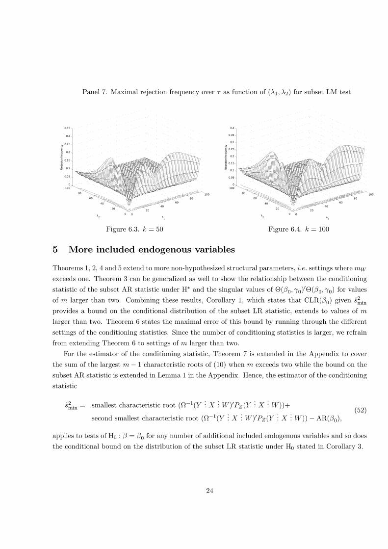
Panel 7. Maximal rejection frequency over � as function of (�1; �2) for subset LM test

020

4060

80100

0

20

40

60

80

1000

0.05

0.1

0.15

0.2

0.25

0.3

0.35

λ1λ2

Rej

ectio

n fre

quen

cy

020

4060

80100

0

20

40

60

80

1000

0.05

0.1

0.15

0.2

0.25

0.3

0.35

0.4

λ1λ2

Rej

ectio

n fre

quen

cy

Figure 6.3. k = 50 Figure 6.4. k = 100

5 More included endogenous variables

Theorems 1, 2, 4 and 5 extend to more non-hypothesized structural parameters, i:e: settings wheremW

exceeds one. Theorem 3 can be generalized as well to show the relationship between the conditioning

statistic of the subset AR statistic under H� and the singular values of �(�0; 0)0�(�0; 0) for values

of m larger than two. Combining these results, Corollary 1, which states that CLR(�0) given s2min

provides a bound on the conditional distribution of the subset LR statistic, extends to values of m

larger than two. Theorem 6 states the maximal error of this bound by running through the di¤erent

settings of the conditioning statistics. Since the number of conditioning statistics is larger, we refrain

from extending Theorem 6 to settings of m larger than two.

For the estimator of the conditioning statistic, Theorem 7 is extended in the Appendix to cover

the sum of the largest m� 1 characteristic roots of (10) when m exceeds two while the bound on the

subset AR statistic is extended in Lemma 1 in the Appendix. Hence, the estimator of the conditioning

statistic

~s2min = smallest characteristic root (�1(Y... X

... W )0PZ(Y... X

... W ))+

second smallest characteristic root (�1(Y... X

... W )0PZ(Y... X

... W ))�AR(�0);(52)

applies to tests of H0 : � = �0 for any number of additional included endogenous variables and so does

the conditional bound on the distribution of the subset LR statistic under H0 stated in Corollary 3.

24

Range of values of the estimator of the conditioning statistic. The estimator of the condi-

tioning statistic in (52) is a function of the subset AR statistic. Before we determine some properties

of ~s2min; we therefore �rst analyze the behavior of the realized value of the joint AR statistic that tests

H� : � = �0; = 0 as a function of � = (�00

... 00)0:

Theorem 11. Given a sample of N observations, the realized value of the joint AR statistic that

tests H � : � = �0; with � = (�0... 0)0 :

ARH�(�) = 1�""(�)

(y � ~X�)0PZ(y � ~X�);

is a function of � that has a minimum, maximum and (m� 1) saddle points. The values of the ARstatistic at these stationarity points are equal to resp. the smallest, largest and, if m exceeds one, the

second up to m-th root of the characteristic polynomial (10).


Theorem 11 implies that in a linear IV regression model with one included endogenous variable,

the realized value of the AR statistic when considered as a function of the structural parameters has

one minimum and one maximum while in linear IV models with more included endogenous variables,

it also has (m� 1) saddle points. Saddle points are stationary points at which the Hessian is positivede�nite in a number of directions and negative de�nite in the remaining directions. The saddle point

with the lowest value of the joint AR statistic therefore results from maximizing in one direction

and minimizing in all other (m � 1) directions. The subset AR statistic that tests H0 results from

minimizing the joint AR statistic over at � = �0: The maximal value of the subset AR statistic

is therefore smaller than or equal to the smallest value of the joint AR statistic over the di¤erent

saddle points since it results from constrained optimization (because of the ordering of the variables

where you optimize over). When m = 1; the optimization is unconstrained, since no minimization is

involved, so the maximal value of the subset AR statistic is equal to the second smallest characteristic

root which is in that case also the largest characteristic root.

Corollary 4. Given a sample of N observations, the maximum over all realized values of the subset

AR statistic is less than or equal to the second smallest characteristic root of (10):

max� AR(�) � second smallest root (�1(Y... X

... W )0PZ(Y... X

... W )): (53)

Corollary 5. Given a sample of N observations, the minimum over all realized values of the condi-

tioning statistic ~s2min is larger than or equal to the smallest characteristic root of (10):

min� ~s2min � smallest root (�1(Y

... X... W )0PZ(Y

... X... W )): (54)

25

Corollary 5 shows that the behavior of the conditioning statistic as a function of � for larger values

of m is similar to that when m = 1:

6 Testing at distant values

An important application of subset tests is to construct con�dence sets. Con�dence sets result from

specifying a grid of values of �0 and computing the subset statistic for each value of �0 on the grid.6

The (1 � �) � 100% con�dence set then consists of all values of �0 on the grid for which the subset

test is less than its 100 � �% critical value. These con�dence sets show that the subset LR test of

H0 : � = �0 at a value of �0 that is distant from the true one is identical to the subset LR test of

H : = 0 at a value of 0 that is distant from the true one and the same holds true for the subset

AR test.

Theorem 12. Given a sample of N observations, mx = 1; and for tests of H 0 : � = �0 for values of

�0 that are distant from the true value:

a. The realized value of the subset AR statistic AR(�0) equals the smallest eigenvalue of � 120

XW (X... W )0PZ(X

... W )� 12

XW ; with XW =

�!XX!WX

... !XW!WW

�:

b. The realized value of the subset LR statistic equals

LR(�0) = �min � �min; (55)

with �min the smallest eigenvalue of � 120

XW (X... W )0PZ(X

... W )� 12

XW and �min the smallest

eigenvalue of (10).

c. The realized value of the conditioning statistic s2min equals

s2min = smallest characteristic root (�1(Y... X

... W )0PZ(Y... X

... W ))+

second smallest characteristic root (�1(Y... X

... W )0PZ(Y... X

... W ))�

smallest characteristic root (�1XW (X... W )0PZ(X

... W )):

(56)


Theorem 12 shows that the expressions of the subset AR and LR statistics at values of �0 that are

distant from the true value do not depend on �: Hence, the same value of the statistics result when

6The con�dence sets that result from the subset tests can not (yet) be constructed using the e¢ cient proceduresdeveloped by Dufour and Taamouti (2003) for the AR statistic and Mikusheva (2007) for the LR statistic since theseapply to tests on all structural parameters.

26

we use them to test for a distant value of any element of : The weak identi�cation of one structural

parameter therefore carries over to all the other structural parameters. Hence, when the power for

testing one of the structural parameters is low because of its weak identi�cation, it is low for all other

structural parameters as well.

The smallest eigenvalue of � 120

XW (X... W )0PZ(X

... W )� 12

XW is identical to Anderson�s (1951) canon-

ical correlation reduced rank statistic which is the LR test under homoskedastic normal disturbances

of the hypothesis Hr : rank(�W... �X) = mw +mx� 1; see Anderson (1951). Thus Theorem 12 shows

that the subset AR test is equal to a reduced rank test of (�W... �X) at values of �0 that are distant

from the true one. Since the identi�cation condition for � and is that (�W... �X) has a full rank

value, the subset AR test at distant values of �0 is identical to a test for the identi�cation of � and :

7 Weak instrument setting

For ease of exposition, we have assumed sofar that the instruments are pre-determined and u and V

are jointly normal distributed with mean zero and a known value of the (reduced form) covariance

matrix . Our results extend straightforwardly to i.i.d. errors, instruments that are (possibly) random

and an unknown covariance matrix : The analogues of the subset AR and LR statistics in De�nition

1 for an unknown value of are obtained by replacing in these expressions by the estimator:

= 1N�k (y

... X... W )0MZ(y

... X... W ); (57)

which is a consistent estimator of under the outlined conditions, !p:

We next specify the parameter space for the null data generating processes.

Assumption 1. The parameter space under H 0 is such that:

= f = f 1; 2g : 1 = ( ; �W ; �X); 2 Rmw ; �W 2 Rk�mw ; �X 2 Rk�mx ; 2 = F : E(jjTijj2+�) < M; for Ti 2 f"i; Vi; Zi; Zi"i; ZiV 0i ; "iVig;

E(Zi"i) = 0; E(ZiV0i ) = 0; E((vec(Zi("i

... V 0i ))(vec(Z0i("i

... V 0i ))0) =

(E(("i... V 0i )

0("i... V 0i )) E(ZiZ 0i)) = (�Q); � =

0B@ 1 0 0

��0 1 0

0 1

1CA0

0B@ 1 0 0

��0 1 0

0 1

1CA9>>=>>; ;

(58)

for some � > 0; M < 1; Q = E(ZiZ0i) positive de�nite and 2 R(m+1)�(m+1) positive de�nite

symmetric.

Assumption 2 is a common parameter space assumption, see e.g. Andrews and Cheng (2012),

Andrews and Guggenberger (2009) and Guggenberger et al. (2012, 2019).

27

To determine the asymptotic size of the subset LR test, we analyze parameter sequences in

which lead to the speci�cation of the model for a sample of N i.i.d. observations as

yn = Xn� +Wn n + "n

Xn = Zn�X;n + VX;n

Wn = Zn�W;n + VW;n;

(59)

with yn : n � 1; Xn : n �mx; Wn : n �mw; Zn : n � k; "n : n � 1; VX;n : n �mx; VW;n : n �mw;

� : mx � 1; n : mw � 1; �X;n : k �mx; �W;n : k �mw: The rows of ("n... VX;n

... VW;n... Zn) are i.i.d.

distributed with distribution Fn: The mean of the rows of ("n... VX;n

... VW;n... Zn) equals zero and their

covariance matrix is

�n =

��"";n�V ";n

... �"V;n�V V;n

�: (60)

These sequences are assumed to allow for a singular value decomposition, see e:g: Golub and Van Loan

(1989), of the normalized reduced form parameter matrix.

Assumption 2. The matrix �(n) = (Z 0nZn)� 12 (�W;n

... �X;n)��1=2V V:";n that results from a sequence

�n = ( n; �W;n; �X;n; Fn) of null data generating processes in has a singular value decomposition:

�(n) = (Z 0nZn)� 12 (�W;n

... �X;n)��1=2V V:";n = HnTnR

0n 2 Rk�m; (61)

where Hn and Rn are k�k and m�m dimensional orthonormal matrices and Tn a k�n rectangularmatrix with the m singular values (in decreasing order) on the main diagonal, with a well de�ned

limit.

Theorem 13 states that the subset LR test is size correct for weak instrument settings.

Theorem 13. Under Assumptions 1 and 2, the asymptotic size of the subset LR test of H 0 with

signi�cance level � :

AsySzLR,� = lim supn!1 sup�2 Pr�hLRn(�0) > CLR1��(�0js2min = ~s2min;n)

i; (62)

where LRn(�0) is the subset LR statistic for a sample of size n and CLR1��(�0js2min = ~s2min) is the

(1��)� 100% quantile of the conditional distribution of CLR(�0) given that s2min = ~s

2min; is equal to

� for 0 < � < 1:


Equality of the rejection frequency of the subset LR test and the signi�cance level occurs when

is well identi�ed. When becomes less well identi�ed, the subset LR test, identical to the subset AR

test, becomes conservative.

28

8 Power comparison

We focus in our power comparison on the size-correct subset LR and subset AR tests where for the

latter we use both the conditional critical values from Guggenberger et al. (2019) and �2(k�1) criticalvalues. In Guggenberger et al. (2019), a power bound for the subset AR test is constructed and it

is shown that the rejection frequencies of the subset AR test when using their conditional critical

value function, are near this power bound. The subset AR statistic tests H0 by means of a reduced

rank restriction which H0 imposes on a matrix. The subset AR statistic therefore equals the smallest

characteristic root of the estimator of that matrix. A power bound for the subset AR test can then

be constructed using a LR statistic which tests conveniently speci�ed hypotheses on all characteristic

roots with the algorithms from Andrews et al. (2008) and Elliot et al. (2015). This LR test further

uses the closed form expression of the joint density of the estimators of the characteristic roots.

To show the di¤erences in the (alternative) hypotheses for the subset AR and subset LR tests, we

explicitly state the null and alternative hypotheses for both tests:

AR:

8>>>><>>>>:H0 : � = �0 (y �X�0

... W ) = Z�W ( ... ImW ) + (u

... VW )

H1 : � 6= �0 (y �X� +X(� � �0)... W ) = (u+ VX(� � �0))+

Z

��W (

... ImW ) + �X((� � �0)... 0)�

LR:

8>>>><>>>>:H0 : � = �0 (y �X�0

... W ) = Z�W ( 0... ImW ) + (u

... VW )

H1 : � 6= �0 (y �X� +X(� � �0)... W

... X) = (u+ VX(� � �0)... VW

... VX)+

Z

��W ( 0

... ImW... 0) + �X((� � �0)

... 0... ImX )

�(63)

It shows that for the subset AR test, the null and alternative hypothesis are reduced rank vs. full

rank values of the parameter matrix in the linear regression model:7

(y �X�0... W ) = Z�W + (u

... VW ); (64)

with �W a k � (mW + 1) dimensional matrix. The null and alternative hypothesis can then also be

speci�ed using the characteristic roots of the quadratic form of (scaled) �W for which a closed-form

expression of the joint density of their estimators is available. This allows Guggenberger et al. (2019)

to construct a power bound for the subset AR test.

Contrary to the subset AR test, the null and alternative hypothesis for the subset LR test both

imply reduced rank values for the parameter matrix in the linear regression model

(y �X�0... W

... X) = Z�+ (u... VW

... VX); (65)

7This shows that the subset AR test has no discriminatory power when �W and �X are linearly dependent, thesetting where the subset LM statistic is size distorted.

29

with � a k� (m+1) dimensional matrix. The null hypothesis, however, imposes a reduced rank valueon just the �rst (mW +1) columns of � while the alternative hypothesis imposes this restriction on the

combined columns of �: This means that we have to use all three elements of the concentration matrix

and the value of � under the alternative hypothesis to characterize the di¤erence between the null and

alternative hypothesis being tested using the subset LR test. Furthermore, no closed-form expression

is available for the density of the quadratic form of the estimator of � which has a non-central Wishart

distribution. This all considerably complicates the computation of power bounds for the subset LR

test compared to the subset AR test which we therefore refrain from.

Subset LR vs subset AR with �2(k�1) critical values We conduct a simulation study based on

the data generating process from Section 4, where we used a grid over (�1; �2; �) for a given number

of instruments, to analyze power. We restrict � ; which re�ects the dependence between �W and �X ;

to zero so �1 re�ects the identi�cation strength of � and �2 of : We use two di¤erent settings for the

number of instruments, �ve and twenty. Alongside the twenty-�ve point grids over �1 and �2; we use

a �fty-one point grid over � ranging from minus one to one while our null hypothesis is H0 : � = 0:

For every point on the grid, we use 2500 simulations.

We �rst compare the power of the subset LR test with that of the subset AR test when using

�2(k �mw) critical values. Guggenberger et al: (2012) show that this distribution provides a bound

on the distribution of the subset AR test. Panels 8 and 9 show the di¤erence in the rejection frequency

of testing H0 : � = 0 against H1 : � 6= 0 at the 95% signi�cance level between the subset LR and

subset AR tests. This di¤erence is re�ected as a function of � and the strength of identi�cation of

� re�ected by �2; for two di¤erent numbers of instruments k; 5 and 20, and two di¤erent strengths

of identi�cation of ; very weak �1 = 4 and semi-strong �1 = 25: The power of the subset LR test

dominates the power of the subset AR test using �2(k �mw) critical values for all our settings of �;

�1 and �2:

30

Panel 8. Di¤erence in rejection frequency of testing H0 : � = 0 against H1 : � 6= 0at the 95% signi�cance level between the subset LR and subset AR test using �2(k � 1)

critical values as a function of � and �2 (the identi�cation strength of �); k = 5

1

0.5

0

0.5

1

0

20

40

60

80

100

0

0.005

0.01

0.015

0.02

0.025

0.03

βλ21

0.5

0

0.5

1

0

20

40

60

80

1000

0.05

0.1

0.15

0.2

0.25

0.3

βλ2

Figure 8.1. �1 = 4 (identi�cation of ) Figure 8.2. �1 = 25 (identi�cation of )

Panel 9. Di¤erence in rejection frequency of testing H0 : � = 0 against H1 : � 6= 0at the 95% signi�cance level between the subset LR and subset AR test using �2(k � 1)critical values as a function of � and �2 (the identi�cation strength of �); k = 20

1

0.5

0

0.5

1

0

20

40

60

80

1000.005

0

0.005

0.01

0.015

0.02

0.025

0.03

0.035

0.04

βλ21

0.5

0

0.5

1

0

20

40

60

80

1000

0.05

0.1

0.15

0.2

0.25

0.3

βλ2


Subset LR vs subset AR with conditional critical values We next compare the power dif-

ference of testing H0 : � = 0 against H1 : � 6= 0 using the subset LR and the subset AR test with

conditional critical values from Guggenberger et al. (2019). Panels 10 and 11 are for the same settings

as Panels 8 and 9. When compared to these panels, the subset LR test is now slightly less powerful

31

when the non-hypothesized parameter, ; is (very) weakly identi�ed and generally more powerful when

it is (reasonably) well identi�ed.

Panel 10. Di¤erence in rejection frequency of testing H0 : � = 0 against H1 : � 6= 0at the 95% signi�cance level between the subset LR and subset AR test using conditional


1

0.5

0

0.5

1

0

20

40

60

80

1000.05

0.045

0.04

0.035

0.03

0.025

0.02

0.015

0.01

βλ21

0.5

0

0.5

1

0

20

40

60

80

100

0

0.05

0.1

0.15

0.2

βλ2




1

0.5

0

0.5

1

0

20

40

60

80

1000.06

0.05

0.04

0.03

0.02

0.01

0

βλ21

0.5

0

0.5

1

0

20

40

60

80

100

0

0.05

0.1

0.15

0.2

βλ2


To further analyze the di¤erence in power between the subset LR test and the subset AR test

with conditional critical values, Panels 12 and 13 show the di¤erence in the rejection frequencies for

32

tests of H0 : � = 0 against H1 : � 6= 0 using the subset LR and AR tests for di¤erent numbers of

instruments and identi�cation strengths of �; as a function of � and the identi�cation strength of :

Figures 12.1 and 13.1 show that for very weakly identi�ed settings of �; were power is very low in

general, the subset AR test is slightly more powerful than the subset LR test. Figures 12.2 and 13.2

show that when � is reasonably well identi�ed that the subset LR is more powerful except when is

very weakly identi�ed. The equal rejection frequency lines of testing using subset LR or subset AR

resulting from Figures 12.2 and 13.2 are shown in Panel 14. They are remarkably similar and show

again that when is weakly identi�ed, so power is low, that the subset AR test is (slightly) more

powerful than the subset LR test. For reasonable small identi�cation strengths of ; the subset LR

test, however, dominates in terms of power.


critical values as a function of � and �1 (the identi�cation strength of ); k = 5

1

0.5

0

0.5

1

0

20

40

60

80

1000.05

0.04

0.03

0.02

0.01

0

0.01

0.02

βλ11

0.5

0

0.5

1

0

20

40

60

80

1000.05

0

0.05

0.1

0.15

0.2

0.25

βλ1

Figure 12.1. �2 = 4 (identi�cation of �) Figure 12.2. �2 = 25 (identi�cation of �)

33


critical values as a function of � and �1 (the identi�cation strength of ); k = 20

1

0.5

0

0.5

1

0

20

40

60

80

100

0.04

0.03

0.02

0.01

0

0.01

0.02

βλ11

0.5

0

0.5

1

0

20

40

60

80

1000.05

0

0.05

0.1

0.15

0.2

0.25

βλ1

Figure 13.1. �2 = 4 (identi�cation of �) Figure 13.2. �2 = 25 (identi�cation of �)

Panel 14. Equal rejection frequency line for testing H0 : � = 0 against H1 : � 6= 0 at the95% signi�cance level when using the subset LR or subset AR test using conditional

critical values as a function of � and �1 (the identi�cation strength of ); �2 = 25

β

λ 1

1 0.8 0.6 0.4 0.2 0 0.2 0.4 0.6 0.8 10

10

20

30

40

50

60

70

80

90

100

β

λ 1

1 0.8 0.6 0.4 0.2 0 0.2 0.4 0.6 0.8 10

10

20

30

40

50

60

70

80

90

100

Figure 14.1. k = 5 Figure 14.2. k = 20

9 95% con�dence sets for return on education for Card (1995)

Card (1995) analyzes the return on education for earnings. He uses proximity to college as an in-

strument in an IV regression of (length of) education on (the log) wage. The proximity in�uences

34

InstrumentsnEstimation Method LS 2SLS LIMLage; age2; indicators for prox to 2, 4 and 4 year public college 0:074

0:00350:1620:041

0:180:048

Table 1: Estimates of return on education � (standard error is listed below).

the cost of college education so it is directly related to the (length of) education but only indirectly

(channeled by education) to earnings. We construct 95% con�dence sets for the return on education.

Since other endogenous variables are present in the structural equation, i.e. experience, experience2;

we use the subset LR, subset AR and subset LM tests to do so. The data set of Card (1995) consists

of 3010 observations obtained from the 1976 subsample of the National Longitudinal Survey of Young

Men. Our data consists of: four variables indicating the proximity to college, the length of education,

log-wages, experience and age, metropolitan, family and regional indicators. For more details on the

data we refer to Card (1995).

The model that is used by Card is identical to model (1) expanded with an additional set of

exogenous control variables, i:e: a constant term and the racial, metropolitan, family and regional

indicator variables. Hence, the variables in (1) stand for: yi the (logarithm of the) wage of individual

i; Xi the length of education of individual i; Wi = (expi exp2i )0 contains the experience (exp) and

experience squared of individual i and the instrument vector Zi consists of age, age2 and three indicator

variables which show the proximity to a two year college, a four year college and a four year public

college respectively. The experience variables are obtained from age and education: expi =agei�6�Yi:All these variables are regressed on the exogenous control variables and the residuals from these

regressions are used in the expressions of our test statistics.

Table 1 contains estimates of the return on education for three estimation procedures. Kleibergen

(2004) reports tests for the rank value of (�X... �W ) which show that the return on education is

weakly identi�ed so t-tests based on the estimators and standard errors reported in Table 1 have to be

interpreted with caution, see also Stock and Yogo (2001). Since three included endogenous variables

are present, we use the subset LR, subset AR and subset LM tests to construct 95% con�dence sets

for the return on education. The conditioning statistic for the conditional critical value function of

the subset LR test is computed using (52) which applies to settings where mW exceeds one. For the

conditioning statistic of the subset AR test, we use the extension provided by Guggenberger et al:

(2019) for mW larger than one. It implies, however, that the conditioning statistic is very large so the

conditional critical value function becomes identical to the �2(3) critical value function.

35

Figure 15. Tests of H0 : � = �educ using subset LR (solid), subset LM (dashed) and

subset AR (dash-dotted line) and their 95% (conditional) critical value lines (dotted).

0 0.05 0.1 0.15 0.2 0.25 0.3 0.35 0.4 0.45 0.50

2

4

6

8

10

12

14

16

18

20

βeduc

Test

statis

tics

Figure 15.1: return on education

Figure 15 shows the values of the subset LR, subset AR and subset LM tests as a function of the

hypothesized value of the return on education parameter. Figure 15 also shows the 95% critical value

function of these statistics whose intersections with them (indicated by the straight vertical lines) show

the resulting 95% con�dence sets. The 95% con�dence set that results from the subset LR test is the

shortest while the one from the subset LM test is the longest. The latter test is also not size correct

for all settings of the nuisance parameters, see Guggenberger et al. (2012). These 95% con�dence sets

di¤er substantially from the one that results from the two stage least squares t-test which is much too

tight: (0.082, 0.24). This again reiterates the importance of using size correct subset tests.

10 Conclusions

Inference using the LR test on one structural parameter in the homoskedastic linear IV regression

model extends straightforwardly from a model with just one included endogenous variable to several.

The �rst and foremost extension is that of the conditional critical value function. When using the usual

degrees of freedom adjustments of the involved �2 distributed random variables to account for the

parameters left unrestricted by the hypothesis of interest, the conditional critical value function of the

LR test in the linear IV regression model with one included endogenous variable from Moreira (2003)

provides a bounding critical value function for the subset LR test of a hypothesis on one structural

parameter of several in a linear IV regression model with multiple included endogenous variables. The

functional expression of the conditioning statistic involved in the conditional critical value function is

36

unaltered. This speci�cation of the conditional critical value function and its conditioning statistic

makes the LR test for one structural parameter size correct.

A second important property of the conditional critical value function is optimality of the resulting

subset LR test under strong identi�cation of all untested structural parameters. When all untested

structural parameters are well identi�ed, the subset LR test becomes identical to the LR test in the

linear IV regression model with one included endogenous variable for which Andrews et al. (2006)

show that the LR test is optimal under weak and strong identi�cation of the hypothesized structural

parameter. Establishing optimality while allowing for any kind of identi�cation strength for the

untested parameters is complicated. In Guggenberger et al. (2019), conditional critical values for

the subset AR statistic are constructed which make it nearly optimal under weak instruments for

the untested structural parameters but not so under strong instruments and over identi�cation. A

simulation experiment shows that for such weak identi�cation settings this subset AR test indeed

(slightly) dominates our subset LR test in terms of power but the subset LR test starts to dominate

for just minor amounts of identi�cation of the structural parameters.

A key property of the homoskedastic linear IV regression model is the reduced rank structure it

imposes on the reduced form parameter matrix. Our results for the subset LR test in the homoskedastic

linear IV regression model therefore directly extend to LR tests on subsets of the structural parameters

in other homoskedastic models that also imply such a reduced rank structure. A prominent example

of such a model is the linear factor model in asset pricing that is used to determine the expected

asset return premium on risk factors. For many empirical factors used in the literature, these risk

premia are, however, weakly identi�ed, see Kleibergen (2009). It is also common to estimate several

risk premia so our proposed subset LR test is also important for constructing con�dence sets for risk

premia in asset pricing.

References

[1] Anderson, T.W. Estimating linear restrictions on regression coe¢ cients for multivariate normal

distributions. Annals of Mathematical Statistics, 22:327�351, 1951.

[2] Anderson, T.W. and H. Rubin. Estimation of the Parameters of a Single Equation in a Complete

Set of Stochastic Equations. The Annals of Mathematical Statistics, 21:570�582, 1949.

[3] Anderson, T.W., N. Kunitomo, and T. Sawa. Comparison of the Densities of the TSLS and

LIMLK estimators for Simultaneous Equations. In F.G. Adams and B.G. Hickman, editor, Global

Econometrics: Essays in Honor of Lawrence R. Klein, pages 102�124. MIT Press, 1983.

[4] Andrews. D.W.K. and P. Guggenberger. Hybird and Size-Corrected Subsampling Methods.

Econometrica, 3:721�762, 2009.

37

[5] Andrews, D.W.K. and X. Cheng. Estimation and inference with Weak, Semi-Strong and Strong

Identi�cation. Econometrica, 80:2153�2211, 2012.

[6] Andrews, D.W.K., M.J. Moreira and J.H. Stock. Optimal Two-Sided Invariant Similar Tests for

Instrumental Variables Regression. Econometrica, 74:715�752, 2006.

[7] Andrews, D.W.K., M.J. Moreira and J.H. Stock. E¢ cient two-sided nonsimilar invariant tests in

IV regression with weak instruments. Journal of Econometrics, 146:241�254, 2008.

[8] Andrews, I. Conditional Linear Combination Tests for Weakly Identi�ed Models. Econometrica,

84:2155�2182, 2016.

[9] Card, D. Using geographic variation in college proximity to estimate the return to schooling. In

L.N. Christo�des, E.K. Grant and R. Swidinsky, editor, Aspects of Labour Market Behaviour: es-

says in honor of John Vanderkamp, pages 201�222. University of Toronto Press, Toronto, Canada,

1995. (NBER Working Paper 4483 (1993)).

[10] Chernozhukov,V., C. Hansen and M. Jansson. Admissible Invariant Similar Tests for Instrumental

Variables Regression. Econometric Theory, 25, 2009.

[11] Dufour, J.-M. and M. Taamouti. Projection-based statistical inference in linear structural models

with possibly weak instruments. Econometrica, 73:1351�1365, 2005.

[12] Elliot, G., U.K. Müller and M.W. Watson. Nearly optimal tests when a nuisance parameter is

present under the null hypothesis. Econometrica, 83:771�811, 2015.

[13] Golub, G.H. and C.F. van Loan. Matrix Computations. The John Hopkins University Press

(Baltimore), 1989.

[14] Guggenberger, P. , F. Kleibergen, S. Mavroeidis, and L. Chen. On the asymptotic sizes of

subset anderson-rubin and lagrange multiplier tests in linear instrumental variables regression.

Econometrica, 80:2649�2666, 2012.

[15] Guggenberger, P., F. Kleibergen and S. Mavroeidis. A more powerful Anderson Rubin test in

linear instrumental variables regression. Quantitative Economics, 2019. Forthcoming.

[16] Kleibergen, F. Pivotal Statistics for testing Structural Parameters in Instrumental Variables

Regression. Econometrica, 70:1781�1803, 2002.

[17] Kleibergen, F. Testing Subsets of Structural Parameters in the Instrumental Variables Regression

Model. Review of Economic and Statistics, 86:418�423, 2004.

[18] Kleibergen, F. Testing Parameters in GMM without assuming that they are identi�ed. Econo-

metrica, 73:1103�1124, 2005.

38

[19] Kleibergen, F. Generalizing weak instrument robust IV statistics towards multiple parameters,

unrestricted covariance matrices and identi�cation statistics. Journal of Econometrics, 139:181�216, 2007.

[20] Kleibergen, F. Tests of Risk Premia in Linear Factor Models. Journal of Econometrics, 149:149�173, 2009.

[21] Mikusheva, A. Robust Con�dence Sets in the Presence of Weak Instruments. Journal of Econo-

metrics, 157(236-247), 2010.

[22] Montiel Olea, J. L. E¢ cient conditionally similar tests �nite-sample theory and large-sample

applications. Working Paper, New York University, 2015.

[23] Moreira, H. and M.J. Moreira. Contributions to the Theory of Optimal Tests. Working paper,

Getulio Vargas Foundation, 2015.

[24] Moreira, M.J.,. A Conditional Likelihood Ratio Test for Structural Models. Econometrica,

71:1027�1048, 2003.

[25] Stock, J.H. and M. Yogo. Testing for Weak Instruments in Linear IV Regression. In D.W.K.

Andrews and J.H. Stock, editor, Identi�cation and Inference for Econometric Models: Essays

in Honor of Thomas Rothenberg, pages 80�108. Cambridge: Cambridge University Press, 2005.

Prepared for Festschrift in honor of Thomas Rothenberg.

39

Appendix for: E¢ cient size correct subset inference inhomoskedastic linear instrumental variables regression

Lemma 1. a. The distribution of the subset AR statistic (5) for testing H 0 : � = �0 is bounded

according to

AR (�0) ��(�0; 0)

0M�(�0; 0)(Imw0 )

�(�0; 0)

1+'0h(Imw0 )

0�(�0; 0)

0�(�0; 0)(Imw0 )

i�1'� �(�0; 0)

0M�(�0; 0)(

Imw0 )

�(�0; 0)

= �0� + � 0� � �2(k �mw):

(66)

b. When mw = 1; we can specify the subset AR statistic as

AR(�0) � (�0� + �2)��1� '2

'2+(Imw0 )0�(�0; 0)

0�(�0; 0)(Imw0 )

�� e (67)

with

e = 2

v�(�0; 0)

0M�(�0; 0)(Imw0 )

�(�0; 0)

v2+(Imw0 )0�(�0; 0)

0�(�0; 0)(Imw0 )

!2(Imw0 )

0�(�0; 0)

0�(�0; 0)(Imw0 )

v2+(Imw0 )0�(�0; 0)

0�(�0; 0)(Imw0 )(

1��(�0; 0)

0M�(�0; 0)(Imw0 )

�(�0; 0)

v2+(Imw0 )0�(�0; 0)

0�(�0; 0)(Imw0 )

+4�(�0; 0)

0M�(�0; 0)(Imw0 )

�(�0; 0)�v2+(Imw0 )

0�(�0; 0)

0�(�0; 0)(Imw0 )

�2)�1

;

(68)

so

e = O

0@ v�(�0; 0)0M

�(�0; 0)(Imw0 )�(�0; 0)

v2+(Imw0 )0�(�0; 0)

0�(�0; 0)(Imw0 )

!21A � 0: (69)

Proof. a. To obtain the approximation of the subset AR statistic, AR(�0); we use that it equalsthe smallest root of the characteristic polynomial:��(�0)� (y �X�0 ... W )0PZ(y �X�0 ... W )�� = 0:

We �rst pre- and post multiply the matrices in the characteristic polynomial by�1� 0

... 0ImW

�

40

to obtain �� 1� 0

... 0ImW

�0(�0)

�1� 0

... 0ImW

��

��

1� 0

... 0ImW

�0 �Z�W ( 0

... Imw) + ("... VW )

�1 0

... 0ImW

��0PZ

PZ

�Z�W ( 0

... Imw) + ("... VW )

�1 0

... 0ImW

��1� 0

... 0ImW

�� = 0,��W ��"... Z�W + VW

�0PZ

�"... Z�W + VW

�� = 0:

where �W =

�1� 0

... 0ImW

�0(�0)

�1� 0

... 0ImW

�: We now specify �

� 12

W as

�� 12

W =

�� 12

""0

...��1"" �"W�

� 12

ww:"

�� 12

ww:"

!

with �WW:" = �WW � �W"��1"" �"W ; so we can specify the characteristic polynomial as well as:�� 1

20

W �W�� 12

W � ��120

W

�"... Z�W + VW

�0PZ

�"... Z�W + VW

�� 12

W

�� = 0,��ImW+1 � ��(�0; 0) ... �(�0; 0)�Imw0 ��0 ��(�0; 0) ... �(�0; 0)�Imw0 �� = 0

with � =��""�V "

... �"V�V V

�; with �"" : 1� 1; �V " = �0"V : m� 1 and �V V : m�m;

�� 120

V V:" =

�� 12

WW:"

��12

XX:(" : W )�XW:"�

�1WW:"

...0

�� 12

XX:(" : W )

!;

�WW:" = �WW ��W"��1"" �"W ; �XW:" = �XW ��X"��1"" �"W ; �XX:(" : W ) = �XX�

��"X�WX

�0��1W

��"X�WX

�:

We note that �(�0; 0) and �(�0; 0) are independently distributed since0@ �� 12

"" ��"V�""�� 12

V V:"

0 �� 12

V V:"

1A0�0@ �

� 12

"" ��"V�""�� 12

V V:"

0 �� 12

V V:"

1Ais block diagonal. Returning to the characteristic polynomial, it reads��ImW+1 � ��(�0; 0) ... �(�0; 0)�Imw0 ��0 ��(�0; 0) ... �(�0; 0)�Imw0 �� = 0,��ImW+1 � � �(�0; 0)

0�(�0; 0)

(Imw0 )0�(�0; 0)

0�(�0; 0)

...�(�0; 0)

0�(�0; 0)(Imw0 )

(Imw0 )0�(�0; 0)

0�(�0; 0)(Imw0 )

�� = 0:

41

We specify�

�(�0; 0)0�(�0; 0)

(Imw0 )0�(�0; 0)

0�(�0; 0)

...�(�0; 0)

0�(�0; 0)(Imw0 )

(Imw0 )0�(�0; 0)

0�(�0; 0)(Imw0 )

�as follows

��(�0; 0)

0�(�0; 0)

(Imw0 )0�(�0; 0)

0�(�0; 0)

...�(�0; 0)

0�(�0; 0)(Imw0 )

(Imw0 )0�(�0; 0)

0�(�0; 0)(Imw0 )

�=

=

�10

...�(�0; 0)

0�(�0; 0)(Imw0 )

h(Imw0 )

0�(�0; 0)

0�(�0; 0)(Imw0 )

i�1Imw

��(�0; 0)

0M�(�0; 0)(Imw0 )

�(�0; 0)

0

... 0

(Imw0 )0�(�0; 0)

0�(�0; 0)(Imw0 )

��10

...�(�0; 0)

0�(�0; 0)(Imw0 )

h(Imw0 )

0�(�0; 0)

0�(�0; 0)(Imw0 )

i�1Imw

�0=

10

...v0h(Imw0 )

0�(�0; 0)

0�(�0; 0)(Imw0 )

i� 12

Imw

!��(�0; 0)

0M�(�0; 0)(Imw0 )

�(�0; 0)

0

... 0

(Imw0 )0�(�0; 0)

0�(�0; 0)(Imw0 )

��

1h(Imw0 )

0�(�0; 0)

0�(�0; 0)(Imw0 )

i� 12 v

... 0Imw

�;

with ' =h�Imw0

�0�(�0; 0)

0�(�0; 0)�Imw0

�i� 12 �Imw

0

�0�(�0; 0)

0�(�0; 0)!dN(0; Imw) and independent

of �(�0; 0)0M

�(�0; 0)(Imw0 )

�(�0; 0) and�Imw0

�0�(�0; 0)

0�(�0; 0)�Imw0

�; which are independent of one

another as well, so the characteristic polynomial becomes:��ImW+1 � 10

...'0h(Imw0 )

0�(�0; 0)

0�(�0; 0)(Imw0 )

i� 12

Imw

!��(�0; 0)

0M�(�0; 0)(Imw0 )

�(�0; 0)

0

...

... 0

(Imw0 )0�(�0; 0)

0�(�0; 0)(Imw0 )

��1h

(Imw0 )0�(�0; 0)

0�(�0; 0)(Imw0 )

i� 12 '

... 0Imw

�� = 0:

We can construct a bound on the smallest root of the above polynomial by noting that the smallest

root coincides with

minc

"1

( 1�c)0( 1�c)

�1�c�0 1

0

...'0h(Imw0 )

0�(�0; 0)

0�(�0; 0)(Imw0 )

i� 12

Imw

!��(�0; 0)

0M�(�0; 0)(Imw0 )

�(�0; 0)

0

...

... 0

(Imw0 )0�(�0; 0)

0�(�0; 0)(Imw0 )

��1h

(Imw0 )0�(�0; 0)

0�(�0; 0)(Imw0 )

i� 12 '

... 0Imw

��1�c��:

If we use a value of c equal to

~c =h�Imw0

�0�(�0; 0)

0�(�0; 0)�Imw0

�i� 12'

and substitute it into the above expression, we obtain an expression that is always larger than or equal

to the smallest root, i:e: the subset AR statistic, since this is the minimal value with respect to c; see

42

Guggenberger et al. (2012),

AR(�0) ��(�0; 0)

0M�(�0; 0)(Imw0 )

�(�0; 0)

1+'0h(Imw0 )

0�(�0; 0)

0�(�0; 0)(Imw0 )

i�1'= �0�+�0�

1+'0h(Imw0 )

0�(�0; 0)

0�(�0; 0)(Imw0 )

i�1'

� �0� + � 0� � �2(k �mw):

This shows that the subset AR statistic is less than or equal to a �2(k � mw) distributed random

variable. The upper bound on the distribution of the subset AR statistic coincides with its distribution

when �(�0; 0)�Imw0

�is large so it is a sharp upper bound.

b. We assess the approximation error when using the upper bound for AR(�0) when mw = 1: In order

to do so, we use that

AR(�0) = minc f(c);

with

f(c) =( 1�c)

0A( 1�c)

( 1�c)0( 1�c)

;

and

A =

10

...'0h(Imw0 )

0�(�0; 0)

0�(�0; 0)(Imw0 )

i� 12

Imw

!��(�0; 0)

0M�(�0; 0)(Imw0 )

�(�0; 0)

0

...

... 0

(Imw0 )0�(�0; 0)

0�(�0; 0)(Imw0 )

��1h

(Imw0 )0�(�0; 0)

0�(�0; 0)(Imw0 )

i� 12 '

... 0Imw

��1�c��:

:

The subset AR statistic evaluates f(c) at c while our approximation does so at ~c: To assess the

magnitude of the approximation error, we conduct a �rst order Taylor approximation:

f(c) � f (~c) +�@f@c j~c

�(c� ~c);

for which we obtain the expression of (c� ~c) from a �rst order Taylor approximation of�@f@c jc

�= 0 :

0 =�@f@c jc

��

�@f@c j~c

�+�@2f@c2j~c�(c� ~c),

c� ~c � ��@2f@c2j~c��1 �

@f@c j~c

�so upon combining:

f(c) � f (~c)��@2f@c2j~c��1 �

@f@c j~c

�2:

43

The expressions for the �rst and second order derivative of f(c) read:

@f@c = 2

�( 1�c)

0A( 0�1)

( 1�c)0( 1�c)

� (1�c)

0A( 1�c)

( 1�c)0( 1�c)

( 1�c)0( 0�1)

( 1�c)0( 1�c)

�@2f@c2

= 2

�( 0�1)

0A( 0�1)

( 1�c)0( 1�c)

� (1�c)

0A( 0�1)

( 1�c)0( 1�c)

( 1�c)0( 0�1)

( 1�c)0( 1�c)

� 2(1�c)

0A( 0�1)

( 1�c)0( 1�c)

( 1�c)0( 0�1)

( 1�c)0( 1�c)

+

4( 1�c)

0A( 1�c)

( 1�c)0( 1�c)

�( 1�c)

0( 0�1)

( 1�c)0( 1�c)

�2� (

1�c)

0A( 1�c)

( 1�c)0( 1�c)

( 0�1)0( 0�1)

( 1�c)0( 1�c)

#;

so using that�1�~c�0A�0�1�= 0;

�1�~c�0A�1�~c�= �(�0; 0)

0M�(�0; 0)(

Imw0 )

�(�0; 0);�1�~c�0� 1

�~c�= 1+'0

h�Imw0

�0�(�0; 0)

0�(�0; 0)�Imw0

�i�1';�

1�~c�0� 0

�1�=h�Imw0

�0�(�0; 0)

0�(�0; 0)�Imw0

�i� 12';�0�1�0A�0�1�=�Imw0

�0�(�0; 0)

0�(�0; 0)�Imw0

�; we

obtain that

@f@c j~c = �2

�(�0; 0)0M

�(�0; 0)(Imw0 )�(�0; 0)�

1+'0h(Imw0 )

0�(�0; 0)

0�(�0; 0)(Imw0 )

i�1'

�2 h�Imw0 �0�(�0; 0)0�(�0; 0)�Imw0 �i� 12'

@2f@c2j~c = 2

24 (Imw0 )0�(�0; 0)

0�(�0; 0)(Imw0 )�

1+'0h(Imw0 )

0�(�0; 0)

0�(�0; 0)(Imw0 )

i�1'

� � �(�0; 0)0M

�(�0; 0)(Imw0 )�(�0; 0)�

1+'0h(Imw0 )

0�(�0; 0)

0�(�0; 0)(Imw0 )

i�1'

�2+

4�(�0; 0)

0M�(�0; 0)(Imw0 )

�(�0; 0)�1+'0

h(Imw0 )

0�(�0; 0)

0�(�0; 0)(Imw0 )

i�1'

� '0h(Imw0 )

0�(�0; 0)

0�(�0; 0)(Imw0 )

i�1'�

1+'0h(Imw0 )

0�(�0; 0)

0�(�0; 0)(Imw0 )

i�1'

�235

= 2�(�0; 0)

0M�(�0; 0)(Imw0 )

�(�0; 0)

1+'0h(Imw0 )

0�(�0; 0)

0�(�0; 0)(Imw0 )

i�1'

"(Imw0 )

0�(�0; 0)

0�(�0; 0)(Imw0 )

�(�0; 0)0M

�(�0; 0)(Imw0 )�(�0; 0)

�

1

1+'0h(Imw0 )

0�(�0; 0)

0�(�0; 0)(Imw0 )

i�1'+ 4

'0h(Imw0 )

0�(�0; 0)

0�(�0; 0)(Imw0 )

i�1'�

1+'0h(Imw0 )

0�(�0; 0)

0�(�0; 0)(Imw0 )

i�1'

�235 :

Hence,

�@2f@c2j~c��1 �

@f@c j~c

�2= 2

�(�0; 0)0M

�(�0; 0)(Imw0 )�(�0; 0)�

1+'0h(Imw0 )

0�(�0; 0)

0�(�0; 0)(Imw0 )

i�1'

�2 '0h(Imw0 )

0�(�0; 0)

0�(�0; 0)(Imw0 )

i�1'

1+'0h(Imw0 )

0�(�0; 0)

0�(�0; 0)(Imw0 )

i�1'"

(Imw0 )0�(�0; 0)

0�(�0; 0)(Imw0 )

�(�0; 0)0M

�(�0; 0)(Imw0 )�(�0; 0)

� 1

1+'0h(Imw0 )

0�(�0; 0)

0�(�0; 0)(Imw0 )

i�1'+

4'0h(Imw0 )

0�(�0; 0)

0�(�0; 0)(Imw0 )

i�1'�

1+'0h(Imw0 )

0�(�0; 0)

0�(�0; 0)(Imw0 )

i�1'

�235�1

44

and

AR(�0) � �(�0; 0)0M

�(�0; 0)(Imw0 )

�(�0; 0)��1� '2

'2+(Imw0 )0�(�0; 0)

0�(�0; 0)(Imw0 )�

2

'2�(�0; 0)

0M�(�0; 0)(Imw0 )

�(�0; 0)�'2+(Imw0 )

0�(�0; 0)

0�(�0; 0)(Imw0 )

�2!

(Imw0 )0�(�0; 0)

0�(�0; 0)(Imw0 )

'2+(Imw0 )0�(�0; 0)

0�(�0; 0)(Imw0 )(

1��(�0; 0)

0M�(�0; 0)(Imw0 )

�(�0; 0)

'2+(Imw0 )0�(�0; 0)

0�(�0; 0)(Imw0 )

+4�(�0; 0)

0M�(�0; 0)(Imw0 )

�(�0; 0)�'2+(Imw0 )

0�(�0; 0)

0�(�0; 0)(Imw0 )

�2)�135 ;

where we used that 1

1+'0h(Imw0 )

0�(�0; 0)

0�(�0; 0)(Imw0 )

i�1'=

(Imw0 )0�(�0; 0)

0�(�0; 0)(Imw0 )

'2+(Imw0 )0�(�0; 0)

0�(�0; 0)(Imw0 )

: It shows

that the error of approximating f(c) by f(~c) is of the order of

'�(�0; 0)

0M�(�0; 0)(Imw0 )

�(�0; 0)

'2+(Imw0 )0�(�0; 0)

0�(�0; 0)(Imw0 )

!2or

O(

'�(�0; 0)

0M�(�0; 0)(Imw0 )

�(�0; 0)

'2+(Imw0 )0�(�0; 0)

0�(�0; 0)(Imw0 )

!2):

Lemma 2. The derivative of the approximate conditional distribution of the subset LR statistic given

s2min = r (23) with respect to r is strictly larger than minus one and strictly smaller than zero.

Proof.

@@r12

��2 + �0� � r +

p(�2 + �0� + r)2 � 4r�0�

�= 1

2

��1 + �2��0�+rp

(�2��0�+r)2+4�2�0�

�since (�2 + �0� + r)2 � 4r�0� = (�2 � �0� + r)2 + 4�2�0� � (�2 � �0� + r)2; the derivative lies betweenminus one and zero:

�1 < 12

��1 + �2��0�+rp

(�2��0�+r)2+4�2�0�

�< 0:

The strict lowerbound on the derivative results since it is an increasing function of s2 :

@@r12

��1 + �2��0�+rp

(�2��0�+r)2+4�2�0�

�= 1

2p(�2+�0�+r)2�4r�0�

h1� (�2��0�+r)2

((�2+�0�+r)2�4r�0�)

i= 1p

(�2+�0�+r)2�4r�0�

h1� (�2��0�+r)2

(�2��0�+r)2+4�2�0�

i� 0

so its smallest value is attained at r = 0: When r = 0;

12

��1 + �2��0�p

(�2+�0�)2

�= 1

2

��1 + �2��0�p

(�2+�0�)2

�= 1

2

h�1 + �2��0�

�2+�0�

i= �1 + �2

�2+�0� > �1:

45

Proof of Theorem 1. The subset AR statistic equals the smallest root of (7). We �rst pre and

post multiply the characteristic polynomial by

1 0

� 0 ImW

!; which since

��

1 0

� 0 ImW

!�� = 1;does not change the value of the determinant:��(�0)� �Y �X�0 ... W�0 PZ �Y �X�0 ... W�� = 0 ,��

1 0

� 0 ImW

!0[�(�0)�

�Y �X�0

... W�0PZ

�Y �X�0

... W�]

1 0

� 0 ImW

!�� = 0 ,��WW ��Y �W 0 �X�0

... W�0PZ

�Y �W 0 �X�0

... W�� = 0:

We conduct a Choleski decomposition of �WW =

��""�VW "

... �"VW�VWVW

�; with �"" : 1� 1; �VW " = �0"VW :

m� 1 and �VWVW : mW �mW ;

�� 120

WW =

�� 12

""

��12

VWVW :"�VW "��1""

...0

�� 12

VWVW :"

!;

with �VWVW :" = �VWVW��VW "��1"" �"VW ; and use it to further transform the characteristic polynomial:��WW ��Y �W 0 �X�0

... W�0PZ

�Y �W 0 �X�0

... W�� = 0 ,�� 1

20

WW

��WW �

�Y �W 0 �X�0

... W�0PZ

�Y �W 0 �X�0

... W�� 12

WW

�� = 0 ,��Im+1 � ��(�0; 0) ... �(�0; 0)�ImW0 ��0��(�0; 0) ... �(�0; 0)�ImW0 �� = 0;with

�(�0; 0) = (Z0Z)�

12Z 0(y �W 0 �X�0)=�

12"";

�(�0; 0) = (Z0Z)�

12Z 0

�(W

... X)� (y �W 0 �X�0)�"V�""

�� 12

V V:"

46

and �V V:" = �V V ��V "��1"" �"V =��VWVW :"

�VXVW :"

... �VWVX:"

�VXVX:"

�; �VWVX :" = �

0VXVW :" : mW�mX ; �VWVX :" =

�0VXVX :" : mX �mX : Since mW = 1; we can now specify the characteristic polynomial as��

�� (�0; 0)0�(�0; 0) �(�0; 0)0�(�0; 0)

�ImW0

��ImW0

�0�(�0; 0)

0�(�0; 0) �� s�

!�� = 0,�� '0'� � 0� � �0� 's�

12

's�12 �� s�

!�� = 0,

�2 � �('0'+ � 0� + �0� + s�) + (�0� + � 0�)s� = 0;

with

' =h�Imw0

�0�(�0; 0)

0�(�0; 0)�Imw0

�i� 12 �Imw

0

�0�(�0; 0)

0�(�0; 0) � N(0; Imw)

� =h�

0ImX

�0[�(�0; 0)

0�(�0; 0)]�1 � 0

ImX

�i� 12�

0ImX

�0[�(�0; 0)

0�(�0; 0)]�1�(�0; 0)

0�(�0; 0)

� = �(�0; 0)0?�(�0; 0) � N(0; Ik�m)

s� =�Imw0

�0�(�0; 0)

0�(�0; 0)�Imw0

�so the smallest root is characterized by

12

�'2 + �2 + �0� + s� �

q('2 + �2 + �0� + s�)2 � 4(�2 + �0�)s�

�:

Proof of Theorem 2. To obtain the conditional distribution of the roots of the characteristic

polynomial in (10), we pre and postmultiply it by

0B@ 1 0 0

��0 ImX 0

� 0 0 ImW

1CA ; which since

��0B@ 1 0 0

��0 ImX 0

� 0 0 ImW

1CA�� = 1;

does not change the value of the determinant:�� Y ... W... X�0PZ

�Y... W

... X�� = 0 ,��

0B@ 1 0 0

��0 ImX 0

� 0 0 ImW

1CA0

[��Y... W

... X�0PZ

�Y... W

... X�]

0B@ 1 0 0

��0 ImX 0

� 0 0 ImW

1CA�� = 0 ,

�� Y �W 0 �X�0... W

... X�0PZ

�Y �W 0 �X�0

... W... X�� = 0:

47

We conduct a Choleski decomposition of � =��""�V "

�"V�V V

�; with �"" : 1 � 1; �V " = �0"V : m � 1 and

�V V : m�m;

��120 =

�� 12

""

��12

V V:"�V "��1""

...0

�� 12

V V:"

!;

with �V V:" = �V V � �V "��1"" �"V ; and use it to further transform the characteristic polynomial:�� Y �W 0 �X�0... W

... X�0PZ

�Y �W 0 �X�0

... W... X�� = 0 ,�� 1

20��

�Y �W 0 �X�0

... W... X�0PZ

�Y �W 0 �X�0

... W... X��

12

�� = 0 ,��Im+1 � ��(�0; 0) ... �(�0; 0)�0��(�0; 0) ... �(�0; 0)�� = 0:A singular value decomposition (SVD) of �(�0; 0) yields, see e:g: Golub and van Loan (1989),

�(�0; 0) = USV 0:

The k�m and m�m dimensional matrices U and V are orthonormal, i.e. U 0U = Im, V 0V = Im: The

m�m matrix S is diagonal and contains the m non-negative singular values (s1 : : : sm) in decreasing

order on the diagonal. The number of non-zero singular values determines the rank of a matrix. The

SVD leads to the speci�cation of the characteristic polynomial,��Im+1 � ��(�0; 0) ... �(�0; 0)�0��(�0; 0) ... �(�0; 0)��=

��Im+1 � �(�0; 0)

0�(�0; 0) �(�0; 0)0USV 0

VS 0U 0�(�0; 0) VS2V 0

!��=

��Im+1 � 1 0

0 V

! �(�0; 0)

0�(�0; 0) �(�0; 0)0US

S 0U 0�(�0; 0) S2

! 1 0

0 V 0

!��=

��Im+1 � �(�0; 0)

0MU�(�0; 0) + �(�0; 0)0PU�(�0; 0) �(�0; 0)

0USS 0U 0�(�0; 0) S2

!��=

��Im+1 � 0 + �0� 0S S 0 S2

!��=

��Im+1 � S� 0

!0 S� 0

!�� ;where we have used that V 0V = Im and = U 0�(�0; 0) = (�(�0; 0)0�(�0; 0))�

12�(�0; 0)

0�(�0; 0);

� = U 0?�(�0; 0) = �(�0; 0)0?�(�0; 0); such that, since U 0?U = 0 and U 0?U? = Ik�m; (�0) and �(�0)

are independent and (�0) � N(0; Im); �(�0) � N(0; Ik�m):

48

Proof of Theorem 4. The derivative of the subset AR statistic with respect to s� reads:

@@s�AR(�0) =

12

�1� '2��0��2+s�p

('2��0��2+s�)2+4(�0�+�2)'2

�� 0:

We do not have an closed form expression for the smallest root of (16) so we show that its derivative

with respect to s2max is non-negative using the Implicit Function Theorem. When mx = mw = 1;

we can specify (16) as a continuous and continuous di¤erentiable function of s2min and s2max which is

needed to apply the Implicit Function Theorem:

f(�; s2min; s2max) = (�� 0 � �0�)(�� s2min)(�� s2max)� 21s2min(�� s2max)� 22s2max(�� s2min) = 0;

where s2min and s2max are resp. the smallest and largest elements of S2: The derivative of �min; the

smallest root of (16), with respect to s2max then reads8

@�min@s2max

= �@f=@s2max@f=@�min

with@f

@s2max= �(�min � 0 � �0�)(�min � s2min) + 21s2min � 22(�min � s2min)= �(�min � 21 � �0�)(�min � s2min) + 21s2min

@f@�min

= (�min � 0 � �0�)(�min � s2min) + (�min � 0 � �0�)(�min � s2max)+(�min � s2min)(�min � s2max)� 21s2min � 22s2max:

The derivative @f@s2max

is a second order polynomial in � whose smallest root is equal to

� @f

@s2max

= 12

� 21 + �

0� + s2min �q�

21 + �0� + s2min

�2 � 4�0�s2min� � min(�0�; s2min) < s2max:

We specify the original third order polynomial using @f@s2max

as follows:

f(�; s2min; s2max) = (�� s2max)

h(�� 0 � �0� + 22

s2maxs2max��

)(�� s2min)� 21s2mini

= (�� s2max)h� @f@s2max

+ 22

�s2max

s2max�� 1�(�� s2min)

i:

This speci�cation shows that when s2max goes to in�nity, the smallest root of f(�; s2min; s

2max) equals

the smallest root of the second order polynomial @f@s2max

:We can also use this speci�cation to show that

when @f@s2max

= 0 :

f(�; s2min; s2max) = � 22�(�� s2min) � 0;

8Unless, � exactly equals s2min which again equals s2max; which is a probability zero event, the derivative

@�min@s2max

is wellde�ned. Hence, it exists almost surely.

49

since � @f

@s2max

� s2min: The third order polynomial equation f(�; s2min; s

2max) = 0 has three real roots and

f(�; s2min; s2max) goes o¤ to minus in�nity when � goes to minus in�nity. Hence, the derivative

@f@�min

at �min is positive:@f@� j�=�min > 0:

This implies that �min is less than or equal than the smallest root of@f

@s2max= 0; � @f

@s2max

; since

f(�; s2min; s2max) is larger than or equal to zero at this value. Consequently, since �min is less than

or equal to the smallest and largest root of @f@s2max

= 0; factorizing @f@s2max

using its smallest and largest

root yields:@f

@s2maxj�min � 0)

@�min@s2max

� 0:

Hence, the smallest of root of f(�; s2min; s2max) = 0 is a non-decreasing function of s

2max:

Proof of Theorem 5. When s� = s2min;

AR(�0) =12

�'2 + �2 + �0� � s2min +

q�'2 + �2 + �0� + s2min

�2 � 4(�2 + �0�)s2min� ;while when s� goes to in�nity:

AR(�0) !s�!1

�2 + �0�:

The smallest root of (16) results from the characteristic polynomial:

f(�; s2min; s2max) = (�� 0 � �0�)(�� s2min)(�� s2max)� 21s2min(�� s2max)� 22s2max(�� s2min) = 0:

When s2max = s2min; this polynomial can be speci�ed as

f(�; s2min; s2min) = (�� s2min)

�(�� 0 � �0�)(�� s2max)� 21s2min � 22s2min

�= 0;

so the smallest root results from the polynomial

(�� 0 � �0�)(�� s2min)� 0 s2min = 0

and equals

�low =12

� 0 + �0� + s2min �

q( 0 + �0� + s2min)

2 � 4s2min�0��:

When s2max goes to in�nity, we use that the third order polynomial can be speci�ed as

f(�; s2min; s2min) = (�� s2max)

h(�� 0 � �0�)(�� s2min)� 21s2min � 22

s2max��s2max

(�� s2min)i= 0;

50

which implies that when s2max goes to in�nity, the smallest root results from:�(�� 0 � �0�)(�� s2min)� 21s2min + 22(�� s2min)

�= 0,

(�� 21 � �0�)(�� s2min)� 21s2min = 0:

so it equals

�up =12

� 21 + �

0� + s2min �q( 21 + �

0� + s2min)2 � 4s2min�0�

�:

Proof of Theorem 6. The speci�cation of D(�0) reads:

D(�0) = ARup �AR(�0) + �min � 12

��2 + �0� + s2min �

q��2 + �0� + s2min

�2 � 4�0�s2min� :We analyze the conditional behavior of D(�0) for a given realized value of s

2min over a range of values of

(s�; s2max): Alternatively, since s� = (cos(�))2s2min + (sin(�))

2s2max; we could also analyze the behavior

of D(�0) over the di¤erent values of (�; s2max) for a given value of s

2min: Our approximations are based

on the bounds on the subset AR statistic and �min for a realized value of s2min stated in Theorem 5.

Only negative values of D(�0) can lead to size distortions. Since the conditional distribution of

AR(�0) is an increasing function of s�; Theorem 5 shows that the smallest discrepancy between ARup

and AR(�0) occurs when s� = s2max. For determining the worst case setting of D(�0) over the range

of values of (s�; s2max); we therefore only need to analyze values for which s� = s2max: We use three

di¤erent settings for s2max : large, intermediate and small with an identical value of s�:

s2max = s� large: For large values of s2max; �min is well approximated by �up: Since s2max = s�;

1 = v and 2 = ' so

�min = �up =12

��2 + �0� + s2min �

q��2 + �0� + s2min

�2 � 4�0�s2min�and

D(�0) = ARup �AR(�0) + �min � 12

��2 + �0� + s2min �

q��2 + �0� + s2min

�2 � 4�0�s2min�= ARup �AR(�0)

= �2 + �0� � 12

�'2 + �2 + �0� + s� �

q('2 + �2 + �0� + s�)2 � 4(�2 + �0�)s�

�= 0;

since s� is large. The approximate bounding distribution provides a sharp upper bound so usage of

conditional critical values that result from CLR(�0) given s2min for LR(�0) leads to rejection frequencies

that equal the size when s2max = s� is large.

s2max=s� = s2min: When s

2max = s2min; �min is the smallest root from a second order polynomial and

51

reads

�low =12

� 0 + �0� + s2min �

q� 0 + �0� + s2min

�2 � 4�0�s2min�= 1

2

�'2 + �2 + �0� + s2min �

q�'2 + �2 + �0� + s2min

�2 � 4�0�s2min� :Hence, we can express D(�0) as

D(�0) = �2 + �0� � 12

�'2 + �2 + �0� + s2min �

q�'2 + �2 + �0� + s2min

�2 � 4(�2 + �0�)s2min�+12

�'2 + �2 + �0� + s2min �

q�'2 + �2 + �0� + s2min

�2 � 4�0�s2min��12

��2 + �0� + s2min �

q��2 + �0� + s2min

�2 � 4�0�s2min�= �2 + �0� � 1

2

�'2 + �2 + �0� + s2min �

q('2 � �2 � �0� + s�)2 + 4(�2 + �0�)'2

�+

12

�'2 + �2 + �0� + s2min �

q�'2 + �2 � �0� + s2min

�2+ 4(�2 + '2)�0�

��

12

��2 + �0� + s2min �

q��2 � �0� + s2min

�2+ 4�2�0�

�:

We conduct Taylor approximations of the square root components in the above expressions around

zero and "in�nite" values of s2min: We start out with the approximations for small values of s2min for

which we use thatq�'2 + �2 + �0� + s2min

�2 � 4(�2 + �0�)s2min � '2 + �2 + �0� + s2min �2(�2+�0�)s2min

'2+�2+�0�+s2minq�'2 + �2 + �0� + s2min

�2 � 4�0�s2min � '2 + �2 + �0� + s2min �2�0�s2min

'2+�2+�0�+s2minq��2 + �0� + s2min

�2 � 4�0�s2min � �2 + �0� + s2min �2�0�s2min

�2+�0�+s2min:

The resulting expression for the approximation error then becomes:

D(�0) = �0�h1� s2min

�2+�0�+s2min

i+ �2s2min

h1� s2min

'2+�2+�0�+s2min

i> 0:

For large values of s2min; we use the approximations:q�'2 � �2 � �0� + s2min

�2+ 4(�2 + �0�)'2 � '2 � �2 � �0� + s2min +

2(�2+�0�)'2

'2��2��0�+s2minq�'2 + �2 � �0� + s2min

�2+ 4�0�('2 + �2) � '2 + �2 � �0� + s2min +

2('2+�2)�0�'2+�2��0�+s2minq�

�2 � �0� + s2min�2+ 4�2�0� � �2 � �0� + s2min +

2�2�0��2��0�+s2min

;

52

so the expression for D(�0) becomes:

D(�0) = �2�0�h

1�2��0�+s2min

� 1'2+�2��0�+s2min

i+ '2�0�

h1

'2��2��0�+s2min� 1

'2+�2��0�+s2min

i+

�2�0�'2��2��0�+s2min

� 0:

The approximation error D(�0) is thus non-negative for both settings.

s2max=s� > s2min: Since �min exceeds �low; we obtain the lower bound for D(�0) :

D(�0) = ARup �AR(�0) + �min � 12

��2 + �0� + s2min �

q��2 + �0� + s2min

�2 � 4�0�s2min�� ARup �AR(�0) + �low � 1

2

��2 + �0� + s2min �

q��2 + �0� + s2min

�2 � 4�0�s2min� :We again use the two sets of approximations stated above and we �rst do so for small values of s� and

s2min: q('2 + �2 + �0� + s�)2 � 4(�2 + �0�)s� � '2 + �2 + �0� + s� � 2(�2+�0�)s�

'2+�2+�0�+s�q�'2 + �2 + �0� + s2min

�2 � 4�0�s2min � '2 + �2 + �0� + s2min �2�0�s2min

'2+�2+�0�+s2minq��2 + �0� + s2min

�2 � 4�0�s2min � �2 + �0� + s2min �2�0�s2min

�2+�0�+s2min:

Combining, we obtain

D(�0) � �0�h1� s�

'2+�2+�0�+s� + s2min

n1

'2+�2+�0�+s2min� 1

�2+�0�+s2min

oi+

�2h1� s�

'2+�2+�0�+s�

i= (�0� + �2)

h'2+�2+�0�

'2+�2+�0�+s�

i� �0� '2

'2+�2+�0�+s2min

s2min�2+�0�+s2min

so a su¢ cient condition for D(�0) to be non-negative is that

'2+�2+�0�'2+�2+�0�+s� �

'2

'2+�2+�0�+s2min,

11+s�=('2+�2+�0�) �

11+(�2+�0�+s2min)='

2 ,s�=('2 + �2 + �0�) � (�2 + �0� + s2min)='

2 ,s� � (�2 + �0�)

�1 + �2+�0�

'2

�+ �2+�0�

'2s2min:

This upperbound does, however, not use that it is based on a lower bound for �min so when s� =

(�2 + �0�)�1 + �2+�0�

'2

�+ �2+�0�

'2s2min; s

2max = s� > s2min so the lower bound isn�t binding and �min

exceeds the lower bound. To assess the magnitude of the di¤erence between �min and �low; we analyze

53

the characteristic polynomial using s� = s2max = s2min + h :

(�� s2min)�(�2 � �( 0 + �0� + s2min) + �0�s2min

��

h��2 � �( 21 + �0�) + s2min�0�

�= 0:

The above expression of the characteristic polynomial consists of the di¤erence between two poly-

nomials. The smallest root of the �rst of these two polynomials is the lower bound of the smallest

root of the characteristic polynomial while the smallest root of the second polynomial is the upper

bound of the smallest root of the characteristic polynomial. When h = 0; the �rst polynomial thus

provides the smallest root of the characteristic polynomial while when h goes to in�nity, the second

polynomial provides the smallest root. For a non-zero value of h; the smallest root of the characteristic

polynomial is thus a weighted combination of the two smallest roots of the di¤erent polynomials with

weights roughly equal to j�min�s2minjj�min�s2minj+h

and hj�min�s2minj+h

: When we use this for D(�0), we obtain

D(�0) � (�0� + �2)h

'2+�2+�0�'2+�2+�0�+s2min+h

i� �0� j�min�s2minj

j�min�s2minj+h'2

'2+�2+�0�+s2min

s2min�2+�0�+s2min

;

so a su¢ cient condition for D(�0) to be non-negative is that

'2+�2+�0�'2+�2+�0�+s� �

j�min�s2minjj�min�s2minj+h

'2

'2+�2+�0�+s2min,

11+s�=('2+�2+�0�) �

11+(h'2+(j�min�s2minj+h)(�2+�0�+s2min)=('2j�min�s2minj)

,s�=('2 + �2 + �0�) � (h'2 + (j�min � s2minj+ h)(�2 + �0� + s2min)=('2j�min � s2minj) ,

s2min + h � (1 + h('2 + 1)=j�min � s2minj)(�2 + �0� + s2min)(1 + (�2 + �0�)='2) ,s2min + h �

hs2min + h('

2 + 1)s2min

j�min�s2minj

i(1 + (�2 + �0�)='2)+ ,

(1 + h('2 + 1)=j�min � s2minj)(�2 + �0�)(1 + (�2 + �0�)='2)

which always holds since s2minj�min�s2minj

� 1: Hence, for small values of s� and s2min; D(�0) is non-negative.For larger values of s� and s2min; we use the approximations:q

('2 � �2 � �0� + s�)2 + 4(�2 + �0�)'2 � '2 � �2 � �0� + s� + 2(�2+�0�)'2

'2��2��0�+s�q�'2 + �2 � �0� + s2min

�2+ 4�0�('2 + �2) � '2 + �2 � �0� + s2min +

2('2+�2)�0�'2+�2��0�+s2minq�

�2 � �0� + s2min�2+ 4�2�0� � �2 � �0� + s2min +

2�2�0��2��0�+s2min

;

54

to specify D(�0) as

D(�0) � ARup �AR(�0) + �low � 12

��2 + �0� + s2min �

q��2 + �0� + s2min

�2 � 4�0�s2min�� 2 + �0� � 1

2

h'2 + �2 + �0� + s� � '2 + �2 + �0� � s� � 2(�2+�0�)'2

'2��2��0�+s�i+

12

h'2 + �2 + �0� + s2min � '2 � �2 + �0� � s2min �

2('2+�2)�0�'2+�2��0�+s2min

i�

12

h�2 + �0� + s2min � �2 + �0� � s2min �

2�2�0��2��0�+s2min

i= (�2+�0�)'2

'2��2��0�+s� �('2+�2)�0�

'2+�2��0�+s2min+ �2�0�

�2��0�+s2min= �0�

h'2

'2��2��0�+s� �'2

'2+�2��0�+s2min+ �2

�2��0�+s2min� �2

'2+�2��0�+s2min

i+

�2'2

'2��2��0�+s� :

Since both s� and s2min are reasonably large, all the elements in the above expression are small. When

we further incorporate, as we did directly above that we can specify �min as a weighted combination

of �low and �up; we obtain

D(�0) � ARup �AR(�0) +j�min�s2minjj�min�s2minj+h

��low � 1

2

��2 + �0� + s2min �

q��2 + �0� + s2min

�2 � 4�0�s2min�� 2 + �0� � 1

2

h'2 + �2 + �0� + s� � '2 + �2 + �0� � s� � 2(�2+�0�)'2

'2��2��0�+s�i+

12


h'2 + �2 + �0� + s2min � '2 � �2 + �0� � s2min �

2('2+�2)�0�'2+�2��0�+s2min

i�

12


h�2 + �0� + s2min � �2 + �0� � s2min �

2�2�0��2��0�+s2min

i= (�2+�0�)'2

'2��2��0�+s� �j�min�s2minjj�min�s2minj+h

('2+�2)�0�'2+�2��0�+s2min

+j�min�s2minjj�min�s2minj+h

�2�0��2��0�+s2min

= �0�h

'2

'2��2��0�+s� �j�min�s2minjj�min�s2minj+h

'2

'2+�2��0�+s2min+


n�2

�2��0�+s2min� �2

'2+�2��0�+s2min

oi+

�2'2

'2��2��0�+s� :

Except for the �rst di¤erence in the above expression, all parts are non-negative. When we further

decompose the �rst using,

1'2��2��0�+s2min+h

� j�min�s2minjj�min�s2minj+h

1'2+�2��0�+s2min

= 1(j�min�s2minj+h)('2��2��0�+s�)('2+�2��0�+s2min)�

j�min � s2minj�2�2 � h

�+ h('2 + �2 � �0� + s2min)

�= 1

(j�min�s2minj+h)('2��2��0�+s�)('2+�2��0�+s2min)�h(s2min � j�min � s2minj) + 2j�min � s2minj�2+

h('2 + �2 � �0�)�� 0;

since s2min � j�min � s2minj; we obtain that D(�0) � 0:

55

Proof of Theorem 7. Using the SVD from the proof of Theorem 2, we can specify��(�0; 0)

... �(�0; 0)�= U(

... SV 0) + (U?�... 0)

so ��(�0; 0)

... �(�0; 0)�0�

�(�0; 0)... �(�0; 0)

�= V�S�V�0 +

�0� 0

0 0

!;

with S� = diag(s�1 : : : s�m); s

�i = s2i + 2i ; i = 1; : : : ;m; S� =

�s�max0

... 0S�2

�; s�max = s2max + 21;

S�2 = diag(s�2 : : : s�m); V�0 = S��

12 (

... SV 0): We note that V� is not orthonormal but all of its rows

have length one. The quadratic form of��(�0; 0)

... �(�0; 0)�0�

�(�0; 0)... �(�0; 0)

�with respect

to v�1 =� 1V1smax

�s�� 1

2max ; V� = (v�1

... V�2 ); is now such that

v�01

��(�0; 0)

... �(�0; 0)�0�

�(�0; 0)... �(�0; 0)

�v�1

= v�01

"V�S�V�0 +

�0� 0

0 0

!#v�1

= s�max + v�01 V�2S�2V�02 v�1 + v�01

�0� 0

0 0

!v�1

= s2max + 21 +

21s�max

( 02 2 + �0�)

� s2max + 21;

with = ( 1... 02)

0; 1 : 1�1:As a consequence, since �max � v�01

��(�0; 0)

... �(�0; 0)�0�

�(�0; 0)... �(�0; 0)

�v�1;

we can specify the largest root �max as

�max = s2max + 21 +

21s�max

( 02 2 + �0�) + h;

with h � 0:To assess the magnitude of h; we specify the function g(d) :

g(d) =( 1�d)

0B( 1�d)

( 1�d)0( 1�d)

with

B = V�S�V�0 + �0� 0

0 0

!:

56

We use ~d = �v�21=v�11 with v�1 =�v�11v�21

�=� 1V1smax

�s�� 1

2max so

�1�d�=�

1V1smax= 1

�:

The largest root �max can be speci�ed as:

�max = maxd g(d):

To assess the approximation error of using our lower bound for the largest root, we conduct a �rst

order Taylor approximation:

g(d) = g( ~d) +�@g@d j ~d

�0(d� ~d)

0 =�@g@d jd

�=

�@g@d j ~d

�+�

@2g@d@d0 j ~d

�(d� ~d)

g(d) = g( ~d)��@g@d j ~d

�0 �@2g@d@d0 j ~d

��1 �@g@d j ~d

�:

The �rst and second order derivatives are such that

@g@d = 2

�( 0�Im)

0B( 1�d)

( 1�d)0( 1�d)

� (0

�Im)0( 1�d)

( 1�d)0( 1�d)

( 1�d)0B( 1�d)

( 1�d)0( 1�d)

�@2g@d@d0 = 2

�( 0�Im)

0B( 0

�Im)

( 1�d)0( 1�d)

� 2(0

�Im)0B( 1�d)

( 1�d)0( 1�d)

( 1�d)0( 0�Im)

( 1�d)0( 1�d)

�

2( 0�Im)

0( 1�d)

( 1�d)0( 1�d)

( 1�d)0B( 0

�Im)

( 1�d)0( 1�d)

� (0

�Im)0( 0�Im)

( 1�d)0( 1�d)

( 1�d)0B( 1�d)

( 1�d)0( 1�d)

+

4( 0�Im)

0( 1�d)

( 1�d)0( 1�d)

( 1�d)0B( 1�d)

( 1�d)0( 1�d)

( 1�d)0( 0�Im)

( 1�d)0( 1�d)

�= 1

( 1�d)0( 1�d)

�0

�Im�0 h

M( 1�d)� P( 1�d)

i0BhM( 1�d)

� P( 1�d)i �

0�Im

��

( 0�Im)

0( 0�Im)

( 1�d)0( 1�d)

( 1�d)0B( 1�d)

( 1�d)0( 1�d)

We now use that�

1V1smax= 1

�B� 1� ~d�=

� 0 VS0

... 0SV 0VSV 0

��1

V1smax= 1

�+

��0�0

... 00

��1

V1smax= 1

�=

� 0 +s2max+�

0�VS0 +s2maxV1= 1

��0

�Im�0B� 1� ~d�= �(VS 0 + s3maxV1= 1)�

0�Im

�0� 1� ~d�= �V1smax= 1

( 1� ~d)(1� ~d)

0

( 1� ~d)0( 1� ~d)

=( 1V1smax= 1)(

1V1s1= 1)

0

1+s2max= 21

=( 1V1smax

)( 1V1smax

)0

s2max+ 21

( ... SV 0)

�Im+1 �

( 1� ~d)(1� ~d)

0

( 1� ~d)0( 1� ~d)

�=

0

2(1� 21

s2max+ 21)

...0

sminv01�

2 1s1v01

s2max+ 21

!

( ... SV 0)(

1� ~d)(

1� ~d)

0

( 1� ~d)0( 1� ~d)

=

1 2

21

s2max+ 21

...smaxv01

1 2smaxv01

s2max+ 21

!

57

�0

�Im�0M( 1� ~d)

V�S�V�0M( 1� ~d)�0

�Im�=

�v2smin � v1 2 1smaxs2max+

21

��sminv

02 �

2 1smaxs2max+

21v01

��0

�Im�0M( 1� ~d)

V�S�V�0P( 1� ~d)�0

�Im�=

�v2smin � v1 1 2smaxs2max+

2m

�� 1 2smaxs2max+

21v01

��0

�Im�0P( 1� ~d)

V�S�V�0P( 1� ~d)�0

�Im�= v1v

01s2max(1 + (

1 2s2max+

21)2)�

0�Im

�0M( 1� ~d)

�0� 0

0 0

!M( 1� ~d)

�0

�Im�= v2v

02�0�� 2smaxs2max+

21

�2�0

�Im�0M( 1� ~d)

�0� 0

0 0

!P( 1� ~d)

�0

�Im�= �v1v01�0�

� 1smaxs2max+

21

�2�0

�Im�0P( 1� ~d)

�0� 0

0 0

!P( 1� ~d)

�0

�Im�= v1v

01�0�� 1smaxs2max+

21

�2� 1� ~d�0� 1

� ~d�= 1 + s2max=

21� 1

� ~d�0B� 1� ~d�= 0 + s2max + �

0� + s2max + s4max=

21

( 1� ~d)0B( 1� ~d)

( 1� ~d)0( 1� ~d)

= 0 +s2max+�

0�+s2max+s2max=

21

1+s2max= 21

= 21

21+

21

02 2+2

21s2max+

21�0�+s2max

21+s2max

=( 21+s

2max)

2+ 21( 02 2+�

0�) 21+s

2max

= 21 + s2max +

21 21+s

2max( 02 2 + �

0�)

( 0�Im)

0( 1� ~d)

( 1� ~d)0( 1� ~d)

= � V1smax= 11+s2max=

21= �V1smax 1

21+s2max

( 0�Im)

0B( 1�d)

( 1�d)0( 1�d)

= �VS0 +s2maxV1= 11+s2max=

21

= � 21smaxV1 1+s2maxV1 1+ 21V2Smin 2 21+s

2max

Since( 0�Im)

0( 0�Im)

( 1� ~d)0( 1� ~d)

( 1� ~d)0B( 1� ~d)

( 1� ~d)0( 1� ~d)

=h 21 + s

2max +

21 21+s

2max( 02 2 + �

0�)i

21s2max+

21Im

= 21Im +�

21 21+s

2max

�2( 02 2 + �

0�)Im

= ( 21 +�

21 21+s

2max

�2( 02 2 + �

0�))(v1v01 + v2v02)

and

1

( 1�d)0( 1�d)

�0

�Im�0 h

M( 1�d)� P( 1�d)

i0BhM( 1�d)

� P( 1�d)i �

0�Im

�=

21s2max+

21

��v2smin � 2v1 1 2smaxs2max+

21


21

�0+ v1v

01s2max

�=

v1v01

21

�1� 21

s2max+ 21

�+

21s2max+

21


21


21

�0�

58

we then obtain for the second order derivative that

@2g@d@d0 j ~d =

1

( 1� ~d)0( 1� ~d)

�0

�Im�0 h

M( 1� ~d)� P( 1� ~d)

i0BhM( 1� ~d)

� P( 1� ~d)

i �0

�Im��

( 0�Im)

0( 0�Im)

( 1� ~d)0( 1� ~d)

( 1� ~d)0B( 1� ~d)

( 1� ~d)0( 1� ~d)

= v1v01

� 21

s2max+ 21

� h�1 +

� 21

21+s2max

�( 02 2 + �

0�)i+ v2v

02(

21 +

� 21

21+s2max

�2( 02 2 + �

0�))+

21s2max+

21


21


22

�0�;

where we used that Im � v1v01 = Mv1v01

= Pv2v02 = v2v02: While for the �rst order derivative, we have

that

@g@d j ~d = 2

h� 21smaxV1 1+s3maxV1 1+ 21V2Smin 1

21+s2max

+ V1s1 1 21+s

2max( 21 + s

2max +

21 21+s

2max( 02 2 + �

0�))i

= 2 21+s

2max

h� 21V2Smin 2 + V1smax 1

21 21+s

2max( 02 2 + �

0�))i:

To assess the magnitude of the error of approximating g(d) by g( ~d); we note that the �rst order deriva-

tive, @g@d j ~d; is of the order 21smax

( 21+s2max)

2 ( 02 2+�

0�) (= O(s�3max( 02 2+�

0�))) in the direction of v1 while it

is of the order smin 21+s

2max

(= O(smins�2max)) in the direction of v2: The second order derivative,

@2g@d@d0 j ~d; is

of the order 21s2max+

21(= O(s�2max)) in the direction of v1v

01 while it is of the order O(1) in the direction of

v2v02: Combining this implies that the error of approximating g(d) by g( ~d);

�@g@d j ~d

�0 �@2g@d@d0 j ~d

��1 �@g@d j ~d

�;

is of the order max(O(s�4max( 02 2 + �

0�)2; s2mins�4max)):

Theorem 7*. When m exceeds two:

Pri=1 �i �

Pri=1 s

2i +

2i ;

with �1 � �2 � : : : � �r; the largest r characteristic roots of (10) and s21 � s22 � : : : � s2r the largest

r eigenvalues of �(�0; 0)0�(�0; 0):

Proof. Using that ��(�0; 0)

... �(�0; 0)�= U(

... SV 0) + (U?�... 0)

so ��(�0; 0)

... �(�0; 0)�0�

�(�0; 0)... �(�0; 0)

�= V�S�V�0 +

�0� 0

0 0

!;

with S� = diag(s�1 : : : s�m); s

�i = s2i + 2i ; i = 1; : : : ;m; S� =

�S�10

... 0S�2

�; S�1 = diag(s�1 : : : s

�r); S�2 =

59

diag(s�r+1 : : : s�m); V�0 = S��

12 (

... SV 0): We note that V� is not orthonormal but all of its rows have

length one. The trace of the quadratic form of��(�0; 0)

... �(�0; 0)�0�

�(�0; 0)... �(�0; 0)

�with

respect to V�1 =� 01V1S1

�S�� 1

21 ; = ( 01

... 02); 1 : r � 1; V� = (V�1... V�2 ); and scaled by A = (V�01 V�1 )�

12 ;

is now such that

tr(A0V�01��(�0; 0)

... �(�0; 0)�0�

�(�0; 0)... �(�0; 0)

�V�1A)

= tr

"A0V�01 V�S�V�0V�1A+A0V�01

�0� 0

0 0

!V�1A

#

= tr [A0V�01 V�1S�1V�01 V�1A] + tr [A0V�01 V�2S�2V�02 V�1A] + tr"A0V�01

�0� 0

0 0

!V�1A

#

= tr [V�01 V�1S�1V�01 V�1AA0] + tr [A0V�01 V�2S�V�02 V�1A] + tr"A0V�01

�0� 0

0 0

!V�1A

#

= tr [V�01 V�1S�1 ] + tr [A0V�01 V�2S�V�02 V�1A] + tr"A0V�01

�0� 0

0 0

!V�1A

#

= tr

�S�� 1

20

1

� 01V1smax

�0� 01V1smax

�S�� 1

21 S�1

�+ tr [A0V�01 V�2S�V�02 V�1A] + tr

"A0V�01

�0� 0

0 0

!V�1A

#

= trh� 01V1S1

�0� 01V1S1

�i+ tr [A0V�01 V�2S�V�02 V�1A] + tr

"A0V�01

�0� 0

0 0

!V�1A

#

=Pr

i=1 2i + s

2i + tr [A

0V�01 V�2S�V�02 V�1A] + tr"A0V�01

�0� 0

0 0

!V�1A

#�Pr

i=1 2i + s

2i :

As a consequence, sincePr

i=1 �i � tr(A0V�01��(�0; 0)

... �(�0; 0)�0�

�(�0; 0)... �(�0; 0)

�V�1A) :

Pri=1 �i �

Pri=1 s

2i +

2i :

Proof of Theorem 8. Theorem 7 states a bound on �max while Lemma 1 states a bound on the

subset AR statistic. Upon combining, we then obtain that:

~s2min = s2min + g;

with

g = 02 2 � � 0� + '2

'2+(Imw0 )0�(�0; 0)

0�(�0; 0)(Imw0 )

(�0� + � 0�)� 21s�max

( 02 2 + �0�)� h+ e;

60

The approximation error g consists of four �2(1) distributed random variables multiplied by weights

which are all basically less than one. The six covariances of these standard normal random variables

that constitute the �2(1) random variables are:

cov( 2; �) =( 0ImX

)0V1=smaxs�

( 0ImX

)0V1=smax

�2+

�( 0ImX

)0V2=smin

�2 : large when�0

ImX

�is spanned by V1

cov( 1; �) =( 0ImX

)0V2=smins�

( 0ImX

)0V1=smax

�2+

�( 0ImX

)0V2=smin

�2 : large when�0

ImX

�is spanned by V2

cov( 2; ') =(Imw0 )

0V1smaxr�(Imw0 )

0V1smax�2+�(Imw0 )

0V2smin�2 : large when

�ImW0

�is spanned by V1

cov( 1; ') =(Imw0 )

0V2sminr�(Imw0 )

0V1smax�2+�(Imw0 )

0V2smin�2 : large when

�ImW0

�is spanned by V2

cov(v; ') = 0

cov( 1; 2) = 0

The covariances show the extent in which �(�0; 0)�Imw0

�and �(�0; 0)

�0

ImX

�are spanned by the

eigenvectors associated with the largest and smallest eigenvalues of �(�0; 0)0�(�0; 0):

Proof of Theorem 9. The �rst part of the proof of Lemma 1a shows that the roots of the polynomial��(�0)� (y �X�0 ... W )0PZ(y �X�0 ... W )�� = 0

are identical to the roots of the polynomial:��ImW+1 � ��(�0; 0) ... �(�0; 0)�Imw0 ��0 ��(�0; 0) ... �(�0; 0)�Imw0 �� = 0:

Similarly, the proof of Theorem 2 shows that the roots of�� Y ... W... X�0PZ

�Y... W

... X�� = 0

are identical to the roots of��Im+1 � ��(�0; 0) ... �(�0; 0)�0��(�0; 0) ... �(�0; 0)�� = 0:Hence, the distribution of the roots involved in the subset LR statistic only depend on the parameters

of the IV regression model through (�(�0; 0); �(�0; 0)) which are under H� independently normal

61

distributed with means zero and (Z 0Z)12 (�W

... �X)�� 12

V V:" and identity covariance matrices.

Proof of Theorem 10. We conduct a singular value decomposition of (Z 0Z)12 (�W

... �X)�� 12

V V:" :

(Z 0Z)12 (�W

... �X)�� 12

V V:" = F�R0;

with F and R orthonormal k�k and m�m dimensional matrices and � a diagonal k�m dimensional

matrix that has the singular values in decreasing order on the main diagonal. We specify �(�0; 0) as

�(�0; 0) = F�(�0; 0);

so �(�0; 0) � N(0; Ik) and independent of �(�0; 0): We substitute the expression of �(�0; 0) into

the expressions of the characteristic polynomial:��ImW+1 � ��(�0; 0) ... �(�0; 0)�Imw0 ��0 ��(�0; 0) ... �(�0; 0)�Imw0 �� = 0,��ImW+1 � �F�(�0) ... F�R0�Imw0 ��0 �F�(�0) ... F�R0�Imw0 �� = 0,��ImW+1 � ��(�0) ... �R0�Imw0 ��0 ��(�0) ... �R0�Imw0 �� = 0

and similarly ��ImW+1 � ��(�0; 0) ... �(�0; 0)�0 ��(�0; 0) ... �(�0; 0)�� = 0,��ImW+1 � ��(�0) ... �R0�0 ��(�0) ... �R0�� = 0

so the dependence on the parameters of the linear IV regression model can be characterized by the m

non-zero parameters of � and the 12m(m� 1) parameters of the orthonormal m�m matrix R:

Proof of Theorem 11. We specify the structural equation

y �X� �W = "

as

y � ~X� = "

with ~X = (X... W ); � = (�0

... 0)0: The derivative of the joint AR statistic

AR(�) = 1�""(�)

(y � ~X�)0PZ(y � ~X�)

62

with respect to � is:12@@�AR(�) =

1�""(�)

~� ~X(�)0Z 0(y � ~X�)

with ~� ~X(�) = (Z 0Z)�1Z 0( ~X � (y � ~X�)�" ~X(�)

�""(�)); �""(�) =

�1��0�1��; �" ~X(�) = !Y ~X � �0� ~X ~X ;

!Y ~X = (!Y X... !YW ); � ~X ~X =

�XXWX

... XWWW

�: To construct the second order derivative of the AR

statistic, we use the following derivatives:

@@�0 (y � ~X�) = � ~X@@�0�""(�)

�1 = 2�""(�)�2�" ~X(�)

@@�0vec(�" ~X(�)) = �� ~X ~X@@�0vec(

~� ~X(�)) =h�" ~X(�)

0

�""(�) ~� ~X(�)

i+h

� ~X ~X:"(�) (Z 0Z)�1Z 0(y � ~X�) 1�""(�)

iwhere � ~X ~X:"(�0) = � ~X ~X�

�" ~X(�)0�" ~X(�)

�""(�). All the derivatives except that of ~� ~X(�) result in a straight-

forward manner. For the derivative of ~� ~X(�); we use that

@@�0vec(

~� ~X(�)) =@@�0vec

�(Z 0Z)�1

hZ 0 ~X � Z 0(y �X�)�" ~X(�)�""(�)

i�= �

h�" ~X(�)

0

�""(�) (Z 0Z)�1

i h@@�0vec(Z

0(y � ~X�))i�h

Im (Z 0Z)�1Z 0(y � ~X�) 1�""(�)

i �@@�0vec(�" ~X(�))

��h

�" ~X(�)0 (Z 0Z)�1Z 0(y � ~X�)

i �@@�0�""(�)

�1�=

h�" ~X(�)

0

�""(�) (Z 0Z)�1

iZ 0 ~X +

hIm (Z 0Z)�1Z 0(y � ~X�) 1

�""(�)

i� ~X ~X�

2h�" ~X(�)

0 (Z 0Z)�1Z 0(y � ~X�)i�""(�)

�2�"X(�)

=h�"X(�)

0

�""(�) (Z 0Z)�1Z 0

h~X � (y � ~X�)

�" ~X(�)

�""(�)

ii+h�

� ~X ~X ��" ~X(�)

0�" ~X(�)�""(�)

� (Z 0Z)�1Z 0(y � ~X�) 1

�""(�)

i=

h�" ~X(�)

0

�""(�) ~� ~X(�)

i+h� ~X ~X:"(�) (Z 0Z)�1Z 0(y � ~X�) 1

�""(�)

i:

so the second derivative of the AR statistic testing the full parameter vector reads:

63

12

@2

@�@�01

�""(�)(y � ~X�)0PZ(y � ~X�) = @

@�0

h1

�""(�)~� ~X(�)

0Z 0(y � ~X�)i

= 1�""(�)

((y � ~X�)0Z Im) @@�0vec(

~� ~X(�)0) + 1

�""(�)(1 ~� ~X(�)

0) @@�0Z

0(y � ~X�)+

~� ~X(�)0Z 0(y � ~X�) @

@�0

h1

�""(�)

i= 1

�""(�)((y � ~X�)0Z Im)Kkm

@@�0vec(

~� ~X(�))�1

�""(�)~� ~X(�)

0Z 0 ~X+1

�""(�)~� ~X(�)

0Z 0(y � ~X�)�" ~X(�)

�""(�)

= 1�""(�)

((y � ~X�)0Z Im)Kkm

hh�" ~X(�)

0

�""(�) ~� ~X(�)

i+h� ~X ~X:"(�) (Z 0Z)�1Z 0(y � ~X�) 1

�""(�)

ii�

� 1�""(�)

~� ~X(�)0Z 0Z ~� ~X(�)

= 1�""(�)

(Im (y � ~X�)0Z)hh

�" ~X(�)0

�""(�) ~� ~X(�)

i+h� ~X ~X:"(�) (Z 0Z)�1Z 0(y � ~X�) 1

�""(�)

ii�

1�""(�)

~� ~X(�)0Z 0Z ~� ~X(�)

= � 1�""(�)

~� ~X(�)0Z 0Z ~� ~X(�) +

1�""(�)

h�"X(�)

0

�""(�) (y � ~X�)0Z 0 ~� ~X(�)

i+

1�""(�)

h� ~X ~X:"(�) (y � ~X�)0Z(Z 0Z)�1Z 0(y � ~X�) 1

�""(�)

i= 1

�""(�)� ~X ~X:"(�)

120h

1�""(�)

(y � ~X�)0PZ(y � ~X�)IM � � ~X ~X:"(�)� 120 ~� ~X(�)

0Z 0Z ~� ~X(�)� ~X ~X:"(�)� 12

i� ~X ~X:"(�)

12 + 1

�""(�)

h�" ~X(�)

0

�""(�) (y � ~X�)0Z 0 ~� ~X(�)

i:

with Kkm a commutation matrix (maps vec(A) into vec(A0)). When the �rst order condition holds,

(y � ~X ~�)0Z 0 ~� ~X(~�) = 0; with ~� a value of � where the �rst order condition holds. The second order

derivative at such values of � then becomes:

12

@2

@�@�01

�""(�)(y � ~X ~�)0PZ(y �X ~�) = @

@�0

h1

�""(�)~� ~X(�)

0Z 0(y �X ~�)i

= 1�""(�)

� ~X ~X:"(~�)120h

1�""(�)

(y � ~X ~�)0PZ(y � ~X ~�)IM�

� ~X ~X:"(~�)� 120 ~� ~X(~�)

0Z 0Z ~� ~X(~�)� ~X ~X:"(~�)� 12

i� ~X ~X:"(~�)

12

There are (m + 1) di¤erent values of ~� where the �rst order condition holds. These are such that

c�1�~��corresponds with one of the (m + 1) eigenvectors of the characteristic polynomial (so c is the

top element of such an eigenvector). When�1�~��is proportional to the eigenvector of the j-th root of

the characteristic polynomial, �j ; we can specify:�(Z 0Z)�

12Z 0(y � ~X ~�)=

p�""(~�)

... (Z 0Z)12 ~� ~X(~�)� ~X ~X:"(~�)

� 12

�0�(Z 0Z)�

12Z 0(y � ~X ~�)=

p�""(~�)

...

(Z 0Z)12 ~� ~X(~�)� ~X ~X:"(~�)

� 12

�= diag(�j ; �1; : : : ; �j�1; �j+1; : : : ; �m+1);

with �1; : : : ; �m+1 the (m+1) characteristic roots in descending order. Hence, we have three di¤erent

cases:

1. �j = �m+1 so

12

@2

@�@�01

�""(�)(y � ~X ~�)0PZ(y �X ~�) =

1�""(�)

� ~X ~X:"(~�)120 ��m+1Im � diag(�1; : : : ; �m)�� ~X ~X:"(~�)

12

64

which is negative de�nite since �1 > �m+1; : : : ; �m > �m+1 so the value of the AR statistic at ~� is a

minimum.

2. �j = �1 so12

@2

@�@�01

�""(�)(y � ~X ~�)0PZ(y �X ~�) =

1�""(�)

� ~X ~X:"(~�)120 ��1Im � diag(�2; : : : ; �m+1)�� ~X ~X:"(~�)

12

which is positive de�nite since �1 > �2; : : : ; �1 > �m+1 so the value of the AR statistic at ~� is a

maximum.

2. 1 < j < m+ 1 so12

@2

@�@�01

�""(�)(y � ~X ~�)0PZ(y �X ~�) =

1�""(�)

� ~X ~X:"(~�)120 ��jIm � diag(�1; : : : ; �j�1; �j+1; : : : ; �m+1)�� ~X ~X:"(~�)

12

which is negative de�nite in m�j+1 directions, since �j > �j+1; : : : ; �j > �m+1; and positive de�nite

in j�1 directions, since �1 > �j ; : : : ; �j�1 > �j ; so the value of the AR statistic at ~� is a saddle point.

Proof of Theorem 12. a. When we test H0 : � = �0 and �0 is large compared to the true value

�; the di¤erent elements of (�0) =

0B@ 1 0

��0 0

0 Imw

1CA0

0B@ 1 0

��0 0

0 Imw

1CA can be characterized by

1�20(!Y Y � 2�0!Y X + �20!XX) = !XX � 2

�0!yX +

1�20!yy

� 1�0(!YW � �0!XW ) = !XW � 1

�0!yW

!WW = !WW ;

so ��10 0

0 ImW

!0(�0)

��10 0

0 ImW

!= XW � 1

�0

2!yX !yW

!0yW 0

!+ 1

�20

!yy 0

0 0

!;

with XW =�!XX!WX

!XW!WW

�: The LIML estimator ~ (�0) is obtained from the smallest root of the

characteristic polynomial:��(�0)� (y �X�0 ... W )0PZ(y �X�0 ... W )�� = 0;

and the smallest root of this polynomial, �min; equals the subset AR statistic to test H0: The smallest

root does not alter when we respecify the characteristic polynomial as��Imw+1 � (�0)� 120(y �X�0

... W )0PZ(y �X�0... W )(�0)

� 12

�� = 0:

65

Using the speci�cation of (�0); we can specify (�0)� 12 as

(�0)� 12 =

��10 0

0 ImW

!� 12

XW +O(��20 );

where O(��20 ) indicates that the highest order of the remaining terms is ��20 : Using the above spec-

i�cation, for large values of �0; (�0)� 120(y � X�0

... W )0PZ(y � X�0... W )(�0)

� 12 is characterized

by

(�0)� 120(y �X�0

... W )0PZ(y �X�0... W )(�0)

� 12 =

� 120

XW (X... W )0PZ(X

... W )� 12

XW +O(��10 ):

For large values of �0; the AR statistic thus corresponds to the smallest eigenvalue of � 120

XW (X...

W )0PZ(X... W )

� 12

XW which is a statistic that tests for a reduced rank value of (�X... �W ):

b. Follows directly from a and since the smallest root of (10) does not depend on �0:

Proof of Theorem 13. We use the (infeasible) covariance matrix estimator

� =

��""�V "

... �"V�V V

�=

1 0��0� n

Im

!0

1 0��0� n

Im

!!p�n

and de�ne �V V:" = �V V � �V "�"V�""

; �V V:";n = �V V;n � �V ";n�"V;n�"";n

and �V V:" !p�V V:";n:

For a subsequence �n of n; let H�nT�nR0�n be a singular value decomposition of �(�n) with

� = HTR0;

the limit of �(�n); so �(�n)! �; H�n ! H; T�n ! T and R�n ! R:We then also have the following

convergence results for this subsequence:

(Z 0�nZ�n)� 12Z 0�n(y�n �W�n �n �X�n�0)�

� 12

"";�n

��"";�n�""

� 12 !

d�(�0; )

(Z 0�nZ�n)� 12Z 0�n

�(W�n

... X�n)� (y�n �Wn �n �X�0)n�"V;�n�"";�n

+

(�"V ��"V;�n )�"";�n

+ �"V (��1"" � ��1"";�n)

oi�� 12

V V:";�n

��V V:";�n�

�1V V:"

� 12 !

d�(�0; );

with n ! and �(�0; ) and vec(�(�0; )) independent normal k and km dimensional random vectors

with means zero and vec(�) and identity covariance matrices. The limiting random variable of this

subsequence �(�0; ) can be speci�ed as

�(�0; 0) = � + �(�0; );

66

with vec(�(�0; )) a standard normal km dimensional random vector independent of �(�0; ): We

can now specify the limit behaviors of the subset AR statistic and the smallest root �min; the two

components of the subset LR statistic, as in Theorems 1 and 2:

AR(�0) = ming2Rmw1

1+g0g

��(�0; 0)��(�0; 0)

�Imw0

�g�0�

�(�0; 0)��(�0; 0)�Imw0

�g�+ op(1)

�min = minb2Rmx ; g2Rmw1

1+b0b+g0g

��(�0; 0)��(�0; 0)

�bg

��0��(�0; 0)��(�0; 0)

�bg

��+ op(1):

Theorem 10 then shows that the limit behavior of the subset LR statistic under H0 and the subsequence

�n only depends on the 12m(m+ 1) elements of �0�:

To determine the size of the subset LR test, we determine the worst case subsequence �n such that

AsySzLR,� = lim supn!1 sup�2 Pr�hLRn(�0) > CLR1��(�0js2min = ~s2min;n)

i= lim supn!1 Pr�n

hLR�n(�0) > CLR1��(�0js2min = ~s2min;�n)

i;

with LRn(�0) the subset LR statistic for a sample of size n and CLR1��(�0js2min = ~s2min) the (1 ��)�100% quantile of the conditional distribution of CLR(�0) given that s2min = ~s2min: Theorem 6 runsover the di¤erent settings of the conditioning statistic �(�0; ) to analyze if the subset LR test over

rejects. All these settings originate from the limit value � that results from a speci�c subsequence �n:

We next list the di¤erent settings for the limit value � with respect to the identi�cation strengths of

and � :

1. Strong identi�cation of and � : The limit value � is such that both of its singular values

are large. For subsequences �n that lead to such limit values:

lim supn!1 Pr�n


i= �:

2. Strong identi�cation of ; weak identi�cation of � : Since is strongly identi�ed,�Imw0

�0�0�

�Imw0

�is large so the limit value � is such that one of its singular values is large

while the other is small. Theorem 5 shows that both the subset AR statistic and the smallest

root �min are at their upperbounds. Hence, for all subsequences �n for which�Imw0

�0�0�

�Imw0

�is large, so is well identi�ed:

lim supn!1 Pr�n


i= �:

3. Weak identi�cation of ; strong identi�cation of � : Since is weakly identi�ed,�Imw0

�0�0�

�Imw0

�is small. Since � is strongly identi�ed, the limit value � has one small and one large singular

67

value. Theorem 5 then shows that the subset AR statistic is close to its lower bound while the

smallest root �min is at its upperbound. Hence, for such subsequences �n:

lim supn!1 Pr�n


i< �;

so the subset LR test is conservative. As mentioned previously, this covers the setting where

�W;n = c�X;n with �X;n large and c small so �W;n is small as well. The subset LM test is size

distorted for this setting, see Guggenberger et al. (2012).

4. Weak identi�cation of and � : The limit value � is such that both of its singular values aresmall. Both the subset AR statistic and the smallest root �min are close to their lower bounds.

The conditional critical values do, however, result from the di¤erence between the upper bounds

of these statistics, which is for this realized value of ~s2min; larger than the di¤erence between the

lower bounds. For subsequences �n for which both and � are weakly identi�ed:

lim supn!1 Pr�n


i< �;

so the subset LR test is conservative.

Combining:

AsySzLR,� = �;

where strong instrument sequences for W make the asymptotic null rejection probability of the subset

LR statistic equal to the nominal size.

68

e¢ cient size correct subset inference in homoskedastic

Documents