e ciency of finite element stabilization schemes on parallel processors · e ciency of finite...

Efficiency of Finite Element stabilization schemes onparallel processors

A PROJECT REPORT

SUBMITTED IN PARTIAL FULFILMENT OF THE

REQUIREMENTS FOR THE DEGREE OF

Master of Technology

IN

Computational Science

by

B S Harikrishna

Supercomputer Education and Research Centre

Indian Institute of Science

BANGALORE – 560 012

JUNE 2013

1

c©B S Harikrishna

JUNE 2013All rights reserved

i

Dedicated To My Parents And Sister

Acknowledgements

During my stay at IISc, I have met many wonderful people. I take this opportunity to thank

all those people. Their help, support and guidance, have been invaluable for me. I thank

my project guide Dr. Sashikumaar Ganesan. Under his guidance not only I have completed

my project work, but have also learnt much which will help me in my future academic and

professional life.

I thank the reviewer for his constructive and helpful suggestions. I believe this thesis is

much improved as a result.

I would thank my friends Nilesh, Sai Kiran, Sivaramakrishnan, Ankit, Anurag, Shiladitya,

Vivek, Sanjeev, Calvin, Jayaprakash, Ravi, Milind, Vishal, Appala Naidu,Bhanu Teja, Biru-

pakshapal, Swetha and Kalyan. I will always cherish their friendship. My interaction with

them has taught me many principles of life. Last but not the least, I would like to express my

sincere gratitude to all those who have directly or indirectly helped in making this happen.

ii

Abstract

The solution of convection dominated partial differential equations using the standard Galerkin

finite element method (FEM), induce spurious oscillations. Several stabilization methods have

been proposed in literature to suppress the spurious oscillations. Each stabilization method has

its own advantages and disadvantages. In this work we study the efficient stabilization method

for parallel implementation. Also accuracy of these methods is compared. We consider the two

dimensional scalar problem in this study. Based on our study, we could observe that Streamline

upwind/Petrov-Galerkin (SUPG) method is better when the number of elements are very large

and number of processors is more, as compared to Local Projection and Galerkin Least square

method. For smaller number of processors, the latter two methods are considerably faster than

former method.

iii

Contents

Acknowledgements ii

Abstract iii

1 Introduction 1

2 Finite Element Method 2

3 Convection Diffusion Equation 4

4 Weak Formulation 6

4.1 Why do we need weak formulation? . . . . . . . . . . . . . . . . . . . . . . 6

4.2 Weak form of Convection Diffusion Equation . . . . . . . . . . . . . . . . . 8

5 Domain Descritization and Steps of FEM 9

5.1 Descritization of Convection Diffusion Equation . . . . . . . . . . . . . . . . 11

6 Challenge of analyzing PDEs with dominant convection term 13

6.1 Model Problem . . . . . . . . . . . . . . . . . . . . . . . . . . . . . . . . . 13

7 Stabilization Schemes 15

7.1 Streamline Upwind Petrov Galerkin (SUPG) Scheme . . . . . . . . . . . . . 16

7.2 Galerkin Least Squares (GLS) . . . . . . . . . . . . . . . . . . . . . . . . . 17

7.3 Local Projection (LPS) . . . . . . . . . . . . . . . . . . . . . . . . . . . . . 17

iv

CONTENTS v

8 Implementation in ParMooN 19

8.1 ParMooN . . . . . . . . . . . . . . . . . . . . . . . . . . . . . . . . . . . . 19

8.2 Message Passing Interface (MPI) . . . . . . . . . . . . . . . . . . . . . . . . 19

8.3 Need for Parallel processing in FEM and CFD . . . . . . . . . . . . . . . . . 20

8.4 Steps to Execute Convection Diffusion Program on ParMooN . . . . . . . . . 20

9 Results 21

9.1 Matrix Assembly Time . . . . . . . . . . . . . . . . . . . . . . . . . . . . . 27

9.2 Speedup . . . . . . . . . . . . . . . . . . . . . . . . . . . . . . . . . . . . . 27

9.2.1 Conclusion . . . . . . . . . . . . . . . . . . . . . . . . . . . . . . . 27

Bibliography 30

List of Figures

5.1 1D mesh example(from ISC 5939: Advanced Graduate Seminar John Burkardt) 9

5.2 2D mesh example: rectangular mesh and triangular mesh . . . . . . . . . . . 10

5.3 Basis function . . . . . . . . . . . . . . . . . . . . . . . . . . . . . . . . . . 11

6.1 Pe=3,Pe=15 and Pe=22 . . . . . . . . . . . . . . . . . . . . . . . . . . . . . 14

7.1 Modified weight function . . . . . . . . . . . . . . . . . . . . . . . . . . . . 16

7.2 Solution of Convection Diffusion equation for Pe=100, before and after SUPG

stabilization . . . . . . . . . . . . . . . . . . . . . . . . . . . . . . . . . . . 17

9.1 Domain . . . . . . . . . . . . . . . . . . . . . . . . . . . . . . . . . . . . . 21

9.2 Galerkin . . . . . . . . . . . . . . . . . . . . . . . . . . . . . . . . . . . . . 22

9.3 LPS . . . . . . . . . . . . . . . . . . . . . . . . . . . . . . . . . . . . . . . 24

9.4 GLS . . . . . . . . . . . . . . . . . . . . . . . . . . . . . . . . . . . . . . . 24

9.5 SUPG . . . . . . . . . . . . . . . . . . . . . . . . . . . . . . . . . . . . . . 25

9.6 Graph showing time to assemble matrix for domain with DOF = 497792 . . . 25

9.7 Graph showing time to assemble matrix for domain with DOF = 7950848 . . 26

9.8 Graph showing time to assemble matrix for domain with DOF = 12799276 . 26

9.9 speed-up for grid with DOF = 497792 . . . . . . . . . . . . . . . . . . . . . 28

9.10 speed-up for grid with DOF = 7950848 . . . . . . . . . . . . . . . . . . . . 29

9.11 speed-up for grid with DOF = 12799276 . . . . . . . . . . . . . . . . . . . . 29

vi

List of Tables

9.1 Time taken to assemble matrix with DOF = 497792 . . . . . . . . . . . . . . 23

9.2 Time taken to assemble matrix with DOF = 7950848 . . . . . . . . . . . . . 23

9.3 Time taken to assemble matrix with DOF = 12799276 . . . . . . . . . . . . . 23

9.4 Speed of three stabilization methods for grid with DOF = 497792 . . . . . . 27

9.5 Speed of three stabilization methods for grid with DOF = 7950848 . . . . . . 28

9.6 Speed-up of three stabilization methods for grid with DOF = 12799276 . . . 28

vii

Chapter 1

Introduction

Finite Element Method (FEM) is a powerful numerical method for solving differential equa-

tions. It has been applied to solve problems where the governing differential equations are

available, but are hard to solve analytically. FEM typically involves approximating the solu-

tion by linear combination of piecewise continuous functions. We aim to find the multiplying

parameters such that the error is minimum.

Though FEM, theoretically can solve any physical problem whose governing equations are

known, there are a large number of problems which cannot be solved with present hardware

and computing resources.

One such problem considered here is solving the Convection Difusion equation. It de-

scribes physical phenomena where particles, energy, or other physical quantities are transferred

inside a physical system due to convection and/or diffusion. When the Convection Diffusion

equation is characterized by high Peclet number, the equation becomes convection dominated,

which demands severe mesh refinement to capture the change in scalar quantity accurately.

This results in increase in computations.

1

Chapter 2

Finite Element Method

FEM may be viewed as an application of weighted residual formulation. Spatial discretization

of linear equations obtained by weighted residual formulation generates linear equations. The

solution to these equations gives approximate solution of actual problem. Linear combination

of a set of linearly independent basis functions is used to approximate the actual solution. Let

us call these functions as trial functions and let uh denote the approximate solution obtained

by linear combination of trial functions. Let u denote the actual solution. Since uh is only an

approximate soution, u − uh (the residue) need not be equal to zero for all points. To ensure

that approximate solution is as close to original solution as possible, we multiply the residue

by different functions, called the weight functions, and set the integral over domain equal to

zero for each weight function. The number of weight functions used is equal to number of

independent trial functions. Different combinations of trial functions and weight functions

give different methods of finite element formulation.

Galerkin method is a popular weighted residual method where the weight functions are taken

from the set of trial functions.

Consider D to be a differential operator and u to be a scalar quantity which has to be

approximated. Let us consider

Du = f in Ω (2.1)

u = 0 on ∂Ω

and let V = H10 (Ω), where Ω ⊆ R2, represent the space of where actual solution lies. We

2

CHAPTER 2. FINITE ELEMENT METHOD 3

now define Vh ⊆ V . Let ψi for i = 1 . . . n be the basis functions of Vh.uh =∑N

i=1 αiψi

represents approximate solution. We first multiply the residue R = Duh − f by each ψi and

then set the integral over the domain equal to zero, i.e.

∫Ω

(Duh − f)ψi.dx = 0 for each ψi (2.2)

Equation (2.2) gives different linear equations for each ψi. These linear equations now have to

be solved to get values of αi. Once these are known, uh is known. Accuracy of the solution

obtained can be improved if more basis functions are used.

Chapter 3

Convection Diffusion Equation

The convection diffusion equation describes how some physical quantity is transferred in the

physical system due to convection and diffusion processes. Equation (3.1) represents the con-

vection diffusion equation.∂u

∂t− ε∆u+ b · ∇u = f (3.1)

where, ε is diffusion coefficient of the considered material, b is the convective velocity and u

is variable of interest (eg temperature), f is a source and t is time.

The stationary convection diffusion equation is obtained by setting the time derivative term∂u∂t

equal to zero. This gives

−ε∆u+ b · ∇u = f (3.2)

To obtain the non dimensional form of (3.1), consider the scalar convection and diffusion

equation (3.2).

Substituting u =u

U∞, x with x =

x

Land b with b =

b

b∞, where U∞ is maximum value of

u, L is characteristic length and b∞ is maximum speed, we get

−εU∞L2

∆u+b∞U∞L

b·∇u = f (3.3)

Simplifying

− ε

b∞L∆u+ b·∇u =

L

b∞U∞f (3.4)

4

CHAPTER 3. CONVECTION DIFFUSION EQUATION 5

PuttingL

b∞U∞f = f and dropping ∼

− 1

Pe∆u+ b·∇u = f (3.5)

Pe =Lb∞ε

(3.6)

The Convection Diffusion equation is converted to dimensionless form so that change in

any of the physical parameters can be studied just by changing the Peclet number.

Chapter 4

Weak Formulation

Weak formulation of a partial differential equation (PDE) permits use of linear algebra con-

cepts to understand the problem described by the PDE. In weak formulation, the PDE is no

longer required to hold at each point in the domain, insted the integral of the product of PDE

and the weight function must evaluate to zero.

4.1 Why do we need weak formulation?

Let us see with an example.

−d2u

dy2− 3

du

dy= sin(y) u(0) = 0, ux(2) = 1 Ω := [0, 2] (4.1)

Solution of (4.1) through direct integration is difficult.

Here let the solution space, we will be using to approximate u, be the span of y, y2, y3, de-

noted by Vh. Let the approximate solution be uh.

We substitute uh for u in (4.1), which gives

−d2uh

dy2− 3

duh

dy= sin(y) (4.2)

To obtain the weak form we multiply (4.2) by test function (we choose each basis function

of Vh as test functions) and integrate over the domain. This gives,

6

CHAPTER 4. WEAK FORMULATION 7

∫0

2duh

dy

dvh

dy.dy − 3

∫0

2duh

dyvh.dy =

∫0

2

sin(y)vh.dy + vh(2) (4.3)

In equation (4.2) we see that we need the integrals over the domain to satisfy the equation

rather than each point in the domain. Also we now need only first differential of uh to exist

rather than second differential as in equation (4.2). This allows a larger choice for uh. Let

uh(y) =3∑i=1

αixi (4.4)

then,uh(y)

dy= i

3∑i=1

αixi−1 (4.5)

Substituting (4.4) and (4.5) in (4.2), we get

3∑i=1

[αi

∫0

2

ixi−1 − 3xix.dx] =

∫0

2

sin(x).x.dx+ 2

3∑i=1

[αi

∫0

2

2ixi−1x− 3xix2.dx] =

∫0

2

sin(x).x2.dx+ 4

3∑i=1

[αi

∫0

2

3ixi−1x2 − 3xix3.dx] =

∫0

2

sin(x).x3.dx+ 8

This simplifies to

−6α1 − 8α2 − 11.2α3 = 3.74159

−8α1 − 8.533333α2 − 8α3 = 6.46948

−11.2α1 − 8α2 + 2.742857α3 = 11.791197

Solving we get α1 = -1.5608697, α2 = 0.7096725 and α3 = -0.0047993

and uh = α1x+ α2x2 + α3x

3

CHAPTER 4. WEAK FORMULATION 8

4.2 Weak form of Convection Diffusion Equation

To obtain the weak formulation of equation (3.1), we multiply equation (3.1) by a test function

and integrate it over Ω, which gives

1

Pe(∇uh,∇vh) + (b·∇uh,vh) = (f,vh) (4.6)

Equation (4.6) is the weak form of the convection diffusion equation, i.e. equation (3.1).

It may be seen from equation (4.6) that for high values of Pe the first term becomes insignif-

icant, i.e. the system becomes convection dominant. Such physical systems give oscillatory

solution unless it is handled with care in the numerical approximation.

Chapter 5

Domain Descritization and Steps of FEM

One important step after finding the weak form of the governing equation is descritizing the

domain. The domain under consideration is divided into smaller simplices. In case of one

dimensional descritization is trivial. Consider a string of metal placed between two points A

and B of different temperatures. The steps involved would be

1. Choose N, the number of subregions or elements;

2. Insert N-1 nodes between A and B;

3. If the gradient of temperature is more in any section, the nodes there can be increased.

4. Create N elements, the intervals between successive nodes.

Figure 5.1: 1D mesh example(from ISC 5939: Advanced Graduate Seminar John Burkardt)

9

CHAPTER 5. DOMAIN DESCRITIZATION AND STEPS OF FEM 10

When extended to two dimensional case, the descritization is either rectangular or triangular.

Figure 5.2 provides example of two dimensional descritization.

Figure 5.2: 2D mesh example: rectangular mesh and triangular mesh

The actual solution lies in the infinite dimension space. The condition imposed by the

weak formulation is imposed on a finite dimensional space, which is subspace of the infinite

dimension space. The domain is descritized and basis functions are chosen such that, for basis

function ψi , ψi=1 at node i and 0 at all other nodes, with support at nodes that are directly

connected to node i. Figure 5.3 will help understanding the shape of basis function. The

approximate solution is given as uh=∑N

i=1 αipsii where αi ⊂ R.

The basis functions are also used as the test functions in the standard Galerkin’s FEM.


Figure 5.3: Basis function

5.1 Descritization of Convection Diffusion Equation

The solution by Galerkin FEM involves evaluation of the unknown coefficients. Equation

(4.6) can be written in the for of linear equations as described below. Let us consider the one

dimensional case.

Substituting uh =∑n

i=0 αiψi and vh = ψj . we can write equation 4.6 as

1

Pe

n∑i=0

αi

[∫Ω

dψidx

dψjdx

.dx+ b

∫Ω

(dψidx

)(ψj).dx

]=

∫Ω

fψj (5.1)

where j varies from 1 to number of test functions and we get one linear equation for each j.

This now can be solved to find each αi. Arranging this in a matrix form Ax = b, we get

[aij] =1

Pe[

∫Ω

∇ψj∇ψi.dx+ b

∫Ω

∇ψjψi.dx]

[xj] = αj

[bi] =

∫Ω

fψi


Matrix A is called the stiffness matrix.

Putting it all togather, the following are the steps in FEM:

1. Obtain the governing equation on the domain with boundary conditions.

2. Derive the weak form of governing equation.

3. Descritize the domain and define the finite element space.

4. Assemble the stiffness matrix and solve for unknowns

Chapter 6

Challenge of analyzing PDEs with

dominant convection term

PDEs characterized by dominant convective acceleration are particularly difficult to solve.

The reason being, within a single cell of the finite element mesh, the solution varies highly.

Matching solution at cell boundaries becomes difficult. This will cause oscillations in the

solution produced by standard Galerkin FE methods. Hence, we will need a finer mesh to

approximate the solution within a cell to achieve required accuracy limits. This will in turn

increase computational cost and resource requirement. Therefore, we require efficient methods

to overcome this problem.

6.1 Model Problem

Consider equation (3.5) with f = 0 and boundary condition

u =

0, at x = 0

1 at x = 1

13

CHAPTER 6. CHALLENGE OF ANALYZING PDES WITH DOMINANT CONVECTION TERM14

Figure 6.1: Pe=3,Pe=15 and Pe=22

and b = 1

Equation 6.1 gives the analytical solution of the problem.

u(x) =1− ePe.x

1− ePe(6.1)

Figures in 6.1 show a comparison of the analytical solution and solution obtained by

Galerkin method for different Peclet numbers. It is evident that a higher Peclet number re-

sulted in oscillatory solution.

The results seen in figure 6.1 motivate implementation of stabilization schemes. Chapters fol-

lowing give a description of few stabilization schemes.

Chapter 7

Stabilization Schemes

As seen in previous chapter, PDEs with dominant convection term are poorly approximated

by standard Galerkin formulation. Various schemes to stabilize the Galerkin scheme were

developed.Stabilized finite element methods are formed by adding to the standard Galerkin

method terms that are mesh-dependent, consistent and numerically stabilizing. The following

are key features that may be observed in stabilized schemes:

1. The variational form is modified such that stability is increased while consistency is

preserved.

2. Typically involves the introduction of mesh-dependent diffusive terms.

3. Leads to a tricky balancing act: one attempts to add a minimal amount of additional

diffusion where needed, while not over-smoothing physical features of the solution.

4. A key criterion for judging the quality of stabilized schemes is how automatic this bal-

ancing is. A scheme that requires significant tuning is not useful.

(Points taken from: A Primer on Stabilized Finite Element Methods Joshua A. White Postdoc,

Computational Geosciences Lawrence Livermore National Laboratory) The sections below

present a brief introduction to a few such stabilization schemes.

15

CHAPTER 7. STABILIZATION SCHEMES 16

7.1 Streamline Upwind Petrov Galerkin (SUPG) Scheme

Consider the stationary convection diffusion equation, given by (3.2). To stabilize the solution,

the weight function is taken as vi + δb · ∇vi instead of vi. This modification increases weight

in upwind direction, thus giving higher weight to latest update information. This is depicted in

figure (7.1)(picture from [1]). Physically this can be understood as adding artificial diffusion.

With modified test function, weak form is modified as

1

Pe(∇uh,∇vh) + (b · ∇uh,vh) + δ(b · ∇uh,b · ∇vh) = 0 (7.1)

where δ =uh

2ξ

ξ = coth

(Pe

2

)− 2

PeEquation (7.1) is the streamline upwind formulation. To obtain the

Figure 7.1: Modified weight function

SUPG formulation, the stabilization term, δ(b · ∇uh,b · ∇vh) is modified as Σeδe(−ε∆uh +

b ·∇uh,b ·∇vh), where summation is over all nodes. Hence, we obtain the SUPG formulation

as

1

Pe(∇uh,∇vh) + (b · ∇uh,vh)+ ∑

eετh

δe(−1

Pe∆u + b · ∇u− f,b · ∇vh) = 0 (7.2)

where τh represents set of all cells into which domain has been divided and eετh. It may be

seen that when residue becomes zero, the stabilization term also becomes zero, hence adding


artificial diffusion term only when uh 6= u. Figure 7.2

Figure 7.2: Solution of Convection Diffusion equation for Pe=100, before and after SUPGstabilization

7.2 Galerkin Least Squares (GLS)

Another stabilization method based on modification of weight function is method of Galerkin

Least Squares. When a weight function of the form vi+ δ(−ε∆vhi +b ·∇vhi ) is used, the weak

form obtained is as shown in equation (7.3).

1

Pe(∇uh,∇vh)+(b·∇uh,vh)+

∑e

δe(−1

Pe∆uh+b·∇uh−f,− 1

Pe∆vh+b·∇vh) = 0

(7.3)

where δe =h

2‖b‖∞

√Pe2

36 + Pe2.

This formulation is known as Galerkin Least Squares formulation. (reference for GLS [5])

7.3 Local Projection (LPS)

In LPS the stabilizing term, Sh(uh, vh) is added to weak formulation as shown in equation

(7.4) below:1

Pe(∇uh,∇vh) + (b·∇uh,vh) + Sh(u

h, vh) = (f,vh) (7.4)


Sh(uh, vh) is given as

Sh(uh, vh) =

∑eετh

τe(κ(∇uh), κ(∇vh)) (7.5)

where κ is user defined parameter, choice of which is detailed in [1] and κ is the fluctuation

operator.

Here uh needs to be found such that equation (7.4) is satisfied.

Chapter 8

Implementation in ParMooN

8.1 ParMooN

ParMooN is the parallel version (written in MPI) of the finite element package MooNMD

(Mathematics and object oriented Numerics in MagDeburg) which is written in object-oriented

C++ for solving two-dimensional and three-dimensional scalar convection diffusion and Navier-

Stokes equations that arise in Computational Fluid Dynamics (CFD). ParMooN is used per-

form all the experiments and the results thus obtained are studied.

8.2 Message Passing Interface (MPI)

Source: Wikipedia Message Passing Interface (MPI) is a standardized and portable message-

passing system designed to function on a wide variety of parallel computers. The standard

defines the syntax and semantics of a core of library routines useful to users writing portable

message-passing programs in Fortran 77 or the C programming language. MPI supports both

point to point communication and collective communication.

19

CHAPTER 8. IMPLEMENTATION IN PARMOON 20

8.3 Need for Parallel processing in FEM and CFD

FEM, as seen in previous chapters, is a powerful tool that solves PDEs defined on complex

domains, by descritizing the domain. The finer the mesh size, the better will be the solution.

Hardware and computing limitations limit the extent to which a mesh can be refined. A way

out of thissituation, atleast in the direction of pushing computing limits is to utilize multiple

processors parallelly. The descritized domain can be distributed to processors which can per-

form computations on their respective domains, communicating the required data with other

processors.

8.4 Steps to Execute Convection Diffusion Program on Par-

MooN

1. Initial Setting: Set the .PRM and .GEO file to define domain shape and type of descriti-

zation respectively.

2. Example File: Set the boundary conditions in the example file. Include this example file

in the main program.

3. Compile and execute run the executable file.

Chapter 9

Results

The problem considered here is the so called Hemker example. The domain is shown in the

figure 9.1 The fully developed flow enters from left flowing towards right at a normalized

4.1

2.2

1.0

Figure 9.1: Domain

tempetature of u = 1. The cylinder (appearing as circle in the figure) is at temperature u = 0.

For convenience, the lengths are normalized in x and y directions with characteristic length in

x direction.

The boundary conditions for the problem considered is as follows: Boundary Conditions:

21

CHAPTER 9. RESULTS 22

u(x=0,y) = 4*y*(1-y);

u(x,y=0,t) = 0;

u(x,y=1,t) = 0;

u(x,y,t) = 0; on the surface of the cylinder

Pe = 106

δ for SUPG = 0.000745

δ for LPS = 0.000145

δ for GLS = 0.0005

Figure 9.2 shows result for the Galerkin formulation without any stabilization scheme. Due to

higher Pe, the equation is convection dominated. The solution produced has oscillations which

is evident from the figure.

Figure 9.2: Galerkin

Figures 9.3 , 9.4 and 9.5 show the results obtained for the three stabilization schemes, viz.

LPS, GLS and SUPG respectively. The results obtained indicate that all the three stabilization

methods produce fairly accurate results with respect to numerical value. Oscillations are re-

duced in all the three cases as compared to the standard Galerkin method.


Table 9.1: Time taken to assemble matrix with DOF = 497792

No. of processors LPS SUPG GLS Galerkin1 0.0082145 0.0097441 0.0096154 0.00721442 0.00411588 0.0048522 0.0047744 0.003604164 0.00255795 0.002936 0.0030112 0.00221458 0.00166497 0.001823 0.0019541 0.0014114

16 0.00104909 0.001141 0.0012014 0.000812432 0.00088987 0.00080522 0.0008115 0.0007321


No. of processors LPS SUPG GLS Gal1 0.183452 0.39778 0.3578 0.172112 0.092006 0.190124 0.164011 0.0880064 0.052004 0.098774 0.080005 0.0480038 0.028002 0.048779 0.044003 0.024002

16 0.016001 0.023414 0.024002 0.015700132 0.008001 0.011321 0.012001 0.00791001


No. of processors LPS SUPG GLS Gal1 0.43145 0.699874 0.431248 0.421552 0.21472 0.34623 0.214305 0.210344 0.105164 0.173377 0.177493 0.1051318 0.057492 0.10628 0.0942281 0.0541992

16 0.034938 0.0506409 0.0502611 0.03101332 0.0190839 0.0263388 0.0266859 0.0179461


Figure 9.3: LPS

Figure 9.4: GLS


Figure 9.5: SUPG

1 2 4 8 16 320

0

0

0.01

0.01

0.01

0.01

LPS SUPG GLS Gal

Number of processors

Tim

e (

secs

.)

Figure 9.6: Graph showing time to assemble matrix for domain with DOF = 497792



1 2 4 8 16 320

0.1

0.2

0.3

0.4

0.5

0.6

0.7

0.8

LPS SUPG GLS Gal

Number of Processors

Tim

e (

secs

.)



9.1 Matrix Assembly Time

It may be observed in the figures 9.6, 9.8 and 9.6 that, SUPG takes longer to assembling the

matrix for smaller number of processors as compared to other methods. As the number of

processers increase it catches up with LPS and the GLS methods. Also, in figure 9.8, where

the matrix size is bigger, SUPG has progressively taken lesser time and is almost comparable

to GLS. When iterative solvers are used, SUPG method conditions the matrix and the solution

is reached faster, as compared to other methods. Below we see in the tables 9.4, 9.5 and 9.6

that SUPG gives highest speed up of all the methods.

9.2 Speedup

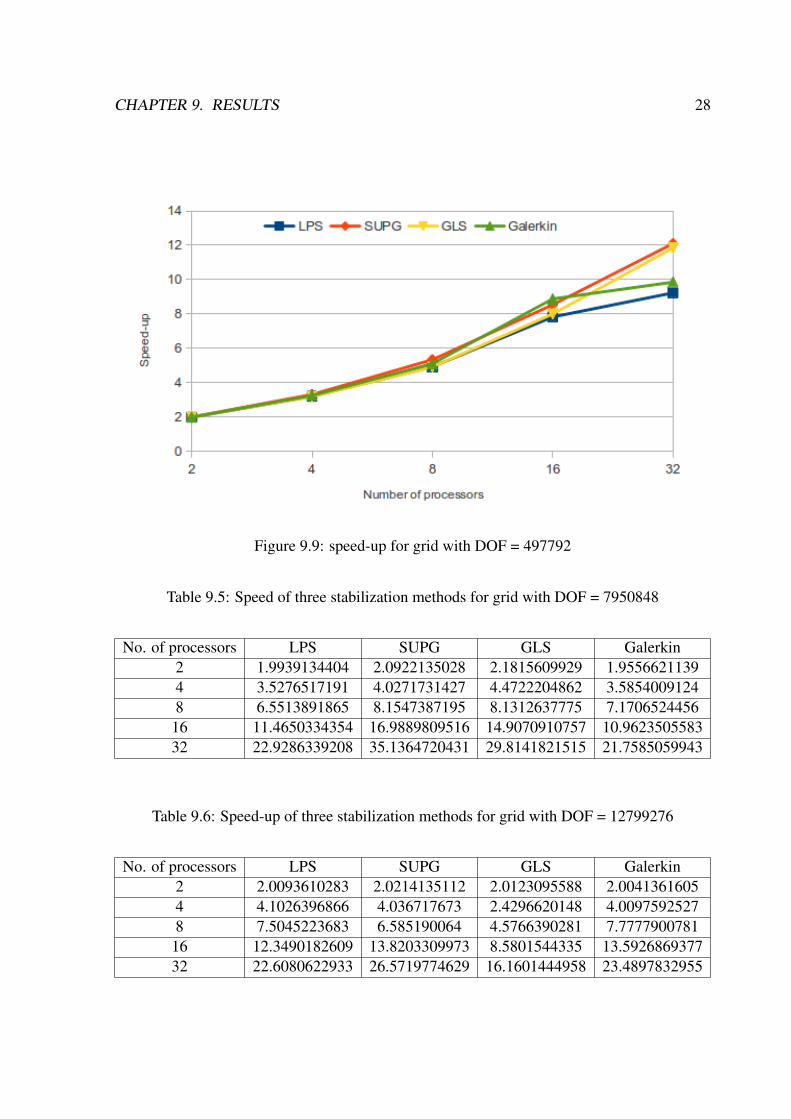
The figures 9.9,9.10 and 9.11 show that SUPG has higher speed-up as compared to other two

methods of stabilization. This suggests suitibility of SUPG for large parallel systems.

Table 9.4: Speed of three stabilization methods for grid with DOF = 497792

No. of processors LPS SUPG GLS Galerkin2 1.9958064861 2.0081818557 2.0139493968 2.00168693954 3.2113606599 3.3188351499 3.1932120085 3.2578008588 4.9337225295 5.3450905101 4.9206284223 5.1115204761

16 7.8301194368 8.539964943 8.0034959214 8.880354505232 9.2311236473 12.101164899 11.8489217498 9.8543914766

9.2.1 Conclusion

From the results we can conclude that LPS is suitable stabilization method when number of

processors is small and grid size is small. When the number of processors is large, SUPG is

more suitable.


Figure 9.9: speed-up for grid with DOF = 497792

Table 9.5: Speed of three stabilization methods for grid with DOF = 7950848


16 11.4650334354 16.9889809516 14.9070910757 10.962350558332 22.9286339208 35.1364720431 29.8141821515 21.7585059943

Table 9.6: Speed-up of three stabilization methods for grid with DOF = 12799276


16 12.3490182609 13.8203309973 8.5801544335 13.592686937732 22.6080622933 26.5719774629 16.1601444958 23.4897832955

Bibliography

[1] S. Ganesan and L. Tobiska,Stabilization by local projection for convection-diffusion and

incompressible flow problems,J. Sci. Comput.43, 3, 2010, 326–342

[2] T.J.R. Hughes and A.N. Brooks A multi-dimensional upwind scheme with no cross-wind

diffusion, Finite element methods for convection dominated flows, T.J.R. Hughes, 34,

ASME,New York,1979

[3] Finite element methods for the incompressible Navier- Stokes equations Ir. A. Segal J.M.

Burgerscentrum Re- search School for Fluid Mechanics

[4] Stabilized finite elen. nt r cthods for the velocity-pressure- stress formulation of incom-

pressible flows Marek A. Behr Leopoldo P. Franca Tayfun E. Tezduyar

[5] O. Axelsson and I. Kaporin. A posteriori error estimates in L2 -norm for the least-squares

finite element method applied to a first-order system of differential equations. Technical

Re- port 9945, Department of Mathematics, University of Nijmegen, The Netherlands,

1999

[6] MPI: The Complete Reference

[7] S. Ganesan, G. Matthies, L. Tobiska: Local projection stabilization of equal order interpo-

lation applied to the Stokes problem. Math. of Comput., (2008) 77, 2039-2060

30

e ciency of finite element stabilization schemes on parallel processors · e ciency of finite...

Documents