e. biondi, c. boldrini, a. passarella, m. conti - iit.cnr.it · 0 what you lose when you snooze:...
TRANSCRIPT

C
Consiglio Nazionale delle Ricerche
What you lose when you snooze: intercontact times and power-saving mode in opportunistic networks
E. Biondi, C. Boldrini, A. Passarella, M. Conti
IIT TR-12/2015
Technical Report
Settembre 2015
Iit
Istituto di Informatica e Telematica
0
What you lose when you snooze: intercontact times andpower-saving mode in opportunistic networks.
ELISABETTA BIONDI, CHIARA BOLDRINI, ANDREA PASSARELLA, and MARCOCONTI, IIT-CNR
In opportunistic networks, putting devices in energy saving mode is crucial to preserve their battery, andhence to increase the lifetime of the network and to foster user cooperation. However, a side effect of dutycycling is to reduce the number of usable contacts for delivering messages, thus increasing intercontacttimes and delays. In order to understand the effect of duty cycling in opportunistic networks, in this paperwe propose a general model for deriving the pairwise intercontact times when a duty cycling policy issuperimposed on the original encounter process determined only by node mobility. We consider both thecase of contacts with negligible duration and that of regular contacts. The model we propose is general, i.e.,not bound to a specific distribution of intercontact time. We validate the model in the case of exponentialand Pareto intercontact times, two popular assumptions in the related literature.
Categories and Subject Descriptors: C.2.2 [Computer-Communication Networks]: Network Protocols
General Terms: Design, Algorithms, Performance
Additional Key Words and Phrases: Wireless sensor networks, media access control, multi-channel, radiointerference, time synchronization
ACM Reference Format:
Elisabetta Biondi, Chiara Boldrini, Andrea Passarella, and Marco Conti. 2015. Duty Cycling in Opportunis-tic Networks: the Effect on Intercontact Times. ACM Trans. Model. Perform. Eval. Comput. Syst. 0, 0, Arti-cle 0 ( Wednesday 30th September, 2015), 39 pages.DOI:http://dx.doi.org/10.1145/0000000.0000000
1. INTRODUCTION
The widespread availability of smart, handheld devices like smartphones and tablethas stimulated the discussion and research about the possibility of extending the com-munication opportunities between users. Particularly appealing, towards this direc-tion, is the opportunistic networking paradigm (both as a standalone solution and insynergy with the infrastructure in mobile data offloading scenarios [Whitbeck et al.2012]), in which messages arrive to their final destination through consecutive pair-wise exchanges between users that are in radio contact with each other. Thus, usermobility, and especially user encounters, are the key enablers of opportunistic com-munications. Unfortunately, ad hoc communications tend to be very energy hungry[Friedman et al. 2013] and no user will be willing to participate in an opportunisticnetwork if they risk to see their battery drained in a few hours.
Energy issues in opportunistic networks have still to be fully addressed. In par-ticular, there are very few contributions that study how power saving mechanisms
This work was partially funded by the European Commission under the EINS (FP7-FIRE 288021), MOTO(FP7 317959), and EIT ICT Labs MOSES (Business Plan 2014) projects.Authors address: Via G. Moruzzi 1, 56124 Pisa, Italy; email: [email protected] to make digital or hard copies of part or all of this work for personal or classroom use is grantedwithout fee provided that copies are not made or distributed for profit or commercial advantage and thatcopies show this notice on the first page or initial screen of a display along with the full citation. Copyrightsfor components of this work owned by others than ACM must be honored. Abstracting with credit is per-mitted. To copy otherwise, to republish, to post on servers, to redistribute to lists, or to use any componentof this work in other works requires prior specific permission and/or a fee. Permissions may be requestedfrom Publications Dept., ACM, Inc., 2 Penn Plaza, Suite 701, New York, NY 10121-0701 USA, fax +1 (212)869-0481, or [email protected]© Wednesday 30th September, 2015 ACM 2376-3639/Wednesday 30th September, 2015/-ART0 $15.00DOI:http://dx.doi.org/10.1145/0000000.0000000
ACM Trans. Model. Perform. Eval. Comput. Syst., Vol. 0, No. 0, Article 0, Publication date: Wednesday 30th September, 2015.

0:2 E. Biondi et al.
impact on the amount of contacts that can be exploited to relay messages. With dutycycling, messages can be exchanged only when two nodes are in one-hop radio rangeand they’re both in the active state of the duty cycle. So, power saving effectively re-duces forwarding opportunities, because contacts are missed when at least one of thedevices is in a low-energy state that does not allow it to detect the contact. Since somecontacts are missed, the measured intercontact times, defined as the time intervalbetween two consecutive detected encounters between the same pair of nodes, is, ingeneral, larger and this clearly affects the delay experienced by messages. So far, thisaspect (i.e., the fact that duty cycling can affect the detected pairwise contacts) hasbeen largely ignored in the literature, despite the fact that all popular off-the-shelfwireless technologies (e.g., WiFi, Bluetooth) already implement some sort of periodiccontact probing.
The goal of this work is to understand how the exploitable mobility, i.e., the amountof contacts that can be used by node pairs for communicating, is modified by the dutycycling policy. To this aim, the contribution of this paper is twofold. First, we derive ananalytical model of the measured intercontact times between nodes after duty cyclingis factored in, i.e., by taking into account that some contacts may be missed. Whilederiving a closed-form characterisation of the detected intercontact times is in gen-eral too complex from an analytical standpoint (but we show that it is indeed possiblewhen intercontact times are exponential), this model can be used to compute numeri-cally their first two moments. As it is well-known, this is sufficient to approximate thedistribution of the detected intercontact times using hyper- or hypo- exponential dis-tributions, using standard techniques [Tijms and Wiley 2003]. Thus, with this model,we are able to obtain an approximated representation of intercontact times measuredwhen a duty cycling policy is in place under virtually any distribution.
2. PROBLEM STATEMENT
2.1. The duty cycling process
We use duty cycling in a general sense here, meaning any power saving mechanismthat hinders the possibility of a continuous scan of the devices in the neighbourhood.We assume that nodes alternate between the ON and OFF states. In the ON state,nodes are able to detect contacts with other devices. In the OFF state (which maycorrespond to a low-power state or simply to a state in which devices are switchedoff) contacts with other devices are missed. Using this generalisation, we are able toabstract from the specific wireless technology used for pairwise communications.
Duty cycling policies can be deterministic or stochastic, depending on how the lengthof their ON and OFF states is chosen (fixed, in the former case, varying according tosome known probability distribution in the latter). In the literature also non-stationaryduty cycling policies can be found, in which the length of ON and OFF states dependson some properties of the network (or a node’s neighborhood) at time t. For the sakeof tractability, we do not consider non-stationary duty cycling policies in this work.The model that we propose is able to capture the behaviour of both deterministic andstochastic duty cycling policies (for the latter, only the average behaviour is captured).We base our model on the deterministic duty cycling case (which requires a coarsesunchronisation between devices), then we later prove in Section 5 how this modelcaptures the average behaviour of the stochastic case (unsynchronised) as well.
In the following, we assume that the duty cycle process and the contact process areindependent and, considering a tagged node pair, we denote with τ the length of thetime interval in which both nodes are ON, and with T the period of the duty cycle.Thus, T − τ corresponds to the duration of the OFF interval and ∆ = τ
Tis the actual
duty cycle (i.e., the percentage of time nodes are in the ON state). In general, the ON
ACM Trans. Model. Perform. Eval. Comput. Syst., Vol. 0, No. 0, Article 0, Publication date: Wednesday 30th September, 2015.
Duty Cycling in Opportunistic Networks: the Effect on Intercontact Times 0:3
interval can start anywhere within T but here, without loss of generality, we takeas t = 0 its starting time (for convenience of notation, we count duty cycles startingfrom the first one in which a contact is detected). Hence, ON intervals will be of type[iT, τ + iT ), with i ≥ 0 and OFF intervals of type [τ + iT, (i + 1)T ), with i ≥ 0. In thefollowing, ON and OFF intervals will be denoted with ION and IOFF , respectively.Hence, the set of all ON (OFF) intervals is given by
⋃∞
n=0 IONn (
⋃∞
n=0 IOFFn ).
Focusing on a tagged node pair, we can represent how the duty cycle function evolveswith time as in Equation 1:
d(t) =
{
1 if t mod T ∈ [0, τ)0 otherwise.
(1)
When d(t) = 1, both nodes are ON, thus their contacts, if any, are detected. The oppositeholds when d(t) = 0. Basically, d(t) operates a bandpass filtering on the contact processbetween a pair of nodes.
In a recent work [Trifunovic et al. 2014], the authors, considering three technolo-gies for opportunistic communications (Bluetooth, WiFi Direct, WLAN-Opp), study thetrade-off between the frequency at which devices discover each other and energy con-sumption. They derive a threshold of 1/100s−1, beyond which energy consumption onsmartphones drastically increases, making the discovery process not energy efficient.
2.2. The contact process
We now focus on the contact process. Similarly to the related literature [Picu et al.2012; Boldrini et al. 2014], we assume that, from the mobility standpoint, node pairsare independent. When two nodes meet, they remain in contact for a certain time, thenthey separate for a while, than they come into contact again. In many real scenarios,contact duration is orders of magnitude smaller than the time between contacts (Ta-ble ??). In particular, contact duration is often smaller than the typical duty cycle T(which is, in general, larger than 100s). When this happens, contacts can be safelyapproximated as instantaneous. This approximation makes the model simpler, andeasier to manipulate, and it will be our initial assumption for the model in Section 3.Later on, in Section 4, we release this assumption and we discuss the impact of contactduration and how it changes the modelling.
When contact duration is negligible, the contact process of each pair can be describedas a renewal process [Cox et al. 1962]. Focusing on a tagged node pair, we denote thetime between the (i−1)-th and i-th contacts as Si. By definition of renewal process, theintercontact times Si for this pair of nodes are independent and identically distributed(while they can follow different distributions for different pairs), hence Si ∼ S, for all i.The time Xi at which the i-th contact occurs can be obtained as Xi =
∑i
j=1 Sj , ∀i ≥ 1.
When contact duration is not negligible, the contact process of each pair can be mod-elled as an alternating renewal process [Cox et al. 1962]. In this case, the node pair al-ternates between the CONTACT state in which the two nodes are in radio range, anda state in which they are not. The time interval between the beginning and the end ofthe i-th contact is denoted as Ci. The time interval between the end of a contact and thebeginning of the next one again corresponds to the intercontact time and it is denotedas Si. Hence, the alternating renewal process corresponds to the independent sequenceof independent random variables {Ci, Si}, with i ≥ 1. Exploiting this notation, we have
that the time Xi at which the i-th contact begins is∑i
j=1 Sj +∑i−1
j=1 Cj , ∀i ≥ 1, while
the time Yi at which it ends is given by∑i
j=1 Sj +∑i
j=1 Cj , ∀i ≥ 1.
ACM Trans. Model. Perform. Eval. Comput. Syst., Vol. 0, No. 0, Article 0, Publication date: Wednesday 30th September, 2015.
0:4 E. Biondi et al.
3. MEASURED INTERCONTACT TIMES WHEN CONTACT DURATION IS NEGLIGIBLE
We now discuss how the measured contact process depends on the contact processdescribed above, starting from the negligible contact duration case.
3.1. Preliminaries
Let us denote with Sj the time between the (j − 1)-th and the j-th detected contact
(corresponding to the j-th measured intercontact time) and assume that at time Xj−1
a contact has been detected, as shown in Figure 1. For convenience of notation, inFigure 1 and in the following, the sequence number of the duty cycling interval inwhich the i-th contact takes place is denote with ni, while the sequence number ofthe ON interval in which the j-th detected contact takes places is denoted with nj−1.
Then, the detected intercontact time Sj is the time from Xj−1 until the next detected
d(t) )))
ɶnj−1T ɶn
j−1T +τɶXj−1
ɶSj
ɶXj
ɶn TT ɶn T +τ t
S1
S2
S3
S4
Fig. 1. Contact process with duty cycling
contact at Xj , which can be obtained by adding up the intercontact times Si between
Xj−1 and the next detected contact. Denoting with Nj the random variable measuringthe number of intercontact times between the (j − 1)-th and the j-th detected contact
(e.g. in Figure 1, Nj = 4), we obtain Sj =∑Nj
i=1 Si, hence P(Sj = x) = P(∑k
i=1 Si =x|Nj = k)P(Nj = k). Recalling that Si are i.i.d. by definition, if Nj were i.i.d. for all jand independent of the inter-contact times Si occurred before the (j − 1)-th detected
contact, then also Sj would be i.i.d. and the detected contact process could be treatedas a renewal process. Unfortunately, this is not the case. In fact, after noticing that Nj
is equal to k only if the first k−1 contacts are missed and the k-th is detected, the PDFof Nj can be written as follows:
P(Nj = k) =
k−1∏
z=1
P
Xj−1 +
z∑
v=1
Sv 6∈
∞⋃
v=nj−1
IONv
P
Xj−1 +
k∑
v=1
Sv ∈
∞⋃
v=nj−1
IONv
,
(2)where the first k − 1 factors denote the joint probability that none of the first k − 1contacts fall into any ON interval (recall that
⋃∞
v=nj−1IONv is the set of all ON inter-
vals after the nj−1-th) and the k-th term gives instead the probability that the k-thcontact is detected. Equation 2 shows that the distribution of Nj is a function of ev-
erything that has happened before the nj−1-th contact. In fact, Xj−1 can be rewritten
as Xj−2 + Sj−1, where Xj−2 is the time at which the previous detected contact tookplace and is given by the sum of Nj−1 intercontact times. Hence Nj and Nj−1 are not
ACM Trans. Model. Perform. Eval. Comput. Syst., Vol. 0, No. 0, Article 0, Publication date: Wednesday 30th September, 2015.

Duty Cycling in Opportunistic Networks: the Effect on Intercontact Times 0:5
independent. Unfortunately, dealing with this type of non memoryless process wouldbe impractical. Thus, in the following lemma, we derive the condition under whichsuch independence can be assumed. Intuitively, this happens when the distribution ofS does not vary much inside an ON or OFF interval, and thus the exact time withinan interval when a contact happens can be approximated as uniformly distributed inthat interval, regardless of when the previous contact took place.
LEMMA 3.1. When fSivaries slowly 1 in intervals of length T , {Nj}j≥1 can be mod-
elled as i.i.d. (hence, Nj ∼ N ), and the displacement ZON of a detected contact withinan ON interval is approximately distributed as Unif(0, τ).
PROOF. Since nj−1 denotes the ON interval in which the (j − 1)-th detected contact
takes places, we can rewrite Xj−1 as nj−1T + ZONj−1, where we have denoted with ZON
j−1
the displacement of the detected contact within the ON interval. If we substitute thisexpression to Xj−1 in Equation 2, we obtain the following:
k−1∏
z=1
P
nj−1T + ZONj−1 +
z∑
v=1
Sv 6∈
∞⋃
v=nj−1
IONv
P
nj−1T + ZONj−1 +
k∑
v=1
Sv ∈
∞⋃
v=nj−1
IONv
=
=
k−1∏
z=1
P
(
ZONj−1 +
z∑
v=1
Sv 6∈
∞⋃
v=0
IONv
)
P
(
ZONj−1 +
k∑
v=1
Sv ∈
∞⋃
v=0
IONv
)
, (3)
where the last equality is obtained operating a shift of the index nj−1 of ON intervals(in other words, we start counting from the nj−1-th interval, which becomes [0, τ) inour shifted reference system). We now want to find under which conditions ZON
j−1 isindependent of the history of the contact process. Let us assume, without loss of gener-ality, that the previous contact (whether detected or not) took place at t∗ (which, afterthe shift, is negative). Then, ZON
j−1 is equivalent to t∗+S under the constraint that t∗+Sfalls into an ON interval (i.e. the contact is detected). This can be cast, applying theformulas for conditional probabilities, into the following:
P(ZONj−1 > z) = P(τ > t∗ + S > z|τ > t∗ + S > 0) =
P (τ − t∗ > S > z − t∗)
P (τ − t∗ > S > −t∗). (4)
It is easy to see that, when the PDF of S (which we denote as fS) is slowly varying inintervals of length T , the ratio in the previous equation corresponds to the ratio of theareas below the PDF. Thus, we obtain the following:
P(ZONj−1 > z) ∼
(τ − z) · fS(τ − t∗)
τ · fS(τ − t∗)=
(τ − z)
τ(5)
The above proves that whatever the time t∗ of the previous contact, if the PDF of Sis slowly varying in intervals of length T , then ZON
j−1 would be uniformly distributedand independent of the previous evolution of the contact process. This concludes theproof.
COROLLARY 3.2. It holds, under the same assumption in Lemma 3.1, that thedisplacement of a missed contact within its OFF interval is distributed as ZOFF ∼Unif(0, T − τ).
1In the context of this paper, a function f(x) varies slowly in a given interval if, for any x1, x2 belonging to
that interval, fS(x1)fS(x2)
∼ 1. We are not implying that the function is slowly varying in the sense of [ADDREF].
ACM Trans. Model. Perform. Eval. Comput. Syst., Vol. 0, No. 0, Article 0, Publication date: Wednesday 30th September, 2015.

0:6 E. Biondi et al.
When Lemma 3.1 holds true, the detected intercontact times are, at least approxi-mately, a renewal process. Thus, we can express S as a random sum of i.i.d. randomvariables, according to the following definition.
Definition 3.3. The detected intercontact time S can be obtained as S =∑N
i=1 Si,where N is the random variable describing the number of contacts needed to get onedetected.
Random sums of i.i.d. variables have some useful properties, which we will exploit inSection 3.3 in order to derive the first two moments of S. Please also note that Defini-tion 3.3 is general, i.e., holds for any type of continuous intercontact time distributionand for any type of duty cycling policy.
3.1.1. When can we apply Lemma 3.1?. Before concluding this section, we analyse inwhich cases the assumption in Lemma 3.1 about the slowly varying nature of fS is rea-sonable. To this aim, we consider two popular assumptions for the distribution of theintercontact times [Chaintreau et al. 2007; Gao and Cao 2011; Tournoux et al. 2011],namely the exponential and Pareto distributions. Let us start with exponentially dis-tributed intercontact times, whose rate we denote with λ. The PDF fS(x) = λe−λx ofthe intercontact time S is thus a positive, strictly decreasing convex function for x > 0.Hence, if we prove that fS(x) is slowly varying in the first interval of length T , i.e. in[0, T ], we are sure that the same holds true also for the next intervals. For fS(x) to be
slowly varying in [0, T ], we need fS(0)fS(T ) ∼ 1, which is equivalent to 1
e−λT . Thus, when
condition λT ≪ 1 holds, Lemma 3.1 also holds.When intercontact times are Pareto, we have fS(x) = αbα
(b+x)α+1 . The PDF is strictly
decreasing and convex also in this case, so we can again focus on [0, T ]. We take the
ratio fS(0)fS(T ) and we get
(
b+Tb
)α+1, which is approximately equal to 1 when T ≪ b. Since
the rate of a random variable is the inverse of the expectation (which is in turn equal tob
α−1 , with α > 1, in the Pareto case), T ≪ b is equivalent to λTα−1 ≪ 1 (assuming α > 1,
which is a common finding in real mobility traces [Boldrini et al. 2015]). Comparingthe exponential and Pareto cases, fixing the same contact rate λ for both distributions,when α > 2 the condition for fS to be slowly varying is easier to satisfy in the Paretocase than in the exponential case, since λT
α−1 < λT . The opposite holds true when1 < α < 2.
We can also study the Pareto with exponential cut-off distribution, suggestedin [Karagiannis et al. 2010] for intercontact times. As in [Clauset et al. 2009], we
define its PDF as x−αe−ξx ξ1−α
Γ(1−α,ξb) for all x ≥ b. In this case, it is difficult to find a
condition which is directly a function of the intercontact rate λ, because λ is equal toΓ(2−α,bξ)ξΓ(1−α,bλ) , thus we will derive the condition in terms of α, b, ξ, which are estimated
based on λ. Again, the PDF is strictly decreasing and convex, so we can study the firstinterval of length T in which the PDF is not zero, i.e. [b, b + T ]. Computing the ratio
fS(b)fS(b+T ) , we get
(
b+Tb
)α+1eξT . The two factors are exactly the same as those obtained
for the exponential and Pareto case. So, the condition here is T ≪ b ∧ ξT ≪ 1.We summarise the above results into Table I. Please note, however, that when these
conditions do not hold, Lemma 3.1 can still be used but instead of providing practicallyexact results, it will provide an approximation that will be as good as fS(x) is closeto being slowly varying in any intervals of length T . In Section 3.2.1 we will focus onsome practical cases in which the conditions hold and on some in which they don’t, andwe evaluate the error introduced exploiting Lemma 3.1 when fS is not slowly varyingin any interval of length T .
ACM Trans. Model. Perform. Eval. Comput. Syst., Vol. 0, No. 0, Article 0, Publication date: Wednesday 30th September, 2015.

Duty Cycling in Opportunistic Networks: the Effect on Intercontact Times 0:7
Table I. Conditions for fS to be slowly varying in intervals of length T
Exponential Pareto Pareto with exponential cut-off Lognormal
λT ≪ 1 λTα−1
≪ 1 T ≪ bλ ∧ ξλT ≪ 1
Table II. Table of notation - General
T , τ period of duty cycle and duration of the ON period
∆ fraction of time nodes are in ON
IONi i-th ON interval, corresponding to [iT, τ + iT )
IOFFi i-th OFF interval, corresponding to [τ + iT, (i+ 1)T )
fX(x), FX(x) PDF and CDF of random variable X
S intercontact time
S detected intercontact time
N number of intercontact times taking places before the next contact is detected
ZON , ZOFF displacement of a contact within its ON (OFF) interval
Xi time at which the i-th contact happens
Xi time at which the i-th detected contact happens
3.2. Deriving the distribution of N
Definition 3.3 tells us that the detected intercontact time S is a function of N and Si.In this section, we study the probability distribution of N , defined as the number ofcontacts needed, after a detected contact, in order to catch the next one.
Recall that we are assuming the detected contact process to be renewal, so we focuson the portion of this process between two detected contacts. Under the renewal as-sumption, we can focus, without loss of generality, on what happens between the firstand second detected contact. Then, the rationale behind the derivation of N is prettyintuitive. In fact, N = 1 corresponds to the case where the first intercontact time aftera detection ends in an ON interval. For case N = 2, the first intercontact ends in anOFF interval, while the following one ends in an ON interval after the point in timewhere the first intercontact time has finished. All other cases follow using the sameline of reasoning. Please recall that, in the following, ON and OFF intervals will be de-noted with ION and IOFF , respectively. Additional notation is summarised in Table II.
The derivation of the PMF of N in Theorem 3.4 below quantifies the probabilityP{N = k}. The line of reasoning for deriving this result is as follows. Let us definerandom variable Ek, which is equal to one when the k-th of these contacts is in an ONinterval, equal to zero otherwise. It is easy to see that the following holds true:
P (N = k)=P (E1 = 0, ..., Ek−1 = 0, Ek = 1) , (6)
i.e., the k-th contact is the first contact detected if it falls into an ON interval and allprevious ones fall in an OFF interval. Recalling that Xk denotes the time at which thek-th contact happens and that nk−1 is the index of the interval in which the previouscontact happened, it is easy to see that the following holds:
P(Ek = 0) =
∞∑
nk=nk−1+1
P(
Xk ∈ IOFFnk
)
(7)
P(Ek = 1) =
∞∑
nk=nk−1+1
P(
Xk ∈ IONnk
)
, (8)
ACM Trans. Model. Perform. Eval. Comput. Syst., Vol. 0, No. 0, Article 0, Publication date: Wednesday 30th September, 2015.
0:8 E. Biondi et al.
where we have derived the probabilities that the starting point Xk of the k-th con-tact is in any of the OFF (Equation 7) or ON (Equation 8) intervals after the one inwhich the previous contact has taken place. Quantity P
(
Xk ∈ IONnk
)
can be written ex-
plicitly as FXk(nkT + τ) − FXk
(nkT ), after recalling that IONnk
= [nkT, nkT + τ), while
P(
Xk ∈ IOFFnk
)
= FXk((nk + 1)T ) − FXk
(nkT + τ). [Ricordarsi che per k=1 e legger-mente diverso visto che puo accadere nello stesso ON del contatto zero. In pratica sipuo trascurare.] If we take into account the dependencies, i.e. the fact that one contactcan only start after the previous one, we can rewrite Equation 6 as:
∞∑
n1=n0+1
P(
Xi ∈ IOFFni
)
· · ·
∞∑
nk−1=nk−2+1
P(
Xi ∈ IOFFni
)
∞∑
nk=nk−1+1
P(
Xk ∈ IONnk
)
(9)
In [Biondi et al. 2014a] we have solved the above equation directly, but closed formsolutions could be obtained only for exponential intercontact times. In many practicalapplications, however, it is more convenient to have a closed form for P{N = k}, inorder to better capture its dependency on ∆ and on the original intercontact times. Forthis reason, below we derive a model that leads to an approximate closed form solutionof P{N = k} that is very accurate in a large set of mobility/duty cycling scenarios.
THEOREM 3.4 (PMF OF N). The probability mass function of N can be approxi-mated by the following:
{
P{N = 1} = g, k = 1P{N = k} = (1 − g)(1− p)k−2p, k ≥ 2
(10)
where g =∑∞
n1=11τ
∫ τ
0P(
z + S1 ∈ IONn1
)
dz, p =∑∞
n2=11
T−τ
∫ T−τ
0P(
τ + z + S2 ∈ IONn2
)
dz.2
PROOF. Let us start from case N = 1. The following equalities hold:
P{N = 1} = P{E1 = 1} =
∞∑
n1=n0+1
P(
X1 ∈ IONn1
)
=
∞∑
n1=n0+1
P
(
X0 + S1 ∈ IONn1
)
, (11)
where X0 as usual denotes the time at which the last contact has been detected. Ex-ploiting Lemma 3.1, we can rewrite X0 as n0T + ZON . Shifting everything by n0 andapplying the law of total probability, we obtain the following:
P{N = 1} =
∞∑
n1=1
P(
ZON + S1 ∈ IONn1
)
(12)
=
∞∑
n1=1
∫ τ
0
P(
z + S1 ∈ IONn1
)
P(ZON = z) (13)
=∞∑
n1=1
1
τ
∫ τ
0
P(
z + S1 ∈ IONn1
)
dz. (14)
For the sake of convenience, in the following we use g to indicate the latter expression.Let us now consider case N = 2, which means that the first contact is missed and
the second one is detected, i.e. P{N = 2} = P{E1 = 0, E2 = 1}. In this case, we have
2Equivalent expressions for g and p are g = 1τ
∑∞
n=0
∫ τ
0[FS(nT +τ−z)−FS(nT )+FS ((n+ 1)T + τ − z)−
FS ((n+ 1)T − z)]dz and p = 1T−τ
∑∞
n=0
∫ T−τ
0[FS ((n+ 1)T − z)− FS ((n+ 1)T − τ − z)].
ACM Trans. Model. Perform. Eval. Comput. Syst., Vol. 0, No. 0, Article 0, Publication date: Wednesday 30th September, 2015.

Duty Cycling in Opportunistic Networks: the Effect on Intercontact Times 0:9
the following:
P{N = 2} =
∞∑
n1=n0+1
P(
X1 ∈ IOFFn1
)
(
∞∑
n2=n1+1
P(
X2 ∈ IONn2
)
)
(15)
Exploiting the property of conditional probabilities, the second term at the right-handside of the above equation can be rewritten as follows:
∞∑
n2=n1+1
P(
X2 ∈ IONn2
)
=
∞∑
n2=n1+1
P(
X1 + S2 ∈ IONn2
|X1 ∈ IOFFn1
)
(16)
=∞∑
n2=n1+1
∫
IOFFn1
P(
t1 + S2 ∈ IONn2
)
P(X1 = t1|X1 ∈ IOFFn1
) (17)
=∞∑
n2=n1+1
∫ T−τ
0
P(
n1T + τ + z + S2 ∈ IONn2
)
P(ZOFF = z) (18)
=
∞∑
n2=1
∫ T−τ
0
P(
τ + z + S2 ∈ IONn2
)
P(ZOFF = z). (19)
In Equation 16 we have conditioned on the first contact falling into an OFF inter-val, which follows from the first term at the right-hand side of Equation 15. Then,we go from Equation 16 to Equation 17 applying the law of total probability. Note
that we stretch the notation here, and we use∫
IOFFn1
for denoting∫ τ+n1T
n1T. Finally, ap-
plying Corollary 3.2 we obtain Equation 18, which is then shifted by n1. Now, thesummation in n2 does not depend on what happens to the previous contacts andit is only a function of S2 and the duty cycling parameters τ and T . For the con-venience of notation, in the following we use p to synthetically denote probability∑∞
n2=11
T−τ
∫ T−τ
0P(
τ + z + S2 ∈ IONn2
)
dz.
Let us go back to the right-hand side of Equation 15. We have just derived the sec-ond term, now we have to study the first term
∑∞
n1=n0+1 P(
X1 ∈ IOFFn1
)
in order to
complete the analysis of P{N = 2}. Quantity∑∞
n1=n0+1 P(
X1 ∈ IOFFn1
)
corresponds tothe probability that the first contact does not fall into an ON interval, hence corre-sponds to 1− P{N = 1}, which is given by 1− g. Putting everything together, we havethat P{N = 2} = (1 − g)p.
For N = 3 the line of reasoning is similar. The only difference is that the sequence ofevents is now missed-missed-detected, i.e. P{N = 3} = P{E1 = 0, E2 = 0, E3 = 1}. Thiscorresponds to the following:
P{N = 3} =
∞∑
n1=n0+1
P(
X1 ∈ IOFFn1
)
[
∞∑
n2=n1+1
P(
X2 ∈ IOFFn2
)
(
∞∑
n3=n2+1
P(
X3 ∈ IONn3
)
)]
(20)Again, we want to make the three summations independent. It is easy to see that∑∞
n3=n2+1 P(
X3 ∈ IONn3
)
can be manipulated exactly as∑∞
n2=n1+1 P(
X2 ∈ IONn2
)
in thecase P{N = 2} (see Equation 16 and following), obtaining again p. As for the sec-ond summation, equality
∑∞
n2=n1+1 P(
X2 ∈ IOFFn2
)
=∑∞
n2=n1+1 1−P(
X2 ∈ IONn2
)
holds,which can be rewritten as 1− p. The first summation, which is now independent of theother two, is again equal to 1−P{N = 1} = 1−g, from which P{N = 3} = (1−g)(1−p)p.Generalising this result to the case N = k, we obtain Equation 10. Please note that wehave to separate the first contact from the others that follow because the first contact
ACM Trans. Model. Perform. Eval. Comput. Syst., Vol. 0, No. 0, Article 0, Publication date: Wednesday 30th September, 2015.
0:10 E. Biondi et al.
happens, by definition, after a detected contact (which takes place in IONn ), while all
others follow a missed contact (which happens in IOFFn ).
Starting from the distribution of N in Theorem 3.4, we can easily derive its firsttwo moments and its coefficient of variation, which will be later used to compute themoments of S.
COROLLARY 3.5 (MOMENTS OF N). The first two moments and the coefficient ofvariation of the approximate PMF of N are:
E[N ] =1− g + p
p(21)
E[N2] =−g(p+ 2) + p2 + p+ 2
p2(22)
cv2N =(1− g)(g − p+ 1)
(−g + p+ 1)2(23)
It is interesting to note that, under certain conditions g and p becomes approximatelyequal, from which follows that the distribution of N is approximately geometric in thiscase. The formal statement of this property and its proof is provided in the corollarybelow.
COROLLARY 3.6 (N AS GEOMETRIC R.V.). When fS is a slowly varying function inintervals of length T , it holds that g and p are both approximately equal to τ
T, hence the
distribution of N becomes approximately geometric with parameter τT
and its momentsand coefficient of variation become:
E[N ] =T
τ(24)
E[N2] =T (2T − τ)
τ2(25)
cv2N =T − τ
T(26)
PROOF. Let us consider g and p as defined in Theorem 3.4. Probability g dependson ZON , while probability p depends on ZOFF . We fix ZON = z1 and ZOFF = z2.Then, g and p correspond to the sum of the green and blue areas in Figure 2. Let usdenote with An and Bn the areas within the n-th duty cycling interval for g and p,respectively. When fS is slowly varying in intervals of length T , they can be rewrittenas An = fS(nT )(τ − z1) + fS(nT )z1 = τfS(nT ) and Bn = τfS(nT ), from which it followsthat An = Bn, and neither of them depends on z1 and z2. Thus, we can write g =p =
∑∞
n=0 τfS(nT ). Now let us define Cn has the whole area under fS(x) in the n-thduty cycling interval. It is straightforward to derive that Cn = TfS(nT ). Using the
expressions so far derived, the ratio∑
nτfS(nT )
∑nTfS(nT ) becomes equal to τ
T. By definition of
PDF,∑
n Cn ∼ 1, which implies that∑
n τfS(nT ) ∼τT
, from which g ∼ τT
follows.
Remark 3.7. Lemma 3.1 and Corollary 3.6 hold under the same assumption of fSbeing slowly varying in any intervals of length T and make explicit use of fS beingapproximately flat in duty cycling interval. Theorem 3.4 exploits the uniformity ofcontact displacement in the intervals in which they take place but then uses the ac-tual functional form of fS. For this reason, Corollary 3.6 holds under more restrictiveconditions than Theorem 3.4.
ACM Trans. Model. Perform. Eval. Comput. Syst., Vol. 0, No. 0, Article 0, Publication date: Wednesday 30th September, 2015.

Duty Cycling in Opportunistic Networks: the Effect on Intercontact Times 0:11
Τ-z1 T-z1 T+Τ-z1 2T-z1 2T+Τ-z1T-Τ-z2 T-z2 2T-Τ-z2 2T+z2T 2Tt @sD
0.005
0.010
0.015
0.020
PDF of S
Duty cycle shifted by z1
Duty cycle shifted by Τ+z2
Fig. 2. Probabilities g and p. [Rifare in Gnuplot]
3.2.1. Validation of P{N = k}. In this section we validate our approximation for thePMF of N against simulation results. We set T to 100s, which is found to be a goodtrade-off in [Trifunovic et al. 2014]. Then, we explore the parameter space assumingthat intercontact times are either exponential or Pareto distributed. Simulations areperformed drawing intercontact time samples from these distributions and filteringthem according to the reference duty cycling process (considering two cases, τ = 20 andτ = 80, corresponding to 20% and 80% duty cycling). The number of contacts filteredout between two detected contacts gives us one sample of N . When all samples for Nare collected, we use them to compute the empirical PMF, which is compared againstthe analytical predictions in Theorem 3.4 and Corollary 3.6.
We first consider the case of exponential intercontact times and we explore threevalues for the rate λ: 0.1, 0.01, and 0.001s−1. Based on the condition in Table I, weexpect the model to provide very good approximations in the third case (λT = 0.1 ≪ 1),decent approximations in the second case (λT = 1), and discrepancies in the first case(because λT > 1). This is exactly what we observe in Figure 3, except that the model ispretty close to simulation results also when λ = 0.1. Zooming in for case λ = 0.1, τ = 20,we notice that the model predicts a slower decay than what is actually observed insimulations. Vice versa, for the same λ value but τ = 80 model prediction goes to zerofaster.
For the Pareto case, the condition for fS to be slowly varying in any interval of lengthT is λT
α−1 ≪ 1 (see Table I). Again, we take λ = 0.01s−1 and T = 10s (and two different
values for τ ). Since the Pareto distribution is characterised by two parameters, herewe have an additional degree of freedom. So, for the purpose of validation, we have se-lected two α values for the Pareto, 1.01, which is right after the threshold α = 1 for the
ACM Trans. Model. Perform. Eval. Comput. Syst., Vol. 0, No. 0, Article 0, Publication date: Wednesday 30th September, 2015.

0:12 E. Biondi et al.
0
0.1
0.2
0.3
0.4
0.5
0.6
5 10 15 20 25 30
PM
F
N
sim - 0.1model - 0.1
sim - 0.01model - 0.01
sim - 0.001model - 0.001
geom
0
0.01
0.02
0.03
0.04
0.05
0.06
10 20 30 40 50 60
(a) τ = 20, T = 100
0
0.2
0.4
0.6
0.8
1
1 2 3 4 5 6 7 8 9 10
PM
F
N
sim - 0.1model - 0.1
sim - 0.01model - 0.01
sim - 0.001model - 0.001
geom
00.0050.01
0.0150.02
0.0250.03
0.0350.04
1 2 3 4 5 6 7 8 9 10
(b) τ = 80, T = 100
Fig. 3. PMF of N: predictions of the approximate model VS empirical distribution - Exponential
convergence of the expectation, and 2.01, right after the threshold α = 2 for the con-vergence of the variance. These are the two critical points of this distribution [Boldriniet al. 2015]. Once α is fixed, we have selected b values recalling that b
α−1 = 1λ= E[S].
When α = 1.01, condition λTα−1 ≪ 1 becomes 10 ≪ 1, which is clearly not true, while
when α = 2.01 we get 0.099 ≪ 1. Thus, we expect discrepancies between the modeland simulation results in the first case. In particular, when α = 1.01 we expect the ap-proximation in Theorem 3.4 to provide better results that Corollary 3.6. And, in fact,Figure 4 confirms our results. The only reason why the geometric model seems to per-form better when τ = 8 compared to case τ = 2 is that with Pareto(1.01, 1) the vastmajority of contacts are small, hence P{N = 1} tends to be quite high in general andwhen τ = 8 simply P{N = 1} is higher for the geometric model.
0
0.2
0.4
0.6
0.8
1
1 2 3 4 5 6 7 8 9 10 11 12 13 14 15
PM
F
N
sim - 1model - 1
sim - 10model - 10
sim - 100model - 100
geom
(a) α = 1.01, τ = 20, T = 100
0
0.2
0.4
0.6
0.8
1
1 2 3 4 5 6
PM
F
N
sim - 1model - 1
sim - 10model - 10
sim - 100model - 100
geom
(b) α = 1.01, τ = 80, T = 100
Fig. 4. PMF of N: predictions of the approximate model VS empirical distribution - Pareto
3.3. Detected intercontact times
Exploiting the results in the previous section, here we discuss how to compute the firstand second moment of the detected intercontact time S for a generic node pair A,B.
The relation between S and S is stated by Definition 3.3, i.e., S =∑N
i=1 Si. Thus, Sis a random sum of random variables, and we can exploit well-known properties tocompute its first and second moment.
ACM Trans. Model. Perform. Eval. Comput. Syst., Vol. 0, No. 0, Article 0, Publication date: Wednesday 30th September, 2015.

Duty Cycling in Opportunistic Networks: the Effect on Intercontact Times 0:13
PROPOSITION 3.8. The first and second moment of S are given by the following:
E[S] = E[N ]E[S] (27)
E[S2] = E[N2]E[S]2 + E[N ]E[S2]− E[N ]E[S]2 (28)
cv2S
=cv2SE[N ]
+ cv2N (29)
In the following we will use these formulas to get some general insights on the possi-ble behaviour of S depending on the distribution of S and the duty cycle ∆. Specifically,when intermeeting times are exponential, the following result holds.
LEMMA 3.9. When intercontact times Si are exponential with rate λ and conditionλT ≪ 1 holds, the detected intercontact times are again exponential but with rate λ∆.
PROOF. When λT ≪ 1 we can apply Corollary 3.6. Thus, recalling that E[S] = 1λ
and cv2S = 1, and substituting them into the equations in Proposition 3.8, we obtain
E[S] = 1λ∆ and cv2
S= 1, which corresponds to an exponentially distributed random
variable with rate λ∆. Please note we had already obtained this result in [Biondi et al.2014a] using a more complex model and derivation.
We repeated the analysis for the Pareto case, for which E[S] = bα−1 and cv2S = α
α−2 .
To compute the moments of S we have to assume α > 2, otherwise E[S2] would not con-verge. We also assume that λT
α−1 ≪ 1 holds, so that we are sure that our model providesa very close approximation and we can use Corollary 3.6. Under these assumptions,
cv2S= 2∆
(α−2) +1 = α−(2−2∆)α−2 . So we know that the detected intercontact times maintain
an hyper-exponential behaviour (which implies high variability) but S in this case doesnot conform to any well known distribution. The more general case in which g 6= p isstudied below.
Now, we want to make the analysis more general, in particular, we want to an-swer the following question: can duty cycling transform a hypo-exponential intercon-tact time into a hyper-exponential measured intercontact time, or vice versa? To thisaim, we focus on the squared coefficient of variation of S. Specifically, we know that
cv2S=
cv2S
E[N ] + cv2N , so, in order for S to show a hyper-exponential behaviour, quantitycv2
S
E[N ] + cv2N has to be greater than 1. If we rewrite this expression as a function of g and
p, we obtain the following:
cv2S > 1−2g
p+
2
1− g + p. (30)
In Figure ?? we plot the right-hand side of this inequality, and we split it in the twocases of cv2S ≥ 1 and 0 < cv2S ≤ 1. Let us first focus on the first case, correspond-ing to Figure ?? and define ξ(g, p) = 1 − 2g
p+ 2
1−g+p. We can see that when g > p, a
hyper-exponential cv2S will always be above the surface ξ(g, p), thus leading to a hyper-
exponential detected intercontact time S. When p > g, the squared coefficient of vari-ation of S depends on whether cv2S stays above or below the surface. When it staysbelow, we get the interesting case of a hypo-exponential detected intercontact time ob-tained starting from a hyper-exponential one. For cv2S > 3, only an hyper-exponential
behaviour for S is possible.Let us now focus on case 0 < cv2S ≤ 1, corresponding to Figure ??. When p > g,
the detected intercontact time can only be hypo-exponential. Vice versa, denoting with
ACM Trans. Model. Perform. Eval. Comput. Syst., Vol. 0, No. 0, Article 0, Publication date: Wednesday 30th September, 2015.

0:14 E. Biondi et al.
ω(g) = 32 (g − 1) + 1
2
√
9− 10g + g2 the function resulting from the intersection between
when ξ(g, p) and plane cv2S = 0, when p < ω(g), S will always be hyper-exponential.For the values in between, one has to evaluate whether cv2S stays above or below thesurface ξ(g, p).
A special case is when g = p, which we know happens under the conditions of Corol-lary 3.6. Under this condition, the squared coefficient of variation of S inherits theproperties of that of S: if S is hyper-exponential then S is hyper-exponential, and viceversa (Figures ??-??).
We summarise all the regions derived above in Table III.
Table III. Summary of hypoexponential/hyperexponential regions depending oncv2S , g, p
cv2S≤ 1 cv2
S> 1
cv2S> 3 - always
1 < cv2S<= 3
p > g ∧ cv2S≥ ξ(g, p) g > p
p > g ∧ cv2S< ξ(g, p)
0 < cv2S <= 1p > g p < ω(g)
g > p > ω(g) ∧ cv2S ≤ ξ(g, p) g > p > ω(g) ∧ cv2S > ξ(g, p)
3.3.1. Tail behavior and convergence issues. We have discussed above that when intercon-tact times are Pareto, detected intercontact times do not feature one of the well knowndistributions. However, sometimes, it might be useful to be able to characterise conve-niently at least the tail of the distribution, which is very important when dealing withpotentially high variance distributions. To this aim, we provide the following result.
LEMMA 3.10. When intercontact times are Pareto with exponent α, the CCDF of Sdecays as a Pareto random variable with exponent α.
PROOF. Since S =∑N
i=1 Si, we can write the following:
P(S > x) =
∞∑
k=1
P{N = k}P(S1 + · · ·+ Sk > x). (31)
It has been shown [Ramsay 2006] that, when Si are i.i.d. Pareto random variables,P(S1 + · · · + Sk > x) goes as L(x)k
(
bx
)αwhen x → ∞, where L(x) is a slowly varying
function at x. Using this relationship, we can rewrite the above equality as:
P(S > x) ∼ L(x)
(
b
x
)α ∞∑
k=1
kP{N = k} (32)
∼ L(x)
(
b
x
)α
E[N ] (33)
∼
(
b
x
)α
(34)
This result is important because it tells us that if there are convergence prob-lems [Boldrini et al. 2015] with Si, the same problems will apply also to the detectedintercontact times, since they decays as a Pareto with the same exponent.
ACM Trans. Model. Perform. Eval. Comput. Syst., Vol. 0, No. 0, Article 0, Publication date: Wednesday 30th September, 2015.
Duty Cycling in Opportunistic Networks: the Effect on Intercontact Times 0:15
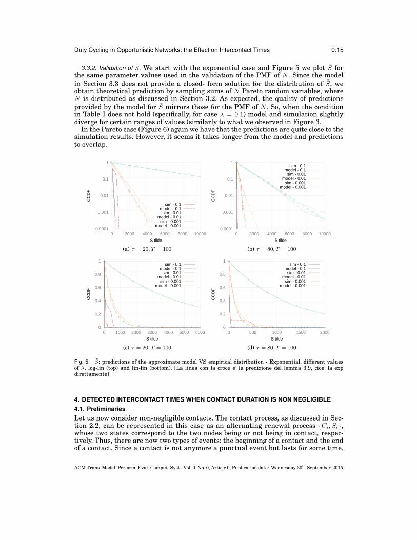
3.3.2. Validation of S. We start with the exponential case and Figure 5 we plot S forthe same parameter values used in the validation of the PMF of N . Since the modelin Section 3.3 does not provide a closed- form solution for the distribution of S, weobtain theoretical prediction by sampling sums of N Pareto random variables, whereN is distributed as discussed in Section 3.2. As expected, the quality of predictionsprovided by the model for S mirrors those for the PMF of N . So, when the conditionin Table I does not hold (specifically, for case λ = 0.1) model and simulation slightlydiverge for certain ranges of values (similarly to what we observed in Figure 3.
In the Pareto case (Figure 6) again we have that the predictions are quite close to thesimulation results. However, it seems it takes longer from the model and predictionsto overlap.
0.0001
0.001
0.01
0.1
1
0 2000 4000 6000 8000 10000
CC
DF
S tilde
sim - 0.1model - 0.1
sim - 0.01model - 0.01
sim - 0.001model - 0.001
(a) τ = 20, T = 100
0.0001
0.001
0.01
0.1
1
0 2000 4000 6000 8000 10000
CC
DF
S tilde
sim - 0.1model - 0.1
sim - 0.01model - 0.01
sim - 0.001model - 0.001
(b) τ = 80, T = 100
0
0.2
0.4
0.6
0.8
1
0 1000 2000 3000 4000 5000 6000
CC
DF
S tilde
sim - 0.1model - 0.1
sim - 0.01model - 0.01
sim - 0.001model - 0.001
(c) τ = 20, T = 100
0
0.2
0.4
0.6
0.8
1
0 500 1000 1500 2000
CC
DF
S tilde
sim - 0.1model - 0.1
sim - 0.01model - 0.01
sim - 0.001model - 0.001
(d) τ = 80, T = 100
Fig. 5. S: predictions of the approximate model VS empirical distribution - Exponential, different valuesof λ, log-lin (top) and lin-lin (bottom). [La linea con la croce e’ la predizione del lemma 3.9, cioe’ la expdirettamente]
4. DETECTED INTERCONTACT TIMES WHEN CONTACT DURATION IS NON NEGLIGIBLE
4.1. Preliminaries
Let us now consider non-negligible contacts. The contact process, as discussed in Sec-tion 2.2, can be represented in this case as an alternating renewal process {Ci, Si},whose two states correspond to the two nodes being or not being in contact, respec-tively. Thus, there are now two types of events: the beginning of a contact and the endof a contact. Since a contact is not anymore a punctual event but lasts for some time,
ACM Trans. Model. Perform. Eval. Comput. Syst., Vol. 0, No. 0, Article 0, Publication date: Wednesday 30th September, 2015.

0:16 E. Biondi et al.
0.0001
0.001
0.01
0.1
1
0.0001 0.01 1 100 10000 1e+06
CC
DF
S tilde
sim - 1model - 1
sim - 10model - 10
sim - 100model - 100
(a) τ = 20, T = 100
0.0001
0.001
0.01
0.1
1
0.0001 0.01 1 100 10000 1e+06
CC
DF
S tilde
sim - 1model - 1
sim - 10model - 10
sim - 100model - 100
(b) τ = 80, T = 100
0
0.2
0.4
0.6
0.8
1
0 1000 2000 3000 4000 5000 6000
CC
DF
S tilde
sim - 1model - 1
sim - 10model - 10
sim - 100model - 100
(c) τ = 20, T = 100
0
0.2
0.4
0.6
0.8
1
0 500 1000 1500 2000
CC
DF
S tilde
sim - 1model - 1
sim - 10model - 10
sim - 100model - 100
(d) τ = 80, T = 100
Fig. 6. S: predictions of the approximate model VS empirical distribution - Pareto, different values of b
contacts are detected more easily when their duration is not negligible. In fact, alsocontacts starting in an OFF interval can be detected, as long as they last until thenext ON interval. Actually, a contact can cover also two or more ON intervals, and inthis case pseudo-intercontact times are introduced. In fact, long contacts are split intosmaller measured contacts separated by intervals of size T − τ in which no commu-nication is possible (because the two nodes, despite theoretically in each other’s radiorange, are in the OFF interval of their duty cycle).
In order to make the model tractable, similarly to what we have done in Section 3,we need to model the measured contact process as a renewal process, this time of typealternate-renewal (because the measured contact process has now two states, corre-sponding to the measured contact and measured intercontact time). We denote themeasured contact process as {Ci, Si}, which is alternate renewal if {Ci, Si} are inde-pendent sequences of i.i.d. random variables. Based on the discussion for the negligiblecontact case, it is clear that also in this case the measured contact process is not in gen-eral renewal since the probability that a contact overlaps or not with an ON intervaldepends on where the contact starts, and the time at which the contact starts dependson the sequence of the previous contact and intercontact events. However, using anargument similar to that in Lemma 3.1 it is possible to prove that also in this case wecan assume, approximately, the independence for {Ci, Si}, provided that the PDF ofboth Ci and Si are slowly varying in intervals of length T . We do not provide the proofhere (it would be a repetition of the same concepts in Lemma 3.1 applied to Xi and Yi)and we summarise this result in Lemma 4.1 below.
ACM Trans. Model. Perform. Eval. Comput. Syst., Vol. 0, No. 0, Article 0, Publication date: Wednesday 30th September, 2015.

Duty Cycling in Opportunistic Networks: the Effect on Intercontact Times 0:17
LEMMA 4.1. When fS and fC are slowly varying functions in intervals of length T ,the measured contact process can be approximated as an alternating renewal process
{Ci, Si} and the displacement of the beginning (end) of a contact within its ON (or OFF)interval can be approximated as uniformly distributed in that interval.
Exploiting the fact that the measured contact process is approximately renewal un-der the conditions in Lemma 4.1, we can again focus on what happens between twodetected contacts. Differently from the previous case with negligible duration, the de-tected contact corresponding to the measured contact can now start also in an OFFinterval. For this reason, operating the usual shift of index as we have done in theprevious section, the starting point of our analysis will be the interval [0, T ] in whichwe know a detected contact has taken place, where its OFF interval is [0, T − τ ] and itsON interval [T − τ, T ]. All following OFF (ON) intervals will be of type [(i− 1)T, iT − τ ]([iT − τ, iT ]) with i > 1. Based on Lemma 4.1, we also know that the displacementof the beginning of a contact in an ON interval is distributed as ZON while that of acontact in an OFF interval as ZOFF . Similarly, the end of a contact in ON and OFFintervals will be displaced as ZON and ZOFF , respectively. Given the distribution ofdisplacements, we can easily quantity the probability of a contact beginning (ending)in an ON intervals, and that of a contact beginning (ending) in an OFF interval, whichwe denote as pON
s , pONe , pOFF
s , pOFFe , respectively. In more detail, since start and end
points of contacts are uniformly distributed in the duty cycling interval in which theytake place, the probability of having an event in an ON or OFF interval depends onthe length of that interval with respect to the overall duty cycle interval. Thus, thefollowing holds:
{
pONs = pON
e = τT
pOFFs = pOFF
e = T−τT
. (35)
4.2. Measured contact times
We start our derivation from the measured contact times, which are defined as the timeintervals during which the two nodes are in contact and both in the ON state. Thus,measured contact times are given by the overlap between the CONTACT state of thecontact process and the ON state of the joint duty cycle. Detected contact times, by def-inition, overlap with at least one ON interval. Thus, a real contact Ci which starts andends in the same OFF interval can never be detected and it does not contribute to themeasured contacts. We denote these undetected contacts as Cmiss
i and we will discusstheir role in the measured intercontact time in the next section. For those contactsthat do contribute to the measured contact time, the overlap between the CONTACTstate of the contact process and the ON state of the joint duty cycle can happen in twoways: either the contact starts in an ON interval (with probability pON
s ) or it starts inan OFF interval and lasts until the next ON interval (the joint probability of these twoevents is pOFF
s ·P(
Ci + ZOFF > T − τ)
). In the latter case, we do not observe the samedistribution as that of Ci, since only contacts lasting until the next ON interval canbe considered. Given the above three combinations (missed contact, contact startingin an ON interval, and contact starting in an OFF interval but detected nevertheless),we can split Ci as follows:
Ci =
Ci pONs
Chiti pOFF
s · phit
Cmissi pOFF
s
(
1− phit)
, (36)
where pONs and pOFF
s are given in Equation 35, while phit = P(
Ci + ZOFF > T − τ)
.
The PDF of Chiti can be obtained as fChit
i(c) = P
(
Ci = c|Ci + ZOFF > T − τ)
with
ACM Trans. Model. Perform. Eval. Comput. Syst., Vol. 0, No. 0, Article 0, Publication date: Wednesday 30th September, 2015.
0:18 E. Biondi et al.
support in (T − τ − ZOFF ,∞)3, which is equivalent to∫ T−τ
01
T−τ
fC(c)1−FC(T−τ−z)dz
(with c ∈ (T − τ − z,∞)) after applying the law of total probability and therules for conditioning. Similarly, the PDF of Cmiss
i can be computed as fCmissi
(c) =
P(
Ci = c|Ci + ZOFF ≤ T − τ)
with support in (0, T − τ − ZOFF ,∞). Hence, when
c ∈ (0, T − τ − z), fCmissi
(c) =∫ T−τ
01
T−τ
fC(c)FC(T−τ−z)dz, otherwise it is equal to zero.
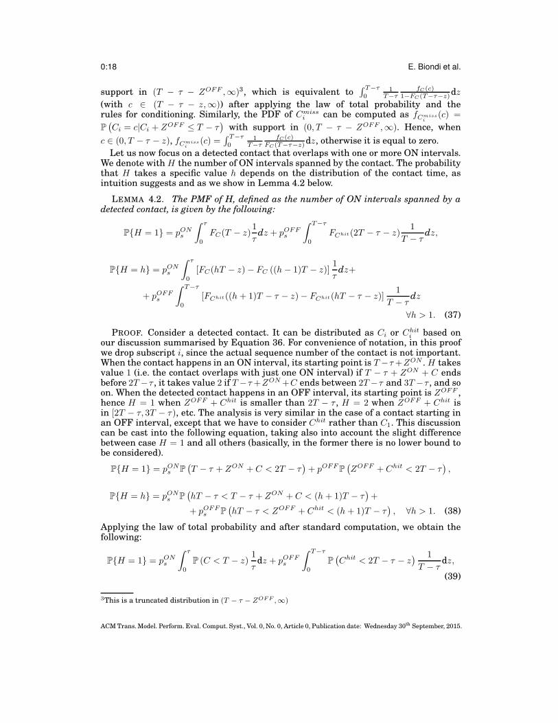
Let us now focus on a detected contact that overlaps with one or more ON intervals.We denote with H the number of ON intervals spanned by the contact. The probabilitythat H takes a specific value h depends on the distribution of the contact time, asintuition suggests and as we show in Lemma 4.2 below.
LEMMA 4.2. The PMF of H, defined as the number of ON intervals spanned by adetected contact, is given by the following:
P{H = 1} = pONs
∫ τ
0
FC(T − z)1
τdz + pOFF
s
∫ T−τ
0
FChit(2T − τ − z)1
T − τdz,
P{H = h} = pONs
∫ τ
0
[FC(hT − z)− FC ((h− 1)T − z)]1
τdz+
+ pOFFs
∫ T−τ
0
[FChit((h+ 1)T − τ − z)− FChit(hT − τ − z)]1
T − τdz
∀h > 1. (37)
PROOF. Consider a detected contact. It can be distributed as Ci or Chiti based on
our discussion summarised by Equation 36. For convenience of notation, in this proofwe drop subscript i, since the actual sequence number of the contact is not important.When the contact happens in an ON interval, its starting point is T −τ+ZON . H takesvalue 1 (i.e. the contact overlaps with just one ON interval) if T − τ + ZON + C endsbefore 2T −τ , it takes value 2 if T −τ+ZON +C ends between 2T −τ and 3T −τ , and soon. When the detected contact happens in an OFF interval, its starting point is ZOFF ,hence H = 1 when ZOFF + Chit is smaller than 2T − τ , H = 2 when ZOFF + Chit isin [2T − τ, 3T − τ), etc. The analysis is very similar in the case of a contact starting inan OFF interval, except that we have to consider Chit rather than C1. This discussioncan be cast into the following equation, taking also into account the slight differencebetween case H = 1 and all others (basically, in the former there is no lower bound tobe considered).
P{H = 1} = pONs P
(
T − τ + ZON + C < 2T − τ)
+ pOFFP(
ZOFF + Chit < 2T − τ)
,
P{H = h} = pONs P
(
hT − τ < T − τ + ZON + C < (h+ 1)T − τ)
+
+ pOFFs P
(
hT − τ < ZOFF + Chit < (h+ 1)T − τ)
, ∀h > 1. (38)
Applying the law of total probability and after standard computation, we obtain thefollowing:
P{H = 1} = pONs
∫ τ
0
P (C < T − z)1
τdz + pOFF
s
∫ T−τ
0
P(
Chit < 2T − τ − z) 1
T − τdz,
(39)
3This is a truncated distribution in (T − τ − ZOFF ,∞)
ACM Trans. Model. Perform. Eval. Comput. Syst., Vol. 0, No. 0, Article 0, Publication date: Wednesday 30th September, 2015.

Duty Cycling in Opportunistic Networks: the Effect on Intercontact Times 0:19
P{H = h} = pONs
∫ τ
0
P ((h− 1)T − z < C < hT − z)1
τdz+
+ pOFFs
∫ T−τ
0
P(
hT − τ − z < Chit < (h+ 1)T − τ − z) 1
T − τdz
∀h > 1. (40)
Finally, if we substitute the CDFs of C and Chit, we get Equation 37.
With the PMF of H in our hands, we can now derive the measured contact timein Lemma 4.3 below. Figures 7-8 show some possible instances of the problem whenH = 1 and H = 2, respectively. Note that each detected contact spanning H ON inter-vals introduces H samples of measured contact duration. In the following lemma, weinvestigate how these samples are characterised and how frequently they occur.
THEOREM 4.3 (MEASURED CONTACT DURATION). The measured contact time isapproximately given by the following:
C =
Cshort P (H=1)∑∞
h=1 hP (H=h)τ2
T 2
Cres P (H=1)( 2τ(T−τ)
T2 )∑
∞
h=1 hP (H=h) +P (H≥2)( 2τ
T )∑
∞
h=1 hP (H=h)
ZON P (H=1)( 2τ(T−τ)
T2 )∑
∞
h=1 hP (H=h) +P (H≥2)( 2τ
T )∑
∞
h=1 hP (H=h)
τP (H=1) (T−τ)2
T2∑∞
h=1 hP (H=h) +P (H≥2)( 2(T−τ)
T )+∑
∞
h=3(h−2)P (H=h)∑
∞
h=1 hP (H=h)
, (41)
where the PMF of H is given in Lemma 4.2 and the PDF of Cshort can be computed asfollows:
P{Cshort = c} =
{
1τ
∫ τ
0fC(c)
FC(τ−z)dz 0 < c < τ − z
0 otherwise. (42)
PROOF. When studying a measured contact, we first have to note that it cannot last,by definition, more than τ seconds, which is the maximum length of an uninterrupted(by an OFF interval) stretch of contact. In addition, consecutive measured contactsmay result from the same underlying contact that intersects with more than one ONinterval. The number of intersected ON intervals is given by H , derived in Lemma 4.2.The simplest case, which we study first, is when the contact overlaps with just one ONinterval of the duty cycle, case corresponding to H = 1. As illustrated in Figure 7, whenH = 1 there are four different cases depending on whether the contact starts in eitheran ON or OFF interval and whether it ends in either an ON or OFF interval. Recallthat pON
s = pONe = τ
Tand pOFF
s = pOFFe = T−τ
T). So, considering all possible cases,
when the contact is fully contained in the ON interval (Figure 7(a)), the measuredcontact duration is equal to the duration of Ci truncated in (0, τ − ZON ]. We denote itas Cshort, and its PDF is given in Equation 42. When the detected contact starts in anOFF interval and ends in the next OFF interval (Figure 7(b)), the measured contact isequal to τ (it lasts for the whole ON interval). When the detected contact starts in theON interval and ends in the OFF interval, the measured contact is equal to τ − ZON ,which is distributed as ZON (Figure 7(c)). Finally, if the detected contact starts in theOFF interval and ends in the ON interval, the measured contact lasts as long as ZON
(Figure 7(d)).When H = 2, the contact begins in [0, T ] and ends in [2T − τ, 3T − τ ] (see Figure 8).
Two separate detected contacts are introduced: one (totally or partially) overlapping
ACM Trans. Model. Perform. Eval. Comput. Syst., Vol. 0, No. 0, Article 0, Publication date: Wednesday 30th September, 2015.

0:20 E. Biondi et al.
d(t)!"# $
!"# $!"# $
!"# $! !
! !
d(t)
d(t)
d(t)
(a) (b)
(c) (d)
$"#%&'
%&'%&
()*+,-
Fig. 7. Case H = 1: types of overlapping.
with the first ON interval and one (totally or partially) overlapping with the secondON interval. When looking at the first one, in light of the discussion above, we knowthat it stops at T (because the devices go into energy saving mode) but it can starteither in [0, T − τ) (hence being detected as soon as the devices wake up at T − τ )or in [T − τ, T ) (hence being detected at T − τ + ZON ). Summarising, the length of ameasured contact in this case is τ with probability pOFF
s and ZON with probabilitypONs . Similarly, considering the second measured contact, we know that it starts being
detected at 2T − τ but it can stop either in the same ON interval or in the followingOFF interval, hence its length being equal to τ with pOFF
e or to ZON with probabilitypONe .
d(t)!"# !
d(t)
(a) (b)
(c) (d)
$!"# $!
)!"# ! $!"# $!
d(t)!"# !
d(t)$!"# $!
)!-# ! $!"# $!
#%"&'( &'(
#%"&'( &'(
Fig. 8. Case H = 2: types of overlapping.
The two cases found for H = 2 correspond to the two extreme cases that are alsopresent when H is greater than 2. The only difference is that, with H > 2 there aremany intermediate detected contacts equal to τ because the original contact completelyoverlap with the H−2 ON intervals between the first and the H-th one. Summarising,the detected contact can be equal to one of {τ, ZON , Cshort} with different probabili-ties. Weighting each case with the actual probability of occurrence we obtain Equa-tion 41.
ACM Trans. Model. Perform. Eval. Comput. Syst., Vol. 0, No. 0, Article 0, Publication date: Wednesday 30th September, 2015.

Duty Cycling in Opportunistic Networks: the Effect on Intercontact Times 0:21
With the above lemma we are able to fully characterise the detected contact dura-tion. In the next section, we study the detected intercontact times in order to completethe characterisation of the detected contact process.
4.3. The measured intercontact time
Measured intercontact times are defined as the time interval between two consecutivedetected contacts, which we have characterised above. Intuitively, they are a composi-tion of contact times (those that do not intersect any ON interval, which we have calledCmiss
i ) and intercontact times. Actually, there is another component, which only showsup when the real contact spans more than one ON intervals, which we will discusslater on. Hence, the expression for Si is much more complex than in the non negligi-ble contact case. In order to derive it, we start with the simplest case, focusing on asituation in which the last detected contact was a short contact (i.e., H = 1).
Table IV. Table of notation
Ci, Si Contact and intercontact timesCi, Si Detected contact and intercontact timesC∗
i Real contact that can be detectedCmiss
i Real contact that cannot be detectedCin Detected contact fully contained in an ON interval
Cshort Contact that intersects a single ON interval
A measured intercontact time starts when a measured contact time ends. The endof a measured contact can be the actual end point of its corresponding detected contact(if the latter ends in an ON interval) or otherwise to the end point of the ON interval(Figure 9). In the latter case, the portion of the detected contact between the end of the
d(t) )!"#"τ ! $!"#"τ $!
ZOFF
d(t) )!"#"τ ! $!"#"τ $!
S
Cmiss
S
ZOFF
S
Cmiss
S
Fig. 9. Short contact: two examples of measured intercontact time.
ON interval and the time at which the detected contact ends contributes to the mea-sured intercontact time. This quantity corresponds to the displacement of the endpointof the detected contact in the OFF interval, which is distributed as ZOFF according toLemma 4.1. A similar line of reasoning holds for the other extreme. In fact, a mea-sured intercontact time ends when a measured contact time starts. When the detectedcontact time corresponding to the measured contact time starts in an OFF interval,the time interval between the beginning of the detected contact and the beginning ofthe next ON interval contributes again to the measured intercontact time. Specifically,this time interval is again ZOFF long. These “residuals” of the contact (i.e. the partof detected contacts not overlapping with an ON interval) are only present depending
ACM Trans. Model. Perform. Eval. Comput. Syst., Vol. 0, No. 0, Article 0, Publication date: Wednesday 30th September, 2015.

0:22 E. Biondi et al.
on the ending (starting) point of the last (next) detected contact time. Recalling thatpOFFs = pOFF
e = T−τT
, these residuals can be modelled as R below:
R =
{
ZOFF with prob. T−τT
0 with prob. τT
(43)
Let us now focus on what happens between the two detected contacts. It is easy to seethat, regardless of when detected contact times starts and ends, the central part of themeasured intercontact time contains a certain number of intercontact times Si and ofmissed contacts Cmiss
i . If the next detected contact is the N -th real contact after the
last detected one, we have that Si is at least equal to∑N
i=1 Si +∑N
i=2 Cmissi , where the
PDF of Cmissi is P(Cmiss
i = c) = P(Ci = c|ZOFF + Ci < T − τ), as discussed before.When the last detected contact is long (H ≥ 2), it spans more than one ON inter-
val. However, from the standpoint of communication opportunities, the OFF intervalsbetween these ON intervals covered by the same contact cannot be used. Hence eachlong contact is split into smaller measured contacts separated by what we have calledpseudo-intercontact times, i.e. measured intercontacts of length T − τ , as shown in Fig-ure 10. So, while in the short contact case only one sample of measured intercontacttime corresponded to a single pair of detected contact, here a long contact introducesmultiple (specifically, H − 1) samples of intercontact times, all of size T − τ . What hap-pens after the end of the detected contact is exactly the same as what we discussedin the previous section: there will be a sequence of intercontact times Si and missedcontacts Cmiss
i , whose number depends on how many contacts are missed before the
next one is detected. This corresponds to formula R+∑N
i=1 Si+∑N
i=2 Cmissi +R, which
we have derived in the previous section.
d(t) )!"#"τ ! $!"#"τ $!
Rc
T-τ τ
%!"#"τ %!
d(t) )!"#"τ ! $!"#"τ $! %!"#"τ %!
T-τ RD
τ T-τ τ T-τ τ
&!"#"τ &!
Cmiss
S R
A S
RB
&!"#"τ &!
Cmiss
S S
RB
Fig. 10. Long contact: two examples of measured intercontact time.
Based on the above discussion, we know that measured intercontact times whencontact duration is non negligible can be either equal to T−τ (which is the contribution
of pseudo-intercontact times) or to R +∑N
i=1 Si +∑N
i=2 Cmissi + R, thus the following
lemma holds.
THEOREM 4.4 (MEASURED ICT). The measured intercontact time is approxi-mately given by the following:
S =
{
R+∑N
i=1 Si +∑N
i=2 Cmissi +R
∑∞
h=1 P (H=h)∑∞
h=1 hP (H=h)
T − τ∑
∞
h=2(h−1)P (H=h)∑∞
h=1 hP (H=h)
(44)
ACM Trans. Model. Perform. Eval. Comput. Syst., Vol. 0, No. 0, Article 0, Publication date: Wednesday 30th September, 2015.

Duty Cycling in Opportunistic Networks: the Effect on Intercontact Times 0:23
where R is defined in Equation 43.
PROOF. We have already explained how to derive the two components of the mix-ture distribution for S. The only missing part is the derivation of the probability withwhich each component is taken. Recall that there are two type of measured intercon-tact times: real ones and pseudo. One element of the first type is introduced any time ameasured contact ends. Instead, h elements of the second type are introduced by eachdetected contact spanning h ON intervals. From this, the above equation follows.
In order to obtain S the only missing piece is the distribution of N when contactduration is not negligible. Thus we derive it in the lemma below.
LEMMA 4.5 (PMF OF N). When contact duration is non negligible, the probabilitymass function of N can be approximated by the following:
{
P{N = 1} = g, k = 1P{N = k} = (1− g)(1− p)k−2p, k ≥ 2
(45)
where the expressions for g and p can be found in the body of the proof.
PROOF. When deriving the distribution of N , Equation 6 still holds also in the caseof non negligible contact duration. So, again, P(N = k) = P(E1 = 0, · · · , Ek−1 = 0, Ek =1), where Ek is zero if the k-th contact goes undetected, one otherwise. Again, note thatEk is dependent on the outcome of all previous events E1, · · · , Ek−1.
Let us start from the analysis of case N = 1, corresponding to the first contact beingdetected. For the sake of convenience, we focus on the complementary event, i.e., firstcontact not detected. This can happen only when the first contact starts in an OFFinterval and ends before the beginning of the next ON interval. Recalling that Xi andYi denote the start and end point, respectively, of the i-th contact, this is equivalent to:
P(N = 1) = 1−
∞∑
n1=2
P(
X1 ∈ IOFFn1
, Y1 ∈ IOFFn1
)
(46)
= 1−
∞∑
n1=2
P(
Z + S ∈ IOFFn1
)
P(
ZOFF + C < T − τ)
(47)
where the second equality follows after approximating (Lemma XXX) the displacementof start/end points of contacts as uniformly distributed in the intervals in which theytake place. In the following, we will denote the above quantity as g, similarly to thenon negligible contact case.
Now we move to N = 2, which implies that the first contact is not detected whilethe second one is. The probability of the first contact not being detected is equivalentto the complementary probability that we have derived above. The probability thatthe second contact is detected is similar to the probability of the first contact beingdetected with the difference that in this case we know for sure that the first contactwas fully contained in an OFF interval.
P(N = 2) =
∞∑
n1=2
P(
X1 ∈ IOFFn1
, Y1 ∈ IOFFn1
)
[
1−
∞∑
n2=n1+1
P(
X2 ∈ IOFFn2
, Y2 ∈ IOFFn2
)
]
(48)
= (1− g)
[
1−
∞∑
n2=2
P(
ZOFF + S ∈ IOFFn2
)
P(
ZOFF + C < T − τ)
]
(49)
Similarly to the negligible contact case, we denote the quantity in square bracketsabove as p.
ACM Trans. Model. Perform. Eval. Comput. Syst., Vol. 0, No. 0, Article 0, Publication date: Wednesday 30th September, 2015.

0:24 E. Biondi et al.
Let us now consider case N = 3, corresponding to the first two contacts missedand the third one detected. The probability that the first contact is missed has beencomputed above and it is given by 1 − g. The probability that the second contact ismissed is simply the complementary probability that the contact is detected, i.e. 1− p.Finally, applying Lemma XXX, it is easy to see that the probability of detecting thethird contact is again given by p. Generalising, we obtain the same expression for thePMF of N as in Theorem 3.4, with the difference that g and p are computed differentlyfrom g and p.
4.4. Validation
We now validate the results we have obtained for the measured contact (Theorem 4.3)and measured intercontact time (Theorem 4.4). Differently from Section 3.3.2, whereour main goal was to explore the solution space and to validate our approximation,here we focus on real contact datasets and we use it as a starting point for the valida-tion of our model. We focus on the PMTR and RollerNet traces (because of their smallduty cycling period, see Section 2.2), and for each user pair in these datasets we fitcontact and intercontact times to an exponential and Pareto distribution (for statisti-cal reliability, only pairs with more than 7 samples are considered ). Using MLE forfitting (specifically, the method discussed in [Clauset et al. 2009] for estimating bothscale and shape for the Pareto distribution) and the Cramer-von Mises test for evalu-ating the goodness of fit, we obtain the results summarised in Tables V-VI. Then, westudy separately the exponential and Pareto cases. Specifically, we focus on only thosepairs for which a given hypothesis (either exponential or Pareto) is not rejected, andwe apply our theoretical framework discussed in the previous section to representativeuse pairs (i.e. we configure the model using the MLE parameters of the selected pair).
Table V. Average rates (µ, λ) estimates from MLE fitting + outcome of Cramer-von Mises test.
type dataset included CvM Min. 1st Qu. Median Mean 3rd Qu. Max.
CT rollernet 43.95% 75.33% 0.01692 0.03979 0.04921 0.05229 0.06034 0.13850CT pmtr 40.06% 36.94% 0.0000714 0.005448 0.01253 0.01794 0.01873 0.4118ICT rollernet 84.88% 35.76% 0.0007926 0.001727 0.0025580 0.003082 0.00384 0.0184ICT pmtr 37.74% 4.76% 6.910e-06 1.132e-05 3.732e-05 5.017e-04 6.575e-04 3.127e-03
Table VI. Average parameters (α, b) estimates from MLE fitting + outcome ofCramer-von Mises test.
type dataset included CvM α b
CT rollernet 43.95% 98.79% 2.67 13.68CT pmtr 40.06% 99.21% 1.897 (2.471) 245.35 (588.37)ICT rollernet 84.88% 98.94% 1.91 120.71ICT pmtr 37.74% 97.48% 1.56 7991
4.4.1. The exponential case. We start with the PMTR trace. We consider the measuredcontact duration C first. Parameter µ, corresponding to the rate of the contact dura-tion, varies significantly across pairs in the PMTR trace, spanning several orders ofmagnitude (from 10−5 to 10−1). For this reason, in Figure 11 we plot simulation resultsagainst theoretical predictions for significant points of the µ distribution (correspond-ing to the minimum and maximum values, first and third quartiles, median and mean).The largest discrepancies appear for values of µ around 10−2 (both the mean/medianand third quartile of the µ distribution for PMTR fall in this range). For the RollerNettrace, the body of the distribution of µ is quite compact, and only the minimum and
ACM Trans. Model. Perform. Eval. Comput. Syst., Vol. 0, No. 0, Article 0, Publication date: Wednesday 30th September, 2015.

Duty Cycling in Opportunistic Networks: the Effect on Intercontact Times 0:25
maximum values are more distant. Thus, in this case we omit the plot for the medianand the first and third quartiles. In Figure 12 we observe a very similar behaviour tothe PMTR scenario.
Fig. 11. Measured contact duration when real contact and intercontact times are exponential (PMTR).
In order to clarify the reason for this behaviour, in Figure 13 we show, for a fixed T ,when H = 1 dominates the distribution of H . Recall that in Theorem 4.3 the mixtureprobabilities do not rely on the slowly varying assumption when H = 1. Thus, we ex-pect its predictions to be very accurate when either the probability of H being greaterthan 1 is negligible or when the slowly varying assumption holds. In Figure 13, we ob-serve that soon after µ = 10−2, H = 1 becomes the predominant component in the dis-tribution. However, around µ = 10−2 we are in a situation such that the dominance ofH = 1 has yet to kick in while at the same time the slowly varying approximation does
ACM Trans. Model. Perform. Eval. Comput. Syst., Vol. 0, No. 0, Article 0, Publication date: Wednesday 30th September, 2015.
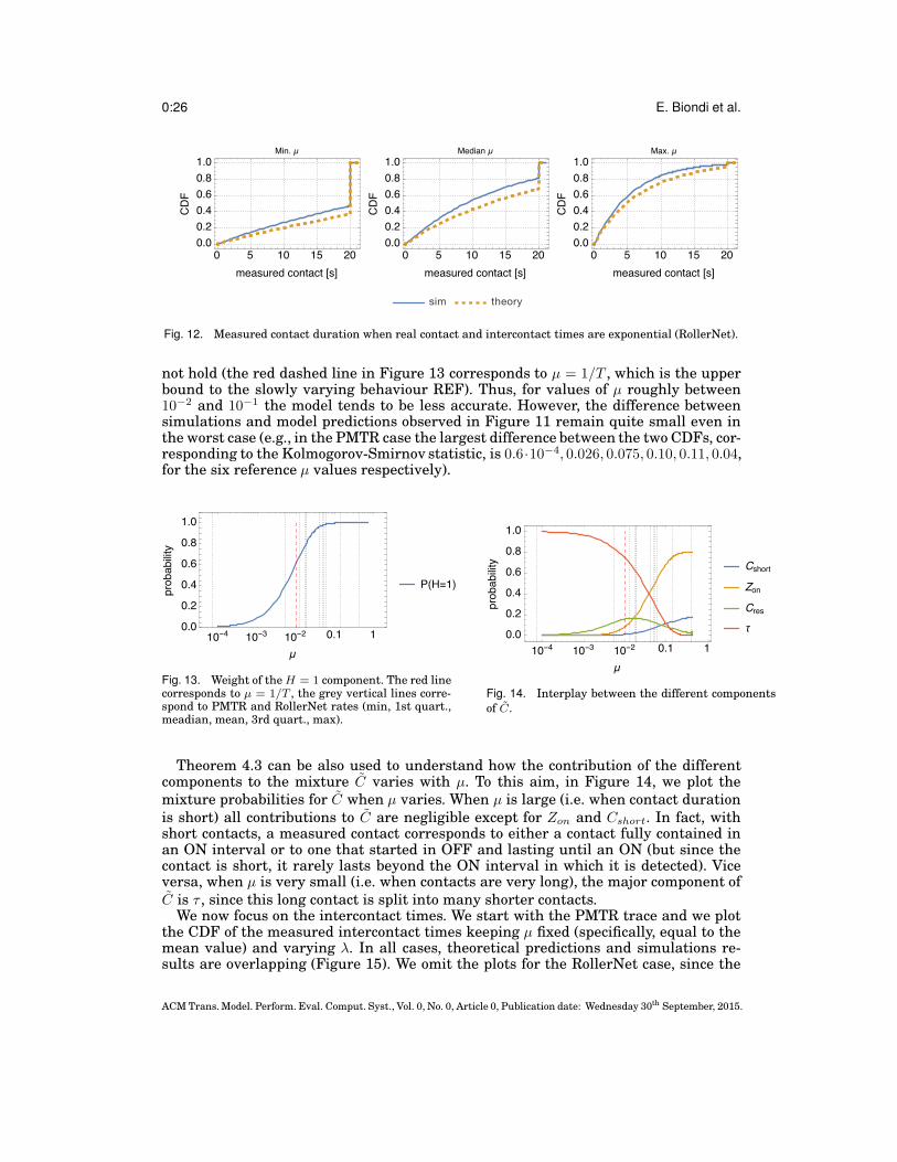
0:26 E. Biondi et al.
Fig. 12. Measured contact duration when real contact and intercontact times are exponential (RollerNet).
not hold (the red dashed line in Figure 13 corresponds to µ = 1/T , which is the upperbound to the slowly varying behaviour REF). Thus, for values of µ roughly between10−2 and 10−1 the model tends to be less accurate. However, the difference betweensimulations and model predictions observed in Figure 11 remain quite small even inthe worst case (e.g., in the PMTR case the largest difference between the two CDFs, cor-responding to the Kolmogorov-Smirnov statistic, is 0.6·10−4, 0.026, 0.075, 0.10, 0.11, 0.04,for the six reference µ values respectively).
Fig. 13. Weight of the H = 1 component. The red linecorresponds to µ = 1/T , the grey vertical lines corre-spond to PMTR and RollerNet rates (min, 1st quart.,meadian, mean, 3rd quart., max).
Fig. 14. Interplay between the different componentsof C.
Theorem 4.3 can be also used to understand how the contribution of the differentcomponents to the mixture C varies with µ. To this aim, in Figure 14, we plot themixture probabilities for C when µ varies. When µ is large (i.e. when contact durationis short) all contributions to C are negligible except for Zon and Cshort. In fact, withshort contacts, a measured contact corresponds to either a contact fully contained inan ON interval or to one that started in OFF and lasting until an ON (but since thecontact is short, it rarely lasts beyond the ON interval in which it is detected). Viceversa, when µ is very small (i.e. when contacts are very long), the major component ofC is τ , since this long contact is split into many shorter contacts.
We now focus on the intercontact times. We start with the PMTR trace and we plotthe CDF of the measured intercontact times keeping µ fixed (specifically, equal to themean value) and varying λ. In all cases, theoretical predictions and simulations re-sults are overlapping (Figure 15). We omit the plots for the RollerNet case, since the
ACM Trans. Model. Perform. Eval. Comput. Syst., Vol. 0, No. 0, Article 0, Publication date: Wednesday 30th September, 2015.

Duty Cycling in Opportunistic Networks: the Effect on Intercontact Times 0:27
same considerations apply and theoretical predictions remain virtually indistinguish-able with respect to simulation results. We expected this good result, since λ valuesare rather small (and, in all case but one, smaller than 1/T , which is the threshold forthe slowly varying conditions to hold true). It is also interesting to observe how thepresence of pseudo-intercontact times depends on µ. As shown in Figure 16, pseudo-intercontact times start appearing for µ values smaller than 0.06. In this range, longcontacts are split into many shorter contact and intercontact times.
Fig. 15. Measured intercontact duration when real contact and intercontact times are exponential (PMTR)- fixed µ.
4.4.2. The Pareto case. We now perform a similar analysis for those pairs for which thePareto hypothesis for contact and intercontact times was not rejected by the Cramer-von Mises test (more than 97% of pairs overall, see Table VI). Before delving into the
ACM Trans. Model. Perform. Eval. Comput. Syst., Vol. 0, No. 0, Article 0, Publication date: Wednesday 30th September, 2015.

0:28 E. Biondi et al.
Fig. 16. Probability of observing pseudo-intercontact times in S.
results for the PMTR and RollerNet traces, we start off with a general analysis of thedependence of C on the Pareto parameters α and b, similarly to what we have done inFigures 13 and 14. to this aim, we first need to make sure that H in the Pareto casedoes not suffer from the convergence problems that afflict heavy-tailed distributionfor small values of their exponent. Based on Lemma 4.2, it is easy to show that theCCDF of H decays as 1
xα , hence its expectation does not converge [Boldrini et al. 2015]for values of α smaller than 1. Similarly to what happens with the delay, the nonnegligible presence of arbitrarily large intercontact times steers the network towardsa degenerate behavior. However, in our two reference datasets, all parameters α aregreater than 1, so convergence problems do not show up in our case.
Next, we consider the predominance of the different components of H . When H ≥2, our model relies on the slowly varying approximation for the contact distribution,hence it may introduce errors when the slowly varying hypothesis does not hold. InFigure 17 we plot how P (H = 1) varies as a function of α and b. We observe thatthe only region in which the theoretical predictions are expected to be less accuratecorresponds to the bottom left one. In fact, for b ≫ T the slowly varying property holds,hence accuracy is guaranteed. When b < T , the model is expected to predict accuratelywhen P (H = 1) is high, which is generally true for α > 2 according to Figure 17.
Fig. 17. How P (H = 1) varies as a function of α, b.
METTERE PLOT DELLE COMPONENTI DI C AL VARIARE DI ALPHA E UNOAL VARIARE DI BETA. POI METTERE I SOLI GRAFICI BASATI SULLE TRACCE
ACM Trans. Model. Perform. Eval. Comput. Syst., Vol. 0, No. 0, Article 0, Publication date: Wednesday 30th September, 2015.

Duty Cycling in Opportunistic Networks: the Effect on Intercontact Times 0:29
We now analyse the interplay between the different components of C as we vary αand b.
Fig. 18. Interplay between the different components of C.
(a) Varying α (b set to the mean b = 245.40 in the dataset).
(b) Varying b (α set to the mean α = 1.898 in the dataset).
Fig. 19. Measured contact duration when real contact and intercontact times are Pareto (PMTR).
5. FROM DETERMINISTIC TO STOCHASTIC DUTY CYCLING POLICIES
In this section we show that the fixed duty cycling model provides a good approxima-tion also for non deterministic duty cycling. To this aim, we assume that individualduty cycles alternate between OFF and ON intervals whose lengths are both expo-nentially distributed with rate α and β, respectively. Exponentially distributed dutycycles are convenient to manipulate with Markov chains but the same results can be
ACM Trans. Model. Perform. Eval. Comput. Syst., Vol. 0, No. 0, Article 0, Publication date: Wednesday 30th September, 2015.

0:30 E. Biondi et al.
(a) Varying α (b set to the mean b = 13.68 in the dataset).
(b) Varying b (α set to the mean α = 2.667 in the dataset).
Fig. 20. Measured contact duration when real contact and intercontact times are Pareto (RollerNet).
Fig. 21. Probability of pseudo intercontact times as a function of α, b.
easily extended to non exponential duty cycles using semi-Markov chains. Due to spacelimitation, we will only go through the exponential case here.
The first step in the analysis involves the derivation of the joint duty cycling (whichis in the ON state when both nodes are ON, in the OFF state otherwise). Specifically,we investigate what is the probability distribution of the ON and OFF intervals in thejoint duty cycle. To this aim, we model the states of our system using a ContinuousTime Markov Chain (CTMC) with three states, like the one in Figure XXX. In state (1)
ACM Trans. Model. Perform. Eval. Comput. Syst., Vol. 0, No. 0, Article 0, Publication date: Wednesday 30th September, 2015.
Duty Cycling in Opportunistic Networks: the Effect on Intercontact Times 0:31
both nodes are ON, in state (2) either node is ON, in state (3) both nodes are OFF. Thetransition rate matrix and the jump matrix for the chain are provided below.
Q =
(
−2β 2β 0α −(α+ β) β0 2α −2α
)
(50)
J =
0 1 0α
α+β0 β
α+β
0 1 0
(51)
Thus, the sojourn time in the ON state follows an exponential distribution with rate2β and it corresponds to the length of the ON interval in the joint duty cycle. Instead,the OFF interval of the joint duty cycle corresponds to the time spent in the classcomposed of states (2) and (3). This time interval corresponds to the time at which thechain leaves state (1) until it moves back in. Since the chain moves mandatorily fromstate (1) to state (2), the time in OFF for the joint duty cycle corresponds to the hittingtime from (2) to (1), which can be obtained solving the following system of equations:
D2 =
{
T21 with probability p21T23 +D3 with probability p23
(52)
D3 = T32 +D2 (53)
in which we denote with D2 (D3) the time it takes to move from state (2) (from state(3)) to state (1), and with Tij the time it takes for a direct transition from state i tostate j. From CTMC properties, we know that Tij are exponential and their rates aregiven by the corresponding entry of matrix Q. By solving Equation 52 for the first andsecond moments we get the following:
E[D2] =2α+ β
2α2(54)
E[D22 ] =
10α3 + 11α2β + 6αβ2 + β3
2α4(α+ β)(55)
from which we can compute the squared coefficient of variation:
cv2 =2α(
6α2 + 3αβ + β2)
(α+ β)(2α + β)2+ 1 (56)
We assume that both α and β are strictly greater than zero4. For β approachingzero, the squared coefficient of variation approaches 4. For α approaching zero, cv2
approaches 1. Hence, we can conclude that D2 has, in general, a hyperexponentialbehaviour, which reduces approximately to an exponential behavior when α is muchsmaller than β.
The fixed duty cycling analysed in Sec. XXX can be considered as an approximationof the duty cycle studied in this section. In fact, the fixed duty cycling represents theaverage behavior of the above CTMC. Hence, the prediction about the detected inter-contact times in the fixed case are expected to provide a good approximation of the de-tected intercontact times with exponential duty cycling. Figure 22 validate this state-ment by comparing simulation results obtained with exponential duty cycling against
4When equal to zero we have the two extreme cases of nodes either always ON or always OFF. In the firstcase, there is no need to study the effect of duty cycling, in the second case nodes are never able to detecteach other.
ACM Trans. Model. Perform. Eval. Comput. Syst., Vol. 0, No. 0, Article 0, Publication date: Wednesday 30th September, 2015.

0:32 E. Biondi et al.
0
0.2
0.4
0.6
0.8
1
0 100000 200000 300000 400000 500000
CD
F
ICT [s]
Exp DC - SimFixed DC - Sim
Fixed DC - Theo
Fig. 22. Detected intercontact time with stochastic duty cycles.
the prediction obtained assuming the duty cycling is deterministic. Specifically, con-sidering a τ = 10s and T = 300s for the joint duty cycling (as in XXX traces), we obtainfor individual duty cycling β = 0.05 and α = 0.01, with cv2 = 1.34 for the joint OFFintervals. Then, we consider exponential intercontact times and TO BE COMPLETED
The above result is very important, as it shows that the fixed duty cycling case(which would require synchronisation between devices) is actually a good approxima-tion also for unsynchronised case in which the duty cycling is stochastic.
6. RELATED WORK
The OFF interval of the duty cycle on mobile devices corresponds to a state in whichdevices (or at least their network interfaces) are turned off or to a low-power state inwhich nodes are not able to detect contacts with other devices. The low-power state de-pends on the physical technology implemented on the device. Ad hoc communicationsin opportunistic networks typically go through either the WiFi or Bluetooth interface.Bluetooth has two main modes (scanning and being discoverable) that can be opti-mised. The scanning phase is found to be the most energy hungry across differentstudies [Friedman et al. 2013; Cano et al. 2006], thus it is often advised to reduce thescanning frequency in order to save battery. The Bluetooth discoverable state is gen-erally considered energy cheap (as stated in [Trifunovic et al. 2014; Friedman et al.2013]) but keeping the phone in the discoverable state indefinitely in the long runincurs in a significant energy consumption as well. For WiFi in ad hoc mode, the en-ergy for being idle is comparable to the energy consumed for sending and receivingmessages [Friedman et al. 2013], hence turning off the network cards when possi-ble is the simplest yet the only viable approach for increasing battery lifetime5. Sincead hoc WiFi is typically not supported by the most popular smartphones [Trifunovicet al. 2011], two innovative WiFi-based ad hoc communications modes, namely, WiFiDirect [WiF ] and WLAN-Opp [Trifunovic et al. 2011], have been recently proposed toaddress the problems of ad hoc communications in off-the-shelf smartphones. Unfor-tunately, their energy consumption is still quite high. In particular, as far as neigh-bour discovery is concerned, Bluetooth is found two times more energy efficient thanWLAN-Opp and about five times more energy efficient than WiFi Direct [Trifunovicet al. 2014]. Also for WiFi Direct and WLAN-Opp, the configured scanning intervalheavily affects the energy consumption. Based on the above discussion, it is easy to
5For 802.11 cards used in infrastructure mode energy consumption in the idle state (previously compara-ble to that used in the transmitting/receiving state) has been drastically reduced by the introduction of thePower Saving Mode (PSM) [Friedman et al. 2013]. Unfortunately, PSM for ad hoc is typically not imple-mented in smartphones’ 802.11 interfaces.
ACM Trans. Model. Perform. Eval. Comput. Syst., Vol. 0, No. 0, Article 0, Publication date: Wednesday 30th September, 2015.

Duty Cycling in Opportunistic Networks: the Effect on Intercontact Times 0:33
see that a baseline power saving approach consists in periodically switching off net-work cards when using ad hoc WiFi and reducing the scanning frequency when usingBluetooth/WLAN-Opp/WiFi Direct. Indeed, different scanning frequencies have beenused in the Bluetooth-based trace collection experiments discussed in Section ??. Theduty cycling model presented in Section 2 is perfectly suitable to represent these ap-proaches.
Feeney and Nilsson [Feeney and Nilsson 2001] measured the energy consumptionof a IEEE 802.11 WaveLan card. The result is that the power needed for transmit-ting, receiving and being idle (i.e., just listening to the wireless medium) shows thesame order to magnitudine, while sleep power is significantly smaller. From this re-sult, one understands that the only way for saving significant energy is to turn off thewireless interface. Using Nokia N95 mobile phones, Balasubramanian et al. [Balasub-ramanian et al. 2009] studied the energy consumption of the WiFi network interfacefor i) scanning and associating to an access point, ii) transferring data. Their resultsshow that, for data item of size 5K, the scan&associate energy is nearly five timesthe energy consumed for actually transferring the data. The authors also point outthat WiFi suffers from high maintenance energy overhead for keep the interface on.This result confirm that the most effective strategy for saving energy when using WiFiis to turn off the radio interface. Energy consumption of N95 phones in WiFi ad hocmode has been measured by Perrucci et al. [Perrucci et al. 2011]. Also in this case, thepower for transmitting, receiving, and being idle have been found of the same order ofmagnitude.
A recent work by Friedman et al. [Friedman et al. 2013] has questioned previousmeasurement results on the ground of two considerations. First, Friedman et al. pointout that the above previous studies were performed years ago and, given the rapid paceat which mobile devices are improved, their results may not be valid anymore. Second,in most previous measurement studies the performance of standalone interfaces inlab settings were considered, not exactly the same conditions in which they are allmounted on the same chip. And in fact the main results of [Friedman et al. 2013]are that Power Saving Mode on 802.11 cards is actually working quite well (this wasalready detected in [Perrucci et al. 2011]) and the previous claim [Feeney and Nilsson2001] that the power used for being idle was approximately the same as the powerneeded for tx/rx cannot be considered valid anymore. Unfortunately, this considerationholds only for 802.11 cards working in infrastructure mode. In fact, as shown in both[Friedman et al. 2013] and [Perrucci et al. 2011], the ad hoc mode is highly inefficientand PSM for ad hoc is typically not implemented in smartphone 802.11 interfaces.Thus, in the ad hoc case, it is still true that the energy for being idle is comparableto the energy consumed for sending and receiving messages, hence turning off thenetwork cards when possible is the simplest yet the only viable approach for increasingbattery lifetime.
Measurements of Bluetooth energy consumption are more consistent across pastand recent studies. When non communicating (i.e., when not sending/receiving pack-ets) Bluetooth can be in one of three states: scanning, when it searches for nearbyBluetooth devices, discoverable, when it can be detected by other scanning devices,nondiscoverable, when the Bluetooth interface is on but the device cannot be detectedby other scanning Bluetooth devices. The scanning phase is the more energy hungryacross different studies [Friedman et al. 2013; Cano et al. 2006] and for this reasonit is recommended to use it as little as possible. The effect of this choice, however, isthat user devices detect each other with some delay, thus reducing the opportunitiesfor communications. The Bluetooth discoverable state is generally considered energycheap (as stated in [Trifunovic et al. 2014], [Friedman et al. 2013]) but keeping the
ACM Trans. Model. Perform. Eval. Comput. Syst., Vol. 0, No. 0, Article 0, Publication date: Wednesday 30th September, 2015.

0:34 E. Biondi et al.
phone in the discoverable state indefinitely in the long run incurs in a significant en-ergy consumption.
All the above contributions were mostly focused on traditional mobile ad hoc com-munications, in which Bluetooth is used, e.g., for connecting the phone to a laptop orto wireless headphones (hence, the scanning phase is entered rarely, just to connect tothe desired device) and WiFi is in infrastructure mode. To the best of our knowledge,the only work focusing specifically on energy consumption in opportunistic networks,i.e., in which both Bluetooth and WiFi are used for pairwise communications betweenthe users of an ad hoc network, is that by Trifunovic et al. [Trifunovic et al. 2014].As far as WiFi is concerned, these authors focus on two innovative WiFi-based ad hoccommunications modes, namely, WiFi Direct [WiF ] and WLAN-Opp [Trifunovic et al.2011]. WiFi Direct has gained a lot of attention since it has been natively introduced onAndroid 4.0+ operated smartphones. Before that, WiFI ad hoc mode was available inthe phone hardware but disabled in software, requiring unrooting the device in orderto use it and hence hindering a large scale diffusion of opportunistic mobile applica-tions. However, WiFI Direct was more intended as a WiFi-based Bluetooth replace-ment for connecting together, e.g., laptops, printers, and media devices, rather thanfor actual opportunistic communications. In addition, its availability on Android hasbeen discontinued since version 4.3. Instead of stalling the implementation of oppor-tunistic applications due to the lack of a suitable MAC layer technology natively sup-ported by most popular mobile OSes, Trifunovic et al. [Trifunovic et al. 2011] suggestedadapting traditional WiFi capabilities available on any off-the-shelf smartphone. Theidea of WLAN-Opp is that mobile devices switch temporarily in a AP state (usingthe tethering/hotspot setting of the mobile phone) and act as APs for nearby devices(nodes take turn being APs). In [Trifunovic et al. 2014] WiFi Direct and WLAN-Oppare compared against Bluetooth in terms of their energy consumption for discoveringneighbours (a key aspect in opportunistic networks, since new contacts are deliveryopportunities) and connection maintenance. As far as neighbor discovery is concerned,Bluetooth is found two times more energy efficient than WLAN-Opp and about fivetimes more energy efficient than WiFi Direct. As expected, the energy consumptionfor all three protocols heavily depends on the scanning interval, i.e., how often theyscan their neighbourhood for new devices. For scanning intervals smaller than ∼ 100s,the power consumption increases drastically. Looking at energy consumption at a finerdetail, we see that in Bluetooth discovery, the higher amount of energy is consumedduring the scanning phase, while the discoverable mode is relatively cheap. Instead,for WLAN-Opp both being discoverable (i.e., when the device acts as AP) and discover-ing are expensive operations. In WiFi Direct the situation from the energy standpointis worse, since for detecting each others both devices have to be scanning at the sametime. So, as discussed in [Trifunovic et al. 2014], it is more suited to situations in whichboth devices intentionally scan at the same time rather than for continuous discovery.After the neighbour discovery phase, with all three protocols, a host-client connectionis established for communication. Being energy consumption highly asymmetric (i.e.,the device acting as AP in WiFi mode or slaves in Bluetooth mode consume much moreenergy), the authors of [Trifunovic et al. 2014] suggest a contact-duration-aware swaprole algorithm in order to fairly distribute energy consumption between the communi-cating parties.
A taxonomy proposed by Jun et al. [Jun et al. 2005] for traditional MANETs classi-fies duty cycling policies into four categories. With the synchronous mechanisms (themost popular of which is 802.11 Power Saving Mode) nodes all wake up/go to sleep atthe same time. The drawback of this approach is that it requires a global synchroni-sation among nodes and a fully connected network[Jun et al. 2005]. In asynchronousstrategies, neighbouring nodes select their wake-up slot so that they overlap with one
ACM Trans. Model. Perform. Eval. Comput. Syst., Vol. 0, No. 0, Article 0, Publication date: Wednesday 30th September, 2015.

Duty Cycling in Opportunistic Networks: the Effect on Intercontact Times 0:35
another. In cell-base schemes the network is divided into non-overlapping cells, withinwhich only a few nodes are awake at a given time. In on demand strategies nodesare equipped with an additional low-power radio interface that is used for signallingwake up or sleep commands. Unfortunately, all the above strategies were designed fora dense and connected network, which is quite different from the typical conditions inwhich opportunistic networks operate.
Abstracting the specific communication technology used and building upon the ideathat neighbour discovery is an energy-expensive operation in general, the vast major-ity of papers dealing with power saving issues in opportunistic networks have focusedon the contact probing phase. As seen above, reducing and optimising the probingfrequency is equivalent to implementing a duty cycling policy in which nodes switchbetween low-power and high-power states, corresponding to OFF intervals (in whichcontacts are not detected) and ON intervals (in which contacts are detected), respec-tively. Contact probing schemes can be classified into fixed, when the ON/OFF dura-tion of the duty cycle is established at the beginning and never changed [Jun et al.2005], or adaptive, when the frequency of probing is increased or decreased accord-ing to some policy [Choi and Shen 2009]. Both fixed and adaptive strategies can becontext-oblivious [Jun et al. 2005], if they do not exploit information on user past be-haviour or position, or context-aware [Drula et al. 2007; Wang et al. 2009] otherwise.In order to address the lack of duty cycling mechanisms in sparse networks, [Jun et al.2005] proposes three schemes based on different availability of information at nodes.In the oracle case, nodes can predict their meetings, so they are able to wake up andget to sleep exactly at the beginning and end of a contact. This strategy is clearly usedfor benchmarking only, since real nodes are not omniscient. At the opposite range, theauthors identify the zero knowledge strategy, in which nodes have no means to esti-mate their future contacts, so basically enter a periodic, fixed, beaming period in whichneighbour discover is performed. Between these two extremes, the authors propose thepartial knowledge strategy, in which they assume that nodes are able to estimate themean and variance of the intercontact times and the contact times, information thatis used in order to predict when to scan more intensely for neighbours (intuitively, notright after a contact has ended).
The work by Choi et al. [Choi and Shen 2009] considers a DTN in which nodes wakeup at synchronised intervals and sends beacons in order to discover new neighbours.If no neighbour is discovered, the next beaconing period is set at double the previousinterval and nodes sleep until then. This exponential increasing is performed until amaximum value is reached. The main contribution of the paper lies in designing analgorithm (AEB) in order to compute this maximum value in order minimise powerconsumption and maximise the probability of detecting a contact. This is done exploit-ing the CDF of contact duration. Unfortunately, this algorithm is targeted at randommobility models (in which contact and intercontact times are i.i.d.), hence it is arguablewhether it is applicable to real networks.
An energy-efficient variation of Bluetooth discovery mode is proposed in [Drula et al.2007]. This work starts from the observation that wherever a neighbour is encoun-tered, other contacts are likely to happen as well. So the authors propose two schemes:one in which the discovery mode is triggered by indications of recent activities andone in which previous contacts at a specific location (access to a positioning system isassumed) are used to switch the device to a more aggressive scanning mode.
Wang et al. [Wang et al. 2009], assuming that nodes scan their surroundings ev-ery T and that contact duration for a pair of nodes is stationary and i.i.d. are able toprove that among all social-oblivious strategies with the same average contact probinginterval, the strategy exploiting fixed probing intervals is optimal for minimising theprobability of missing a contact. This is an interesting result, supporting the use of
ACM Trans. Model. Perform. Eval. Comput. Syst., Vol. 0, No. 0, Article 0, Publication date: Wednesday 30th September, 2015.

0:36 E. Biondi et al.
simple fixed contact probing strategies over more elaborate ones. Then, the authorspropose some heuristic social-aware adaptive probing algorithm, of which the STARalgorithm, which adapts to the contact arrival process exploiting a self-similar argu-ment, is shown to outperform the others.
The work in [Altman et al. 2013] is a theoretical work that extends the fluid model oftwo-hop forwarding with the fact that nodes, with a certain rate, go from the inactivestate to the active state (in which they start beaconing until they receive a messagecopy) and use this model to solve the optimal activation problem. The model is tailoredto a homogeneous environment (i.e., nodes with contact process i.i.d.) and, as discussedby the authors themselves, cannot be used as it is to describe the heterogeneous envi-ronments seen in real mobility traces. Moreover, the model is not directly applicableto duty-cycling-style power saving, since node activation is considered monotone, i.e.,once activated nodes remain active until their battery is depleted or the deadline isreached.
All the above contributions aimed at deriving a power saving strategy for DTNs, beit fixed [Jun et al. 2005] or adaptive [Choi and Shen 2009], social-oblivious [Jun et al.2005] or social-aware [Drula et al. 2007; Wang et al. 2009]. This is not our goal. iththe duty cycling model that we have discussed in Section 2 we are able to model fixedcontact probing schemes (whether social-oblivious or social-aware is not important, aslong as its parameters are kept constant) to investigate the effects of such neighbourdiscovery as far as detected intercontact times are concerned.
In the literature, the works closest to ours are [Zhou et al. 2013] [Qin et al. 2011].Our contribution is more general than [Zhou et al. 2013] as it is not bound to the RWPmodel but it can be applied to any well known distribution for intercontact times, ifnumerical solutions are sufficient, or it can be solved in closed form for the heteroge-nous exponential case. Moreover, despite its simplicity, our duty cycling function withON/OFF states allows for more flexibility than the simple scanning every T seconds, asdone in [Zhou et al. 2013]. Qin et al. [Qin et al. 2011] perform a study that is exactly or-thogonal to this work. In fact, they evaluate how link duration (or contact duration, inour terminology) is affected by the contact probing interval. We investigate the effect ofduty cycling (which, as already discussed, can be easily translated into a contact prob-ing problem) on the intercontact time rather than on the contact time. The motivationfor this choice is that intercontact times are typically much larger than contact timesin real human mobility, thus the delay in opportunistic networks is mainly determinedby the intercontact time. Intercontact times are larger when contacts are not detectedimmediately or missed and thus it is important to understand how they increase andhow this affects the delay experienced by messages.
7. CONCLUSIONS
In this work we have investigated the effects of duty cycling on intercontact times, de-lay, and energy consumption in opportunistic networks. To the best of our knowledge,this is the first contribution that evaluates the actual effects of duty cycling on the for-warding opportunities between nodes. To this aim, we have provided a general formulafor the derivation of the intercontact times under duty cycling, and we have specialisedthis formula obtaining a closed-form expression for the case of exponential intercon-tact times. Surprisingly enough, under condition λT ≪ 1 (satisfied by most popularcontact datasets), the intercontact times after duty cycling can be approximated asexponentially distributed with a rate scaled by a factor 1
∆ .
ACM Trans. Model. Perform. Eval. Comput. Syst., Vol. 0, No. 0, Article 0, Publication date: Wednesday 30th September, 2015.

Duty Cycling in Opportunistic Networks: the Effect on Intercontact Times 0:37
8. ACKNOWLEDGMENTS
This work was partially funded by the European Commission under the EINS (FP7-FIRE 288021), MOTO (FP7 317959), and EIT ICT Labs MOSES (Business Plan 2014)projects.
REFERENCES
WiFi Direct. (????). http://www.wi-fi.org/discover-and-learn/wi-fi-direct
E. Altman, A.P. Azad, T. Basar, and F. De Pellegrini. 2013. Combined Optimal Control of Activation andTransmission in Delay-Tolerant Networks. Networking, IEEE/ACM Transactions on 21, 2 (2013), 482–494. DOI:http://dx.doi.org/10.1109/TNET.2012.2206079
Niranjan Balasubramanian, Aruna Balasubramanian, and Arun Venkataramani. 2009. Energy consump-tion in mobile phones: a measurement study and implications for network applications. In Proceedingsof the 9th ACM SIGCOMM conference on Internet measurement conference. ACM, 280–293.
Elisabetta Biondi, Chiara Boldrini, Marco Conti, and Andrea Passarella. 2014a. Duty cycling in oppor-tunistic networks: the effect on intercontact times. The 17th ACM International Conference on Mod-eling, Analysis and Simulation of Wireless and Mobile Systems (ACM MSWiM 2014), Montreal, Canada(2014).
Elisabetta Biondi, Chiara Boldrini, Andrea Passarella, and Marco Conti. 2014b. Optimal duty cycling inmobile opportunistic networks with end-to-end delay guarantees.. In European Wireless. 1–6.
Chiara Boldrini, Marco Conti, and Andrea Passarella. 2014. Performance modelling of opportunistic for-warding under heterogenous mobility. Computer Communications 48 (2014), 56–70.
Chiara Boldrini, Marco Conti, and Andrea Passarella. 2015. The stability region of the delay in Paretoopportunistic networks. (2015).
J-C Cano, J-M Cano, Eva Gonzalez, Carlos Calafate, and Pietro Manzoni. 2006. Power characterization of aBluetooth-based wireless node for ubiquitous computing. In ICWMC’06. 1–13.
Augustin Chaintreau, Pan Hui, Jon Crowcroft, Christophe Diot, Richard Gass, and James Scott. 2007. Im-pact of human mobility on opportunistic forwarding algorithms. IEEE Trans. on Mob. Comp. 6, 6 (2007),606–620.
Bong Jun Choi and Xuemin Shen. 2009. Adaptive exponential beacon period protocol for power saving indelay tolerant networks. In IEEE ICC’09. 1–6.
Aaron Clauset, Cosma Rohilla Shalizi, and Mark EJ Newman. 2009. Power-law distributions in empiricaldata. SIAM review 51, 4 (2009), 661–703.
David Roxbee Cox, David Roxbee Cox, David Roxbee Cox, and David Roxbee Cox. 1962. Renewal theory.Vol. 1. Methuen London.
Catalin Drula, Cristiana Amza, Franck Rousseau, and Andrzej Duda. 2007. Adaptive energy conservingalgorithms for neighbor discovery in opportunistic Bluetooth networks. IEEE JSAC 25, 1 (2007), 96–107.
Laura Marie Feeney and Martin Nilsson. 2001. Investigating the energy consumption of a wireless networkinterface in an ad hoc networking environment. In INFOCOM 2001. Twentieth Annual Joint Conferenceof the IEEE Computer and Communications Societies. Proceedings. IEEE, Vol. 3. IEEE, 1548–1557.
Roy Friedman, Alex Kogan, and Yevgeny Krivolapov. 2013. On power and throughput tradeoffs of wifi andbluetooth in smartphones. IEEE Trans. on Mob. Comp. 12, 7 (2013), 1363–1376.
Wei Gao and Guohong Cao. 2011. User-centric data dissemination in disruption tolerant networks. In IEEEINFOCOM. 3119–3127.
Hyewon Jun, Mostafa H Ammar, and Ellen W Zegura. 2005. Power management in delay tolerant networks:a framework and knowledge-based mechanisms.. In IEEE SECON’05. 418–429.
Thomas Karagiannis, J-Y Le Boudec, and Milan Vojnovic. 2010. Power law and exponential decay of inter-contact times between mobile devices. Mobile Computing, IEEE Transactions on 9, 10 (2010), 1377–1390.
Andrea Passarella and Marco Conti. 2013. Analysis of Individual Pair and Aggregate Intercontact Times inHeterogeneous Opportunistic Networks. IEEE Trans. on Mob. Comp. 12, 12 (2013), 2483–2495.
Gian Paolo Perrucci, Frank HP Fitzek, and Jorg Widmer. 2011. Survey on energy consumption entities onthe smartphone platform. In Vehicular Technology Conference (VTC Spring), 2011 IEEE 73rd. IEEE,1–6.
A. Picu, T. Spyropoulos, and T. Hossmann. 2012. An analysis of the information spreading delay in hetero-geneous mobility DTNs. In IEEE WoWMoM’12. IEEE, 1–10.
ACM Trans. Model. Perform. Eval. Comput. Syst., Vol. 0, No. 0, Article 0, Publication date: Wednesday 30th September, 2015.

0:38 E. Biondi et al.
Shuang Qin, Gang Feng, and Yide Zhang. 2011. How the contact-probing mechanism affects the transmis-sion capacity of delay-tolerant networks. IEEE Trans. on Vehic.Tech. 60, 4 (2011), 1825–1834.
Colin M Ramsay. 2006. The distribution of sums of certain iid Pareto variates. Communications in Statistic-sTheory and Methods 35, 3 (2006), 395–405.
H.C. Tijms and J. Wiley. 2003. A first course in stochastic models. Vol. 2. Wiley Online Library.
P-U Tournoux, Jeremie Leguay, Farid Benbadis, John Whitbeck, Vania Conan, and Marcelo Dias de Amorim.2011. Density-aware routing in highly dynamic dtns: The rollernet case. IEEE Trans. on Mob. Comp.10, 12 (2011), 1755–1768.
Sacha Trifunovic, Bernhard Distl, Dominik Schatzmann, and Franck Legendre. 2011. Wifi-opp: ad-hoc-lessopportunistic networking. In Proceedings of the 6th ACM workshop on Challenged networks. ACM, 37–42.
Sacha Trifunovic, Andreea Picu, Theus Hossmann, and Karin Anna Hummel. 2014. Adaptive role switch-ing for fair and efficient battery usage in device-to-device communication. ACM SIGMOBILE MobileComputing and Communications Review 18, 1 (2014), 25–36.
Wei Wang, Mehul Motani, and Vikram Srinivasan. 2009. Opportunistic energy-efficient contact probing indelay-tolerant applications. IEEE/ACM Trans. on Netw. 17, 5 (2009), 1592–1605.
John Whitbeck, Yoann Lopez, Jeremie Leguay, Vania Conan, and Marcelo Dias De Amorim. 2012. Push-and-track: Saving infrastructure bandwidth through opportunistic forwarding. Pervasive and MobileComputing 8, 5 (2012), 682–697.
Huan Zhou, Huanyang Zheng, Jie Wu, and Jiming Chen. 2013. Energy-efficient Contact Probing in Oppor-tunistic Mobile Networks. In IEEE ICCCN’13.
ACM Trans. Model. Perform. Eval. Comput. Syst., Vol. 0, No. 0, Article 0, Publication date: Wednesday 30th September, 2015.

Duty Cycling in Opportunistic Networks: the Effect on Intercontact Times 0:39
A. PROOFS AND FURTHER RESULTS
A.1. Validation: pairwise analysis
In this section we discuss whether the condition λT ≪ 1 at the basis of our approxima-tion holds true for the pairs of nodes in the datasets that we have studied in Section ??,where, due to lack of space, we have only performed an average study. In Figure 23 wehave plotted the CDF of quantity λT across all pairs in the datasets. Please note thatwe have only considered contacts between internal devices (i.e., only those that wereexplicitly taking part to the experiments). For the Reality Mining datasets, we haveneglected contacts during the summer break, as done in previous studies [Passarellaand Conti 2013]. From Figure 23, it is clear that the results that we have obtainedfor the average case are able to accurately represent what happens at the level of in-dividual pairs. For the RollerNet and Reality Mining experiments, the vast majority(> 90%) of pairs satisfy the condition for the approximation. In Infocom06 there is stilla large fraction of pairs satisfying the approximation, while for Infocom05 the approx-imation seems to hold for ∼ 60% − 70% of pairs. These pairwise results confirm whatwe have derived in Section ??.
0 0.1 0.2 0.3 0.4 0.5 0.6 0.7 0.8 0.9
1
0 1 2 3 4 5 6 7 8
CD
F
λ T
(a) Infocom05
0
0.1
0.2
0.3
0.4
0.5
0.6
0.7
0.8
0.9
1
0 0.5 1 1.5 2
CD
F
λ T
(b) Infocom06
0
0.1
0.2
0.3
0.4
0.5
0.6
0.7
0.8
0.9
1
0 0.5 1 1.5 2
CD
F
λ T
all sessionsfirst session
(c) RollerNet
0 0.1 0.2 0.3 0.4 0.5 0.6 0.7 0.8 0.9
1
0 0.5 1 1.5 2 2.5
CD
F
λ T
(d) Reality Mining
Fig. 23. CDF of λT in the reference datasets
ACM Trans. Model. Perform. Eval. Comput. Syst., Vol. 0, No. 0, Article 0, Publication date: Wednesday 30th September, 2015.