DPRIETI Discussion Paper Series 13-E-038

Dynamics of the Gender Gap in the Workplace:An econometric case study of a large Japanese firm

(Revised)

KATO TakaoColgate University

KAWAGUCHI DaijiRIETI

OWAN HideoRIETI

The Research Institute of Economy, Trade and Industryhttp://www.rieti.go.jp/en/

RIETI Discussion Paper Series 13-E-038 First draft: May 2013

Revised: December 2013

Dynamics of the Gender Gap in the Workplace: An econometric case study of a large Japanese firm

KATO Takao (Colgate University) KAWAGUCHI Daiji (Hitotsubashi University / RIETI)

OWAN Hideo (University of Tokyo / RIETI)

Abstract This paper provides new evidence on the nature and causes of the gender pay gap using confidential personnel records from a large Japanese manufacturing firm. Controlling only for the human capital variables that are typically included in the standard wage function results in a substantial gender pay gap—16% for unmarried workers and 31% for married ones. However, additionally controlling for job level, skill grade, hours worked, and number of dependents almost eliminates the “unexplained” gender pay gap. We estimate various models of promotion rates and additionally find that (i) there is a statistically and economically significant correlation between the hours worked and the odds of promotion for women but not for men; (ii) maternity carries a substantial career penalty (up to a 20-30 percentage-point fall in future earnings), especially for college graduate women; and (iii) the maternity penalty can be avoided by promptly returning from parental leave and not reducing work hours after returning. As such, our evidence points to the importance of women’s ability to signal their commitment to work (or the level of family support they receive)—through working long hours and taking shorter parental leave—for their career advancement. Keywords: Gender pay gap, Statistical discrimination, Signaling, Career interruption, Promotion. JEL classification: J16, J31, M51

*Takao Kato is W.S. Schupf Professor of Economics and Far Eastern Studies, Colgate University (tkato@coglate.edu ); Research

Fellow, IZA Bonn; Research Associate, Center on Japanese Economy and Business (Columbia Business School); Tokyo Center for

Economic Research; and Center for Corporate Performance (Aarhus University). Daiji Kawaguchi is Professor, Faculty of

Economics, Hitotsubashi University (kawaguch@econ.hit-u.ac.jp); Research Fellow, IZA Bonn; Faculty Fellow, Research Institute

of Economy, Trade and Industry; and Tokyo Center for Economic Research. Hideo Owan is Professor in the Institute of Social

Science, the University of Tokyo, Japan and Faculty Fellow, Research Institute of Economy, Trade and Industry.

This study is conducted as a part of the Project ”Economic Analysis of Human Resource Allocation Mechanisms Within the Firm:

Insider econometrics using HR data” undertaken at Research Institute of Economy, Trade and Industry (RIETI).

RIETI Discussion Papers Series aims at widely disseminating research results in the form of professional papers, thereby stimulating lively discussion. The views expressed in the papers are solely those of the author(s), and do not represent those of the Research Institute of Economy, Trade and Industry.

1

1. Introduction

The gender pay gap is a persistent aspect of every country’s labor market (Blau 2003),

and it is especially large and tenacious in the Japanese labor market. Although the gap

narrowed significantly over the past few decades in Japan as in other OECD countries,

government statistics still show a sizable gap (see Figure 1). Furthermore, as Abe (2010)

shows, much of the decline in the gender pay gap seems to have been caused by an increasing

female enrollment in college and a rise in the recruitment of college-educated women by

large firms following the enactment of Equal Employment Opportunity Act (EEOA) in 1986.

The questions of why a significant pay difference between male and female workers with

similar educational background and experience still remains, and whether those

college-educated women are treated equal to their male peers remain unanswered. Although

many prior works have emphasized segregation as an important source of the gender pay

gap—e.g. women are more likely to work in low-wage industries (Blau and Kahn 2003), or

as non-standard (or non-regular) workers (Houseman and Osawa 2003), this study focuses on

intra-firm differences in pay between male and female employees who are otherwise

comparable. Notwithstanding an obvious lack of external validity, our case study approach

has a number of important advantages.

After the passage of the 1992 Child Care Leave Act, the 1999 Child Care and Family

Care Leave Act, and its amendment in 2005 (CCLA hereafter), many large Japanese firms

2

introduced policies of parental leave and reduced work hours as options for working

mothers.1 The impact of this provision of parental leave on the gender wage gap is

theoretically ambiguous. On the one hand, such a policy will encourage women to stay

employed in the same firm, and their lifetime earnings should be greater than those who quit

their jobs to stay home while raising their children. Furthermore, the firms may provide

women with more training, knowing that a greater portion of female workers than before will

remain on the job after childbirth (women will also increase their investment). On the other

hand, the wage penalty for women who take longer parental leave may be substantially large.

Women who would otherwise return to work following a short postnatal leave may be

encouraged to take a longer parental leave by the new policy and miss opportunities for

promotion and training, thus ending up with less important responsibilities with lower pay.

According to the National Fertility Survey conducted by the National Institute of

Population and Social Security Research every five years, however, the share of women who

maintain employment continuity through first childbirth has changed little, hovering around

36-40% for the past 25 years, implying that the CCLA has failed to encourage women to keep

their jobs after first childbirth. Therefore, the above positive impact presumably did not

1 Firms are legally required to offer parental leave until the child becomes one year old (one and a half if childcare service is not available), and one of the following until the child reaches the age of three: (1) reduced work hours; (2) flextime; (3) changes of start or ending time of work; (4) policy ensuring no overtime work; and (5) provision of childcare service in the workplace. Many large Japanese firms offer more generous policies such as parental leave until the child is three years old, or reduced work hours for the parents of preschool age children.

3

materialize.2 There may be some socioeconomic factors that prevent Japanese women from

benefiting from the legal protection (Edward 1988). Further study is necessary to evaluate the

economic returns to employment continuity for Japanese women.3

One important feature of the post- CCLA work environment for women is that they have

more choices about how long a period of leave they take for parenting, and how many hours

they work while their children are small. It is plausible that this creates a signaling

opportunity for women to show their commitment to work in general and their current

employers in particular. Suppose the propensity to quit or remain on the job is private

information, available only to the worker herself. Since women are much more likely to quit

jobs than men at major life events such as marriage and childbirth, the employers may not

want to train or assign important tasks to women. This is statistical discrimination, but

employers will be willing to invest more in a woman if she can credibly demonstrate her

commitment to work. Such signaling may take the form of working long hours, staying

unmarried for many years, or returning to work after childbirth within a short period of time.

Our data are of a unique type, even compared with similar studies that use personnel data

from one firm (for example, Ransom and Oaxaca 2005). The sample is from a large Japanese 2 Hiroki Sato drew the attention of the authors to a recent study by the Cabinet Office showing that the share of regular female workers continuing their jobs over childbirth has increased from 40.4% in 1985-1989 to 52.9% in 2005-2009. This improvement was offset by declines for irregular workers and self-employed women who are not covered by the CCLA. 3 Waldfogel (1997), using two young cohorts from the National Longitudinal Surveys of Young Women and of Youth (NLS-YW and NLSY), finds that women who were covered by a formal maternity leave policy and returned to their original employers after their most recent birth have higher current pay, all else equal, than other working mothers.

4

manufacturing company operating worldwide. Several features of the data are particularly

appealing for an analysis of the mechanisms behind gender differences in pay and promotion.

First, we have detailed information on job assignment that goes back to the year of hire for

each employee and precise records on parental leave since 1999, when the firm’s parental

leave policy was introduced. This allows us to examine the maternity penalty on workers’ pay

and promotion, while controlling for various worker characteristics. Second, the data include

information on hours worked that are quite useful to investigate their role in gender

differences in promotion both as constraint and signaling. Third, unusually the data contain

subjective measure of job performance (jinji kouka, or personnel appraisal) that is evaluated

by direct superiors and used to determine a worker’s bonus. The availability of such

evaluation data allow us to provide rare evidence on the extent to which gender gap in pay

and promotion are related to subjective evaluation of individual workers. Finally, the data

includes the identifier of smallest organizational unit (often called ka [section]), team or

group—typically 3-9 people for white-collar workers but up to around 90 people for

blue-collar workers. This feature allows us to use only within-organization unit variation to

identify gender differences, effectively ruling out the differences due to workplace

segregation by gender.

In this study, we first scrutinize how much gender pay gap still exists within

organizations after accounting for a number of human capital variables and other worker

5

characteristics. Next, we examine what factors are associated with the gender gap in pay and

promotion speed and look for evidence of a maternity penalty and signaling behavior of

female workers.

After providing a brief literature review in the next section, we describe the data and

present descriptive statistics in section 3. In section 4 we outline our empirical strategy, and

the main results are presented in section 5. Concluding remarks are offered in section 6.

2. Prior Literature

Several studies have attempted to evaluate the effect of career interruptions on women’s

subsequent wages (Mincer and Polachek 1974, Corcoran and Duncan 1979, Wellington 1992,

etc.). They generally find that time out of work has a negative effect on wages, and attribute

the gender pay gap to limited on-the-job training and rapid human capital depreciation due to

career interruption for women. A natural interpretation of their results is that the dual

responsibility of women, who bear more of the housework and childcare burden than men,

helps to create the gender pay gap. Light and Ureta (1995) also demonstrate that the timing of

work experience and time out matters, as well as accumulated work experience, by adopting a

more flexible form of wage function than the traditional Mincerian one. According to their

study, the 12% gender wage gap was due to differences in timing (i.e. differences in the

6

frequency, duration, and placement of nonwork spells) between men and women who have

the same amount of work experience.

One problem with those earlier works is that they generally assume that the timing of

childbearing and job separation, and the opportunities and actual selection of jobs, are treated

as exogenous. It is quite possible that low wages for women induce job separation or planned

job separation, and lead women to choose jobs with low skill intensity and minimal

on-the-job training. Gronau (1988) attempts to trace the interrelationship among wages,

planned separations, on-the-job training, and skill intensity of the job by estimating

simultaneous equations. He finds that (1) low wages have a significant impact on job

separation for men but not for women; (2) on-the-job training is sensitive to a worker’s

planned separation for men but not for women; and (3) job skill intensity is much less

sensitive to a worker’s experience and tenure for women than for men.

Meanwhile, several researchers started to pay attention to a potentially important role

that signaling may play in determining the effect of time out on gender pay gap (e.g.,

Sundstrom and Stafford,1992 and Albrecht et al., 1998).. For example, using Swedish data,

the latter has shown that the impact of time out (e.g. parental leave, household time out,

unemployment, and others) have much stronger negative effects for men than for women

even after accounting for individual fixed effects, private and public sector differences, and

educational levels. They argue that the results are more consistent with a signaling

7

explanation than one based on human capital depreciation. One problem with their study is

that they do not control for gender differences in the type of job. It is still possible that men

are sorted into jobs where the returns to human capital are high (i.e. professional and

managerial jobs) while women are sorted into jobs where the returns are low. The larger

effect of time out for men may be reflecting a larger depreciation of human capital for men,

rather than signaling.

Most early works on gender differences in promotion focus on documenting that

promotion rates are lower for women than for men with similar observed characteristics

(Cabral, Ferber, and Green 1981, Cannings 1988, Cobb-Clark 2001, Paulin and Mellor 1996,

Pekkarinen and Vartianinen, 2004). Two competing explanations for such “unexplained”

gender differences were proposed. First, there may be unobserved productivity differences or

female preferences for different job characteristics (e.g. for less authority or fewer working

hours required).4 Such differences may be caused, for example, by a division of labor in the

family, because married women are likely to allocate more effort to child care and housework,

and to spend less effort on each hour of market work and seek less demanding work (Becker

1985). The second explanation attributes the differences to taste-based discrimination or

statistical discrimination (Becker 1957, Phelps 1972, Arrow 1973, Lazear and Rosen 1990).

4 The sociological literature emphasizes that the disadvantages associated with being in an occupation dominated by women persistently exists simply because bureaucratization and rationalization institutionalize the disadvantage in formal job description, job ladders, and patterns of pay progression. See Barnett, Baron, and Stuart (2000) for example,

8

A limited number of works attempt to determine which of the above two explanations

better account for the differences (or four explanations, if we categorize them as productivity

vs. job-related preferences vs. taste-based discrimination vs. statistical discrimination). Blau

and DeVaro (2006), using the Multi-City Study of Urban Inequality, find that unexplained

gender differences in the odds of promotion still remain even after accounting for job

performance, occupation, and detailed firm characteristics. Their work reinforces the view

that some form of discrimination may be at work behind the gender differences.

Some recent works are closely related to our study. Bertrand, Goldin and Katz (2010)

find that the gender pay gap is associated with career interruptions due to parenting. Since

their dataset consists of highly educated women (MBAs from a top school), career

interruptions may be especially costly. In our study, we factored in hours worked in addition

to parental leave history to evaluate how significantly the restriction on work hours matters

for working mothers. Closest to our study is Gicheva (2010) who finds a positive relationship

between hours worked and wage growth (and odds of promotion). She finds that this

relationship is non-linear—for workers who put in 48 hours per week or more, working 5

extra hours per week increases annual wage growth by 1 percent, but when hours are less

than 48, the average effect is zero. Gicheva also shows that working five extra hours per

week increases the probability of receiving a promotion by more than 2.5%. Although she

demonstrates that her finding is consistent with the learning-by-doing model with job ladders

9

and heterogeneous workers (in terms of ability and preferences for leisure), our results are at

odds with the learning-by-doing model, as we show later.

3. Data

We collected personnel records from a large Japanese manufacturing company, which

employs about 6,000 regular employees within Japan and, including affiliated firms, well

over 20,000 employees worldwide.5 Our dataset includes all domestic employees who were

on the payroll in any time period during our observation between April, 2004 and March,

2010 and additional a few thousand workers temporarily transferred from the headquarters to

affiliated firms. It is one of the first firms which participated in our

industry-academic-government collaboration to create a personnel data depository. Our

partner, Works Applications, Co. is a major ERP software package provider in Japan with

approximately 300 listed firms in their user network. The Research Institute of Economy,

Trade and Industry (RIETI), a think tank established by the Ministry of Economy, Trade, and

Industry for policy-oriented research provided us with technical resources to store the data in

a highly secure environment. In this project, almost all personnel records stored in the firm’s

human resource management system were deposited into RIETI’s high-security server (with

the exception of sensitive identity information such as names and addresses). Researchers

5 Our confidentiality agreement with each firm prohibits us from revealing the name of the firm as well as further details on their product lines

10

analyze the data remotely using RIETI’s virtual private network.

The dataset deposited by the firm consists of five major components: (1) employee

characteristics; (2) pay and benefit records; (3) hours worked and absentee records; (4)

evaluation records; and (5) announcement records for entry, separation, leave, transfers, and

job re-assignment. It covers all domestic workers who ever worked for the firm’s domestic

establishments between FY2004 and FY2009.

Important employee characteristics available in the dataset include gender, date of birth,

date of hire, nationality, education, and marital status among others. Marital status is

constructed as a time-varying variable because the personnel records include the date of

wedding or divorce. Although we do not have information on the number of children, we

have data on the number of dependents. The number of dependents directly affects earnings

because the firm pays dependent allowances. For married male employees, the number of

dependents typically equals the number of minor and non-employed children plus one if the

spouse is not employed. For married female workers, the number is usually zero if the spouse

is employed and their children are reported as dependents to the spouse’s employer. Therefore,

the number of dependents might be a primary source of the asymmetric impact of marriage

on the pay of men and women.

Although pay information is available from FY2004, part of our analyses needs to be

restricted to the period between FY2005 and FY2009 because working hour information is

11

available only after FY2004. As shown below, it turns out that working hours play an

important role in explaining the firm’s gender gap in pay and promotion.

Evaluation records are available between FY2003 and FY2009. Employee performance

was evaluated annually using a seven-point scale (SS, S, A1, A2, A3, B, C) until FY2007 and

a five-point scale (SS, S, A, B, C) after FY2007. The company does not require supervisors to

adhere to a certain pre-determined grade distribution. As such, supervisors tend to give the A

grade (grades A1-A3 before the grading scale change) to their employees—about 80 percent

of employees receive the A grade every year.

A major advantage of our dataset over many data used in the literature is the availability

of the accurate job assignment history data that covers the entire employment period starting

in the month of entry. In this paper we will take advantage of such unusual job assignment

data, and define promotion with precision, which is our key career outcome variable. In

addition, the job assignment data enable us to find who takes a parental leave and when, and

most importantly when he/she returns from his/he parental leave. Finally, the job assignment

data allow us to compare pay and promotion between men and women who are at the same

job level in the same organizational unit.

4. Descriptive Statistics

12

We first describe employee composition by gender and marital status. Although, as we

stated earlier, we do not have information about the number of children, we have the precise

records of parental leaves since FY1999. Since pregnant women are entitled to maternity

leave of fourteen weeks (eight weeks immediately after delivery is mandatory), we can utilize

the incidence of maternity leave as an indicator of small children. Table 1 shows the

composition of single/married men and women, and married women who took at least one

parental leave since FY1999.6

As Table 1 shows, the share of female employees hovered around 11% during the period

under observation, which is lower than the 16-18% average of large manufacturing firms with

1,000 employees or more according to Basic Survey on Wage Structure from the Ministry of

Health, Labour and Welfare.

Table 2 summarizes a preliminary analysis of gender pay gap. Compared to married men,

single men, single women, married women without small children, and married women with

small children earn 28%, 36%, 32%, and 43% less, respectively. Since married men are 5-10

years older than the other groups on average, a substantial portion of the gaps should come

from differences in human capital. Furthermore, women, especially those who are married 6 We include a very small number of single women with small children in this category, for they will be subject to at least the same level of motherhood/ immobility penalty as married women with small children. In principle if a woman with small children is entering the firm, our definition of married women with small children will fail to count her unless she has another childbirth after entering the firm and hence take a mandatory maternity leave. Based on our interviews with the firm’s HR managers, we are reasonably confident that our definition of married women with small children will capture most if not all of married women with small children at the firm.

13

and have small children, work substantially fewer hours than men. Single women, married

women without small children, and married women with small children work 7%, 12%, and

22% fewer hours, respectively, than married men, while single men do not work significantly

different hours than married men. Since we excluded records in the years when employees

took at least one month of leave, low numbers for women with small children are not the

result of parental leave. One relevant company policy that contributed to the observed

difference is that women with children less than three years old can reduce their work hours

to 6 hours per day. The provision of this policy or an equivalent substitute is required by the

2002 amendment of the 1992 Child Care and Family Care Leave Act.

In addition to differences in experience, we expect differences in education level to also

contribute to the gender pay gap. Table 3 shows the changes in the distribution of education

levels by gender over the past two decades. Surprisingly, due to a drastic shift in this firm’s

hiring policy in the 90s, the gender gap in educational background has narrowed substantially

since then. In the 1990s, the share of college graduates (including those with graduate

degrees) was 43% for men and 18% for women. In the 2000s, this gender gap reversed with

the share becoming 52% for men and 59% for women. As the firm slashed administrative

assistant jobs, it stopped hiring women with 2-year college degrees or less. Instead, it

recruited more women with 4-year college degrees, master’s degrees, and more women from

vocational schools. The company also beefed up its hiring of medical technicians from

14

medical vocational schools as it expanded its line of healthcare products. Almost all men with

high school diplomas are hired as production workers, and they are not expected to decline in

number as drastically as women with similar educational background, unless the company

decides to shut down many of its domestic plants.

As we will show later, the gender pay difference is smaller among younger workers

mostly due to decreasing inequality in education level between men and women. This result

is consistent with Abe (2010a), which finds that a substantial portion of the gender wage

convergence is due to changes in the educational composition of the workforce and that the

convergence is much smaller when the gap is calculated for each level of education.

The higher education level of women should naturally lead to an increase of women in

upper-level jobs in the hierarchy. The firm has a job grade system where each job is assigned

a specific job grade level based on an evaluation of the job content value. Each job grade

level corresponds to a particular pay range according to which the total monthly salary is set

for managers (50% of the monthly salary for non-managers). Therefore, moving up to a

higher job grade level is associated with a discrete pay raise and announced as a promotion.

Figure 2 illustrates the promotion ladders observed in the company. Solid lines indicate

typical paths for those who get promoted and dotted lines represent atypical but not unusual

cases of promotion. College graduates on the management track are first assigned to J1 but

quickly move up to J2. Almost all members of this group move to SA and SB, and the

15

majority eventually move to the management ranks of G6 and up. Production workers start at

the same level (J1) but more slowly climb to J2 and J3. Some highly talented blue-collar

workers may be considered for managerial positions and they will be typically assigned to J4.

Some of them may move up to the management track (e.g. SA, SB or G6) or get promoted to

level GH, which is the level of foremen. Administrative support staff members who typically

have high-school or two-year college degrees can move up to J2 and J3 levels, but it is

extremely rare for them to get promoted to managerial positions.

Table 4 shows the distribution of the workforce across job grade levels, gender and

marital status in FY2004 and FY2009. Since our dataset does not include employees who left

the firm before FY2004, the precise employee composition can only be calculated for the

period between FY2004 and FY2009. Although a higher percentage of women are observed

in higher level positions in FY2009 than in FY2004, there are still few women in upper-level

positions. For example, as of FY2009, only 3.4% of managers are filled by women. Among

senior managers, only 19 (1.6%) are women. None of the women with small children are

managers. Given that 11% of its workforce are women, this share of women in managerial

positions is disproportionately low.

The low presence of women in upper levels of the hierarchy likely due to either slow

promotion or high turnovers among women, or both. In order to investigate these possible

causes, we first examine how the odds of promotion differ between men and women. Table 5

16

shows the frequency of promotion by gender and marital status. We compress the original 11

job grade levels (J1 to G3) to 8 levels in order to study the white-collar track and blue-collar

track on a comparable scale. In this table, promotions from J2 to J3 for production workers

and administrative assistants are not counted as promotions because these two job grades are

combined as one job level in our analysis. High odds of promotion at the entry level J1 are

not surprising because the company has a policy of assigning new college graduates to J1 and

quickly move them all up to J2 after one year. Low odds of promotion from the J2/J3 level to

the SA/J4 level are not surprising, either because many production workers and

administrative support staff members with high school and 2-year college degrees are stuck at

the J2/J3 level with no further promotions. Although talented production workers still have

prospects of getting promoted to foremen or plant management positions, such a career track

is very limited for female administrative assistants, who, as a result, show very low

promotion rates at this level.

Although women have a higher promotion rate at the SA/J4 level than men, this

advantage disappears once women reach the SB/JH level, and they continue to lag behind

men. For example, although 17% of men at grade G5 get promoted to G4 every year on

average, only 8% of women at the same grade get promoted in a similar manner. Since three

quarters of women at G5 grade are married, this slow promotion of women may be associated

with a constraint on work hours or lack of geographic mobility.

17

We next examine how separation rates differ between men and women over the life cycle.

Figure 3 illustrates yearly separation rate separately by gender and marital status. Here, we

define separation as a sum of voluntary quits and dismissals and do not include mandatory

retirement, permanent transfer to affiliated firms, or death. As the figure shows, women, both

single and married, face a much higher hazard of separation than men throughout the life

cycle.

5 Empirical Strategy

There are two plausible explanations for the gender gap in promotion speed that are

related but have slightly different empirical implications. First, female workers may get

promoted less frequently simply because they have more stringent time constraints due to

their expected roles in housework and providing childcare. According to the 2006 Survey on

Time use and Leisure Activities in Japan, married men with children do only 10% of the

housework and childcare, which is much lower than the comparable figures of 30-40 % in

other developed countries. If this reflects the social norm governing the behavior of many

couples, married women, especially those with small children, may well end up choosing to

work shorter hours than their male peers. If leading a team or performing important

responsibilities requires being flexible in work hours to respond to emergencies and solve

18

problems in a timely manner, those who cannot work beyond regular work hours will not be

entrusted with such responsibilities. Such competing demands of work and family are

especially intense when women have small children. As we mentioned earlier, according to

the National Fertility Survey conducted by National Institute of Population and Social

Security Research, 60-64% of women quit their jobs at the birth of their first child.

Additionally, married women with children suffer from the loss of human capital during

the interruption caused by childbirth. Their general and firm-specific human capital will both

become obsolete during the absence. Since the empirical implication for the loss of human

capital is the same as the one implied by the time constraint explanation, we will not

distinguish between the two.

Second, statistical discrimination may further affect those women who do not yet face

competing demands of work and marriage (Phelps 1972, Arrow 1973, Lazear and Rosen

1990). Since women are more likely to quit at major life events such as marriage and

childbirth, the expected return on training to the firm is lower for women. It follows that the

firm assigns female employees jobs that provide fewer opportunities to accumulate human

capital. Such a lack of human capital accumulation will result in poorer prospects for future

promotion. Another implication of statistical discrimination is that signaling opportunities

may be more valuable for women. Women who plan to stay at their current job may signal

19

their commitment by working long hours, staying unmarried, and (if married) taking shorter

parental leave at childbirth.

Although these two explanations are not mutually exclusive or collectively exhaustive as

reasons for the gender differences, they have testable implications. First, the competing

demands explanation implies that the negative association between femaleness and pay and

promotion should be substantially reduced once parental leave history and hours worked are

accounted for. Second, the statistical discrimination explanation implies that women who

work equally as hard as their male colleagues may still be given less training and fewer career

opportunities because their expected probability of leaving the firm or showing less

commitment in the future is higher. This implies that, due to asymmetric information

regarding future possibilities, signaling may work more effectively for women—promotion

decisions may be more correlated with observable effort measures such as hours worked.

Women may also not be penalized (in fact, they might be rewarded) for bearing a child if they

take a short parental leave to express their commitment to work. Third, the effect of

competing demands and statistical discrimination will appear more strongly for those on the

management track because the required human capital investment and worker commitment

are higher. This means that the association of hours worked and parental leave history with

worker pay and promotion probability should be more significant for college graduates than

for those with less education.

20

In the section that follows, we first investigate the size of the gender pay gap. We begin

with estimating the following Mincerian wage function using OLS:

1 2 3ln it it it i it i itwage X Marriage Female Marriage Female uβ g g g= + + + × + (1)

where the dependent variable ln itwage is the logarithm of total pay for worker i in fiscal

year t. Total pay is the sum of gross (before-tax) salary and bonus Marriage and Female are

the indicators of being married and female, respectively, and itX is the vector of other

worker characteristics including age, tenure, and education level. In calculating tenure for

those who have taken a long leave (more than one month) in the past, we subtract the period

of leave from the total months of employment to account for the lack of human capital

accumulation during leave. itu is the error term and is likely to be correlated within worker

and thus clustered standard errors are used to evaluate the results.

In estimating the gender differences in promotion, we estimate either ordered logit model

or probit model with the following specifications:

* 1 2 3it it it i it i itY X Marriage Female Marriage Female uβ g g g= + + + × + (2)

where *itY is the latent variable for either job grade levels (ordered logit model) or the

incidence of promotion (probit model) for worker i in year t. itu is the error term and

follows logistic distribution (ordered logit model) or normal distribution (probit model)

conditional on ( , , )it i iX Marriage Female . Again, it may be correlated within i.

21

When needed, we will test the robustness of the above baseline estimates by addressing a

number of potentially serious econometric issues such as unobserved heterogeneity.

6 Results

6.1 Gender gap in pay

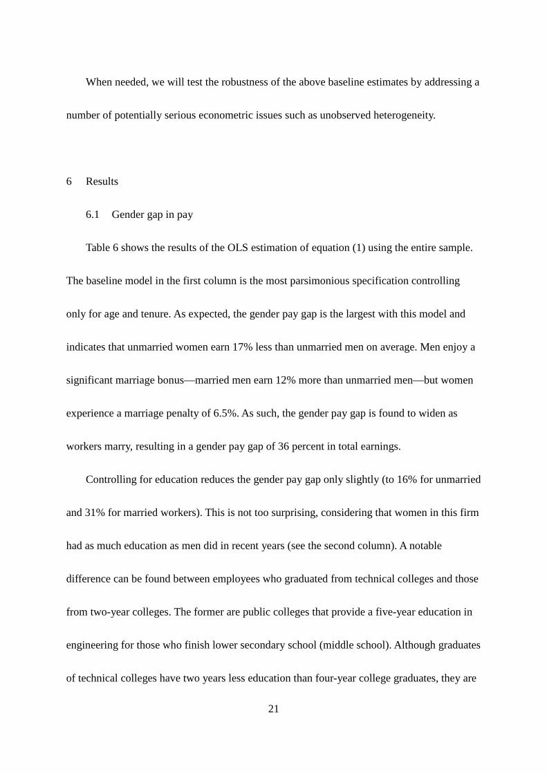
Table 6 shows the results of the OLS estimation of equation (1) using the entire sample.

The baseline model in the first column is the most parsimonious specification controlling

only for age and tenure. As expected, the gender pay gap is the largest with this model and

indicates that unmarried women earn 17% less than unmarried men on average. Men enjoy a

significant marriage bonus—married men earn 12% more than unmarried men—but women

experience a marriage penalty of 6.5%. As such, the gender pay gap is found to widen as

workers marry, resulting in a gender pay gap of 36 percent in total earnings.

Controlling for education reduces the gender pay gap only slightly (to 16% for unmarried

and 31% for married workers). This is not too surprising, considering that women in this firm

had as much education as men did in recent years (see the second column). A notable

difference can be found between employees who graduated from technical colleges and those

from two-year colleges. The former are public colleges that provide a five-year education in

engineering for those who finish lower secondary school (middle school). Although graduates

of technical colleges have two years less education than four-year college graduates, they are

22

treated almost equally as 4-year college graduates in terms of career path--most of them

advance to management trainee positions (i.e. SA and SB). In contrast, two-year colleges

provide liberal arts education to mostly women. Graduates of those junior colleges become

administrative support staff and typically follow the same career path as female high school

graduates, and rarely go beyond the J2 level. Only a few percent of them can switch to

management trainee positions (e.g. SA and SB job grades). Including a set of educational

level dummy variables allows us to account for the differing career implications of the above

two groups with seemingly similar lengths of education.

One important fact that we should keep in mind is that the company has changed job

design and pay systems a number of times since the Equal Employment Opportunity Act

(EEOA) became first effective in FY1987 with the last major reform implemented in FY2003.

The current job grade system was introduced the same year (FY2003). Assuming that the old

system was more discriminatory against women and the switch to the new job grade system

did not adjust the pay levels automatically for older employees who had entered the firm

many years before, the pay differences between male and females workers are expected to be

greater for older cohorts. In order to examine this prediction, we restrict our analysis to those

who graduated after FY1986in the third column. As expected, the estimated gender pay gap is

found to be 2-4 percentage points smaller for both the unmarried and the married after 1987.

23

In order to further investigate what factors are causing such a substantial gender pay gap,

we repeated the same regression analysis adding one additional control variable in each step.

Table 7 shows the results. Model 1 corresponds to column (1) in Table 7—accounting for

only age (fourth degree polynomial), tenure (quadratic), and fiscal year dummies. Model 2

includes additionally controls for education (column (2) in Table 7).

Model 3 further controls for the number of dependents (in the logarithm) to capture both

the direct effect on total earnings of dependent allowances as well as the indirect effect of

having dependents. This dependent allowances that favor workers with dependents is

reminiscent of the practices promoted by the government during wartime and is still prevalent

among large Japanese firms. As we discussed earlier, the existence of dependent allowances

directly increases both the marriage premium for men and the gender pay gap for the married

because in most married couple it is the husband who claims the dependent(s).7 Accounting

for the number of dependents reduces the marriage premium for men and the gender pay gap

for the married by 4-5%.

Model 4 additionally controls for job grade levels and job skill rank. Job grade levels are

determined based on the actual job assigned to the worker whereas job skill rank is

determined based on the supervisors’ evaluation of the worker’s skill level, which is part of

7 Generally speaking, it is more beneficial to claim a dependent for tax exemption for whoever earns more. We believe that husbands typically claim it in part due to the fact that they are more likely to earn more than their spouses. The payment of dependent allowance is based on the information on the tax documents.

24

the annual evaluation. Since job grades and job skill ranks are two of the most important

determinants of salary and bonus, adding the two has improved the R squared considerably

from 0.7766 to 0.9182, and reduced the gender pay gap substantially—by 8% and 9% for the

unmarried and the married, respectively. This means that a substantial part of the gender pay

gap is caused by slow promotion to higher job grade levels or differential job assignments for

female workers.8

In the next model, we additionally account for hours worked per year (hours), annual

reduced work hours (jitan meaning reduced hours in Japanese, arranged for employees with

needs to take care of their pre-elementary school age children), and annual late night hours

worked (yakan meaning night time in Japanese). The reason for including three variables is

that the implications for evaluation and promotion decisions may differ as well as different

rates that apply to ordinary overtime work, reduced work, and work during the night-time

shift. Note that the late night hours worked may also capture the different nature of job

contents. For example, both production workers and administrative support staff move up the

non-managerial track but the gender composition is strikingly different between production

workers and administrative support staff as the former is predominated by men and the latter

by women. Monthly salary could be significantly different between them due to differences

8 Skill rank is highly correlated with seniority and largely irrelevant to managerial track workers. Reassuringly it is found to be largely job grade not skill rank that matters for earnings and promotion for college graduates. These results as well as all other unreported results are available upon request from the corresponding author.

25

in benefits and premium pay for off-hour shifts for production workers. Surprisingly,

accounting for working hour variables almost eliminated the remaining unaccounted gender

pay gap. Now, the unaccounted pay gaps are only 0.3% (statistically insignificant) for the

unmarried and 3.5% for the married. Further controlling for evaluation (Model 6) does not

help to explain the gender pay gap.9

We also repeat the same exercise restricting our sample to only college graduates (we do

not include those with graduate degrees). Note that, in Model 2, we attempt to account for

some differences in worker human capital by including a university ranking category

variable.10 Similar to the result for the whole sample, the unaccounted gender pay gaps

shrink to 1.3% and 3.6% for the unmarried and the married, respectively, once job grade, job

skill ranks, and working hour variables are controlled for.

To sum up, most of the gender pay gap seems to be related directly or indirectly to

shorter hours worked and the slow promotion of female workers (job grade levels). Roughly

speaking, the twenty five to fifty percent of the gender pay gap that typical human capital

9 Our conclusion that evaluation does not account for the gender pay gap remain valid when we change the order of adding evaluation and hours variables--add evaluation before the hours variables. 10 Building on one of the most widely used university ranking in Japan--the Yoyogi-seminar’s university ranking (http://www.yozemi.ac.jp/rank/gakubu/index.html), we constructed a category variable where 1 indicates the 1st-tier national universities (Tokyo, Kyoto, Hitotsubashi, Osaka, Tokyo Institute of Technology, Tokyo University of Foreign Studies), 2 indicates the 2nd-tier national universities (Nagoya, Kobe, Tsukuba, Kyushu, Hokkaido, Tohoku, Ochanomizu, Yokohama National), 3 indicates the 1st-tier private universities (Keio, Waseda, Sophia, ICU), 4 indicates the 2nd-tier private universities (Gakushuin, Meiji, Aoyama Gakuin, Rikkyo, Chuo, Hosei, Tokyo University of Science, Doshisha, Ritsumeikan, Kansai Gakuin, Kansai, University of Occupational and Environmental Health), and 5 indicates all other universities.

26

variables (i.e. education, experience, tenure) cannot explain can be attributed to either factor.

For the remainder of the paper we will explore these two major culprits for the gender pay

gap and provide further insights on the gender gap in labor market outcomes.

6.2 How large is the maternity penalty?

Working hour variables account for thirteen percentage points of the gender pay gap for

the married. It is quite plausible that career interruptions or restrictions on work hours due to

childbirth and parenting are causing this link.

Table 8 summarizes the records of parental or family care leave taken between 1999 and

2009 by those in the sample. The company records do not distinguish between parental leave

and family care leave (mostly to care for the elderly). For women, however, mandatory

postnatal leave, which is differently coded due to the different funding source for the benefit,

always precedes parental leave. Therefore, we can surmise which leave is for parenting and

which is for other family members. There are two remarkable points to note about the

summary table. First, although we do not know the parental vs. family care leave composition

in the fourteen male cases, it is clear that few men take parental leave despite the fact that

men are equally eligible for parental leave.11 We suspect that social norms may be still

working against men who take parental leave in Japan (Fortin 2005). Second, the average

11 What is uniquely generous about the Japanese system is that both mother and father can take parental leave at the same time.

27

period of leave for women is fourteen months, although the actual leave varies widely from

two months to over two years. Third, a majority of women who have taken a leave don’t have

four-year college degrees, because the company did not hire female college graduates for

management trainee positions until the 2000s.

In order to evaluate the impact of career interruptions or restrictions on work hours due

to childbirth and parenting, we estimate OLS and fixed effect models similar to equation (1)

including variables summarizing parental leave history and hours worked. births is a category

variable indicating the number of prenatal/postnatal leave spells that each worker took in the

past and can be interpreted as the number of childbirths since 1999. Since there are only

seven cases of more than two childbirths, we combine cases of two or more spells as births =

2. The variable takes zero for all men. leave_pd is the accumulated length of leave (prenatal,

postnatal, parental and family care leave). We also add variables for the three types of hours

worked: hours worked per year (hours), reduced work hours (jitan) and night-time hours

worked (yakan) in the logarithm form.

Table 9 shows the results for all employees and a subsample of college graduates.

Compared with the second column of Table 7, the coefficients Marriage × Female are

substantially smaller in Column 1 and 2 of Table 9, indicating that some portion of the gender

pay gap estimated earlier in fact reflects the impact of career interruptions or restrictions on

work hours due to childbirth and parenting. More precisely, the gender pay gap for the

28

married was reduced from 31% to 26% after accounting for parental leave history and further

down to 18% after controlling for working hour variables. For the subsample of college

graduate workers, the role of childbirth and parenting may be much smaller because a

substantially smaller portion of this group have taken a parental leave. The gender pay gap

for the married in this subsample declined slightly from 21% (see Model 2 in the bottom of

Table 7) to 19% and 16% after accounting for leave history and hours worked, respectively.

The OLS estimates on the wage effects of the incidence of maternity leave and its lengths

do not appear to point to any clear conclusion. When the hours variables are not controlled

for, the estimated coefficients on leave_pd for both samples are negative and significant,

pointing to a wage penalty for those who do not return quickly to work from their maternity

leaves. However, once the hours worked are accounted for, the estimated coefficients on

leave_pd are no longer significant for either sample

However, leave_pd may be affected by unobserved worker characteristics, and if such

unobserved worker characteristics are correlated with wages, the estimated coefficients on

leave_pd will be biased. For instance, if the female employee with high innate ability is more

likely to have a husband with more demanding and high-paying jobs, she is more likely to

take a longer parental leave. If we fail to control for such innate ability of the female

employee, any negative wage effect of leave_pd will be offset by the positive wage effect of

her high innate ability. In other words, once we use individual fixed effects to control for such

29

time-invariant worker heterogeneity, we are likely to find the negative wage effect of

leave_pd.

Table 10 shows such fixed effect estimates (along with the OLS estimates). As expected,

the negative wage effect of leave_pd is underestimated in OLS (in fact, it is not significantly

different from zero). However, once unobserved worker heterogeneity is accounted for by

using individual fixed effects, the estimated coefficients on leave_pd are negative and

significantly different from zero. The fixed effect estimates provide several insights on the

role of maternity leave and working hours in the gender pay gap. First, we find a non-linear

maternity penalty. Namely, the decline in wage income is not proportional to the length of the

time out. The coefficient of the indicator of births=1 is significantly positive in the fixed

effect models for women (Column 2 and 3). According to the estimation result in Column 3, a

female worker who gives birth will not experience any decline in income as long as she

comes back from leave within seven months and works for the same hours as before.

However, as she delays her return from her maternity beyond seven months, there will be a

maternity penalty (wage decline) and the size of the maternity penalty will continue to

increase as she keeps delaying her return.

Second, the estimated coefficients on leave_pd are much smaller once hours worked is

accounted for. This indicates that a much larger portion of the maternity penalty can be

attributed to the restrictions on work hours after returning from leave rather than the leave

30

itself. You can see this picture in the top portion of Table 12 where we calculated the impact

of time out on total pay for the average female worker. If a female worker takes twelve

months of leave at her first childbirth, she is likely to lose 17% of income after coming back

to work but most of the income drop will be due to shorter hours worked and the use of the

reduced work hour benefit for working mothers.

Third, by comparing the impacts of time out between women and men, we see that time

out is more detrimental for men than for women. Men typically lose 7-11% of their income

after taking only a three month leave depending on whether their hours worked afterwards are

affected or not. This finding is consistent with Albrecht et al. (1998) who found a similar

result using Swedish data. The plausible explanation is that since taking leave is so unusual

for men in Japanese firms, doing so has a very negative signaling effect—superiors interpret

the action as signaling the person’s low commitment to work.

Table 11 presents the results of the same analyses for a subsample of college graduates.

The coefficients clearly indicate that the maternity penalty is much greater for college

graduate women. For this group, even those who return right after the minimum two months

of mandatory postnatal leave suffer income loss on average (Column 2) although this effect is

somewhat muted when hours worked are controlled for. Since there are only a few female

college graduates who have taken maternity leave twice in the dataset, the dummy variable

for births=2 was dropped in some specifications.

31

We find two sharp contrasts between our whole sample analysis and the college graduate

sample analysis: (1) the maternity penalty does not decline even after accounting for hours

worked; and (2) the maternity penalty is not greater for men any more. The bottom rows of

Table 12 clearly show that those educated women suffer 20% of loss in income per year of

parental leave and shorter hours worked do not seem to be associated with the maternity

penalty. We speculate that jobs for college graduates are most affected by technological

development and relation-specific knowledge, and thus that the depreciation of their human

capital is faster. Therefore, their positions may be more likely to be assumed by somebody

else when they return from parental leave, and they might lose substantial task-specific

human capital.

A substantial maternity penalty for female college graduates is also explained by their

career track change before and after their maternity leave. Our interviews with HR managers

indicated that jobs or career tracks are heterogeneous, and not all female college graduates

are in management trainee positions. Suppose there are high wage growth jobs and low wage

growth jobs. The former requires a high commitment and includes a possibility of relocation.

Thus, many pregnant women or those with small children in the former group may change

their jobs from a high commitment/wage growth job to a low commitment/wage growth job.

Since this kind of job change is also associated with longer parental leave, the estimated

maternity penalty increases.

32

Whatever the explanation, our result is consistent with Bertrand, Goldin and Katz (2010)

who found that the gender pay gap is associated with career interruptions due to parenting.

Since their dataset consists of highly educated women (MBAs from a top school), career

interruptions may be especially costly.

In sum, the incidence of childbirth and the choice of parental leave periods could affect

the observed wage levels through multiple channels. First, having a small child will lead to

fewer hours worked due to the competing demand of childcare. Second, the expectation of

fewer work hours and a weaker commitment, or a demonstration of a high commitment

through the choice of a shorter leave period may result in a change in job assignment to one

with less or more responsibility. Such a job change would not only be preferred by the firm

but also may be favored by the worker herself, who needs to balance dual responsibilities.

The provision of training may also change accordingly. Third, the different costs of

childbearing and career interruption by career tracks will affect the initial choice of job and

the timing of childbearing, which in turn affects our estimation of the impact of childbirth on

wage income.

The purpose of including hours worked as a control is to distinguish the effect of reduced

hours on wage from the effects through career track selection. The substantial difference

between the entire sample and the subsample of college graduate women seems to suggest

that the above impact of time away is predominantly caused by the first channel for less

33

educated women while the career track selection is much more important for highly educated

women.

6.3 The Gender Gap in Promotion

Table 13 shows the results from our initial analysis of the gender gap in promotion using

an ordered logit model estimation of job grade levels. Consistent with our results of the OLS

estimation of wage function, job grade levels are consistently found to be negatively

correlated with femaleness after accounting for education and experience, and the gender gap

is greater for the married. The results are robust to the inclusion of leave history variables and

evaluation grades and the restriction to college graduates. For our analysis using the

subsample of college graduates, we account for school quality by including the university

ranking category variable as a control.

One important finding in this table is that women who receive the highest evaluation are

no significantly more likely to get promoted than those who receive an average evaluation.

Thus, while the estimated coefficient on A1 or better is positive and significant, the estimated

coefficient on the interaction term involving female and A1 or better is negative and

significant, almost completely offsetting the positive coefficient on A1 or better. It follows

that getting better evaluation will help male employees get promoted whereas getting better

34

evaluation has no beneficial effect for promotion of female employees. It other words,

women face a glass ceiling or are in jobs with no prospects for promotion.

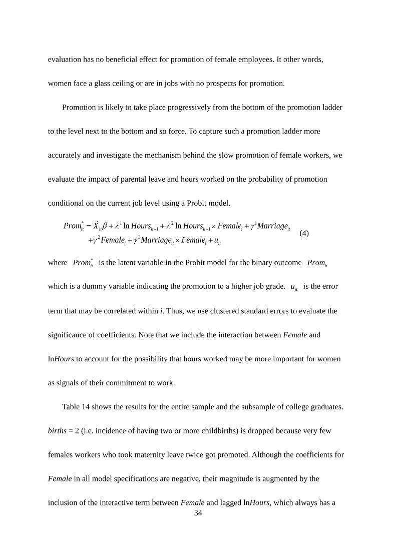
Promotion is likely to take place progressively from the bottom of the promotion ladder

to the level next to the bottom and so force. To capture such a promotion ladder more

accurately and investigate the mechanism behind the slow promotion of female workers, we

evaluate the impact of parental leave and hours worked on the probability of promotion

conditional on the current job level using a Probit model.

* 1 2 11 1

2 3

ln lnit it it it i it

i it i it

Prom X Hours Hours Female MarriageFemale Marriage Female uβ l l g

g g− −= + + × +

+ + × +

(4)

where *itProm is the latent variable in the Probit model for the binary outcome itProm

which is a dummy variable indicating the promotion to a higher job grade. itu is the error

term that may be correlated within i. Thus, we use clustered standard errors to evaluate the

significance of coefficients. Note that we include the interaction between Female and

lnHours to account for the possibility that hours worked may be more important for women

as signals of their commitment to work.

Table 14 shows the results for the entire sample and the subsample of college graduates.

births = 2 (i.e. incidence of having two or more childbirths) is dropped because very few

females workers who took maternity leave twice got promoted. Although the coefficients for

Female in all model specifications are negative, their magnitude is augmented by the

inclusion of the interactive term between Female and lagged lnHours, which always has a

35

positive coefficient. Note that the coefficients on one maternity leave spell (birth=1) and

accumulated length of leave (leave_pd) are negative as expected although neither is

significant (Column 1). The coefficient of leave_pd is reduced substantially but becomes

significant after working hour variables are controlled for (Column 2). This implies that

childbirth delays the promotion of female workers through two channels—career interruption

itself and a reduction in work hours after returning from the leave. Adding evaluation grades

as a control does not change the overall picture (Column 3). We also see a similar pattern for

college graduates (Column 4-6)

The positive and significant coefficient of Female × lagged lnHours in all specifications

clearly indicates that hours worked plays a more important role in the promotion decisions for

women than for men. The relationship between hours worked and the odds of promotion may

not be linear. Using the U.S. National Longitudinal Survey of Youth, Gicheva (2010) finds

that the relationship between hours worked and wage growth is non-linear—only workers

who put forth more hours than a certain threshold see the positive impact of working

additional hours. To investigate such possible non-linearity, we re-estimate the model in

equation (4) replacing 1ln −itHours with a categorical variable 1_ −itcatHours which takes 1

if hours worked is less than 1800 hours per year; 2 if it is 1800 or more but less than 1900, 3

if it is 1900 or more but less than 2000, 4 if it is 2000 or more but less than 2100, 5 if it is

36

2100 or more but less than 2200, 6 if it is 2200 or more but less than 2400, and 7 if it is 2400

hours or more.

Figure 4 illustrates the predicted odds of promotion for each categorical value of

1_ −itcatHours averaged over subsamples of men and women (4-1) and averaged over the

subsamples of college graduate men and women (4-2). They imply that, for men, working

extra hours affect the odds of promotion only when hours worked exceed 2200 hours per year

but, for college graduate men, hours worked do not seem to affect the odds of promotion. For

women, there is much stronger relationship between the two in every level of hours worked

but the impact of working extra hours is especially strong when hours worked exceed 2200

hours per year. What is interesting is that, except for the group of employees who work less

than 1800 hours, women who work the same hours as men have higher odds of promotion

than men. Although we are not comparing men and women with the same characteristics in

Figure 4 (i.e. averaged separately over subsamples), comparing men and women with the

same characteristics (i.e. averaged over the entire sample at female=[0,1]) does produce the

same pattern.

This contrast between men and women may imply that the revealed preference for long

work hours does not affect the perceived competence of male college graduates but does so

for female college graduates. Note that working long hours could be associated with a

worker’s commitment to work, the assignment of challenging tasks, or low productivity.

37

Therefore, we do not have an a priori expectation about how hours worked should be

associated with promotion probability. It is plausible however, that by working longer, a

female worker can credibly signal her commitment to work and demonstrate that her

competing demands of housework and childcare do not affect her performance.

Another possibility is that the stark difference between men and women in the

association of longer hours with promotion the following year may be simply reflecting job

segregation. Many authors, including Blau and Kahn (2000) have reported that women were

concentrated in administrative support and service occupations.12 Some college-educated

women may be assigned to jobs with little training and promotion prospects while others join

college-educated men in management trainee jobs. If women in the former group have no

reasonable promotion prospects, they will not work long hours. Combining members from

the two groups may result in a high correlation between the odds of promotion and hours

worked.

We can eliminate the bias caused by job segregation to the extent to which good jobs and

bad jobs are separated into different organizational units by estimating the model with

organizational unit fixed effects. A typical organization unit is a section of 3-9 people for

white-collar workers and a group of people working on the same production line or support

12 Historically in Japan, women were typically assigned to administrative support and clerical jobs called ippan-shoku (general job), while college educated men were assigned to management trainee positions called sogo-shoku (composite job). Although such differentiation was prohibited by the EEOA, a similar pattern of task assignment may still remain.

38

function (up to 90) for blue-collar workers. We employ a conditional (fixed effects) logit

model. Note that we have a set of workers (i = 1,2,…,n) who are grouped into organizational

units (j = 1,2,…,J). Consider the following logistic regression model:

log( )1

ijti ijt i

ijt

pX

pµ β α= + +

−

where ijtp is the probability that worker i in group j gets promoted in period t, tµ is

the intercept that may be different for each period t, ijtX is a vector of predictors that may

vary across workers or across time, and iα represents the combined effects of all

unobserved characteristics of each organizational unit. It is well-known that the log

likelihood function for this logistic regression model, conditional on the number of

promotions within the same organizational unit being the actual number observed, does not

contain iα and the coefficients of Maximum Likelihood Estimation is consistent.

The results of this conditional (fixed effects) logit model presented in Table 15 are

qualitatively almost identical with the probit model estimation results in Table 14 except that

for college educated women the maternity penalty is significant and much more distinct but

taking long parental leave is not necessarily detrimental. A comparison between the probit

estimation and fixed effects logit estimation presents several implications. First, the high

correlation between the odds of promotion and hours worked among women is not driven by

the fact that women who are assigned to workplaces with good promotion prospects work

longer hours. The same result is obtained even when we focus on the variation within

39

organizational units. Second, longer hours worked are now negatively correlated with odds of

promotion for men, although this result does not hold when the sample is restricted to college

graduates. This result suggests that, at least for lower skilled workers, longer hours signal low

productivity when two employees working side by side are compared. Third, the earlier

finding that women who take longer parental leaves receive lower earnings in the future

primarily comes from the variation across organizational units. Hence, it may be the case that

women who are in jobs with less training and less promotion prospects are more likely to take

longer parental leaves. This result must be interpreted with caution, however, because it is

quite possible that those who take longer parental leaves may be transferred to jobs with little

promotion prospects after returning to work (thus within organizational unit variation does

not affect the odds of promotion).

6.4 Gender Gap in Evaluation

Finally, we estimate the ordered logit model using the employee’s evaluation as the

dependent variable to see if there are any gender differences in evaluation that cannot be

accounted for by other variables. Table 16 presents the results. Job grades are controlled for

because the company’s “management by objectives” policy requires the evaluator and the

40

evaluated to set objectives in accordance with performance standards and level of

responsibilities expected for the job grade level.

Although evaluation grades are positively associated with education, they are negatively

associated with many variables that are known to be positively correlated with wage and

promotion, such as marriage and hours worked. Although unmarried women tend to receive

lower evaluations than unmarried men, married women tend to obtain no worse evaluations

than married men. These results may be consistent with the statistical discrimination

explanation. Unmarried women receive less training because there is a greater uncertainty

about their commitment, but such discrimination disappears after they stay at their jobs after

marriage and show commitment over time. But this explanation does not explain why

married men receive lower grades. One plausible explanation is that the company’s

evaluation mainly measures job-specific or task-specific human capital. Workers who are

more likely to get promoted (e.g. married men, those who work long hours, etc.) have been

on a specific job for a shorter amount of time and have accumulated less task-specific human

capital and thus receive lower evaluation grades. On the other hand, workers who have been

on the same job for a long time (e.g. married women with small children choosing reduced

work hours) have accumulated a lot of task-specific human capital, and thus receive relatively

higher grades.

41

This interpretation is consistent with institutional details on how the evaluation system is

designed. The company employs “management by objectives” and therefore, good

evaluations indicate that the employee achieved many of his/her objectives for the year. The

evaluator does not evaluate the worker’s competency as a manager nor are the evaluation

results used directly for promotion. Therefore, the variable purely measures the job-specific

and task-specific performance and mainly affects the bonus amount in the following year.

Overall, we find little evidence that evaluation is a main driver of the gender gap in pay and

promotion (this is particularly true for college graduates).

7 Conclusion

The gender pay gap is a persistent nature of every country’s labor market (Blau 2003)

and it is especially large and tenacious in the Japanese labor market. This gender gap may be

caused by the actual and expected human capital loss due to career interruptions, as well as

different jobs and skills men and women choose to acquire. Using detailed personnel records

from a large Japanese manufacturing firm, we have attempted to identify the sources of the

large intra-firm gender gap observed in the firm. We find 19% and 28% gender pay

differences among unmarried employees and married ones, respectively, after controlling for

basic human capital variables. The gender gap declines substantially when accounting for job

levels and hours worked. The unaccounted portion of the gender pay gap is likely to be

42

mostly caused by differences in unobserved job contents. When we restrict our analysis to

college graduate employees, the gender pay gap is only a few percentage points once job

levels and hours worked are controlled for. As such, most of the gender pay gap among

employees on the management track is caused by fewer hours worked and slower promotion

among women.

As primary mechanisms behind the slow promotion of women, we have sought evidence

on two theories explained by the competing demands of housework/childcare, and statistical

discrimination. The data generally have supported the competing demands explanation. A

substantial component of the gender gap in pay and promotion for married workers is

explained by shorter hours worked and parental leave history. Furthermore, our probit

analysis of promotion has revealed that lagged hours worked is the most important predictor

of the gap, together with evaluation grades.

We have also found some evidence for statistical discrimination. First, the maternity

penalty is non-linear. Female workers who return to work after a short parental leave is

subject to no maternity penalty, but taking a long parental leave or having two childbirths

results in a significant loss in income and a much lower chance of promotion thereafter.

Women may effectively signal their commitment to work by returning from parental leave

within six months. Second, the promotion of female workers is much more strongly

correlated with hours worked in the previous year. This finding may indicate that women can

43

ease the concerns of their superiors about their commitment to work by working longer hours,

but such signaling is not necessary for men. Furthermore, such correlation between

promotion and lagged hours worked is lower and insignificant for male college graduates

whereas it is even higher in the case of women. It may be the case that the required human

capital investment is higher for management trainees, and thus signaling private information

regarding commitment and the competing demands of housework is more important for

college educated women.

Our findings are different from Gicheva (2010) who reports that the slope of the

relationship between hours worked and wage growth differs little between men and women,

whereas they are quite different in our study. What is striking in our findings is that the slope

is very flat for men but it is significantly steep for women. The learning-by-doing model used

in Gicheva (2010) cannot explain our results.

Although we interpret the high correlation between long hours worked and odds of

promotion as indicating evidence of signaling, we actually do not know whether the long

hours worked are due to the employee’s choice or to the employer’s job assignment decision.

For example, there are at least two more possible interpretations, both of which depict the

situation caused by asymmetric information.

First, as discussed in Landers, Rebitzer, and Taylor (1996), the firm may impose the

“overwork” norm and use the information of each worker’s hours to sort out workers with a

44

high propensity to work hard when making decisions on promotion. This interpretation is

close to the idea of rat-race equilibrium first proposed by Akerlof (1976).

The second interpretation is in line with Prendergast (1992) who studied situations where

the employer has private information about worker ability. Namely, a manager who identifies

a capable woman would assign her a challenging task to credibly signal her positive prospect.

Such signaling may be desirable if most women are discouraged and are not willing to work

long hours due to their perception that women are discriminated against. On the other hand, if

men are generally committed to work, equal treatment may be desirable because providing

more training (i.e. by assignment a challenging task) to a small number of selected men may

discourage other male workers. In other words, both separation and pooling may arise as

equilibria for women and men, respectively. In this interpretation, the causality is in the

opposite direction—a female worker who has better promotion prospects works long hours.

In future work, we plan to examine which of these three theories best fits our data.

45

References Abe, Yukiko. 2010 “Equal Employment Opportunity Law and the Gender Wage Gap in Japan: A Cohort Analysis,” Journal of Asian Economics 21: 142-155. Akerlof, George. 1976 “The Economics of Caste and of the Rat Race and Other Woeful Tales,” Quarterly Journal of Economics 90(4): 599-617. Albrecht, James W.; Edin, Per-Anders; Sundstrom, Marianne; and Vroman, Susan B. 1998 “Career Interruptions and Subsequent Earnings: A Reexamination Using Swedish Data,” The Journal of Human Resources 34(2): 294-311. Arrow, Kenneth. 1973. “The Theory of Discrimination.” In: Discrimination in Labor Markets, edited by O.A. Ashenfelter and A. Rees, pp. 3-33. Princeton, NJ: Princeton University Press. Barnett, William P.; Baron, James N., and Stuart, Toby E. 2000. “Avenues of Attainment: Occupational Demography and Organizational Careers in the California Civil Service.” American Journal of Sociology 106(1): 88-144. Becker, Gary S. 1957. The Economics of Discrimination. Chicago, IL: University of Chicago Press. Becker, Gary S. 1985. “Human Capital, Effort, and the Sexual Division of Labor,” Journal of Labor Economics 3 (January, suppl.): 33-58. Bertrand, Marianne; Goldin, Claudia, and Katz, Lawrence. 2010 “Dynamics of the Gender Gap for Young Professionals in the Financial and Corporate Sectors,” American Economic Journal: Applied Economics 2 (July): 228-255. Blau, Francine D., and DeVaro, Jed. 2006 “New Evidence on Gender Differences in Odds of promotion: An Empirical Analysis of a Sample of New Hires” NBER Working Paper 12321. Blau, Francine D. and Kahn, Lawrence M. 2000. "Gender Differences in Pay." Journal of Economic Perspectives. 14(4): 75-99. Blau, Francine D. and Kahn, Lawrence M. 2003 “Understanding International Differences in the Gender Pay Gap,” Journal of Labor Economics 21(1): 106-144.

46

Budig, Michelle, and England, Paula. 2001 “The Wage Penalty for Motherhood,” American Sociological Review 66 (April): 204-225. Cabral, Robert, Marianne A. Ferber, and Carole Green. 1981. “Men and Women in Fiduciary Institutions: A Study of Sex Differences in Career Development,” Review of Economics and Statistics 63 (November): 573-580. Cannings, Kathy. 1988. “Managerial Promotion: The Effects of Socialization, Specialization, and Gender.” Industrial and Labor Relations Review 42 (October): 77-88. Corcoran, Mary and Greg J. Duncan. 1979 “Work History, Labor Force Attachment, and Earnings Differences Between the Races and Sexes,” Journal of Human Resources 14(1): 3-20. Cobb-Clark, Deborah A. 2001. “Getting Ahead: The Determinants of and Payoffs to Internal Promotion for Young U.S. Men and Women.” In Solomon W. Polachek, ed., Worker Wellbeing in a Changing Labor Market (Research in Labor Economics 20):339-372. Edward, Linda N. 1988. “Equal Employment Opportunity in Japan: A View from the West.” Industrial and Labor Relations Review, 41(2): 240-249. Fortin, Nicole M. 2005. "Gender Role Attitudes and the Labour-market Outcomes of Women across OECD Countries," Oxford Review of Economic Policy, 21(3): 416-438. Gicheva, Dora. 2010 “Working Long Hours and Early Career Outcomes in the High-End Labor Market,” working paper, University of North Carolina at Greensboro. Gronau, Reuben. 1988 “Sex-related Wage Differentials and Women’s Interrupted Labor Careers—the Chicken or the Egg.” Journal of Labor Economics 6(3): 277-300. Landers, Renee M., James B. Rebitzer, and Lowell J. Taylor. 1996 “Rat Race Redux: Adverse Selection in the Determination of Work Hours in Law Firms.” American Economic Review, 86(3): 329-348. Lazear, Edward P., and Sherwin Rosen. 1990. “Male-Female Wage Differentials in Job Ladders,” Journal of Labor Economics 8(1): 106-123.

47

Light, Audrey, and Ureta, Manuelita. 1995. “Early-Career Work Experience and Gender Wage Differentials.” Journal of Labor Economics 13(1): 121-154. Manchester, Colleen F., Lisa M. Leslie, and Tae-Youn Park. 2008 “Screening for Commitment: the Effect of Maternity Leave Usage on Wages,” working paper, University of Minnesota. Mincer, Jacob, and Solomon Polachek. 1974. “Family Investments in Human Capital: Earnings of Women.” Journal of Political Economy 82(2) Part II: S76-S108. Paulin, Elizabeth A., and Jennifer M. Mellor. 1996. “Gender, Race, and Promotions within a Private-Sector Firm.” Industrial Relations 35(2): 276-295. Pekkarinen, Tuomas, and Juhana Vartiainen. 2004. “Gender Differences in Job Assignment and Promotion on a Complexity Ladder of Jobs.” IZA Discussion paper, no. 1184 (June). Phelps, Edmund S. 1972. “The Statistical Theory of Racism and Sexism,” American Economic Review 62, no.4: 659-661. Prendergast, Candice J. 1992. “Career Development and Specific Human Capital Collection.” Journal of the Japanese and International Economies 6: 207-227. Ransom, Michael, and Ronald L. Oaxaca. 2005. “Intrafirm Mobility and Sex Differences in Pay,” Industrial and Labor Relations Review 58(2) (January): 219-37. Waldfogel, Jane. 1997. “Working Mothers Then and Now: A Cross-Cohort Analysis of the Effects of Maternity Leave on Women’s Pay.” in Gender & Family Issues in the Workplace, edited by Francine D. Blau and Ronald G. Ehrenberg, pp 92-126. New York: Russell Sage Foundation.

48

Figure 1 Gender Pay Gap Measured by Hourly Wage in Japan.

Note: Based on the Basic Survey of Wage Structure by MHLW.

Table 1 Employee Composition by Gender and Marital Status

Fiscal Year Single Men Married Men Single Women Married Women without Small

Children

Married Women with Small Children*

Total

2004 18.6% 70.6% 5.9% 4.4% 0.6% 100% 2005 19.3% 69.8% 5.5% 4.2% 1.2% 100% 2006 21.6% 67.5% 5.5% 3.8% 1.6% 100% 2007 23.2% 65.6% 5.8% 3.6% 1.8% 100% 2008 25.5% 63.4% 5.5% 3.5% 2.0% 100% 2009 25.8% 63.0% 5.5% 3.5% 2.2% 100%

Note: Includes only regular workers. * shows the number of female workers who have taken parental leave after FY1998. This group also includes those who got divorced after having children.

0.55

0.57

0.59

0.61

0.63

0.65

0.67

0.69

0.7119

8119

8319

8519

8719

8919

9119

9319

9519

9719

9920

0120

0320

0520

0720

09

49

Table 2 Annual Wage, Average Age, Hours Worked by Gender and Marital Status Average Annual Wage

Fiscal Year Single Men Married Men Single Women Married Women without Small

Children

Married Women with Small Children*

2005 5,900,233 8,087,088 5,222,444 5,157,902 4,403,632 2006 5,961,231 8,198,714 5,402,587 5,405,735 4,471,967 2007 5,922,937 8,265,332 5,582,436 5,763,785 4,839,741 2008 5,803,538 8,186,499 5,469,831 5,811,252 4,825,612 2009 5,275,211 7,570,200 5,057,443 5,437,273 4,560,014

Average 5,772,630 8,061,567 5,346,948 5,515,189 4,620,193

Average Age

Fiscal Year Single Men Married Men Single Women Married Women without Small

Children

Married Women with Small Children*

2005 34.9 44.4 37.3 36.7 34.8 2006 34.7 44.3 37.9 37.6 35.0 2007 34.0 43.9 38.0 38.9 36.2 2008 33.3 43.4 37.7 39.9 36.5 2009 32.9 43.1 38.2 40.4 37.4

Average 33.9 43.8 37.8 38.7 36.0

Average Hours Worked per Year

Fiscal Year Single Men Married Men Single Women Married Women without Small

Children

Married Women with Small Children*

2005 2,072 2,060 1,922 1,794 1,667 2006 2,090 2,073 1,945 1,821 1,640 2007 2,095 2,091 1,950 1,838 1,588 2008 2,112 2,089 1,919 1,821 1,613 2009 2,059 2,034 1,854 1,782 1,588

Average 2,086 2,069 1,918 1,811 1,619 Note: The figures in the table only include those who work for twelve months in each fiscal year. Hence, women who took a parental leave in the fiscal year are not included.

Table 3 Distribution of Men and Women by Education levels Men

Year of Hiring

Ph.D. Master BS/BA Tech.

College 2-yr.

college Vocatio-nal Sch.

High School

Middle School

UNK Total

1990-99 1.8% 18.5% 23.0% 7.2% 0.7% 3.7% 44.2% 0.8% 0.1% 100.0% 2000-09 3.8% 19.7% 28.5% 3.2% 0.9% 5.0% 30.6% 0.2% 8.0% 100.0%

Women

Year of Hiring

Ph.D. Master College College of Tech.

2-y college

Vocational Sch.

High School

Middle School

UNK Total

1990-99 0.3% 3.3% 14.8% 1.3% 37.2% 9.5% 33.4% 0.0% 0.3% 100.0% 2000-09 4.2% 26.7% 28.3% 3.3% 3.6% 20.2% 5.5% 0.0% 8.1% 100.0%

Note: Employees hired before 2004 include only those who were still employed in 2004. UNK stands for unknown.

50

Figure 2 Promotion Path Chart

J1

J2

J3

J4

JH SA

SB

G6

G5

G4

G3

G2

G1

Blue-Collar Track (High School Graduates)

White-Collar Track (College Graduates)

51

Table 4 Distribution of Men and Women in Hierarchy As of 2004

Job Grades Single Men Married Men Single

Women

Married Women without Small

Children

Married Women with Small Children*

Total

J1 3.09% 1.77% 0.30% 0.08% 0.00% 5.24% J2, J3 8.88% 27.73% 4.89% 3.63% 0.57% 45.68% SA, J4 2.29% 8.64% 0.31% 0.11% 0.01% 11.37% SB, JH 1.54% 4.56% 0.11% 0.11% 0.00% 6.33%

G6 1.10% 4.04% 0.13% 0.25% 0.03% 5.55% G5 1.22% 10.61% 0.14% 0.17% 0.00% 12.14% G4 0.44% 8.71% 0.03% 0.08% 0.00% 9.26% G3 0.08% 3.53% 0.01% 0.00% 0.00% 3.63%

G1,G2 0.01% 0.79% 0.00% 0.00% 0.00% 0.81% Total 18.66% 70.36% 5.92% 4.45% 0.61% 100.00%

Managers 202 1,954 22 36 2 2,216 (G6 or higher) 9.1% 88.2% 1.0% 1.6% 0.1% 100.0%

Senior Managers 38 920 3 6 0 967 (G4 or higher) 3.9% 95.1% 0.3% 0.6% 0.0% 100.0%

As of 2009

Job Level Single Men Married Men Single

Women

Married Women without Small

Children

Married Women with Small Children*

Total

J1 6.91% 3.04% 0.59% 0.11% 0.01% 10.63% J2, J3 8.77% 20.65% 3.36% 2.32% 1.78% 36.85% SA, J4 4.94% 8.17% 0.93% 0.37% 0.10% 14.52% SB, JH 2.45% 4.84% 0.32% 0.17% 0.15% 7.93%

G6 0.92% 4.06% 0.13% 0.15% 0.15% 5.42% G5 1.15% 8.07% 0.14% 0.18% 0.04% 9.58% G4 0.64% 9.51% 0.08% 0.13% 0.00% 10.34% G3 0.11% 3.81% 0.00% 0.04% 0.00% 3.96%

G1,G2 0.01% 0.77% 0.00% 0.00% 0.00% 0.78% Total 25.91% 62.92% 5.54% 3.47% 2.23% 100.00%

Managers 222 2,053 27 39 15 2,355 (G6 or higher) 9.4% 87.2% 1.1% 1.7% 0.6% 100.0%

Senior Managers 60 1,103 6 13 0 1,181 (G4 or higher) 5.1% 93.4% 0.5% 1.1% 0.0% 100.0%

52

Table 5 Frequency of Promotion by job level, gender, and marital status (2004-2009)

Single Men Married Men Men Total

Job Grades

# of employees

Freq. of promotions

Promotion rate

# of employees

Freq. of promotions

Promotion rate

# of employees

Freq. of promotions

Promotion rate

J1 2646 696 26.3% 1241 277 22.3% 3887 973 25.0%

J2, J3 3746 136 3.6% 10495 515 4.9% 14241 651 4.6%

SA, J4 1483 227 15.3% 3721 242 6.5% 5204 469 9.0%

SB, JH 830 103 12.4% 2024 265 13.1% 2854 368 12.9%

G6 436 65 14.9% 1669 298 17.9% 2105 363 17.2%

G5 559 41 7.3% 4146 485 11.7% 4705 526 11.2%

G4 238 12 5.0% 4069 280 6.9% 4307 292 6.8%

G3 51 2 3.9% 1659 106 6.4% 1710 108 6.3%

Single Women

Married Women without Small Children

Married Women with Small Children* Women Total

Job Grades

# of employees

Freq. of promotions

Promotion rate

# of employees

Freq. of promotions

Promotion rate

# of employees

Freq. of promotions

Promotion rate

# of employees

Freq. of promotions

Promotion rate

J1 215 130 60.5% 40 18 45.0% 6 2 33.3% 261 150 57.5% J2, J3 1782 38 2.1% 1281 15 1.2% 606 2 0.3% 3669 55 1.5% SA, J4 280 35 12.5% 96 14 14.6% 24 0 0.0% 400 49 12.3% SB, JH 83 7 8.4% 57 10 17.5% 31 1 3.2% 171 18 10.5%

G6 54 6 11.1% 93 9 9.7% 43 1 2.3% 190 16 8.4% G5 69 4 5.8% 80 4 5.0% 11 0 0.0% 160 8 5.0% G4 18 0 0.0% 37 2 5.4% 0 0 0.0% 55 2 3.6% G3 5 0 0.0% 15 0 0.0% 0 0 0.0% 20 0 0.0%

53

Figure 3 Separation rate by age, gender, and marital status

0.0%

2.0%

4.0%

6.0%

8.0%

10.0%

12.0%

14.0%

192123252729313335373941434547495153555759

Single MenMarried MenSingle WomenMarried WomenTotal

54

Table 6 OLS Estimation of Gender Pay Gap Dependent variable ln(total pay)

Base w. education Graduated in

FY1987 and after Marriage 0.1214 *** 0.1078 *** 0.0991 *** -0.0054

-0.0043

(0.0044)

Female -0.1708 *** -0.1602 *** -0.1240 *** -0.0091

-0.0084

(0.0091)

Marriage × Female -0.1858 *** -0.1504 *** -0.1687 *** -0.014

-0.0114

(0.0118)

Education (base: high school)

Ph.D.

0.3955 *** 0.3099 ***

-0.0108

(0.0110) Master’s degree

0.3324 *** 0.2435 ***

-0.0047

(0.0056) BS/BA

0.2127 *** 0.1338 ***

-0.0058

(0.0057) Technical College

0.1566 *** 0.1020 ***

-0.0058

(0.0061) 2-year college

-0.0252 *** -0.0708 ***

-0.0086

(0.0092) Middle school

-0.1213 *** 0.0188

(0.0083)

(0.0826) Vocational school

0.0202 ** -0.0227 **

(0.0089)

(0.0097) Vocational school (medical)

0.1490 *** 0.0879 ***

(0.0136)

(0.0136) Control for age and tenure Yes Yes Yes Control for fiscal year Yes Yes Yes R2 overall 0.6546 0.7743 0.8024 Number of observations 42073 42071 23728

55

Table 7 Explaining the Gender Pay Gap Dependent Variable: ln(total earnings) All Employees Independent variables R2 Gender Pay Gap/Marriage Premium

Single Married Marriage P. for Men

Model 1 Age, tenure, and f. year dummies

0.6546 -0.1708 -0.3566 0.1214

Model 2 ＋education 0.7743 -0.1602 -0.3107 0.1078

Model 3 ＋# of dependents 0.7766 -0.1656 -0.2568 0.0637

Model 4 ＋job grade, job skill rank 0.9182 -0.0886 -0.1668 0.0381

Model 5 ＋hours worked 0.9593 -0.0028 -0.0349 0.0393

Model 6 + evaluation 0.9596 -0.0052 -0.0356 0.0382

College Graduates only Independent variables R2 Gender Pay Gap/Marriage Premium

Single Married Marriage P. for Men

Model 1 Age, tenure, and f. year dummies

0.7297 -0.1708 -0.2276 0.1123

Model 2 ＋university ranking 0.7936 -0.1496 -0.2135 0.1000

Model 3 ＋# of dependents 0.7962 -0.1445 -0.1643 0.0575

Model 4 ＋job grade, job skill rank 0.9341 -0.0516 -0.0764 0.0453

Model 5 ＋hours worked 0.9571 -0.0128 -0.0363 0.0504 Model 6 ＋evaluation 0.9571 -0.0104 -0.0322 0.0491

Note：The figures are the coefficients in the estimated Mincerian wage function using the total compensation (monthly salary and bonus). Includes only regular employees who were in the payroll for twelve months.

56

Table 8 Use of Parenting/Family Care Leave by Type and Employee Characteristics Women Men # of employees in the sample 1022 8602 Those who have taken a leave 271 14 Average period 13.80 3.07 Type of leave Prenatal/postnatal/parental 187

N.A.

# of times leave was taken 1 142 2 38 3 6 4 1

Family care 84 By education level PhD 4 1 MS/MA 16 1 BS/BA 35 5 2-y college 78 0 High School 106 5 Others 32 2 Ave. Age in 2009 or at the exit 37.3 42.9

57

Table 9 Estimation of the Impact of Time Out on Wage Income Dependent Variable: All Employees College Graduates

ln(total wage) OLS OLS

Marriage 0.0797 *** 0.0584 *** 0.0852 *** 0.0621 ***

(0.0048)

(0.0050) (0.0126)

-0.0128

Female -0.1772 *** -0.1536 *** -0.1331 *** -0.157 ***

(0.0088)

(0.0097) (0.0211)

-0.0237

Marriage × Female -0.0802 *** -0.0291 ** -0.0534

-0.0063

(0.0138)

(0.0149) (0.0484)

-0.053

One maternity leave spell

(births=1)

0.0106

0.0572 *** 0.0963

0.116

(0.0216)

(0.0176) (0.0734)

-0.0942

Two or more maternity

leave spells (births=2)

-0.0439

0.0740 *** -0.9245 ***

(0.0709)

(0.0256) (0.1578)

leave_pd: accumulated

length of leave in months

-0.0064 *** 0.0003 -0.0079 *** 0.0006

(0.0013)

(0.0011) (0.0044)

-0.0058

# of dependents 0.0348 *** 0.0380 *** 0.0335 *** 0.0448 ***

(0.0034)

(0.0036) (0.0091)

-0.0094

Hours worked (ln(hours))

0.4742 ***

0.444 ***

(0.0145)

-0.0329

Reduced hours (ln(jitan+1))

-0.0367 ***

-0.0746 ***

(0.0066)

-0.0291

Night hours (ln(yakan+1))

0.0043 ***

-0.021 ***

(0.0011)

-0.0029

Working in the HQ 0.1446 *** 0.1830 *** 0.0840 *** 0.0976

(0.0059) (0.0065) (0.0114) -0.0114

Control for age and tenure Yes Yes Yes Yes

Control for education Yes Yes Yes Yes

Control for fiscal year Yes Yes Yes Yes

R2 0.7915 0.8212 0.7909 0.8204

# of observations 42071 30351 8496 6059

58

Table 10 Estimation of the Impact of Time Out on Wage Income by Gender

Dependent Variable: Women Men ln(total wage) OLS Fixed Effects Fixed Effects OLS Fixed Effects Fixed Effects Marriage 0.0191 *** -0.0124 *** 0.0177 *** 0.0521 *** 0.0489 *** 0.0440 *** (0.0106) (0.0080) (0.0062) (0.0050) (0.0038) (0.0034) One maternity leave spell (births=1)

0.0166 0.0140 *** 0.0150 * (0.0138) (0.0235) (0.0083)

Two or more maternity leave spells (births=2)

0.0194 -0.1072 * 0.0550 ** (0.0196) (0.1056) (0.0224)

leave_pd: accumulated length of leave

-0.0005 -0.0166 *** -0.0023 ** 0.0023 -0.0377 *** -0.0243 *** (0.0008) (0.0035) (0.0011) (0.0153) (0.0082) (0.0059)

# of dependents 0.0346 *** 0.0113 0.0173 0.0383 *** 0.0101 *** 0.0257 *** (0.0115) (0.0107) (0.0109) (0.0037) (0.0017) (0.0026) Hours worked (ln(hours)) 0.6581 *** 0.4578 *** 0.4677 *** 0.2692 *** (0.0481) (0.0224) (0.0150) (0.0104) Reduced hours (ln(jitan+1)) -0.0102 * -0.0174 *** -0.0727 *** -0.0083 (0.0059) (0.0024) (0.0172) (0.0090) Late Night hours (ln(yakan+1)) 0.0398 *** 0.0139 *** 0.0047 *** 0.0247 *** (0.0062) (0.0053) (0.0011) (0.0008) Working in the HQ 0.0010 0.0217 * 0.0163 0.2221 *** 0.0243 *** 0.0286 *** (0.0143) (0.0123) (0.0122) (0.0066) (0.0047) (0.0051) Control for age and tenure Yes Yes Yes Yes Yes Yes Control for education Yes Yes Yes Yes Yes Yes Control for fiscal year Yes Yes Yes Yes Yes Yes R2 0.7260 0.4517 0.7502 0.8214 0.4514 0.5825 # of observations 3000 4292 3000 27351 37779 27351

59

Table 11 Estimation of Time-Out Penalty on Wage Income by Gender (College Graduates only)

Dependent Variable: College Graduate Women College Graduate Men ln(total wage) OLS FE FE OLS FE FE Marriage 0.0759 *** 0.0009 0.0327 ** 0.0604 *** 0.0629 *** 0.0571 *** (0.0406) (0.0163) (0.0141) (0.0121) (0.0085) (0.0071) One maternity leave spell (births=1)

0.062 -0.0455 * 0.067 *** (0.0795) (0.0240) (0.0215)

Two or more maternity leave spells (births=2)

-0.9797 *** (0.0453)

leave_pd: accumulated length of leave

-0.0031 -0.0178 *** -0.0267 *** 0.0386 -0.0250 *** -0.0120 (0.0049) (0.0064) (0.0058) (0.0036) (0.0075) (0.0186)

# of dependents 0.0289 0.0499 ** 0.1018 ** 0.0381 *** 0.0077 * (0.0617) (0.0240) (0.0454) (0.0086) (0.0045) Hours worked (ln(hours)) 0.6056 *** 0.3695 *** 0.4315 *** 0.2069 *** (0.1516) (0.0622) (0.0317) (0.0233) Reduced hours (ln(jitan+1)) -0.0115 -0.0212 *** -0.0941 ** -0.0017 (0.0258) (0.0081) (0.0478) (0.0110) Night hours (ln(yakan+1)) 0.0333 0.0204 * -0.0195 *** 0.0217 *** (0.0234) (0.0117) (0.0028) (0.0022) Working in the HQ -0.0591 * -0.0051 -0.0069 0.1316 *** 0.0265 *** 0.0192 ** (0.0325) (0.0188) (0.0122) (0.0113) (0.0079) (0.0082) Control for age and tenure Yes Yes Yes Yes Yes Yes Control for education Yes Yes Yes Yes Yes Yes Control for fiscal year Yes Yes Yes Yes Yes Yes R2 0.6455 0.7392 0.7217 0.8528 0.4614 0.5671 # of observations 571 790 571 5488 7706 5488

60

Table 12 Impact of Parental Leave Period on Future Income Sample: all female regular employees

Sample: college graduate female regular employees

Parental Leave Period

2 months 12 months 24months 12 months × 2 children

Fixed effect (FE) model -1.9% -16.9% -31.9% -39.7%

FE model with hours worked as control 1.0% -1.3% -4.0% -0.1%

Parental Leave Period

2 months 12 months 24months 12 months × 2 children

Fixed effect (FE) model -7.8% -22.8% -37.6% N.A.

FE model with hours worked as control 1.4% -22.4% -43.7% N.A.

61

Table 13: Ordered Logit Estimation of Promotion Dependent variables All employees College graduates Job Grade Base w/ leave history w/ evaluation Base w/ leave history w/ evaluation Marriage 0.3733 *** 0.3690 *** 0.2844 *** 0.3085 *** 0.3063 *** 0.2508 **

(0.0510)

(0.0510)

(0.0516)

(0.1008)

(0.1009)

(0.1008)

Female -1.0193 *** -1.0201 *** -0.9478 *** -0.8858 *** -0.8871 *** -0.7528 ***

(0.1212)

(0.1214)

(0.1305)

(0.2351)

(0.2366)

(0.2468)

Marriage × Female -0.2478 * -0.4146 *** -0.3268 ** -0.4556

-0.6095

-0.5498

(0.1368)

(0.1592)

(0.1625)

(0.3759)

(0.4453)

(0.4526)

One maternity leave spell (births=1)

0.8114 *** 0.8294 ***

1.3474 ** 1.3352 **

(0.1773)

(0.1824)

(0.5871)

(0.6236)

Two or more maternity leave spells (births=2)

1.2701 *** 1.2690 ***

0.7954

0.9649

(0.3636)

(0.3820)

(0.9199)

(0.9863)

leave_pd: accumulated length of leave

-0.0160

-0.0130

-0.0349

-0.0320

(0.0101)

(0.0105)

(0.0314)

(0.0337)

Evaluation : A1 or better

0.5491 ***

0.6466 ***

(0.0313)

(0.0645)

Evaluation : A3 or worse

-0.4543 ***

-0.1305

(0.0482)

(0.1050)

A1 or better × Female

-0.4139 ***

-0.2990

(0.1102)

(0.2966)

A3 or worse × Female

0.0412

-0.3689

(0.1406)

(0.3393)

Working in the HQ 1.6180 *** 1.6252 *** 1.6348 *** 0.8486 *** 0.8605 *** 0.8748 ***

(0.0703)

(0.0702)

(0.0706)

(0.0996)

(0.0993)

(0.0998)

Control for age and tenure Yes

Yes

Yes

Yes

Yes

Yes

Control for fiscal year Yes

Yes

Yes

Yes

Yes

Yes

Control for education Yes

Yes

Yes

Yes

Yes

Yes

Pseudo R2 0.2902

0.2906

0.2997

0.2908

0.2914

0.3009

Number of observations 35156

35156

34534

7134

7134

7018

62

Table 14: Probit Estimation of Conditional Probability of Promotion Dependent variables All employees College graduates Promotion Base w/ hours worked w/ evaluation Base w/ hours worked w/ evaluation Marriage 0.1341 *** 0.1400 *** 0.0640 * 0.0838

0.0999

0.0469

(0.0309)

(0.0352)

(0.0359)

(0.0619)

(0.0708)

(0.0717) Female -0.1251 ** -8.6039 *** -8.9478 *** -0.0327

-8.9390 ** -9.0179 **

(0.0596)

(2.0511)

(2.1467)

(0.1174)

(3.7740)

(3.9349) Marriage × Female -0.0791

0.0947

0.1312

-0.2276

-0.0872

-0.1289

(0.0862)

(0.0982)

(0.0989)

(0.1730)

(0.2008)

(0.2018) One maternity leave spell (births=1)

-0.0627

-0.0778

-0.0810

-0.0422

-0.1361

-0.2336

(0.1449)

(0.1875)

(0.1903)

(0.4088)

(0.4568)

(0.4354) leave_pd: accumulated length of leave

-0.3625

-0.0250 ** -0.0229

-0.0318

0.0103

0.0260 (0.2209)

(0.0126)

(0.0131)

(0.0201)

(0.0218)

(0.0230)

Lagged hours worked (log)

1.0687 *** 0.7461 ***

1.1917 *** 0.9622 ***

(0.1403)

(0.1436)

(0.2692)

(0.2795)

Female × Lagged hours worked

1.6381 *** 1.6999 ***

1.7202 ** 1.7371 **

(0.3974)

(0.4161)

(0.7291)

(0.7604)

Lagged reduced hours (log)

0.0791

0.0859

(0.1121)

(0.1110)

Lagged late night hours (log)

-0.1092 *** -0.0980 ***

-0.1375 *** -0.1318 ***

(0.0119)

(0.0122)

(0.0309)

(0.0316)

Evaluation : A1 or better

0.4468 ***

0.3578 ***

(0.0324)

(0.0705)

Evaluation : A3 or worse

-0.3752 ***

-0.2614 **

(0.0559)

(0.1075)

Working in the HQ 0.3255 *** 0.3770 *** 0.3957 *** 0.2361 *** 0.3239 *** 0.3270 *** (0.0427)

(0.0483)

(0.0492)

(0.0614)

(0.0732)

(0.0747)

Pseudo R2 0.1506

0.1689

0.1954

0.1451

0.1625

0.1787 Number of observations 31432 23692 23412 5811 4433 4410

Note: Age, tenure, education, job grade, and fiscal year are all controlled for but their coefficients are omitted from the table.

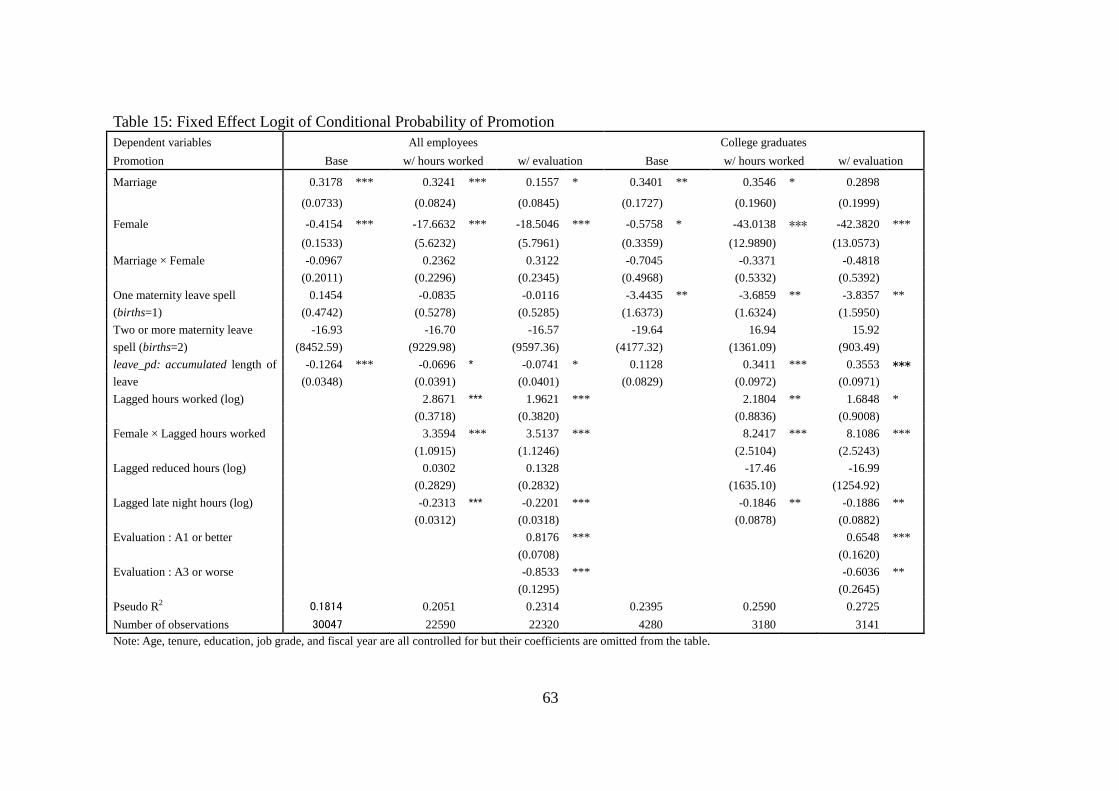
63

Table 15: Fixed Effect Logit of Conditional Probability of Promotion Dependent variables All employees College graduates Promotion Base w/ hours worked w/ evaluation Base w/ hours worked w/ evaluation

Marriage 0.3178 *** 0.3241 *** 0.1557 * 0.3401 ** 0.3546 * 0.2898

(0.0733)

(0.0824)

(0.0845)

(0.1727)

(0.1960)

(0.1999)

Female -0.4154 *** -17.6632 *** -18.5046 *** -0.5758 * -43.0138 *** -42.3820 *** (0.1533)

(5.6232)

(5.7961)

(0.3359)

(12.9890)

(13.0573)

Marriage × Female -0.0967

0.2362

0.3122

-0.7045

-0.3371

-0.4818

(0.2011)

(0.2296)

(0.2345)

(0.4968)

(0.5332)

(0.5392)

One maternity leave spell (births=1)

0.1454

-0.0835

-0.0116

-3.4435 ** -3.6859 ** -3.8357 ** (0.4742)

(0.5278)

(0.5285)

(1.6373)

(1.6324)

(1.5950)

Two or more maternity leave spell (births=2)

-16.93

-16.70

-16.57

-19.64

16.94

15.92

(8452.59)

(9229.98)

(9597.36)

(4177.32)

(1361.09)

(903.49)

leave_pd: accumulated length of leave

-0.1264 *** -0.0696 * -0.0741 * 0.1128

0.3411 *** 0.3553 ***

(0.0348)

(0.0391)

(0.0401)

(0.0829)

(0.0972)

(0.0971)

Lagged hours worked (log)

2.8671 *** 1.9621 ***

2.1804 ** 1.6848 *

(0.3718)

(0.3820)

(0.8836)

(0.9008)

Female × Lagged hours worked

3.3594 *** 3.5137 ***

8.2417 *** 8.1086 ***

(1.0915)

(1.1246)

(2.5104)

(2.5243)

Lagged reduced hours (log)

0.0302

0.1328

-17.46

-16.99

(0.2829)

(0.2832)

(1635.10)

(1254.92)

Lagged late night hours (log)

-0.2313 *** -0.2201 ***

-0.1846 ** -0.1886 **

(0.0312)

(0.0318)

(0.0878)

(0.0882)

Evaluation : A1 or better

0.8176 ***

0.6548 ***

(0.0708)

(0.1620)

Evaluation : A3 or worse

-0.8533 ***

-0.6036 **

(0.1295)

(0.2645)

Pseudo R2 0.1814

0.2051

0.2314

0.2395

0.2590

0.2725

Number of observations 30047 22590 22320 4280 3180 3141

Note: Age, tenure, education, job grade, and fiscal year are all controlled for but their coefficients are omitted from the table.

64

Figure 4 Predicted Odds of Promotion − Dotted lines indicate 95% confidence interval. − Figures in the tables show distribution by hours worked (4-1) All employees

43.3% 22.6% 12.7% 9.1% 5.3% 5.3% 1.8% 6.8% 15.0% 15.2% 21.2% 16.9% 15.1% 9.9%

(4-2) College graduate employees

30.2% 20.9% 15.4% 14.5% 6.2% 8.8% 4.0%

7.2% 20.9% 12.6% 18.1% 15.2% 14.8% 11.3%

0%

2%

4%

6%

8%

10%

12%

14%

16%

18%

20%

<1800 <1900 <2000 <2100 <2200 <2400 ³2400

0%

5%

10%

15%

20%

25%

30%

<1800 <1900 <2000 <2100 <2200 <2400 ³2400

Female

Female

Female

Male

Male

Male

Female Male

65

Table 16 Ordered Logit Estimation of Evaluation Dependent variables All employees College graduates

Evaluation Base w/ leave history & hours worked Base w/ leave history

& hours worked Marriage -0.6032 *** -0.6190 *** -0.5835 *** -0.5645 *** (0.0440) (0.0476) (0.0953) (0.1041) Female -0.2773 *** -0.2568 *** 0.0195 -0.0725 (0.0836) (0.0910) (0.1446) (0.1552) Marriage × Female 0.7722 *** 0.2527 ** 0.3275 -0.0795 (0.1062) (0.1270) (0.2172) (0.2431) Ph.D. 0.5208 *** 0.5529 *** (0.1220) (0.1397) MS/MA 0.4686 *** 0.5028 *** (0.0651) (0.0704) BS/BA 0.2749 *** 0.3011 *** (0.0509) (0.0553) Technical College 0.1386 * 0.2477 *** (0.0724) (0.0776) 2-year college -0.1578 -0.1364 (0.1043) (0.1117) One maternity leave spell (births=1)

0.2994 * 0.2894 (0.1694) (0.4471)

Two or more maternity leave spells (births=2)

-0.0932 1.1006 (0.3279) (1.1874)

leave_pd: accumulated length of leave

0.0048 -0.0094 (0.0103) (0.0291)

Hours worked (log) -2.2148 *** -1.7047 *** (0.1742) (0.3363) Reduced hours (log) 0.1508 ** 0.4257 *** (0.0615) (0.1560) Late night hours (log) 0.0921 *** (0.0147) Working in the HQ 0.0553 -0.0021 0.0751 -0.0162 (0.0462) (0.0508) (0.0773) (0.0847) Control for age and tenure Yes Yes Yes Yes Control for school ranking No No Yes Yes Control for job grade Yes Yes Yes Yes Control for fiscal year Yes Yes Yes Yes Pseudo R2 0.0478 0.0533 0.0486 0.0460 Number of observations 43023 34453 8871 7220