dynamics of rotors in complex structures - intes of rotors in complex structures n ... the governing...

Dynamics of rotors in complex structures

N. Wagner, R. Helfrich

INTES GmbH, Stuttgart, Germanywww.intes.de; [email protected]

Summary:

Rotating parts can be found in many mechanical products likein vehicles, airplanes, ships, machine tools. Becauserotors are never perfect, imbalances are generating vibrations which not only excite the rotor itself but also otherjoint non-rotating parts. This coupling of rotating and non-rotating parts is an important point for virtual productdevelopment of parts with rotors.

First, the principles of modeling and analysis of rotors arerevisited and usual post-processing features of rotoranalysis results are shown. Second, an example for a joint structure with rotating and non-rotating parts is usedto demonstrate the coupling effect. In particular, sound radiation from non-rotating parts due to imbalances of therotor will be considered.

NAFEMS World Congress:June 9 - 12, 2013, Salzburg, Austria

– 1–

1 Introduction

Finite element technique has become a popular tool in rotordynamic analysis.

Dynamic studies of rotating machines are generally performed using, on the one hand, beam element models[11, 16] representing the position of the rotating shaft and, on the other hand, three-dimensional solid rotor-statormodels [8, 13, 14]. Axisymmetric models are used by [11]. A specific advantage of solid models is the inclusionof stress stiffening, spin softening, and temperature effects in the rotor dynamics analysis. Nowadays CAD modelsof rotors becoming more and more detailed. The tedious and time-consuming task of building equivalent beammodels is omitted by using solid models.

Rotor lateral vibration (sometimes called transverse or flexural vibration) is perpendicular to the axis of the rotorand is the largest vibration component in most high-speed machinery [10]. Understanding and controlling thislateral vibration is important because excessive lateral vibrations leads to bearing wear and, ultimately, failure. Inextreme cases, lateral vibration also can cause the rotating parts of a machine to come into contact with stationaryparts, with potentially disastrous consequences [10, 12].

All FEM computations are carried out in PERMAS [1]. PERMAS specific commands are highlighted by a pre-ceding dollar sign and capital letters in the subsequent sections.

2 Governing Equations

Only linearized systems are considered here, i.e. only small variations of the rotational velocity is possible.Rotating systems may be processed in a stationary referenceframe as well as a rotating reference frame.

In the following, we will focus on an inertial reference frame. The additional matrices due to rotating parts mustbe taken into account and are requested by a so-called $ADDMATRIX data block within the $SYSTEM block.

The complex eigenfrequencies of a rotor on fixed supports aredetermined. The structure is described with respectto a fixed reference frame, i.e. shaft and discs rotate with a constant rotational speed, whereas the bearings aresupported and fixed to ground. All displacements, frequencies etc. refer to the fixed coordinate system. At oneend, the rotation is suppressed to represent a drive with constant rotational speed.

The first computation step is a static analysis for the basic model to determine the stress distribution under cen-trifugal loads. It is a prerequisite for the calculation of the geometric stiffness matrixKg.

The next step is the calculation of real eigenmodesX =[x1 . . .xr

], including geometric and convective

stiffness matrices:

MX = (K +Kg +Kc)X Λ, Λ =

λ1

.. .λr

. (1)

The governing equations of motion that describes a rotor system in a stationary reference frame is given by

M u+ (D +Db(Ω) +G) u+ (K +Kb(Ω) +Kg +Kc) u = R(t), (2)

whereM denotes the mass matrix,D viscous damping matrix,Db(Ω) speed-dependent bearing viscous dampingmatrix, G gyroscopic matrix,Kc convective stiffness matrix,Kg geometric stiffness matrix,Kb(Ω) speed-dependent bearing stiffness matrix and

Material damping iH of the stator is replaced by an equivalent viscous damping inthe time-domain.

Including convective stiffness requires the use of a consistent mass matrix, which is the default formulation begin-ning with version 14.

The equations of motion (2) are transformed into modal spaceby means of

u = X η (3)

Additional pseudo mode shapes may be added to enrich the modal space. This is realized by $ADDMODES.

M η +(D + G

)η +

(K + Kg + Kc

)η = R(t) (4)


– 2–

By introducingζ = η the second order form (4) is transformed into a state-space form:

[M O

O I

] [ζ

η

]+

[D + Db + G K + Kg + Kc

−I O

] [ζ

η

]=

[R(t)0

](5)

To analyse rotating models two different coordinate systems can be used in PERMAS, stationary and rotating.By using a stationary reference frame the model can have bothrotating parts and stationary parts. However, therotation parts have to be axisymmetric. Moreover differentcomponents can rotate with different rotational speeds.A stationary reference frame is activated by

$ADDMATRIX

GEOSTIFF CONVSTIFF GYRO

The rotational speed is defined in the loading definition of a static pre-run by $INERTIA ROTATION. Additionalmatrices are build for that reference speed.

The modelling of a rotating machine requires a skew-symmetric pseudo-damping matrix named gyroscopic ma-trix. The particular form of the matrix makes complex eigenmodes appear, forward modes having increasingfrequencies and backward modes having decreasing frequencies.

Critical speeds, stability and unbalance response were evaluated in the operating speed range.

2.1 Bearings

To a greater or lesser extent, all bearings are flexible and all bearings absorb energy. For most types of bearing, theload-deflection relationship is nonlinear. Furthermore, load deflection relationships are often a function of shaftspeed. Speed-dependent bearings are idealized by CONTROL6elements and multipoint constraints of type $MPCWLSCON.

2.2 Damping

Identical damping specifications lead to different effectsin fixed or co-rotating reference systems. In an inertialreference frame material damping is not suitable for rotating parts, whereas modal damping represents any kindof external damping. Discrete damping elements can be used for modelling damping in bearings.

2.3 Unbalance

In all rotating machinery, some degree of mass unbalance is always present. The unbalance load acts as a harmonicload in an inertial frame, i.e. [

Fx

Fy

]= meΩ2

[cosΩtsinΩt

]. (6)

The balance quality grades for various groups of representative rigid rotors can be found in ISO 1940/1 and isdefined as the product of a specific unbalancee in mm and the angular velocityΩ in rad/s of the rotor at maximumoperating speed:

G = eΩ. (7)

3 Examples

3.1 Gas Turbine

The first example is taken from the literature [9]. However wewill use a solid model instead of a Timoshenkobeam model. The solid model consists of 48372 hexahedra and 1000 pentahedra elements. Fig. 1 shows the meshof the rotor model. The front and rear bearing are located atx = 0.04 m andx = 0.7 m, respectively. The rotorconsists of 6 discs and a hollow shaft (l = 0.78 m). Details concerning the physical and geometrical data can befound in [9].


– 3–

VisPER (Visual PERMAS) is used for model validation and postprocessing tasks [3]. Medina is applied to generatethe finite element mesh [5].

Fig. 1: Simplified rotor model of a gas turbine

Fig. 2 illustrates the characteristic of the frequency-dependent isotropic bearings.

Fig. 2: Frequency-dependent coefficients of the bearings


– 4–

3.1.1 Strain energy distribution

The strain energy distribution of the different parts of therotor is illustrated in Fig. 3. Each colum represents aneigenfrequency of the rotating system. Bending modes appear pairwise due to the symmetry of the rotor-bearingsystem. The third and sixth column represent torsional modes shapes. The first two bending modes are dominatedby the rear bearing, whereas the front bearing participatesin modes 4,5 and 7,8 respectively. Modes 11 and 12exhibit axial modes of the shaft and discs. The elastic discsmake a contribution to the strain energy density athigher modes, while the lower modes are dominated by the hollow shaft.

Fig. 3: Strain energy distribution

3.1.2 Campbell Diagram

In order to get the relation between eigenfrequencies and rotational speed an automatic procedure called $MODALROTATING is available which directly generates all eigencurves. A mode tracking algorithm is implemented inorder to sort the complex eigenvalues.

The Campbell diagram is depicted in Fig. 5. Solid lines denotes the eigencurves computed by PERMAS whilethe dash-dot lines corresponds to the beam model studied in [9]. Torsional modes are not present in the beammodel. Besides the 3rd forward whirl all eigencurves are in good accordance with the results of the beam model.However, they share the feature of a strong variation with increasing rotor speed. The deviations within theCampbell diagram can be explained by the different modelingapproaches. The beam model tends to be stifferthan the solid model especially for higher modes.

The first critical speed corresponding to the first forward whirl (FW) is at 51 Hz and a second critical speed relatedto the second forward whirl is atf = 150 [Hz].

Nelson [15] showed that the backward mode vector is orthogonal to the unbalance vector and, as such, energy can-not be fed into the backward whirl. Therefore, critical speeds are restricted to forward whirl in case of symmetricrotors.

In order to judge the stability, the equivalent damping ratio

ξj = −δj√

δ2j + ω2

j

(8)

is evaluated. The system is stable, ifξj > 0∀ j. This condition is obviously satisfied here (s. Fig 4).


– 5–

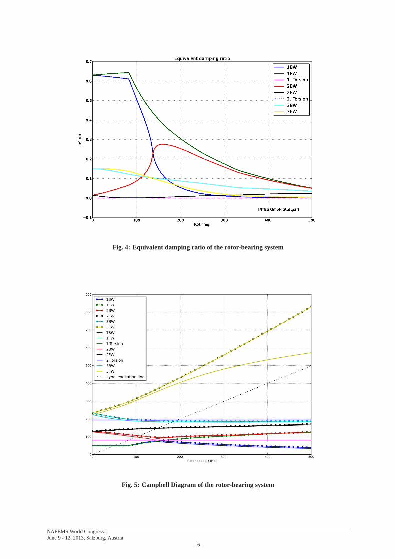
Fig. 4: Equivalent damping ratio of the rotor-bearing system

Fig. 5: Campbell Diagram of the rotor-bearing system


– 6–

3.1.3 Unbalance

A mass unbalance of10−4 kg m situated at the single disc at node 21 of the finite elementmodel is applied inthe numerical analyses. Fig. 6 illustrates the amplitudes due to a mass unbalance at different nodes. The peakcorresponding to the first critical speed is missing, since the damping of the rear bearing (Fig. 2) attenuates theresponse.

Fig. 6: Unbalance responses at certain nodes of the rotor-bearing system

The dynamic reaction forces of the bearings are depicted in Fig. 7

0 100 200 300 400 500Frequency f [Hz]

10-3

10-2

10-1

100

101

102

103

104

Bearing force F [N]

FrontRear

Fig. 7: Dynamic bearing forces


– 7–

3.2 Bench grinder

A bench grinder is a type of benchtop grinding machine used todrive abrasive wheels [7]. Depending on the gradeof the grinding wheel it may be used for sharpening cutting tools such as lathe tools or drill bits.

Alternatively it may be used to roughly shape metal prior to welding or fitting. Grinding wheels designed for steelshould not be used for grinding softer metals, like aluminium. The soft metal gets lodged in the pores of the wheeland expand with the heat of grinding. This can dislodge pieces of the grinding wheel.

The CAD model of the bench grinder is available through Grabcad [6].

Fig. 8: Bench grinder: Diameter of grinding wheelD = 123mm

It is an established fact that the casing has an effect on the dynamics of a rotor. Therefore, the interaction betweenth dynamics of the rotor with that of the casing is an essential aspect of the rotor dynamics. Therefore, all analysesare performed for the coupled system including the non-rotating and rotating part, respectively.

3.2.1 Speed-dependent bearings

A diagonal stiffness matrix

Kb(Ω) = diag[f2001(Ω) f2002(Ω) f2002(Ω) 0 105 105

](9)

is assumed for the bearings - hence cross coupling effects are neglected. The functionsf2001.f2002 in equation (9)are illustrated in Fig. 9.


– 8–

0 100 200 300 400 500Rotor speed [Hz]

5000

10000

15000

20000

25000

30000Stiffness k [N/m

m]

f2001

f2002

Fig. 9: Speed-dependent bearing stiffness

In addition a constant viscous damping matrix

Db = diag[0.5 1.0 1.0 1.e− 5 2.0 2.0

](10)

is used within the simulations.

The unbalance forces are assumed to be concentrated forces at the center of gravity of each grinding wheel.

3.2.2 Centrifugal load

The displacement under centrifugal loads is illustrated inFig. 10. The static pre-run is necessary to compute theadditional matrices due to rotation.

Fig. 10: Displacement field due to a centrifugal load


– 9–

The Campbell diagram is shown in Fig. 11

0 50 100 150 200 250 300 350 400Rotor speed

0

50

100

150

200

250

300

350

400Fr

equency

[Hz]

INTES GmbH Stuttgart

Mode1Mode3Mode5Mode7Mode9Mode11Mode13Mode15Mode17

Fig. 11: Campbell diagram of the bench grinder

3.2.3 Sound radiation

Sound radiation power (densities) may be computed after an eigenvalue analysis, a frequency response or a timehistory analysis in PERMAS. The results are generated for all shell, membrane, so-called LOADA and FSINTAelements. The sound radiation power density is proportional to

v2 =1

A

∫v2ndA, (11)

wherevn is the normal velocity of the vibrating surface. The result is the mean square value of the element velocitynormal to the element surface.

The unbalance response of the bench grinder is presented at 50 cycles/s (s. Fig 12).

Fig. 12: Sound radiation power density atf = 50.0 [Hz]


– 10–

4 Conclusions

A complete rotor dynamic analysis was successfully performed and verified by an example from the literature.Typical results such as Campbell diagram, dynamic bearing forces due to an unbalance load, and critical speedswere evaluated. The second example addressed the rotor-stator interaction of a bench grinder. In addition thesound radiation power is computed for rotating and non-rotating parts of the structure.

Possible extensions of the presented material include:

• Design of lightweight rotating structures at high speeds requires a deep knowledge of rotordynamics toavoid excessive vibration in the operating speed range. Forthis reason it becomes obvious to use optimiza-tion techniques [17] in order to reduces stresses, displacements, etc. For this purpose PERMAS providesdifferent modules such as topology, sizing and shape optimization. Various design constraints like $DCON-STRAINT WEIGHT, FREQ, CAMPBELL, CFREQ, NPSTRESS, ELSTRESS are available to optimize thestructure with regard to the above-mentioned constraints without the need to integrate an external optimizerin the process chain. Furthermore a positioning optimization is disposable.

• Further aspects such as critical speed maps, where the critical speeds are plotted as a function of the bearingstiffness in a semi-logarithmic manner, are important for abetter understanding of rotor-bearing systems.

5 Acknowledgment

The authors would like to thank Dr. João C. Menezes and Dr. Geraldo Creci Filho for providing the Campbelldiagram of the first example.

References

[1] PERMAS Version 14: Users’ Reference Manual, INTES Publication No. 450, Stuttgart, 2012.

[2] PERMAS Version 14: Examples Manual, INTES Publication No. 550, Stuttgart, 2012.

[3] Visper Version 3.1.005: Visper Users Manual, INTES Publication No. 470, Stuttgart, 2012.

[4] PERMAS Product Description Version 14, INTES, Stuttgart, 2012,http://www.intes.de/kategorie_unternehmen/publikationen

[5] Medina FEM Pre- and Post-Processing, T-Systems International GmbH,http://servicenet.t-systems.com/medina

[6] Grabcadhttp://grabcad.com/library/bench-grinder

[7] Bench grinderhttp://en.wikipedia.org/wiki/Bench_grinder

[8] D. Combescure, A. Lazarus:Refined finite element modelling for the vibration of large rotating machines: Applicationsto the gas turbine modular helium reactor power conversion unit, Journal of Sound and Vibration, Vol. 318, pp. 1262–1280, (2008).

[9] G. Creci, J. C. Menezes, J. R. Barbosa, J. A. Corra:Rotordynamic analysis of a 5-kilonewton thrust gas turbine byconsidering bearing dynamics, Journal of Propulsion and Power, Vol. 27, pp. 330–336, 2011.

[10] M. I. Friswell, J. E. T. Penny, S. D. Garvey, A. W. Lees:Dynamics of rotating machines, Cambridge University Press,2010.

[11] M. Geradin, N. Kill: A new approach to finite element modelling of flexible rotors, Eng. Comput., Vol. 1, pp. 52–64,1984.

[12] G. Jacquet-Richardet, M. Torkhani, P. Cartraud, F. Thouverez, T. Nouri Baranger, M. Herran, C. Gibert, S. Baquet,P. Almeida, L. Peletan:Rotor to stator contacts in turbomachines. Review and application, Mechanical Systems andSignal Processing, in press, (2013).

[13] A. Nandi, S. Neogy:Modelling of rotors with three-dimensional solid finite elements, Journal of Strain Energy, Vol. 36,pp. 359–371, 2001.

[14] A. Nandi: On computation of response of a rotor in deformed configuration using three-dimensional finite elements,Communications in Numerical Methods in Engineering, Vol. 19, pp. 179–195, 2003.

[15] F. C. Nelson:Rotor dynamics without equations, International Journal of COMADEM, Vol. 10, pp. 2–10, 2007.

[16] H. D. Nelson:A finite rotating shaft element using Timshenko beam theory, Journal of Mechanical Design, Vol. 102, pp.793-803, 1980.

[17] A. O. Pugachev, A. V. Sheremetyev, V. V. Tykhominov, I. D. Timchenko: Gradient-based optimization of a turbo-prop rotor system with constraints on stresses and natural frequencies, 51st AIAA/ASME/ASCE/AHS/ASC Structures,Structural Dynamics, and Materials Conference, 12-15 April 2010, Orlando, Florida.

[18] M. B. Wagner, A. Younan, P. Allaire, R. Cogill:Model reduction methods for rotor dynamic analysis: A survey andreview, International Journal of Rotating Machinery, Vol. , 2010.


– 11–

[19] PERMAS Version 14: Rotierende Systemehttp://www.intes.de/kategorie_permas/anwendungen/rotierende_systeme


– 12–

dynamics of rotors in complex structures - intes of rotors in complex structures n ... the governing...

Documents