6

Dynamics of Jupiter's Atmosphere

Andrew P. Ingersoll California Institute of Technology

Timothy E. Dowling University of Louisville

Peter J. Gierasch Cornell University

Glenn S. Orton Jet Propulsion Laboratory, California Institute of Technology

Peter L. Read Oxford University

Agustin Sanchez-Lavega Universidad del Pais Vasco, Spain

Adam P. Showman University of Arizona

Amy A. Simon-Miller NASA Goddard Space Flight Center

Ashwin R. Vasavada Jet Propulsion Laboratory, California Institute of Technology

6.1 INTRODUCTION

Giant planet atmospheres provided many of the surprises and remarkable discoveries of planetary exploration during the past few decades. Studying Jupiter's atmosphere and comparing it with Earth's gives us critical insight and a broad understanding of how atmospheres work that could not be obtained by studying Earth alone.

Jupiter has half a dozen eastward jet streams in each hemisphere. On average, Earth has only one in each hemi­sphere. Jupiter has weather patterns ("storms") that last for centuries. Earth has stationary weather patterns fixed to the topography, but the average lifetime of a traveling storm is rvl week. Jupiter has no topography, i.e., no con­tinents or oceans; its atmosphere merges smoothly with the planet's fluid interior. Absorbed sunlight (power per unit area) at Jupiter is only 3.3% that at Earth, yet Jupiter's winds are 3-4 times stronger. The ratio of Jupiter's internal power to absorbed solar power is 0. 7. On Earth the ratio

is 2 x 10-4. Jupiter's hydrologic cycle is fundamentally dif­

ferent from Earth's because it has no ocean, but lightning

occurs on both planets. On Earth, electrical charge separa­tion is associated with falling ice and rain. On Jupiter, the separation mechanism is still to be determined.

The winds of Jupiter are only 1/3 as strong as those of Saturn and Neptune, and yet the other giant planets have less sunlight and less internal heat than Jupiter. Earth probably has the weakest winds of any planet, although its absorbed solar power per unit area is largest. All the gi­ant planets are banded. Even Uranus, whose rotation axis is tipped 98° relative to its orbit axis, exhibits banded cloud patterns and east-west (zonal) jets. All have long-lived storms, although Jupiter's Great Red Spot (GRS), which may be hundreds of years old, seems to be the oldest.

6 .1.1 Data Sets

Early astronomers, using small telescopes with their eyes as detectors, recorded the changing appearance of Jupiter's atmosphere. Their descriptive terms - belts and zones,

brown spots and red spots, plumes, barges, festoons, and streamers- are still used. Other terms- describing vorticity,

106 Ingersoll et al.

vertical motion, eddy fluxes, temperature gradients, cloud heights, and wind shear - have been added, bringing the study of Jupiter's atmospheric dynamics to a level similar to that of Earth during the pioneering clays of terrestrial meteorology several decades ago.

Jupiter has what is perhaps the most photogenic at­mosphere in the solar system. Most of the visible contrast arises from clouds in the 0. 7- to 1.5-bar range (see Chap­ter 5). The clouds come in different colors, and usually have texture on scales as small as a few tens of kilometers, which is comparable to thee-folding thickness (scale height) of the atmosphere. At this resolution, cloud tracking over a few hours yields wind estimates with errors of a few m s- 1

. In contrast, the winds around the GRS and many of the zonal jets exceed 100 m s- 1

. Winds are measured relative to Sys­tem III, a uniform rotation rate with period 9 h 55 m 29.71 s, which is defined by radio emissions that are presumably tied to the magnetic field and thus to the planet's interior.

Traditional Earth-based telescopic resolution is 3000 km, which is enough to image the major atmospheric fea­tures. Pioneers 10 and 11 improved on Earth-based res­olution, but Voyagers 1 and 2 provided a breakthrough. For cloud tracking, the most important data were the "ap­proach" movies that were recorded during the three months prior to each of the two encounters in March and July of 1979. The spacecraft obtained a view of each feature every "-' 10 hours as the resolution improved from 500 km to 60 km. Occasional views of selected features continued down to a resolution (pixel size) of rv5 km. The Voyager infrared spectrometer (IRIS) viewed the entire planet at a resolu­tion of several thousand kilometers and obtained spectra of all the major dynamical features. Galileo obtained less data than Voyager, but the imaging resolution, usually 25 km, and the wavelength coverage were better. In particular, the near-infrared response of the Galileo camera allowed imag­ing in the absorption bands of methane, from which one separates clouds at different altitudes. Cassini combined the high data rate of Voyager with the broad spectral coverage of Galileo, yielding a best resolution of 60 km (the Cassini data were still being analyzed at the time of this writing).

Ground-based telescopes and the Hubble Space Tele­scope (HST) provide a continuous record of Jupiter's cloud features at several-month intervals. These data document the major events and also the extreme steadiness of the atmosphere. Ground-based telescopes provide the highest spectral resolution. Several trace gases, which provide im­portant diagnostics of vertical motion, were discovered from the ground. Earth-based radio observations probe the deep atmosphere. The HST was essential during the collisions of Comet Shoemaker-Levy 9 with Jupiter in 1994. Besides recording the waves and debris from the collisions, the HST defined the prior dynamical state of the atmosphere.

The Galileo probe provided profiles of wind, tempera­ture, composition, clouds, and radiation as functions of pres­sure clown to the 22-bar level, but only at one point on the planet. Except at the Galileo probe site, these quantities are uncertain below the 1-bar level. The base of the water cloud is thought to lie at the 6- or 7-bar level, "-'75 km below the clouds that produce the visible contrast.

6.1.2 Scope of the Chapter and Role of Models

This chapter reviews the observations and theory of Jupiter's atmospheric dynamics. Sections 6.2 and 6.3 cover the banded structures and discrete features, respectively. Section 6.4 covers vertical structure and temperatures. Sec­tion 6.5 discusses lightning and models of moist convection. Section 6.6 reviews numerical models of the bands and zonal jets, and Section 6. 7 reviews numerical models of the dis­crete features. Finally, Section 6.8 provides a discussion of outstanding questions and how they might be answered. The chapter is aimed at a general planetary science audience, al­though some familiarity with atmospheric dynamics is help­ful for the modeling sections.

As in the terrestrial atmospheric sciences, validated nu­merical models are the key to understanding. Models of Jupiter's atmosphere tend to be less complex than models of Earth's atmosphere. They nevertheless contain much of the nonlinear physics associated with large-scale stratified flows in rotating systems. Ideally, the complexity of the models matches that of the observations, so that hypotheses can be tested cleanly. Some pure fluid dynamics models, e.g., of two-dimensional flows without viscosity, find their best applications on Jupiter and the other giant planets. Exam­ples include the Kida vortex model, the models of inverse cascades and beta-turbulence, and the statistical mechan­ical models of two-dimensional coherent structures. These models are discussed in Sections 6.6 and 6. 7.

Peek (1958) is the definitive book for early observa­tions of Jupiter's atmosphere. Gehrels (1976) is a collec­tion of chapters by various authors following the Pioneer encounters. Rogers (1995) is the modern equivalent of Peek. There are many review articles (Ingersoll1976b, Stone 1976, Williams 1985, Beebe et al. 1989, Ingersoll 1990, Marcus 1993, Gierasch and Conrath 1993, Dowling 1995a, Ingersoll et al. 1995). As an ensemble, the articles record the variance of expert opinion. As a time series, they record the progress that has been made and bring clarity to the remaining unan­swered questions.

For a point on the surface of an oblate planet, there are two definitions of latitude. Planetographic (PG) latitude is the elevation angle (relative to the equatorial plane) of the vector along the local vertical, and planetocentric (PC) lati­tude is the elevation angle (relative to the equatorial plane) of the vector from the planet's center. PG latitude is greater than PC latitude except at the equator and poles where they are equal. For Jupiter the maximum difference (4.16°) is at 46.6° PG latitude. Unless otherwise specified, we use PG latitudes in this chapter.

6.2 BANDED STRUCTURE

6.2.1 Belts and Zones

Jupiter's visible atmosphere is dominated by banded struc­tures (Figure 6.1). Traditionally, the white bands are called zones and the clark bands are called belts. The zonal jets (eastward and westward currents in the atmosphere) are strongest on the boundaries between the belts and zones (Figure 6.2). The zones are anticyclonic, which means they have an eastward jet on the poleward side and a westward jet on the equatorward side (in the reference frame of the planet,

Atmospheric Dynamics 107

Figure 6.1. Whole disk views of Jupiter. The left image is from Voyager 2 in Jlllle 1979. The right image is from Cassini in November 2000. At the time of going to press a colour version of this figure was available for download from http://www.cambridge.org/9780521035453.

an anticyclone rotates clockwise in the northern hemisphere and counterclockwise in the southern hemisphere). The belts are cyclonic, which means they rotate the opposite way. In an inertial frame, the rotation period varies with latitude in a range ±5 min on either side of the System III period. The major belts and some inertial rotation periods are labeled in Figure 6.3 (Peek 1958, Stone 1976). Individual features like the GRS tend to have the same sign of vorticity (sense of rotation) as the band in which they sit.

Jupiter is not bright orange or red in color, but more of a muted brown (Peek 1958, Simon-Miller et al. 2001a). The colors of the belts and zones vary with time. The origin of the colors and how they respond to the winds are un­certain. The major cloud constituents- ammonia, H2S, and water- are colorless, but elemental sulfur, phosphorus, and organic compounds could combine in trace amounts to form the muted colors.

The zones appear more uniform than the belts, partic­ularly in the northern hemisphere. In the zones the small­scale texture has low contrast. The large-scale features in the zones are generally steadier in time than those in the belts. The clouds in the zones generally extend to higher altitudes than those in the belts; the corresponding pressure differ­ence is a few hundred mbar. The gaseous ammonia abun­dance is higher in the zones, and the upper tropospheric tem­peratures are lower (Conrath and Gierasch 1986, Gierasch et al. 1986, Simon-Miller et al. 2001b). The darker belts have deeper clouds overall and more variation in cloud height. There are holes in the visible cloud deck (5-~m hot spots, Figure 6.4) that allow radiation to escape from the warmer layers below (Terrile and Westphal 1977, Ortiz et al. 1998); this radiation is most intense in a narrow wavelength region around 5 f.-LID where there are no gaseous absorption lines to impede it. The belts are the sites of initially small convec­tive events that sometimes grow to great heights and encir-

cle the entire planet (Beebe et al. 1989, Simon-Miller et al. 2001 b). Amateur and professional observers have recorded many such disturbances (e.g., Sanchez-Lavega et al. 1991, Sanchez-Lavega and Gomez 1996, Rogers 1995). Although the belt/zone boundaries align closely with the zonal jets, they do change in latitudinal extent and can recede or ex­tend beyond the cores of the jets (Beebe et al. 1989, Rogers 1995, Simon et al. 1998).

Imbedded in the zones are the major anticyclonic ovals like the GRS at 22.5°S, the White Ovals at 33°S, and smaller ovals at 41 °S, 34°N, 40°N, and 45°N PG latitudes. These ovals usually extend into the neighboring belt on the equa­torward side, and sometimes block it off. Then the belt be­comes a series of closed cyclonic cells, each one spanning the region between two anticyclonic ovals. Activity is great­est on the eastern end of each cyclonic cell, giving it the appearance of a turbulent wake extending off to the west of the anticyclonic oval. The best example is the South Equa­torial Belt (SEB), whose active part extends westward, just north of the GRS. Both the SEB and the North Equato­rial Belt (NEB) are sites of intense convective activity -lightning storms with high, thick clouds that double in area in less than half a day (Gierasch et al. 2000).

Jupiter's Equatorial Zone (EZ) lies between the east­ward jets at PG latitudes ±7°. The vorticity is anticyclonic (clockwise north of the equator and counterclockwise south of the equator), but the EZ is different from other zones. Methane band images that sound the upper troposphere re­veal an elevated haze that is thicker than that at neigh­boring latitudes. Visible band images reveal a bland cloud deck whose northern boundary is punctuated by a dozen 5-~m hot spots and plumes (Ortiz et al. 1998). The latter are high, thick clouds that trail off 10 000 km to the southwest. The plume heads are located just west of the hot spots and sometimes exhibit convective activity (Hunt et al. 1981).

108 Ingersoll et al.

40

........... 0' (!)

"0 20 .....___.

(!)

"0

.2 0 _j

.g 0

c (!) u 0

Q) -20 c 0

0::

-40

-100 -50 0 50 1 00 1 50 Eastward Velocity (m/sec)

Figure 6.2. Zonal winds vs. latitude in 1979 and 2000. The dashed line is from Voyager (Limaye 1986), and the solid line is from Cassini (Porco et al. 2003).

The Galileo probe entered on the southern edge of a hot spot at PG latitude 6.5°N (Orton et al. 1998). Neither plumes nor hot spots look like vortices; nevertheless non­zonal motions have been associated with them (Vasavada et al. 1998). Between 10-13 hot spot/plume pairs have been present since the Voyager era; however Pioneer images and historical records indicate that there may have been fewer in the past. The train of features translates to the east with a velocity of "'"'100m s- 1

. When this translation is removed from time-series images of Jupiter's equator, the growth, in­teractions, and decay of individual features over months to years become apparent (Ortiz et al. 1998). Cassini movies, Galileo probe results, and numerical simulations suggest that the features are probably a nonlinear wave traveling westward on a fast ( rv 160 m s - 1

) eastward jet (Showman and Dowling 2000).

The banded appearance at low latitudes gradually gives way at mid latitudes to a mottled appearance at high lat­itudes, which are dominated by closely spaced anticyclonic ovals and cyclonic features (Figure 6.5). Despite this mot­tled appearance, movies show that organized zonal mo-

~UPIJ.Q~i?. ..... §f.l.TS AND PERIODS OF ROTATION

rm

L-.-i------1--l-·---i----·-+---+---l-·--+---+---+---+--- ?.00 0 +'Xf +40"

Latitude

Figure 6.3. Jupiter's belts and zones and periods of rotation. The figure is from Stone (1976), who used data summarized by Peek (1958). Those data were derived from decades of Earth­based telescopic observations. The belts are NEB= North Equa­torial Belt, NTB =North Temperate Belt, N2 TB =North North Temperate Belt, etc., and similarly in the south. The zones are EZ = Equatorial Zone, NTrZ = North Tropical Zone, NTZ = North Temperate Zone, N2 TZ = North North Temperate Zone, etc., and similarly in the south. Periods are measured by track­ing features larger than rv 3000 km over time intervals of days or weeks. Short periods represent flow to the east relative to Sys­tem III, which is the 9 h 55 m 29.71 s period defined from radio frequency observations.

Figure 6.4. Whole disk image at a wavelength of 5 !J.m (Ortiz et al. 1998). The brightest areas, termed 5-!J.m hot spots, are holes in the visible cloud deck that reveal the warmer, deeper layers below. Maximum brightness temperatures sometimes exceed 273 K. The Galileo probe entered on the south edge of a hot spot at 6.5°N latitude.

tions extend to ±80° at least (Garcia-Melendo and Sanchez­Lavega 2001, Porco et al. 2003). Methane-band images dis­play prominent polar caps of elevated and thicker haze, pos­sibly maintained by auroral processes, with wave-like bound­aries (Rages et al. 1999, Sanchez-Lavega et al. 1998a, Chap­ter 5). Recent observations at ultraviolet wavelengths, which

are sensitive to stratospheric aerosols, reveal vortices and other features clearly distinct from those of the visible cloud deck and possibly associated with the auroral footprint (Vin­cent et al. 2000, Porco et al. 2003).

6.2.2 Changes in Appearance

Although Jupiter's banded appearance is quite stable, changes are visible in the Voyager and Cassini images ac­quired in 1979 and 2000, respectively (Figure 6.1). The equa­torial plumes were less well defined with respect to their surroundings in 2000 than they were in 1979, although they were present in roughly the same numbers. There was a re­versal in the north-to-south color gradient across the EZ as well (Simon-Miller et al. 2001b).

The NEB was more active around the time of the Cassini flyby. Dark material extended further to the north than in the Voyager era. Many active sites were visible, and possible brown barges (elongated cyclonic dark ovals not visible in Figure 6.1) were reported for the first time since the Voyager era (neither HST nor Galileo saw brown barges in the 1990 to mid-2000 time period). The North Temper­ate Belt (NTB, from 23° N to 31° N), showed more contrast with respect to the surrounding zones than in the Voyager era. None of these changes is particularly unusual. The belts and zones often change color or width. Good historical ac­counts of similar events are found in Peek (1958) and Rogers (1995). Detailed studies of recent disturbances in the SEB and NTB can be found in Sanchez-Lavega and Gomez (1996) and Sanchez-Lavega et al. (1991), respectively.

The GRS decreased in longitudinal extent and became much rounder in appearance during the 21 years between the Voyager and Cassini epochs. The three largest white ovals (not visible in the Cassini image) also decreased in size and eventually merged into a single vortex. The small ovals at 41 °S have not changed in appearance or number. Despite the slight differences in the ovals and belt/ zone appearance, the overall appearance of the planet and its major features in both frames of Figure 6.1 is remarkably unchanged.

6.2.3 Changes in Zonal Velocity

The velocities of Jupiter's zonal jets have been inferred from the translation of cloud features for hundreds of years (Peek 1958, Smith and Hunt 1976). Uncertainties arise from differ­ent instruments and wavelengths, inaccurate image naviga­tion, changes in the morphology of tracked cloud features, confusion of measurements by non-zonal circulations, and imperfect coupling of tracked features to the underlying zonal flow (e.g., Beebe et al. 1996). Nevertheless Voyager, Galileo, HST, and Cassini images have produced a 21-yr record of high-quality velocity measurements capable of re­vealing any decadal-scale variations greater than about 10 m s- 1 (Figure 6.2). The number and magnitude of Jupiter's jets have remained virtually unchanged, in spite of the pres­ence of turbulence, convection, uncertainty in altitude, and major changes in the brightness and width of the bands. The measured winds probably refer to levels in the 0. 7- to 1.0-bar range (Banfield et al. 1998).

Some minor variations in jet shape and speed have been

reproduced by several analyses, however, including the re­sults shown in Figure 6.2 (Limaye 1986, Vasavada et al. 1998,

Atmospheric Dynamics 109

Simon 1998, Garcia-Melendo et al. 2001, Porco et al. 2003). Between 1979 and 1995 the eastward jet at 23°N slowed from 180 m s-1 to 140 m s- 1 and then remained constant. The westward jet at 30°N and the jets between 40°N and 55°N also show significant ( 10-20 m s - 1

) changes and small shifts in latitude.

6.2.4 Two Hypotheses about the Banded Structure

Jupiter's large-scale winds are in approximate geostrophic balance; therefore anticyclones are high-pressure centers and cyclones are low-pressure centers. Warm-core features (warmer than their surroundings at the same pressure level) become more anticyclonic with altitude because pressure de­creases with altitude more slowly when the air is warm than when it is cold. By the same token, cold-core features be­come more cyclonic with altitude. Thus in the Earth's atmo­sphere, a warm-core feature like a hurricane changes from strongly cyclonic at low altitude to weakly anticyclonic at high altitude. And in the Earth's ocean, warm-core features may be weakly cyclonic or anticyclonic at depth, but they become strongly anticyclonic at the ocean surface. These are examples of a quantitative relation between wind shear and horizontal temperature gradient called the thermal wind equation (e.g., Pedlosky 1987).

For Jupiter, the traditional view (Hess and Panofsky 1951, Ingersoll and Cuzzi 1969) is that the winds are weak in the deep atmosphere as in the deep oceans; in other words, the winds that we see are shallow. This implies that the zones and anticyclonic ovals are warm-core features - the air between the deep "level of no motion" and the surface on which the winds are measured is warmer than the sur­roundings. Since warm air tends to rise and cold air tends to sink, it is natural to assume that the air in the zones is slowly rising and the air in the belts is slowly sinking. And since clouds tend to form on updrafts, this view seems to be consistent with the observation that the visible cloud deck is higher in the zones (and in the anticyclonic ovals) and lower in the belts. This view also seems to be consistent with the observation that the 5-~m hot spots, which are holes in the visible cloud deck, are concentrated in the belts (Terrile and Westphal 1977).

An alternate view (Busse 1976) is that the winds are just as strong in the deep atmosphere as they are in the visible cloud deck. If the fluid is barotropic, meaning that temperature is constant at constant pressure, the zonal jets would be the surface manifestation of differentially rotating cylinders concentric with the planet's rotation axis (Poincare 1910). The fluid would then move in columns, according to the so-called Taylor-Proudman theorem (e.g., Pedlosky 1987). On the other hand, if the fluid is baroclinic, mean­ing that temperature varies at constant pressure, the winds would not obey the Taylor-Proudman theorem and the fluid would not move in columns. Distinguishing between these two extremes, shallow vs. deep, requires knowledge of winds and temperatures in the deep atmosphere.

6.2.5 Evidence of Upwelling and Downwelling

Large-scale vertical velocities are estimated to be "'10-3 m s- 1

, which is too small to be measured directly. Departures

110 Ingersoll et al.

Figure 6.5. Polar views of Jupiter. Images from different longitudes were map projected to show, from a viewpoint directly over the pole all the features in sunlight at the same time. Latitude varies linearly with radial distance in the image, from 0° in the corners to 90° in the center. (Left) South pole in 1979 from Voyager. (Right) North pole in 2000 from Cassini.

from chemical and thermal equilibrium provide indirect ev­idence of vertical velocity when the equilibrium state is a function of altitude. We consider four examples. The first involves the fraction of H2 molecules in the two possible spin states, ortho and para. The equilibrium para fraction decreases with depth due to the increase in temperature, so a para fraction below the equilibrium value is a sign of upward motion. Second, a stably stratified atmosphere is one in which the potential temperature (or equivalently, the entropy) increases with height; therefore rising air tends to have low potential temperature and sinking air tends to have high potential temperature. It follows that when there are no other heat sources, low and high temperatures mean up­welling and downwelling, respectively. Third, ammonia con­denses and precipitates in the upper troposphere, so high ammonia abundance is generally a sign of upwelling. Fourth, clouds form on updrafts, so increased cloud optical thickness is generally a sign of upwelling.

The Voyager IRIS spectra allow simultaneous determi­nation of the ortho-para ratio, the temperature, the ammo­nia concentration, and cloud optical depths at two differ­ent wavelengths (5 and 45 J-lm), all with spatial resolution of a few thousand km over most of the planet. The tem­perature and para fraction refer to pressure levels of a few hundred mbar; the 45-J..lm cloud optical depth and the am­monia concentration refer to levels between 1 bar and space; and the 5- J-lm optical depth refers to levels between a few bars and space (Conrath and G ierasch 1986). An orderly pattern related to the zonal mean jets emerges from these measurements (Gierasch et al. 1986). Upper tropospheric temperatures are higher over the belts than over the zones, implying that the zones lose their anticyclonic vorticity and the belts lose their cyclonic vorticity as altitude increases,

i.e., the winds get weaker with altitude. Figure 6.6 compares the thermal wind shear 8uj8z, computed from the measured temperature gradient 8T / 8y, with the mean zonal wind u measured by cloud tracking, where y and z are the north­ward and upward coordinates, respectively. This decay of the zonal winds with altitude takes place over two or three scale heights. Cloud optical depths and ammonia abundance are displayed in Figure 6.7, and a ground-based 5-J..lm image is shown in Figure 6.4 (Orton et al. 1996, 1998). Regions of low 5-1-1m optical depth appear bright because they al­low thermal radiation from below to escape. The belts are regions of low optical depth and low ammonia abundance. The inference is that the air in the belts is sinking, at least within the upper troposphere (from 0.1 to 0.5 bars). Under this interpretation, the mean meridional motions (longitu­dinally averaged motions in the vertical and north-south directions) agree with the traditional view of zones as sites of upwelling and belts as sites of downwelling.

The temperatures of the upper troposphere (warm belts, cold zones) are opposite to those postulated for the lower troposphere according to the traditional view based on a level of no motion below the visible cloud deck. Yet in both cases one infers rising motion in the zones and sink­ing motion in the belts. The difference is that in the upper troposphere there are no obvious heat sources that would make the belts warmer - one has to invoke downwelling. In the lower troposphere one can invoke latent heat to keep the zones warmer (Ingersoll and Cuzzi 1969, Barcilon and Gierasch 1970).

The inferred circulation in the upper troposphere has hot air sinking and cold air rising. This is a thermally in­direct circulation, which stores potential energy and must be mechanically driven. Gierasch et al. (1986) and Conrath

45 150

- 30 l1 100 I'll Ci ,d

w -; 15 50

fi: ~ ~

-'jill 0 !

'Ill ::1

-50

-100

40 20 0 -20 PLANETOGRA.PHlC LATITUDE

Figure 6.6. Upper tropospheric ( I'V270 mbar) thermal wind shears compared with cloud-tracked wind velocities. The figure is from Gierasch et al. (1986), who computed the thermal wind shears from Voyager IRIS data. The cloud-tracked winds are from Limaye (1986) and refer to the I'VO. 7 bar level.

et al. (1990) argue that the mean zonal flow at cloud-top level provides the energy. That flow is subject to dissipation, which they parameterize as Rayleigh drag and Newtonian radiative damping. The dissipation causes the zonal winds to decay with altitude. The upwelling and downwelling above the clouds are part of a mean meridional overturning that balances the dissipative effects with Coriolis acceleration and vertical advection of potential temperature. Pirraglia (1989) and Orsolini and Leovy (1993a, 1993b) show that shear instability produces large-scale eddies that give the required decay of jets within the upper troposphere. The in­stabilities thus may be the physical process underlying the drag coefficient parameterization in the interpretation by Gierasch et al. (1986).

West et al. (1992) and Moreno and Sedano (1997) have calculated the residual mean meridional circulation (in the altitude-latitude plane) taking into account the belt-zone temperature differences as well as the absorbing aerosols that are found especially over the polar regions. Such aerosols increase the solar heating rates, and result in a hemisphere-wide circulation from 1 to 100 mbar. The belt­zone downwellings and upwellings were found to persist only up to the vicinity of the tropopause at rv100 mbar.

The hydrogen para fraction shows a large-scale gradient from a minimum near the equator to higher values near the poles, which is consistent with upwelling near the equator and sinking near the poles, but it does not show a systematic correlation with belts and zones the way the clouds and ammonia do (Gierasch et al. 1986). However these ortho­para data from the IRIS spectra refer to a higher level in the upper troposphere (a few hundred mbar) than do the cloud optical depths and the ammonia concentration, and thus may be diagnostic of a different dynamical regime.

Atmospheric Dynamics 111

2

~ «< !:; 1.5 C!

.3

~ Cl

..!::. s:: 0 ~ () .5 «<

.!::: ~ :z;

40 20 0 -20 -40 -60 PLANETOGRAPHIC LATITUDE

.a

I s ()

10 .4 N e ..

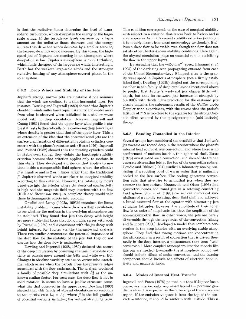
j

5 0 4 ID 0 e ..

0 60 40 20 0 -20 -60

PLANETOGRAPHIC LATITUDE

Figure 6. 7. Estimates of zonal mean ammonia concentration, 5-~-tm cloud optical depth (2050 cm-1 ), and 45-~-tm cloud optical depth (225 cm- 1 ) from Voyager IRIS spectra. Absolute values of these retrieved quantities are model dependent, but the relative values from latitude to latitude are reliable. Ammonia and 45- !-llll

cloud refer to levels between about 1 bar and space, and 5-~-tm cloud refers to levels between a few bars and space. All three quantities correlate well with continuum brightness in the visible (Gierasch et al. 1986).

6.3 DISCRETE FEATURES

6.3.1 Great Red Spot

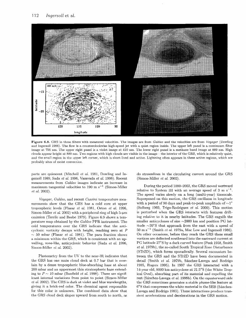
The GRS is probably the largest and oldest vortex in the atmospheres of the planets. Its oval shape appears in draw­ings from 1831, but it was tentatively first observed by J.P. Cassini and others from 1665 to 1713 (Rogers 1995). Mea­surements in 1880 showed that it had an east-west length of 39 000 km and a north-south width of 12 500 km. Its east­west length has decreased since then to its present 17 000 km (Beebe and Youngblood 1979, Rogers 1995, Simon-Miller et al. 2002). The GRS is an anticyclonic vortex (high pressure center) extending from 17°S to 27.5°S PG latitude. In 1979 it had a maximum velocity of 120m s- 1 along a peripheral collar and maximum relative vorticity ""'6 x 10-5 s- 1 , which

is about 1/3 the local planetary vorticity (vorticity due to the planet's rotation). As shown in Figure 6.8, its central

112 Ingersoll et al.

Figure 6.8. GRS in three filters with measured velocities. The images are from Galileo and the velocities are from Voyager (Dowling and Ingersoll 1988). The flow is a counterclockwise high-speed jet with a quiet region inside. The upper left panel is a continuum filter image at 756 nm. The upper right panel is a violet image at 410 nm. The lower right panel is a methane band image at 889 nm. High clouds appear bright at 889 nm. Two regions with high clouds are visible in the image- the interior of the GRS, which is relatively quiet, and the small region in the upper left corner, which is short-lived and active. Lightning often appears in these active regions, which are probably sites of moist convection.

parts are quiescent (Mitchell et al. 1981, Dowling and In­gersoll1989, Sada et al. 1996, Vasavada et al. 1998). Recent measurements from Galileo images indicate an increase in maximum tangential velocities to 190 m s- 1 (Simon-Miller et al. 2002).

Voyager, Galileo, and recent Cassini temperature mea­surements show that the CRS has a cold core at upper tropospheric levels (Flasar et al. 1981, Orton et al. 1996, Simon-Miller et al. 2002) with a peripheral ring of high 5-~-tm emission (Terrile and Beebe 1979). Figure 6.9 shows a tem­perature map obtained by the Galileo PPR instrument. The cold temperatures over the CRS indicate that the anti­cyclonic vorticity decays with height, reaching zero at P rv 50 mbar (Flasar et al. 1981). The para fraction shows a minimum within the CRS, which is consistent with an up­welling, zone-like, anticyclonic behavior (Sada et al. 1996, Simon-Miller et al. 2002).

Photometry from the UV to the near-IR indicates that the CRS has one main cloud deck at 0. 7 bar that is over­lain by a dense tropospheric blue-absorbing haze at about 200 mbar and an uppermost thin stratospheric haze extend­ing to P '"'-' 10 mbar (Banfield et al. 1998). There are signif­icant internal variations from point to point (Simon-Miller et al. 2002). The CRS is dark at violet and blue wavelengths, giving it a brick-red color. The chemical agent responsible for this color is unknown. The combined data show that the CRS cloud deck slopes upward from south to north, as

do streamlines in the circulating current around the CRS (Simon-Miller et al. 2002).

During the period 1880-2002, the CRS moved westward relative to System III with an average speed of 3 m s-1

.

The speed varies slowly on a long (multi-year) timescale. Superposed on this motion, the CRS oscillates in longitude with a period of 90 days and peak-to-peak amplitude of rv1 ° (Solberg 1969, Trigo-Rodriguez et al. 2000). This motion is perturbed when the CRS interacts with features drift­ing relative to it in nearby latitudes. The CRS engulfs the smaller anticyclones of size rv2000 km and position PC lat­itude rv20° S that approach from the east with a speed of 50 m s- 1 (Smith et al. 1979a, Mac Low and Ingersoll1986). On other occasions, before they reach the CRS these small vortices are deflected southward into the eastward current at PC latitude 27°S by a dark curved feature (Peek 1958, Smith et al. 1979b), the so-called South Tropical Zone Disturbance (STrZD), which forms sporadically. Several encounters be­tween the CRS and the STrZD have been documented in detail (Smith et al. 1979b, Sanchez-Lavega and Rodrigo 1985, Rogers 1995). In 1997 the CRS interacted with a 14-year old, 8000 km anticyclone at 21.5°S (the White Trop­ical Oval), absorbing part of its material and expelling the rest (Sanchez-Lavega et al. 1998b). On the equatorward side the CRS sometimes generates a stable plume-like feature at 6°S that compresses the white material in the SEB (Sanchez­Lavega and Rodrigo 1985). These interactions produce tran­sient accelerations and decelerations in the CRS motion.

Figure 6.9. Galileo PPR images of the GRS. The instrument records thermal emission from the gas in the upper troposphere, where the GRS is some 10 K colder than its surroundings. Since there are no radiative processes to account for these cooler tem­peratures, they are most likely due to upwelling of air with lower potential temperature.

6.3.2 White Ovals and Other Anticyclones

The GRS is the largest anticyclonic oval, but it is not unique. Most of the others are white, but some are red. White ovals are most conspicuous near PG latitudes 33°S and 41 °S but also occur near 17°N, 34°N and 40°N. The major diameter ranges from rv1000 km to over 5000 km. The ones at high latitudes are smaller and rounder than those at low latitudes (Mac Low and Ingersolll986, Morales-Juberfas et al. 2002a). The ratio of meridional to zonal extent approaches unity for the smallest ovals.

The three large white ovals at 33°S (termed BC, DE, and FA) formed when an anticyclonic, planet-encircling zone, the STZ, broke into three parts in 1939-40 (Peek 1958, Beebe et al. 1989, Rogers 1995). The ovals were similar in appearance and size (minor and major axes about 5000 and 10 000 km) but exhibited varied longitudinal drift rates (possibly correlated with latitude), spacing, and interactions with neighboring cyclonic features and the GRS. In the late 1990s, the eastward drift rate of oval BC slowed, causing the other ovals and intervening cyclonic features to pile up (com­press) on the westward side of BC (Simon et al. 1998). In early 1998, ground-based telescopes documented the merger of ovals BC and DE into a larger oval and possibly a small, cyclonic vortex (Sanchez-Lavega et al. 1999). Figure 6.10 shows BC and DE just before their merger, with a vastly re­duced cyclonic region squeezed in between them. Two years later the new oval merged with FA (Sanchez-Lavega et al. 2001) to form a single oval named BA.

Ovals form in several ways. Small ovals ( <1000 km) may form in updrafts (e.g., thunderstorm clusters) whose spreading motion produces anticyclonic vorticity. Ovals may

Atmospheric Dynamics 113

120 110 100 90 West Longitude

Figure 6.10. Galileo image of white ovals DE and BC shortly before their merger in 1998 (Vasavada et al. 1998). The ovals DE (left) and BC (right) are at 30°8 planetocentric latitude. They are anticyclones (counterclockwise in the southern hemisphere), and there is a cyclonic region between them. The eastward current at 32°8 flows south of DE and creates the white cloud on the west side of the cyclonic region. It then flows north, clockwise around the cyclonic region, and finally south of BC and out of the figure to the east. The white oval to the south did not participate in the merger.

also form when an anticyclonic zone breaks up, as the STZ did in 1939-40. Ovals disappear by merging and by getting stretched out in the large-scale shear flow. Observations and dynamical simulations suggest that within each mid-latitude zone ovals ingest or merge with others, suggesting that they would grow in size until one or a few dominate (Mac Low and Ingersoll 1986, Dowling and Ingersoll 1989). However, historical observations reveal that the semi-major axes of the largest white ovals and the GRS decrease over time (Simon­Miller et al. 2002) .

The anticyclonic rotation of the largest white ovals is well defined by their interior cloud texture. Tangential ve­locity increases approximately linearly with radial distance out to the visual boundary (Mitchell et al. 1981, Vasavada et al. 1998). Like the GRS, the white ovals are cold at up­per troposphere levels, even after mergers (Sanchez-Lavega et al. 1999, 2001). Their anticyclonic vorticity, the presence of colder upper-level temperatures, the observed increased altitude of overlying hazes, their bright, white coloration and dark halos all suggest moderate upwelling within white ovals (Conrath et al. 1981, Banfield et al. 1998). The GRS is distinguished from white ovals by its annular velocity struc­ture (surrounding an interior with little organized motion) and its coloration, which may indicate its greater ability to dredge and/ or confine trace species. Little red spots have occasionally been seen in the NTrZ, which is the northern counterpart of the STrZ where the GRS resides (Beebe and Hockey 1986). These small anticyclones have the same char­acteristic UV absorber that is present in the GRS but is not present in the belts.

6.3.3 Cyclonic Features

The cyclonic regions tend to be more spread out in the zonal direction than the anticyclonic ovals. They have a more chaotic, filamentary texture and tend to evolve more rapidly, though some survive for a few years. The cyclonic

114 Ingersoll et al.

regions contain a variety of organized morphologies that can be grouped in the following main categories (Smith et al. 1979a, 1979b, Mitchell et al. 1979, Morales-Juberias et al. 2002b): (1) filamentary turbulence related to the highest­speed jets in the SEB (west of the GRS) NEB and NTB· (2) organized folded filamentary regions (~ize 15,000 km, fil~ ament width ""'600 km); (3) elongated areas with contours closed by a ribbon-like feature; (4) discrete brown elongated ovals called "barges" (zonal extent ""'5000 km). Hatzes et al. (1981) measured the peripheral circulation of a barge and its shape oscillations. Like the cyclonic belts, the closed cy­clonic features are warmer than their surroundings at upper tropospheric levels, consistent with downwelling (Conrath et al. 1981).

At some latitudes the anticyclones "invade" the belt on their equatorward side and break it into a series of closed cyclonic cells. The cyclones alternate in longitude with the anticyclones, but they are offset from each other in latitude. This alternating pattern resembles a classic Karman vortex street (Youssef and Marcus 2003). In the laboratory and in nature, such configurations form in wakes behind blunt bod­ies and are stable to small perturbations. On Jupiter there is an asymmetry between the anticyclones and cyclones: The former are more compact; the latter are more elongated and have a more chaotic texture. For example, the 12 compact anticyclonic white ovals at 41 °S alternate in longitude with chaotic cyclonic patches that are a few degrees closer to the equator than the anticyclonic ovals (Figure 6.5, left). Such an asymmetry is not present in a classic vortex street but could arise in a rotating planetary atmosphere, perhaps be­cause the anticyclones are vertically thicker, which follows from the thermal wind equation, or perhaps because the cy­clonic belts are the sites of moist convection.

6.3.4 Eddy Momentum Flux

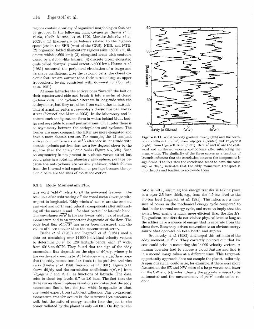
The word "eddy" refers to all the non-zonal features - the residuals after subtracting off the zonal mean (average with respect to longitude). Eddy winds u' and v' are the residual eastward and northward velocity components after subtract­ing off the means u and ii for that particular latitude band. The covariance pu'v' is the northward eddy flux of eastward momentum and is an important diagnostic of the flow. The eddy heat flux pCpv'T' has never been measured, and the values of v are smaller than the measurement error.

Beebe et al. (1980) and Ingersoll et al. (1981) used a data set containing over 14 000 individual velocity vectors to determine pu'v' for 120 latitude bands, each 1 o wide, from 60°8 to 60°N. They found that the sign of the eddy momentum flux depends on the sign of clujdy, where y is the northward coordinate. At latitudes where dujdy is posi­tive the eddy momentum flux tends to be positive, and vice versa (Beebe et al. 1980, Ingersoll et al. 1981). Figure 6.11 shows cluj ely and the correlation coefficients r( u', v') from Voyagers 1 and 2, all as functions of latitude. The data refer to cloud-top levels, 0.7 to 1.0 bars. The fact that the three curves show in-phase variations indicates that the eddy momentum flux is into the jets, which is opposite to what one would expect from turbulent diffusion. This up-gradient momentum transfer occurs in the terrestrial jet streams as well, but the ratio of energy transfer into the jets to the power radiated by the planet is only rvO.OOl. On Jupiter the

-6~2 0 du/dy (e-05/sec)

Figure 6.11. Zonal velocity gradient dujdy (left) and the corre­lation coefficient r( u', v') from Voyager 1 (center) and Voyager 2 (right), from Ingersoll et al. (1981). Here u' and v' are the east­ward and northward velocity components after subtracting the mean winds. The similarity of the three curves as a function of latitude indicates that the correlation between the components is significant. The fact that the correlation tends to have the same sign as dujdy indicates that the eddy momentum transport is into the jets and tending to accelerate them.

ratio is "-'0.1, assuming the energy transfer is taking place in a layer 2.5 bars thick, e.g., from the 0.5-bar level to the 3.0-bar level (Ingersoll et al. 1981). The ratios are a mea­sure of power in the mechanical energy cycle compared to that in the thermal energy cycle, and seem to imply that the jovian heat engine is much more efficient than the Earth's. Up-gradient transfers do not violate physical laws as long as the eddies have a source of energy that is separate from the shear flow. Buoyancy-driven convection is an obvious energy source that operates on both Earth and Jupiter.

Sromovsky et al. (1982) challenged this estimate of the eddy momentum flux. They correctly pointed out that bi­ases could arise in measuring the 14 000 velocity vectors. A human operator had to choose a cloud feature and find it in a second image taken at a different time. This target-of­opportunity approach does not sample the planet uniformly. A spurious signal could arise, for example, if there were more features on the SE and NW sides of a large vortex and fewer on the SW and NE sides. Clearly the procedure needs to be automated and the measurement of pu' v' needs to be re­done.

Atmospheric Dynamics 115

·- Pioneer 11 (inbound) - . ..._ Pioneer 10 - ·- Pioneer 11 (outbound) -

-SO -60 -40 -20 0 Latitude (deg}

60 80

Figure 6.12. Brightness temperature (right-hand ordinate) and intensity (left-hand ordinate) as a function of latitude for three different values of the emission angle cosine (Ingersoll et al. 1976) at wavelength bands centered at 20 and 45 ~-tm. The data are from Pioneer 10, which viewed the low latitudes, and Pioneer 11, which reached higher latitudes than any other spacecraft. Significant features of the curves include: (1) the agreement between Pioneers 10 and 11, (2) the lack of pronounced equator-to-pole contrasts, and (3) the higher brightness temperatures in belts (B) compared to zones (Z).

6.4 TEMPERATURES AND VERTICAL STRUCTURE

6.4.1 Global Temperature Variations

As shown in Figure 6.12, Jupiter has no appreciable equator­to-pole temperature gradient (Ingersoll et al. 1976, Pirraglia 1984). Except for variations on the scale of the belts and zones, the emitted infrared radiation is independent of lati­tude. This means that energy is being transported poleward, either in the atmosphere or in the interior, to make up for the extra sunlight absorbed at the equator. Ingersoll (1976a) and Ingersoll and Porco (1978) argued that Jupiter's inter­nal heat flux is diverted poleward by slightly lower polar temperatures at the top of the convection zone. Deep con­vection acts as a thermostat that maintains the equator and poles at essentially the same temperature. The fluid interior short-circuits the atmosphere, they argued, leaving it with no role in the global energy budget. Earth's oceans cannot do this because they are heated from above and are therefore dynamically less active than the atmosphere.

Jupiter has seasons despite its low 3° obliquity. Orton et al. (1994) found high-latitude temperature maxima two years after solstice at the 250-mbar level. The data cover one jovian year, from 1979 to 1993. This phase lag is consis­tent with the computed radiative time constant, which has a minimum of 4 x 107 s at the tropopause (Flasar 1989).

A prominent non-seasonal variation occurs in the Equa­torial Zone (EZ), whose 250-mbar temperature oscillates with a 4-year period and appears to be opposite in phase with the 20-mbar temperature (Orton et al. 1991, Chap­ter 7). Leovy et al. (1991) termed this the quasi-quadrennial oscillation (QQO) of Jupiter, and related it to upward­propagating, equatorially trapped waves in analogy with the quasi-biennial oscillation (QBO) of Earth's tropical atmo-

sphere. Using a numerical model, Friedson (1999) showed that large-scale equatorial waves are ineffective in driving

the oscillation but that forcing by small-scale gravity waves provides a better fit to the observations ( cf. Li and Read 2000).

Orton et al. (1994) also noted a large cooling at the 250-mbar level from 1985 to 1990 in a region between ap­proximately 15°N and 27°N (planetocentric), i.e., between the northern boundary of the NEB and the northern bound­ary of the North Temperate Belt (NTB). They estimated that if winds were steady at the cloud-top level near 60Q-700 mbar then a large cooling trend at the 250-mbar level recorded between 1985 and 1990 implied, through the ther­mal wind relationship, that the zonal wind decreased by at least 3 m s -l per terrestrial year.

6.4.2 Thermal Waves

The profiles of the Voyager radio occultation experiment (Lindal et al. 1981) show wave-like features (Figure 6.13), although Lindal et al. suggested that they could be the result of local particulate layers that absorb sunlight. The features have vertical length scales of rv 1.5 pressure scale heights and amplitudes of 5-25 K. The horizontal structure is un­known, as is the wave period. Vertical waves are evident in the Galileo probe measurements of Jupiter's temperature structure (Seiff et al. 1998). Stellar occultation results show­ing temperature oscillations in the upper stratosphere rein­force the wave interpretation of the Galileo probe results.

Longitudinally varying thermal features that do not cor­relate with visible features have been observed in the up­per troposphere (Magalhaes et al. 1989, Deming et al. 1989, 1997, Fisher 1994, Orton et al. 1994, Harrington et al. 1996). The amplitude is largest over the NEB and SEB, but is also evident in belts farther from the equator. The waves are es­sentially stationary relative to System III, independent of

cloud-tracked winds at the same latitude. Power spectra of these oscillations show that longitudinal wavenumbers less

116 Ingersoll et al.

Jupiter

3 / Dust-free /

model"" / , ,

.>" ,.' ' / .. Voyager I

/. ..' .... ·· ' egress (1 ·N) // ', .. ...- Voyager I

•..• -~.. Iris .... -: ....... :.: "~ {near Voyager I

.............. ······ "'ingress latitude)

·· Voyager I

-.:::-10 (\1

..0 £_ ~30 :::l (/) (/)

I ~ D.. 100

ingress (12°8)

300

1000~~~--~--~----~--~~~~~--~ 1 00 11 0 120 i 30 140 150 i 70

Temperature (K)

Figure 6.13. Temperatures in the upper troposphere and strato­sphere (Lindal et al. 1981). The Voyager 1 ingress and egress curves are from the radio occultation experiment and are for spe­cific points on the planet. They show large-amplitude wave-like features. The Voyager 1 IRIS curve is an inversion of radiance data and covers a much wider area than the occultation profiles. The dust-free model assumes radiative equilibrium above the tem­perature minimum and does not take into account possible dust particles that might absorb sunlight and heat the atmosphere.

than 15 predominate (Deming et al. 1997, Orton et al. 1998, Fisher et al. 2001). These features are widely assumed to be vertically propagating Ross by waves (e.g., Deming et al. 1997, Friedson 1999, Li and Read 2000). Fundamentals of the phenomenon, such as how they are forced and whether they are exactly fixed to System III are not known.

6.4.3 Vertical Structure - Winds

The Galileo probe measured the zonal wind profile from the 0.5-bar pressure level down to the 22-bar level (Atkinson et al. 1998). The measurement was supposed to settle the question of whether the winds are shallow or deep (Section 6.2.4). The general expectation was that the winds would either decrease to zero at the base of the water cloud or would be constant with depth. In fact the winds increased with depth from 1 to 4 bars and then remained constant (Figure 6.14). Clearly the winds are not confined to the al­titudes above the water cloud base at 6- to 7-bars. In that sense, the winds are "deep," but the interpretation is com­plicated by the local meteorology of the probe entry site.

Winds are related to temperatures through the thermal wind equation. A barotropic fluid has constant temperature on constant-pressure surfaces, and the winds are constant with depth. If the fluid is not barotropic it is referred to as baroclinic, and the winds vary with depth. A single temper­ature profile, like the one derived from the Galileo probe, cannot distinguish between a barotropic and a baroclinic state. But if the flow is baroclinic, there must be gradients of potential temperature (gradients of specific entropy). There­fore a layer that is stably stratified, with potential tempera­ture increasing with altitude, is more likely to be baroclinic.

5

20

25+----r--~~--~--~----r---~--~

60 80 ·too ·120 140 160 180 200

Wind Speed, m/s

Figure 6.14. Eastward wind vs. altitude measured by the Doppler wind experiment on the Galileo probe (Atkinson et al. 1998). The three curves show the range of acceptable solutions. The 100 m s- 1 speed at the 0.7-bar level agrees with the cloud­tracked wind speed at this latitude (6.5°N).

Conversely, a layer that is neutrally stratified (dry adiabatic, i.e., potential temperature constant with altitude) is more likely to be barotropic. In other words, a stably stratified layer acts to decouple the winds above from the winds below.

The wind profile measured by the probe is at least consistent with this picture: The wind varied with depth (baroclinic behavior) inside the clouds in the 1- to 4-bar range where moist convection is expected to produce poten­tial temperature gradients, and the wind remained constant with depth (barotropic behavior) below the clouds where dry convection is expected to eliminate the potential tem­perature gradients. A problem with this picture is that the measured temperatures followed a dry adiabat more closely than a moist adiabat in the 1- to 4-bar region, but that may be a special property of 5-f..lm hot spots.

6.4.4 Vertical Structure - Temperature

The Voyager radio occultation results (Linda! et al. 1981) reveal a statically stable atmosphere above 300 mbar and a dry adiabat near 1 bar (Figure 6.13). The bulk of Jupiter's interior is expected to be convective, and the simplest model

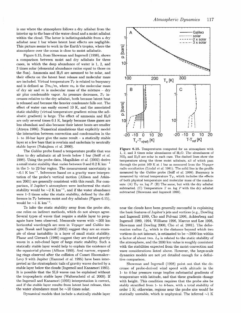
is one where the atmosphere follows a dry adiabat from the interior up to the base of the water cloud and a moist adiabat within the cloud. The latter is indistinguishable from a dry adiabat near 1 bar where latent heat effects are negligible. This picture seems to work in the Earth's tropics, where the atmosphere over the ocean is close to moist adiabatic.

Figure 6.15, from Showman and Ingersoll (1998), shows a comparison between moist and dry adiabats for three cases, in which the deep abundance of water is 1, 2, and 3 times solar (elemental abundance ratios equal to those on the Sun). Ammonia and H2S are assumed to be solar, and their effects on the latent heat release and molecular mass are included. Virtual temperature Tv is related to buoyancy and is defined as Tmo/m, where mo is the molecular mass of dry air and m is molecular mass of the mixture - dry air plus condensable vapor. As pressure decreases, Tv in­creases relative to the dry adiabat, both because latent heat is released and because the heavier condensate falls out. The effect of water can easily exceed 10 K, and the associated static stability (virtual temperature gradient minus the adi­abatic gradient) is large. The effect of ammonia and H2S are only several times 0.1 K, largely because these gases are less abundant and also because their latent heats are smaller (Atreya 1986). Numerical simulations that explicitly model the interaction between convection and condensation in the 1- to 10-bar layer give the same result - a statically stable layer at a few bars that is overlain and underlain by neutrally stable layers (Nakajima et al. 2000).

The Galileo probe found a temperature profile that was close to dry adiabatic at all levels below 1 bar (Seiff et al. 1998). Using the probe data, Magalhaes et al. (2002) derive a small static stability that varies between 0 and 0.2 K km - 1

in the 1- to 22-bar region. The measurement uncertainty is rv0.1 K km- 1

. Inferences based on a gravity wave interpre­tation of the probe's vertical motion (Allison and Atkin­son 2001) are generally consistent with this result. For com­parison, if Jupiter's atmosphere were isothermal the static stability would be rv2 K km- 1

, and if the water abundance were 1-3 times solar the static stability, defined by the dif­ference in Tv between moist and dry adiabats (Figure 6.15), would be rv1 K km- 1

.

To infer the static stability away from the probe site, one relies on indirect methods, which do not always agree. Several types of waves that require a stable layer to prop­agate have been observed. Mesoscale waves with rv300 km horizontal wavelength are seen in Voyager and Galileo im­ages. Bosak and Ingersoll (2002) suggest they are an exam­ple of shear instability in a layer of small static stability. Flasar and Gierasch (1986) suggest they are ducted gravity waves in a sub-cloud layer of large static stability. Such a statically stable layer would help to explain the existence of the equatorial plumes (Allison 1990). And narrow, expand­ing rings observed after the collision of Comet Shoemaker­Levy 9 with Jupiter (Hammel et al. 1995) have been inter­preted as the stratospheric tails of gravity waves ducted by a stable layer below the clouds (Ingersoll and Kanamori 1995). It is possible that the SL9 waves can be explained without the tropospheric stable layer (Walterscheid et al. 2000). If the Ingersoll and Kanamori (1995) interpretation is correct, and if the stable layer results from latent heat release, then

the water abundance must be rvlO times solar. Dynamical models that include a statically stable layer

Atmospheric Dynamics 117

A 1

10

100 200

8 1

-20 -10 0 10 20 Tv-T v(ref) [K]

1

10

---Galileo ................. solar - - - - - -2 x solar -·-·-·-· 3 x solar

300

c l I I

I I

I I

l I

I I

,Jf .. , : I \

I 1

-20 -1 0 0 1 0 20 T-Tref [K]

Figure 6.15. Temperatures computed for an atmosphere with 1, 2, and 3 times solar abundances of H20. The abundances of NH3 and H2S are solar in each case. The dashed lines show the temperature along the three moist adiabats, all of which pass through the point 169 K at 1 bar as measured from the Voyager radio occultation (Lindal et al. 1981). The solid line is the profile measured by the Galileo probe (Seiff et al. 1998). Buoyancy is measured by virtual temperature Tv, which includes the effects of both physical temperature and molecular mass of the conden­sate. (A) Tv vs. log P. (B) The same, but with the dry adiabat subtracted. (C) Temperature T vs. log P with the dry adiabat subtracted (Showman and Ingersoll 1998).

near the clouds have been generally successful in explaining the basic features of Jupiter's jets and vortices (e.g., Dowling and Ingersoll 1989, Cho and Polvani 1996, Achterberg and Ingersoll 1989, 1994, Williams 1996, Marcus and Lee 1998, Showman and Dowling 2000, Cho et al. 2001). The defor­mation radius Ld, which is the distance beyond which two vortices do not interact, is estimated to be rv2000 km within a factor of about two. Ld is related to the static stability of the atmosphere, and the 2000 km value is roughly consistent with the stabilities expected from the moist-convection and wave considerations listed above. However, the large-scale dynamics models are not yet detailed enough for a defini­tive comparison.

Showman and Ingersoll (1998) point out that the de­crease of probe-derived wind speed with altitude in the 1- to 4-bar pressure range implies substantial gradients of temperature with latitude, and that these gradients change with height. This condition requires that the probe site be stably stratified from 1- to 4-bars, with a total stability of

order 1 K; otherwise, regions near the probe site would be statically unstable, which is unphysical. The inferred rv 1 K

118 Ingersoll et al.

stability between 1 and 4 bars at the probe site is consistent with the recent probe analyses of Magalhaes et al. (2002).

The static stability measured by the probe is less than that suggested by the pre- Galileo wave-duct and moist­convection arguments. Showman and Dowling (2000) and Frieclson and Orton (1999) point out, however, that hot spots are probably the troughs of a large-scale wave, in which columns of air have been forced clown and vertically stretched by a factor of several. This mechanism would de­crease the mean static stability and push the high static stability region associated with the water condensation level (which was originally near 7 bars, Figure 6.15) clown to pres­sures greater than 22 bars, deeper than observed by the probe (Showman and Ingersoll 1998). The low static sta­bilities measured by the probe are therefore perhaps not representative of Jupiter as a whole.

6.5 MOIST CONVECTION AND LIGHTNING

6.5.1 Lightning Distribution

Voyager, Galileo, and Cassini detected lightning in long­exposure images of Jupiter's nightsicle (Borucki and Mag­alhaes 1992, Little et al. 1999, Gierasch et al. 2000, Porco et al. 2003). The lightning strikes were concentrated in clus­ters, suggesting that several discrete storms produced multi­ple strikes during each of the exposures. Twenty-six unique storms were documented in the two Galileo data sets. The lo­cations of lightning clusters have been correlated with the lo­cations of small, bright clouds on claysicle images. Although data are scarce, these thunderstorm clusters appear to be associated with high levels of humidity (Roos-Serote et al. 2000) and clouds at deep levels where water would be ex­pected to condense (Banfield et al. 1998).

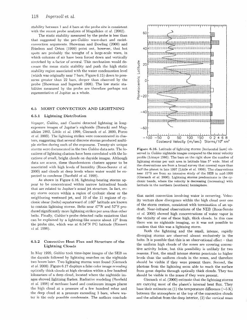
As shown in Figure 6.16, lightning-bearing storms ap­pear to be concentrated within narrow latitudinal bands that are related to Jupiter's zonal jet structure. In fact, ev­ery storm occurs within a region of cyclonic shear or the neighboring westward jet, and 10 of the 11 regions of cy­clonic shear (belts) equatorwarcl of ±60° latitude are known to contain lightning storms. Belts near 47°N and 52°8 pro­duced significantly more lightning strikes per area than other belts. Finally, Galileo's probe detected radio emissions that can be explained by a lightning-like source about 12° from the probe site, which was at 6.54°N PG latitude (Rinnert et al. 1998).

6.5.2 Convective Heat Flux and Structure of the Lightning Clouds

In May 1999, Galileo took time-lapse images of the SEB on the clayside followed by lightning searches on the nightside two hours later. Two lightning storms were found (Gierasch et al. 2000). Figure 6.17 displays a false color image revealing optically thick clouds at high elevation within a few hundred kilometers of a deep cloud, located where the nightside im­ages showed lightning flashes. Radiative modeling (Banfield et al. 1998) of methane band and continuum images places the high cloud at a pressure of a few hundred mbar and the deep cloud at a pressure exceeding 3 bars, where wa­ter is the only possible condensate. The authors conclude

··-60

·-· 1 00 --50 0 50 1 00 1 50 0 2 4 6 8 Eastward Velocity {rn/sec) Storms/1 09 krn2

Figure 6.16. Latitude of lightning storms (horizontal lines) ob­served in Galileo nightside images compared to the zonal velocity profile (Limaye 1986). The bars on the right show the number of lightning storms per unit area in latitude bins 5° wide. Most of the observations are from a broad survey that covered more than half the planet in late 1997 (Little et al. 1999). The observations near 15°S are from an intensive study of the SEB in mid-1999 (Gierasch et al. 2000). Lightning storms predominate in the cy­clonic bands, where the velocity is decreasing (increasing) with latitude in the northern (southern) hemisphere.

that moist convection involving water is occurring. Veloc­ity vectors show divergence within the high cloud over one of the storm centers, consistent with termination of an up­draft. Near-infrared observations of the NEB (Roos-Serote et al. 2000) showed high concentrations of water vapor in the vicinity of one of these high, thick clouds. In this case there was no nightside imaging, so it was not possible to confirm that this was a lightning storm.

Both the lightning and the small, intense, rapidly diverging storms are observed almost exclusively in the belts. It is possible that this is an observational effect - that the uniform high clouds of the zones are covering convec­tive activity below, but this possibility is unlikely for two reasons. First, the small intense storms penetrate to higher levels than the uniform clouds in the zones, and therefore should be visible if they were present there. Second, the photons from the lightning seem able to reach the surface from great depths through optically thick clouds. They too should be visible in the zones if they were present.

Gierasch et al. (2000) estimate that the lightning storms are carrying most of the planet's internal heat flux. They base their estimate on (1) the temperature difference (rv5 K) between the atmosphere at the top of the convective clouds and the adiabat from the deep interior, (2) the vertical mass

.](}

-12

-14

-16

2&0 Tl5 270 265

Figure 6.17. Lightning storms (Gierasch et al. 2000) in the southern hemisphere. The top panel is a superposition of a continuum wavelength (756 nm) in the red plane, a medium methane band (727 nm) in the green plane, and a strong methane band (889 nm) in the blue plane. The location of lightning is shown by the blue overlay on to a continuum image in the middle panel. Note the close proximity of red (deep) features and bright white (high) features to the flash locations. The bottom panel shows velocity vectors derived from three time-steps in the continuum. The flags point downwind, and the largest flag corresponds to a speed of 70 m s·1• The large-scale flow structure is eastward near the top of the frame (the north edge) and westward near the bottom. In the southern hemisphere this represents cyclonic shear. Approximate latitude and longitude are indicated on the bottom panel. This region is -30° west of the Great Red Spot. At the time of going to press a colour version of this figure was available for download from http://www.cambridge.org/9780521035453.

transport, which they get from the rate of horizontal diver­gence, and (3) the number of convective storms per unit surface area. The latter estimate comes from earlier Galileo observations that surveyed most of the planet's surface for lightning (Little et al. 1999).

6.5.3 Energy of Lightning Flashes

The measurable quantities are optical energy per flash and average optical power per unit area. Flash rate and color are measurable in principle. The optical range is here defined by the transmission of the Gal ilea clear filter, which goes from 385 nm to 935 nm (Little et al. 1999). One assumes that the photons are emitted uniformly in all directions. This gives a lower bound on the energy because clouds above the

flash site may scatter the photons back down where they are absorbed.

Atmospheric Dynamics 119

Jovian lightning occurs in storms whose sizes range from 200 km to over 1000 km and whose separation distance is rv104 km (Little et al. 1999). A 1-min exposure captures 10-20 flashes, which therefore overlap in the image. Overlap is not a problem if one is calculating the average optical power of the storm, but it prevents one from estimating the prop­erties of individual flashes. Fortunately, the Galileo camera captured three lightning storms in a "scanned" frame - a 59.8 s exposure that was deliberately smeared across the disk so that each storm left a trail of bright dots where the individual flashes occurred. The brightest flash in the scanned frame was 1.6 x 1010 J (Little et al. 1999). This is three times brighter than the largest terrestrial superbolts (Borucki et al. 1982). Smaller flashes are more numerous, but most of the storms' optical energy is carried in the largest flashes. The detection threshold for the Galileo and VoyageT cameras is about 2 x 108 J, which is larger than the aver­age terrestrial flash. Thus it is not possible to compare the global flash rates (number of flashes per unit area per unit time). However the average optical power per unit area is about the same for Earth and Jupiter, 3-4 x 10-7 W m- 2

,

even though the convective heat fluxes differ by more than an order of magnitude (rv8Q W m- 2 for Earth vs. rv6 W m- 2 for Jupiter) and the hydrologic cycles are fundamen­tally different.

The spectral energy density (W nm -l) measured by Gal ilea was greatest in the red filter, next greatest in vio­let, and least in green. The Cassini Ho: filter (centered on a strong line of atomic hydrogen at 656 nm) had the highest spectral energy density of all. While these results are con­sistent with a mixture of line and continuum emission in a hydrogen-helium atmosphere (Borucki et al. 1996), it is dif­ficult to infer physical properties of the lightning (discharge rate, temperature, or pressure) from these data alone.

6.5.4 Depth of Lightning

Since the photons are diffusing up through the intervening clouds, the depth of the lightning is roughly proportional to the width of the bright spot in the image. Width is defined as the half-width at half-maximum (HWHM), the radius of the circle where the intensity is one-half the value at the center of the spot. Scattering models put the ratio depth/HWHM in the range 1-2 (Borucki and Williams 1986, Little et al. 1999, Dyudina et al. 2002). The difficulty is finding light­ning flashes that are well resolved (pixel size ::;25 km), not overlapped, and not saturated.

Borucki and Williams (1986) report that the average HWHM for lightning observed in the VoyageT images is 55 ± 15 km. The HWHMs for six Galileo flashes are 87, 69, 37, 72, 42, and 50 km (Little et al. 1999, Dyudina et al. 2002). This puts the average depth in the range 60-120 km, depending on the parameters of the scattering model. The largest flashes could be even deeper.

With these large depths the lightning could be below the freezing level or even below the base of the water cloud, unless the water abundance is much higher than implied by solar values of the 0 /H ratio. The radiative properties of the clouds introduce a large (factor of 2) uncertainty. Not only are the radiative properties uncertain, but the shape of the

clouds are uncertain and are apparently not plane-parallel. Optical depth is greatest over the lightning and falls off with

120 Ingersoll et al.

horizontal distance (Dyudina et al. 2002). There is a small possibility that some of the flashes are doubles. Nevertheless, the conclusion is that the lightning flashes are deep - that they must be occurring within or below the jovian water cloud (Little et al. 1999).

6.5.5 Models of Moist Convection

Conrath and Gierasch (1984) discussed the relative buoy­ancy effects of latent heat release, hydrogen ortho-para con­version, and molecular weight differentiation on the outer planets and found that all three are in principle capable of causing density perturbations on the order of 1%. Smith and Gierasch (1995) showed that ortho-para effects are less im­portant for Jupiter than they are for Uranus and Neptune. Detailed modeling of moist buoyancy effects on Jupiter, with the environment (in which the plume is imbedded) fixed by initial conditions, yielded updraft velocities as high as tens of m s- 1 (Stoker 1986, Lunine and Hunten 1987). Self­consistent convective adjustment experiments (Delgenio and McGrattan 1990) gave layered profiles in the vertical and a subsaturated, stably stratified mean state.

Convective adjustment predicts mean profiles but not detailed flow fields, which are necessary eventually to explain charge separation and lightning. Yair et al. (1995, 1998) use an axisymmetric numerical flow model to study examples of moist convection. Hueso and Sanchez-Lavega (2001) and Hueso et al. (2002) developed a three-dimensional numerical model of moist convective storms that include vertical wind shears. Again an environmental stratification and specific initial conditions are imposed. These authors obtain flows consistent with precipitation and lightning when sufficient water vapor is introduced (OIH 2:: solar) and low stability is assumed.

The fact that lightning storms and moist convection seem to occur in the cyclonic belts needs an explanation, particularly since the air in the belts is sinking, at least in the upper troposphere. On Earth moist convection is as­sociated with low-level convergence and rising motion. One possibility is that the air in the belts is rising in the lower tro­posphere, with horizontal divergence at intermediate levels (Ingersoll et al. 2000). Such divergent flow might be driven by the eddy flux pu'v', which accelerates the jets on either side of the belt. Balancing the eddy acceleration of an east­ward (westward) jet requires transport of low (high) an­gular momentum air from higher (lower) latitudes. Since the eastward jets are on the equatorward sides of the belts and the poleward sides of zones, the net result is horizontal divergence in the belts and horizontal convergence in the zones. The updraft in the lower troposphere beneath the belts brings water vapor up from the interior and leads to moist convection.

6.6 MODELS OF THE ZONAL JETS

6.6.1 Banding Controlled in the Weather Layer

Two length scales have been invoked to explain the widths of the zonal jets. The first is the deformation radius Ld = NH/1!1, where N is the Brunt-VaisaJa frequency (the buoy­ancy frequency), H is the pressure scale height (~vertical

scale of motion), and f = 2Dsin(<f) with n the planet's angular velocity and ¢> the latitude (e.g., Pedlosky 1987). Attributed to Rossby, Ld is the horizontal distance beyond which two vortices do not strongly interact. Alternatively, it is the maximum size of features for which the fluid is barotropic and vertical stretching of vortex tubes is negli­gible. The deformation radius is relevant where f =j:. 0, i.e., away from the equator. If there is a stable layer associated with moist convection within the water cloud (Achterberg and Ingersoll 1989, Ingersoll and Kanamori 1995), then Ld may be written cllfl where c is the speed of gravity waves that are ducted in the layer. Its value is estimated to be rv2000 km in Jupiter's troposphere at mid latitudes, with both the uncertainty and the natural variability probably a factor of 2 in each direction. The value of Ld could be much smaller if the low values of N measured by the Galileo probe are typical of the planet as a whole.

The second length scale is Lf3 = (Uif3) 112, where U

is the magnitude of the horizontal velocity, (3 = df I dy = 20 cos( <P) I a is the planetary vorticity gradient, and a is the planetary radius. Attributed to Rhines, it is the scale above which the speed of a barotropic Ross by wave is greater than the wind speed. Alternatively, it is the critical width of the zonal jets below which they might be unstable. The barotropic stability criterion says that the flow is stable pro­vided Qy = (3- ilyy > 0 at all latitudes, where the subscripts denote differentiation with respect to y. Here Qy is the ab­solute vorticity gradient, the sum of the planetary vorticity gradient (3 and the relative vorticity gradient -ilyy. Voyager data imply that fiyy varies between ±2(3 and therefore that the criterion is violated (Ingersoll et al. 1981, Limaye 1986). Reproducing this observation is a major challenge for the models. One possibility is that the variation of wind with altitude, which is ignored in barotropic models, is affecting the stability of the flow.

Rhines (1975) demonstrated that zonal jets emerge from decaying turbulence on a (3-plane- a planar coordinate sys­tem that preserves the important effects of the planet's cur­vature and rotation. Williams (1978) first applied these ideas to Jupiter. These ,8-turbulence models have sorne common features. First, they describe motion in a thin layer, either on a ,8-plane or on the surface of a sphere; motions in the planet's interior are neglected. Second, they rely on small­scale forcing. The classic inverse cascade models (Vallis and Maltrud 1993, Huang and Robinson 1998, Marcus et al. 2000, Sukoriansky et al. 2002) have positive and negative sources of vorticity at small scales. The baroclinic models (Panetta 1993) have an unstable temperature gradient that produces eddies at the Ld scale. Other models (Williams 1978, Cho and Polvani 1996) start with an initial eddy field that evolves without dissipation to a set of zonal jets. There is a strong anisotropy between the zonal and meridional di­rections; zonal jets develop in all the models. But in all cases the resulting jets have ilyy < (3; they are too wide and too weak to violate the barotropic stability criterion and there­fore do not fully agree with the Jupiter data.

Another mystery is why Jupiter has weaker winds than any other giant planet despite its greater radiative en­ergy fluxes - absorbed and emitted power per unit area. For example, Neptune's winds are rv3 times stronger than Jupiter's, but the radiative fluxes at Neptune are rv20 times weaker. One possibility (Ingersoll 1990, Ingersoll et al. 1995)

is that the radiative fluxes determine the level of atmo­spheric turbulence, which dissipates the energy of the large­scale winds. If the turbulence levels decrease by a large amount as the radiative fluxes decrease, and the energy sources that drive the winds decrease by a smaller amount, the large-scale winds would increase. By this token, the high­speed jets of Neptune are coasting in an atmosphere where dissipation is low. Jupiter's atmosphere is more turbulent, which limits the speed of the large-scale winds. Interestingly, Earth has the weakest large-scale winds and the strongest radiative heating of any atmosphere-covered planet in the solar system.

6.6.2 Deep Winds and Stability of the Jets

Jupiter's strong, narrow jets are unstable if one assumes that the winds are confined to a thin horizontal layer. For instance, Dowling and Ingersoll (1989) showed that Jupiter's cloud-top winds suffer barotropic instability and evolve away from what is observed when initialized in a shallow-water model with no deep circulation. However, Ingersoll and Cuong (1981) found that the upper-layer wind profile is sta­ble if it rests hydrostatically on a co-moving deep lower layer whose density is greater than that of the upper layer. This is an extension of the idea that the observed zonal jets are the surface manifestation of differentially rotating cylinders con­centric with the planet's rotation axis (Busse 1976). Ingersoll and Pollard (1982) showed that the rotating cylinders could be stable even though they violate the barotropic stability criterion because that criterion applies only to motions in thin shells. They developed a criterion that applies to mo­tions inside a compressible fluid sphere, where the effective {3 is negative and is 2 or 3 times larger than the traditional {3. Jupiter's observed winds are closer to marginal stability according to this criterion. However, the rotating cylinders penetrate into the interior where the electrical conductivity is high and the magnetic field may interfere with the flow (Kirk and Stevenson 1987). A complete theory would take these hydromagnetic effects into account.

Orsolini and Leovy (1993a, 1993b) examined the linear instability problem in cases where there is a deep circulation, to see whether the motions in the overlying atmosphere can be stabilized. They found that jets that decay with height are more stable that those that do not. This agrees with work by Pirraglia (1989) and is consistent with the jet decay with height inferred for Jupiter via the thermal-wind analysis. These two studies demonstrate the potential importance of the deep flow for the stability of the jets, but they do not discuss how the deep flow is maintained.

Dowling and Ingersoll (1988, 1989) deduced the nature of the deep circulation by observing changes in absolute vor­ticity as parcels move around the GRS and white oval BC. Changes in absolute vorticity are due to vortex tube stretch­ing, which arises when the parcels cross the pressure ridges associated with the flow underneath. The analysis produced a family of possible deep circulations with La as the un­known scaling factor. For each case, the deep flow is not in solid rotation; it seems to have a jet-like structure some­what like that observed in the upper layer. Dowling (1993) showed that this family of abyssal circulations corresponds

to the special case Ld = Lf3, where (3 is the full gradient of potential vorticity including the vertical stretching term.

Atmospheric Dynamics 121

This condition corresponds to the case of marginal stability with respect to a criterion that traces back to Kelvin and is now known as Arnol'd's second stability criterion (although it is notably absent from most meteorology textbooks). It al­lows a shear flow to be stable even though the flow does not satisfy other, better-known stability conditions. Here again, the abyssal circulation plays an essential role in stabilizing the flow in the upper layers.

By assuming that the rv450 m s- 1 speed (Hammel et al. 1995) of the dark ring seen propagating outward from each of the Comet Shoemaker-Levy 9 impact sites is the grav­ity wave speed in Jupiter's atmosphere (not a firmly estab­lished fact), Dowling (1995b) singled out the corresponding member in the family of deep circulations mentioned above to predict that Jupiter's westward jets change little with depth, but that its eastward jets increase in strength by 50-100% with depth. This prediction for the eastward jets closely matches the subsequent results of the Galileo probe Doppler wind experiment, with the caveat that the probe's latitude of 7°N is too close to the equator for the strong Cori­olis effect assumed by this quasigeostrophic (mid-latitude) theory.

6.6.3 Banding Controlled in the Interior

Several groups have considered the possibility that Jupiter's jet streams are rooted deep in the interior where the planet's internal heat source drives convection, and where there is no confinement of motions inside a thin spherical shell. Busse (1976) investigated such convection, and showed that it can generate alternating jets at the top of the convecting sphere. Condie and Rhines (1994) studied a laboratory analog con­sisting of a rotating bowl of warm water that is uniformly cooled at the free surface. The cooling generates convec­tion cells that give rise to azimuthal jets when they en­counter the free surface. Manneville and Olson (1996) find symmetric bands and zonal jets in a rotating convecting fluid sphere. Sun et al. (1993) carried out numerical sim­ulations of a rapidly rotating, deep fluid shell and achieved a broad eastward flow at the equator with alternating jets at higher latitudes. However, the amplitude of their zonal flow is an order of magnitude less than the amplitude of the non-axisymmetric flow; in other words, the jets are barely discernable through the large noise of the convection. Zhang and Schubert (2000) developed a model that combines con­vection in the deep interior with an overlying stable atmo­sphere. They find that strong motions can concentrate in the atmosphere as a result of convection that is driven ther­mally in the deep interior, a phenomenon they term "tele­convection." More coupled atmosphere-interior models like this one are needed. Eventually the atmospheric component should include effects of moist convection, and the interior component should include the effects of electrical conduc­tivity and magnetic fields.

6.6.4 Modes of Internal Heat Transfer

Ingersoll and Porco (1978) pointed out that if Jupiter has a convective interior, only very small lateral temperature gra­dients should be expected at the outer edge of the convective

region. If the emission to space is from the top of the con­vective interior, it should be uniform with latitude. This is

122 Ingersoll et al.

the accepted explanation for the observation (Figure 6.12) that emission to space on Jupiter is essentially independent of latitude (Ingersoll et al. 1976, Pirraglia 1984). But nei­ther the zonal mean insolation nor the emission to space is determined very accurately by observations, and dynam­ically important temperature gradients at, say, the 10-bar level cannot be ruled out. Temperature contrasts of only a few degrees would be important for the dynamics, and could possibly explain the mean eastward bias in globally averaged surface wind (Gierasch 1999).

A new wrinkle was introduced when Guillot et al. (1994) pointed out that a radiative zone might exist in Jupiter (and Saturn) near the depth where the temperature reaches about 2000 K. This occurs where the pressure is a few tens of kilobars and the depth is a few percent of the radius. At this temperature the peak of the Planck function has shifted to near 5 J.1m, where jovian material has relatively low opacity. Since 1994, Guillot has discovered new sources of opacity, and this radiative zone may not exist on Jupiter. If it does exist, the Ingersoll and Porco reasoning should be reexamined. Gierasch (1999) experimented with radiative­convective models that include a radiative zone and no lat­eral heat transport. These models show that even a modest radiative zone would break the tight constraint on latitudi­nal temperature gradients that is imposed by a fully convec­tive interior.

A major question about the outer planets is the depth of the dynamical region that produces the visible jets and spots. Without a solid surface and without a stability tran­sition there is no externally imposed boundary to form a base, leading to debate about "deep cylinder" flow configura­tions that extend through the planet as opposed to "shallow weather layer" configurations (Busse 1976, Allison 2000). If a radiative zone exists, it could be the location of the "windy jovian thermocline" discussed by Allison (2000). Allison's thermocline is a stable layer that is conjectured to close off the weather layer circulation and separate it from the deep interior. In general, the basic state stratification is a fun­damental parameter affecting dynamics and heat transport and it is of high priority to determine whether a radiative zone exists on Jupiter and Saturn.

6.6.5 Banding Controlled by Tides

The third class of hypotheses concerning the control of Jupiter's jet streams involves the intriguing possibility that the winds are shaped and accelerated by satellite tides. Ioan­nou and Lindzen (1994) showed that if the interior of Jupiter is even modestly stable to convection, tides that are domi­nated by higher-order Hough modes can couple to it. These tend to produce banding with alternating accelerations on the order of 1 em s- 1d- 1

, which is significant. The authors find that the dominant tides come from Io, Titan, Ariel, and Triton, respectfully, for Jupiter, Saturn, Uranus, and Neptune. This idea adds to the motivation to search for ob­servational evidence of the tidal response at Jupiter's cloud level.

6.6.6 Equatorial Superrotation

Jupiter, Saturn, Venus, and the Sun exhibit equatorial su­perrotation -the atmosphere rotates faster near the equator

than at other latitudes. Earth, Uranus, and Neptune exhibit equatorial subrotation. Although the equator of Jupiter is a local minimum of zonal velocity due to the zonal jet max­ima at ±7° PG latitude (Figure 6.2), it is a local maximum of absolute angular momentum. Since rings of fluid circling the planet at constant latitude tend to conserve their an­gular momentum as they move, any mixing between rings will reduce the angular momentum at the equator. A the­orem due to Hide (1970) states that a circulation that is symmetric about the axis of rotation (one with no eddies) cannot sustain a local maximum of angular momentum. The inference is that the equatorial maximum on Jupiter is main­tained by eddy fluxes, e.g., pressure variations in longitude. In a paper on the superrotation of Venus, Gierasch (1975) noted that friction tends to mix angular momentum down the gradient of angular velocity, toward a state of solid body rotation. For Jupiter, this down-gradient mixing is toward the equator, at least up to the latitude of the zonal jets at ±7°. Since friction in a planetary atmosphere involves turbulent eddies, the conclusion is that Jupiter's equatorial superrotation is maintained by eddy fluxes. Whether the mixing is from higher latitudes or from lower altitudes is unknown.

Most inverse-cascade models (Section 6.6.1) use a {3-plane geometry, and so are unable to address the question of equatorial superrotation. Cho and Polvani (1996) consider decaying barotropic turbulence in a thin layer on a full ro­tating sphere. Zonal jets develop at mid latitudes, but the equator subrotates as on Uranus and Neptune. Yano et al. (2002) consider decaying barotropic turbulence in a deep fluid sphere, where the {3 effect has the opposite sign from that in a shallow surface layer (Ingersoll and Pollard 1982). In this case a superrotating flow develops at the equator as on Jupiter and Saturn. This is a suggestive result, but it is not a proof that the fluid sphere model is correct, since Venus superrotates and Earth does not, and both atmospheres are thin compared to the radius of the planet.

6.7 MODELS OF DISCRETE FEATURES

6. 7.1 Stable Vortices

The simplest model that produces stable vortices is an invis­cid, two-dimensional, non-divergent flow with shear (Moore and Saffman 1971, Kida 1981). The fluid has uniform vor­ticity inside an isolated patch and a different uniform vor­ticity outside. A steady, stable configuration occurs when the anomalous patch has elliptical shape, with the long axis oriented parallel to the flow at infinity (east-west on the giant planets). The aspect ratio (ratio of long axis to short axis) depends on the ratio of the vorticity inside to that out­side the patch. Finite amplitude perturbations lead to stable oscillations in the aspect ratio and orientation.

Polvani et al. (1990) showed that this "Kida vortex" model does a good job of matching the observations of vor­tices on the giant planets. For the GRS and white ovals of Jupiter, where we have measurements of the vorticity inside and outside, the model accurately accounts for the average aspect ratio (Ingersoll et al. 1995). For the Great Dark Spot (GDS) of Neptune, which oscillates in aspect ratio and orien­tation, the model accurately accounts for the relative phase

and relative amplitude of the two oscillations. The model does not explain the amplitude itself, which is a free pa­rameter of the theory, nor does it account for the observed shedding of filaments.

It is remarkable that the Kida vortex model works as well as it does. It has no vertical structure, no gradient in the ambient vorticity ((3 effect), no forcing, and no dissipation. Introducing these effects adds to the complexity of the mod­els and greatly increases the number of free parameters. In fact, stable vortices exist in models with a wide variety of as­sumptions about the vertical thermal structure, the flow un­derneath, and the energy source (Ingersoll and Cuong 1981, Williams and Yamagata 1984, Marcus 1988, Williams and Wilson 1988, Dowling and Ingersoll 1989, Williams 1996, 2002, LeBeau and Dowling 1998, Marcus et al. 2000, Cho et al. 2001, Youssef and Marcus 2003). Stable vortices form also in laboratory experiments (Nezlin 1986, Read 1986).

The GRS oscillates in longitude with rv1 ° amplitude (peak-to-peak) and 90-day period (Solberg 1969, Trigo­Rodriguez et al. 2000). Other jovian spots oscillate in longi­tude as well (Peek 1958). Neptune's second dark spot discov­ered in Voyager 2 images oscillated in longitude with ±45° amplitude and 36-day period (Ingersoll et al. 1995). The Kida model has oscillations in orientation and aspect ratio only. Achterberg and Ingersoll (1994) developed a model in which the longitude oscillations arise when the top and bot­tom halves of the vortex orbit around a common vertical axis. They obtained peak-to-peak amplitudes up to 15°, but they were not able to reproduce the large-amplitude oscil­lation of the Neptune spot because the two halves of the vortex tended to separate and drift off separately.

These inviscid theories shed no light on what maintains the vortices or their oscillations against dissipation. Obser­vations of mergers suggest that the large vortices feed on the smaller ones. The inverse cascade of energy from small scales to large scales apparently maintains the vortices as well as the zonal jets. One then must ask where do the small vor­tices get their energy? The possibilities include: instability associated with latitudinal temperature gradients and the corresponding vertical shear, horizontal shear instability of the zonal jets, and moist convection. Finding the answer is an active area of current research.

6. 7.2 Statistical Mechanics Models

An entirely different approach, one that bypasses the tem­poral development of the flow, is to solve for the equilib­rium state that maximizes a global integral that is analo­gous to the entropy in statistical mechanics (Sommeria et al. 1991, Miller et al. 1992, Michel and Robert 1994, Steg­ner and Zeitlin 1996, Turkington et al. 2001, Bouchet and Sommeria 2002). The parcels are allowed to mix as if they were chemically distinct molecules, such that each parcel conserves its initial value of potential vorticity (PV). This conservative mixing is appropriate for an inviscid, adiabatic fluid, but it is not clear how it would work in a real at­mosphere, where the PV values may change during mixing. Also, the initial PV distribution is arbitrary and is not deriv­able from the maximum-entropy principle. The proponents

of this approach point out that the equilibrium states agree with numerical simulation (e.g., Marcus 1988) and with the

Atmospheric Dynamics 123

steady shapes of jovian vortices. The model does not account for the oscillations, since the equilibrium state is steady.

Turkington et al. (2001) propose using the equilibrium statistical theory for inverse modeling of the small-scale vor­ticity distribution. They start with realistic zonal jets and the underlying zonal flow as defined by Dowling (1995b ). The theory gives one GRS, one white oval, and realistic zonal jets - but only if the initial vorticity distribution is skewed toward anticyclonic values. Turkington et al. cite the recent Galileo results (Gierasch et al. 2000, Ingersoll et al. 2000) that support the occurrence of intense small-scale anticy­clonic forcing.

6.7.3 Equatorial Hot Spots and the Galileo Probe

In 1995, the Galileo probe took in situ measurements of composition, winds, temperature, and clouds from about 0.4 bars to 22 bars, a 150-km range of altitude. These mea­surements have raised questions about conditions below the clouds. Before the probe's entry, many experts thought that the atmosphere would be well mixed below the condensation levels. That is, the ammonia mixing ratio would level off be­low 0. 7 bars, and the H2S and water mixing ratios would level off below 2 bars and 6 bars, respectively. Instead the ammonia mixing ratio leveled off at 10 bars, H2S leveled off at 16 bars, and water was still increasing with depth at 20 bars (Niemann et al. 1998, Folkner et al. 1998, Mahaffy et al. 2000). These observations require a dynamical explanation.

The probe entered one of Jupiter's 5-!-lm hot spots, where a hole in the visible cloud 5000 km wide allows 5-~-Lm radiation to escape. To explain the hole in the clouds and the depressed volatile abundances, several authors sug­gested that hot spots contain downdrafts that advect dry air from the upper troposphere down to rv20 bars or deeper. The simplest version of this idea has dense air that descends because it is convectively unstable (Atreya et al. 1999, Show­man and Ingersoll 1998, Baker and Schubert 1998). A diffi­culty is that any static stability from 1-10 bars (as seems to exist; see Section 6.4.4) would act to halt the descent. More­over, downdrafts produced in numerical simulations (Baker and Schubert 1998) are two orders of magnitude too small. The convective downdraft hypothesis also has problems with the wind shear, which tends to pull the hot spot apart in 1 or 2 days, and does not explain the layered distribution of volatiles.

The second idea hypothesizes that hot spots are the downwelling branch of an equatorially trapped wave (Fried­son and Orton 1999, Showman and Dowling 2000). Allison (1990) and Ortiz et al. (1998) documented wavelike behavior for the plumes and hot spots, and Showman and Dowling (2000) performed numerical simulations that support this idea. Air parcels that enter the hot spot from the west (at tens of m s- 1

) are deflected downward; the parcels return to their original altitudes a few days later as they exit the hot spot to the east. This downwelling wave model explains the layered structure in the ammonia, H2S, and water. Show­man and Dowling's (2000) simulations also suggest that the increase in winds with depth observed by the Galileo probe results from local dynamics at the south edge of hot spots and may not be a large-scale property of Jupiter's equato-

rial atmosphere. Although some issues remain, the model successfully explains the observed dryness as a local me-

124 Ingersoll et al.

teorological effect, and it is consistent with the idea that Jupiter's deep water abundance is at least solar.

6.8 UNANSWERED QUESTIONS AND POSSIBLE SOLUTIONS

Some of the big questions are: Why are the giant planets banded? What controls the speed and width of the zonal jets? Why are the jets stable? Where do the jets get their energy? Do the winds extend into the fluid interior? Why are the large vortices so stable? What are the clouds made of, and why are they colored? What is the composition of the deep atmosphere? What is the water abundance? How important is moist convection? Where does lightning occur, and what is its relation to global features? Many of these questions concern the deep atmosphere - its composition, thermal structure, and dynamics. Here we describe how ob­servations and modeling can provide the answers.

Gravity measurements can determine whether the deep atmosphere, 1000s of km down, is in solid-body rotation or has jet streams comparable in speed to the surface jets. The centrifugal forces associated with the deep jets cause a re-arrangement of mass that reveals itself in the planet's external gravity field. To sample the higher harmonics of the gravity field, it is best to have a polar orbiter or flyby with a low perijove.

Water is crucial to the meteorology of Jupiter and to the planet's history, since water ice is thought to have played a crucial role in the distribution of volatiles throughout the so­lar system (see Chapter 2). Both water and ammonia absorb in the microwave region and reveal themselves in the ther­mal emission coming from the planet at these wavelengths. A microwave radiometer on a spacecraft passing close to the planet could detect this radiation and measure the water and ammonia abundance at depths ranging from 1 bar to lOOs of bars.

Probes can measure gaseous abundances, including wa­ter, and can also measure temperature, cloud amount, scat­tered sunlight, and winds. The vertical temperature profile determines the dynamical coupling between the deep atmo­sphere and the surface layers. Stable stratification means they are uncoupled; neutral or unstable means they are cou­pled. Sunlight provides energy for the winds, which can be measured by Doppler tracking as the probe descends. A ma­jor lesson of the Galileo probe mission is that it is important to have multiple probes that enter Jupiter's atmosphere at different latitudes. It is also important that they return data to rv 100 bars. Both of these goals are within reach.

Progress will come as well from data already in hand and from theoretical modeling. Most of the Cassini data were not analyzed at the time of this writing; they could contain data on chemical tracers, temperatures, winds, wa­ter, ammonia, and lightning that answer some fundamen­tal questions. For instance, Galileo provided a snapshot of the lightning storms, but Cassini may allow us to track the storms over time, measure their motion, and determine their lifetimes. Since the lightning is generated at or below the base of the water cloud, the storms' motion could reveal in­formation about winds at depths that cannot be observed in dayside images.

Numerical models are a key tool for studying atmo-

spheres, and Jupiter's atmosphere is no exception. The data provide constraints on the models. Models of key processes like moist convection in a bottomless atmosphere need to be developed. The GCMs for Jupiter are less well constrained than GCMs for Earth or Mars, but that makes them all the more interesting. Meteorologists and oceanographers recog­nize Jupiter's value as a fluid dynamics laboratory. The goal is to capture the truth in a small range of parameter space. When the combined constraints of observation and theory rule out most of the hypotheses and the models all resem­ble each other, then we can truly claim to understand the dynamics of Jupiter's atmosphere.

Acknowledgements. We thank the many agencies that have funded planetary science research, and we thank the many people who have contributed to our knowledge of Jupiter's atmosphere.

REFERENCES

Achterberg, R. K. and A. P. Ingersoll, A normal-mode approach to jovian atmospheric dynamics, J. Atmos. Sci. 46, 2448-2462, 1989.

Achterberg, R. K. and A. P. Ingersoll, Numerical simulation of baroclinic jovian vortices, J. Atmos. Sci. 51, 541-562, 1994.

Allison, M., Planetary waves in Jupiter's equatorial atmosphere, Icarus 83, 282-307, 1990.

Allison, M., A similarity model for the windy jovian thermocline, Planet. Space Sci. 48, 753-774, 2000.

Allison, M. and D. H. Atkinson, Galileo probe Doppler residuals as the wave-dynamical signature of weakly stable downward­increasing stratification in Jupiter's deep wind layer, Geo­phys. Res. Lett. 28, 2747-2750, 2001.

Atkinson, D. H., J. B. Pollack, and A. Seiff, The Galileo probe Doppler wind experiment: Measurement of the deep zonal winds on Jupiter, J. Geophys. Res. 103, 22 911-22 928, 1998.

Atreya, S. K., Atmospheres and Ionospheres of the Outer Planets and their Satellites, Springer-Verlag, 1986.

Atreya, S. K., M. H. Wong, T. C. Owen, P. R. Mahaffy, H. B. Niemann, I. de Pater, P. Drossart, and T. Encrenaz, A com­parison of the atmospheres of Jupiter and Saturn: Deep at­mospheric composition, cloud structure, vertical mixing, and origin, Planet. Space Sci. 47, 1243-1262, 1999.

Baker, R. D. and G. Schubert, Deep convective entrainment by downdrafts in Jupiter's atmosphere, Icarus 136, 340-343, 1998.

Banfield, D., P. J. Gierasch, M. Bell, E. Ustinov, A. P. Ingersoll, A. R. Vasavada, R. A. West, and M. J. S. Belton, Jupiter's cloud structure from Galileo imaging data, Icarus 135, 230-250, 1998.

Barcilon, A. and P. J. Gierasch, A moist, Hadley cell model for Jupiter's cloud bands, J. Atmos. Sci. 27, 550-560, 1970.

Beebe, R. F. and T. A. Hockey, A comparison of red spots in the atmosphere of Jupiter, Icarus 67, 96-105, 1986.

Beebe, R. F. and L.A. Youngblood, Pre- Voyager velocities, accel­erations and shrinkage rates of jovian cloud features, Nature 280, 771-772, 1979.

Beebe, R. F., A. P. Ingersoll, G. E. Hunt, J. L. Mitchell, and J.-P. Muller, Measurements of wind vectors, eddy momentum transports, and energy conversions in Jupiter's atmosphere from Voyager 1 images, Geophys. Res. Lett. 7, 1-4, 1980.

Beebe, R. F., G. S. Orton, and R. A. West, Time-variable na­ture of the Jovian cloud properties and thermal structure: An observational perspective, in Time- Variable Phenomena in

the Jovian System, M.J.S. Belton, R.A. West, J. Rahe (eds), NASA, pp. 245-288, 1989.

Beebe, R. F., A. A. Simon, and L. F. Huber, Comparison of Galileo probe and Earth-based translation rates of Jupiter's equatorial clouds, Science 272, 841, 1996.

Borucki, W. J. and J. A. Magalhaes, Analysis of Voyager 2 images of jovian lightning, Icarus 96, 1-14, 1992.

Borucki, W. J. and M.A. Williams, Lightning in the jovian water cloud, J. Geophys. Res. 91, 9893-9903, 1986.

Borucki, W. J., A. Bar-Nun, F. L. Scarf, A. F. Cook, and G. E. Hunt, Lightning activity on Jupiter, Icarus 52, 492-502, 1982.

Borucki, W. J., C. P. McKay, D. Jebens, H. S. Lakkaraju, and C. T. Vanajakshi, Spectral irradiance measurements of sim­ulated lightning in planetary atmospheres, Icarus 123, 336-344, 1996.

Bosak, T. and A. P. Ingersoll, Shear instabilities as a probe of Jupiter's atmosphere, Icarus 158, 401-409, 2002.

Bouchet, F. and J. Sommeria, Emergence of intense jets and Jupiter's Great Red Spot as maximum-entropy structures, J. Fluid Mech. 464, 165-207, 2002.

Busse, F. H., A simple model of convection in the jovian atmo­sphere, Icarus 29, 255-260, 1976.

Cho, J. Y.-K. and L. M. Polvani, The morphogenesis of bands and zonal winds in the atmospheres on the giant outer planets, Science 273, 335-337, 1996.

Cho, J. Y.-K., M. de La Torre Juarez, A. P. Ingersoll, and D. G. Dritschel, A high-resolution, three-dimensional model of Jupiter's Great Red Spot, J. Geophys. Res. 106, 5099-5105, 2001.

Condie, S. A. and P. B. Rhines, Topographic Hadley cells, J. Fluid M ech. 280, 349-368, 1994.

Conrath, B. J. and P. J. Gierasch, Global variation of the para hydrogen fraction in Jupiter's atmosphere and implications for dynamics on the outer planets, Icarus 57, 184-204, 1984.

Conrath, B. J. and P. J. Gierasch, Retrieval of ammonia abun­dances and cloud opacities on Jupiter from Voyager IRIS spectra, Icarus 67, 444-455, 1986.

Conrath, B. J., F. M. Flasar, J. A. Pirraglia, P. J. Gierasch, and G. E. Hunt, Thermal structure and dynamics of the jovian atmosphere: 2. Visible cloud features, J. Geophys. Res. 86, 8769-8775, 1981.

Conrath, B. J., P. J. Gierasch, and S. S. Leroy, Temperature and circulation in the stratosphere of the outer planets, Icarus 83, 255-281, 1990.

Delgenio, A. D. and K. B. McGrattan, Moist convection and the vertical structure and water abundance of Jupiter's at­mosphere, Icarus 84, 29-53, 1990.

Deming, D., M. J. Mumma, F. Espenak, D. E. Jennings, T. Kostiuk, G. Wiedemann, R. Loewenstein, and J. Piscitelli, A search for P-mode oscillations of Jupiter: Serendipitous ob­servations of nonacoustic thermal wave structure, ApJ 343, 456-467, 1989.

Deming, D., D. Reuter, D. Jennings, G. Bjoraker, G. McCabe, K. Fast, and G. Wiedemann, Observations and analysis of longitudinal thermal waves on Jupiter, Icarus 126, 301-312, 1997.

Dowling, T. E., A relationship between potential vorticity and zonal wind on Jupiter, J. Atmos. Sci. 50, 14-22, 1993.

Dowling, T. E., Dynamics of jovian atmospheres, Annual Review of Fluid Mechanics 27, 293-334, 1995a.

Dowling, T. E., Estimate of Jupiter's deep zonal-wind profile from Shoemaker-Levy 9 data and Arnol'd's second stability crite­rion, Icarus 117, 439-442, 1995b.

Dowling, T. E. and A. P. Ingersoll, Potential vorticity and layer thickness variations in the flow around Jupiter's Great Red

Spot and white oval BC, J. Atmos. Sci. 45, 1380-1396, 1988. Dowling, T. E. and A. P. Ingersoll, Jupiter's Great Red spot as a

Atmospheric Dynamics 125

shallow water system, J. Atmos. Sci. 46, 3256-3278, 1989. Dyudina, U. A., A. P. Ingersoll, A. R. Vasavada, S. P. Ewald,

and the Galileo SSI Team, Monte Carlo radiative transfer modeling of lightning observed in Galileo images of Jupiter, Icarus 160, 336-349, 2002.

Fisher, B. M., High Time Resolution Infrared Imaging Observa­tions of Jupiter, Ph.D. thesis, University of California, San Diego, 1994.

Fisher, B. M., G. S. Orton, and C. Hasenkopf, Jovian longitudinal thermal structure in mid 1999, BAAS 33, 1045, 2001.

Flasar, F. M., Temporal behavior of Jupiter's meteorology, in Time- Variable Phenomena in the Jovian System, M. J. S. Belton, R. A. West, J. Rahe (eds), NASA, pp. 324-343, 1989.

Flasar, F. M. and P. J. Gierasch, Mesoscale waves as a probe of Jupiter's deep atmosphere, J. Atmos. Sci. 43, 2683-2707, 1986.

Flasar, F. M., B. J. Conrath, J. Pirraglia, P. C. Clark, R. G. French, and P. J. Gierasch, Thermal structure and dynamics of the jovian atmosphere: 1. The Great Red Spot, J. Geo­phys. Res. 86, 8759-8767, 1981.

Folkner, W. M., R. Woo, and S. Nandi, Ammonia abundance in Jupiter's atmosphere derived from the attenuation of the Galileo probe's radio signal, J. Geophys. Res. 103, 22 847-22 855, 1998.

Friedson, A. J., New observations and modelling of a QBO-like oscillation in Jupiter's stratosphere, Icarus 137, 34-55, 1999.

Friedson, A. J. and G. S. Orton, A dynamical model of Jupiter's 5-micron hot spots, BAAS 31, 1155, 1999.

Garcia-Melendo, E. and A. Sanchez-Lavega, A study of the stabil­ity of jovian zonal winds from HST images: 1995-2000, Icarus 152, 316-330, 2001.

Garcfa-Melendo, E., A. Sanchez-Lavega, J. M. Gomez, J. Lecacheux, F. Colas, I. Miyazaki, and D. Parker, Long­lived vortices and profile changes in the 23.7°N high-speed jovian jet, Icarus 146, 514-524, 2000.

Gehrels, T., Jupiter, University of Arizona Press, 1976. Gierasch, P. J., Meridional circulation and the maintenance of the

Venus atmospheric rotation, J. Atmos. Sci. 32, 1038-1044, 1975.

Gierasch, P. J., Radiative-convective latitudinal gradients for Jupiter and Saturn models with a radiative zone, Icarus 142, 148-154, 1999.

Gierasch, P. J. and B. J. Conrath, Dynamics of the atmospheres of the outer planets: Post- Voyager measurement objectives, J. Geophys. Res. 98, 5459-5469, 1993.

Gierasch, P. J., B. J. Conrath, and J. A. Magalhaes, Zonal mean properties of Jupiter's upper troposphere from Voyager in­frared observations, Icarus 67, 456-483, 1986.

Gierasch, P. J., A. P. Ingersoll, D. Banfield, S. P. Ewald, P. Helfen­stein, A. Simon-Miller, A. Vasavada, H. H. Breneman, D. A. Senske, and the Galileo Imaging Team, Observation of moist convection in Jupiter's atmosphere, Nature 403, 628-630, 2000.

Guillot, T., G. Chabrier, P. Morel, and D. Gautier, Nonadiabatic models of Jupiter and Saturn, Icarus 112, 354-367, 1994.

Hammel, H. B., R. F. Beebe, A. P. Ingersoll, G. S. Orton, J. R. Mills, A. A. Simon, P. Chodas, J. T. Clarke, E. DeJong, T. E. Dowling, J. Harrington, L. F. Huber, E. Karkoschka, C. M. Santori, A. Toigo, D. Yeomans, and R. A. West, HST imaging of atmospheric phenomena created by the impact of Comet Shoemaker-Levy 9, Science 267, 1288-1296, 1995.

Harrington, J., T. E. Dowling, and R. L. Baron, Jupiter's tro­pospheric thermal emission: 2. Power spectrum analysis and wave search, Icarus 124, 32-44, 1996.

Hatzes, A., D. D. Wenkert, A. P. Ingersoll, and G. E. Daniel­son, Oscillations and velocity structure of a long-lived cyclonic spot, J. Geophys. Res. 86, 8745-8749, 1981.

Hess, S. L. and H. A. Panofsky, The atmospheres of the other

126 Ingersoll et al.

planets, in Compendium of Meteorology, T. F. Malone (ed.), American Meteorological Society, pp. 391-400, 1951.

Hide, R., Equatorial jets in planetary atmospheres, Nature 225, 254, 1970.

Huang, H. P. and W. A. Robinson, Two-dimensional turbulence and persistent zonal jets in a global barotropic model, J. At­mos. Sci. 55, 611-632, 1998.

Hueso, R. and A. Sanchez-Lavega, A three-dimensional model of moist convection for the giant planets: The Jupiter case, Icarus 151, 257-274, 2001.

Hueso, R., A. Sanchez-Lavega, and T. Guillot, A model for large­scale convective storms in Jupiter, J. Geophys. Res. 107, E10, 2002.

Hunt, G. E., B. J. Conrath, and J. Pirraglia, Visible and infrared observations of jovian plumes during the Voyager encounter, J. Geophys. Res. 86, 8777-8781, 1981.

Ingersoll, A. P., Pioneer 10 and 11 observations and the dynamics of Jupiter's atmosphere, Icarus 29, 245-253, 1976a.

Ingersoll, A. P., The atmosphere of Jupiter, Space Sci. Rev. 18, 603-639, 1976b.

Ingersoll, A. P., Atmospheric dynamics of the outer planets, Sci­ence 248, 308-315, 1990.

Ingersoll, A. P. and P. G. Cuong, Numerical model of long-lived jovian vortices, J. Atmos. Sci. 38, 2067-2076, 1981.

Ingersoll, A. P. and J. N. Cuzzi, Dynamics of Jupiter's cloud bands, J. Atmos. Sci. 26, 981-985, 1969.

Ingersoll, A. P. and H. Kanamori, Waves from the collisions of Comet Shoemaker-Levy 9 with Jupiter, Nature 374, 706-708, 1995.

Ingersoll, A. P. and D. Pollard, Motion in the interiors and atmo­spheres of Jupiter and Saturn: Scale analysis, anelastic equa­tions, barotropic stability criterion, Icarus 52, 62-80, 1982.

Ingersoll, A. P. and C. C. Porco, Solar heating and internal heat flow on Jupiter, Icarus 35, 27-43, 1978.

Ingersoll, A. P., G. Munch, G. Neugebauer, and G. S. Orton, Results of the infrared radiometer experiment on Pioneers 10 and 11, in Jupiter, T. Gehrels (ed), U. of Arizona Press, pp. 197-205, 1976.

Ingersoll, A. P., R. F. Beebe, J. L. Mitchell, G. W. Garneau, G. Nl. Yagi, and J.-P. Muller, Interaction of eddies and mean zonal flow on Jupiter as inferred from Voyager 1 and 2 images, J. Geophys. Res. 86, 8733-8743, 1981.

Ingersoll, A. P., C. D. Barnet, R. F. Beebe, F. M. Plasm·, D. P. Hinson, S. S. Limaye, L. A. Sromovsky, and V. E. Suomi, Dy­namic meteorology of Neptune, in Neptune and Triton, D. P. Cruikshank (ed), U. of Arizona Press, pp. 613-682, 1995.

Ingersoll, A. P., P. J. Gierasch, D. Banfield, A. R. Vasavada, and the Galileo Imaging Team, Moist convection as an energy source for the large-scale motions in Jupiter's atmosphere, Nature 403, 630-632, 2000.

Ioannou, P. J. and R. S. Lindzen, Gravitational tides on Jupiter: 3. Atmospheric response and mean flow acceleration, ApJ 424, 1005-1013, 1994.

Kida, S., Motion of an elliptic vortex in a uniform shear flow, Phys. Soc. Japan 50, 3517-3520, 1981.

Kirk, R. L. and D. J. Stevenson, Hydromagnetic constraints on deep zonal flow in the giant planets, ApJ 316, 836-846, 1987.

Lebeau, R. P. and T. E. Dowling, EPIC simulations of time­dependent, three-dimensional vortices with application to Neptune's Great Dark Spot, Icarus 132, 239-265, 1998.

Leavy, C. B., A. J. Friedson, and G. S. Orton, The quasiqua­drennial oscillation of Jupiter's equatorial stratosphere, Na­ture 354, 380-382, 1991.

Li, X. and P. L. Read, A mechanistic model of the quasi-quadrennial oscillation in Jupiter's stratosphere, Planet. Space Sci. 48, 637-669, 2000.

Limaye, S. S., Jupiter: New estimates of the mean zonal flow at the cloud level, Icarus 65, 335-352, 1986.

Lindal, G. F., G. E. Wood, G. S. Levy, J. D. Anderson, D. N. Sweetnam, H. B. Hotz, B. J. Buckles, D. P. Holmes, P. E. Doms, V. R. Eshleman, G. L. Tyler, and T. A. Croft, The at­mosphere of Jupiter: An analysis of the Voyager radio occul­tation measurements, J. Geophys. Res. 86, 8721-8727, 1981.

Little, B., C. D. Anger, A. P. Ingersoll, A. R. Vasavada, D. A. Senske, H. H. Breneman, W. J. Borucki, and the Galileo SSI Team, Galileo images of lightning on Jupiter, Icarus 142, 306-323, 1999.

Lunine, J. I. and D. M. Bunten, Moist convection and the abun­dance of water in the troposphere of Jupiter, Icarus 69, 566-570, 1987.

Mac Low, M.-M. and A. P. Ingersoll, Merging of vortices in the atmosphere of Jupiter: An analysis of Voyager images, Icarus 65, 353-369, 1986.

Magalhaes, J. A., A. L. Weir, B. J. Conrath, P. J. Gierasch, and S. S. Leroy, Slowly moving thermal features on Jupiter, Na­ture 337, 444-447, 1989.

Magalhaes, J. A., A. Seiff, and R. E. Young, The stratification of Jupiter's troposphere at the Galileo probe entry site, Icarus 158, 410-433, 2002.

Mahaffy, P. R., H. B. Niemann, A. Alpert, S. K. Atreya, J. Demick, T. M. Donahue, D. N. Harpold, and T. C. Owen, Noble gas abundance and isotope ratios in the atmosphere of Jupiter from the Galileo Probe Mass Spectrometer, J. Geo­phys. Res. 105, 15 061-15 071, 2000.

Manneville, J. and P. Olson, Banded convection in rotating fluid spheres and the circulation of the jovian atmosphere, Icarus 122, 242-250, 1996.

Marcus, P. S., Numerical simulation of Jupiter's Great Red Spot, Nature 331, 693-696, 1988.

Marcus, P. S., Jupiter's Great Red Spot and other vortices, ARA&A 31, 523-573, 1993.

11Iarcus, P. S. and C. Lee, A model for eastward and westward jets in laboratory experiments and planetary atmospheres, Phys. Fluids 10, 1474-1489, 1998.

Marcus, P. S., T. Kundu, and C. Lee, Vortex dynamics and zonal flows, Phys. Plasmas 7, 1630-1640, 2000.

Michel, J. and R. Robert, Statistical mechanical theory of the Great Red Spot of Jupiter, J. Stat. Phys. 77, 645-666, 1994.

Miller, J., P. B. Weichman, and M. C. Cross, Statistical mechan­ics, Euler's equation, and Jupiter's Red Spot, Phys. Rev. A 45, 2328-2359, 1992.

Mitchell, J. L., R. J. Ten·ile, B. A. Smith, J.-P. Muller, A. P. Inger­soll, G. E. Hunt, S. A. Collins, and R. F. Beebe, Jovian cloud structure and velocity fields, Nature 280, 776-778, 1979.

Mitchell, J. L., R. F. Beebe, A. P. Ingersoll, and G. W. Garneau, Flow fields within Jupiter's Great Red Spot and white oval BC, J. Geophys. Res. 86, 8751-8757, 1981.

Moore, D. W. and P. G. Saffman, Structure of a line vortex in an imposed strain, in Aircraft Wake Turbulence and its Detection, J. H. Olson, A. Goldberg, M. Rogers (eds), Plenum Press, pp. 339-354, 1971.

Morales-Juberfas, R., A. Sanchez-Lavega, J. Lecacheux, and F. Colas, A comparative study of jovian anticyclone prop­erties from a six-year (1994-2000) survey, Icarus 157, 76-90, 2002a.

Morales-Juberfas, R., A. Sanchez-Lavega, J. Lecacheux, and F. Colas, A comparative study of jovian cyclonic features from a six-year (1994-2000) survey, Icarus 160, 325-335, 2002b.

Moreno, F. and J. Sedano, Radiative balance and dynamics in the stratosphere of Jupiter: Results from a latitude-dependent aerosol heating model, Icarus 130, 36-48, 1997.

Nakajima, K., S. Takehiro, M. Ishiwatari, and Y. Hayashi, Nu­merical modeling of Jupiter's moist convection layer, Geo­phys. Res. Lett. 27, 3129-3132, 2000.

Nezlin, M. V., Rossby solitons (experimental studies and a labo­ratory model of natural vortices of the jovian Great Red Spot type), Uspekhi Fiz. Nauk 150, 3-60, 1986.

Niemann, H. B., S. K. Atreya, G. R. Carignan, T. M. Donahue, J. A. Haberman, D. N. Harpold, R. E. Hartle, D. M. Hunten, W. T. Kasprzak, P. R. Mahaffy, T. C. Owen, and S. H. Way, The composition of the jovian atmosphere as determined by the Galileo Probe Mass Spectrometer, J. Geophys. Res. 103, 22 831-22 845, 1998.

Orsolini, Y. and C. B. Leovy, A model of large-scale instabilities in the jovian troposphere: 1. Linear model, Icarus 106, 392-405, 1993a.

Orsolini, Y. and C. B. Leovy, A model of large-scale instabilities in the jovian troposphere: 2. Quasi-linear model, Icarus 106, 406-418, 1993b.

Ortiz, J. L., G. S. Orton, A. J. Friedson, S. T. Stewart, B. M. Fisher, and J. R. Spencer, Evolution and persistence of 5-micron hot spots at the Galileo probe entry latitude, J. Geo­phys. Res. 103, 23 051-23 069, 1998.

Orton, G. S., A. J. Friedson, J. Caldwell, H. B. Hammel, K. H. Baines, J. T. Bergstralh, T. Z. Martin, M. E. Malcom, R. A. West, W. F. Golisch, D. M. Griep, C. D. Kaminski, A. T. Tokunaga, R. Baron, and M. Shure, Thermal maps of Jupiter: Spatial organization and time dependence of stratospheric temperatures, 1980 to 1990, Science 252, 537-542, 1991.

Orton, G. S., A. J. Friedson, P. A. Yanamandra-Fisher, J. Cald­well, H. B. Hammel, K. H. Baines, J. T. Bergstralh, T. z. Martin, R. A. West, G. J. Veeder, D. K. Lynch, R. Russell, M. E. Malcom, W. F. Golisch, D. M. Griep, C. D. Kaminski, A. T. Tokunaga, T. Herbst, and M. Shure, Spatial organiza­tion and time dependence of Jupiter's tropospheric tempera­tures, 1980-1993, Science 265, 625-631, 1994.

Orton, G. S., J. R. Spencer, L. D. Travis, T. Z. Martin, and L. K. Tamppari, Galileo photopolarimeter-radiometer observations of Jupiter and the Galilean satellites, Science 274, 389-391, 1996.

Orton, G. S., B. M. Fisher, K. H. Baines, S. T. Stewart, A. J. Friedson, J. L. Ortiz, M. Marinova, M. Ressler, A. Dayal, W. Hoffmann, J. Hora, S. Hinkley, V. Krishnan, M. Masanovic, J. Tesic, A. Tsiolas, and K. C. Parija, Char­acteristics of the Galileo probe entry site from Earth-based remote sensing observations, J. Geophys. Res. 103, 22 791-22 814, 1998.

Panetta, R. L., Zonal jets in wide baroclinically unstable regions: Persistence and scale selection, J. Atmos. Sci. 50, 2073-2106, 1993.

Pedlosky, J., Geophysical Fluid Dynamics, Second Edition, Springer-Verlag, 1987.

Peek, B. M., The Planet Jupiter, Faber & Faber, 1958. Pirraglia, J. A., Meridional energy balance of Jupiter, Icarus 59,

169-176, 1984. Pirraglia, J. A., Dissipationless decay of jovian jets, Icarus 79,

196-207, 1989. Poincare, H., Sur la precession des corps deformables, Bull. As­

tron. 20, 321-356, 1910. Polvani, L. M., J. Wisdom, E. DeJong, and A. P. Ingersoll, Sim­

ple dynamical models of Neptune's Great Dark Spot, Science 249, 1393-1398, 1990.

Porco, C., R. A. West, A. McEwen, A. D. Del Genio, A. P. In­gersoll, P. Thomas, S. Squyres, L. Dones, C. D. Murray, T. V. Johnson, J. A. Burns, A. Brahic, G. Neukum, J. Veverka, J. M. Barbara, T. Denk, M. Evans, J. J. Ferrier, P. Geissler, P. Helfenstein, T. Roatsch, H. Throop, M. Tiscareno, and A. R. Vasavada, Cassini imaging science of Jupiter's atmosphere, satellites, and rings, Science 299, 1541-1547, 2003.

Rages, K., R. Beebe, and D. Senske, Jovian stratospheric hazes: The high phase angle view from Galileo, Icarus 139, 211-226, 1999.

Atmospheric Dynamics 127

Read, P. L., Stable, baroclinic eddies on Jupiter and Saturn: A laboratory analog and some observational tests, Icarus 65, 304-334, 1986.

Rhines, P. B., Waves and turbulence on a beta-plane, J. Fluid Mech. 69, 417-443, 1975.

Rinnert, K., L. J. Lanzerotti, M. A. Uman, G. Dehmel, F. 0. Gliem, E. P. Krider, and J. Bach, Measurements of radio fre­quency signals from lightning in Jupiter's atmosphere, J. Geo­phys. Res. 103, 22 979-22 992, 1998.

Rogers, J. H., The Giant Planet Jupiter, Cambridge University Press, 1995.

Roos-Serote, M., A. R. Vasavada, L. Kamp, P. Drossart, P. Ir­win, C. Nixon, and R. W. Carlson, Proximate humid and dry regions in Jupiter's atmosphere indicate complex local mete­orology, Nature 405, 158-160, 2000.

Sada, P. V., R. F. Beebe, and B. J. Conrath, Comparison of the structure and dynamics of Jupiter's Great Red Spot between the Voyager 1 and 2 encounters, Icarus 119, 311-335, 1996.

Sanchez-Lavega, A. and J. M. Gomez, The South Equatorial Belt of Jupiter: 1. Its life cycle, Icarus 121, 1-17, 1996.

Sanchez-Lavega, A. and R. Rodrigo, Ground based observations of synoptic cloud systems in southern equatorial to temper­ate latitudes of Jupiter from 1975 to 1983, A&A 148, 67-78, 1985.

Sanchez-Lavega, A., I. Miyazaki, D. Parker, P. Laques, and J. Lecacheux, A disturbance in Jupiter's high-speed north temperate jet during 1990, Icarus 94, 92-97, 1991.

Sanchez-Lavega, A., R. Hueso, and J. R. Acarreta, A sys­tem of circumpolar waves in Jupiter's stratosphere, Geo­phys. Res. Lett. 25, 4043-4046, 1998a.

Sanchez-Lavega, A., R. Hueso, J. Lecacheux, F. Colas, J. F. Ro­jas, J. M. Gomez, I. Miyazaki, and D. Parker, Dynamics and interaction between a large-scale vortex and the Great Red Spot in Jupiter, Icarus 136, 14-26, 1998b.

Sanchez-Lavega, A., J. F. Rojas, R. Hueso, J. Lecacheux, F. Co­las, J. R. Acarreta, I. Miyazaki, and D. Parker, Interaction of jovian white ovals BC and DE in 1998 from Earth-based observations in the visual range, Icarus 142, 116-124, 1999.

Sanchez-Lavega, A., G. S. Orton, R. Morales, J. Lecacheux, F. Co­las, B. Fisher, P. Fukumura-Sawada, W. Golisch, D. Griep, C. Kaminski, K. Baines, K. Rages, and R. West, The merger of two giant anticyclones in the atmosphere of Jupiter, Icarus 149, 491-495, 2001.

Seiff, A., D. B. Kirk, T. C. D. Knight, R. E. Young, J.D. Mihalov, L. A. Young, F. S. Milos, G. Schubert, R. C. Blanchard, and D. Atkinson, Thermal structure of Jupiter's atmosphere near the edge of a 5-micron hot spot in the North Equatorial Belt, J. Geophys. Res. 103, 22 857-22 889, 1998.

Showman, A. P. and T. E. Dowling, Nonlinear simulations of Jupiter's 5-micron hot spots, Science 289, 1737-1740, 2000.

Showman, A. P. and A. P. Ingersoll, Interpretation of Galileo probe data and implications for Jupiter's dry downdrafts, Icarus 132, 205-220, 1998.

Simon, A. A., R. F. Beebe, P. J. Gierasch, A. R. Vasavada, and M. J. S. Belton, Global context of the Galileo E6 observations of Jupiter's white ovals, Icarus 135, 220-229, 1998.

Simon-Miller, A. A., D. Banfield, and P. J. Gierasch, An HST study of jovian chromophores, Icarus 149, 94-106, 2001a.

Simon-Miller, A. A., D. Banfield, and P. J. Gierasch, Color and the vertical structure in Jupiter's belts, zones, and weather systems, Icarus 154, 459-474, 2001b.

Simon-Miller, A. A., P. J. Gierasch, R. F. Beebe, B. Conrath, F. M. Flasar, R. K. Achterberg, and the Cassini CIRS Team, New observational results concerning Jupiter's Great Red Spot, Icarus 158, 249-266, 2002.

Smith, B. A. and G. E. Hunt, Motions and morphology of clouds in the atmosphere of Jupiter, in Jupiter, T.Gehrels (ed), Uni­versity of Arizona Press, pp. 564-585, 1976.

128 Ingersoll et al.

Smith, B. A., L. A. Soderblom, T. V. Johnson, A. P. Ingersoll, S. A. Collins, E. M. Shoemaker, G. E. Hunt, H. Masursky, M. H. Carr, :t--.1!. E. Davies, A. F. Cook II, J. M. Boyce, G. E. Danielson, T. Owen, C. Sagan, R. F. Beebe, J. Veverka, R. G. Strom, J. F. McCauley, D. Nlorrison, G. A. Briggs, and V. E. Suomi, The Jupiter system through the eyes of Voyager 1, Science 204, 951-972, 1979a.

Smith, B. A., L. A. Soderblom, R. Beebe, J. Boyce, G. Briggs, M. Carr, S. A. Collins, A. F. Cook II, G. E. Danielson, M. E. Davies, G. E. Hunt, A. P. Ingersoll, T. V. Johnson, H. Ma­sursky, J. F. McCauley, D. Morrison, T. Owen, C. Sagan, E. M. Shoemaker, R. G. Stron1., V. E. Suomi, and J. Vev­erka, The Galilean satellites and Jupiter: Voyager 2 imaging science results, Science 206, 927-950, 1979b.

Smith, NI. D. and P. J. Gierasch, Convection in the outer planet atmospheres including ortho-para hydrogen conver­sion, Icarus 116, 159-179, 1995.

Solberg, Jr., H. G., A 3-month oscillation in the longitude of Jupiter's Red Spot, Space Sci. Rev. 17, 1573-1580, 1969.

Sommeria, J., C. Nore, T. Dumont, and R. Robert, Statistical theory of the Great Red Spot of Jupiter, Comptes Rendus de L 'Academie des Sciences Paris Serie II 312, 999-1005, 1991.

Sromovsky, L. A., H. E. Revercomb, V. E. Suomi, S. S. Limaye, and R. J. Kraus, Jovian winds from Voyager 2: 2. Analysis of eddy transports, J. Atmos. Sci. 39, 1433-1445, 1982.

Stegner, A. and V. Zeitlin, Asymptotic expansions and monopolar solitary Rossby vortices in barotropic and two-layer models, Geophys. Astrophys. Fluid Dyn. 83, 159-194, 1996.

Stoker, C. R., Moist convection: A mechanism for producing the vertical structure of the jovian equatorial plumes, Icarus 67, 106-125, 1986.

Stone, P. H., The meteorology of the jovian atmosphere, in Jupiter, T. Gehrels (ed), University of Arizona Press, pp. 586-618, 1976.

Sukoriansky, S., B. Galperin, and N. Dikovskaya, Universal spec­trum of two-dimensional turbulence on a rotating sphere and some basic features of atmospheric circulation on giant plan­ets, Phys. Rev. Lett. 89, 124 501, 2002.

Sun, Z.-P., G. Schubert, and G. A. Glatzmaier, Banded surface flow maintained by convection in a model of the rapidly ro­tating giant planets, Science 260, 661-664, 1993.

Terrile, R. J. and R. F. Beebe, Summary of historical data: Inter­pretation of the Pioneer and Voyager cloud configurations in a time-dependent framework, Science 204, 948-951, 1979.

Terrile, R. J. and J. A. Westphal, The vertical cloud structure of Jupiter from 5 micron measurements, Icarus 30, 274-281, 1977.

Trigo-Rodriguez, J. M., A. Sanchez-Lavega, J. M. Gomez, J. Lecacheux, F. Colas, and I. :rvliyazaki, The 90-day oscilla­tions of Jupiter's Great Red Spot revisited, Planet. Space Sci. 48, 331-339, 2000.

Turkington, B., A. Majda, K. Haven, and M. DiBattista, Statisti­cal equilibrium predictions of jets and spots on Jupiter, Proc. Natl. Acad. Sci. USA 98, 12 346-12 350, 2001.

Vallis, G. K. and M. E. Maltrud, Generation of mean flows and jets on a beta-plane and over topography, J. Phys. Oceanogr. 23, 1346-1362, 1993.

Vasavada, A. R., A. P. Ingersoll, D. Banfield, M. Bell, P. J. Gierasch, M. J. S. Belton, G. S. Orton, K. P. Klaasen, E. De Jong, H. H. Breneman, T. J. Jones, J. M. Kaufman, K. P. Magee, and D. A. Senske, Galileo imaging of Jupiter's at­mosphere: The Great Red Spot, equatorial region, and white ovals, Icarus 135, 265-275, 1998.

Vincent, M. B., J. T. Clarke, G. E. Ballester, W. M. Harris, R. A. West, J. T. Trauger, R. W. Evans, K. R. Stapelfeldt, D. Crisp, C. J. Burrows, J. S. Gallagher, R. E. Griffiths, J. Jeff Hester, J. G. Hoessel, J. A. Holtzman, J. R. Mould, P. A. Scowen, A.M. Watson, and J. A. Westphal, Jupiter's polarregions in the ultraviolet as imaged by HST /WFPC2: Auroral-aligned features and zonal motions, Icarus 143, 205-222, 2000.

Walterscheid, R. L., D. G. Brinkman, and G. Schubert, Wave disturbances from the Comet SL9 impacts into Jupiter's at­mosphere, Icarus 145, 140-146, 2000.

West, R. A., A. J. Friedson, and J. F. Appleby, Jovian large-scale stratospheric circulation, Icarus 100, 245-259, 1992.

Williams, G. P., Planetary circulations: 1. Barotropic representa­tion of jovian and terrestrial turbulence, J. Atmos. Sci. 35, 1399-1426, 1978.

Williams, G. P., Jovian and comparative atmospheric modeling, Adv. Geophys. 28, 381-429, 1985.

Williams, G. P., Jovian dynamics: 1. Vortex stability, structure, and genesis, J. Atmos. Sci. 53, 2685-2734, 1996.

Williams, G. P., Jovian dynamics: Part II. The genesis and equi­libration of vortex sets, J. Atmos. Sci. 59, 1356-1370, 2002.

Williams, G. P. and R. J. Wilson, The stability and genesis of Rossby vortices, J. Atmos. Sci. 45, 207-241, 1988.

Williams, G. P. and T. Yamagata, Geostrophic regimes, interme­diate solitary vortices and jovian eddies, J. Atmos. Sci. 41, 453-478, 1984.

Yair, Y., Z. Levin, and S. Tzivion, Lightning generation in a jovian thundercloud: Results from an axisymmetric numerical cloud model, Icarus 115, 421-434, 1995.

Yair, Y., Z. Levin, and S. Tzivion, Model interpretation of jo­vian lightning activity and the Galileo probe results, J. Geo­phys. Res. 103, 14157-14166, 1998.

Yano, J., 0. Talagrand, and P. Drossart, Atmospheric zonal jets in the atmospheres of the giant planets simulated by an idealized two-dimensional deep-fluid model, Nature 421, 36-38, 2003.

Youssef, A. and P. S. Marcus, The dynamics of jovian white ovals from formation to merger, Icarus 162, 74-93, 2003.

Zhang, K. and G. Schubert, Teleconvection: Remotely driven thermal convection in rotating stratified spherical layers, Sci­ence 290, 1944-194 7, 2000.