dynamics of complex flow networks - uni-goettingen.de
TRANSCRIPT

DYNAMICS OF COMPLEX FLOW NETWORKS
DISSERTATION(Cumulative Thesis)
to acquire the doctoral degree in mathematics and natural science“Doctor rerum naturalium”
at the Georg-August-Universitat Gottingen
within the doctoral degree program IMPRS-PBCSof the Georg-August University School of Science (GAUSS)
submitted bydebsankha manik
from Purba Medinipur, India
Gottingen, 2017
thesis committee
Prof. Dr. Marc Timme (thesis supervisor)
Network Dynamics, Max Planck Institute for Dynamics and Self-Organization, Got-
tingen
Chair for Network Dynamics, Institute for Theoretical Physics and Center for Ad-
vancing Electronics Dresden, Technical University of Dresden, Dresden
Prof. Eleni Katifori, PhD
Department of Physics and Astronomy, University of Pennsylvania, Philadelphia
Physics of Biological Organization, Max Planck Institute for Dynamics and Self-
Organization, Gottingen
Prof. Dr. Reiner Kree
Institute for Theoretical Physics, Georg-August-Universitat Gottingen
members of the examination board
1st Referee: Prof. Dr. Marc Timme
Network Dynamics, Max Planck Institute for Dynamics and Self-Organization, Got-
tingen
2nd Referee: Prof. Dr. Reiner Kree
Institute for Theoretical Physics, Georg-August-Universitat Gottingen
further members of the examination board
Prof. Eleni Katifori, PhD
Department of Physics and Astronomy, University of Pennsylvania, Philadelphia
Physics of Biological Organization, Max Planck Institute for Dynamics and Self-
Organization, Gottingen
Prof. Dr. Ulrich Parlitz
Biomedical Physics Group, Max Planck Institute for Dynamics and Self-Organization,
Gottingen
Dr. Karen Alim
Biological Physics and Morphogenesis, Max Planck Institute for Dynamics and Self-
Organization, Gottingen
Prof. Dr. Annette Zippelius
Institute for Theoretical Physics, Georg-August-Universitat Gottingen
Date of oral examination: 2nd February, 2018

D E C L A R AT I O N
I hereby declare that I have written this thesis independently and with
no other sources and aids than quoted.
Gottingen, November 2017
Place, Date Debsankha Manik


L I S T O F P U B L I C AT I O N S
†[1] Debsankha Manik et al. “Supply networks: Instabilities with-
out overload.” In: The European Physical Journal Special Topics
223.12 (2014), pp. 2527–2547 (for preprint, see Chapter 4).
[2] Debsankha Manik et al. “Network susceptibilities: Theory and
applications.” In: Physical Review E 95.1 (2017), p. 012319.
[3] Henrik Ronellenfitsch, Debsankha Manik, Jonas Horsch, Tom
Brown, and Dirk Witthaut. “Dual theory of transmission line
outages.” In: IEEE Transactions on Power Systems (2017).
†[4] Debsankha Manik, Marc Timme, and Dirk Witthaut. “Cycle
flows and multistability in oscillatory networks.” In: Chaos: An
Interdisciplinary Journal of Nonlinear Science 27.8 (2017), p.
083123 (for reprint, see Chapter 5).
[5] Andreas Sorge, Debsankha Manik, Stephan Herminghaus, and
Marc Timme.“Towards a unifying framework for demand- driven
directed transport (D3T).” In: Proceedings of the 2015 Winter
Simulation Conference. IEEE Press. 2015, pp. 2800–2811.
† Manuscripts included in this cumulative thesis. Declarations of own
contributions are given in the beginnings of the corresponding Chap-
ters 4–5.


C O N T E N T S
1 introduction 9
1.1 Preliminaries 9
1.1.1 Importance of topology in complex networks 9
1.1.2 Role of Graph theory 10
1.1.3 Dynamics of complex flow networks 11
1.2 Motivation of the thesis 11
1.2.1 When do steady flows exist in AC power trans-
mission networks? 11
1.2.2 Multistability in oscillator networks 12
1.2.3 Braess’ paradox in flow networks 13
1.3 Organization of this thesis 13
2 theoretical background 15
2.1 Graph theoretic concepts 15
2.2 Flow networks 21
2.2.1 Kuramoto networks 22
2.2.2 Linear flow networks 23
3 connecting the dots 25
3.1 Topology dependence of steady flows and their stabil-
ity 25
3.2 Multistability and topology 27
3.3 Topological perturbations and steady flows 27
3.4 Summary 29
4 article – supply networks: instabilities with-
out overload 31
4.1 Introduction 32
4.2 An oscillator model for power grid operation 32
4.2.1 The oscillator model 33
4.2.2 Ohmic loads and the classical model 35
4.2.3 Further generalisations 37
4.3 The nature and bifurcations of steady states 37
4.4 Elementary example 42
4.5 Local vs. global stability 44
4.6 Instabilities with and without overload 46
4.6.1 In normal operation, instability implies overload 47
4.6.2 Instability without overload 50
4.6.3 Relevance of bifurcation scenarios 50
4.6.4 Braess’ paradox 51
4.7 Conclusions and Discussion 51
Appendices 55
4.A Properties of graph Laplacian 55
5 article – cycle flows and multistability in
oscillator networks 61

8 contents
5.1 From Kuramoto oscillators to power grids 62
5.2 The nature and bifurcations of fixed points 63
5.3 Cycle flows and geometric frustration 64
5.4 Examples and applications 67
5.5 Multistability and the number of fixed points 69
5.6 Unstable fixed points 77
5.7 Calculating all fixed points 77
5.8 Discussion 78
5.9 Conclusion 79
6 braess’ paradox in continuous flow networks 81
6.1 Introduction 82
6.2 Network susceptibility and Braess’ Paradox 84
6.2.1 Mathematical background 84
6.2.2 Edge-to-edge susceptibility in a conservative flow
network 85
6.2.3 Efficient algorithm for predicting Braessian edges 89
6.3 Topological features behind Braess’ paradox 90
6.3.1 Classifier based on edge distance 92
6.3.2 Classifier based on cycle distance 94
6.3.3 Flow rerouting classifier 96
6.3.4 Comparison between classifiers 99
6.3.5 Effect of distance on classifier accuracy 99
6.4 Using Braessian edges to mitigate a damage 101
6.5 Conclusion 102
Appendices 105
6.A Moore-Penrose pseudoinverse of symmetric matrices 105
7 final conclusion and outlook 107
7.1 Topology dependence of steady flows and their stabil-
ity 107
7.2 Multistability and topology 108
7.3 Topological perturbations and steady flows: Braess’ para-
dox 109
7.4 Outlook 109
bibliography 113
1I N T RO D U C T I O N
Flow networks consist of individual units called nodes connected by
edges transporting flows of some quantity – such as electricity, water
or cars. Each of us encounters more than one flow network every day.
They form the backbone of much of our technical infrastructure, such
as road networks and the electrical power grid. They also enable many
biological transport processes, such as venation networks in plant leaves
and trachea networks in animal lungs. To perform well, such networks
need to be stable - i.e. the flows must return to some steady values
following a reasonably small perturbation. They should also be resilient
- i.e. damaging small parts of the network should not render the whole
network dysfunctional. At the same time they should also be economical.
Since adding or strengthening edges costs money, nutrients or some
other resource, economy in most flow networks means having as few
or as weak edges as possible. The goal of this thesis is to understand
how, and to which extent, the topological properties of such networks
influence their flows.
1.1 preliminaries
1.1.1 Importance of topology in complex networks
Topology of a network refers to the connectivity pattern between its
nodes. Topology becomes important for studying a flow network, when
the collective dynamics of the whole network cannot be explained from
understanding the dynamics of each single node. In many networks,
flow network or otherwise, dynamics of each node is governed by quite
simple rules – for example that of harmonic oscillators – but never-
theless the system as a whole displays rich collective dynamics. One
common example is the so-called spontaneous synchrony in phase os-
cillator networks [1, 2]: Sinusoidally coupled harmonic oscillators with
various natural frequencies oscillate with a common frequency, if the
coupling is sufficiently strong. Similarly, groups of birds in flight man-
age to fly in flocks [3] by maintaining cohesion with their immediate
few neighbours.
Some insights into the dynamics of complex networks can be gained
ignoring topology. For example, one can use mean field techniques to
derive the “critical coupling” at which phase oscillators synchronize [4,
2], for infinite and all-to-all coupled networks. In this approach, one
treats each node’s dynamics to be effectively decoupled from all other
nodes, by assuming each node to be coupled to a common global vari-
10 introduction
able called the “mean field”. Another example is the calculation of the
global magnetization of an Ising spin lattice at a fixed temperature
using the canonical ensemble technique of statistical physics.
Such approaches by construction ignore the fact that connectivity
patterns may differ between nodes, limiting their applicability outside
completely (all-to-all) connected or regular networks (i.e. each node
having identical degree, e.g. a square lattice). Certain dynamical proper-
ties derived using these techniques often hold true in general topologies
(typically with some restrictions), but many dynamical properties do
not. One example is the phase transition in oscillator networks from dis-
ordered (nodes oscillating with different frequencies) to ordered phase
(every node oscillating with a common frequency). Regardless of the
topology, such transitions occur upon increasing the coupling strength,
but the order of the transition depends on topology [5]. We find another
example of a universal dynamical property across different topologies
in the context of bond percolation in 2-D; where cluster sizes follow
scale free distributions with the same exponent independent of network
topology [6]; on the other hand the percolation threshold does depend
on the topology [7].
1.1.2 Role of Graph theory
The mathematical discipline of graph theory aims to establish rela-
tionships between different topological properties of a graph, ignoring
dynamical aspects by construction. Nevertheless, graph theoretic re-
sults often provide valuable insights into the dynamics of networks. For
example, the max-flow-min-cut theorem [8, p. 127] tells us the maxi-
mum current that can possibly flow through a network with a single
source and a single sink, no matter which dynamics governs the flows.
Although the network dynamics must still be taken into account to un-
derstand how a specific flow network behaves, graph theory provides a
strict upper bound.
In addition, graph theory provides many of the common tools in a
network scientists’ repertoire. Various graph theoretic concepts help us
to categorize networks in a quantitative way; e.g. centrality (how often
a node falls in a shortest path between two other nodes), clustering
coefficient (how likely two neighbours of a node are to be connected to
each other) and connectivity (if each node can be reached from every
other node. Graph theory also provides us with many algorithms to
numerically compute various graph properties, e.g. Dijkstra’s shortest
path finding algorithm [9] and Boruvka’s minimal spanning tree finding
algorithm [10].

1.2 motivation of the thesis 11
1.1.3 Dynamics of complex flow networks
In flow networks, each node either generates or consumes a certain
resource, which flows via the edges from generators to consumers. We
call this resource “input”: positive for generator nodes and negative for
consumer nodes. Two parameters specify the topology of a flow network:
first, the edges connecting the nodes; second, the distribution of inputs
among the nodes (we define flow networks in detail in Section 2.2).
To design more efficient flow networks and to identify weak points in
existing ones, we need to understand how these two topological factors
influence the flow dynamics. Research on this topic has only gathered
steam in the last few decades. One reason behind that is the computa-
tional complexity of simulating dynamical processes in large networks.
The second reason is the difficulty in obtaining real world network topol-
ogy data. Rapid increase in computing power in recent decades has
helped alleviate the first concern. Discovery of random graph models
such as the Watts-Strogatz model [11] and the Barabasi–Albert model
[12] emulating real world networks in various topological properties, as
well as availability of detailed datasets on real-world flow networks [13,
14] have helped with the second.
In this thesis, we have focused on two flow networks. The first one is
a network of phase oscillators called Kuramoto oscillators that is used
to model electrical AC power transmission grids, as well as systems as
diverse as firing of fireflies [4], coupled Josephson junctions [15], neu-
ronal networks [16] and chemical oscillators [17], to name a few. The
second type of networks we studied is the linear flow network that can
be used to model venation networks in plant leaves [14], as well as DC
power grids [18].
1.2 motivation of the thesis
1.2.1 When do steady flows exist in AC power transmission networks?
It is expensive to increase the capacity of transmission lines in power
grids. Therefore, it is important to know which network topologies can
reliably transmit power with the least edge capacities. This question has
been studied widely in recent years using a model of AC transmission
grid [19] based on the popular Kuramoto model (defined in detail in
Section 2.2.1).
Steady flows in power grid systems translate to phase locking or fre-
quency synchrony in Kuramoto model. Stability (or lack thereof) of
Kuramoto networks is well understood in all-to-all coupled systems in
the infinite system limit: no steady flows exist below a certain criti-
cal coupling and above this critical coupling precisely one steady flow
exists. This critical coupling can be easily derived from the statistical
distribution of the power inputs. Unfortunately, power grids are far
12 introduction
from all-to-all coupled: they are almost planar and have very few long
distance edges due to high cost [20, 21]. Necessary and sufficient condi-
tions for steady flows to exist in realistic topologies are still not known,
although various connections between topological features and stability
have been discovered for power grid models.
For example, Barabasi-Albert networks have been shown numerically
to synchronize at higher critical coupling than those with uniform ran-
domly chosen edges (i.e. Erdos-Renyi networks) [22], although partial
synchrony emerges at lower coupling strengths for Barabasi-Albert net-
works. Similar numerical studies in Watts-Strogatz networks showed
that a small amount of rewiring drastically reduces critical coupling
[23]. High clustering has been shown to promote partial synchrony but
at the same time inhibit full synchrony [24].
The topological property of input distribution has also proved to be
an important factor for the existence of steady flows. Correlations be-
tween degree and inputs have been shown to cause explosive synchro-
nization [5], i.e. discontinuous transition from disordered to ordered
phase. Spatially distributed [25, 26] positioning of generator (i.e. pos-
itive input) and consumer (i.e. negative input) nodes, as well as the
existence of rerouting pathways [27] have been shown to make the grid
more robust against topological perturbations. However, the following
remains an open question: For power transmission networks with arbi-
trary topology and arbitrary power input distribution, if a steady flow
exists, and which topological features help in steady flows emerging.
Our work on this question constitutes Chapter 4 of this thesis.
1.2.2 Multistability in oscillator networks
In flow networks like power grids, the existence of a unique and globally
attracting steady flow is a desirable property. Otherwise, flows across
the edges may switch to different values following a temporary pertur-
bation; such as shutting down a transmission line for repairs and recon-
necting it afterwards. For Kuramoto like phase oscillator networks used
to model power grids, steady states are indeed guaranteed to be unique,
in the densest (i.e. all-to-all coupled) and the sparsest (i.e. tree) topolo-
gies. Such guarantees do not hold for intermediately dense topologies,
which real world power grids happen to have. A widely cited article [28]
presented an analytical argument that one can always find a sufficiently
high coupling strength guaranteeing unique steady flows in any topol-
ogy. Puzzlingly, it has been also reported that more than one steady
flows can occur [29, 30, 31] in Kuramoto networks with ring topology.
In Chapter 5, we provide a solution to this puzzle by demonstrating the
uniqueness claim in [28] to be flawed. We also establish how three topo-
logical features lead to more steady flows: length of fundamental cycles,
coupling strength of the edges, and spatial homogeneity of generators.

1.3 organization of this thesis 13
1.2.3 Braess’ paradox in flow networks
When a flow network needs to support more flow than it is currently
capable of, adding more edges or increasing existing edge capacities
is a common solution. In 1968, traffic engineer D. Braess introduced
a curious phenomenon, later termed Braess’ paradox [32]: In a road
network, where each driver drives his/her car so that his/her own travel
time is minimized, opening a new road can lead to the travel time
increasing for everyone. This phenomenon has been widely studied in
transport research [33, 34, 35] and also recently in general flow networks
[36, 37, 38]. It is not known to this date, which edges in a given flow
network exhibit Braess’ paradox, and which topological features cause
them to exhibit it. In Chapter 6, we derive an exact mapping from
this question to a familiar problem in electrostatics; that of calculating
electric potential due to a single dipole source. We define a topological
feature called “flow alignment” and demonstrate that edges that are
flow aligned to the maximally loaded edge are more likely to cause
Braess’ paradox. Moreover, we demonstrate that Braess’ paradox has
a beneficial effect : Braessian edges can be intentionally damaged to
mitigate overload caused by damage at another edge.
To summarize, this thesis is motivated by this broad question: “How
does the topology influence the flows in a network”? We have studied
three aspects of this question: namely, topological conditions determin-
ing the stability of steady flows, topological conditions causing multi-
stability of steady flows, and topological features causing certain edges
to exhibit Braess paradox.
1.3 organization of this thesis
In this Chapter, we have outlined the importance of topology in study-
ing dynamics of complex flow networks and described the open prob-
lems in the field motivating this thesis. In Chapter 2 we will describe
the tools and concepts from graph theory and network science we utilize
in this thesis. The results of this thesis will be presented in Chapters
4, 5 and 6: in the form of two published articles and one unpublished
manuscript. In this introduction, we intentionally did not delve into the
technical details of our approaches, in order to avoid invoking technical
concepts before defining them. Therefore, before the result chapters be-
gin, in Chapter 3, we will provide an in-depth outline of our approaches
for arriving at our results. Finally, we will summarize those results and
point out scope of further research in Chapter 7.

2T H E O R E T I C A L B AC KG RO U N D
2.1 graph theoretic concepts
In this section we will introduce some concepts of graph theory that
will be used in the rest of the thesis. More detailed treatments on these
topics can be found in many graph theory textbooks; in particular [8,
39].
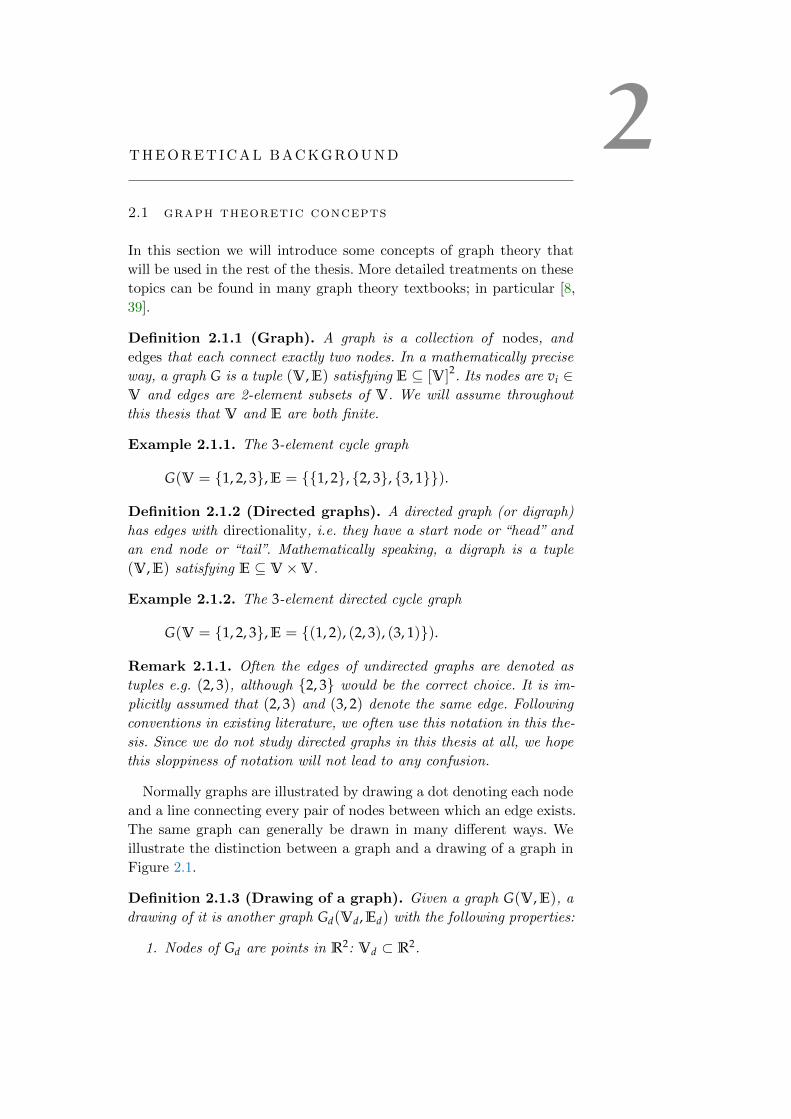
Definition 2.1.1 (Graph). A graph is a collection of nodes, and
edges that each connect exactly two nodes. In a mathematically precise
way, a graph G is a tuple (V, E) satisfying E ⊆ [V]2. Its nodes are vi ∈V and edges are 2-element subsets of V. We will assume throughout
this thesis that V and E are both finite.
Example 2.1.1. The 3-element cycle graph
G(V = 1, 2, 3, E = 1, 2, 2, 3, 3, 1).
Definition 2.1.2 (Directed graphs). A directed graph (or digraph)
has edges with directionality, i.e. they have a start node or “head” and
an end node or “tail”. Mathematically speaking, a digraph is a tuple
(V, E) satisfying E ⊆ V×V.
Example 2.1.2. The 3-element directed cycle graph
G(V = 1, 2, 3, E = (1, 2), (2, 3), (3, 1)).
Remark 2.1.1. Often the edges of undirected graphs are denoted as
tuples e.g. (2, 3), although 2, 3 would be the correct choice. It is im-
plicitly assumed that (2, 3) and (3, 2) denote the same edge. Following
conventions in existing literature, we often use this notation in this the-
sis. Since we do not study directed graphs in this thesis at all, we hope
this sloppiness of notation will not lead to any confusion.
Normally graphs are illustrated by drawing a dot denoting each node
and a line connecting every pair of nodes between which an edge exists.
The same graph can generally be drawn in many different ways. We
illustrate the distinction between a graph and a drawing of a graph in
Figure 2.1.
Definition 2.1.3 (Drawing of a graph). Given a graph G(V, E), a
drawing of it is another graph Gd(Vd, Ed) with the following properties:
1. Nodes of Gd are points in R2: Vd ⊂ R2.
16 theoretical background
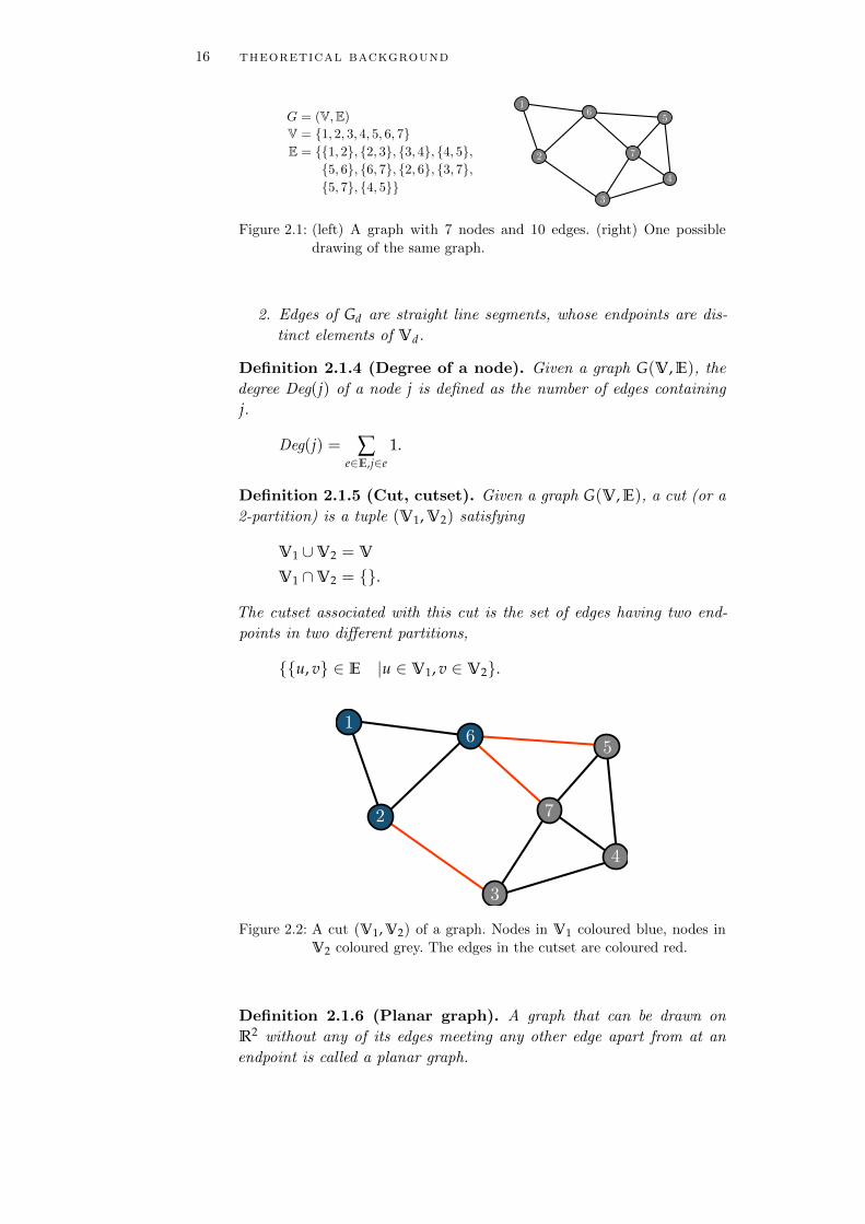
Figure 2.1: (left) A graph with 7 nodes and 10 edges. (right) One possible
drawing of the same graph.
2. Edges of Gd are straight line segments, whose endpoints are dis-
tinct elements of Vd.
Definition 2.1.4 (Degree of a node). Given a graph G(V, E), the
degree Deg(j) of a node j is defined as the number of edges containing
j.
Deg(j) = ∑e∈E,j∈e
1.
Definition 2.1.5 (Cut, cutset). Given a graph G(V, E), a cut (or a
2-partition) is a tuple (V1, V2) satisfying
V1 ∪V2 = V
V1 ∩V2 = .
The cutset associated with this cut is the set of edges having two end-
points in two different partitions,
u, v ∈ E |u ∈ V1, v ∈ V2.
Figure 2.2: A cut (V1, V2) of a graph. Nodes in V1 coloured blue, nodes in
V2 coloured grey. The edges in the cutset are coloured red.
Definition 2.1.6 (Planar graph). A graph that can be drawn on
R2 without any of its edges meeting any other edge apart from at an
endpoint is called a planar graph.

2.1 graph theoretic concepts 17
Figure 2.3: A 4-node planar graph with two different drawings. In the drawing
on the left, two edges intersect, but not in the drawing on the right.
Remark 2.1.2. A graph can have intersecting edges in a specific draw-
ing and still be planar. One example is the complete 4-node graph illus-
trated in Figure 2.3.
Figure 2.4: A length 3 path P1 = (1, 2, 3, 4) and a length 4 path P2 =(1, 6, 5, 7, 4) between nodes 1 and 4 in a graph. P1 is a shortest
path.
Definition 2.1.7 (Path, path length, shortest path). In a graph
G(V, E), a sequence of distinct nodes P = (u1, u2, · · · , un) is called a
path between the nodes u1 and un if there exists an edge between each
successive pair of nodes in the sequence,
for all 1 ≤ j ≤ n− 1, uj, uj+1 ∈ E, (2.1)
for all 1 ≤ i < j ≤ n, ui 6= uj. (2.2)
The Length of a path P is defined as the length of the sequence P .
A path P = (u1, u2, · · · , un) is called a shortest path between u1 and
un if the length of P is smaller than or equal to the lengths of all other
paths between u1 and un. This is illustrated in Figure 2.4.
Remark 2.1.3. Often in graph theory literature, a sequence of nodes
not satisfying the distinctness condition Eq. (2.2) (i.e. where a node
appears more than once) is also called a path, and a “simple path” refers
to what we call path.
18 theoretical background
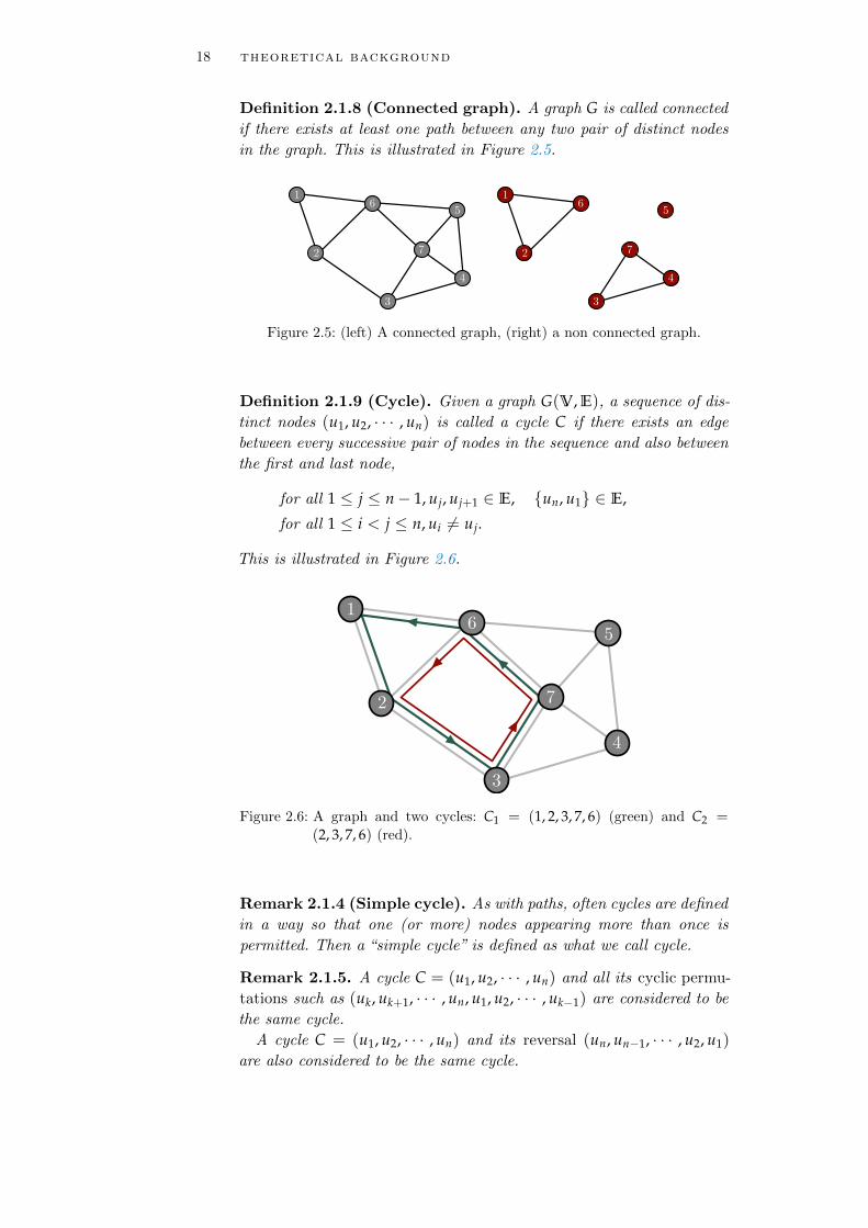
Definition 2.1.8 (Connected graph). A graph G is called connected
if there exists at least one path between any two pair of distinct nodes
in the graph. This is illustrated in Figure 2.5.
Figure 2.5: (left) A connected graph, (right) a non connected graph.
Definition 2.1.9 (Cycle). Given a graph G(V, E), a sequence of dis-
tinct nodes (u1, u2, · · · , un) is called a cycle C if there exists an edge
between every successive pair of nodes in the sequence and also between
the first and last node,
for all 1 ≤ j ≤ n− 1, uj, uj+1 ∈ E, un, u1 ∈ E,
for all 1 ≤ i < j ≤ n, ui 6= uj.
This is illustrated in Figure 2.6.
Figure 2.6: A graph and two cycles: C1 = (1, 2, 3, 7, 6) (green) and C2 =(2, 3, 7, 6) (red).
Remark 2.1.4 (Simple cycle). As with paths, often cycles are defined
in a way so that one (or more) nodes appearing more than once is
permitted. Then a “simple cycle” is defined as what we call cycle.
Remark 2.1.5. A cycle C = (u1, u2, · · · , un) and all its cyclic permu-
tations such as (uk, uk+1, · · · , un, u1, u2, · · · , uk−1) are considered to be
the same cycle.
A cycle C = (u1, u2, · · · , un) and its reversal (un, un−1, · · · , u2, u1)are also considered to be the same cycle.

2.1 graph theoretic concepts 19
Remark 2.1.6 (Edges in a cycle). A cycle C = (u1, u2, · · · , cn)contains n edges (u1, u2, u2, u3, · · · , un−1, un, un, u1). We also
refer to its edge set by the term “cycle”.
Remark 2.1.7 (Symmetric difference between cycles). Given
two cycles C1 and C2 of a graph, the symmetric difference of their edge
sets C1 \ C2 is also a cycle. This is demonstrated in Figure 2.7.
Figure 2.7: Symmetric difference between two cycles (green and red) is also a
cycle (blue).
Definition 2.1.10 (Cycle space, cycle basis). Given a graph G(V, E),
the set of all cycles of the graph C defines a vector space over the two
element finite field Z2. The vector addition between two cycles is the
symmetric difference. The scalar multiplication is defined as
for all C ∈ C, C · 0 = C · 1 = C.
A basis of this cycle space is called a cycle basis BC of the graph. We
illustrate a graph and two cycle bases in Figure 2.8.
Figure 2.8: Two different cycle basis of a graph.
Definition 2.1.11 (Graph incidence matrix). Given a graph G(V, E),
an incidence matrix I for that graph is a |V| × |E| matrix containing
information about which edge connects which pair of nodes. In order to
construct such a matrix, we first impose an arbitrary order on V and
E. Furthermore, for each edge (i, j) we arbitrarily assign an “orienta-

20 theoretical background
tion” by choosing either i or j to be its “head” and the other one to be
its “tail”. Then I is constructed as follows:
Ij,e =
+1 if node j is the head of e = j, `,−1 if node j is the tail of e = j, `,
0 otherwise.
(2.3)
Figure 2.9: (left) a graph and (right) one of the many possible incidence ma-
trices describing the graph. The arrowheads on each edge do not
mean the edge is directed: it just shows the arbitrarily chosen ori-
entation for constructing the incidence matrix.
Remark 2.1.8 (Weighted incidence matrix). For an weighted
graph with edge weights Kij |i, j ∈ E, the weighted incidence ma-
trix Iw is constructed identically to the unweighted incidence matrix,
but the nonzero entries are ±Kij instead of ±1,
Iwj,e =
Kij if node j is the head of e = j, `,−Kij if node j is the tail of e = j, `,
0 otherwise.
(2.4)
Definition 2.1.12 (Laplacian matrix). Given a graph G(V, E), its
Laplacian matrix L is a V×V matrix. To construct it, we first need
to impose an arbitrarily chosen order on V, just as in definition 2.1.11.
Then L is defined as
Li,j =
Deg(i) if i = j,
−1 if i 6= j and (i, j) ∈ E,
0 otherwise.
(2.5)
Remark 2.1.9 (Weighed Laplacian matrix). For an weighted graph
with edge weights Kij |i, j ∈ E, the weighted incidence matrix Lw
is defined as
Li,j =
∑
k∈V,i,k∈E
Kik if i = j,
−Kij if i 6= j and (i, j) ∈ E,
0 otherwise.
(2.6)

2.2 flow networks 21
2.2 flow networks
Definition 2.2.1 (Flow). Given a graph G(V, E), a flow F on it is
defined as a mapping, that associates to each vertex pair (i, j) connected
by an edge e a real number Fij denoting a “flow” from j to i.
F : (i, j) | i, j ∈ E →R
: (i, j) 7→Fij.(2.7)
Definition 2.2.2 (Flow network). Given a graph G and a flow Facross its edges, the tuple (G,F ) is called a flow network.
Remark 2.2.1 (Directionality of flows). We implicitly assume Fij =
−Fji. This is consistent with the intuitive notion of flows being directed
quantities: flow from a to b must be opposite in sign and equal in mag-
nitude to the flow from b to a.
Remark 2.2.2 (Flow vector). Often it is useful to treat a flow as a
|E| element vector F. Such a vector contains the same information as
the mapping F itself and is constructed as follows.
Consider a specific ordering of the edge set E =
e1, e2, · · · , e|E|
and
a specific orientation of the edges (see definition 2.1.11) of G. Then the
flow vector is
F =(
F1, F2, · · · , F|E|)
(2.8)
Fk =
Fij if i is the head of ek
−Fij if j is the head of ek.(2.9)
Definition 2.2.3 (Conservative flow). If a flow from i to j is a
monotonically increasing, continuous and differentiable function of the
difference between certain vertex property across the edge i, j,
Fij = Kij f (ϕj − ϕi) (2.10)
Φ : V→ RV (2.11)
: vj 7→ ϕj (2.12)
f : R → R (2.13)
f (y) > f (x)⇔ y > x, (2.14)
then it is called a conservative flow.
Remark 2.2.3. To satisfy the flow directionality condition (see remark
2.2.1), f must be an odd function
f (−x) = − f (x).
Remark 2.2.4 (Flow continuity/Kirchoff’s law). Often, flows are
quantities that enter or exit a graph at certain nodes and their total

22 theoretical background
quantity follows a certain conservation law called Kirchoff’s law. Defin-
ing a vertex property called input Ij ∈ R for all nodes j, this law states
Ij + ∑(j,l)∈E
Fjl = 0. (2.15)
Definition 2.2.4 (Conservative flow network). Let G be a graph
with inputs Ij at each node j. Let F be a conservative flow satisfying the
flow continuity condition Eq. (2.15). Then the tuple (G, I,F ) is called
a conservative flow network.
Now we will give two examples of conservative flow networks: first,
Kuramoto oscillator networks, and second, linear flow networks.
2.2.1 Kuramoto networks
Kuramoto model [1] describes phase oscillators coupled to each other
by sinusoidal couplings. This model has been used to study the collec-
tive dynamics of coupled Josephson junctions [15], neuronal networks
[16], chemical oscillators [17], and a variety of other synchronization
phenomena [4, 2, 40, 41].
This system is described by an undirected graph G with N nodes and
M edges. Each node is a phase oscillator with natural frequencies θj, j ∈1, 2, · · · , N. Each edge i, j has an associated coupling strength Kij >
0. The phase variables in this system are the phase angles of each node
θj, j ∈ 1, 2, · · · , N, and the equations of motion are given by
dθj
dt= ωj + ∑
(i,j)∈E
Kij sin(θi − θj
), (2.16)
for all 1 ≤ j ≤ N. By construction, Kji = Kij.
Kuramoto model as a flow network
The steady state of a Kuramoto network is defined by phase angles
θ∗1 , θ∗2 , · · · , θ∗N satisfying
ωj + ∑i,j∈E
Kij sin(θi − θj
)= 0, for all 1 ≤ j ≤ N. (2.17)
Such a steady state describes a flow (see definition 2.2.1),
Fkuram : (i, j) | i, j ∈ E →R (2.18)
: (i, j) 7→Kij sin(θi − θj
). (2.19)
We see from Eq. (2.17) that Fkuram satisfies the flow conservation
condition Eq. (2.15). Thus a steady state of Kuramoto oscillator net-
works defines a conservative flow network(G, ω,Fkuram
).
2.2 flow networks 23
2.2.2 Linear flow networks
If in a flow network, the flows across each edge is proportional to certain
potential difference across each edge, then it is called a linear flow
network. Such networks are encountered in various systems such as
incompressible fluid flow in pipes [42, 43], DC flow in resistor networks
[44] as well as flow of sap in plant leaves [14].
Such networks consist of inputs Ij at each node i ∈ V. Each edge is
defined to have a certain conductivity Kij and the flows in such networks
are given by
F linear : (i, j) | i, j ∈ E →R (2.20)
: (i, j) 7→Kij(
ϕi − ϕj)
, (2.21)
satisfying the flow continuity condition Eq. (2.15)
Ij + ∑i,j∈E
Kij(
ϕi − ϕj)
= 0.
Thus(G, I,F linear
)defines a conservative flow network.


3C O N N E C T I N G T H E D O T S
In Chapter 1, we motivated the topic of this thesis: “dynamics of com-
plex flow networks”. In Chapter 2, we introduced the tools and concepts
we will be using. Here we will connect the dots between the different
open problems motivating this thesis, put them in the context of ex-
isting research and explain in detail our approaches in solving these
problems.
3.1 topology dependence of steady flows and their
stability
For proper functioning of a flow network, often it is desirable that the
flows across the edges are stationary (i.e. they do not change with time,
barring external perturbations). For instance, in AC power grids, the
loss of such stationary (or steady) states results in a power outage.
Therefore, it is of paramount importance to understand under which
conditions such steady states exist, under which conditions they are sta-
ble, and which topological features help to achieve these steady states.
In the context of Kuramoto networks, it was reported by Kuramoto
himself [1] that for all-to-all coupled networks in the limit of infini-
tel system size, the answer to this question is simple: if the coupling
strength is below some critical coupling Kc, there exists no steady state,
and otherwise there exists a unique globally attracting steady state
(Here we emphasize again that by the term “steady state” we refer to
a globally phase locked state where all oscillators rotate with the same
frequency. We do not distinguish between the “partially phase locked”
and the “unsynchronized” state as they are often called in classic Ku-
ramoto literature because none of them have steady flows and hence
are equally“unsynchronized” from the flow dynamics perspective). This
critical coupling is easily obtained from the distribution of natural fre-
quencies of the oscillators (or power injections in the analogous AC
power grid model): if the frequencies are all very close the average
value, critical coupling is low; but if they have a “wider” distribution,
critical coupling is high. Unfortunately, such necessary and sufficient
conditions for steady states in general topology Kuramoto networks
have not been found to date.
We know that the critical coupling strength can no longer be com-
puted from the statistical distribution of oscillator frequencies alone,
since the topological distribution of the oscillators (i.e. of their natu-
ral frequencies) matter, as do the connectivity pattern of individual
nodes. Therefore, graph theoretic notions such as node degree distri-
26 connecting the dots
bution [22], clustering coefficient [24] and global graph partitions [45]
have been invoked to determine the critical coupling.
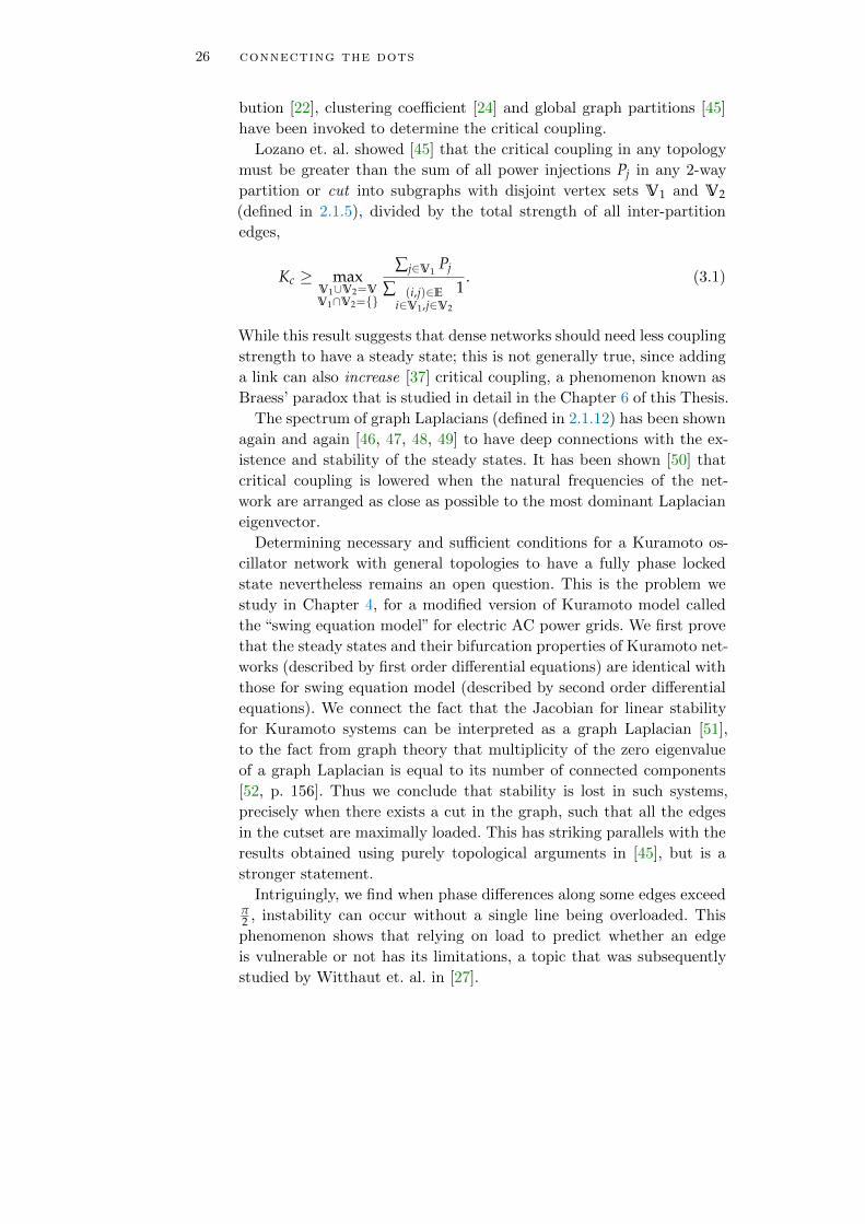
Lozano et. al. showed [45] that the critical coupling in any topology
must be greater than the sum of all power injections Pj in any 2-way
partition or cut into subgraphs with disjoint vertex sets V1 and V2
(defined in 2.1.5), divided by the total strength of all inter-partition
edges,
Kc ≥ maxV1∪V2=VV1∩V2=
∑j∈V1Pj
∑ (i,j)∈Ei∈V1,j∈V2
1. (3.1)
While this result suggests that dense networks should need less coupling
strength to have a steady state; this is not generally true, since adding
a link can also increase [37] critical coupling, a phenomenon known as
Braess’ paradox that is studied in detail in the Chapter 6 of this Thesis.
The spectrum of graph Laplacians (defined in 2.1.12) has been shown
again and again [46, 47, 48, 49] to have deep connections with the ex-
istence and stability of the steady states. It has been shown [50] that
critical coupling is lowered when the natural frequencies of the net-
work are arranged as close as possible to the most dominant Laplacian
eigenvector.
Determining necessary and sufficient conditions for a Kuramoto os-
cillator network with general topologies to have a fully phase locked
state nevertheless remains an open question. This is the problem we
study in Chapter 4, for a modified version of Kuramoto model called
the “swing equation model” for electric AC power grids. We first prove
that the steady states and their bifurcation properties of Kuramoto net-
works (described by first order differential equations) are identical with
those for swing equation model (described by second order differential
equations). We connect the fact that the Jacobian for linear stability
for Kuramoto systems can be interpreted as a graph Laplacian [51],
to the fact from graph theory that multiplicity of the zero eigenvalue
of a graph Laplacian is equal to its number of connected components
[52, p. 156]. Thus we conclude that stability is lost in such systems,
precisely when there exists a cut in the graph, such that all the edges
in the cutset are maximally loaded. This has striking parallels with the
results obtained using purely topological arguments in [45], but is a
stronger statement.
Intriguingly, we find when phase differences along some edges exceedπ2 , instability can occur without a single line being overloaded. This
phenomenon shows that relying on load to predict whether an edge
is vulnerable or not has its limitations, a topic that was subsequently
studied by Witthaut et. al. in [27].

3.2 multistability and topology 27
3.2 multistability and topology
We noted in Section 3.1 that all-to-all coupled Kuramoto networks have
either one or no steady states in the infinite system size limit. For
power grid operation, this is a very desirable property: given a fixed
distribution of power injections at the nodes, each edge is guaranteed
to carry a fixed amount of flow, independent of initial conditions or
temporary perturbations in the grid. The problem is, power grids are
almost never all-to-all coupled. In fact, they tend to be planar or almost
planer [20, 21]. Taylor [29] showed that uniqueness of steady states holds
also in non all-to-all coupled systems as long as the network is denser
than a certain limit. It has been claimed in a highly cited article [28]
that for any Kuramoto network there always exists a certain coupling
strength, above which uniqueness of steady states is guaranteed.
However, this claim contradicts results demonstrating multistability
[30, 53] in Kuramoto systems. As one core contribution of this thesis,
we identified a flaw the proof in [28], at an application of Banach’s con-
traction principle. As a consequence, high coupling strength happens
to increase the number of steady state, rather that decreasing it to one.
It had already been shown [30] that in ring topologies the number
of steady state scales linearly with ring size. Such states, containing
twisted phase angles, were postulated [53] to have basin volumes de-
creasing with the amount of “twist” quantified in a so-called winding
number. Interestingly, it is known that a unique steady state exists
for both the sparsest (i.e. tree) and densest (i.e. all-to-all connected)
topologies [54], but not for intermediately dense ones. Research con-
ducted parallely and independently from our thesis work showed [55]
in 2016 that the number of steady states increase with loop lengths of
the network in plane embedded Kuramoto networks with identical fre-
quencies. However, counting the number of steady states in Kuramoto
networks with general topologies and general natural frequency distri-
bution is still an unsolved problem.
In Chapter 5, we demonstrate that the number of coexisting steady
flow in planar Kuramoto networks increase with coupling strengths of
the edges, length of fundamental cycles as well as the spatial homogene-
ity of the natural frequencies. For large network size and large coupling
strength, we derive a scaling law for the number of steady states. We
numerically show that the said scaling matches very well with reality
(for cycle lengths as low as 50), as opposed to previously known upper
bounds, which were much higher than the actual numbers.
3.3 topological perturbations and steady flows
Flow networks are often subjected to topological perturbations, both
planned and unplanned. Examples include shutdown of power lines
due to a storm or scheduled maintenance; or leaf veins being eaten

28 connecting the dots
through by bugs. Resilience against such perturbations is therefore a
very desirable property for flow networks. Indeed, electrical power grids
are supposed to fulfill the “n− 1 criteria” mandating that there should
be no blackout due to the shutdown of any one power line at a time.
Nevertheless, topological perturbations sometimes cause other lines
to fail, resulting in collective failures of big parts of the grid [56, 57].
Indeed, in 2006 shutdown of a single power line in the Ems river in
northern Germany, done intentionally in order to let a ship pass, re-
sulted in a continent wide blackout reaching up to Spain [57].
As a result, understanding, predicting and preventing such failures
is an important issue that has been approached from various different
directions in the past. Attempts to establish correlation between vulner-
ability of edges and their topological properties indicate that decentral
power grids [26] are more robust against topological damages. Nodes
with higher degrees seem to be crucial for stable operation, as a result
scale free networks have been numerically shown [58] to be vulnerable
to deliberate sabotage targeting their hubs. Intentionally cutting trans-
mission lines have been demonstrated [59] to be sometimes effective in
preventing cascading failures. In a different context, leaf venation net-
works with more cycles were shown [14] to be robust against topological
perturbation compared to leaves with less cycles.
How steady flows are affected by damage or removal of an edge in a
flow network is still not well understood. We will now describe a specific
aspect of this issue that we studied in this thesis: the so called “Braess’
paradox”.
3.3.0.1 Braess’ paradox
Figure 3.1: Braess’ paradox as reported by D. Braess. (Left) A four edge net-
work has two edges with travel time proportional to the number
of cars in it. In the other two edges, travel time is constant. Each
car chooses the shortest path selfishly. With total 4000 cars in the
network, each takes 65 minutes to reach its destination. (Right)
Opening a new zero travel time edge causes all cars to take 80minutes to reach their destinations.
In the context of traffic networks, a curious phenomenon was reported
in 1968 (illustrated in Figure 3.1), where opening a new street led to
3.4 summary 29
increased travel time for every car [32]. Later, the same phenomenon,
termed Braess’ paradox, has been observed in the context of other flow
networks like AC and DC power grids [36, 37, 38]. Braess’ paradox
can cause undesirable flow patterns and potentially instabilities in flow
networks if not properly accounted for, because adding new edges or
strengthening existing ones is a very common strategy to compensate
for increased load in flow networks. Despite extensive research [60, 35,
61] on the topic, the question of which edges in a flow network will
exhibit Braess’ paradox, remains unanswered to date.
In Chapter 6, we systematically study the phenomenon of Braess’
paradox in a class of continuous flow networks we call conservative
flow networks (defined in 2.2.4), which includes both Kuramoto net-
works and leaf venation networks in plants, among other systems. We
take a differential view to Braess’ paradox: We define an edge to be
Braessian if infinitesimal increase in its strength results in the maxi-
mum flow in the network increasing. We first derive an exact mapping
from the problem of detecting Braessian edges to computing steady
state flows in a modified “meta graph” of residual capacities with only
one dipole source. This boils down to solving Laplace equation with a
single dipole source in a weighted graph (continuum variant of which
is very familiar from electrostatics). Guided by this insight, we define
an intuitive notion of flow alignment, and demonstrate that edges with
flows aligned to the maximally loaded edge are more likely to be Braes-
sian. We build and test three classifiers to detect Braessian edges. The
first one, based on edge distances, is applicable to any graph and com-
putationally fast; but error prone. The second one is based on distances
in dual graphs, and consequently applicable only to plane graphs; but
with significantly more accurate than the first one. We propose a third
classifier based on rerouting pathways in the graph, that performs as
well as the second one, and at the same time applicable to non-planar
graphs as well. The only disadvantage of this classifier is high compu-
tational complexity. Last, we demonstrate that Braess’ paradox has a
very beneficial effect: Braessian edges can be intentionally damaged to
mitigate overload caused by damage at another edge.
3.4 summary
In this thesis, we studied three aspects of the general question: how
does network topology influence the dynamics of flow networks? In
Chapter 4, we derive equivalence of steady states (and their bifurca-
tions) between Kuramoto oscillators and the swing equation model of
AC power grid. We map loss of stability in these two systems to graph
theoretic notion of connectedness. In Chapter 5, we demonstrate how
the number of steady states in the same system increases with three
topological properties – namely number of fundamental cycles, coupling
strength at the edges and spatial homogeneity of natural frequencies.

30 connecting the dots
In Chapter 6, we demonstrate that we can predict Braessian edges in
a conservative flow network from topological features of the edges, and
show that Braess’ paradox can be put to good use to mitigate overload
in a flow network. In Chapter 7, we summarize our results and identify
future research directions.

4A RT I C L E – S U P P LY N E T WO R K S : I N S TA B I L I T I E S
W I T H O U T OV E R L OA D
Debsankha Manik1,4, Dirk Witthaut a1,4, Benjamin Schafer1,3, Moritz
Matthiae1, Andreas Sorge1, Martin Rohden1, Eleni Katifori1,2, Marc
Timme1,2
1 Network Dynamics, Max Planck Institute for Dynamics and Self-
Organization (MPI DS), 37077 Gottingen, Germany
2 Faculty of Physics, University of Gottingen, 37077 Gottingen,
Germany
3 Otto-von-Guericke-Universitat Magdeburg, 39106 Magdeburg, Ger-
many
4 These authors contributed equally to this work.
Published in:
The European Physical Journal Special Topics 223 (12) 2014:
2527-2547
DOI (for Published version):
10.1140/epjst/e2014-02274-y
Legal note:
Reprinted with permission from EDP Sciences, Springer-Verlag.
The final publication is available at link.springer.com.
Original contribution:
I carried out most of the analytical calculations behind the results,
contributing almost all the results in Sec 3 and 5, as well as interpreta-
tion and analytical calculations for results in Sec 6.1 and 6.2. I wrote
significant parts of all the text sections, except Sec 4. I revised the
manuscript during revision process, updating texts and figures as per
referee reports.
a Current address: Forschungszentrum Julich, Institute for Energy and Climate Re-
search (IEK-STE), 52425 Julich, Germany; e-mail: [email protected]
32 article – supply networks: instabilities without overload
Abstract. Supply and transport networks support much of our
technical infrastructure as well as many biological processes. Their
reliable function is thus essential for all aspects of life. Transport
processes involving quantities beyond the pure loads exhibit alterna-
tive collective dynamical options compared to processes exclusively
characterized by loads. Here we analyze the stability and bifurcations
in oscillator models describing electric power grids and demonstrate
that these networks exhibit instabilities without overloads. This phe-
nomenon may well emerge also in other sufficiently complex supply or
transport networks, including biological transport processes.
4.1 introduction
Today’s society depends on the reliable supply of electric power. The
Energy transition to renewable energy (Energiewende) impairs the con-
ventional power distribution system and poses great challenges for the
security of the energy supply [62, 63]. It has been shown by Pesch et
al. [64] that the grid might become more heavily loaded in the future
as electric power generation varies over time and has to be transported
over large distances. For instance, current planning assigns new large-
distance distribution lines from off-shore wind parks to the inner land
– making the grid more susceptible to perturbations. Moreover, wind
turbines and photovoltaic arrays are strongly intermittent; their power
output fluctuates on all timescales from years to below seconds [65, 66,
67]. To ensure continued stable operation of power grids, it is advisable
to understand how the network structure of the power grid determines
its dynamic stability and how instabilities generally emerge.
4.2 an oscillator model for power grid operation
In this article we analyze network models of power grids consisting of
rotating machines representing electric generators and motors. These
models describe the phase dynamics of the machines and thus cap-
ture important problems of synchronization and dynamical stability
of complex power grids [68, 69, 19, 70] and have recently attracted
considerable interest in physics and mathematics [26, 36, 71, 49, 72,
73]. Notably, these models are mathematically very similar to the cele-
brated Kuramoto model describing the dynamics of coupled limit cycle
oscillators [1, 4, 2].
Variations of these models are widely used in power engineering [68,
69, 74, 70, 75, 76]. In many of the applications, however, passive loads
are considered instead of motors which can be eliminated via a Kron
reduction [77]. The resulting model is mathematical equivalent to the
one analyzed here, but its dimension is typically significantly smaller
after this reduction (see Section 4.2.2 for details).

4.2 an oscillator model for power grid operation 33
4.2.1 The oscillator model
We model the power grid as a network of N rotating machines rep-
resenting, for instance, wind turbines or electric motors [19, 26]. Let
the machines be denoted by a natural number j ∈ ZN where ZN =
1, 2, · · · , N. Each machine j is characterized by the mechanical power
Pmechj it generates (Pmech
j > 0) or consumes (Pmechj < 0). The state
of each rotating machine is determined by its mechanical phase angle
φj(t) and its velocity dφj/dt. During the regular operation, genera-
tors as well as consumers within the grid run with the same frequency
Ω = 2π× 50Hz (Europe) or Ω = 2π× 60Hz (USA). The phase of each
element j is then written as
φj(t) = Ωt + θj(t), (4.1)
where θj denotes the phase difference to the reference value Ωt.The equations of motion for all θj can now be obtained from the
energy conservation law, i.e. the generated energy Pmechj of each single
element must equal the accumulated and dissipated mechanical energy
of this machine plus the electric energy Pelj transmitted to the rest of
the grid. We also have
Pdissj = Dj(φj)
2 (4.2)
Paccj =
12
Ijddt
(φj)2, (4.3)
where Ij is the moment of inertia and Dj is the damping torque. The
energy conservation law reads
Pmechj = Pdiss
j + Paccj + Pel
j . (4.4)
We will now insert equation (4.1) in the formula for the accumulated
and dissipated mechanical energy to derive the equations of motion. In
the vicinity of the regular operation of the grid, phase changes are small
compared to the reference frequency [19] |θj| Ω and we can write
the equations of motion for θj as
∀j ∈ ZN , IjΩθj = Pmechj − DjΩ2 − 2DjΩθj − Pel
j . (4.5)
The electric power is determined as follows. In a synchronous machine
with p f number of poles, the phase φj of the AC electric voltage and
the mechanical phase φmechj have a fixed ratio [74, p. 47]
φj =p f
2φmech
j .
We here consider common two-pole machines where this ratio is unity,
i.e. φj(t) = φmechj (t).
In an AC circuit, where the current between two nodes Iij and voltage
at jth node Vj vary sinusoidally with a relative phase difference δ, the
power transmitted from node j to node i is
Pij(t) = Vj(t)Iij(t) (4.6)

34 article – supply networks: instabilities without overload
=(
Vj,rms
√2)
sin (Ωt)(
Iij,rms
√2)
sin (Ωt + δ) (4.7)
= Vj,rms Iij,rms cos δ︸ ︷︷ ︸Pij,real
−Vj,rms Iij,rms cos (2Ωt + δ). (4.8)
The second term oscillates between positive and negative values such
that the direction of power flow changes direction. The net flow due to
this term, when integrated over a full period of the AC cycle, is zero.
Since here we consider dynamics on time scales much larger than a
time period of the AC cycle (1/Ω), we ignore this second term. The
first term constitutes the real power flow from generator to consumers.
It is convenient to adopt complex notation at this point:
Vj = Vj,rmseiΩt , Iij =Iij,rmsei(Ωt+δ), (4.9)
such that the apparent and the real power reads
Sij = Vj I∗ij , Pij,real =<(Sij). (4.10)
The net electric power at node j: Pelj in (4.5) is basically the total
Preal transmitted to all neighbouring nodes:
Pelj =
N
∑k=1
Pkj,real (4.11)
= <[
Vj
N
∑k=1
I∗kj
](4.12)
Ikj = Ykj(Vk − Vj). (4.13)
For simplicity we here neglect ohmic losses in the grid such that
the admittance is purely imaginary, Yjk = iBjk. Furthermore, we as-
sume that the magnitude of the voltage is constant throughout the
grid, |Vj| = V0 for all nodes j ∈ ZN. Then Pelj simplifies to
Pelj = <
[N
∑k=1
V20 Bjk
sin(θj − θk) + i
(cos(θj − θk)− 1
)](4.14)
=N
∑k=1
V20 Bjk sin(θj − θk). (4.15)
Substituting this result into equation (4.5) thus yields the equations of
motion
IjΩd2θj
dt2 + Djdθj
dt= Pmech
j − DjΩ2 +N
∑k=1
V20 Bjk sin(θk − θj). (4.16)
The same equations of motions constitute the so-called structure-preserving
model in power engineering [68], which is derived under slightly differ-
ent assumptions.

4.2 an oscillator model for power grid operation 35
For the sake of simplicity we introduce the abbreviations
Pj =Pmech
j − DjΩ2
IjΩ(4.17)
αj =Dj
IjΩ(4.18)
Kjk =V2
0 Bjk
IjΩ(4.19)
such that the equations of motion read
∀j ∈ ZN ,d2θj
dt2 = Pj − αjdθj
dt+ ∑
kKjk sin(θk − θj). (4.20)
In this formulation the regular operation of the grid corresponds to a
stable fixed point with dθj/dt = 0 for all nodes j.Throughout this paper we assume that the network defined by the
coupling matrix is globally connected. Otherwise we can simply con-
sider each connected component separately. We take symmetric trans-
mission capacities
Kjk = Kkj (4.21)
for all j, k as appropriate for (electric) supply networks and Kjj = 0. Fur-
thermore, we assume that the power in the grid is balanced, i.e. ∑j Pj =
0. This is appropriate since we focus on the short-time dynamics of the
grid and the stability of steady states. On longer time-scales, the power
balance is maintained by the grid operators by adapting the generation.
4.2.2 Ohmic loads and the classical model
The oscillator model introduced above assumes that all nodes of the
network represent synchronous machines. In contrast, the so-called clas-
sical model widely studied in power engineering [70] includes a set of
synchronous generators as above, but considers only ohmic loads. The
load nodes of the network can then be eliminated which yields a much
lower dimensional dynamical system. The resulting equations of mo-
tion are mathematically equivalent such that all our results equally
well apply to the classical model. However, the network topology is no
longer obvious in this model as the effective coupling matrix of the
generator nodes is generally non-zero everywhere. Bergen and Hill [68]
rectified this issue by introducing the structure preserving model, which
also gives rise to equations of motion formally identical to the oscillator
model. We thus focus on the oscillator model in the rest of the paper.
In the following we briefly summarize the derivation of the classical
model [77] to show how to deal with ohmic loads in this framework.
We divide the nodes of the networks into active and passive nodes,
where the passive ones represent ohmic loads. For the sake of simplicity

36 article – supply networks: instabilities without overload
we label the nodes such that j = 1, . . . , L are the active nodes and
k = L + 1, . . . , N are the passive nodes. The passive nodes have a fixed
power consumption
Sj = Vj
N
∑k=1
I∗kj︸ ︷︷ ︸=: I∗j
. (4.22)
Even more, one assumes that both factors Vj and Ij are fixed indepen-
dently. One can then eliminate these nodes via a Kron reduction as
follows.
One starts with Kirchhoff’s equations in the form (cf. equation 4.13)
Ij =N
∑k=1
Ijk = ∑k
Yjk(Vk − Vj) = ∑k
QjkVk, (4.23)
where
Qjk = Yjk − δjk ∑`Yj` (4.24)
is called the nodal admittance matrix. These equations are recast into
matrix form(Ia
Ip
)=
(Qaa Qap
Qpa Qpp
)(V a
V p
), (4.25)
where the vectors Ia and Ip collect the currents at the active and the
passive nodes, respectively. These equations are solved for the currents
Ia = (QapQ−1pp )︸ ︷︷ ︸
=:Qac
Ip + (Qaa −QapQ−1pp Qpa)︸ ︷︷ ︸
=:Qred
V a (4.26)
at the active nodes. The net electric power at one of the active nodes
then reads
Sj = Vj
L
∑`=1
Qred∗j` V∗` + Vj
N
∑`=L+1
Qac∗j` I∗` . (4.27)
The second term is fixed by assumption, such that it can be transfered
to the effective mechanical power of the respective node,
Peffj = Pmech
j −<[
Vj
N
∑`=L+1
Qac∗j` I∗`
]. (4.28)
Assuming again that the lines are lossless such that
Yjk = iBjk and Qred∗j` = iBred
j` , (4.29)
4.3 the nature and bifurcations of steady states 37
the equations of motion for the active nodes are then derived from the
energy conservation equation (4.4)
IjΩd2θj
dt2 + Djdθj
dt= Peff
j − DjΩ2 +L
∑`=1
V20 Bred
j` sin(θ` − θj). (4.30)
This is fully equivalent to the equations of motion for the oscillator
model (4.16) such that all mathematical results obtained in the present
article can thus be directly applied to the classical model as well.
4.2.3 Further generalisations
Both the oscillator and the classical model describe only the phase
dynamics of the synchronous machines, assuming a constant voltage
throughout the grid. Several important aspects of the voltage dynamics
in a complex power grid are described by the so-called third-order model
[70]. A recent theoretical study of voltage instabilities can be found in
[78]. Still, all these models neglect Ohmic losses of the transmission
lines. If Ohmic losses are included, the equations of motion become
significantly more complex [70].
4.3 the nature and bifurcations of steady states
During steady operation of a power grid all nodes run with the grid’s
reference frequency Ω and fixed phase differences. A stable fixed point
(i.e. equilibrium/steady state) of the equations of motion (4.20) de-
scribes the steady operation of the power grid. The loss of such a fixed
point or a dynamical instability induce a desynchronization of the grid.
Therefore, it is essential to understand the properties of the fixed points
of the oscillator model, in particular their bifurcations and dynamical
stability.
The fixed points of the equations of motion (4.20) are determined by
the nonlinear algebraic equations
∀j ∈ ZN , Pj + ∑k
Kjk sin(θ∗k − θ∗j ) = 0. (4.31)
In the following, we present several results on the existence, stability
and bifurcations of these fixed points, some aspects of which have been
published for related systems in [79]. Fixed points are marked by an
asterisk and the vector θ = (θ1, . . . , θN)T ∈ SN collects the phases of
all machines, where S = x |0 ≤ x ≤ 2π . The local frequencies are
referred to by vj = dθj/dt or v = dθ/dt, respectively.
Lemma 4.3.1. The network dynamics of the system defined by (4.20)
and (4.21) for αj = 0 (zero damping) is a Hamiltonian system of the
form
θj =∂H∂vj
, vj = −∂H∂θj
, (4.32)

38 article – supply networks: instabilities without overload
where the phase θj and the phase velocity
vj = dθj/dt (4.33)
are canonically conjugate variables for all j ∈ ZN. The Hamiltonian
function has the natural form
H(v, θ) = T(v) + V(θ) (4.34)
with the kinetic and potential energies
T(v) =12 ∑
jv2
j (4.35)
V(θ) = −∑j
Pjθj −12 ∑
i,jKij cos(θi − θj). (4.36)
Proof. Let H(v, θ) = T(v) + V(θ) be a Hamiltonian function defined
by (4.34), (4.35) and (4.36). Then H is continuously differentiable on
any open star-shaped subset of the phase space with
∂H/∂vj = vj = θj (4.37)
and
∂H∂θj
= −Pj −12 ∑
k∑
lKkl
∂
∂θjcos(θk − θl) (4.38)
= −Pj −∑k
Kjk sin(θk − θj). (4.39)
Where the last equality follows from symmetry (4.21). Substituting
(4.33), (4.37) and (4.39) into the Hamilton equations (4.32), the claim
follows.
Corollary 4.3.1. The set of all fixed points of the oscillator equation
(4.20) and (4.21) for arbitrary αj ∈ R, j ∈ ZN, is identical to the set
of fixed points of the Hamiltonian system (4.32) with (4.34) and (4.33).
The fixed points are local extrema/saddle points of the potential function
V(θ) (cf. also [80]).
Proof. The set of fixed points of (4.32) is given by
PHamilton =
(θ∗, v∗)
∣∣∣∣∀j ∈ ZN ,∂H∂vj
= 0∧−∂H∂θj
= 0
(4.40)
The set of fixed points of the oscillator equations (4.20) is given by
Posc =
(θ∗, v∗) = (θ∗, 0)
∣∣∣∣∣∀j ∈ ZN , Pj +N
∑k=1
Kjk sin(θ∗k − θ∗j ) = 0
,
(4.41)
4.3 the nature and bifurcations of steady states 39
independent of all αj. If the transmission capacities are symmetric
(4.21), the Hamiltonian and the original oscillator dynamics in the αj =
0 case are equivalent (have identical trajectories) as ensured by Lemma
4.3.1. Thus in particular their fixed points are identical. And since the
fixed points of the oscillator model don’t depend on αj as per (4.41),
the fixed points of the oscillator model for arbitrary αj are also, by
extension, identical to those of the Hamiltonian system.
As T(v) is independent of all θj we have at each fixed point (θ∗, v∗)that
∂H(v, θ)
∂θj
∣∣∣∣θ∗
=∂V(θ)
∂θj
∣∣∣∣θ∗
= 0 (4.42)
for all j such that the fixed points are located at local extreme/saddle
points of V, demonstrating the second claim.
Because of this correspondence, the theory of (damped) Hamiltonian
dynamical systems (see [81] and references therein) helps us in charac-
terizing the fixed points of the oscillator model and their bifurcations.
We note that one has to be careful about the domain of H. In principle,
the phases are only defined modulo 2π but H is not 2π-periodic. This
fact is not a major problem for our purpose, but it prohibits a definition
of Gibbsian ensembles in statistical mechanics [80, 2].
As shown in Corollary 4.3.1, the location of the fixed points θ∗ =
(θ∗1 , . . . , θ∗N) is independent of the damping coefficients αj. Furthermore,
the location of the fixed point is the same for the celebrated Kuramoto
[1, 4, 2] model such that our results may be adapted for this important
model system. The question naturally arises: how do the stability prop-
erties of the fixed points change when αj are varied or when we go from
the oscillator model to Kuramoto model? We will answer this question
subsequently, in Lemma 4.3.2 and Theorem 4.3.1.
The linear or spectral stability of a fixed point is obtained by lin-
earizing the equations of motion. Writing
ξ = θ− θ∗ (4.43)
the linearized equations of motion are given by
ddt
(ξ
ξ
)= J
(ξ
ξ
). (4.44)
For the given damped oscillator system with equations of motion (4.20),
the Jacobian is given by
J =
(−AN×N −MN×N
IN×N 0N×N
), (4.45)
where
A =
α1 0 · · ·0 α2 · · ·...
.... . .
(4.46)
40 article – supply networks: instabilities without overload
is a diagonal matrix specifying the damping coeeficient at each node
and M is the Hesse matrix of the potential function V(θ) with elements
Mij =∂2V
∂θi∂θj(4.47)
M =
N
∑l=1
K1l cos (θ∗1 − θ∗l ) −K12 cos (θ∗1 − θ∗2 ) · · ·
−K21 cos (θ∗2 − θ∗1 )N
∑l=1
K2l cos (θ∗2 − θ∗l ) · · ·...
.... . .
. (4.48)
This can be verified by a straightforward calculation.
Let λj be the eigenvalues of the Jacobian matrix J:
∀j ∈ 1, 2, . . . , 2N , Jvj = λjvj (4.49)
and let µk be the eigenvalues of the Hesse matrix M:
∀k ∈ 1, 2, . . . , N , Muk = µkuk, (4.50)
then we find the results stated below.
Lemma 4.3.2. If µk ≥ 0 for all k ∈ ZN, then <(λj) ≤ 0 for all
j ∈ 1, 2, . . . , 2N. Moreover, for each vj such that Jvj = 02N, there
exists one and only one uk such that
Muk = 0N (4.51)
vj = (0, 0, · · · , 0︸ ︷︷ ︸0N
, u1, u2, · · · , uN︸ ︷︷ ︸uk
) (4.52)
:= 0N ⊗ uk. (4.53)
Proof. Suppose v = v1 ⊗ v2 ∈ RN ⊗RN is an eigenvector of J with
eigenvalue λ. Then we have:
λv1 = −Av1 −Mv2 (4.54)
λv2 = v1 (4.55)
Substituting (4.55) in (4.54):
0 = Mv2 + λAv2 + λ2v2 (4.56)
0 = v2† Mv2 + v2
† Av2λ + v2†v2λ2 (4.57)
= κ21 + κ2
2λ + κ23λ2, (4.58)
where
κ21 = v2
† Mv2 ≥ 0, (M is positive semi-definite) (4.59)
4.3 the nature and bifurcations of steady states 41
κ22 = v2
† Av2 ≥ 0,(αj ≥ 0
)(4.60)
κ23 = v2
†v2 ≥ 0, (4.61)
such that
λ =−κ2
2 ±√
κ42 − 4κ2
1κ23
2κ23
. (4.62)
This implies <(λ) ≤ 0, which proves the first part of the Lemma.
Moreover, <(λ) = 0 ⇐⇒ κ21 = 0, which happens only if Mv2 = 0.
This can be checked by expanding v2 in the eigenbasis of M. This proves
the second part.
Using the technical results presented above, we now analyze the sta-
bility and bifurcations in more detail. We show that stability is entirely
determined by the Hesse matrix M and independent of the damping co-
efficients αj. In many cases, M can be interpreted as a Laplacian matrix
[52], such that the stability can be analyzed in terms of the topology
of the grid.
Before we proceed, we note that by construction the Hesse matrix Mhas one zero eigenvalue (proof in Corollary 4.A.1) with the eigenvector:
u1 = (1, 1, · · · , 1) (4.63)
Mu1 = 0 (4.64)
For notational convenience we denote the eigenvalues of M sorted in
ascending order of absolute values: 0 = |µ1| ≤ |µ2| ≤ |µ3| ≤ · · · ≤|µN |.
Theorem 4.3.1. Let θ∗ be a fixed point of the oscillator model (4.20).
Then θ∗ + ∆(1, 1, · · · , 1)T is also a fixed point for all ∆ ∈ R. If µj > 0for all j ∈ 2, 3, . . . , N, then the fixed point is transversely asymptoti-
cally stable.
Proof. If µj > 0 for all j ∈ 2, 3, . . . , N, Lemma 4.3.2 shows that the
Jacobian J will have only one zero eigenvalue. We can see from (4.63)
that the eigenvector corresponding to zero eigenvalue is
v∗ = 0N ⊗ (1, 1, · · · , 1). (4.65)
This eigenvector implies that a perturbation around a fixed point in
the direction
∆θ∗j = 0, ∆θ∗j = constant (4.66)
is neutrally stable. However, this is simply due to the fact that the
equations of motion (4.20) remains unchanged on adding a uniform
global shift to the phase angles θj.
42 article – supply networks: instabilities without overload
Since all other eigenvalues of the Jacobian J are less than 0, as guar-
anteed by Lemma 4.3.2, we see that all small perturbations transverse
to the global shift (4.66) decay to zero with time. Transverse asymp-
totic stability therefore follows from the center manifold theorem (cf.
[82]).
Lemma 4.3.3. A stable fixed point of the oscillator model (4.20) can
be lost only via an inverse saddle-node bifurcation where one of the µjas defined in (4.50) becomes zero.
Proof. To analyze the nature of bifurcations consider first the hamilto-
nian limit αj = 0. In a hamiltonian system only two types of bifurcation
are possible when a parameter is varied smoothly [81]: a saddle-node bi-
furcation or a Krein bifurcation. At a Krein bifurcation complex quadru-
plets of eigenvalues emerge. However, this is impossible for the given
dynamical system as eigenvalues of the Jacobian J are always purely
real or purely imaginary for α = 0, as demonstrated in (4.62). Thus the
only possible bifurcation scenario is that of a saddle-node bifurcation.
As the position (Theorem 4.3.1) and stability properties (Lemma 4.3.2)
of fixed points are both independent of αj the bifurcation remains the
same also for the non-Hamiltonian case αj > 0.
We note that in the Hamiltonian limit α = 0 stability always means
neutral stability. A minimum of the potential function V(θ) is an “el-
liptic fixed point” or “center” of the dynamical system as all eigenvalues
of the Jacobian are purely imaginary. For αj > 0 all eigenvalues of the
Jacobian acquire a negative real part, such that the fixed point becomes
asymptotically stable.
We note that Theorem 4.3.1 also implies that the fixed points of the
oscillator model share identical position and linear stability properties
with the famous Kuramoto model [2] because −M happens to be the
Jacobian of the Kuramoto system.
4.4 elementary example
To illustrate the mathematical results of the previous section, we first
consider the simplest non-trivial grid, a two-element system consist-
ing of one generator and one consumer. We assume that the power
is balanced, i.e. −P1 = P2 and damping is uniform, i.e. α1 = α2 = α.
Therefore, θ1 + θ2 = −α(θ1 + θ2) and the mean phase θ1 + θ2 of the grid
reaches a constant value exponentially in time. We thus consider only
the dynamics of the phase difference x = θ2 − θ1. With ∆P = P2 − P1
the equation of motion for this system reads
d2xdt2 = ∆P− α
dxdt− 2K sin(x). (4.67)
As the phase difference is defined modulo 2π, the phase space is
cylindrical, (x, x) ∈ R× 2πS1 (however, for illustration purposes and

4.4 elementary example 43
4. Kriterien der Stabilität
Hiermit ist der Leistungsfluss auf der Verbindungsleitung im stationären Fall direktproportional sowohl zur eingebrachten als auch zur entzogenen Leistung. Deshalbwird die Größe ∆p im Folgenden übertragene Leistung genannt, sofern das Systemden stabilen Bereich nicht verlassen hat.
4.2. Das gekippte periodische Potential
Die Bewegungsgleichung der Phasendifferenz (4.2) kann als die Newton’sche ge-dämpfte Bewegung eines Teilchens in einem gekippten periodischen Potential V (x)veranschaulicht werden:
x = −x − dVdx .
Somit ergibt sich für das Potential (siehe Abb. 4.1):
0 π 2π 3π 4πx
0
−50
−100
V(x
)
(a)
0 π 2π 3π 4πx
(b)
0 π 2π 3π 4πx
0
−50
−100
V(x
)
(c)
0 π 2π 3π 4πx
(d)
Abb. 4.1.: Das Potential V (x) = −∆p x − k cos(x) für k = 10 und unterschiedlicheWerte von ∆p. (a) ∆p = 3, (b) ∆p = 6, (c) ∆p = 9 und (d) ∆p = 12.Die lokalen Minima xmin (grün) und Maxima xmax (rot) sind markiert.Für ∆p ≥ k existieren keine stationären Zustände.
28
Figure 4.1: The tilted washboard potential (4.73) for K = 5 and (a) ∆P = 3,
(b) ∆P = 6, (c) ∆P = 9 and (d) ∆P = 12, respectively. The green
(red) points illustrate the local minima (maxima) of the potential
determining the location of a stable (unstable) fixed point.
for comparing to the Hamiltonian case, it might be helpful to “unravel”
the cylinder, i.e. assume that phases can take arbitrary values in R).
Two fixed points exist for 2K > ∆P. The physical reason is that
a steady operation of the grid is possible only when the transmission
capacity of the line is larger than the power that must be transmitted.
The location of the two fixed points Fk = (x∗, x∗) are specified by the
conditions x∗ = 0, x∗ = 0. The eigenvalues of the Jacobian at these
points are given by
F1 : x∗ = arcsin∆P2K
(4.68)
λ(1)± = −α
2±√(α
2
)2− 2K cos
(arcsin
∆P2K
)(4.69)
F2 : x∗ = π − arcsin∆P2K
(4.70)
λ(2)± = −α
2±√(α
2
)2+ 2K cos
(arcsin
∆P2K
). (4.71)
The fixed point F1 is stable: Depending on α, the eigenvalues are either
both real and negative or complex with negative real values. The fixed
point F2 is a saddle, as λ(1)+ is always real and positive while λ
(1)− is
always real and negative.
At 2K = ∆P these two fixed points vanish in an inverse saddle-node
bifurcation. No steady operation is possible for 2K < ∆P as the load
exceeds the capacity of the link. The nature of this bifurcation becomes
most obvious when we consider the potential function introduced in the
Hamiltonian formulation (4.36). The dynamical system (4.67) can be
viewed as the equation of motion of a mechanical particle moving in a
tilted washboard potential with friction
d2xdt2 = −α
dxdt− dV(x)
dx(4.72)
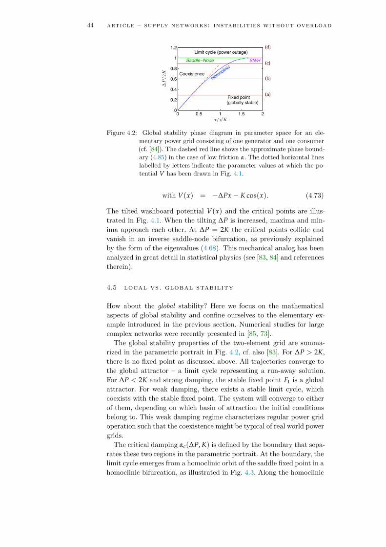
44 article – supply networks: instabilities without overload
(b)
(c)
(d)
(a)
Figure 4.2: Global stability phase diagram in parameter space for an ele-
mentary power grid consisting of one generator and one consumer
(cf. [84]). The dashed red line shows the approximate phase bound-
ary (4.85) in the case of low friction α. The dotted horizontal lines
labelled by letters indicate the parameter values at which the po-
tential V has been drawn in Fig. 4.1.
with V(x) = −∆Px− K cos(x). (4.73)
The tilted washboard potential V(x) and the critical points are illus-
trated in Fig. 4.1. When the tilting ∆P is increased, maxima and min-
ima approach each other. At ∆P = 2K the critical points collide and
vanish in an inverse saddle-node bifurcation, as previously explained
by the form of the eigenvalues (4.68). This mechanical analog has been
analyzed in great detail in statistical physics (see [83, 84] and references
therein).
4.5 local vs. global stability
How about the global stability? Here we focus on the mathematical
aspects of global stability and confine ourselves to the elementary ex-
ample introduced in the previous section. Numerical studies for large
complex networks were recently presented in [85, 73].
The global stability properties of the two-element grid are summa-
rized in the parametric portrait in Fig. 4.2, cf. also [83]. For ∆P > 2K,
there is no fixed point as discussed above. All trajectories converge to
the global attractor – a limit cycle representing a run-away solution.
For ∆P < 2K and strong damping, the stable fixed point F1 is a global
attractor. For weak damping, there exists a stable limit cycle, which
coexists with the stable fixed point. The system will converge to either
of them, depending on which basin of attraction the initial conditions
belong to. This weak damping regime characterizes regular power grid
operation such that the coexistence might be typical of real world power
grids.
The critical damping αc(∆P, K) is defined by the boundary that sepa-
rates these two regions in the parametric portrait. At the boundary, the
limit cycle emerges from a homoclinic orbit of the saddle fixed point in a
homoclinic bifurcation, as illustrated in Fig. 4.3. Along the homoclinic
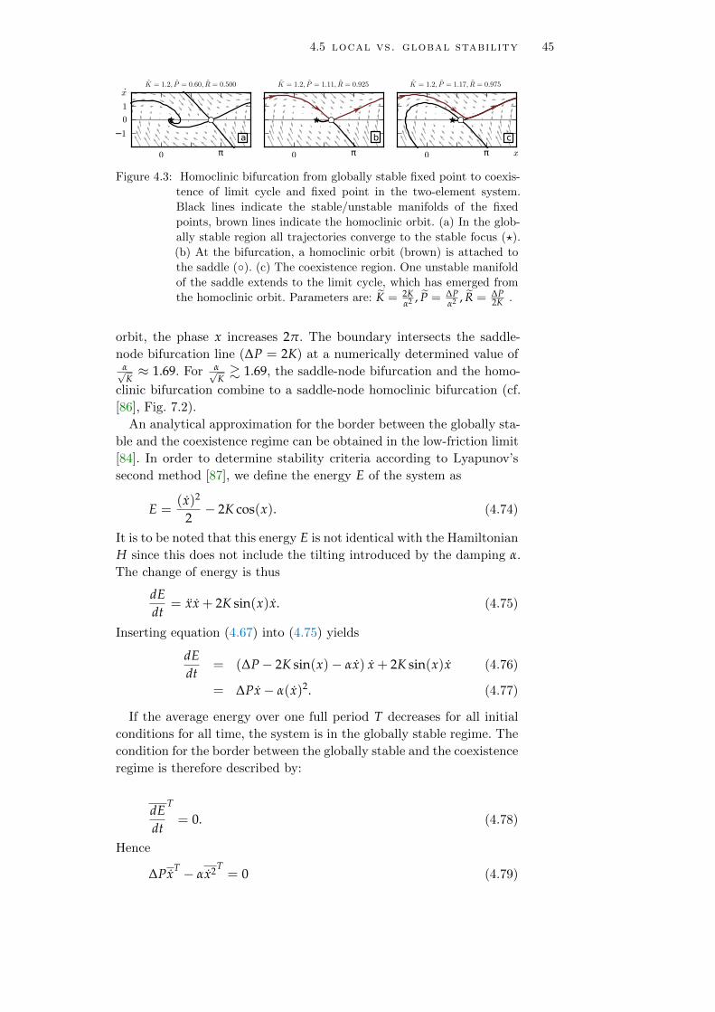
4.5 local vs. global stability 45
0 π
−1
0
1
x
a
0 π
b
0 π x
c
Figure 4.3: Homoclinic bifurcation from globally stable fixed point to coexis-
tence of limit cycle and fixed point in the two-element system.
Black lines indicate the stable/unstable manifolds of the fixed
points, brown lines indicate the homoclinic orbit. (a) In the glob-
ally stable region all trajectories converge to the stable focus (?).
(b) At the bifurcation, a homoclinic orbit (brown) is attached to
the saddle (). (c) The coexistence region. One unstable manifold
of the saddle extends to the limit cycle, which has emerged from
the homoclinic orbit. Parameters are: K = 2Kα2 , P = ∆P
α2 , R = ∆P2K .
orbit, the phase x increases 2π. The boundary intersects the saddle-
node bifurcation line (∆P = 2K) at a numerically determined value ofα√K≈ 1.69. For α√
K& 1.69, the saddle-node bifurcation and the homo-
clinic bifurcation combine to a saddle-node homoclinic bifurcation (cf.
[86], Fig. 7.2).
An analytical approximation for the border between the globally sta-
ble and the coexistence regime can be obtained in the low-friction limit
[84]. In order to determine stability criteria according to Lyapunov’s
second method [87], we define the energy E of the system as
E =(x)2
2− 2K cos(x). (4.74)
It is to be noted that this energy E is not identical with the Hamiltonian
H since this does not include the tilting introduced by the damping α.
The change of energy is thus
dEdt
= xx + 2K sin(x)x. (4.75)
Inserting equation (4.67) into (4.75) yields
dEdt
= (∆P− 2K sin(x)− αx) x + 2K sin(x)x (4.76)
= ∆Px− α(x)2. (4.77)
If the average energy over one full period T decreases for all initial
conditions for all time, the system is in the globally stable regime. The
condition for the border between the globally stable and the coexistence
regime is therefore described by:
dEdt
T
= 0. (4.78)
Hence
∆PxT − αx2T= 0 (4.79)

46 article – supply networks: instabilities without overload
is the condition for the border between the globally stable and the
coexistence regime.
We can now calculate
xT=
1T
∫ T
0xdt =
1T
∫ π
−πdx =
2π
T(4.80)
and
x2T=
1T
∫ T
0x2dt =
1T
∫ π
−πxdx (4.81)
=1T
∫ π
−π
√2E(x, x) + 4K cos(x)dx. (4.82)
Inserting equation (4.79), we get
∆P2π
T=
α
T
∫ π
−π
√2E(x, x) + 4K cos(x)dx. (4.83)
At the parameters where a globally stable fixed point loses global
stability, there will exist a trajectory of x which will satisfy x = 0 at
each successive peak of the potential landscape (cf. Fig. 4.1). Therefore
we have Epeak = 2K. At the low friction approximation, we can neglect
energy dissipation and hence assume E to be constant throughout the
period. So we substitute E(x, x) = 2K in (4.83):∫ π
−π
√4K + 4K cos(x)dx = 8
√2K. (4.84)
We thus find for the low-friction approximation the following border
between the globally stable and the coexistence regime (cf. (4.83))
∆P =4√
2π· α√
K. (4.85)
The excellent agreement of the low-friction approximation (red line)
for α/√
K < 0.6 with the numerically calculated border (blue curve)
separating the two regimes is illustrated in Fig. 4.2.
4.6 instabilities with and without overload
The regular operation of a power grid is described by a stable fixed point
of the oscillator model (4.20). When a parameter, such as the power Pjor the transmission capacity Kjk, is varied smoothly, in some cases this
fixed point can be lost, which signals an eventual desynchonization of
the grid. If the local frequency deviates from the reference Ω by more
than a fixed security margin (typically 200 mHz, cf. [88]), an emergency
shutdown is carried out which can lead to a large-scale power outage
(see, e.g., [89, 56, 57]). In this section we discuss the physical aspects
of this instability.

4.6 instabilities with and without overload 47
We first note that a stable fixed point can be lost only via a saddle-
node bifurcation as described by Lemma 4.3.3. The fixed point is stable
iff the real part of all eigenvalues of the Jacobian is smaller than or equal
to zero. The bifurcation thus occurs when
<(λ`±)→ 0 ⇔ µ` → 0. (4.86)
for any ` ∈ 2, . . . , N. We recall that µ1 = 0, which corresponds to a
global shift of the phases θj, has no physical significance.
Interestingly, the loss of a stable fixed point is generally not equiva-
lent to an overload of one or more transmission lines. In particular, we
can distinguish two different scenarios.
4.6.1 In normal operation, instability implies overload
When a power grid is only weakly loaded, the phase differences along
each edge remain small. The power flow over the transmission line (j, k)
increases monotonically with the phase difference as long as |θj− θk| ≤π/2 (cf. equation (4.15)). If this condition holds for all edges in the
network, the grid is dynamically stable, as proved in Corollary 4.6.1
below, and we can find a direct graph theoretic interpretation of any
bifurcation. We call this normal operation.
Corollary 4.6.1. A fixed point is stable if |θ∗i − θ∗j | ≤ π/2 holds for
all edges (i, j) of the network.
Proof. We define the residual capacity of each transmission line as
Kredij = Kij cos(θj − θi). (4.87)
If |θ∗i − θ∗j | ≤ π/2 holds for all edges, then ∀i, j ∈ ZN
0 ≥ Kij cos(θ∗i − θ∗j ) (4.88)
= Kij
√1− sin2(θj − θi)
=√
K2ij − F2
ij (4.89)
where Fij = Kij sin (θj − θi) is the power flow from node j to node i. Let
us define a meta-graph G with the same set of vertices and edges as
the original power grid, but with edge weights wij = Kredij . The Hesse
matrix M as defined in (4.48) then becomes the Laplacian matrix of
the meta-graph (details in Appendix 4.A). It is a well known result [52]
that the eigenvalues of the Laplacian of a graph with non-negative edge
weights satisfy:
0 = µ1 ≤ µ2 ≤ · · · ≤ µN . (4.90)
Stability of the fixed point directly follows from theorem 4.3.1.
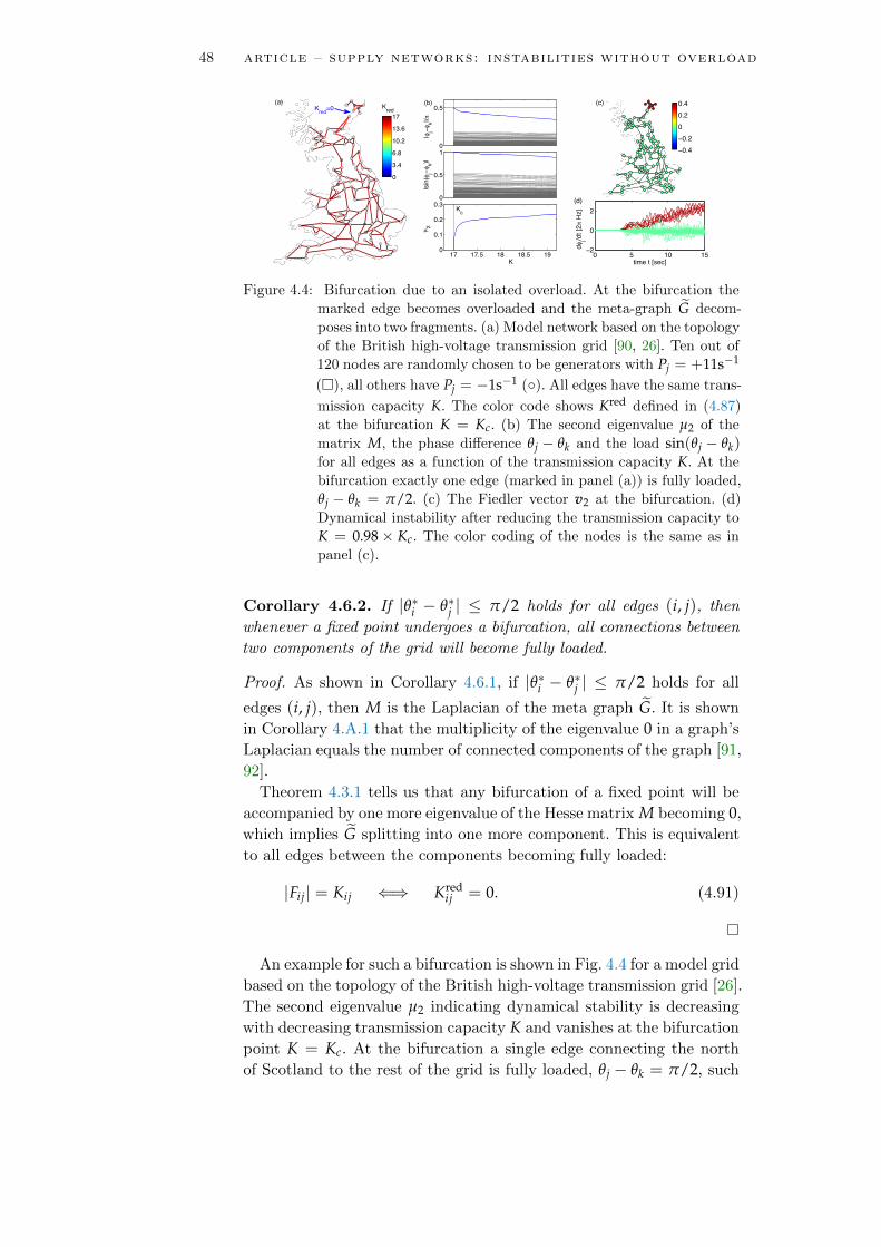
48 article – supply networks: instabilities without overload
Kred=0
(a) Kred
0
3.4
6.8
10.2
13.6
17
0
0.5
|!j−! k|/"
(b)
0
0.5
1
|sin(!j−! k)|
17 17.5 18 18.5 190
0.1
0.2
0.3
K
µ2
Kc
(c)
−0.4−0.20 0.2 0.4
0 5 10 15−2
0
2
time t [sec]
d!j/d
t [2"
Hz]
(d)
Figure 4.4: Bifurcation due to an isolated overload. At the bifurcation the
marked edge becomes overloaded and the meta-graph G decom-
poses into two fragments. (a) Model network based on the topology
of the British high-voltage transmission grid [90, 26]. Ten out of
120 nodes are randomly chosen to be generators with Pj = +11s−1
(), all others have Pj = −1s−1 (). All edges have the same trans-
mission capacity K. The color code shows Kred defined in (4.87)
at the bifurcation K = Kc. (b) The second eigenvalue µ2 of the
matrix M, the phase difference θj − θk and the load sin(θj − θk)for all edges as a function of the transmission capacity K. At the
bifurcation exactly one edge (marked in panel (a)) is fully loaded,
θj − θk = π/2. (c) The Fiedler vector v2 at the bifurcation. (d)
Dynamical instability after reducing the transmission capacity to
K = 0.98× Kc. The color coding of the nodes is the same as in
panel (c).
Corollary 4.6.2. If |θ∗i − θ∗j | ≤ π/2 holds for all edges (i, j), then
whenever a fixed point undergoes a bifurcation, all connections between
two components of the grid will become fully loaded.
Proof. As shown in Corollary 4.6.1, if |θ∗i − θ∗j | ≤ π/2 holds for all
edges (i, j), then M is the Laplacian of the meta graph G. It is shown
in Corollary 4.A.1 that the multiplicity of the eigenvalue 0 in a graph’s
Laplacian equals the number of connected components of the graph [91,
92].
Theorem 4.3.1 tells us that any bifurcation of a fixed point will be
accompanied by one more eigenvalue of the Hesse matrix M becoming 0,
which implies G splitting into one more component. This is equivalent
to all edges between the components becoming fully loaded:
|Fij| = Kij ⇐⇒ Kredij = 0. (4.91)
An example for such a bifurcation is shown in Fig. 4.4 for a model grid
based on the topology of the British high-voltage transmission grid [26].
The second eigenvalue µ2 indicating dynamical stability is decreasing
with decreasing transmission capacity K and vanishes at the bifurcation
point K = Kc. At the bifurcation a single edge connecting the north
of Scotland to the rest of the grid is fully loaded, θj − θk = π/2, such
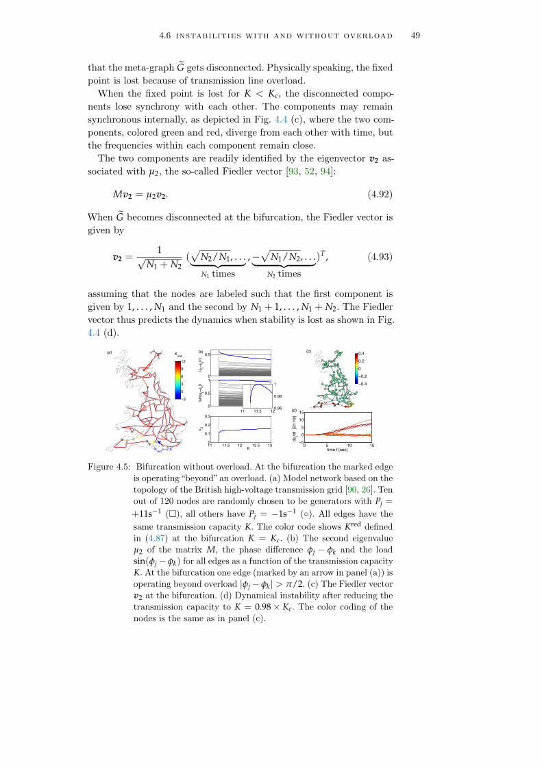
4.6 instabilities with and without overload 49
that the meta-graph G gets disconnected. Physically speaking, the fixed
point is lost because of transmission line overload.
When the fixed point is lost for K < Kc, the disconnected compo-
nents lose synchrony with each other. The components may remain
synchronous internally, as depicted in Fig. 4.4 (c), where the two com-
ponents, colored green and red, diverge from each other with time, but
the frequencies within each component remain close.
The two components are readily identified by the eigenvector v2 as-
sociated with µ2, the so-called Fiedler vector [93, 52, 94]:
Mv2 = µ2v2. (4.92)
When G becomes disconnected at the bifurcation, the Fiedler vector is
given by
v2 =1√
N1 + N2(√
N2/N1, . . .︸ ︷︷ ︸N1 times
,−√
N1/N2, . . .︸ ︷︷ ︸N2 times
)T, (4.93)
assuming that the nodes are labeled such that the first component is
given by 1, . . . , N1 and the second by N1 + 1, . . . , N1 + N2. The Fiedler
vector thus predicts the dynamics when stability is lost as shown in Fig.
4.4 (d).
(a) Kred
Kred=−2.8
−3
0
3
6
9
12
0
0.5
|!j−! k|/"
(b)
0
0.5
1
|sin
(!j−! k)|
11 11.5 12 12.5 13 0
0.1
0.2
0.3
K
µ2
11 11.5 120.96
0.98
1
(c)
−0.4
−0.2
0
0.2
0.4
0 5 10 15−5
05
1015
time t [sec]
d!j/d
t [2"
Hz]
(d)
Figure 4.5: Bifurcation without overload. At the bifurcation the marked edge
is operating“beyond”an overload. (a) Model network based on the
topology of the British high-voltage transmission grid [90, 26]. Ten
out of 120 nodes are randomly chosen to be generators with Pj =
+11s−1 (), all others have Pj = −1s−1 (). All edges have the
same transmission capacity K. The color code shows Kred defined
in (4.87) at the bifurcation K = Kc. (b) The second eigenvalue
µ2 of the matrix M, the phase difference φj − φk and the load
sin(φj− φk) for all edges as a function of the transmission capacity
K. At the bifurcation one edge (marked by an arrow in panel (a)) is
operating beyond overload |φj− φk| > π/2. (c) The Fiedler vector
v2 at the bifurcation. (d) Dynamical instability after reducing the
transmission capacity to K = 0.98× Kc. The color coding of the
nodes is the same as in panel (c).

50 article – supply networks: instabilities without overload
4.6.2 Instability without overload
A different scenario can occur when the condition |θ∗i − θ∗j | ≤ π/2 is
not satisfied for one or more edges. This is possible for a stable fixed
point in complex networks at the edge of the stable parameter region.
Then we can have Kredjk < 0 such that the meta-graph is no longer a
non-negative graph and the results discussed in the previous section do
not apply.
In this case the bifurcation of a fixed point is generally not asso-
ciated with any overload. In particular, the grid is already operating
‘beyond’ an overload at the bifurcation point. An example of such a
bifurcation is shown in Fig. 4.5. The marked edge has a phase differ-
ence of |θ∗j − θ∗k | > π/2 such that Kredjk < 0. The loss of stability is a
collective effect of the entire grid and in particular there is no simple
graph theoretical interpretation of the bifurcation. Consequently, the
Fiedler vector defined in (4.92) only gives a limited insight into the
desynchronization dynamics when the fixed point is lost.
4.6.3 Relevance of bifurcation scenarios
The two bifurcation scenarios regularly occur in networks with complex
topologies. We have analyzed the bifurcation for 200 realizations of the
model network based on the topology of the British power grid with
random generator positions (see Fig. 4.6). We find that the loss of the
steady state is caused by an isolated overload in approximately 40% of
the sample networks while the grid is operating beyond overload in the
remaining 60% of all cases.
We note that the loss of a steady state and the following desynchro-
nization generally leads to a large-scale power outage (cf. [89, 56, 57]).
In current power grids this can happen only in periods of extreme loads
while the phase difference is generally much smaller than π/2 in periods
of average load. However, extreme loads are expected to become much
more likely in the future if the power grid is not sufficiently adapted to
the energy transition to renewable sources [64].
The two examples shown in Fig. 4.4 and Fig. 4.5 capture the essential
mathematical aspects of this bifurcation for two model networks. Hence
they are of interest both for fundamental research and as a guideline
for the the analysis of real-world power grids though being simplified.
In the figures we have illustrated the system stability for two model
networks as a function of the parameter K in the very tradition of
the physics literature on oscillator models (cf. [1, 4, 2] and references
therein). In real world grids, the connectivity Kij is generally fixed while
generation and load can change strongly. As an essential parameter
affecting stability is the transported power P relative to the connectivity
Kij, we vary Kij to study qualitative changes in the collective dynamics
of the network.
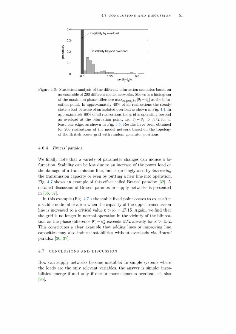
4.7 conclusions and discussion 51
0.5 0.55 0.60
0.1
0.2
0.3
0.4
max |θj−θ
k|/π
prob
abili
ty
instability by overload
instability beyond overload
Figure 4.6: Statistical analysis of the different bifurcation scenarios based on
an ensemble of 200 different model networks. Shown is a histogram
of the maximum phase difference maxedges(j,k) |θj− θk| at the bifur-
cation point. In approximately 40% of all realizations the steady
state is lost because of an isolated overload as shown in Fig. 4.4. In
approximately 60% of all realizations the grid is operating beyond
an overload at the bifurcation point, i.e. |θj − θk| > π/2 for at
least one edge, as shown in Fig. 4.5. Results have been obtained
for 200 realizations of the model network based on the topology
of the British power grid with random generator positions.
4.6.4 Braess’ paradox
We finally note that a variety of parameter changes can induce a bi-
furcation. Stability can be lost due to an increase of the power load or
the damage of a transmission line, but surprisingly also by increasing
the transmission capacity or even by putting a new line into operation.
Fig. 4.7 shows an example of this effect called Braess’ paradox [32]. A
detailed discussion of Braess’ paradox in supply networks is presented
in [36, 37].
In this example (Fig. 4.7 ) the stable fixed point ceases to exist after
a saddle node bifurcation when the capacity of the upper transmission
line is increased to a critical value κ > κc = 17.15. Again, we find that
the grid is no longer in normal operation in the vicinity of the bifurca-
tion as the phase difference θ∗5 − θ∗4 exceeds π/2 already for κ > 15.2.
This constitutes a clear example that adding lines or improving line
capacities may also induce instabilities without overloads via Braess’
paradox [36, 37].
4.7 conclusions and discussion
How can supply networks become unstable? In simple systems where
the loads are the only relevant variables, the answer is simple: insta-
bilities emerge if and only if one or more elements overload, cf. also
[95].

52 article – supply networks: instabilities without overload
As we intended, we have demonstrated in this article how instability
can also emerge in the absence of any overloads. We have explicated
stability conditions for fixed points (steady operation) of oscillatory
power grid models [19, 26, 71], where in addition to the pure flows,
phase variables play a crucial role. We linked a Hamiltonian descrip-
tion to existence and bifurcation types of fixed points. In particular, we
demonstrated that instabilities may emerge with and without transmis-
sion line overloads and that – through Braess’ paradox [36, 37] – adding
new lines may also create collective instabilities without line overloads.
0 5 10 15 20
−0.5
0
0.5
κ
phase
differen
ces
(θj−
θj−
1)/π
(b)
0 5 10 15 20
0
100
200
eigen
values
µ
κ
(c)
15 16 17 18κ
0.4
0.5
0.6
κc
Figure 4.7: Loss of stability due to the increase of local transmission capacity
in a circular network. A stable (—) and an unstable (−−−) fixed
point vanish in a saddle-node bifurcation at the critical point κc =17.15. The stable fixed point (blue) is lost. (a) Topology of the
network. The capacity of the upper edge (3, 4) is increased by
an amount κ. (b) Phase differences along the edges of the cycle.
Close to the bifurcation, the phase difference |θ5− θ4| exceeds π/2for the stable fixed point (see inset). (c) Eigenvalues of the Hesse
matrix M, which yield the eigenvalues of the Jacobian via (4.62).
Parameters are K = 50 and P0 = 49.
Like the coupled phase oscillator model described here in the context
of power grids, the function of many physical and biological supply net-
works depends on and involves quantities other than the network load.
A notable example from biology is leaf vasculature and stomatal patch-
iness. Stomatal patchiness is the oscillatory dynamics of the opening
and closing of patches of leaf stomata, which is believed to be the result
of hydraulic and elastic coupling between neighbouring stomata. This
dynamics can arise in a self organised manner in situations where a uni-
form stomatal aperture should be expected. Although recent progress
has been made, stomatal patchiness is still not completely understood
[96], especially in the context of the underlying hydraulic coupling of
the stomata to the vascular system.

4.7 conclusions and discussion 53
Similarly, the plant phloem is a dynamical transport system involving
a number of interdependent quantities. The phloem vascular elements
transfer sap (a sugar rich water solution) from and between the photo-
synthesising tissues to the rest of the plant. Sugars are being loaded in
the phloem actively or passively at the sites of photosynthesis and the
rate of sugar production and loading (determining the vascular network
operation) can vary from site to site. The sugar concentration is a field
of independent variables coupled to the network load (phloem fluid
flow), and depending on the loading regime, the system has a potential
of a rich dynamical behaviour [97, 98]. The plant phloem might thus
constitute a biological candidate system where instabilities of normal
supply function may emerge without overloads.
acknowledgement
We acknowledge support from the Bundesministerium fur Bildung und
Forschung and by a grant of the Max Planck Society to M.T.

A P P E N D I X
4.a properties of graph laplacian
Definition 4.A.1. Let G be a weighted graph with n nodes with all the
edge weights wij ≥ 0. The Laplacian M is an N × N matrix given by:
Mij = −wij + δij
N
∑k=1
wik (4.94)
Theorem 4.A.1. In a fully connected graph G, the Laplacian L has
exactly one zero eigenvalue.
Proof. The Laplacian M obviously has one zero eigenvalue: the corre-
sponding eigenvector being v0 = (1, 1, · · · , 1):
(Mv0)i = ∑j
Mijv0j
= ∑j
Mij
= ∑j
[∑
kδijwik − wij
]= 0
(4.95)
Suppose there is another eigenvector v′ with eigenvalue 0. Then:
0 = v′T Mv′
= ∑ij
v′i Mijv′j
= ∑ij
v′i
(∑
kδijwik − wij
)v′j
= ∑j
(∑
kwjk
)v′2j −∑
ijwijv′iv
′j
= ∑i<j
[√wij
(v′i − v′j
)]2
(4.96)
Therefore it follows that√wij(v′i − v′j) = 0 for all i, j ∈ ZN. This
implies whenever two nodes are connected by an edge (wij 6= 0), vi = vj.
Now, by virtue of G being connected, v′i = v′j must hold for all (i, j).But that implies v′ = v0, up to a multiplicative constant.
Corollary 4.A.1. The multiplicity of 0 eigenvalue in the Laplacian of
a graph equals its number of connected components.
56 article – supply networks: instabilities without overload
Proof. For a graph with c connected components, if the node indices
are chosen properly, the Laplacian L will be in a block diagonal form
with c blocks. Then following the same reasoning as in Theorem 4.A.1,
the result follows.
references
[1] Y. Kuramoto. “Self-entrainment of a population of coupled non-
linear oscillators.” In: International Symposium on on Mathe-
matical Problems in Theoretical Physics. Ed. by H. Araki. Lec-
ture Notes in Physics Vol. 39. New York: Springer, 1975, p. 420.
[2] Juan A Acebron et al.“The Kuramoto model: A simple paradigm
for synchronization phenomena.” In: Reviews of modern physics
77.1 (2005), p. 137.
[4] Steven H. Strogatz.“From Kuramoto to Crawford: Exploring the
onset of synchronization in populations of coupled oscillators.”
In: Physica D: Nonlinear Phenomena 143 (2000), p. 1.
[19] Giovanni Filatrella, Arne Hejde Nielsen, and Niels Falsig Ped-
ersen. “Analysis of a power grid using a Kuramoto-like model.”
In: The European Physical Journal B - Condensed Matter and
Complex Systems 61.4 (2008), pp. 485–491.
[26] Martin Rohden et al. “Self-organized synchronization in decen-
tralized power grids.” In: Physical review letters 109.6 (2012),
p. 064101.
[32] Dietrich Braess. “Uber ein Paradoxon aus der Verkehrsplanung.”
In: Unternehmensforschung 12.1 (1968), pp. 258–268.
[36] Dirk Witthaut and Marc Timme. “Braess’s paradox in oscillator
networks, desynchronization and power outage.”In: New journal
of physics 14.8 (2012), p. 083036.
[37] Dirk Witthaut and Marc Timme. “Nonlocal failures in complex
supply networks by single link additions.” In: The European
Physical Journal B 86.9 (2013), p. 377.
[49] Florian Dorfler, Michael Chertkov, and Francesco Bullo. “Syn-
chronization in complex oscillator networks and smart grids.” In:
Proceedings of the National Academy of Sciences 110.6 (2013),
pp. 2005–2010.
[52] M. E. J. Newman. Networks – An introduction. Oxford: Oxford
University Press, 2010. isbn: 978-0-19-920665-0.
[56] U.S.-Canada Power System Outage Task Force. https://reports.
energy.gov/BlackoutFinal-Web.pdf. 2004.
References 57
[57] Union for the Coordination of Transmission of Electricity. Final
report on the system disturbance on 4 November 2006. http://
www.entsoe.eu/~library/publications/ce/otherreports/
Final-Report-20070130.pdf. 2007.
[62] Emma Marris. “Energy: Upgrading the grid.” In: Nature News
454.7204 (2008), pp. 570–573.
[63] John A Turner. “A realizable renewable energy future.” In: Sci-
ence 285.5428 (1999), pp. 687–689.
[64] Thiemo Pesch, H-J Allelein, and J-F Hake.“Impacts of the trans-
formation of the German energy system on the transmission
grid.” In: The European Physical Journal Special Topics 223.12
(2014), pp. 2561–2575.
[65] Dominik Heide et al. “Seasonal optimal mix of wind and solar
power in a future, highly renewable Europe.” In: Renewable En-
ergy 35.11 (2010), pp. 2483–2489.
[66] Frank Bottcher, Joachim Peinke, et al. “Small and large scale
fluctuations in atmospheric wind speeds.” In: Stochastic envi-
ronmental research and risk assessment 21.3 (2007), pp. 299–
308.
[67] Patrick Milan, Matthias Wachter, and Joachim Peinke. “Turbu-
lent character of wind energy.” In: Physical review letters 110.13
(2013), p. 138701.
[68] Arthur R Bergen and David J Hill. “A structure preserving
model for power system stability analysis.” In: IEEE Transac-
tions on Power Apparatus and Systems 1 (1981), pp. 25–35.
[69] David J Hill and Guanrong Chen. “Power systems as dynamic
networks.” In: Circuits and Systems, 2006. ISCAS 2006. Pro-
ceedings. 2006 IEEE International Symposium on. IEEE. 2006,
4–pp.
[70] Jan Machowski, Janusz W Bialek, and James Richard Bumby.
Power system dynamics, stability and control. New York: John
Wiley & Sons, 2008.
[71] Martin Rohden et al. “Impact of network topology on synchrony
of oscillatory power grids.” In: Chaos: An Interdisciplinary Jour-
nal of Nonlinear Science 24.1 (2014), p. 013123.
[72] Adilson E Motter et al. “Spontaneous synchrony in power-grid
networks.” In: Nature Physics 9.3 (2013), pp. 191–197.
[73] Peter J Menck et al. “How dead ends undermine power grid
stability.” In: Nature communications 5 (2014).
[74] Prabha Kundur, Neal J Balu, and Mark G Lauby. Power system
stability and control. Vol. 7. McGraw-hill New York, 1994.

58 article – supply networks: instabilities without overload
[75] Yoshihiko Susuki, Igor Mezic, and Takashi Hikihara. “Global
swing instability of multimachine power systems.” In: Decision
and Control, 2008. CDC 2008. 47th IEEE Conference on. IEEE.
2008, pp. 2487–2492.
[76] Yoshihiko Susuki, Igor Mezic, and Takashi Hikihara. “Coherent
swing instability of power grids.”In: Journal of nonlinear science
21.3 (2011), pp. 403–439.
[77] Florian Dorfler and Francesco Bullo. “Kron reduction of graphs
with applications to electrical networks.” In: IEEE Transactions
on Circuits and Systems I: Regular Papers 60.1 (2013), pp. 150–
163.
[78] Katrin Schmietendorf et al. “Self-organized synchronization and
voltage stability in networks of synchronous machines.” In: The
European Physical Journal Special Topics 223.12 (2014), pp. 2577–
2592.
[79] Hsiao-Dong Chiang, Felix Wu, and P Varaiya. “Foundations of
direct methods for power system transient stability analysis.”
In: IEEE Transactions on Circuits and systems 34.2 (1987),
pp. 160–173.
[80] CJ Perez and F Ritort. “A moment-based approach to the dy-
namical solution of the Kuramoto model.” In: Journal of Physics
A: Mathematical and General 30.23 (1997), p. 8095.
[81] James Howard. “Stability of Hamiltonian equilibria.” In: Schol-
arpedia 8 (2013), p. 3627. doi: 10.4249/scholarpedia.3627.
[82] Hassan K Khalil and JW Grizzle. Nonlinear systems. Vol. 3.
Prentice hall Upper Saddle River, 2002.
[83] M Levi, Frank C Hoppensteadt, and WL Miranker. “Dynamics
of the Josephson junction.” In: Quarterly of Applied Mathemat-
ics 36.2 (1978), pp. 167–198.
[84] Hannes Risken. Fokker-planck equation. Springer, 1996, pp. 63–
95.
[85] Peter J Menck et al.“How basin stability complements the linear-
stability paradigm.” In: Nature Physics 9.2 (2013), pp. 89–92.
[86] Yuri A Kuznetsov. Elements of applied bifurcation theory. Vol. 112.
Springer Science & Business Media, 2013.
[87] Patrick C Parks. “AM Lyapunov’s stability theory - 100 years
on.” In: IMA journal of Mathematical Control and Information
9.4 (1992), pp. 275–303.
[88] Union for the Coordination of Transmission of Electricity. Con-
tinental Europe Operation Handbook. https://www.entsoe.
eu/publications/system-operations-reports/operation-
handbook/Pages/default.aspx. 2014.
References 59
[89] Peter Fairley. “The unruly power grid.” In: IEEE Spectrum 41.8
(2004), pp. 22–27.
[90] Ingve Simonsen et al. “Transient dynamics increasing network
vulnerability to cascading failures.” In: Physical review letters
100.21 (2008), p. 218701.
[91] William N Anderson Jr and Thomas D Morley. “Eigenvalues of
the Laplacian of a graph.” In: Linear and multilinear algebra
18.2 (1985), pp. 141–145.
[92] Bojan Mohar et al. “The Laplacian spectrum of graphs.” In:
Graph theory, combinatorics, and applications 2.871-898 (1991),
p. 12.
[93] Miroslav Fiedler.“Algebraic connectivity of graphs.”In: Czechoslo-
vak mathematical journal 23.2 (1973), pp. 298–305.
[94] Santo Fortunato. “Community detection in graphs.” In: Physics
reports 486.3 (2010), pp. 75–174.
[95] Surya D Pathak et al. “Complexity and adaptivity in supply net-
works: Building supply network theory using a complex adaptive
systems perspective.” In: Decision sciences 38.4 (2007), pp. 547–
580.
[96] Antonio MT Ramos and Carmen PC Prado. “Role of hystere-
sis in stomatal aperture dynamics.” In: Physical Review E 87.1
(2013), p. 012719.
[97] Kare Hartvig Jensen et al. “Optimality of the Munch mechanism
for translocation of sugars in plants.” In: Journal of the Royal
Society Interface 8.61 (2011), pp. 1155–1165.
[98] JW Patrick. “Phloem unloading: sieve element unloading and
post-sieve element transport.” In: Annual review of plant biology
48.1 (1997), pp. 191–222.

5A RT I C L E – C Y C L E F L OW S A N D M U LT I S TA B I L I T Y
I N O S C I L L AT O R N E T WO R K S
Debsankha Manik1, Marc Timme1,2,3, Dirk Witthaut4,5
1 Network Dynamics, Max Planck Institute for Dynamics and Self-
Organization (MPI DS), D-37077 Gottingen, Germany
2 Chair for Network Dynamics, Institute for Theoretical Physics
and Center for Advancing Electronics Dresden (cfaed), Technical
University of Dresden, 01069 Dresden, Germany
3 Department of Physics, Technical University Darmstadt, 64289
Darmstadt, Germany
4 Forschungszentrum Julich, Institute for Energy and Climate Re-
search – Systems Analysis and Technology Evaluation (IEK-STE),
52425 Julich, Germany
5 Institute for Theoretical Physics, University of Cologne, 50937
Koln, Germany
Published in:
Chaos: An Interdisciplinary Journal of Nonlinear Science 27 (8)
2017: 083123
DOI (for Published version):
10.1063/1.4994177
Legal note:
This is an open-access publication licensed under the Creative
Commons Attribution 4.0 International License. To view a copy
of this license, visit http://creativecommons.org/licenses/
by/4.0/. The final publication is available at http://aip.scitation.
org/doi/10.1063/1.4994177.
Original contribution:
I carried out most of the analytical calculations behind the results. I
performed the numerical computations for Sec V, and contributed all
results for Sec II, III, V.C–V.F. I wrote most of the text sections, in-
cluding Discussion and Conclusion. I revised manuscript during revision
process, updating texts and figures as per referee reports.

Cycle flows and multistability in oscillatory networks
Debsankha Manik,1 Marc Timme,1,2,3 and Dirk Witthaut4,5
1Network Dynamics, Max Planck Institute for Dynamics and Self-Organization (MPIDS), 37077 G€ottingen,Germany2Chair for Network Dynamics, Institute for Theoretical Physics and Center for Advancing Electronics Dresden(cfaed), Technical University of Dresden, 01069 Dresden, Germany3Department of Physics, Technical University Darmstadt, 64289 Darmstadt, Germany4Forschungszentrum J€ulich, Institute for Energy and Climate Research - Systems Analysis and TechnologyEvaluation (IEK-STE), 52425 J€ulich, Germany5Institute for Theoretical Physics, University of Cologne, 50937 K€oln, Germany
(Received 3 January 2017; accepted 3 July 2017; published online 29 August 2017)
We study multistability in phase locked states in networks of phase oscillators under both
Kuramoto dynamics and swing equation dynamics—a popular model for studying coarse-scale
dynamics of an electrical AC power grid. We first establish the existence of geometrically frus-
trated states in such systems—where although a steady state flow pattern exists, no fixed point
exists in the dynamical variables of phases due to geometrical constraints. We then describe the sta-
ble fixed points of the system with phase differences along each edge not exceeding p=2 in terms
of cycle flows—constant flows along each simple cycle—as opposed to phase angles or flows. The
cycle flow formalism allows us to compute tight upper and lower bounds to the number of fixed
points in ring networks. We show that long elementary cycles, strong edge weights, and spatially
homogeneous distribution of natural frequencies (for the Kuramoto model) or power injections (for
the oscillator model for power grids) cause such networks to have more fixed points. We generalize
some of these bounds to arbitrary planar topologies and derive scaling relations in the limit of large
capacity and large cycle lengths, which we show to be quite accurate by numerical computation.
Finally, we present an algorithm to compute all phase locked states—both stable and unstable—for pla-
nar networks. VC 2017 Author(s). All article content, except where otherwise noted, is licensed undera Creative Commons Attribution (CC BY) license (http://creativecommons.org/licenses/by/4.0/).[http://dx.doi.org/10.1063/1.4994177]
The functions of many networked systems in physics, biol-
ogy, or engineering rely on a coordinated or synchronized
dynamics of their constituents. In power grids for example,
all generators must run at the same frequency and their
phases need to lock to guarantee a steady power flow.
Here, we analyze the existence and multitude of states
exhibiting this phase locking behaviour. Focusing on edge
and cycle flows instead of the nodal phases, we derive rigor-
ous results on the existence and number of such states.
Generally, multiple phase-locked states coexist in networks
with edges capable of carrying high flows, long elementary
cycles, and a homogeneous spatial distribution of natural
frequencies or power injections. Utilizing concepts from
the graph theory, we derive scaling relations for the num-
ber of such states in plane embedded networks. We also
offer an algorithm to systematically compute all phase-
locked states, both stable and unstable.
I. FROM KURAMOTO OSCILLATORS TO POWERGRIDS
Coupled oscillator models are ubiquitous in science and
technology, describing the collective dynamics of various
systems on micro- to macro-scale. Research on coupled
oscillators dates back to Christian Huygens, who noticed that
two clocks synchronize when they are coupled.1 One of the
most important mathematical models was introduced by
Kuramoto2,3 and successfully applied to describe the collec-
tive dynamics of coupled Josephson junctions,4 neuronal net-
works,5 chemical oscillators,6 and a variety of other
synchronization phenomena.7–10
That model3 describes the dynamics of N coupled limit
cycle oscillators. The equations of motions for the phases
hj; j 2 f1;…;Ng are given by
d
dthj ¼ xj þ
XN
‘¼1
Kj;‘ sin h‘ hj
: (1)
The coupling matrix is assumed to be symmetric, Kj;‘ ¼ K‘;j,
and xj are the natural frequencies of the oscillators.
Throughout this article, we consider systems where all
Kj;‘ 0, i.e., the units attract each other and do not repel.
A similar model of second-order oscillators describes
the collective phenomena of animal flocks11,12 or human
crowds13 as well as the coarse-scale dynamics of power
grids.14–20
For power grids, for instance, the units j describe syn-
chronous machines, generators, or motors, whose state is
completely described by their phase hj and the phase velocity_hj relative to the reference frequency of the grid, typically
rotating at 50 Hz or 60 Hz. The acceleration (deceleration) of
the machines is proportional to the sum of the mechanical
power Pj generated (consumed) by the machine including
1054-1500/2017/27(8)/083123/19 VC Author(s) 2017.27, 083123-1
CHAOS 27, 083123 (2017)
62 article – cycle flows and multistability in oscillator networks

damping and electric power exchanged with the grid. The
detailed equations of motion are given by
Mjd2
dt2hj þ Dj
d
dthj ¼ Pj þ
X‘¼1
Kj;‘ sin h‘ hj
; (2)
where Mj is an inertia term and Dj a damping constant. The
coupling constants Kj;‘ ¼ U2Bj;‘ are determined by the volt-
age U of the grid, which is assumed to be constant, and the
admittance Bj;‘ of the electrical transmission line joining
node j and node ‘. The flow of electric real power from node
‘ to node j is
Fj;‘ ¼ Kj;‘ sinðh‘ hjÞ ¼ Kj;‘Sj;‘: (3)
It is useful to describe the interaction topology of the system
as a weighted graph G(V, E), whose vertex set V is identical
to the set of oscillators and edge set E is given by the set of
all inter-oscillator coupling pairs, i.e., all pairs with K‘;j > 0.
We use the term network21 (rather than the term graph) for
the entire system with given natural frequencies xj or the
powers Pj.
Here, we distinguish two types of synchronization in
oscillator networks. Traditionally, the emergence of partial
synchrony has received the most interest of the physics com-
munity.2,3,7,8 In his seminal work, Kuramoto investigated a
set of oscillators with global coupling, Kj;‘ ¼ K=N, and natu-
ral frequencies drawn at random from a unimodal symmetric
distribution gðxÞ. If the coupling constant K exceeds a criti-
cal value Kc, a fraction of the oscillators start to synchronize
in the sense that they rotate at the same angular velocity
although their natural frequencies differ. In this state of par-tial frequency locking, commonly referred to in the
Kuramoto oscillator literature as “partial synchrony,”8 the
phases of parts of the oscillators are ordered, but they are not
strictly phase-locked, such that the phase difference of two
synchronized oscillators ðhj h‘Þ is generally small but not
constant.
In this article, we analyze the properties of globallyphase-locked states, where all oscillators synchronize and
the phase differences ðhj h‘Þ are constant for all pairs
ðj; ‘Þ. These states are especially important for power grids,
as they describe the regular synchronous operation of the
grid.14–18 If this state is lost due to local outages or accidents,
the grid will fragment into asynchronous islands which can
no longer exchange electric energy.22 For instance, the
European power grid fragmented into three asynchronous
areas on November 4th 2006 after the shutdown of one trans-
mission line in Northern Germany. As a result, south-
western Europe suffered an under-supply on the order of
10 GW and approximately 10 million households were
disconnected.23
Without loss of generality, we takeP
jxj ¼ 0 orPjPj ¼ 0, respectively, by invoking a transformation to a
co-rotating frame of reference. The globally phase-
locked states are then the fixed points of the system. For
both the Kuramoto model and the power grid model,
these states are given by the solutions of the transcenden-
tal equations
Pj þXN
‘¼1
Kj;‘ sin ðh‘ hjÞ ¼ 0 for all j 2 f1;…;Ng; (4)
replacing Pj by xj for the Kuramoto model. In the following, we
analyze the influence of the network topology given by the cou-
pling matrix Kj;‘ on the existence of a fixed point. All results
below hold for both models; nevertheless, our intuition heavily
relies on the interpretation of Fj;‘ ¼ Kj;‘ sin ðh‘ hjÞ as a flow
which is inspired from the power grid model. The results can be
generalized to arbitrary coupling functions f instead of the sine
(see, e.g., Refs. 24 and 25). In the following, we mostly restrict
ourselves to the common sine coupling for the sake of clarity.
We note that the second order power grid model (2) evi-
dently describes a different system from the first order
Kuramoto model (1). Nevertheless, there are deep underlying
connections between these two. In the context of power
grids, in the overdamped limit, one recovers the first order
Kuramoto model. The relation of first and second order mod-
els in the context of coupled Josephson Junctions was dis-
cussed in detail in Refs. 26 and 27. Partial synchronization in
first and second order models was reviewed in Ref. 28.
II. THE NATURE AND BIFURCATIONS OF FIXEDPOINTS
Both the Kuramoto system and the oscillator model of
power grids share the same set of fixed points (4). It has been
shown that the similarity between these two systems runs
deeper, namely, the linear stability properties of those fixed
points are identical.29,30 In this section, we briefly review
some basic results on the stability of the fixed points.
We analyze the dynamical stability of a certain fixed
point h ¼ ðh1;…; hNÞ by defining the potential function
V h1; h2;…; hNð Þ ¼ X
j
Pjhj 1
2
Xi;j
Kij cos hi hj
: (5)
The fixed points correspond to the local extrema of this
potential, where @V@hj¼ 0 for all j. A fixed point h is asymptot-
ically stable if the Hesse matrix H of the potential function
HðhÞ ¼
X‘
Kred1;‘ Kred
1;2
Kred2;1
Xl
Kred2;‘
..
. ... . .
.
0BBBBBB@
1CCCCCCA (6)
with the residual capacity
Kredj;‘ ¼ Kj;‘ cosðhj h‘ Þ (7)
has positive eigenvalues only. It is worth noting that H has
one eigenvector v1 ¼ ð1; 1;…; 1Þ with eigenvalue l1 ¼ 0
because any fixed point h is arbitrary up to an additive con-
stant c. As such a global phase shift does not affect the lock-
ing of the phases, we can discard it in the following and
concentrate on the stability transversely to the solution space
fh þ cð1; 1;…; 1Þjc 2 Rg.
083123-2 Manik, Timme, and Witthaut Chaos 27, 083123 (2017)
5.2 the nature and bifurcations of fixed points 63

Lemma 1. Let the eigenvalues of H be ordered such thatl1 ¼ 0 and l2 lN. If for a given network topologyand a given fixed point,
lk > 0; for all k 2 f2; 3;…;Ng; (8)
then this fixed point is transversally asymptotically stable forboth the Kuramoto system and the power grid model system.If one of the lk < 0, then the dynamical system is linearlyunstable (this lemma and its proof have been presented inRef. 29).
Using some results from the bifurcation theory, it has
been shown in Ref. 29 that a stable fixed point can only be
lost by an inverse saddle-node bifurcation when one of the
eigenvalues becomes zero, l2 ¼ 0. At this point, linear
stability analysis is not sufficient to predict the stability of
the fixed point, but it is expected that the fixed point is
unstable.31
More insights into the loss of a fixed point when the
phase differences across all edges in the network are suffi-
ciently small can be gained:
Corollary 1. Consider a connected network. It is suffi-cient (but not necessary) for a fixed point h to be transver-sally asymptotically stable; if the condition
cosðhi hj Þ > 0 (9)
holds for all edges (i, j) in the network, then the network issaid to be in “normal operation.”
Proof. To this end, we first define a metagraph as
follows.
Definition 1 (Metagraph). Given a graph G(V, E) and aset of flows Fuv across each edge e(u, v), its metagraph ~G isan undirected graph with vertex set V and edge set E0 definedas follows. For all edges eðu; vÞ 2 E, with weight Kuv; 9, anedge eðu; vÞ 2 E0 with weight Kred
uv ¼ffiffiffiffiffiffiffiffiffiffiffiffiffiffiffiffiffiffiffiK2
uv F2uv
p, as per (7).
Then, the matrix H as defined in (6) is seen to be the
Laplacian matrix of the metagraph ~G. The eigenvalues of a
Laplacian of a connected undirected graph with positive
edge weights are always non-negative21 such that we obtain
the result.
We note that this sufficient condition for stability has
been shown in Ref. 32 using the Gershgorin circle theorem.
During normal operation, an eigenvalue of the Hesse
matrix H, as defined in (6), can become 0 only when ~Gdisconnects into two (or more) components. Such a split-
up occurs only when Kredj;‘ ¼ 0 for all the transmission
lines connecting two certain parts (denoted by G1 and G2)
of the network, meaning that these lines are completely
saturated
sinðhj h‘ Þ ¼ 61 ) jFj;‘j ¼ Kj;‘
for all ðj; ‘Þ 2 E; j 2 G1; ‘ 2 G2: (10)
Another scenario for the loss of stability is that one or more
transmission lines leave normal operation. Then, the edge
weights become effectively negative, such that a simple
graph-theoretic interpretation of the bifurcation is no longer
possible.29,58
III. CYCLE FLOWS AND GEOMETRIC FRUSTRATION
A. Flow conservation and the dynamics condition
It is instructive to divide the defining equation (4) of a
fixed point into two parts. First, every fixed point has to sat-
isfy a dynamic condition which is nothing but the conserva-
tion of the flow at every node of the network
Pj þXN
‘¼1
Kj;‘Sj;‘ ¼ 0 for all j 2 f1;…;Ng; (11a)
jSj;‘j 1 for all edges ðj; ‘Þ: (11b)
Here,P
‘Kj;‘Sj;‘ is the sum of all flows from the neighboring
nodes to the node j, while Pj is a source or sink term. The
second part of this condition reflects the fact that the trans-
mission capacity of each link is bound, such that the magni-
tude of the flow jFj;‘j cannot exceed the capacity Kj;‘. The
dynamic condition (11) holds for all flow networks also
including DC networks (i.e., Kirchhoff’s rules) and biologi-
cal network models.33,34
To obtain a better understanding of the possible solu-
tions, we slightly rephrase the dynamic condition (11). In
particular, we label all the L edges in the network with
e 2 f1;…; Lg. As the flows are directed, we have to keep
track of the ordering of the vertices connected by the edge e.
That is, each e corresponds to a directed link ðj; ‘Þ in the fol-
lowing. The ordering is arbitrary but must be kept fixed.
Then, we write Se ¼ Sj;‘ and Fe ¼ Fj;‘ for the flow over a
link e ¼ ðj; ‘Þ. Furthermore, we define the unweighted edge
incidence matrix I 2 RNL (Ref. 21) via
Ij;e ¼þ1 if node j is the head of edge e ¼ ðj; ‘Þ;1 if node j is the tail of edge e ¼ ðj; ‘Þ;0 otherwise;
8><>: (12)
and the weighted edge incidence matrix ~K 2 RNL with the
components ~Kje ¼ KeIje.
The dynamic condition (11) then reads
Pj þXL
e¼1
Ij;eFe ¼ 0 for all j ¼ 1;…;N; (13a)
jFej Ke for all e ¼ 1;…; L (13b)
in terms of the flows or
Pj þXL
e¼1
~Kj;eSe ¼ 0 for all j ¼ 1;…;N; (14a)
jSej 1 for all e ¼ 1;…; L (14b)
in terms of the sine factors. Here, F ¼ ðF1;…;FLÞT and S
¼ ðS1;…; SLÞT are vectors in RL. The matrix ~K has N rows,
but its rank is only ðN 1Þ. This is due to the fact that the
sum of all rows is zero asP
j~Kj;e ¼ 0 since each edge has
exactly one head and one tail. Hence, the solutions of the lin-
ear set of Eq. (14a) span an affine subspace of RL whose
dimension is ðL N þ 1Þ. This statement will later be
083123-3 Manik, Timme, and Witthaut Chaos 27, 083123 (2017)
64 article – cycle flows and multistability in oscillator networks
rigorously proved in Lemma 2. In many important applica-
tions, L is much larger than the number of nodes N, such that
we have a high dimensional submanifold B of RL with every
S 2 B being a solution of (14) and hence a candidate for a
fixed point of (1) and (2). However, the set of solutions of
the dynamical equations can also be empty if the capacities
Kj;‘ are too small. In fact, the condition (14b) defines a bound
convex polytope in RL. The solution of the full dynamical
conditions (14) is given by the intersection of this polytope
and the ðL N þ1Þ dimensional affine subspace.
We can further characterize the solution of the dynamic
conditions by establishing that the homogeneous solutions of
the system (14a) are just the cycle flows which do not affect
flow conservation. As the number of fundamental cycles in a
network is ðL N þ 1Þ, the dimension of the solution space
is also given by ðL N þ 1Þ. The derivation of these results
is as follows.
Definition 2 (Simple cycle). Given an undirected graphG(V, E), a closed path c ¼ ðv1; v2;…; vl; v1Þ where no vertexapart from v1 occurs twice is called a simple cycle (Ref. 36,p. 21).
Definition 3 (Cycle basis). Given a connected graphG(V, E) with L edges and N vertices, the set of all simplecycles C forms a vector space over the two element fieldGFð2Þ ¼ f0; 1g, with the set symmetric difference being theaddition operator. This vector space has dimensionL N þ 1. A basis BC of this vector space is called a cyclebasis of the graph G.
Definition 4 (Signed characteristic vector of a cycle).An arbitrary assignment of a direction to each edge of anundirected graph G, which results in a directed graph, iscalled an orientation Gr.36 Given a graph G with L edgesand N vertices and one such orientation, there exists aninjective mapping from the set C of all simple cycles of G toRL as follows:
C! RL;
c 7! zc;
zce ¼
0; if e is not in c;
1; if e ¼ ðvi; viþ1Þ and viþ1 is the head of e;
1; if e ¼ ðvi; viþ1Þ and viþ1 is the tail of e:
8><>:
zc is called the signed characteristic vector of each cycle.Now, we show that any fixed point of the system can be
uniquely specified by a cycle flow along each cycle belong-
ing to a cycle basis of the underlying graph, along with an
arbitrary solution of (13).
Definition 5 (Cycle flow). Given a simple cycle c ¼ðv1; v2;…; vl; v1Þ belonging to an undirected graph G(V, E),a flow F is called a cycle flow if
Fj;k¼fc if ðj;kÞ2fðv1;v2Þ;ðv2;v3Þ;…;ðvl1;vlÞ;ðvl;v1Þg;0 otherwise;
(15)
i.e., it is a constant nonzero flow along the cycle.Lemma 2. Let SG be the set of all fixed points of a net-
work G satisfying the normal operation criteria (9). Then,
there exists a one-to-one function f c : SG 7!RLNþ1 thatmaps each fixed point to a cycle flow vector.
Proof. Let hð0Þ be one (arbitrarily chosen) fixed point.
Let h be another. Then, we construct the mapping fc by prov-
ing that the flows for these two fixed point differ only by
cycle flows along each cycle.
Let Fð0Þ ¼ ðFð0Þe1;Fð0Þe2
;…;Fð0ÞeLÞ and F ¼ ðFe1;Fe2;…;
FeLÞ be the flows for the fixed points hð0Þ and h, respectively.
Then,
F Fð0Þ ¼Xc2BC
fczc; (16)
due to the result from the graph theory that the flow space of
an oriented graph Gr is spanned by the signed characteristic
vectors (Definition 4) of its cycles (Ref. 37, p. 311). Since by
definition the cycles in BC form a basis of the cycle space,
the coefficients fc are guaranteed to be unique. This con-
cludes the proof.
We note that this mapping between fixed points and
cycle flows has previously been presented in slightly differ-
ent ways in Refs. 18 (supplementary material) and 38.
B. The winding number and the geometric condition
In addition to the dynamic condition, there is a geomet-
ric condition for the existence of a fixed point: a fixed point
exists if the flows Fj;‘ ¼ Kj;‘Sj;‘ satisfy the dynamic condition
(14) and if
for all edgesð‘;jÞ : 9ðh1;…;hNÞ such that Sj;‘¼ sinðh‘hjÞ:(17)
We now rephrase this condition in a more instructive
way. To this end, we assume that we have already obtained a
solution of the dynamic condition (14). Then, we can try to
successively assign a phase hj to every node j in the network.
Starting at a node j0 with an arbitrary phase hj0 , we assign
the phases of all neighboring nodes j1 such that sin ðhj1 hj0Þ¼ Sj0;j1 . We then proceed in this way through the complete
network to assign the phase of an arbitrary node jn,
hjn ¼ hj0 þXn1
s¼0
Djs;jsþ1; (18)
where ðj0; j1;…; jnÞ is an arbitrary path from j0 to jn and we
have used a solution of the equation
Sj;‘ ¼ sinðDj;‘Þ (19)
for every edge ðj; ‘Þ.In general, a given node jn can be reached from j0 via a
multitude of different paths. To define a unique set of phases
that satisfy the geometric condition (17), we must ensure that
Eq. (18) yields a unique phase regardless of which path is
taken from j0 to jn. This is equivalent to the condition that
the phase differences over every simple cycle (as defined in
Definition 2) in the network must add up to an integer multi-
ple of 2p.
083123-4 Manik, Timme, and Witthaut Chaos 27, 083123 (2017)
5.3 cycle flows and geometric frustration 65
Xðj;‘Þ2 cycle c
Dj;‘ ¼ 2mp; for some m 2 Z; (20)
where Dj;‘ is a solution of Eq. (19). Furthermore, it is suffi-
cient if (20) is satisfied by the cycles in the cycle basis of the
network defined in Definition 3: it will then automatically be
satisfied for all simple cycles of the network since the simple
cycles form a vector space.
However, there are two distinct solutions
Dþj;‘ ¼ arcsinðSj;‘Þ; (21a)
Dj;‘ ¼ p arcsinðSj;‘Þ (21b)
of Eq. (19) which satisfy D6j;l 2 ½p; pÞ. To consider both,
we define a partition of the edge set
E ¼ Eþ [ E; (22)
Eþ ¼ fðj; ‘Þ 2 EjDj;‘ ¼ Dþj;‘g; (23)
E ¼ fðj; ‘Þ 2 EjDj;‘ ¼ Dj;‘g: (24)
Alternatively, we can define the two sets in terms of the
nodal phases as
Eþ ¼ fði; jÞ 2 Ej cosðhi hjÞ > 0g; (25)
E ¼ fði; jÞ 2 Ej cosðhi hjÞ 0g: (26)
We note that a fixed point where the plus sign is realized for
all edges (E ¼ fg) is guaranteed to be linearly stable
according to corollary 1. We refer to it as normal operation.
To operationalize the geometric condition, we now
define the winding number (27) following the terminology
used by Ochab and Gora38 and Wiley et al.39
Definition 6 (Winding vector). Consider a connectednetwork with flows F. For every fundamental cycle c, thewinding number with respect to a partition E ¼ Eþ þ E isdefined as
-c ¼1
2p
Xe2E
zceDeðFeÞ (27)
with
DeðFeÞ ¼arcsinðFe=KeÞ for e 2 Eþp arcsinðFe=KeÞ e 2 E:
(28)
The winding vector is defined as
- ¼ ð-1;…;-LNþ1ÞT : (29)
Using the winding number, we can reformulate the con-
ditions for the existence of a fixed point and establish a cor-
respondence between the description of fixed points in terms
of nodal phases of edge flows.
Theorem 7. Consider a connected network with powerinjections P 2 RN and coupling matrix K 2 RNN. Then,the following two statements are equivalent:
1. h is a fixed point, i.e., a real solution of Eq. (4).
2. F 2 RL satisfies the dynamic condition (13) and - 2ZLNþ1 for some partition E ¼ Eþ þ E.
Proof. We prove the theorem in two parts.
(1)) (2): If h is a fixed point, then the flows F satisfy-
ing the dynamical condition (13) as given by (3) are
Fj;k ¼ Kj;k sin ðhk hjÞ: (30)
Let us partition the edge set into Eþ and E– by
e ¼ ðj; kÞ 2 Eþ if cos ðhk hjÞ > 0
E if cos ðhk hjÞ 0:
(31)
We note the identity that
arcsinðsin ðxÞÞ
¼xþ ð2mx þ 1Þp if cos ðxÞ 0
xþ 2mxp if cos ðxÞ > 0; for some mx 2 Z:
(
(32)
Combining this identity with the definition of De in (28) and
our chosen set partition (31) results in
for all ðj; kÞ 2 Eþ; Dj;k ¼ arcsinðFjk=KjkÞ;¼ arcsinðsin ðhk hjÞÞ;¼ 2mjkpþ ðhk hjÞ; (33)
for all ðj; kÞ 2 E; Dj;k ¼ p arcsinðFjk=KjkÞ;¼ p arcsinðsin ðhk hjÞÞ;¼ 2mjkpþ ðhk hjÞ: (34)
Combining (33) and (34), we obtain Djk ¼ 2mjkpþ ðhk hjÞ;mjk 2 Z (choosing theþ sign for 2mjkp without loss of
generality).
Then, for any simple cycle c ¼ ðv1; v2;…; vl; v1Þ in the
cycle basis BC, the winding number is
-c ¼1
2p
Xe2E
zceDeðFeÞ; (35)
¼ ðm12 þ m23;…;ml1Þ 2 Z; (36)
thus completing the first part of the proof.
(2) ) (1): Given a set of flows satisfying the dynamic
condition (13) and having integral winding numbers,
the fixed point h can be constructed following Eqs. (17)
and (18).
This concludes the proof.
C. Geometric frustration
The previous reasoning shows that we can face the fol-
lowing situation: given an oscillator network characterized
by the frequencies Pj and the capacity matrix Kj;‘, we can
find a solution of the dynamical conditions, such that the
flow is conserved at all nodes of the network. Nevertheless,
no fixed point exists as these solutions are incompatible with
the geometric conditions. In this case, we say that phase
locking is inhibited due to geometric frustration. We
083123-5 Manik, Timme, and Witthaut Chaos 27, 083123 (2017)
66 article – cycle flows and multistability in oscillator networks

summarize this in a formal definition before giving some
examples for the importance of this phenomenon.
Definition 8. An oscillator network is said to be geomet-rically frustrated if a solution of the dynamic conditions (11)exists, but all solutions are incompatible with the geometricconditions (20) such that no fixed point exists.
This definition builds on a generalized notion of geomet-
ric frustration introduced in mathematical physics.40 In that
context, a system with multiple state variables ðx1; x2;…; xnÞis called geometrically frustrated if for certain pair-wise cor-
relations between those variables, no steady state exist satis-
fying all these correlations simultaneously.
IV. EXAMPLES AND APPLICATIONS
In this section, we discuss the importance of geometric
aspects for the fixed points of an oscillator network with
different topologies. In particular, we analyze the number
of fixed points and show that geometric frustration can inhibit
phase locking, which may lead to counter-intuitive phenomena.
A. Trees do not suffer from frustration
By definition, a tree does not contain any cycle such that
the geometric condition (20) does not apply. Therefore, the
calculation of a fixed point of the power grid oscillator
model and the Kuramoto model as defined by Eq. (4) on a
tree reduces to the solution of the dynamic condition (11),
which is a linear set of equations. Moreover, we can find a
strong result on the number of stable and unstable fixed
points—see Corollary 2.
B. Multiple solutions in the cycle
We now consider the simplest nontrivial topology of a
cyclic network with only three nodes and three links with
equal strength K. The dynamical condition for the existence
of a fixed point then reads
K
0 1 1
1 0 1
1 1 0
0B@
1CA S1;2
S2;3
S3;1
0B@
1CA ¼ P3
P1
P2
0B@
1CA (37)
and jSj;‘j 1. In particular, for Pj¼ 0, any solution is a cycle
flow ðS1;2; S2;3; S3;1Þ ¼ S ð1; 1; 1Þ.
Taking into account that there are two possible solutions
for the phase difference along each edge as per (21) and
since in order to satisfy the geometric condition (20), the
sum of phase differences along the cycle must equal 2mp for
some integer m 2 Z, we see that all fixed points must satisfy
D612 þ D6
23 þ D631 ¼ 2mp: (38)
Taking all combinations of either Dþ or D and correspond-
ing possible values of m, we see that there are three intersec-
tions corresponding to three fixed points. These fixed points
are illustrated in Fig. 1. This shows that stationary states are
generally not unique, not even for the simplest cycle net-
work. In the present case, only one of the solutions is dynam-
ically stable, but this is generally not true in larger cycles as
we will show in the following.
C. Frustration induces discreteness
We now extend the above example to a single cycle
with an arbitrary number of nodes with the same power
Pj 0. All links have an equal strength K as above. For the
sake of notational convenience, we label the nodes as
1; 2;…;N along the cycle and identify node 1 with Nþ 1
and 0 with N. In order to have a non-trivial closed cycle, we
need N 3. The dynamic conditions for fixed points are
then given by
Fjþ1;j ¼ Fj;j1 F for all j ¼ 1;…;N; (39)
jFj K: (40)
We stress that the dynamic conditions have a continuum of
solutions, i.e., all F values in the interval ½K;K are
allowed.
The phase difference along the edges ðjþ 1; jÞ is given
by Eq. (21), leaving two possible solutions Dþj;‘ and Dj;‘.
Choosing the minus sign for at least one edge ð‘þ 1; ‘Þyields ~K
red
‘þ1;‘ ¼ ffiffiffiffiffiffiffiffiffiffiffiffiffiffiffiffiffiK2 F2p
< 0. In this case, one can show
that the Hesse matrix H is not positive semi-definite such
that the fixed point must be unstable. Restricting ourselves to
the dynamically stable states, we find that the phase differ-
ences are all equal and given by
hjþ1 hj ¼ arcsinðF=KÞ: (41)
FIG. 1. Illustration of geometric frustration and multistability in the simplest cyclic network with 3 nodes with Pj¼ 0 and three links with equal strength K.
Subplots show different branches of (38) obtained by choosingþ or sign for D12;D23, and D31. The black lines denote the solution space of the dynamical
condition (37), S1;2 ¼ S2;3 ¼ S3;1 ¼ S. (a) Branch ðþ þþÞ with m¼ 0. (b) Branch ð þÞ with m¼ 1. The branches ðþ Þ and ð þÞ yield solutions at
S ¼ ð0; 0; 0Þ in an analogous way. (c) Branch ð Þ with m¼ 1 (upper part) and m¼ 2 (lower part). The branches ðþ þ Þ; ðþ þÞ, and ð þ þÞ do not
yield a solution.
083123-6 Manik, Timme, and Witthaut Chaos 27, 083123 (2017)
5.4 examples and applications 67

The geometric condition now yields
N arcsinðF=KÞ ¼ 0 ðmod 2pÞ; (42)
which can be satisfied only for certain discrete values of F.
The geometric condition thus induces a “quantization” of the
phase differences as previously reported in Refs. 37 and 39
hjþ1 hj ¼n
N2p;
with n 2 N 1
4
; N 1
4
þ 1;…;þ N 1
4
;
(43)
where bc denotes the floor function. We note that solutions
with ðhjþ1 hjÞ ¼ 6p=2 have Jacobian eigenvalues lk ¼ 0
for all k 2 f1;…;Ng. In this case, linear stability analysis
fails to determine dynamical stability properties (see the
study by Khazin und Shnol31 for details). For two coupled
oscillators, it is rather easy to see that the fixed point is nonli-
nearly unstable. In total, we thus find 2 bðN 1Þ=4c þ 1
different stable stationary states.
This example is very simple but illustrates three impor-
tant general results. First, there can be multiple stable fixed
points in cyclic networks as previously noticed in Refs. 38
and 41–43. This fact has been discussed in power engineer-
ing in Ref. 44, but rigorous results on conditions on the exis-
tence of multistability and the number of fixed points are
rare probably because most authors in this community con-
centrate on fully connected networks which arise after a
Kron reduction.17,41 Second, the oscillator model (2) allows
for stable fixed points with a persistent current around a
cycle. Interestingly, these states are phase locked but notphase ordered in the sense that the phase order parameter7
reiw :¼ 1
N
Xj
eihj (44)
vanishes exactly for K> 0. Third, the geometric condition
induces the discreteness of the phase differences although
the dynamic condition allows for continuous values of cycle
flows.
D. Braess’ paradox
Here, we introduce a special example which illustrates
the paradoxical effects of geometric frustration most clearly.
We consider the oscillator network depicted in Fig. 2(a) con-
sisting of N¼ 4 nodes placed on a cyclic network, where
nodes 1 and 3 have power injection P and nodes 2 and 4
have power injections P. In particular, we analyze what hap-
pens if the capacity of the upper edge (1, 2) is increased
from K to K0 ¼ K þ j.
The dynamic condition for this network reads
0 ¼ Pj þ ðKjþ1;jSjþ1;j Kj;j1Sj;j1Þ; (45)
and jSjþ1;jj 1, identifying node j¼ 5 with j¼ 1. For nota-
tional convenience, we define the vector
S ¼ ðS4;1; S1;2; S2;3; S3;4Þ: (46)
The solutions of the linear system of Eq. (45) span a one-
dimensional affine space parametrized by a real number ,
S ¼ P
KSa Sbð Þ: (47)
The vector Sa ¼ ð1; 0;K=K0; 0Þ is an inhomogeneous
solution of the linear system (45), and the vector Sb ¼ ð1; 1;K=K0; 1Þ is a homogeneous solution corresponding to a cycle
flow. Evaluating the condition jSjþ1;jj 1 yields a necessary
condition for the existence of a fixed point
2K P: (48)
For j¼ 0, this condition is also sufficient for the exis-
tence of a stable fixed point. If the capacity of the upper link
increases, j > 0, geometric frustration inhibits phase lock-
ing. A solution of the dynamical conditions always exists for
2K P, but this can become incompatible with the geomet-
ric condition. We illustrate this in the stability diagram in
Fig. 2(b). A stable fixed point exists only in the parameter
region above the white line. As we see in Fig. 2(b), the mini-
mum K required to maintain steady operation, the criticalcoupling Kc, increases when j is increased.
To further characterize the long-time behavior of the
oscillator network, we define _h1 as the average phase veloc-
ities of all the nodes in the limit of large time
_h1 ¼ limT!1
1
s
ðTþs
T
1
N
XN
j¼1
j _hj tð Þjdt: (49)
Therefore, _h1 must be zero for steady operation to take
place. As expected, we find _h1 ¼ 0 in the stable parameter
region above the white line K > Kc and _h1 > 0 in the
unstable parameter region below the white line K < Kc.
Remarkably, _h1 is the largest for small values of j and, of
course, K < KcðjÞ.This leads to the paradoxical effect that an increase in
local transmission capacity reduces the ability of the network
to support a phase locked fixed point. This behavior can also
be seen as an example of Braess’ paradox45,46 which has
been first predicted for traffic networks.47
FIG. 2. Geometric frustration induces Braess’ paradox. (a) Topology of the
network under consideration. (b) Average phase velocities _h1 defined in
(49) for different values of K and j. For fixed points, _h1 ¼ 0. The white
line shows the critical coupling Kc. The fixed point can be lost when the
local transmission capacity j increases.
083123-7 Manik, Timme, and Witthaut Chaos 27, 083123 (2017)
68 article – cycle flows and multistability in oscillator networks

It is noted that the existence of cycles is a necessary con-
dition for this paradoxical behavior in oscillator networks. A
fundamental example of Braess’ paradox was investigated in
Ref. 30, starting from a chain network which has no cycles
and thus shows no frustration and Braess behavior. Then, a
single line is added creating a single cycle and necessary
conditions being established under which conditions the
closing of the cycles induced Braess’ paradox.
V. MULTISTABILITY AND THE NUMBER OF FIXEDPOINTS
The previous examples show that there can be a large
number of stable fixed points in a cyclic network. In the fol-
lowing, we derive conditions for the existence and bounds
for the number of stable fixed points depending on the
network structure. We start with a deeper analysis of the
dynamic condition for arbitrary networks, which is a neces-
sary prerequisite for the existence of a stable fixed point.
Then, we turn to the geometric condition and derive bounds
for the number of fixed points. The arguments depend
heavily on the network structure such that we will start with
trees and simple cycles before we turn to more complex
topologies.
A. The dynamic condition
We first analyze whether the dynamic condition (13)
admits a solution. The problem reduces to the Multi-source
multi-sink maximum flow problem, which can be solved by
a variety of different algorithms.48,49
So, let G ¼ ðV;EÞ be a connected graph with N nodes
and L edges. Each edge is assigned a capacity given by
K1;…;KL, and each node has an in- or outflux given by
P1;…;PN . We define an extended graph G0 ¼ ðV0;E0Þ, illus-
trated in Fig. 3, by adding two vertices s and t to the vertex
set,
V0 ¼ V [ fs; tg; (50)
and adding directed links connecting s(t) to all nodes with
positive (negative) power injection
E ¼ E [ fðs! jÞjj 2 V;Pj 0g [ fðj! tÞjj 2 V;Pj < 0g:(51)
The capacity of the newly added links is infinite. Then, one
finds the theorem:
Theorem 9. A solution of the dynamic condition (13)exists if and only if the value of the maximum s-t-flow F st inthe network G0 is larger than or equal to the cumulated inputpower
F st X
j2V;Pj 0
Pj: (52)
Alternatively, a sufficient condition for the existence of a
solution can be found by dividing the graph into parts: let
(V1, V2) be an arbitrary partition of V and EðV1;V2Þ the cut-
set induced by this partition (see Fig. 4). Then, we define
P1 ¼Xvj 2V1
Pvj; P2 ¼
Xvj 2V2
Pvj; K12 ¼
Xe2EðV1;V2Þ
Ke: (53)
We note that have assumed thatP
jPj ¼ 0, without loss of
generality, such that we always have P1 þ P2 ¼ 0.
Theorem 10. If for all partitions (V1, V2) we have
j P1j ¼ j P2j K12; (54)
then there exists a solution of the dynamic condition (13).Proof. The idea is to prove the following:
(@ a solution of the dynamic condition (13a) and (13b).
() All solutions of (13a) violate (13b)).
) 9 a partition (V1, V2) with j P1j K12.
Reversing arguments then yields the theorem. It remains
to show that the statement “)” is true.
Let F be a solution of (13a). According to our assump-
tion, the set of overloaded edges
Eov ¼ fe 2 EjjFej > Keg (55)
is not empty. Now, consider one overloaded edge e0 ¼ ðu; vÞ2 Eov. We assume without loss of generality that the flow is
from u to v, i.e., Fv;u > Kv;u > 0. We define the weighted
directed network ~GðV; ~EÞ with ~E ¼ Ene0 and coupling
constants
Wj;i ¼ maxf0;Kj;i Fj;ig: (56)
We determine the maximum flow pattern DFe; e 2 ~E with the
value DFmax from u to v in the network ~G. According to the
max-flow min-cut theorem, there is a partition (V1, V2) with u 2V1 and v 2 V2 and the associated cutset ~EðV1;V2Þ such that
DFe ¼ We for all e 2 ~EðV1;V2Þ: (57)
Now, consider the flow pattern F0 defined by
FIG. 3. Illustration of Theorem 9. The original network G (smaller nodes
and solid edges) admits solution to the dynamic condition if and only if the
extended graph G0 with a super source s (big blue node) and a super sink t(big red node) admits an s-t flow larger than the sum of all positive input
powers in G.
FIG. 4. Illustration of Theorem 10. For each partition of the node set of a graph
into V1 (shaded grey) and V2, the induced cutset (edges coloured red) must
have capacity not less than the absolute value of input power in V1 or V2.
083123-8 Manik, Timme, and Witthaut Chaos 27, 083123 (2017)
5.5 multistability and the number of fixed points 69
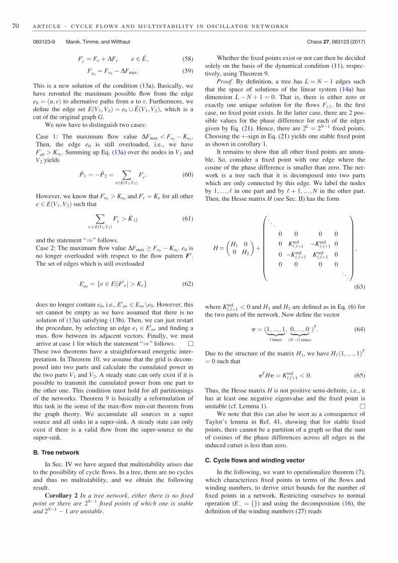
F0e ¼ Fe þ DFe e 2 ~E; (58)
F0e0¼ Fe0
DFmax: (59)
This is a new solution of the condition (13a). Basically, we
have rerouted the maximum possible flow from the edge
e0 ¼ ðu; vÞ to alternative paths from u to v. Furthermore, we
define the edge set EðV1;V2Þ ¼ e0 [ ~EðV1;V2Þ, which is a
cut of the original graph G.
We now have to distinguish two cases:
Case 1: The maximum flow value DFmax < Fe0 Ke0
.
Then, the edge e0 is still overloaded, i.e., we have
F0e0 > Ke0. Summing up Eq. (13a) over the nodes in V1 and
V2 yields
P1 ¼ P2 ¼X
e2EðV1;V2ÞF0e: (60)
However, we know that F0e0 > Ke0and F0e ¼ Ke for all other
e 2 EðV1;V2Þ such thatXe2EðV1;V2Þ
F0e > K12 (61)
and the statement “)” follows.
Case 2: The maximum flow value DFmax Fe0 Ke0
. e0 is
no longer overloaded with respect to the flow pattern F0.The set of edges which is still overloaded
E0ov ¼ fe 2 EjjF0ej > Keg (62)
does no longer contain e0, i.e., E0ov 2 Eovne0. However, this
set cannot be empty as we have assumed that there is no
solution of (13a) satisfying (13b). Then, we can just restart
the procedure, by selecting an edge e1 2 E0ov and finding a
max. flow between its adjacent vectors. Finally, we must
arrive at case 1 for which the statement “)” follows.
These two theorems have a straightforward energetic inter-
pretation. In Theorem 10, we assume that the grid is decom-
posed into two parts and calculate the cumulated power in
the two parts V1 and V2. A steady state can only exist if it is
possible to transmit the cumulated power from one part to
the other one. This condition must hold for all partitionings
of the networks. Theorem 9 is basically a reformulation of
this task in the sense of the max-flow min-cut theorem from
the graph theory. We accumulate all sources in a super
source and all sinks in a super-sink. A steady state can only
exist if there is a valid flow from the super-source to the
super-sink.
B. Tree network
In Sec. IV we have argued that multistability arises due
to the possibility of cycle flows. In a tree, there are no cycles
and thus no multistability, and we obtain the following
result.
Corollary 2 In a tree network, either there is no fixedpoint or there are 2N1 fixed points of which one is stableand 2N1 1 are unstable.
Whether the fixed points exist or not can then be decided
solely on the basis of the dynamical condition (11), respec-
tively, using Theorem 9.
Proof. By definition, a tree has L ¼ N 1 edges such
that the space of solutions of the linear system (14a) has
dimension L N þ 1 ¼ 0. That is, there is either zero or
exactly one unique solution for the flows Fj;‘. In the first
case, no fixed point exists. In the latter case, there are 2 pos-
sible values for the phase difference for each of the edges
given by Eq. (21). Hence, there are 2L ¼ 2N1 fixed points.
Choosing theþ-sign in Eq. (21) yields one stable fixed point
as shown in corollary 1.
It remains to show that all other fixed points are unsta-
ble. So, consider a fixed point with one edge where the
cosine of the phase difference is smaller than zero. The net-
work is a tree such that it is decomposed into two parts
which are only connected by this edge. We label the nodes
by 1;…; ‘ in one part and by ‘þ 1;…;N in the other part.
Then, the Hesse matrix H (see Sec. II) has the form
H¼ H1 0
0 H2
þ
. ..
0 0 0 0
0 Kred‘;‘þ1 Kred
‘;‘þ1 0
0 Kred‘;‘þ1 Kred
‘;‘þ1 0
0 0 0 0
. ..
0BBBBBBBBBBB@
1CCCCCCCCCCCA;
(63)
where Kred‘;‘þ1 < 0 and H1 and H2 are defined as in Eq. (6) for
the two parts of the network. Now define the vector
v ¼ ð1;…; 1|fflfflfflzfflfflffl‘ times
; 0;…; 0|fflfflfflzfflfflfflðN‘Þ times
ÞT: (64)
Due to the structure of the matrix H1, we have H1ð1;…; 1ÞT¼ 0 such that
vTHv ¼ Kred‘;‘þ1 < 0: (65)
Thus, the Hesse matrix H is not positive semi-definite, i.e., it
has at least one negative eigenvalue and the fixed point is
unstable (cf. Lemma 1).
We note that this can also be seen as a consequence of
Taylor’s lemma in Ref. 41, showing that for stable fixed
points, there cannot be a partition of a graph so that the sum
of cosines of the phase differences across all edges in the
induced cutset is less than zero.
C. Cycle flows and winding vector
In the following, we want to operationalize theorem (7),
which characterizes fixed points in terms of the flows and
winding numbers, to derive strict bounds for the number of
fixed points in a network. Restricting ourselves to normal
operation (E ¼ fg) and using the decomposition (16), the
definition of the winding numbers (27) reads
083123-9 Manik, Timme, and Witthaut Chaos 27, 083123 (2017)
70 article – cycle flows and multistability in oscillator networks
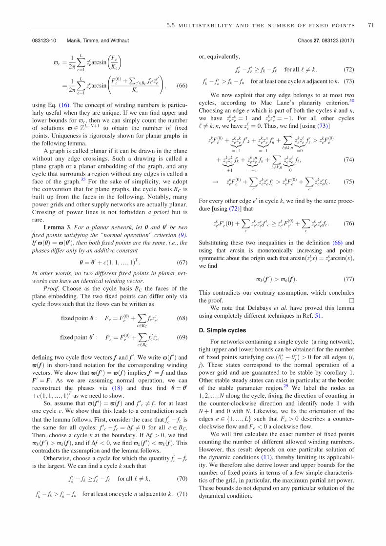
-c ¼1
2p
XL
e¼1
zcearcsin
Fe
Ke
¼ 1
2p
XL
e¼1
zcearcsin
F 0ð Þe þ
Pc02BC
fc0zc0e
Ke
!; (66)
using Eq. (16). The concept of winding numbers is particu-
larly useful when they are unique. If we can find upper and
lower bounds for -c, then we can simply count the number
of solutions - 2 ZLNþ1 to obtain the number of fixed
points. Uniqueness is rigorously shown for planar graphs in
the following lemma.
A graph is called planar if it can be drawn in the plane
without any edge crossings. Such a drawing is called a
plane graph or a planar embedding of the graph, and any
cycle that surrounds a region without any edges is called a
face of the graph.35 For the sake of simplicity, we adopt
the convention that for plane graphs, the cycle basis BC is
built up from the faces in the following. Notably, many
power grids and other supply networks are actually planar.
Crossing of power lines is not forbidden a priori but is
rare.
Lemma 3. For a planar network, let h and h0 be twofixed points satisfying the “normal operation” criterion (9).If -ðhÞ ¼ -ðh0Þ, then both fixed points are the same, i.e., thephases differ only by an additive constant
h ¼ h0 þ cð1; 1;…; 1ÞT : (67)
In other words, no two different fixed points in planar net-works can have an identical winding vector.
Proof. Choose as the cycle basis BC the faces of the
plane embedding. The two fixed points can differ only via
cycle flows such that the flows can be written as
fixed point h : Fe ¼ Fð0Þe þXc2BC
fczce; (68)
fixed point h0 : F0e ¼ Fð0Þe þXc2BC
fc0zc
e; (69)
defining two cycle flow vectors f and f 0. We write -ðf 0Þ and
-ðf Þ in short-hand notation for the corresponding winding
vectors. We show that -ðf 0Þ ¼ -ðf Þ implies f 0 ¼ f and thus
F0 ¼ F. As we are assuming normal operation, we can
reconstruct the phases via (18) and thus find h ¼ h0
þcð1; 1;…; 1ÞT as we need to show.
So, assume that -ðf 0Þ ¼ -ðf Þ and f 0c 6¼ fc for at least
one cycle c. We show that this leads to a contradiction such
that the lemma follows. First, consider the case that f0c fc is
the same for all cycles: f 0c fc ¼ Df 6¼ 0 for all c 2 BC.
Then, choose a cycle k at the boundary. If Df > 0, we find
-kðf 0Þ > -kðf Þ, and if Df < 0, we find -kðf 0Þ < -kðf Þ. This
contradicts the assumption and the lemma follows.
Otherwise, choose a cycle for which the quantity f0c fc
is the largest. We can find a cycle k such that
f 0k fk f 0‘ f‘ for all ‘ 6¼ k; (70)
f 0k fk > f 0n fn for at least one cycle n adjacent to k: (71)
or, equivalently,
f 0k f 0‘ fk f‘ for all ‘ 6¼ k; (72)
f 0k f 0n > fk fn for at least one cycle n adjacent to k: (73)
We now exploit that any edge belongs to at most two
cycles, according to Mac Lane’s planarity criterion.50
Choosing an edge e which is part of both the cycles k and n,
we have zkezk
e ¼ 1 and zkezn
e ¼ 1. For all other cycles
‘ 6¼ k; n, we have z‘e ¼ 0. Thus, we find [using (73)]
zkeFð0Þe þ zk
ezke|z
¼þ1
f 0k þ zkezn
e|z¼1
f 0n þX‘6¼k;n
zkez‘e|z¼0
f 0‘ > zkeFð0Þe
þ zkezk
e|z¼þ1
fk þ zkezn
e|z¼1
fn þX‘ 6¼k;n
zkez‘e|z¼0
f‘; (74)
! zkeFð0Þe þ
Xc
zkezc
e f 0c > zkeFð0Þe þ
Xc
zkezc
efc: (75)
For every other edge e0 in cycle k, we find by the same proce-
dure [using (72)] that
zke0F
0eð0Þ þ
Xc
zke0z
ce0 f0c zk
e0Fð0Þe0 þ
Xc
zke0z
ce0 fc: (76)
Substituting these two inequalities in the definition (66) and
using that arcsin is monotonically increasing and point-
symmetric about the origin such that arcsinðzkexÞ ¼ zk
earcsinðxÞ,we find
-kðf 0Þ > -kðf Þ: (77)
This contradicts our contrary assumption, which concludes
the proof.
We note that Delabays et al. have proved this lemma
using completely different techniques in Ref. 51.
D. Simple cycles
For networks containing a single cycle (a ring network),
tight upper and lower bounds can be obtained for the number
of fixed points satisfying cos ðhi hj Þ > 0 for all edges (i,j). These states correspond to the normal operation of a
power grid and are guaranteed to be stable by corollary 1.
Other stable steady states can exist in particular at the border
of the stable parameter region.29 We label the nodes as
1; 2;…;N along the cycle, fixing the direction of counting in
the counter-clockwise direction and identify node 1 with
Nþ 1 and 0 with N. Likewise, we fix the orientation of the
edges e 2 f1;…; Lg such that Fe > 0 describes a counter-
clockwise flow and Fe < 0 a clockwise flow.
We will first calculate the exact number of fixed points
counting the number of different allowed winding numbers.
However, this result depends on one particular solution of
the dynamic conditions (11), thereby limiting its applicabil-
ity. We therefore also derive lower and upper bounds for the
number of fixed points in terms of a few simple characteris-
tics of the grid, in particular, the maximum partial net power.
These bounds do not depend on any particular solution of the
dynamical condition.
083123-10 Manik, Timme, and Witthaut Chaos 27, 083123 (2017)
5.5 multistability and the number of fixed points 71

Remark 11. For any ring network RN with N nodes, thecycle flow vector defined in (2) and the winding vectordefined in (29) naturally reduce into single numbers. Werefer to them as cycle flow fc and winding number -c, follow-ing Ref. 39. These two quantities will be crucial in establish-ing the results in the rest of this section.
Theorem 12. For a ring network RN, the number ofnormal operation fixed points (denoted by N ) is given by
N ¼ 1
2p
Xj
arcsinF 0ð Þ
jþ1;j þ f maxc
Kjþ1;j
!& ’
1
2p
Xj
arcsinF 0ð Þ
jþ1;j þ f minc
Kjþ1;j
!$ % 1; (78)
where bc denotes the floor function and de denotes the ceil-ing function. F
ð0Þij is one particular solution to the dynamic
condition (11) and
f maxc ¼ min
jðKjþ1;j F
ð0Þjþ1;jÞ;
f minc ¼ max
jðKjþ1;j F
ð0Þjþ1;jÞ: (79)
Proof. Suppose that we have one fixed point h0 with the
flows Fð0Þij and analyze (as per Theorem 3) which cycle flow
values fc lead to different valid fixed points. First, the cycle
flow bounds both above and below since the flow Fj;jþ1 along
each edge cannot exceed in absolute value the capacity Kj;jþ1
f minc < fc < f max
c ; (80)
f maxc ¼ min
jðKj;jþ1 F
ð0Þj;jþ1Þ; (81)
f minc ¼ max
jðKj;jþ1 F
ð0Þj;jþ1Þ: (82)
We emphasize that fc cannot be equal to f maxc or f min
c because
otherwise one edge would be fully loaded with cos ðhi hjÞ¼ 0, contradicting our assumption.
Second, all fixed points have to satisfy the geometric
condition (cf. Theorem 7)
-ðfcÞ 2 Z: (83)
Since we restrict ourselves to normal operation, the
winding number for a single cycle reads
- fcð Þ ¼1
2p
Xj
arcsinF 0ð Þ
jþ1;j þ fc
Kjþ1;j
!: (84)
Using the bound for the cycle flow strength (80) and the fact
that arcsin is a monotonically increasing function, we find
that the winding number is also bound by
-ðf minc Þ - -ðf max
c Þ: (85)
As the winding numbers are unique (see Lemma 3), the dis-
tinct fixed points correspond to the following values of the
winding number:
-fixedpoint ¼ b-ðf minc Þc þ 1; b-ðf min
c Þc þ 2;…; d-ðf maxc Þe 1:
(86)
Counting these values and inserting the values of f minc and
f maxc then yield the number of fixed points N .
For practical applications, it is desirable to determine
the number of fixed points from the properties of the network
alone, without referring to a particular solution Fð0Þ. To
obtain suitable bounds for the number of fixed points N , we
first define some properties which characterize the network.
Definition 13. For a ring network RN with N 2N
nodes indexed by 1; 2;…;N along the cycle, a fragment F i;j
is defined as the path starting at node i and ending at node j.For any fragment F i;j, the partial net power Pij is defined as
Pij ¼Xj
k¼i
Pk: (87)
and the maximal partial net power is defined as
Pmax ¼ maxi;j
Pi;j: (88)
This concept is illustrated in Fig. 5. Furthermore, we definethe maximum and minimum transmission capacities
Kmax ¼ maxj
Kjþ1;j and Kmin ¼ minj
Kjþ1;j: (89)
Lemma 4. For any ring fragment F i;j, the partial netpower is equal to the net outward flow
Pij ¼ Fjþ1;j Fi1;i (90)
and Pmax ¼ maxj
Fjþ1;j mini
Fi1;i : (91)
Lemma 4 is a formalization of energy conservation. The
net outward flow from a segment must equal the cumulated
power injections in the fragment. We then seek the fragment
maximizing the total flow exchanged with the rest of the
ring. We note that the definitions of Pij and Pmax appeared
previously in Ref. 51.
Corollary 3. For a ring network RN, the number of nor-mal operation fixed points (denoted by N ) is bound fromabove and below by
0 N 2N
4
þ 1 (92)
FIG. 5. The maximum partial net power Pmax in different ring networks.
083123-11 Manik, Timme, and Witthaut Chaos 27, 083123 (2017)
72 article – cycle flows and multistability in oscillator networks

and by
N
4
2Kmax Pmax
Kmin
N N
2p2Kmin Pmax
Kmax
1: (93)
Proof. According to Lemma 12, the number of fixed
points N is given by
N ¼ d-ðf maxc Þe b-ðf min
c Þc 1: (94)
We make use of the fact that the arcsin function is
bound, arcsinðxÞ 2 ½p=2;þp=2, such that
- f maxc
¼ 1
2p
XN
j¼1
arcsinF 0ð Þ
jþ1;j þ f maxc
Kjþ1;j
!<
N
4;
- f minc
¼ 1
2p
XN
j¼1
arcsinF 0ð Þ
jþ1;j þ f minc
Kjþ1;j
!> N
4: (95)
This proves the first part (92) of the corollary. To prove the
second part, we start from
d-ðf maxc Þ-ðf min
c Þe1N d-ðf maxc Þ-ðf min
c Þe: (96)
Now, one can obtain upper and lower bounds for all terms in
the sum using the trigonometric relation
x y arcsin xð Þ arcsin yð Þ p2
x yð Þ; (97)
which holds for all 1 y x 1. This yields
1
2p
Xj
Dfc
Kjþ1;j - f max
c
- f min
c
1
4
Xj
Dfc
Kjþ1;j; (98)
where we define Dfc ¼ f maxc f min
c . Furthermore, this quan-
tity can be bound as
Dfc ¼ minjðKjþ1;j F
ð0Þjþ1;jÞ max
jðKjþ1;j F
ð0Þjþ1;jÞ
2Kmin þminjðF
ð0Þjþ1;jÞ max
jðF
ð0Þjþ1;jÞ;
¼ 2Kmin þmaxjðFð0Þj;jþ1Þ max
jðF
ð0Þjþ1;jÞ;
¼ 2Kmin Pmax using ð92Þð Þ; (99)
such that the fraction in Eq. (98) becomes
Dfc
Kjþ1;j 2Kmin Pmax
Kmax
: (100)
In a similar way, we find
Dfc 2Kmax Pmax: (101)
Substituting these bounds into Eq. (98) yields
- f maxc
- f min
c
N
2p2Kmin Pmax
Kmax
;
- f maxc
- f min
c
N
4
2Kmax Pmax
Kmin
;
(102)
which combined with (96) completes the proof.
We note that the first part of this bound (92) had previ-
ously been shown by Ochab and Gora38 as well as by
Delabays et al.37
Corollary 4. For homogeneous rings RN, i.e., Ki;iþ1
¼ K, Eq. (93) simplifies to
N
p N Pmax
2Kp
1 N N
2 N Pmax
4K
: (103)
In particular, ring networks RN with N 4 do not havemultiple stable fixed points. Ring network RN with N 7
nodes will have multiple stable fixed points ðN 2Þ if
Pmax < 2Kmin 4pN
Kmax : (104)
These relations can be proven by simply evaluating the
bounds in Corollary 3.
Corollary 5. As K is decreased in a homogeneous ringnetwork, the fixed points with the largest infinity norm of theflows
jjFjj1 :¼ maxjjFj;jþ1j
will be the first ones to vanish.Proof. We can see from (95) that both -ðf max
c Þ and
-ðf minc Þ are monotonically increasing functions of f max
c and
f minc , respectively. According to (80), when K is decreased,
f maxc decreases and f min
c increases. The corollary follows.
We illustrate how the bounds scale with the connectivity
K and Pmax for a sample ring of size N¼ 16 in Fig. 6. We see
in Fig. 6(a) that increasing K results in more stable fixed
points. Whereas Fig. 6(b) demonstrates that if the power gen-
erators ðPj 0Þ are clustered together, then the system has
less fixed points, as opposed to the case where they are more
distributed.
FIG. 6. Upper and lower bounds for
the number of fixed points N for a
sample 16 element ring as a function
of (a) K ¼ Kj;jþ1 for all 1 j 16 atPmax ¼ 3 and (b) Pmax at K¼ 10.
083123-12 Manik, Timme, and Witthaut Chaos 27, 083123 (2017)
5.5 multistability and the number of fixed points 73

E. Complex networks
Obtaining bounds for the number of fixed points is hard
in general, as we cannot simply decompose a network into
single cycles, unless no two cycles of a network share an
edge. The difficulty arises because cycle flows in two faces
sharing one or more edges can cancel or enhance each other.
This is why one cannot simply multiply the bounds for a
number of fixed points for each cycle to obtain a bound for
the total number of fixed points for a network. We demon-
strate this using two examples.
1. Two cycle flows destroying each other
First, we show that even if all single cycles support (multi-
ple) fixed points in case they are isolated, the full network may
not have a single fixed point at all. This is illustrated in Fig. 7
for a network consisting of just two cycles. The network motifs
shown in panels (a) and (b) have 3 and 1 stable fixed points,
respectively, whereas the full network shown in panel (c) does
not have a stable fixed point. Isolated cycle 2, i.e., the network
shown in Fig. 7(b), has a stable fixed point, but two edges are
heavily loaded such that there is nearly no security margin and
no available capacity for cycle flows. Fusing the two cycles as
in Fig. 7(c) disturbs the geometric condition for both cycles.
To restore the geometric condition - 2 Z2, we would have to
add some cycle flows. But this is impossible in cycle 2 such
that there is no stable fixed point in the full network.
2. Two cycle flows getting created
So, we have seen that getting a lower bound for a num-
ber of fixed points of a general network is hard, as multiply-
ing lower bounds for each cycle in a cycle basis does not
yield a valid lower bound. Next, we will show why obtaining
a good upper bound is also hard.
Consider any of the two identical single loop networks in
Fig. 8. It consists of one generator and one consumer, generat-
ing and consuming 2:1K power, respectively. Each edge has
capacity K. None of the two single loop networks have any
fixed point: simply because the network does not have enough
capacity to transport the 2:1K amount of power from the
generator to the consumer. However, when those two are fused
together, two cycle flows emerge and a stable fixed point with
winding vector x ¼ ð1;1Þ comes into existence. This should
not come as a surprise: fusing two cycles in this case ended up
with an alternate pathway for the powerflow being created.
F. Planar networks
Although obtaining estimates for a number of fixed
points for general topologies is quite difficult, we now show
that for planar topologies, it is possible to obtain some ana-
lytical insights.
1. Upper bound
Theorem 14. Consider a finite planar network. Choosethe faces of the graph as the cycle basis BC. Then, the numberof normal operation fixed points, i.e., fixed points satisfyingcos ðhi hj Þ > 0 for all edges (i, j), is bound from above by
N <YLNþ1
c¼1
2Nc
4
þ 1; (105)
where Nc is the number of nodes in cycle c.
Proof. In a planar network, no two different fixed points
can have the same winding vector - (see Lemma 3) such
that we can just count the different allowed winding vectors.
For each fundamental cycle c 2 BC, we have
bNc=4c < -c ¼1
2p
Xe2 cycle c
De < þbNc=4c (106)
because p=2 < De < þp=2 in normal operation. Counting
the number of different possible values of the winding num-
bers -1;…;-LNþ1 respecting these upper and lower bounds
yields the result.
Delabays et al. have presented37 this bound in the case
of uniform power injections Pj at all nodes. They have also
determined topological conditions that are sufficient to
ensure that all fixed points are under normal operation, thus
making the upper bound in (105) valid for all fixed points in
a certain class of networks.
FIG. 7. Difficulties in finding bound
for the number of stable fixed points in
the complex network. The network
motifs shown in (a) and (b) have 3 and
1 stable fixed points, respectively,
whereas the fused network shown in
(c) has no stable fixed point at all. The
power injections Pj are given in the
nodes. All edges have transmission
capacity K.
FIG. 8. Two ring networks, each with
no fixed point, when merged by an
edge, gain a fixed point.
083123-13 Manik, Timme, and Witthaut Chaos 27, 083123 (2017)
74 article – cycle flows and multistability in oscillator networks

Intriguingly, this upper bound has been demonstrated to
be invalid51 outside normal operation.
2. Asymptotic behaviour
We have shown in Subsection V E that it is not straight-
forward to obtain bounds for the number of fixed points Nin complex networks, unlike simple cycles. However, in the
limit of N 1;K 1, we can nevertheless derive the scal-
ing behaviour for N .
3. Two-cycle network
For simplicity, we first consider a network with homoge-
neous transmission capacities consisting of two cycles C1 and
C2, as illustrated in Fig. 9. Suppose that there are n1 edges
belonging only to cycle 1, n2 edges belonging only to cycle 2
and n12 edges belonging to both. Let one fixed point be h
with flows in each cycle and the intersection be bound by
Fmin1 Fe Fmax
1 ; for all e 2 C1 C2 (107)
Fmin2 Fe Fmax
2 ; for all e 2 C2 C1 (108)
Fmin12 Fe Fmax
12 ; for all e 2 C2 C1: (109)
Then, the possible cycle flows in each cycle are bound
inside a convex polygon D described by
K Fmin1 f1 K Fmax
1 ; (110)
K Fmin2 f2 K Fmax
2 ; (111)
K Fmin12 f1 f2 K Fmax
12 : (112)
Then, for K 1; n1 1; n2 1, the number of fixed
points converges to the area of the image set of D under the
mapping -.
N ð
-ðDÞd-1d-2; (113)
¼ðD
df1df2detJð-Þ; (114)
where the Jacobian Jð-Þ for the change in the variable
can be computed from the expression for - in (66), which
yields
detJ -ð Þ¼1
4K2p2
det
Xe2C1
1ffiffiffiffiffiffiffiffiffiffiffiffiffiffiffiffiffiffiffiffiffiffiffiffiffiffiffiffiffi1 Feþ f1
K
2s þ
Xe2C1\C2
1ffiffiffiffiffiffiffiffiffiffiffiffiffiffiffiffiffiffiffiffiffiffiffiffiffiffiffiffiffiffiffiffiffiffiffiffiffi1 Feþ f1 f2
K
2s
Xe2C1\C2
1ffiffiffiffiffiffiffiffiffiffiffiffiffiffiffiffiffiffiffiffiffiffiffiffiffiffiffiffiffiffiffiffiffiffiffiffiffi1 Feþ f1 f2
K
2s
X
e2C1\C2
1ffiffiffiffiffiffiffiffiffiffiffiffiffiffiffiffiffiffiffiffiffiffiffiffiffiffiffiffiffiffiffiffiffiffiffiffiffi1 Feþ f1 f2
K
2s X
e2C2
1ffiffiffiffiffiffiffiffiffiffiffiffiffiffiffiffiffiffiffiffiffiffiffiffiffiffiffiffiffi1 Feþ f2
K
2s þ
Xe2C1\C2
1ffiffiffiffiffiffiffiffiffiffiffiffiffiffiffiffiffiffiffiffiffiffiffiffiffiffiffiffiffiffiffiffiffiffiffiffiffi1 Feþ f1 f2
K
2s
0BBBBBBBBBB@
1CCCCCCCCCCA:
(115)
Taking the limitslim
K!1
Fe þ f1
K¼ f1
K;
limK!1
Fe þ f2
K¼ f2
K; (116)
leads to
N 1
4K2p2
ð~D
df1df2det
n1ffiffiffiffiffiffiffiffiffiffiffiffiffiffiffiffiffiffiffiffiffi1 f1
K
2s þ n12ffiffiffiffiffiffiffiffiffiffiffiffiffiffiffiffiffiffiffiffiffiffiffiffiffiffiffiffiffiffi
1 f1 f2K
2s n12ffiffiffiffiffiffiffiffiffiffiffiffiffiffiffiffiffiffiffiffiffiffiffiffiffiffiffiffiffiffi
1 f1 f2
K
2s
n12ffiffiffiffiffiffiffiffiffiffiffiffiffiffiffiffiffiffiffiffiffiffiffiffiffiffiffiffiffiffi1 f1 f2
K
2s n2ffiffiffiffiffiffiffiffiffiffiffiffiffiffiffiffiffiffiffiffiffi
1 f2K
2s þ n12ffiffiffiffiffiffiffiffiffiffiffiffiffiffiffiffiffiffiffiffiffiffiffiffiffiffiffiffiffiffi
1 f1 f2
K
2s
0BBBBBBBBB@
1CCCCCCCCCA:
~D : ¼ f f1; f2ð Þ : f1; f2ð Þ 2 R2; jf1j K; jf2j K; jf1 f2j Kg: (117)
FIG. 9. A 2-cycle network. We use the convention that cycles are counter-
clockwise. Therefore, we assign positive magnitudes to counter-clockwise
cycle flows and negative magnitudes to clockwise cycle flows.
083123-14 Manik, Timme, and Witthaut Chaos 27, 083123 (2017)
5.5 multistability and the number of fixed points 75

Redefining f1 ! f1=K; f2 ! f2=K, we obtain
N 1
4p2
ð~D
df1df2det
n1ffiffiffiffiffiffiffiffiffiffiffiffiffi1 f 2
1
p þ n12ffiffiffiffiffiffiffiffiffiffiffiffiffiffiffiffiffiffiffiffiffiffiffiffiffiffiffi1 f1 f2ð Þ2
q n12ffiffiffiffiffiffiffiffiffiffiffiffiffiffiffiffiffiffiffiffiffiffiffiffiffiffiffi1 f1 f2ð Þ2
q n12ffiffiffiffiffiffiffiffiffiffiffiffiffiffiffiffiffiffiffiffiffiffiffiffiffiffiffi
1 f1 f2ð Þ2q n2ffiffiffiffiffiffiffiffiffiffiffiffiffi
1 f 22
p þ n12ffiffiffiffiffiffiffiffiffiffiffiffiffiffiffiffiffiffiffiffiffiffiffiffiffiffiffi1 f1 f2ð Þ2
q0BBBB@
1CCCCA; (118)
¼ 1
4p2n1n2
ð~D
1ffiffiffiffiffiffiffiffiffiffiffiffiffi1 f 2
1
p 1ffiffiffiffiffiffiffiffiffiffiffiffiffi1 f 2
2
p df1df2 þ n1n12
ð~D
1ffiffiffiffiffiffiffiffiffiffiffiffiffi1 f 2
1
p 1ffiffiffiffiffiffiffiffiffiffiffiffiffiffiffiffiffiffiffiffiffiffiffiffiffiffiffi1 f1 f2ð Þ2
q df1df2
0@
þ n2n12
ð~D
1ffiffiffiffiffiffiffiffiffiffiffiffiffi1 f 2
2
p 1ffiffiffiffiffiffiffiffiffiffiffiffiffiffiffiffiffiffiffiffiffiffiffiffiffiffiffi1 f1 f2ð Þ2
q df1df2
1CA; (119)
¼ 1
4p2n1n2
ð~D
1ffiffiffiffiffiffiffiffiffiffiffiffiffi1 f 2
1
p 1ffiffiffiffiffiffiffiffiffiffiffiffiffi1 f 2
2
p df1df2 þ n1 þ n2ð Þn12
ð~D
1ffiffiffiffiffiffiffiffiffiffiffiffiffi1 f 2
1
p 1ffiffiffiffiffiffiffiffiffiffiffiffiffiffiffiffiffiffiffiffiffiffiffiffiffiffiffi1 f1 f2ð Þ2
q df1df2
0@
1A: (120)
In the last line, we use the symmetry in f1 and f2, both in the integrand and the domain of integration. We can simplify
even further, by using the following change in variables in the second integral:
ðf1; f2Þ7!ðf2 f1; f2Þ:We note that the domain remains the same after this change in the variable and the determinant of the Jacobian
detðJÞ ¼ 1. This allows the simplification
N n1n2 þ n1 þ n2ð Þn12ð Þ 1
4p2
ð~D
1ffiffiffiffiffiffiffiffiffiffiffiffiffi1 f 2
1
p 1ffiffiffiffiffiffiffiffiffiffiffiffiffi1 f 2
2
p df1df2|fflfflfflfflfflfflfflfflfflfflfflfflfflfflfflfflfflfflfflfflfflfflfflfflfflfflfflzfflfflfflfflfflfflfflfflfflfflfflfflfflfflfflfflfflfflfflfflfflfflfflfflfflfflfflc
;
with
c ¼ 1
4p2
ð0
1
df1ffiffiffiffiffiffiffiffiffiffiffiffiffi1 f 2
1
p ðf1þ1
1
df2ffiffiffiffiffiffiffiffiffiffiffiffiffi1 f 2
2
p þð1
0
df1ffiffiffiffiffiffiffiffiffiffiffiffiffi1 f 2
1
p ð1
f11
df2ffiffiffiffiffiffiffiffiffiffiffiffiffi1 f 2
2
p( )
;
¼ 1
4p2
ð0
1
arcsin f1 þ 1ð Þ þ p2ffiffiffiffiffiffiffiffiffiffiffiffiffi
1 f 21
p df1 þð1
0
p2 arcsin f1 1ð Þffiffiffiffiffiffiffiffiffiffiffiffiffi
1 f 21
p df1
8<:
9=;;
¼ 1
4p2
p2
4þð0
1
arcsin f1 þ 1ð Þffiffiffiffiffiffiffiffiffiffiffiffiffi1 f 2
1
p df1 þp2
4þð1
0
arcsin f1 1ð Þffiffiffiffiffiffiffiffiffiffiffiffiffi1 f 2
1
p df1
( );
¼ 1
8þ 1
2p2
ð0
1
arcsin f1 þ 1ð Þffiffiffiffiffiffiffiffiffiffiffiffiffi1 f 2
1
p df1;
0:1576;
to finally yield this scaling result
limn1;n2!1
N ¼ cðn1n2 þ ðn1 þ n2Þn12Þ; (121)
c 0:1576:
To evaluate the accuracy of (121), we apply it to two
special cases. First, we consider networks with n ¼ n1 ¼ n2;n12 ¼ 1, i.e., two identical cycles sharing only one single
edge. In this case, (121) becomes
Nðn; n; 1Þ ðn2 þ 2nÞc: (122)
Second, we consider networks with n ¼ n1 ¼ n2; n12 ¼ n,
i.e., two identical cycles sharing half of their edges. In this
case, (121) becomes
Nðn; n; nÞ 3cn2: (123)
We see in Fig. 10 that in both these cases, the scaling
relations are quite accurate even for not very large network
sizes, such as n¼ 50.
4. General planar graphs
The scaling results for two-cycle networks can be
extended to general planar graphs; to this end, we define a
few quantities.
Definition 15 (Loopy dual graph). Given a planar graphG(V, E) and an embedding, we choose a cycle basis BC con-sisting of the faces of the embedding. The loopy dual graphGdualðGÞ is an undirected multigraph whose vertex set isequal to BC. Its edge set E0 is as follows. For each edge
083123-15 Manik, Timme, and Witthaut Chaos 27, 083123 (2017)
76 article – cycle flows and multistability in oscillator networks

e 2 E, if it is shared between two cycles c1 and c2, then anedge between c and c0 is added to E0. If e is at the boundaryand belongs to only one cycle c, then a self-loop is added atnode c. We illustrate this definition in Fig. 11.
Now, consider a planar graph and an arbitrarily chosen
fixed point with flows Fe. Let us denote by ~Lloopy
the loopy
Laplacian of its metagraph, as defined in Definition 1.
Then, Eq. (117) generalizes to
N 1
2Kpð ÞLNþ1
ð~D
df1df2 dfLNþ1det ~Lloopy
; (124)
~D :¼ fðf1; f2;…fLNþ1Þ : jfij K; jfi fjj K
if cycles i; j share an edgeg:
VI. UNSTABLE FIXED POINTS
In principle, we can generalize the cycle flow approach
to find fixed points which do not satisfy the normal operation
condition, too. These fixed points are typically linearly
unstable (cf. the discussion in Ref. 30) However, most of the
results on the number of fixed points cannot be generalized
to this case. As an instructive example, consider again a
homogeneous ring as in Sec. IV C. We label the nodes as
1; 2;…;N along the cycle and assume that N is an integer
multiple of 4. All nodes have a vanishing power injection
Pj 0, and all links have an equal strength K as before.
Then, it is easy to see that
h ¼ ð0; d; p; pþ d; 2p; 2pþ d; 3p;…ÞT (125)
is a fixed point of the dynamics for each value of d 2 ½0; pÞ.This class of fixed points represents a pure cycle flow
Fj;jþ1 ¼ K sin ðhjþ1 hjÞ ¼ K sin ðdÞ (126)
for all edges ðj; jþ 1Þ. The winding number is - ¼ N=4
independent of the value of d and the edges belong alter-
nately to Eþ and E
Eþ ¼ fð1; 2Þ; ð3; 4Þ; ð5; 6Þ; …g;E ¼ fð2; 3Þ; ð4; 5Þ; ð6; 7Þ; …g: (127)
This simple example shows that two main assumptions
made for the normal operation fixed points (where E ¼ fg)do not longer hold: first, the set of fixed points is no longer dis-
crete. Instead, we find a continuum of solutions parametrized
by the real number d. Second, different fixed points yield the
same winding number. Thus, we cannot obtain the number of
fixed points by counting winding numbers in general.
VII. CALCULATING ALL FIXED POINTS
The cycle flow approach yields a convenient method to
calculate multiple fixed points for oscillator networks.
FIG. 10. (a) Scaling of the number of fixed points for two-cycle networks at zero power injection and infinite edge capacity limit. (a) Each cycle has nþ 1
edges, and they share one edge between them. (Left y-axis) The dots show the exact number of fixed points computed numerically. The solid line shows the
predicted number as per scaling relation (121). The dashed line shows the upper bound (105). (Right y-axis) The dotted line shows the number of fixed points
divided by n2 þ 2n converging to a constant value, that is close to the analytically predicted value c ¼ 0:1576, as per equation (121). (b) The same as (a), but
for networks where each cycle has 2n edges, they share n edges between them.
FIG. 11. A planar graph (solid edges, unfilled circular nodes) and its loopy
dual (dashed edges, filled circular nodes) corresponding to this specific
embedding.
083123-16 Manik, Timme, and Witthaut Chaos 27, 083123 (2017)
5.6 unstable fixed points 77
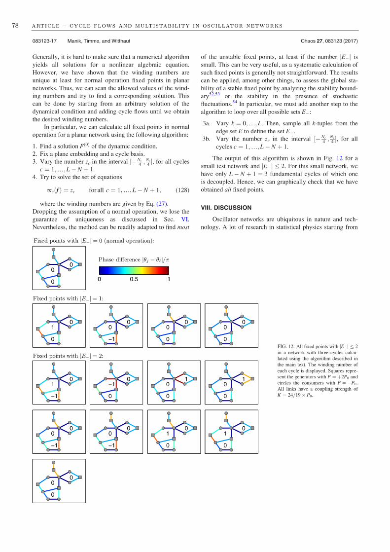
Generally, it is hard to make sure that a numerical algorithm
yields all solutions for a nonlinear algebraic equation.
However, we have shown that the winding numbers are
unique at least for normal operation fixed points in planar
networks. Thus, we can scan the allowed values of the wind-
ing numbers and try to find a corresponding solution. This
can be done by starting from an arbitrary solution of the
dynamical condition and adding cycle flows until we obtain
the desired winding numbers.
In particular, we can calculate all fixed points in normal
operation for a planar network using the following algorithm:
1. Find a solution Fð0Þ of the dynamic condition.
2. Fix a plane embedding and a cycle basis.
3. Vary the number zc in the interval ½ Nc
4; Nc
4, for all cycles
c ¼ 1;…; L N þ 1.
4. Try to solve the set of equations
-cðf Þ ¼ zc for all c ¼ 1;…; L N þ 1; (128)
where the winding numbers are given by Eq. (27).
Dropping the assumption of a normal operation, we lose the
guarantee of uniqueness as discussed in Sec. VI.
Nevertheless, the method can be readily adapted to find most
of the unstable fixed points, at least if the number jEj is
small. This can be very useful, as a systematic calculation of
such fixed points is generally not straightforward. The results
can be applied, among other things, to assess the global sta-
bility of a stable fixed point by analyzing the stability bound-
ary52,53 or the stability in the presence of stochastic
fluctuations.54 In particular, we must add another step to the
algorithm to loop over all possible sets E:
3a. Vary k ¼ 0;…; L. Then, sample all k-tuples from the
edge set E to define the set E.
3b. Vary the number zc in the interval ½ Nc
4; Nc
4, for all
cycles c ¼ 1;…; L N þ 1.
The output of this algorithm is shown in Fig. 12 for a
small test network and jEj 2. For this small network, we
have only L N þ 1 ¼ 3 fundamental cycles of which one
is decoupled. Hence, we can graphically check that we have
obtained all fixed points.
VIII. DISCUSSION
Oscillator networks are ubiquitous in nature and tech-
nology. A lot of research in statistical physics starting from
FIG. 12. All fixed points with jEj 2
in a network with three cycles calcu-
lated using the algorithm described in
the main text. The winding number of
each cycle is displayed. Squares repre-
sent the generators with P ¼ þ2P0 and
circles the consumers with P ¼ P0.
All links have a coupling strength of
K ¼ 24=19 P0.
083123-17 Manik, Timme, and Witthaut Chaos 27, 083123 (2017)
78 article – cycle flows and multistability in oscillator networks

Kuramoto’s seminal work2 has been devoted to the onset of
partial synchronization in large networks. However, in some
applications, global synchronization is required. In particu-
lar, in electrical power grids, all generators have to run with
exactly the same frequency and have to be strictly phase-
locked to enable stable power flows to the customers. A
desynchronization generally has catastrophic consequences.
An example is provided by the European power blackout in
November 2006. Following a shutdown of one transmission
line and unsuccessful attempts to restore stable operation,
the European grid fragmented in three mutually asynchro-
nous clusters.23 In the end, more than 10 million customers
were cut from the power supply.
In this article, we have analyzed the existence of stable
fixed points in finite oscillator networks. The main methodo-
logical advancement is to split the calculation into two parts:
first, we calculate the flows which satisfy the continuity
equation at all nodes. Then, we single out the specific solu-
tion which leads to consistent phases of the oscillators. We
thus move the focus of the calculation from the nodes
(phases) to the edges (flows) and cycles. An immediate con-
sequence is that several fixed points can co-exist, which dif-
fer by cycle flows. Thus, oscillator networks are in general
multistable.
For networks containing a single cycle, we have
obtained upper and lower bounds for the number of fixed
points in terms of three structural quantities: the maximal
partial net power Pmax, which measures the homogeneity of
the power injections or natural frequencies and the maximum
and minimum edge strength along the cycle. We find that
generally the number of stable fixed points is particularly
large if (a) the cycle is long, (b) the edge strength is large,
and (c) the power sources are distributed homogeneously.
However, the example discussed in Sec. IV D shows that
extreme care has to be taken for special network topologies.
Increasing the strength of the wrong edge can also decrease
the number of fixed points. Finding bounds for the number
of stable fixed points in general network topologies is much
more involved. The results have been obtained for planar
networks, but the bounds are much weaker as for networks
with single cycles. Interestingly, both tree networks and fully
connected networks have at most one stable fixed point.
However, networks with intermediate sparsity, which is
most realistic for electrical power grids, may exhibit
multistability.
Several aspects of multistability have been previously
discussed in the literature. Multistability in isolated rings
was discussed in Ref. 38. The limits (92) were derived, and
the basins of attraction of the different fixed points were
studied numerically. The case of a densely connected graph
was analyzed by Taylor in Ref. 41. He was able to show that
there is at most one stable fixed point if the node degree is at
least 0:9395 ðN 1Þ. Mehta et al. investigate multistabil-
ity in complex networks numerically using a similar
approach to the present paper.43 They argue that the number
of fixed points scales with the number of cycles as each cycle
can accommodate cycle flows. While this is valid for many
graphs, there are counterexamples (Fig. 7). Delabays et al.37
have recently reported their treatment of multistability using
cycle flows. They have extended the upper bounds for fixed
points in single rings in Ref. 38 to also include those stable
fixed points with phase differences along edges >p=2. They
have also derived upper bounds51 for a number of fixed
points for planar graphs in the case of uniform power injec-
tions at all nodes. Xi et al.55 have numerically shown that the
spatial heterogeneity of power injections Pj reduces the num-
ber of fixed points, which fits with our analytical result in
Corollary 3. Intriguingly, they have also found that in hetero-
geneous ring topologies, the nonlinear stability of fixed
points decreases with the ring size N.
In this work, we have obtained a lower bound for the
number of fixed points and thereby provided a sufficient condi-tion for the existence of multistability. Furthermore, we have
shown that the length of the cycles Nc and the homogeneityPmax are equally important for multistability and thereby
arrived at tighter bounds for the number of fixed points than
Ochab and Gora38 and Delabays et al.37 Moreover, we have
derived scaling laws at the limit of infinite transmission
strengths that are much tighter than the upper bound results
previously reported. We have shown the derived scaling
behaviour to match numerically computed exact results for
moderately sized networks.
Interestingly, our results show that a previous highly rec-
ognized result presented by Jadbabaie et al. in Ref. 57 is incor-
rect. The authors claim that for any network of Kuramoto
oscillators with different natural frequencies, there exists a Ku
such that for K > Ku there is only one stable fixed point. This
claim is disproven by the examples presented in Sec. IV C as
well as by the rigorous results on the existence of multiple
fixed points in Corollary 3. The error in the proof of Ref. 57 is
rather technical. The authors define a function L such that the
defining equation of a fixed point (4) can be rewritten in the
form
h ¼ LðhÞ: (129)
Jadbabaie et al. then claim that L is a contraction on the sub-
set of h such that jhi hjj < p=2 for all edges (i, j), which
we called normal operation. Banach’s contraction theorem
then yields that the algebraic equation (129) has a unique
fixed point. The problem is that the range of LðhÞ is gener-
ally not a subset of subspace of normal operation, even if the
domain is. After applying L, some phase differences can get
out of the interval ½p=2; p=2. Thus, Banach’s contraction
theorem cannot be applied, which spoils the proof.
IX. CONCLUSION
In summary, taking cycle flows as a basis of flow pat-
terns, we analyzed the existence and stability of phase locked
states in networks of Kuramoto oscillators and second order
phase oscillators modeling the phase dynamics of electric
power grids. We demonstrated that such systems exhibit
multistability. Intriguingly, multistability prevails even under
conditions where unique stable operating points were
believed to exist in both a power engineering textbook and a
major complex network reference on Kuramoto oscilla-
tors.56,57 For classes of network topologies, we have estab-
lished necessary and sufficient conditions for multistability
083123-18 Manik, Timme, and Witthaut Chaos 27, 083123 (2017)
5.9 conclusion 79
and derived lower and upper bounds for the number of fixed
points. We explained why generalizing those bounds for
arbitrary topologies is hard. Nevertheless, we have derived
asymptotic scaling laws at a large loop limit that has been
found to match closely numerically obtained exact results.
ACKNOWLEDGMENTS
We gratefully acknowledge support from the Federal
Ministry of Education and Research (BMBF Grant No.
03SF0472A-E), the Helmholtz Association (via the joint
initiative “Energy System 2050 – A Contribution of the
Research Field Energy” and the Grant No. VH-NG-1025 to
D.W.) and the Max Planck Society to M.T. The works of
D.M. were supported by the IMPRS Physics of Biological
and Complex Systems, G€ottingen.
1C. Huygens, Oeuvres Completes de Christiaan Huygens (Martinus
Nijhoff, The Hague, The Netherlands, 1893).2Y. Kuramoto, in International Symposium on Mathematical Problems inTheoretical Physics, Lecture Notes in Physics Vol. 39, edited by H. Araki
(Springer, New York, 1975), p. 420.3Y. Kuramoto, Chemical Oscillations, Waves, and Turbulence (Springer,
Berlin, 1984).4K. Wiesenfeld, P. Colet, and S. H. Strogatz, Phys. Rev. Lett. 76, 404
(1996).5F. Varela, J.-P. Lachaux, E. Rodriguez, and J. Martinerie, Nat. Rev.
Neurosci. 2, 229 (2001).6I. Z. Kiss, Y. Zhai, and J. L. Hudson, Science 296, 1676 (2002).7S. H. Strogatz, Phys. D: Nonlinear Phenom. 143, 1 (2000).8J. A. Acebron, L. L. Bonilla, C. J. Perez Vicente, F. Ritort, and R. Spigler,
Rev. Mod. Phys. 77, 137 (2005).9A. Arenas, A. Dıaz-Guilera, J. Kurths, Y. Moreno, and C. Zhou, Phys.
Rep. 469, 93 (2008).10D. Witthaut and M. Timme, Phys. Rev. E 90, 032917 (2014).11B. Ermentrout, J. Math. Biol. 29, 571 (1991).12S.-Y. Ha, E. Jeong, and M.-J. Kang, Nonlinearity 23, 3139 (2010).13S. H. Strogatz, D. M. Abrams, A. McRobie, B. Eckhardt, and E. Ott,
Nature 438, 43 (2005).14A. R. Bergen and D. J. Hill, IEEE Trans. Power Appar. Syst. PAS-100, 25
(1981).15G. Filatrella, A. H. Nielsen, and N. F. Pedersen, Eur. Phys. J. B 61, 485
(2008).16M. Rohden, A. Sorge, M. Timme, and D. Witthaut, Phys. Rev. Lett. 109,
064101 (2012).17A. E. Motter, S. A. Myers, M. Anghel, and T. Nishikawa, Nat. Phys. 9,
191 (2013).18F. D€orfler, M. Chertkov, and F. Bullo, Proc. Natl. Acad. Sci. 110, 2005 (2013).19M. Rohden, A. Sorge, D. Witthaut, and M. Timme, Chaos 24, 013123 (2014).20B. Sch€afer, M. Matthiae, M. Timme, and D. Witthaut, New J. Phys. 17,
015002 (2015).21M. E. J. Newman, Networks—An Introduction (Oxford University Press,
Oxford, 2010).22D. Witthaut, M. Rohden, X. Zhang, S. Hallerberg, and M. Timme, Phys.
Rev. Lett. 116, 138701 (2016).
23Union for the Coordination of Transmission of Electricity, https://
www.entsoe.eu/fileadmin/user_upload/_library/publications/ce/otherreports/
Final-Report-20070130.pdf for Final report on the system disturbance;
accessed 4 November 2006 (2007).24S. Watanabe and S. H. Strogatz, Phys. Rev. Lett. 70, 2391 (1993).25C. Bick, M. Timme, D. Paulikat, D. Rathlev, and P. Ashwin, Phys. Rev.
Lett. 107, 244101 (2011).26G. Filatrella, N. F. Pedersen, and K. Wiesenfeld, Phys. Rev. E 61, 2513
(2000).27G. Filatrella, N. F. Pedersen, and K. Wiesenfeld, Phys. Rev. E 75, 017201
(2007).28S. Gupta, A. Campa, and S. Ruffo, J. Stat. Mech.: Theory Exp. 2014,
R08001.29D. Manik, D. Witthaut, B. Sch€afer, M. Matthiae, A. Sorge, M. Rohden, E.
Katifori, and M. Timme, Eur. Phys. J. Spec. Top. 223, 2527 (2014).30T. Coletta and P. Jacquod, Phys. Rev. E 93, 032222 (2016).31L. G. Khazin and E. Schnol, Stability of Critical Equilibrium States
(Manchester University Press, 1991).32C. J. Tavora and O. J. Smith, IEEE Trans. Power Appar. Syst. PAS-91,
1138–1144 (1972).33E. Katifori, G. J. Sz€ollosi, and M. O. Magnasco, Phys. Rev. Lett. 104,
048704 (2010).34H. Ronellenfitsch, M. Timme, and D. Witthaut, IEEE Trans. Power Syst.
32, 1007 (2016).35R. Diestel, Graph Theory (Springer, New York, 2010).36C. Godsil and G. F. Royle, Algebraic Graph Theory (Springer Science &
Business Media, 2013), Vol. 207.37R. Delabays, T. Coletta, and P. Jacquod, J. Math. Phys. 57, 032701 (2016).38J. Ochab and P. Gora, Acta Phys. Pol. Ser. B, Proc. Suppl. 3, 453 (2010).39D. A. Wiley, S. H. Strogatz, and M. Girvan, Chaos: Interdiscip. J.
Nonlinear Sci. 16, 015103 (2006).40M. Wolf, F. Verstraete, and J. Cirac, Int. J. Quantum Inf. 1, 465 (2003).41R. Taylor, J. Phys. A: Math. Theor. 45, 055102 (2012).42F. Ionita, D. Labavic, M. A. Zaks, and H. Meyer-Ortmanns, Eur. Phys. J.
B 86, 511 (2013).43D. Mehta, N. Daleo, F. D€orfler, and J. D. Hauenstein, Chaos 25, 053103
(2015).44A. Korsak, IEEE Trans. Power App. Syst. PAS-91, 1093 (1972).45D. Witthaut and M. Timme, New J. Phys. 14, 083036 (2012).46D. Witthaut and M. Timme, Eur. Phys. J. B 86, 377 (2013).47D. Braess, Unternehmensforschung 12, 258 (1968).48Y. Nussbaum, preprint arXiv:1012.4767 (2010).49L. R. Ford, Jr. and D. R. Fulkerson, Flows in Networks (Princeton
University Press, 2015).50S. Mac Lane, Fundam. Math. 28, 22 (1937).51R. Delabays, T. Coletta, and P. Jacquod, J. Math. Phys. 58, 032703 (2017).52P. J. Menck, J. Heitzig, N. Marwan, and J. Kurths, Nat. Phys. 9, 89 (2013).53H.-D. Chiang, F. Wu, and P. Varaiya, IEEE Trans. Circuits Syst. 34, 160
(1987).54B. Sch€afer, M. Matthiae, X. Zhang, M. Rohden, M. Timme, and D.
Witthaut, Phys. Rev. E 95, 060203 (2017).55K. Xi, J. L. Dubbeldam, and H. X. Lin, Chaos: Interdiscip. J. Nonlinear
Sci. 27, 013109 (2017).56A. Jadbabaie, N. Motee, and M. Barahona, in Proceedings of the 2004
American Control Conference (IEEE, 2004), Vol. 5, pp. 4296–4301.57J. Machowski, J. Bialek, and J. Bumby, Power System Dynamics, Stability
and Control (John Wiley & Sons, New York, 2008).58W. Chen, D. Wang, J. Liu, T. Basar, K. H. Johansson, and L. Qiu, IFAC-
PapersOnLine 49(22), 97–102 (2016).
083123-19 Manik, Timme, and Witthaut Chaos 27, 083123 (2017)
80 article – cycle flows and multistability in oscillator networks
6M A N U S C R I P T – B R A E S S ’ PA R A D OX I N
C O N T I N U O U S F L OW N E T WO R K S : A N E T WO R K
DY N A M I C S P E R S P E C T I V E
Debsankha Manik1, Marc Timme1,2,3, Dirk Witthaut4,5
1 Network Dynamics, Max Planck Institute for Dynamics and Self-
Organization (MPI DS), D-37077 Gottingen, Germany
2 Chair for Network Dynamics, Institute for Theoretical Physics
and Center for Advancing Electronics Dresden (cfaed), Technical
University of Dresden, 01069 Dresden, Germany
3 Department of Physics, Technical University Darmstadt, 64289
Darmstadt, Germany
4 Forschungszentrum Julich, Institute for Energy and Climate Re-
search – Systems Analysis and Technology Evaluation (IEK-STE),
52425 Julich, Germany
5 Institute for Theoretical Physics, University of Cologne, 50937
Koln, Germany
Original contribution:
I conceptualized the article and wrote the first draft of the manuscript.
I performed all the analytical calculations behind the results and all
numerical computations.

82 braess’ paradox in continuous flow networks
Abstract. Flow networks perform critical functions in various nat-
ural and man made systems, e.g. the venation networks in plant leaves
and the electrical power transmission grid. Such networks often under-
goes topological changes, both planned and unplanned: e.g. shutdowns
of power lines due to a storm or scheduled maintenance; or leaf veins
getting eaten through by bugs. It is therefore very important to under-
stand how such topological changes influence the flows in the network.
In the context of traffic networks, it was discovered by traffic engi-
neer D. Braess in 1968 that opening a new street in a street network
may increase travel time for everyone, if each car selfishly chooses
the fastest route for oneself. This phenomenon, subsequently named
“Braess’ paradox” (BP), has been later reported in various other flow
networks, including phase oscillator networks, linear flow networks
and discrete message passing networks. When a flow network needs
to carry more flow, it is a common strategy to strengthen an edge or
add new one. If BP is possible in a flow network, such an attempt
at improving the network may actually overload or destabilize it. Al-
though the prevalence of this phenomenon is well known, establishing
criteria for an edge in a given network to exhibit Braess’ paradox is
still an unsolved problem. In this article, we consider BP in a class
of flow networks that includes Kuramoto networks (that can be used
to model the AC power transmission grid) as well as linear flow net-
works (that can be used to model the fluid flow in leaf veins). Using
the notion of network susceptibilities, we take a differential view to
Braess’ paradox, defining BP as an increase in the maximum load on
infinitesimal increase of the strength of an edge. We reduce the prob-
lem of determining Braessian edges in a flow network to a simpler one
of determining the flows in the same network topology with a single-
source single-sink input. This results in a computational speedup by
a factor proportional to the number of edges in the network. More
importantly, this approach enables us to obtain a topological under-
standing of which edges are more likely to be Braessian. We use this
insight to establish topological classifiers for Braessian edges. Finally,
we demonstrate that Braessian edges have a beneficial effect : they
can be intentionally damaged to mitigate overload due to damage at
another edge.
6.1 introduction
Braess [32] demonstrated an intriguing phenomena in traffic networks,
where opening a new street in a traffic network leads to an increase
of the travel time for everyone. This happened because using the new
street was faster for each car compared to all other routes available to it,
leading to all cars to use this new street, which had the collective effect
of increasing travel time for every car. In other words, Braess’ para-
dox (BP) was a combined consequence of the network topology (which
6.1 introduction 83
allowed high utilization of the newly opened edge to bottleneck the net-
work) and the dynamics (each cars tried to maximize their individual
benefits in the selfish routing strategy).
Braess’ paradox in traffic networks
Subsequently, the topic of BP in selfish routing networks has been ex-
tensively explored. Frank [60] presented necessary and sufficient con-
ditions for BP in a 4-node single-source-single-link system, Steinberg
and Zangwill [33] as well as Dafermos and Nagurney [34] extended it to
general networks. Pas and Principio [35] showed that under non-selfish
routing strategies, BP does not occur, however adding a link may lead
to no better (nor worse) average performance. Valiant and Roughgar-
den [61] showed that in large random graphs, BP is not a rare event
and it occurs with high probability.
The topic of preventing Braess’ paradox has been studied in com-
puter networking literature [99, 100] and traffic engineering literature
[101]. However, given a flow network, determining which edges would
cause BP remains largely unsolved, apart from proofs [99, 100] that
certain extremely restricted class of line additions do not cause BP, e.g.
strengthening (i.e. increasing the edge capacity) the line directly join-
ing the source and sink in a single source/sink network and upgrading
all links in a network simultaneously.
Braess’ paradox in continuous flow networks
In a continuous flow network, e.g. a resistor network conducting elec-
tric current or venation networks in plant leaves transporting sap; the
dynamics is quite different from routing of discrete entities in street or
computer networks. Nevertheless, it has been reported that BP is preva-
lent in such networks, for example, in electrical circuits with resistors
and diodes [102, 103], oscillator networks and models of DC and AC
power grid [37, 36] as well as two-dimensional electron systems [104].
Scope and structure of this article
In this context, we ask this question: given a certain continuous flow
network, can we predict which edges will exhibit BP without explicitly
computing the flows after each edge perturbation? We emphasize that
we define Braess’ paradox as the maximum flow increasing on adding
or strengthening an edge, not the average flow or every flow increasing,
in contrast to traffic literature. We do so because increase of maximum
flow in a network is known to sometimes cause system wide failures
[105], when the initial overload starts a cascade. Coletta and Jacquod
[38] showed recently that it is possible to predict whether loads will
increase in an oscillator network with one-dimensional chain topology
84 braess’ paradox in continuous flow networks
if a pair of nodes previously unconnected is connected by an edge, from
previous steady state phases alone. In the present article, we attack
this question in arbitrary topologies and in a wider class of network
dynamics that includes both linear flow networks (describing flow of sap
in plant leaves and DC flow in a resistor network [14]) and Kuramoto
oscillator networks (used to model AC power transmission grid [19]).
In section 6.2, we provide a mathematical definition of BP in a class
of flow networks we call “conservative flow networks” and derive an
exact mapping between the problem of detecting Braessian edges in a
network and the problem of finding steady flows in a linear flow network
due to single dipole source (continuous version of which is familiar from
electrostatics). In section 6.3, we define an intuitive topological notion
of flow alignment and demonstrate that edges with flows aligned to the
maximally loaded edge are more likely to exhibit BP. In section 6.4,
we demonstrate that Braess’ paradox has a useful side effect: they can
be intentionally damaged to reverse an overload caused by damage at
another edge.
6.2 network susceptibility and braess’ paradox
This study on Braess’ paradox will be limited to conservative flow net-
works as per definition 2.2.4. Such systems include linear systems such
as electrical DC flow across a resistor network, flow of water in hydraulic
tubes, as well as flow of fluid in venation network in plant leaves [14, 18],
as well as nonlinear systems such as networks of Kuramoto oscillators
[1] as well as the swing equation model [19] of electrical AC transmission
grid.
We will now define Braess’ paradox on such systems, and derive
an exact mapping from the problem of finding Braessian edges to the
problem of finding steady flows in a linear flow network with a single
dipole source.
6.2.1 Mathematical background
We introduced the concept on network susceptibilities in [106] to quan-
tify the effect on steady state flows in a flow network (defined in section
2.2) on infinitesimally increasing the weight of an edge. We will now
define Braess’ paradox in terms of network susceptibilities.
Definition 6.2.1 (Edge-to-edge susceptibility). Consider a flow
network (G(V, E), I,F ) with steady state flows Fij for all i, j ∈ E.
Suppose on increasing the weight of a single edge µ := s, t from Kst
to Kst + κ, the steady state flows of another edge ν := i, j becomes F′ij.Then the edge-to-edge susceptibility is defined as
ηµ→ν := limκ→0
F′ν − Fν
κ=
dFν
dKµ=
dFij
dKst. (6.1)

6.2 network susceptibility and braess’ paradox 85
Definition 6.2.2 (Braessian edge). Consider a flow network (G, I,F ).
Suppose the maximum absolute flow is across the edge α
maxe∈E|Fe| = |Fα| .
Then an edge µ is called a Braessian edge (BE) if and only if
an infinitesimal increase in the weight of edge µ increases the absolute
value of the maximal flow Fα
Fαηµ→α > 0. (6.2)
Determining all BE’s in a network by Eq. (6.2) requires computing
the flow derivatives in Eq. (6.1) |E| times. We will now establish an
equivalent dual problem (that can be solved much faster) exploiting a
symmetry property of edge-to-edge susceptibilities for conservative flow
networks.
6.2.2 Edge-to-edge susceptibility in a conservative flow network
Consider a conservative flow network (G, I,F ). Due to the flow conser-
vation property Eq. (2.15), and the flow equation Eq. (2.10), the flows
at the edges must satisfy
∀1 ≤ j ≤ |V| , 0 = Ij + ∑i
Kij f (ϕi − ϕj). (6.3)
Suppose on increasing the weight of a single edge µ = s, t by κ,
the steady state vertex properties ϕj changes to ϕj + ξ j. Then the new
flows must still satisfy
0 =Ij + ∑i
(Kij + κδsiδtj + κδsjδti
)f (ϕi − ϕj + ξi − ξ j)
=Ij + κδtj f (ϕs − ϕj) + κδsj f (ϕt − ϕj) + ∑i
Kij(
f (ϕi − ϕj)
+ f ′(ϕi − ϕj)(ξi − ξ j))
+O((ξi − ξ j)
2) .
(6.4)
Subtracting Eq. (6.3):
0 =κδtj f (ϕs − ϕj) + κδsj f (ϕt − ϕj) + ∑i
Kij f ′(ϕi − ϕj)(ξi − ξ j)
+O((ξi − ξ j)
2) .(6.5)
We will now recast Eq. (6.5) in a form that is both more intuitive
and mathematically enlightening.
Definition 6.2.3 (Meta graph). Given a flow network (G, I,F ) with
flows Fij for all edges i, j ∈ E, a meta graph G is a graph with edge
set E and vertex set V, with edge weights given by
Kij = Kij f ′(ϕi − ϕj). (6.6)

86 braess’ paradox in continuous flow networks
We note that Kij = Kji because f ′ is an even function due to f being
odd. Furthermore, due to f being monotonically increasing function,
Kij ≥ 0. Therefore G is a valid weighted undirected graph with non-
negative weights.
Let L be the Laplacian matrix (see definition 2.1.12) of the meta
graph G of the original graph G, and M be incidence matrix (see def-
inition 2.1.11) of G and assume the edge s, t to be perturbed is the
µ’th one in the edge ordering considered while constructing M.
Then Eq. (6.5) can be rewritten as
Lijξ j = −κFst
Kst(δis − δit)
Lijdϕj
dKst= Lij lim
κ→0
ξ j
κ
= − Fst
Kst(δis − δit) .
(6.7)
This allows us to reformulate the edge to edge susceptibilities Eq. (6.1)
as
η(s,t)→(j,l) =dFjl
dKst= Kjl
(dϕl
dKst− dϕj
dKst
),
Lijdϕj
dKst= − Fst
Kst(δis − δit) .
(6.8)
We will now demonstrate that the edge-to-edge susceptibilities η(s,t)→(j,l)given by Eq. (6.8) are equal to the flows in a linear flow network with
a dipole source placed across the same edge s, t.
connection to steady flows in linear flow networks
with dipole source
Lemma 6.2.1. Given a conservative flow network (G, I,F ) with flows
Fµ for all edges µ ∈ E, suppose the flows across a particular edge α :=a, b is directed from a to b.
Consider a linear flow network(
G, Idipolea,b ,F linear)
consisting of the
meta graph G (see definition 6.2.3) with a single dipole input Fab/Kab at
node b and −Fab/Kab at node a. Then the flows Fν at this flow network
are equal to the edge-to-edge susceptibilities ηα→ν in the original flow
network (G, I,F ) for all ν 6= α. An illustration is provided in Figure
6.1.
Proof. For the linear flow network(
G, Idipolea,b ,F linear)
, the flow con-
servation condition Eq. (6.3) becomes
∀1 ≤ j ≤ |V| , 0 =(δjb − δja
) Fab
Kab+ ∑
iKij(ϕi − ϕj)
⇒ Lij ϕj = − Fab
Kab
(δja − δjb
)Fjl = Kjl
(ϕl − ϕj
).
(6.9)

6.2 network susceptibility and braess’ paradox 87
Figure 6.1: Infinitesimally strengthening an edge in a conservative flow net-
work leads to flow changes at other edges. This incremental change
is identical to flows only due to a dipole placed across the per-
turbed edge in a linear flow network. Note that the flow change
at the strengthened edge is an exception.
Comparing Eq. (6.9) with Eq. (6.8), the lemma follows.
The consequence of this connection is twofold: firstly, it means un-
derstanding the incremental flow change in any conservative flow net-
work with arbitrary inputs due to infinitesimal strengthening an edge is
equivalent to understanding the flow patterns of a linear flow network
with a single dipole inputs: a problem that is well understood in the
continuum limit in electrostatics. Secondly, and more relevant to the
goal of predicting Braess’ paradox, this enables us to exploit a power-
ful symmetry: flow at an edge i, j due to dipole current source across
edges s, t is the same as the flow at edge s, t due to the source
across edge i, j. We will now state this symmetry in a precise form
and show how this symmetry eases the computational complexity of
determining Braessian edges.
Theorem 6.2.1. Given a flow network (G, I,F ) and two specific edges
µ := s, t and ν := i, j,
FνdFν
dKµ= cµνFµ
dFµ
dKν
cµν > 0.(6.10)
Proof. Since if µ = ν, the theorem is vacuously true, we subsequently
make the assumption that µ 6= ν. First we rewrite the edge-to-edge
susceptibility from Eq. (6.1) by writing
ηµ→ν =dFν
dKµ(6.11)
=d
dKstKij f (ϕj − ϕi) (6.12)
= Kij f ′(ϕj − ϕi)
(dϕj
dKst− dϕi
dKst
)(6.13)
88 braess’ paradox in continuous flow networks
= Kν
(dϕj
dKµ− dϕi
dKµ
)(6.14)
=Fµ
K2µ
Kν
(L+
ik Mkµ − L+jk Mkµ
)(6.15)
=Fµ
K2µ
Kν
KνMlν L+
lk Mkµ [using Eq. (6.8), see Appendix 6.A]
(6.16)
=Fµ
K2µ
Kν
Kν
[MT L+M
]νµ
(6.17)
:=Fµ
K2µ
Kν
KνΞνµ (6.18)
Now we will exploit the fact that Ξ is a symmetric matrix (proof in
lemma 6.A.1) to arrive at our result.
From Eq. (6.18), we obtain
FνdFν
dKµ= Fν
Fµ
K2µ
Kν
KνΞνµ (6.19)
FµdFµ
dKν= Fµ
Fν
K2ν
Kµ
KµΞµν (6.20)
⇒ FνdFν
dKµ= cµνFµ
dFµ
dKν(6.21)
cµν =Kν
Kµ
Kν
Kµ
(6.22)
In arriving at Eq. (6.21), we have utilized Ξµν = Ξνµ. The monotonicity
of f as per Eq. (2.14) guarantees that cµν > 0. The theorem follows.
Corollary 6.2.1. Given a flow network (G, I,F ), if an infinitesimal
increase in weight of edge µ leads to increase in flow in edge ν, then an
infinitesimal increase in weight of edge ν would lead to an increase in
flow at edge µ.
Proof. From theorem 6.2.1, we get
FνdFν
dKµT 0⇔ Fµ
dFµ
dKνT 0. (6.23)
The corollary follows.
Corollary 6.2.2. Suppose (G, I,F ) is a flow network with flows Fµ
across each edge µ ∈ E. Let the maximum flow be along the edge α :=a, b, directed from node a to node b. Denote the set of all Braessian
edges in this flow network by EBE. Let Fµ for all µ ∈ E be the flows in
a linear flow network(
G, Idipolea,b ,F linear)
consisting of the meta graph
of G and a single dipole inputs of Fab/Kab at node b and −Fab/Kab at
node a. Then µ ∈ EBE if and only if FµFµ > 0.
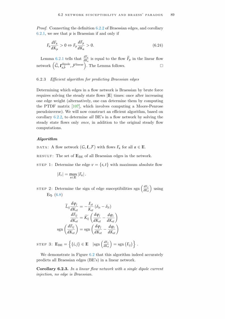
6.2 network susceptibility and braess’ paradox 89
Proof. Connecting the definition 6.2.2 of Braessian edges, and corollary
6.2.1, we see that µ is Braessian if and only if
FαdFα
dKµ> 0⇔ Fµ
dFµ
dKα> 0. (6.24)
Lemma 6.2.1 tells thatdFµ
dKαis equal to the flow Fµ in the linear flow
network(
G, Idipolea,b ,F linear)
. The Lemma follows.
6.2.3 Efficient algorithm for predicting Braessian edges
Determining which edges in a flow network is Braessian by brute force
requires solving the steady state flows |E| times: once after increasing
one edge weight (alternatively, one can determine them by computing
the PTDF matrix [107], which involves computing a Moore-Penrose
pseudoinverse). We will now construct an efficient algorithm, based on
corollary 6.2.2, to determine all BE’s in a flow network by solving the
steady state flows only once, in addition to the original steady flow
computations.
Algorithm
data: A flow network (G, I,F ) with flows Fα for all α ∈ E.
result: The set of EBE of all Braessian edges in the network.
step 1: Determine the edge ν = s, t with maximum absolute flow
|Fν| = maxα∈E|Fα| .
step 2: Determine the sign of edge susceptibilities sgn(
dFijdKst
)using
Eq. (6.8)
Lijdϕj
dKst= − Fst
Kst(δis − δit)
dFij
dKst= Kij
(dϕj
dKst− dϕi
dKst
)sgn
(dFij
dKst
)= sgn
(dϕj
dKst− dϕi
dKst
)
step 3: EBE =i, j ∈ E |sgn
(dFijdKst
)= sgn
(Fij)
.
We demonstrate in Figure 6.2 that this algorithm indeed accurately
predicts all Braessian edges (BE’s) in a linear network.
Corollary 6.2.3. In a linear flow network with a single dipole current
injection, no edge is Braessian.

90 braess’ paradox in continuous flow networks
−0.10 −0.05 0.00 0.05 0.10
FνdFνdKµ
−0.10
−0.05
0.00
0.05
0.10
c µνFµdFµ
dKν
Braessian
non-Braessian
y=x
0 50 100 150 200 250 300 350
Number of edges
10−2
10−1
100
101
102
Com
puta
tion
tim
e(s
econ
d)
indirect
direct
Figure 6.2: (left) Determining Braessian edges in a linear flow network by com-
puting FνdFνdKµ
by the efficient way Eq. (6.10) yields results identical
to the brute force calculations. ν is the most heavily loaded edge.
The x-axis shows direct computation and the y-axis the indirect
one. Blue dots represent Braessian edges, green dots non-Braessian
ones. Computation done on a 10× 10 square lattice network, with
25 randomly chosen sources and 25 randomly chosen sinks. (right)
The indirect method for computing Braessian edges is much faster
than the direct brute force method. For each network size, 10 in-
dependent runs were made. Error bars depict standard deviations.
Proof. Suppose the current inputs are +I and −I at nodes s and trespectively, and zero otherwise. Then the steady state flows are given
by Eq. (6.8),
Lij ϕj = I (δis − δit)
Fij = Kij(
ϕj − ϕi)
.(6.25)
The maximum flow, obviously, will be along the edge s, t. Now,
Lijdϕj
dKst= − Fst
Kst(δis − δit)
dFij
dKst= Kij
(dϕj
dKst− dϕi
dKst
)= − Kij
Kij
Fst
KstFij
⇒ FijdFij
dKst≥ 0
⇒ FstdFst
dKij≥ 0 (using corollary 6.2.1) .
(6.26)
Comparing Eq. (6.26) with definition 6.2.2, the corollary follows.
6.3 topological features behind braess’ paradox
So far, we have established that determining Braessian edges (BE’s)
on infinitesimally strengthening an edge in a conservative flow network
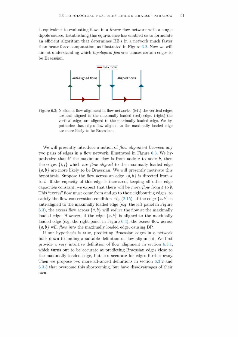
6.3 topological features behind braess’ paradox 91
is equivalent to evaluating flows in a linear flow network with a single
dipole source. Establishing this equivalence has enabled us to formulate
an efficient algorithm that determines BE’s in a network much faster
than brute force computation, as illustrated in Figure 6.2. Now we will
aim at understanding which topological features causes certain edges to
be Braessian.
Anti-aligned flows Aligned flows
Figure 6.3: Notion of flow alignment in flow networks. (left) the vertical edges
are anti-aligned to the maximally loaded (red) edge. (right) the
vertical edges are aligned to the maximally loaded edge. We hy-
pothesize that edges flow aligned to the maximally loaded edge
are more likely to be Braessian.
We will presently introduce a notion of flow alignment between any
two pairs of edges in a flow network, illustrated in Figure 6.3. We hy-
pothesize that if the maximum flow is from node a to node b, then
the edges i, j which are flow aligned to the maximally loaded edge
a, b are more likely to be Braessian. We will presently motivate this
hypothesis. Suppose the flow across an edge a, b is directed from ato b. If the capacity of this edge is increased, keeping all other edge
capacities constant, we expect that there will be more flow from a to b.
This “excess” flow must come from and go to the neighbouring edges, to
satisfy the flow conservation condition Eq. (2.15). If the edge a, b is
anti-aligned to the maximally loaded edge (e.g. the left panel in Figure
6.3), the excess flow across a, b will reduce the flow at the maximally
loaded edge. However, if the edge a, b is aligned to the maximally
loaded edge (e.g. the right panel in Figure 6.3), the excess flow across
a, b will flow into the maximally loaded edge, causing BP.
If our hypothesis is true, predicting Braessian edges in a network
boils down to finding a suitable definition of flow alignment. We first
provide a very intuitive definition of flow alignment in section 6.3.1,
which turns out to be accurate at predicting Braessian edges close to
the maximally loaded edge, but less accurate for edges further away.
Then we propose two more advanced definitions in section 6.3.2 and
6.3.3 that overcome this shortcoming, but have disadvantages of their
own.

92 braess’ paradox in continuous flow networks
6.3.1 Classifier based on edge distance
Definition 6.3.1 (Flow alignment by edge distance). Consider
a connected and simple flow network F = (G, I,F ). For each edge
e := i, j, let’s define i to be the “head” and j to be the “tail” if and
only if Fij > 0. Let d(s, t) be the shortest path length between nodes sand t. Label the edge set so that for all edges i, j, Fij > 0.
Then h1, t1 is defined to be aligned to the edge h2, t2
h1, t1⇒ h2, t2 (6.27)
if
mind(h1, t2), d(t1, h2) < mind(h1, h2), d(t1, t2). (6.28)
Likewise, h1, t1 is defined to be anti-aligned to the edge h2, t2
h1, t1 h2, t2 (6.29)
if
mind(h1, t2), d(t1, h2) > mind(h1, h2), d(t1, t2). (6.30)
We illustrate this definition in Figure 6.4.
We note that given two edges, one might neither be aligned nor be
anti-aligned, according to this definition.
Figure 6.4: Aligned and non-aligned flows, as defined in definition 6.3.1. e2 and
e3 are respectively aligned and anti-aligned to e1. Flow alignment
is undefined between e4 and e1.
Claim 6.3.1. If an edge i, j is aligned to the edge s, t with max-
imum flow in a network, then i, j is more likely to be a BE. If it is
anti-aligned, then it is less likely to be a BE.
We show the effectiveness of this classifier in Figure 6.5 in two net-
work topologies: a 30× 30 square lattice, and Voronoi tessellation of 20uniformly randomly drawn points from a unit square. In both topolo-
gies, 1/4th of the nodes were chosen to have inputs 1 and an equal

6.3 topological features behind braess’ paradox 93
0.0
0.2
0.4
0.6
0.8
1.0
frac
tion
ofed
ges
correct predictions false predictions can’t say
Distance01all
Edge distance based classifier on a 30x30 square lattice
BE, align
ed
notBE, an
ti-ali
gned
BE, anti-
align
ed
notBE, ali
gned
noeff
ect,
undefined
BE, undefined
notBE, undefi
ned
noeff
ect,
align
ed
noeff
ect,
anti-
align
ed0.0
0.2
0.4
0.6
0.8
1.0
frac
tion
ofed
ges
correct predictions false predictions can’t say
Distance01all
Edge distance based classifier on Voronoi tesselation of 20 points
Figure 6.5: The flow alignment based classifier as per claim 6.3.1 works well
for edges close to the edge with maximum flow, but worsens with
distance. Classifier was tested in two network topologies: 15× 15square lattice and Voronoi tessellation of 20 uniformly randomly
chosen points in the unit square. In each case 200 independent
runs were made. Error bars display the standard deviations. Edges
with susceptibilities ≤ 10−5 were assumed to have no effect on the
maximally loaded edge.

94 braess’ paradox in continuous flow networks
number to have inputs −1. The rest of the nodes had inputs 0. In both
topologies, 200 independent realizations were made. The edges with
ηµ→α < ε = 10−5, (6.31)
we considered to have too little effect on the maximally loaded edge
α to be called wither BE or not BE. We clearly see that for edges
with distance < 2 from the maximally loaded edge, the classifier is
quite accurate: there are very few edges that are not aligned, yet BE or
aligned, yet not BE. The accuracy of this predictor worsens, however,
for edges with distance ≥ 2 from the maximally loaded edge.
6.3.1.1 Reason behind false predictions in Topological classifier
We have seen that the edge distance based classifier fails for a significant
fraction of edges. Now we investigate for which edges this classifier fails.
In Figure 6.6, we illustrate the edges for which the classifier fails in a
Edge distance based classifier on a lattice
False predictionsmaxflow edge
Flows due to a dipole
Aligned flowsmaxflow edge
Figure 6.6: (left) Illustrating which edges are falsely classified by the edge
distance based classifier (we set the threshold ε as per Eq. (6.31) to
0). A region centered around the maximally loaded edge is shown.
(right) In purely dipole flows, the same edges happen to be aligned
with the dipole.
square lattice network. We see that these edges have one property in
common: they have aligned flows due to a purely dipole source term.
Lemma 6.2.1 then explains why our classifier fails at those edges. Only
those edges are Braessian, whose flows are in the same direction as
the flow would have been, if all the inputs were set to zero and a
single dipole were placed across the maximally loaded edge. The flow
alignment based classifier assumes the wrong direction to this dipole
flow on those edges, and consequently wrongly predicts Braessian edges.
6.3.2 Classifier based on cycle distance
Now that we know why our classifier performed poorly at certain edges,
we can build a better one by defining another way of computing align-

6.3 topological features behind braess’ paradox 95
ment of flows, according to which flows due to a single dipole are more
likely to be anti-aligned. Now we will present one such way of comput-
ing alignments of flows by replacing edge distances in definition 6.3.1 by
a certain “cycle distance”. In order to do that, we must define a couple
of graph theoretic quantities.
Figure 6.7: A planar graph (solid edges) and its dual (dashed edges, filled
circular nodes) corresponding to this specific embedding.
Definition 6.3.2. Dual graph
Given a planar graph G(V, E) and an embedding, we choose a cycle
basis BC consisting of the faces of the embedding. The dual graph GD is
a undirected multigraph whose vertex set is equal to BC. Its edge set E′
is as follows. For each edge e ∈ E, if it is shared between two cycles c1
and c2, then an edge between c and c′ is added to E′. We illustrate this
definition in Figure 6.7.
Definition 6.3.3 (Cycle distance). Given two cycles c1 and c2 in the
cycle basis BC of a graph G, the cycle distance between them dcycle (c1, c2)is simply the shortest path length in the dual graph between the nodes
c1 and c2.
Figure 6.8: Defining alignment of flows, according to cycle distance. The cycles
C+1/2 are flow-oriented to the flows in edges e1/2, and cycles C+
1/2are anti flow-oriented to the flows in edges e1/2. As a result, e1 and
e2 are flow aligned by cycle distance, because C+2 and C+
1 are only
one hop away, less than all other pairs.
Definition 6.3.4 (Flow-cycle alignment). Consider a connected,
simple, planar flow network F = (G, I,F ) in a specific plane embedding.

96 braess’ paradox in continuous flow networks
Let GD be the dual graph for this embedding. For each edge e := i, j,let’s define i to be the “head” and j to be the “tail” when Fij > 0. The edge
e is defined to be flow oriented to a cycle c containing e if the cycle,
when traversed in the anti-clockwise direction, encounters i before j.Otherwise, e is said to be anti flow-oriented to c.
Definition 6.3.5 (Flow alignment by cycle distance). Consider
a connected, simple, planar flow network F = (G, I,F ) in a specific
plane embedding and let GD be the dual graph for this embedding. For
each edge e, denote the cycle (if it exists) it is flow aligned to by C+e
and the cycle (if it exists) it is anti flow-oriented to by C−e .
Then two edges e1 and e2 are said to be aligned(anti-aligned) by cycle
distance if and only if
mindcycle(C+
1 , C+2)
, dcycle(C−1 , C−2
)
≷ mindcycle(C+
1 , C−2)
, dcycle(C−1 , C+
2). (6.32)
If either C+j or C−j does not exist, then all terms in the min function
containing it is omitted. If both C+j and C−j does not exist, flow align-
ment by cycle distance between them is undefined. We illustrate this
definition in Figure 6.8.
We evaluate the performance of this cycle-distance based classifier in
Figure 6.9, again in two topologies: square lattice and Voronoi tessel-
lations of uniformly randomly drawn points in R2, for the same flow
network realizations we tested the edge distance based classifier at (see
Figure 6.5). We see that for this classifier, the robustness of the classifi-
cation does not drop as much with distance as the edge distance based
classifier did. However, for Voronoi planar graphs, it fails to classify
more number of edges than the edge distance based one.
A crucial disadvantage of the cycle distance based classifier is that
it is applicable only to planar graphs. This is so because the notion of
flow cycle alignment in definition 6.3.4 cannot be defined for non-planar
graphs. We will now discuss yet another classifier, which overcomes
this restriction, at the same time being no less accurate than the cycle
distance based classifier for plane networks.
6.3.3 Flow rerouting classifier
Definition 6.3.6 (Rerouting alignment). Given a flow network
(G(V, E), I,F ), consider two edges e1 := s, t and e2 := m, n. As-
sume without loss of generality that Fst > 0, Fmn > 0. Then e2 is defined
to be aligned(anti-aligned) by flow rerouting to e1 if and only if in the
shortest simple path from s to t not containing s, t but containing
m, n, m appears before(after) n. This is illustrated in Figure 6.10.
We evaluate the performance of this flow rerouting based classifier
in Figure 6.11, the networks being identical to the ones considered for
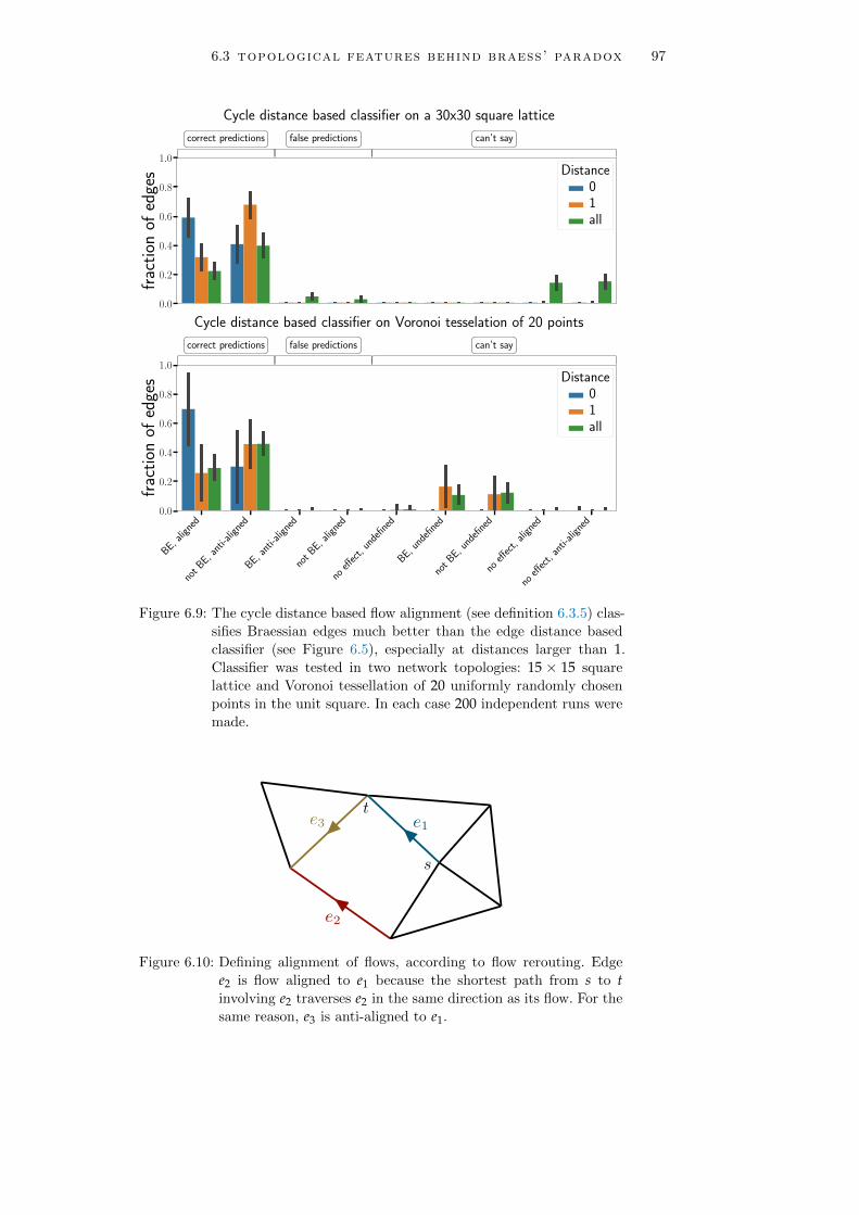
6.3 topological features behind braess’ paradox 97
0.0
0.2
0.4
0.6
0.8
1.0fr
acti
onof
edge
scorrect predictions false predictions can’t say
Distance01all
Cycle distance based classifier on a 30x30 square lattice
BE, align
ed
notBE, an
ti-ali
gned
BE, anti-
align
ed
notBE, ali
gned
noeff
ect,
undefined
BE, undefined
notBE, undefi
ned
noeff
ect,
align
ed
noeff
ect,
anti-
align
ed0.0
0.2
0.4
0.6
0.8
1.0
frac
tion
ofed
ges
correct predictions false predictions can’t say
Distance01all
Cycle distance based classifier on Voronoi tesselation of 20 points
Figure 6.9: The cycle distance based flow alignment (see definition 6.3.5) clas-
sifies Braessian edges much better than the edge distance based
classifier (see Figure 6.5), especially at distances larger than 1.
Classifier was tested in two network topologies: 15 × 15 square
lattice and Voronoi tessellation of 20 uniformly randomly chosen
points in the unit square. In each case 200 independent runs were
made.
Figure 6.10: Defining alignment of flows, according to flow rerouting. Edge
e2 is flow aligned to e1 because the shortest path from s to tinvolving e2 traverses e2 in the same direction as its flow. For the
same reason, e3 is anti-aligned to e1.

98 braess’ paradox in continuous flow networks
0.0
0.2
0.4
0.6
0.8
1.0
frac
tion
ofed
ges
correct predictions false predictions can’t say
Distance01all
Flow rerouting based classifier on a 30x30 square lattice
BE, align
ed
notBE, an
ti-ali
gned
BE, anti-
align
ed
notBE, ali
gned
noeff
ect,
undefined
BE, undefined
notBE, undefi
ned
noeff
ect,
align
ed
noeff
ect,
anti-
align
ed0.0
0.2
0.4
0.6
0.8
1.0
frac
tion
ofed
ges
correct predictions false predictions can’t say
Distance01all
Flow rerouting based classifier on Voronoi tesselation of 20 points
Figure 6.11: Flow rerouting based alignment (see definition 6.3.6) classifies
Braessian edges better than both the edge distance based one and
the cycle distance based one. Classifier was tested in two network
topologies: 15× 15 square lattice and Voronoi tessellation of 20uniformly randomly chosen points in the unit square. In each case
200 independent runs were made.

6.3 topological features behind braess’ paradox 99
testing the other two classifiers in Figure 6.5 and Figure 6.9. We see
that this classifier performs better than the edge distance based one
in both lattice and Voronoi graph topologies. Compared to the cycle
distance based one, it performs equally well.
6.3.4 Comparison between classifiers
BE
notBE
noeff
ect
0.1898 0.0840 0.0000
0.1909 0.2380 0.0000
0.1497 0.1475 0.0000
Edge distance alignment
0.2241 0.0498 0.0000
0.0307 0.3983 0.0000
0.1441 0.1531 0.0000
Cycle distance alignment
0.2241 0.0498 0.0000
0.0307 0.3983 0.0000
0.1441 0.1531 0.0000
Rerouting alignment
30x30 square lattice
align
ed
anti-
align
ed
undefined
BE
notBE
noeff
ect
0.2961 0.0419 0.0646
0.0774 0.3841 0.1231
0.0045 0.0056 0.0026
Edge distance alignment
align
ed
anti-
align
ed
undefined
0.2915 0.0021 0.1091
0.0021 0.4578 0.1247
0.0015 0.0021 0.0092
Cycle distance alignment
align
ed
anti-
align
ed
undefined
0.3426 0.0267 0.0333
0.0233 0.5285 0.0329
0.0042 0.0060 0.0026
Rerouting alignment
Voronoi tesselation of 20 points
Figure 6.12: Comparison of accuracies of three classifiers in predicting Braes-
sian edges in two topologies, 15× 15 square lattice and Voronoi
tessellation of 20 uniformly randomly chosen points in the unit
square. In each case 200 independent runs were made.
In Figure 6.12, we illustrate comparative performances of all the
three classifiers in two different network topologies: square lattices and
Voronoi planar graphs. We observe that for lattice topology, the edge
distance classifier suffers from significant false predictions. The cycle
distance classifier and the rerouting classifier works equally well, with
very little false predictions.
For Voronoi tessellations, the performances are more even across clas-
sifiers. The edge distance based classifier fares almost on par with the
other two, however the cycle distance classifier and rerouting classifier
both perform slightly better still. The cycle distance based classifier
has slightly less false predictions than the rerouting based one, but it
fails to classify (due to alignment being undefined) more edges than the
rerouting based one.
6.3.5 Effect of distance on classifier accuracy
We have already seen in Figures 6.5, 6.9 and 6.11 that all three classi-
fiers work well for edges at distances < 2 from the maximally loaded
edge, and their accuracies decrease for edges that are further away. Now

100 braess’ paradox in continuous flow networks
0 5 10 15 20 25 30
Distance
0.0
0.2
0.4
0.6
0.8
1.0
Acc
urac
y
edge dist
cycle dist
0 10 20 30 40 50 60
Distance
0.0
0.2
0.4
0.6
0.8
1.0
edge dist
cycle dist
0.0
0.2
0.4
0.6
0.8
1.0
Edg
esno
tcl
assi
fied
(das
hed
lines
)
Figure 6.13: (solid lines) Classification accuracy = Number of correct predictionsnumber of all predicted edges
for edge and cycle distance based classifiers. Threshold ε = 10−5,
as before. Simulation done on (left) a 30× 30 square lattice, with
200 independent runs; and (right) Voronoi tessellations of 2000randomly chosen points, with 50 independent runs. Cycle dis-
tance is much better than edge distance in lattices, especially
at large distances. In Voronoi tessellations, both classifiers work
well, edge distance based one slightly more so. But the gap be-
tween them decreases with distance. (dashed lines) Fraction of
edges that cannot be classified. For lattice networks, close to 0for both classifiers. For Voronoi, cycle distance based one fails
to classify more edges than the edge distance based one, but the
gap decreases with distance. All error bands depict standard de-
viations.
we systematically study how accurate the classifiers are at identifying
Braessian edges at different distances from the maximally loaded edge.
For our simulations, we choose as before, two network topologies. As
an accuracy measure, we choose the probability of correct prediction
= Number of correct predictionsNumber of all predicted edges . Due to the high runtime of the flow rerout-
ing based classifier for large networks, we omitted it from this study.
We present our findings in Figure 6.13. In square lattice topology, the
cycle distance based classifier is seen to be vastly superior to the edge
distance based one: the accuracy of it, after a slight drop till distance
< 6, actually increases with distance afterwards. It remains better in
accuracy than the edge distance based one at all distances. The accu-
racy of the edge distance based one steadily decreases with distance.
The situation, however, is quite different for Voronoi planar graphs.
The cycle distance based classifier is slightly less accurate than the edge
distance based one for distances < 40, after which it gets better. Both
classifiers manage accuracy ≈ 0.8 at all distances. Unlike in square
lattices, both classifiers fail to predict certain fraction of edges due to
alignment being undefined. The fraction of such unclassified edges is
also higher for cycle distance classifier, but the gap steadily declines
with distance.
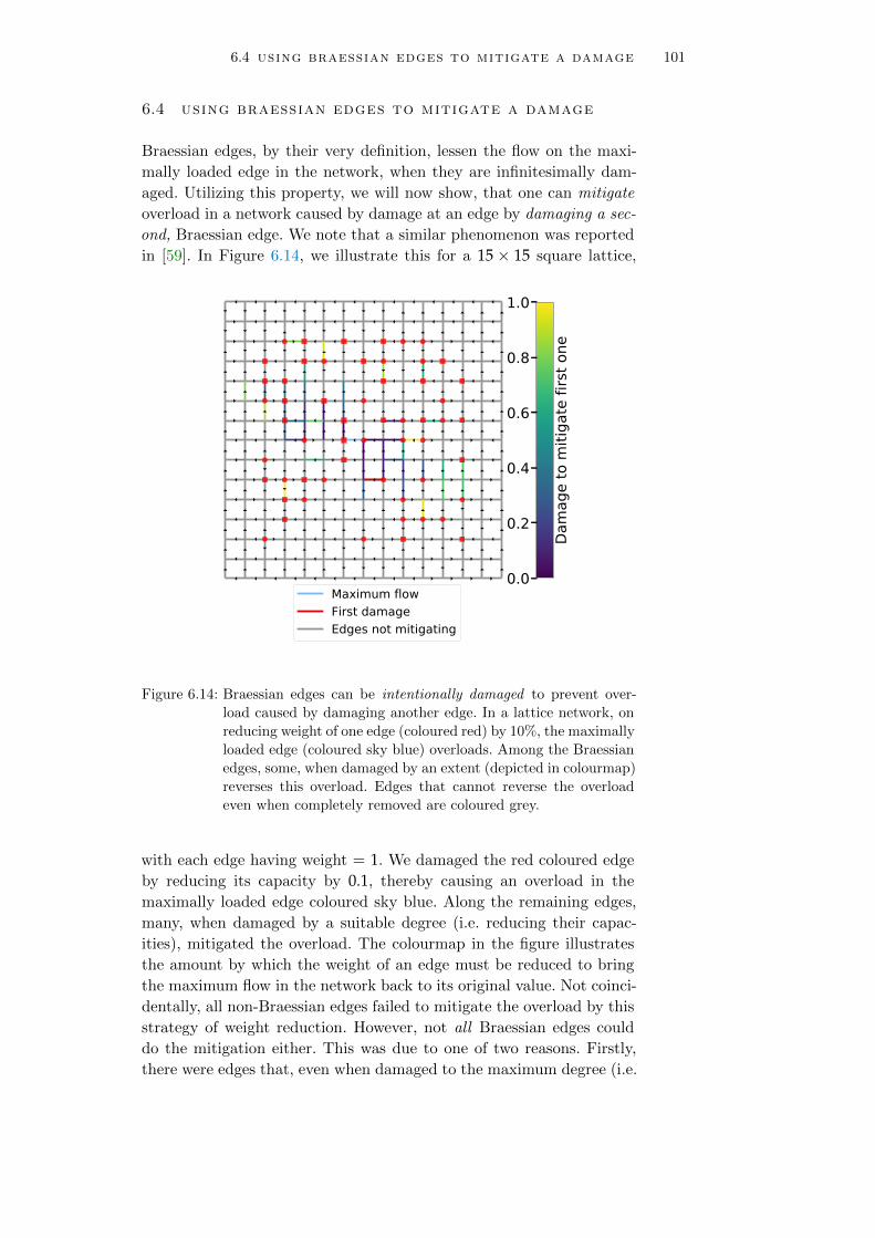
6.4 using braessian edges to mitigate a damage 101
6.4 using braessian edges to mitigate a damage
Braessian edges, by their very definition, lessen the flow on the maxi-
mally loaded edge in the network, when they are infinitesimally dam-
aged. Utilizing this property, we will now show, that one can mitigate
overload in a network caused by damage at an edge by damaging a sec-
ond, Braessian edge. We note that a similar phenomenon was reported
in [59]. In Figure 6.14, we illustrate this for a 15× 15 square lattice,
0.0
0.2
0.4
0.6
0.8
1.0
Dam
age
to m
itiga
te fi
rst o
ne
Maximum flowFirst damageEdges not mitigating
Figure 6.14: Braessian edges can be intentionally damaged to prevent over-
load caused by damaging another edge. In a lattice network, on
reducing weight of one edge (coloured red) by 10%, the maximally
loaded edge (coloured sky blue) overloads. Among the Braessian
edges, some, when damaged by an extent (depicted in colourmap)
reverses this overload. Edges that cannot reverse the overload
even when completely removed are coloured grey.
with each edge having weight = 1. We damaged the red coloured edge
by reducing its capacity by 0.1, thereby causing an overload in the
maximally loaded edge coloured sky blue. Along the remaining edges,
many, when damaged by a suitable degree (i.e. reducing their capac-
ities), mitigated the overload. The colourmap in the figure illustrates
the amount by which the weight of an edge must be reduced to bring
the maximum flow in the network back to its original value. Not coinci-
dentally, all non-Braessian edges failed to mitigate the overload by this
strategy of weight reduction. However, not all Braessian edges could
do the mitigation either. This was due to one of two reasons. Firstly,
there were edges that, even when damaged to the maximum degree (i.e.
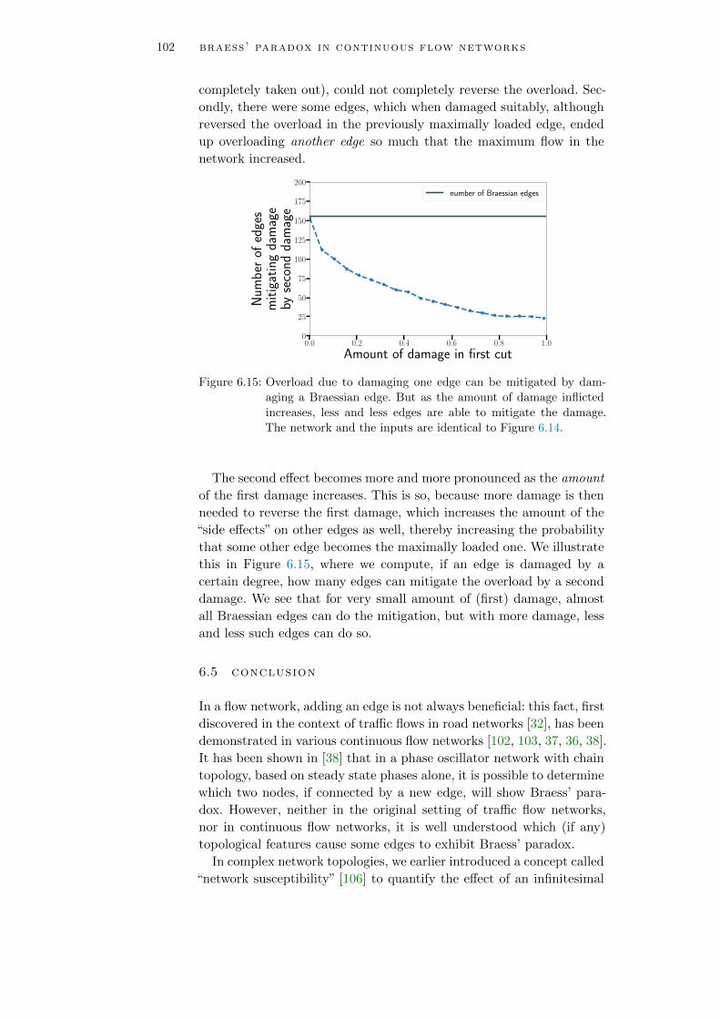
102 braess’ paradox in continuous flow networks
completely taken out), could not completely reverse the overload. Sec-
ondly, there were some edges, which when damaged suitably, although
reversed the overload in the previously maximally loaded edge, ended
up overloading another edge so much that the maximum flow in the
network increased.
0.0 0.2 0.4 0.6 0.8 1.0
Amount of damage in first cut
0
25
50
75
100
125
150
175
200
Num
ber
ofed
ges
mit
igat
ing
dam
age
byse
cond
dam
age
number of Braessian edges
Figure 6.15: Overload due to damaging one edge can be mitigated by dam-
aging a Braessian edge. But as the amount of damage inflicted
increases, less and less edges are able to mitigate the damage.
The network and the inputs are identical to Figure 6.14.
The second effect becomes more and more pronounced as the amount
of the first damage increases. This is so, because more damage is then
needed to reverse the first damage, which increases the amount of the
“side effects” on other edges as well, thereby increasing the probability
that some other edge becomes the maximally loaded one. We illustrate
this in Figure 6.15, where we compute, if an edge is damaged by a
certain degree, how many edges can mitigate the overload by a second
damage. We see that for very small amount of (first) damage, almost
all Braessian edges can do the mitigation, but with more damage, less
and less such edges can do so.
6.5 conclusion
In a flow network, adding an edge is not always beneficial: this fact, first
discovered in the context of traffic flows in road networks [32], has been
demonstrated in various continuous flow networks [102, 103, 37, 36, 38].
It has been shown in [38] that in a phase oscillator network with chain
topology, based on steady state phases alone, it is possible to determine
which two nodes, if connected by a new edge, will show Braess’ para-
dox. However, neither in the original setting of traffic flow networks,
nor in continuous flow networks, it is well understood which (if any)
topological features cause some edges to exhibit Braess’ paradox.
In complex network topologies, we earlier introduced a concept called
“network susceptibility” [106] to quantify the effect of an infinitesimal
6.5 conclusion 103
increase in an edge capacity on the flows in other edges. In this article,
we have used the tools of network susceptibility to study the question:
which edges in a network, when their capacities are infinitesimally in-
creased, cause an increase in the maximal load in the network? Under
a specific class of network dynamics, that we call conservative flow net-
works, we have shown that to answer to this question it is sufficient to
compute the flows in the same network due to a single dipole source
placed along the maximally loaded edge.
Utilizing this equivalence, we proceeded to define a topological notion
of flow alignment between two edges in a network and proposed that
such flow alignment will determine if an edge is Braessian. Our first
definition of flow alignment, based on edge distances, proved promising
but classified significant amount of edges wrongly as Braessian or non-
Braessian. We demonstrated that this classifier is improved significantly
if one replaces edge distances with cycle distances. However, our defini-
tion of cycle distance is not valid for non-planar networks. To overcome
this shortcoming, we defined yet another flow alignment, based on flow
reroutings, that works as well as the cycle distance based one for pre-
dicting Braessian edges, and is applicable for non-planar networks as
well.
We also showed that Braess’ paradox has a useful side effect: it is pos-
sible to mitigate the overload caused by damaging an edge by making
an additional damage at one of the Braessian edges.

A P P E N D I X
6.a moore-penrose pseudoinverse of symmetric ma-
trices
Lemma 6.A.1. If A is a symmetric matrix, then its Moore-Penrose
pseudoinverse A+ is also symmetric.
Proof. By definition, A+ is the unique Moore-Penrose pseudoinverse of
A if and only if
AA+ A = A (6.33)
A+ AA+ = A+ (6.34)
(AA+)T = AA+ (6.35)
(A+ A)T = A+ A (6.36)
Taking transpose of all these equations and exploiting A = AT yields:
A(
A+)T A = A (6.37)(
A+)T A
(A+)T
= A+ (6.38)
(A(
A+)T
)T = A(
A+)T
(6.39)
((
A+)T A)T =
(A+)T A. (6.40)
Therefore, AT is a valid Moore-Penrose pseudoinverse of A as well. By
uniqueness of A+, the lemma follows.

7F I N A L C O N C L U S I O N A N D O U T L O O K
In this thesis we have studied three different ways in which topology
influences the flows in a network: Firstly, which topological conditions
guarantee the stability of flows in phase oscillator networks; secondly,
which topological features result in more coexisting steady flows in the
same system; thirdly, which topological features cause certain edges in
a network to exhibit Braess paradox (i.e. the maximum flow in the
network increases when any of these edges are infinitesimally strength-
ened). In this Chapter we will summarize our key results, put them in
the context of existing research, and outline future research directions.
7.1 topology dependence of steady flows and their
stability
In Chapter 4, we studied how topology influences loss of stability in
a phase oscillator network whose dynamics follows the swing equation
(defined in Eq. (4.20)). This equation is frequently used to model the
high voltage AC power grid [19]. Loss of steady states in such systems
results in power outages, and hence establishing criteria for loss of sta-
bility in this system is an important problem.
We first derived an exact mapping between the fixed points and their
bifurcation structure of this model and that of the well studied Ku-
ramoto oscillators [1, 2]. It has been known for more than 40 years that
Kuramoto networks have a unique globally attracting steady state if the
coupling is stronger than a certain critical value, and no steady state
otherwise; for infinite and all-to-all coupled networks. But power grids
are far from all-to-all coupled: In fact, they are almost planar, with
very few long distance edges [20, 21]. For arbitrary topologies, neces-
sary and sufficient conditions for steady states in Kuramoto networks
are still not known.
One necessary condition for steady states (or steady flows) was pre-
sented using a purely graph theoretic approach in [45]: they considered
any cut or 2-partition of the network (i.e. a partition of the network
into two non-overlapping subnetworks, see Definition 2.1.5) and showed
that the power generated in one partition but not consumed there must
be able to flow to the other partition. This means coupling has to be
strong enough so that the edges in the cutset have enough capacity to
deliver this excess power. This leads to a necessary condition for the
existence of steady flows but not to a sufficient one, since steady states
in such networks must fulfill some geometric criteria [108] in addition
to the topological ones considered in this approach.
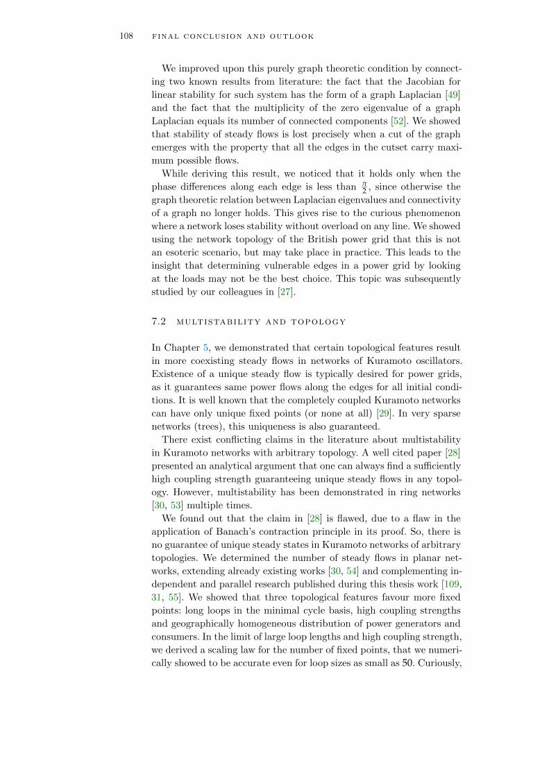
108 final conclusion and outlook
We improved upon this purely graph theoretic condition by connect-
ing two known results from literature: the fact that the Jacobian for
linear stability for such system has the form of a graph Laplacian [49]
and the fact that the multiplicity of the zero eigenvalue of a graph
Laplacian equals its number of connected components [52]. We showed
that stability of steady flows is lost precisely when a cut of the graph
emerges with the property that all the edges in the cutset carry maxi-
mum possible flows.
While deriving this result, we noticed that it holds only when the
phase differences along each edge is less than π2 , since otherwise the
graph theoretic relation between Laplacian eigenvalues and connectivity
of a graph no longer holds. This gives rise to the curious phenomenon
where a network loses stability without overload on any line. We showed
using the network topology of the British power grid that this is not
an esoteric scenario, but may take place in practice. This leads to the
insight that determining vulnerable edges in a power grid by looking
at the loads may not be the best choice. This topic was subsequently
studied by our colleagues in [27].
7.2 multistability and topology
In Chapter 5, we demonstrated that certain topological features result
in more coexisting steady flows in networks of Kuramoto oscillators.
Existence of a unique steady flow is typically desired for power grids,
as it guarantees same power flows along the edges for all initial condi-
tions. It is well known that the completely coupled Kuramoto networks
can have only unique fixed points (or none at all) [29]. In very sparse
networks (trees), this uniqueness is also guaranteed.
There exist conflicting claims in the literature about multistability
in Kuramoto networks with arbitrary topology. A well cited paper [28]
presented an analytical argument that one can always find a sufficiently
high coupling strength guaranteeing unique steady flows in any topol-
ogy. However, multistability has been demonstrated in ring networks
[30, 53] multiple times.
We found out that the claim in [28] is flawed, due to a flaw in the
application of Banach’s contraction principle in its proof. So, there is
no guarantee of unique steady states in Kuramoto networks of arbitrary
topologies. We determined the number of steady flows in planar net-
works, extending already existing works [30, 54] and complementing in-
dependent and parallel research published during this thesis work [109,
31, 55]. We showed that three topological features favour more fixed
points: long loops in the minimal cycle basis, high coupling strengths
and geographically homogeneous distribution of power generators and
consumers. In the limit of large loop lengths and high coupling strength,
we derived a scaling law for the number of fixed points, that we numeri-
cally showed to be accurate even for loop sizes as small as 50. Curiously,
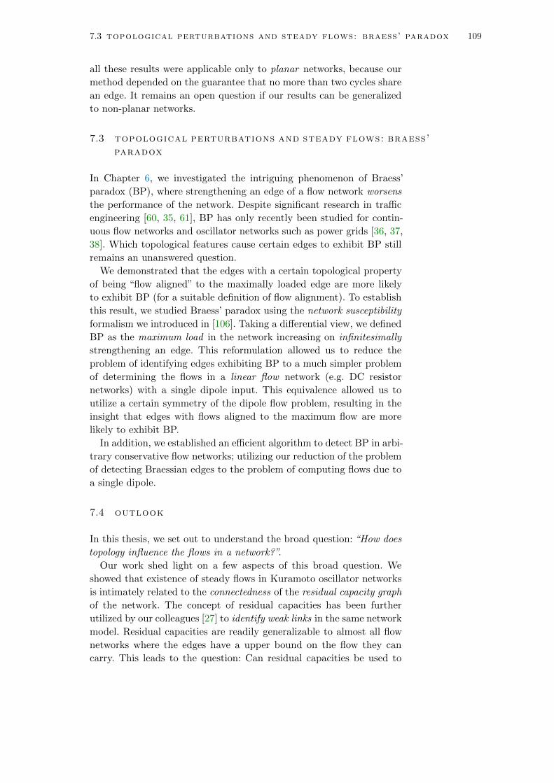
7.3 topological perturbations and steady flows: braess’ paradox 109
all these results were applicable only to planar networks, because our
method depended on the guarantee that no more than two cycles share
an edge. It remains an open question if our results can be generalized
to non-planar networks.
7.3 topological perturbations and steady flows: braess’
paradox
In Chapter 6, we investigated the intriguing phenomenon of Braess’
paradox (BP), where strengthening an edge of a flow network worsens
the performance of the network. Despite significant research in traffic
engineering [60, 35, 61], BP has only recently been studied for contin-
uous flow networks and oscillator networks such as power grids [36, 37,
38]. Which topological features cause certain edges to exhibit BP still
remains an unanswered question.
We demonstrated that the edges with a certain topological property
of being “flow aligned” to the maximally loaded edge are more likely
to exhibit BP (for a suitable definition of flow alignment). To establish
this result, we studied Braess’ paradox using the network susceptibility
formalism we introduced in [106]. Taking a differential view, we defined
BP as the maximum load in the network increasing on infinitesimally
strengthening an edge. This reformulation allowed us to reduce the
problem of identifying edges exhibiting BP to a much simpler problem
of determining the flows in a linear flow network (e.g. DC resistor
networks) with a single dipole input. This equivalence allowed us to
utilize a certain symmetry of the dipole flow problem, resulting in the
insight that edges with flows aligned to the maximum flow are more
likely to exhibit BP.
In addition, we established an efficient algorithm to detect BP in arbi-
trary conservative flow networks; utilizing our reduction of the problem
of detecting Braessian edges to the problem of computing flows due to
a single dipole.
7.4 outlook
In this thesis, we set out to understand the broad question: “How does
topology influence the flows in a network?”.
Our work shed light on a few aspects of this broad question. We
showed that existence of steady flows in Kuramoto oscillator networks
is intimately related to the connectedness of the residual capacity graph
of the network. The concept of residual capacities has been further
utilized by our colleagues [27] to identify weak links in the same network
model. Residual capacities are readily generalizable to almost all flow
networks where the edges have a upper bound on the flow they can
carry. This leads to the question: Can residual capacities be used to

110 final conclusion and outlook
understand dynamical properties of other flow networks as well (such
as the third order model of power grids [70])?
We found an answer to the puzzle of conflicting claims in the litera-
ture regarding uniqueness of steady flows in phase oscillator networks.
Building upon and extending existing knowledge [30, 31, 55] on the
number of coexisting steady flows, we demonstrated that the number
of steady flows increase with three topological features: cycle lengths,
edge capacities and input heterogeneities. Our findings indicate that
power grids may cease to have unique steady flows if the distribution
of generators and consumers get more decentral. This may be problem-
atic, since our power grids are gradually getting more decentral; due to
big coal and nuclear power plants being phased out in favour of smaller
and more distributed wind or solar power based generators to reduce
CO2 emissions [62]. In addition, decentral grids have been shown to be
more robust against topological perturbations [71]. Strategies to design
decentral power grids, while maintaining unique steady flows would be
interesting to study.
Knowing the number of steady flows in a network is important for
understanding its dynamics. The next question of interest is measuring
the basin volumes of those steady flows, i.e. answering “how likely is
the network to end up with one specific steady flow, if it is started
from many random initial conditions?”. This topic was first raised for
Kuramoto networks in [53], and aspects of it has been presented in a
recent preprint [110].
While we have made substantial progress into predicting which edges
cause Braess paradox in linear flow networks, it remains to be seen if
our works hold for nonlinear flow networks, e.g. models of AC power
grid. Analytical insights motivating our predictor of Braessian edges
remains valid for a broad class of nonlinear flow networks, including
the swing equation model of power grids.
in many real networks, it is more important to know whether Braess
paradox would occur on adding an edge, rather than on infinitesimally
strengthening an edge. We studied the second question because it was
analytically tractable by using edge-to-edge susceptibilities that we in-
troduced in [106]. However, we hope that our findings can be extended
to find out Braessian edges on adding an edge as well, because there ex-
ists a concept called “line outage distribution factor” (LODF) in power
engineering, that quantifies the flow changes in a network on complete
removal of an edge. LODF’s happen to be related to edge-to-edge sus-
ceptibilities by a prefactor [107].
Much remains to be answered of the question we posed at the begin-
ning of this thesis:“How does topology influence the flows in a network?”
This question will arise in additional contexts in future, as the tools of
network science are introduced to study new systems, e.g. the flow of
information in the world wide web, or the flow of cars in road networks.
While approaches specific to the system at hand are indispensable for

7.4 outlook 111
understanding them, a generalized approach of establishing causal rela-
tionships between topology and dynamics may give rise to new insights
by uncovering unifying features across different systems.

B I B L I O G R A P H Y
[1] Y. Kuramoto. “Self-entrainment of a population of coupled non-
linear oscillators.” In: International Symposium on on Mathe-
matical Problems in Theoretical Physics. Ed. by H. Araki. Lec-
ture Notes in Physics Vol. 39. New York: Springer, 1975, p. 420.
[2] Juan A Acebron et al.“The Kuramoto model: A simple paradigm
for synchronization phenomena.” In: Reviews of modern physics
77.1 (2005), p. 137.
[3] H. Hildenbrandt, C. Carere, and C.K. Hemelrijk.“Self-organized
aerial displays of thousands of starlings: a model.” In: Behavioral
Ecology 21.6 (2010), pp. 1349–1359.
[4] Steven H. Strogatz.“From Kuramoto to Crawford: Exploring the
onset of synchronization in populations of coupled oscillators.”
In: Physica D: Nonlinear Phenomena 143 (2000), p. 1.
[5] Jesus Gomez-Gardenes et al. “Explosive synchronization transi-
tions in scale-free networks.” In: Physical review letters 106.12
(2011), p. 128701.
[6] Fumiko Yonezawa, Shoichi Sakamoto, and Motoo Hori. “Percola-
tion in two-dimensional lattices. II. The extent of universality.”
In: Physical Review B 40.1 (1989), p. 650.
[7] Fumiko Yonezawa, Shoichi Sakamoto, and Motoo Hori. “Perco-
lation in two-dimensional lattices. I. A technique for the estima-
tion of thresholds.” In: Physical Review B 40.1 (1989), p. 636.
[8] Reinhard Diestel. Graph Theory (Graduate Texts in Mathemat-
ics). Springer, 2000. isbn: 0387989765.
[9] Donald E Knuth. “A generalization of Dijkstra’s algorithm.” In:
Information Processing Letters 6.1 (1977), pp. 1–5.
[10] Otakar Boruvka. “O jistem problemu minimalnım.” In: Prace
moravske prırodovedecke spolecnosti v Brne 111.3 (1926), pp. 37–
58.
[11] Duncan J Watts and Steven H Strogatz. “Collective dynamics of
‘small-world’networks.” In: nature 393.6684 (1998), pp. 440–442.
[12] A. L. Barabasi and R. Albert. “Emergence of scaling in random
networks.” In: science 286.5439 (1999), pp. 509–512.
[13] Carsten Matke et al. “Structure Analysis of the German Trans-
mission Network Using the Open Source Model SciGRID.” In:
(2017), pp. 177–188.
114 bibliography
[14] Eleni Katifori, Gergely J Szollosi, and Marcelo O Magnasco.
“Damage and fluctuations induce loops in optimal transport net-
works.” In: Physical Review Letters 104.4 (2010), p. 048704.
[15] Kurt Wiesenfeld, Pere Colet, and Steven H Strogatz. “Synchro-
nization transitions in a disordered Josephson series array.” In:
Physical review letters 76.3 (1996), p. 404.
[16] Francisco Varela et al. “The brainweb: phase synchronization
and large-scale integration.” In: Nature reviews neuroscience 2.4
(2001), pp. 229–239.
[17] Istvan Z Kiss, Yumei Zhai, and John L Hudson. “Emerging
coherence in a population of chemical oscillators.” In: Science
296.5573 (2002), pp. 1676–1678.
[18] Brian Stott, Jorge Jardim, and Ongun Alsac. “DC power flow
revisited.”In: IEEE Transactions on Power Systems 24.3 (2009),
pp. 1290–1300.
[19] Giovanni Filatrella, Arne Hejde Nielsen, and Niels Falsig Ped-
ersen. “Analysis of a power grid using a Kuramoto-like model.”
In: The European Physical Journal B - Condensed Matter and
Complex Systems 61.4 (2008), pp. 485–491.
[20] Saleh Soltan and Gil Zussman.“Generation of synthetic spatially
embedded power grid networks.” In: Power and Energy Society
General Meeting (PESGM), 2016. IEEE. 2016, pp. 1–5.
[21] Paul Schultz, Jobst Heitzig, and Jurgen Kurths. “A random
growth model for power grids and other spatially embedded in-
frastructure networks.” In: The European Physical Journal Spe-
cial Topics 223.12 (2014), pp. 2593–2610.
[22] Jesus Gomez-Gardenes, Yamir Moreno, and Alex Arenas. “Syn-
chronizability determined by coupling strengths and topology on
complex networks.”In: Physical Review E 75.6 (2007), p. 066106.
[23] Hyunsuk Hong, Moo-Young Choi, and Beom Jun Kim. “Syn-
chronization on small-world networks.” In: Physical Review E
65.2 (2002), p. 026139.
[24] Patrick N McGraw and Michael Menzinger. “Clustering and the
synchronization of oscillator networks.” In: Physical Review E
72.1 (2005), p. 015101.
[25] Motoki Nagata et al. “Smoothing effect for spatially distributed
renewable resources and its impact on power grid robustness.”
In: Chaos: An Interdisciplinary Journal of Nonlinear Science
27.3 (2017), p. 033104.
[26] Martin Rohden et al. “Self-organized synchronization in decen-
tralized power grids.” In: Physical review letters 109.6 (2012),
p. 064101.
bibliography 115
[27] Dirk Witthaut et al. “Critical links and nonlocal rerouting in
complex supply networks.” In: Physical review letters 116.13
(2016), p. 138701.
[28] Ali Jadbabaie, Nader Motee, and Mauricio Barahona. “On the
stability of the Kuramoto model of coupled nonlinear oscilla-
tors.” In: Proceedings of the 2004 American Control Conference.
Vol. 5. IEEE. 2004, pp. 4296–4301.
[29] Richard Taylor.“There is no non-zero stable fixed point for dense
networks in the homogeneous Kuramoto model.” In: Journal of
Physics A: Mathematical and Theoretical 45.5 (2012), p. 055102.
[30] J Ochab and PF Gora. “Synchronization of coupled oscillators
in a local one-dimensional Kuramoto model.” In: Acta Physica
Polonica. Series B, Proceedings Supplement 3.2 (2010), pp. 453–
462.
[31] Robin Delabays, Tommaso Coletta, and Philippe Jacquod.“Mul-
tistability of phase-locking and topological winding numbers in
locally coupled Kuramoto models on single-loop networks.” In:
Journal of Mathematical Physics 57.3 (2016), p. 032701.
[32] Dietrich Braess. “Uber ein Paradoxon aus der Verkehrsplanung.”
In: Unternehmensforschung 12.1 (1968), pp. 258–268.
[33] Richard Steinberg and Willard I. Zangwill. “The Prevalence of
Braess’ Paradox.”In: Transportation Science 17.3 (1983), pp. 301–
318.
[34] Stella Dafermos and Anna Nagurney. “On some traffic equilib-
rium theory paradoxes.” In: Transportation Research Part B:
Methodological 18.2 (1984), pp. 101–110.
[35] Eric I. Pas and Shari L. Principio. “Braess’ paradox: Some new
insights.” In: Transportation Research Part B: Methodological
31.3 (1997), pp. 265–276.
[36] Dirk Witthaut and Marc Timme. “Braess’s paradox in oscillator
networks, desynchronization and power outage.”In: New journal
of physics 14.8 (2012), p. 083036.
[37] Dirk Witthaut and Marc Timme. “Nonlocal failures in complex
supply networks by single link additions.” In: The European
Physical Journal B 86.9 (2013), p. 377.
[38] Tommaso Coletta and Philippe Jacquod. “Linear stability and
the Braess paradox in coupled-oscillator networks and electric
power grids.” In: Physical Review E 93.3 (2016), p. 032222.
[39] Chris Godsil and Gordon F Royle. Algebraic graph theory. Vol. 207.
Springer Science & Business Media, 2013.
[40] Alex Arenas et al. “Synchronization in complex networks.” In:
Physics reports 469.3 (2008), pp. 93–153.

116 bibliography
[41] Dirk Witthaut and Marc Timme.“Kuramoto dynamics in Hamil-
tonian systems.” In: Physical Review E 90.3 (2014), p. 032917.
[42] Marc Durand. “Structure of optimal transport networks subject
to a global constraint.” In: Physical Review Letters 98.8 (2007),
p. 088701.
[43] Dean Karnopp. Bond graph models for fluid dynamic systems.
American Society of Mechanical Engineers, 1972.
[44] Clayton R Paul. Fundamentals of electric circuit analysis. Wiley,
2001.
[45] Sergi Lozano, Lubos Buzna, and Albert Dıaz-Guilera. “Role of
network topology in the synchronization of power systems.” In:
The European Physical Journal B-Condensed Matter and Com-
plex Systems 85.7 (2012), pp. 1–8.
[46] Mauricio Barahona and Louis M Pecora. “Synchronization in
small-world systems.” In: Physical review letters 89.5 (2002),
p. 054101.
[47] Nikhil Chopra and Mark W Spong. “On synchronization of Ku-
ramoto oscillators.” In: Decision and Control, 2005 and 2005
European Control Conference. CDC-ECC’05. 44th IEEE Con-
ference on. IEEE. 2005, pp. 3916–3922.
[48] Alexander C Kalloniatis. “From incoherence to synchronicity
in the network Kuramoto model.” In: Physical Review E 82.6
(2010), p. 066202.
[49] Florian Dorfler, Michael Chertkov, and Francesco Bullo. “Syn-
chronization in complex oscillator networks and smart grids.” In:
Proceedings of the National Academy of Sciences 110.6 (2013),
pp. 2005–2010.
[50] Per Sebastian Skardal, Dane Taylor, and Jie Sun. “Optimal syn-
chronization of complex networks.” In: Physical review letters
113.14 (2014), p. 144101.
[51] Florian Dorfler and Francesco Bullo. “Synchronization in com-
plex networks of phase oscillators: A survey.” In: Automatica
50.6 (2014), pp. 1539–1564.
[52] M. E. J. Newman. Networks – An introduction. Oxford: Oxford
University Press, 2010. isbn: 978-0-19-920665-0.
[53] Daniel A Wiley, Steven H Strogatz, and Michelle Girvan. “The
size of the sync basin.” In: Chaos: An Interdisciplinary Journal
of Nonlinear Science 16.1 (2006), p. 015103.
[54] Dhagash Mehta et al.“Algebraic geometrization of the Kuramoto
model: Equilibria and stability analysis.” In: Chaos: An Interdis-
ciplinary Journal of Nonlinear Science 25.5 (2015), p. 053103.

bibliography 117
[55] Robin Delabays, Tommaso Coletta, and Philippe Jacquod.“Mul-
tistability of phase-locking in equal-frequency Kuramoto models
on planar graphs.” In: Journal of Mathematical Physics 58.3
(2017), p. 032703.
[56] U.S.-Canada Power System Outage Task Force. https://reports.
energy.gov/BlackoutFinal-Web.pdf. 2004.
[57] Union for the Coordination of Transmission of Electricity. Final
report on the system disturbance on 4 November 2006. http://
www.entsoe.eu/~library/publications/ce/otherreports/
Final-Report-20070130.pdf. 2007.
[58] Ake J Holmgren. “Using graph models to analyze the vulnera-
bility of electric power networks.” In: Risk analysis 26.4 (2006),
pp. 955–969.
[59] Adilson E Motter. “Cascade control and defense in complex net-
works.” In: Physical Review Letters 93.9 (2004), p. 098701.
[60] Marguerite Frank. “The Braess paradox.” In: Mathematical Pro-
gramming 20.1 (1981), pp. 283–302.
[61] Gregory Valiant and Tim Roughgarden. “Braess’s Paradox in
large random graphs.” In: Random Structures & Algorithms 37.4
(2010), pp. 495–515.
[62] Emma Marris. “Energy: Upgrading the grid.” In: Nature News
454.7204 (2008), pp. 570–573.
[63] John A Turner. “A realizable renewable energy future.” In: Sci-
ence 285.5428 (1999), pp. 687–689.
[64] Thiemo Pesch, H-J Allelein, and J-F Hake.“Impacts of the trans-
formation of the German energy system on the transmission
grid.” In: The European Physical Journal Special Topics 223.12
(2014), pp. 2561–2575.
[65] Dominik Heide et al. “Seasonal optimal mix of wind and solar
power in a future, highly renewable Europe.” In: Renewable En-
ergy 35.11 (2010), pp. 2483–2489.
[66] Frank Bottcher, Joachim Peinke, et al. “Small and large scale
fluctuations in atmospheric wind speeds.” In: Stochastic envi-
ronmental research and risk assessment 21.3 (2007), pp. 299–
308.
[67] Patrick Milan, Matthias Wachter, and Joachim Peinke. “Turbu-
lent character of wind energy.” In: Physical review letters 110.13
(2013), p. 138701.
[68] Arthur R Bergen and David J Hill. “A structure preserving
model for power system stability analysis.” In: IEEE Transac-
tions on Power Apparatus and Systems 1 (1981), pp. 25–35.

118 bibliography
[69] David J Hill and Guanrong Chen. “Power systems as dynamic
networks.” In: Circuits and Systems, 2006. ISCAS 2006. Pro-
ceedings. 2006 IEEE International Symposium on. IEEE. 2006,
4–pp.
[70] Jan Machowski, Janusz W Bialek, and James Richard Bumby.
Power system dynamics, stability and control. New York: John
Wiley & Sons, 2008.
[71] Martin Rohden et al. “Impact of network topology on synchrony
of oscillatory power grids.” In: Chaos: An Interdisciplinary Jour-
nal of Nonlinear Science 24.1 (2014), p. 013123.
[72] Adilson E Motter et al. “Spontaneous synchrony in power-grid
networks.” In: Nature Physics 9.3 (2013), pp. 191–197.
[73] Peter J Menck et al. “How dead ends undermine power grid
stability.” In: Nature communications 5 (2014).
[74] Prabha Kundur, Neal J Balu, and Mark G Lauby. Power system
stability and control. Vol. 7. McGraw-hill New York, 1994.
[75] Yoshihiko Susuki, Igor Mezic, and Takashi Hikihara. “Global
swing instability of multimachine power systems.” In: Decision
and Control, 2008. CDC 2008. 47th IEEE Conference on. IEEE.
2008, pp. 2487–2492.
[76] Yoshihiko Susuki, Igor Mezic, and Takashi Hikihara. “Coherent
swing instability of power grids.”In: Journal of nonlinear science
21.3 (2011), pp. 403–439.
[77] Florian Dorfler and Francesco Bullo. “Kron reduction of graphs
with applications to electrical networks.” In: IEEE Transactions
on Circuits and Systems I: Regular Papers 60.1 (2013), pp. 150–
163.
[78] Katrin Schmietendorf et al. “Self-organized synchronization and
voltage stability in networks of synchronous machines.” In: The
European Physical Journal Special Topics 223.12 (2014), pp. 2577–
2592.
[79] Hsiao-Dong Chiang, Felix Wu, and P Varaiya. “Foundations of
direct methods for power system transient stability analysis.”
In: IEEE Transactions on Circuits and systems 34.2 (1987),
pp. 160–173.
[80] CJ Perez and F Ritort. “A moment-based approach to the dy-
namical solution of the Kuramoto model.” In: Journal of Physics
A: Mathematical and General 30.23 (1997), p. 8095.
[81] James Howard. “Stability of Hamiltonian equilibria.” In: Schol-
arpedia 8 (2013), p. 3627. doi: 10.4249/scholarpedia.3627.
[82] Hassan K Khalil and JW Grizzle. Nonlinear systems. Vol. 3.
Prentice hall Upper Saddle River, 2002.

bibliography 119
[83] M Levi, Frank C Hoppensteadt, and WL Miranker. “Dynamics
of the Josephson junction.” In: Quarterly of Applied Mathemat-
ics 36.2 (1978), pp. 167–198.
[84] Hannes Risken. Fokker-planck equation. Springer, 1996, pp. 63–
95.
[85] Peter J Menck et al.“How basin stability complements the linear-
stability paradigm.” In: Nature Physics 9.2 (2013), pp. 89–92.
[86] Yuri A Kuznetsov. Elements of applied bifurcation theory. Vol. 112.
Springer Science & Business Media, 2013.
[87] Patrick C Parks. “AM Lyapunov’s stability theory - 100 years
on.” In: IMA journal of Mathematical Control and Information
9.4 (1992), pp. 275–303.
[88] Union for the Coordination of Transmission of Electricity. Con-
tinental Europe Operation Handbook. https://www.entsoe.
eu/publications/system-operations-reports/operation-
handbook/Pages/default.aspx. 2014.
[89] Peter Fairley. “The unruly power grid.” In: IEEE Spectrum 41.8
(2004), pp. 22–27.
[90] Ingve Simonsen et al. “Transient dynamics increasing network
vulnerability to cascading failures.” In: Physical review letters
100.21 (2008), p. 218701.
[91] William N Anderson Jr and Thomas D Morley. “Eigenvalues of
the Laplacian of a graph.” In: Linear and multilinear algebra
18.2 (1985), pp. 141–145.
[92] Bojan Mohar et al. “The Laplacian spectrum of graphs.” In:
Graph theory, combinatorics, and applications 2.871-898 (1991),
p. 12.
[93] Miroslav Fiedler.“Algebraic connectivity of graphs.”In: Czechoslo-
vak mathematical journal 23.2 (1973), pp. 298–305.
[94] Santo Fortunato. “Community detection in graphs.” In: Physics
reports 486.3 (2010), pp. 75–174.
[95] Surya D Pathak et al. “Complexity and adaptivity in supply net-
works: Building supply network theory using a complex adaptive
systems perspective.” In: Decision sciences 38.4 (2007), pp. 547–
580.
[96] Antonio MT Ramos and Carmen PC Prado. “Role of hystere-
sis in stomatal aperture dynamics.” In: Physical Review E 87.1
(2013), p. 012719.
[97] Kare Hartvig Jensen et al. “Optimality of the Munch mechanism
for translocation of sugars in plants.” In: Journal of the Royal
Society Interface 8.61 (2011), pp. 1155–1165.
120 bibliography
[98] JW Patrick. “Phloem unloading: sieve element unloading and
post-sieve element transport.” In: Annual review of plant biology
48.1 (1997), pp. 191–222.
[99] Yannis A. Korilis, Aurel A. Lazar, and Ariel Orda. “Avoiding
the Braess paradox in non-cooperative networks.” In: Journal
of Applied Probability 36.1 (1999), pp. 211–222.
[100] R.E. Azouzi, E. Altman, and O. Pourtallier. “Properties of equi-
libria in competitive routing with several user types.” In: vol. 4.
IEEE, 2002, pp. 3646–3651.
[101] Rinaldo M. Colombo and Helge Holden.“On the Braess Paradox
with Nonlinear Dynamics and Control Theory.” In: Journal of
Optimization Theory and Applications 168.1 (2016), pp. 216–
230.
[102] Joel E. Cohen and Paul Horowitz. “Paradoxical behaviour of
mechanical and electrical networks.” In: Nature 352.6337 (1991),
pp. 699–701.
[103] Ladimer S Nagurney and Anna Nagurney.“Physical proof of the
occurrence of the Braess Paradox in electrical circuits.” In: EPL
(Europhysics Letters) 115.2 (2016), p. 28004.
[104] S Toussaint et al. “Counterintuitive behavior of simulated net-
work’s conductance analogous to the Braess paradox.” In: Bul-
letin of the American Physical Society 61 (2016).
[105] Ian Dobson et al. “Complex systems analysis of series of black-
outs: Cascading failure, critical points, and self-organization.”In:
Chaos: An Interdisciplinary Journal of Nonlinear Science 17.2
(2007), p. 026103.
[106] Debsankha Manik et al. “Network susceptibilities: Theory and
applications.” In: Physical Review E 95.1 (2017), p. 012319.
[107] Henrik Ronellenfitsch et al. “Dual theory of transmission line
outages.” In: IEEE Transactions on Power Systems (2017).
[108] Debsankha Manik et al. “Supply networks: Instabilities with-
out overload.” In: The European Physical Journal Special Topics
223.12 (2014), pp. 2527–2547.
[109] Kaihua Xi, Johan LA Dubbeldam, and Hai Xiang Lin. “Syn-
chronization of cyclic power grids: Equilibria and stability of
the synchronous state.” In: Chaos: An Interdisciplinary Journal
of Nonlinear Science 27.1 (2017), p. 013109.
[110] Robin Delabays, Melvyn Tyloo, and Philippe Jacquod.“The Size
of the Sync Basin Revisited.”In: arXiv preprint arXiv:1706.00344
(2017).

AC K N OW L E D G M E N T S
Firstly, I would like to thank Marc: for letting me dabble in all those
network related projects: powergrids, ecobus, law evolution, and more.
Some of them produced less scientific results then others, but you were
never anything but encouraging. I learnt something from each of these
projects, and am happy that I tried.
I would like to thank Dirk (my unofficial co-supervisor): I never cease
to be amazed at how effortlessly you converted ideas and notes coming
from brainstorming sessions into working drafts of manuscripts.
Thank you Eleni, for introducing me to networks in biological sys-
tems, and showing that one can have fun with cool mathematical tools,
and at the same time understand real stuff in nature.
Thank you Andreas, Harold, Jana, Tariq, Sebastian, Alexander and
everybody in the Python teaching gang: due to you, I never stopped
learning programming and other computer related stuff, and it made
my PhD so much more fun.
Special thanks go to Nora, Tariq, and Andreas, for proofreading my
thesis and giving me so many constructive criticisms.
Warm thanks to everybody in the network dynamics group, and the
rest of you in the now gone Bunsenstrasse building, for leaving me
with so many fond memories of my PhD life: coffee breaks at the red
kitchen, cooking evenings at the yellow kitchen, barbecue on the terrace
in summer, one day trips, ruthless grilling at the test talks and so much
more.
I thank the whole CoNDyNet crowd: Martin, Frank, Sabine, Paul,
Carsten, Tom (and the rest) for the amazing time at all the conferences.
I thank my family in India, for always being supportive, and trusting
that I knew what I was doing. Last but not the least, thank you Fenna:
for making sure that my math is not too sloppy, and making me come
home at a sensible hour in the last few crazy weeks before the thesis
submission.
So long, and thanks for all the fish!
This document was typeset using the typographical look-and-feel
classicthesis developed by Andre Miede and Ivo Pletikosic. classic-
thesis is available at https://bitbucket.org/amiede/classicthesis/.