dynamics of a rotor-pendulum with a small, …cdcl.umd.edu/papers/dscc16.pdf · ·...

Proceedings of the ASME 2016 Dynamic Systems and Control ConferenceDSCC 2016

October 12-14, 2016, Minneapolis, USA

DSCC2016-9774

DYNAMICS OF A ROTOR-PENDULUM WITH A SMALL, STIFF PROPELLER IN WIND

William Craig, Derrick Yeo, and Derek A. Paley ∗Department of Aerospace Engineering and

the Institute for Systems ResearchUniversity of Maryland

College Park, Maryland 20742Email: [email protected], [email protected], [email protected]

ABSTRACTAs small rotorcraft grow in capability, the possibilities for

their application increase dramatically. Many of these new ap-plications require stable outdoor flight, necessitating a closerlook at the aerodynamic response of the aircraft in windy en-vironments. This paper develops the equations of motion for asingle-propeller test stand by analyzing the blade-flapping re-sponse of a small-stiff propeller in wind. The system dynamicsare simulated to show behavior under various wind conditions,and stable system equilibria are identified. Experiments with arotor-pendulum validate the simulations, including system equi-libria and gust response.

INTRODUCTIONSmall unmanned aerial systems (UAS) are transforming

from hobbyist entertainment into utilitarian machines. UAS havebeen tasked with objectives such as surveying farmland and aid-ing in natural disasters [1] that require multi-rotor aircraft to flyoutdoors in potentially adverse weather. High winds pose a greatchallenge to small UAS [2–4], and developing an understand-ing of how they respond to wind and the mechanics behind thatresponse is key to compensating for them. This paper uses acombination of theoretical and experimental work to describethe forces and moments experienced by a single quadrotor-typepropeller in a uniform wind. Experimental results are collectedwith a test stand in wind using a Gemfan 5030 propeller com-monly used on quadrotor helicopters. These results promise to

∗Address all correspondence to this author.

improve guidance and control algorithms for small, multi-rotorhelicopters.

Although an important part of full-sized helicopter dynam-ics, blade-flapping is often assumed to be negligible in smallquadrotor vehicles [5, 6]. For indoor flight with relatively smalladvance ratios, this assumption has proved valid even for highlyaerobatic flight [7, 8]. However, for outdoor flight in wind, theeffect of blade flapping and other aerodynamic phenomena mustbe re-evaluated [4]. When a helicopter rotor moves forward inair, the advancing side of the rotor produces more lift than theretreating side, which causes a roll moment on the blades [9].Many studies [10–13] indicate that this moment causes the rotorblades to react with a maximum deflection at 90 phase delay,i.e., above the helicopter’s nose, due either to a gyroscopic effector the blade frequency response. Others provide the equationsfor flapping without explicitly indicating the expected phase de-lay [14, 15]. This paper provides a more comprehensive lookat the blade-flap dynamics of a small, stiff propeller commonlyused in small UAS.

Hoffmann et al. [12] and Yeo et al. [16] each measured aquadrotor propeller response to wind. Hoffmann et al. [12] testeda single propeller in wind to identify the flap angle, and showedthat the hub experiences a force in the direction of the wind. Yeoet al. [16] tested a single-degree-of-freedom pitch stand with twopropellers, as well as a fixed, rigid propeller in an edgewise flow,and found that forces and moments scale with free-stream veloc-ity as suggested in [12].

This paper investigates the source of the forces and momentson a single propeller in wind, and describes blade-flapping dy-

1 Copyright c© 2016 by ASME

namics based on first-principle analyses. A simplified set of ana-lytically tractable equations predict the phase delay and flap am-plitude of a small, stiff propeller, the results of which are com-pared to experimental data. The experimental testbed consistsof a two-degree-of-freedom rotor-pendulum, which is a spheri-cal pendulum affixed with a spinning propeller. The long armof the spherical pendulum increases the effect of the hub forces,demonstrating the propeller’s response to wind.

The contributions of this paper are (1) a detailed analysis ofthe blade-flapping response of a small, stiff propeller in uniformwind, yielding the derivation and solution of the equations ofmotion for blade flapping and the rotor-pendulum system fromfirst-principles; (2) comparison of the first-principles model toexisting experimental measurements of forces and moments atthe hub of a propeller fixed in a uniform wind; and (3) the de-sign, fabrication, and testing of a rotor-pendulum test stand thatdemonstrates the effect of wind on a single propeller. This workincreases the theoretical and physical understanding of a small,stiff propeller’s response to wind, which has the potential to yieldimproved flight stability for small multi-rotor helicopters in ad-verse weather conditions by virtue of an improved feedback re-sponse using flow sensing and control [16].

The outline of the paper is as follows. The first section de-scribes the rotor-pendulum system and develops the equations ofmotion for a static rotor for comparison to pre-existing experi-mental data. The second section investigates aerodynamic forcesacting on the propeller and derives the equations of motion forthe full rotor-pendulum system. The third section provides newexperimental results for the rotor-pendulum, with a comparisonto model predictions. The final section summarizes the paper andongoing work.

ROTOR DYNAMICSThis paper utilizes a rotor-pendulum to investigate the ef-

fect of wind on a small, stiff propeller. The rotor-pendulum isa variation of the gyro-pendulum, which is a spherical pendu-lum with a rapidly spinning mass on the mobile end that causesthe system to precess and nutate. Figure 1 shows the rotor-pendulum system: a gyro-pendulum with the spinning mass re-placed by a propeller. Consider inertial frame I , (O,e1,e2,e3)and intermediate frame A , (O,a1,a2,a3), where a3 = e3 anda1 · e1 = cosθ . Spherical frame B , (O,b1,b2,b3) satisfiesb2 = a2 and b1 ·a1 = cosφ . The hub frame is C , (O′,c1,c2,c3),where c3 = b3 and c1 ·b1 = cosψ . Let Nb represent the number ofpropeller blades and the superscript (n), where n = 1,2, or 3, de-note the blade index, so that frame D(n) , (H(n),d(n)

1 ,d(n)2 ,d(n)

3 )has origin at the blade hinge, and rotates about c2 by the flap-angle β . (The blade index (n) is included only where needed forclarity.) Let r denote the displacement along the length of theblade of a point P with respect to O′, and dr be the differentialposition. The differential forces, moments, and mass are denotedFdr , dF , Mdr , dM, and mdr , dm, where the quantities F ,

b2= a

2

-0.5

c2

O

b1

c1

I

a3=e

3

e2

Rotor Gyropendulum

0

e1

θ

b3

c3=

φ

B

C

a1

O'

ψ

-0.2

A

-0.2

0

0.2

0

0.4

e3

0.6

0.2

0.8

1

e2

0.4

e1

0.50.6 0.8 1

FIGURE 1: REFERENCE FRAMES

M, and m are each measured per unit length.The blade-flap angle is derived under the assumption that

O′ is fixed in inertial space and the blade rotates around thehub in the c3 direction at a constant rate Ω such that Ωt = ψ ,where ψ is the blade azimuth. (The assumption that O′ is fixedis relaxed in the analysis of the rotor-pendulum system.) LetrP/O′ denote the position of blade-element P with respect to O′;IvP/O′ =

Iddt

(rP/O′

)and IaP/O′ =

Iddt

(IvP/O′)

denote the iner-tial kinematics. Figure 2 denotes the hinge offset e = ‖rH/O′‖;R− e = ‖rQ/H‖ is the length of the portion of the blade be-yond the hinge offset and r− e = ‖rP/H‖ is the distance fromthe hinge offset to point P. Let Sβ = sinβ and Cβ = cosβ .Using the cross product with the angular velocity IωC = Ωc3(IωC = θa3 + φb2 +Ωc3 where θ = φ = 0 due to the fixed hub)to differentiate the unit vectors c1 and c2, the inertial kinematicsare

rP/O′ =(e+(r− e)Cβ )c1 +(r− e)Sβ c3 (1)IvP/O′ =− (r− e)βSβ c1

+(e+(r− e)Cβ )Ωc2 +(r− e)βCβ c3(2)

IaP/O′ =[−(r− e)(βSβ + β2Cβ )− (e+(r− e)Cβ )Ω

2]c1

−2(r− e)βΩSβ c2 +[(r− e)βCβ − (r− e)β 2Sβ ]c3.(3)

Figure 2 shows the differential forces on the blade elementat P: dF1 is the tension force; dF2 is the sum of the lift and dragcomponents in the c1–c2 plane; dF3 is the sum of the lift and dragcomponents in the c1–c3 plane; and gdm is the weight. The totaldifferential force acting on a blade element is

dF(n)P =

(−dF1Cβ −dF3Sβ

)c1 +(−dF2)c2

+(−dF1Sβ +dF3Cβ −gdm

)c3.

(4)


0 0.2 0.4 0.6 0.8 1 1.2

-0.3

-0.2

-0.1

0

0.1

0.2

0.3

0.4

0.5

0.6

c1

c3

C

d1

d3

D

βkβ

e

r - e

R - e

Ωc3

dF3d

3

-dF1d

1

-dmge3

-dF2d

2

τc3

dM1d

1

O'H

P

Q

FIGURE 2: FREE-BODY DIAGRAM

Equating the mass times the acceleration (Eqn. (3)) with theforce (Eqn. (4)) in the c3 direction according to Newton’s secondlaw yields the differential tension force dF1, which is used in theangular-momentum form of Newton’s second law. The angularmomentum of the point P with respect to O′ is IhP/O′ = rP/O′ ×(dmIvP/O′), i.e.,

IhP/O′ = dm[−(r− e)eSβ Ω− 12(r− e)2S2β Ω]c1

+ dm[−(r− e)2β − (r− e)eCβ β ]c2

+ dm[(e+(r− e)Cβ )2Ω]c3.

(5)

Blade-Flapping Equations Of MotionThe above equations are now used to derive the blade-

flapping equations for a rotor with a fixed hub, using the angular-momentum form of Newton’s second law. The c2 component ofthe inertial derivative of the angular momentum is

Iddt

(IhP/O′

)· c2=dm[(−(r− e)2− (r− e)eCβ )β

+(r− e)eSβ β2 +(−(r− e)eSβ −

12(r− e)2S2β )Ω

2]

(6)

and the corresponding moment MO′ · c2 is

c2 ·∫ R

0rP/O′ ×dF(n)

P =−∫ R

e(eCβ +(r− e))dF3

+∫ R

eeSβ dF1 +

∫ R

e(e+(r− e)Cβ )gdm+ kβ β ,

(7)

where the final term is the torsional spring moment.The following substitutions are made according to con-

vention [17]: Iβ is the blade moment of inertia, Nβ is theblade static moment, M′

βis the aerodynamic moment on the

blade, and ωβ0 is the torsional spring natural frequency, i.e.,Iβ =

∫ Re (r−e)2dm, Nβ =

∫ Re (r−e)dm, M′

β=∫ R

e (r−e)dF3, and

ωβ0 =√

kβ/Iβ . The flap angle β is expected to remain suffi-ciently small to permit the small-angle assumption [9, 12]. Setν2

β= (1+Nβ e/Iβ +ω2

β0/Ω2), and define ρ as the density of air,

C`αas the lift slope, c as the blade chord, and consider the Lock

number γ = ρC`αcR4/Iβ . We have M′

β/(Iβ Ω2) = γMβ , where

Mβ = (ρC`αcR4Ω2)−1 ∫ R

e (r− e)dF3. Setting Eqn. (6) equal toEqn. (7) yields the canonical blade-flapping equation (intermedi-ate steps omitted for length), i.e.,

∗∗β +ν

2β

β = γMβ −gNβ

Ω2Iβ

, (8)

where ∗ denotes differentiation with respect to ψ , following con-vention [9].

The following parameters arise in the solution to Mβ : θ0 isthe blade pitch at the hinge, θtw is the linear blade twist, andλi = λ0(1+ kxr cosψ) is the inflow ratio using a linear inflowmodel [9]. When investigating blade flapping, uniform inflow isoften assumed [9,10,12,15]; however, Niemiec and Gandhi [18]showed that using uniform inflow in trim calculations consider-ably underpredicts pitching moment as compared to linear in-flow, so we use a linear inflow model here. The average inflowratio λ0 is calculated implicitly, however a fixed value shows suf-ficient agreement with the implicit calculation over a range ofconditions. The parameter kx = (15π/23) tan(χ/2) is taken fromthe model by Pitt and Peters [9], where χ = tan−1(µ/λ0) [19],and µ is the advance ratio of the propeller, which is the ratio ofwind speed over the hub to the tip speed of the blades. After solv-ing for Mβ in order to identify the steady-state blade-flapping re-sponse (omitted due to length constraint) and defining e′ , e/R,Eqn. (8) becomes

∗∗β +

γ

8

[1− 8e′

3+

(43−4e′

)µSψ

] ∗β

+

γ

8

[(43−2e′

)µCψ +

(1−2e′

)µ

2S2ψ

]+ν

2β

β

=γ

8θ0

[1− 4e′

3+

(83−4e′

)µSψ +

(2−4e′

)µ

2S2ψ

]+

γ

8θtw

[45− e′+

(2− 8e′

3

)µSψ +

(43−2e′

)µ

2S2ψ

]− γ

8λ0

[43−2e′+

(2−4e′

)µSψ

]− γ

8λ0kx

[(1− 4e′

3

)Cψ +

(23− e′

)µS2ψ

]−

gNβ

Ω2Iβ

,

(9)

where the forcing terms on the right side and the∗β term re-

sult from the solution to Mβ , and the second- and higher-ordere′ terms are not shown due to space limitations.

Although we are primarily interested in the propeller’s be-havior in wind, setting the advance ratio µ to zero (as in hover)


allows us to represent the propeller as a damped second-ordersystem in order to gain intuition about the system. Here theforcing function arises from a (virtual) periodic increase in angleof attack analogous to a full-size helicopter’s cyclic pitch input,e.g., the angle of attack is higher on the advancing side, loweron the retreating side, and unchanged over the nose and tail. Aswe are unable to physically change the angle of attack of eachblade on the small propeller, the solution serves only as a theo-retical tool for comparison against full-size helicopters. Redefin-ing Eqn. (9) using the normalized derivative with respect to time,

i.e.,∗β ,

.

β/Ω and setting µ = 0 yields the aforementioned clas-sical, damped second-order system with natural frequency ωn,damping ratio ζ , and forcing function AΩ2 sin(Ωt), where A is aconstant, i.e.,

β +2ζ ωnβ +ω2n β = AΩ

2 sin(Ωt). (10)

0 0.5 1 1.5 2

Normalized Frequency ωn/Ω

0

20

40

60

80

100

120

140

160

180

PhaseDelay

[deg]

ζ = 0.00ζ = 0.025ζ = 0.05ζ = 0.10ζ = 0.15ζ = 0.25ζ = 0.42ζ = 0.75ζ = 1.00Full-Size HelicopterGemfan 5x3

FIGURE 3: BLADE-FLAPPING PHASE DELAY IN HOVER(ADAPTED FROM [17])

Comparing Eqn. (10) to Eqn. (9), the damping ratio is ζ =

γ/(16νβ )(

1−8e′/3+2e′2− e′4/3)

and the natural frequencyis ωn = Ωνβ . Solving Eqn. (10) yields the particular solution

βp = βmax sin(Ωt−φD), (11)

where

βmax =A√((

ωnΩ

)2−1)2

+(2ζ

ωnΩ

)2,

φD = tan−1

(2ζ

ωnΩ(

ωnΩ

)2−1

).

(12)

Here, βmax indicates the maximum flapping amplitude variationof the propeller, and φD represents the angular delay between themaximum aerodynamic force and the maximum flapping ampli-tude.

Figure 3 shows phase-delay solutions to Eqn. (10) for vary-ing natural frequency and damping ratio. For a typical full-size helicopter with νβ = 1.04 and ζ = 0.42, the phase delay is85 [17]. Analysis of a small, stiff propeller is performed usinga Gemfan 5030 propeller rotating at 8000 rpm. The propeller is2.7 grams and 12.7 centimeters in diameter, with a 1.5 centimeterchord. Assuming e′ = 0.1 and kβ = 3 Nm/rad based on modeland experimental fit below, the values of the characteristic blade-parameters are as follows: scaled natural frequency νβ = 1.9,damping ratio ζ = 0.026, and Lock number γ = 1.04. Due to theatypical values of these parameters compared to full-scale heli-copters, the hover flap response is also atypical; the phase delayis φD = 2.2 as shown by Fig. 3, with amplitude βmax = 0.053.

When solving Eqn. (9) assuming wind over the hub suchthat µ 6= 0, periodic terms do not allow for a true analytical solu-tion. However, if we take the Fourier series solution and assumefirst harmonics only, i.e., β (ψ) = β0 +β1c cosψ +β1s sinψ , wecan harmonically match constant and periodic (sine and cosine)terms on each side of the equation to achieve an approximatesolution [9], which (again omitting higher orders of e′) yields

β0 =γ

8ν2β

− e′µβ1c +θ0

[1− 4e′

3+(1−2e′

)µ

2]

+θtw

[45− e′+

(23− e′

)µ

2]−λ0

(43−2e′

),

(13)

β1c =γ

8(

ν2β−1)−(4

3−2e′

)µβ0

−[

1− 8e′

3+

(12− e′

)µ

2]

β1s−λ0kx

(1− 4e′

3

),

(14)

β1s =γ

8(

ν2β−1)[1− 8e′

3−(

12− e′

)µ

2]

β1c

+θ0

(83−4e′

)µ +θtw

(2− 8e′

3

)µ−λ0

(2−4e′

)µ

.

(15)

Equations (13–15) yield very different characteristics com-pared to Eqn. (12), primarily due to the presence of the linearinflow term λ0kx in Eqn. (14), which changes the azimuth an-


0 1 2 3 4 5 6

Wind Speed [m/s]

-14

-12

-10

-8

-6

-4

-2

0

2

Average

Force

onHub[N

]

×10-3

b1 Experiment

b1 Model

b2 Experiment

b2 Model

FIGURE 4: HUB FORCE IN WIND

gle of the maximum aerodynamic force. Specifically, the lin-ear inflow model yields a 97% change in phase delay comparedto Eqn. (12), versus assuming uniform inflow in Eqns. (13–15),which yields just a one percent change in phase delay comparedto Eqn. (12). In order to identify βmax and φD with µ 6= 0,we apply the sinusoidal relationship Acos(ωt +φ) = I cosωt−Qsinωt [20], which shows

β (ψ) = β0 +√

β 21c +β 2

1s sin[

ψ−(

tan−1(

β1s

β1c

)− π

2

)]. (16)

Comparing Eqn. (16) to Eqn. (11) indicates the maximum

flap amplitude variation βmax =√

β 21c +β 2

1s and phase delay

φD = tan−1(β1s/β1c)−π/2. Assuming the same values as abovefor e′, kβ , and propeller speed, the phase delay and maximumflap of the propeller in 3 m/s wind are φD = 81 and βmax = 0.10.Using force and moment calculations from the next section, theblade-flapping model is used to compare forces and moments ona fixed hub to those taken in a prior experiment using an ATINano 17 six-axis Force-Torque transducer, with flow speed mea-surements provided by a Thomas Scientific Traceable hotwireanemometer. In order to best fit the model to the experiment,values for e′ and kβ are chosen as e′ = 0.1 and kβ = 3 Nm/rad,yielding the results in Figs. 4 and 5, which show agreement be-tween model and experiment in the magnitude and direction offorces at a propeller speed of 8000 rpm over a range of windspeeds.

ROTOR-PENDULUM DYNAMICSFigure 6 introduces two additional reference frames in order

to describe the aerodynamic forces, which depend on the mag-nitude and direction of the wind as well as the phase delay of

0 1 2 3 4 5 6

Wind Speed [m/s]

-0.012

-0.01

-0.008

-0.006

-0.004

-0.002

0

Average

Mom

enton

Hub[N

m]

b1 Experiment

b1 Model

b2 Experiment

b2 Model

FIGURE 5: HUB MOMENT IN WIND

the propeller. Let IV∞ represent the velocity of the wind in theinertial frame, and BV∞ represent the velocity of the wind expe-rienced by an observer at point O′ in the spherical frame due tothe combination of the wind and the motion of point O′. Definethe wind frame U , (O′,u1,u2,u3), where u3 = b3, and u1 is thedirection of the component of BV∞ in the plane perpendicularto b3. Also consider the phase-delay frame V , (O′,v1,v2,v3),where v3 = u3 and v1 ·u1 = cosφD. From this definition, v2 willcorrespond to the direction of maximum flapping.

b2

-0.5

u1

v1

O

b1

I

e3

e2

Rotor Gyropendulum

u2

0

e1

B

U

v3= b

3

v2

u3=

φD

O'V

-0.2

-0.2

0

0.2

0

0.4

e3

0.6

0.2

BV∞

0.8

1

e2

0.4

e1

0.50.6 0.8 1

FIGURE 6: ROTOR-PENDULUM U AND V FRAMES

The hub forces in the plane perpendicular to b3, i.e., F⊥O′ ,FO′ − (FO′ ·b3)b3, are a combination of the tilt of the thrust vec-tor and the drag forces on the blades. Consider the case of twoblades. Starting from Eqn. (4), and averaging the force over an


entire revolution, the planar hub force is

F⊥O′ =Nb

2π

∫ 2π

0

[∫ R

0(−dF2c2 ·u1)u1−

∫ R

eSβ dF3c1

]dψ, (17)

where c2 ·u1 =−Sψ . The differential blade tension forces dF(1)1

and dF(2)1 cancel out because dF(1)

1 = −dF(2)1 , leaving only the

dF2 and dF3 components. The dF3 component is calculated fromGemFan 5030 propeller experimental thrust data at a range ofspeeds; the dF2 component arises from induced drag.

The dF3 term in Eqn. (17) is converted from the C frameto the V frame, which does not rotate with ψ . According toEqn. (16), β responds as a once-per-revolution sinusoid β (ψ) =β0 +βmaxS(ψ−φD). Making the small-angle assumption based onthe calculated magnitude of βmax, Eqn. (17) becomes

F⊥O′ =Nb

2π

∫ 2π

0

[∫ R

0(−dF2c2 ·u1)u1−

(β0 +βmaxS(ψ−φD)

)×∫ R

e

(C(ψ−φD)v1 +S(ψ−φD)v2

)dF3

]dψ.

(18)

The force along v1 resulting from dF3 in Eqn. (18) as well as allforces due to β0 integrate to zero over one full rotation due to thesinusoidal term, leaving only the v2 component.

Quadrotors experience high induced drag, which resultsfrom the lift force and induced angle of attack. Let αind =arctan(λi/0.75) denote the induced angle of attack (using forsimplicity the average angle, rather than integrating across theblade), which results from the velocity of the wind relative tothe rotating blade; αe f f = αgeo−αind be the effective angle ofattack; and αgeo be the geometric angle of attack resulting fromthe blade pitch relative to the d2 axis. Induced drag is the onlynon-negligible component of differential force dF2, thus

dF2 =12

ρ

(Ωr− (c2 ·u1)(

BV∞ ·u1))2

c C`ααe f f Sαind dr. (19)

There also exist bluff body drag forces acting in the directionof the wind on the swept area of the rotor and the pendulum rod.The bluff force on each component is

FRblu f f =12

ρ||BV∞||2(

ˆBV∞ ·b3πR2)

CDˆBV∞,

F`blu f f =12

ρ||BV∞||2(

ˆBV∞ ·u1w`)

CDˆBV∞,

(20)

where ˆBV∞ = BV∞/||BV∞||, rod width w = 1 cm and the dragcoefficient CD = 1.28 [21] is taken by approximating each com-ponent as a three-dimensional flat plate.

The moment on the hub in the plane perpendicular to b3, i.e.,M⊥O′ ,MO′−(MO′ ·b3)b3, is derived from the spring, hinge, andthe pitching moment of the airfoil. The lift and weight forcesdo not transmit a moment to the hub due to the nature of thehinge, leading to their absence in the following moment equa-tion as compared to Eqn. (7) above. The moment in the planeperpendicular to b3 is

M⊥O′ =Nb

2π

∫ 2π

0−[

kβ β + eSβ

∫ R

edF1

]c2dψ

+Nb

2π

∫ 2π

0

∫ R

0(dM1c1 ·u2)u2dψ,

(21)

where c1 ·u2 = Sψ .The first half of Eqn. (21) is converted from the rotating C

frame to the V frame as in Eqn. (17), which yields

M⊥O′ =Nb

2π

∫ 2π

0

[(kβ + e

∫ R

edF1

)×(β0 +βmaxS(ψ−φD)

)(S(ψ−φD)v1−C(ψ−φD)v2

)]dψ

+Nb

2π

∫ 2π

0

∫ R

0(dM1c1 ·u2)u2dψ.

(22)

The moment along v2 from the first half of Eqn. (22) and themoment due to β0 integrate to zero over one full rotation due tothe sinusoidal term, leaving only the v1 component.

The centrifugal or tension differential force dF1 = rΩ2dm isfound by equating the c1 component in Eqns. (3) and (4), apply-ing small-angle simplifications to trigonometric terms involvingβ , and assuming that β and β are negligible in comparison to Ω.

The differential moment dM1 on the hub due to the airfoilpitching is calculated by approximating the shape of the Gemfan5030 airfoil as a 4-digit NACA airfoil, and using the calculationfor this shape to determine the coefficient of blade pitching mo-ment according to [22, pp. 275-278], [23, pp. 113-114]. Theblade pitching differential moment is

dM1 =12

ρ

(Ωr− (c2 ·u1)(

BV∞ ·u1))2

c2cm,c/2dr, (23)

where cm,c/2 is the blade pitch moment coefficient per unit spanat the half chord.

The forces and moments derived above are applied to the


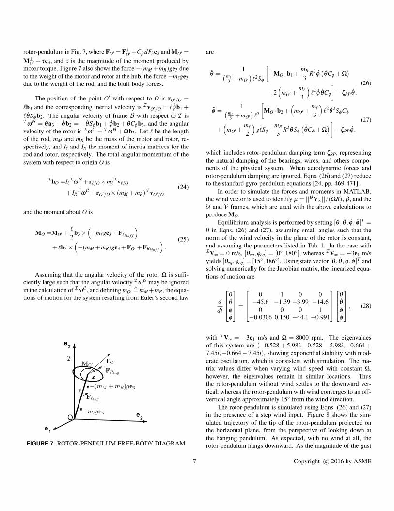
rotor-pendulum in Fig. 7, where FO′ =F⊥O′+Cβ dF3c3 and MO′ =

M⊥O′ + τc3, and τ is the magnitude of the moment produced bymotor torque. Figure 7 also shows the force−(mM +mR)ge3 dueto the weight of the motor and rotor at the hub, the force−m`ge3due to the weight of the rod, and the bluff body forces.

The position of the point O′ with respect to O is rO′/O =

`b3 and the corresponding inertial velocity is IvO′/O = `φb1 +

`θSφ b2. The angular velocity of frame B with respect to I isIωB = θa3 + φb2 = −θSφ b1 + φb2 + θCφ b3, and the angularvelocity of the rotor is IωC = IωB +Ωb3. Let ` be the lengthof the rod, mM and mR be the mass of the motor and rotor, re-spectively, and I` and IR the moment of inertia matrices for therod and rotor, respectively. The total angular momentum of thesystem with respect to origin O is

IhO =I`IωB+ r`/O×m`

Iv`/O

+ IRI

ωC + rO′/O× (mM +mR)

IvO′/O(24)

and the moment about O is

MO =MO′ +`

2b3×

(−m`ge3 +F`blu f f

)+ `b3×

(−(mM +mR)ge3 +FO′ +FRblu f f

).

(25)

Assuming that the angular velocity of the rotor Ω is suffi-ciently large such that the angular velocity IωB may be ignoredin the calculation of IωC , and defining mO′ ,mM+mR, the equa-tions of motion for the system resulting from Euler’s second law

-0.5

O

I

e3

ℓ

−mℓge3 e2

Rotor Gyropendulum

Fℓbluff

0

−(mM +mR)ge3

MO′

e1

FRbluff

FO′

-0.2

-0.2

0

0.2

0

0.4

e3

0.6

0.2

0.8

1

e1

e2

0.4 0.50.6 0.8 1

FIGURE 7: ROTOR-PENDULUM FREE-BODY DIAGRAM

are

θ =1(m`

3 +mO′)`2Sφ

[−MO ·b1 +

mR

3R2

φ(θCφ +Ω

)−2(

mO′ +m`

3

)`2

φ θCφ

]−ζRPθ ,

(26)

φ =1(m`

3 +mO′)`2

[MO ·b2 +

(mO′ +

m`

3

)`2

θ2SφCφ

+(

mO′ +m`

2

)g`Sφ−

mR

3R2

θSφ

(θCφ +Ω

)]−ζRPφ ,

(27)

which includes rotor-pendulum damping term ζRP, representingthe natural damping of the bearings, wires, and others compo-nents of the physical system. When aerodynamic forces androtor-pendulum damping are ignored, Eqns. (26) and (27) reduceto the standard gyro-pendulum equations [24, pp. 469-471].

In order to simulate the forces and moments in MATLAB,the wind vector is used to identify µ = ||BV∞||/(ΩR), β , and theU and V frames, which are used with the above calculations toproduce MO.

Equilibrium analysis is performed by setting [θ , θ , φ , φ ]T =0 in Eqns. (26) and (27), assuming small angles such that thenorm of the wind velocity in the plane of the rotor is constant,and assuming the parameters listed in Tab. 1. In the case withIV∞ = 0 m/s, [θeq,φeq] = [0,180], whereas IV∞ = −3e1 m/syields [θeq,φeq] = [15,186]. Using state vector [θ , θ ,φ , φ ]T andsolving numerically for the Jacobian matrix, the linearized equa-tions of motion are

ddt

θ

θ

φ

φ

=

0 1 0 0

−45.6 −1.39 −3.99 −14.60 0 0 1

−0.0306 0.150 −44.1 −0.991

θ

θ

φ

φ

, (28)

with IV∞ = −3e1 m/s and Ω = 8000 rpm. The eigenvaluesof this system are (−0.528 + 5.98i,−0.528− 5.98i,−0.664 +7.45i,−0.664−7.45i), showing exponential stability with mod-erate oscillation, which is consistent with simulation. The ma-trix values differ when varying wind speed with constant Ω,however, the eigenvalues remain in similar locations. Thusthe rotor-pendulum without wind settles to the downward ver-tical, whereas the rotor-pendulum with wind converges to an off-vertical angle approximately 15 from the wind direction.

The rotor-pendulum is simulated using Eqns. (26) and (27)in the presence of a step wind input. Figure 8 shows the sim-ulated trajectory of the tip of the rotor-pendulum projected onthe horizontal plane, from the perspective of looking down atthe hanging pendulum. As expected, with no wind at all, therotor-pendulum hangs downward. As the magnitude of the gust


Parameter Name Value Units

mR rotor mass 0.0027 kg

mM motor mass 0.018 kg

m` rod mass 0.043 kg

R rotor radius 0.0635 m

c chord length 0.015 m

Nb number of blades 2 [ ]

e effective hinge offset 0.1 [ ]

kβ hinge spring const. 3 Nm/rad

Iβ blade inertia 1.81×10−6 kgm2

ρ density of air 1.225 kg/m3

Clα airfoil lift slope 2π [ ]

γ Lock number 1.04 [ ]

λ0 avg. inflow ratio 0.075 [ ]

θ0 root angle of attack 16 deg

θtw blade twist -6.6 deg

ωβ0 spring nat. freq. 1290 rad/s

νβ blade scaled nat. freq. 1.9 [ ]

ζ blade damping coef. 0.026 [ ]

ζRP pendulum damp. coef. 1 [ ]

TABLE 1: MODEL PARAMETERS

increases, the vertical offset angle and magnitude of oscillationincrease, with the rotor-pendulum settling over time to the equi-librium value in the center of the oscillation. As the wind in-creases, the angle θ about the e3 axis reduces slightly due to thebluff body force, more closely aligning the pendulum to the winddirection.

EXPERIMENTIn order to validate the rotor-pendulum model, an experi-

mental stand (Fig. 9) was built and tested in a known wind fieldproduced by a set of blower-style Dyson fans (Fig. 10), with thesystem response identified using 18 OptiTrack motion-capturecameras. The rotor-pendulum test stand was initiated in thedownward position.

Tests were performed with a rotor speed of 8000 rpm andwind velocities of 0 m/s and −3e1 m/s. In order to verify the

-0.1 -0.05 0 0.05 0.1

e1 [m]

-0.08

-0.06

-0.04

-0.02

0

0.02

0.04

0.06

0.08

e2[m

] IV∞

4m/s3m/s2m/s1m/s0m/sφ = 180

FIGURE 8: SIMULATED ROTOR-PENDULUM

FIGURE 9: ROTOR-PENDULUM STAND

aerodynamic effects on the rotor, a disk with equal moment ofinertia was constructed using a 3D printer and also tested at bothwind speeds to investigate possible confounding variables. Asexpected, when testing without wind, both the rotor and disk ex-hibit stable equilibria at φ = 180 and arbitrary θ . Under a con-stant −3e1 m/s wind, the stable equilibrium point for the exper-imental stand with the rotor is [θeq,φeq] = [20,190], and withthe disk is [θeq,φeq] = [6,182]. This result indicates that even inthe case of the disk without lifting surfaces, the bluff body aero-dynamic drag of the system causes a change in the equilibrium


FIGURE 10: ROTOR-PENDULUM TEST FACILITY

point.A step input for wind from 0 to −3e1 m/s was generated by

quickly changing the angle of the blinds between the fans and thetest stand in Fig. 10 in order to maintain a smooth wind flow (asopposed to suddenly opening the blinds). Figure 11 shows theresult of this test, as well as a comparison to theoretical resultsunder the same conditions. Without the lifting surfaces of a rotor,bluff body drag moves the disk only slightly, and in the directionapproximately parallel to the wind direction as expected. Thepropeller also moves primarily in the direction of the wind, butat a much greater offset angle φ , and progresses in a spiral patternas it reaches its equilibrium point. This result shows the influenceof the lifting surfaces of the propeller, creating a higher momentthat also yields slight movement in the−e2 direction. Theoreticaland experimental results show strong agreement, indicating theimportance of linear inflow calculations in blade flapping analy-sis, which dramatically change the flap characteristics comparedto hover. Slight inaccuracy between the model and experiment ismost likely due to the aerodynamic complexity of the system.

CONCLUSIONThis paper presents a dynamic model of a rotor-pendulum

based on the aerodynamic response of a small, stiff propeller inwind. The model includes the blade-flapping response of the pro-peller and the resulting forces and moments. When simplified,the equations-of-motion reduce to those of a gyro-pendulum.State matrices and equilibrium points for the system under par-ticular conditions are numerically identified, showing a stablesystem with moderate oscillation in the presence of wind. Ex-perimental results show strong agreement with theoretical pre-dictions. Ongoing work includes analysis of the contributions of

-0.1 -0.05 0 0.05 0.1

e1 [m]

-0.08

-0.06

-0.04

-0.02

0

0.02

0.04

0.06

0.08

e2[m

] IV∞

Theoretical PropellerExperimental PropellerExperimental Diskφ = 180

FIGURE 11: ROTOR-PENDULUM EXPERIMENT

each of the forces and moments on the system in order to createa tractable model that can be implemented in real time for con-trol. Ongoing work resulting from this paper includes the devel-opment of a controllable quadrotor test stand that leverages theblade-flapping response, forces, and moments here to yield feed-back controllers capable of stabilizing the quadrotor in responseto a gust.

ACKNOWLEDGEMENTThis work was supported by the University of Maryland

Vertical Lift Rotorcraft Center of Excellence Army Grant No.W911W61120012. The authors would like to thank Dan Escobarand Elena Shrestha for providing parts and machining, as well asBharath Govindarajan and Andrew Lind for their blade-flappingand aerodynamics expertise.

REFERENCES[1] Rabbath, C., and Lechevin, N., 2010. Safety and Reliability

in Cooperating Unmanned Aerial Systems. World ScientificPublishing Co., Singapore, Chapter 1.

[2] Atkins, E. M., 2010. “Risk identification and managementfor safe UAS operation”. In Int. Symp. on Systems andControl in Aeronautics and Astronautics, Harbin, China,pp. 774–779.

[3] Zarovy, S., Costello, M., and Mehta, A., 2012. “Exper-imental method for studying gust effects on micro rotor-craft”. Proceedings of the Institution of Mechanical Engi-neers, 227(4), mar, pp. 703–713.

[4] Lu, H., Liu, C., Guo, L., and Chen, W.-H., 2015. “Flight


control design for small-scale helicopter using disturbance-observer-based backstepping”. Journal of Guidance, Con-trol, and Dynamics, 38(11), pp. 2235–2240.

[5] Garcıa Carrillo, L. R., Dzul Lopez, A. E., Lozano, R., andPegard, C., 2013. Quad rotorcraft control vision-based hov-ering and navigation. Springer, London, England, Chap-ter 2.

[6] Liu, H., Bai, Y., Lu, G., Shi, Z., and Zhong, Y., 2013. “Ro-bust tracking control of a quadrotor helicopter”. Journal ofIntelligent & Robotic Systems, 75(3-4), may, pp. 595–608.

[7] Mellinger, D., and Kumar, V., 2011. “Minimum snap trajec-tory generation and control for quadrotors”. In Proc. IEEEInt. Conf. Robotics and Automation, Shanghai, China,pp. 2520–2525.

[8] Lupashin, S., Schollig, A., Sherback, M., and D’Andrea,R., 2010. “A simple learning strategy for high-speedquadrocopter multi-flips”. In Proc. IEEE Int. Conf.Robotics and Automation, Anchorage, AK, pp. 1642–1648.

[9] Leishman, J. G., 2006. Principles of Helicopter Aerody-namics, 2nd ed. Cambridge University Press, New York,NY, Chapter 2,3,4.

[10] Mahony, R., Kumar, V., and Corke, P., 2012. “Modeling,estimation, and control of quadrotor”. IEEE Robotics andAutomation Magazine, sep, pp. 20–32.

[11] Bangura, M., and Mahony, R., 2012. “Nonlinear dy-namic modeling for high performance control of a quadro-tor”. In Proc. Australasian Conf. Robotics and Automation,Wellington, New Zealand, pp. 1–10.

[12] Hoffmann, G., Huang, H., Waslander, S., and Tomlin, C.,2007. “Quadrotor helicopter flight dynamics and control:theory and experiment”. In Proc. AIAA Guidance, Navi-gation, and Control Conf., Paper AIAA 2007-6461, HiltonHead, SC.

[13] Sydney, N., Smyth, B., and Paley, D., 2013. “Dynamic con-trol of autonomous quadrotor flight in an estimated windfield”. In Proc. IEEE Conf. Decision and Control, Firenze,Italy, pp. 3609–3616.

[14] Bristeau, P. J., Martin, P., Salaun, E., and Petit, N., 2009.“The role of propeller aerodynamics in the model of aquadrotor UAV”. In Proc. European Control Conference,Budapest, Hungary, pp. 683–688.

[15] Pounds, P., Mahony, R., and Corke, P., 2010. “Modellingand control of a large quadrotor robot”. Control Engineer-ing Practice, 18(7), pp. 691–699.

[16] Yeo, D., Sydney, N., and Paley, D. A., 2016. “Onboardflow sensing for rotary-wing UAV pitch control in wind”. InProc. AIAA Guidance Navigation and Control Conf., PaperAIAA 2016-1386, San Diego, CA.

[17] Prouty, R., 2005. Helicopter Performance, Stability, andControl. Krieger Publishing Company, Malabar, FL, Chap-ter 7.

[18] Niemiec, R., and Gandhi, F., 2016. “Effects of inflow

model on simulated aeromechanics of a quadrotor heli-copter”. In AHS International 72nd Annual Forum, WestPalm Beach, FL, pp. 1–13.

[19] Chen, R., 1989. A survey of nonuniform inflow models forrotorcraft flight dynamics and control applications. Tech.rep., NASA, Moffett Field, CA.

[20] Anderson, J. B., 2005. Carrier transmission. IEEE Press,Piscataway, NJ, Chapter 3.

[21] Hall, N., 2015. Shape Effects on Drag. On theWWW, June. URL http://www.grc.nasa.gov/WWW/k-12/airplane/shaped.html.

[22] Anderson, J. D., 1991. Fundamentals of Aerodynamics.McGraw-Hill, New York, NY, Chapter 4.

[23] Abbot, I., and Doenhoff, A., 1959. Theory of Wing Sec-tions. Dover Publications, New York, NY, Chapter 6.

[24] Kasdin, N. J., and Paley, D. A., 2011. Engineering Dynam-ics: A Comprehensive Introduction. Princeton UniversityPress, Princeton, NJ, Chapter 11.


dynamics of a rotor-pendulum with a small, …cdcl.umd.edu/papers/dscc16.pdf · ·...

Documents